Coalescence of black hole–neutron star binaries

Abstract

We review the current status of general relativistic studies for coalescences of black hole–neutron star binaries. First, high-precision computations of black hole–neutron star binaries in quasiequilibrium circular orbits are summarized, focusing on the quasiequilibrium sequences and the mass-shedding limit. Next, the current status of numerical-relativity simulations for the merger of black hole–neutron star binaries is described. We summarize our understanding for the merger process, tidal disruption and its criterion, properties of the merger remnant and ejected material, gravitational waveforms, and gravitational-wave spectra. We also discuss expected electromagnetic counterparts to black hole–neutron star coalescences.

1 Introduction

1.1 Why is the black hole–neutron star binary merger important?

After the first release of this review article in 2011 (Shibata and Taniguchi, 2011), the research environment for compact binary coalescences has changed completely. The turning point was the first gravitational-wave event GW150914 from a binary-black-hole merger detected by the LIGO and Virgo Collaboration (Abbott et al., 2016b). We obtained the strongest evidence for the existence of black holes and mergers of their binaries within the Hubble time. We learned that some stellar-mass black holes are significantly more massive than those found in our Galaxy by X-ray observations (Abbott et al., 2016a). Furthermore, we confirmed that general relativity is consistent with observations even for this dynamical and strongly gravitating phenomenon (Abbott et al., 2016c; Yunes et al., 2016, see also Abbott et al. 2019b, 2021c for the update). After further observations, the number of stellar-mass black holes detected by gravitational waves has already exceeded those by electromagnetic radiation (see Abbott et al. 2019a, 2021a for reported detections as of 2020). Gravitational-wave astronomy of binary black holes is rapidly becoming an established branch of astrophysics.

Subsequently, the first binary-neutron-star merger, GW170817, was detected with not only gravitational waves (Abbott et al., 2017d, 2019c) but also electromagnetic waves by multiband instruments all over the world (Abbott et al., 2017e, c). Tidal deformability of the neutron star was constrained from gravitational-wave data analysis, and extremely stiff equations of state are no longer favored (Abbott et al., 2017d; De et al., 2018; Abbott et al., 2018, 2019c; Narikawa et al., 2020). Binary-neutron-star mergers were strongly suggested to be central engines of short gamma-ray bursts by the detection of a weak GRB 170817A (Abbott et al., 2017c; Goldstein et al., 2017; Savchenko et al., 2017) and by longterm observations of its off-axis afterglow (Mooley et al., 2018a, b; Alexander et al., 2018; Lamb et al., 2019). The host galaxy NGC 4993 was identified by the kilonova/macronova AT 2017gfo (Coulter et al., 2017; Arcavi et al., 2017; Lipunov et al., 2017; Soares-Santos et al., 2017; Tanvir et al., 2017; Valenti et al., 2017), and Hubble’s constant was inferred in a novel manner by combining the cosmological redshift of NGC 4993 and the luminosity distance estimated from GW170817 (Abbott et al., 2017b). Furthermore, binary-neutron-star mergers were indicated to be a site of r-process nucleosynthesis (Tanaka et al., 2017; Kasen et al., 2017; Watson et al., 2019). This event heralded a new era of multimessenger astronomy with gravitational and electromagnetic radiation.

Finally, during the review process of this article, detections of black hole–neutron star binaries, GW200105 and GW200115, are reported (Abbott et al., 2021b). Together with another candidate of a black hole–neutron star binary merger GW190426_152155 (Abbott et al., 2021a), we may now safely consider that black hole–neutron star binaries are actually merging in our Universe. The merger rate is currently inferred to be $\approx 12$–$240\text{\,}\mathrm{G}\mathrm{p}\mathrm{c}^{-3}\,\mathrm{y}\mathrm{r}^{-1}$, which is largely consistent with previous theoretical estimation (Dominik et al., 2015; Kruckow et al., 2018; Neijssel et al., 2019; Zevin et al., 2020; Santoliquido et al., 2021, see also Narayan et al. 1991; Phinney 1991 for pioneering rate estimation). Unfortunately, despite the presence of neutron stars, no associated electromagnetic counterpart was detected. This is consistent with the current theoretical understanding reviewed throughout this article, because the most likely mass ratios of these binaries are as high as $4$–$5$ and the spin of the black holes are likely to be zero or retrograde. Tidal disruption do not occur for these parameters, and thus neither mass ejection nor electromagnetic emission is expected to occur. We also note that some other gravitational-wave events reported in LIGO-Virgo O3 are also consistent with black hole–neutron star binaries under generous assumptions on the mass of compact objects (Abbott et al., 2020a, c), partly because no electromagnetic counterpart was detected (Kyutoku et al., 2020; Han et al., 2020; Kawaguchi et al., 2020a).

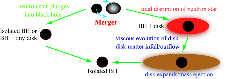
Figure 1: Summary for the merger and postmerger evolution of black hole–neutron star binaries. The fate is classified into two categories according to whether the neutron star is tidally disrupted (right) or not (left). Image adapted from Shibata and Hotokezaka (2019), copyright by Annual Reviews.

One of the remaining issues for ground-based gravitational-wave detectors is to discover coalescences of black hole–neutron star binaries accompanied by tidal disruption and hence electromagnetic emission. Indeed, among the mergers of black hole–neutron star binaries, those resulting in tidal disruption of the neutron star by the black hole are of physical and astrophysical interest and deserve detailed investigations. Specifically, the tidal disruption is required to occur outside the innermost stable circular orbit of the black hole for inducing astrophysically interesting outcomes. If the neutron star is not disrupted, as is likely the case of GW200105 and GW200115, it behaves like a point particle throughout the coalescence, and the merger process will be indistinguishable from that of (highly asymmetric) binary black holes (Foucart et al., 2013a) except for possible electromagnetic emission associated with crust shattering (Tsang et al., 2012), magnetospheric activities (Hansen and Lyutikov, 2001; McWilliams and Levin, 2011; Lai, 2012; Paschalidis et al., 2013; D’Orazio et al., 2016; Carrasco and Shibata, 2020; Wada et al., 2020; East et al., 2021; Carrasco et al., 2021, see also Ioka and Taniguchi 2000 for earlier work on binary neutron stars), or charged black holes (Levin et al., 2018; Zhang, 2019; Dai, 2019; Pan and Yang, 2019; Zhong et al., 2019). These two possibilities for the fate of merger are summarized schematically in Fig. 1.

Focusing on the cases in which tidal disruption occurs, many researchers have vigorously studied the following three aspects. Accordingly, most parts of this review will be devoted to their detailed discussions.

• Gravitational waves will enable us to study the finite-size properties and hence the equation of state of neutron stars. First, tidal deformability, $\Lambda$ (see also Sect. 1.3), of neutron stars will be extracted from the phase evolution in the inspiral phase (Flanagan and Hinderer, 2008) along with the masses and the spins of binary components (Finn and Chernoff, 1993; Jaranowski and Krolak, 1994; Cutler and Flanagan, 1994; Poisson and Will, 1995). Although the tidal deformability could be inferred even if tidal disruption does not occur, realistic measurements will be possible only when the finite-size effect is so sizable that the neutron star is disrupted (Lackey et al., 2012, 2014). Second, the orbital frequency at tidal disruption depends on the compactness of the neutron star, $\mathcal{C}$ (Vallisneri, 2000; Shibata et al., 2009). Because the mass can be extracted or constrained from inspiral signals along with the spin as stated above, gravitational waveforms from tidal disruption of a neutron star may bring us invaluable information about its radius, which is strongly but not perfectly correlated with the tidal deformability (Hotokezaka et al., 2016a; De et al., 2018). The measurement of these quantities with black hole–neutron star binaries could serve as an additional tool for exploring supranuclear-density matter (Lindblom, 1992; Harada, 2001). For this purpose, it is crucial to understand the dependence of gravitational waveforms, including characteristic observable features associated with tidal disruption, on possible equations of state by theoretical calculations.

• The remnant disk formed from the disrupted neutron star is a promising central engine of short-hard gamma-ray bursts (Paczynski, 1991; Narayan et al., 1992; Mochkovitch et al., 1993, see also Blinnikov et al. 1984 for an earlier idea and Paczynski 1986; Goodman 1986; Eichler et al. 1989 for binary-neutron-star scenarios). A typical beaming-corrected energy of the jet, $\sim${10}^{50}\text{\,}\mathrm{e}\mathrm{r}\mathrm{g}$$ (Fong et al., 2015), can be explained if, for example, $\sim 0.1\%$ of the rest-mass energy is converted from a $\sim 0.1\,M_{\odot}$ accretion disk. This could be realized via neutrino pair annihilation (Rees and Meszaros, 1992), which is effective when the disk is sufficiently hot and dense to cool via neutrino radiation, called the neutrino-dominated accretion flow (Popham et al., 1999; Narayan et al., 2001; Kohri and Mineshige, 2002; Di Matteo et al., 2002; Kohri et al., 2005; Chen and Beloborodov, 2007; Kawanaka and Mineshige, 2007). Another possible energy source is the rotational energy of a spinning black hole extracted by magnetic fields, i.e., the Blandford-Znajek mechanism (Blandford and Znajek, 1977; Mészáros and Rees, 1997). For this mechanism to work, magnetic-field strength in the disk needs to be amplified by turbulent motion resulting from magnetohydrodynamic instabilities such as the magnetorotational instability (Balbus and Hawley, 1991), and subsequently, strong magnetic fields threading the spinning black hole need to be developed to form a surrounding magnetosphere. One of the ultimate goals for numerical simulations of compact binary coalescences may be to clarify how, if possible, the ultrarelativistic jet is launched from the merger remnant. Theoretical investigations should also clarify whether longterm activity of short-hard gamma-ray bursts, e.g., the extended and plateau emission (Norris and Bonnell, 2006; Rowlinson et al., 2013; Gompertz et al., 2013; Kisaka et al., 2017), can really be explained by the merger remnant of black hole–neutron star binaries. Because of the diversity associated with stellar-mass black holes, black hole–neutron star binaries might naturally explain the variety observed in short-hard gamma-ray bursts (see Nakar 2007; Berger 2014 for reviews).

• A substantial amount of neutron-rich material will be ejected and synthesize r-process elements (Lattimer and Schramm, 1974, see also Lattimer 2019 for retrospection by an originator), i.e., about half of the elements heavier than iron in the universe, whose origin has not yet been fully understood (Burbidge et al., 1957; Cameron, 1957). Subsequently, radioactive decays of unstable nuclei will heat up the ejecta, resulting in quasithermal emission in UV-optical-IR bands on a time scale of $\order{10}$ days (Li and Paczyński, 1998). This transient, called the kilonova (Metzger et al., 2010b) or macronova (Kulkarni, 2005), serves as the most promising omnidirectional electromagnetic counterparts to gravitational waves (see Metzger 2019 for reviews). The ejecta are eventually mixed with the interstellar medium and contribute to the chemical evolution of galaxies, and this interaction may drive another electromagnetic counterpart such as synchrotron radiation from nonthermal electrons (Nakar and Piran, 2011) and possibly inverse Compton emission (Takami et al., 2014). To derive nucleosynthetic yields and characteristics of electromagnetic counterparts, we need to understand properties of the ejecta such as the mass, the velocity, and the electron fraction that characterizes the neutron richness. In particular, the electron fraction primarily determines the nucleosynthetic yield, which controls features of the kilonova/macronova via the opacity (Kasen et al., 2013; Tanaka and Hotokezaka, 2013; Tanaka et al., 2018, 2020; Banerjee et al., 2020) and the heating rate (Hotokezaka et al., 2016b; Barnes et al., 2016; Kasen and Barnes, 2019; Waxman et al., 2019; Hotokezaka and Nakar, 2020). If a significant fraction of the ejecta keeps extreme neutron richness of the neutron star, ultraheavy elements may be produced in abundance, and the associated fission and/or $\alpha$-decay will power the kilonova/macronova at late times (Wanajo et al., 2014; Zhu et al., 2018; Wu et al., 2019). They could also be the origin of exceptionally r-process enhanced metal-poor stars, so-called actinide-boost stars (see, e.g., Mashonkina et al., 2014). Last but not least, the geometrical shape of the ejecta could be important for understanding the diversity of electromagnetic counterparts to black hole–neutron star binaries (Kyutoku et al., 2013; Tanaka et al., 2014).

1.2 Life of black hole–neutron star binaries

We first overview the entire evolution of black hole–neutron star binaries from their birth. Binaries consisting of a black hole and/or a neutron star, hereafter collectively called compact object binaries, are generally born after evolution of isolated massive binaries (see, e.g., Postnov and Yungelson 2014 for reviews) or via dynamical processes in dense environments (see, e.g., Benacquista and Downing 2013 for reviews). Relative contributions of these two paths to black hole–neutron star binaries have not been understood yet, as well as for compact object binaries of other types. We do not go into details of the formation path in this article, commenting only that the evolution of isolated binaries is usually regarded as the dominant channel for black hole–neutron star binaries (see, e.g., discussions in Abbott et al., 2021b).

After the formation of black hole–neutron star binaries, their orbital separation decreases gradually due to longterm gravitational radiation reaction. If we would like to observe their coalescences, the binaries are required to merge within the Hubble time of $\approx$1.4\text{\times}{10}^{10}\text{\,}\mathrm{y}\mathrm{r}$$. This condition is also a prerequisite for them to drive short-hard gamma-ray bursts and to produce r-process elements. The lifetime of a black hole–neutron star binary in a circular orbit for a given orbital separation $r$ is given by

$$t_{\mathrm{GW}} =\frac{5c^{5}}{256G^{3}}\frac{r^{4}}{(M_{\mathrm{BH}}+M_{\mathrm{NS}})M_{\mathrm{BH}}M_{\mathrm{NS}}}$$

$$=$1.01\text{\times}{10}^{10}\text{\,}\mathrm{y}\mathrm{r}$\pqty{\frac{r}{$6\text{\times}{10}^{6}\text{\,}\mathrm{km}$}}^{4}\pqty{\frac{M_{\mathrm{BH}}}{7\,M_{\odot}}}^{-1}\pqty{\frac{M_{\mathrm{NS}}}{1.4\,M_{\odot}}}^{-1}\pqty{\frac{m_{0}}{8.4\,M_{\odot}}}^{-1}$$ (1)

in the adiabatic approximation, which is appropriate when the radiation reaction time scale is much longer than the orbital period. Here, $G$, $c$, $M_{\mathrm{BH}}$, $M_{\mathrm{NS}}$, and $m_{0}$ are the gravitational constant, the speed of light, the gravitational mass of the black hole, the gravitational mass of the neutron star, and the total mass of the binary $m_{0}:=M_{\mathrm{BH}}+M_{\mathrm{NS}}$, respectively (cf., Table 1). The orbital eccentricity only reduces the time to merger for a given value of the semimajor axis (Peters and Mathews, 1963; Peters, 1964). Thus, a black hole–neutron star binary merges within the Hubble time if its initial semimajor axis is smaller than $\sim${10}^{7}\text{\,}\mathrm{km}$$ with the precise value depending on the masses of the objects and the initial eccentricity. Because the spin and finite-size properties of the objects come into play only as higher-order corrections in terms of the orbital velocity or other appropriate parameters (see, e.g., Blanchet 2014 for reviews of the post-Newtonian formalism), Eq. (1) with eccentricity corrections is adequate for judging whether a binary merges within the Hubble time.

Two remarks should be made regarding the longterm evolution. First, the orbital eccentricity decreases rapidly, specifically $e\propto a^{-19/12}$ in an asymptotically circular regime with $a$ being the semimajor axis, due to gravitational radiation reaction (Peters, 1964). Accordingly, black hole–neutron star binaries right before merger (e.g., when gravitational waves are detected by ground-based detectors) may safely be approximated as circular. Second, the neutron star is unlikely to be tidally-locked, because the effects of viscosity are likely to be insufficient (Kochanek, 1992; Bildsten and Cutler, 1992). Thus, the spin of the neutron star can affect the merger dynamics significantly only if the rotational period is extremely short at the outset and the spin-down is not severe. Quantitatively, the dimensionless spin parameter of the neutron star is approximately written as

$$\chi_{\mathrm{NS}} =\frac{cI_{\mathrm{NS}}\Omega_{\mathrm{rot}}}{GM^{2}_{\mathrm{NS}}}=$4.9\text{\times}{10}^{-4}$\pqty{\frac{I_{\mathrm{NS}}/(M_{\mathrm{NS}}R_{\mathrm{NS}}^{2})}{1/3}}\pqty{\frac{M_{\mathrm{NS}}}{1.4\,M_{\odot}}}^{-1}\pqty{\frac{R_{\mathrm{NS}}}{$12\text{\,}\mathrm{km}$}}^{2}\pqty{\frac{P_{\mathrm{rot}}}{$1\text{\,}\mathrm{s}$}}^{-1},$$ (2)

where $I_{\mathrm{NS}}$, $R_{\mathrm{NS}}$, and $P_{\mathrm{rot}}$ are the moment of inertia, the radius, and the rotational period, respectively, of the neutron star. Observationally, the shortest rotational period of known pulsars in Galactic binary neutron stars that merge within the Hubble time is $\approx$17\text{\,}\mathrm{ms}$$, which is equivalent to only $\chi_{\mathrm{NS}}\approx 0.03$ (Stovall et al., 2018). Moreover, black hole–neutron star binaries are unlikely to harbor recycled pulsars, because the neutron star is expected to be formed after the black hole, having no chance for mass accretion. Hence, it is reasonable to approximate neutron stars as nonspinning in the merger of black hole–neutron star binaries. Exceptions to these remarks might arise from dynamical formation in dense environments such as galactic centers and globular clusters, e.g., exchange interactions involving recycled pulsars (see, e.g., Fragione et al., 2019; Ye et al., 2020), and/or black-hole formation from the secondary caused by mass transfer in isolated massive binaries (see, e.g., Kruckow et al., 2018).

The late inspiral and merger phases of black hole–neutron star binaries are promising targets of gravitational waves for ground-based detectors irrespective of the degree of tidal disruption. The frequency $f$ and the amplitude $h$ of gravitational waves from black hole–neutron star binaries with the orbital separation $r$ at the luminosity distance $D$ are estimated in the quadrupole approximation for two point particles as

$$f \approx\frac{\Omega}{\pi}=$523\text{\,}\mathrm{Hz}$\pqty{\frac{r}{6Gm_{0}/c^{2}}}^{-3/2}\pqty{\frac{m_{0}}{8.4\,M_{\odot}}}^{-1},$$ (3)

$$h \approx\frac{4G^{2}M_{\mathrm{BH}}M_{\mathrm{NS}}}{c^{4}rD}=$3.7\text{\times}{10}^{-22}$\pqty{\frac{\mu}{1.17\,M_{\odot}}}\pqty{\frac{r}{6Gm_{0}/c^{2}}}^{-1}\pqty{\frac{D}{$100\text{\,}\mathrm{M}\mathrm{p}\mathrm{c}$}}^{-1},$$ (4)

where $\mu:=M_{\mathrm{BH}}M_{\mathrm{NS}}/m_{0}$ is the reduced mass. Here, the most favorable direction and orientation are assumed for evaluating $h$. These values indicate that black hole–neutron star binaries near the end of their lives fall within the observable window of ground-based gravitational-wave detectors as far as the distance is sufficiently close.

However, the quadrupole approximation for point particles is not sufficiently accurate for describing the evolution of black hole–neutron star binaries in the late inspiral, merger, and postmerger phases. As the orbital separation gradually approaches the radius of the object, spins and finite-size effects such as tidal deformation begin to modify the gravitational interaction between the binary in a noticeable manner. The adiabatic approximation also breaks down for the very close orbit, because the radiation reaction time scale and the orbital period become comparable near an approximate innermost stable orbit as

$$\frac{t_{\mathrm{GW}}}{P_{\mathrm{orb}}}=2.0\pqty{\frac{r}{6Gm_{0}/c^{2}}}^{5/2}\pqty{\frac{M_{\mathrm{BH}}}{7\,M_{\odot}}}^{-1}\pqty{\frac{M_{\mathrm{NS}}}{1.4\,M_{\odot}}}^{-1}\pqty{\frac{m_{0}}{8.4\,M_{\odot}}}^{2}.$$ (5)

Thus, dynamics in the late inspiral and merger phases depends crucially on complicated hydrodynamics associated with neutron stars, whose properties are controlled by the equation of state, and on nonlinear gravity of general relativity. Furthermore, the evolution of the remnant disk in the postmerger phase is governed by neutrino emission triggered by shock-induced heating and turbulence associated with magnetohydrodynamic instabilities (Lee et al., 2004; Setiawan et al., 2004; Lee et al., 2005; Setiawan et al., 2006; Shibata et al., 2007). All these facts make fully general-relativistic numerical studies the unique tool to clarify the final evolution of black hole–neutron star coalescences in a quantitative manner.

1.3 Tidal problem around a black hole

As we stated in Sect. 1.1, this review will focus primarily on numerical studies of black hole–neutron star binaries for which finite-size effects play a significant role. To set the stage for understanding numerical results, in this Sect. 1.3, we will discuss requirement for the binary to cause significant tidal disruption, which starts with the mass shedding from the inner edge of the neutron star.

1.3.1 Mass-shedding condition

The orbital separation at which the mass shedding sets in is determined primarily by the mass ratio of the binary and the radius of the neutron star. The orbit at which the mass shedding sets in, the so-called mass-shedding limit, can be estimated semiquantitatively by Newtonian calculations as follows. Mass shedding from the neutron star occurs when the tidal force exerted by the black hole overcomes the self-gravity of the neutron star at the inner edge of the stellar surface. This condition is approximately given by

$$\frac{2GM_{\mathrm{BH}}(c_{\mathrm{R}}R_{\mathrm{NS}})}{r^{3}}\gtrsim\frac{GM_{\mathrm{NS}}}{(c_{\mathrm{R}}R_{\mathrm{NS}})^{2}},$$ (6)

where the factor $c_{\mathrm{R}}\geq 1$ represents the degree of tidal (and rotational if the neutron star is rapidly spinning) elongation of the stellar radius. The precise value of this factor depends on the neutron-star properties and the orbital separation. The mass-shedding limit may be defined as the orbit at which this inequality is approximately saturated,

$$r_{\mathrm{ms}}:=2^{1/3}c_{\mathrm{R}}\pqty{\frac{M_{\mathrm{BH}}}{M_{\mathrm{NS}}}}^{1/3}R_{\mathrm{NS}}.$$ (7)

We emphasize here that Eq. (6) is a necessary condition for the onset of mass shedding. Tidal disruption occurs only after substantial mass is stripped from the surface of the neutron star, while the orbital separation decreases continuously due to gravitational radiation reaction during this process. Thus, the tidal disruption should occur at a smaller orbital separation than Eq. (7). We also note that the neutron star will be disrupted immediately after the onset of mass shedding if its radius increases rapidly in response to the mass loss, although typical equations of state predict that the radius in equilibrium depends only weakly on the mass (see, e.g., Lattimer and Prakash 2016; Özel and Freire 2016; Oertel et al. 2017 for reviews).

Tidal disruption induces observable astrophysical consequences only if it occurs outside the innermost stable circular orbit of the black hole, inside which stable circular motion is prohibited by strong gravity of general relativity; If the tidal disruption fails to occur outside this orbit, the material is rapidly swallowed by the black hole and does not leave a remnant disk or unbound ejecta in an appreciable manner. This implies that observable tidal disruption requires, at least, the mass-shedding limit to be located outside the innermost stable circular orbit. The radius of the innermost stable circular orbit depends sensitively on the dimensionless spin parameter of the black hole, $\chi$. Specifically, it is given in terms of a dimensionless decreasing function $\hat{r}_{\mathrm{ISCO}}(\chi)$ of $\chi$ for an orbit on the equatorial plane of the black hole by (Bardeen et al., 1972)

$$r_{\mathrm{ISCO}}=\hat{r}_{\mathrm{ISCO}}(\chi)\frac{GM_{\mathrm{BH}}}{c^{2}}.$$ (8)

Here, we adopt the convention that the positive and negative values of $\chi$ indicate the prograde and retrograde orbits, i.e., the orbits with their angular momenta aligned and anti-aligned with the black-hole spin, respectively. Specifically, the value of $\hat{r}_{\mathrm{ISCO}}$ is $9$ for a retrograde orbit around an extremally-spinning black hole ($\chi=-1$), $6$ for an orbit around a nonspinning black hole ($\chi=0$), and $1$ for a prograde orbit around an extremally-spinning black hole ($\chi=1$). If the spin of the black hole is inclined with respect to the orbital angular momentum, the spin effect described here is not determined by the magnitude of the spin angular momentum but by that of the component parallel to the orbital angular momentum. Thus, even if the black-hole spin is high, its effect can be minor in the presence of spin misalignment.

To sum up, the final fate of a black hole–neutron star binary is determined primarily by the mass ratio of the binary, the compactness of the neutron star, and the dimensionless spin parameter of the black hole. The ratio of the radius of the mass-shedding limit and that of the innermost stable circular orbit is given by

$$\frac{r_{\mathrm{ms}}}{r_{\mathrm{ISCO}}}=\frac{2^{1/3}c_{\mathrm{R}}}{\hat{r}_{\mathrm{ISCO}}(\chi)}\pqty{\frac{M_{\mathrm{BH}}}{M_{\mathrm{NS}}}}^{-2/3}\pqty{\frac{GM_{\mathrm{NS}}}{c^{2}R_{\mathrm{NS}}}}^{-1}.$$ (9)

This semiquantitative estimate suggests that tidal disruption of a neutron star could occur if one or more of the following conditions are satisfied:

1. the mass ratio of the binary, $Q:=M_{\mathrm{BH}}/M_{\mathrm{NS}}$, is low,

2. the compactness of the neutron star, $\mathcal{C}:=GM_{\mathrm{NS}}/(c^{2}R_{\mathrm{NS}})$, is small,

3. the dimensionless spin parameter of the black hole, $\chi$, is high with the definition of signature stated above.

If we presume that the neutron-star mass is fixed, the conditions 1 and 2 may be restated as

1. the black-hole mass is small,

2. the neutron-star radius is large,

respectively.

Quantitative discussions have to take the general-relativistic nature of black hole–neutron star binaries into account. For this purpose, it is advantageous to rewrite Eq. (6) in terms of the orbital angular velocity as

$$\Omega^{2}\geq\frac{1}{2c_{\mathrm{R}}^{3}}\frac{GM_{\mathrm{NS}}}{R_{\mathrm{NS}}^{3}}\pqty{1+Q^{-1}},$$ (10)

because $\Omega$ can be defined in a gauge-invariant manner even for a comparable-mass binary in general relativity. It should be remarked that the orbital frequency at the onset of mass shedding is determined primarily by the average density of the neutron star, $\propto\sqrt{M_{\mathrm{NS}}/R_{\mathrm{NS}}^{3}}$. According to the results of fully general-relativistic numerical studies for quasiequilibrium states (Taniguchi et al., 2007, 2008, see Sect. 2 for the details), the mass-shedding condition is given by

$$\Omega^{2}\geq\Omega_{\mathrm{ms}}^{2}:=C_{\Omega}^{2}\frac{GM_{\mathrm{NS}}}{R_{\mathrm{NS}}^{3}}\pqty{1+Q^{-1}},$$ (11)

where $C_{\Omega}\lesssim 0.3$ for binaries of a nonspinning black hole and a neutron star with the irrotational velocity field. The smallness of $C_{\Omega}<1/\sqrt{2}$ indicates that the mass shedding is helped by significant tidal deformation, i.e., $c_{\mathrm{R}}>1$, and/or by relativistic gravity. This condition also indicates that the gravitational-wave frequency at the onset of mass shedding is given by

$$f_{\mathrm{ms}}=\frac{\Omega_{\mathrm{ms}}}{\pi}\gtrsim$1.0\text{\,}\mathrm{kHz}$\pqty{\frac{C_{\Omega}}{0.3}}\pqty{\frac{M_{\mathrm{NS}}}{1.4\,M_{\odot}}}^{1/2}\pqty{\frac{R_{\mathrm{NS}}}{$12\text{\,}\mathrm{km}$}}^{-3/2}\pqty{1+Q^{-1}}^{1/2}.$$ (12)

This value might be encouraging for ground-based gravitational-wave detectors, which have high sensitivity up to $\sim$1\text{\,}\mathrm{kHz}$$. However, we again caution that the mass shedding is merely a necessary condition for tidal disruption, and thus the frequency at tidal disruption should be higher than this value.

1.3.2 Tidal interaction in the orbital evolution

The discussion in Sect. 1.3.1 did not take the effect of tidal deformation of a neutron star on the orbital motion into account except for a fudge factor $c_{\mathrm{R}}$. Tidally-induced higher multipole moments of the neutron star modify the gravitational interaction between the binary components (see, e.g., Poisson and Will, 2014), so are the orbital evolution and the criterion for tidal disruption. This problem has thoroughly been investigated in Newtonian gravity with the ellipsoidal approximation, in which the isodensity contours are assumed to be self-similar ellipsoids (Lai et al., 1993b, a, 1994b, 1994a). They find that the tidal interaction acts as additional attractive force and accordingly the radius of the innermost stable circular orbit is increased (see also Rasio and Shapiro, 1992, 1994; Lai and Wiseman, 1996; Shibata, 1996). Because (i) the tidally-deformed neutron star develops a reduced quadrupole moment with the magnitude of components being $\propto r^{-3}$ associated with the tidal field of the black hole and (ii) the reduced quadrupole moment produces potential of the form $\propto r^{-3}$, the gravitational potential in the binary develops an $r^{-6}$ term in addition to the usual $r^{-1}$ term of the monopolar (i.e., mass) interaction. The reason that this interaction works as the attraction is that the neutron star is stretched along the line connecting the binary components and the enhancement of the pull at the inner edge dominates over the reduction at the outer edge. The steep dependence of the potential on the orbital separation indicates that the tidal interaction is especially important for determining properties of the close orbit.

These discussions about the tidal effects on the orbital motion have been revived in the context of gravitational-wave modeling and data analysis (Flanagan and Hinderer, 2008). Specifically, it has been pointed out that the finite-size effect of a star on the orbital evolution and hence gravitational waveforms are characterized quantitatively by the tidal deformability as far as the deformation is perturbative (Hinderer, 2008; Binnington and Poisson, 2009; Damour and Nagar, 2009). Because the additional attractive force increases the orbital angular velocity required to maintain a circular orbit for a given orbital separation, the gravitational-wave luminosity is also increased. In addition, the coupling of the quadrupole moments between the binary and the deformed star also enhances the luminosity. These effects accelerate the orbital decay particularly in the late inspiral phase to the extent that the difference of gravitational waveforms may be used to extract tidal deformability of neutron stars. This extraction has been realized in GW170817 (Abbott et al., 2017d, 2018; De et al., 2018; Abbott et al., 2019c; Narikawa et al., 2020) and GW190425 (Abbott et al., 2020a), whereas the statistical errors are large. It should also be cautioned that the effect of tidal deformability is not very large compared to various other effects, e.g., the spin and the eccentricity (Yagi and Yunes, 2014; Favata, 2014; Wade et al., 2014). In particular, the tidal effect comes into play effectively at the fifth post-Newtonian order ($r^{-6}/r^{-1}=r^{-5}$), but the point-particle terms at this order have not yet been derived in the post-Newtonian approximation. Thus, accurate extraction of tidal deformability requires sophistication not only in the description of tidal effects but also in the higher-order post-Newtonian corrections to point-particle, monopolar interactions. This fact has motivated gravitational-wave modeling in the effective-one-body formalism (Buonanno and Damour, 1999, 2000) and numerical relativity.

Tidal interaction and criteria for mass shedding in general relativity have long been explored for a circular orbit of a “test” Newtonian fluid star around a Kerr (or Schwarzschild) black hole as follows (Fishbone, 1973; Mashhoon, 1975; Lattimer and Schramm, 1976; Shibata, 1996; Wiggins and Lai, 2000; Ishii et al., 2005). The center of mass of the star is assumed to obey the geodesic equation in the background spacetime, and the stellar structure is computed with a model based on the Newtonian Euler’s equation of the form

$$\derivative{u_{i}}{\tau}=-\frac{1}{\rho}\partialderivative{P}{x^{i}}-\partialderivative{\phi}{x^{i}}-C_{ij}x^{j},$$ (13)

where $\tau$, $x^{i}$, $u_{i}$, $\rho$, $P$, $\phi$, and $C_{ij}$ denote the proper time of the stellar center, spatial coordinates orthogonal to the geodesic, the internal velocity, the rest-mass density, the pressure, the gravitational potential associated with the star itself, and the tidal tensor associated with the black hole, respectively. The self-gravity of the fluid star is computed in a Newtonian manner from Poisson’s equation sourced by $4\pi G\rho$. The tidal force of the black hole is incorporated up to the quadrupole order via the tidal tensor derived from the fully relativistic Riemann tensor (Marck, 1983, see also van de Meent 2020). Because the gravity of the fluid star is assumed not to affect the orbital motion and general relativity is not taken into account for describing its self-gravity, the analysis based on this model is valid quantitatively only for the cases in which the black hole is much heavier than the fluid star ($Q\gg 1$) and the fluid star is not compact ($\mathcal{C}\ll 1$). In addition, the tidal force of the black hole beyond the quadrupole order, $C_{ij}$, is neglected (Marck, 1983), and this model is valid only if the stellar radius is much smaller than the curvature scale of the background spacetime (again, $Q\gg 1$ is assumed). Regarding this point, higher-order tidal interactions have also been incorporated (Ishii et al., 2005) via the tidal potential computed in the Fermi normal coordinates (Manasse and Misner, 1963).

A series of analysis described above confirms the qualitative dependence of the mass-shedding and tidal-disruption conditions inferred from Eq. (9) on binary parameters in a semiquantitative manner. Specifically, the mass shedding from an incompressible star is found to occur for the mass and the spin of the black hole satisfying

$$M_{\mathrm{BH}}\lesssim C_{M}(\chi)\,M_{\odot}\pqty{\frac{M_{\mathrm{NS}}}{1.4\,M_{\odot}}}^{-1/2}\pqty{\frac{R_{\mathrm{NS}}}{$10\text{\,}\mathrm{km}$}}^{3/2},$$ (14)

where $C_{M}(0)\approx 4.6$, $C_{M}(0.5)\approx 7.8$, $C_{M}(0.75)\approx 12$, $C_{M}(0.9)\approx 19$, and $C_{M}(1)\approx 68$ (Shibata, 1996). This condition tells us that tidal disruption of a neutron star by a nonspinning black hole is possible only if the black-hole mass is small compared to astrophysically typical values (see, e.g., Özel et al., 2010; Kreidberg et al., 2012; Abbott et al., 2019a, 2021a). At the same time, the increase in the threshold mass by a factor of $\approx 15$ for extremal black holes is impressive particularly in light of many massive black holes discovered by gravitational-wave observations.

The threshold mass of the black hole for mass shedding and thus tidal disruption also depends on the neutron-star equation of state even if the mass and the radius are identical (Wiggins and Lai, 2000; Ishii et al., 2005). If we focus on polytropes, stiffer equations of state characterized by a larger adiabatic index are more susceptible to tidal deformation due to the flatter, less centrally condensed density profile. Conversely, neutron stars with a soft equation of state are less subject to tidal disruption than those with a stiff one. These features are also reflected in the tidal Love number and tidal deformability (Hinderer, 2008). Note that the incompressible model corresponds to the stiffest possible equation of state. According to the computations performed adopting compressible stellar models (Wiggins and Lai, 2000; Ishii et al., 2005), the threshold mass of the black hole may be reduced by 10%–20% for a soft equation of state characterized by a small adiabatic index.

In reality, the self-gravity of the neutron star needs to be treated in a general-relativistic manner. General-relativistic effects associated with the neutron star have been investigated by a series of work in a phenomenological manner based on the ellipsoidal approximation (Ferrari et al., 2009, 2010; Pannarale et al., 2011; Ferrari et al., 2012; Maselli et al., 2012). However, quantitative understanding of the mass shedding and tidal disruption ultimately requires numerical computations of quasiequilibrium states and dynamical simulations of the merger process in full general relativity.

1.4 Brief history of studies on black hole–neutron star binaries

Here, we briefly review studies on black hole–neutron star binaries from the historical perspectives in an approximate chronological order. We also introduce pioneering studies that are not fully relativistic, e.g., Newtonian computations of equilibrium states and partially-relativistic simulations of the coalescences. In the main part of this article, Sect. 2 and Sect. 3, we will review fully general-relativistic results, i.e., quasiequilibrium states satisfying the Einstein constraint equations and dynamical evolution derived by solving the full Einstein equation, from the physical perspectives.

1.4.1 Nonrelativistic equilibrium computation

Equilibrium configurations of a neutron star governed by Newtonian self-gravity in general-relativistic gravitational fields of a background black hole was first studied in Fishbone (1973) for incompressible fluids in the corotational motion (i.e., the fluid is at rest in the corotating frame of the binary). The criterion for mass shedding was investigated and qualitative results were obtained. This type of studies has been generalized to accommodate irrotational velocity fields (i.e., the vorticity is absent; Shibata, 1996), compressible, polytropic equations of state (Wiggins and Lai, 2000), and higher-order tidal potential of the black hole (Ishii et al., 2005). Another direction of extension was to remove the assumption of the extreme mass ratio of the binary. This extension was done in Taniguchi and Nakamura (1996) by adopting modified pseudo-Newtonian potential for the black hole based on the so-called Paczyński–Wiita potential (Paczyńsky and Wiita, 1980) to determine the location of the innermost stable circular orbit.

However, all these studies have limitation even if we accept the Newtonian self-gravity of neutron stars. The ellipsoidal approximation is strictly valid only if the fluid is incompressible and the tidal field beyond the quadrupole order can be neglected (Chandrasekhar, 1969). Thus, the internal structure of compressible neutron stars in a close orbit can be investigated only qualitatively.

The hydrostationary equilibrium of black hole–neutron star binaries was derived in Uryū and Eriguchi (1998) assuming that the black hole was a point source of Newtonian gravity and that the neutron star with irrotational velocity fields obeyed a polytropic equation of state (irrotational Roche–Riemann problem). The center-of-mass motion of the neutron star was computed fully accounting for its self-gravity, and the tidal field of the Newtonian point source was incorporated to the full order in the ratio of the stellar radius to the orbital separation. Their subsequent work, Uryū and Eriguchi (1999), considered both the corotational and irrotational velocity fields, and differences from the ellipsoidal approximation have been analyzed.

1.4.2 Relativistic quasiequilibrium computation

One of the essential features of general relativity is the existence of gravitational radiation, whose reaction prohibits exactly stationary equilibria of binaries. Still, an approximately stationary solution to the Einstein equation may be obtained by solving the constraint equations, quasiequilibrium conditions derived by some of the evolution equations, and hydrostationary equations. Such solutions are called quasiequilibrium states, and Eq. (5) suggests that they are reasonable approximations to inspiraling binaries except near merger (see also Blackburn and Detweiler, 1992; Detweiler, 1994). The quasiequilibrium states are important not only by their own but also as initial data of realistic numerical-relativity simulations.

Quasiequilibrium states and sequences of black hole–neutron star binaries in full general relativity were first studied in Miller (2001) with preliminary formulation. Approximate quasiequilibrium states in the extreme mass ratio limit were obtained for the corotational velocity field in Baumgarte et al. (2004) and later for the irrotational velocity field in Taniguchi et al. (2005). Because gravitational fields around the black hole are not required to be solved in the extreme mass ratio limit, these computations were performed only around (relativistic) neutron stars.

General-relativistic quasiequilibrium states for comparable-mass binaries were obtained in 2006 by various groups both in the excision (Grandclément, 2006; Taniguchi et al., 2006) and the puncture frameworks (Shibata and Uryū, 2006, 2007). A general issue in the numerical computation of black-hole spacetimes is how to handle the associated physical or coordinate singularity. The excision framework handles the black hole by removing the interior of a suitably-defined horizon (see, e.g., Dreyer et al., 2003; Ashtekar and Krishnan, 2004; Gourgoulhon and Jaramillo, 2006) from the computational domains and by imposing appropriate boundary conditions (Cook, 2002; Cook and Pfeiffer, 2004). The puncture framework separates the singular and regular components in an analytic manner so that only the latter terms are solved numerically (Bowen and York, 1980; Brandt and Brügmann, 1997). The details are presented in Appendix A.

Taniguchi et al. (2007) derived accurate quasiequilibrium sequences in the excision framework by adopting the conformally-flat background and investigated properties of close black hole–irrotational neutron star binaries such as the mass-shedding limit (see also Grandclément, 2007). Taniguchi et al. (2008) further improved the sequences by enforcing nonspinning conditions for the black hole in a sophisticated manner via the boundary condition at the horizon. Quasiequilibrium states with spinning black holes were computed with the same code as initial data for numerical simulations (Etienne et al., 2009).

Quasiequilibrium states in the puncture framework were also derived for irrotational velocity fields in Shibata and Taniguchi (2008) by extending the formulation for corotating neutron stars (Shibata and Uryū, 2006, 2007). Kyutoku et al. (2009) obtained quasiequilibrium sequences of nonspinning black holes with varying the method for determining the center of mass of the binary, which is not uniquely defined in the puncture framework. Quasiequilibrium states in the puncture framework were extended to black holes with aligned and inclined spins (Kyutoku et al., 2011a; Kawaguchi et al., 2015), and the same formulation has also been adopted to perform merger simulations in the conformal-flatness approximation (Just et al., 2015). Recently, the eccentricity reduction method has been implemented in this framework (Kyutoku et al., 2021, see below for preceding work in the excision framework).

Except for early work in the puncture framework (Shibata and Uryū, 2006, 2007), all the computations described above were performed with the spectral-method library, LORENE, which enables us to achieve very high precision (see Grandclément and Novak 2009 for reviews). Note that Grandclément (Grandclément, 2006) and Taniguchi (Taniguchi et al., 2006) are two of the main developers of LORENE.

Foucart et al. (2008) also computed quasiequilibrium sequences in the excision framework with an independent code, SPELLS (Pfeiffer et al., 2003). This code implemented a modified Kerr-Schild background metric for computing highly-spinning black holes (Lovelace et al., 2008) and the eccentricity reduction method for performing realistic inspiral simulations (Pfeiffer et al., 2007). Initial data with inclined black-hole spins were also derived (Foucart et al., 2011). The computations of quasiequilibrium states have now been extended to high-compactness (Henriksson et al., 2016) and/or spinning neutron stars (Tacik et al., 2016). Papenfort et al. (2021) have also derived quasiequilibrium sequences by using another spectral-method library, KADATH (Grandclément, 2010).

1.4.3 Non/partially-relativistic merger simulations

The merger process of black hole–neutron star binaries was first studied in Newtonian gravity primarily with the aim of assessing the potentiality for the central engine of gamma-ray bursts. In the early work, the black hole was modeled by a point source of Newtonian gravity with (artificial) absorbing boundary conditions. A series of simulations with a smoothed-particle-hydrodynamics code explored influences of the rotational states of the fluids and stiffness of the (polytropic) equations of state for neutron-star matter (Kluźniak and Lee, 1998; Lee and Kluźniak, 1999b, a; Lee, 2000, 2001). They studied the process of tidal disruption, subsequent formation of a black hole–disk system and mass ejection, properties of the remnant disk and unbound material, and gravitational waveforms emitted during merger.

Around the same time, Janka et al. (1999) performed simulations incorporating detailed microphysics with a mesh-based hydrodynamics code. Specifically, their code had implemented a temperature- and composition-dependent equation of state (Lattimer and Swesty, 1991) and neutrino emission modeled in terms of the leakage scheme (Ruffert et al., 1996). By performing simulations for various configurations of binaries, a hot and massive remnant disk with $\gtrsim$10\text{\,}\mathrm{MeV}$$ and $0.2$–$0.7\,M_{\odot}$ was suggested to be formed, and the neutrino luminosity was found to reach ${10}^{53}$–${10}^{54}\text{\,}\mathrm{e}\mathrm{r}\mathrm{g}\,\mathrm{s}^{-1}$ during 10–$20\text{\,}\mathrm{ms}$ after formation of a massive disk. Pair annihilation of neutrinos was also investigated by post-process calculations (Ruffert et al., 1997) and was found to be capable of explaining the total energy of gamma-ray bursts. Although these Newtonian results were still highly qualitative and both the disk mass and temperature can be overestimated for given binary parameters (see below), it was first suggested by dynamical simulations that black hole–neutron star binary coalescences could be promising candidates for the central engine of short-hard gamma-ray bursts if the massive accretion disk was indeed formed. Rosswog et al. (2004) also performed simulations in similar setups with a smoothed-particle-hydrodynamics code adopting a different equation of state (Shen et al., 1998).

The gravity in the vicinity of a black hole modeled by a Newtonian point source is qualitatively different from that in reality. In particular, the innermost stable circular orbit is absent in the Newtonian point-particle model. Because of this difference, early Newtonian work concluded that the neutron star might be disrupted without an immediate plunge even in an orbit closer to the black hole than $\lesssim 6GM_{\mathrm{BH}}/c^{2}$. Consequently, they indicated that a massive remnant disk with $\gtrsim 0.1\,M_{\odot}$ might be formed around the black hole irrespective of the mass ratio and the rotational states of fluids. It should also be mentioned that the orbital evolution within Newtonian gravity frequently exhibited episodic mass transfer (see Clark and Eardley 1977; Cameron and Iben 1986; Benz et al. 1990 for relevant discussions). That is, the neutron star is only partially disrupted via the stable mass transfer during the close encounter with the black hole, becomes a “mini-neutron star” (Rosswog, 2005) with increasing the binary separation, and continues the orbital motion. This has never been found in fully relativistic simulations (although not completely rejected throughout the possible parameter space) and may be regarded as another qualitative difference associated with the realism of gravitation (see also Appendix C.1).

To overcome these drawbacks, Rosswog (2005) performed smoothed-particle-hydrodynamics simulations by modeling the black-hole gravity in terms of a pseudo-Newtonian potential (Paczyńsky and Wiita, 1980). A potential for modeling the gravity of a spinning black hole (Artemova et al., 1996) was also adopted in later mesh-based simulations (Ruffert and Janka, 2010), and the episodic mass transfer was still observed for some parameters of binaries. These work found that the massive disk with $\gtrsim 0.1\,M_{\odot}$ was formed only for binaries with low-mass and/or spinning black holes. Because this feature agrees qualitatively with the fully relativistic results, simulations with a pseudo-Newtonian potential might be helpful to understand the nature of black hole–neutron star binary mergers qualitatively or even semiquantitatively.

While numerical-relativity simulations have been feasible since 2006 (see Sect. 1.4.4), approximately general-relativistic simulations have also been performed without simplifying the black holes by point sources of gravity. This is particularly the case of smoothed-particle-hydrodynamics codes, which are especially useful to track the motion of the material ejected from the system but have not been available in numerical relativity (see Rosswog and Diener 2021 for recent development). One of the popular approaches to incorporate general relativity is the conformal-flatness approximation (Faber et al., 2006a, b; Just et al., 2015). In these work, the gravity of neutron stars was also treated in a general-relativistic manner. Another work adopted the Kerr background for modeling the black hole, while the neutron star is modeled as a Newtonian self-gravitating object, and studied dependence of the merger process on the inclination angle of the black-hole spin with respect to the orbital angular momentum (Rantsiou et al., 2008). Results of these simulations agree qualitatively with those from pseudo-Newtonian and numerical-relativity simulations.

1.4.4 Fully-relativistic merger simulations

General-relativistic effects play a crucial role in the dynamics of close black hole–neutron star binaries. First of all, the inspiral is driven by gravitational radiation reaction. Dynamics right before merger is affected crucially by further general-relativistic effects, which include strong attractive force between two bodies, associated presence of the innermost stable circular orbit, spin-orbit coupling, and relativistic self-gravity of neutron stars. Accordingly, the orbital evolution, the merger process, the criterion for tidal disruption, and the evolution of disrupted material are all affected substantially by the general-relativistic effects. Although non-general-relativistic work has provided qualitative insights, numerical simulations in full general relativity are obviously required for accurately and quantitatively understanding the nature of black hole–neutron star binary coalescences. This is particularly the case in development of an accurate gravitational-wave template for the data analysis.

Soon after the breakthrough success in simulating binary-black-hole mergers (Pretorius, 2005; Campanelli et al., 2006; Baker et al., 2006), Shibata and Uryū (2006, 2007); Shibata and Taniguchi (2008) started exploration of black hole–neutron star binary coalescences in full general relativity extending their early work on binary neutron stars (Shibata, 1999; Shibata and Uryū, 2000, 2002; Shibata et al., 2003, 2005; Shibata and Taniguchi, 2006). While these work adopted initial data computed in the puncture framework for moving-puncture simulations, Etienne et al. (2008) independently performed moving-puncture simulations with excision-based initial data by extending their early work on binary neutron stars (Duez et al., 2003, see also Löffler et al. 2006 for early work on a head-on collision in a similar setup). Duez et al. (2008) also performed simulations for black hole–neutron star binaries based on the excision method by introducing hydrodynamics equation solvers to a spectral-method code, SpEC, for binary black holes (Boyle et al., 2007, 2008; Scheel et al., 2009). All these studies were performed for nonspinning black holes and neutron stars modeled by a polytropic equation of state with $\Gamma=2$.

To derive accurate gravitational waveforms, longterm simulations need to be performed. Effort in this direction was made with the aid of an adaptive-mesh-refinement code (see Appendix B.3), SACRA (Yamamoto et al., 2008), by the authors (Shibata et al., 2009, 2012). Around the same time, Etienne et al. (2009) independently studied the effect of black-hole spins by another adaptive-mesh-refinement code. Systematic longterm studies were started employing nuclear-theory based equations of state approximated by piecewise-polytropic equations of state (Read et al., 2009a) for both nonspinning (Kyutoku et al., 2010, 2011b) and spinning black holes (Kyutoku et al., 2011a). A tabulated, temperature- and composition-dependent equation of state (Shen et al., 1998) was also incorporated in simulations with SpEC around the same time (Duez et al., 2010), while neutrino reactions were not considered in this early work. SpEC was also used to simulate systems with inclined black-hole spins (Foucart et al., 2011) or an increased mass ratio of $Q=7$ (Foucart et al., 2012). These simulations clarified quantitatively the criterion for tidal disruption, properties of the remnant disk and black hole, and emitted gravitational waves in the merger phase.

Mass ejection from black hole–neutron star binaries and associated fallback of material began to be explored in numerical relativity at the beginning of 2010’s (Chawla et al., 2010; Kyutoku et al., 2011a). Actually, these studies predate the corresponding investigations for binary neutron stars in numerical relativity (Hotokezaka et al., 2013b). Although the authors of this article suggested that $\geq 0.01\,M_{\odot}$ may be ejected dynamically from black hole–neutron star binaries in this early work (Kyutoku et al., 2011a), they were unable to show the ejection of material with confidence, partly because the artificial atmosphere was not tenuous enough and the computational domains were not large enough. By contrast, the mass ejection from hyperbolic encounters was discussed clearly (Stephens et al., 2011; East et al., 2012, 2015).

Serious investigations of the dynamical mass ejection were initiated in 2013 (Foucart et al., 2013b; Lovelace et al., 2013; Kyutoku et al., 2013), right after the first version of this review article was released, stimulated by the importance of electromagnetic counterparts to gravitational waves (Abbott et al., 2020b, the preprint version of which appeared on arXiv in 2013). Kyutoku et al. (2015) systematically studied kinematic properties such as the mass and the velocity as well as the morphology of dynamical ejecta with reducing the density of artificial atmospheres and enlarging the computational domains. Kawaguchi et al. (2015) also investigated the impact of the inclination angle of the black-hole spin for both the remnant disk and the dynamical ejecta (see also Foucart et al., 2013b). The study of mass ejection has now become routine in numerical-relativity simulations of black hole–neutron star binary coalescences. Accordingly, a lot of discussions about mass ejection are newly added in this update.

The current frontier of numerical relativity for neutron-star mergers is the incorporation of magnetohydrodynamics and neutrino-radiation hydrodynamics as accurately as possible. These physical processes play essentially no role during the inspiral phase (Chawla et al., 2010; Etienne et al., 2012a, c; Deaton et al., 2013), and thus gravitational radiation, disk formation, and dynamical mass ejection are safely studied by pure hydrodynamics simulations except for the chemical composition of the dynamical ejecta. However, both neutrinos and magnetic fields are key agents for driving postmerger evolution including disk outflows and ultrarelativistic jets. In addition, the electron fraction of the ejected material, either dynamical or postmerger, can be quantified only by simulations implementing composition-dependent equations of state with appropriate schemes for neutrino transport.

Although numerical-relativity codes for magnetohydrodynamics were already available in the late 2000’s and a preliminary simulation was performed by Chawla et al. (2010), magnetohydrodynamics simulations are destined to struggle with the need to resolve short-wavelength modes of instability (see, e.g., Balbus and Hawley 1998 for reviews). Various simulations have been performed aiming at clarifying the launch of an ultrarelativistic jet, generally finding magnetic-field amplification difficult to resolve (Etienne et al., 2012a, c). The situation was much improved by high-resolution simulations performed in Kiuchi et al. (2015b, see also for a follow-up). At around the same time, magnetohydrodynamics simulations with a presumed strong dipolar field have been performed to clarify the potentiality of black hole–neutron star binaries as a central engine of short-hard gamma-ray bursts (Paschalidis et al., 2015; Ruiz et al., 2018, 2020). Simulations beyond ideal magnetohydrodynamics have recently been performed aiming at clarifying magnetospheric activities right before merger (East et al., 2021).

As the electron fraction of the ejected material is crucial to determine the nucleosynthetic yield and the feature of associated kilonovae/macronovae, numerical-relativity simulations with neutrino transport have been performed extensively following those for binary-neutron-star mergers (Sekiguchi et al., 2011b, a). Neutrino-radiation-hydrodynamics simulations of black hole–neutron star binaries were first performed in Deaton et al. (2013); Foucart et al. (2014, 2017); Brege et al. (2018) with neutrino emission based on a leakage scheme (see Ruffert et al., 1996; Rosswog and Liebendörfer, 2003, for the description in Newtonian cases) and with composition-dependent equations of state. These simulations are also capable of predicting neutrino emission from the postmerger system. Kyutoku et al. (2018) incorporated neutrino absorption by the material based on the two moment formalism (Thorne, 1981; Shibata et al., 2011) again following work on binary neutron stars (Wanajo et al., 2014; Sekiguchi et al., 2015).

The longterm postmerger evolution of the remnant accretion disk also requires numerical investigations. These simulations need to be performed with sophisticated microphysics, because the evolution of the disk is governed by weak interaction processes such as the neutrino emission and absorption and magnetohydrodynamical processes. The liberated gravitational binding energy may eventually be tapped to launch a postmerger wind as well as an ultrarelativistic jet. Simulations focusing on the postmerger evolution with detailed neutrino transport are initially performed without incorporating sources of viscosity for a short term (Foucart et al., 2015). This work has been extended in the Cowling approximation to incorporate magnetic fields that provide effective viscosity and induce magnetohydrodynamical effects (Hossein Nouri et al., 2018). Fujibayashi et al. (2020a, b) performed fully-general-relativistic viscous-hydrodynamics simulations for postmerger systems with detailed neutrino transport. Finally, Most et al. (2021b) reported results of postmerger simulations for nearly-equal-mass black hole–neutron star binaries with neutrino transport and magnetohydrodynamics in full general relativity. Still, it is not feasible to perform fully-general-relativistic simulations incorporating both detailed neutrino transport and well-resolved magnetohydrodynamics. Because the postmerger mass ejection is now widely recognized as an essential source of nucleosynthesis and electromagnetic emission for binary-neutron-star mergers (Shibata et al., 2017a), sophisticated simulations for this problem will remain the central topic in the future study of black hole–neutron star binary coalescences.

After the detection of gravitational waves from binary neutron stars GW170817 (Abbott et al., 2017d) and GW190425 (Abbott et al., 2020a), it became apparent that robust characterization of source properties requires us to distinguish binary neutron stars from black hole–neutron star binaries (see Sect. 4.2.2). This situation motivated studies on mergers of very-low-mass black hole–neutron star binaries to clarify disk formation, mass ejection, and gravitational-wave emission in a more precise manner than what was done before (Foucart et al., 2019b; Hayashi et al., 2021; Most et al., 2021a). Here, “very low mass” means that it is consistent with being a neutron star and that observationally distinguishing binary types is not straightforward. Interestingly, these studies are revealing overlooked features of very-low-mass ratio systems. Finally, longterm simulations with $\gtrsim 10$–$15$ inspiral orbits have recently been performed aiming at deriving accurate gravitational waveforms (Foucart et al., 2019a, 2021).

1.5 Outline and notation

This review article is organized as follows. In Sect. 2, we review the current status of the study on quasiequilibrium states of black hole–neutron star binaries in general relativity. First, we summarize physical parameters characterizing a binary in Sect. 2.1. Next, the parameter space surveyed is summarized in Sect. 2.2. Results and implications are reviewed in Sect. 2.3 and Sect. 2.4, respectively. In Sect. 3, we review the current status of the study on coalescences of black hole–neutron star binaries in numerical relativity. Methods for numerical simulations are briefly described in Sect. 3.1, and the parameter space investigated is summarized in Sect. 3.2. The remainder of Sect. 3 is devoted to reviewing numerical results, and readers interested only in them should jump into Sect. 3.3, in which we start from reviewing the overall process of the binary coalescence and tidal disruption in the late inspiral and merger phases. Properties of the remnant disk, remnant black hole, fallback material, and dynamical ejecta are summarized in Sect. 3.4. Postmerger evolution of the remnant disk is reviewed in Sect. 3.5. Gravitational waveforms and spectra are reviewed in Sect. 3.6. Finally in Sect. 4, we discuss implications of numerical results to electromagnetic emission and characterization of observed astrophysical sources. Formalisms to derive quasiequilibrium states and to simulate dynamical evolution are reviewed in Appendix A and Appendix B, respectively. Appendix C presents analytic estimates related to discussions made in this article.

Table 1: List of symbols

symbol	content
	geometric quantity
$g_{\mu\nu}$	spacetime metric
$g$	determinant of $g_{\mu\nu}$
$\nabla_{\mu}$	covariant derivative associated with $g_{\mu\nu}$
$\Sigma_{t}$	three-dimensional hypersurface of a constant time $t$
$n^{\mu}$	future-directed timelike unit vector normal to $\Sigma_{t}$
$\alpha$	lapse function
$\beta^{i}$	shift vector
$\gamma_{\mu\nu}$	induced metric $\gamma_{\mu\nu}:=g_{\mu\nu}+n_{\mu}n_{\nu}$ on $\Sigma_{t}$
$D_{i}$	covariant derivative associated with $\gamma_{ij}$
$\gamma$	determinant of $\gamma_{ij}$; $\sqrt{-g}=\alpha\sqrt{\gamma}$
$K_{ij}$	extrinsic curvature on $\Sigma_{t}$
$K$	trace of the extrinsic curvature $K:=\gamma^{ij}K_{ij}$
	hydrodynamical quantity
$T^{\mu\nu}$	energy–momentum tensor
$u^{\mu}$	four velocity of the fluid
$v^{i}$	three velocity of the fluid $u^{i}/u^{t}$
$w$	Lorentz factor of the fluid $\alpha u^{t}$
$\rho$	baryon rest-mass density
$\varepsilon$	specific internal energy
$P$	pressure
$h$	specific enthalpy $h:=c^{2}+\varepsilon+P/\rho$
$T$	temperature
$Y_{\mathrm{e}}$	electron fraction
$\kappa$	polytropic constant
$\Gamma$	adiabatic index
$\alpha_{\nu}$	alpha parameter for the viscosity à la Shakura and Sunyaev (1973)
	parameter of the black hole
$M_{\mathrm{BH}}$	gravitational mass of the black hole in isolation
$S_{\mathrm{BH}}$	spin angular momentum of the black hole
$\chi$	dimensionless spin parameter of the black hole $\chi:=cS_{\mathrm{BH}}/(GM_{\mathrm{BH}}^{2})$
$\iota$	inclination angle of the black-hole spin with respect to the orbital plane
	parameter of the neutron star
$M_{\mathrm{NS}}$	gravitational mass of the neutron star in isolation
$M_{\mathrm{B}}$	baryon rest mass of the neutron star
$R_{\mathrm{NS}}$	circumferential radius of a spherical neutron star in isolation
$\mathcal{C}$	compactness of the neutron star $\mathcal{C}:=GM_{\mathrm{NS}}/(c^{2}R_{\mathrm{NS}}$)
	binary parameter
$m_{0}$	gravitational mass of the binary at infinite separation $m_{0}:=M_{\mathrm{BH}}+M_{\mathrm{NS}}$
$Q$	mass ratio of the binary $Q:=M_{\mathrm{BH}}/M_{\mathrm{NS}}$
$\Omega$	orbital angular velocity of the binary
$f$	gravitational-wave frequency

The notation adopted in this article is summarized in Table 1. Among the parameters shown in this table, $M_{\mathrm{BH}}$, $\chi$, $\iota$, $M_{\mathrm{NS}}$, and $R_{\mathrm{NS}}$ are frequently used to characterize binary systems in this article. The negative value of $\chi$ is allowed for describing anti-aligned spins, meaning that the dimensionless spin parameter and the inclination angle are given by $\absolutevalue{\chi}$ and $\iota=$$$, respectively. Hereafter, the dimensionless spin parameter is referred to also by the spin parameter for simplicity. Greek and Latin indices denote the spacetime and space components, respectively. We adopt geometrical units in which $G=c=1$ in Sect. 2, Sect. 3.6, Appendix A, and Appendix B.

This article focuses on fully general-relativistic studies of black hole–neutron star binaries, and other types of compact object binaries are not covered in a comprehensive manner. Numerical-relativity simulations of compact object binaries in general are reviewed in, e.g., Lehner and Pretorius (2014); Duez and Zlochower (2019). Simulations of compact object binaries involving neutron stars and their implications for electromagnetic counterparts are reviewed in, e.g., Paschalidis (2017); Baiotti and Rezzolla (2017); Shibata and Hotokezaka (2019). Black hole–neutron star binaries are also reviewed briefly in Foucart (2020).

2 Quasiequilibrium state and sequence

Quasiequilibrium states of compact object binaries in close orbits are important from two perspectives. First, they enable us to understand deeply the tidal interaction of comparable-mass binaries in general relativity. Second, they serve as realistic initial conditions for dynamical simulations in numerical relativity.

For the purpose of the former, a sequence of quasiequilibrium states parametrized by the orbital separation or angular velocity, i.e., quasiequilibrium sequences, should be investigated as an approximate model for the evolution path of the binary. In this section, we review representative numerical results of quasiequilibrium sequences derived to date. The formulation to construct black hole–neutron star binaries in quasiequilibrium is summarized in Appendix A. Because the differential equations to be solved are typically of elliptic type (see also the end of this section), most numerical computations adopt spectral methods for achieving high precision (see Grandclément and Novak 2009 for reviews). In this section, geometrical units in which $G=c=1$ is adopted.

2.1 Physical parameters of the binary

In this Sect. 2.1, we present physical quantities required for quantitative analysis of quasiequilibrium sequences. Each sequence is specified by physical quantities conserved at least approximately along the sequences, and these quantities also serve as labels of binary models in dynamical simulations. We also need physical quantities that characterize each quasiequilibrium state to study its property.

To begin with, we introduce a helical Killing vector used in modeling quasiequilibrium states of black hole–neutron star binaries (see also Appendix A). Because the time scale of gravitational radiation reaction is much longer than the orbital period except for binaries in a very close orbit as we discussed in Sect. 1.2, the binary system appears approximately stationary in the comoving frame. Such a system is considered to be in quasiequilibrium and is usually modeled by assuming the existence of a helical Killing vector with the form of

$$\xi^{\mu}=(\partial_{t})^{\mu}+\Omega(\partial_{\varphi})^{\mu},$$ (15)

where $\Omega$ denotes the orbital angular velocity of the system. The helical Killing vector is timelike and spacelike in the near zone of $\varpi\lesssim c/\Omega$ and the far zone of $\varpi\gtrsim c/\Omega$, respectively, where $\varpi$ denotes the distance from the rotational axis and we inserted $c$ for clarity. Thus, if we focus only on quasiequilibrium configurations in the near zone, we may assume the existence of a timelike Killing vector, which allows us to define several physical quantities in a meaningful manner.

Here, it is necessary to keep the following two (not independent) caveats in mind if we consider helically symmetric spacetimes. First, spacetimes of binaries cannot be completely helically symmetric in full general relativity. That is, it is not realistic to assume that a helical Killing vector exists in the entire spacetime. The reason is that the helical symmetry holds throughout the spacetime only if standing gravitational waves are present everywhere. However, the total energy of the system diverges for such a case. Thus, the helical Killing vector can be supposed to exist only in a limited region of the spacetime, e.g., in the local wave zone. A simpler strategy for studying quasiequilibrium states of a binary is to neglect the presence of gravitational waves. Although this is an overly simplified assumption, this strategy has been employed in the study of quasiequilibrium states of compact object binaries. The results introduced in this section are derived by assuming that gravitational waves are absent. Moreover, the induced metric is assumed to be conformally flat (see Appendix A for the details.)

Second, gravitational radiation reaction violates the helical symmetry in full general relativity. To compute realistic quasiequilibrium states of compact object binaries, we need to take radiation reaction into account. Procedures for this are described in Appendix A.5.2.

2.1.1 Parameters of the black hole

It is reasonable to assume that the irreducible mass (i.e., the area of the event horizon) and the magnitude of the spin angular momentum of the black hole are conserved along a quasiequilibrium sequence, because the absorption of gravitational waves by the black hole is only a tiny effect (Alvi, 2001; Chatziioannou et al., 2013, see also Poisson and Sasaki 1995; Poisson 2004 for relevant work in black-hole perturbation theory). The irreducible mass of the black hole is defined by (Christodoulou, 1970)

$$M_{\mathrm{irr}}:=\sqrt{\frac{A_{\mathrm{EH}}}{16\pi}},$$ (16)

where $A_{\mathrm{EH}}$ is the proper area of the event horizon. Because the event horizon cannot be identified in quasiequilibrium configurations, its area, $A_{\mathrm{EH}}$, is usually approximated by that of the apparent horizon, $A_{\mathrm{AH}}$. It is reasonable to consider that $A_{\mathrm{AH}}$ agrees at least approximately with $A_{\mathrm{EH}}$ in the current context, because a timelike Killing vector is assumed to exist in the vicinity of the black hole (Hawking and Ellis, 1973, Chap. 9). The magnitude of the spin angular momentum is determined in terms of an approximate Killing vector $\xi_{\mathcal{S}}^{i}$ for axisymmetry on the horizon as (Dreyer et al., 2003; Caudill et al., 2006)

$$S_{\mathrm{BH}}:=\frac{1}{8\pi}\oint_{\mathcal{S}}\pqty{K_{ij}-K\gamma_{ij}}\xi_{\mathcal{S}}^{j}\differential{S}^{i}.$$ (17)

An approximate Killing vector, $\xi_{\mathcal{S}}^{i}$, may be determined on the horizon by requiring some properties satisfied by genuine Killing vectors to hold (see Appendix A.1.1).

The angle of the black-hole spin angular momentum is usually evaluated in terms of coordinate-dependent quantities specific to individual formulations, because no geometric definition is known. It should be cautioned that the direction of the black-hole spin seen from a distant observer changes for the case in which the precession motion occurs (Apostolatos et al., 1994). Still, the angle between the black-hole spin and the orbital angular momentum of the binary is approximately conserved during the evolution, and hence, can be employed to characterize the system.

The gravitational mass (sometimes called the Christodoulou mass; Christodoulou, 1970) of the black hole in isolation is given by

$$M_{\mathrm{BH}}^{2}=M_{\mathrm{irr}}^{2}+\frac{S_{\mathrm{BH}}^{2}}{4M_{\mathrm{irr}}^{2}}.$$ (18)

By introducing a dimensionless spin parameter of the black hole,

$$\chi:=\frac{S_{\mathrm{BH}}}{M_{\mathrm{BH}}^{2}},$$ (19)

the gravitational mass is also written by

$$M_{\mathrm{BH}}=M_{\mathrm{irr}}\bqty{\frac{2}{1+(1-\chi^{2})^{1/2}}}^{1/2}.$$ (20)

Because $M_{\mathrm{BH}}$ is directly measured in actual observations, this quantity rather than $M_{\mathrm{irr}}$ is usually adopted to label quasiequilibrium sequences and the models of binary systems in dynamical simulations for spinning black holes, along with the spin parameter, $\chi$.

2.1.2 Parameters of the neutron star

The baryon rest mass of the neutron star given by

$$M_{\mathrm{B}}=\int\rho u^{t}\sqrt{-g}\differential[3]{x}=\int\rho\alpha u^{t}\sqrt{\gamma}\differential[3]{x}$$ (21)

is conserved along quasiequilibrium sequences assuming that the continuity equation holds and that mass ejection from the neutron star does not occur prior to merger. The spin angular momentum of the neutron star may be evaluated on the stellar surface by Eq. (17) (Tacik et al., 2016), although it is not conserved on a long time scale due to the spin-down. The orientation of the spin is also affected by the precession motion.

In contrast to black holes, an equation of state needs to be provided to specify finite-size properties of neutron stars such as the radius and the tidal deformability, although the realistic equation of state at supranuclear density is still uncertain (see, e.g., Lattimer and Prakash 2016; Oertel et al. 2017; Baym et al. 2018 for reviews). Because of rapid cooling by neutrino emission in the initial stage and subsequent photon emission (see, e.g., Potekhin et al. 2015 for reviews), temperature of not-so-young neutron stars relevant to coalescing compact object binaries is likely to be much lower than the Fermi energy of constituent particles. Thus, it is reasonable to adopt a fixed zero-temperature equation of state throughout the quasiequilibrium sequence. The zero-temperature equation of state allows us to express all the thermodynamic quantities as functions of a single variable, e.g., the rest-mass density.

As a qualitative model, the polytrope of the form

$$P(\rho)=\kappa\rho^{\Gamma},$$ (22)

where $\kappa$ and $\Gamma$ are the polytropic constant and the adiabatic index, respectively, has often been adopted in the study of quasiequilibrium sequences. The neutron-star matter is frequently approximated by a polytrope with $\Gamma\approx 2$–3. More sophisticated models include piecewise polytropes (Read et al., 2009a) and generalization thereof (O’Boyle et al., 2020), spectral representations (Lindblom, 2010), and various nuclear-theory-based tabulated equations of state. We will come back to this topic later in Sect. 3.1.2.

Once a hypothetical equation of state is given, the gravitational mass of a neutron star in isolation, $M_{\mathrm{NS}}$, is determined for a given value of the baryon rest mass, $M_{\mathrm{B}}$, via the Tolman-Oppenheimer-Volkoff equation (Tolman, 1939; Oppenheimer and Volkoff, 1939) [if the neutron star is spinning, the magnitude of the spin also comes into play (Hartle, 1967; Friedman and Stergioulas, 2013)]. The gravitational mass rather than the baryon rest mass is usually adopted to label the models of dynamical simulations, primarily because the gravitational mass is directly measured in actual observations. The equation of state also determines the radius and the compactness for a given mass of the neutron star. By imposing perturbative tidal fields on a background spherical configuration, the tidal deformability as a function of the neutron-star mass is computed from the ratio of the tidally-induced multipole moment and the exerted tidal field (Hinderer, 2008; Binnington and Poisson, 2009; Damour and Nagar, 2009).

2.1.3 Parameters of the binary system

The Arnowitt–Deser–Misner (ADM) mass of the system (Arnowitt et al., 2008) is evaluated in isotropic Cartesian coordinates (see, e.g., York 1979, Chap. 8; Gourgoulhon 2012, Chap. 8 for further details) as

$$M_{\mathrm{ADM}}=-\frac{1}{2\pi}\oint_{r\to\infty}\partial_{i}\psi\differential{S}^{i},$$ (23)

where $\psi$ is the conformal factor, which is given by $\psi=\gamma^{1/12}$ in Cartesian coordinates for a conformally-flat case (see Appendix A). This quantity should decrease as the orbital separation decreases along a quasiequilibrium sequence because of the strengthening of gravitational binding. The binding energy of a binary system is often defined by

$$E_{\mathrm{b}}:=M_{\mathrm{ADM}}-m_{0},$$ (24)

where the total mass $m_{0}:=M_{\mathrm{BH}}+M_{\mathrm{NS}}$ corresponds to the ADM mass of the binary system at infinite orbital separation.

The Komar mass is originally defined as a charge associated with a timelike Killing vector (Komar, 1959) and is evaluated in the $3+1$ formulation by (see, e.g., Shibata, 2016, Sect. 5)

$$M_{\mathrm{K}}=\frac{1}{4\pi}\oint_{r\to\infty}\pqty{\partial_{i}\alpha-K_{ij}\beta^{j}}\differential{S}^{i}.$$ (25)

Since quasiequilibrium states of black hole–neutron star binaries are computed assuming the existence of a helical Killing vector which is timelike in the near zone, the Komar mass may be considered as a physical quantity, at least approximately. If the second term in the integral falls off sufficiently rapidly, as is typical for the case in which the linear momentum of the system vanishes, the Komar mass may be evaluated only from the first term, i.e., the derivative of the lapse function. Because the ADM and Komar masses should agree if a timelike Killing vector exists (Friedman et al., 2002; Shibata et al., 2004, see also Beig 1978; Ashtekar and Magnon-Ashtekar 1979), their fractional difference,

$$\delta M:=\absolutevalue{\frac{M_{\mathrm{ADM}}-M_{\mathrm{K}}}{M_{\mathrm{ADM}}}},$$ (26)

measures the global error in the numerical computation. This quantity is sometimes called the virial error.

An ADM-like angular momentum of the system may be defined by (York, 1979)

$$J_{i}:=\frac{1}{16\pi}\underline{\epsilon}_{ijk}\oint_{r\to\infty}\pqty{X^{j}K^{kl}-X^{k}K^{jl}}\differential{S}_{l},$$ (27)

where $X^{i}$ and $\underline{\epsilon}_{ijk}$ denote, respectively, Cartesian coordinates relative to the center of mass of the binary and the Levi-Civita tensor for the flat space. It should be cautioned that this quantity is well-defined only in restricted coordinate systems (see, e.g., York, 1979; Gourgoulhon, 2012, Chap. 8). This subtlety is irrelevant to the results reviewed in this article. For binary systems with the reflection symmetry about the orbital plane, only the component normal to the plane is nonvanishing and will be denoted by $J$.

2.2 Current parameter space surveyed

Table 2: Summary of the study on quasiequilibrium sequences. The first column points to the references. The other columns are explained in the body text. We do not list references which present individual quasiequilibrium states, including initial data for dynamical simulations.

Reference	Metric	Hole	Spin	Flow	EOS	Compactness	Mass Ratio
Taniguchi et al. (2006)	KS	Ex	$0$	Ir	Poly	$0.088$	$5$
Taniguchi et al. (2007)	CFMS	Ex	$0$	Ir	Poly	$0.088,0.145$	$1$–$10$
Taniguchi et al. (2008)	CFMS	Ex	$0$	Ir	Poly	$0.109$–$0.132$	$1$–$9$
Grandclément (2006, 2007)	CFMS	Ex	0	Ir	Poly	$0.075$–$0.150$	$5$
Shibata and Uryū (2006)	CFMS	Pu	$0$	Co	Poly	$0.139$	$2.47$
Shibata and Uryū (2007)	CFMS	Pu	$0$	Co	Poly	$0.139,0.148$	$2.47,3.08$
Kyutoku et al. (2009)	CFMS	Pu	$0$	Ir	Poly	$0.132,0.145,0.160$	$1,3,5$
Foucart et al. (2008)	CFMS	Ex	$0$	Ir	Poly	$0.144$	$1$
	MKS	Ex	$-0.5,0$	Ir	Poly	$0.144$	$1$
Henriksson et al. (2016)	MKS	Ex	$0$	Ir	Tab	$0.23,0.25$	$6$
Papenfort et al. (2021)	CFMS	Ex	$0$	Ir	Poly	$0.138$	$1$

Although a decade has passed since the release of the first version of this article, the parameter space surveyed for the study of quasiequilibrium sequences remains narrow. The main progress achieved during this period may be the computations of sequences involving high-compactness neutron stars with a tabulated equation of state (Henriksson et al., 2016). We classify the current study shown in Table 2 according to the following seven items (see Appendix A for the details).

1. Metric: Choice of the spatial background metric $\hat{\gamma}_{ij}$ and the extrinsic curvature $K$. The abbreviations “CFMS,” “KS,” and “MKS” mean, respectively, the conformally-flat and maximal-slicing condition ($K=0$; see Appendix A.1), Kerr-Schild, and modified Kerr-Schild.

2. Hole: Method to handle the singularity associated with the black hole. The abbreviations “Ex” and “Pu” indicate the excision and the puncture approaches, respectively.

3. Spin: Dimensionless spin parameter of the black hole $\chi$. Note that the spin is zero or anti-aligned with the orbital angular momentum in these work.

4. Flow: State of the fluid flow in the neutron star. The abbreviations “Ir” and “Co” indicate irrotational and corotational flows, respectively. Arbitrary spins of neutron stars are not considered in these computations.

5. EOS: Equation of state for neutron-star matter. Here, “Poly” means the polytrope (specifically, that with $\Gamma=2$) and “Tab” means a tabulated equation of state. Specifically, the SLy equation of state (Douchin and Haensel, 2001) is adopted for computing quasiequilibrium sequences in Henriksson et al. (2016).

6. Compactness: Compactness of the neutron star $\mathcal{C}$.

7. Mass Ratio: Mass ratio $Q$.

Quasiequilibrium sequences with high and/or misaligned spins of either component have not been derived. Meanwhile, computations of individual quasiequilibrium states have been extended to a wide range of the parameter space including spin vectors for both black holes and neutron stars (Tacik et al., 2016). Additionally, many quasiequilibrium configurations, including those with a radial approaching velocity to reduce the orbital eccentricity (Foucart et al., 2008; Kyutoku et al., 2021), have been computed as initial conditions of dynamical simulations, whose results will be discussed in Sect. 3.

2.3 Numerical results

Hereafter in this section, we focus on the results reported in Taniguchi et al. (2008), because a systematic survey for a wide range of the parameter space was performed only there. Accordingly, all the results are derived in the excision approach, the conformal-flatness and maximal-slicing condition, nonspinning black holes, the irrotational flow, and the $\Gamma=2$ polytrope. Still, this work reasonably captures the properties of quasiequilibrium sequences. As the polytropic equation of state has only a single dimensional parameter, $\kappa$, we may normalize various quantities such as the length, mass, and time by the polytropic length scale,

$$R_{\mathrm{poly}}:=\kappa^{1/(2\Gamma-2)}\bqty{=\kappa^{1/(2\Gamma-2)}G^{-1/2}c^{(\Gamma-2)/(\Gamma-1)}}.$$ (28)

We will put an overbar above a symbol for indicating quantities in the polytropic unit, e.g., $\bar{M}_{\mathrm{B}}:=M_{\mathrm{B}}/R_{\mathrm{Poly}}[=GM_{\mathrm{B}}/(c^{2}R_{\mathrm{poly}})]$.

Figure 2: Contour of the conformal factor, $\psi$, on the orbital plane for the innermost configuration with the mass ratio $Q=3$ and the baryon rest mass of the neutron star $\bar{M}_{\mathrm{B}}=0.15$ ($\mathcal{C}=0.145$). The cross symbol indicates the position of the rotational axis. Image reproduced with permission from Taniguchi et al. (2008), copyright by APS.

Figure 2 displays contours of the conformal factor, $\psi$, for a black hole–neutron star binary with the mass ratio $Q=3$ and the baryon rest mass of the neutron star $\bar{M}_{\mathrm{B}}=0.15$ ($\mathcal{C}=0.145$). This contour plot shows the configuration at the smallest orbital separation for which the code used in Taniguchi et al. (2008) successfully achieved a converged solution. The thick solid circle for $X<0$ (left) denotes the excised surface, i.e., the apparent horizon, while that for $X>0$ (right) denotes the surface of the neutron star. A saddle point exists between the black hole and the neutron star, and for this close orbit, it is located in the vicinity of the inner edge of the neutron star. This fact suggests that the orbit of the binary is close to the mass-shedding limit. The value of $\psi$ on the excised surface is not constant, because a Neumann boundary condition is imposed (see Appendix A.1.1).

2.3.1 Binding energy and total angular momentum

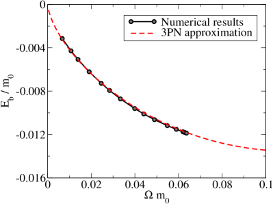
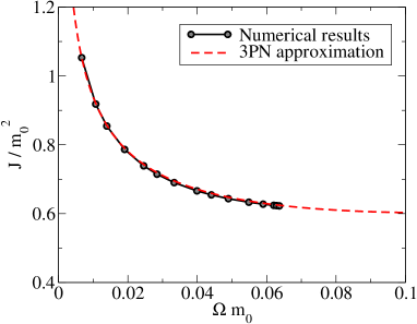
Figure 3: Binding energy $E_{\mathrm{b}}/m_{0}[=E_{\mathrm{b}}/(m_{0}c^{2})]$ (left) and total angular momentum $J/m_{0}^{2}[=cJ/(Gm_{0}^{2})]$ (right) as functions of $\Omega m_{0}(=G\Omega m_{0}/c^{3})$ for binaries with $Q=3$ and $\bar{M}_{\mathrm{B}}=0.15$ ($\mathcal{C}=0.145$). The solid curve with the filled circles shows numerical results, and the dashed curve denotes the results derived in the third-order post-Newtonian approximation for point particles (Blanchet, 2002). Image reproduced with permission from Taniguchi et al. (2008), copyright by APS.

Figure 3 shows the binding energy, $E_{\mathrm{b}}/m_{0}[=E_{\mathrm{b}}/(m_{0}c^{2})]$, and the total angular momentum, $J/m_{0}^{2}[=cJ/(Gm_{0}^{2})]$, as functions of the orbital angular velocity, $\Omega m_{0}(=G\Omega m_{0}/c^{3})$, for a binary with $Q=3$ and $\bar{M}_{\mathrm{B}}=0.15$ ($\mathcal{C}=0.145$). All the quantities of the binary are expressed as dimensionless quantities normalized by the total mass, $m_{0}$. This figure shows that the numerical results agree quantitatively with the third-order post-Newtonian approximation (Blanchet, 2002). The results also agree with the up-to-date, fourth-order post-Newtonian approximations (Blanchet, 2014), which differ only by $<1\%$ and $<3\%$ for the binding energy and the total angular momentum, respectively, from the third-order ones in the range of $\Omega m_{0}$ considered here. For this parameter set, the numerical sequence terminates at the mass-shedding limit, i.e., at an orbit for which a cusp is formed at the inner edge of the neutron star and the material begins to flow out, before the innermost stable circular orbit is encountered, i.e., before the minimum of the binding energy appears.

If the binary separation at the mass-shedding limit is substantially larger than the radius of the innermost stable circular orbit, the neutron star is expected not only to start shedding mass but also to be tidally disrupted before being swallowed by the black hole. Equation (9) presented in Sect. 1.3.1 suggests that the ratio of the binary separation at the mass-shedding limit to the radius of the innermost stable circular orbit decreases with increasing the mass ratio, $Q$, and/or the compactness of the neutron star, $\mathcal{C}$. Thus, it is naturally expected that quasiequilibrium sequences encounter minima in the binding energy and the total angular momentum as in the two-point-particle problem in general relativity, if the mass ratio is sufficiently high and/or the compactness is sufficiently large.

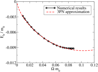
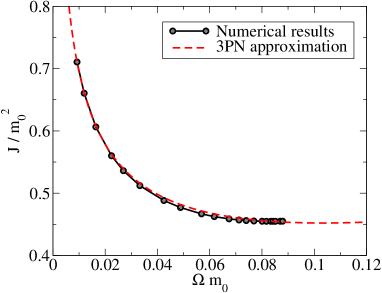
Figure 4: Same as Fig. 3 but for the sequence with $Q=5$. Image reproduced with permission from Taniguchi et al. (2008), copyright by APS.

Figure 4 shows the binding energy, $E_{\mathrm{b}}/m_{0}$, and the total angular momentum, $J/m_{0}^{2}$, as functions of $\Omega m_{0}$ for a binary with $Q=5$ and $\bar{M}_{\mathrm{B}}=0.15$ ($\mathcal{C}=0.145$). While the compactness of the neutron star is the same as that shown in Fig. 3, the mass ratio is higher. In this sequence, an innermost stable circular orbit is encountered before the onset of mass shedding, i.e., we see minima in the binding energy and the angular momentum just before the end of the sequence.

Figure 5: Binding energy as a function of the total angular momentum for binaries with $Q=5$ and different compactnesses of neutron stars. The solid curve denotes the results derived in the third-order post-Newtonian approximation for point particles (Blanchet, 2002). Image reproduced with permission from Taniguchi et al. (2008), copyright by APS.

Figure 4 shows that the turning points in the binding energy and the total angular momentum appear simultaneously within the numerical accuracy as described by theory of binary thermodynamics (Friedman et al., 2002). A simultaneous turning point appears as a cusp in the curve representing the relation between the binding energy and the total angular momentum. This fact is clearly seen in Fig. 5, which shows the relations for sequences with $Q=5$ but with different compactnesses of neutron stars. As suggested by Eq. (9), turning points are not found for small compactnesses such as $\mathcal{C}=0.120$, since the sequences terminate at mass shedding before encountering an innermost stable circular orbit. By contrast, for large compactnesses, these curves indeed form a cusp. Note that sequences derived in post-Newtonian approximations for point particles cannot identify mass shedding and therefore always exhibit turning points. The difference of $E_{\mathrm{b}}/m_{0}$ as a function of $J/m_{0}^{2}$ between the third- and fourth-order post-Newtonian approximations is less than 0.1% before the binary reaches an innermost stable circular orbit for the binary parameters chosen here. Although it may appear from Fig. 5 that the numerical results deviate from the post-Newtonian approximation as the compactness increases, i.e., approaching a point-particle limit, quasiequilibrium sequences of binary black holes also deviate from the analytic computation based on the post-Newtonian approximation in a similar manner to the high-compactness sequence of black hole–neutron star binaries (Cook and Pfeiffer, 2004; Caudill et al., 2006).

2.4 Endpoint of the sequence

One of the most important questions in the study of black hole–neutron star binaries is whether the coalescence leads to mass shedding of the neutron star before reaching the innermost stable circular orbit or to the plunge of the neutron star into the black hole before the onset of mass shedding. The answer to this question is essential for the topics raised in Sect. 1.1: Orbital dynamics and gravitational waves in the late inspiral and merger phases are affected strongly by this issue, and hence, its precise understanding is necessary for developing theoretical templates. For driving a short-hard gamma-ray burst, formation of an accretion disk surrounding the black hole is the most promising model. The r-process nucleosynthesis and electromagnetic emission occur if the material of the neutron star is ejected from the system. Both the disk formation and the mass ejection can result only if the neutron star is disrupted prior to reaching the innermost stable circular orbit.

Quantitative exploration of this issue ultimately requires dynamical simulations, and their results will be reviewed in Sect. 3. However, in-depth studies of quasiequilibrium sequences also provide a guide to the binary parameters that separate mass shedding and the dynamical plunge. In the following, we summarize quantitative insights obtained from the study of quasiequilibrium sequences. Specifically, we will review semiquantitative expressions that may be used to predict whether a black hole–neutron star binary of arbitrary values of $Q$ and $\mathcal{C}$ encounters an innermost stable circular orbit before the onset of mass shedding or not. Since the detailed study was performed only for nonspinning black holes, we do not consider the effect of black-hole spins in the following. However, as discussed in Sect. 1.3, we have to keep in mind that the spin of the black hole is crucial for determining the fate of general black hole–neutron star binaries.

2.4.1 Mass-shedding limit

First, we summarize the results for the orbital angular velocity at which mass shedding sets in, i.e., the mass-shedding limit. For this purpose, a mass-shedding indicator introduced in studies of binary neutron stars (Gourgoulhon et al., 2001; Taniguchi and Gourgoulhon, 2002, 2003)

$$\mathcal{X}:=\frac{\evaluated{\partialderivative*{(\ln h)}{r}}_{\mathrm{missing}}{eq}}{\evaluated{\partialderivative*{(\ln h)}{r}}_{\mathrm{missing}}{pole}}$$ (29)

is used to determine the mass-shedding limit (Taniguchi et al., 2006, 2007, 2008). The numerator is the radial derivative of the log-enthalpy at the surface toward the black hole on the orbital plane. The denominator is that on the pole. Here, the radial coordinate is defined with respect to the center of the neutron star. The mass-shedding indicator, $\mathcal{X}$, is unity for a spherical neutron star at infinite orbital separation, while $\mathcal{X}=0$ indicates the formation of a cusp on the stellar surface, and hence, the onset of mass shedding. Note that the quasiequilibrium sequences have been analyzed only for binary systems with the reflection symmetry about the orbital plane. Thus, “pole” and “eq” are well-defined.

In Newtonian gravity and partially-relativistic approaches, simple formulae may be introduced to fit the effective radius of a Roche lobe (Paczyński, 1971; Eggleton, 1983; Wiggins and Lai, 2000; Ishii et al., 2005). In Shibata and Uryū (2006, 2007), a fitting formula is introduced for binaries composed of a nonspinning black hole and a corotating neutron star in general relativity. In this Sect. 2.4.1, we review how to derive a fitting formula from data of Taniguchi et al. (2008) for a nonspinning black hole and an irrotational neutron star.

To derive the fitting formula, we need to determine the orbital angular velocity at the mass-shedding limit. However, stellar configurations with cusps cannot be constructed by the numerical code used in Taniguchi et al. (2008), because it is based on a spectral method and accompanied by the Gibbs phenomena in the presence of a nonsmooth stellar surface (but see also Ansorg et al., 2003; Grandclément, 2010). This is also the case for a configuration with smaller values of $\mathcal{X}\leq 0.5$, even though a configuration with a cusp does not appear. Thus, data for the mass-shedding limits have to be determined by extrapolation.

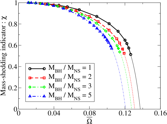
Figure 6: Extrapolation of sequences with $\mathcal{C}=0.145$ to the mass-shedding limit, $\mathcal{X}=0$. The thick curves are sequences constructed using numerical data, and the thin curves are their extrapolations. The horizontal axis is the orbital angular velocity in the polytropic unit, $\bar{\Omega}=\Omega R_{\mathrm{poly}}[=\Omega R_{\mathrm{poly}}/c]$. Image reproduced with permission from Taniguchi et al. (2008), copyright by APS.

Taniguchi et al. (2008) tabulated the values of $\mathcal{X}$ as a function of the orbital angular velocity and their sequence is extrapolated to $\mathcal{X}=0$ by using polynomial functions to find the orbits at the onset of mass shedding. Figure 6 shows an example of such extrapolations for sequences with $\mathcal{C}=0.145$ and $Q=1,2,3,$ and $5$. By extrapolating results toward $\mathcal{X}=0$, the orbital angular velocity at the mass-shedding limit, $\Omega_{\mathrm{ms}}$, is approximately determined for each set of $Q$ and $\mathcal{C}$.

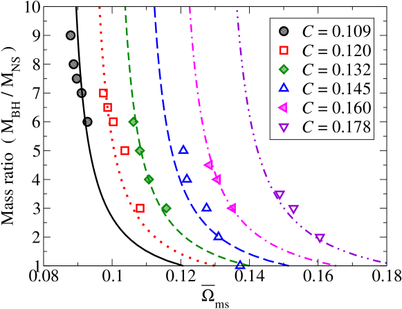
Figure 7: Fit of the mass-shedding limit by the analytic expression, Eq. (30). The mass-shedding limit for each compactness of the neutron star and mass ratio is computed by extrapolating the numerical data. Image reproduced with permission from Taniguchi et al. (2008), copyright by APS.

To derive a fitting formula for $\Omega_{\mathrm{ms}}$ as a function of $Q$ and $\mathcal{C}$, the Newtonian expression of Eq. (11) is useful, although it is semiquantitative. By fitting the sequence of data with respect to this expression, Taniguchi et al. (2008) determined the value of $C_{\Omega}$ for the $\Gamma=2$ polytrope to be $0.270$, i.e.,

$$\bar{\Omega}_{\mathrm{ms}}=0.270\frac{\mathcal{C}^{3/2}}{\bar{M}_{\mathrm{NS}}}\pqty{1+Q^{-1}}^{1/2},$$ (30)

or equivalently,

$$\Omega_{\mathrm{ms}}m_{0}=0.270\mathcal{C}^{3/2}(1+Q)\pqty{1+Q^{-1}}^{1/2}.$$ (31)

Figure 7 shows the results of the fitting for the mass-shedding limit. The agreement is not perfect but fairly good for $Q\geq 2$.

It may be interesting to note that the value of $C_{\Omega}=0.270$ is the same as that found for quasiequilibrium sequences in general relativity of binary neutron stars (Taniguchi and Shibata, 2010) and of black hole–corotating neutron star binaries (Shibata and Uryū, 2006, 2007). Thus, the value of $C_{\Omega}=0.270$ could be widely used for an estimation of the orbital angular velocity at the mass-shedding limit of a neutron star in a relativistic binary system with $\Gamma=2$. We also note that $C_{\Omega}=0.270$ corresponds to $c_{\mathrm{R}}=1.90$, which is defined in Sect. 1.3.1.

2.4.2 Innermost stable circular orbit

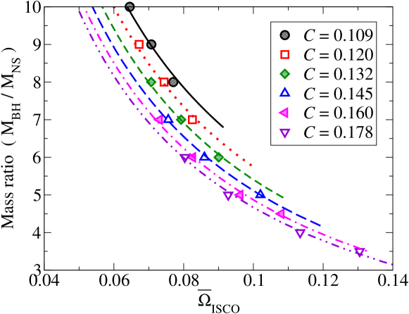
Figure 8: Fit of the minimum point of the binding energy curve by Eq. (33). Image reproduced with permission from Taniguchi et al. (2008), copyright by APS.

Next, we summarize the results for the orbital angular velocity at which the minimum of the binding energy, i.e., the innermost stable circular orbit appears. Because the numerical data are discrete and do not necessarily give the exact minimum, the minimum point may be located approximately by fitting three nearby points of the sequence to a second-order polynomial.

A simple empirical fitting that predicts the angular velocity $\Omega_{\mathrm{ISCO}}$ at the innermost stable circular orbit for an arbitrary companion orbiting a black hole may be derived in the manner of Taniguchi et al. (2008). They search for an expression of $\Omega_{\mathrm{ISCO}}$ as a function of the mass ratio $Q$ and the compactness $\mathcal{C}$ of the companion. Specifically, they assume a functional form of

$$\Omega_{\mathrm{ISCO}}m_{0}=c_{1}\bqty{1-\frac{c_{2}}{Q^{p_{1}}}\pqty{1-c_{3}\mathcal{C}^{p_{2}}}},$$ (32)

where $c_{1}$, $c_{2}$, $c_{3}$, $p_{1}$, and $p_{2}$ are parameters to be determined in the following manner. The coefficients $c_{1}$, $c_{2}$, and $c_{3}$ are determined for given values of $p_{1}$ and $p_{2}$ by requiring that three known values of $\Omega_{\mathrm{ISCO}}$ are recovered: (1) that of a test particle orbiting a Schwarzschild black hole, $\Omega_{\mathrm{ISCO}}m_{0}=6^{-3/2}$ (for $Q\to\infty$), (2) that of an equal-mass binary-black-hole system, $\Omega_{\mathrm{ISCO}}m_{0}=0.1227$ (for $Q=1$ and $\mathcal{C}=0.5$; Caudill et al., 2006), and finally (3) that of a black hole–neutron star configuration with $Q=5$ and $\mathcal{C}=0.1452$, $\Omega_{\mathrm{ISCO}}m_{0}=0.0854$ (Taniguchi et al., 2008). The exponents $p_{1}$ and $p_{2}$ are determined by requiring the fitted curves to lie near the data points for all the systems.

As demonstrated in Fig. 8, the numerical data are fitted nicely by a function

$$\Omega_{\mathrm{ISCO}}m_{0}=0.0680\bqty{1-\frac{0.444}{Q^{0.25}}\pqty{1-3.54\mathcal{C}^{1/3}}}.$$ (33)

The agreement is sufficient for finding the orbital angular velocity at the innermost stable circular orbit within the error of $\sim 10\%$.

2.4.3 Critical mass ratio

Figure 9: Example of the boundary between the mass-shedding limit and the innermost stable circular orbit for $\mathcal{C}=0.145$. The solid and dashed curves denote the mass ratio that gives the mass-shedding limit and the innermost stable circular orbit (ISCO), respectively, for a given value of the orbital angular velocity in the polytropic unit. The thin dotted curve denotes the mass-shedding limit for unstable quasiequilibrium sequences. Image reproduced with permission from Taniguchi et al. (2008), copyright by APS.

Combining Eqs. (31) and (33), we can identify the critical binary parameters which separate two final fates that the binary encounters an innermost stable circular orbit before initiating mass shedding or that the neutron star reaches the mass-shedding limit before plunging into the black hole. Figure 9 illustrates the final fate of black hole–neutron star binaries with $\mathcal{C}=0.145$. Because the orbital angular velocities at the mass-shedding limit [Eq. (31)] and the innermost stable circular orbit [Eq. (33)] depend differently on the mass ratio, $Q$, they intersect in this figure. An inspiraling binary evolves along horizontal lines toward increasing $\bar{\Omega}$, i.e., from the left to the right, until it reaches either the innermost stable circular orbit or the mass-shedding limit. For a sufficiently high mass ratio, the binary reaches an innermost stable circular orbit. Quasiequilibrium sequences cannot predict the fate of the neutron star after that, because it enters a dynamical plunge phase (see Sect. 3). Thus, the mass-shedding limit for unstable quasiequilibrium sequences included in Fig. 9 should be regarded as only indicative. As shown in Fig. 9, the sequence with $Q=6$ (dot-dashed line) encounters the innermost stable circular orbit, while that with $Q=3$ (dot-dot-dashed line) ends at the mass-shedding limit. The intersection of the curve for the mass-shedding limit and that for the innermost stable circular orbit marks a critical point that separates the two distinct fates of the binary inspiral. Specifically, the critical mass ratio is found to be $Q\approx 4.2$ for this case, i.e., binaries of a nonspinning black hole and an irrotational neutron star with $\mathcal{C}=0.145$ modeled by a $\Gamma=2$ polytrope.

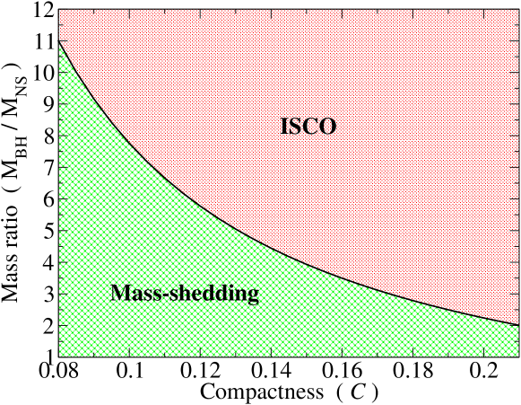
Figure 10: Critical mass ratio which separates black hole–neutron star binaries that encounter an innermost stable circular orbit before initiating mass shedding and those undergoing tidal disruption, as a function of the compactness of the neutron star modeled by the $\Gamma=2$ polytrope. As we discuss in Sect. 3, while configurations in “ISCO” nearly certainly end up in the plunge without tidal disruption, only a part of configurations in “Mass-shedding” leads to appreciable tidal disruption. Image reproduced with permission from Taniguchi et al. (2008), copyright by APS.

The critical mass ratio which separates black hole–neutron star binaries that encounter an innermost stable circular orbit before initiating mass shedding and those reach the mass-shedding limit before the plunge is obtained as a function of the compactness of the neutron star by equating Eqs. (31) and (33). Specifically, the critical mass ratio is determined by

$$0.270\mathcal{C}^{3/2}(1+Q)\pqty{1+Q^{-1}}^{1/2}=0.0680\bqty{1-\frac{0.444}{Q^{0.25}}\pqty{1-3.54\mathcal{C}^{1/3}}},$$ (34)

and the curve that separates those two regions on the $Q$-$\mathcal{C}$ plane is shown in Fig. 10. If the mass ratio of a black hole–neutron star binary is higher than the critical value, the quasiequilibrium sequence terminates by encountering the innermost stable circular orbit, while if lower, it ends at the mass-shedding limit. We emphasize that the mass shedding is only a necessary condition for tidal disruption. In Sect. 3, we will see that dynamical simulations tend to predict that tidal disruption occurs for a more restricted range of parameters than that shown in Fig. 10.

We again caution that the classification shown in Fig. 10 is appropriate only for nonspinning black hole–neutron star binaries. The spin of the black hole significantly modifies the critical mass ratio. For example, if the spin of the black hole is high and prograde, i.e., aligned with the orbital angular momentum of the binary, the region of “Mass-shedding” will be enlarged significantly. Systematic studies on the effect of black-hole spins have not been performed yet, and further investigations are awaited.

2.5 Summary and issues for the future

In this section, we have reviewed the current status of the studies on quasiequilibrium sequences of black hole–neutron star binaries in general relativity, focusing mainly on Taniguchi et al. (2008). In particular, we highlighted a curve of the critical mass ratio, which separates black hole–neutron star binaries that encounter an innermost stable circular orbit before initiating mass shedding and vice versa, as a function of the compactness of the neutron star. The result is shown in Eq. (34) and in Fig. 10. Such a critical curve clearly classifies the possible final fate of black hole–neutron star binaries, which depends on the mass ratio and the compactness of the neutron star for a given equation of state. The final fate depends also on the spin of the black hole (see Sect. 3), although only nonspinning configurations are discussed here.

As seen in Table 2, the parameter space surveyed is still quite narrow, partly because the community has been devoting effort to dynamical simulations. A systematic study of quasiequilibrium sequences has been done only for binaries composed of a nonspinning black hole and an irrotational neutron star with the $\Gamma=2$ polytrope. It may be useful to survey the remaining parameter space in a systematic manner in the future. Systematic numerical results for such a study will be helpful for predicting the final fate of black hole–neutron star binaries and for checking the results derived in numerical simulations in light of the high computational precision of quasiequilibrium states. Specifically, quasiequilibrium sequences of binaries composed of a spinning black hole and a neutron star with an equation of state other than the $\Gamma=2$ polytrope remain to be studied in detail.

The formulation for quasiequilibrium states should be improved further for more rigorous studies. To date, all the computations adopted formulations which solve only five out of ten components of the Einstein equation: constraint equations and the slicing condition (see Appendix A). Employing an improved formulation in which full components of the Einstein equation are solved is left for the future (see Shibata et al. 2004; Cook and Baumgarte 2008 for proposed formulations and Uryū et al. 2006, 2009 for studies of binary neutron stars).

3 Merger and postmerger simulation

Dynamical simulations for coalescences of black hole–neutron star binaries have been performed in full general relativity by several groups since Shibata and Uryū (2006). These studies have explored the merger process, the criterion for tidal disruption of a neutron star, the mass and the spin parameter of the remnant black hole, properties of the remnant disk and the ejected material, and gravitational waveforms. Results from different groups agree with each other quantitatively when they can be compared. Longterm simulations of the accretion disks around black holes for $\sim$10\text{\,}\mathrm{s}$$ are also becoming available in recent years. These studies begin to clarify the evolution of the dense and hot accretion disk, neutrino luminosity, the role of neutrino emission, properties of the disk outflow, and possible launch of an ultrarelativistic jet. In this section, we review our current understanding about these topics.

3.1 Numerical method for coalescence simulations

Numerical-relativity simulations for black hole–neutron star binary coalescences are performed by solving the Einstein evolution equations with appropriate gauge conditions and hydrodynamics equations, which may involve neutrino-radiation transfer and magnetohydrodynamics. General formulation and numerical techniques are summarized in Appendix B. In this Sect. 3.1, we summarize general aspects of initial data and equations of state adopted in numerical simulations of black hole–neutron star binary coalescences.

Numerical-relativity simulations for black hole–neutron star binaries throughout the inspiral-merger-postmerger phases have typically been performed only for $\lesssim$100\text{\,}\mathrm{ms}$$ and are still in the early stage for studying the postmerger evolution. To explore the longterm evolution of the merger remnant, simulations of black hole–accretion disk systems have also been performed in full general relativity for $\gtrsim$1\text{\,}\mathrm{s}$$ (Fujibayashi et al., 2020a, b, see also Most et al. 2021b). The setup of these simulations will be described separately in Sect. 3.5.

3.1.1 Initial condition

Realistic simulations of black hole–neutron star binary coalescences always adopt quasiequilibrium states reviewed in Sect. 2 as their initial conditions. Typically, simulations based on the generalized harmonic formalism with the excision method adopt quasiequilibrium states computed in the excision framework. While many simulations based on the BSSN formalism (or its extension) with the moving-puncture method adopt quasiequilibrium states computed in the puncture framework, quasiequilibrium states computed in the excision framework have also been adopted (Etienne et al., 2008, 2009, 2012a, 2012c; Paschalidis et al., 2015; Ruiz et al., 2018, 2020; Most et al., 2021a). Because the moving-puncture method needs data of the metric inside the excision surface in the initial configurations, the interior needs to be filled artificially by extrapolating the data outside the excision surface. This extrapolation generally produces constraint-violating initial data, and care must be taken so that this violation does not affect significantly the evolution outside the excision surface (Etienne et al., 2007, see also Brown et al. 2007).

Strictly speaking, quasiequilibrium states derived under the assumption of the helical symmetry cannot be realistic, because the radial approaching velocity induced by gravitational radiation reaction is not taken into account. This drawback gives rise to the inspiral motion with the residual eccentricity of $e\gtrsim 0.01$ for typical initial data. Because the eccentricity of $e\approx 0.01$ introduces a phase shift larger than the tidal effect (Favata, 2014), numerical simulations used for developing theoretical templates are required to adopt initial data with the eccentricity as low as $e\lesssim${10}^{-3}$$ in order not to bias estimation of tidal deformability in the analysis of gravitational waves from realistic circular binaries. Although the residual eccentricity may be reduced if we could start simulations from a distant orbit at which radiation reaction is sufficiently weak, this is not practical with current and near-future computational resources. To obtain low-eccentricity inspirals with a reasonable initial separation, iterative eccentricity reduction is routinely applied in the excision-based simulations (Foucart et al., 2008, see Appendix A.5.2 for details). Essentially the same technique has recently been developed for and applied to puncture-based initial data (Kyutoku et al., 2021).

Because all the quasiequilibrium states have been computed in the framework of pure ideal hydrodynamics assuming that the neutron star is cold, additional variables need to be specified if we perform simulations with detailed microphysics. For evolving neutron stars with composition-dependent equations of state, we need to give the electron fraction in the initial condition. These variables are usually determined by the condition of a(n approximate) zero-temperature $\beta$-equilibrium (see, e.g., Duez et al., 2010). This step is in particular necessary for neutrino-radiation-hydrodynamics simulations (Deaton et al., 2013; Foucart et al., 2014, 2017; Brege et al., 2018; Kyutoku et al., 2018; Foucart et al., 2019b; Most et al., 2021a).

For magnetohydrodynamics simulations, magnetic fields are superposed on the initial configuration with arbitrary strength and arbitrary geometry. Their magnitude should not be very large, because too strong magnetic fields destroy the hydrostationary equilibrium. Still, this condition admits an astrophysically strong magnetic fields of $\lesssim${10}^{17}\text{\,}\mathrm{G}$$ in the neutron star, for which the gravitational binding energy is larger by orders of magnitude. To resolve short-wavelength modes associated with the magnetorotational instability in the postmerger phase (Balbus and Hawley, 1991), it is customary to impose magnetar-level magnetic fields inside neutron stars. This may be justified, because the magnetic fields are likely to be amplified on a dynamical time scale in the accretion disk formed after merger in the real world. However, it has not been clarified yet whether a strong and coherent poloidal field is really established by some mechanism, e.g., the dynamo process. While many magnetohydrodynamics simulations have adopted poloidal magnetic fields initially confined in the neutron star to avoid difficulty in handling force-free magnetospheres (Chawla et al., 2010; Etienne et al., 2012a, c; Kiuchi et al., 2015b; Most et al., 2021a), pulsar-like dipolar magnetic fields are also adopted with a non-tenuous artificial atmosphere outside the neutron star in simulations that focus on the possible jet launch (Paschalidis et al., 2015; Ruiz et al., 2018, 2020). We note that an artificial atmosphere itself is always required by hydrodynamics simulations performed in a conservative scheme (see also Appendix B.2.2).

3.1.2 Equation of state

The equation of state for neutron-star matter is a key ingredient for deriving realistic outcomes of and multimessenger signals from black hole–neutron star binary coalescences. The primary reason for this is that the equation of state determines the density distribution and hence the radius of the neutron star for a given value of the mass. Whether tidal disruption occurs or not during the coalescence and, if it occurs, its degree are determined primarily by the radius or the compactness of the neutron star for given masses and spins of binary components [see Eq. (34)]. Thus, the gravitational waveform, the properties of the remnant disk, and the properties of the ejecta are governed crucially by the equation of state. The equation of state also determines the tidal deformability of the neutron star, which affects the late inspiral phase of compact binary coalescences.

However, as mentioned in Sect. 2.1.2, the equation of state for supranuclear-density matter is still uncertain (see, e.g., Lattimer and Prakash 2016; Oertel et al. 2017; Baym et al. 2018 for reviews). In the study of compact binary coalescences involving neutron stars, it is more beneficial to explore the possibility of determining the equation of state via gravitational-wave observations (Lindblom, 1992; Vallisneri, 2000; Read et al., 2009b; Ferrari et al., 2010; Lackey et al., 2012; Maselli et al., 2013; Lackey et al., 2014; Pannarale et al., 2015b) than to derive observable signals relying on a single candidate of the realistic equation of state. For this purpose, it is necessary to prepare theoretical templates of gravitational waveforms by performing simulations systematically over the parameter space of black hole–neutron star binaries with a wide variety of hypothetical equations of state. Such a systematic survey is also indispensable for predicting electromagnetic counterparts (see Sect. 3.4 for the dependence of the disk and ejecta properties on the equation of state). Thus, all the equations of state adopted in simulations reviewed in this article should be understood as hypothetical.

Due to the reason described in Sect. 2.1.2, we may safely adopt zero-temperature equations of state during the inspiral and early merger phases before the shock heating begins to play a role. Moreover, the zero-temperature equations of state are sufficient for simulating black hole–neutron star binary coalescences which do not result in tidal disruption of neutron stars, because essentially no heating process is involved. However, because polytropes are not quantitative models of neutron stars, it is desirable to adopt nuclear-theory-based equations of state for the purpose of investigating realistic black hole–neutron star binary coalescences.

Sophisticated zero-temperature equations of state are implemented in numerical simulations by various means. A straightforward method is to adopt numerical tables calculated based on hypothetical models of nuclear physics (see, e.g., Glendenning and Moszkowski, 1991; Müller and Serot, 1996; Akmal et al., 1998; Douchin and Haensel, 2001; Alford et al., 2005). The drawback of this method is that the capability of systematic studies is limited by available tables. A popular tool for conducting a systematic study is an analytic, piecewise-polytropic equation of state, with which the pressure is given by a broken power-law function of the rest-mass density as

$$P(\rho)=\kappa_{i}\rho^{\Gamma_{i}}\;(\rho_{i}\leq\rho<\rho_{i+1}),$$ (35)

where $i\in[0:n-1]$, $\rho_{0}=0$, and $\rho_{n}\to\infty$ (Read et al., 2009b, a; Özel and Psaltis, 2009, see also O’Boyle et al. 2020 for generalization and Haensel and Potekhin 2004; Lindblom 2010; Potekhin et al. 2013 for other analytic approaches). It has been shown that most of the nuclear-theory-based equations of state for neutron-star matter can be approximated to reasonable accuracy up to the rest-mass density of $\gtrsim${10}^{15}\text{\,}\mathrm{g}\text{\,}{\mathrm{cm}}^{-3}$$ by piecewise polytropes consisting of one for the crust region and three for the core region if we choose $\rho_{2}=$e14.7\text{\,}\mathrm{g}\text{\,}{\mathrm{cm}}^{-3}$$ and $\rho_{3}=${10}^{15}\text{\,}\mathrm{g}\text{\,}{\mathrm{cm}}^{-3}$$ (Read et al., 2009a).

It is remarkable that the maximum density in the system only decreases in time (except for possible minor fluctuations) during the black hole–neutron star binary coalescences. This is a striking difference from the binary-neutron-star merger, after which a massive or collapsing neutron star with increased central density is formed (see, e.g., Hotokezaka et al., 2011; Takami et al., 2015; Dietrich et al., 2015; Foucart et al., 2016a). This property indicates that black hole–neutron star binaries are not influenced by the equation of state at very high density, e.g., several times the nuclear saturation density, unless the neutron star is close to the maximum-mass configuration. Thus, numerical simulations for binaries with plausibly canonical $\sim 1.4\,M_{\odot}$ neutron stars may safely adopt simplified models of nuclear-matter equations of state. For example, if the central density is lower than ${10}^{15}\text{\,}\mathrm{g}\text{\,}{\mathrm{cm}}^{-3}$, we may adopt piecewise polytropes with a reduced number of pieces for the core focusing only on its low-density part (Read et al., 2009b; Kyutoku et al., 2010, 2011a). This feature also indicates a weak point that we will not be able to investigate properties of ultrahigh-density matter from observations of black hole–neutron star binaries without extrapolation relying on theoretical models (see, e.g., Abbott et al., 2018; Raaijmakers et al., 2019).

Once the heating process is activated in the merger phase, particularly via the shock associated with self-crossing of the tidal tail, the zero-temperature approximation is no longer valid. Finite-temperature effects become increasingly important in the remnant disk, because temperature increases due to the shock interaction and presumably to subsequent viscous heating associated with magnetohydrodynamical turbulence, while the Fermi energy decreases due to the decreased rest-mass density compared to neutron stars.

One popular and qualitative approach for incorporating finite-temperature effects is to supplement zero-temperature equations of state with an approximate correction. A simple prescription for this purpose is to add an ideal-gas-like term (Janka et al., 1993),

$$P_{\mathrm{th}}=(\Gamma_{\mathrm{th}}-1)\rho\varepsilon_{\mathrm{th}},$$ (36)

where $\varepsilon_{\mathrm{th}}(\varepsilon,\rho):=\varepsilon-\varepsilon_{\mathrm{cold}}(\rho)$ is the finite-temperature part of the specific internal energy with $\varepsilon_{\mathrm{cold}}(\rho)$ being the specific internal energy given by a zero-temperature equation of state. Indeed, the ideal-gas equation of state, $P=(\Gamma-1)\rho\varepsilon$, which reduces to a polytrope with the adiabatic index $\Gamma$ for the isentropic fluid and/or at zero temperature assumed in computations of quasiequilibrium, is occasionally adopted in dynamical simulations as a qualitative model of neutron-star matter. A parameter $\Gamma_{\mathrm{th}}$ represents the strength of the thermal effect, and its appropriate value may be estimated by calibration with simulations performed adopting genuinely finite-temperature equations of state, which are usually given by numerical tables (Bauswein et al., 2010; Figura et al., 2020). It should be cautioned that, however, the constant value of $\Gamma_{\mathrm{th}}$ is not faithful to nuclear-theory-based calculations (Constantinou et al., 2015) even though uncertain thermal effects at supranuclear density may not be relevant to black hole–neutron star binary coalescences (Carbone and Schwenk, 2019). In addition, the use of zero-temperature equations of state is not fully justified after tidal disruption even if the temperature is not increased. This is because, although zero-temperature equations of state are derived as a function of a single variable, e.g., rest-mass density, assuming the $\beta$-equilibrium, the rapid decompression of the disrupted material preserves the composition on a dynamical time scale and violates the $\beta$-equilibrium condition (Foucart et al., 2017).

To investigate the entire merger and postmerger phases in a self-consistent manner, it is necessary to adopt temperature- and composition-dependent equations of state with an appropriate scheme for neutrino transport (see Appendix B.2.1). These equations of state are usually given in a tabulated form as e.g.,

$$P =P(\rho,T,Y_{\mathrm{e}}),$$ (37)

$$\varepsilon =\varepsilon(\rho,T,Y_{\mathrm{e}}),$$ (38)

where $T$ and $Y_{\mathrm{e}}$ are the temperature and the electron fraction, respectively (see, e.g., Lattimer and Swesty, 1991; Shen et al., 1998; Hempel et al., 2012; Steiner et al., 2013; Banik et al., 2014, see also Raithel et al. 2019 for a detailed analytic approach to augment zero-temperature equations of state in a similar manner to Eq. (36)). Because these variables are tightly related to neutrino emission and absorption, neutrino transport is an essential ingredient for accurately determining thermal properties of material in the postmerger phase. Multidimensional neutrino-radiation-hydrodynamics simulations in full general relativity have been developed in the stellar-core collapse (Sekiguchi, 2010; Sekiguchi and Shibata, 2011) and are later applied to binary neutron stars (Sekiguchi et al., 2011b, a) as well as black hole–neutron star binaries (Deaton et al., 2013; Foucart et al., 2014; Kyutoku et al., 2018).

3.2 Current parameter space surveyed

As reviewed in Sect. 2.1, models of black hole–neutron star binaries are characterized by various parameters. In this section, we focus only on the models in which neutron stars are initially in the irrotational state, which is presumably realistic for the majority of compact object binaries as we discussed in Sect. 1.2 (see Foucart et al. 2019a; Ruiz et al. 2020 for studies on spinning neutron stars). Then, the properties of binaries are characterized by the mass of the black hole, $M_{\mathrm{BH}}$, the spin parameter of the black hole, $\chi$, its orientation, $\iota$, and the mass of the neutron star, $M_{\mathrm{NS}}$. Furthermore, hypothetical equations of state for neutron-star matter should also be regarded as a free parameter (or function) characterizing the models. Properties of an equation of state may be usefully represented by the radius of the neutron star, $R_{\mathrm{NS}}$, particularly when we focus on tidal disruption.

To date, numerical-relativity simulations of black hole-neutron star binaries have been performed focusing mainly on neutron stars with typical masses in our Galaxy of $M_{\mathrm{NS}}\approx 1.2$–$1.5\,M_{\odot}$ (Tauris et al., 2017; Farrow et al., 2019). Accordingly, the results are reviewed below focusing on the models with these typical values. Because the mass of the neutron star does not vary much among the models, it is useful in many occasions to characterize a binary model by quantities directly related to the criterion for mass shedding to occur outside the innermost stable circular orbit, Eq. (9), namely the mass ratio $Q$ and the compactness $\mathcal{C}$ instead of $M_{\mathrm{BH}}$ and $R_{\mathrm{NS}}$, respectively. This parametrization is also sufficient for qualitative but scale-free polytropic equations of state (see Sect. 2.3). It will be worthwhile in the future to simulate mergers of black hole–neutron star binaries with $M_{\mathrm{NS}}\sim 2\,M_{\odot}$ employing nuclear-theory-based equations of state, particularly in light of possible detections of such neutron stars with gravitational waves (Abbott et al., 2020a, 2021b), although tidal disruption is unlikely to be common due to the large compactness (see also Sect. 4.2.1).

The range of the mass ratio covered by numerical-relativity simulations has been enlarged to $1\leq Q\lesssim 8.3$ in the last decade. The small value in this range is adopted to clarify the difference between black hole–neutron star binaries and binary neutron stars in the feature of the mergers, and we will discuss this topic in Sect. 4.2.2. The large values of $Q$ are directly related to realistic black hole–neutron star binaries, taking into account the fact that the observed stellar-mass black holes typically have $M_{\mathrm{BH}}\gtrsim 5$–$7\,M_{\odot}$ (Özel et al., 2010; Kreidberg et al., 2012; Abbott et al., 2019a, 2021a, see also Thompson et al. 2019 for a low-mass black-hole candidate with $\sim 3.3^{+2.8}_{-0.7}\,M_{\odot}$).

A wide range of black-hole spins, both in terms of the magnitude and the orientation, have been adopted in simulations of black hole–neutron star binaries. Most of the recent simulations have focused on the prograde spin, because it is required for tidal disruption by massive black holes with $M_{\mathrm{BH}}\gtrsim 5\,M_{\odot}$ or $Q\gtrsim 4$. Notably, the largest value of the spin parameter simulated is increased to $\chi=0.97$ (Lovelace et al., 2013). Although this is only the case for a single system with $Q=3$, the capability of simulating nearly-extremal black holes is important for future investigations of tidal disruption in high mass-ratio systems. Inclined spins of the black holes are also handled in many simulations. Essentially all the orientations of the spin have already been handled, although covering the parameter space becomes computationally demanding simply because of the increased degree of freedom.

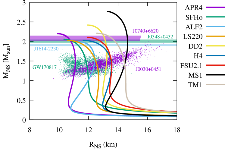
Figure 11: Mass-to-radius relation of cold, spherical neutron stars for various equations of state. Unstable configurations with small radii are not shown in this plot. We also display the measured mass (68.3% credibility) of a pulsar in J1614-2230 (cyan band: Demorest et al., 2010; Arzoumanian et al., 2018), that in J0348+0432 (green band: Antoniadis et al., 2013), that in J0740+6620 (magenta band: Cromartie et al., 2020; Fonseca et al., 2021), posterior samples obtained by analysis of J0030+0451 (magenta dot: Miller et al., 2019b, thinned out from provided samples), and those by analysis of GW170817 (green dot: Abbott et al., 2018).

Table 3: List of representative equations of state adopted in simulations of black hole–neutron star binary coalescences and characteristic quantities of neutron stars. $M_{\mathrm{max}}$ denotes the maximum mass of cold, spherical neutron stars. $M_{\mathrm{B},1.35}$, $R_{1.35}$, $\mathcal{C}_{1.35}$, and $\Lambda_{1.35}$ are, respectively, the baryon rest mass, the circumferential radius, the compactness, and the $l=2$ tidal deformability of a $1.35\,M_{\odot}$ neutron star.

Name	Reference	$M_{\mathrm{max}}[\,M_{\odot}]$	$M_{\mathrm{B},1.35}[\,M_{\odot}]$	$R_{1.35}($\mathrm{km}$)$	$\mathcal{C}_{1.35}$	$\Lambda_{1.35}$
APR4	Akmal et al. (1998)	$2.20$	$1.50$	$11.1$	$0.180$	$322$
SFHo	Steiner et al. (2013)	$2.06$	$1.48$	$11.9$	$0.167$	$420$
ALF2	Alford et al. (2005)	$1.99$	$1.49$	$12.4$	$0.161$	$733$
LS220	Lattimer and Swesty (1991)	$2.03$	$1.48$	$12.6$	$0.158$	$653$
DD2	Banik et al. (2014)	$2.42$	$1.47$	$13.2$	$0.151$	$854$
H4	Lackey et al. (2006)	$2.03$	$1.47$	$13.6$	$0.147$	$1110$
FSU2.1	Shen et al. (2011)	$2.10$	$1.46$	$13.6$	$0.147$	$980$
MS1	Müller and Serot (1996)	$2.77$	$1.46$	$14.4$	$0.138$	$1740$
TM1	Hempel et al. (2012)	$2.21$	$1.46$	$14.5$	$0.138$	$1430$

After the early days of adopting qualitative ideal-gas (polytropic at zero temperature) equations of state, many simulations have been performed with nuclear-theory-based equations of state. In particular, temperature- and composition-dependent equations of state are routinely adopted in neutrino-radiation-hydrodynamics numerical-relativity simulations. Figure 11 shows the mass-to-radius relations of neutron stars for various equations of state which are popular in numerical-relativity simulations, along with constraints on the neutron-star properties derived by observations of Galactic massive pulsars (Demorest et al., 2010; Antoniadis et al., 2013; Arzoumanian et al., 2018; Cromartie et al., 2020; Fonseca et al., 2021), J0030+0451 by NICER (Miller et al., 2019b), and GW170817 by the LIGO-Virgo collaboration (Abbott et al., 2018). Table 3 summarizes characteristic quantities of neutron stars modeled by these equations of state. Because the maximum mass of the neutron star is widely accepted to exceed $\sim 2\,M_{\odot}$ from the observations of massive pulsars, recent numerical simulations seldom employ soft equations of state which are incompatible with these measurements.

Last but not least, various magnetohydrodynamics simulations have been performed. It should be cautioned that the initial strength and geometry of magnetic fields need to be chosen somewhat arbitrarily in current simulations (see Sect. 3.5.3). This limitation might not affect the numerical evolution of the remnant accretion disk if the grid resolution is sufficiently high. This is because the magnetic fields inside the accretion disk are expected to be amplified by the magnetorotational instability and a turbulent state is expected to be developed (see, e.g., Balbus and Hawley 1998 for reviews). Consequently, the relaxed quasisteady state should not depend on the initial conditions. However, the grid resolution is usually not high enough for guaranteeing numerical convergence due to the limited computational resources. Thus, results obtained by current magnetohydrodynamics simulations should be carefully interpreted. We also caution that the global configuration of the magnetic field in the final state could be impacted by the initial choice of a large-scale poloidal field.

3.3 Merger process

We begin with the review of the merger process focusing on tidal disruption, subsequent disk formation, and dynamical mass ejection (or absence thereof). In particular, this Sect. 3.3 focuses on the dynamics until $\sim$10\text{\,}\mathrm{ms}$$ after the onset of merger. Effects of the magnetic field (Chawla et al., 2010; Etienne et al., 2012a, c; Kiuchi et al., 2015b) and/or neutrino transport (Deaton et al., 2013; Foucart et al., 2014; Kyutoku et al., 2018) play a significant role in the dynamical evolution of the system only after the disrupted material winds around the black hole and collides itself to form a circularized disk. Thus, properties of the neutron star are characterized only by the mass and zero-temperature equations of state during the processes discussed here.

The orbital separation of a black hole–neutron star binary decreases due to dissipation of the energy and the angular momentum via gravitational radiation reaction, and eventually two objects merge. As we discussed in Sect. 1, the final fate of black hole–neutron star binary coalescences is classified into two categories (we will later refine this dichotomy). One is the case in which the neutron star is swallowed by the black hole without experiencing tidal disruption. The other is the case in which the neutron star is tidally disrupted outside the innermost stable circular orbit of the black hole. As we described in Sect. 1.3.1, which of these two possibilities is realized is determined primarily by competition between the orbital separation at which the tidal disruption occurs and the radius of the innermost stable circular orbit. Figures 12 and 13 display the snapshots of the rest-mass density and the region inside the apparent horizon on the equatorial plane at selected time slices for typical examples of these two categories (Kyutoku et al., 2015).

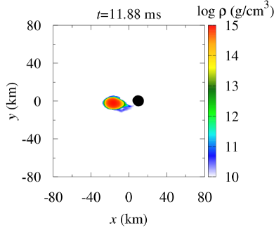
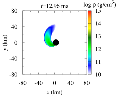
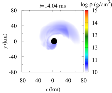
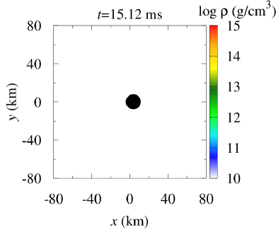
Figure 12: Evolution of the rest-mass density profile and the location of the apparent horizon on the equatorial plane for a binary with $M_{\mathrm{BH}}=4.05\,M_{\odot}$, $\chi=0$, $M_{\mathrm{NS}}=1.35M_{\odot}$, and $R_{\mathrm{NS}}=$11.1\text{\,}\mathrm{km}$$ ($Q=3$, $\mathcal{C}=0.180$) modeled by a piecewise-polytropic approximation of the APR4 equation of state (Akmal et al., 1998). The black filled circles denote the regions inside the apparent horizon of the black hole. The color map of each figure shows $\log_{10}(\rho[$\mathrm{g}\text{\,}{\mathrm{cm}}^{-3}$])$. This figure is generated from data of Kyutoku et al. (2015).

Figure 12 illustrates the case in which the neutron star is not tidally disrupted before it is swallowed by the black hole. This system is characterized by $M_{\mathrm{BH}}=4.05\,M_{\odot}$, $\chi=0$, $M_{\mathrm{NS}}=1.35\,M_{\odot}$, and $R_{\mathrm{NS}}=$11.1\text{\,}\mathrm{km}$$ ($Q=3$, $\mathcal{C}=0.180$) modeled by a piecewise-polytropic approximation of the APR4 equation of state (Akmal et al., 1998). Because the neutron star is tidally deformed significantly only after it comes very close to the black hole, mass shedding sets in for an orbit too close to induce subsequent disruption outside the innermost stable circular orbit. This is consistent with the expectation from Fig. 10 presented in Sect. 2.4. Accordingly, the masses of the remnant disk and the dynamical ejecta are negligible, say, $\ll 0.01\,M_{\odot}$. At the same time, most of the neutron-star material falls into the black hole approximately simultaneously through a narrow region of the horizon. This coherent infall efficiently excites quasinormal-mode oscillations of the remnant black hole. We discuss gravitational waves later in Sect. 3.6. Overall, the behavior of the system in this category universally resembles that of binary-black-hole coalescences with the same masses and spins of components, because the finite-size effect of the neutron star does not play a role (Foucart et al., 2013a). This seems to be the case for all the black hole–neutron star binaries and their candidates reported as of 2021 (Abbott et al., 2021a, b).

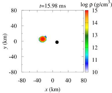
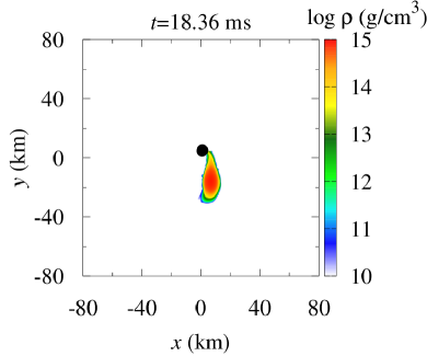
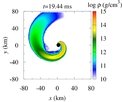
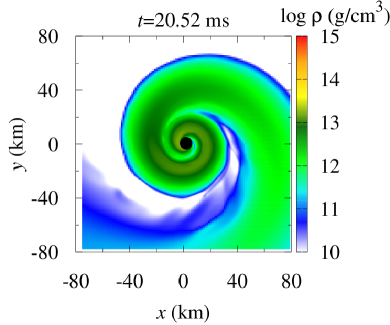
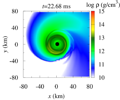
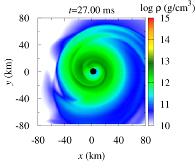
Figure 13: Same as Fig. 12 but for a binary with $M_{\mathrm{BH}}=4.05M_{\odot}$, $\chi=0.75$, $M_{\mathrm{NS}}=1.35\,M_{\odot}$, and $R_{\mathrm{NS}}=$11.1\text{\,}\mathrm{km}$$ ($Q=3$, $\mathcal{C}=0.180$) modeled by a piecewise-polytropic approximation of the APR4 equation of state (Akmal et al., 1998). This figure is generated from data of Kyutoku et al. (2015).

Figure 13 illustrates the case in which the neutron star is disrupted before the binary reaches the innermost stable circular orbit. This system is characterized by $M_{\mathrm{BH}}=4.05\,M_{\odot}$, $\chi=0.75$, $M_{\mathrm{NS}}=1.35\,M_{\odot}$, and $R_{\mathrm{NS}}=$11.1\text{\,}\mathrm{km}$$ ($Q=3$, $\mathcal{C}=0.180$) modeled by a piecewise-polytropic approximation of the APR4 equation of state (Akmal et al., 1998). In this case, mass shedding from an inner cusp of the deformed neutron star sets in at an orbital separation much larger than that of the innermost stable circular orbit. After a substantial amount of material is removed from the inner cusp, the neutron star is tidally disrupted outside the innermost stable circular orbit. It should be emphasized that tidal disruption does not occur immediately after the onset of mass shedding but occurs for an orbital separation smaller than that for the onset of mass shedding as illustrated by Fig. 13. Thus, conditions such as Eq. (34) are not a sufficient condition but a necessary condition for tidal disruption.

Once the neutron star is disrupted, the material spreads around the black hole and forms a one-armed spiral structure, so-called tidal tail. As a result of the angular momentum transport from the inner to the outer parts of the tidal tail, a large amount of material in the outer part avoids being swallowed immediately by the black hole. Because the tidal tail is in differential rotation, it eventually winds around the black hole and collides with itself (the right middle panel of Fig. 13). This results in circularization and thus formation of an approximately axisymmetric disk surrounding the remnant black hole. The disk material can no longer be treated as zero temperature because of shock heating, and longterm simulations for the disk require appropriate implementations of finite-temperature effects. Still, the disk does not become completely axisymmetric in the typical rotational period of $\sim$5\text{\,}\mathrm{ms}$(m_{0}/10\,M_{\odot})$ (see also Sect. 3.4.1). A one-armed spiral structure with a small amplitude persists for a long time and gradually transports the angular momentum outward. Hence, mass accretion by the black hole continues even if viscous or magnetohydrodynamical processes do not set in. Because the accretion time scale is much longer than the rotational period, the disk is in a quasisteady state on a time scale of $\gg$10\text{\,}\mathrm{ms}$$. This evolution process agrees qualitatively with that found for longterm evolution of black hole–accretion disk systems (Hawley, 1991; Korobkin et al., 2011; Kiuchi et al., 2011; Wessel et al., 2021). In reality, longterm evolution of the disk will be driven by magnetically-induced turbulent viscosity (Balbus and Hawley, 1991). We will defer discussions about this stage to Sect. 3.5.

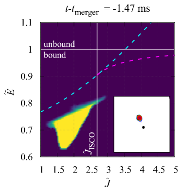
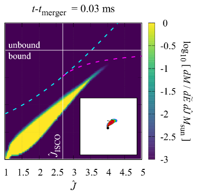
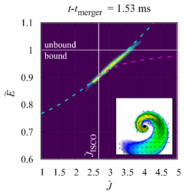
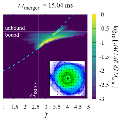
Figure 14: Distribution of material on the phase space of specific energy $\tilde{E}$ and specific angular momentum normalized by the mass of the remnant black hole $\hat{J}$ for a binary with $M_{\mathrm{BH}}=3\,M_{\odot}$, $\chi=0$, $M_{\mathrm{NS}}=1.35\,M_{\odot}$, and $R_{\mathrm{NS}}=$12.3\text{\,}\mathrm{km}$$ ($Q\approx 2.2$, $\mathcal{C}=0.162$) modeled by a piecewise polytrope called H (Read et al., 2009b). The left top panel shows the distribution in the final stage of the inspiral. The right top panel shows the distribution at the onset of merger. The distribution is broadened and spans a wide range of $\tilde{E}$ and $\hat{J}$ due to the angular momentum transport. The left bottom panel shows the state after the infall of the material with low $\hat{J}$. Only the material with the angular momentum exceeding that for the innermost stable circular orbit, $\hat{J}_{\mathrm{ISCO}}$, remains outside the black hole. This material has gained exclusively the energy during the coalescence of the black hole and the major part of the neutron star. The right bottom panel shows the stage in which the remnant disk establishes a quasisteady state. The purple dashed curves denote the relation for stable circular orbits (Bardeen et al., 1972), and the material along this curve is the remnant disk. The cyan dashed curves denote the relation for material with a fixed periastron distance, and the material along this curve consists of the dynamical ejecta and fallback material. Image reproduced with permission from Hayashi et al. (2021), copyright by APS.

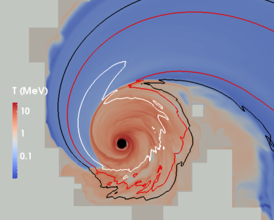
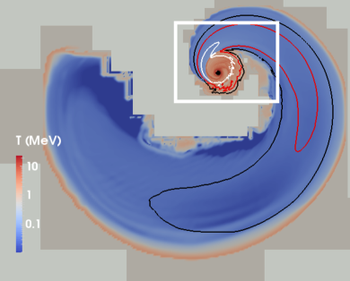
Figure 15: Temperature profile and the location of the apparent horizon (black filled circle) at $7\text{\,}\mathrm{ms}$ after the onset of merger for a binary with $M_{\mathrm{BH}}=7\,M_{\odot}$, $\chi=0.9$, $M_{\mathrm{NS}}=1.2\,M_{\odot}$, and $R_{\mathrm{NS}}=$13.5\text{\,}\mathrm{km}$$ ($Q\approx 5.8$, $\mathcal{C}=0.130$) modeled by the FSU2.1 equation of state (Todd-Rutel and Piekarewicz, 2005; Shen et al., 2011). The left panel is magnification of the white box in the right panel. The white, red, and black curves denote ${10}^{11}$, ${10}^{10}$, and ${10}^{9}\text{\,}\mathrm{g}\text{\,}{\mathrm{cm}}^{-3}$, respectively. Image reproduced with permission from Brege et al. (2018), copyright by APS.

The outermost part of the tidal tail obtains energy sufficient to become unbound from the remnant black hole. Figure 14 visualizes the process of dynamical mass ejection on the phase space of the specific energy and the specific angular momentum for a system with $M_{\mathrm{BH}}=3\,M_{\odot}$, $\chi=0$, $M_{\mathrm{NS}}=1.35\,M_{\odot}$, and $R_{\mathrm{NS}}=$12.3\text{\,}\mathrm{km}$$ ($Q\approx 2.2$, $\mathcal{C}=0.162$) modeled by a piecewise polytrope called H (Hayashi et al., 2021). Here, unboundedness is identified by the criterion $-u_{t}>1$, which is suitable for dynamical mass ejection as far as the spacetime is approximated as stationary, because the shock heating, and hence, the contribution of the internal energy, does not play a role. If the internal energy contributes significantly, a reasonable criterion may be defined based on $-hu_{t}$ taking the offset associated with the composition into account (see, e.g., Fujibayashi et al., 2020a). First, the outer part acquires the angular momentum and also the energy via the tidal torque (from the left top to the right top panels). Next, it gains exclusively the energy via work done by impulsive outward radial force, which is likely to be associated with the infall of the major part of the neutron star to the black hole (from the right top to the left bottom panels). If the energy of a fluid element exceeds the gravitational binding energy, the element escapes from the system as the dynamical ejecta.

Material behind the dynamical ejecta also acquires some energy but remains bound to the remnant black hole, and thus it eventually falls back onto the disk. The disk and fallback components may approximately be distinguished by temperature higher and lower than $0.1$–$1\text{\,}\mathrm{MeV}$, respectively, as shown in Fig. 15 generated by Brege et al. (2018), because the shock interaction sets in when the fallback material hits the outer edge of the disk. Although the longterm fallback dynamics cannot be fully tracked in current simulations of black hole–neutron star binary coalescences, estimated fallback rates of the mass are found to coincide with the well-known $t^{-5/3}$ law for tidal disruption events (Chawla et al., 2010; Kyutoku et al., 2015; Brege et al., 2018, see also Rosswog 2007 for early Newtonian work).

The left bottom panel of Fig. 14 implies that the fallback material and the dynamical ejecta may be considered to be launched from an approximately common periastron. Taking the $t^{-5/3}$ fallback behavior into account, the process depicted here might seem similar to tidal disruption of stars by supermassive black holes in slightly unbound, hyperbolic encounters (Rees, 1988; Phinney, 1989). However, it should be remarked that gravitational-wave-driven mergers of compact object binaries occur in a strongly bound, quasicircular orbit. Therefore, it is not trivial a priori that even a finite amount of material could be ejected by tidal disruption in black hole–neutron star binary coalescences.

The process of tidal disruption described in Fig. 13 is qualitatively common for systems with a large neutron-star radius, a small black-hole mass, and/or a high black-hole spin. However, quantitative details depend on the parameters of the binary. The orientation of the black-hole spin also introduces qualitative differences in the merger dynamics and morphology of the remnant. In the following, we review the dependence on these parameters.

3.3.1 Dependence on the equation of state

As found from the analysis of Sect. 1.3 and Sect. 2, the merger process depends on the compactness of the neutron star, which is determined by the equation of state. Systematic studies performed employing a variety of piecewise polytropes clearly show that neutron stars with smaller compactnesses are tidally disrupted more easily (Kyutoku et al., 2010, 2011a, 2015). This tendency also holds for nuclear-theory-based tabulated equations of state (Kyutoku et al., 2018; Brege et al., 2018).

Even if the compactness and the mass are identical, the density profiles generally differ among neutron stars modeled by different equations of state. If the density profile is more centrally condensed, the neutron star is less subject to tidal disruption as discussed in Sect. 1.3.2. This tendency is demonstrated by a study employing two-piecewise polytropes with different adiabatic indices for the core region (Kyutoku et al., 2010). Specifically, if the adiabatic index for the core region is smaller, the neutron star with a given compactness is more centrally condensed and less subject to tidal disruption.

3.3.2 Dependence on the mass ratio

As indicated by the analysis of Sect. 1.3 and Sect. 2, the possibility of tidal disruption increases as the mass ratio decreases. For example, the amount of the mass remaining outside the black hole is likely to be larger for the lower mass ratio. This dependence is particularly important for nonspinning black holes, because significant tidal disruption occurs only for low-mass black holes such as those in the putative mass gap (Shibata et al., 2009, 2012). Stated differently, for a plausibly realistic mass ratio of $Q\gtrsim 4$, the neutron star can be tidally disrupted only if the black hole has a high prograde spin, as we discuss in Sect. 3.3.3.

After the discovery of binary neutron stars by gravitational waves, very-low-mass black hole–neutron star coalescences acquire renewed interest (Foucart et al., 2019a, b; Hayashi et al., 2021; Most et al., 2021a, see Sect. 1.4.4 for definition of “very low mass”). The primary reason for this is that they could be potential mimickers of binary-neutron-star coalescences, rendering astrophysical interpretation of gravitational-wave sources ambiguous (Hinderer et al., 2019; Kyutoku et al., 2020). Distinguishing very-low-mass black hole–neutron star binaries and binary neutron stars would be invaluable for gaining knowledge about the maximum mass of neutron stars, the mass gap between black holes and neutron stars (see, e.g., Kreidberg et al., 2012), and the formation mechanism of these compact objects, i.e., stellar core collapse and supernova explosions.

Recent numerical simulations have shown that susceptibility to tidal disruption is not reflected monotonically in the remnant material for very-low-mass-ratio systems (Foucart et al., 2019b; Hayashi et al., 2021; Most et al., 2021a). Rather, the mass of the remnant disk saturates to a value of $\sim\order{0.1}\,M_{\odot}$ for the case in which the black hole is nonspinning (see also Brege et al. 2018 and Appendix of Hayashi et al. 2021). Quantitatively, the saturated value of the disk mass depends on the equation of state. Moreover, the mass of the dynamical ejecta, which increases with decreasing $Q$ down to a moderately large values of $Q=Q_{\mathrm{peak}}\sim 3$, begins to decrease as the mass ratio decreases for $Q<Q_{\mathrm{peak}}$ (Hayashi et al., 2021). The precise value of $Q_{\mathrm{peak}}$ again depends on the equation of state. We will discuss quantitative dependence of the remnant disk and the dynamical ejecta on the mass ratio later in this section.

We note that, while the physical reason of the behavior at very low-mass ratios described above is not fully understood yet, it may not be unexpected taking the fact that an extremely low-mass black hole with $M_{\mathrm{BH}}\ll M_{\mathrm{NS}}(Q\ll 1)$ cannot make the neutron star unbound because of the tiny contribution of such a minute black hole to the dynamics of the entire system. Related simulations have been performed in the context of consumption of a neutron star by an endoparasitic black hole at the center (East and Lehner, 2019; Richards et al., 2021).

3.3.3 Dependence on the black-hole spin (I) aligned spin

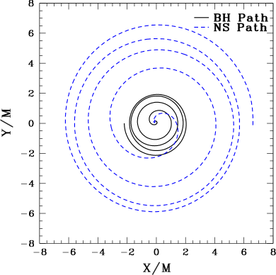
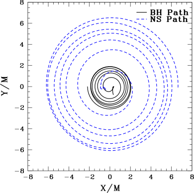
Figure 16: Coordinate trajectory of the black hole (black solid curve) and the neutron star (blue dashed curve) on the orbital plane for binaries with $Q=3$, $\mathcal{C}=0.145$ modeled by a $\Gamma=2$ polytrope, and $\chi=0$ (left) and $\chi=0.75$ (right). Image reproduced with permission from Etienne et al. (2009), copyright by APS.

The spin of the black hole quantitatively modifies the orbital evolution in the late inspiral phase and the merger dynamics. First, we focus on the cases in which the black-hole spin is (anti-)aligned with respect to the orbital angular momentum of the binary. Figure 16 generated by Etienne et al. (2009) shows the trajectories of the black hole and the neutron star for systems characterized by $Q=3$, $\mathcal{C}=0.145$ modeled by a $\Gamma=2$ polytrope, and two different values of the spin parameter $\chi=0$ (left) and $\chi=0.75$ (right). Because a polytropic equation of state is adopted, the mass of the binary components can be scaled arbitrarily as discussed in Sect. 2.3. Both systems have the same values of initial orbital angular velocity normalized by the total mass, $Gm_{0}\Omega/c^{3}\approx 0.033$. The nonspinning ($\chi=0$) and spinning ($\chi=0.75$) systems merge after $\sim 4$ and $6$ orbits, respectively. The difference in the number of orbits is ascribed mainly to the spin-orbit interaction. Specifically, this interaction serves as repulsive force for a prograde spin of the black hole, $\chi>0$, and vice versa (see, e.g., Kidder et al. 1993; Kidder 1995 for two-body equations of motion in the post-Newtonian approximation). The repulsion for $\chi>0$ counteracts the gravitational pull between the binary components and reduces the orbital angular velocity to maintain a circular orbit for a given orbital separation (or a given circumferential radius of the orbit). Because the gravitational-wave luminosity is as sensitive to the orbital angular velocity as $\propto\Omega^{10/3}$, the approaching velocity associated with the radiation reaction is also decreased. This effect increases the lifetime of the binary. In addition, the spin-orbit repulsion decreases the radius of the innermost stable orbit and strengthens gravitational binding there (Bardeen et al., 1972). This further helps to increase the lifetime of a progradely-spinning black hole–neutron star binary, because it needs to emit a larger amount of energy to reach the innermost stable circular orbit than that for a nonspinning black hole. These effects increase the number of inspiral orbits.

The higher the prograde spin of the black hole, the neutron star is disrupted more easily, and thus, the disk formation and the mass ejection are more pronounced. This is clearly shown by comparing Figs. 12 and 13, between which the only difference is the spin of the black hole. Quantitatively, while the mass of the disk for $\chi=0$ is less than $${10}^{-3}$\,M_{\odot}$, it increases to $0.19\,M_{\odot}$ for $\chi=0.75$ in these examples. The mass of the dynamical ejecta also increases as the black-hole spin increases, specifically from $\ll${10}^{-3}$\,M_{\odot}$ to $0.01\,M_{\odot}$ in these examples (Kyutoku et al., 2015). These increases are ascribed primarily to the small radius of the innermost stable circular orbit with the prograde spin (Bardeen et al., 1972). As an extreme, it has been shown that about more than a half of the neutron-star material remains outside the remnant black hole right after the onset of merger for a binary with $Q=3$, $\mathcal{C}=0.144$ modeled by a $\Gamma=2$ polytrope, and $\chi=0.97$, which is the largest value of the spin parameter simulated for black hole–neutron star binaries to date (Lovelace et al., 2013). In light of the astrophysically plausible range of $Q$ and $\mathcal{C}$ (e.g., $Q\gtrsim 4$ and $\mathcal{C}\gtrsim 0.16$), it is remarkable that the prograde spin enables tidal disruption to occur for a binary which results in the plunge if the black hole is nonspinning. By contrast, if the spin of the black hole is retrograde, the neutron star is swallowed by the black hole without tidal disruption even if $Q<3$ for a wide range of equations of state. We defer further quantitative discussions to Sect. 3.4.2.

If tidal disruption occurs in a binary with a spinning black hole and a realistic mass ratio of $Q\gtrsim 4$, the elongated neutron star can be swallowed by the black hole through a narrow region of its large surface (Kyutoku et al., 2011a). This feature is advantageous for exciting nonaxisymmetric, fundamental quasinormal modes of the remnant black hole as we discuss in Sect. 3.6. This does not occur for nonspinning black holes, because the tidal disruption is possible only for a binary with a low mass ratio of $Q\lesssim(3\mathcal{C})^{-3/2}$ [cf., Eq. (9) and Fig. 10] and thus for a black hole with a small surface. For such a case, the tidally-disrupted material is swallowed through a wide region of the black-hole surface, and the quasinormal-mode excitation is suppressed. These differences are reflected in both gravitational waveforms and spectra as predicted by a black-hole perturbation study (Saijo and Nakamura, 2000, 2001).

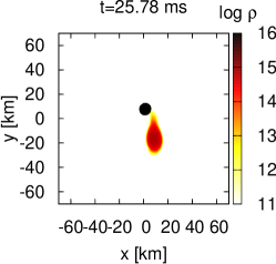
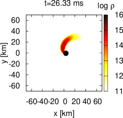
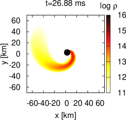
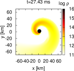
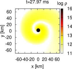
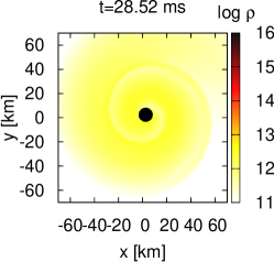
Figure 17: Same as Fig. 12 but for a binary with $M_{\mathrm{BH}}=4.05\,M_{\odot}$, $\chi=0.5$, $M_{\mathrm{NS}}=1.35\,M_{\odot}$, and $R_{\mathrm{NS}}=$11.6\text{\,}\mathrm{km}$$ ($Q=3$, $\mathcal{C}=0.172$) modeled by a piecewise polytrope called HB (Read et al., 2009b). Image reproduced with permission from Kyutoku et al. (2011a), copyright by APS.

Figure 17 illustrates the case described above, i.e., the tidally-elongated neutron star is swallowed through a narrow region of the black-hole surface (Kyutoku et al., 2011a). This system is characterized by $M_{\mathrm{BH}}=4.05\,M_{\odot}$, $M_{\mathrm{NS}}=1.35\,M_{\odot}$, $R_{\mathrm{NS}}=$11.6\text{\,}\mathrm{km}$$ ($Q=3$, $\mathcal{C}=0.172$) modeled by a piecewise polytrope called HB, and a moderately high and prograde spin of $\chi=0.5$. Tidal disruption occurs at an orbit outside but close to the innermost stable circular orbit. The dense part of disrupted material does not have a sufficient time for winding around the black hole before the infall. Thus, it falls into the black hole in a significantly nonaxisymmetric manner and excites quasinormal-mode oscillations. This behavior is frequently found for a binary with a high mass ratio and a high black-hole spin. Conversely, for a retrograde spin, tidal disruption becomes insignificant even for a small value of $Q=2$–$3$ (Kyutoku et al., 2011a). An alternative interpretation of this finding is that the orientation of the black-hole spin plays an important role. We will discuss this viewpoint for a general inclination angle in Sect. 3.3.4.

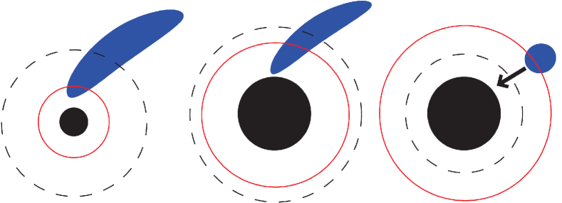
Figure 18: Schematic picture for three types of merger processes. The filled circle, the solid red circle, and the black dashed circle denote the black hole, the innermost stable circular orbit, and the radius at which tidal disruption occurs, respectively. The deformed ellipsoid denotes the neutron star. The left, middle, and right panels correspond to the types 1, 2, and 3, described in the body text, respectively. Image adapted from Kyutoku et al. (2011a), copyright by APS.

To summarize, numerical-relativity simulations have revealed that the merger process may be classified into three types according to the mass and the spin of black holes for a given equation of state (see also Pannarale et al. 2013, 2015a for relevant classifications):

1. The neutron star is tidally disrupted at an orbit far from the innermost stable circular orbit. This occurs for the cases in which the black-hole mass is small and/or the black-hole spin is prograde and sufficiently high.

2. The neutron star is tidally disrupted at an orbit close to the innermost stable circular orbit. This occurs for the cases in which the black-hole mass is not small and the black-hole spin is prograde and high.

3. The neutron star is not tidally disrupted. This occurs for the cases in which the black-hole mass is not small and/or the black-hole spin is retrograde or prograde but not high. An approximate criterion for tidal disruption is found in Eq. (9).

These three types are displayed schematically in Fig. 18. The differences of merger processes for these types, particularly that between 1 and 2, are imprinted in gravitational waveforms and spectra described in Sect. 3.6.

3.3.4 Dependence on the black-hole spin (II) inclined spin

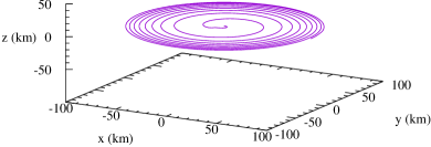
Figure 19: Evolution of the coordinate separation between the black hole and the neutron star for binaries with $M_{\mathrm{BH}}=4.05\,M_{\odot}$, $M_{\mathrm{NS}}=1.35\,M_{\odot}$, and $R_{\mathrm{NS}}=$11.1\text{\,}\mathrm{km}$$ ($Q=3$, $\mathcal{C}=0.180$) modeled by a piecewise-polytropic approximation of the APR4 equation of state (Akmal et al., 1998). The spin of the black hole is zero for the left panel and $\chi=0.75$ with the inclination angle $\iota\approx$$$ for the right panel. The $z$-axis is taken to be the direction of the total angular momentum at the initial instant. This figure is generated from data of Kyutoku et al. (2021).

The inclination angle has a qualitative impact on the inspiral and merger dynamics (Foucart et al., 2011, 2013b; Kawaguchi et al., 2015; Foucart et al., 2017, 2021). Figure 19 compares typical orbital evolution of black hole–neutron star binaries for which the spin of the black hole is absent or (anti-)aligned with respect to the orbital angular momentum of the binary (left: $\chi=0$) and inclined (right: $\chi=0.75$ and $\iota\approx$$$). The reflection symmetry about the orbital plane is lost in the presence of spin misalignment. Because the orbital angular velocity vector is inclined with respect to the total angular momentum of the system, the vector normal to the orbital plane precesses approximately around the total angular momentum during the inspiral phase (Apostolatos et al., 1994; Kidder, 1995; Racine, 2008).

The spin misalignment also reduces the degree of tidal disruption, as well as the masses of the remnant disk and the dynamical ejecta, for the same magnitude of the spin. This is because the spin-orbit coupling is proportional to, in the post-Newtonian terminology, the inner product $\mathbf{S}\dotproduct\mathbf{L}$ of the spin angular momentum $\mathbf{S}$ and the orbital angular momentum $\mathbf{L}$. The effect of the black-hole spin on the radius of the innermost stable circular orbit, or an innermost stable spherical orbit (Hughes, 2001; Buonanno et al., 2006; Fragile et al., 2007; Stone et al., 2013), is also determined primarily by this inner product. Thus, the spin-orbit repulsion for a given magnitude of the spin becomes weak as the inclination angle increases. For systems with the black-hole spin being confined in the orbital plane, $\mathbf{S}\dotproduct\mathbf{L}\approx 0$, the spin of the black hole is likely to play only a minor role in tidal disruption of the neutron star irrespective of its magnitude, while systematic surveys have not yet been performed.

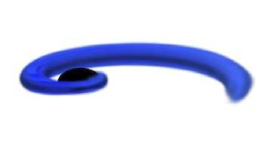
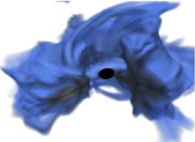
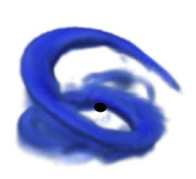
Figure 20: Three-dimensional plot of the rest-mass density and the location of the apparent horizon (denoted by the filled black region) for binaries with $Q=7$, $\chi=0.9$, and $\mathcal{C}=0.144$ ($R_{\mathrm{NS}}=$14.4\text{\,}\mathrm{km}$$ if we suppose a $1.4\,M_{\odot}$ neutron star) modeled by a $\Gamma=2$ polytrope. The angles between the spin angular momentum of the black hole and the orbital angular momentum of the binary are $0\mathrm{°}$ and $40\mathrm{°}$ for the left and right panels, respectively. The top and bottom panels show snapshots at different times. Image reproduced with permission from Foucart et al. (2013b), copyright by APS.

Orbital precession caused by the spin misalignment introduces qualitative differences also in the morphology of the disrupted material (Foucart et al., 2013b; Kawaguchi et al., 2015). Because the misalignment breaks the reflection symmetry, the remnant also exhibits a reflection-asymmetric structure. Figure 20 generated by Foucart et al. (2013b) shows three-dimensional plots of the rest-mass density and the region inside the apparent horizon. The system on the left column is characterized by $Q=7$, $\mathcal{C}=0.144$ modeled by a $\Gamma=2$ polytrope, and $\chi=0.9$ aligned with the orbital angular momentum of the binary. The merger dynamics and the morphology of the remnant are essentially the same as those described in Fig. 13. The system on the right column of Fig. 20 has the same parameters as those on the left column, except that the black-hole spin has an inclination angle of $\iota=$$$ with respect to the orbital angular momentum. The tidal tail of this system inherits precessing motion of the inspiral phase. Accordingly, it does not form a circularized disk immediately after single orbital revolution. Instead, the tidal tail eventually collides with itself from various directions and forms a thick torus. The inclination angle between the angular momentum of the remnant torus and the spin angular momentum of the remnant black hole becomes smaller than the inclination angle during the inspiral phase, $\iota$, because a substantial fraction of the orbital angular momentum is brought into the black hole by the infalling neutron-star material (Foucart et al., 2011; Kawaguchi et al., 2015). This effect is more significant for lower mass-ratio systems, for which the initial spin angular momentum of the black hole accounts for a smaller fraction of the total angular momentum.

In the long run, a tilted disk will evolve in a manner different from an aligned one via the Lense-Thirring precession (Bardeen and Petterson, 1975; Papaloizou and Pringle, 1983), magnetically-induced turbulent viscosity (Fragile et al., 2007) and/or magnetic coupling with the remnant black hole (McKinney et al., 2013). Longterm evolution of a remnant torus of precessing black hole–neutron star binaries with realistic microphysics is a subject for future studies in numerical relativity (but see Mewes et al. 2016 for pure hydrodynamics).

3.4 Remnant

In this Sect. 3.4, we present quantitative details of the remnant black hole, disk, fallback material, and dynamical ejecta derived by merger simulations. Unless explicitly stated, we discuss the cases in which the spin of the black hole is aligned with respect to the orbital angular momentum and the system possesses reflection symmetry about the orbital plane. We will make it explicit when we consider the effects of the spin misalignment. The longterm evolution of the remnant disk and associated outflows are discussed separately in Sect. 3.5.

3.4.1 Black hole

The mass and the spin of the black hole change during merger, because it swallows the material of the neutron star. The mass of the remnant black hole $M_{\mathrm{BH,f}}$ is approximately estimated by (Shibata and Uryū, 2007)

$$M_{\mathrm{BH,f}}\approx M_{\mathrm{BH}}+M_{\mathrm{NS}}-M_{r>{r_{\mathrm{AH}}}}-E_{\mathrm{GW}},$$ (39)

where $M_{r>{r_{\mathrm{AH}}}}$ denotes the mass of the material remaining outside the black hole, which is composed of the remnant disk, the fallback material, and the dynamical ejecta, and $E_{\mathrm{GW}}$ denotes the energy carried away by gravitational radiation (see Duez et al. 2008; Shibata et al. 2009 for other methods of estimation). Because a large fraction of the neutron-star material falls into the black hole for most cases and also $E_{\mathrm{GW}}$ is much smaller than the total rest-mass energy of the system, $M_{\mathrm{BH,f}}$ is larger than $0.9m_{0}$ except for nearly-extremal spins (Lovelace et al., 2013). Because both $M_{r>{r_{\mathrm{AH}}}}$ and $E_{\mathrm{GW}}$ decrease as the spin of the black hole decreases, $M_{\mathrm{BH,f}}$ becomes close to $m_{0}$ for small values of $\chi$ and/or large inclination angles. Specifically, the difference between $M_{\mathrm{BH,f}}$ and $m_{0}$ is only a few percent for anti-aligned, retrograde spins of $\chi=-0.5$ (stated differently, $\chi=0.5$ and $\iota=$$$; Kyutoku et al., 2011a).

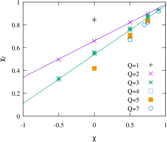
Figure 21: Spin parameter of the remnant black hole, $\chi_{\mathrm{f}}$, for a range of binary parameters as a function of the initial spin parameter, $\chi$. The solid lines denote the fitting for the results of $Q=2$ and $3$ (Kyutoku et al., 2011a). This figure is generated from data of Etienne et al. (2009); Kyutoku et al. (2010); Foucart et al. (2011); Kyutoku et al. (2011a); Foucart et al. (2012); Kyutoku et al. (2015). If the neutron-star mass and/or equation of state are varied in a single paper, the results are averaged.

The spin parameter of the remnant black hole $\chi_{\mathrm{f}}$ is determined primarily by the mass ratio of the binary, $Q$, and the initial spin parameter of the black hole, $\chi$ (Kyutoku et al., 2011a). Figure 21 shows the spin parameter of the remnant black hole as a function of the initial spin parameter $\chi$ for various mass ratios obtained by pure hydrodynamics simulations performed by several groups with various numerical implementations. Some particular combinations of $Q$ and $\chi$ are simulated by several groups independently, and results are overplotted. Taking inherent variation associated with the neutron-star mass, the neutron-star equation of state, and the methods for evaluating $\chi_{\mathrm{f}}$ (Duez et al., 2008; Shibata et al., 2009) into account, all the results are consistent among independent groups. This figure shows that the dependence on the initial spin parameter is more pronounced for higher mass ratios. The reason for this is that, as we describe below, the spin angular momentum becomes dominant and the orbital angular momentum gives a minor contribution in such systems. Meanwhile, the remnant spin parameter is found to depend only weakly on the equation of state (not shown in this figure), and this fact indicates that the material remaining outside the remnant black hole takes only a minor fraction of the mass and the angular momentum for the systems considered. It is also found that the remnant spin parameter is larger than that for binary black holes with the same values of $Q$ and $\chi$ for the case in which tidal disruption occurs. For example, the coalescence of equal-mass, nonspinning binary black holes is known to form a Kerr black hole with $\chi_{\mathrm{f}}\approx 0.686$ (Scheel et al., 2009), which is significantly smaller than $\chi_{\mathrm{f}}\approx 0.84$ for black hole–neutron star binaries (Etienne et al., 2009; Foucart et al., 2019b). This difference stems from the fact that black hole–neutron star binaries which result in tidal disruption do not experience orbits as close as those in binary black holes. Accordingly, black hole–neutron star binaries do not emit gravitational waves as strongly as binary black holes do.

Qualitative dependence of $\chi_{\mathrm{f}}$ on $Q$ and $\chi$ can be understood by the following analysis. The total angular momentum of two point particles in a circular orbit with the orbital angular velocity $\Omega$ is given in Newtonian gravity by

$$J_{\mathrm{orb}}=\frac{G^{2/3}M_{\mathrm{BH}}M_{\mathrm{NS}}}{(\Omega m_{0})^{1/3}}.$$ (40)

The spin parameter of the system, which is also denoted by $\chi_{\mathrm{f}}$ here, may be given approximately by

$$\chi_{\mathrm{f}} =\frac{cJ_{\mathrm{orb}}/G+\chi M_{\mathrm{BH}}^{2}}{m_{0}^{2}}$$

$$=\frac{\pqty{Gm_{0}\Omega/c^{3}}^{-1/3}Q+\chi Q^{2}}{(Q+1)^{2}},$$ (41)

where we assumed that the spin of the black hole is aligned with the orbital angular momentum. Because the orbital angular velocity at the onset of merger or at tidal disruption is given by $Gm_{0}\Omega/c^{3}\sim 0.05$–$0.1$ for a wide range of binary parameters, $(Gm_{0}\Omega/c^{3})^{-1/3}$ takes a narrow range of $2.2$–$2.7$. Thus, as far as we may neglect the mass and the angular momentum of the remnant material and the energy carried away by gravitational radiation, $\chi_{\mathrm{f}}$ gives the spin parameter of the remnant black hole. This expression depends primarily on the mass ratio and the initial spin parameter of the black hole, and furthermore, explains the pronounced dependence on the initial spin parameter for a high mass-ratio system.

Numerical simulations suggest that the remnant black hole is not overspun by the infall of the neutron star, respecting the cosmic censorship conjecture (Penrose, 1969, 2002). Rather, fitting formulae derived in Kyutoku et al. (2011a) predict that the spin parameter should decrease during merger for nearly-extremal spins as shown at the right edge of Fig. 21. Simulations of a system with $Q=3$ and $\chi=0.97$ illustrate that the spin parameter indeed decreases below $0.97$ (Lovelace et al., 2013), consistently with the prediction of the fitting formulae. Detailed phenomenological models of both the mass and the spin of the remnant black hole are provided by Pannarale (2013, 2014).

The magnitude of the spin parameter of the remnant black hole decreases as the inclination angle increases for a given value of the magnitude of the spin parameter of the initial black hole (Foucart et al., 2011; Kawaguchi et al., 2015; Foucart et al., 2017). This is because the magnitude of the spin angular momentum, which is a vectorial quantity, does not increase as sizably as the mass of the remnant black hole in the presence of the inclination. The magnitude of the spin parameter can even decrease from the initial value for a large inclination angle (Kawaguchi et al., 2015; Foucart et al., 2017) in the same manner as the cases with anti-aligned spins shown in Fig. 21. The direction of the spin of the remnant black hole is approximately aligned with the total angular momentum of the system right before merger, as most of the orbital angular momentum is swallowed by the black hole.

3.4.2 Accretion disk, or material remaining outside the black hole

We separate discussions about the remnant disk into two parts. Here in Sect. 3.4.2, we describe dependence of the disk mass, or the mass of the remnant (see below), on binary parameters. Thermodynamic variables such as the rest-mass density of the remnant disk will be discussed later in Sect. 3.4.3.

Regarding the disk mass, early systematic surveys have rather focused on the total mass of the material remaining outside the black hole, $M_{r>r_{\mathrm{AH}}}$, without distinguishing bound and unbound components. This quantity can be derived more accurately than the disk or bound mass, which suffers from a subtle task of determining the boundary between bound and unbound components. Furthermore, $M_{r>r_{\mathrm{AH}}}$ is found to show clearer correlations with the neutron-star compactness than the disk or bound mass is. Thus, we base our discussions on $M_{r>r_{\mathrm{AH}}}$.

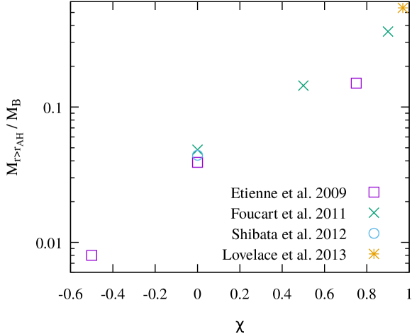
Figure 22: Summary of the mass of the material remaining outside the black hole, $M_{r>r_{\mathrm{AH}}}$, as a function of the spin parameter of the black hole for binaries with $Q=3$ and $\mathcal{C}\approx 0.145$ modeled by a $\Gamma=2$ polytrope computed by three independent groups. The vertical axis shows the fraction of $M_{r>r_{\mathrm{AH}}}$ to the baryon rest mass of the neutron star, $M_{\mathrm{B}}$. Note that these values are measured at different times in each simulation (see also Foucart, 2012). This figure is generated from data of Shibata et al. (2012); Etienne et al. (2009); Foucart et al. (2011); Lovelace et al. (2013).

To date, dependence of $M_{\mathrm{r>r_{\mathrm{AH}}}}$ on the spin parameter has been studied most extensively for a qualitative $\Gamma=2$ polytrope by several independent groups. Figure 22 plots the fractional baryonic mass of the material remaining outside the black hole obtained by three independent groups as a function of the spin parameter of the black hole for systems with $Q=3$ and $\mathcal{C}\approx 0.145$ modeled by the $\Gamma=2$ polytrope. Care must be taken for the fact that these quantities are measured at different times in each simulation, and particularly the result for $\chi=0.75$ is inferred as late as $\approx$25\text{\,}\mathrm{ms}$$ after the onset of merger for a hypothetical value of $M_{\mathrm{NS}}=1.35\,M_{\odot}$ (Etienne et al., 2009, Fig. 13). Taking this limitation into account, the results agree approximately for $\chi=0$ (Etienne et al., 2009; Foucart et al., 2011; Shibata et al., 2012). Figure 22 also shows that $M_{r>r_{\mathrm{AH}}}$ increases as the value of the spin parameter increases for $Q=3$ and this equation of state. Specifically, the values of $M_{r>r_{\mathrm{AH}}}/M_{\mathrm{B}}$ are approximately proportional to $\exp(b\chi)$ with $b\approx 2.5$–$3$ for a range displayed in Fig. 22. This enables us to reconfirm that the degree of tidal disruption depends strongly on the spin of the black hole.

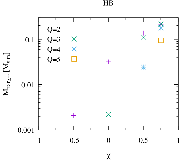
Figure 23: Mass of the material remaining outside the black hole at $10\text{\,}\mathrm{ms}$ after the onset of merger as a function of the spin parameter of the black hole for a variety of the mass ratio. The mass and the radius of the neutron star are fixed, respectively, to $M_{\mathrm{NS}}=1.35\,M_{\odot}$ and $R_{\mathrm{NS}}=$11.6\text{\,}\mathrm{km}$$ ($\mathcal{C}=0.172$) modeled by a piecewise polytrope called HB (Read et al., 2009b). This figure is generated from data of Kyutoku et al. (2011a).

Figure 23 plots $M_{r>r_{\mathrm{AH}}}$ as a function of the spin parameter of the black hole for systems with $M_{\mathrm{NS}}=1.35\,M_{\odot}$ and $R_{\mathrm{NS}}=$11.6\text{\,}\mathrm{km}$$ ($\mathcal{C}=0.172$) modeled by a piecewise polytrope called HB, which approximates soft nuclear-theory-based equations of state. This figure again illustrates the importance of the black-hole spin depicted in Fig. 22. Quantitatively, $M_{r>r_{\mathrm{AH}}}$ becomes as large as $\approx 0.1\,M_{\odot}$ for $\chi=0.75$ even if the compactness is realistically large with this soft equation of state and the mass ratio $Q$ is as high as $5$. Various subsequent studies have further shown that large values of the spin parameter allow such significant tidal disruption to occur even for $Q\approx 7$, which corresponds to typical masses of Galactic black holes, $\approx 10\,M_{\odot}$ (Foucart et al., 2013b, 2014; Kyutoku et al., 2015). Conversely, it is highly unlikely that the neutron star with $\mathcal{C}\gtrsim 0.17$ is disrupted by a black hole with $M_{\mathrm{BH}}\gtrsim 10\,M_{\odot}$ to leave material of $\gtrsim 0.1\,M_{\odot}$ unless the spin parameter is as high as $\chi\gtrsim 0.9$.

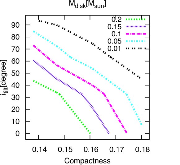
Figure 24: Contour for the mass of the bound material (denoted by $M_{\mathrm{disk}}$ in this figure) at $10\text{\,}\mathrm{ms}$ after the onset of merger on the compactness-inclination angle (denoted by $i_{\mathrm{tilt}}$ in this figure) plane for binaries with $M_{\mathrm{BH}}=6.75\,M_{\odot}$, $\chi=0.75$, and $M_{\mathrm{NS}}=1.35\,M_{\odot}$ ($Q=5$). The mass of the unbound material is excluded. Image reproduced with permission from Kawaguchi et al. (2015), copyright by APS.

As the inclination angle of the black-hole spin increases, the degree of tidal disruption and thus the mass of the remnant disk decrease (Foucart et al., 2011, 2013b; Kawaguchi et al., 2015). Figure 24 shows contours for the mass of the bound material only (not $M_{r>r_{\mathrm{AH}}}$). The masses of the black hole and the neutron star are fixed to be $M_{\mathrm{BH}}=6.75\,M_{\odot}$ and $M_{\mathrm{NS}}=1.35\,M_{\odot}$, respectively, and the magnitude of the black-hole spin is fixed to be $\chi=0.75$. This figure shows that the mass of the bound material decreases as the inclination angle increases. A similar trend holds for the unbound material and thus for the total mass remaining outside the black hole. Quantitatively, the mass of the bound material decreases from $0.1\,M_{\odot}$ (magenta) to $0.01\,M_{\odot}$ (black) with the increase of the inclination angle by only $\approx$$$–$30\mathrm{°}$ for a given value of the compactness at $\mathcal{C}\lesssim 0.17$. It has been pointed out that the mass of the material remaining outside the black hole with inclined spins is approximately reproduced by a model with an aligned black-hole spin whose magnitude derives the same radius of the innermost stable (circular or spherical) orbits as that of the original configuration (Foucart et al., 2013b; Stone et al., 2013) or, more simply, by a model with an aligned spin whose dimensionless magnitude is $\chi\cos\iota$ (Kawaguchi et al., 2015). The effect of the spin orientation has not been explored systematically over the parameter space, and this is a subject for future study. Figure 24 also shows that the mass of the bound material decreases as the compactness of the neutron star increases. We discuss the dependence of $M_{r>r_{\mathrm{AH}}}$ on the neutron-star compactness below, going back to the aligned-spin systems.

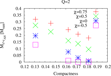
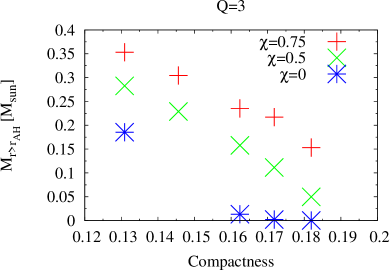
Figure 25: Mass of the material remaining outside the black hole at $10\text{\,}\mathrm{ms}$ after the onset of merger for binaries with $M_{\mathrm{NS}}=1.35\,M_{\odot}$ as a function of the compactness, which is varied by adopting a one-parameter family of piecewise polytropes. The spin parameter of the black hole is also varied. The left and right panels show the results of systems with $Q=2$ and $3$, respectively. Image adapted from Kyutoku et al. (2011a), copyright by APS.

Figure 25 plots $M_{r>r_{\mathrm{AH}}}$ as a function of the compactness for $Q=2$ (left) and $Q=3$ (right). The mass of the neutron star is fixed to be $M_{\mathrm{NS}}=1.35\,M_{\odot}$, and the compactness is varied by adopting a one-parameter family of piecewise polytropes (see Kyutoku et al. 2011a for the details). The values of the spin parameter are also varied systematically. This figure shows that $M_{r>r_{\mathrm{AH}}}$ decreases approximately linearly as the compactness increases until the value decreases to $\lesssim 0.01\,M_{\odot}$. This trend holds irrespective of the values of $Q$ or $\chi$. Figure 25 also shows that $M_{r>r_{\mathrm{AH}}}$ increases steeply as the spin parameter of the black hole increases as already seen in Figs. 22 and 23. Quantitatively, $M_{r>r_{\mathrm{AH}}}\gtrsim 0.1\,M_{\odot}$ is achieved for a wide range of compactness, $\mathcal{C}\lesssim 0.18$, if the black-hole spin is as high as $0.5$ for $Q=2$ and $0.75$ for $Q=3$.

Although the primary effect of the equation of state is captured by the compactness of the neutron star, the density profile also affects the susceptibility to tidal disruption. A comparison performed using a two-parameter family of piecewise polytropes shows that the mass of the material remaining outside the black hole decreases by more than a factor of $2$ for a centrally-condensed profile of the neutron star even if the compactness is approximately the same (Kyutoku et al., 2010, 2011b). This is because the central condensation tends to suppress the degree of tidal deformation and thus tidal disruption is appreciably delayed from the onset of mass shedding. We note that it has been pointed out that the correlation of $M_{r>r_{\mathrm{AH}}}$ with the tidal deformability, $\Lambda$, is not stronger than that with the compactness (Foucart, 2012; Foucart et al., 2018). Thus, neither the compactness nor the tidal deformability is fully appropriate to determine the amount of material remaining outside the black hole.

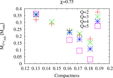
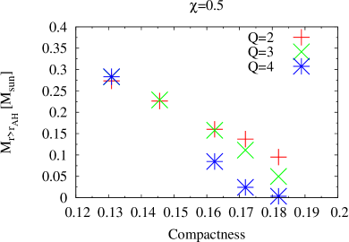
Figure 26: Same as Fig. 25 but for $\chi=0.75$ (left) and $\chi=0.5$ (right). The mass ratio is varied in each plot. Image adapted from Kyutoku et al. (2011a), copyright by APS.

Figure 26 shows the dependence of $M_{r>r_{\mathrm{AH}}}$ on the neutron-star compactness from another perspective for fixed values of $\chi=0.75$ (left) and $\chi=0.5$ (right). The mass of the neutron star is fixed to be $M_{\mathrm{NS}}=1.35\,M_{\odot}$. Again, it is found that $M_{r>r_{\mathrm{AH}}}$ increases approximately linearly as the compactness decreases irrespective of $Q$ or $\chi$. One notable feature that becomes clearly visible in this plot, although presaged in previous figures, is that the dependence of $M_{r>r_{\mathrm{AH}}}$ on the mass ratio, $Q$, becomes weak or even inverted from naive expectations at the small compactness of $\mathcal{C}\lesssim 0.15$. Analytic estimation in Sect. 1.3 suggests that the degree of tidal disruption and thus $M_{r>r_{\mathrm{AH}}}$ is likely to decrease as the black hole becomes massive, i.e., as $Q$ becomes high. This indeed holds for systems with a large neutron-star compactness, $\mathcal{C}\gtrsim 0.15$, but does not for $\mathcal{C}\lesssim 0.15$. This fact suggests that the dependence on the mass ratio is worth investigating in detail.

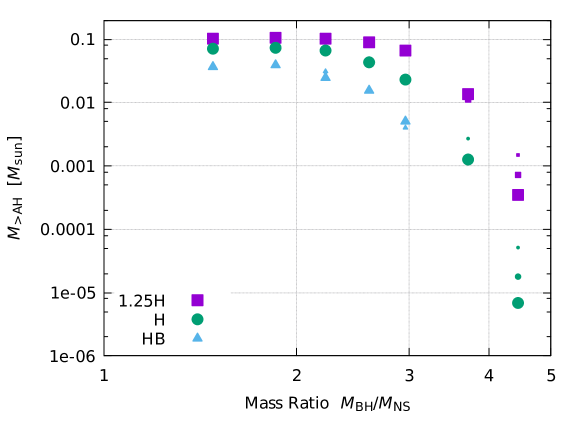
Figure 27: Mass of the material remaining outside the black hole at $12\text{\,}\mathrm{ms}$ after the onset of merger as a function of the mass ratio for binaries with $\chi=0$ and $M_{\mathrm{NS}}=1.35\,M_{\odot}$. Equations of state are varied by adopting a one-parameter family of piecewise polytropes called HB, H, and 1.25H (Read et al., 2009b; Lackey et al., 2012). Symbols with different sizes show the result obtained with different grid resolutions and are not visible for $M_{r>r_{\mathrm{AH}}}\gtrsim 0.01\,M_{\odot}$ on the scale of this figure. Image reproduced with permission from Hayashi et al. (2021), copyright by APS.

The dependence of $M_{r>r_{\mathrm{AH}}}$ on the mass ratio, $Q$, has recently been found to become very weak for very-low-mass and nonspinning black holes (Hayashi et al., 2021). Figure 27 shows $M_{r>r_{\mathrm{AH}}}$ as a function of $Q$ for nonspinning black hole–neutron star binaries with various equations of state. The mass of the neutron star is fixed to be $M_{\mathrm{NS}}=1.35\,M_{\odot}$. It is clearly shown that the value of $M_{r>r_{\mathrm{AH}}}$ levels off at $0.05$–$0.1\,M_{\odot}$ for $Q\lesssim 2$–$3$, where their precise values depend on the equation of state (and presumably the black-hole spin). We note that, as we discuss later in Sect. 3.4.5, $M_{r>r_{\mathrm{AH}}}$ is approximately identical to the mass of the remnant disk at this low-$Q$ saturation regime. In fact, such disappearance of the dependence on binary parameters may be observed in various regions of the parameter space for which the degree of tidal disruption increases (Brege et al., 2018; Hayashi et al., 2021) as is also suggested by Fig. 26. By what and how the saturation values of $M_{r>r_{\mathrm{AH}}}$ are determined have not been understood yet and may be counted as one of the unsolved problems about black hole–neutron star binaries.

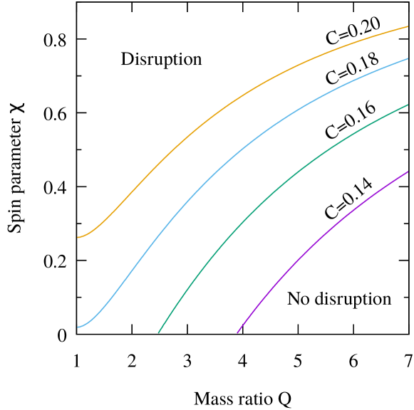
Figure 28: Criterion for tidal disruption predicted by the fitting formula of Foucart et al. (2018) for various compactnesses of neutron stars denoted by $C$. Here, the criterion is defined by the condition that more than 1% of the baryon rest mass of the neutron star is left outside the apparent horizon at $10\text{\,}\mathrm{ms}$ after the onset of merger. The baryon rest mass increases toward the left top region of this $Q$-$\chi$ plane for a given value of the compactness.

Fitting formulae for the mass of the material remaining outside the black hole are provided by Foucart (2012); Foucart et al. (2018). These fitting formulae are especially useful for deriving an approximate criterion for tidal disruption. Figure 28 displays the contour above which more than $1\%$ of the baryon rest mass of the neutron star is left outside the apparent horizon at $10\text{\,}\mathrm{ms}$ after the onset of merger for a given value of the neutron-star compactness (denoted by $C$ in this figure) on the $Q$-$\chi$ plane adopting a formula of Foucart et al. (2018). This formula is claimed to be accurate within $\sim 15\%$ for $1\leq Q\leq 7$ and $-0.5\leq\chi\leq 0.9$ for the case in which less than 30% of the baryon rest mass remains outside the apparent horizon. Because the equation of state is uncertain and the mass of the neutron star is different among realistic binaries, we draw contours for various values of the compactness, $\mathcal{C}$, which is the only finite-size effect of the neutron star taken into account in the formula adopted here (see Foucart et al. 2018 for another formula based on tidal deformability). This figure clearly shows that high prograde spins enable tidal disruption to occur outside the innermost stable circular orbit of massive black holes for a wide range of the neutron-star compactness. It should be cautioned that, however, all the previous simulations of black hole–neutron star binaries have not systematically varied masses of the neutron stars except for a scale-free, qualitative $\Gamma=2$ polytrope. Thus, predictions for $M_{\mathrm{NS}}\lesssim 1.2\,M_{\odot}$ or $M_{\mathrm{NS}}\gtrsim 1.5\,M_{\odot}$ need to be taken with particular care.

3.4.3 Thermodynamic properties of the disk

Continuing the discussions in Sect. 3.4.2, we summarize thermodynamic properties of the remnant disk. For a given value of the mass, the structure and time evolution of the remnant disk depend primarily on the total mass of the system, $m_{0}$. This is because the length scale of the system after merger is proportional to the mass of the remnant black hole, which agrees approximately with the total mass as we discussed in Sect. 3.4.1. If we focus on systems with a fixed value of $M_{\mathrm{NS}}$, the total mass of the system is controlled by the mass ratio as $m_{0}=(1+Q)M_{\mathrm{NS}}$.

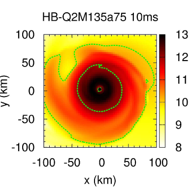
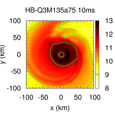
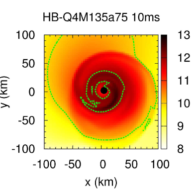
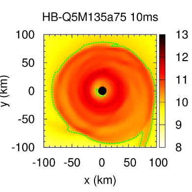
Figure 29: Profile of the rest-mass density and the location of the apparent horizon on the equatorial plane at $10\text{\,}\mathrm{ms}$ after the onset of merger for binaries with $\chi=0.75$, $M_{\mathrm{NS}}=1.35\,M_{\odot}$, and $R_{\mathrm{NS}}=$11.6\text{\,}\mathrm{km}$$ ($\mathcal{C}=0.172$) modeled by a piecewise polytrope called HB (Read et al., 2009b). The mass of the black hole, $M_{\mathrm{BH}}$, is varied. The total mass of the system is $4.05\,M_{\odot}$ (left top, $Q=2$), $5.4\,M_{\odot}$ (right top, $Q=3$), $6.75\,M_{\odot}$ (left bottom, $Q=4$), and $8.1\,M_{\odot}$ (right bottom, $Q=5$). The color map shows $\log_{10}(\rho[$\mathrm{g}\text{\,}{\mathrm{cm}}^{-3}$])$. The dashed curves denote isodensity contours of ${10}^{10}$ and ${10}^{12}\text{\,}\mathrm{g}\text{\,}{\mathrm{cm}}^{-3}$. Image reproduced with permission from Kyutoku et al. (2011a), copyright by APS.

Figure 29 displays the profiles of the rest-mass density of the remnant disk on the equatorial plane for systems with $\chi=0.75$, $M_{\mathrm{NS}}=1.35\,M_{\odot}$, $R_{\mathrm{NS}}=$11.6\text{\,}\mathrm{km}$$ ($\mathcal{C}=0.172$) modeled by a piecewise polytrope called HB but with different values of $M_{\mathrm{BH}}$ (Kyutoku et al., 2011a). This figure shows that the rest-mass density in the inner region is systematically higher for a smaller value of the total mass. Quantitatively, the maximum rest-mass density is $\approx${10}^{13}\text{\,}\mathrm{g}\text{\,}{\mathrm{cm}}^{-3}$$ for $m_{0}=4.05\,M_{\odot}$ ($Q=2$) and $\approx${10}^{11}\text{\,}\mathrm{g}\text{\,}{\mathrm{cm}}^{-3}$$ for $m_{0}=8.1\,M_{\odot}$ ($Q=5$). This difference cannot be ascribed to the difference in the mass of the material, because $M_{r>r_{\mathrm{AH}}}$ varies only by a factor of $\approx 2$ among the systems presented in this figure. Instead, reflecting the fact that the typical length scale such as the radius of the innermost stable circular orbit is smaller for a smaller value of $m_{0}$, the remnant disk is spatially more concentrated and the rest-mass density is increased. Conversely, low-density regions with $\rho\lesssim${10}^{10}\text{\,}\mathrm{g}\text{\,}{\mathrm{cm}}^{-3}$$ extend to a more distant region for larger values of $m_{0}$. Thus, the density gradient becomes shallow as the total mass increases.

The angular momentum profile after circularization is slightly sub-Keplerian by $\sim\order{10\%}$ due to pressure support, particularly in the outer part (Foucart et al., 2013b; Lovelace et al., 2013; Foucart et al., 2014). In addition, the disk is not geometrically thick at its formation. These features are qualitatively different from those of a geometrically-thick torus with constant specific angular momentum, which is typically adopted in longterm simulations for black hole–accretion disk systems (Fernández and Metzger, 2013; Just et al., 2015; Siegel and Metzger, 2017, 2018; Fernández et al., 2019; Miller et al., 2019a; Fernández et al., 2020).

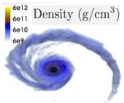
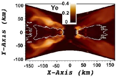
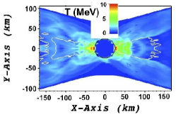
Figure 30: Three-dimensional plot of the rest-mass density (left), profile of the electron fraction on the meridional plane (middle), and that of the temperature in units of $\mathrm{MeV}$ (right) at $5\text{\,}\mathrm{ms}$ after the onset of merger for a binary with $M_{\mathrm{BH}}=7\,M_{\odot}$, $\chi=0.8$, $M_{\mathrm{NS}}=1.4\,M_{\odot}$, and $R_{\mathrm{NS}}=$12.7\text{\,}\mathrm{km}$$ ($Q=5$, $\mathcal{C}=0.163$) modeled by the LS220 equation of state (Lattimer and Swesty, 1991). Images repoduced with permission from Foucart et al. (2014), copyright by APS.

Although the profiles of the rest-mass density and the angular momentum are derived reasonably by pure hydrodynamics simulations, determining temperature and chemical composition of the disk requires implementations of a temperature- and composition-dependent equation of state and a scheme for neutrino transport. Such simulations are now becoming available along with gradual sophistication of the neutrino transport scheme (Deaton et al., 2013; Foucart et al., 2014, 2017; Kyutoku et al., 2018; Brege et al., 2018; Most et al., 2021a). Figure 30 generated by Foucart et al. (2014) illustrates a three-dimensional plot of the rest-mass density as well as the profiles of the electron fraction and the temperature on the meridional cross section at $5\text{\,}\mathrm{ms}$ after the onset of merger for a typical model. This simulation is performed with the LS220 equation of state (Lattimer and Swesty, 1991) and a leakage scheme for neutrino emission (but without neutrino absorption).

Maximum temperature in the accretion disk reaches $\gtrsim$10\text{\,}\mathrm{MeV}$$, i.e., $\gtrsim 1\%$ of the rest-mass energy of nucleons. For example, the system shown in Fig. 30 realizes $\sim$15\text{\,}\mathrm{MeV}$$ (Foucart et al., 2014). Other simulations by an independent group show that another set of systems with $M_{\mathrm{BH}}=5.4\,M_{\odot}$ and $M_{\mathrm{NS}}=1.35\,M_{\odot}$ ($Q=4$) also realizes $10$–$20\text{\,}\mathrm{MeV}$ (Kyutoku et al., 2018). These values are reasonably expected, because the temperature of the disk is increased by liberating the kinetic energy of the radial motion, whose velocity is $\sim\order{0.1c}$ at tidal disruption. Closer inspection reveals that the temperature is higher for a more compact neutron star, which is disrupted at a closer orbit to the black hole with higher velocity (Kyutoku et al., 2018). Although the maximum temperature exceeds $10\text{\,}\mathrm{MeV}$, the average temperature of the disk is typically $3$–$5\text{\,}\mathrm{MeV}$ at the disk formation, because the shock heating plays a major role only in a limited region of the disk.

The electron fraction of the remnant disk is $Y_{\mathrm{e}}\approx 0.1$ in most of the region, and it is increased to $0.2$–$0.3$ from the cold, $\beta$-equilibrium value of the neutron star for the region with high temperature of $\gtrsim$10\text{\,}\mathrm{MeV}$$ (Deaton et al., 2013; Foucart et al., 2014, 2017; Kyutoku et al., 2018). The reason for this increase is that the originally neutron-rich material of the remnant disk formed from the neutron star is protonized by capture reactions of thermally-produced electron/positron pairs onto nucleons. The profile of the electron fraction has been found to depend on binary parameters including equations of state (Foucart et al., 2014; Kyutoku et al., 2018). Systematic studies for the temperature and the chemical composition of the remnant disk have not been performed vigorously throughout the parameter space compared to studies in pure hydrodynamics for the mass and the rest-mass density. These may be one of the future directions.

In this Sect. 3.4.3, we have reviewed thermodynamic properties of the disk right after the onset of merger, e.g., at $\approx$10\text{\,}\mathrm{ms}$$ after the disk formation. Longterm evolution and states at late times are determined by ensuing neutrino cooling and magnetic-field amplification (see, e.g., Siegel and Metzger, 2017; Hossein Nouri et al., 2018; Fernández et al., 2019; Miller et al., 2019a; Christie et al., 2019). After the initial circularization stage, the disk temperature will gradually decrease due to the accretion and neutrino emission unless heating due to the effective viscosity associated with magnetohydrodynamical turbulence is highly efficient. As the disk expands and the rest-mass density decreases, the electron fraction will gradually increase due to weak interactions such as electron/positron captures and neutrino irradiation (Fujibayashi et al., 2020a, b; Just et al., 2021). In fact, these longterm evolution processes are partially observed in the simulations introduced above. However, these simulations are not realistic for $\gtrsim$10\text{\,}\mathrm{ms}$$ due to the lack of the angular momentum transport expected to be driven by magnetohydrodynamical effects. These topics will be discussed in Sect. 3.5.

3.4.4 Fallback material

When a part of the material outside the black hole becomes unbound as we discuss in Sect. 3.4.5, some material behind them simultaneously obtains energy but remains bound to the remnant black hole. The latter material travels to a distant region, turns around, joins the remnant disk with shock heating, and may energize electromagnetic transients such as extended and plateau emission of short-hard gamma-ray bursts (Rossi and Begelman, 2009; Lee et al., 2009; Metzger et al., 2010a; Cannizzo et al., 2011; Kisaka and Ioka, 2015; Desai et al., 2019; Ishizaki et al., 2021). Although current numerical-relativity simulations are not capable of tracking very longterm evolution of the temporally-ejected material for $\gg$1\text{\,}\mathrm{s}$$, the fallback rate may be estimated from instantaneous profiles of the fluid (Chawla et al., 2010; Kyutoku et al., 2015; Brege et al., 2018) with the aid of extrapolation by analytic models (Rosswog, 2007).

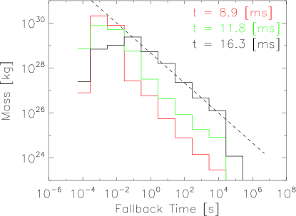
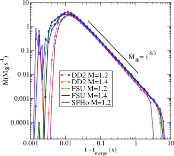
Figure 31: Left: Mass distribution as a function of the fallback time predicted from data of a simulation for a binary with $Q=5$, $\chi=0.5$ and $\mathcal{C}=0.1$ ($R_{\mathrm{NS}}=$20.7\text{\,}\mathrm{km}$$ for a $1.4\,M_{\odot}$ neutron star) modeled by a $\Gamma=2$ polytrope at different times. The dashed line shows expected $t^{-2/3}$ behavior. Right: Mass fallback rate predicted from data of simulations for various black hole–neutron star binaries. Images repoduced with permission from [left] Chawla et al. (2010); and [right] from Brege et al. (2018), copyright by APS.

Figure 31 generated by Chawla et al. (2010) (left) and Brege et al. (2018) (right) shows the mass fallback rate right after tidal disruption in black hole–neutron star binaries for various systems. The fallback rate is found to obey the power law in time of $\propto t^{-5/3}$ irrespective of the models. This time dependence coincides with that of tidal disruption events of stars in marginally unbound orbits around supermassive black holes (Rees, 1988; Phinney, 1989). Normalization of the fallback rate depends significantly on the binary system, and $\sim 0.001$–$0.01\,M_{\odot}\,${\mathrm{s}}^{-1}$(t/$1\text{\,}\mathrm{s}$)^{-5/3}$ may reasonably be expected for the case in which significant tidal disruption occurs (Kyutoku et al., 2015; Brege et al., 2018).

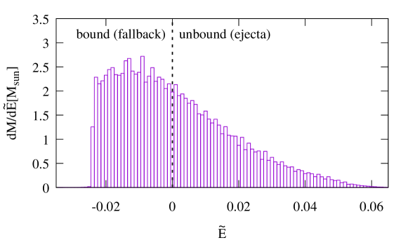
Figure 32: Mass distribution as a function of the specific energy of material remaining outside the black hole at $10\text{\,}\mathrm{ms}$ after the onset of merger for a binary with $M_{\mathrm{BH}}=4.05\,M_{\odot}$, $\chi=0.75$, $M_{\mathrm{NS}}=1.35\,M_{\odot}$ and $R_{\mathrm{NS}}=$13.6\text{\,}\mathrm{km}$$ ($Q=3$, $\mathcal{C}=0.147$) modeled by a piecewise-polytropic approximation of the H4 equation of state (Glendenning and Moszkowski, 1991; Lackey et al., 2006). Components with $\tilde{E}<0$ and $\tilde{E}>0$ represent bound and unbound material, respectively. The material within $200\text{\,}\mathrm{km}$ around the central black hole is removed from the plot assuming that it represents an accretion disk. This figure is generated from data of Kyutoku et al. (2015)

As we stated in Sect. 3.3, coalescences of circular compact binaries in bound orbits are fundamentally different from tidal disruption events associated with hyperbolic encounters. Thus, it is not expected a priori that the fallback rate is given by a power law with the index of $-5/3$. A key ingredient for realizing this index is that the mass of fallback material is distributed uniformly with respect to the specific energy, $\tilde{E}$ (Rees, 1988). Actually, the uniform distribution is found to be approximately realized for bound material with $\tilde{E}<0$ in black hole–neutron star binaries. Figure 32 shows the distribution at $10\text{\,}\mathrm{ms}$ after the onset of merger for a typical system. We exclude material within $200\text{\,}\mathrm{km}$ around the remnant black hole from this plot considering that they approximately correspond to disk components, and the disk outflow is also absent in this simulation. While the amount of dynamical ejecta with $\tilde{E}>0$ decreases as $\tilde{E}$ increases, the fallback material with $\tilde{E}<0$ exhibits an approximately flat profile, resulting in the approximate $t^{-5/3}$ fallback rate. The mechanism that realizes this distribution has not been clarified yet, and it would be worthwhile to study this topic in more detail (see, e.g., Lodato et al. 2009 for a study on tidal disruption events).

Because the disk outflow is launched at some point after disk formation (see Sect. 3.5.2), a part of it will prevent fallback of the material at late times. Furthermore, mass ejection from the remnant disk itself could produce additional fallback material. The realistic fallback rate and relevance to observable features will be determined by interaction of various components. In addition, r-process heating also modifies the fallback rate (Metzger et al., 2010a; Desai et al., 2019; Ishizaki et al., 2021). They need further investigations.

3.4.5 Dynamical ejecta

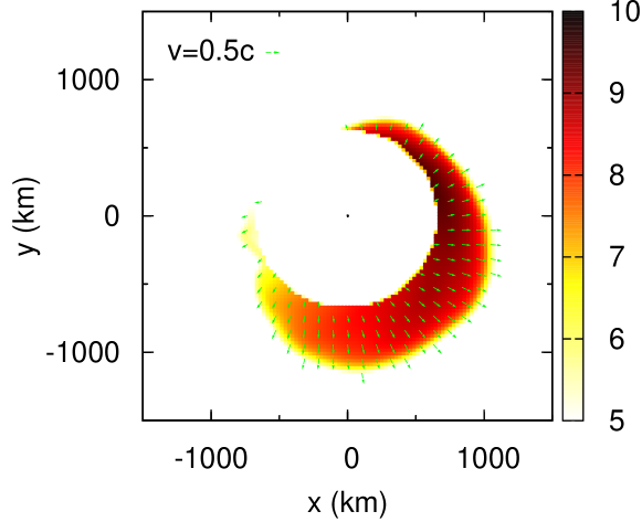
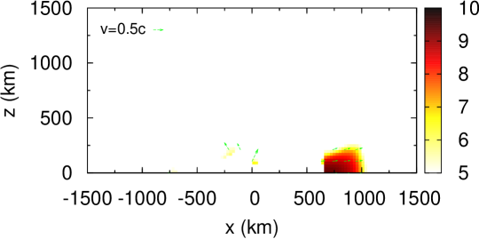
Figure 33: Profile of the rest-mass density and the velocity of the unbound material on the equatorial plane (top) and the meridional plane (bottom) at $10\text{\,}\mathrm{ms}$ after the onset of merger for a binary with $M_{\mathrm{BH}}=4.05\,M_{\odot}$, $\chi=0.75$, $M_{\mathrm{NS}}=1.35\,M_{\odot}$, and $R_{\mathrm{NS}}=$13.6\text{\,}\mathrm{km}$$ ($Q=3$, $\mathcal{C}=0.147$) modeled by a piecewise-polytropic approximation of the H4 equation of state (Glendenning and Moszkowski, 1991; Lackey et al., 2006). Image reproduced with permission from Kyutoku et al. (2013), copyright by APS.

Dynamical ejecta from black hole–neutron star binaries are generated from the outermost part of the tidal tail and characterized by the high degree of nonsphericity (Kyutoku et al., 2013). Figure 33 illustrates the rest-mass density of only unbound material at $10\text{\,}\mathrm{ms}$ after the onset of merger for a representative case. The dynamical ejecta typically take a crescent-like shape on the equatorial plane at this instant as long as the degree of tidal disruption is significant. Quantitatively, they sweep out only about a half of the orbital plane and are concentrated around the plane with a half opening angle of $\sim$$$–$20\mathrm{°}$ (Kyutoku et al., 2013; Foucart et al., 2017; Brege et al., 2018). Anisotropy of mass ejection is ascribed to the (not independent) facts that (i) black hole–neutron star binaries are completely asymmetric systems in terms of the profile of material and (ii) dynamical mass ejection in black hole–neutron star binaries is driven primarily by tidal torque, which is most efficient in the direction along the orbital plane. This morphology should be contrasted with more spherical dynamical ejecta from binary neutron stars, especially equal-mass systems (see, e.g., Hotokezaka et al., 2013b). The opening angles depend only weakly on the equation of state except for the cases in which tidal disruption occurs only marginally (Kyutoku et al., 2015), and we present its simplified explanation in Appendix C.2.

Anisotropic mass ejection may induce various potentially-observable features (Kyutoku et al., 2013, 2015). Possible effects on electromagnetic emission are discussed later in Sect. 4.1. One kinematic consequence is recoil motion of the remnant black hole (see Rosswog et al. 2000 for early discussions in the case of asymmetric binary neutron stars). Because the dynamical ejecta escape from the system carrying a net linear momentum with a typical center-of-mass velocity of $0.1$–$0.2c$, the remnant black hole obtains the recoil velocity in the direction opposite to the ejecta. The center-of-mass velocity of the remnant black hole may become as high as $\sim$1000\text{\,}\mathrm{km}\text{\,}{\mathrm{s}}^{-1}$$, particularly if the system experiences significant tidal disruption. We note that significant tidal disruption suppresses gravitational-wave recoil (Shibata et al., 2009), which might be efficient in the final plunge phase in the absence of tidal disruption (Wiseman, 1992; Blanchet et al., 2005).

As they escape from the gravitational binding of the remnant black hole, the expansion of the dynamical ejecta gradually becomes homologous (Kyutoku et al., 2015). In the course of this transition, the crescent-like shape should change to a half-disk-like shape, because the inner region is decelerated further by the influence of a deep gravitational potential. The morphology of the ejecta may also be modified by the radioactive decay heat of r-process elements (Darbha et al., 2021, see also Rosswog et al. 2014 for binary neutron stars in Newtonian gravity). To derive precise observational features related to the ejecta morphology, (not necessarily fully general relativistic) longterm evolution for $1$–$10\text{\,}\mathrm{s}$ is necessary. On a long time scale of $10$–$100\text{\,}\mathrm{y}\mathrm{r}$ which depends not only on the ejecta property but also on the density of the interstellar medium, the dynamical ejecta as well as the disk outflow (see Sect. 3.5.2) are decelerated by the interstellar medium and eventually dissolve into it (Nakar and Piran, 2011).

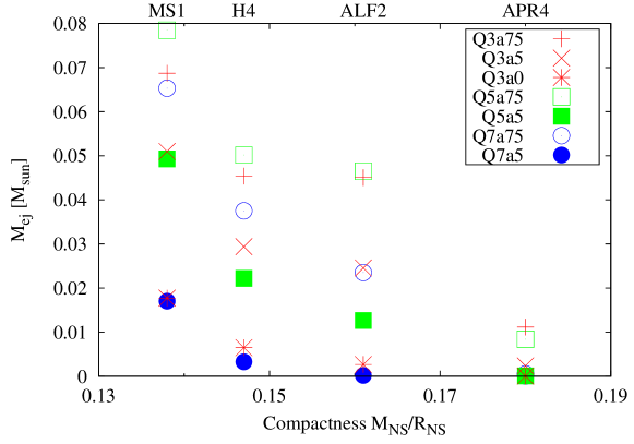
Figure 34: Mass of the dynamical ejecta for various black hole–neutron star binaries with $M_{\mathrm{NS}}=1.35\,M_{\odot}$. The horizontal axis is the compactness of the neutron star, and corresponding equations of state are written above the top axis. The legend indicates the mass ratio and the spin parameter of the black hole, e.g., Q5a75 means $Q=5$ and $\chi=0.75$. Image reproduced with permission from Kyutoku et al. (2015), copyright by APS.

Dynamical ejecta from black hole–neutron star binaries can take a wide range of mass depending on binary parameters (Kyutoku et al., 2015). Figure 34 displays the mass of the dynamical ejecta, $M_{\mathrm{ej}}$, for various black hole–neutron star binaries. If tidal disruption does not occur, the ejecta mass is essentially zero. This is a typical outcome for binaries with a high mass ratio, a low black-hole spin, and/or a large neutron-star compactness such as those detected by and/or reported with gravitational waves during the LIGO-Virgo O3 (Abbott et al., 2021a, b). By contrast, the mass can easily exceed $0.01\,M_{\odot}$ if tidal disruption is significant. Notably, Lovelace et al. (2013) reported that $(0.26\pm 0.16)\,M_{\odot}(1.4\,M_{\odot}/M_{\mathrm{NS}})$ may be ejected from a system with $Q=3$, $\mathcal{C}=0.144$ modeled by a $\Gamma=2$ polytrope, and a very high black-hole spin of $\chi=0.97$. These large values should be compared with dynamical ejecta from binary neutron stars, whose mass is limited to $\lesssim 0.02\,M_{\odot}$ (see Hotokezaka et al., 2013b; Sekiguchi et al., 2015, 2016; Kiuchi et al., 2019; Vincent et al., 2020, for reports of $\gtrsim 0.01\,M_{\odot}$) unless the mass ratio is higher than an extreme value (as binary neutron stars) of $\approx 1.5$ (Dietrich et al., 2017b).

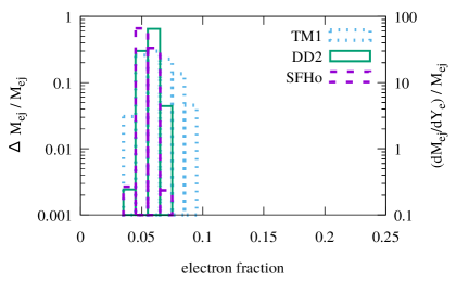
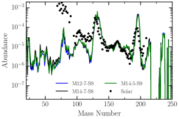
Figure 35: Left: Mass distribution as a function of the electron fraction in the dynamical ejecta for binaries with $M_{\mathrm{BH}}=5.4\,M_{\odot}$, $\chi=0.75$, and $M_{\mathrm{NS}}=1.35\,M_{\odot}$ ($Q=4$). Adopted equations of state are SFHo (Steiner et al., 2013), DD2 (Banik et al., 2014), and TM1 (Hempel et al., 2012), with which the radii of $1.35\,M_{\odot}$ neutron stars are $11.9$, $13.2$, and $14.5\text{\,}\mathrm{km}$, respectively. The simulations are performed incorporating neutrino irradiation. Right: Abundance pattern of the r-process nucleosynthesis in dynamical ejecta from various models of black hole–neutron star binaries simulated in Deaton et al. (2013); Foucart et al. (2014). Neutrino irradiation is taken into account by a post process, and it does not change the results appreciably. Images reproduced with permission from [left] Kyutoku et al. (2018), copyright by APS; and [right] Roberts et al. (2017), copyright by the authors.

Because the shock interaction plays only a minor role in the ejection process, the dynamical ejecta keep extreme neutron richness of the cold neutron star (Deaton et al., 2013; Foucart et al., 2014, 2017; Kyutoku et al., 2018; Brege et al., 2018; Foucart et al., 2019b). The left panel of Fig. 35 shows the mass distribution as a function of the electron fraction for simulations with neutrino irradiation (Kyutoku et al., 2018). This figure shows that the electron fraction is as low as $Y_{\mathrm{e}}\approx 0.05$–$0.1$ preserving original values of the neutron-star material even if the neutrino irradiation is taken into account in numerical simulations. This should again be compared with the dynamical ejecta from binary neutron stars, the range of whose electron fraction can be extended up to $Y_{\mathrm{e}}\approx 0.4$ by the shock heating and associated weak interactions, i.e., electron/positron captures and neutrino irradiation (Sekiguchi et al., 2015; Palenzuela et al., 2015; Foucart et al., 2016a; Sekiguchi et al., 2016; Radice et al., 2016; Lehner et al., 2016; Bovard et al., 2017; Radice et al., 2018; Vincent et al., 2020). There are two reasons for this significant difference. First, because the dynamical ejecta from black hole–neutron star binaries do not experience significant shock heating, the temperature is kept so low that the electron/positron pairs are not efficiently produced. Second, the dynamical ejecta are located at the distant region when the circularized accretion disk starts to emit a copious amount of neutrinos. Thus, the neutrino flux is low when neutrinos catch up the dynamical ejecta. These two facts do not allow the dynamical ejecta to increase the electron fraction. As a minor effect, equations of state that predict small neutron-star radii tend to give slightly low electron fraction. This correlation may stem from the correlation between the symmetry energy of the nuclear matter and the radius of the neutron star (Lattimer and Prakash, 2001).

The low electron fraction of the dynamical ejecta indicates that the yield of subsequent nucleosynthesis is dominated by heavy r-process elements with the mass number $\gtrsim 130$, i.e., beyond the second peak. This expectation is confirmed in the right panel of Fig. 35 generated by Roberts et al. (2017), which shows the abundance pattern of the nucleosynthesis for selected models of black hole–neutron star binaries. The abundance pattern is robust against variation of binary parameters, although the detailed features depend on nuclear physics inputs (see, e.g., Mendoza-Temis et al., 2015; Mumpower et al., 2016; Wu et al., 2016; Zhu et al., 2021).

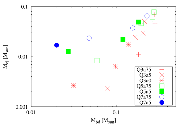
Figure 36: Comparison between the mass of the dynamical ejecta, $M_{\mathrm{ej}}$, and that of the bound material, $M_{\mathrm{bd}}$, which may be regarded as the disk mass. The mass of the neutron star $M_{\mathrm{NS}}$ is fixed to be $1.35\,M_{\odot}$. The legend indicates the mass ratio and the spin parameter of the black hole, e.g., Q5a75 means $Q=5$ and $\chi=0.75$. Equations of state are varied for given values of $Q$ and $\chi$. Image reproduced with permission from Kyutoku et al. (2015), copyright by APS.

One intriguing question may be as follows: “Do the dynamical ejecta or the disk outflow dominate the mass of the ejected material?” This is important for understanding abundance of r-process elements and emission features of the kilonova/macronova for black hole–neutron star binaries (see also Sect. 3.5). In the case of binary neutron stars, it is strongly believed that the disk outflow dominates the dynamical ejecta from theoretical calculations and observations of AT 2017gfo (see, e.g., Kasen et al., 2017; Shibata et al., 2017a; Perego et al., 2017; Villar et al., 2017).

The answer for black hole–neutron star binaries may be that it depends on the mass ratio. Figure 36 compares the mass of the dynamical ejecta with that of the remnant disk for various systems with $M_{\mathrm{NS}}=1.35\,M_{\odot}$. This figure indicates that the mass of the dynamical ejecta is correlated with that of the bound material in a manner dependent on the mass ratio for a parameter range depicted here, specifically $3\leq Q\leq 7$. It should be cautioned that, however, the neutron-star mass is not varied in Fig. 36. In fact, most simulations of black hole–neutron star binaries have focused on the plausibly typical value of $M_{\mathrm{NS}}\lesssim 1.35$–$1.4\,M_{\odot}$ to date. Further investigations are required to reveal precise dependence on binary parameters (Foucart et al., 2014). In particular, high mass-ratio systems with $Q>7$ should also be investigated systematically. Accordingly, the following discussions need to be understood with this caveat in mind.

For high mass-ratio systems $Q\gtrsim 5$, the mass of the dynamical ejecta depends relatively weakly on the mass of the disk. For example, they become comparable at $M_{\mathrm{bd}}\approx M_{\mathrm{ej}}\approx 0.02\,M_{\odot}$ for $Q=7$. Presuming that $\sim 30\%$ could be ejected from the remnant disk (see Sect. 3.5.2), dynamical mass ejection could be a dominant mechanism for black hole–neutron star binaries with $Q\gtrsim 7$, particularly for the case in which the tidal disruption is moderate (that is, the amount of material remaining outside the black hole is not very large). As we will discuss later in Sect. 3.5.2, the realistic fraction of the material ejected from the remnant disk is estimated to be 15%–30% from various simulations.

As the mass ratio decreases, the fraction of the disk outflow increases. Figure 36 shows that the mass of the dynamical ejecta is typically only $\sim 5\%$–20% of the disk mass for $Q\sim 3$–$5$. Thus, it is likely that the amount of the disk outflow becomes comparable to that of the dynamical ejecta. This trend is enhanced for the regime of very-low-mass black holes, or equivalently, very low mass ratios. The mass of the dynamical ejecta decreases to $\lesssim${10}^{-3}$\,M_{\odot}$ for nonspinning black holes with $Q\lesssim 3$ (Foucart et al., 2019b; Hayashi et al., 2021; Most et al., 2021a), although the remnant disk can be as massive as $\sim 0.05$–$0.1\,M_{\odot}$. For these systems, the disk outflow will dominate the amount of the ejected material.

The mass ratio also governs the average velocity of the dynamical ejecta, although significant dispersion is found associated with variations of other binary parameters (Kyutoku et al., 2015; Foucart et al., 2017; Hayashi et al., 2021). Here, the average velocity is defined from the kinetic energy, $T_{\mathrm{kin}}$, and the mass, $M_{\mathrm{ej}}$, by $\sqrt{2T_{\mathrm{kin}}/M_{\mathrm{ej}}}$. Quantitatively, the asymptotic velocity is as high as $\sim 0.2c$ for high mass-ratio systems with $Q\sim 5$–$7$, for which corresponding kinetic energy reaches $\sim${10}^{52}\text{\,}\mathrm{e}\mathrm{r}\mathrm{g}$$. As the mass ratio decreases to $Q\lesssim 1.5$, the asymptotic velocity decreases to $\sim 0.1c$ and the kinetic energy decreases by orders of magnitude due to the small value of the ejecta mass (Foucart et al., 2019b; Hayashi et al., 2021).

Figure 37: Mass distribution as a function of the velocity of the dynamical ejecta measured at $10\text{\,}\mathrm{ms}$ after the onset of merger for various black hole–neutron star binaries. The distribution is normalized by the total mass of the ejecta. It should be cautioned that Fig. 32 is drawn with respect to the specific energy instead of the velocity used here. Although this figure is derived by analyzing only the material on the equatorial plane, the conclusion remains the same even if all the dynamical ejecta are taken into account (Brege et al., 2018; Most et al., 2021a). Image reproduced with permission from Kyutoku et al. (2015), copyright by APS.

The velocity of the dynamical ejecta is distributed approximately symmetrically about the averaged value and does not extend to high velocity of $\gtrsim 0.5c$ (Kyutoku et al., 2015; Brege et al., 2018; Most et al., 2021a, see also Rosswog et al. 2013 for early Newtonian work). Figure 37 shows the mass distribution as a function of the velocity for various black hole–neutron star binaries (Kyutoku et al., 2015), which is directly related to the $\tilde{E}>0$ side of Fig. 32. The cutoff features on the highest-velocity side in these distributions are distinct from the so-called fast tail found in binary-neutron-star mergers, which may extend to $\gtrsim 0.8c$ (Hotokezaka et al., 2013b, 2018; Radice et al., 2018). This difference may be reflected in electromagnetic counterparts, particularly in the early part of kilonova/macronova remnants as we discuss in Sect. 4. We note that, although Fig. 37 is derived by analyzing only the material on the equatorial plane, the conclusion remains the same even if all the dynamical ejecta are taken into account (Brege et al., 2018; Most et al., 2021a).

Fitting formulae for the mass of the dynamical ejecta are provided by Kawaguchi et al. (2016); Krüger and Foucart (2020), where Kawaguchi et al. (2016) also derive a formula for the velocity. A fitting formula for the disk outflow is also proposed based on the fitting formulae for the mass of the material remaining outside the black hole and for the dynamical ejecta (Raaijmakers et al., 2021), while the efficiency of the ejection depends on the mass and the compactness of the disk and thus is highly uncertain (see Sect. 3.5.2).

3.5 Postmerger activity

The remnant disk is considered to evolve via neutrino emission and magnetohydrodynamical turbulence on a long viscous time scale. In a wide range of astrophysics studies, the kinematic shear viscosity $\nu$ in the accretion disk is often parametrized by the so-called alpha parameter $\alpha_{\nu}$ as (Shakura and Sunyaev, 1973)

$$\nu=\alpha_{\nu}c_{s}H,$$ (42)

where $c_{s}$ and $H$ are the sound speed and the scale height of the disk, respectively. The value of $\alpha_{\nu}$ is believed to be determined by magnetohydrodynamical processes as we describe in Sect. 3.5.3, and recent studies suggest $\alpha_{\nu}\approx 0.01$–$0.1$ is reasonable (Fernández et al., 2019; Christie et al., 2019). If we presume such values of $\alpha_{\nu}$, the viscous time scale is estimated by

$$t_{\mathrm{vis}}:=\frac{R^{2}}{\nu}\approx$0.33\text{\,}\mathrm{s}$\pqty{\frac{\alpha_{\nu}}{0.03}}^{-1}\pqty{\frac{c_{s}}{0.1c}}^{-1}\pqty{\frac{H/R}{1/3}}^{-1}\pqty{\frac{R}{$100\text{\,}\mathrm{km}$}},$$ (43)

where $R$ is the cylindrical radius of the disk. This is much longer than the dynamical time scale of the disk,

$$t_{\mathrm{dyn}}:=2\pi\sqrt{\frac{R^{3}}{GM_{\mathrm{BH,f}}}}=$5.5\text{\,}\mathrm{ms}$\pqty{\frac{R}{$100\text{\,}\mathrm{km}$}}^{3/2}\pqty{\frac{M_{\mathrm{BH,f}}}{10\,M_{\odot}}}^{-1/2}.$$ (44)

Furthermore, $t_{\mathrm{vis}}$ becomes even longer for an outer region of the disk. This comparison indicates that a longterm simulation of $\order{1}$\mathrm{s}$\gg t_{\mathrm{dyn}}$ is required for understanding the evolution of the accretion disk. Because the evolution is also governed by neutrino emission, implementation of neutrino transfer is another key ingredient for quantitative exploration. These facts make the physical postmerger simulation computationally challenging.

To date, only a few work have reported longterm simulations of an accretion disk surrounding a black hole in full general relativity i.e., numerical relativity, (Shibata and Sekiguchi, 2012; Foucart et al., 2015; Fujibayashi et al., 2020a, b; Most et al., 2021b), although many work have been done in (pseudo-)Newtonian gravity (Setiawan et al., 2004; Lee et al., 2005; Setiawan et al., 2006; Fernández and Metzger, 2013; Just et al., 2015; Fernández et al., 2020) or with adopting a fixed background spacetime (Shibata et al., 2007; Siegel and Metzger, 2017, 2018; Fernández et al., 2019; Miller et al., 2019a; Christie et al., 2019), in some cases starting with initial conditions taken from merger simulations (Cowling approximation; Hossein Nouri et al., 2018). In this Sect. 3.5, we review the current status of our understanding for neutrino emission, the disk outflow powered by the viscous heating, and the effect of magnetic fields, focusing on the results obtained by fully general-relativistic simulations. We caution that magnetohydrodynamics simulations in numerical relativity as long as $1\text{\,}\mathrm{s}$ have not been reported and are needed for robust understanding of the postmerger evolution in the future (see Most et al., 2021b, for a recent simulation up to $\sim$350\text{\,}\mathrm{ms}$$).

3.5.1 Neutrino emission

The hot and massive remnant accretion disk emits a copious amount of neutrinos primarily via electron/positron captures onto nucleons (Deaton et al., 2013; Foucart et al., 2014; Kyutoku et al., 2018, see also Janka et al. 1999 for pioneering study in Newtonian gravity). If a massive accretion disk of $\gtrsim 0.1\,M_{\odot}$ is formed around a rapidly spinning black hole with $\lesssim 10\,M_{\odot}$, the luminosity reaches $\gtrsim${10}^{53}\text{\,}\mathrm{e}\mathrm{r}\mathrm{g}\,\mathrm{s}^{-1}$$ at $\approx$10\text{\,}\mathrm{ms}$$ after the onset of merger, when the tidal tail collides with itself and forms a remnant disk. The order of the peak luminosity is the same as that found for stellar core collapse and binary-neutron-star mergers. The emission efficiency is a few to several percent of the accretion rate onto the black hole for a disk with the maximum rest-mass density of $\gtrsim${10}^{11}\text{\,}\mathrm{g}\text{\,}{\mathrm{cm}}^{-3}$$ and increases as the spin parameter of the remnant black hole increases (Fujibayashi et al., 2020a, b). Because the optical depth of the disk to neutrinos can exceed unity (see, e.g., Deaton et al. 2013; Foucart et al. 2015; Hossein Nouri et al. 2018), the neutrino luminosity is saturated to $\sim${10}^{53}\text{\,}\mathrm{e}\mathrm{r}\mathrm{g}\,\mathrm{s}^{-1}$$ in the early stage of the postmerger evolution until the disk becomes optically thin to neutrinos as a result of the accretion onto the black hole (see also Lee et al., 2005; Setiawan et al., 2006).

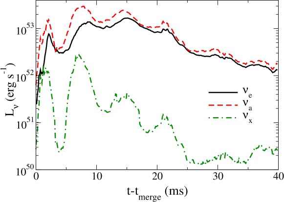
Figure 38: Time evolution of the luminosity for electron neutrinos ($\nu_{\mathrm{e}}$: black solid), electron antineutrinos ($\nu_{\mathrm{a}}$: red dashed), and one of the other neutrinos ($\nu_{\mathrm{x}}$: green dot-dashed), for the same model as that shown in Fig. 30. The disk mass at $20\text{\,}\mathrm{ms}$ after the onset of merger is reported to be $0.08\,M_{\odot}$. The mass and the spin parameter of the remnant black hole are $8.00\,M_{\odot}$ and $0.87$, respectively. Image reproduced with permission from Foucart et al. (2014), copyright by APS.

Among the six species of neutrinos, electron antineutrinos always carry away the largest amount of energy. Figure 38 generated by Foucart et al. (2014) shows a typical example of luminosity evolution in an early stage of the postmerger accretion disk (Foucart et al., 2014). Quantitatively, the peak luminosity of electron antineutrinos typically reaches $\gtrsim${10}^{53}\text{\,}\mathrm{e}\mathrm{r}\mathrm{g}\,\mathrm{s}^{-1}$$ if the accretion disk with $\gtrsim 0.1\,M_{\odot}$ is formed, and it is higher than the luminosity of electron neutrinos by a factor of $\sim 2$.

The reasons for the dominance of electron antineutrinos are twofold, and both are ascribed to the neutron-rich composition of the remnant disk inherited from the neutron star. First, the number of capture reactions is larger for positrons than for electrons, because the remnant disk equilibrates toward a protonized state from a neutron-rich state. Second, the neutron-rich disk is optically thicker to electron neutrinos than to electron antineutrinos. This feature puts the neutrinosphere (an analog of the photosphere for photons) for electron antineutrinos at high-temperature regions close to the midplane of the disk. Thus, the number of emitted neutrinos is larger and the energy of individual neutrinos is higher for electron antineutrinos than for electron neutrinos. The dominance in number should be contrasted with neutrino emission from core-collapse supernovae, in which electron neutrinos are larger in number than electron antineutrinos due to continuous deleptonization. This difference may introduce differences in neutrino oscillations such as matter-neutrino resonances (Malkus et al., 2012, see also the end of this Sect. 3.5.1). Muon and tau neutrinos and their antineutrinos, denoted collectively by “x” neutrinos in the context of stellar core collapse and compact binary mergers, are typically dimmer by more than an order of magnitude than two dominant species. This is because the x neutrinos are emitted only via neutral-current processes and the temperature of the disk is relatively low as described in Sect. 3.4.3.

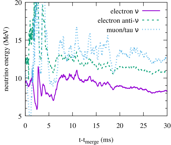
Figure 39: Time evolution of the average energy of electron neutrinos (purple solid), electron antineutrinos (green dashed), and other neutrinos (cyan dotted) for a binary with $M_{\mathrm{BH}}=5.4\,M_{\odot}$, $\chi=0.75$, $M_{\mathrm{NS}}=1.35\,M_{\odot}$, $R_{\mathrm{NS}}=$13.2\text{\,}\mathrm{km}$$ ($Q=4$, $\mathcal{C}=0.151$) modeled by the DD2 equation of state (Banik et al., 2014). This figure is generated from data of Kyutoku et al. (2018).

More precisely, the energy of individual neutrinos is the lowest for electron neutrinos, the middle for electron antineutrinos, and the highest for x neutrinos. Quantitatively, for example in the case of $M_{\mathrm{BH}}=5.4\,M_{\odot}$, $\chi=0.75$, and $M_{\mathrm{NS}}=1.35\,M_{\odot}$ ($Q=4$) shown in Fig. 39, the average values of the energy for electron neutrinos, electron antineutrinos, and x neutrinos are $8$, $11$, and $13\text{\,}\mathrm{MeV}$, respectively, at $20\text{\,}\mathrm{ms}$ after the onset of merger, depending weakly on the equation of state (Kyutoku et al., 2018). The average values of neutrino energy owe their hierarchy to the optical depth of the disk to each species of neutrinos described above. That is, the average values reflect the location and the temperature of the neutrinosphere for each species. We caution that the energy of neutrinos is derived only approximately by the total energy and number of neutrinos in these simulations. Quantitative estimation of the neutrino energy requires a multienergy transport scheme, which has never been adopted in simulations of black hole–neutron star binaries. Studies such as the one conducted by Foucart et al. (2020) for binary neutron stars are necessary.

The peak neutrino luminosity does not always increase with the increase of the disk mass, because the temperature can be lower for a more massive disk (Kyutoku et al., 2018). As we discussed in Sect. 3.4.2, the disk mass is smaller for a more compact neutron star if the other binary parameters are fixed. However, as we discussed in Sect. 3.4.3, the temperature tends to be higher for a more compact neutron star, because tidal disruption occurs at an orbit closer to the black hole, and reflecting higher velocity at the closer orbit, the shock interaction results in higher temperature. As the emission rate of energy via the electron/positron capture is approximately proportional to $T^{6}$ (Fuller et al., 1985), the temperature, $T$, plays a more decisive role in neutrino emission than the disk mass or the rest-mass density.

To date, no inspiral-merger-postmerger simulation in neutrino-radiation hydrodynamics has incorporated well-resolved magnetohydrodynamical or viscous heating of the disk, and thus the luminosity for $\gtrsim$10\text{\,}\mathrm{ms}$$ after the onset of merger is likely to be underestimated (but see also Most et al., 2021a, b, for the effort). In reality, longterm neutrino emission is controlled by magnetically-induced viscous heating, which compensates the neutrino cooling (Lee et al., 2005; Setiawan et al., 2006). Magnetohydrodynamics simulations in the Cowling approximation found that magnetically-induced turbulent viscosity enhances the neutrino luminosity by a factor of $\sim 2$ for initial $\sim$50\text{\,}\mathrm{ms}$$ if the magnetic-field strength is $\gtrsim${10}^{15}\text{\,}\mathrm{G}$$ at the maximum inside the accretion disk (Hossein Nouri et al., 2018). Further longterm simulations have been performed in viscous-hydrodynamics numerical-relativity simulations in axisymmetry, which are described in Sect. 3.5.2 with a particular emphasis on the disk outflow (Fujibayashi et al., 2020a, b). Generally speaking, the neutrino luminosity is higher than ${10}^{53}\text{\,}\mathrm{e}\mathrm{r}\mathrm{g}\,\mathrm{s}^{-1}$ only in the initial $10$–$100\text{\,}\mathrm{ms}$ and decreases to $\lesssim${10}^{50}\text{\,}\mathrm{e}\mathrm{r}\mathrm{g}\,\mathrm{s}^{-1}$$ at $\sim$1\text{\,}\mathrm{s}$$ after the disk formation, because the time scale of the weak interaction becomes too long due to the viscous disk expansion. Thus, it is not very likely that neutrino pair annihilation (Rees and Meszaros, 1992, see also the next paragraph) can drive an ultrarelativistic jet for the entire duration of short-hard gamma-ray bursts, which is typically $0.1$–$1\text{\,}\mathrm{s}$ (see, e.g., Nakar 2007; Berger 2014 for reviews), in black hole–neutron star binary coalescences. It should also be noted that neutrino-driven winds have not been observed in numerical-relativity simulations without viscosity (Kyutoku et al., 2018). Neutrino absorption is not found to enhance the mass of the viscous disk outflow, either, in numerical-relativity simulations with viscosity (Fujibayashi et al., 2020a).

We should mention two neutrino processes that have never been incorporated in numerical-relativity simulations of black hole–neutron star binaries as a topic for future investigations. One is the neutrino pair annihilation, which could power an ultrarelativistic jet (Mochkovitch et al., 1993; Janka et al., 1999; Birkl et al., 2007; Zalamea and Beloborodov, 2011). Although this process may be handled semiquantitatively within the moment formalism (Fujibayashi et al., 2017, 2018), solving Boltzmann’s equation directly will be valuable for incorporating precise angular dependence of neutrinos (see, e.g., Cardall et al. 2013; Shibata et al. 2014 for approaches in numerical relativity). Monte-Carlo neutrino-radiation transport is also useful to incorporate pair annihilation (Foucart et al., 2020). The other is the neutrino oscillation, which could modify nucleosynthetic yields for some part of the ejecta (Malkus et al., 2012, 2016; Wu and Tamborra, 2017; Wu et al., 2017; Padilla-Gay et al., 2021; Li and Siegel, 2021). Its modeling will require us to address the challenging task of solving quantum kinetic equations in a dynamical spacetime (see, e.g., Richers et al. 2019 for relevant work). The so-called fast flavor conversion is partially incorporated in a disk simulation in a fixed, Kerr background (Li and Siegel, 2021).

3.5.2 Disk outflow

The long time scale of $\gtrsim$1\text{\,}\mathrm{s}$$ for the evolution of the remnant disk makes its accurate simulation a challenging task. In particular, because magnetohydrodynamic instabilities are often characterized by a short wavelength and magnetohydrodynamical turbulence can be maintained only in three-dimensional simulations (see Balbus and Hawley 1998 for reviews), the computational cost is extremely high if we try to study the longterm evolution of the remnant disk by magnetohydrodynamics simulations irrespective of whether the gravity is Newtonian or relativistic. To save computational costs, it is customary to adopt viscous hydrodynamics with a value of $\alpha_{\nu}$ chosen phenomenologically to reproduce results of high-resolution magnetohydrodynamics simulations. Here, we need to keep in mind that this prescription does not reproduce all of the magnetohydrodynamical effects in a faithful manner (see also the final paragraph of Sect. 3.5.2).

Numerical-relativity simulations of black hole–accretion disk systems have recently been performed in two-dimensional, axisymmetric neutrino-radiation viscous hydrodynamics (Fujibayashi et al., 2020a, b). Initial conditions of these work are given by an axisymmetric equilibrium disk surrounding a black hole (Shibata, 2007). While the entropy per baryon is taken to be constant throughout the disk, the profiles of the angular momentum and the electron fraction are modeled by functions motivated by results of inspiral-merger-postmerger simulations of black hole–neutron star binaries in neutrino-radiation hydrodynamics (Kyutoku et al., 2018). The equation of state is given by the DD2 equation of state for high density (Banik et al., 2014) and by the Helmholtz equation of state for low density (Timmes and Swesty, 2000). In the following, we describe properties of the viscous disk outflow investigated in Fujibayashi et al. (2020a, b, see also for pioneering pseudo-Newtonian simulations). We focus mainly on the results for the fiducial value of $\alpha_{\nu}=0.05$.

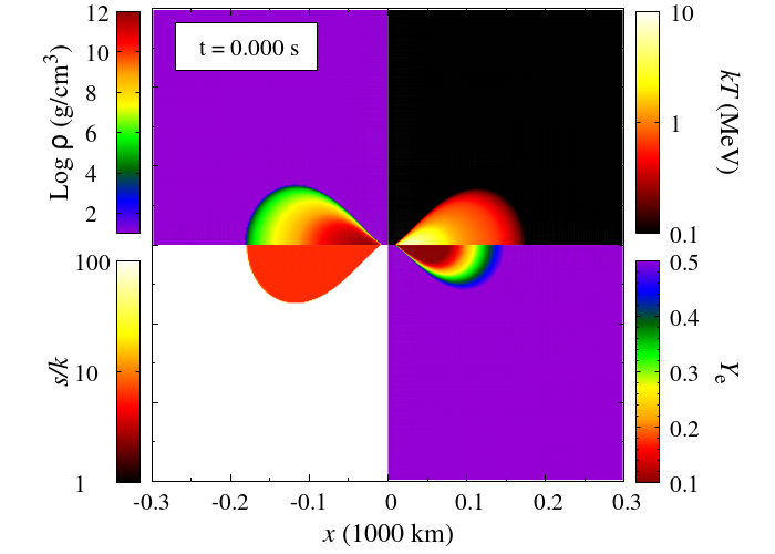
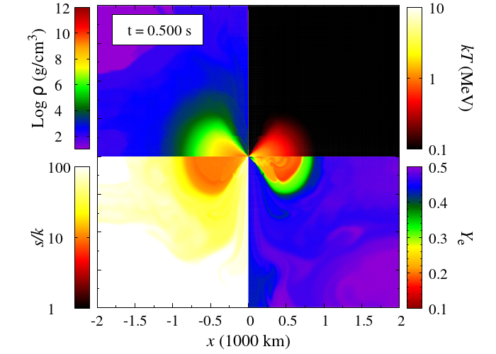
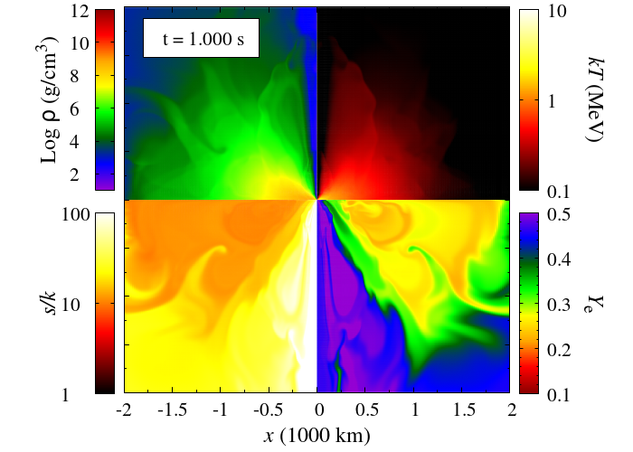
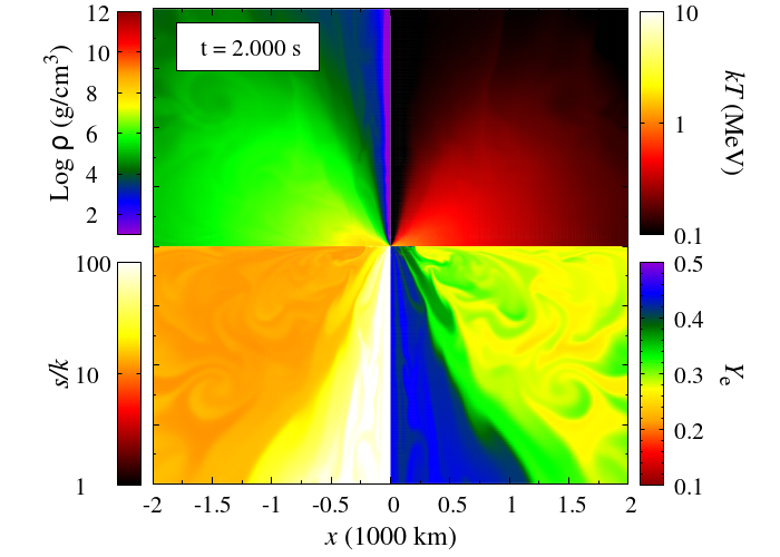
Figure 40: Profile of the rest-mass density (left top), the temperature in units of $\mathrm{MeV}$ (right top), the entropy per baryon in units of the Boltzmann constant (left bottom), and the electron fraction (right bottom) at $1\text{\,}\mathrm{s}$ (left) and $2\text{\,}\mathrm{s}$ (right) after the start of viscous evolution for a $0.1\,M_{\odot}$ disk surrounding a $3\,M_{\odot}$ black hole with $\chi=0.8$. The size of the drawing area is $300\text{\,}\mathrm{m}$ for the left top panel and $2\text{\,}\mathrm{km}$ for the others. The alpha parameter $\alpha_{\nu}$ is taken to be $0.05$. Image reproduced with permission from Fujibayashi et al. (2020a), copyright by the authors.

In the early stage of the postmerger evolution, most of the internal energy generated by the viscous heating is consumed by the neutrino emission from the accretion disk. The viscous disk outflow is insignificant during the stage in which the neutrino cooling is efficient. As the temperature and the rest-mass density decrease due to the viscous disk expansion and the mass accretion onto the black hole, the time scale for weak interactions becomes long. Once it exceeds the viscous time scale of $\order{1}$\mathrm{s}$$, the internal energy generated by the viscous heating increases the entropy in the innermost region, because the neutrino emission becomes inefficient. As shown in Fig. 40, the entropy gradient activates convective motion so that the disk begins to expand significantly at $\approx$0.5\text{\,}\mathrm{s}$$ after the start of viscous evolution. The viscous disk outflow sets in as well due to the energy transport associated with the convection. Because the time scale of the convective motion, $\sim$10\text{\,}\mathrm{ms}$$, is much shorter than the viscous time scale, the outer part of the disk immediately gains energy once the neutrino cooling becomes inefficient.

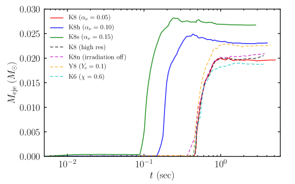
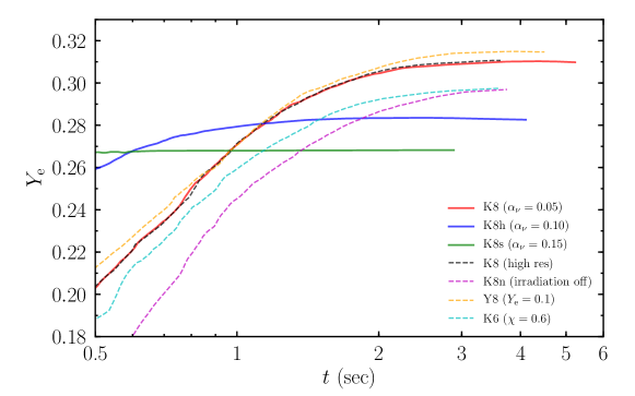
Figure 41: Time evolution of the mass (top) and the electron fraction (bottom) of the material ejected from a $0.1\,M_{\odot}$ disk surrounding a $3\,M_{\odot}$ black hole for several initial configurations and three values of $\alpha_{\nu}$. The initial radius of the disk is $\sim$180\text{\,}\mathrm{km}$$, and the spin parameter of the black hole $\chi$ is $0.8$ except for the model denoted by K6 with $\chi=0.6$. Note that the scales of the horizontal axes are different between two panels. Image reproduced with permission from Fujibayashi et al. (2020a), copyright by the authors.

The viscous outflow from the remnant disk of black hole–neutron star binary mergers typically ejects 15%–30% of the initial disk material (see also, e.g., Siegel and Metzger, 2018; Fernández et al., 2019; Christie et al., 2019; Fernández et al., 2020, for a wider range of predictions). The precise fraction of the ejected mass depends on the physical condition of the black hole–accretion disk system such as the mass and the compactness of the disk as well as the effective viscosity (Fujibayashi et al., 2020a, b). In particular, the higher viscosity, or equivalently the larger value of the alpha parameter, results in the larger fraction. The top panel of Fig. 41 shows the time evolution of the mass ejected from the system (Fujibayashi et al., 2020a). This figure shows that the amount of ejected material increases appreciably as the value of $\alpha_{\nu}$ increases (compare K8, K8h, and K8s). Thus, accurate determination of the magnitude of the kinematic viscosity is important to predict quantitatively the amount of the disk outflow. Physically, it is necessary to clarify how the magnetorotational instability enhances the turbulence (see Sect. 3.5.3).

The velocity of the viscous disk outflow is typically $0.05$–$0.1c$, depending only weakly on the physical condition of the system. This value is smaller than that for the dynamical ejecta, because this outflow is driven primarily from the outer region of the disk, where the typical velocity scale is smaller than the orbital velocity at tidal disruption during merger. The viscous disk outflow is driven nearly isotropically except for a narrow polar region, into which the angular momentum barrier prohibits the penetration of the material.

Although the black hole–accretion disk system does not host a strong neutrino emitter such as the hot and massive neutron star, the average electron fraction of the disk increases to $\expectationvalue{Y_{\mathrm{e}}}\approx 0.3$ in $t_{\mathrm{vis}}\sim$0.5\text{\,}\mathrm{s}$$ from the onset of viscous disk evolution, and the viscous disk outflow is also characterized by relatively high electron fraction if it is launched later than $t_{\mathrm{vis}}$ (see below for the discussion about the case of rapid launch). The increase of the electron fraction is ascribed to the relaxation to the equilibrium of electron/positron captures onto nucleons. Because the rest-mass density of the disk decreases to $\rho\lesssim${10}^{9}\text{\,}\mathrm{g}\text{\,}{\mathrm{cm}}^{-3}$$ prior to the launch of the outflow in this case, the degeneracy of electrons is not strong with $kT\sim$2\text{\,}\mathrm{MeV}$$ where $k$ is the Boltzmann constant. The bottom panel of Fig. 41 displays the time evolution of the average electron fraction of the ejected material and shows that the average electron fraction is higher than $0.25$ for all the cases studied in Fujibayashi et al. (2020a). Although neutrino irradiation from the disk itself helps to increase the electron fraction by $\approx 0.05$, this works only in an early evolution stage of $\lesssim$0.1\text{\,}\mathrm{s}$$ and is not a key ingredient for increasing the electron fraction of the disk outflow. This fact is found by comparing models K8 (neutrino irradiation is taken into account) and K8n (not taken into account) in the bottom panel of Fig. 41. Because the rest-mass density is lower for disks surrounding more massive black holes as we have discussed in Sect. 3.4.3, the electron fraction is even higher due to the weaker degeneracy of electrons (Fujibayashi et al., 2020b). An extensive study of the dependence of the electron fraction on various physics inputs is performed within pseudo-Newtonian gravity by Just et al. (2021).

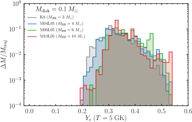
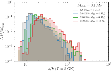
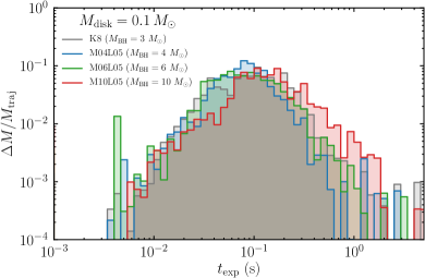
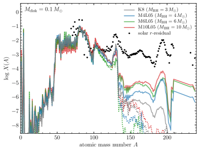
Figure 42: Mass distribution as a function of the electron fraction (left top), the entropy per baryon (right top), and the expansion time scale (left bottom) for the viscous outflow from a $0.1\,M_{\odot}$ disk with the initial radius $\sim$180\text{\,}\mathrm{km}$$ surrounding black holes with $\chi\approx 0.8$ and various masses. The alpha parameter $\alpha_{\nu}$ is taken to be $0.05$. All the quantities are measured when temperature of fluid elements decreases to $5\text{\times}{10}^{9}\text{\,}\mathrm{K}$ by a tracer-particle approach. The right bottom panel shows corresponding abundance patterns of the r-process nucleosynthesis. Image reproduced with permission from Fujibayashi et al. (2020b), copyright by the authors.

Reflecting the relatively high value of the electron fraction, the r-process nucleosynthesis in the viscous disk outflow does not efficiently produce heavy r-process elements with the mass number $\gtrsim 130$, i.e., beyond the second peak. Figure 42 shows the mass distribution as a function of three important quantities which control the production of the heavy r-process elements, namely the electron fraction, the entropy per baryon, and the expansion timescale of the ejected material. According to the criterion proposed in Hoffman et al. (1997), the viscous disk outflow considered here is not capable of producing abundant heavy r-process elements with the mass number $\gtrsim 130$. Indeed, results of nucleosynthesis calculations shown also in Fig. 42 indicate that the viscous disk outflow dominantly produces transiron and light r-process elements with the mass number $\sim 50$–$130$, and the fraction of heavy r-process elements with the mass number $\gtrsim 130$ is limited.

This yield indicates that, if the viscous disk outflow is the dominant source of the mass ejection for a black hole–neutron star binary, the resultant abundance may not resemble the solar r-process pattern. This particularly applies to black hole–neutron star binaries with $Q\lesssim 3$, for which dynamical mass ejection is inefficient in comparison with the disk formation (see Sect. 3.4.5). For black hole–neutron star binaries with $Q\gtrsim 5$, the neutron-rich dynamical ejecta may contribute substantially to the yield, and thus the abundance pattern may be inclined to heavy r-process elements. Suitable superposition of the dynamical ejecta and the viscous disk outflow might reproduce the solar r-process pattern (Just et al., 2015), and it would be worthwhile to investigate whether this can be realized by realistic black hole–neutron star binaries.

A word of caution is necessary here. Although the fractional mass and the velocity of the disk outflow agree semiquantitatively among various simulations, the electron fraction is vigorously debated (Fernández and Metzger, 2013; Just et al., 2015; Siegel and Metzger, 2018; Fernández et al., 2019, 2020, see Just et al. 2021 for a detailed investigation). In particular, if the material is ejected as early as $\lesssim$0.1\text{\,}\mathrm{s}$$ after merger, the electron fraction of the disk outflow is unlikely to be increased to $\expectationvalue{Y_{\mathrm{e}}}\gtrsim 0.25$, because the equilibrium of electron/positron captures is not achieved for this short time scale. In the framework of viscous hydrodynamics, the rapid mass ejection can be realized by adopting a large value of the alpha parameter of $\alpha_{\nu}\gtrsim 0.1$. Indeed, the average electron fraction of the viscous disk outflow is found to be as low as $\expectationvalue{Y_{\mathrm{e}}}\approx 0.25$ if such a large value of $\alpha_{\nu}$ is adopted (Fujibayashi et al., 2020a, b). Thus, the electron fraction is likely to be determined by the realistic process of mass ejection, which is still not well-understood. The electron fraction of the disk outflow also decreases if the disk mass is small, because the outflow is launched earlier and the material does not spend a long time for increasing the electron fraction.

Precise strength of the effective viscosity can be understood only by high-resolution magnetohydrodynamics simulations performed with realistic magnetic-field geometry. The rapid ejection may occur in the presence of hypothetical, coherent magnetic fields right after merger via the magnetic winding and the Lorentz force (Fernández et al., 2019). Indeed, fully-relativistic magnetohydrodynamics simulations of black hole–neutron star binary mergers throughout the coalescence indicated enhancement of the effective viscosity associated with magnetically-induced turbulence (Kiuchi et al., 2015b). We discuss the current status of magnetohydrodynamics simulations in numerical relativity in Sect. 3.5.3.

3.5.3 Magnetic activity

Magnetohydrodynamics simulations (with a sufficiently high resolution) are indispensable for clarifying not only the disk outflow and accompanying r-process nucleosynthesis but also the mechanism of short-hard gamma-ray bursts. It is strongly believed that the effective viscosity in the accretion disks stems from turbulence induced by the magnetorotational instability (Balbus and Hawley, 1991). Magnetic winding and subsequent magnetic braking can also contribute to transporting the angular momentum inside the differentially-rotating remnant disk and may drive the mass accretion. These magnetic effects are always active in accretion disks and govern their longterm evolution. If the magnetic field amplified in the accretion disks by the magnetohydrodynamic instabilities gives rise to a strong and globally-coherent configuration penetrating the black hole, the Blandford–Znajek mechanism could extract rotational kinetic energy of the black hole and launch an ultrarelativistic jet (Blandford and Znajek, 1977; Mészáros and Rees, 1997). Furthermore, as we discussed in the end of Sect. 3.5.2, magnetic-field configurations may be the key for determining the timing at which the disk outflow is launched. For example, the magnetocentrifugal effect (Blandford and Payne, 1982) with the field lines anchored in the inner region of the disk can contribute to the disk outflow.

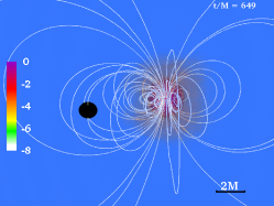
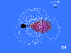
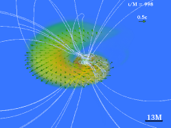
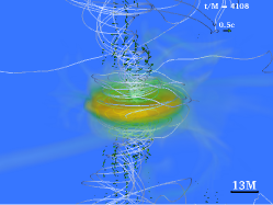
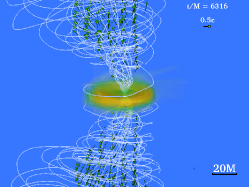
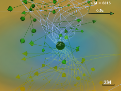
Figure 43: Evolution of the profile of the rest-mass density (normalized by its initial maximum value), the location of the apparent horizon (black filled sphere), and the magnetic-field lines (white solid) for a binary with $Q=3$, $\chi=0.75$, and $\mathcal{C}=0.145$ modeled by a $\Gamma=2$ polytrope. The maximum value of the initial magnetic-field strength is $\approx${10}^{17}\text{\,}\mathrm{G}$(1.4\,M_{\odot}/M_{\mathrm{NS}})$. Image reproduced with permission from Paschalidis et al. (2015), copyright by AAS.

If the neutron star is seeded with strong dipolar magnetic fields aligned with the orbital angular momentum of the binary at the outset, a collimated outflow with possibly ultrarelativistic terminal velocity may be launched from the remnant black hole–disk system (Paschalidis et al., 2015). Figure 43 generated by Paschalidis et al. (2015) illustrates the rest-mass density and the structure of magnetic fields for a system with $Q=3$, $\chi=0.75$, $\mathcal{C}=0.145$ modeled by a $\Gamma=2$ polytrope, and the initial dipolar magnetic field reaching up to $\approx${10}^{17}\text{\,}\mathrm{G}$(1.4\,M_{\odot}/M_{\mathrm{NS}})$ in the stellar interior. Strong magnetic fields are helpful for resolving the magnetorotational instability in the accretion disk with a sufficient number of grids, and the magnetic stress in this system is found to correspond to $\alpha_{\nu}\approx 0.01$–0.04. Although this value is broadly consistent with results obtained by numerical studies of other similar systems (see, e.g., Kiuchi et al., 2018; Fernández et al., 2019), the value of $\alpha_{\nu}$ has not yet settled due to the difficulty in achieving convergence in three-dimensional magnetohydrodynamics simulations. Actually, it is not claimed that the magnetorotational instability is resolved in Paschalidis et al. (2015).

The results of Paschalidis et al. (2015) suggest that strong poloidal magnetic fields on a large scale may be essential for driving an ultrarelativistic jet in the low-density polar region, which may become force-free in the real world. While differential rotation of the tidal tail amplifies the toroidal field after tidal disruption, the poloidal component still persists and connects distinct portions of the remnant disk. The differential rotation of the disk continues to twist the poloidal component in the polar region, and the amplified toroidal field eventually overcomes the ram pressure and establishes a funnel-like, low-density environment. A collimated and mildly-relativistic outflow is driven in this region with the Lorentz factor of $\approx 1.2$–$1.3$ (equivalently, $\sim 0.6c$) and the opening angle of $\sim$$$. However, the acceleration cannot be fully tracked to the terminal velocity, because a force-free environment cannot be resolved and, as a result, the acceleration to ultrarelativistic velocity close to the speed of light is prohibited in magnetohydrodynamics simulations. Despite this limitation, the terminal Lorentz factor in Paschalidis et al. (2015) is suggested to be as large as $\sim 100$ if the baryon loading is not severe. In addition, the large terminal Lorentz factor is realized only if the magnetic-field energy is converted efficiently to the kinetic energy of the material (see, e.g., Rees and Gunn 1974; Kennel and Coroniti 1984 for the so-called sigma problem in the pulsar wind nebula). Because the Poynting luminosity reaches ${10}^{51}\text{\,}\mathrm{e}\mathrm{r}\mathrm{g}\,\mathrm{s}^{-1}$ and the accretion time scale is estimated to be $\sim$0.5\text{\,}\mathrm{s}$$, their results support the idea that the Blandford-Znajek mechanism drives a short-hard gamma-ray burst in black hole–neutron star binaries if the assumed magnetic-field configuration is realistic.

However, all this depends on whether strong poloidal magnetic fields presumed in Paschalidis et al. (2015) at the outset are developed on a large scale within the lifetime of the accretion disk. Actually, their own follow-up study revealed that the dipolar field tilted by $90\mathrm{°}$ did not allow an outflow to be launched (Ruiz et al., 2018). This may be reasonable, because the tilt angle of $90\mathrm{°}$ eliminates net vertical magnetic fields threading the orbital plane. This finding indicates the importance of deriving the strength and geometry of magnetic fields at the disk formation in a self-consistent manner by merger simulations, even if it is a computationally challenging task (Etienne et al., 2012a, c). Although the Kelvin-Helmholtz instability at disk circularization and subsequent magnetorotational instability rapidly amplify small-scale magnetic fields (Kiuchi et al., 2015b, see also Kiuchi et al. 2015a for magnetic-field amplification at the contact surface of binary neutron stars), it is not obvious whether and, if yes, how globally coherent fields stronger than the initial fields are developed.

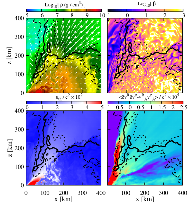
Figure 44: Profile of the rest-mass density (left top), the plasma $\beta$, i.e., the ratio of the gas pressure to the magnetic pressure, (right top), the thermal part of the specific internal energy (left bottom), and the sum of Maxwell and Reynolds stress (right bottom) on the meridional plane at $\approx$50\text{\,}\mathrm{ms}$$ after the onset of merger for a binary with $M_{\mathrm{BH}}=5.4\,M_{\odot}$, $\chi=0.75$, $M_{\mathrm{NS}}=1.35\,M_{\odot}$, and $R_{\mathrm{NS}}=$13.6\text{\,}\mathrm{km}$$ ($Q=4$, $\mathcal{C}=0.147$) modeled by a piecewise-polytropic approximation of the H4 equation of state (Glendenning and Moszkowski, 1991; Lackey et al., 2006). The maximum value of the initial magnetic-field strength is $\approx${10}^{15}\text{\,}\mathrm{G}$$. The white arrows in the left top panel denote the velocity field on this plane. The black contours indicate $u_{t}=-0.98$ (thick dashed), $-1$ (solid), and $-1.02$ (thin dashed). Image reproduced with permission from Kiuchi et al. (2015b), copyright by APS.

If a magnetohydrodynamical disk outflow is launched, global poloidal magnetic fields are likely to be developed due to the flux freezing. Actually, fully-relativistic magnetohydrodynamics simulations have witnessed the launch of a disk outflow from the innermost region of the accretion disk with high velocity as shown in Fig. 44 (Kiuchi et al., 2015b). As a result, the wind generates strong and coherent magnetic fields, which may subsequently extract rotational energy of the black hole via the Blandford-Znajek mechanism with the luminosity of ${10}^{49}$–${10}^{50}\text{\,}\mathrm{e}\mathrm{r}\mathrm{g}\,\mathrm{s}^{-1}$. To achieve this luminosity, a coherent magnetic field with $\gtrsim${10}^{14}\text{\,}\mathrm{G}$$ needs to penetrate the black hole. Although numerical convergence is not fully confirmed, the magnetorotational instability is likely to be resolved in the highest-resolution simulation with the grid spacing of $120\text{\,}\mathrm{m}$ in Kiuchi et al. (2015b).

It is worthwhile to note that Liska et al. (2020) demonstrated that poloidal magnetic fields can be generated from purely toroidal fields in very-high-resolution simulations for an accretion disk in a fixed, Kerr black-hole background. This global poloidal field is generated by a runaway growth of one of flux loops generated locally in a stochastic manner. The realistic magnetic fields and subsequent outflows may be clarified by future numerical-relativity simulations if the computational resources allow us to achieve sufficiently high resolutions.

One caveat in most magnetohydrodynamics simulations of black hole–neutron star binary coalescences performed to date is that neutrino transport is not taken into account. It is unclear whether magnetohydrodynamical disk outflows like that found in Kiuchi et al. (2015b) are driven in the presence of neutrino cooling. Actually, this outflow is not observed in neutrino-radiation magnetohydrodynamics simulations performed by Most et al. (2021b), although this difference may simply be ascribed to the insufficient grid resolution. A sufficiently-high-resolution numerical-relativity simulation of the whole coalescence process with detailed microphysics will become a milestone for clarifying realistic magnetic-field configurations, postmerger evolution, jet launch, and mass ejection. Last but not least, for clarifying the jet launch in particular, we need to develop novel numerical techniques for accurately resolving the force-free environment with low density and strong magnetic fields.

3.6 Gravitational waves

The last topic of Sect. 3 is gravitational waves from the merger of black hole–neutron star binaries. After discussing general features of the time- and frequency-domain waveforms in Sect. 3.6.1 and Sect. 3.6.2, respectively, we quantify the correlation between the hypothetical neutron-star equation of state and the cutoff frequency of the spectrum observed in the final inspiral and merger phases in Sect. 3.6.3. Our discussions are based mainly on systematic surveys performed in Kyutoku et al. (2010, 2011a), because the features of gravitational waves are qualitatively the same among the results obtained by independent groups. We also focus on the dominant $l=\absolutevalue{m}=2$ modes of gravitational waves from nonprecessing binaries, because they have been studied systematically in previous work. Higher harmonic modes and precession-induced modulation are discussed briefly in Sect. 3.6.4 while keeping in mind that further investigations are required to understand these topics in black hole–neutron star binaries. In this Sect. 3.6, we adopt geometrical units in which $G=c=1$.

We note that the remnant disk does not emit gravitational waves significantly unless instabilities such as the Papaloizou-Pringle instability set in (Papaloizou and Pringle, 1977). While it has been suggested that nearly-extremally-spinning black hole–neutron star binary coalescences may be accompanied by gravitational waves from massive remnant disks, this issue has not yet been settled (Lovelace et al., 2013). Thus, postmerger gravitational waves from black hole–neutron star binary coalescences are considered to be composed either of a ringdown signal from the remnant black hole or of a steep shutdown of the amplitude due to tidal disruption (see below). This point is in stark contrast with postmerger gravitational waves from binary-neutron-star coalescences, which can be highly diverse depending on masses and equations of state of neutron stars (see, e.g., Hotokezaka et al., 2013a).

3.6.1 Waveform

In preparation for discussing gravitational waveforms from black hole–neutron star binaries, it would be useful to review those from binary black holes, which have been detected more often than on a weekly basis in the LIGO-Virgo O3 (Abbott et al., 2019a, 2021a, see also Jani et al. 2016; Healy et al. 2019; Boyle et al. 2019 for catalogs of gravitational waveforms derived in numerical relativity). In the inspiral phase, the orbital frequency continues to increase due to gravitational radiation reaction. Both the amplitude and the frequency of gravitational waves increase accordingly, and the waveform with this feature is observed as the so-called chirp signal. As the merger approaches, general-relativistic effects on the orbital motion such as the spin-orbit and spin-spin couplings gradually become significant. While the waveform remains to be of the chirp type, an accurate description requires increasingly higher-order post-Newtonian corrections in this phase (see Blanchet 2014 for reviews). The merger time may be identified by the time at which the amplitude becomes maximum, and the waveform during the merger phase is smoothly connected with the chirp waveform in the inspiral phase and the ringdown waveform in the postmerger phase. A reliable merger waveform can be derived only by numerical-relativity simulations (see, e.g., Centrella et al. 2010; Duez and Zlochower 2019 for reviews). Gravitational waves in the postmerger phase are dominated by the ringdown waveform, which is a superposition of quasinormal modes of the remnant Kerr black holes (see, e.g., Berti et al. 2009 for reviews). It should be pointed out that gravitational waves associated with the quasinormal modes are emitted efficiently in the coalescence of binary black holes, because the merging process is highly nonaxisymmetric and dynamical.

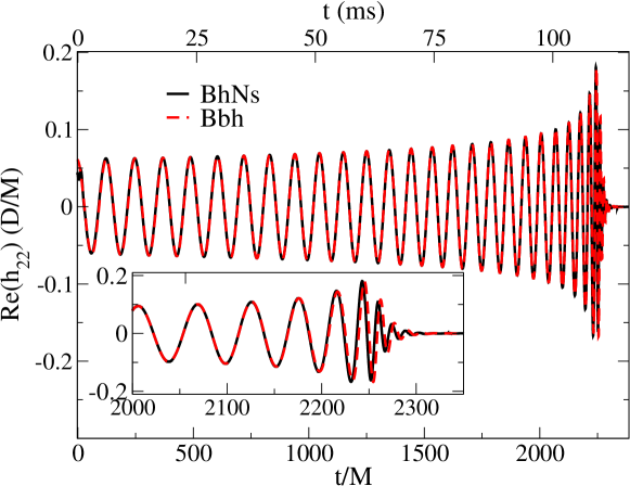
Figure 45: Comparison of the $l=\absolutevalue{m}=2$ mode of gravitational waveforms for black hole–neutron star binaries (black solid) and binary black holes (red dashed) for systems with $Q=6$, $\chi=0$, and $\mathcal{C}=0.156$ (for the black hole–neutron star binary) modeled by a $\Gamma=2$ polytrope. Image reproduced with permission from Foucart et al. (2013a), copyright by APS.

If the neutron star is not significantly deformed (and thus not disrupted) by the black hole, gravitational waveforms from black hole–neutron star binaries are essentially the same as those from binary black holes with the same values of the masses and the spins. Figure 45 generated by Foucart et al. (2013a) is a comparison of the two waveforms for systems with $Q=6$, $\chi=0$, and $\mathcal{C}=0.156$ (for the black hole–neutron star binary) derived by numerical-relativity simulations. Because tidal disruption is absent for this nonspinning black hole–neutron star binary with a high mass ratio, the two waveforms are practically indistinguishable. While a slight deviation is found during and after merger, this is within estimated numerical errors. This indistinguishability generally holds for nondisruptive systems, which are typical for high mass ratios, zero or retrograde spins of the black hole, and/or large compactnesses of the neutron star.

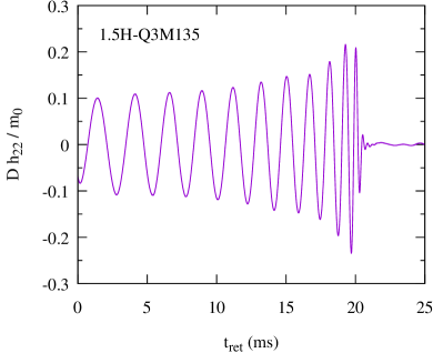
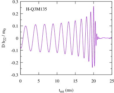
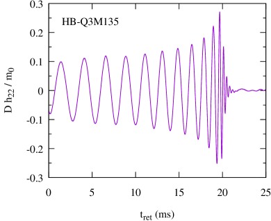
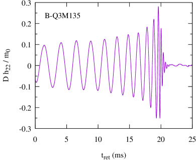
Figure 46: $l=\absolutevalue{m}=2$ mode of gravitational waveforms for black hole–neutron star binaries modeled by various equations of state. The left top, right top, left bottom, and right bottom panels show the results for a very stiff (1.5H: $R_{\mathrm{NS}}=$13.7\text{\,}\mathrm{km}$$, $\mathcal{C}=0.146$), stiff (H: $R_{\mathrm{NS}}=$12.3\text{\,}\mathrm{km}$$, $\mathcal{C}=0.162$), moderate (HB: $R_{\mathrm{NS}}=$11.6\text{\,}\mathrm{km}$$, $\mathcal{C}=0.172$), and soft (B: $R_{\mathrm{NS}}=$11.0\text{\,}\mathrm{km}$$, $\mathcal{C}=0.182$) equations of state, respectively (Read et al., 2009b; Lackey et al., 2012). Other parameters are fixed to be $M_{\mathrm{BH}}=4.05\,M_{\odot}$, $\chi=0$, and $M_{\mathrm{NS}}=1.35\,M_{\odot}$ ($Q=3$). This figure is generated from data of Kyutoku et al. (2010); Lackey et al. (2012).

Presence of the neutron-star matter influences gravitational waves from black hole–neutron star binaries for the cases in which tidal effects are strong, particularly in the merger and postmerger phases. Figure 46 displays gravitational waves from nonspinning, $\chi=0$ black hole–neutron star binaries with $M_{\mathrm{BH}}=4.05\,M_{\odot}$, $M_{\mathrm{NS}}=1.35\,M_{\odot}$ ($Q=3$) and various equations of state (Kyutoku et al., 2010). The most prominent imprint of tidal disruption is the abrupt shutdown of gravitational-wave emission and suppression of the ringdown waveform for low mass-ratio binaries with low-compactness neutron stars, e.g., for 1.5H-Q3M135 in Fig. 46. The primary mechanism for the suppression of the ringdown waveform is phase cancellation (Nakamura and Sasaki, 1981; Shapiro and Wasserman, 1982; Nakamura and Oohara, 1983). That is, quasinormal modes are excited only incoherently by the infall of widely-spread material as depicted in the left panel of Fig. 18, and thus their amplitude is reduced by the interference. This effect is enhanced more appreciably for a neutron star with a larger radius, which is disrupted at a more distant orbit from the innermost stable circular orbit. Here, it is appropriate to point out that the incoherent infall of the widely-spread material is realized because of the small radius of a low-mass black hole compared to that of a neutron star. We recall that, if the black hole is nonspinning, tidal disruption is possible only for low mass-ratio systems discussed here. If the spin parameter of the black hole is large, tidal disruption becomes possible for high mass-ratio systems, and the gravitational waveform may exhibit different features as we discuss later.

The gravitational-wave frequency at which this shutdown occurs is determined approximately by the orbital frequency at which tidal disruption occurs. One important remark is that this is in general distinct from the orbital frequency at the onset of mass shedding. Even after the mass shedding sets in, the neutron star remains to be approximately gravitationally self-bound and preserves its orbital evolution as a two-body system for a while. Tidal disruption occurs only after the orbital separation decreases further as a result of continued emission of inspiral-like gravitational waves. Because the gravitational-wave amplitude suddenly decreases only at tidal disruption, the orbital frequency at the onset of mass shedding may not leave noticeable imprints in the waveform. By contrast, if the neutron star is not disrupted, e.g., Fig. 45 and B-Q3M135 in Fig. 46, the maximum frequency is determined universally by the quasinormal mode of the remnant black hole. This is because most of the neutron-star material falls into the black hole simultaneously through a narrow region (see the middle panel of Fig. 18) and the quasinormal modes are excited efficiently. The maximum amplitude of gravitational waves also becomes as large as that of binary black holes in the absence of tidal disruption.

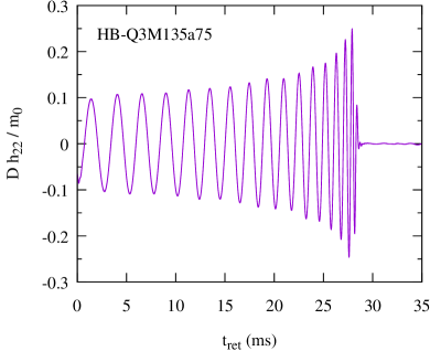
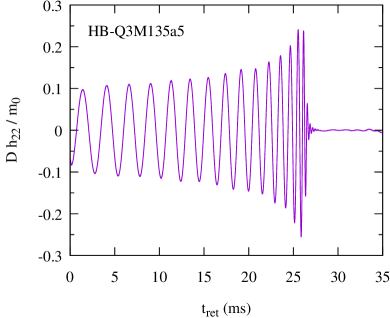
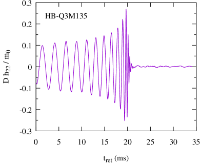
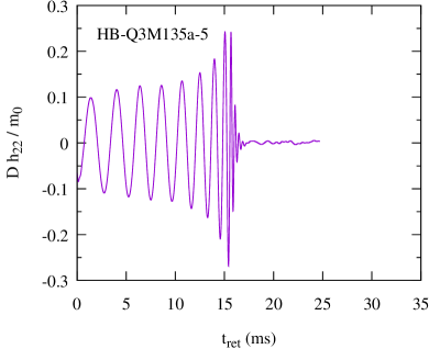
Figure 47: Same as Fig. 46 but for various values of the black-hole spin. The left top, right top, left bottom, and right bottom panels show the results for $\chi=0.75$, $0.5$, $0$, and $-0.5$, respectively. Other parameters are fixed to be $M_{\mathrm{BH}}=4.05\,M_{\odot}$, $M_{\mathrm{NS}}=1.35\,M_{\odot}$, and $R_{\mathrm{NS}}=$11.6\text{\,}\mathrm{km}$$ ($Q=3$, $\mathcal{C}=0.172$) modeled by a piecewise polytrope called HB (Read et al., 2009b). All the models have the same values of the initial orbital angular velocity, $m_{0}\Omega=0.030$. The result for HB-Q3M135 has already been shown in Fig. 46, but we replot it for comparison. This figure is generated from data of Kyutoku et al. (2010, 2011a).

The spin of the black hole also modifies the gravitational waveform qualitatively as it affects the merger process (Sect. 3.3) and properties of the remnant (Sect. 3.4). Figure 47 displays gravitational waves from black hole–neutron star binaries with $M_{\mathrm{BH}}=4.05\,M_{\odot}$, $M_{\mathrm{NS}}=1.35\,M_{\odot}$, $R_{\mathrm{NS}}=$11.6\text{\,}\mathrm{km}$$ ($Q=3$, $\mathcal{C}=0.172$) modeled by a piecewise polytrope called HB for various values of the (anti-)aligned spin of the black hole. This figure clearly shows that the lifetime of the binary and the number of gravitational-wave cycles in the inspiral phase increase as the spin of the black hole increases. This is caused mainly by the spin-orbit coupling as described in Sect. 3.3.3.

Figure 47 also illustrates that gravitational waveforms in the merger phase are modified qualitatively by the spin of the black hole, because it critically affects the final fate of the companion neutron star. In particular, the quasinormal-mode excitation is suppressed for HB-Q3M135a75 with $\chi=0.75$ compared to HB-Q3M135 with $\chi=0$. This is because the radius of the innermost stable circular orbit is decreased and tidal disruption occurs far outside it if the black hole has a prograde spin. Conversely, quasinormal modes are clearly visible for zero and retrograde spins of the black hole, $\chi\leq 0$, because tidal disruption does not occur. Remarkably, HB-Q3M135a5 with $\chi=0.5$ shows the ringdown signal, although the neutron star is tidally disrupted and leaves the material as much as $0.11\,M_{\odot}$ outside the apparent horizon at $10\text{\,}\mathrm{ms}$ after the onset of merger. The reason that the quasinormal modes are excited even if the neutron star is tidally disrupted is that the tidal disruption occurs only near the innermost stable circular orbit and thus the infall of the disrupted material proceeds from a narrow region of the black-hole surface without spreading around it (see the right panel of Fig. 18).

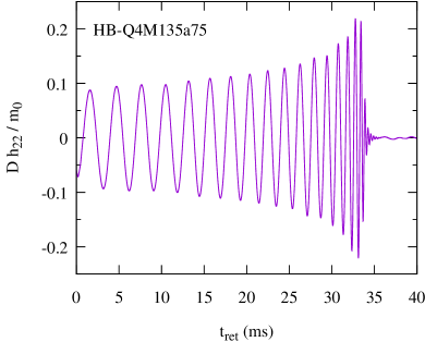
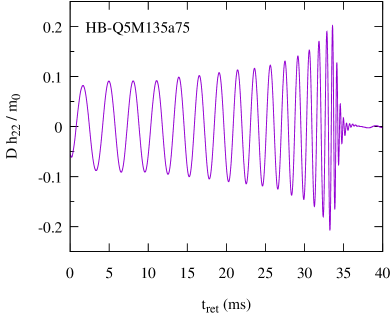
Figure 48: Same as Fig. 46 but for two values of the mass ratio. The left and right panels show the results for $M_{\mathrm{BH}}=5.4\,M_{\odot}$ ($Q=4$) and $6.75\,M_{\odot}$ ($Q=5$), respectively (see also the left top panel of Fig. 47 for $Q=3$). Other parameters are fixed to be $\chi=0.75$, $M_{\mathrm{NS}}=1.35\,M_{\odot}$, and $R_{\mathrm{NS}}=$11.6\text{\,}\mathrm{km}$$ ($\mathcal{C}=0.172$) modeled by a piecewise polytrope called HB (Read et al., 2009b). This figure is generated from data of Kyutoku et al. (2011a).

Tidal disruption of the neutron star in high mass-ratio systems is typically compatible with the quasinormal-mode excitation of the remnant black hole. Figure 48 displays the gravitational waveforms for black hole–neutron star binaries with $\chi=0.75$, $M_{\mathrm{NS}}=1.35\,M_{\odot}$, $R_{\mathrm{NS}}=$11.6\text{\,}\mathrm{km}$$ ($\mathcal{C}=0.172$) modeled by a piecewise polytrope called HB, and two different values of the black-hole mass $M_{\mathrm{BH}}=5.4\,M_{\odot}$ ($Q=4$, left) and $6.75\,M_{\odot}$ ($Q=5$, right). The ringdown waveform is clearly visible for both systems due to the same reason as that described above for HB-Q3M135a5. Although tidal disruption is less significant for higher mass-ratio systems, HB-Q5M135a75 with $Q=5$ still leaves $0.095\,M_{\odot}$ outside the apparent horizon at $10\text{\,}\mathrm{ms}$ after the onset of merger. Thus, the excitation of quasinormal modes cannot be ascribed to the absence of tidal disruption. The existence of the ringdown waveform, however, does not imply that the entire waveform is identical to that of binary black holes. We discuss this point further using the spectrum in Sect. 3.6.2.

3.6.2 Spectrum

Gravitational waves in the frequency domain clearly exhibit rich information about their sources. Frequency-domain gravitational waveforms are also useful for applications to gravitational-wave data analysis, which is usually performed in the frequency domain. For the early stage of the inspiral phase, during which the orbital frequency is $\lesssim$1\text{\,}\mathrm{kHz}$$, the spectral amplitude and phase of the frequency-domain waveform agree approximately with those derived by the post-Newtonian calculations. The effective spectral amplitude defined by $h_{\mathrm{eff}}:=f\absolutevalue*{\tilde{h}(f)}$, where $\tilde{h}(f)$ is the Fourier transform of the time-domain waveform, behaves universally as $\propto f^{-1/6}$ at low frequency in accordance with the prediction of the quadrupole formula (see, e.g., Thorne, 1987; Sathyaprakash and Dhurandhar, 1991). The gravitational-wave phase is determined primarily by the chirp mass, $\mathcal{M}:=M_{\mathrm{BH}}^{3/5}M_{\mathrm{NS}}^{3/5}/m_{0}^{1/5}$, and thus $\mathcal{M}$ is determined with high accuracy by analyzing gravitational waves in this stage (Sathyaprakash and Dhurandhar, 1991; Finn and Chernoff, 1993). In closer inspiral orbits with higher frequency, the spectral index increases as the nonlinearity of general relativity and finite-size effects of the neutron star become important at the small orbital separation. In this stage, we may be able to extract the mass ratio, which allows us to determine the masses of individual components, and spin parameters of the binary (Cutler and Flanagan, 1994; Poisson and Will, 1995). These measurements are indeed realized for black hole–neutron star binaries in LIGO-Virgo O3 (Abbott et al., 2021a, b). Tidal deformability of the neutron star may also be extracted if the finite-size effect is appreciable and the signal-to-noise ratio is large (Flanagan and Hinderer, 2008).

The final fate of the neutron star in black hole–neutron star binaries is clearly reflected in the damping of the gravitational-wave spectrum at high frequency of $f\gtrsim$1\text{\,}\mathrm{kHz}$$. If tidal disruption (not the mass shedding) occurs at a distant orbit from the innermost stable circular orbit, the spectral amplitude of gravitational waves is characterized by damping above cutoff frequency, $f_{\mathrm{cut}}$. Its precise value is given by the frequency of gravitational waves in the last stage of the inspiral phase, $\sim 1$–$2\text{\,}\mathrm{kHz}$, and depends primarily on the compactness of the neutron star (see Sect. 1.3.1). If tidal deformation (and thus disruption) is not significant, the spectrum in the high-frequency range agrees approximately with that for binary black holes. Even if the neutron star is tidally disrupted near the innermost stable circular orbit, the inspiral-like motion continues inside it on a dynamical time scale and gravitational waves with a large amplitude are emitted. Thus, the effective amplitude, $h_{\mathrm{eff}}(f)$, is larger than the case in which tidal effects play a significant role in determining the final fate of the binary coalescence. If the tidal effect is very weak, the effective amplitude even increases for $f\gtrsim$1\text{\,}\mathrm{kHz}$$ until it damps exponentially above the cutoff frequency determined by quasinormal modes of the remnant black hole in a similar manner to the case of binary-black-hole coalescences. A proposal for quantitative definition of the cutoff frequency will be reviewed later in Sect. 3.6.3.

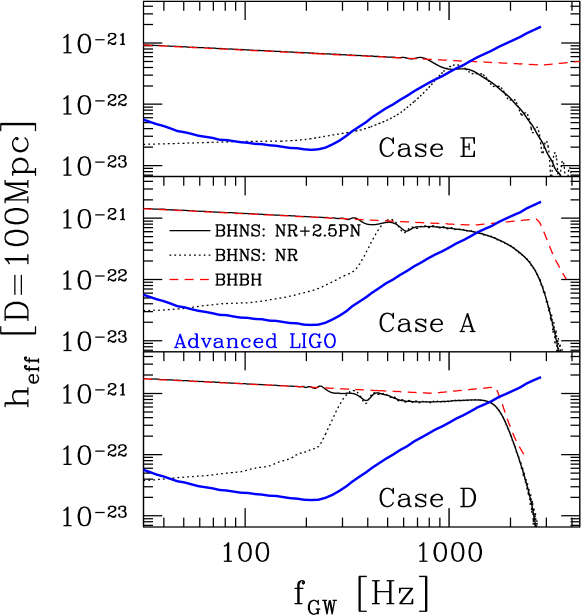
Figure 49: Gravitational-wave spectrum for black hole–neutron star binaries with $Q=1$ (top: Case E), $3$ (middle: Case A), and $5$ (bottom: Case D). Other parameters are fixed to be $\chi=0$ and $\mathcal{C}=0.145$ modeled by a $\Gamma=2$ polytrope. To plot the curves in physical units, the baryon rest mass of the neutron star is set to be $1.4\,M_{\odot}$ and the distance of $D=$100\text{\,}\mathrm{M}\mathrm{p}\mathrm{c}$$ is assumed. The black solid curves show the spectra of hybrid waveforms constructed by a second-and-a-half-order post-Newtonian approximation and numerical-relativity simulations, while the black dotted curves show only the latter. The red dashed curve shows the so-called PhenomA model for binary black holes (Ajith et al., 2008). The blue solid curve is the noise spectral density of the Advanced LIGO planned as of 2009. Image reproduced with permission from Etienne et al. (2009).

Figure 49 generated by Etienne et al. (2009) displays the variation of the spectral cutoff with respect to the degree of tidal disruption by comparing results for nonspinning black hole–neutron star binaries with different mass ratios (equivalently, different masses of the black holes with the same mass and radius of the neutron stars). The top panel for $Q=1$ shows that the spectrum damps at $f\sim$1\text{\,}\mathrm{kHz}$$, which is far below the quasinormal-mode frequency for the remnant black hole of $\sim$6\text{\,}\mathrm{kHz}$$. The cutoff of this spectrum reflects tidal disruption at a distant orbit from the innermost stable circular orbit. The bottom panel for $Q=5$ shows that the cutoff frequency of this spectrum agrees approximately with the quasinormal-mode frequency, because tidal disruption is insignificant. The middle panel for $Q=3$ shows intermediate behavior. Specifically, the cutoff frequency is determined by tidal disruption which occurs near the innermost stable circular orbit.

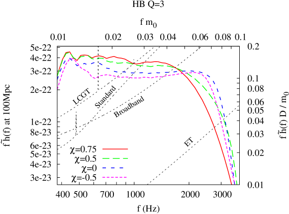
Figure 50: Gravitational-wave spectrum of the $l=\absolutevalue{m}=2$ mode for black hole–neutron star binaries with various values of the black-hole spin. Other parameters are fixed to be $M_{\mathrm{BH}}=4.05\,M_{\odot}$, $M_{\mathrm{NS}}=1.35\,M_{\odot}$, and $R_{\mathrm{NS}}=$11.6\text{\,}\mathrm{km}$$ ($Q=3$, $\mathcal{C}=0.172$) modeled by a piecewise polytrope called HB (Read et al., 2009b). These spectra are derived from the waveforms shown in Fig. 47, and the cutoff at $f\lesssim$400\text{\,}\mathrm{Hz}$$ results from the fact that numerical simulations started there. The left and bottom axes show these quantities in physical units assuming that the observer is located at $100\text{\,}\mathrm{M}\mathrm{p}\mathrm{c}$ along the direction perpendicular to the orbital plane. The right and top axes show normalized, dimensionless amplitude and frequency, respectively. The dashed curves labeled by “Standard” and “Broadband” are two options for the noise spectral density of the Advanced LIGO planned as of 2011. Those labeled by “LCGT” and “ET” are the planned noise spectral density of KAGRA, formerly called LCGT, and the Einstein Telescope, respectively. Image adapted from Kyutoku et al. (2011a); copyright by APS.

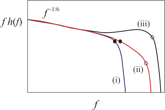
Figure 51: Schematic description of three types of gravitational-wave spectra for black hole–neutron star binaries. The filled and open circles denote frequency associated with tidal disruption and a quasinormal mode of the remnant black hole, respectively. The spectrum (i) corresponds to the case depicted in the left panel of Fig. 18, for which tidal disruption is induced by a black hole with a small mass. The spectrum (ii) corresponds to the case depicted in the middle panel of Fig. 18, for which tidal disruption is induced by a black hole with a large mass and a high spin. The spectrum (iii) corresponds to the case depicted in the right panel of Fig. 18, for which tidal disruption does not occur as the black hole is massive and does not have a high prograde spin.

The spin of the black hole is the key for observing cutoff behavior associated with tidal disruption (Etienne et al., 2009; Kyutoku et al., 2011a). Figure 50 shows that the spectrum depends quantitatively and also qualitatively on the black-hole spin. Because tidal disruption does not occur significantly for systems with $\chi\leq 0$ shown in this figure, the cutoff frequency, $f_{\mathrm{cut}}$, is $\sim 2.5$–$3\text{\,}\mathrm{kHz}$ determined by the quasinormal modes of the remnant black holes with $\sim 5.3\,M_{\odot}$. For the system with $\chi=0.75$, the cutoff frequency becomes as low as $f_{\mathrm{cut}}\sim 1.5$–$2\text{\,}\mathrm{kHz}$, because tidal disruption occurs outside the innermost stable circular orbit. Notably, the system with $\chi=0.5$ shows both of these features. That is, the spectrum for $\chi=0.5$ first exhibits softening of the spectrum at $f\sim$2\text{\,}\mathrm{kHz}$$ associated with tidal disruption and next damps exponentially above $f\sim$3\text{\,}\mathrm{kHz}$$ associated with the quasinormal mode, consistently with the gravitational waveform of HB-Q3M135a5 (exactly the same model) shown in the left top panel of Fig. 47. Hereafter, we refer to the former as the cutoff frequency, because we are primarily interested in tidal disruption. This type of the spectrum is produced for the case depicted in the right panel of Fig. 18, and schematic gravitational-wave spectra for these three types of the merger process are shown in Fig. 51.

The spin-orbit coupling described in Sect. 3.3.3 induces two features preferable for observing the cutoff frequency by gravitational-wave detectors if the spin is prograde. First, because the prograde spin reduces the orbital angular velocity to maintain a circular orbit for a given orbital separation, the cutoff frequency of gravitational waves at tidal disruption is reduced. Next, the effective amplitude before tidal disruption increases for given frequency due to the reason explained by the following post-Newtonian argument (Kyutoku et al., 2011a). By retaining only the first-and-a-half-order post-Newtonian term related to the spin-orbit coupling, the binding energy of the system, $E$, as a function of the gravitational-wave frequency behaves as (Kidder, 1995)

$$\derivative{E}{f}=\frac{Q}{3(1+Q)^{2}}\frac{(\pi m_{0}f)^{5/3}}{\pi f^{2}}\bqty{1+\chi\hat{\mathbf{S}}\dotproduct\hat{\mathbf{L}}\frac{5(4Q+3)}{3(1+Q)^{2}}(\pi m_{0}f)},$$ (45)

where $\hat{\mathbf{S}}$ and $\hat{\mathbf{L}}$ are the unit vectors in the direction of the black-hole spin and the orbital angular momentum, respectively. Note that we have also neglected the spin of the neutron star. Here, $\derivative*{E}{f}$ is related to the effective amplitude via

$$\derivative{E}{f}\propto\bqty{f\absolutevalue{\tilde{h}(f)}}^{2}=h_{\mathrm{eff}}^{2}(f).$$ (46)

Thus, for given frequency, the effective amplitude increases as the spin of the black hole increases in the prograde direction, reflecting the fact that the binary has to emit larger energy via gravitational waves for increasing the orbital angular velocity against the spin-orbit repulsive force. These two effects are clearly shown in Fig. 50.

Arguably the most important feature of the cutoff frequency is that it depends on the equation of state of the neutron star, in particular the average density (see Sect. 1.3.1). Thus, the cutoff frequency will give us information about the equation of state for supranuclear-density matter, particularly if it is stiff (Vallisneri, 2000).

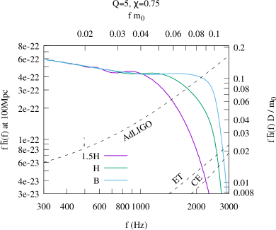
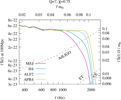
Figure 52: Same as Fig. 50 but for binaries with $\chi=0.75$ and $M_{\mathrm{NS}}=1.35\,M_{\odot}$ modeled by various equations of state. The left panel is for $M_{\mathrm{BH}}=6.75\,M_{\odot}$ ($Q=5$), and the equations of state are taken to be piecewise polytropes called 1.5H ($R_{\mathrm{NS}}=$13.7\text{\,}\mathrm{km}$$, $\mathcal{C}=0.146$), H ($R_{\mathrm{NS}}=$12.3\text{\,}\mathrm{km}$$, $\mathcal{C}=0.162$), and B ($R_{\mathrm{NS}}=$11.0\text{\,}\mathrm{km}$$, $\mathcal{C}=0.182$) (Read et al., 2009b; Lackey et al., 2012). The right panel is for $M_{\mathrm{BH}}=9.45\,M_{\odot}$ ($Q=7$), and the equations of state are taken to be piecewise polytropic approximations of MS1 (Müller and Serot, 1996, $R_{\mathrm{NS}}=$14.4\text{\,}\mathrm{km}$$, $\mathcal{C}=0.138$), H4 (Glendenning and Moszkowski, 1991; Lackey et al., 2006, $R_{\mathrm{NS}}=$13.6\text{\,}\mathrm{km}$$, $\mathcal{C}=0.147$), ALF2 (Alford et al., 2005, $R_{\mathrm{NS}}=$12.4\text{\,}\mathrm{km}$$, $\mathcal{C}=0.161$), and APR4 (Akmal et al., 1998, $R_{\mathrm{NS}}=$11.1\text{\,}\mathrm{km}$$, $\mathcal{C}=0.180$). The dashed curves labeled by “AdLIGO,” “ET,” and “CE” are the noise spectral density of the Advanced LIGO at the design sensitivity, Einstein Telescope, and Cosmic Explorer, respectively, taken from Abbott et al. (2017a). The left and right panels are generated from data of unpublished work and Kyutoku et al. (2015), respectively.

Figure 52 plots the gravitational-wave spectrum for black hole–neutron star binaries with $\chi=0.75$ and $M_{\mathrm{NS}}=1.35\,M_{\odot}$ modeled by a variety of equations of state. In this figure, $M_{\mathrm{BH}}$ is taken to be $6.75\,M_{\odot}$ (left: $Q=5$, unpublished) and $9.45\,M_{\odot}$ (right: $Q=7$, Kyutoku et al., 2015). This figure clearly shows that the cutoff frequency at which the effective amplitude begins to damp depends on the equation of state for given values of the mass and the spin of the components. Specifically, the cutoff frequency is in the range of $\sim 1$–$2.5\text{\,}\mathrm{kHz}$ and becomes lower as the equation of state becomes stiffer (i.e., the compactness of the neutron star becomes smaller) for the systems considered here, because tidal disruption occurs at a more distant orbit with lower frequency. At the same time, the effective amplitude for given frequency at $f\gtrsim$1\text{\,}\mathrm{kHz}$$ increases as the equation of state becomes soft (i.e., the compactness becomes large). For a softer equation of state, the cutoff frequency becomes higher and saturates approximately to the quasinormal-mode frequency as tidal disruption becomes insignificant. These features are discussed in more detail in Sect. 3.6.3.

A remarkable feature of high mass-ratio systems with the high prograde spin of the black hole is that the neutron star can be tidally disrupted outside the innermost stable circular orbit for a wide range of equations of state. This feature can make variation of the spectra and the cutoff frequency visible in the sensitivity band of current ground-based detectors such as the Advanced LIGO. Thus, binaries of a high-mass, high-spin black hole and a neutron star is a promising target for studying the equation of state via the cutoff frequency. For even larger values of the black-hole spin parameter, say $\chi\geq 0.9$, tidal disruption of a neutron star with the typical mass in our Galaxy of $1.3$–$1.4\,M_{\odot}$ will also be possible for even larger values of the mass ratio, $Q\gtrsim 10$ or equivalently more massive black holes with $M_{\mathrm{BH}}\gtrsim 13$–$14\,M_{\odot}$. Exploration of tidal disruption at such a high mass-ratio regime is an important topic for a future study in numerical relativity.

Conversely, the cutoff frequency is higher than $\sim$2\text{\,}\mathrm{kHz}$$ if the mass ratio of the system is $Q\lesssim 3$. We recall that the cutoff frequency is determined not by mass shedding but by tidal disruption, which occurs in a closer orbit with higher frequency, in particular for the small values of $Q$. Thus, the cutoff frequency of low mass-ratio systems allows us to investigate neutron-star equations of state only if we are capable of detecting signals at $f\gtrsim$2\text{\,}\mathrm{kHz}$$, for which the sensitivity of detectors is degraded. Moreover, the amplitude is not very large because of the small mass. These facts imply that the study of the cutoff frequency with nonspinning black hole–neutron star binaries will await third-generation detectors such as the Einstein Telescope (Maggiore et al., 2020) and the Cosmic Explorer (Abbott et al., 2017a).

Before concluding Sect. 3.6.2, we comment on the current status of the development of phenomenological frequency-domain waveform templates with various methods utilizing results of numerical relativity. Preliminary models, one of which is called LEA, were constructed with the aid of a phenomenological model called PhenomC (Santamaría et al., 2010) or the effective-one-body formalism (Taracchini et al., 2012) by calibrating free parameters for both the amplitude and the phase with numerical-relativity simulations of black hole–neutron star binaries (Lackey et al., 2014). One of the up-to-date models, PhenomNSBH (Thompson et al., 2020), is constructed by combining an amplitude model calibrated with numerical-relativity simulations of black hole–neutron star binaries (Pannarale et al., 2015a) with a phase model consisting of a model called PhenomD for the point-particle baseline (Khan et al., 2016) and the NRTidal model for the tidal effect (Dietrich et al., 2017a, 2019), which is derived also in a phenomenological manner by calibrating free parameters with numerical-relativity simulations of binary neutron stars. Another model, SEOBNR_NSBH (Matas et al., 2020), is constructed in a similar manner except that the point-particle baseline is taken to be an effective-one-body model called SEOBNR (Bohé et al., 2017) and new numerical-relativity waveform models are used to recalibrate the amplitude model. These phenomenological models are available in LSC Algorithm Library. A common drawback among these waveform models may be that no higher harmonic mode or no precession has been modeled despite their relevance for black hole–neutron star binaries. These issues are discussed in Sect. 3.6.4. In addition, the ringdown phase is not incorporated appropriately in the phase model.

3.6.3 Correlation of the cutoff frequency and the compactness

To quantify the cutoff frequency and contained information, Shibata et al. 2009; Kyutoku et al. 2010, 2011a have fitted the gravitational-wave spectra by a function of the form

$$\frac{f\tilde{h}_{\mathrm{fit}}(f)D}{m_{0}}=\frac{f\tilde{h}_{\mathrm{3PN}}(f)D}{m_{0}}e^{-(f/f_{\mathrm{ins}})^{\sigma_{\mathrm{ins}}}}+Ae^{-(f/f_{\mathrm{dam}})^{\sigma_{\mathrm{dam}}}}\bqty{1-e^{-(f/f_{\mathrm{ins2}})^{\sigma_{\mathrm{ins2}}}}},$$ (47)

where $\tilde{h}_{\mathrm{3PN}}$ is obtained by Fourier-transforming the so-called TaylorT4 approximant (Buonanno et al., 2003), which is one variant of post-Newtonian approximants (Damour et al., 2001; Buonanno et al., 2009), and $f_{\mathrm{ins}}$, $f_{\mathrm{ins2}}$, $f_{\mathrm{dam}}$, $\sigma_{\mathrm{ins}}$, $\sigma_{\mathrm{ins2}}$, $\sigma_{\mathrm{dam}}$, and $A$ are free parameters to be determined. Then, Kyutoku et al. (2011a) determined the cutoff frequency $f_{\mathrm{cut}}$ by the higher of two frequency at which the second term of this function becomes a half of the maximum value. Note that earlier work have simply defined $f_{\mathrm{cut}}$ by $f_{\mathrm{dam}}$ (Shibata et al., 2009; Kyutoku et al., 2010), but this definition turned out to be not useful for spinning black hole–neutron star binaries, primarily because the functional form is not flexible enough to model the spectrum (ii) in Fig. 51. Robust and useful definition of the cutoff frequency, $f_{\mathrm{cut}}$, is still to be explored.

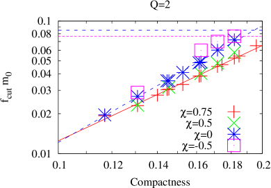
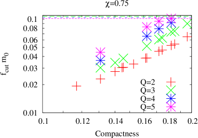
Figure 53: Relation between the normalized, dimensionless cutoff frequency $f_{\mathrm{cut}}m_{0}$ and the compactness of the neutron star $\mathcal{C}$ derived by a suite of simulations with piecewise polytropes. The left panel show the results for $Q=2$ with $\chi=0.75$, $0.5$, $0$, and $-0.5$. The red solid and blue dashed lines are results of linear fittings for $\chi=0.75$ ($f_{\mathrm{cut}}m_{0}\propto\mathcal{C}^{2.39}$) and $\chi=0$ ($f_{\mathrm{cut}}m_{0}\propto\mathcal{C}^{2.92}$), respectively. Notice that the power-law indices are larger than $3/2$ [cf., Eq. (12)]. The right panel shows the results for $\chi=0.75$ with $Q=2$, $3$, $4$, and $5$. The dashed horizontal lines in the upper parts of the plots denote typical values of the quasinormal-mode frequency for each binary parameter. Image adapted from Kyutoku et al. (2011a), copyright by APS.

Figure 53 plots the dimensionless cutoff frequency $f_{\mathrm{cut}}m_{0}$ for various systems. The left panel is for $Q=2$ with various values of $\chi$, and the right panel is for $\chi=0.75$ with various values of $Q$. This figure shows that the cutoff frequency normalized by the inverse of the total mass has a tight correlation with the compactness of the neutron star for given values of the mass ratio and the spin parameter of the black hole. Thus, if we are able to determine masses and spin parameters from gravitational-wave data analysis (see, e.g., Cutler and Flanagan, 1994; Hannam et al., 2013, for degeneracy of the mass and the spin), the cutoff frequency may enable us to constrain the compactness of the neutron star and hence the equation of state. Although it is not clear from this figure, for the case in which tidal disruption does not occur significantly, which is typical for a large compactness, the cutoff frequency settles approximately to the quasinormal-mode frequency shown in the upper part of the panels (Shibata et al., 2009; Kyutoku et al., 2010). It has also been found that, by adopting piecewise polytropes with different values of the adiabatic index for the core region, the cutoff frequency also depends weakly on the density profile of the neutron star (Kyutoku et al., 2010). This trend is consistent with that for the mass of the material remaining outside the apparent horizon described in Sect. 3.4.2.

An important finding is that the dimensionless cutoff frequency, $f_{\mathrm{cut}}m_{0}$, depends more strongly on the neutron-star compactness than expected from the mass-shedding condition, Eq. (11). Specifically, although the mass-shedding condition suggests $f_{\mathrm{cut}}m_{0}\propto\mathcal{C}^{3/2}$, the results of nonspinning black hole–neutron star binaries with $Q=2$ are found to be approximated by (Kyutoku et al., 2011a)

$$\ln(f_{\mathrm{cut}}m_{0})=(2.92\pm 0.06)\ln\mathcal{C}+(2.32\pm 0.12)$$ (48)

up to the compactness above which tidal disruption becomes insignificant. That is, $f_{\mathrm{cut}}m_{0}$ is approximately proportional to $\mathcal{C}^{3}$. It should be cautioned that this power-law index depends on the definition of $f_{\mathrm{cut}}$ (e.g., Kyutoku et al. 2010 derived a larger value of $\approx 4$) and also decreases for a prograde spin as shown in Fig. 53, specifically $f_{\mathrm{cut}}m_{0}\propto\mathcal{C}^{2.4}$ for $Q=2$ and $\chi=0.75$. Still, the index is universally larger than $3/2$ derived by the mass-shedding condition. This fact illustrates that the cutoff frequency is not determined simply by mass shedding. Actually, the steep dependence is reasonably expected, because the survival time of a neutron star against tidal disruption after the onset of mass shedding is generally longer for a more compact neutron star with a more centrally-condensed density profile.

3.6.4 Higher harmonic mode and spin-induced precession

Up to here, we have discussed only the dominant $l=\absolutevalue{m}=2$ modes of gravitational waves. They approximately represent gravitational waves observed from the direction perpendicular to the orbital plane of nonprecessing binaries. If we observe nonprecessing binaries from inclined directions, various harmonic modes contribute significantly to the observed signal, particularly because black hole–neutron star binaries are highly asymmetric in terms of the masses of components and emit odd modes such as $l=\absolutevalue{m}=3$ efficiently (Abbott et al., 2021a, b). The mode mixing induces modulation of gravitational-wave amplitude and phase, which cannot be mimicked only by the dominant mode (Foucart et al., 2021). Thus, accurate modeling of gravitational waves particularly in the strong-field regime requires us to take into account higher harmonic modes. It should also be mentioned that numerical-relativity simulations of compact binary coalescences have only recently begun to extract $m=0$ modes relevant to gravitational-wave memory in a reliable and accurate manner (Mitman et al., 2020).

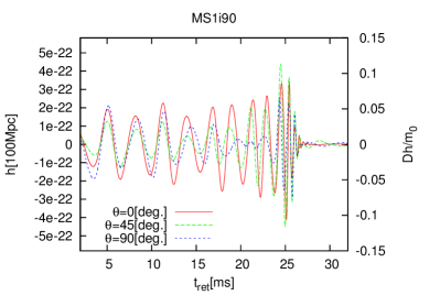
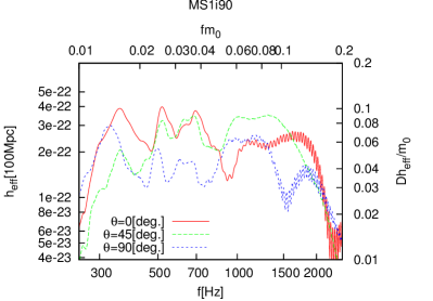
Figure 54: Plus-mode gravitational waveform (left) and spectrum (right) for a binary with $M_{\mathrm{BH}}=6.75\,M_{\odot}$, $\chi=0.75$, $M_{\mathrm{NS}}=1.35\,M_{\odot}$, and $R_{\mathrm{NS}}=$14.4\text{\,}\mathrm{km}$$ ($Q=5$, $\mathcal{C}=0.138$) modeled by a piecewise-polytropic approximation of the MS1 equation of state (Müller and Serot, 1996) observed from different directions with respect to the total angular momentum at the initial instant of simulations. All the modes with $l=2,3,$ and $4$ are included. In the left panel, the left axis shows the amplitude in physical units assuming the distance between the source and the observer to be $D=$100\text{\,}\mathrm{M}\mathrm{p}\mathrm{c}$$, and the right axis shows the dimensionless, normalized amplitude. In the right panel, the left and bottom axes show the effective amplitude and the frequency in physical units, respectively, and the right and top axes show those in the dimensionless form. The cutoff of the spectrum at $f\lesssim$300\text{\,}\mathrm{Hz}$$ results from the fact that numerical simulations started there. Image reproduced with permission from Kawaguchi et al. (2015), copyright by APS.

If the spin of the black hole is inclined with respect to the orbital angular momentum, the orbital plane precesses as shown in Fig. 19, and the amplitude and phase of gravitational waveforms are modulated due to the coupling of orbital and precessional frequency (Foucart et al., 2011, 2013b; Kawaguchi et al., 2015; Foucart et al., 2021). The left panel of Fig. 54 displays the plus-mode gravitational waveforms observed from various directions for a system with $M_{\mathrm{BH}}=6.75\,M_{\odot}$, $\chi=0.75$, $\iota\approx$$$, $M_{\mathrm{NS}}=1.35\,M_{\odot}$, and $R_{\mathrm{NS}}=$14.4\text{\,}\mathrm{km}$$ ($Q=5$, $\mathcal{C}=0.138$) modeled by a piecewise-polytropic approximation of the MS1 equation of state. In this figure, the viewing angle, $\theta$, is measured from the direction of the total angular momentum at the initial instant of the numerical simulations. Even if we observe the binary from $\theta=0$, the amplitude and phase of the waveform are modulated by the precession of the orbital plane. The modulation of the amplitude becomes stronger as the viewing angle becomes larger, because higher harmonic modes contribute more significantly to the waveform.

Mode couplings and modulation make the extraction of cutoff frequency, $f_{\mathrm{cut}}$, from the spectrum challenging in realistic observations. The right panel of Fig. 54 shows that the spectra, including their dampings for $f\gtrsim$2\text{\,}\mathrm{kHz}$$, depend significantly on the viewing angle. Because the mass ratio of this system is as high as $5$ and also tidal disruption is not very significant with leaving only $\approx 0.02\,M_{\odot}$ outside the apparent horizon due to the large inclination angle of $\approx$$$, the spectrum is expected to damp around the quasinormal-mode frequency of $\sim$2\text{\,}\mathrm{kHz}$$. However, the different amount of mode mixings prohibits straightforward extraction of the cutoff frequency independent of the viewing angle. It is a topic for future investigations how to identify the cutoff frequency which is tightly correlated with properties of neutron stars in actual observations (see Kawaguchi et al. 2017 for a preliminary study). Fortunately, the impact of higher harmonic modes on estimation of parameters common to binary black holes such as the mass and spin is likely to be marginal for black hole–neutron star binaries with moderate signal-to-noise ratios of $\lesssim 20$ (O’Shaughnessy et al., 2014a, b).

3.7 Summary and issues for the future

In this section, we have reviewed the current status of the studies on dynamical simulations of black hole–neutron star binary coalescences in full general relativity. Black hole–neutron star binaries are studied focusing mainly on their potentiality as a source of gravitational waves, a central engine of short-hard gamma-ray bursts, a site of r-process nucleosynthesis, and a progenitor of resulting kilonovae/macronovae. In the last decade, not only the parameter space surveyed has been expanded, but also qualitatively new directions have been opened by the improvement in numerical techniques and implementations. It has become popular to perform neutrino-radiation-hydrodynamics simulations with temperature- and composition-dependent equations of state. Magnetohydrodynamics simulations have also been performed frequently, although the grid resolution is still not high enough to derive robust conclusions starting from realistic profiles of the magnetic fields. In addition, qualitatively new directions of research, namely mass ejection, have been explored in numerical relativity. This direction is benefited from the development of fully-relativistic viscous hydrodynamics simulations in axisymmetry.

The final fate of the black hole-neutron star binaries is classified into two categories. One is tidal disruption of the neutron star before the plunge, and the other is the plunge of the neutron star into the black hole before tidal disruption. Tidal disruption is a more likely outcome for systems with a lower mass ratio, a higher prograde spin of the black hole, and/or a smaller compactness of the neutron star. If the black hole is nonspinning, tidal disruption of a neutron star with $\sim 1.35\,M_{\odot}$ is possible only for a low mass-ratio system with $Q\lesssim 3$ if the compactness is in a plausibly realistic range of $0.14\lesssim\mathcal{C}\lesssim 0.20$ (cf., Fig. 28). If the black hole has a high and prograde spin, tidal disruption becomes possible for a higher mass-ratio system with $Q\gtrsim 5$ because of the reduced radius of the innermost stable circular orbit.

If tidal disruption occurs sufficiently outside the innermost stable circular orbit, an accretion disk is formed and a fraction of material is ejected dynamically. The masses of the disk and the ejecta depend on the degree of tidal disruption. If the black hole is nonspinning, the mass of the remnant disk is limited to $\lesssim 0.1\,M_{\odot}$ even for a very low mass ratio. By contrast, if the spin is nearly extremal, the mass of the disk could increase to $\gtrsim 0.5\,M_{\odot}$. The mass of the dynamical ejecta is more sensitive to the mass ratio of the binary than that of the disk. For very low mass-ratio systems with $Q\lesssim 2$, the mass of the dynamical ejecta is limited to $\lesssim${10}^{-3}$\,M_{\odot}$ even if the disk as massive as $0.1\,M_{\odot}$ is formed. For high mass-ratio systems, the mass of the dynamical ejecta may become comparable to the mass of the remnant disk and could increase to $\gtrsim 0.2\,M_{\odot}$. Because the dynamical mass ejection in black hole–neutron star binaries is accompanied by neither significant shock heating nor neutrino irradiation, the dynamical ejecta preserve an extremely low electron fraction of the original neutron-star matter, $Y_{\mathrm{e}}\sim 0.05$–$0.1$. Thus, the dynamical ejecta mainly produce heavy r-process elements with the mass number $\gtrsim 130$, i.e., beyond the second peak.

The remnant disk ejects 15%–30% of its mass via viscous and/or magnetohydrodynamical processes for a wide range of physical conditions. In the early stage of the postmerger evolution, the internal energy generated by viscous or magnetohydrodynamical heating is consumed by neutrino cooling with the peak luminosity of $\gtrsim${10}^{53}\text{\,}\mathrm{e}\mathrm{r}\mathrm{g}\,\mathrm{s}^{-1}$$. At $\sim 0.1$–$1\text{\,}\mathrm{s}$ after the disk formation, the time scale of weak interactions becomes longer than the heating time scale due to the disk expansion. Because of this transition, the material in the outer part of the disk is gradually ejected in an approximately isotropic manner. The disk outflow is likely to dominate the dynamical ejecta in terms of the mass for low mass-ratio systems with $Q\lesssim 3$, while the dynamical ejecta become important for high mass-ratio systems with $Q\gtrsim 5$.

The electron fraction of the disk outflow is still uncertain. If the launch is delayed until $\gtrsim$0.5\text{\,}\mathrm{s}$$ after the disk formation, the disk outflow is characterized by an increased electron fraction of $\expectationvalue{Y_{\mathrm{e}}}\approx 0.3$ for typical cases, because the disk relaxes to an equilibrium of electron/positron captures onto nucleons during its longterm viscous or magnetohydrodynamical evolution. Neutrino irradiation also plays a role in increasing the electron fraction of the disk material in its early evolution stage of $\lesssim$0.1\text{\,}\mathrm{s}$$ as the electron antineutrinos are always the brightest. Thus, for the cases with late mass ejection, the disk outflow mainly produces light r-process elements with the mass number $80$–$130$ around the first peak. However, if the outflow is launched earlier by some mechanisms, e.g., magnetohydrodynamical activity, the electron fraction of the disk outflow could be lower. If strong and coherent poloidal magnetic fields penetrating the remnant black hole are developed as a result of binary coalescence, the merger remnant may even launch an ultrarelativistic jet via the Blandford-Znajek mechanism. However, this possibility has not been deeply explored in numerical relativity.

The final fate of the black hole–neutron star binaries is reflected in gravitational waveforms in the final inspiral and merger phases. In particular, whether tidal disruption occurs or not has a significant impact on the cutoff frequency, $f_{\mathrm{cut}}$, above which the gravitational-wave spectrum damps. If tidal disruption does not occur, quasinormal modes of the remnant black hole are excited and determine the cutoff frequency. If tidal disruption occurs around a low-mass black hole whose areal radius is comparable to or smaller than the neutron-star radius, tidal disruption suddenly suppresses gravitational-wave emission. Accordingly, the spectrum damps at the cutoff frequency corresponding to the orbital frequency at which tidal disruption occurs—not the onset of mass shedding. If tidal disruption occurs around a high-mass black hole, which has to be spinning in a prograde direction, tidal disruption does not prevent excitation of quasinormal modes. In this case, the spectrum exhibits two characteristic frequencies, one for tidal disruption and the other for quasinormal modes. These three types of merger processes and gravitational-wave spectra are presented schematically in Fig. 18 and Fig. 51, respectively.

Despite the remarkable progress made in the last decade, there still remain various issues to be explored. One important issue is to investigate tidal disruption in high mass-ratio binaries with $Q\gtrsim 10$ and/or nearly-extremally spinning black holes of $\chi\gtrsim 0.99$. Although the spin parameter of the black hole has been limited to $\chi\leq 0.97$ in the previous study of black hole–neutron star binaries, a larger value of the spin parameter can be handled in numerical relativity (Lovelace et al., 2008; Liu et al., 2009; Ruchlin et al., 2017), and simulations of binary black holes with $\chi>0.97$ have been performed (Lovelace et al., 2012; Scheel et al., 2015). Regarding the inspiral phase, systematic derivations of longterm gravitational waveforms, particularly for precessing black-hole spins (see Foucart et al. 2019a, 2021 for effort in this direction), are required to develop accurate theoretical templates toward the era of third-generation detectors. Dependence of the cutoff frequency in the gravitational-wave spectrum on neutron-star properties should be revealed thoroughly with adopting a variety of equations of state, along with developing methods for the extraction from observed gravitational-wave data. Another topic for future study in the inspiral phase is the time evolution of neutron-star magnetospheres. Because it is extremely difficult to evolve force-free magnetospheres directly by equations of the usual magnetohydrodynamics, this topic likely requires a novel method. Such simulations are also necessary for deriving realistic magnetic-field configurations at the formation of the remnant accretion disk and tracking acceleration to ultrarelativistic velocity of a possible jet. Neutrino-radiation-magnetohydrodynamics simulations in numerical relativity for the evolution of the postmerger system with the duration of $\gtrsim$1\text{\,}\mathrm{s}$$ are ultimately required to clarify the whole picture of mass ejection, r-process nucleosynthesis, and electromagnetic emission such as short-hard gamma-ray bursts and kilonovae/macronovae (see also Sect. 4). For this purpose, improved schemes of neutrino transport, e.g., solving full Boltzmann’s equation (see Cardall et al., 2013; Shibata et al., 2014; Foucart et al., 2020, for viable approaches), and sophisticated methods of magnetohydrodynamics will play a vital role in the foreseeable future.

4 Discussion

4.1 Implication for electromagnetic counterparts

Characteristics of various postmerger electromagnetic signals are derived from the properties of the dynamical ejecta and the disk outflow reviewed in Sect. 3.4.5 and Sect. 3.5.2, respectively. In this Sect. 4.1, we briefly discuss possible electromagnetic counterparts to black hole–neutron star binary mergers focusing on the relation to the ejected material. Discussions about gravitational-wave memory and cosmic-ray acceleration are also given in Kyutoku et al. (2013).

4.1.1 Kilonova/macronova

Features of the kilonova/macronova, a quasithermal transient powered by radioactive decays of r-process nuclei, are governed primarily by (i) the mass of the ejecta $M$, (ii) the velocity of the ejecta $V$, (iii) the opacity of the ejecta $\kappa$, and (iv) the radioactive heating rate of the material. A simplified spherical model with homologous expansion, uniform density, and grey opacity predicts the peak time and the peak bolometric luminosity to be (Li and Paczyński, 1998)

$$t_{\mathrm{peak,s}} \approx$13\text{\,}\mathrm{d}$\pqty{\frac{\kappa}{$10\text{\,}{\mathrm{cm}}^{2}\text{\,}{\mathrm{g}}^{-1}$}}^{1/2}\pqty{\frac{M}{0.01\,M_{\odot}}}^{1/2}\pqty{\frac{V}{0.1c}}^{-1/2},$$ (49)

$$L_{\mathrm{peak,s}} \approx$1.6\text{\times}{10}^{40}\text{\,}\mathrm{e}\mathrm{r}\mathrm{g}\,\mathrm{s}^{-1}$\pqty{\frac{f_{\mathrm{heat}}}{${10}^{-6}$}}\pqty{\frac{\kappa}{$10\text{\,}{\mathrm{cm}}^{2}\text{\,}{\mathrm{g}}^{-1}$}}^{-1/2}\pqty{\frac{M}{0.01\,M_{\odot}}}^{1/2}\pqty{\frac{V}{0.1c}}^{1/2},$$ (50)

respectively, for the case in which the specific heating rate of the material is given by $f_{\mathrm{heat}}c^{2}/t$ with $t$ being the time after mass ejection. In this model, $V$ denotes the surface velocity of the sphere. On this time scale, the homologous expansion is safely justified (see Sect. 4.1.2). In reality, however, the density profile of the ejecta is neither uniform nor spherical. The opacity depends on the wavelength, the ionization degree, which varies in time, and moreover, the composition of the r-process elements in the ejecta, because the complexity of the level structure depends significantly on the atomic species (Kasen et al., 2013; Tanaka and Hotokezaka, 2013). The radioactive heating rate also depends on the composition and evolves in time in a complicated manner, because the majority of the heating is given by the sum of $\beta$-decays of various nuclides near the $\beta$-stable line with different lifetimes (Metzger et al., 2010b; Wanajo et al., 2014; Wanajo, 2018). In typical situations, the total heating rate may be approximated by $\propto t^{-(1.2\mathchar 45\relax\mathchar 45\relax 1.4)}$ (Metzger et al., 2010b; Hotokezaka et al., 2017, see also Kasen and Barnes 2019; Waxman et al. 2019; Hotokezaka and Nakar 2020 for the late-time behavior). Quantitative calculations of (iii) and (iv) require information about the abundance pattern in the ejecta.

Numerical-relativity simulations are the unique tool to derive information required for computing the light curve and the spectrum of the kilonova/macronova in a quantitative and accurate manner. Macroscopic properties (i) and (ii) along with the density profile are provided by solving hydrodynamical evolution. Although the average velocity of the ejecta does not vary much from $0.1$–$0.2c$, the mass depends significantly on the binary parameters as we have already discussed in Sect. 3. Furthermore, simulations with weak interactions including neutrino-radiation transfer give us the distributions of thermodynamic quantities such as the electron fraction in the ejecta, which determine the nucleosynthetic yield and hence microscopic properties (iii) and (iv). Precise multiband light curves have been calculated by photon-radiation-transfer simulations based on the ejecta properties derived by numerical-relativity simulations of black hole–neutron star binaries (Tanaka et al., 2014; Fernández et al., 2017; Kawaguchi et al., 2020b; Bulla et al., 2021; Darbha et al., 2021). In the following, we briefly review current understanding of the kilonova/macronova with particular emphasis on features specific to black hole–neutron star binaries.

First, we focus on the emission from the dynamical ejecta. The lanthanide-rich abundance pattern of the dynamical ejecta implies that the associated (Planck mean) opacity becomes as high as $\sim\order{10}${\mathrm{cm}}^{2}\text{\,}{\mathrm{g}}^{-1}$$ at $\sim$2000$$–$20\,000\text{\,}\mathrm{K}$ (Kasen et al., 2013; Tanaka and Hotokezaka, 2013; Tanaka et al., 2018, 2020). Then, the kilonova/macronova is expected to shine in red-optical and infrared bands on a time scale of $\sim$10\text{\,}\mathrm{d}$$ if the spherical model is valid. Because the dynamical ejecta from black hole–neutron star binaries are extremely neutron rich, ultraheavy elements such as ${}^{254}\mathrm{Cf}$ might be produced in abundance. If this is the case, their fission and/or $\alpha$-decay will become an important source of the heating and emission at late times, for which the $\beta$-decay heating becomes inefficient due to the low density (Wanajo et al., 2014; Zhu et al., 2018; Wu et al., 2019).

The nonspherical morphology of dynamical ejecta described in Sect. 3.4.5 induces various differences from spherical cases, including directional dependence of the kilonova/macronova (Kyutoku et al., 2013, 2015). For simplicity, we assume that the binary has the reflection symmetry about the orbital plane (i.e., the spin misalignment is not taken into account). We further parametrize the opening angles in the polar and azimuthal directions by $2\theta$ and $\varphi$, respectively, where the prefactor $2$ of the former comes from the reflection symmetry. Because photons diffuse preferentially toward the direction perpendicular to the equatorial plane, for which the length scale is smaller by $\approx\theta$ than for the radial direction, the kilonova/macronova may be brighter and bluer from an earlier epoch if an observer is located along the polar direction than along the equatorial direction. This qualitative prediction is confirmed by photon-radiation-transfer simulations (Tanaka et al., 2014). Because the gravitational-wave observation is biased toward finding binary coalescences from the polar direction (Schutz, 2011), this feature is advantageous for the follow-up detection of the kilonovae/macronovae. If the dynamical ejecta becomes quasispherical during the expansion due to the r-process heating, however, this directional dependence weakens (Darbha et al., 2021). Instead, the Doppler effect associated with the center-of-mass motion dominates the directional dependence of the emission, making the emission brighter and bluer toward the direction of the motion, and vice versa (Fernández et al., 2017; Darbha et al., 2021).

The nonsphericity also modifies the peak time and the peak bolometric luminosity. The preferential diffusion toward the polar direction associated with a small value of $\theta$ shortens the peak time compared to the spherical case. At the same time, if the opening angle in the azimuthal direction, $\varphi$, is small, the peak time is delayed due to the increased density and hence the increased optical depth for given values of the mass and the velocity of the ejecta. Dependence of the peak time and the peak bolometric luminosity on the opening angles may be derived by approximating that photons diffuse only toward the polar direction as (Kyutoku et al., 2013, 2015)

$$t_{\mathrm{peak}}\approx$11\text{\,}\mathrm{d}$\pqty{\frac{\kappa}{$10\text{\,}{\mathrm{cm}}^{2}\text{\,}{\mathrm{g}}^{-1}$}}^{1/2}\pqty{\frac{M}{0.01\,M_{\odot}}}^{1/2}\pqty{\frac{V}{0.1c}}^{-1/2}\pqty{\frac{\theta}{1/5}}^{1/2}\pqty{\frac{\varphi}{\pi}}^{-1/2},$$ (51)

$$L_{\mathrm{peak}}\approx$1.8\text{\times}{10}^{40}\text{\,}\mathrm{e}\mathrm{r}\mathrm{g}\,\mathrm{s}^{-1}$ \pqty{\frac{f_{\mathrm{heat}}}{${10}^{-6}$}}\pqty{\frac{\kappa}{$10\text{\,}{\mathrm{cm}}^{2}\text{\,}{\mathrm{g}}^{-1}$}}^{-1/2}\pqty{\frac{M}{0.01\,M_{\odot}}}^{1/2}$$

$$\times \pqty{\frac{V}{0.1c}}^{1/2}\pqty{\frac{\theta}{1/5}}^{-1/2}\pqty{\frac{\varphi}{\pi}}^{1/2}.$$ (52)

The dependence of $L_{\mathrm{peak}}$ on various quantities may be understood from Arnett’s rule (Arnett, 1982), $L_{\mathrm{peak}}\sim f_{\mathrm{heat}}Mc^{2}/t_{\mathrm{peak}}$ in our case. For typical values of the opening angles found in numerical-relativity simulations, the peak time is earlier and the peak bolometric luminosity is higher by 10%–20% than predictions for spherical ejecta. Photon-radiation-transfer simulations also find that the temperature is enhanced for nonspherical ejecta with given values of the mass and the velocity, because the reduced volume increases the heating efficiency (Tanaka et al., 2014). Although the realistic spectrum can be derived only by simulations with a detailed line list, the diffusion approximation suggests that the effective temperature is increased by 30%–50%, which may have an impact on multiband light curves (Kyutoku et al., 2015). Detailed photon-radiation-transfer simulations predict that the peak absolute AB magnitude in the $H$ band is $\approx-(16$–$16.5)$ at $\approx$5\text{\,}\mathrm{d}$$ after merger depending weakly on the viewing angle, if the mass of the dynamical ejecta is $0.02\,M_{\odot}$ (Kawaguchi et al., 2020b, see also Darbha et al. 2021).

Another possible characteristic observable feature is a relatively high degree of polarization induced by significant deformation of the photosphere in an early epoch (Kyutoku et al., 2013, 2015). If Thomson scattering contributes appreciably to the opacity, a deformed photosphere produces net linear polarization along the short principal axis. Although the ejecta dominated by r-process elements with large atomic numbers tend to reduce the polarization due to the small number of scattering electrons and depolarization via bound-bound transitions compared to those consisting of elements up to the iron peak (Kyutoku et al., 2015), photon-radiation-transfer simulations have suggested that the linear polarization of a few percent may be expected at 1–$2\text{\,}\mathrm{d}$ after merger in near-infrared bands (Bulla et al., 2021).

Next, we discuss the emission from the disk outflow. Because the disk outflow is likely to be associated with moderate lanthanide fraction, its (Planck mean) opacity is expected to be as low as $\sim$1\text{\,}{\mathrm{cm}}^{2}\text{\,}{\mathrm{g}}^{-1}$$ (Tanaka and Hotokezaka, 2013; Tanaka et al., 2020). If this is the case, depending on the mass and the velocity, the kilonova/macronova from the disk outflow could be bright in blue-optical bands from the early epoch of $\sim$1\text{\,}\mathrm{d}$$ after merger. This type of emission is sometimes called the blue kilonova. For example, a photon-radiation-transfer simulation shows that the peak absolute AB magnitude is $\approx-16$ in the $r$ band at $\approx$1\text{\,}\mathrm{d}$$ and $\approx-15$ in the $H$ band at $\approx$3\text{\,}\mathrm{d}$$, if the mass of the disk outflow is $0.03\,M_{\odot}$ and the average velocity is $0.06c$ (Kawaguchi et al., 2020b). Instead, if the disk outflow is lanthanide rich due to rapid ejection, the opacity becomes $\sim$10\text{\,}{\mathrm{cm}}^{2}\text{\,}{\mathrm{g}}^{-1}$$ and the emission will peak in red-optical and infrared bands on a time scale of $\sim$10\text{\,}\mathrm{d}$$. Again, if the mass is $0.03\,M_{\odot}$ and the average velocity is $0.06c$, the peak absolute AB magnitude is $\approx-15$ for both the $r$ and $H$ bands at $\approx$1\text{\,}\mathrm{d}$$ and $\approx$7\text{\,}\mathrm{d}$$, respectively (Kawaguchi et al., 2020b). In this case, the overall emission feature is similar to that from the dynamical ejecta. Because the disk outflow is characterized by quasispherical morphology with mild concentration toward the equatorial plane, the emission is expected to be approximately isotropic irrespective of the lanthanide fraction.

As is frequently discussed in the case of AT 2017gfo, which was associated with a binary-neutron-star merger (Tanaka et al., 2017; Kasen et al., 2017; Perego et al., 2017; Kawaguchi et al., 2018; Waxman et al., 2018), realistic features of the kilonova/macronova from black hole–neutron star binaries are likely to be determined by the combination of the dynamical ejecta and the disk outflow (Kawaguchi et al., 2020b; Kyutoku et al., 2020). The relation between the disk mass and the ejecta mass discussed in Sect. 3.4.2 suggests that the disk outflow tends to be the dominant source of the kilonova/macronova for a system with a low mass ratio. In the presence of lanthanide-rich dynamical ejecta with high velocity, they can reprocess the blue kilonova from the disk outflow and emit later in redder bands, called the lanthanide-curtain effect (Kasen et al., 2015). Although the blocking by the dynamical ejecta may occur for a wide range of the viewing angle in the case of binary neutron stars (Kawaguchi et al., 2018), it occurs only in a limited range for black hole–neutron star binaries because of the aforementioned nonsphericity. If an observer is located along the direction in which the disk outflow is not covered by the preceding dynamical ejecta, the blue kilonova can be observed without being concealed by the dynamical ejecta. In this case, additional emission from the dynamical ejecta, including the reprocessed emission, enhances the luminosity of the kilonova/macronova. If an observer is in the direction covered by the dynamical ejecta, the lanthanide-curtain effect reduces the luminosity in blue bands. This occurs even if the disk outflow is lanthanide rich and has a composition similar to the dynamical ejecta, because the opacity characterizing the expanding medium (so-called expansion opacity: Karp et al., 1977; Eastman and Pinto, 1993) is inversely proportional to the rest-mass density (here we presume that the dynamical ejecta have a small mass and high velocity; Kyutoku et al., 2020). For a system with a high mass ratio, the dynamical ejecta tend to become dominant sources of the kilonova/macronova. Because the expansion occurs rapidly due to the high velocity, the emission from the dynamical ejecta is likely to be observed directly irrespective of the disk outflow. The polarization degree of $\sim 1\%$ for the wavelength of $\gtrsim$0.7\text{\,}\mathrm{\SIUnitSymbolMicro m}$$ might still be expected in a wide range of the viewing angle at 1–$2\text{\,}\mathrm{d}$ after merger for a combination of ejecta components (Bulla et al., 2021, see also Li and Shen 2019 for an early-time polarization with hypothetical existence of free neutrons).

Various phenomenological models of the kilonova/macronova from dynamical ejecta (Kawaguchi et al., 2016) and the sum of them and the disk outflow are available in the literature. For a reader who is interested in such models, we recommend to refer to Barbieri et al. (2019, 2020); Zhu et al. (2020).

4.1.2 Kilonova/macronova remnant

Another promising electromagnetic counterpart is nonthermal emission from the blast wave formed between the ejecta and the interstellar medium (Nakar and Piran, 2011). After a period of the homologous expansion, the ejecta are eventually decelerated by accumulating the interstellar medium. Blast waves develop between the ejecta and the interstellar medium in the course of this collision, and a part of the kinetic energy of the ejecta is converted to the internal energy of the postshock material behind the forward shock. A fraction of this postshock internal energy is devoted to accelerating electrons to nonthermal velocity distribution (see, e.g., Bell, 1978; Blandford and Ostriker, 1978) and to amplifying magnetic fields via plasma instabilities (see, e.g., Weibel, 1959; Bell, 2004). Then, the accelerated electrons will emit synchrotron radiation in the magnetized environment.

The flux density of this emission is highly sensitive to the velocity of the material, which primarily determines the available energy in the postshock region. Thus, the dynamical ejecta, which can have a component of the velocity up to $\sim 0.4c$, will play a more important role than the disk outflow compared to the case of the kilonova/macronova. For example, if the power-law index of nonthermal electron distribution with respect to the Lorentz factor is given by $-2.5$, the peak flux density in $\mathrm{GHz}$ bands is proportional to $v^{2.75}$ for a single-velocity outflow with a fixed kinetic energy (Piran et al., 2013). Here, the velocity may be identified with the average velocity of the ejecta described in the end of Sect. 3.4.5, i.e., the value defined from the mass and the kinetic energy.

The emission is expected to be brightest when the deceleration becomes significant as the accumulated mass becomes comparable to that of the ejecta. Thus, the time at the onset of significant deceleration (hereafter, simply referred to as the deceleration time) is critically important to assess detectability. By assuming that the interstellar medium is composed of hydrogen of mass $m_{\mathrm{p}}$ with the number density $n$, the deceleration time (also called the Sedov time) for spherical ejecta is estimated from $M=(4\pi/3)(vt_{\mathrm{dec,s}})^{3}m_{\mathrm{p}}n$ to be

$$t_{\mathrm{dec,s}}\approx$15\text{\,}\mathrm{y}\mathrm{r}$\pqty{\frac{M}{0.01\,M_{\odot}}}^{1/3}\pqty{\frac{v}{0.1c}}^{-1}\pqty{\frac{n}{$1\text{\,}{\mathrm{cm}}^{-3}$}}^{-1/3},$$ (53)

where $M$ again denotes the mass of the ejecta. This estimate may be applicable to the quasispherical disk outflow. After this time, the ejecta profile evolves approximately according to Sedov-Taylor’s self-similar solution under the assumption that nonrelativistic treatment is valid (Piran et al., 2013). The flux density as a function of time and frequency is derived by assuming the fraction of postshock internal energy that goes into the accelerated electrons (typically assumed to be $\sim 0.1$), the fraction that goes into the amplified magnetic field ($\sim 0.01$–$0.1$), and the power-law index of the electron distribution ($\sim 2.5$–$3$) (Nakar and Piran, 2011). The fraction of electrons involved in the particle acceleration may also be introduced (Takami et al., 2014; Kyutoku et al., 2015).

The deceleration time of nonspherical dynamical ejecta becomes long for given mass and velocity, because they sweep only a limited solid angle. Quantitatively, it is given in terms of the opening angles defined in Sect. 4.1.1 by (Kyutoku et al., 2013, 2015)

$$t_{\mathrm{dec}}\approx$38\text{\,}\mathrm{y}\mathrm{r}$\pqty{\frac{M}{0.01\,M_{\odot}}}^{1/3}\pqty{\frac{v}{0.1c}}^{-1}\pqty{\frac{n}{$1\text{\,}{\mathrm{cm}}^{-3}$}}^{-1/3}\pqty{\frac{\theta}{1/5}}^{-1/3}\pqty{\frac{\varphi}{\pi}}^{-1/3}.$$ (54)

We again note that the morphology and hence the opening angles may be modified by the r-process heating in the early part of the evolution. Because the peak flux density is expected to be independent of the opening angles except for low frequency at which self-absorption plays a role, this estimate suggests that the nonthermal emission from the nonspherical dynamical ejecta of black hole–neutron star binaries will be long lasting. After the peak time given by $\approx t_{\mathrm{dec}}$, evolution of the flux density is more complicated for nonspherical ejecta than for spherical ejecta, because the hydrodynamical evolution becomes nontrivial due to the lateral expansion. To derive quantitative predictions, longterm numerical simulations are necessary for modeling geometrical evolution (see Margalit and Piran 2015 for a piecewise-spherical approximation).

We finally mention possible proper motion of the radio image caused by the motion of the ejecta (Kyutoku et al., 2013, 2015). As the dynamical ejecta carry a net linear momentum, their center-of-mass velocity $v_{\mathrm{COM}}$ typically reaches $0.1$–$0.2c$ as described in Sect. 3.4.5. A characteristic distance scale for the movement of the ejecta may be estimated by $v_{\mathrm{COM}}t_{\mathrm{dec}}$. For a hypothetical event at $\order{100}$\mathrm{M}\mathrm{p}\mathrm{c}$$, the radio image could move on the sky by $\order{1}$\mathrm{m}\mathrm{i}\mathrm{l}\mathrm{l}\mathrm{i}\mathrm{a}\mathrm{r}\mathrm{c}\mathrm{s}\mathrm{e}\mathrm{c}\mathrm{o}\mathrm{n}\mathrm{d}$$. Taking the fact that superluminal motion of the radio image by $2.7\pm$0.3\text{\,}\mathrm{m}\mathrm{i}\mathrm{l}\mathrm{l}\mathrm{i}\mathrm{a}\mathrm{r}\mathrm{c}\mathrm{s}\mathrm{e}\mathrm{c}\mathrm{o}\mathrm{n}\mathrm{d}$$ has been detected in the afterglow of GRB 170817A into account (Mooley et al., 2018a), there may be a chance for detecting radio proper motion associated with the dynamical ejecta from black hole–neutron star binaries in forthcoming observations. The proper motion may be detectable until the slow, quasispherical disk outflow begins to dominate the entire radio emission.

4.1.3 Influence on the jet propagation

The material ejected to the polar region crucially affects propagation and collimation of a hypothetical jet launched from the black hole–accretion disk system. It is not clear whether the ejecta are helpful for realizing observed gamma-ray bursts. On the one hand, if the jet accumulates too much material from the ejecta during its propagation, the terminal velocity cannot be ultrarelativistic (the so-called baryon-loading problem; Mészáros and Rees, 2000). Massive ejecta may even choke the jet before it breaks out (Gottlieb et al., 2018; Nakar et al., 2018). On the other hand, gas pressure of the surrounding material composed of the ejecta may be necessary for collimating the jet to a narrow opening angle (Nagakura et al., 2014; Harrison et al., 2018; Hamidani and Ioka, 2021, see also Matzner 2003; Bromberg et al. 2011; Mizuta and Ioka 2013 for related work on the stellar envelope).

The current numerical simulations of black hole–neutron star binaries are not fully successful in driving an ultrarelativistic jet. Thus, for a theoretical study on the jet propagation, it is customary to inject internal energy artificially in the central region for investigating the interaction of an expanding fireball and the surrounding material (Just et al., 2016, see also, e.g., Nagakura et al. 2014; Murguia-Berthier et al. 2014; Duffell et al. 2015; Murguia-Berthier et al. 2017; Lazzati et al. 2017 for the case of binary neutron stars). While the robust conclusion cannot be drawn at this stage, an ultrarelativistic jet may be able to penetrate through the ejecta with reasonable collimation (Just et al., 2016). One difference from the case of binary-neutron-star mergers is that the dynamical ejecta do not cover the polar region. Thus, the hypothetical jet is likely to interact only with the slow disk outflow. Indeed, this is the reason that Just et al. (2016) find black hole–neutron star binaries are more advantageous for launching a successful jet with avoiding the baryon-loading problem than binary neutron stars.

In terms of the energy injection, the Blandford-Znajek mechanism is likely to be required for explaining observed properties of the short-hard gamma-ray bursts such as the duration of $\sim$1\text{\,}\mathrm{s}$$, because other mechanisms, e.g., neutrino pair annihilation, are unlikely to operate for such a long time scale. Although fully consistent, end-to-end simulations for the ultrarelativistic jet may be prohibitive, jet propagation and collimation for black hole–neutron star binaries require further investigations. For example, it is uncertain whether the Blandford-Znajek jet is launched before or after the substantial ejection of the disk outflow. Because the fate of ultrarelativistic jets after propagation depends strongly on the timing difference of the launch (Nagakura et al., 2014), this point needs to be explored systematically.

4.2 Distinguishability of binary types

One of the lessons from the LIGO-Virgo O3 is that realistic compact object binaries sometimes challenge our ability to distinguish black holes and neutron stars (Abbott et al., 2020a, c). Because the sensitivity of the current detectors are not high enough, some parameters of gravitational-wave sources such as the masses of individual objects are not determined precisely. Moreover, because we do not know the precise upper limit of the neutron-star mass, an object with $\approx 2$–$3\,M_{\odot}$ cannot be concluded as either a black hole or a neutron star with confidence, even if its mass is determined without uncertainty. In this Sect. 4.2, we discuss prospects for observationally distinguishing binary types for the case in which one of the components has $2$–$3\,M_{\odot}$.

4.2.1 Can we distinguish black hole–neutron star binaries from binary black holes?

If the neutron star is disrupted during merger, both gravitational waves and electromagnetic counterparts for black hole–neutron star binaries are significantly different from those for binary black holes. Thus, disruptive black hole–neutron star binaries may be distinguishable from binary black holes if the distance to the event is small enough that gravitational waves and electromagnetic counterparts are detected. For example, numerical-relativity-calibrated waveform models suggest that gravitational waves with the signal-to-noise ratio of $\gtrsim 30$–$40$ enable us to distinguish these two types of binaries (Thompson et al., 2020) even if we do not consider cutoff behavior of the waveform or electromagnetic signals. The distance to which electromagnetic counterparts can be detected depends on both the properties of the ejecta and available observational instruments. For example, events at $\sim$400\text{\,}\mathrm{M}\mathrm{p}\mathrm{c}$$ give us a fair chance for detections of the kilonova/macronova for a wide range of binary parameters if rapid follow-up is performed by $8\text{\,}\mathrm{m}$-class optical telescopes or sensitive space-borne infrared telescopes such as the Nancy Grace Roman Space Telescope (formerly called WFIRST) become available (Tanaka et al., 2014). Because the typical distance at which black hole–neutron star binaries are observed to merge is expected to be larger than $\sim$200\text{\,}\mathrm{M}\mathrm{p}\mathrm{c}$$ [e.g., the distances to GW200105 and GW200115 are estimated to be $\sim$300\text{\,}\mathrm{M}\mathrm{p}\mathrm{c}$$ (Abbott et al., 2021b)], large-scale telescopes will play a vital role for detecting associated electromagnetic counterparts. If a short-hard gamma-ray burst is launched toward us, the detectable distance will exceed a cosmological distance of $z\sim 1$ (see, e.g., Fong et al., 2015).

As discussed in Sect. 1, distinguishing nondisruptive black hole–neutron star binaries and binary black holes seems a formidable challenge (Foucart et al., 2013a). This is demonstrated by actual detections of black hole–neutron star binaries GW200105 and GW200115 (Abbott et al., 2021b) and a possible candidate GW190426_152155 (Abbott et al., 2021a). A highly asymmetric binary-black-hole candidate GW190814 may also fall into this category (Abbott et al., 2020c). Numerical-relativity-calibrated waveform models suggest that the tidal effect in gravitational waves will not be useful for identifying the binary type unless the signal-to-noise ratio exceeds $\approx 100$ (Thompson et al., 2020), which is not likely to be realized in the foreseeable future. The only signal that might allow us to distinguish these two types of compact object binaries is an electromagnetic precursor associated with magnetospheric activities, although its understanding is currently highly uncertain (Hansen and Lyutikov, 2001; McWilliams and Levin, 2011; Lai, 2012; Paschalidis et al., 2013; D’Orazio et al., 2016; Carrasco and Shibata, 2020; Wada et al., 2020; East et al., 2021; Carrasco et al., 2021, see also Ioka and Taniguchi 2000 for binary neutron stars). Because the precursor emission needs to be detected without gravitational-wave informed localization, a wide-field monitoring is required on the observational side. Sophistication of theoretical predictions is also important on the theoretical side for distinguishing the signal from other transients.

4.2.2 Can we distinguish black hole–neutron star binaries from binary neutron stars?

Distinguishing binary neutron stars from a black hole–neutron star binary with a small total mass is also not an easy task. Very strictly speaking, even GW170817 is not inconsistent with a very-low-mass black hole–neutron star binary if we accept existence of black holes with $M_{\mathrm{BH}}<2\,M_{\odot}$ (Hinderer et al., 2019). A more subtle case is the second binary-neutron-star candidate, GW190425 (Abbott et al., 2020a). Because the total mass of this system, $3.4^{+0.3}_{-0.1}\,M_{\odot}$ for the high-spin prior (i.e., the spin parameter of each component is assumed to be $<0.89$ in the data analysis), is an outlier compared to the mass distribution of Galactic binary neutron stars (Tauris et al., 2017; Farrow et al., 2019), this system may indicate the existence of a novel path for compact binary formation. However, a possibility that GW190425 is a very-low-mass black hole–neutron star binary with $M_{\mathrm{BH}}>2\,M_{\odot}$ is not rejected, partly because the localization was poor and no electromagnetic counterpart was detected (Kyutoku et al., 2020; Han et al., 2020). Because either scenario involves astrophysically unexpected populations of compact object binaries, it is worthwhile to explore how we can distinguish the type of binaries in a reliable manner in the foreseeable future (see also Yang et al., 2018, for a similar discussion).

Although gravitational waves from the inspiral phase give us a plenty of information about the source, it is unlikely to be powerful enough to distinguish low-mass black hole–neutron star binaries and binary neutron stars. Because the mass ratio and the spin parameter are tightly correlated (Cutler and Flanagan, 1994; Poisson and Will, 1995), the mass of each component is determined only with a limited precision (Hannam et al., 2013). Although this degeneracy may be mitigated by taking the precession into account (Chatziioannou et al., 2015), this is likely to be effective only for edge-on systems, against which gravitational-wave detectors are biased (Littenberg et al., 2015). Even if the degeneracy is resolved, complete distinction is hindered from the uncertainty in the maximum mass of the neutron star. It is also difficult to separate tidal effects of individual components to claim that one is devoid of tidal deformability (see, e.g., Wade et al., 2014). If the sensitivity at high frequency of $\gtrsim$1\text{\,}\mathrm{kHz}$$ is improved with third-generation detectors (Abbott et al., 2017a; Maggiore et al., 2020), detections of postmerger signals from the remnant massive neutron star will allow us to identify the system to be binary neutron stars without doubt, particularly for binary neutron stars less massive than a canonical mass of $\sim 2\times 1.35\,M_{\odot}$ (Shibata, 2005; Hotokezaka et al., 2011).

Electromagnetic counterparts will give us useful information about the nature of sources, but in general it is not easy to distinguish low-mass black hole–neutron star binaries from asymmetric binary neutron stars (Kyutoku et al., 2020). If the total mass is large, nearly-symmetric binary neutron stars will collapse promptly into a black hole. Because prompt collapse is unlikely to leave substantial material outside the formed black hole (Hotokezaka et al., 2013b), detections of electromagnetic counterparts such as the gamma-ray burst and the kilonova/macronova are not compatible with symmetric, massive binary neutron stars. However, the outcomes of black hole–neutron star binaries and asymmetric binary neutron stars are similar if the masses of each component are identical. A possible difference may be induced by the mass of the dynamical ejecta, which is larger for asymmetric binary neutron stars than very-low-mass black hole–neutron star binaries due probably to the presence of the stellar surface (see also discussions in Most et al., 2021a). In addition, because the maximum velocity of the dynamical ejecta is higher for binary neutron stars than for black hole–neutron star binaries, the kilonova/macronova remnant may be brighter from an early epoch for the former (Kyutoku et al., 2015; Brege et al., 2018; Most et al., 2021a). Possible characteristic observable features associated with nonsphericity of the dynamical ejecta from black hole–neutron star binaries could also be utilized for distinction (Kyutoku et al., 2013), and further investigation of this topic will be valuable.

Appendix A Formulation of quasiequilibrium states

Minimal requirements for modeling black hole–neutron star binaries in quasiequilibrium are to satisfy the Einstein constraint equations and relativistic hydrostationary equations supplemented with an equation of state. Sophisticated models of quasiequilibrium states can be obtained by solving a part of the Einstein evolution equations with imposing further conditions, e.g., slicing condition. For this purpose, two approaches have been proposed to construct black hole–neutron star binaries in quasiequilibrium. The main differences between these two approaches lie in the method for handling the physical and/or coordinate singularity associated with the black hole. One is the excision approach, in which the inside of the black-hole horizon is explicitly eliminated from the computational domain by excising a coordinate sphere and by imposing an appropriate boundary condition there (Cook, 2002; Cook and Pfeiffer, 2004; Jaramillo et al., 2004, see also Dreyer et al. 2003; Ashtekar and Krishnan 2004; Gourgoulhon and Jaramillo 2006 for reviews of the isolated horizon). The other is the puncture approach, in which the black hole is modeled by a puncture and the metric quantities are decomposed into singular and regular parts (Brandt and Brügmann, 1997). In this approach, the inside of the black-hole horizon is eliminated implicitly. In both approaches, the outer boundary is located exactly at spatial infinity or at a very large distance (Pfeiffer et al., 2003) by compactifying the radial coordinate.

In this appendix, we first describe gravitational-field equations both for the excision and the puncture approaches, which derive overlapping but different sets of equations. Next, we describe relativistic hydrostationary equations. These equations are solved simultaneously by iterative methods until a sufficient level of convergence is achieved. We refer the readers to Taniguchi et al. (2005, 2006, 2007) and Shibata and Uryū (2006, 2007); Kyutoku et al. (2009) for the excision and the puncture approaches applied to black hole–neutron star binaries, respectively. We also refer the readers to Cook (2000); Tichy (2017) for reviews of the initial value problem in numerical relativity and to Gourgoulhon et al. (2001); Uryū et al. (2009); Taniguchi and Shibata (2010) for details of the relativistic hydrostationarity. Geometrical units in which $G=c=1$ is adopted entirely in Appendix A.

A.1 Gravitational field

In both the excision and the puncture approaches, a part of the Einstein equation is solved based on the extended conformal thin-sandwich formalism (York, 1999; Pfeiffer and York, 2003). The line element is written in the $3+1$ form as

$$\differential{s}^{2} =g_{\mu\nu}\differential{x}^{\mu}\differential{x}^{\nu}$$

$$=-\alpha^{2}\differential{t}^{2}+\gamma_{ij}\pqty{\differential{x}^{i}+\beta_{\mathrm{com}}^{i}\differential{t}}\pqty{\differential{x}^{j}+\beta_{\mathrm{com}}^{j}\differential{t}}.$$ (55)

As we stated in Sect. 2.1, quasiequilibrium states are modeled assuming the existence of a helical Killing vector, Eq. (15). Thus, numerical computations of quasiequilibrium states are usually performed in the comoving frame, because the system appears stationary there (see, e.g., Gourgoulhon et al., 2001, 2002). The shift vector in the comoving frame is expressed as

$$\beta_{\mathrm{com}}^{i} =\beta^{i}+\beta_{\mathrm{rot}}^{i},$$ (56)

$$\beta_{\mathrm{rot}}^{i} =\Omega(\partial_{\varphi})^{i},$$ (57)

where $\beta^{i}$ is the shift vector in the asymptotic inertial frame and $\beta_{\mathrm{rot}}^{i}$ is the vector connecting the two frames with $\Omega$ being the orbital angular velocity of the binary measured at infinity, which also appears in the helical Killing vector. The method to determine the value of $\Omega$ will be discussed later. If the radial velocity should be introduced to reduce or control the orbital eccentricity, an additional vector needs to be incorporated as we discuss in Appendix A.5.2 (Pfeiffer et al., 2007; Foucart et al., 2008; Henriksson et al., 2016; Kyutoku et al., 2021).

The extrinsic curvature is defined by

$$K_{ij}=-\frac{1}{2}\mathcal{L}_{n}\gamma_{ij},$$ (58)

where $n^{\mu}$ is the future-directed unit timelike vector normal to the constant-time hypersurface and $\mathcal{L}$ denotes the Lie derivative. The extrinsic curvature is decomposed into the trace and the traceless parts as

$$K_{ij}=\frac{1}{3}K\gamma_{ij}+A_{ij},$$ (59)

where $\gamma^{ij}A_{ij}=0$. The trace, $K$, is usually regarded as a freely-specifiable variable that determines the constant-time hypersurface (York, 1972).

The energy-momentum tensor is decomposed in a $3+1$ manner as

$$\rho_{\mathrm{H}} :=n_{\mu}n_{\nu}T^{\mu\nu},$$ (60)

$$J^{i} :=-\gamma^{i}{}_{\mu}n_{\nu}T^{\mu\nu},$$ (61)

$$S_{ij} :=\gamma_{i\mu}\gamma_{j\nu}T^{\mu\nu},$$ (62)

$$S :=\gamma^{ij}S_{ij}.$$ (63)

For the case of an ideal fluid, the energy-momentum tensor takes the form of

$$T^{\mu\nu} =(\rho+\rho\varepsilon+P)u^{\mu}u^{\nu}+Pg^{\mu\nu}$$

$$=\rho hu^{\mu}u^{\nu}+Pg^{\mu\nu}$$ (64)

and is decomposed into

$$\rho_{\mathrm{H}} =\rho h\pqty{\alpha u^{t}}^{2}-P,$$ (65)

$$J_{i} =\rho h\pqty{\alpha u^{t}}u_{i},$$ (66)

$$S_{ij} =\rho hu_{i}u_{j}+P\gamma_{ij}.$$ (67)

For the purpose of constructing a solvable set of elliptic equations, conformal transformation is applied to gravitational fields in the solution of the Einstein constraint equations (York, 1979). The induced metric is decomposed into the conformal factor $\psi$ and the conformal (or “background”) metric $\hat{\gamma}_{ij}$ as

$$\gamma_{ij}=\psi^{4}\hat{\gamma}_{ij}.$$ (68)

The traceless part of the extrinsic curvature is also transformed as (Ó Murchadha and York, 1974)

$$A^{ij}=\psi^{-10}\hat{A}^{ij}\;,\;A_{ij}=\psi^{-2}\hat{A}_{ij},$$ (69)

where $\hat{A}_{ij}=\hat{\gamma}_{ik}\hat{\gamma}_{jl}\hat{A}^{kl}$. The reason for adopting this transformation law is that the divergence of the traceless part of the extrinsic curvature, which is the central quantity in the momentum constraint, is also conformally transformed as $D_{j}A^{ij}=\psi^{-10}\hat{D}_{j}\hat{A}^{ij}$, where $D_{i}$ and $\hat{D}_{i}$ are the covariant derivatives associated with $\gamma_{ij}$ and $\hat{\gamma}_{ij}$, respectively. The Hamiltonian constraint is rewritten to an elliptic equation to determine the conformal factor as

$$\hat{\Delta}\psi=-2\pi\psi^{5}\rho_{\mathrm{H}}+\frac{1}{8}\psi\hat{R}+\frac{1}{12}\psi^{5}K^{2}-\frac{1}{8}\psi^{-7}\hat{A}_{ij}\hat{A}^{ij},$$ (70)

where $\hat{\Delta}=\hat{\gamma}^{ij}\hat{D}_{i}\hat{D}_{j}$ and $\hat{R}$ is the scalar curvature of $\hat{\gamma}_{ij}$.

The conformal traceless extrinsic curvature is given from Eqs. (59), (68), and (69) by

$$\hat{A}^{ij}=\frac{\psi^{6}}{2\alpha}\bqty{\pqty{\hat{\mathbb{L}}\beta_{\mathrm{com}}}^{ij}-\hat{u}^{ij}},$$ (71)

where we defined the time derivative (in the comoving frame for this problem) of the conformal metric,

$$\hat{u}_{ij} :=\partial_{t}\hat{\gamma}_{ij},$$ (72)

$$\hat{u}^{ij} =\hat{\gamma}^{ik}\hat{\gamma}^{jl}\hat{u}_{kl},$$ (73)

and the longitudinal derivative, or conformal Killing operator,

$$\pqty{\hat{\mathbb{L}}V}^{ij}:=\hat{D}^{i}V^{j}+\hat{D}^{j}V^{i}-\frac{2}{3}\hat{\gamma}^{ij}\hat{D}_{k}V^{k}.$$ (74)

In the conformal thin-sandwich formalism (York, 1999), the momentum constraint is rewritten to an elliptic equation to determine the shift vector for given $\hat{u}^{ij}$ as

$$\hat{\Delta}_{\mathbb{L}}\beta_{\mathrm{com}}^{i}=16\pi\alpha\psi^{4}J^{i}+\frac{4}{3}\alpha\hat{D}^{i}K+\frac{\alpha}{\psi^{6}}\hat{D}_{j}\pqty{\frac{\psi^{6}}{\alpha}\hat{u}^{ij}}-\pqty{\mathbb{\hat{L}}\beta_{\mathrm{com}}}^{ij}\hat{D}_{j}\ln\pqty{\frac{\psi^{6}}{\alpha}},$$ (75)

where we defined the vector Laplacian by

$$\hat{\Delta}_{\mathbb{L}}V^{i}:=\hat{D}_{j}(\mathbb{L}V)^{ij}=\hat{\gamma}^{jk}\hat{D}_{j}\hat{D}_{k}V^{i}+\frac{1}{3}\hat{D}^{i}\hat{D}_{j}V^{j}+\hat{R}^{i}{}_{j}V^{j}.$$ (76)

In the extended conformal thin-sandwich formalism (Pfeiffer and York, 2003), the evolution equation of the trace of the extrinsic curvature,

$$(\partial_{t}-\mathcal{L}_{\beta})K=-\psi^{-4}\bqty{\hat{\Delta}\alpha+2\pqty{\hat{D}^{i}\ln\psi}\pqty{\hat{D}_{i}\alpha}}+\alpha\bqty{4\pi(\rho_{\mathrm{H}}+S)+\psi^{-12}\hat{A}_{ij}\hat{A}^{ij}+\frac{K^{2}}{3}},$$ (77)

is employed to derive the equation for the lapse function for given $\partial_{t}K$. It is often numerically advantageous to combine this equation with the Hamiltonian constraint to derive an elliptic equation for $\Phi:=\alpha\psi$ as (Wilson and Mathews, 1995; Wilson et al., 1996; Taniguchi et al., 2008)

$$\hat{\Delta}\Phi=2\pi\Phi\psi^{4}(\rho_{\mathrm{H}}+2S)+\frac{1}{8}\Phi\hat{R}+\frac{5}{12}\Phi\psi^{-4}K^{2}+\frac{7}{8}\Phi\psi^{-8}\hat{A}_{ij}\hat{A}^{ij}-\psi^{5}(\partial_{t}-\beta^{i}\hat{D}_{i})K.$$ (78)

The set of equations, Eqs. (70), (71), (75), and (78), contains four freely specifiable quantities, $\hat{\gamma}_{ij}$, $K$, $\hat{u}_{ij}$, and $\partial_{t}K$. Because the direction of the time in the comoving frame agrees with the helical Killing vector so that $\xi^{\mu}=(\partial_{t})^{\mu}$, we require $\hat{u}_{ij}=0=\partial_{t}K$. We caution that these conditions sometimes require modification in the far zone, because the helical Killing vector becomes spacelike (Shibata et al., 2004). The remaining variables, $\hat{\gamma}_{ij}$ and $K$, need to be chosen by other conditions. The simplest and popular choice is the conformally-flat and maximal-slicing conditions,

$$\hat{\gamma}_{ij}=f_{ij}\;,\;K=0.$$ (79)

This is numerically advantageous, because the source terms of Eqs. (70), (75), and (78) become simple and fall off rapidly enough at spatial infinity to obtain accurate results. Furthermore, the elliptic operator involved in the problem becomes the Laplacian for a flat three space, methods for solving which are well developed. The maximal-slicing condition constrains only a single degree of freedom and is usually justified as the gauge condition on the time. However, the conformal flatness condition is physically too restrictive. For example, it is known that a Kerr black hole cannot be constructed with this choice (Garat and Price, 2000; Kroon, 2004; De Felice et al., 2019). Moreover, the set of equations can lead to nonunique solutions (Pfeiffer and York, 2005; Baumgarte et al., 2007; Walsh, 2007; Cordero-Carrión et al., 2009). A spinning black hole exhibits two solutions with different values of the physical spin magnitude for a given input parameter that specifies the spin (which depends on the approach). Only one branch of the solutions is connected to a Schwarzschild solution in the nonspinning limit, but the dimensionless spin parameter is limited to $\chi\lesssim 0.85$. Another popular choice is to adopt those for the Kerr-Schild metric as $(\hat{\gamma}_{ij},K)$. The obvious advantage of this choice is that we can construct nearly-extremally spinning black holes with $\chi\approx 1$. However, with this choice, the equations to be solved become complicated and involve terms with slow falloff at spatial infinity. Accordingly, the accuracy of numerical solutions tends to be degraded compared to the conformally-flat and maximal-slicing cases (Taniguchi et al., 2006). Yet another choice of the free variables, a modified Kerr-Schild background, combines the advantages of these two choices. That is, the metric takes the Kerr-Schild form only in the vicinity of the black hole and approaches exponentially to the conformally-flat and maximal-slicing one at the distant region to maintain numerical accuracy (Lovelace et al., 2008; Foucart et al., 2008).

A.1.1 Excision approach

In this Appendix A.1.1, we describe the central idea of the excision approach with restricting ourselves to the conformally-flat ($\hat{\gamma}_{ij}=f_{ij}$) and maximally-slicing ($K=0$) cases. The excision approach is not restricted to these choices, and general cases are handled in, e.g., Taniguchi et al. (2006); Foucart et al. (2008).

The relevant differential equations are now given by

$$\underline{\Delta}\psi =-2\pi\psi^{5}\rho_{\mathrm{H}}-\frac{1}{8}\psi^{-7}\hat{A}_{ij}\hat{A}^{ij},$$ (80)

$$\underline{\Delta}\beta^{i}+\frac{1}{3}\underline{D}^{i}\underline{D}_{j}\beta^{j} =16\pi\Phi\psi^{3}J^{i}+2\hat{A}^{ij}\underline{D}_{j}\pqty{\Phi\psi^{-7}},$$ (81)

$$\underline{\Delta}\Phi =2\pi\Phi\psi^{4}(\rho_{\mathrm{H}}+2S)+\frac{7}{8}\Phi\psi^{-8}\hat{A}_{ij}\hat{A}^{ij},$$ (82)

where $\underline{D}_{i}$ and $\underline{\Delta}:=f^{ij}\underline{D}_{i}\underline{D}_{j}$ denote the covariant derivative operator and Laplacian of the flat metric, respectively. This covariant derivative becomes the partial derivative in Cartesian coordinates. Here, the shift vector in the comoving frame, $\beta_{\mathrm{com}}^{i}$, is replaced by that in the asymptotic inertial frame, $\beta^{i}$, because the rotational part, $\beta_{\mathrm{rot}}^{i}$, given by Eq. (57) is a (conformal) Killing vector of the flat metric. Similarly, Eq. (71) becomes

$$\hat{A}^{ij}=\frac{\psi^{7}}{2\Phi}\pqty{\underline{D}^{i}\beta^{j}+\underline{D}^{j}\beta^{i}-\frac{2}{3}f^{ij}\underline{D}_{k}\beta^{k}}.$$ (83)

A solution for these elliptic equations requires appropriate boundary conditions at spatial infinity and the black-hole horizon $\mathcal{S}$, which is set to be a coordinate sphere. By assuming that the spacetime is asymptotically flat, appropriate boundary conditions at spatial infinity are given by

$$\psi(r\to\infty) =1,$$ (84)

$$\beta^{i}(r\to\infty) =0,$$ (85)

$$\Phi^{i}(r\to\infty) =1.$$ (86)

At the black-hole horizon, the assumption that the black hole is in equilibrium leads to a set of boundary conditions for the conformal factor and the shift vector (Cook and Pfeiffer, 2004, see also Cook 2002; Jaramillo et al. 2004; Caudill et al. 2006). Specifically, the requirement that the surface is nonexpanding and thus becomes an apparent horizon (more strictly, marginally outer trapped surface) derives

$$\evaluated{\underline{s}^{i}\underline{D}_{i}\ln\psi}_{\mathcal{missing}}{S}=\evaluated{-\frac{1}{4}\pqty{\underline{h}^{ij}\underline{D}_{i}\underline{s}_{j}-\psi^{2}L}}_{\mathcal{missing}}{S},$$ (87)

where $s^{i}$ is the outward-pointing unit vector to the excision surface with $\underline{s}^{i}:=\psi^{2}s^{i}$, $h_{ij}:=\gamma_{ij}-s_{i}s_{j}$ is the induced metric on $\mathcal{S}$ with $\underline{h}_{ij}:=\psi^{-4}h_{ij}$, and $L:=h^{ij}K_{ij}$. The shift vector is treated separately for the normal and tangential components with respect to the excision surface. The normal component in the comoving frame is determined by the condition that the coordinate location of $\mathcal{S}$ does not change in time as

$$\evaluated{\beta_{\perp}}_{\mathcal{missing}}{S}=\evaluated{\alpha}_{\mathcal{missing}}{S}.$$ (88)

Note that the radius of $\mathcal{S}$ is iteratively determined by requiring the mass (or area) of the black hole to take a desired value. The tangential component is required to be a conformal Killing vector on $\mathcal{S}$ with its magnitude undetermined. For the conformally-flat case, we can express it as

$$\evaluated{\beta_{\parallel}^{i}}_{\mathcal{missing}}{S}=\underline{\epsilon}^{i}{}_{jk}\Omega_{r}^{j}x_{\mathrm{BH}}^{k},$$ (89)

where $\underline{\epsilon}_{ijk}$ is the flat Levi-Civita tensor, $\Omega_{r}^{i}$ is a freely-specifiable vector that controls the black-hole spin, and $x_{\mathrm{BH}}^{i}$ is the coordinate vector measured from the center of $\mathcal{S}$. The magnitude (but not the direction) of a quasilocal spin angular momentum of the black hole may be defined in terms of an approximate Killing vector $\xi_{\mathcal{S}}^{i}$ for axisymmetry on $\mathcal{S}$ as

$$S_{(\xi)}:=\frac{1}{8\pi}\oint_{\mathcal{S}}(K_{ij}-K\gamma_{ij})\xi_{\mathcal{S}}^{j}\differential{S}^{i}.$$ (90)

An approximate Killing vector may be found by solving Killing transport equations (Dreyer et al., 2003; Caudill et al., 2006) or by minimizing an appropriately-defined norm of the shear (Cook and Whiting, 2007; Lovelace et al., 2008). The magnitude and the direction of $\Omega_{r}^{i}$ are iteratively determined by requiring the quasilocal spin to take a desired value. However, because no method is known for defining the direction of the spin in a geometric manner, the direction is estimated in a coordinate-dependent manner from the components of $\Omega_{r}^{i}$. Finally, the lapse function on $\mathcal{S}$ can be chosen freely. For example, we may choose a Neumann boundary condition

$$\evaluated{\underline{s}^{i}\underline{D}_{i}\Phi}_{\mathcal{missing}}{S}=0,$$ (91)

or simply require $\alpha$ to take a constant value on $\mathcal{S}$ (Caudill et al., 2006).

A.1.2 Puncture approach

The puncture approach was first proposed to construct initial data containing multiple black holes with arbitrary linear and spin angular momenta (Brandt and Brügmann, 1997) extending work on time-symmetric (i.e., without momenta) multiple black holes (Brill and Lindquist, 1963). Because of the simplicity of moving-puncture methods for evolving black-hole spacetimes (Brügmann et al., 2004; Campanelli et al., 2006; Baker et al., 2006), initial data of this type are popularly adopted in dynamical simulations of binary black holes (Ansorg et al., 2004).

Here, we describe the puncture approach for quasiequilibrium black hole–neutron star binaries (Shibata and Uryū, 2006, 2007; Kyutoku et al., 2009). In contrast to the excision approach, the conformally-flat and maximal-slicing conditions are essential for this approach (see Liu et al. 2009 for possible extension). Thus, we again assume $\hat{\gamma}_{ij}=f_{ij}$ and $K=0$. As a by-product, this approach for solving the initial value problem can naturally be adopted as a method of dynamical simulations within the conformal-flatness approximation (Just et al., 2015).

The basic equations for gravitational fields are Eqs. (80), (81), and (82) as in the case of the excision approach. To avoid appearances of divergent terms in $\psi$ and $\Phi$, they are decomposed into singular and regular parts by

$$\psi =1+\frac{M_{\mathrm{P}}}{2r_{\mathrm{BH}}}+\phi,$$ (92)

$$\Phi =1-\frac{M_{\Phi}}{2r_{\mathrm{BH}}}+\eta,$$ (93)

where $M_{\mathrm{P}}$ and $M_{\Phi}$ are positive mass parameters and $r_{\mathrm{BH}}=\absolutevalue{x^{i}-x_{\mathrm{P}}^{i}}$ is the Euclidean coordinate distance from the puncture located at $x_{\mathrm{P}}^{i}$. Because $1/r_{\mathrm{BH}}$ is a homogeneous solution of the flat Laplacian, only the regular parts $\phi$ and $\eta$ require numerical integrations.

The puncture approach for black hole–neutron star binaries employs a mixture of the conformal thin-sandwich formalism and the conformal transverse-traceless decomposition to determine the conformal traceless part of the extrinsic curvature, $\hat{A}^{ij}$. Specifically, it is also decomposed into singular and regular parts as

$$\hat{A}^{ij}=\underline{D}^{i}W^{j}+\underline{D}^{j}W^{i}-\frac{2}{3}f^{ij}\underline{D}_{k}W^{k}+K_{\mathrm{P}}^{ij}.$$ (94)

The singular part associated with the puncture is given in a Bowen-York form (Bowen and York, 1980) as

$$K_{\mathrm{P}}^{ij}=\frac{3}{2r_{\mathrm{BH}}^{2}}\bqty{l^{i}P_{\mathrm{BH}}^{j}+l^{j}P_{\mathrm{BH}}^{i}-\pqty{f^{ij}-l^{i}l^{j}}l_{k}P_{\mathrm{BH}}^{k}}+\frac{3}{r_{\mathrm{BH}}^{3}}\pqty{l^{i}\underline{\epsilon}^{jkl}+l^{j}\underline{\epsilon}^{ikl}}S^{\mathrm{P}}_{k}l_{l},$$ (95)

where $l^{i}:=x_{\mathrm{BH}}^{i}/r_{\mathrm{BH}}$ and $l_{i}:=f_{ij}l^{j}$. Vectorial constants $P_{\mathrm{BH}}^{i}$ and $S^{\mathrm{P}}_{i}$ are related to the linear and spin angular momenta of the black hole, respectively. The vectorial auxiliary function $W^{i}$ is determined by the momentum constraint.

The set of the basic equations in the puncture approach is given by

$$\underline{\Delta}\phi =-2\pi\psi^{5}\rho_{\mathrm{H}}-\frac{1}{8}\psi^{-7}\hat{A}_{ij}\hat{A}^{ij},$$ (96)

$$\underline{\Delta}\beta^{i}+\frac{1}{3}\underline{D}^{i}\underline{D}_{j}\beta^{j} =16\pi\Phi\psi^{3}J^{i}+2\hat{A}^{ij}\underline{D}_{j}\pqty{\Phi\psi^{-7}},$$ (97)

$$\underline{\Delta}\eta =2\pi\Phi\psi^{4}(\rho_{\mathrm{H}}+2S)+\frac{7}{8}\Phi\psi^{-8}\hat{A}_{ij}\hat{A}^{ij},$$ (98)

$$\underline{\Delta}W^{i}+\frac{1}{3}\underline{D}^{i}\underline{D}_{j}W^{j} =8\pi\psi^{10}J^{i}.$$ (99)

Because the matter fields are localized in the neutron star and $\hat{A}_{ij}\hat{A}^{ij}\propto\order{r_{\mathrm{BH}}^{-4}}$ and $\propto\order{r_{\mathrm{BH}}^{-6}}$ in the absence and the presence of the black-hole spin, respectively, it is readily found that no source term diverges at the puncture. In this approach, the conformal traceless part of the extrinsic curvature, $\hat{A}^{ij}$, is determined not by Eq. (83) but by Eq. (94), because the regularity at the point $\alpha=0=\Phi$ is not ensured (see also Gourgoulhon et al. 2002; Grandclément et al. 2002; Grandclément 2006 for related issues). The shift vector still needs to be solved, because it is required in the solution of hydrostationary equations. A solution for these elliptic equations needs boundary conditions at spatial infinity, which is derived from the asymptotic flatness as

$$\evaluated{\phi,\beta^{i},\eta,W^{i}}_{r\to\infty}=0.$$ (100)

The lack of the inner boundary could be a drawback, because we cannot impose physical equilibrium conditions on the black-hole horizon. However, we may also regard this lack as a flexibility for adjusting initial data to a desirable state (Shibata and Taniguchi, 2008; Kyutoku et al., 2009).

Free parameters in this formulation have to be chosen appropriately. The puncture or “bare” mass, $M_{\mathrm{P}}$, and the spin parameter, $S^{\mathrm{P}}_{i}$, are determined by requiring the black hole to have desired mass and spin, respectively. The values of the mass and the spin magnitude should be evaluated on the apparent horizon, which needs to be located numerically in the computation of quasiequilibrium states in the puncture approach (see Thornburg 2007 for reviews). Empirically, the Euclidean norm of $S^{\mathrm{P}}_{i}$ coincides with $S_{(\xi)}$ with the fractional error of $\lesssim${10}^{-5}$$ for $\chi\lesssim 0.75$. Again, the direction of the spin is estimated in a coordinate-dependent manner from the components of $S^{\mathrm{P}}_{i}$. Another mass parameter, $M_{\Phi}$, is determined by the virial theorem, i.e., the condition that the ADM and Komar masses agree (Beig, 1978; Ashtekar and Magnon-Ashtekar, 1979; Friedman et al., 2002; Shibata et al., 2004),

$$\int_{r\to\infty}\underline{D}_{i}\Phi\differential{S}^{i}=-\int_{r\to\infty}\underline{D}_{i}\psi\differential{S}^{i}=2\pi M_{\mathrm{ADM}}.$$ (101)

The linear momentum parameter, $P_{\mathrm{BH}}^{i}$, is determined by requiring that the total linear momentum of the system vanishes as

$$P_{\mathrm{BH}}^{i}=-\int J^{i}\psi^{10}\differential{V},$$ (102)

where the integral on the right-hand side is interpreted as the linear momentum of the neutron star.

A.2 Hydrostationarity

Fluids in quasiequilibrium binaries are required to satisfy the hydrostationary equations derived by the continuity and Euler’s equations. Several methods for solving these equations have been proposed focusing particularly on the irrotational configurations (Bonazzola et al., 1997; Asada, 1998; Shibata, 1998; Teukolsky, 1998; Gourgoulhon et al., 2001; Shibata et al., 2004, see also Tacik et al. 2016 and references therein for neutron stars with arbitrary spins). In this Appendix A.2, we review formulation proposed in Shibata et al. (2004); Uryū et al. (2009).

The continuity equation,

$$\nabla_{\mu}\pqty{\rho u^{\mu}}=0,$$ (103)

and the local energy-momentum conservation equation,

$$\nabla_{\nu}T^{\nu}{}_{\mu}=0,$$ (104)

govern the motion of the fluid inside neutron stars. The latter for the ideal fluid is rewritten to

$$\rho u^{\nu}\nabla_{\nu}(hu_{\mu})+hu_{\mu}\nabla_{\nu}(\rho u^{\nu})+\nabla_{\mu}P=0,$$ (105)

and the second term vanishes due to Eq. (103). If the first law of thermodynamics under (i) zero temperature or isentropy and (ii) chemical equilibrium, i.e.,

$$\differential{h}=\frac{1}{\rho}\differential{P},$$ (106)

holds throughout the fluid, Eq. (105) becomes

$$u^{\nu}\nabla_{\nu}(hu_{\mu})+\nabla_{\mu}h=0.$$ (107)

By defining the relativistic vorticity tensor

$$\omega_{\mu\nu} :=\pqty{g_{\mu}{}^{\alpha}+u_{\mu}u^{\alpha}}\pqty{g_{\nu}{}^{\beta}+u_{\nu}u^{\beta}}(\nabla_{\alpha}u_{\beta}-\nabla_{\beta}u_{\alpha})$$

$$=h^{-1}[\nabla_{\mu}(hu_{\nu})-\nabla_{\nu}(hu_{\mu})],$$ (108)

where we used Eq. (107) to derive the second line, the local energy-momentum tensor conservation under Eq. (106) is shown to be equivalent to

$$u^{\nu}\omega_{\mu\nu}=0.$$ (109)

This equation may be integrated along the Killing vector for the solution of hydrostationarity. We define the spatial velocity $v^{\mu}$ of the fluid in the comoving frame by

$$u^{\mu}=u^{t}\pqty{\xi^{\mu}+v^{\mu}},$$ (110)

where $\xi^{\mu}$ is the helical Killing vector for the case in which the radial velocity is absent (see Kyutoku et al. 2014, 2021 for an approximate hydrostationarity with the radial velocity) and $v^{\mu}n_{\mu}=0$ is satisfied. As we described in Sect. 2.1, the helical Killing vector $\xi^{\mu}$ is timelike in the near zone. By substituting this equation into Eq. (109), we obtain

$$u^{t}\bqty{\mathcal{L}_{\xi}(hu_{\mu})-\nabla_{\mu}(hu_{\nu}\xi^{\nu})+v^{\nu}\omega_{\nu\mu}}=0.$$ (111)

Because $\xi^{\mu}$ is a Killing vector, we require that

$$\mathcal{L}_{\xi}(hu_{\mu})=0.$$ (112)

If the fluid motion is synchronized with the orbital motion, i.e., the fluid is in a corotational state with $v^{\mu}=0$, the integration of the local-energy momentum conservation gives rise to

$$hu_{\mu}\xi^{\mu}=\mathrm{const}.$$ (113)

If instead the fluid motion is irrotational and $\omega_{ij}=0$ is satisfied, we again deduce that $hu_{\mu}\xi^{\mu}$ is constant in space (Shibata, 1998). The irrotational condition also implies that the spatial part of the specific momentum, $hu_{i}$, can be expressed as the gradient of the velocity potential $\Psi$ as

$$hu_{i}=D_{i}\Psi.$$ (114)

The velocity potential is determined by the continuity equation, which is rewritten as

$$\nabla_{\mu}(\rho u^{\mu})=\frac{1}{\alpha}D_{i}\pqty{\rho\alpha u^{t}v^{i}}=0,$$ (115)

recalling that the time coordinate is taken to be the direction of $\xi^{\mu}$. By inserting Eqs. (110) and (114) with the expression of the helical Killing vector

$$\xi^{\mu}=\alpha n^{\mu}+\beta_{\mathrm{com}}^{\mu},$$ (116)

we obtain the elliptic equation for the velocity potential,

$$D^{i}D_{i}\Psi+\pqty{D^{i}\Psi-hu^{t}\beta_{\mathrm{com}}^{i}}D_{i}\ln\pqty{\frac{\rho\alpha}{h}}-D_{i}\pqty{hu^{t}\beta_{\mathrm{com}}^{i}}=0.$$ (117)

As in the case of gravitational-field equations, freely-specifiable constants need to be chosen appropriately. The integration constant, $C_{\mathrm{E}}:=-hu_{\mu}\xi^{\mu}$, of relativistic Euler’s equation is usually fixed to its value at the center of the star, which is defined as the location of the maximum baryon rest-mass density (see also Appendix A.3). We have another constant $\Omega$ implicitly in the helical Killing vector, and we describe the method to fix it separately in Appendix A.3.

A.3 Orbital angular velocity for a quasicircular orbit

The first integral of Euler’s equation, $C_{\mathrm{E}}=-hu_{\mu}\xi^{\mu}$, involves the orbital angular velocity, $\Omega$, via Eqs. (56), (110), and (116). Thus, $\Omega$ needs to be determined appropriately. In particular, we require that the binary is in a quasicircular orbit to obtain quasiequilibrium binaries without radial approaching velocity. In the following, we describe two typical methods for deriving quasicircular orbits, referring to the line connecting the centers of the black hole and the neutron star as the $X$ axis. Note that, when we incorporate the radial approaching velocity to reduce or control the orbital eccentricity, the orbital angular velocity is usually prescribed to obtain a desired value of the eccentricity (Foucart et al., 2008; Kyutoku et al., 2021).

One typical method to determine $\Omega$ is to require the force balance along the $X$ axis. The force-balance condition is equivalent to vanishing of the enthalpy gradient at the stellar center $\mathcal{O}_{\mathrm{NS}}$, which is defined to satisfy

$$\evaluated{\partialderivative{\ln h}{X}}_{\mathcal{O}_{\mathrm{NS}}}=0.$$ (118)

Because the pressure gradient and self-gravitational force vanish at the stellar center, this equation combined with the first integral of Euler’s equation may be regarded as the condition that the gravitational force from the black hole and the centrifugal force associated with the orbital motion are commensurate at the stellar center. Hence, this condition can be used to determine $\Omega$ for a given set of gravitational-field variables. In this case, the constant $C_{\mathrm{E}}$ is determined by specifying the rest-mass density at the stellar center as explained in Appendix A.2.

The other typical method to determine $\Omega$ is to require that the specific enthalpy becomes unity, i.e., $h=1$, at two points on the stellar surface along the $X$ axis. Because the pressure and the internal energy vanish at the stellar surface, the sum of the black-hole gravitational force, the stellar self-gravitational force, and the centrifugal force associated with the orbital motion is balanced there. The two conditions derived at the two points may be used as the conditions to determine $C_{\mathrm{E}}$ and $\Omega$ from a given set of gravitational-field variables.

It has been confirmed that both methods derive accurate numerical results with the reasonable number of iterations and that the results derived by the two methods agree within the convergence level of the specific enthalpy (Taniguchi et al., 2006, 2007, 2008; Taniguchi and Shibata, 2010). That is, both methods work well.

A.4 Center of mass of a binary

Equation (118) also depends on the location of the center of the mass, with respect to which the rotational shift vector, $\beta_{\mathrm{rot}}^{i}$, is defined via $(\partial_{\varphi})^{i}$. Thus, we need a method to determine the center of mass for given locations of the black hole and the neutron star. Again, the procedures are different for the excision and the puncture approaches.

In the excision approach, the center of mass is determined by requiring that the total linear momentum of the system vanishes (Taniguchi et al., 2006; Grandclément, 2006; Taniguchi et al., 2007, 2008; Taniguchi and Shibata, 2010), i.e.,

$$P^{i}=\frac{1}{8\pi}\oint_{r\to\infty}\pqty{K^{ij}-K\gamma^{ij}}\differential{S}_{j}=0.$$ (119)

The key idea behind this condition is that the total linear momentum depends on the location of the center of mass for a hypothetical angular velocity, $\Omega$. Hence, the location of the center of mass can be determined to satisfy this condition. Once it is determined at an iteration step, the black hole and the neutron star are moved keeping their separation unchanged so that the center of mass of the binary is located on the $Z$ axis.

The situation is totally different in the puncture approach. The reason is that the vanishing of the total linear momentum is used to determine the linear-momentum parameter of the puncture, $P_{\mathrm{BH}}^{i}$. There has been no known natural and physical condition for determining the center of the mass in the puncture approach, and three conditions have been proposed. The first method is to require vanishing of the dipole moment of the conformal factor, $\psi$, defined at spatial infinity (Shibata and Uryū, 2006, 2007). The second method is to require the minus of the azimuthal component of the shift vector, $-\beta^{\varphi}$, at the puncture is equal to the orbital angular velocity, so that the position of the puncture is fixed in the comoving frame (Shibata and Taniguchi, 2008). However, the angular momentum of quasiequilibrium states derived with these conditions is found to be smaller by $\sim 2\%$ for a close orbit of $m_{0}\Omega\geq 0.03$ than the third or fourth post-Newtonian approximation for $Q=3$, and the deviation is typically larger for higher mass-ratio systems. Accordingly, these conditions lead to eccentric orbits, whereas the second condition works slightly better than the first one.

The third method determines the location of the center of mass in a phenomenological manner by requiring the total angular momentum of the binary to agree with that derived by post-Newtonian approximations for a given value of the orbital angular velocity $\Omega$ or equivalently the post-Newton parameter $m_{0}\Omega$ (Kyutoku et al., 2009). This method allows us to obtain orbits with moderately low eccentricity of $\sim 0.01$, which is smaller than the values achieved with previous two conditions.

When the orbital eccentricity is reduced by modifying the orbital angular velocity and incorporating the radial approaching velocity (see Appendix A.5.2), the puncture approach usually adopts the second condition for determining the center of mass (Kyutoku et al., 2021). This is because the radial velocity of the puncture is also identified via the minus of the shift vector at the puncture. Performance of the eccentricity reduction combined with other methods for determining the center of mass has not been investigated.

A.5 Beyond the helical symmetry

A.5.1 Spin misalignment

Until Appendix A.4, we have discussed quasiequilibrium states in the presence of a helical Killing vector. This setup is justified for black holes whose spins are absent or (anti-)aligned with the orbital angular momentum of the binary as far as the orbital period is much shorter than the time scale of gravitational radiation reaction. However, if the spin of the black hole is inclined with respect to the orbital angular momentum, the orbital plane as well as the black-hole spin precesses due to the spin-orbit, spin-spin, and monopole-quadrupole couplings (Barker and O’Connell, 1975; Apostolatos et al., 1994; Racine, 2008). This suggests that the helical symmetry is acceptable only when the orbital period is much shorter than not only the radiation reaction time scale but also the precession period. The same applies to the spin of the neutron star.

Spin misalignment breaks the reflection symmetry with respect to the orbital plane. Accordingly, the separation of binary components along the rotational axis, say the $Z$ axis, needs to be fixed in addition to the other free parameters. In the computation of initial data, it is usually determined by requiring the force-balance condition at the stellar center like Eq. (118) along the $Z$ direction (Foucart et al., 2011; Kawaguchi et al., 2015; Henriksson et al., 2016). Furthermore, the $Z$ component of the linear momentum of a neutron star does not vanish in general in the absence of the reflection symmetry. In the puncture approach, this is canceled by adjusting the linear-momentum parameter of the puncture, $P_{\mathrm{BH}}^{i}$. In the excision approach, the $Z$ component of the linear momentum is eliminated by applying the boost to the whole system via the boundary condition at spatial infinity (Foucart et al., 2011; Henriksson et al., 2016). This induces coordinate motion of the system and may not be favorable for longterm simulations (Foucart et al., 2021).

A.5.2 Eccentricity reduction with approaching velocity

Although the orbital period is shorter than the time scale of gravitational radiation reaction for typical initial data, the radiation reaction cannot be fully neglected if our purpose is to perform accurate simulations of the inspiral phase. Quantitatively, the quadrupole formula derives the radial approaching velocity of $\{64Q/[5(1+Q)^{2}]\}(m_{0}\Omega)^{3}$, which amounts to $\order{1\%}$ of the orbital velocity for typical initial data. If the initial data do not contain approaching velocity, radiation reaction is suddenly excited at the beginning of the dynamical simulations and induces residual eccentricity of $\sim\order{0.01}$, which is harmful for modeling gravitational waveforms (Favata, 2014). To start simulations of the inspiral phase smoothly, we need to introduce approaching velocity to the initial data by modifying the helical symmetry. Typically, the excision approach adopts a symmetry vector of the form (Pfeiffer et al., 2007; Henriksson et al., 2016)

$$\bar{\xi}^{\mu}=\alpha n^{\mu}+\beta^{\mu}+\beta_{\mathrm{rot}}^{\mu}+\dot{a}_{0}(\partial_{r})^{\mu}.$$ (120)

The last, additional term modifies the set of equations via the inner boundary condition and hydrostationary equations. The puncture approach adopts a slightly different form (Kyutoku et al., 2021, see also Kyutoku et al. 2014 for discussions about these two choices)

$$\bar{\xi}^{\mu}=\alpha n^{\mu}+\beta^{\mu}+\beta_{\mathrm{rot}}^{\mu}+v_{\mathrm{NS}}^{i}(\partial_{i})^{\mu}$$ (121)

to modify hydrostationary equations. Additional parameters, $\dot{a}_{0}$ and $v_{\mathrm{NS}}^{i}$, are free parameters to control the approaching velocity of the binary, $v_{\mathrm{app}}$.

To achieve low eccentricity, the values of the orbital angular velocity $\Omega$ and the approaching velocity $v_{\mathrm{app}}$ need to be chosen appropriately for a given value of the orbital separation, $d$. In the case of black hole–neutron star binaries, these parameters are adjusted iteratively by performing dynamical simulations for a few orbits (Foucart et al., 2008; Kyutoku et al., 2021) following the technique developed in binary-black-hole simulations (Pfeiffer et al., 2007; Buonanno et al., 2011). Corrections at each iteration step are estimated by following steps. First, we determine the time evolution of the orbital separation $d(t)$ or angular velocity $\Omega(t)$. Here, we focus on the latter (Buonanno et al., 2011, see Pfeiffer et al. 2007; Boyle et al. 2007 for methods based on the separation). Next, we fit the evolution of its time derivative to a function of the form

$$\dot{\Omega}(t)=S_{\Omega}(t)+B\sin(\omega t+\phi_{0}),$$ (122)

where $S_{\Omega}(t)$ is chosen to be a smooth function, e.g., a polynomial in $t$, which represents smooth evolution driven by radiation reaction. The sinusoidal term describes the undesirable modulation caused by the residual eccentricity. Once the parameters $B,\omega$, and $\phi_{0}$ are determined by the fitting, we correct the orbital angular velocity and the approaching velocity of the binary by using formulae derived for Keplerian orbits as

$$\delta\Omega =-\frac{B\omega\sin\phi_{0}}{4\Omega^{2}},$$ (123)

$$\delta v_{\mathrm{app}} =\frac{Bd_{0}\cos\phi_{0}}{2\Omega},$$ (124)

where $d_{0}=d(0)$, aiming at removing the modulation term. In this procedure, the orbital eccentricity of the initial data is also estimated by

$$e\approx\frac{\absolutevalue{B}}{2\omega\Omega}.$$ (125)

By adopting the updated values of $\Omega$ and $v_{\mathrm{app}}$, we compute new initial data and perform dynamical simulations until the eccentricity is sufficiently reduced. By beginning with quasiequilibrium states computed with the helical symmetry, the orbital eccentricity is typically reduced by an order of magnitude after a few iterations.

Appendix B Formulation of dynamical simulations

Dynamical simulations of black hole–neutron star binaries are performed by numerically solving the evolution of geometric and hydrodynamical variables. The time evolution of the metric is obtained by solving the Einstein evolution equations with partially incorporating the constraint equations (see also Bonazzola et al. 2004 for a fully constrained scheme). In Appendix B.1, we will review formalisms employed for solving gravitational fields of black hole–neutron star binary coalescences in full general relativity.

Hydrodynamics equations can be solved to different levels of sophistication. The simplest strategy is to solve ideal hydrodynamics equation. This is adequate for the inspiral phase and brief periods after the onset of merger. To perform realistic longterm simulations of the remnant disk, neutrino-radiation hydrodynamics and magnetohydrodynamics are essential. Viscous hydrodynamics is a possible phenomenological alternative to magnetohydrodynamics, whose accurate simulations require extremely large computational resources. We will review these schemes and their implementations in Appendix B.2.

We conclude this section by reviewing in Appendix B.3 the mesh refinement technique, which plays a key role in performing systematic studies of compact binary coalescences. All the topics are covered only briefly in this article, and we refer the readers to standard textbooks, e.g., Alcubierre (2008); Baumgarte and Shapiro (2010); Gourgoulhon (2012); Shibata (2016), for details.

Geometrical units in which $G=c=1$ is adopted in Appendix B.1 and Appendix B.2.

B.1 Evolution of the metric

Two formalisms are currently adopted for evolving the geometry of black hole–neutron star spacetimes. One is the Baumgarte-Shapiro-Shibata-Nakamura (BSSN) formalism (Part 1 of Nakamura et al., 1987; Shibata and Nakamura, 1995; Baumgarte and Shapiro, 1999) with the moving-puncture gauge condition (Campanelli et al., 2006; Baker et al., 2006; Brügmann et al., 2008; Marronetti et al., 2008). Another formalism is the generalized harmonic formalism (Friedrich, 1985; Garfinkle, 2002; Gundlach et al., 2005; Pretorius, 2005, 2006; Lindblom et al., 2006). Both formalisms are different from the standard $3+1$ formalism (Arnowitt et al., 2008; York, 1979), which is incapable of conducting numerical-relativity simulations (see, e.g., Shibata, 2016, Sect. 2.3). A common feature is that the numbers of variables and constraints are increased simultaneously.

B.1.1 BSSN formalism

The BSSN formalism, the original version of which was first proposed by Nakamura in Nakamura et al. (1987), is formulated as a modified version of the $3+1$ formalism (Arnowitt et al., 2008; York, 1979). The essence of this formalism is to rewrite the evolution equations by changing the variables from the three metric $\gamma_{ij}$ and the extrinsic curvature $K_{ij}$ to, as a typical choice,

$$\tilde{\gamma}_{ij} :=\gamma^{-1/3}\gamma_{ij},$$ (126)

$$W :=\gamma^{-1/6},$$ (127)

$$\tilde{A}_{ij} :=\gamma^{-1/3}\pqty{K_{ij}-\frac{1}{3}K\gamma_{ij}},$$ (128)

$$K :=\gamma^{ij}K_{ij},$$ (129)

$$\tilde{\Gamma}^{i} :=-\partial_{j}\tilde{\gamma}^{ij},$$ (130)

where $\gamma$ is the determinant of $\gamma_{ij}$. The choice of the conformal-factor variable, $W$, is not unique (Campanelli et al., 2006; Baker et al., 2006; Marronetti et al., 2008), but the one used in the original formulation was not suitable for evolving the black-hole spacetime (see below). The definition of the three auxiliary variable, $\tilde{\Gamma}^{i}$, is also not unique, and $F_{i}:=\sum_{j}\partial_{j}\tilde{\gamma}_{ij}$ is another standard choice (Shibata and Nakamura, 1995). Because of the increased number of variables, $\det(\tilde{\gamma}_{ij})=1,\tilde{\gamma}^{ij}\tilde{A}_{ij}=0$, and $\tilde{\Gamma}^{i}+\partial_{j}\tilde{\gamma}^{ij}=0$ or $F_{i}-\sum_{j}\partial_{j}\tilde{\gamma}_{ij}=0$ are introduced as new constraints.

This change of variables allows us to write evolution equations for the conformal three metric, $\tilde{\gamma}_{ij}$, and the conformal traceless extrinsic curvature, $\tilde{A}_{ij}$, in the form of simple wave equations. This prescription prevents the spurious growth of unphysical modes and enables us to perform stable and longterm evolution for a variety of systems. Specifically, the basic equations in the BSSN formalism with the choice of variables $\tilde{\gamma}_{ij}$, $W$, $\tilde{A}_{ij}$, $K$, and $\tilde{\Gamma}^{i}$ are

$$\pqty{\partial_{t}-\beta^{k}\partial_{k}}\tilde{\gamma}_{ij} =-2\alpha\tilde{A}_{ij}+\tilde{\gamma}_{ik}\partial_{j}\beta^{k}+\tilde{\gamma}_{jk}\partial_{i}\beta^{k}-\frac{2}{3}\tilde{\gamma}_{ij}\partial_{k}\beta^{k},$$ (131)

$$\pqty{\partial_{t}-\beta^{k}\partial_{k}}W =\frac{W}{3}\pqty{\alpha K-\partial_{k}\beta^{k}},$$ (132)

$$\pqty{\partial_{t}-\beta^{k}\partial_{k}}\tilde{A}_{ij} =W^{2}\bqty{\alpha\pqty{R_{ij}-\frac{1}{3}R\gamma_{ij}}-\pqty{D_{i}D_{j}\alpha-\frac{1}{3}D^{2}\alpha\gamma_{ij}}}$$

$$+\alpha\pqty{K\tilde{A}_{ij}-2\tilde{A}_{ik}\tilde{A}_{j}{}^{k}}+\tilde{A}_{ik}\partial_{j}\beta^{k}+\tilde{A}_{jk}\partial_{i}\beta^{k}-\frac{2}{3}\tilde{A}_{ij}\partial_{k}\beta^{k}-8\pi\alpha W^{2}\pqty{S_{ij}-\frac{1}{3}S\gamma_{ij}},$$ (133)

$$\pqty{\partial_{t}-\beta^{k}\partial_{k}}K =\alpha\pqty{\tilde{A}_{ij}\tilde{A}^{ij}+\frac{1}{3}K^{2}}-D^{2}\alpha+4\pi\alpha(\rho_{\mathrm{H}}+S),$$ (134)

$$\pqty{\partial_{t}-\beta^{k}\partial_{k}}\tilde{\Gamma}^{i} =-2\tilde{A}^{ij}\partial_{j}\alpha+2\alpha\pqty{\tilde{\Gamma}^{i}{}_{jk}\tilde{A}^{jk}-\frac{2}{3}\tilde{\gamma}^{ij}\partial_{j}K-8\pi\tilde{\gamma}^{ij}J_{j}-\frac{3}{W}\tilde{A}^{ij}\partial_{j}W}$$

$$-\tilde{\Gamma}^{j}\partial_{j}\beta^{i}+\frac{2}{3}\tilde{\Gamma}^{i}\partial_{j}\beta^{j}+\frac{1}{3}\tilde{\gamma}^{ij}\partial_{j}\partial_{k}\beta^{k}+\tilde{\gamma}^{jk}\partial_{j}\partial_{k}\beta^{i}.$$ (135)

Here, $D^{2}:=D^{i}D_{i}$, $\tilde{\Gamma}^{i}{}_{jk}$ is the Christoffel symbol associated with $\tilde{\gamma}_{ij}$, and the matter variables are decomposed as described in Appendix A.1. An important remark is that the momentum constraint is used to derive the evolution equation for $\tilde{\Gamma}^{i}$.

A point in the BSSN formulation is to decompose the Ricci tensor of the induced metric, $\gamma_{ij}$, as

$$R_{ij}=\tilde{R}_{ij}+R^{W}_{ij},$$ (136)

where $\tilde{R}_{ij}$ is the Ricci tensor of the conformal metric, $\tilde{\gamma}_{ij}$, and

$$R_{ij}^{W}=\frac{1}{W}\tilde{D}_{i}\tilde{D}_{j}W+\tilde{\gamma}_{ij}\bqty{\frac{1}{W}\tilde{D}^{k}\tilde{D}_{k}W-\frac{2}{W^{2}}\pqty{\tilde{D}^{k}W}\pqty{\tilde{D}_{k}W}},$$ (137)

where $\tilde{D}_{i}$ is the covariant derivative associated with $\tilde{\gamma}_{ij}$. For stable numerical computations, $\tilde{R}_{ij}$ needs to be written using $\tilde{\Gamma}^{i}$ as

$$\tilde{R}_{ij} =-\frac{1}{2}\tilde{\gamma}^{kl}\partial_{k}\partial_{l}\tilde{\gamma}_{ij}+\frac{1}{2}\pqty{\tilde{\gamma}_{ik}\partial_{j}\tilde{\Gamma}^{k}+\tilde{\gamma}_{jk}\partial_{i}\tilde{\Gamma}^{k}}$$

$$-\frac{1}{2}\bqty{\pqty{\partial_{k}\tilde{\gamma}_{il}}\pqty{\partial_{j}\tilde{\gamma}^{kl}}+\pqty{\partial_{k}\tilde{\gamma}_{jl}}\pqty{\partial_{i}\tilde{\gamma}^{kl}}-\tilde{\Gamma}^{l}\partial_{l}\tilde{\gamma}_{ij}}-\tilde{\Gamma}^{l}{}_{ik}\tilde{\Gamma}^{k}{}_{jl}.$$ (138)

With this prescription, $\tilde{R}_{ij}\sim-(1/2)\Delta\tilde{\gamma}_{ij}$ in the weak-field limit, and thus Eqs. (131) and (133) essentially constitute a wave equation for $\tilde{\gamma}_{ij}$, i.e., the strong hyperbolicity is guaranteed.

In the puncture-BSSN formalism, accurate and stable evolution of a black hole is accomplished by redefining the conformal-factor variable (Campanelli et al., 2006; Baker et al., 2006), adopting finite-differencing schemes higher than or equal to the fourth order, and employing appropriate moving-puncture gauge conditions (Bona et al., 1995; Alcubierre et al., 2003). Typical gauge conditions are

$$\pqty{\partial_{t}-\beta^{k}\partial_{k}}\alpha =-2\alpha K,$$ (139)

$$\pqty{\partial_{t}-\beta^{k}\partial_{k}}\beta^{i} =\frac{3}{4}B^{i},$$ (140)

$$\pqty{\partial_{t}-\beta^{k}\partial_{k}}B^{i} =\pqty{\partial_{t}-\beta^{k}\partial_{k}}\tilde{\Gamma}^{i}-\eta_{\mathrm{B}}B^{i},$$ (141)

where $B^{i}$ is an auxiliary vectorial variable and $\eta_{\mathrm{B}}$ is a constant chosen to be $\sim 1/m_{0}$, whose magnitude limits the size of the time step via the Courant-Friedrichs-Levy conditions (Schnetter, 2010). This formulation usually adopts puncture-type initial data for the black-hole spacetime, in which the physical singularity is absent (Brandt and Brügmann, 1997). Although the coordinate singularity may appear inside the horizon of a black hole, it is effectively excised in the moving-puncture gauge conditions (Hannam et al., 2007, 2008). Consequently, the whole computational region can be evolved without any special treatment of the interior of horizons such as the excision.

To mitigate violation of the Hamiltonian and also momentum constraints further by introducing a mechanism for constraint propagation, various extension to the BSSN formalism have been proposed (Bernuzzi and Hilditch, 2010; Alic et al., 2012) based on the so-called Z4 formalism (Bona et al., 2003) with a constraint damping mechanism (Gundlach et al., 2005). Among them, the Z4c prescription (Bernuzzi and Hilditch, 2010; Hilditch et al., 2013) is occasionally adopted in black hole–neutron star binary coalescences (Kawaguchi et al., 2015; Hayashi et al., 2021; Most et al., 2021a). Formally, this prescription introduces an additional variable $\Theta$, which vanishes when the Hamiltonian constraint is satisfied. Its evolution equation implemented in the SACRA code (Yamamoto et al., 2008; Kyutoku et al., 2014) is given by

$$(\partial_{t}-\beta^{k}\partial_{k})\Theta=F(r)\bqty{\frac{1}{2}\alpha\pqty{R-\tilde{A}_{ij}\tilde{A}^{ij}+\frac{2}{3}K^{2}-16\pi\rho_{\mathrm{H}}}-\alpha\kappa_{1}(2+\kappa_{2})\Theta},$$ (142)

where $\kappa_{1}$ and $\kappa_{2}$ are parameters that control the damping of constraints. Their values are taken typically to be $\kappa_{1}\sim 0.01/m_{0}$ and $\kappa_{2}=0$ (see, e.g., Hilditch et al., 2013). An overall function, $F(r)$, has been introduced in Kyutoku et al. (2014) to avoid possible numerical problems that often occur near the outer boundary. The equation used in original publications corresponds to $F(r)=1$ (Bernuzzi and Hilditch, 2010; Hilditch et al., 2013), and boundary issues are handled by imposing sophisticated boundary conditions (Ruiz et al., 2011; Hilditch and Ruiz, 2018). The evolution equation for $K$, Eq. (134), is reinterpreted as an evolution equation for a modified variable $\hat{K}:=K-2\Theta$ with adding a term $F(r)\alpha\kappa_{1}(1-\kappa_{2})\Theta$ on the right-hand side. This requires us to regard $K$ on the right-hand sides of equations as a dependent variable determined by $K=\hat{K}+2\Theta$. The evolution equation for $\tilde{\Gamma}^{i}$, Eq. (135), is modified to

$$\pqty{\partial_{t}-\beta^{k}\partial_{k}}\tilde{\Gamma}^{i} =-2\tilde{A}^{ij}\partial_{j}\alpha+2\alpha\bqty{\tilde{\Gamma}^{i}{}_{jk}\tilde{A}^{jk}-\frac{1}{3}\tilde{\gamma}^{ij}\partial_{j}\pqty{2K-3\Theta}-8\pi\tilde{\gamma}^{ij}J_{j}-\frac{3}{W}\tilde{A}^{ij}\partial_{j}W}$$

$$-\tilde{\Gamma}_{\mathrm{d}}^{j}\partial_{j}\beta^{i}+\frac{2}{3}\tilde{\Gamma}_{\mathrm{d}}^{i}\partial_{j}\beta^{j}+\frac{1}{3}\tilde{\gamma}^{ij}\partial_{j}\partial_{k}\beta^{k}+\tilde{\gamma}^{jk}\partial_{j}\partial_{k}\beta^{i}-2F(r)\alpha\kappa_{1}\pqty{\tilde{\Gamma}^{i}-\tilde{\Gamma}_{\mathrm{d}}^{i}},$$ (143)

where $\tilde{\Gamma}_{\mathrm{d}}^{i}:=\tilde{\gamma}^{jk}\tilde{\Gamma}^{i}{}_{jk}$ is computed from $\tilde{\gamma}_{ij}$. These modification allows violation of the Hamiltonian and also momentum constraints to propagate away. Similarly, the CCZ4 formalism (Alic et al., 2012) has also been adopted recently (East et al., 2021).

B.1.2 Generalized harmonic formalism

The generalized harmonic formalism is based on the Einstein equation in a modified harmonic gauge condition. The Einstein equation in the harmonic gauge is employed in various branches of general relativity, particularly in the post-Newtonian approximation (Blanchet, 2014), because the basic equations are written in a hyperbolic form. In the generalized harmonic formalism, the gauge condition is written in the form of

$$\nabla^{\mu}\nabla_{\mu}x^{\alpha}=g^{\alpha\beta}H_{\beta},$$ (144)

where $x^{\alpha}$ is not a vector but a collection of four coordinate functions and $H_{\alpha}$ is a set of arbitrary functions. With an appropriate choice of $H_{\alpha}$, the Einstein equation is written to a hyperbolic equation for the spacetime metric, $g_{\mu\nu}$. Although the usual harmonic gauge condition, $H_{\alpha}=0$, also derives a hyperbolic equation, the time coordinate is not guaranteed to remain timelike and also coordinate singularities may develop. Introduction of carefully-chosen gauge source functions, $H_{\alpha}$, enables us to perform stable and longterm simulations in an analogous manner to the introduction of $\tilde{\Gamma}^{i}$ or $F_{i}$ in the BSSN formalism (Garfinkle, 2002). This formulation simultaneously introduces new constraints,

$$H_{\alpha}+g^{\mu\nu}\Gamma_{\alpha\mu\nu}=0,$$ (145)

where $\Gamma_{\alpha\mu\nu}$ is the Christoffel symbol associated with $g_{\mu\nu}$.

Another modification is to cast the evolution equations to a first-order form by introducing derivatives of $g_{\mu\nu}$ (Alvi, 2002; Lindblom et al., 2006),

$$Q_{\mu\nu} :=-n^{\alpha}\partial_{\alpha}g_{\mu\nu},$$ (146)

$$D_{i\mu\nu} :=\partial_{i}g_{\mu\nu}.$$ (147)

The latter definition simultaneously introduces another constraint, $D_{i\mu\nu}-\partial_{i}g_{\mu\nu}=0$. In contrast to the BSSN formulation, there are several options for the basic equations, particularly in the choice of the constraint damping terms in a similar manner to the Z4c formulation (Gundlach et al., 2005). Details of the formulation employed for simulating black hole–neutron star binaries are described in, e.g., Lindblom et al. (2006); Anderson et al. (2008).

Gauge conditions in the generalized harmonic formalism can be expressed in terms of the $3+1$ variables as

$$\pqty{\partial_{t}-\beta^{k}\partial_{k}}\alpha =-\alpha\pqty{H_{t}-\beta^{k}H_{k}+\alpha K},$$ (148)

$$\pqty{\partial_{t}-\beta^{k}\partial_{k}}\beta^{i} =\alpha\gamma^{ij}\bqty{\alpha H_{j}+\alpha\gamma^{kl}\Gamma_{jkl}-\partial_{j}\alpha}.$$ (149)

Various choices of the gauge source functions, $H_{\mu}$, have been adopted in simulations of black hole–neutron star binaries (see, e.g., Duez et al., 2008; Foucart et al., 2013a). Recent simulations typically have adopted damped harmonic gauge conditions (Szilágyi et al., 2009),

$$H_{\mu}=\mu_{L}\ln\pqty{\frac{\sqrt{\gamma}}{\alpha}}n_{\mu}-\mu_{S}\frac{\beta_{\mu}}{\alpha},$$ (150)

where $\mu_{L}$ and $\mu_{S}$ are arbitrary positive functions.

The generalized harmonic formalism, which does not have a strong singularity-avoidance property (Bona and Massó, 1992), needs to adopt the excision technique, in which a region inside the apparent horizon is removed from the computational domains and is replaced by an inner boundary, for handling black holes. Because the interior of the excision surface is causally disconnected from the exterior spacetime, no physical boundary condition is required during the simulations as far as unphysical propagation of information is avoided appropriately. The first success in simulating orbiting binary black holes is achieved with this method (Pretorius, 2005, 2006), and subsequently, a wide variety of highly-accurate numerical simulations for binary black holes have been performed by the SXS collaboration in the generalized harmonic formulation (Boyle et al., 2007, 2008; Scheel et al., 2009).

B.2 Hydrodynamics

In addition to the evolution equations for the gravitational fields, we need to solve hydrodynamics equations to evolve the neutron star in the inspiral phase and the disrupted material, including the remnant disk surrounding the black hole, fallback material, and the ejecta, in the merger and postmerger phases. Moreover, neutrino-radiation hydrodynamics and magnetohydrodynamics are essential for describing realistic evolution of the accretion disk. We first discuss ideal hydrodynamics equations, which are sufficient for modeling the inspiral phase and a short period after the onset of merger. Later, neutrino-radiation hydrodynamics and magnetohydrodynamics equations are described in Appendix B.2.1 and Appendix B.2.2, respectively.

In the $3+1$ formalism, the local energy-momentum conservation equation, $\nabla_{\nu}T^{\mu\nu}=0$, is decomposed into the spatial and temporal parts as

$$\gamma_{i\mu}\nabla_{\nu}T^{\mu\nu} =0,$$ (151)

$$n_{\mu}\nabla_{\nu}T^{\mu\nu} =0.$$ (152)

By defining variables

$$S_{0} :=\rho_{\mathrm{H}}\sqrt{\gamma},$$ (153)

$$S_{i} :=J_{i}\sqrt{\gamma},$$ (154)

these equations are explicitly written as (see, e.g., Shibata, 2016, Sect. 4.3)

$$\partial_{t}S_{i}+\partial_{j}(\alpha\sqrt{\gamma}S_{i}{}^{j}-\beta^{j}S_{i}) =-S_{0}\partial_{i}\alpha+S_{j}\partial_{i}\beta^{j}-\frac{1}{2}\alpha\sqrt{\gamma}S_{jk}\partial_{i}\gamma^{jk},$$ (155)

$$\partial_{t}S_{0}+\partial_{i}(\alpha S^{i}-\beta^{i}S_{0}) =-S^{i}\partial_{i}\alpha+\alpha\sqrt{\gamma}S_{ij}K^{ij}.$$ (156)

In ideal hydrodynamics, Eqs. (155) and (156) give us relativistic Euler’s equation and the energy equation, respectively. We also solve the continuity equation, Eq. (103). They constitute a system of evolution equations in a conservative form (see, e.g., Font 2008 for reviews),

$$\partial_{t}\rho_{*}+\partial_{i}(\rho_{*}v^{i}) =0,$$ (157)

$$\partial_{t}(\rho_{*}\hat{u}_{i})+\partial_{j}(\rho_{*}\hat{u}_{i}v^{j}+P\alpha\sqrt{\gamma}\delta_{i}{}^{j}) =P\partial_{i}(\alpha\sqrt{\gamma})-\rho_{*}\pqty{hw\partial_{i}\alpha-\hat{u}_{j}\partial_{i}\beta^{j}+\frac{\alpha}{2hw}\hat{u}_{j}\hat{u}_{k}\partial_{i}\gamma^{jk}}$$ (158)

$$\partial_{t}(\rho_{*}\hat{e})+\partial_{i}\bqty{\rho_{*}\hat{e}v^{i}+P\sqrt{\gamma}(v^{i}+\beta^{i})} =P\alpha\sqrt{\gamma}K-\rho_{*}\hat{u}_{i}\gamma^{ij}\partial_{j}\alpha+\frac{\rho_{*}\alpha}{hw}\hat{u}_{i}\hat{u}_{j}K^{ij},$$ (159)

where $v^{i}:=u^{i}/u^{t}$, $w:=\alpha u^{t}$, and the conserved variables in ideal hydrodynamics are defined by

$$\rho_{*} :=\rho w\sqrt{\gamma},$$ (160)

$$\hat{u}_{i} :=\frac{S_{i}}{\rho_{*}}=hu_{i},$$ (161)

$$\hat{e} :=\frac{S_{0}}{\rho_{*}}=hw-\frac{P}{\rho w}.$$ (162)

In relativistic hydrodynamics, we also need to determine the Lorentz factor, $w$, to recover primitive variables such as $\rho$ and $u_{i}$ after solving for the conserved variables. This is accomplished by solving the normalization condition of the four velocity, $u^{\mu}u_{\mu}=-1$, together with the adopted equation of state and Eqs. (160), (161), and (162).

These hydrodynamics equations in the conservative form are schematically written in the form of

$$\partialderivative{\mathbf{U}}{t}+\partialderivative{\mathbf{F}^{i}(\mathbf{U})}{x^{i}}=\mathbf{S}(\mathbf{U}),$$ (163)

where $\mathbf{U}$ represents the set of the evolved variables $(\rho_{*},S_{i},S_{0})$ and $\mathbf{F}^{i}$ are associated transport fluxes. The source term, $\mathbf{S}(\mathbf{U})$, in ideal hydrodynamics comes from the influence of gravity and consists of the metric and its first derivatives. The source term seldom causes numerical instabilities and can be evaluated in a straightforward manner as long as the size of the time step is appropriate.

As is often the case in computational fluid dynamics (see, e.g., Font 2008; Martí and Müller 2015; Balsara 2017 for reviews), careful treatment is required for numerically handling the transport terms. In addition to the scheme for computing transport terms at a cell surface from the evolved variables on each side, we also need a method of reconstruction, i.e., interpolation of evolved variables to derive their values at the cell surface.

For the case in which composition-dependent equations of state are adopted, we also need to solve the evolution equation of the lepton fractions, e.g., the electron fraction, $Y_{\mathrm{e}}$. As these variables are tightly related to neutrino transport, we will discuss their evolution equations in Appendix B.2.1.

B.2.1 Neutrino-radiation hydrodynamics

One of the key features of radiation such as neutrinos is that they obey kinetic theory. By assuming that the four momentum satisfies $p^{\alpha}p_{\alpha}=\mathrm{const.}$, the distribution function $f(t,x^{i},p^{i})$ for a given species of neutrinos evolves according to Boltzmann’s equation (see, e.g., Lindquist, 1966),

$$p^{\alpha}\partialderivative{f}{x^{\alpha}}-\Gamma^{i}{}_{\alpha\beta}p^{\alpha}p^{\beta}\partialderivative{f}{p^{i}}=\mathcal{C}[f],$$ (164)

where $\mathcal{C}[f]$ is the collision term. In typical numerical simulations of compact binary coalescences, neutrinos are assumed to be massless, i.e., $p^{\alpha}p_{\alpha}=0$. For the collision term, captures of electrons and positrons onto nucleons and nuclei, electron-positron pair annihilation, nucleon Bremsstrahlung, and plasmon decay are incorporated as emission processes (Deaton et al., 2013; Foucart et al., 2014; Brege et al., 2018). Some simulations also incorporate captures of neutrinos onto nucleons as an absorption process (Kyutoku et al., 2018; Fujibayashi et al., 2020a, b). Scattering of neutrinos by nucleons and nuclei is also taken into account. Muon neutrinos, muon antineutrinos, tau neutrinos, and tau antineutrinos are usually treated collectively as “x” neutrinos in studies of compact binary coalescences as well as supernova explosions. The reason for this is that the matter temperature does not become as high as the mass of muons and these neutrinos are produced and destroyed only via neutral-current processes with the same rate.

Although it is desirable to solve Boltzmann’s equation directly (Cardall et al., 2013; Shibata et al., 2014), this is computationally extremely expensive because of the six-dimensional nature of the phase space. A popular alternative in numerical astrophysics is the truncated moment formalism, in which only the first few moments of the distribution function are solved with imposing a physically-motivated closure relation at some order (see, e.g., Mihalas and Mihalas, 1984, Sect. 6). A truncated moment formalism for numerical relativity has been developed in Shibata et al. (2011) based on Thorne (1981). Even if the dimension of the phase space is reduced to four (three for spatial positions and one for the energy), the time scale of weak interactions is much shorter than the dynamical time scale in hot and dense regions such as the innermost region of the accretion disk with $\rho\sim${10}^{12}\text{\,}\mathrm{g}\text{\,}{\mathrm{cm}}^{-3}$$ and $kT\sim$10\text{\,}\mathrm{MeV}$$, and hence, a special treatment for solving radiation-hydrodynamics and radiation-transfer equations are necessary. This situation makes computational costs for radiation hydrodynamics very high. To date, even the truncated moment formalism has not been employed for studying black hole–neutron star binaries in its full form.

All the neutrino-radiation-hydrodynamics simulations for black hole–neutron star binaries have been performed solving the energy-integrated moments of neutrinos combining some types of the leakage scheme for handling neutrino interactions. For simplicity, we describe equations neglecting frequency dependence in the following. We also neglect neutrino absorption for a while and discuss it later. In the leakage scheme, whose numerical-relativity version is first formulated in Sekiguchi (2010), neutrinos are phenomenologically separated into the trapped and streaming components (see, e.g., Cooperstein 1988 and references therein). The energy-momentum tensor of the former and the latter is denoted by $T_{s\mathrm{(T)}}^{\alpha\beta}$ and $T_{s\mathrm{(S)}}^{\alpha\beta}$, respectively, for each species of neutrinos. Here, $s=\nu_{e}$, $\bar{\nu}_{e}$, or $\nu_{x}$ denotes species of neutrinos. The trapped neutrinos are assumed to couple tightly with the fluid, so that the radiation hydrodynamics is fully applicable to the sum of these two ingredients. The streaming neutrinos are assumed to stream out freely from the system. It is also assumed that the four momentum of neutrinos are transferred from the trapped component to the streaming component with the leakage rate $Q_{s,\mathrm{leak}}^{\alpha}$ characterized not by the time scale of weak interactions but by the diffusion time scale in hot and dense environments. These assumptions lead to two sets of equations to be solved,

$$\nabla_{\beta}\bqty{T_{\mathrm{fluid}}^{\alpha\beta}+\sum_{s}T_{s\mathrm{(T)}}^{\alpha\beta}} =-\sum_{s}Q_{s,\mathrm{leak}}^{\alpha},$$ (165)

$$\nabla_{\beta}T_{s\mathrm{(S)}}^{\alpha\beta} =Q_{s,\mathrm{leak}}^{\alpha},$$ (166)

where $T_{\mathrm{fluid}}^{\alpha\beta}$ is the energy-momentum tensor of the fluid, e.g., Eq. (64) for the ideal fluid.

The leakage rate, $Q_{s,\mathrm{leak}}^{\alpha}$, is determined phenomenologically by interpolating the diffusion rate $Q_{s,\mathrm{diff}}$ in the optically-thick region and the local emission rate $Q_{s,\mathrm{local}}$ in the optically-thin region. The latter is computed in a straightforward manner from microphysical reaction rates. The former is determined from the optical depth of neutrinos,

$$\tau_{s}(r):=\int_{r}^{\infty}\bar{\kappa}_{s}(r^{\prime})dr^{\prime},$$ (167)

with $\bar{\kappa}_{s}$ being the energy-averaged opacity, estimated by combining the values along various paths on a constant-time slice. A diffusion time scale is defined from $\tau_{s}$ as

$$t_{s,\mathrm{diff}}:=a_{\mathrm{diff}}\frac{\tau_{s}^{2}}{\bar{\kappa}_{s}},$$ (168)

where $a_{\mathrm{diff}}\approx\order{1}$ is a free parameter, and then the diffusion rate is estimated by (see Sekiguchi 2010 for a detailed expression)

$$Q_{s,\mathrm{diff}}\approx\frac{e_{s}}{t_{s,\mathrm{diff}}},$$ (169)

with $e_{s}$ being the energy density of trapped neutrinos of species $s$. Finally, the leakage rate is determined by

$$Q_{s,\mathrm{leak}}^{\alpha}:=u^{\alpha}\bqty{Q_{s,\mathrm{diff}}(1-e^{-b\tau_{s}})+Q_{s,\mathrm{local}}e^{-b\tau_{s}}},$$ (170)

where $b\approx\order{1}$ is also a free parameter. Although it has been neglected in this explanation, neutrino absorption by nucleons may also be incorporated in the leakage scheme as a heating term. A prescription in the truncated moment formalism is described in Fujibayashi et al. (2017).

Equation (165) is solved in the same manner as Eqs. (155) and (156), only by adding source terms, $-\alpha\sqrt{\gamma}\gamma_{i\alpha}Q_{s,\mathrm{leak}}^{\alpha}$ and $\alpha\sqrt{\gamma}n_{\alpha}Q_{s,\mathrm{leak}}^{\alpha}$, respectively, to the right-hand sides. The energy-momentum tensor of the streaming neutrinos may be decomposed in two ways,

$$T_{s(S)}^{\alpha\beta} =E_{s}n^{\alpha}n^{\beta}+F_{s}^{\alpha}n^{\beta}+F_{s}^{\beta}n^{\alpha}+P_{s}^{\alpha\beta},$$ (171)

$$=J_{s}u^{\alpha}u^{\beta}+H_{s}^{\alpha}u^{\beta}+H_{s}^{\beta}u^{\alpha}+L_{s}^{\alpha\beta},$$ (172)

according to whether the decomposition is performed by the Eulerian observer or in the rest frame of the fluid. The quantities in the former expression are evolved in a conservative form as

$$\partial_{t}\mathcal{E}_{s}+\partial_{i}(\alpha\mathcal{F}_{s}^{i}-\beta^{i}\mathcal{E}_{s}) =\alpha\mathcal{P}_{s}^{ij}K_{ij}-\mathcal{F}_{s}^{i}\partial_{i}\alpha-\alpha\sqrt{\gamma}Q_{s,\mathrm{leak}}^{\mu}n_{\mu},$$ (173)

$$\partial_{t}\mathcal{F}_{s,i}+\partial_{j}(\alpha\mathcal{P}_{s,i}{}^{j}-\beta^{j}\mathcal{F}_{s,i}) =-\mathcal{E}_{s}\partial_{i}\alpha+\mathcal{F}_{s,j}\partial_{i}\beta^{j}+\frac{\alpha}{2}\mathcal{P}_{s}^{jk}\partial_{i}\gamma_{jk}+\alpha\sqrt{\gamma}Q_{s,\mathrm{leak}}^{\mu}\gamma_{\mu i},$$ (174)

where $\mathcal{E}_{s}:=\sqrt{\gamma}E_{s}$, $\mathcal{F}_{s,i}:=\sqrt{\gamma}F_{s,i}$, and $\mathcal{P}_{s,ij}:=\sqrt{\gamma}P_{s,ij}$.

In the truncated moment formalism, $P_{s,ij}$ is determined by a closure relation derived by interpolating the form in the optically-thick and optically-thin limits. Specifically, Shibata et al. (2011) proposed an expression in terms of the so-called variable Eddington factor (Levermore, 1984),

$$\chi_{s,\mathrm{E}} :=\frac{3+4F_{s,\mathrm{E}}^{2}}{5+2\sqrt{4-3F_{s,\mathrm{E}}^{2}}},$$ (175)

$$F_{s,\mathrm{E}} :=\frac{(g_{\alpha\beta}+u_{\alpha}u_{\beta})H_{s}^{\alpha}H_{s}^{\beta}}{J_{s}^{2}},$$ (176)

given by

$$P_{s}^{ij} =\frac{3\chi_{s,\mathrm{E}}-1}{2}P_{s,\mathrm{thin}}^{ij}+\frac{3(1-\chi_{s,\mathrm{E}})}{2}P_{s,\mathrm{thick}}^{ij},$$ (177)

$$P_{s,\mathrm{thick}}^{ij} =\frac{E_{s}}{2w^{2}+1}[(2w^{2}-1)\gamma^{ij}-4V^{i}V^{j}]+\frac{1}{w}(F_{s}^{i}V^{j}+F_{s}^{j}V^{i})+\frac{2F_{s}^{k}u_{k}}{w(2w^{2}+1)}(-w^{2}\gamma^{ij}+V^{i}V^{j}),$$ (178)

$$P_{s,\mathrm{thin}}^{ij} =E_{s}\frac{F_{s}^{i}F_{s}^{j}}{\gamma_{kl}F_{s}^{k}F_{s}^{l}},$$ (179)

where $V^{i}:=\gamma^{ij}u_{j}$.

To handle the neutrino reactions, we also need to solve the chemical composition of the matter in an appropriate manner. The electron fraction evolves according to

$$u^{\alpha}\nabla_{\alpha}Y_{\mathrm{e}}=\gamma_{\mathrm{e}},$$ (180)

where $\gamma_{\mathrm{e}}$ is the net production rate (i.e., the creation rate subtracted for the destruction rate) of electrons in the rest frame of the fluid. This equation is rewritten to a conservative form by using the continuity equation as

$$\partial_{t}(\rho_{*}Y_{\mathrm{e}})+\partial_{i}(\rho_{*}Y_{\mathrm{e}}v^{i})=\frac{\rho_{*}}{u^{t}}\gamma_{\mathrm{e}}.$$ (181)

After solving this evolution equation, $Y_{\mathrm{e}}$ is recovered directly by $\rho_{*}Y_{\mathrm{e}}/\rho_{*}$. The fractions of trapped neutrinos of each species obey similar evolution equations, and their production rates are evaluated in the leakage scheme as (see Sekiguchi 2010 for details)

$$\gamma^{\mathrm{leak}}_{s}=(1-e^{-b\tau_{s}})\gamma^{\mathrm{diff}}_{s}+e^{-b\tau_{s}}\gamma^{\mathrm{local}}_{s}$$ (182)

for each species $s$. We do not need to solve the fraction of streaming neutrinos, because they are decoupled from the fluid.

We note that the leakage scheme can take a various form. Actually, simulations performed with SpEC (e.g., Deaton et al., 2013; Foucart et al., 2014; Brege et al., 2018) adopted a scheme developed in O’Connor and Ott (2010), which closely resembles preceding formulation in Newtonian simulations (Ruffert et al., 1996; Rosswog and Liebendörfer, 2003). Most et al. (2021a, b) also take a similar approach. Accuracy of results derived by the leakage scheme should be checked via comparisons with simulations performed with a sophisticated neutrino-transport scheme (Foucart et al., 2016b).

B.2.2 Magnetohydrodynamics

Assuming infinite conductivity, we often employ ideal magnetohydrodynamics in general relativity for exploring black hole–neutron star binary coalescences (Baumgarte and Shapiro, 2003; Shibata and Sekiguchi, 2005, see also Palenzuela et al. 2009; Palenzuela 2013; Dionysopoulou et al. 2013; Shibata et al. 2021 for resistive magnetohydrodynamics). Indeed, electrical conductivity is fairly high in most of the region encountered in compact binary coalescences. In the limit of infinite conductivity, the finiteness of the electric current requires the electric field to vanish in the rest frame of the fluid via Ohm’s law. As a result, the magnetic field becomes the only variable to be evolved in ideal magnetohydrodynamics.

Evolution of the magnetic field is governed by the spatial components of the source-free half of Maxwell’s equations, or the induction equation,

$$\gamma^{i}{}_{\mu}\epsilon^{\mu\nu\alpha\beta}\nabla_{\nu}F_{\alpha\beta}=0,$$ (183)

where $\epsilon^{\mu\nu\alpha\beta}$ is the Levi-Civita tensor of the spacetime and $F_{\alpha\beta}$ is the Faraday tensor. Specifically, this can be written in the conservative form as

$$\partial_{t}\mathcal{B}^{i}+\partial_{j}(\mathcal{B}^{i}v^{j}-\mathcal{B}^{j}v^{i})=0,$$ (184)

where

$$B^{\mu}:=\frac{1}{2}n_{\nu}\epsilon^{\nu\mu\alpha\beta}F_{\alpha\beta},$$ (185)

is the magnetic field measured by an Eulerian observer and $\mathcal{B}^{i}:=\sqrt{\gamma}B^{i}$. We do not need to solve the charge continuity to determine the electric current, which can instead be determined by Ampére-Maxwell’s law from the magnetic field. The energy-momentum tensor acquires a contribution from the electromagnetic field,

$$T_{\mathrm{EM}}^{\mu\nu}=\frac{1}{4\pi}\bqty{b^{\alpha}b_{\alpha}\pqty{u^{\mu}u^{\nu}+\frac{1}{2}g^{\mu\nu}}-b^{\mu}b^{\nu}},$$ (186)

where

$$b^{\mu} :=\frac{1}{2}u_{\nu}\epsilon^{\nu\mu\alpha\beta}F_{\alpha\beta}$$

$$=\frac{1}{w}\pqty{\delta^{\mu}{}_{\alpha}+u^{\mu}u_{\alpha}}B^{\alpha}$$ (187)

is the magnetic field measured in the rest frame of the fluid. They modify the matter terms of the Einstein equation, $\rho_{\mathrm{H}}$, $J_{i}$, and $S_{ij}$, as well as variables in the local energy-momentum conservation, Eqs. (153) and (154). The electric field measured by the Eulerian observer is determined by the magnetic field as

$$E^{\mu} =-n_{\alpha}\epsilon^{\alpha\mu\nu\alpha\beta}u_{\nu}b_{\beta}$$

$$=-\frac{1}{w}n_{\alpha}\epsilon^{\alpha\mu\nu\beta}u_{\nu}B_{\beta}.$$ (188)

It is a vital requirement for numerical magnetohydrodynamics to ensure the divergenceless condition of the magnetic field, $\partial_{i}\mathcal{B}^{i}=0$. This condition is derived by the temporal component of the source-free half of Maxwell’s equations. Here, we should emphasize that satisfying this condition is merely a necessary condition in numerical magnetohydrodynamics, because $\partial_{i}\mathcal{B}^{i}=0$ is satisfied even if, e.g., the magnetic field is spuriously magnified by a constant factor. Another condition to be satisfied in numerical ideal magnetohydrodynamics is the conservation of the magnetic flux. One robust method to achieve this goal is to employ the so-called constrained transport scheme (Evans and Hawley, 1988; Balsara and Spicer, 1999). This scheme enables the divergenceless condition and the magnetic-flux conservation to be preserved within the machine precision by carefully locating the electromagnetic fields measured by an Eulerian observer on the discrete grids. This scheme is also compatible with the mesh refinement algorithm (Balsara, 2001, 2009, see Appendix B.3 for the mesh refinement), and Kiuchi et al. (2015b) employed this method for simulating black hole–neutron star binary coalescences using the code developed in Kiuchi et al. (2012). Another simple method to keep the magnetic field divergenceless is to evolve the vector potential $A^{\mu}$ instead of the magnetic field by rewriting the induction equation. Simulations of black hole–neutron star binaries with the mesh refinement are demonstrated to be feasible with this method if the Lorenz gauge condition, $\nabla_{\mu}A^{\mu}=0$ (Etienne et al., 2012b), or its generalization, $\nabla_{\mu}A^{\mu}=\xi n_{\mu}A^{\mu}$ with $\xi\sim 1/m_{0}$ being a damping parameter (Farris et al., 2012), is adopted. It should be cautioned that, however, the magnetic-flux conservation is not guaranteed to hold in this scheme.

Because no realistic initial data with magnetic fields have been constructed for black hole–neutron star binaries, dynamical simulations are performed by artificially superposing the magnetic field at the beginning or in the early stage of the evolution. A typical choice is confined toroidal magnetic fields given by the vector potential of the form (Shibata et al., 2006)

$$A_{\varphi}=A_{b}\varpi_{\mathrm{NS}}^{2}[\max(P-P_{\mathrm{crit}},0)]^{2},$$ (189)

where $A_{b}$ is a constant specifying the magnetic-field strength, $\varpi_{\mathrm{NS}}^{2}:=(x-x_{\mathrm{NS}})^{2}+(y-y_{\mathrm{NS}})^{2}$, $x_{\mathrm{NS}}$ and $y_{\mathrm{NS}}$ are the coordinates of the stellar center, and $P_{\mathrm{crit}}$ is critical pressure chosen to be, e.g., 4% of the maximum value in the system (Kiuchi et al., 2015b). Another choice is pulsar-like dipolar magnetic fields modeled by (Paschalidis et al., 2013)

$$A_{\varphi}=\frac{\pi r_{0}^{2}I_{0}\varpi_{\mathrm{NS}}^{2}}{(r_{\mathrm{NS}}^{2}+r_{0}^{2})^{3/2}}\bqty{1+\frac{15r_{0}^{2}(\varpi_{\mathrm{NS}}^{2}+r_{0}^{2})}{8(r_{\mathrm{NS}}^{2}+r_{0}^{2})^{2}}},$$ (190)

where constant parameters $r_{0}$ and $I_{0}$ denote the current-loop radius and the loop current, respectively, and $r_{\mathrm{NS}}:=\absolutevalue{x^{i}-x_{\mathrm{NS}}^{i}}$. If the adopted magnetic field extends outside the neutron star like this model, a non-tenuous artificial atmosphere is required for stable evolution. The reason for this is that the determination of the Lorentz factor, $w$, becomes highly inaccurate and sometimes fails to find physical solutions in regions where the energy and momentum are dominated by the magnetic field.

Accurate magnetohydrodynamics simulations for the postmerger remnant of black hole–neutron star binaries such as the black hole–accretion disk system require high computational costs. The reason for this is that the accretion disk is likely to be unstable to the magnetorotational instability, for which the wavelength of the fastest growing mode is as short as (Balbus and Hawley, 1998)

$$\lambda_{\mathrm{MRI}}\approx\frac{B}{\sqrt{4\pi\rho}}\frac{2\pi}{\Omega}\approx$18\text{\,}\mathrm{m}$\pqty{\frac{B}{${10}^{12}\text{\,}\mathrm{G}$}}\pqty{\frac{\rho}{${10}^{12}\text{\,}\mathrm{g}\text{\,}{\mathrm{cm}}^{-3}$}}^{-1/2}\pqty{\frac{\Omega}{${10}^{3}\text{\,}{\mathrm{s}}^{-1}$}}^{-1},$$ (191)

where $B$ is the strength of magnetic fields. This strongly suggests that current global, longterm magnetohydrodynamics simulations cannot resolve magnetic-field amplification due to this instability if the initial strength is taken to be a plausibly realistic value of $\sim${10}^{12}\text{\,}\mathrm{G}$$ for neutron stars before merger. To make the matter worse, magnetohydrodynamical turbulence cannot be handled accurately in two-dimensional, axisymmetric simulations due to the antidynamo theorem (Cowling, 1933). Moreover, we need to perform longterm simulations for the entire evolution of the accretion disks, because they evolve primarily via the viscous effect resulting from the magnetohydrodynamical turbulence driven by the magnetorotational instability [see Eq. (43)]. One method to overcome these issues is to choose initial magnetic fields to be as strong as $\sim${10}^{16}$$–${10}^{17}\text{\,}\mathrm{G}$. To incorporate effects of magnetic fields on the evolution of postmerger remnants in an approximate manner with a reasonable computational cost, viscous hydrodynamics discussed below serves as a phenomenological alternative for the postmerger evolution (Fujibayashi et al., 2020a, b).

B.2.3 Viscous hydrodynamics

In contrast to ideal hydrodynamics, nonrelativistic viscous hydrodynamics cannot be extended to relativistic cases in a straightforward manner. The reason is that the Navier-Stokes equation for viscous hydrodynamics is a diffusion equation for the velocity field and does not respect causality. Practically, inappropriate formulation of relativistic viscous hydrodynamics is known to result in extremely rapid instabilities (Hiscock and Lindblom, 1985).

Shibata et al. (2017b) developed a scheme for relativistic viscous hydrodynamics by adopting a simplified version of theory of Israel and Stewart (1979), in which the viscosity respects the causality. The energy-momentum tensor of the fluid is extended by incorporating a viscous stress tensor $\tau^{0}_{\mu\nu}$ that satisfies $\tau^{0}_{\mu\nu}u^{\nu}=0$ as

$$T_{\mu\nu}=\rho hu_{\mu}u_{\nu}+Pg_{\mu\nu}-\rho h\nu\tau^{0}_{\mu\nu},$$ (192)

where $\nu$ is the shear kinematic viscosity. The viscous stress tensor evolves as (Israel and Stewart, 1979; Hiscock and Lindblom, 1983)

$$\mathcal{L}_{u}\tau^{0}_{\mu\nu}=-\zeta(\tau^{0}_{\mu\nu}-\sigma_{\mu\nu}),$$ (193)

where $\zeta$ is a constant. Shibata et al. (2017b) define the relativistic shear tensor $\sigma_{\mu\nu}$ by

$$\sigma_{\mu\nu} :=(\delta_{\mu}{}^{\alpha}+u_{\mu}u^{\alpha})(\delta_{\nu}{}^{\beta}+u_{\nu}u^{\beta})(\nabla_{\alpha}u_{\beta}+\nabla_{\beta}u_{\alpha})$$

$$=\mathcal{L}_{u}(g_{\mu\nu}+u_{\mu}u_{\nu}).$$ (194)

The value of $\zeta$ is chosen phenomenologically to be moderately larger than the inverse of the dynamical time scale of the system, rather than determined from microphysical considerations. This choice allows $\tau^{0}_{\mu\nu}$ to approach $\sigma_{\mu\nu}$ in a sufficiently short time. The value of $\zeta$ also needs to be much smaller than the inverse of time steps in numerical simulations to avoid a very stiff evolution equation. This evolution equation may be rewritten in a form of

$$\mathcal{L}_{u}\tau_{\mu\nu} =-\zeta\tau^{0}_{\mu\nu},$$ (195)

$$\tau_{\mu\nu} :=\tau^{0}_{\mu\nu}-\zeta(g_{\mu\nu}+u_{\mu}u_{\nu}),$$ (196)

to derive the equation in a conservative form for practical computations,

$$\partial_{t}(\rho_{*}\tau_{ij})+\partial_{k}(\rho_{*}\tau_{ij}v^{k})=-\rho_{*}(\tau_{ik}\partial_{j}v^{k}+\tau_{jk}\partial_{i}v^{k})-\zeta\rho_{*}\frac{\alpha}{w}\tau^{0}_{ij},$$ (197)

which contains only the first derivative of the velocity. In this scheme, the source terms for the Einstein equation, $\rho_{\mathrm{H}}$, $J_{i}$, and $S_{ij}$, contain the contribution from $\tau^{0}_{\mu\nu}$, and other hydrodynamics equations are modified accordingly.

In the simulation of an accretion disk, the shear kinematic viscosity $\nu$ is typically given according to the prescription of Shakura and Sunyaev (1973) as

$$\nu=\alpha_{\nu}c_{s}H,$$ (198)

where $\alpha_{\nu}\approx 0.01$–$0.1$ is a free parameter characterizing the strength of viscosity, $c_{s}$ is the sound speed, and $H$ is another parameter denoting a typical scale height of the system, which governs the size of the largest turbulent eddy.

B.3 Fixed and adaptive mesh refinement

Compact binary coalescences are characterized by three length scales. The shortest is the size of compact objects, $\sim GM_{\mathrm{BH}}/c^{2}$ for black holes and $R_{\mathrm{NS}}\sim 3$–$9GM_{\mathrm{NS}}/c^{2}$ for neutron stars, which may be collectively approximated by $Gm_{0}/c^{2}$. The middle is the orbital separation, $d$, over which compact objects move throughout the space. This is approximately given in terms of the orbital angular velocity $\Omega$ by

$$d\approx\pqty{\frac{Gm_{0}}{\Omega^{2}}}^{-1/3}=10\frac{Gm_{0}}{c^{2}}\pqty{\frac{Gm_{0}\Omega/c^{3}}{0.03}}^{-2/3}.$$ (199)

The longest is the wavelength of gravitational waves, $\lambda$. For a binary in a quasicircular orbit with the orbital angular velocity $\Omega$, the dominant quadrupole mode has

$$\lambda\approx\frac{\pi c}{\Omega}=105\frac{Gm_{0}}{c^{2}}\pqty{\frac{Gm_{0}\Omega/c^{3}}{0.03}}^{-1}.$$ (200)

Choices of the initial orbital angular velocity in numerical simulations depend on the parameters of a binary and the purpose of the simulations. Typical initial values for simulations of black hole–neutron star binaries are $Gm_{0}\Omega/c^{3}\sim 0.03$. Thus, the longest wavelength $\lambda$ is larger by a factor of $\gtrsim 100$ than the length scale of compact objects, $Gm_{0}/c^{2}$.

This hierarchy in the length scales makes computations with a uniform grid extremely inefficient. First, since structures of each compact object need to be finely resolved for accurate evolution, a grid spacing has to be smaller than $\Delta_{0}\sim\min[GM_{\mathrm{BH}}/(40c^{2}),R_{\mathrm{NS}}/100]$, where the numerical factors are taken as representative choices. Second, the distance to the outer boundary along each coordinate axis needs to be larger than the wavelength of gravitational waves for accurate incorporation of radiation reaction and accurate extraction of gravitational waves in the wave zone. If a uniform grid with the spacing $\Delta_{0}$ is adopted, the total number of grid points in one direction should be larger than

$$\frac{\lambda}{\Delta_{0}}\approx\max\bqty{4200\pqty{1+Q^{-1}}\pqty{\frac{Gm_{0}\Omega/c^{3}}{0.03}}^{-1},1750(1+Q)\pqty{\frac{GM_{\mathrm{NS}}/(c^{2}R_{\mathrm{NS}})}{1/6}}\pqty{\frac{Gm_{0}\Omega/c^{3}}{0.03}}^{-1}}.$$ (201)

In a three-dimensional space without any symmetry, the number of required grid points is larger than $(2\lambda/\Delta_{0})^{3}\gtrsim 10^{10}$. This is a prohibitively large number with current computational resources, and systematic surveys over the parameter space for black hole–neutron star binaries are far from feasible with a uniform grid. Early simulations of black hole–neutron star binaries have been performed with a nonuniform grid (Shibata and Uryū, 2006, 2007; Etienne et al., 2008; Shibata and Taniguchi, 2008). However, this is not an efficient way for the simulations in three spatial dimensions.

A mesh refinement technique is indispensable for performing simulations with finite differencing methods in an efficient manner. In computations with a mesh refinement, we prepare several refinement levels of Cartesian boxes (the geometry can be generalized) with different grid resolutions; the smaller boxes usually have higher resolutions, and vice versa. The black hole and the neutron star are resolved at the finest refinement level with a sufficiently small grid spacing of $\lesssim\Delta_{0}$. At the same time, propagation of gravitational waves is followed in coarse but large boxes. While the grid spacings at large boxes are much larger than $\Delta_{0}$, the wavelength of gravitational radiation may still be covered by more than, e.g., $100$ grid points. The mesh refinement with the grid structure fixed throughout the simulation is called the fixed mesh refinement (FMR; see, e.g., Imbiriba et al., 2004; Schnetter et al., 2004). The FMR is adopted in simulations of black hole–neutron star binary coalescences which aim at studying the merger and postmerger phases (Kiuchi et al., 2015b; Kyutoku et al., 2018). Still, simulations with the FMR technique need to resolve the length scale of the orbital separation $d$ by $\Delta_{0}$. Thus, the FMR is not satisfactory for performing longterm simulations of the inspiral phase in a systematic manner.

Recent longterm simulations of compact binary coalescences with finite differencing are frequently performed by employing an adaptive mesh refinement (AMR) technique (see, e.g., Anderson et al., 2006; Brügmann et al., 2008; Yamamoto et al., 2008). The AMR technique improves the efficiency of the FMR by allowing the grid structure to change during the evolution so that the small grid spacing is assigned only to the region requiring high resolution (see, e.g., Berger and Oliger, 1984). For the specific application to compact binary coalescences, boxes at the fine levels are allowed to move following the orbital motion of each binary component. SpEC solves the gravitational field based on the generalized harmonic formalism with multidomain spectral methods, and the number of basis functions can be chosen adaptively by the spectral AMR technique (Lovelace et al., 2011; Szilágyi, 2014).

The mesh refinement is important not only for resolving gravitational fields but also for matter fields. While the structure of a neutron star has to be resolved during the inspiral phase, properties of the ejected material can be analyzed accurately only in a distant region after the motion of the ejecta is settled to homologous expansion. Numerical-relativity codes based on the puncture-BSSN formalism, such as SACRA, typically adopt the same AMR technique as that for gravitational fields to evolve matter fields. In SpEC, hydrodynamics equations are solved on another grid based on finite volume methods (Duez et al., 2008), and an AMR technique is implemented separately from spectral grids for the gravitational fields (Foucart et al., 2017).

Appendix C Analytic estimate

In this section, we present analytic estimates for stable mass transfer and opening angles of the dynamical ejecta in Appendix C.1 and Appendix C.2, respectively.

C.1 Stable mass transfer

Whether the stable mass transfer is possible in black hole–neutron star binaries can be examined by analyzing conservation of the angular momentum. In this Appendix C.1, we employ the Newtonian equation of motion together with gravitational radiation reaction as the only general-relativistic effect (Cameron and Iben, 1986; Benz et al., 1990) and approximately show that the stable mass transfer is not very likely to occur in black hole–neutron star binaries as long as the neutron-star radius is not very large.

Assuming that the point-particle approximation holds, the orbital angular momentum of the binary $J_{\mathrm{orb}}$ with an orbital separation $r$ is given by

$$J_{\mathrm{orb}}=GM_{\mathrm{BH}}M_{\mathrm{NS}}\sqrt{\frac{r}{Gm_{0}}}.$$ (202)

In the following, we suppose $M_{\mathrm{BH}}>M_{\mathrm{NS}}$ and thus $Q=M_{\mathrm{BH}}/M_{\mathrm{NS}}>1$. Equation (202) derives

$$\frac{\dot{J}_{\mathrm{orb}}}{J_{\mathrm{orb}}}=\frac{\dot{M}_{\mathrm{BH}}}{M_{\mathrm{BH}}}+\frac{\dot{M}_{\mathrm{NS}}}{M_{\mathrm{NS}}}-\frac{\dot{m}_{0}}{2m_{0}}+\frac{\dot{r}}{2r},$$ (203)

where the overdot denotes the time derivative. The mass transfer occurs only when the orbital separation is small enough to induce mass shedding. Thus, we focus on close orbits with $r\lesssim 10Gm_{0}/c^{2}$. Because mass ejection is unlikely to occur during the phase of mass transfer in such close orbits, we assume that the total mass is conserved, i.e., $\dot{m}_{0}=0$, in the following. This implies that $\dot{M}_{\mathrm{BH}}=-\dot{M}_{\mathrm{NS}}>0$. If the mass is ejected from the system, the angular momentum is removed, and hence, the stable mass transfer is less likely to occur.

In close orbits with $r\lesssim 10Gm_{0}/c^{2}$, the orbital angular velocity is so high that the gravitational radiation reaction plays a central role in determining the orbital evolution. After the onset of mass transfer, the spin-up of the black hole and the formation of a disk around it are also important. That is, the orbital angular momentum is transferred to the spin angular momentum of the black hole or disk, the sum of which are denoted by $S$. The orbital angular momentum of the binary evolves according to

$$\dot{J}_{\mathrm{orb}}=-\dot{S}-\dot{J}_{\mathrm{GW}},$$ (204)

where $\dot{J}_{\mathrm{GW}}$ is the dissipation rate of the angular momentum due to the gravitational radiation reaction, which is written in the quadrupole approximation as (Peters, 1964)

$$\dot{J}_{\mathrm{GW}}=\frac{32}{5}\frac{G^{7/2}m_{0}^{1/2}M_{\mathrm{BH}}^{2}M_{\mathrm{NS}}^{2}}{c^{5}r^{7/2}}.$$ (205)

Because $\dot{S}$ should be proportional to $\dot{M}_{\mathrm{NS}}$, we may express it as

$$\dot{S}=\epsilon_{\mathrm{mt}}\dot{M}_{\mathrm{NS}}\sqrt{GM_{\mathrm{BH}}R_{\mathrm{mt}}},$$ (206)

where $0\leq\epsilon_{\mathrm{mt}}\leq 1$ represents efficiency of the spin-up of the black hole and the surrounding disk, and $R_{\mathrm{mt}}$ denotes an average radius of the material orbiting the black hole. The remaining fraction $1-\epsilon_{\mathrm{mt}}$ of the accreted angular momentum is assumed to add to the orbital angular momentum of the black hole. For the material swallowed by the black hole, $R_{\mathrm{mt}}$ should reflect the specific angular momentum at the innermost stable circular orbit around the black hole. Hence, we suppose $R_{\mathrm{mt}}\geq GM_{\mathrm{BH}}/c^{2}$, recalling that the specific angular momentum at the innermost stable circular orbit is larger than $GM_{\mathrm{BH}}/c^{2}$. In the following, we use a dimensionless quantity $\hat{R}_{\mathrm{mt}}:=R_{\mathrm{mt}}/(GM_{\mathrm{BH}}/c^{2})$.

Substituting Eqs. (205) and (206) into Eq. (204), we obtain

$$\frac{\dot{J}_{\mathrm{orb}}}{J_{\mathrm{orb}}}=-\epsilon_{\mathrm{mt}}\frac{\dot{M}_{\mathrm{NS}}}{M_{\mathrm{NS}}}\sqrt{\frac{Gm_{0}}{c^{2}r}\hat{R}_{\mathrm{mt}}}-\frac{32}{5}\frac{G^{3}m_{0}M_{\mathrm{BH}}M_{\mathrm{NS}}}{c^{5}r^{4}},$$ (207)

and thus Eq. (203) is rewritten to

$$\frac{\dot{r}}{2r}=\absolutevalue{\frac{\dot{M}_{\mathrm{NS}}}{M_{\mathrm{NS}}}}\pqty{1-Q^{-1}-\epsilon_{\mathrm{mt}}\sqrt{\frac{Gm_{0}}{c^{2}r}\hat{R}_{\mathrm{mt}}}}-\frac{32}{5}\frac{G^{3}m_{0}M_{\mathrm{BH}}M_{\mathrm{NS}}}{c^{5}r^{4}}.$$ (208)

Multiplying the orbital period $P=2\pi\sqrt{r^{3}/(Gm_{0})}$, we obtain

$$P\frac{\dot{r}}{2r}=\absolutevalue{\frac{\Delta M_{\mathrm{NS}}}{M_{\mathrm{NS}}}}\pqty{1-Q^{-1}-\epsilon_{\mathrm{mt}}\sqrt{\frac{Gm_{0}}{c^{2}r}\hat{R}_{\mathrm{mt}}}}-\frac{64\pi}{5}\frac{G^{5/2}m_{0}^{1/2}M_{\mathrm{BH}}M_{\mathrm{NS}}}{c^{5}r^{5/2}},$$ (209)

where $\Delta M_{\mathrm{NS}}:=P\dot{M}_{\mathrm{NS}}$ denotes the mass of the neutron star lost in a single orbital period.

For the stable mass transfer to continue longer than a couple of orbits, $\Delta M_{\mathrm{NS}}/M_{\mathrm{NS}}$ should be smaller than $\sim 0.1$. Otherwise, tidal disruption occurs in a couple of orbits, because the radius of the neutron star is increased significantly for significant mass loss. As already shown in Sect. 1.3.1, the mass shedding can set in only for close orbits with $r\lesssim(2Q)^{1/3}c_{\mathrm{R}}R_{\mathrm{NS}}$ [see Eq. (7)]. This condition derives

$$\frac{64\pi}{5}\frac{G^{1/2}m_{0}^{1/2}M_{\mathrm{BH}}M_{\mathrm{NS}}}{c^{5}r^{5/2}} \gtrsim\frac{64\pi}{5}\frac{(1+Q)^{1/2}Q^{1/6}}{2^{5/6}}\pqty{\frac{\mathcal{C}}{c_{\mathrm{R}}}}^{5/2}$$

$$\approx 0.12\pqty{1+\frac{Q}{3}}^{1/2}\pqty{\frac{Q}{3}}^{1/6}\pqty{\frac{c_{\mathrm{R}}}{1.9}}^{-5/2}\pqty{\frac{\mathcal{C}}{1/6}}^{5/2},$$ (210)

and thus, for a plausible value of $c_{\mathrm{R}}\approx 1.9$ (see Sect. 2.4.1) and $\mathcal{C}=GM_{\mathrm{NS}}/(c^{2}R_{\mathrm{NS}})\geq 0.145$, we obtain

$$\frac{64}{5}\frac{G^{5/2}m_{0}^{1/2}M_{\mathrm{BH}}M_{\mathrm{NS}}}{c^{5}r^{5/2}}\pqty{1-Q^{-1}}^{-1}\gtrsim 0.13$$ (211)

irrespective of the value of $Q$. Here, the minimum of this function occurs at $Q=2.5$–$3.5$ depending on the compactness of the neutron star, $\mathcal{C}$. Therefore, as long as the compactness is in a plausible range of $\mathcal{C}\gtrsim 0.145$, $\dot{r}$ could be positive only for the case in which more than $\sim 15\%$ of the neutron-star material are stripped toward the black hole in a short time scale and that the efficiency of the spin-up, $\epsilon_{\mathrm{mt}}$, is much smaller than unity. However, for the case in which the value of $\epsilon_{\mathrm{mt}}$ is appreciable, say a realistic value of $0.5$, with $\hat{R}_{\mathrm{mt}}\geq 1.5$, we have

$$\frac{64\pi}{5}\frac{G^{5/2}m_{0}^{1/2}M_{\mathrm{BH}}M_{\mathrm{NS}}}{c^{5}r^{5/2}}\pqty{1-Q^{-1}-\epsilon_{\mathrm{mt}}\sqrt{\frac{Gm_{0}}{c^{2}r}\hat{R}_{\mathrm{mt}}}}^{-1}\gtrsim 0.18$$ (212)

(note that $\dot{r}>0$ is realized only if the sum of the terms in the parenthesis is positive). Thus, the condition for $\dot{r}>0$ is restricted further. This analysis indicates that the orbital separation can increase only if a substantial amount of the neutron-star material is stripped by the tidal force of the black hole. Hence, a steady and gradual increase of the orbital separation is unlikely to occur for black hole–neutron star binaries.

The values of $\epsilon_{\mathrm{mt}}$ and $\hat{R}_{\mathrm{mt}}$ are nontrivial and can be determined only by numerical-relativity simulations. Many numerical-relativity simulations with small values of $Q$ have been done in the last decade. However, no simulation has shown the evidence of the stable mass transfer. Thus, we may safely state that the stable mass transfer is unlikely to occur in black hole–neutron star binaries, if we suppose neutron stars with a typical mass in our Galaxy of $M_{\mathrm{NS}}\approx 1.4\,M_{\odot}$ and $R_{\mathrm{NS}}\approx 10$–$14\text{\,}\mathrm{km}$.

C.2 Opening angle of the dynamical ejecta

As we discussed in Sect. 4.1, the nonspherical morphology of the dynamical ejecta may be characterized by the opening angle in the equatorial plane $\varphi$ and that in the meridional plane $\theta$, where the latter is defined to refer only to the material above or below the orbital plane. In the following, we reproduce analytic estimation of these quantities by Kyutoku et al. (2015) to demonstrate weak dependence on hypothetical equations of state.

Allowing more than one revolution, the opening angle of the dynamical ejecta in the equatorial plane should be given by

$$\varphi\approx 2\pi\frac{t_{\mathrm{td}}}{P_{\mathrm{td}}},$$ (213)

where $t_{\mathrm{td}}$ is the time scale of tidal disruption and $P_{\mathrm{td}}$ is the orbital period at the tidal-disruption radius, $r_{\mathrm{td}}\propto r_{\mathrm{ms}}$. First, $t_{\mathrm{td}}$ may be given approximately by the sound crossing time $t_{\mathrm{sc}}$, which is comparable to the dynamical time scale for a stellar configuration, of the neutron star as

$$t_{\mathrm{td}}\approx t_{\mathrm{sc}}\propto\frac{1}{\sqrt{\bar{\rho}}}\;,$$ (214)

where $\bar{\rho}$ is the average rest-mass density of the neutron star, which is determined by the equation of state. Next, $P_{\mathrm{td}}$ should approximately be given by

$$P_{\mathrm{td}}\approx 2\pi\sqrt{\frac{r_{\mathrm{td}}^{3}}{Gm_{0}}}\propto\sqrt{\frac{Q}{(1+Q)G\bar{\rho}}}\;,$$ (215)

where Eq. (7) was used to derive the last expression. This suggests that the dependence of $\varphi$ on the equation of state is weak, because $\varphi$ is independent of $\bar{\rho}$. This expression also suggests that $\varphi$ is smaller for a larger mass ratio, but the expected variation is less than 10% for $3\leq Q\leq 7$. Prograde black-hole spins will decrease $\varphi$, because the orbital frequency of circular geodesic motion around a Kerr black hole is given by (Bardeen et al., 1972)

$$\Omega_{\mathrm{K}}=\frac{(GM_{\mathrm{BH}})^{1/2}}{r^{3/2}+\chi(GM_{\mathrm{BH}}/c^{2})^{3/2}},$$ (216)

and thus $P_{\mathrm{td}}$ increases as $\chi$ increases.

The opening angle of the dynamical ejecta in the meridional plane, $\theta$, is determined by the ratio of the velocity perpendicular to the orbital plane, $v_{\perp}$, to that in the equatorial direction, $v_{\parallel}$, as $\theta\approx\arctan(v_{\perp}/v_{\parallel})\approx v_{\perp}/v_{\parallel}$. This value should be given by the ratio of the neutron-star radius perpendicular to the orbital plane to the tidal disruption radius, $r_{\mathrm{td}}$. Thus, the dependence of $\theta$ on the equation of state will be weak again, because both $v_{\parallel}$ and $v_{\perp}$ should scale linearly with $R_{\mathrm{NS}}$. Dependence on the mass ratio is expected to be $\theta\propto Q^{-1/3}$, inherited from that of $r_{\mathrm{td}}\propto r_{\mathrm{ms}}$, but the expected change is only 25% between $3\leq Q\leq 7$. The spin of the black hole will not modify the value of $\theta$.

References

- Abbott et al. (2016a) Abbott BP, Abbott R, Abbott TD, Abernathy MR, Acernese F, Ackley K, Adams C, Adams T, Addesso P, Adhikari RX, et al (2016a) Astrophysical Implications of the Binary Black-hole Merger GW150914. Astrophys. J.818:L22, DOI 10.3847/2041-8205/818/2/L22, 1602.03846
- Abbott et al. (2016b) Abbott BP, Abbott R, Abbott TD, Abernathy MR, Acernese F, Ackley K, Adams C, Adams T, Addesso P, Adhikari RX, et al (2016b) Observation of Gravitational Waves from a Binary Black Hole Merger. Phys. Rev. Lett.116:061102, DOI 10.1103/PhysRevLett.116.061102, 1602.03837
- Abbott et al. (2016c) Abbott BP, Abbott R, Abbott TD, Abernathy MR, Acernese F, Ackley K, Adams C, Adams T, Addesso P, Adhikari RX, et al (2016c) Tests of General Relativity with GW150914. Phys. Rev. Lett.116:221101, DOI 10.1103/PhysRevLett.116.221101, 1602.03841
- Abbott et al. (2017a) Abbott BP, Abbott R, Abbott TD, Abernathy MR, Ackley K, Adams C, Addesso P, Adhikari RX, Adya VB, Affeldt C, et al (2017a) Exploring the sensitivity of next generation gravitational wave detectors. Class Quantum Grav 34:044001, DOI 10.1088/1361-6382/aa51f4, 1607.08697
- Abbott et al. (2017b) Abbott BP, Abbott R, Abbott TD, Acernese F, Ackley K, Adams C, Adams T, Addesso P, Adhikari RX, Adya VB, et al (2017b) A gravitational-wave standard siren measurement of the Hubble constant. Nature551:85–88, DOI 10.1038/nature24471, 1710.05835
- Abbott et al. (2017c) Abbott BP, Abbott R, Abbott TD, Acernese F, Ackley K, Adams C, Adams T, Addesso P, Adhikari RX, Adya VB, et al (2017c) Gravitational Waves and Gamma-Rays from a Binary Neutron Star Merger: GW170817 and GRB 170817A. Astrophys. J.848:L13, DOI 10.3847/2041-8213/aa920c, 1710.05834
- Abbott et al. (2017d) Abbott BP, Abbott R, Abbott TD, Acernese F, Ackley K, Adams C, Adams T, Addesso P, Adhikari RX, Adya VB, et al (2017d) GW170817: Observation of Gravitational Waves from a Binary Neutron Star Inspiral. Phys. Rev. Lett.119:161101, DOI 10.1103/PhysRevLett.119.161101, 1710.05832
- Abbott et al. (2017e) Abbott BP, Abbott R, Abbott TD, Acernese F, Ackley K, Adams C, Adams T, Addesso P, Adhikari RX, Adya VB, et al (2017e) Multi-messenger Observations of a Binary Neutron Star Merger. Astrophys. J.848:L12, DOI 10.3847/2041-8213/aa91c9, 1710.05833
- Abbott et al. (2018) Abbott BP, Abbott R, Abbott TD, Acernese F, Ackley K, Adams C, Adams T, Addesso P, Adhikari RX, Adya VB, et al (2018) GW170817: Measurements of Neutron Star Radii and Equation of State. Phys. Rev. Lett.121:161101, DOI 10.1103/PhysRevLett.121.161101, 1805.11581
- Abbott et al. (2019a) Abbott BP, Abbott R, Abbott TD, Abraham S, Acernese F, Ackley K, Adams C, Adhikari RX, Adya VB, Affeldt C, et al (2019a) GWTC-1: A Gravitational-Wave Transient Catalog of Compact Binary Mergers Observed by LIGO and Virgo during the First and Second Observing Runs. Physical Review X 9:031040, DOI 10.1103/PhysRevX.9.031040, 1811.12907
- Abbott et al. (2019b) Abbott BP, Abbott R, Abbott TD, Abraham S, Acernese F, Ackley K, Adams C, Adhikari RX, Adya VB, Affeldt C, et al (2019b) Tests of general relativity with the binary black hole signals from the LIGO-Virgo catalog GWTC-1. Phys. Rev. D100:104036, DOI 10.1103/PhysRevD.100.104036, 1903.04467
- Abbott et al. (2019c) Abbott BP, Abbott R, Abbott TD, Acernese F, Ackley K, Adams C, Adams T, Addesso P, Adhikari RX, Adya VB, et al (2019c) Properties of the Binary Neutron Star Merger GW170817. Physical Review X 9:011001, DOI 10.1103/PhysRevX.9.011001, 1805.11579
- Abbott et al. (2020a) Abbott BP, Abbott R, Abbott TD, Abraham S, Acernese F, Ackley K, Adams C, Adhikari RX, Adya VB, Affeldt C, et al (2020a) GW190425: Observation of a Compact Binary Coalescence with Total Mass 3.4 M⊙. Astrophys. J. Lett.892:L3, DOI 10.3847/2041-8213/ab75f5, 2001.01761
- Abbott et al. (2020b) Abbott BP, Abbott R, Abbott TD, Abraham S, Acernese F, Ackley K, Adams C, Adya VB, Affeldt C, Agathos M, et al (2020b) Prospects for observing and localizing gravitational-wave transients with Advanced LIGO, Advanced Virgo and KAGRA. Living Rev Relativ 23:3, DOI 10.1007/s41114-020-00026-9
- Abbott et al. (2020c) Abbott R, Abbott TD, Abraham S, Acernese F, Ackley K, Adams C, Adhikari RX, Adya VB, Affeldt C, Agathos M, et al (2020c) GW190814: Gravitational Waves from the Coalescence of a 23 Solar Mass Black Hole with a 2.6 Solar Mass Compact Object. Astrophys. J. Lett.896:L44, DOI 10.3847/2041-8213/ab960f, 2006.12611
- Abbott et al. (2021a) Abbott R, Abbott TD, Abraham S, Acernese F, Ackley K, Adams A, Adams C, Adhikari RX, Adya VB, Affeldt C, et al (2021a) GWTC-2: Compact Binary Coalescences Observed by LIGO and Virgo during the First Half of the Third Observing Run. Phys Rev X 11:021053, DOI 10.1103/PhysRevX.11.021053, 2010.14527
- Abbott et al. (2021b) Abbott R, Abbott TD, Abraham S, Acernese F, Ackley K, Adams A, Adams C, Adhikari RX, Adya VB, Affeldt C, et al (2021b) Observation of Gravitational Waves from Two Neutron Star-Black Hole Coalescences. Astrophys. J. Lett.915:L5, DOI 10.3847/2041-8213/ac082e, 2106.15163
- Abbott et al. (2021c) Abbott R, Abbott TD, Abraham S, Acernese F, Ackley K, Adams A, Adams C, Adhikari RX, Adya VB, Affeldt C, et al (2021c) Tests of general relativity with binary black holes from the second LIGO-Virgo gravitational-wave transient catalog. Phys. Rev. D103:122002, DOI 10.1103/PhysRevD.103.122002, 2010.14529
- Ajith et al. (2008) Ajith P, Babak S, Chen Y, Hewitson M, Krishnan B, Sintes AM, Whelan JT, Brügmann B, Diener P, Dorband N, et al (2008) Template bank for gravitational waveforms from coalescing binary black holes: Nonspinning binaries. Phys. Rev. D77:104017, DOI 10.1103/PhysRevD.77.104017, 0710.2335
- Akmal et al. (1998) Akmal A, Pandharipande VR, Ravenhall DG (1998) Equation of state of nucleon matter and neutron star structure. Phys. Rev. C58:1804–1828, DOI 10.1103/PhysRevC.58.1804, nucl-th/9804027
- Alcubierre (2008) Alcubierre M (2008) Introduction to 3+1 Numerical Relativity. Oxford University Press, Oxford, UK, DOI 10.1093/acprof:oso/9780199205677.001.0001
- Alcubierre et al. (2003) Alcubierre M, Brügmann B, Diener P, Koppitz M, Pollney D, Seidel E, Takahashi R (2003) Gauge conditions for long-term numerical black hole evolutions without excision. Phys. Rev. D67:084023, DOI 10.1103/PhysRevD.67.084023, gr-qc/0206072
- Alexander et al. (2018) Alexander KD, Margutti R, Blanchard PK, Fong W, Berger E, Hajela A, Eftekhari T, Chornock R, Cowperthwaite PS, Giannios D, et al (2018) A Decline in the X-Ray through Radio Emission from GW170817 Continues to Support an Off-axis Structured Jet. Astrophys. J.863:L18, DOI 10.3847/2041-8213/aad637, 1805.02870
- Alford et al. (2005) Alford M, Braby M, Paris M, Reddy S (2005) Hybrid Stars that Masquerade as Neutron Stars. Astrophys. J.629:969–978, DOI 10.1086/430902, nucl-th/0411016
- Alic et al. (2012) Alic D, Bona-Casas C, Bona C, Rezzolla L, Palenzuela C (2012) Conformal and covariant formulation of the Z4 system with constraint-violation damping. Phys. Rev. D85:064040, DOI 10.1103/PhysRevD.85.064040, 1106.2254
- Alvi (2001) Alvi K (2001) Energy and angular momentum flow into a black hole in a binary. Phys. Rev. D64:104020, DOI 10.1103/PhysRevD.64.104020, gr-qc/0107080
- Alvi (2002) Alvi K (2002) First-order symmetrizable hyperbolic formulations of Einstein’s equations including lapse and shift as dynamical fields. Class Quantum Grav 19:5153–5162, DOI 10.1088/0264-9381/19/20/309, gr-qc/0204068
- Anderson et al. (2006) Anderson M, Hirschmann EW, Liebling SL, Neilsen D (2006) Relativistic MHD with adaptive mesh refinement. Class Quantum Grav 23:6503–6524, DOI 10.1088/0264-9381/23/22/025, gr-qc/0605102
- Anderson et al. (2008) Anderson M, Hirschmann EW, Lehner L, Liebling SL, Motl PM, Neilsen D, Palenzuela C, Tohline JE (2008) Simulating binary neutron stars: Dynamics and gravitational waves. Phys. Rev. D77:024006, DOI 10.1103/PhysRevD.77.024006, 0708.2720
- Ansorg et al. (2003) Ansorg M, Kleinwächter A, Meinel R (2003) Highly accurate calculation of rotating neutron stars. Detailed description of the numerical methods. Astron. Astrophys.405:711–721, DOI 10.1051/0004-6361:20030618, astro-ph/0301173
- Ansorg et al. (2004) Ansorg M, Brügmann B, Tichy W (2004) Single-domain spectral method for black hole puncture data. Phys. Rev. D70:064011, DOI 10.1103/PhysRevD.70.064011, gr-qc/0404056
- Antoniadis et al. (2013) Antoniadis J, Freire PCC, Wex N, Tauris TM, Lynch RS, van Kerkwijk MH, Kramer M, Bassa C, Dhillon VS, Driebe T, et al (2013) A Massive Pulsar in a Compact Relativistic Binary. Science 340(6131):448, DOI 10.1126/science.1233232, 1304.6875
- Apostolatos et al. (1994) Apostolatos TA, Cutler C, Sussman GJ, Thorne KS (1994) Spin-induced orbital precession and its modulation of the gravitational waveforms from merging binaries. Phys. Rev. D49:6274–6297, DOI 10.1103/PhysRevD.49.6274
- Arcavi et al. (2017) Arcavi I, Hosseinzadeh G, Howell DA, McCully C, Poznanski D, Kasen D, Barnes J, Zaltzman M, Vasylyev S, Maoz D, et al (2017) Optical emission from a kilonova following a gravitational-wave-detected neutron-star merger. Nature551:64–66, DOI 10.1038/nature24291, 1710.05843
- Arnett (1982) Arnett WD (1982) Type I supernovae. I - Analytic solutions for the early part of the light curve. Astrophys. J.253:785–797, DOI 10.1086/159681
- Arnowitt et al. (2008) Arnowitt R, Deser S, Misner CW (2008) Republication of: The dynamics of general relativity. General Relativity and Gravitation 40:1997–2027, DOI 10.1007/s10714-008-0661-1, gr-qc/0405109
- Artemova et al. (1996) Artemova IV, Bjoernsson G, Novikov ID (1996) Modified Newtonian Potentials for the Description of Relativistic Effects in Accretion Disks around Black Holes. Astrophys. J.461:565, DOI 10.1086/177084
- Arzoumanian et al. (2018) Arzoumanian Z, Brazier A, Burke-Spolaor S, Chamberlin S, Chatterjee S, Christy B, Cordes JM, Cornish NJ, Crawford F, Thankful Cromartie H, et al (2018) The NANOGrav 11-year Data Set: High-precision Timing of 45 Millisecond Pulsars. Astrophys. J. Suppl.235:37, DOI 10.3847/1538-4365/aab5b0, 1801.01837
- Asada (1998) Asada H (1998) Formulation for the internal motion of quasiequilibrium configurations in general relativity. Phys. Rev. D57:7292–7298, DOI 10.1103/PhysRevD.57.7292, gr-qc/9804003
- Ashtekar and Krishnan (2004) Ashtekar A, Krishnan B (2004) Isolated and Dynamical Horizons and Their Applications. Living Rev Relativ 7:10, DOI 10.12942/lrr-2004-10, gr-qc/0407042
- Ashtekar and Magnon-Ashtekar (1979) Ashtekar A, Magnon-Ashtekar A (1979) On conserved quantities in general relativity. J Math Phys 20:793–800, DOI 10.1063/1.524151
- Baiotti and Rezzolla (2017) Baiotti L, Rezzolla L (2017) Binary neutron star mergers: a review of Einstein’s richest laboratory. Reports on Progress in Physics 80:096901, DOI 10.1088/1361-6633/aa67bb, 1607.03540
- Baker et al. (2006) Baker JG, Centrella J, Choi DI, Koppitz M, van Meter J (2006) Gravitational-Wave Extraction from an Inspiraling Configuration of Merging Black Holes. Phys. Rev. Lett.96:111102, DOI 10.1103/PhysRevLett.96.111102, gr-qc/0511103
- Balbus and Hawley (1991) Balbus SA, Hawley JF (1991) A Powerful Local Shear Instability in Weakly Magnetized Disks. I. Linear Analysis. Astrophys. J.376:214, DOI 10.1086/170270
- Balbus and Hawley (1998) Balbus SA, Hawley JF (1998) Instability, turbulence, and enhanced transport in accretion disks. Reviews of Modern Physics 70:1–53, DOI 10.1103/RevModPhys.70.1
- Balsara (2001) Balsara DS (2001) Divergence-Free Adaptive Mesh Refinement for Magnetohydrodynamics. J Comput Phys 174:614–648, DOI 10.1006/jcph.2001.6917, astro-ph/0112150
- Balsara (2009) Balsara DS (2009) Divergence-free reconstruction of magnetic fields and WENO schemes for magnetohydrodynamics. J Comput Phys 228:5040–5056, DOI 10.1016/j.jcp.2009.03.038, 0811.2192
- Balsara (2017) Balsara DS (2017) Higher-order accurate space-time schemes for computational astrophysics—Part I: finite volume methods. Living Rev Comput Astrophys 3:2, DOI 10.1007/s41115-017-0002-8, 1703.01241
- Balsara and Spicer (1999) Balsara DS, Spicer DS (1999) A Staggered Mesh Algorithm Using High Order Godunov Fluxes to Ensure Solenoidal Magnetic Fields in Magnetohydrodynamic Simulations. J Comput Phys 149:270–292, DOI 10.1006/jcph.1998.6153
- Banerjee et al. (2020) Banerjee S, Tanaka M, Kawaguchi K, Kato D, Gaigalas G (2020) Simulations of Early Kilonova Emission from Neutron Star Mergers. Astrophys. J.901:29, DOI 10.3847/1538-4357/abae61, 2008.05495
- Banik et al. (2014) Banik S, Hempel M, Bandyopadhyay D (2014) New Hyperon Equations of State for Supernovae and Neutron Stars in Density-dependent Hadron Field Theory. Astrophys. J. Suppl.214:22, DOI 10.1088/0067-0049/214/2/22, 1404.6173
- Barbieri et al. (2019) Barbieri C, Salafia OS, Perego A, Colpi M, Ghirlanda G (2019) Light-curve models of black hole - neutron star mergers: steps towards a multi-messenger parameter estimation. Astron. Astrophys.625:A152, DOI 10.1051/0004-6361/201935443, 1903.04543
- Barbieri et al. (2020) Barbieri C, Salafia OS, Perego A, Colpi M, Ghirlanda G (2020) Electromagnetic counterparts of black hole-neutron star mergers: dependence on the neutron star properties. Eur Phys J A 56:8, DOI 10.1140/epja/s10050-019-00013-x, 1908.08822
- Bardeen and Petterson (1975) Bardeen JM, Petterson JA (1975) The Lense-Thirring Effect and Accretion Disks around Kerr Black Holes. Astrophys. J. Lett.195:L65, DOI 10.1086/181711
- Bardeen et al. (1972) Bardeen JM, Press WH, Teukolsky SA (1972) Rotating Black Holes: Locally Nonrotating Frames, Energy Extraction, and Scalar Synchrotron Radiation. Astrophys. J.178:347–370, DOI 10.1086/151796
- Barker and O’Connell (1975) Barker BM, O’Connell RF (1975) Gravitational two-body problem with arbitrary masses, spins, and quadrupole moments. Phys. Rev. D12:329–335, DOI 10.1103/PhysRevD.12.329
- Barnes et al. (2016) Barnes J, Kasen D, Wu MR, Martínez-Pinedo G (2016) Radioactivity and Thermalization in the Ejecta of Compact Object Mergers and Their Impact on Kilonova Light Curves. Astrophys. J.829:110, DOI 10.3847/0004-637X/829/2/110, 1605.07218
- Baumgarte and Shapiro (1999) Baumgarte TW, Shapiro SL (1999) Numerical integration of Einstein’s field equations. Phys. Rev. D59:024007, DOI 10.1103/PhysRevD.59.024007, gr-qc/9810065
- Baumgarte and Shapiro (2003) Baumgarte TW, Shapiro SL (2003) General Relativistic Magnetohydrodynamics for the Numerical Construction of Dynamical Spacetimes. Astrophys. J.585:921–929, DOI 10.1086/346103, astro-ph/0211340
- Baumgarte and Shapiro (2010) Baumgarte TW, Shapiro SL (2010) Numerical Relativity: Solving Einstein’s Equations on the Computer. Cambridge University Press
- Baumgarte et al. (2004) Baumgarte TW, Skoge ML, Shapiro SL (2004) Black hole-neutron star binaries in general relativity: Quasiequilibrium formulation. Phys. Rev. D70:064040, DOI 10.1103/PhysRevD.70.064040, gr-qc/0405077
- Baumgarte et al. (2007) Baumgarte TW, Murchadha NÓ, Pfeiffer HP (2007) Einstein constraints: Uniqueness and nonuniqueness in the conformal thin sandwich approach. Phys. Rev. D75:044009, DOI 10.1103/PhysRevD.75.044009, gr-qc/0610120
- Bauswein et al. (2010) Bauswein A, Janka HT, Oechslin R (2010) Testing approximations of thermal effects in neutron star merger simulations. Phys. Rev. D82:084043, DOI 10.1103/PhysRevD.82.084043, 1006.3315
- Baym et al. (2018) Baym G, Hatsuda T, Kojo T, Powell PD, Song Y, Takatsuka T (2018) From hadrons to quarks in neutron stars: a review. Reports on Progress in Physics 81:056902, DOI 10.1088/1361-6633/aaae14, 1707.04966
- Beig (1978) Beig R (1978) Arnowitt-Deser-Misner energy and . Phys Lett A 69:153–155, DOI 10.1016/0375-9601(78)90198-6
- Bell (1978) Bell AR (1978) The acceleration of cosmic rays in shock fronts - I. Mon. Not. R. Astron. Soc.182:147–156, DOI 10.1093/mnras/182.2.147
- Bell (2004) Bell AR (2004) Turbulent amplification of magnetic field and diffusive shock acceleration of cosmic rays. Mon. Not. R. Astron. Soc.353:550–558, DOI 10.1111/j.1365-2966.2004.08097.x
- Benacquista and Downing (2013) Benacquista MJ, Downing JMB (2013) Relativistic Binaries in Globular Clusters. Living Rev Relativ 16:4, DOI 10.12942/lrr-2013-4, 1110.4423
- Benz et al. (1990) Benz W, Bowers RL, Cameron AGW, Press WH (1990) Dynamic Mass Exchange in Doubly Degenerate Binaries. I. 0.9 and 1.2 Stars. Astrophys. J.348:647, DOI 10.1086/168273
- Berger (2014) Berger E (2014) Short-Duration Gamma-Ray Bursts. Annu. Rev. Astron. Astrophys.52:43–105, DOI 10.1146/annurev-astro-081913-035926, 1311.2603
- Berger and Oliger (1984) Berger MJ, Oliger J (1984) Adaptive Mesh Refinement for Hyperbolic Partial Differential Equations. J Comput Phys 53:484–512, DOI 10.1016/0021-9991(84)90073-1
- Bernuzzi and Hilditch (2010) Bernuzzi S, Hilditch D (2010) Constraint violation in free evolution schemes: Comparing the BSSNOK formulation with a conformal decomposition of the Z4 formulation. Phys. Rev. D81:084003, DOI 10.1103/PhysRevD.81.084003, 0912.2920
- Berti et al. (2009) Berti E, Cardoso V, Starinets AO (2009) TOPICAL REVIEW: Quasinormal modes of black holes and black branes. Class Quantum Grav 26:163001, DOI 10.1088/0264-9381/26/16/163001, 0905.2975
- Bildsten and Cutler (1992) Bildsten L, Cutler C (1992) Tidal Interactions of Inspiraling Compact Binaries. Astrophys. J.400:175, DOI 10.1086/171983
- Binnington and Poisson (2009) Binnington T, Poisson E (2009) Relativistic theory of tidal Love numbers. Phys. Rev. D80:084018, DOI 10.1103/PhysRevD.80.084018, 0906.1366
- Birkl et al. (2007) Birkl R, Aloy MA, Janka HT, Müller E (2007) Neutrino pair annihilation near accreting, stellar-mass black holes. Astron. Astrophys.463:51–67, DOI 10.1051/0004-6361:20066293, astro-ph/0608543
- Blackburn and Detweiler (1992) Blackburn JK, Detweiler S (1992) Close black-hole binary systems. Phys. Rev. D46:2318–2333, DOI 10.1103/PhysRevD.46.2318
- Blanchet (2002) Blanchet L (2002) Innermost circular orbit of binary black holes at the third post-Newtonian approximation. Phys. Rev. D65:124009, DOI 10.1103/PhysRevD.65.124009, gr-qc/0112056
- Blanchet (2014) Blanchet L (2014) Gravitational Radiation from Post-Newtonian Sources and Inspiralling Compact Binaries. Living Rev Relativ 17:2, DOI 10.12942/lrr-2014-2, 1310.1528
- Blanchet and Iyer (2003) Blanchet L, Iyer BR (2003) Third post-Newtonian dynamics of compact binaries: equations of motion in the centre-of-mass frame. Class Quantum Grav 20:755–776, DOI 10.1088/0264-9381/20/4/309, gr-qc/0209089
- Blanchet et al. (2005) Blanchet L, Qusailah MSS, Will CM (2005) Gravitational Recoil of Inspiraling Black Hole Binaries to Second Post-Newtonian Order. Astrophys. J.635:508–515, DOI 10.1086/497332, astro-ph/0507692
- Blandford and Ostriker (1978) Blandford RD, Ostriker JP (1978) Particle acceleration by astrophysical shocks. Astrophys. J. Lett.221:L29–L32, DOI 10.1086/182658
- Blandford and Payne (1982) Blandford RD, Payne DG (1982) Hydromagnetic flows from accretion disks and the production of radio jets. Mon. Not. R. Astron. Soc.199:883–903, DOI 10.1093/mnras/199.4.883
- Blandford and Znajek (1977) Blandford RD, Znajek RL (1977) Electromagnetic extraction of energy from Kerr black holes. Mon. Not. R. Astron. Soc.179:433–456, DOI 10.1093/mnras/179.3.433
- Blinnikov et al. (1984) Blinnikov SI, Novikov ID, Perevodchikova TV, Polnarev AG (1984) Exploding Neutron Stars in Close Binaries. Sov Astron Lett 10:177–179, 1808.05287
- Bohé et al. (2017) Bohé A, Shao L, Taracchini A, Buonanno A, Babak S, Harry IW, Hinder I, Ossokine S, Pürrer M, Raymond V, et al (2017) Improved effective-one-body model of spinning, nonprecessing binary black holes for the era of gravitational-wave astrophysics with advanced detectors. Phys. Rev. D95:044028, DOI 10.1103/PhysRevD.95.044028, 1611.03703
- Bona and Massó (1992) Bona C, Massó J (1992) Hyperbolic evolution system for numerical relativity. Phys. Rev. Lett.68:1097–1099, DOI 10.1103/PhysRevLett.68.1097
- Bona et al. (1995) Bona C, Massó J, Seidel E, Stela J (1995) New Formalism for Numerical Relativity. Phys. Rev. Lett.75:600–603, DOI 10.1103/PhysRevLett.75.600, gr-qc/9412071
- Bona et al. (2003) Bona C, Ledvinka T, Palenzuela C, Žáček M (2003) General-covariant evolution formalism for numerical relativity. Phys. Rev. D67:104005, DOI 10.1103/PhysRevD.67.104005, gr-qc/0302083
- Bonazzola et al. (1997) Bonazzola S, Gourgoulhon E, Marck JA (1997) Relativistic formalism to compute quasiequilibrium configurations of nonsynchronized neutron star binaries. Phys. Rev. D56:7740–7749, DOI 10.1103/PhysRevD.56.7740, gr-qc/9710031
- Bonazzola et al. (2004) Bonazzola S, Gourgoulhon E, Grandclément P, Novak J (2004) Constrained scheme for the Einstein equations based on the Dirac gauge and spherical coordinates. Phys. Rev. D70:104007, DOI 10.1103/PhysRevD.70.104007, gr-qc/0307082
- Bovard et al. (2017) Bovard L, Martin D, Guercilena F, Arcones A, Rezzolla L, Korobkin O (2017) r -process nucleosynthesis from matter ejected in binary neutron star mergers. Phys. Rev. D96:124005, DOI 10.1103/PhysRevD.96.124005, 1709.09630
- Bowen and York (1980) Bowen JM, York J James W (1980) Time-asymmetric initial data for black holes and black-hole collisions. Phys. Rev. D21:2047–2056, DOI 10.1103/PhysRevD.21.2047
- Boyle et al. (2007) Boyle M, Brown DA, Kidder LE, Mroué AH, Pfeiffer HP, Scheel MA, Cook GB, Teukolsky SA (2007) High-accuracy comparison of numerical relativity simulations with post-Newtonian expansions. Phys. Rev. D76:124038, DOI 10.1103/PhysRevD.76.124038, 0710.0158
- Boyle et al. (2008) Boyle M, Buonanno A, Kidder LE, Mroué AH, Pan Y, Pfeiffer HP, Scheel MA (2008) High-accuracy numerical simulation of black-hole binaries: Computation of the gravitational-wave energy flux and comparisons with post-Newtonian approximants. Phys. Rev. D78:104020, DOI 10.1103/PhysRevD.78.104020, 0804.4184
- Boyle et al. (2019) Boyle M, Hemberger D, Iozzo DAB, Lovelace G, Ossokine S, Pfeiffer HP, Scheel MA, Stein LC, Woodford CJ, Zimmerman A, et al (2019) The SXS collaboration catalog of binary black hole simulations. Class Quantum Grav 36:195006, DOI 10.1088/1361-6382/ab34e2, 1904.04831
- Brandt and Brügmann (1997) Brandt S, Brügmann B (1997) A Simple Construction of Initial Data for Multiple Black Holes. Phys. Rev. Lett.78:3606–3609, DOI 10.1103/PhysRevLett.78.3606, gr-qc/9703066
- Brege et al. (2018) Brege W, Duez MD, Foucart F, Deaton MB, Caro J, Hemberger DA, Kidder LE, O’Connor E, Pfeiffer HP, Scheel MA (2018) Black hole-neutron star mergers using a survey of finite-temperature equations of state. Phys. Rev. D98:063009, DOI 10.1103/PhysRevD.98.063009, 1804.09823
- Brill and Lindquist (1963) Brill DR, Lindquist RW (1963) Interaction Energy in Geometrostatics. Physical Review 131:471–476, DOI 10.1103/PhysRev.131.471
- Bromberg et al. (2011) Bromberg O, Nakar E, Piran T, Sari R (2011) The Propagation of Relativistic Jets in External Media. Astrophys. J.740:100, DOI 10.1088/0004-637X/740/2/100, 1107.1326
- Brown et al. (2007) Brown D, Sarbach O, Schnetter E, Tiglio M, Diener P, Hawke I, Pollney D (2007) Excision without excision. Phys. Rev. D76:081503, DOI 10.1103/PhysRevD.76.081503, 0707.3101
- Brügmann et al. (2004) Brügmann B, Tichy W, Jansen N (2004) Numerical Simulation of Orbiting Black Holes. Phys. Rev. Lett.92:211101, DOI 10.1103/PhysRevLett.92.211101, gr-qc/0312112
- Brügmann et al. (2008) Brügmann B, González JA, Hannam M, Husa S, Sperhake U, Tichy W (2008) Calibration of moving puncture simulations. Phys. Rev. D77:024027, DOI 10.1103/PhysRevD.77.024027, gr-qc/0610128
- Bulla et al. (2021) Bulla M, Kyutoku K, Tanaka M, Covino S, Bruten JR, Matsumoto T, Maund JR, Testa V, Wiersema K (2021) Polarized kilonovae from black hole-neutron star mergers. Mon. Not. R. Astron. Soc.501:1891–1899, DOI 10.1093/mnras/staa3796, 2009.07279
- Buonanno and Damour (1999) Buonanno A, Damour T (1999) Effective one-body approach to general relativistic two-body dynamics. Phys. Rev. D59:084006, DOI 10.1103/PhysRevD.59.084006, gr-qc/9811091
- Buonanno and Damour (2000) Buonanno A, Damour T (2000) Transition from inspiral to plunge in binary black hole coalescences. Phys. Rev. D62:064015, DOI 10.1103/PhysRevD.62.064015, gr-qc/0001013
- Buonanno et al. (2003) Buonanno A, Chen Y, Vallisneri M (2003) Detecting gravitational waves from precessing binaries of spinning compact objects: Adiabatic limit. Phys. Rev. D67:104025, DOI 10.1103/PhysRevD.67.104025, gr-qc/0211087
- Buonanno et al. (2006) Buonanno A, Chen Y, Damour T (2006) Transition from inspiral to plunge in precessing binaries of spinning black holes. Phys. Rev. D74:104005, DOI 10.1103/PhysRevD.74.104005, gr-qc/0508067
- Buonanno et al. (2009) Buonanno A, Iyer BR, Ochsner E, Pan Y, Sathyaprakash BS (2009) Comparison of post-Newtonian templates for compact binary inspiral signals in gravitational-wave detectors. Phys. Rev. D80:084043, DOI 10.1103/PhysRevD.80.084043, 0907.0700
- Buonanno et al. (2011) Buonanno A, Kidder LE, Mroué AH, Pfeiffer HP, Taracchini A (2011) Reducing orbital eccentricity of precessing black-hole binaries. Phys. Rev. D83:104034, DOI 10.1103/PhysRevD.83.104034, 1012.1549
- Burbidge et al. (1957) Burbidge EM, Burbidge GR, Fowler WA, Hoyle F (1957) Synthesis of the Elements in Stars. Reviews of Modern Physics 29:547–650, DOI 10.1103/RevModPhys.29.547
- Cameron (1957) Cameron AGW (1957) Nuclear Reactions in Stars and Nucleogenesis. Publ. Astron. Soc. Pac69:201, DOI 10.1086/127051
- Cameron and Iben (1986) Cameron AGW, Iben J I (1986) On the Behavior of Double Degenerate Binaries Associated with Type I Supernovae. Astrophys. J.305:228, DOI 10.1086/164242
- Campanelli et al. (2006) Campanelli M, Lousto CO, Marronetti P, Zlochower Y (2006) Accurate Evolutions of Orbiting Black-Hole Binaries without Excision. Phys. Rev. Lett.96:111101, DOI 10.1103/PhysRevLett.96.111101, gr-qc/0511048
- Cannizzo et al. (2011) Cannizzo JK, Troja E, Gehrels N (2011) Fall-back Disks in Long and Short Gamma-Ray Bursts. Astrophys. J.734:35, DOI 10.1088/0004-637X/734/1/35, 1104.0456
- Carbone and Schwenk (2019) Carbone A, Schwenk A (2019) Ab initio constraints on thermal effects of the nuclear equation of state. Phys. Rev. C100:025805, DOI 10.1103/PhysRevC.100.025805, 1904.00924
- Cardall et al. (2013) Cardall CY, Endeve E, Mezzacappa A (2013) Conservative 3+1 general relativistic Boltzmann equation. Phys. Rev. D88:023011, DOI 10.1103/PhysRevD.88.023011, 1305.0037
- Carrasco and Shibata (2020) Carrasco F, Shibata M (2020) Magnetosphere of an orbiting neutron star. Phys. Rev. D101:063017, DOI 10.1103/PhysRevD.101.063017, 2001.04210
- Carrasco et al. (2021) Carrasco F, Shibata M, Reula O (2021) Magnetospheres of black hole-neutron star binaries. Phys. Rev. D104:063004, DOI 10.1103/PhysRevD.104.063004, 2106.09081
- Caudill et al. (2006) Caudill M, Cook GB, Grigsby JD, Pfeiffer HP (2006) Circular orbits and spin in black-hole initial data. Phys. Rev. D74:064011, DOI 10.1103/PhysRevD.74.064011, gr-qc/0605053
- Centrella et al. (2010) Centrella J, Baker JG, Kelly BJ, van Meter JR (2010) Black-hole binaries, gravitational waves, and numerical relativity. Reviews of Modern Physics 82:3069–3119, DOI 10.1103/RevModPhys.82.3069, 1010.5260
- Chandrasekhar (1969) Chandrasekhar S (1969) Ellipsoidal figures of equilibrium. Yale University Press, New Haven
- Chatziioannou et al. (2013) Chatziioannou K, Poisson E, Yunes N (2013) Tidal heating and torquing of a Kerr black hole to next-to-leading order in the tidal coupling. Phys. Rev. D87:044022, DOI 10.1103/PhysRevD.87.044022, 1211.1686
- Chatziioannou et al. (2015) Chatziioannou K, Cornish N, Klein A, Yunes N (2015) Spin-precession: Breaking the Black Hole-Neutron Star Degeneracy. Astrophys. J. Lett.798:L17, DOI 10.1088/2041-8205/798/1/L17, 1402.3581
- Chawla et al. (2010) Chawla S, Anderson M, Besselman M, Lehner L, Liebling SL, Motl PM, Neilsen D (2010) Mergers of Magnetized Neutron Stars with Spinning Black Holes: Disruption, Accretion, and Fallback. Phys. Rev. Lett.105:111101, DOI 10.1103/PhysRevLett.105.111101, 1006.2839
- Chen and Beloborodov (2007) Chen WX, Beloborodov AM (2007) Neutrino-cooled Accretion Disks around Spinning Black Holes. Astrophys. J.657:383–399, DOI 10.1086/508923, astro-ph/0607145
- Christie et al. (2019) Christie IM, Lalakos A, Tchekhovskoy A, Fernández R, Foucart F, Quataert E, Kasen D (2019) The role of magnetic field geometry in the evolution of neutron star merger accretion discs. Mon. Not. R. Astron. Soc.490:4811–4825, DOI 10.1093/mnras/stz2552, 1907.02079
- Christodoulou (1970) Christodoulou D (1970) Reversible and Irreversible Transformations in Black-Hole Physics. Phys. Rev. Lett.25:1596–1597, DOI 10.1103/PhysRevLett.25.1596
- Clark and Eardley (1977) Clark JPA, Eardley DM (1977) Evolution of close neutron star binaries. Astrophys. J.215:311–322, DOI 10.1086/155360
- Constantinou et al. (2015) Constantinou C, Muccioli B, Prakash M, Lattimer JM (2015) Thermal properties of hot and dense matter with finite range interactions. Phys. Rev. C92:025801, DOI 10.1103/PhysRevC.92.025801, 1504.03982
- Cook (2000) Cook GB (2000) Initial Data for Numerical Relativity. Living Rev Relativ 3:5, DOI 10.12942/lrr-2000-5, gr-qc/0007085
- Cook (2002) Cook GB (2002) Corotating and irrotational binary black holes in quasicircular orbits. Phys. Rev. D65:084003, DOI 10.1103/PhysRevD.65.084003, gr-qc/0108076
- Cook and Baumgarte (2008) Cook GB, Baumgarte TW (2008) Excision boundary conditions for the conformal metric. Phys. Rev. D78:104016, DOI 10.1103/PhysRevD.78.104016, 0810.4493
- Cook and Pfeiffer (2004) Cook GB, Pfeiffer HP (2004) Excision boundary conditions for black-hole initial data. Phys. Rev. D70:104016, DOI 10.1103/PhysRevD.70.104016, gr-qc/0407078
- Cook and Whiting (2007) Cook GB, Whiting BF (2007) Approximate Killing vectors on S2. Phys. Rev. D76:041501, DOI 10.1103/PhysRevD.76.041501, 0706.0199
- Cooperstein (1988) Cooperstein J (1988) Neutrinos in supernovae. Phys. Rep.163:95–126, DOI 10.1016/0370-1573(88)90038-5
- Cordero-Carrión et al. (2009) Cordero-Carrión I, Cerdá-Durán P, Dimmelmeier H, Jaramillo JL, Novak J, Gourgoulhon E (2009) Improved constrained scheme for the Einstein equations: An approach to the uniqueness issue. Phys. Rev. D79:024017, DOI 10.1103/PhysRevD.79.024017, 0809.2325
- Coulter et al. (2017) Coulter DA, Foley RJ, Kilpatrick CD, Drout MR, Piro AL, Shappee BJ, Siebert MR, Simon JD, Ulloa N, Kasen D, et al (2017) Swope Supernova Survey 2017a (SSS17a), the optical counterpart to a gravitational wave source. Science 358(6370):1556–1558, DOI 10.1126/science.aap9811, 1710.05452
- Cowling (1933) Cowling TG (1933) The magnetic field of sunspots. Mon. Not. R. Astron. Soc.94:39–48, DOI 10.1093/mnras/94.1.39
- Cromartie et al. (2020) Cromartie HT, Fonseca E, Ransom SM, Demorest PB, Arzoumanian Z, Blumer H, Brook PR, DeCesar ME, Dolch T, Ellis JA, et al (2020) Relativistic Shapiro delay measurements of an extremely massive millisecond pulsar. Nature Astronomy 4:72–76, DOI 10.1038/s41550-019-0880-2, 1904.06759
- Cutler and Flanagan (1994) Cutler C, Flanagan ÉE (1994) Gravitational waves from merging compact binaries: How accurately can one extract the binary’s parameters from the inspiral waveform\? Phys. Rev. D49:2658–2697, DOI 10.1103/PhysRevD.49.2658, gr-qc/9402014
- Dai (2019) Dai ZG (2019) Inspiral of a Spinning Black Hole-Magnetized Neutron Star Binary: Increasing Charge and Electromagnetic Emission. Astrophys. J. Lett.873:L13, DOI 10.3847/2041-8213/ab0b45, 1902.07939
- Damour and Nagar (2009) Damour T, Nagar A (2009) Relativistic tidal properties of neutron stars. Phys. Rev. D80:084035, DOI 10.1103/PhysRevD.80.084035, 0906.0096
- Damour et al. (2001) Damour T, Iyer BR, Sathyaprakash BS (2001) Comparison of search templates for gravitational waves from binary inspiral. Phys. Rev. D63:044023, DOI 10.1103/PhysRevD.63.044023, gr-qc/0010009
- Darbha et al. (2021) Darbha S, Kasen D, Foucart F, Price DJ (2021) Electromagnetic Signatures from the Tidal Tail of a Black Hole-Neutron Star Merger. Astrophys. J.915:69, DOI 10.3847/1538-4357/abff5d, 2103.03378
- De et al. (2018) De S, Finstad D, Lattimer JM, Brown DA, Berger E, Biwer CM (2018) Tidal Deformabilities and Radii of Neutron Stars from the Observation of GW170817. Phys. Rev. Lett.121:091102, DOI 10.1103/PhysRevLett.121.091102, 1804.08583
- De Felice et al. (2019) De Felice A, Larrouturou F, Mukohyama S, Oliosi M (2019) On the absence of conformally flat slicings of the Kerr spacetime. Phys. Rev. D100:124044, DOI 10.1103/PhysRevD.100.124044, 1908.03456
- Deaton et al. (2013) Deaton MB, Duez MD, Foucart F, O’Connor E, Ott CD, Kidder LE, Muhlberger CD, Scheel MA, Szilagyi B (2013) Black Hole-Neutron Star Mergers with a Hot Nuclear Equation of State: Outflow and Neutrino-cooled Disk for a Low-mass, High-spin Case. Astrophys. J.776:47, DOI 10.1088/0004-637X/776/1/47, 1304.3384
- Demorest et al. (2010) Demorest PB, Pennucci T, Ransom SM, Roberts MSE, Hessels JWT (2010) A two-solar-mass neutron star measured using Shapiro delay. Nature467:1081–1083, DOI 10.1038/nature09466, 1010.5788
- Desai et al. (2019) Desai D, Metzger BD, Foucart F (2019) Imprints of r-process heating on fall-back accretion: distinguishing black hole-neutron star from double neutron star mergers. Mon. Not. R. Astron. Soc.485:4404–4412, DOI 10.1093/mnras/stz644, 1812.04641
- Detweiler (1994) Detweiler S (1994) Periodic solutions of the Einstein equations for binary systems. Phys. Rev. D50:4929–4943, DOI 10.1103/PhysRevD.50.4929, gr-qc/9312016
- Di Matteo et al. (2002) Di Matteo T, Perna R, Narayan R (2002) Neutrino Trapping and Accretion Models for Gamma-Ray Bursts. Astrophys. J.579:706–715, DOI 10.1086/342832, astro-ph/0207319
- Dietrich et al. (2015) Dietrich T, Bernuzzi S, Ujevic M, Brügmann B (2015) Numerical relativity simulations of neutron star merger remnants using conservative mesh refinement. Phys. Rev. D91:124041, DOI 10.1103/PhysRevD.91.124041, 1504.01266
- Dietrich et al. (2017a) Dietrich T, Bernuzzi S, Tichy W (2017a) Closed-form tidal approximants for binary neutron star gravitational waveforms constructed from high-resolution numerical relativity simulations. Phys. Rev. D96:121501, DOI 10.1103/PhysRevD.96.121501, 1706.02969
- Dietrich et al. (2017b) Dietrich T, Ujevic M, Tichy W, Bernuzzi S, Brügmann B (2017b) Gravitational waves and mass ejecta from binary neutron star mergers: Effect of the mass ratio. Phys. Rev. D95:024029, DOI 10.1103/PhysRevD.95.024029, 1607.06636
- Dietrich et al. (2019) Dietrich T, Samajdar A, Khan S, Johnson-McDaniel NK, Dudi R, Tichy W (2019) Improving the NRTidal model for binary neutron star systems. Phys. Rev. D100:044003, DOI 10.1103/PhysRevD.100.044003, 1905.06011
- Dionysopoulou et al. (2013) Dionysopoulou K, Alic D, Palenzuela C, Rezzolla L, Giacomazzo B (2013) General-relativistic resistive magnetohydrodynamics in three dimensions: Formulation and tests. Phys. Rev. D88:044020, DOI 10.1103/PhysRevD.88.044020, 1208.3487
- Dominik et al. (2015) Dominik M, Berti E, O’Shaughnessy R, Mandel I, Belczynski K, Fryer C, Holz DE, Bulik T, Pannarale F (2015) Double Compact Objects III: Gravitational-wave Detection Rates. Astrophys. J.806:263, DOI 10.1088/0004-637X/806/2/263, 1405.7016
- D’Orazio et al. (2016) D’Orazio DJ, Levin J, Murray NW, Price L (2016) Bright transients from strongly-magnetized neutron star-black hole mergers. Phys. Rev. D94:023001, DOI 10.1103/PhysRevD.94.023001, 1601.00017
- Douchin and Haensel (2001) Douchin F, Haensel P (2001) A unified equation of state of dense matter and neutron star structure. Astron. Astrophys.380:151–167, DOI 10.1051/0004-6361:20011402, astro-ph/0111092
- Dreyer et al. (2003) Dreyer O, Krishnan B, Shoemaker D, Schnetter E (2003) Introduction to isolated horizons in numerical relativity. Phys. Rev. D67:024018, DOI 10.1103/PhysRevD.67.024018, gr-qc/0206008
- Duez and Zlochower (2019) Duez MD, Zlochower Y (2019) Numerical relativity of compact binaries in the 21st century. Reports on Progress in Physics 82:016902, DOI 10.1088/1361-6633/aadb16, 1808.06011
- Duez et al. (2003) Duez MD, Marronetti P, Shapiro SL, Baumgarte TW (2003) Hydrodynamic simulations in 3+1 general relativity. Phys. Rev. D67:024004, DOI 10.1103/PhysRevD.67.024004, gr-qc/0209102
- Duez et al. (2008) Duez MD, Foucart F, Kidder LE, Pfeiffer HP, Scheel MA, Teukolsky SA (2008) Evolving black hole-neutron star binaries in general relativity using pseudospectral and finite difference methods. Phys. Rev. D78:104015, DOI 10.1103/PhysRevD.78.104015, 0809.0002
- Duez et al. (2010) Duez MD, Foucart F, Kidder LE, Ott CD, Teukolsky SA (2010) Equation of state effects in black hole-neutron star mergers. Class Quantum Grav 27:114106, DOI 10.1088/0264-9381/27/11/114106, 0912.3528
- Duffell et al. (2015) Duffell PC, Quataert E, MacFadyen AI (2015) A Narrow Short-duration GRB Jet from a Wide Central Engine. Astrophys. J.813:64, DOI 10.1088/0004-637X/813/1/64, 1505.05538
- East and Lehner (2019) East WE, Lehner L (2019) Fate of a neutron star with an endoparasitic black hole and implications for dark matter. Phys. Rev. D100:124026, DOI 10.1103/PhysRevD.100.124026, 1909.07968
- East et al. (2012) East WE, Pretorius F, Stephens BC (2012) Eccentric black hole-neutron star mergers: Effects of black hole spin and equation of state. Phys. Rev. D85:124009, DOI 10.1103/PhysRevD.85.124009, 1111.3055
- East et al. (2015) East WE, Paschalidis V, Pretorius F (2015) Eccentric Mergers of Black Holes with Spinning Neutron Stars. Astrophys. J. Lett.807:L3, DOI 10.1088/2041-8205/807/1/L3, 1503.07171
- East et al. (2021) East WE, Lehner L, Liebling SL, Palenzuela C (2021) Multimessenger Signals from Black Hole-Neutron Star Mergers without Significant Tidal Disruption. Astrophys. J. Lett.912:L18, DOI 10.3847/2041-8213/abf566, 2101.12214
- Eastman and Pinto (1993) Eastman RG, Pinto PA (1993) Spectrum Formation in Supernovae: Numerical Techniques. Astrophys. J.412:731, DOI 10.1086/172957
- Eggleton (1983) Eggleton PP (1983) Aproximations to the radii of Roche lobes. Astrophys. J.268:368–369, DOI 10.1086/160960
- Eichler et al. (1989) Eichler D, Livio M, Piran T, Schramm DN (1989) Nucleosynthesis, neutrino bursts and -rays from coalescing neutron stars. Nature340:126–128, DOI 10.1038/340126a0
- Etienne et al. (2007) Etienne ZB, Faber JA, Liu YT, Shapiro SL, Baumgarte TW (2007) Filling the holes: Evolving excised binary black hole initial data with puncture techniques. Phys. Rev. D76:101503, DOI 10.1103/PhysRevD.76.101503, 0707.2083
- Etienne et al. (2008) Etienne ZB, Faber JA, Liu YT, Shapiro SL, Taniguchi K, Baumgarte TW (2008) Fully general relativistic simulations of black hole-neutron star mergers. Phys. Rev. D77:084002, DOI 10.1103/PhysRevD.77.084002, 0712.2460
- Etienne et al. (2009) Etienne ZB, Liu YT, Shapiro SL, Baumgarte TW (2009) General relativistic simulations of black-hole-neutron-star mergers: Effects of black-hole spin. Phys. Rev. D79:044024, DOI 10.1103/PhysRevD.79.044024, 0812.2245
- Etienne et al. (2012a) Etienne ZB, Liu YT, Paschalidis V, Shapiro SL (2012a) General relativistic simulations of black-hole-neutron-star mergers: Effects of magnetic fields. Phys. Rev. D85:064029, DOI 10.1103/PhysRevD.85.064029, 1112.0568
- Etienne et al. (2012b) Etienne ZB, Paschalidis V, Liu YT, Shapiro SL (2012b) Relativistic magnetohydrodynamics in dynamical spacetimes: Improved electromagnetic gauge condition for adaptive mesh refinement grids. Phys. Rev. D85:024013, DOI 10.1103/PhysRevD.85.024013, 1110.4633
- Etienne et al. (2012c) Etienne ZB, Paschalidis V, Shapiro SL (2012c) General-relativistic simulations of black-hole-neutron-star mergers: Effects of tilted magnetic fields. Phys. Rev. D86:084026, DOI 10.1103/PhysRevD.86.084026, 1209.1632
- Evans and Hawley (1988) Evans CR, Hawley JF (1988) Simulation of Magnetohydrodynamic Flows: A Constrained Transport Model. Astrophys. J.332:659, DOI 10.1086/166684
- Faber et al. (2006a) Faber JA, Baumgarte TW, Shapiro SL, Taniguchi K (2006a) General Relativistic Binary Merger Simulations and Short Gamma-Ray Bursts. Astrophys. J. Lett.641:L93–L96, DOI 10.1086/504111, astro-ph/0603277
- Faber et al. (2006b) Faber JA, Baumgarte TW, Shapiro SL, Taniguchi K, Rasio FA (2006b) Dynamical evolution of black hole-neutron star binaries in general relativity: Simulations of tidal disruption. Phys. Rev. D73:024012, DOI 10.1103/PhysRevD.73.024012, astro-ph/0511366
- Farris et al. (2012) Farris BD, Gold R, Paschalidis V, Etienne ZB, Shapiro SL (2012) Binary Black-Hole Mergers in Magnetized Disks: Simulations in Full General Relativity. Phys. Rev. Lett.109:221102, DOI 10.1103/PhysRevLett.109.221102, 1207.3354
- Farrow et al. (2019) Farrow N, Zhu XJ, Thrane E (2019) The Mass Distribution of Galactic Double Neutron Stars. Astrophys. J.876:18, DOI 10.3847/1538-4357/ab12e3, %****␣paper.tex␣Line␣9500␣****1902.03300
- Favata (2014) Favata M (2014) Systematic Parameter Errors in Inspiraling Neutron Star Binaries. Phys. Rev. Lett.112:101101, DOI 10.1103/PhysRevLett.112.101101, 1310.8288
- Fernández and Metzger (2013) Fernández R, Metzger BD (2013) Delayed outflows from black hole accretion tori following neutron star binary coalescence. Mon. Not. R. Astron. Soc.435:502–517, DOI 10.1093/mnras/stt1312, 1304.6720
- Fernández et al. (2017) Fernández R, Foucart F, Kasen D, Lippuner J, Desai D, Roberts LF (2017) Dynamics, nucleosynthesis, and kilonova signature of black hole—neutron star merger ejecta. Class Quantum Grav 34:154001, DOI 10.1088/1361-6382/aa7a77, 1612.04829
- Fernández et al. (2019) Fernández R, Tchekhovskoy A, Quataert E, Foucart F, Kasen D (2019) Long-term GRMHD simulations of neutron star merger accretion discs: implications for electromagnetic counterparts. Mon. Not. R. Astron. Soc.482:3373–3393, DOI 10.1093/mnras/sty2932, 1808.00461
- Fernández et al. (2020) Fernández R, Foucart F, Lippuner J (2020) The landscape of disc outflows from black hole-neutron star mergers. Mon. Not. R. Astron. Soc.497:3221–3233, DOI 10.1093/mnras/staa2209, 2005.14208
- Ferrari et al. (2009) Ferrari V, Gualtieri L, Pannarale F (2009) A semi-relativistic model for tidal interactions in BH-NS coalescing binaries. Class Quantum Grav 26:125004, DOI 10.1088/0264-9381/26/12/125004, 0801.2911
- Ferrari et al. (2010) Ferrari V, Gualtieri L, Pannarale F (2010) Neutron star tidal disruption in mixed binaries: The imprint of the equation of state. Phys. Rev. D81:064026, DOI 10.1103/PhysRevD.81.064026, 0912.3692
- Ferrari et al. (2012) Ferrari V, Gualtieri L, Maselli A (2012) Tidal interaction in compact binaries: A post-Newtonian affine framework. Phys. Rev. D85:044045, DOI 10.1103/PhysRevD.85.044045, 1111.6607
- Figura et al. (2020) Figura A, Lu JJ, Burgio GF, Li ZH, Schulze HJ (2020) Hybrid equation of state approach in binary neutron-star merger simulations. Phys. Rev. D102:043006, DOI 10.1103/PhysRevD.102.043006, 2005.08691
- Finn and Chernoff (1993) Finn LS, Chernoff DF (1993) Observing binary inspiral in gravitational radiation: One interferometer. Phys. Rev. D47:2198–2219, DOI 10.1103/PhysRevD.47.2198, gr-qc/9301003
- Fishbone (1973) Fishbone LG (1973) The Relativistic Roche Problem. I. Equilibrium Theory for a Body in Equatorial, Circular Orbit around a Kerr Black Hole. Astrophys. J.185:43–68, DOI 10.1086/152395
- Flanagan and Hinderer (2008) Flanagan ÉÉ, Hinderer T (2008) Constraining neutron-star tidal Love numbers with gravitational-wave detectors. Phys. Rev. D77:021502, DOI 10.1103/PhysRevD.77.021502, 0709.1915
- Fong et al. (2015) Fong W, Berger E, Margutti R, Zauderer BA (2015) A Decade of Short-duration Gamma-Ray Burst Broadband Afterglows: Energetics, Circumburst Densities, and Jet Opening Angles. Astrophys. J.815:102, DOI 10.1088/0004-637X/815/2/102, 1509.02922
- Fonseca et al. (2021) Fonseca E, Cromartie HT, Pennucci TT, Ray PS, Kirichenko AY, Ransom SM, Demorest PB, Stairs IH, Arzoumanian Z, Guillemot L, et al (2021) Refined Mass and Geometric Measurements of the High-mass PSR J0740+6620. Astrophys. J. Lett.915:L12, DOI 10.3847/2041-8213/ac03b8, 2104.00880
- Font (2008) Font JA (2008) Numerical Hydrodynamics and Magnetohydrodynamics in General Relativity. Living Rev Relativ 11:7, DOI 10.12942/lrr-2008-7
- Foucart (2012) Foucart F (2012) Black-hole-neutron-star mergers: Disk mass predictions. Phys. Rev. D86:124007, DOI 10.1103/PhysRevD.86.124007, 1207.6304
- Foucart (2020) Foucart F (2020) A brief overview of black hole-neutron star mergers. Frontiers in Astronomy and Space Sciences 7:46, DOI 10.3389/fspas.2020.00046, 2006.10570
- Foucart et al. (2008) Foucart F, Kidder LE, Pfeiffer HP, Teukolsky SA (2008) Initial data for black hole neutron star binaries: A flexible, high-accuracy spectral method. Phys. Rev. D77:124051, DOI 10.1103/PhysRevD.77.124051, 0804.3787
- Foucart et al. (2011) Foucart F, Duez MD, Kidder LE, Teukolsky SA (2011) Black hole-neutron star mergers: Effects of the orientation of the black hole spin. Phys. Rev. D83:024005, DOI 10.1103/PhysRevD.83.024005, 1007.4203
- Foucart et al. (2012) Foucart F, Duez MD, Kidder LE, Scheel MA, Szilagyi B, Teukolsky SA (2012) Black hole-neutron star mergers for 10 black holes. Phys. Rev. D85:044015, DOI 10.1103/PhysRevD.85.044015, 1111.1677
- Foucart et al. (2013a) Foucart F, Buchman L, Duez MD, Grudich M, Kidder LE, MacDonald I, Mroue A, Pfeiffer HP, Scheel MA, Szilagyi B (2013a) First direct comparison of nondisrupting neutron star-black hole and binary black hole merger simulations. Phys. Rev. D88:064017, DOI 10.1103/PhysRevD.88.064017, 1307.7685
- Foucart et al. (2013b) Foucart F, Deaton MB, Duez MD, Kidder LE, MacDonald I, Ott CD, Pfeiffer HP, Scheel MA, Szilagyi B, Teukolsky SA (2013b) Black-hole-neutron-star mergers at realistic mass ratios: Equation of state and spin orientation effects. Phys. Rev. D87:084006, DOI 10.1103/PhysRevD.87.084006, 1212.4810
- Foucart et al. (2014) Foucart F, Deaton MB, Duez MD, O’Connor E, Ott CD, Haas R, Kidder LE, Pfeiffer HP, Scheel MA, Szilagyi B (2014) Neutron star-black hole mergers with a nuclear equation of state and neutrino cooling: Dependence in the binary parameters. Phys. Rev. D90:024026, DOI 10.1103/PhysRevD.90.024026, 1405.1121
- Foucart et al. (2015) Foucart F, O’Connor E, Roberts L, Duez MD, Haas R, Kidder LE, Ott CD, Pfeiffer HP, Scheel MA, Szilagyi B (2015) Post-merger evolution of a neutron star-black hole binary with neutrino transport. Phys. Rev. D91:124021, DOI 10.1103/PhysRevD.91.124021, 1502.04146
- Foucart et al. (2016a) Foucart F, Haas R, Duez MD, O’Connor E, Ott CD, Roberts L, Kidder LE, Lippuner J, Pfeiffer HP, Scheel MA (2016a) Low mass binary neutron star mergers: Gravitational waves and neutrino emission. Phys. Rev. D93:044019, DOI 10.1103/PhysRevD.93.044019, 1510.06398
- Foucart et al. (2016b) Foucart F, O’Connor E, Roberts L, Kidder LE, Pfeiffer HP, Scheel MA (2016b) Impact of an improved neutrino energy estimate on outflows in neutron star merger simulations. Phys. Rev. D94:123016, DOI 10.1103/PhysRevD.94.123016, 1607.07450
- Foucart et al. (2017) Foucart F, Desai D, Brege W, Duez MD, Kasen D, Hemberger DA, Kidder LE, Pfeiffer HP, Scheel MA (2017) Dynamical ejecta from precessing neutron star-black hole mergers with a hot, nuclear-theory based equation of state. Class Quantum Grav 34:044002, DOI 10.1088/1361-6382/aa573b, 1611.01159
- Foucart et al. (2018) Foucart F, Hinderer T, Nissanke S (2018) Remnant baryon mass in neutron star-black hole mergers: Predictions for binary neutron star mimickers and rapidly spinning black holes. Phys. Rev. D98:081501, DOI 10.1103/PhysRevD.98.081501, 1807.00011
- Foucart et al. (2019a) Foucart F, Duez MD, Hinderer T, Caro J, Williamson AR, Boyle M, Buonanno A, Haas R, Hemberger DA, Kidder LE, et al (2019a) Gravitational waveforms from spectral Einstein code simulations: Neutron star-neutron star and low-mass black hole-neutron star binaries. Phys. Rev. D99:044008, DOI 10.1103/PhysRevD.99.044008, 1812.06988
- Foucart et al. (2019b) Foucart F, Duez MD, Kidder LE, Nissanke SM, Pfeiffer HP, Scheel MA (2019b) Numerical simulations of neutron star-black hole binaries in the near-equal-mass regime. Phys. Rev. D99:103025, DOI 10.1103/PhysRevD.99.103025, 1903.09166
- Foucart et al. (2020) Foucart F, Duez MD, Hebert F, Kidder LE, Pfeiffer HP, Scheel MA (2020) Monte-Carlo Neutrino Transport in Neutron Star Merger Simulations. Astrophys. J. Lett.902:L27, DOI 10.3847/2041-8213/abbb87, 2008.08089
- Foucart et al. (2021) Foucart F, Chernoglazov A, Boyle M, Hinderer T, Miller M, Moxon J, Scheel MA, Deppe N, Duez MD, Hébert F, et al (2021) High-accuracy waveforms for black hole-neutron star systems with spinning black holes. Phys. Rev. D103:064007, DOI 10.1103/PhysRevD.103.064007, 2010.14518
- Fragile et al. (2007) Fragile PC, Blaes OM, Anninos P, Salmonson JD (2007) Global General Relativistic Magnetohydrodynamic Simulation of a Tilted Black Hole Accretion Disk. Astrophys. J.668:417–429, DOI 10.1086/521092, 0706.4303
- Fragione et al. (2019) Fragione G, Grishin E, Leigh NWC, Perets HB, Perna R (2019) Black hole and neutron star mergers in galactic nuclei. Mon. Not. R. Astron. Soc.488:47–63, DOI 10.1093/mnras/stz1651, 1811.10627
- Friedman and Stergioulas (2013) Friedman JL, Stergioulas N (2013) Rotating Relativistic Stars. Cambridge University Press, Cambridge, UK
- Friedman et al. (2002) Friedman JL, Uryū K, Shibata M (2002) Thermodynamics of binary black holes and neutron stars. Phys. Rev. D65:064035, DOI 10.1103/PhysRevD.65.064035, gr-qc/0108070
- Friedrich (1985) Friedrich H (1985) On the hyperbolicity of Einstein’s and other gauge field equations. Communications in Mathematical Physics 100:525–543, DOI 10.1007/BF01217728
- Fujibayashi et al. (2017) Fujibayashi S, Sekiguchi Y, Kiuchi K, Shibata M (2017) Properties of Neutrino-driven Ejecta from the Remnant of a Binary Neutron Star Merger: Pure Radiation Hydrodynamics Case. Astrophys. J.846:114, DOI 10.3847/1538-4357/aa8039, 1703.10191
- Fujibayashi et al. (2018) Fujibayashi S, Kiuchi K, Nishimura N, Sekiguchi Y, Shibata M (2018) Mass Ejection from the Remnant of a Binary Neutron Star Merger: Viscous-radiation Hydrodynamics Study. Astrophys. J.860:64, DOI 10.3847/1538-4357/aabafd, 1711.02093
- Fujibayashi et al. (2020a) Fujibayashi S, Shibata M, Wanajo S, Kiuchi K, Kyutoku K, Sekiguchi Y (2020a) Mass ejection from disks surrounding a low-mass black hole: Viscous neutrino-radiation hydrodynamics simulation in full general relativity. Phys. Rev. D101:083029, DOI 10.1103/PhysRevD.101.083029, 2001.04467
- Fujibayashi et al. (2020b) Fujibayashi S, Shibata M, Wanajo S, Kiuchi K, Kyutoku K, Sekiguchi Y (2020b) Viscous evolution of a massive disk surrounding stellar-mass black holes in full general relativity. Phys. Rev. D102:123014, DOI 10.1103/PhysRevD.102.123014, 2009.03895
- Fuller et al. (1985) Fuller GM, Fowler WA, Newman MJ (1985) Stellar weak interaction rates for intermediate-mass nuclei. IV - Interpolation procedures for rapidly varying lepton capture rates using effective log (ft)-values. Astrophys. J.293:1–16, DOI 10.1086/163208
- Garat and Price (2000) Garat A, Price RH (2000) Nonexistence of conformally flat slices of the Kerr spacetime. Phys. Rev. D61:124011, DOI 10.1103/PhysRevD.61.124011, gr-qc/0002013
- Garfinkle (2002) Garfinkle D (2002) Harmonic coordinate method for simulating generic singularities. Phys. Rev. D65:044029, DOI 10.1103/PhysRevD.65.044029, gr-qc/0110013
- Glendenning and Moszkowski (1991) Glendenning NK, Moszkowski SA (1991) Reconciliation of neutron-star masses and binding of the Lambda in hypernuclei. Phys. Rev. Lett.67:2414–1417, DOI 10.1103/PhysRevLett.67.2414
- Goldstein et al. (2017) Goldstein A, Veres P, Burns E, Briggs MS, Hamburg R, Kocevski D, Wilson-Hodge CA, Preece RD, Poolakkil S, Roberts OJ, et al (2017) An Ordinary Short Gamma-Ray Burst with Extraordinary Implications: Fermi-GBM Detection of GRB 170817A. Astrophys. J. Lett.848:L14, DOI 10.3847/2041-8213/aa8f41, 1710.05446
- Gompertz et al. (2013) Gompertz BP, O’Brien PT, Wynn GA, Rowlinson A (2013) Can magnetar spin-down power extended emission in some short GRBs? Mon. Not. R. Astron. Soc.431:1745–1751, DOI 10.1093/mnras/stt293, 1302.3643
- Goodman (1986) Goodman J (1986) Are gamma-ray bursts optically thick? Astrophys. J. Lett.308:L47, DOI 10.1086/184741
- Gottlieb et al. (2018) Gottlieb O, Nakar E, Piran T, Hotokezaka K (2018) A cocoon shock breakout as the origin of the -ray emission in GW170817. Mon. Not. R. Astron. Soc.479:588–600, DOI 10.1093/mnras/sty1462, 1710.05896
- Gourgoulhon (2012) Gourgoulhon E (2012) 3+1 Formalism in General Relativity, Lecture Notes in Physics, vol 846. Springer, Berlin, Heidelberg, DOI 10.1007/978-3-642-24525-1
- Gourgoulhon and Jaramillo (2006) Gourgoulhon E, Jaramillo JL (2006) A 3+1 perspective on null hypersurfaces and isolated horizons. Phys. Rep.423:159–294, DOI 10.1016/j.physrep.2005.10.005, gr-qc/0503113
- Gourgoulhon et al. (2001) Gourgoulhon E, Grandclément P, Taniguchi K, Marck JA, Bonazzola S (2001) Quasiequilibrium sequences of synchronized and irrotational binary neutron stars in general relativity: Method and tests. Phys. Rev. D63:064029, DOI 10.1103/PhysRevD.63.064029, gr-qc/0007028
- Gourgoulhon et al. (2002) Gourgoulhon E, Grandclément P, Bonazzola S (2002) Binary black holes in circular orbits. I. A global spacetime approach. Phys. Rev. D65:044020, DOI 10.1103/PhysRevD.65.044020, gr-qc/0106015
- Grandclément (2006) Grandclément P (2006) Accurate and realistic initial data for black hole neutron star binaries. Phys. Rev. D74:124002, DOI 10.1103/PhysRevD.74.124002, gr-qc/0609044
- Grandclément (2007) Grandclément P (2007) Erratum: Accurate and realistic initial data for black hole-neutron star binaries [Phys. Rev. D 74, 124002 (2006)]. Phys. Rev. D75:129903, DOI 10.1103/PhysRevD.75.129903
- Grandclément (2010) Grandclément P (2010) KADATH: A spectral solver for theoretical physics. J Comput Phys 229:3334–3357, DOI 10.1016/j.jcp.2010.01.005, 0909.1228
- Grandclément and Novak (2009) Grandclément P, Novak J (2009) Spectral Methods for Numerical Relativity. Living Rev Relativ 12:1, DOI 10.12942/lrr-2009-1, 0706.2286
- Grandclément et al. (2002) Grandclément P, Gourgoulhon E, Bonazzola S (2002) Binary black holes in circular orbits. II. Numerical methods and first results. Phys. Rev. D65:044021, DOI 10.1103/PhysRevD.65.044021, gr-qc/0106016
- Gundlach et al. (2005) Gundlach C, Calabrese G, Hinder I, Martín-García JM (2005) Constraint damping in the Z4 formulation and harmonic gauge. Class Quantum Grav 22:3767-3773, DOI 10.1088/0264-9381/22/17/025, gr-qc/0504114
- Haensel and Potekhin (2004) Haensel P, Potekhin AY (2004) Analytical representations of unified equations of state of neutron-star matter. Astron. Astrophys.428:191–197, DOI 10.1051/0004-6361:20041722, astro-ph/0408324
- Hamidani and Ioka (2021) Hamidani H, Ioka K (2021) Jet propagation in expanding medium for gamma-ray bursts. Mon. Not. R. Astron. Soc.500:627–642, DOI 10.1093/mnras/staa3276, 2007.10690
- Han et al. (2020) Han MZ, Tang SP, Hu YM, Li YJ, Jiang JL, Jin ZP, Fan YZ, Wei DM (2020) Is GW190425 Consistent with Being a Neutron Star-Black Hole Merger? Astrophys. J. Lett.891:L5, DOI 10.3847/2041-8213/ab745a, 2001.07882
- Hannam et al. (2007) Hannam M, Husa S, Pollney D, Brügmann B, Murchadha NÓ (2007) Geometry and Regularity of Moving Punctures. Phys. Rev. Lett.99:241102, DOI 10.1103/PhysRevLett.99.241102, gr-qc/0606099
- Hannam et al. (2008) Hannam M, Husa S, Ohme F, Brügmann B, Ó Murchadha N (2008) Wormholes and trumpets: Schwarzschild spacetime for the moving-puncture generation. Phys. Rev. D78:064020, DOI 10.1103/PhysRevD.78.064020, %****␣paper.tex␣Line␣9900␣****0804.0628
- Hannam et al. (2013) Hannam M, Brown DA, Fairhurst S, Fryer CL, Harry IW (2013) When can Gravitational-wave Observations Distinguish between Black Holes and Neutron Stars? Astrophys. J. Lett.766:L14, DOI 10.1088/2041-8205/766/1/L14, 1301.5616
- Hansen and Lyutikov (2001) Hansen BMS, Lyutikov M (2001) Radio and X-ray signatures of merging neutron stars. Mon. Not. R. Astron. Soc.322:695–701, DOI 10.1046/j.1365-8711.2001.04103.x, astro-ph/0003218
- Harada (2001) Harada T (2001) Reconstructing the equation of state for cold nuclear matter from the relationship of any two properties of neutron stars. Phys. Rev. C64:048801, DOI 10.1103/PhysRevC.64.048801, astro-ph/0108410
- Harrison et al. (2018) Harrison R, Gottlieb O, Nakar E (2018) Numerically calibrated model for propagation of a relativistic unmagnetized jet in dense media. Mon. Not. R. Astron. Soc.477:2128–2140, DOI 10.1093/mnras/sty760, 1707.06234
- Hartle (1967) Hartle JB (1967) Slowly Rotating Relativistic Stars. I. Equations of Structure. Astrophys. J.150:1005, DOI 10.1086/149400
- Hawking and Ellis (1973) Hawking SW, Ellis GFR (1973) The large scale structure of space-time. Cambridge University Press, Cambridge, UK
- Hawley (1991) Hawley JF (1991) Three-dimensional Simulations of Black Hole Tori. Astrophys. J.381:496, DOI 10.1086/170673
- Hayashi et al. (2021) Hayashi K, Kawaguchi K, Kiuchi K, Kyutoku K, Shibata M (2021) Properties of the remnant disk and the dynamical ejecta produced in low-mass black hole-neutron star mergers. Phys. Rev. D103:043007, DOI 10.1103/PhysRevD.103.043007, 2010.02563
- Healy et al. (2019) Healy J, Lousto CO, Lange J, O’Shaughnessy R, Zlochower Y, Campanelli M (2019) Second RIT binary black hole simulations catalog and its application to gravitational waves parameter estimation. Phys. Rev. D100:024021, DOI 10.1103/PhysRevD.100.024021, 1901.02553
- Hempel et al. (2012) Hempel M, Fischer T, Schaffner-Bielich J, Liebendörfer M (2012) New Equations of State in Simulations of Core-collapse Supernovae. Astrophys. J.748:70, DOI 10.1088/0004-637X/748/1/70, 1108.0848
- Henriksson et al. (2016) Henriksson K, Foucart F, Kidder LE, Teukolsky SA (2016) Initial data for high-compactness black hole-neutron star binaries. Class Quantum Grav 33:105009, DOI 10.1088/0264-9381/33/10/105009, 1409.7159
- Hilditch and Ruiz (2018) Hilditch D, Ruiz M (2018) The initial boundary value problem for free-evolution formulations of general relativity. Class Quantum Grav 35:015006, DOI 10.1088/1361-6382/aa96c6, 1609.06925
- Hilditch et al. (2013) Hilditch D, Bernuzzi S, Thierfelder M, Cao Z, Tichy W, Brügmann B (2013) Compact binary evolutions with the Z4c formulation. Phys. Rev. D88:084057, DOI 10.1103/PhysRevD.88.084057, 1212.2901
- Hinderer (2008) Hinderer T (2008) Tidal Love Numbers of Neutron Stars. Astrophys. J.677:1216–1220, DOI 10.1086/533487, 0711.2420
- Hinderer et al. (2019) Hinderer T, Nissanke S, Foucart F, Hotokezaka K, Vincent T, Kasliwal M, Schmidt P, Williamson AR, Nichols DA, Duez MD, et al (2019) Distinguishing the nature of comparable-mass neutron star binary systems with multimessenger observations: GW170817 case study. Phys. Rev. D100:063021, DOI 10.1103/PhysRevD.100.063021, 1808.03836
- Hiscock and Lindblom (1983) Hiscock WA, Lindblom L (1983) Stability and causality in dissipative relativistic fluids. Annals of Physics 151:466–496, DOI 10.1016/0003-4916(83)90288-9
- Hiscock and Lindblom (1985) Hiscock WA, Lindblom L (1985) Generic instabilities in first-order dissipative relativistic fluid theories. Phys. Rev. D31:725–733, DOI 10.1103/PhysRevD.31.725
- Hoffman et al. (1997) Hoffman RD, Woosley SE, Qian YZ (1997) Nucleosynthesis in Neutrino-driven Winds. II. Implications for Heavy Element Synthesis. Astrophys. J.482:951–962, DOI 10.1086/304181, astro-ph/9611097
- Hossein Nouri et al. (2018) Hossein Nouri F, Duez MD, Foucart F, Deaton MB, Haas R, Haddadi M, Kidder LE, Ott CD, Pfeiffer HP, Scheel MA, et al (2018) Evolution of the magnetized, neutrino-cooled accretion disk in the aftermath of a black hole-neutron star binary merger. Phys. Rev. D97:083014, DOI 10.1103/PhysRevD.97.083014
- Hotokezaka and Nakar (2020) Hotokezaka K, Nakar E (2020) Radioactive Heating Rate of r-process Elements and Macronova Light Curve. Astrophys. J.891:152, DOI 10.3847/1538-4357/ab6a98, 1909.02581
- Hotokezaka et al. (2011) Hotokezaka K, Kyutoku K, Okawa H, Shibata M, Kiuchi K (2011) Binary neutron star mergers: Dependence on the nuclear equation of state. Phys. Rev. D83:124008, DOI 10.1103/PhysRevD.83.124008, 1105.4370
- Hotokezaka et al. (2013a) Hotokezaka K, Kiuchi K, Kyutoku K, Muranushi T, Sekiguchi Yi, Shibata M, Taniguchi K (2013a) Remnant massive neutron stars of binary neutron star mergers: Evolution process and gravitational waveform. Phys. Rev. D88:044026, DOI 10.1103/PhysRevD.88.044026, 1307.5888
- Hotokezaka et al. (2013b) Hotokezaka K, Kiuchi K, Kyutoku K, Okawa H, Sekiguchi Yi, Shibata M, Taniguchi K (2013b) Mass ejection from the merger of binary neutron stars. Phys. Rev. D87:024001, DOI 10.1103/PhysRevD.87.024001, 1212.0905
- Hotokezaka et al. (2016a) Hotokezaka K, Kyutoku K, Sekiguchi Yi, Shibata M (2016a) Measurability of the tidal deformability by gravitational waves from coalescing binary neutron stars. Phys. Rev. D93:064082, DOI 10.1103/PhysRevD.93.064082, 1603.01286
- Hotokezaka et al. (2016b) Hotokezaka K, Wanajo S, Tanaka M, Bamba A, Terada Y, Piran T (2016b) Radioactive decay products in neutron star merger ejecta: heating efficiency and -ray emission. Mon. Not. R. Astron. Soc.459:35–43, DOI 10.1093/mnras/stw404, 1511.05580
- Hotokezaka et al. (2017) Hotokezaka K, Sari R, Piran T (2017) Analytic heating rate of neutron star merger ejecta derived from Fermi’s theory of beta decay. Mon. Not. R. Astron. Soc.468:91–96, DOI 10.1093/mnras/stx411, 1701.02785
- Hotokezaka et al. (2018) Hotokezaka K, Kiuchi K, Shibata M, Nakar E, Piran T (2018) Synchrotron Radiation from the Fast Tail of Dynamical Ejecta of Neutron Star Mergers. Astrophys. J.867:95, DOI 10.3847/1538-4357/aadf92, 1803.00599
- Hughes (2001) Hughes SA (2001) Evolution of circular, nonequatorial orbits of Kerr black holes due to gravitational-wave emission. II. Inspiral trajectories and gravitational waveforms. Phys. Rev. D64:064004, DOI 10.1103/PhysRevD.64.064004, gr-qc/0104041
- Imbiriba et al. (2004) Imbiriba B, Baker J, Choi DI, Centrella J, Fiske DR, Brown JD, van Meter JR, Olson K (2004) Evolving a puncture black hole with fixed mesh refinement. Phys. Rev. D70:124025, DOI 10.1103/PhysRevD.70.124025, gr-qc/0403048
- Ioka and Taniguchi (2000) Ioka K, Taniguchi K (2000) Gravitational Waves from Inspiraling Compact Binaries with Magnetic Dipole Moments. Astrophys. J.537:327–333, DOI 10.1086/309004, astro-ph/0001218
- Ishii et al. (2005) Ishii M, Shibata M, Mino Y (2005) Black hole tidal problem in the Fermi normal coordinates. Phys. Rev. D71:044017, DOI 10.1103/PhysRevD.71.044017, gr-qc/0501084
- Ishizaki et al. (2021) Ishizaki W, Kiuchi K, Ioka K, Wanajo S (2021) Fallback Accretion Halted by R-process Heating in Neutron Star Mergers and Gamma-Ray Bursts. arXiv e-prints arXiv:2104.04708, 2104.04708
- Israel and Stewart (1979) Israel W, Stewart JM (1979) Transient relativistic thermodynamics and kinetic theory. Annals of Physics 118:341–372, DOI 10.1016/0003-4916(79)90130-1
- Jani et al. (2016) Jani K, Healy J, Clark JA, London L, Laguna P, Shoemaker D (2016) Georgia tech catalog of gravitational waveforms. Class Quantum Grav 33:204001, DOI 10.1088/0264-9381/33/20/204001, 1605.03204
- Janka et al. (1993) Janka HT, Zwerger T, Moenchmeyer R (1993) Does artificial viscosity destroy prompt type-II supernova explosions? Astron. Astrophys.268:360–368
- Janka et al. (1999) Janka HT, Eberl T, Ruffert M, Fryer CL (1999) Black Hole-Neutron Star Mergers as Central Engines of Gamma-Ray Bursts. Astrophys. J. Lett.527:L39–L42, DOI 10.1086/312397, astro-ph/9908290
- Jaramillo et al. (2004) Jaramillo JL, Gourgoulhon E, Marugán GA (2004) Inner boundary conditions for black hole initial data derived from isolated horizons. Phys. Rev. D70:124036, DOI 10.1103/PhysRevD.70.124036, gr-qc/0407063
- Jaranowski and Krolak (1994) Jaranowski P, Krolak A (1994) Optimal solution to the inverse problem for the gravitational wave signal of a coalescing compact binary. Phys. Rev. D49:1723–1739, DOI 10.1103/PhysRevD.49.1723
- Just et al. (2015) Just O, Bauswein A, Ardevol Pulpillo R, Goriely S, Janka HT (2015) Comprehensive nucleosynthesis analysis for ejecta of compact binary mergers. Mon. Not. R. Astron. Soc.448:541–567, DOI 10.1093/mnras/stv009, 1406.2687
- Just et al. (2016) Just O, Obergaulinger M, Janka HT, Bauswein A, Schwarz N (2016) Neutron-star Merger Ejecta as Obstacles to Neutrino-powered Jets of Gamma-Ray Bursts. Astrophys. J. Lett.816:L30, DOI 10.3847/2041-8205/816/2/L30, 1510.04288
- Just et al. (2021) Just O, Goriely S, Janka HT, Nagataki S, Bauswein A (2021) Neutrino absorption and other physics dependencies in neutrino-cooled black-hole accretion disks. arXiv e-prints arXiv:2102.08387, 2102.08387
- Karp et al. (1977) Karp AH, Lasher G, Chan KL, Salpeter EE (1977) The opacity of expanding media: the effect of spectral lines. Astrophys. J.214:161–178, DOI 10.1086/155241
- Kasen and Barnes (2019) Kasen D, Barnes J (2019) Radioactive Heating and Late Time Kilonova Light Curves. Astrophys. J.876:128, DOI 10.3847/1538-4357/ab06c2, 1807.03319
- Kasen et al. (2013) Kasen D, Badnell NR, Barnes J (2013) Opacities and Spectra of the r-process Ejecta from Neutron Star Mergers. Astrophys. J.774:25, DOI 10.1088/0004-637X/774/1/25, 1303.5788
- Kasen et al. (2015) Kasen D, Fernández R, Metzger BD (2015) Kilonova light curves from the disc wind outflows of compact object mergers. Mon. Not. R. Astron. Soc.450:1777–1786, DOI 10.1093/mnras/stv721, 1411.3726
- Kasen et al. (2017) Kasen D, Metzger B, Barnes J, Quataert E, Ramirez-Ruiz E (2017) Origin of the heavy elements in binary neutron-star mergers from a gravitational-wave event. Nature551:80–84, DOI 10.1038/nature24453, 1710.05463
- Kawaguchi et al. (2015) Kawaguchi K, Kyutoku K, Nakano H, Okawa H, Shibata M, Taniguchi K (2015) Black hole-neutron star binary merger: Dependence on black hole spin orientation and equation of state. Phys. Rev. D92:024014, DOI 10.1103/PhysRevD.92.024014, 1506.05473
- Kawaguchi et al. (2016) Kawaguchi K, Kyutoku K, Shibata M, Tanaka M (2016) Models of Kilonova/Macronova Emission from Black Hole-Neutron Star Mergers. Astrophys. J.825:52, DOI 10.3847/0004-637X/825/1/52, 1601.07711
- Kawaguchi et al. (2017) Kawaguchi K, Kyutoku K, Nakano H, Shibata M (2017) Extracting the cutoff frequency in the gravitational-wave spectrum of black hole-neutron star mergers. arXiv e-prints arXiv:1709.02754, 1709.02754
- Kawaguchi et al. (2018) Kawaguchi K, Shibata M, Tanaka M (2018) Radiative Transfer Simulation for the Optical and Near-infrared Electromagnetic Counterparts to GW170817. Astrophys. J. Lett.865:L21, DOI 10.3847/2041-8213/aade02, 1806.04088
- Kawaguchi et al. (2020a) Kawaguchi K, Shibata M, Tanaka M (2020a) Constraint on the Ejecta Mass for Black Hole-Neutron Star Merger Event Candidate S190814bv. Astrophys. J.893:153, DOI 10.3847/1538-4357/ab8309, 2002.01662
- Kawaguchi et al. (2020b) Kawaguchi K, Shibata M, Tanaka M (2020b) Diversity of Kilonova Light Curves. Astrophys. J.889:171, DOI 10.3847/1538-4357/ab61f6, 1908.05815
- Kawanaka and Mineshige (2007) Kawanaka N, Mineshige S (2007) Neutrino-cooled Accretion Disk and Its Stability. Astrophys. J.662:1156–1166, DOI 10.1086/517985, astro-ph/0702630
- Kennel and Coroniti (1984) Kennel CF, Coroniti FV (1984) Confinement of the Crab pulsar’s wind by its supernova remnant. Astrophys. J.283:694–709, DOI 10.1086/162356
- Khan et al. (2016) Khan S, Husa S, Hannam M, Ohme F, Pürrer M, Forteza XJ, Bohé A (2016) Frequency-domain gravitational waves from nonprecessing black-hole binaries. II. A phenomenological model for the advanced detector era. Phys. Rev. D93:044007, DOI 10.1103/PhysRevD.93.044007, 1508.07253
- Kidder (1995) Kidder LE (1995) Coalescing binary systems of compact objects to (post)5/2-Newtonian order. V. Spin effects. Phys. Rev. D52:821–847, DOI 10.1103/PhysRevD.52.821, gr-qc/9506022
- Kidder et al. (1993) Kidder LE, Will CM, Wiseman AG (1993) Spin effects in the inspiral of coalescing compact binaries. Phys. Rev. D47:R4183–R4187, DOI 10.1103/PhysRevD.47.R4183, gr-qc/9211025
- Kisaka and Ioka (2015) Kisaka S, Ioka K (2015) Long-lasting Black Hole Jets in Short Gamma-Ray Bursts. Astrophys. J. Lett.804:L16, DOI 10.1088/2041-8205/804/1/L16, 1503.06791
- Kisaka et al. (2017) Kisaka S, Ioka K, Sakamoto T (2017) Bimodal Long-lasting Components in Short Gamma-Ray Bursts: Promising Electromagnetic Counterparts to Neutron Star Binary Mergers. Astrophys. J.846:142, DOI 10.3847/1538-4357/aa8775, %****␣paper.tex␣Line␣10250␣****1707.00675
- Kiuchi et al. (2011) Kiuchi K, Shibata M, Montero PJ, Font JA (2011) Gravitational Waves from the Papaloizou-Pringle Instability in Black-Hole-Torus Systems. Phys. Rev. Lett.106:251102, DOI 10.1103/PhysRevLett.106.251102, 1105.5035
- Kiuchi et al. (2012) Kiuchi K, Kyutoku K, Shibata M (2012) Three-dimensional evolution of differentially rotating magnetized neutron stars. Phys. Rev. D86:064008, DOI 10.1103/PhysRevD.86.064008, 1207.6444
- Kiuchi et al. (2015a) Kiuchi K, Cerdá-Durán P, Kyutoku K, Sekiguchi Y, Shibata M (2015a) Efficient magnetic-field amplification due to the Kelvin-Helmholtz instability in binary neutron star mergers. Phys. Rev. D92:124034, DOI 10.1103/PhysRevD.92.124034, 1509.09205
- Kiuchi et al. (2015b) Kiuchi K, Sekiguchi Y, Kyutoku K, Shibata M, Taniguchi K, Wada T (2015b) High resolution magnetohydrodynamic simulation of black hole-neutron star merger: Mass ejection and short gamma ray bursts. Phys. Rev. D92:064034, DOI 10.1103/PhysRevD.92.064034, 1506.06811
- Kiuchi et al. (2018) Kiuchi K, Kyutoku K, Sekiguchi Y, Shibata M (2018) Global simulations of strongly magnetized remnant massive neutron stars formed in binary neutron star mergers. Phys. Rev. D97:124039, DOI 10.1103/PhysRevD.97.124039, 1710.01311
- Kiuchi et al. (2019) Kiuchi K, Kyutoku K, Shibata M, Taniguchi K (2019) Revisiting the Lower Bound on Tidal Deformability Derived by AT 2017gfo. Astrophys. J. Lett.876:L31, DOI 10.3847/2041-8213/ab1e45, 1903.01466
- Kluźniak and Lee (1998) Kluźniak W, Lee WH (1998) Simulations of Binary Coalescence of a Neutron Star and a Black Hole. Astrophys. J. Lett.494:L53–L55, DOI 10.1086/311151, astro-ph/9712019
- Kochanek (1992) Kochanek CS (1992) Coalescing Binary Neutron Stars. Astrophys. J.398:234, DOI 10.1086/171851
- Kohri and Mineshige (2002) Kohri K, Mineshige S (2002) Can Neutrino-cooled Accretion Disks Be an Origin of Gamma-Ray Bursts? Astrophys. J.577:311–321, DOI 10.1086/342166, astro-ph/0203177
- Kohri et al. (2005) Kohri K, Narayan R, Piran T (2005) Neutrino-dominated Accretion and Supernovae. Astrophys. J.629:341–361, DOI 10.1086/431354, astro-ph/0502470
- Komar (1959) Komar A (1959) Covariant Conservation Laws in General Relativity. Physical Review 113:934–936, DOI 10.1103/PhysRev.113.934
- Korobkin et al. (2011) Korobkin O, Abdikamalov EB, Schnetter E, Stergioulas N, Zink B (2011) Stability of general-relativistic accretion disks. Phys. Rev. D83:043007, DOI 10.1103/PhysRevD.83.043007, 1011.3010
- Kreidberg et al. (2012) Kreidberg L, Bailyn CD, Farr WM, Kalogera V (2012) Mass Measurements of Black Holes in X-Ray Transients: Is There a Mass Gap? Astrophys. J.757:36, DOI 10.1088/0004-637X/757/1/36, 1205.1805
- Kroon (2004) Kroon JA (2004) Nonexistence of Conformally Flat Slices in Kerr and Other Stationary Spacetimes. Phys. Rev. Lett.92:041101, DOI 10.1103/PhysRevLett.92.041101, gr-qc/0310048
- Kruckow et al. (2018) Kruckow MU, Tauris TM, Langer N, Kramer M, Izzard RG (2018) Progenitors of gravitational wave mergers: binary evolution with the stellar grid-based code COMBINE. Mon. Not. R. Astron. Soc.481:1908–1949, DOI 10.1093/mnras/sty2190, 1801.05433
- Krüger and Foucart (2020) Krüger CJ, Foucart F (2020) Estimates for disk and ejecta masses produced in compact binary mergers. Phys. Rev. D101:103002, DOI 10.1103/PhysRevD.101.103002, 2002.07728
- Kulkarni (2005) Kulkarni SR (2005) Modeling Supernova-like Explosions Associated with Gamma-ray Bursts with Short Durations. arXiv e-prints astro-ph/0510256, astro-ph/0510256
- Kyutoku et al. (2009) Kyutoku K, Shibata M, Taniguchi K (2009) Quasiequilibrium states of black hole-neutron star binaries in the moving-puncture framework. Phys. Rev. D79:124018, DOI 10.1103/PhysRevD.79.124018, 0906.0889
- Kyutoku et al. (2010) Kyutoku K, Shibata M, Taniguchi K (2010) Gravitational waves from nonspinning black hole-neutron star binaries: Dependence on equations of state. Phys. Rev. D82:044049, DOI 10.1103/PhysRevD.82.044049, 1008.1460
- Kyutoku et al. (2011a) Kyutoku K, Okawa H, Shibata M, Taniguchi K (2011a) Gravitational waves from spinning black hole-neutron star binaries: dependence on black hole spins and on neutron star equations of state. Phys. Rev. D84:064018, DOI 10.1103/PhysRevD.84.064018, 1108.1189
- Kyutoku et al. (2011b) Kyutoku K, Shibata M, Taniguchi K (2011b) Erratum: Gravitational waves from nonspinning black hole-neutron star binaries: Dependence on equations of state [Phys. Rev. DPRVDAQ1550-7998 82, 044049 (2010)10.1103/PhysRevD.82.044049]. Phys. Rev. D84:049902, DOI 10.1103/PhysRevD.84.049902
- Kyutoku et al. (2013) Kyutoku K, Ioka K, Shibata M (2013) Anisotropic mass ejection from black hole-neutron star binaries: Diversity of electromagnetic counterparts. Phys. Rev. D88:041503, DOI 10.1103/PhysRevD.88.041503, 1305.6309
- Kyutoku et al. (2014) Kyutoku K, Shibata M, Taniguchi K (2014) Reducing orbital eccentricity in initial data of binary neutron stars. Phys. Rev. D90:064006, DOI 10.1103/PhysRevD.90.064006, 1405.6207
- Kyutoku et al. (2015) Kyutoku K, Ioka K, Okawa H, Shibata M, Taniguchi K (2015) Dynamical mass ejection from black hole-neutron star binaries. Phys. Rev. D92:044028, DOI 10.1103/PhysRevD.92.044028, 1502.05402
- Kyutoku et al. (2018) Kyutoku K, Kiuchi K, Sekiguchi Y, Shibata M, Taniguchi K (2018) Neutrino transport in black hole-neutron star binaries: Neutrino emission and dynamical mass ejection. Phys. Rev. D97:023009, DOI 10.1103/PhysRevD.97.023009, 1710.00827
- Kyutoku et al. (2020) Kyutoku K, Fujibayashi S, Hayashi K, Kawaguchi K, Kiuchi K, Shibata M, Tanaka M (2020) On the Possibility of GW190425 Being a Black Hole–Neutron Star Binary Merger. Astrophys. J. Lett.890:L4, DOI 10.3847/2041-8213/ab6e70, 2001.04474
- Kyutoku et al. (2021) Kyutoku K, Kawaguchi K, Kiuchi K, Shibata M, Taniguchi K (2021) Reducing orbital eccentricity in initial data of black hole-neutron star binaries in the puncture framework. Phys. Rev. D103:023002, DOI 10.1103/PhysRevD.103.023002, 2009.03896
- Lackey et al. (2006) Lackey BD, Nayyar M, Owen BJ (2006) Observational constraints on hyperons in neutron stars. Phys. Rev. D73:024021, DOI 10.1103/PhysRevD.73.024021, astro-ph/0507312
- Lackey et al. (2012) Lackey BD, Kyutoku K, Shibata M, Brady PR, Friedman JL (2012) Extracting equation of state parameters from black hole-neutron star mergers: Nonspinning black holes. Phys. Rev. D85:044061, DOI 10.1103/PhysRevD.85.044061, 1109.3402
- Lackey et al. (2014) Lackey BD, Kyutoku K, Shibata M, Brady PR, Friedman JL (2014) Extracting equation of state parameters from black hole-neutron star mergers: Aligned-spin black holes and a preliminary waveform model. Phys. Rev. D89:043009, DOI 10.1103/PhysRevD.89.043009, 1303.6298
- Lai (2012) Lai D (2012) DC Circuit Powered by Orbital Motion: Magnetic Interactions in Compact Object Binaries and Exoplanetary Systems. Astrophys. J. Lett.757:L3, DOI 10.1088/2041-8205/757/1/L3, 1206.3723
- Lai and Wiseman (1996) Lai D, Wiseman AG (1996) Innermost stable circular orbit of inspiraling neutron-star binaries: Tidal effects, post-Newtonian effects, and the neutron-star equation of state. Phys. Rev. D54:3958–3964, DOI 10.1103/PhysRevD.54.3958, gr-qc/9609014
- Lai et al. (1993a) Lai D, Rasio FA, Shapiro SL (1993a) Ellipsoidal Figures of Equilibrium: Compressible Models. Astrophys. J. Suppl.88:205, DOI 10.1086/191822
- Lai et al. (1993b) Lai D, Rasio FA, Shapiro SL (1993b) Hydrodynamic Instability and Coalescence of Close Binary Systems. Astrophys. J. Lett.406:L63, DOI 10.1086/186787
- Lai et al. (1994a) Lai D, Rasio FA, Shapiro SL (1994a) Equilibrium, Stability, and Orbital Evolution of Close Binary Systems. Astrophys. J.423:344, DOI 10.1086/173812, astro-ph/9307032
- Lai et al. (1994b) Lai D, Rasio FA, Shapiro SL (1994b) Hydrodynamic Instability and Coalescence of Binary Neutron Stars. Astrophys. J.420:811, DOI 10.1086/173606, astro-ph/9304027
- Lamb et al. (2019) Lamb GP, Lyman JD, Levan AJ, Tanvir NR, Kangas T, Fruchter AS, Gompertz B, Hjorth J, Mandel I, Oates SR, et al (2019) The Optical Afterglow of GW170817 at One Year Post-merger. Astrophys. J.870:L15, DOI 10.3847/2041-8213/aaf96b, 1811.11491
- Lattimer (2019) Lattimer JM (2019) Impact of GW170817 for the nuclear physics of the EOS and the r-process. Annals of Physics 411:167963, DOI 10.1016/j.aop.2019.167963
- Lattimer and Prakash (2001) Lattimer JM, Prakash M (2001) Neutron Star Structure and the Equation of State. Astrophys. J.550:426–442, DOI 10.1086/319702, astro-ph/0002232
- Lattimer and Prakash (2016) Lattimer JM, Prakash M (2016) The equation of state of hot, dense matter and neutron stars. Phys. Rep.621:127–164, DOI 10.1016/j.physrep.2015.12.005, 1512.07820
- Lattimer and Schramm (1974) Lattimer JM, Schramm DN (1974) Black-Hole-Neutron-Star Collisions. Astrophys. J. Lett.192:L145, DOI 10.1086/181612
- Lattimer and Schramm (1976) Lattimer JM, Schramm DN (1976) The tidal disruption of neutron stars by black holes in close binaries. Astrophys. J.210:549–567, DOI 10.1086/154860
- Lattimer and Swesty (1991) Lattimer JM, Swesty DF (1991) A generalized equation of state for hot, dense matter. Nucl. Phys. A535:331–376, DOI 10.1016/0375-9474(91)90452-C
- Lazzati et al. (2017) Lazzati D, López-Cámara D, Cantiello M, Morsony BJ, Perna R, Workman JC (2017) Off-axis Prompt X-Ray Transients from the Cocoon of Short Gamma-Ray Bursts. Astrophys. J. Lett.848:L6, DOI 10.3847/2041-8213/aa8f3d, 1709.01468
- Lee (2000) Lee WH (2000) Newtonian hydrodynamics of the coalescence of black holes with neutron stars - III. Irrotational binaries with a stiff equation of state. Mon. Not. R. Astron. Soc.318:606–624, DOI 10.1046/j.1365-8711.2000.03870.x, astro-ph/0007206
- Lee (2001) Lee WH (2001) Newtonian hydrodynamics of the coalescence of black holes with neutron stars – IV. Irrotational binaries with a soft equation of state. Mon. Not. R. Astron. Soc.328:583–600, DOI 10.1046/j.1365-8711.2001.04898.x, astro-ph/0108236
- Lee and Kluźniak (1999a) Lee WH, Kluźniak W (1999a) Newtonian hydrodynamics of the coalescence of black holes with neutron stars - II. Tidally locked binaries with a soft equation of state. Mon. Not. R. Astron. Soc.308:780–794, DOI 10.1046/j.1365-8711.1999.02734.x, astro-ph/9904328
- Lee and Kluźniak (1999b) Lee WH, Kluźniak W (1999b) Newtonian Hydrodynamics of the Coalescence of Black Holes with Neutron Stars. I. Tidally Locked Binaries with a Stiff Equation of State. Astrophys. J.526:178–199, DOI 10.1086/307958, astro-ph/9808185
- Lee et al. (2004) Lee WH, Ramirez-Ruiz E, Page D (2004) Opaque or Transparent? A Link between Neutrino Optical Depths and the Characteristic Duration of Short Gamma-Ray Bursts. Astrophys. J. Lett.608:L5–L8, DOI 10.1086/422217, astro-ph/0404566
- Lee et al. (2005) Lee WH, Ramirez-Ruiz E, Page D (2005) Dynamical Evolution of Neutrino-cooled Accretion Disks: Detailed Microphysics, Lepton-driven Convection, and Global Energetics. Astrophys. J.632:421–437, DOI 10.1086/432373, astro-ph/0506121
- Lee et al. (2009) Lee WH, Ramirez-Ruiz E, López-Cámara D (2009) Phase Transitions and He-Synthesis-Driven Winds in Neutrino Cooled Accretion Disks: Prospects for Late Flares in Short Gamma-Ray Bursts. Astrophys. J. Lett.699:L93–L96, DOI 10.1088/0004-637X/699/2/L93, 0904.3752
- Lehner and Pretorius (2014) Lehner L, Pretorius F (2014) Numerical Relativity and Astrophysics. Annu. Rev. Astron. Astrophys.52:661–694, DOI 10.1146/annurev-astro-081913-040031, 1405.4840
- Lehner et al. (2016) Lehner L, Liebling SL, Palenzuela C, Caballero OL, O’Connor E, Anderson M, Neilsen D (2016) Unequal mass binary neutron star mergers and multimessenger signals. Class Quantum Grav 33:184002, DOI 10.1088/0264-9381/33/18/184002, 1603.00501
- Levermore (1984) Levermore CD (1984) Relating Eddington factors to flux limiters. J. Quant. Spectrosc. Radiat. Transf.31:149–160, DOI 10.1016/0022-4073(84)90112-2
- Levin et al. (2018) Levin J, D’Orazio DJ, Garcia-Saenz S (2018) Black hole pulsar. Phys. Rev. D98:123002, DOI 10.1103/PhysRevD.98.123002, 1808.07887
- Li and Paczyński (1998) Li LX, Paczyński B (1998) Transient Events from Neutron Star Mergers. Astrophys. J. Lett.507:L59–L62, DOI 10.1086/311680, astro-ph/9807272
- Li and Siegel (2021) Li X, Siegel DM (2021) Neutrino Fast Flavor Conversions in Neutron-Star Postmerger Accretion Disks. Phys. Rev. Lett.126:251101, DOI 10.1103/PhysRevLett.126.251101, 2103.02616
- Li and Shen (2019) Li Y, Shen RF (2019) Polarization of Kilonova Emission from a Black Hole-Neutron Star Merger. Astrophys. J.879:31, DOI 10.3847/1538-4357/ab2387, 1904.11841
- Lindblom (1992) Lindblom L (1992) Determining the Nuclear Equation of State from Neutron-Star Masses and Radii. Astrophys. J.398:569, DOI 10.1086/171882
- Lindblom (2010) Lindblom L (2010) Spectral representations of neutron-star equations of state. Phys. Rev. D82:103011, DOI 10.1103/PhysRevD.82.103011, 1009.0738
- Lindblom et al. (2006) Lindblom L, Scheel MA, Kidder LE, Owen R, Rinne O (2006) A new generalized harmonic evolution system. Class Quantum Grav 23:S447–S462, DOI 10.1088/0264-9381/23/16/S09, gr-qc/0512093
- Lindquist (1966) Lindquist RW (1966) Relativistic transport theory. Annals of Physics 37:487–518, DOI 10.1016/0003-4916(66)90207-7
- Lipunov et al. (2017) Lipunov VM, Gorbovskoy E, Kornilov VG, Tyurina N, Balanutsa P, Kuznetsov A, Vlasenko D, Kuvshinov D, Gorbunov I, Buckley DAH, et al (2017) MASTER Optical Detection of the First LIGO/Virgo Neutron Star Binary Merger GW170817. Astrophys. J. Lett.850:L1, DOI 10.3847/2041-8213/aa92c0, 1710.05461
- Liska et al. (2020) Liska M, Tchekhovskoy A, Quataert E (2020) Large-scale poloidal magnetic field dynamo leads to powerful jets in GRMHD simulations of black hole accretion with toroidal field. Mon. Not. R. Astron. Soc.494:3656–3662, DOI 10.1093/mnras/staa955, 1809.04608
- Littenberg et al. (2015) Littenberg TB, Farr B, Coughlin S, Kalogera V, Holz DE (2015) Neutron Stars versus Black Holes: Probing the Mass Gap with LIGO/Virgo. Astrophys. J. Lett.807:L24, DOI 10.1088/2041-8205/807/2/L24, 1503.03179
- Liu et al. (2009) Liu YT, Etienne ZB, Shapiro SL (2009) Evolution of near-extremal-spin black holes using the moving puncture technique. Phys. Rev. D80:121503, DOI 10.1103/PhysRevD.80.121503, 1001.4077
- Lodato et al. (2009) Lodato G, King AR, Pringle JE (2009) Stellar disruption by a supermassive black hole: is the light curve really proportional to t-5/3? Mon. Not. R. Astron. Soc.392:332–340, DOI 10.1111/j.1365-2966.2008.14049.x, 0810.1288
- Löffler et al. (2006) Löffler F, Rezzolla L, Ansorg M (2006) Numerical evolutions of a black hole-neutron star system in full general relativity: Head-on collision. Phys. Rev. D74:104018, DOI 10.1103/PhysRevD.74.104018, gr-qc/0606104
- Lovelace et al. (2008) Lovelace G, Owen R, Pfeiffer HP, Chu T (2008) Binary-black-hole initial data with nearly extremal spins. Phys. Rev. D78:084017, DOI 10.1103/PhysRevD.78.084017, 0805.4192
- Lovelace et al. (2011) Lovelace G, Scheel MA, Szilágyi B (2011) Simulating merging binary black holes with nearly extremal spins. Phys. Rev. D83:024010, DOI 10.1103/PhysRevD.83.024010, 1010.2777
- Lovelace et al. (2012) Lovelace G, Boyle M, Scheel MA, Szilágyi B (2012) High-accuracy gravitational waveforms for binary black hole mergers with nearly extremal spins. Class Quantum Grav 29:045003, DOI 10.1088/0264-9381/29/4/045003, 1110.2229
- Lovelace et al. (2013) Lovelace G, Duez MD, Foucart F, Kidder LE, Pfeiffer HP, Scheel MA, Szilágyi B (2013) Massive disc formation in the tidal disruption of a neutron star by a nearly extremal black hole. Class Quantum Grav 30:135004, DOI 10.1088/0264-9381/30/13/135004, 1302.6297
- Maggiore et al. (2020) Maggiore M, Van Den Broeck C, Bartolo N, Belgacem E, Bertacca D, Bizouard MA, Branchesi M, Clesse S, Foffa S, García-Bellido J, et al (2020) Science case for the Einstein telescope. J. Cosmol. Astropart. Phys.2020:050, DOI 10.1088/1475-7516/2020/03/050, 1912.02622
- Malkus et al. (2012) Malkus A, Kneller JP, McLaughlin GC, Surman R (2012) Neutrino oscillations above black hole accretion disks: Disks with electron-flavor emission. Phys. Rev. D86:085015, DOI 10.1103/PhysRevD.86.085015, 1207.6648
- Malkus et al. (2016) Malkus A, McLaughlin GC, Surman R (2016) Symmetric and standard matter neutrino resonances above merging compact objects. Phys. Rev. D93:045021, DOI 10.1103/PhysRevD.93.045021, 1507.00946
- Manasse and Misner (1963) Manasse FK, Misner CW (1963) Fermi Normal Coordinates and Some Basic Concepts in Differential Geometry. J Math Phys 4:735–745, DOI 10.1063/1.1724316
- Marck (1983) Marck JA (1983) Solution to the Equations of Parallel Transport in Kerr Geometry; Tidal Tensor. Proceedings of the Royal Society of London Series A 385:431–438, DOI 10.1098/rspa.1983.0021
- Margalit and Piran (2015) Margalit B, Piran T (2015) Radio flares of compact binary mergers: the effect of non-trivial outflow geometry. Mon. Not. R. Astron. Soc.452:3419–3434, DOI 10.1093/mnras/stv1550, 1503.06218
- Marronetti et al. (2008) Marronetti P, Tichy W, Brügmann B, González J, Sperhake U (2008) High-spin binary black hole mergers. Phys. Rev. D77:064010, DOI 10.1103/PhysRevD.77.064010, 0709.2160
- Martí and Müller (2015) Martí JM, Müller E (2015) Grid-based Methods in Relativistic Hydrodynamics and Magnetohydrodynamics. Living Rev Comput Astrophys 1:3, DOI 10.1007/lrca-2015-3
- Maselli et al. (2012) Maselli A, Gualtieri L, Pannarale F, Ferrari V (2012) On the validity of the adiabatic approximation in compact binary inspirals. Phys. Rev. D86:044032, DOI 10.1103/PhysRevD.86.044032, 1205.7006
- Maselli et al. (2013) Maselli A, Gualtieri L, Ferrari V (2013) Constraining the equation of state of nuclear matter with gravitational wave observations: Tidal deformability and tidal disruption. Phys. Rev. D88:104040, DOI 10.1103/PhysRevD.88.104040, 1310.5381
- Mashhoon (1975) Mashhoon B (1975) On tidal phenomena in a strong gravitational field. Astrophys. J.197:705–716, DOI 10.1086/153560
- Mashonkina et al. (2014) Mashonkina L, Christlieb N, Eriksson K (2014) The Hamburg/ESO R-process Enhanced Star survey (HERES). X. HE 2252-4225, one more r-process enhanced and actinide-boost halo star. Astron. Astrophys.569:A43, DOI 10.1051/0004-6361/201424017, 1407.5379
- Matas et al. (2020) Matas A, Dietrich T, Buonanno A, Hinderer T, Pürrer M, Foucart F, Boyle M, Duez MD, Kidder LE, Pfeiffer HP, et al (2020) Aligned-spin neutron-star-black-hole waveform model based on the effective-one-body approach and numerical-relativity simulations. Phys. Rev. D102:043023, DOI 10.1103/PhysRevD.102.043023, 2004.10001
- Matzner (2003) Matzner CD (2003) Supernova hosts for gamma-ray burst jets: dynamical constraints. Mon. Not. R. Astron. Soc.345:575–589, DOI 10.1046/j.1365-8711.2003.06969.x, astro-ph/0203085
- McKinney et al. (2013) McKinney JC, Tchekhovskoy A, Bland ford RD (2013) Alignment of Magnetized Accretion Disks and Relativistic Jets with Spinning Black Holes. Science 339(6115):49, DOI 10.1126/science.1230811, 1211.3651
- McWilliams and Levin (2011) McWilliams ST, Levin J (2011) Electromagnetic Extraction of Energy from Black-hole-Neutron-star Binaries. Astrophys. J.742:90, DOI 10.1088/0004-637X/742/2/90, 1101.1969
- Mendoza-Temis et al. (2015) Mendoza-Temis JdJ, Wu MR, Langanke K, Martínez-Pinedo G, Bauswein A, Janka HT (2015) Nuclear robustness of the r process in neutron-star mergers. Phys. Rev. C92:055805, DOI 10.1103/PhysRevC.92.055805, %****␣paper.tex␣Line␣10775␣****1409.6135
- Mészáros and Rees (1997) Mészáros P, Rees MJ (1997) Poynting Jets from Black Holes and Cosmological Gamma-Ray Bursts. Astrophys. J. Lett.482:L29–L32, DOI 10.1086/310692, astro-ph/9609065
- Mészáros and Rees (2000) Mészáros P, Rees MJ (2000) Steep Slopes and Preferred Breaks in Gamma-Ray Burst Spectra: The Role of Photospheres and Comptonization. Astrophys. J.530:292–298, DOI 10.1086/308371, astro-ph/9908126
- Metzger (2019) Metzger BD (2019) Kilonovae. Living Rev Relativ 23:1, DOI 10.1007/s41114-019-0024-0, 1910.01617
- Metzger et al. (2010a) Metzger BD, Arcones A, Quataert E, Martínez-Pinedo G (2010a) The effects of r-process heating on fallback accretion in compact object mergers. Mon. Not. R. Astron. Soc.402:2771–2777, DOI 10.1111/j.1365-2966.2009.16107.x, 0908.0530
- Metzger et al. (2010b) Metzger BD, Martínez-Pinedo G, Darbha S, Quataert E, Arcones A, Kasen D, Thomas R, Nugent P, Panov IV, Zinner NT (2010b) Electromagnetic counterparts of compact object mergers powered by the radioactive decay of r-process nuclei. Mon. Not. R. Astron. Soc.406:2650–2662, DOI 10.1111/j.1365-2966.2010.16864.x, 1001.5029
- Mewes et al. (2016) Mewes V, Font JA, Galeazzi F, Montero PJ, Stergioulas N (2016) Numerical relativity simulations of thick accretion disks around tilted Kerr black holes. Phys. Rev. D93:064055, DOI 10.1103/PhysRevD.93.064055, 1506.04056
- Mihalas and Mihalas (1984) Mihalas D, Mihalas BW (1984) Foundations of radiation hydrodynamics. Oxford University Press, New York
- Miller et al. (2019a) Miller JM, Ryan BR, Dolence JC, Burrows A, Fontes CJ, Fryer CL, Korobkin O, Lippuner J, Mumpower MR, Wollaeger RT (2019a) Full transport model of GW170817-like disk produces a blue kilonova. Phys. Rev. D100:023008, DOI 10.1103/PhysRevD.100.023008, %****␣paper.tex␣Line␣10825␣****1905.07477
- Miller (2001) Miller M (2001) General Relativistic Initial Data for the Binary Black Hole / Neutron Star System in Quasicircular Orbit. arXiv e-prints gr-qc/0106017, gr-qc/0106017
- Miller et al. (2019b) Miller MC, Lamb FK, Dittmann AJ, Bogdanov S, Arzoumanian Z, Gendreau KC, Guillot S, Harding AK, Ho WCG, Lattimer JM, et al (2019b) PSR J0030+0451 Mass and Radius from NICER Data and Implications for the Properties of Neutron Star Matter. Astrophys. J. Lett.887:L24, DOI 10.3847/2041-8213/ab50c5, 1912.05705
- Mitman et al. (2020) Mitman K, Moxon J, Scheel MA, Teukolsky SA, Boyle M, Deppe N, Kidder LE, Throwe W (2020) Computation of displacement and spin gravitational memory in numerical relativity. Phys. Rev. D102:104007, DOI 10.1103/PhysRevD.102.104007, 2007.11562
- Mizuta and Ioka (2013) Mizuta A, Ioka K (2013) Opening Angles of Collapsar Jets. Astrophys. J.777:162, DOI 10.1088/0004-637X/777/2/162, 1304.0163
- Mochkovitch et al. (1993) Mochkovitch R, Hernanz M, Isern J, Martin X (1993) Gamma-ray bursts as collimated jets from neutron star/black hole mergers. Nature361:236–238, DOI 10.1038/361236a0
- Mooley et al. (2018a) Mooley KP, Deller AT, Gottlieb O, Nakar E, Hallinan G, Bourke S, Frail DA, Horesh A, Corsi A, Hotokezaka K (2018a) Superluminal motion of a relativistic jet in the neutron-star merger GW170817. Nature561:355–359, DOI 10.1038/s41586-018-0486-3, 1806.09693
- Mooley et al. (2018b) Mooley KP, Frail DA, Dobie D, Lenc E, Corsi A, De K, Nayana AJ, Makhathini S, Heywood I, Murphy T, et al (2018b) A Strong Jet Signature in the Late-time Light Curve of GW170817. Astrophys. J.868:L11, DOI 10.3847/2041-8213/aaeda7, 1810.12927
- Most et al. (2021a) Most ER, Papenfort LJ, Tootle SD, Rezzolla L (2021a) Fast Ejecta as a Potential Way to Distinguish Black Holes from Neutron Stars in High-mass Gravitational-wave Events. Astrophys. J.912:80, DOI 10.3847/1538-4357/abf0a5, 2012.03896
- Most et al. (2021b) Most ER, Papenfort LJ, Tootle SD, Rezzolla L (2021b) On accretion disks formed in MHD simulations of black hole-neutron star mergers with accurate microphysics. Mon. Not. R. Astron. Soc.DOI 10.1093/mnras/stab1824, 2106.06391
- Müller and Serot (1996) Müller H, Serot BD (1996) Relativistic mean-field theory and the high-density nuclear equation of state. Nucl. Phys. A606:508–537, DOI 10.1016/0375-9474(96)00187-X, nucl-th/9603037
- Mumpower et al. (2016) Mumpower MR, Surman R, McLaughlin GC, Aprahamian A (2016) The impact of individual nuclear properties on r-process nucleosynthesis. Progress in Particle and Nuclear Physics 86:86–126, DOI 10.1016/j.ppnp.2015.09.001, 1508.07352
- Murguia-Berthier et al. (2014) Murguia-Berthier A, Montes G, Ramirez-Ruiz E, De Colle F, Lee WH (2014) Necessary Conditions for Short Gamma-Ray Burst Production in Binary Neutron Star Mergers. Astrophys. J. Lett.788:L8, DOI 10.1088/2041-8205/788/1/L8, 1404.0383
- Murguia-Berthier et al. (2017) Murguia-Berthier A, Ramirez-Ruiz E, Montes G, De Colle F, Rezzolla L, Rosswog S, Takami K, Perego A, Lee WH (2017) The Properties of Short Gamma-Ray Burst Jets Triggered by Neutron Star Mergers. Astrophys. J. Lett.835:L34, DOI 10.3847/2041-8213/aa5b9e, 1609.04828
- Nagakura et al. (2014) Nagakura H, Hotokezaka K, Sekiguchi Y, Shibata M, Ioka K (2014) Jet Collimation in the Ejecta of Double Neutron Star Mergers: A New Canonical Picture of Short Gamma-Ray Bursts. Astrophys. J. Lett.784:L28, DOI 10.1088/2041-8205/784/2/L28, 1403.0956
- Nakamura and Oohara (1983) Nakamura T, Oohara KI (1983) Gravitational radiation emitted by N particles in circular orbits. Phys Lett A 98:403–406, DOI 10.1016/0375-9601(83)90248-7
- Nakamura and Sasaki (1981) Nakamura T, Sasaki M (1981) Is collapse of a deformed star always effectual for gravitational radiation? Phys Lett B 106:69–72, DOI 10.1016/0370-2693(81)91082-0
- Nakamura et al. (1987) Nakamura T, Oohara K, Kojima Y (1987) General Relativistic Collapse to Black Holes and Gravitational Waves from Black Holes. Progress of Theoretical Physics Supplement 90:1–218, DOI 10.1143/PTPS.90.1
- Nakar (2007) Nakar E (2007) Short-hard gamma-ray bursts. Phys. Rep.442:166–236, DOI 10.1016/j.physrep.2007.02.005, astro-ph/0701748
- Nakar and Piran (2011) Nakar E, Piran T (2011) Detectable radio flares following gravitational waves from mergers of binary neutron stars. Nature478:82–84, DOI 10.1038/nature10365, 1102.1020
- Nakar et al. (2018) Nakar E, Gottlieb O, Piran T, Kasliwal MM, Hallinan G (2018) From to Radio: The Electromagnetic Counterpart of GW170817. Astrophys. J.867:18, DOI 10.3847/1538-4357/aae205, 1803.07595
- Narayan et al. (1991) Narayan R, Piran T, Shemi A (1991) Neutron Star and Black Hole Binaries in the Galaxy. Astrophys. J. Lett.379:L17, DOI 10.1086/186143
- Narayan et al. (1992) Narayan R, Paczynski B, Piran T (1992) Gamma-Ray Bursts as the Death Throes of Massive Binary Stars. Astrophys. J. Lett.395:L83, DOI 10.1086/186493, astro-ph/9204001
- Narayan et al. (2001) Narayan R, Piran T, Kumar P (2001) Accretion Models of Gamma-Ray Bursts. Astrophys. J.557:949–957, DOI 10.1086/322267, astro-ph/0103360
- Narikawa et al. (2020) Narikawa T, Uchikata N, Kawaguchi K, Kiuchi K, Kyutoku K, Shibata M, Tagoshi H (2020) Reanalysis of the binary neutron star mergers GW170817 and GW190425 using numerical-relativity calibrated waveform models. Physical Review Research 2:043039, DOI 10.1103/PhysRevResearch.2.043039, 1910.08971
- Neijssel et al. (2019) Neijssel CJ, Vigna-Gómez A, Stevenson S, Barrett JW, Gaebel SM, Broekgaarden FS, de Mink SE, Szécsi D, Vinciguerra S, Mandel I (2019) The effect of the metallicity-specific star formation history on double compact object mergers. Mon. Not. R. Astron. Soc.490:3740–3759, DOI 10.1093/mnras/stz2840, 1906.08136
- Norris and Bonnell (2006) Norris JP, Bonnell JT (2006) Short Gamma-Ray Bursts with Extended Emission. Astrophys. J.643:266–275, DOI 10.1086/502796, astro-ph/0601190
- Ó Murchadha and York (1974) Ó Murchadha N, York JW (1974) Initial-value problem of general relativity. I. General formulation and physical interpretation. Phys. Rev. D10:428–436, DOI 10.1103/PhysRevD.10.428
- O’Boyle et al. (2020) O’Boyle MF, Markakis C, Stergioulas N, Read JS (2020) Parametrized equation of state for neutron star matter with continuous sound speed. Phys. Rev. D102:083027, DOI 10.1103/PhysRevD.102.083027, 2008.03342
- O’Connor and Ott (2010) O’Connor E, Ott CD (2010) A new open-source code for spherically symmetric stellar collapse to neutron stars and black holes. Class Quantum Grav 27:114103, DOI 10.1088/0264-9381/27/11/114103, 0912.2393
- Oertel et al. (2017) Oertel M, Hempel M, Klähn T, Typel S (2017) Equations of state for supernovae and compact stars. Reviews of Modern Physics 89:015007, DOI 10.1103/RevModPhys.89.015007, 1610.03361
- Oppenheimer and Volkoff (1939) Oppenheimer JR, Volkoff GM (1939) On Massive Neutron Cores. Physical Review 55:374–381, DOI 10.1103/PhysRev.55.374
- O’Shaughnessy et al. (2014a) O’Shaughnessy R, Farr B, Ochsner E, Cho HS, Kim C, Lee CH (2014a) Parameter estimation of gravitational waves from nonprecessing black hole-neutron star inspirals with higher harmonics: Comparing Markov-chain Monte Carlo posteriors to an effective Fisher matrix. Phys. Rev. D89:064048, DOI 10.1103/PhysRevD.89.064048, 1308.4704
- O’Shaughnessy et al. (2014b) O’Shaughnessy R, Farr B, Ochsner E, Cho HS, Raymond V, Kim C, Lee CH (2014b) Parameter estimation of gravitational waves from precessing black hole-neutron star inspirals with higher harmonics. Phys. Rev. D89:102005, DOI 10.1103/PhysRevD.89.102005, 1403.0544
- Özel and Freire (2016) Özel F, Freire P (2016) Masses, Radii, and the Equation of State of Neutron Stars. Annu. Rev. Astron. Astrophys.54:401–440, DOI 10.1146/annurev-astro-081915-023322, 1603.02698
- Özel and Psaltis (2009) Özel F, Psaltis D (2009) Reconstructing the neutron-star equation of state from astrophysical measurements. Phys. Rev. D80:103003, DOI 10.1103/PhysRevD.80.103003, 0905.1959
- Özel et al. (2010) Özel F, Psaltis D, Narayan R, McClintock JE (2010) The Black Hole Mass Distribution in the Galaxy. Astrophys. J.725:1918–1927, DOI 10.1088/0004-637X/725/2/1918, 1006.2834
- Paczyński (1971) Paczyński B (1971) Evolutionary Processes in Close Binary Systems. Annu. Rev. Astron. Astrophys.9:183, DOI 10.1146/annurev.aa.09.090171.001151
- Paczynski (1986) Paczynski B (1986) Gamma-ray bursters at cosmological distances. Astrophys. J. Lett.308:L43–L46, DOI 10.1086/184740
- Paczynski (1991) Paczynski B (1991) Cosmological gamma-ray bursts. Acta Astron.41:257–267
- Paczyńsky and Wiita (1980) Paczyńsky B, Wiita PJ (1980) Thick accretion disks and supercritical luminosities. Astron. Astrophys.500:203–211
- Padilla-Gay et al. (2021) Padilla-Gay I, Shalgar S, Tamborra I (2021) Multi-dimensional solution of fast neutrino conversions in binary neutron star merger remnants. J. Cosmol. Astropart. Phys.2021:017, DOI 10.1088/1475-7516/2021/01/017, 2009.01843
- Palenzuela (2013) Palenzuela C (2013) Modelling magnetized neutron stars using resistive magnetohydrodynamics. Mon. Not. R. Astron. Soc.431:1853–1865, DOI 10.1093/mnras/stt311, 1212.0130
- Palenzuela et al. (2009) Palenzuela C, Lehner L, Reula O, Rezzolla L (2009) Beyond ideal MHD: towards a more realistic modelling of relativistic astrophysical plasmas. Mon. Not. R. Astron. Soc.394:1727–1740, DOI 10.1111/j.1365-2966.2009.14454.x, 0810.1838
- Palenzuela et al. (2015) Palenzuela C, Liebling SL, Neilsen D, Lehner L, Caballero OL, O’Connor E, Anderson M (2015) Effects of the microphysical equation of state in the mergers of magnetized neutron stars with neutrino cooling. Phys. Rev. D92:044045, DOI 10.1103/PhysRevD.92.044045, 1505.01607
- Pan and Yang (2019) Pan Z, Yang H (2019) Black hole discharge: Very-high-energy gamma rays from black hole-neutron star mergers. Phys. Rev. D100:043025, DOI 10.1103/PhysRevD.100.043025, 1905.04775
- Pannarale (2013) Pannarale F (2013) Black hole remnant of black hole-neutron star coalescing binaries. Phys. Rev. D88:104025, DOI 10.1103/PhysRevD.88.104025, 1208.5869
- Pannarale (2014) Pannarale F (2014) Black hole remnant of black hole-neutron star coalescing binaries with arbitrary black hole spin. Phys. Rev. D89:044045, DOI 10.1103/PhysRevD.89.044045, 1311.5931
- Pannarale et al. (2011) Pannarale F, Tonita A, Rezzolla L (2011) Black Hole-Neutron Star Mergers and Short Gamma-ray Bursts: A Relativistic Toy Model to Estimate the Mass of the Torus. Astrophys. J.727:95, DOI 10.1088/0004-637X/727/2/95, 1007.4160
- Pannarale et al. (2013) Pannarale F, Berti E, Kyutoku K, Shibata M (2013) Nonspinning black hole-neutron star mergers: A model for the amplitude of gravitational waveforms. Phys. Rev. D88:084011, DOI 10.1103/PhysRevD.88.084011, 1307.5111
- Pannarale et al. (2015a) Pannarale F, Berti E, Kyutoku K, Lackey BD, Shibata M (2015a) Aligned spin neutron star-black hole mergers: A gravitational waveform amplitude model. Phys. Rev. D92:084050, DOI 10.1103/PhysRevD.92.084050, 1509.00512
- Pannarale et al. (2015b) Pannarale F, Berti E, Kyutoku K, Lackey BD, Shibata M (2015b) Gravitational-wave cutoff frequencies of tidally disruptive neutron star-black hole binary mergers. Phys. Rev. D92:081504, DOI 10.1103/PhysRevD.92.081504, 1509.06209
- Papaloizou and Pringle (1977) Papaloizou J, Pringle JE (1977) Tidal torques on accretion discs in close binary systems. Mon. Not. R. Astron. Soc.181:441–454, DOI 10.1093/mnras/181.3.441
- Papaloizou and Pringle (1983) Papaloizou JCB, Pringle JE (1983) The time-dependence of non-planar accretion discs. Mon. Not. R. Astron. Soc.202:1181–1194, DOI 10.1093/mnras/202.4.1181
- Papenfort et al. (2021) Papenfort LJ, Tootle SD, Grandclément P, Most ER, Rezzolla L (2021) New public code for initial data of unequal-mass, spinning compact-object binaries. Phys. Rev. D104:024057, DOI 10.1103/PhysRevD.104.024057, 2103.09911
- Paschalidis (2017) Paschalidis V (2017) General relativistic simulations of compact binary mergers as engines for short gamma-ray bursts. Class Quantum Grav 34:084002, DOI 10.1088/1361-6382/aa61ce, 1611.01519
- Paschalidis et al. (2013) Paschalidis V, Etienne ZB, Shapiro SL (2013) General-relativistic simulations of binary black hole-neutron stars: Precursor electromagnetic signals. Phys. Rev. D88:021504, DOI 10.1103/PhysRevD.88.021504, 1304.1805
- Paschalidis et al. (2015) Paschalidis V, Ruiz M, Shapiro SL (2015) Relativistic Simulations of Black Hole-Neutron Star Coalescence: The Jet Emerges. Astrophys. J. Lett.806:L14, DOI 10.1088/2041-8205/806/1/L14, 1410.7392
- Penrose (1969) Penrose R (1969) Gravitational Collapse: the Role of General Relativity. Nuovo Cimento Rivista Serie 1:252
- Penrose (2002) Penrose R (2002) “Golden Oldie”: Gravitational Collapse: The Role of General Relativity. General Relativity and Gravitation 7:1141–1165, DOI 10.1023/A:1016578408204
- Perego et al. (2017) Perego A, Radice D, Bernuzzi S (2017) AT 2017gfo: An Anisotropic and Three-component Kilonova Counterpart of GW170817. Astrophys. J. Lett.850:L37, DOI 10.3847/2041-8213/aa9ab9, 1711.03982
- Peters (1964) Peters PC (1964) Gravitational Radiation and the Motion of Two Point Masses. Physical Review 136:1224–1232, DOI 10.1103/PhysRev.136.B1224
- Peters and Mathews (1963) Peters PC, Mathews J (1963) Gravitational Radiation from Point Masses in a Keplerian Orbit. Physical Review 131:435–440, DOI 10.1103/PhysRev.131.435
- Pfeiffer and York (2003) Pfeiffer HP, York JW (2003) Extrinsic curvature and the Einstein constraints. Phys. Rev. D67:044022, DOI 10.1103/PhysRevD.67.044022, gr-qc/0207095
- Pfeiffer and York (2005) Pfeiffer HP, York JW (2005) Uniqueness and Nonuniqueness in the Einstein Constraints. Phys. Rev. Lett.95:091101, DOI 10.1103/PhysRevLett.95.091101, gr-qc/0504142
- Pfeiffer et al. (2003) Pfeiffer HP, Kidder LE, Scheel MA, Teukolsky SA (2003) A multidomain spectral method for solving elliptic equations. Computer Physics Communications 152:253–273, DOI 10.1016/S0010-4655(02)00847-0, gr-qc/0202096
- Pfeiffer et al. (2007) Pfeiffer HP, Brown DA, Kidder LE, Lindblom L, Lovelace G, Scheel MA (2007) Reducing orbital eccentricity in binary black hole simulations. Class Quantum Grav 24:S59–S81, DOI 10.1088/0264-9381/24/12/S06, gr-qc/0702106
- Phinney (1989) Phinney ES (1989) Manifestations of a Massive Black Hole in the Galactic Center. In: Morris M (ed) The Center of the Galaxy, IAU Symposium, vol 136, p 543
- Phinney (1991) Phinney ES (1991) The Rate of Neutron Star Binary Mergers in the Universe: Minimal Predictions for Gravity Wave Detectors. Astrophys. J. Lett.380:L17, DOI 10.1086/186163
- Piran et al. (2013) Piran T, Nakar E, Rosswog S (2013) The electromagnetic signals of compact binary mergers. Mon. Not. R. Astron. Soc.430:2121–2136, DOI 10.1093/mnras/stt037, 1204.6242
- Poisson (2004) Poisson E (2004) Absorption of mass and angular momentum by a black hole: Time-domain formalisms for gravitational perturbations, and the small-hole or slow-motion approximation. Phys. Rev. D70:084044, DOI 10.1103/PhysRevD.70.084044, gr-qc/0407050
- Poisson and Sasaki (1995) Poisson E, Sasaki M (1995) Gravitational radiation from a particle in circular orbit around a black hole. V. Black-hole absorption and tail corrections. Phys. Rev. D51:5753–5767, DOI 10.1103/PhysRevD.51.5753, gr-qc/9412027
- Poisson and Will (1995) Poisson E, Will CM (1995) Gravitational waves from inspiraling compact binaries: Parameter estimation using second-post-Newtonian waveforms. Phys. Rev. D52:848–855, DOI 10.1103/PhysRevD.52.848, gr-qc/9502040
- Poisson and Will (2014) Poisson E, Will CM (2014) Gravity. Cambridge University Press, Cambridge, UK
- Popham et al. (1999) Popham R, Woosley SE, Fryer C (1999) Hyperaccreting Black Holes and Gamma-Ray Bursts. Astrophys. J.518:356–374, DOI 10.1086/307259, astro-ph/9807028
- Postnov and Yungelson (2014) Postnov KA, Yungelson LR (2014) The Evolution of Compact Binary Star Systems. Living Rev Relativ 17:3, DOI 10.12942/lrr-2014-3, 1403.4754
- Potekhin et al. (2013) Potekhin AY, Fantina AF, Chamel N, Pearson JM, Goriely S (2013) Analytical representations of unified equations of state for neutron-star matter. Astron. Astrophys.560:A48, DOI 10.1051/0004-6361/201321697, 1310.0049
- Potekhin et al. (2015) Potekhin AY, Pons JA, Page D (2015) Neutron Stars—Cooling and Transport. Space Sci. Rev.191:239–291, DOI 10.1007/s11214-015-0180-9, 1507.06186
- Pretorius (2005) Pretorius F (2005) Evolution of Binary Black-Hole Spacetimes. Phys. Rev. Lett.95:121101, DOI 10.1103/PhysRevLett.95.121101, gr-qc/0507014
- Pretorius (2006) Pretorius F (2006) Simulation of binary black hole spacetimes with a harmonic evolution scheme. Class Quantum Grav 23:S529–S552, DOI 10.1088/0264-9381/23/16/S13, gr-qc/0602115
- Raaijmakers et al. (2019) Raaijmakers G, Riley TE, Watts AL, Greif SK, Morsink SM, Hebeler K, Schwenk A, Hinderer T, Nissanke S, Guillot S, et al (2019) A Nicer View of PSR J0030+0451: Implications for the Dense Matter Equation of State. Astrophys. J. Lett.887:L22, DOI 10.3847/2041-8213/ab451a, 1912.05703
-
Raaijmakers et al. (2021)
Raaijmakers G, Nissanke S, Foucart F, Kasliwal MM, Bulla M,
Fernandez R, Henkel A, Hinderer T, Hotokezaka K,
Lukošiūt
e K, et al (2021) The Challenges Ahead for Multimessenger Analyses of Gravitational Waves and Kilonova: a Case Study on GW190425. arXiv e-prints arXiv:2102.11569, 2102.11569 - Racine (2008) Racine É (2008) Analysis of spin precession in binary black hole systems including quadrupole-monopole interaction. Phys. Rev. D78:044021, DOI 10.1103/PhysRevD.78.044021, 0803.1820
- Radice et al. (2016) Radice D, Galeazzi F, Lippuner J, Roberts LF, Ott CD, Rezzolla L (2016) Dynamical mass ejection from binary neutron star mergers. Mon. Not. R. Astron. Soc.460:3255–3271, DOI 10.1093/mnras/stw1227, 1601.02426
- Radice et al. (2018) Radice D, Perego A, Hotokezaka K, Fromm SA, Bernuzzi S, Roberts LF (2018) Binary Neutron Star Mergers: Mass Ejection, Electromagnetic Counterparts, and Nucleosynthesis. Astrophys. J.869:130, DOI 10.3847/1538-4357/aaf054, 1809.11161
- Raithel et al. (2019) Raithel CA, Özel F, Psaltis D (2019) Finite-temperature Extension for Cold Neutron Star Equations of State. Astrophys. J.875:12, DOI 10.3847/1538-4357/ab08ea, 1902.10735
- Rantsiou et al. (2008) Rantsiou E, Kobayashi S, Laguna P, Rasio FA (2008) Mergers of Black Hole-Neutron Star Binaries. I. Methods and First Results. Astrophys. J.680:1326–1349, DOI 10.1086/587858, astro-ph/0703599
- Rasio and Shapiro (1992) Rasio FA, Shapiro SL (1992) Hydrodynamical Evolution of Coalescing Binary Neutron Stars. Astrophys. J.401:226, DOI 10.1086/172055
- Rasio and Shapiro (1994) Rasio FA, Shapiro SL (1994) Hydrodynamics of Binary Coalescence. I. Polytropes with Stiff Equations of State. Astrophys. J.432:242, DOI 10.1086/174566, astro-ph/9401027
- Read et al. (2009a) Read JS, Lackey BD, Owen BJ, Friedman JL (2009a) Constraints on a phenomenologically parametrized neutron-star equation of state. Phys. Rev. D79:124032, DOI 10.1103/PhysRevD.79.124032, 0812.2163
- Read et al. (2009b) Read JS, Markakis C, Shibata M, Uryū K, Creighton JDE, Friedman JL (2009b) Measuring the neutron star equation of state with gravitational wave observations. Phys. Rev. D79:124033, DOI 10.1103/PhysRevD.79.124033, 0901.3258
- Rees (1988) Rees MJ (1988) Tidal disruption of stars by black holes of 106-108 solar masses in nearby galaxies. Nature333:523–528, DOI 10.1038/333523a0
- Rees and Gunn (1974) Rees MJ, Gunn JE (1974) The origin of the magnetic field and relativistic particles in the Crab Nebula. Mon. Not. R. Astron. Soc.167:1–12, DOI 10.1093/mnras/167.1.1
- Rees and Meszaros (1992) Rees MJ, Meszaros P (1992) Relativistic fireballs - Energy conversion and time-scales. Mon. Not. R. Astron. Soc.258:41, DOI 10.1093/mnras/258.1.41P
- Richards et al. (2021) Richards CB, Baumgarte TW, Shapiro SL (2021) Accretion onto a small black hole at the center of a neutron star. Phys. Rev. D103:104009, DOI 10.1103/PhysRevD.103.104009, 2102.09574
- Richers et al. (2019) Richers SA, McLaughlin GC, Kneller JP, Vlasenko A (2019) Neutrino quantum kinetics in compact objects. Phys. Rev. D99:123014, DOI 10.1103/PhysRevD.99.123014, 1903.00022
- Roberts et al. (2017) Roberts LF, Lippuner J, Duez MD, Faber JA, Foucart F, Lombardi J James C, Ning S, Ott CD, Ponce M (2017) The influence of neutrinos on r-process nucleosynthesis in the ejecta of black hole-neutron star mergers. Mon. Not. R. Astron. Soc.464:3907–3919, DOI 10.1093/mnras/stw2622, 1601.07942
- Rossi and Begelman (2009) Rossi EM, Begelman MC (2009) Delayed X-ray emission from fallback in compact-object mergers. Mon. Not. R. Astron. Soc.392:1451–1455, DOI 10.1111/j.1365-2966.2008.14139.x, 0808.1284
- Rosswog (2005) Rosswog S (2005) Mergers of Neutron Star-Black Hole Binaries with Small Mass Ratios: Nucleosynthesis, Gamma-Ray Bursts, and Electromagnetic Transients. Astrophys. J.634:1202–1213, DOI 10.1086/497062, astro-ph/0508138
- Rosswog (2007) Rosswog S (2007) Fallback accretion in the aftermath of a compact binary merger. Mon. Not. R. Astron. Soc.376:L48–L51, DOI 10.1111/j.1745-3933.2007.00284.x, astro-ph/0611440
- Rosswog and Diener (2021) Rosswog S, Diener P (2021) SPHINCS_BSSN: a general relativistic smooth particle hydrodynamics code for dynamical spacetimes. Class Quantum Grav 38:115002, DOI 10.1088/1361-6382/abee65, 2012.13954
- Rosswog and Liebendörfer (2003) Rosswog S, Liebendörfer M (2003) High-resolution calculations of merging neutron stars – II. Neutrino emission. Mon. Not. R. Astron. Soc.342:673–689, DOI 10.1046/j.1365-8711.2003.06579.x, astro-ph/0302301
- Rosswog et al. (2000) Rosswog S, Davies MB, Thielemann FK, Piran T (2000) Merging neutron stars: asymmetric systems. Astron. Astrophys.360:171–184, astro-ph/0005550
- Rosswog et al. (2004) Rosswog S, Speith R, Wynn GA (2004) Accretion dynamics in neutron star-black hole binaries. Mon. Not. R. Astron. Soc.351:1121–1133, DOI 10.1111/j.1365-2966.2004.07865.x, astro-ph/0403500
- Rosswog et al. (2013) Rosswog S, Piran T, Nakar E (2013) The multimessenger picture of compact object encounters: binary mergers versus dynamical collisions. Mon. Not. R. Astron. Soc.430:2585–2604, DOI 10.1093/mnras/sts708, 1204.6240
- Rosswog et al. (2014) Rosswog S, Korobkin O, Arcones A, Thielemann FK, Piran T (2014) The long-term evolution of neutron star merger remnants - I. The impact of r-process nucleosynthesis. Mon. Not. R. Astron. Soc.439:744–756, DOI 10.1093/mnras/stt2502, 1307.2939
- Rowlinson et al. (2013) Rowlinson A, O’Brien PT, Metzger BD, Tanvir NR, Levan AJ (2013) Signatures of magnetar central engines in short GRB light curves. Mon. Not. R. Astron. Soc.430:1061–1087, DOI 10.1093/mnras/sts683, 1301.0629
- Ruchlin et al. (2017) Ruchlin I, Healy J, Lousto CO, Zlochower Y (2017) Puncture initial data for black-hole binaries with high spins and high boosts. Phys. Rev. D95:024033, DOI 10.1103/PhysRevD.95.024033
- Ruffert and Janka (2010) Ruffert M, Janka HT (2010) Polytropic neutron star - black hole merger simulations with a Paczyński-Wiita potential. Astron. Astrophys.514:A66, DOI 10.1051/0004-6361/200912738, 0906.3998
- Ruffert et al. (1996) Ruffert M, Janka HT, Schaefer G (1996) Coalescing neutron stars: a step towards physical models. I. Hydrodynamic evolution and gravitational-wave emission. Astron. Astrophys.311:532–566, astro-ph/9509006
- Ruffert et al. (1997) Ruffert M, Janka HT, Takahashi K, Schaefer G (1997) Coalescing neutron stars: a step towards physical models. II. Neutrino emission, neutron tori, and gamma-ray bursts. Astron. Astrophys.319:122–153, astro-ph/9606181
- Ruiz et al. (2011) Ruiz M, Hilditch D, Bernuzzi S (2011) Constraint preserving boundary conditions for the Z4c formulation of general relativity. Phys. Rev. D83:024025, DOI 10.1103/PhysRevD.83.024025, 1010.0523
- Ruiz et al. (2018) Ruiz M, Shapiro SL, Tsokaros A (2018) Jet launching from binary black hole-neutron star mergers: Dependence on black hole spin, binary mass ratio, and magnetic field orientation. Phys. Rev. D98:123017, DOI 10.1103/PhysRevD.98.123017, 1810.08618
- Ruiz et al. (2020) Ruiz M, Paschalidis V, Tsokaros A, Shapiro SL (2020) Black hole-neutron star coalescence: Effects of the neutron star spin on jet launching and dynamical ejecta mass. Phys. Rev. D102:124077, DOI 10.1103/PhysRevD.102.124077, 2011.08863
- Saijo and Nakamura (2000) Saijo M, Nakamura T (2000) Possible Direct Method to Determine the Radius of a Star from the Spectrum of Gravitational Wave Signals. Phys. Rev. Lett.85:2665–2668, DOI 10.1103/PhysRevLett.85.2665, astro-ph/0008309
- Saijo and Nakamura (2001) Saijo M, Nakamura T (2001) Possible direct method to determine the radius of a star from the spectrum of gravitational wave signals. II. Spectra for various cases. Phys. Rev. D63:064004, DOI 10.1103/PhysRevD.63.064004, astro-ph/0012061
- Santamaría et al. (2010) Santamaría L, Ohme F, Ajith P, Brügmann B, Dorband N, Hannam M, Husa S, Mösta P, Pollney D, Reisswig C, et al (2010) Matching post-Newtonian and numerical relativity waveforms: Systematic errors and a new phenomenological model for nonprecessing black hole binaries. Phys. Rev. D82:064016, DOI 10.1103/PhysRevD.82.064016, 1005.3306
- Santoliquido et al. (2021) Santoliquido F, Mapelli M, Giacobbo N, Bouffanais Y, Artale MC (2021) The cosmic merger rate density of compact objects: impact of star formation, metallicity, initial mass function, and binary evolution. Mon. Not. R. Astron. Soc.502:4877–4889, DOI 10.1093/mnras/stab280, 2009.03911
- Sathyaprakash and Dhurandhar (1991) Sathyaprakash BS, Dhurandhar SV (1991) Choice of filters for the detection of gravitational waves from coalescing binaries. Phys. Rev. D44:3819–3834, DOI 10.1103/PhysRevD.44.3819
- Savchenko et al. (2017) Savchenko V, Ferrigno C, Kuulkers E, Bazzano A, Bozzo E, Brandt S, Chenevez J, Courvoisier TJL, Diehl R, Domingo A, et al (2017) INTEGRAL Detection of the First Prompt Gamma-Ray Signal Coincident with the Gravitational-wave Event GW170817. Astrophys. J. Lett.848:L15, DOI 10.3847/2041-8213/aa8f94, 1710.05449
- Scheel et al. (2009) Scheel MA, Boyle M, Chu T, Kidder LE, Matthews KD, Pfeiffer HP (2009) High-accuracy waveforms for binary black hole inspiral, merger, and ringdown. Phys. Rev. D79:024003, DOI 10.1103/PhysRevD.79.024003, 0810.1767
- Scheel et al. (2015) Scheel MA, Giesler M, Hemberger DA, Lovelace G, Kuper K, Boyle M, Szilágyi B, Kidder LE (2015) Improved methods for simulating nearly extremal binary black holes. Class Quantum Grav 32:105009, DOI 10.1088/0264-9381/32/10/105009, 1412.1803
- Schnetter (2010) Schnetter E (2010) Time step size limitation introduced by the BSSN Gamma Driver. Class Quantum Grav 27:167001, DOI 10.1088/0264-9381/27/16/167001, 1003.0859
- Schnetter et al. (2004) Schnetter E, Hawley SH, Hawke I (2004) Evolutions in 3D numerical relativity using fixed mesh refinement. Class Quantum Grav 21:1465–1488, DOI 10.1088/0264-9381/21/6/014, gr-qc/0310042
- Schutz (2011) Schutz BF (2011) Networks of gravitational wave detectors and three figures of merit. Class Quantum Grav 28:125023, DOI 10.1088/0264-9381/28/12/125023, 1102.5421
- Sekiguchi (2010) Sekiguchi Y (2010) Stellar Core Collapse in Full General Relativity with Microphysics – Formulation and Spherical Collapse Test. Progress of Theoretical Physics 124:331–379, DOI 10.1143/PTP.124.331, 1009.3320
- Sekiguchi and Shibata (2011) Sekiguchi Y, Shibata M (2011) Formation of Black Hole and Accretion Disk in a Massive High-entropy Stellar Core Collapse. Astrophys. J.737:6, DOI 10.1088/0004-637X/737/1/6, 1009.5303
- Sekiguchi et al. (2011a) Sekiguchi Y, Kiuchi K, Kyutoku K, Shibata M (2011a) Effects of Hyperons in Binary Neutron Star Mergers. Phys. Rev. Lett.107:211101, DOI 10.1103/PhysRevLett.107.211101, 1110.4442
- Sekiguchi et al. (2011b) Sekiguchi Y, Kiuchi K, Kyutoku K, Shibata M (2011b) Gravitational Waves and Neutrino Emission from the Merger of Binary Neutron Stars. Phys. Rev. Lett.107:051102, DOI 10.1103/PhysRevLett.107.051102, 1105.2125
- Sekiguchi et al. (2015) Sekiguchi Y, Kiuchi K, Kyutoku K, Shibata M (2015) Dynamical mass ejection from binary neutron star mergers: Radiation-hydrodynamics study in general relativity. Phys. Rev. D91:064059, DOI 10.1103/PhysRevD.91.064059, 1502.06660
- Sekiguchi et al. (2016) Sekiguchi Y, Kiuchi K, Kyutoku K, Shibata M, Taniguchi K (2016) Dynamical mass ejection from the merger of asymmetric binary neutron stars: Radiation-hydrodynamics study in general relativity. Phys. Rev. D93:124046, DOI 10.1103/PhysRevD.93.124046, 1603.01918
- Setiawan et al. (2004) Setiawan S, Ruffert M, Janka HT (2004) Non-stationary hyperaccretion of stellar-mass black holes in three dimensions: torus evolution and neutrino emission. Mon. Not. R. Astron. Soc.352:753–758, DOI 10.1111/j.1365-2966.2004.07974.x, astro-ph/0402481
- Setiawan et al. (2006) Setiawan S, Ruffert M, Janka HT (2006) Three-dimensional simulations of non-stationary accretion by remnant black holes of compact object mergers. Astron. Astrophys.458:553–567, DOI 10.1051/0004-6361:20054193, astro-ph/0509300
- Shakura and Sunyaev (1973) Shakura NI, Sunyaev RA (1973) Reprint of 1973A&A….24..337S. Black holes in binary systems. Observational appearance. Astron. Astrophys.500:33–51
- Shapiro and Wasserman (1982) Shapiro SL, Wasserman I (1982) Gravitational radiation from nonspherical infall into black holes. Astrophys. J.260:838–848, DOI 10.1086/160302
- Shen et al. (2011) Shen G, Horowitz CJ, O’Connor E (2011) Second relativistic mean field and virial equation of state for astrophysical simulations. Phys. Rev. C83:065808, DOI 10.1103/PhysRevC.83.065808, 1103.5174
- Shen et al. (1998) Shen H, Toki H, Oyamatsu K, Sumiyoshi K (1998) Relativistic equation of state of nuclear matter for supernova and neutron star. Nucl. Phys. A637:435–450, DOI 10.1016/S0375-9474(98)00236-X, nucl-th/9805035
- Shibata (1996) Shibata M (1996) Relativistic Roche-Riemann Problems around a Black Hole. Progress of Theoretical Physics 96:917–932, DOI 10.1143/PTP.96.917
- Shibata (1998) Shibata M (1998) Relativistic formalism for computation of irrotational binary stars in quasiequilibrium states. Phys. Rev. D58:024012, DOI 10.1103/PhysRevD.58.024012, gr-qc/9803085
- Shibata (1999) Shibata M (1999) Fully general relativistic simulation of coalescing binary neutron stars: Preparatory tests. Phys. Rev. D60:104052, DOI 10.1103/PhysRevD.60.104052, gr-qc/9908027
- Shibata (2005) Shibata M (2005) Constraining Nuclear Equations of State Using Gravitational Waves from Hypermassive Neutron Stars. Phys. Rev. Lett.94:201101, DOI 10.1103/PhysRevLett.94.201101, gr-qc/0504082
- Shibata (2007) Shibata M (2007) Rotating black hole surrounded by self-gravitating torus in the puncture framework. Phys. Rev. D76:064035, DOI 10.1103/PhysRevD.76.064035
- Shibata (2016) Shibata M (2016) 100 Years of General Relativity, Volume 1: Numerical Relativity. World Scientific, Singapore, DOI 10.1142/9692
- Shibata and Hotokezaka (2019) Shibata M, Hotokezaka K (2019) Merger and Mass Ejection of Neutron Star Binaries. Annu Rev Nucl Part Sci 69:41–64, DOI 10.1146/annurev-nucl-101918-023625, 1908.02350
- Shibata and Nakamura (1995) Shibata M, Nakamura T (1995) Evolution of three-dimensional gravitational waves: Harmonic slicing case. Phys. Rev. D52:5428–5444, DOI 10.1103/PhysRevD.52.5428
- Shibata and Sekiguchi (2012) Shibata M, Sekiguchi Y (2012) Radiation Magnetohydrodynamics for Black Hole-Torus System in Full General Relativity: A Step toward Physical Simulation. Progress of Theoretical Physics 127:535–559, DOI 10.1143/PTP.127.535, 1206.5911
- Shibata and Sekiguchi (2005) Shibata M, Sekiguchi YI (2005) Magnetohydrodynamics in full general relativity: Formulation and tests. Phys. Rev. D72:044014, DOI 10.1103/PhysRevD.72.044014, astro-ph/0507383
- Shibata and Taniguchi (2006) Shibata M, Taniguchi K (2006) Merger of binary neutron stars to a black hole: Disk mass, short gamma-ray bursts, and quasinormal mode ringing. Phys. Rev. D73:064027, DOI 10.1103/PhysRevD.73.064027, astro-ph/0603145
- Shibata and Taniguchi (2008) Shibata M, Taniguchi K (2008) Merger of black hole and neutron star in general relativity: Tidal disruption, torus mass, and gravitational waves. Phys. Rev. D77:084015, DOI 10.1103/PhysRevD.77.084015, 0711.1410
- Shibata and Taniguchi (2011) Shibata M, Taniguchi K (2011) Coalescence of Black Hole-Neutron Star Binaries. Living Rev Relativ 14:6, DOI 10.12942/lrr-2011-6
- Shibata and Uryū (2002) Shibata M, Uryū K (2002) Gravitational Waves from Merger of Binary Neutron Stars in Fully General Relativistic Simulation. Progress of Theoretical Physics 107:265–303, DOI 10.1143/PTP.107.265, gr-qc/0203037
- Shibata and Uryū (2006) Shibata M, Uryū K (2006) Merger of black hole-neutron star binaries: Nonspinning black hole case. Phys. Rev. D74:121503, DOI 10.1103/PhysRevD.74.121503, gr-qc/0612142
- Shibata and Uryū (2007) Shibata M, Uryū K (2007) Merger of black hole neutron star binaries in full general relativity. Class Quantum Grav 24:S125–S137, DOI 10.1088/0264-9381/24/12/S09, astro-ph/0611522
- Shibata and Uryū (2000) Shibata M, Uryū Kō (2000) Simulation of merging binary neutron stars in full general relativity: =2 case. Phys. Rev. D61:064001, DOI 10.1103/PhysRevD.61.064001, gr-qc/9911058
- Shibata et al. (2003) Shibata M, Taniguchi K, Uryū K (2003) Merger of binary neutron stars of unequal mass in full general relativity. Phys. Rev. D68:084020, DOI 10.1103/PhysRevD.68.084020, gr-qc/0310030
- Shibata et al. (2004) Shibata M, Uryū K, Friedman JL (2004) Deriving formulations for numerical computation of binary neutron stars in quasicircular orbits. Phys. Rev. D70:044044, DOI 10.1103/PhysRevD.70.044044, gr-qc/0407036
- Shibata et al. (2005) Shibata M, Taniguchi K, Uryū K (2005) Merger of binary neutron stars with realistic equations of state in full general relativity. Phys. Rev. D71:084021, DOI 10.1103/PhysRevD.71.084021, gr-qc/0503119
- Shibata et al. (2006) Shibata M, Duez MD, Liu YT, Shapiro SL, Stephens BC (2006) Magnetized Hypermassive Neutron-Star Collapse: A Central Engine for Short Gamma-Ray Bursts. Phys. Rev. Lett.96:031102, DOI 10.1103/PhysRevLett.96.031102, astro-ph/0511142
- Shibata et al. (2007) Shibata M, Sekiguchi YI, Takahashi R (2007) Magnetohydrodynamics of Neutrino-Cooled Accretion Tori around a Rotating Black Hole in General Relativity. Progress of Theoretical Physics 118:257–302, DOI 10.1143/PTP.118.257, 0709.1766
- Shibata et al. (2009) Shibata M, Kyutoku K, Yamamoto T, Taniguchi K (2009) Gravitational waves from black hole-neutron star binaries: Classification of waveforms. Phys. Rev. D79:044030, DOI 10.1103/PhysRevD.79.044030, 0902.0416
- Shibata et al. (2011) Shibata M, Kiuchi K, Sekiguchi Y, Suwa Y (2011) Truncated Moment Formalism for Radiation Hydrodynamics in Numerical Relativity. Progress of Theoretical Physics 125:1255–1287, DOI 10.1143/PTP.125.1255, 1104.3937
- Shibata et al. (2012) Shibata M, Kyutoku K, Yamamoto T, Taniguchi K (2012) Erratum and Addendum: Gravitational waves from black hole-neutron star binaries: Classification of waveforms. Phys. Rev. D85:127502, DOI 10.1103/PhysRevD.85.127502
- Shibata et al. (2014) Shibata M, Nagakura H, Sekiguchi Y, Yamada S (2014) Conservative form of Boltzmann’s equation in general relativity. Phys. Rev. D89:084073, DOI 10.1103/PhysRevD.89.084073
- Shibata et al. (2017a) Shibata M, Fujibayashi S, Hotokezaka K, Kiuchi K, Kyutoku K, Sekiguchi Y, Tanaka M (2017a) Modeling GW170817 based on numerical relativity and its implications. Phys. Rev. D96:123012, DOI 10.1103/PhysRevD.96.123012, 1710.07579
- Shibata et al. (2017b) Shibata M, Kiuchi K, Sekiguchi Yi (2017b) General relativistic viscous hydrodynamics of differentially rotating neutron stars. Phys. Rev. D95:083005, DOI 10.1103/PhysRevD.95.083005, 1703.10303
- Shibata et al. (2021) Shibata M, Fujibayashi S, Sekiguchi Y (2021) Long-term evolution of a merger-remnant neutron star in general relativistic magnetohydrodynamics: Effect of magnetic winding. Phys. Rev. D103:043022, DOI 10.1103/PhysRevD.103.043022, 2102.01346
- Siegel and Metzger (2017) Siegel DM, Metzger BD (2017) Three-Dimensional General-Relativistic Magnetohydrodynamic Simulations of Remnant Accretion Disks from Neutron Star Mergers: Outflows and r -Process Nucleosynthesis. Phys. Rev. Lett.119:231102, DOI 10.1103/PhysRevLett.119.231102, 1705.05473
- Siegel and Metzger (2018) Siegel DM, Metzger BD (2018) Three-dimensional GRMHD Simulations of Neutrino-cooled Accretion Disks from Neutron Star Mergers. Astrophys. J.858:52, DOI 10.3847/1538-4357/aabaec, 1711.00868
- Soares-Santos et al. (2017) Soares-Santos M, Holz DE, Annis J, Chornock R, Herner K, Berger E, Brout D, Chen HY, Kessler R, Sako M, et al (2017) The Electromagnetic Counterpart of the Binary Neutron Star Merger LIGO/Virgo GW170817. I. Discovery of the Optical Counterpart Using the Dark Energy Camera. Astrophys. J. Lett.848:L16, DOI 10.3847/2041-8213/aa9059, 1710.05459
- Steiner et al. (2013) Steiner AW, Hempel M, Fischer T (2013) Core-collapse Supernova Equations of State Based on Neutron Star Observations. Astrophys. J.774:17, DOI 10.1088/0004-637X/774/1/17, 1207.2184
- Stephens et al. (2011) Stephens BC, East WE, Pretorius F (2011) Eccentric Black-hole-Neutron-star Mergers. Astrophys. J. Lett.737:L5, DOI 10.1088/2041-8205/737/1/L5, 1105.3175
- Stone et al. (2013) Stone N, Loeb A, Berger E (2013) Pulsations in short gamma ray bursts from black hole-neutron star mergers. Phys. Rev. D87:084053, DOI 10.1103/PhysRevD.87.084053, 1209.4097
- Stovall et al. (2018) Stovall K, Freire PCC, Chatterjee S, Demorest PB, Lorimer DR, McLaughlin MA, Pol N, van Leeuwen J, Wharton RS, Allen B, et al (2018) PALFA Discovery of a Highly Relativistic Double Neutron Star Binary. Astrophys. J. Lett.854:L22, DOI 10.3847/2041-8213/aaad06, 1802.01707
- Szilágyi (2014) Szilágyi B (2014) Key elements of robustness in binary black hole evolutions using spectral methods. Int J Mod Phys D 23:1430014, DOI 10.1142/S0218271814300146, 1405.3693
- Szilágyi et al. (2009) Szilágyi B, Lindblom L, Scheel MA (2009) Simulations of binary black hole mergers using spectral methods. Phys. Rev. D80:124010, DOI 10.1103/PhysRevD.80.124010, 0909.3557
- Tacik et al. (2016) Tacik N, Foucart F, Pfeiffer HP, Muhlberger C, Kidder LE, Scheel MA, Szilágyi B (2016) Initial data for black hole-neutron star binaries, with rotating stars. Class Quantum Grav 33:225012, DOI 10.1088/0264-9381/33/22/225012, 1607.07962
- Takami et al. (2014) Takami H, Kyutoku K, Ioka K (2014) High-energy radiation from remnants of neutron star binary mergers. Phys. Rev. D89:063006, DOI 10.1103/PhysRevD.89.063006, 1307.6805
- Takami et al. (2015) Takami K, Rezzolla L, Baiotti L (2015) Spectral properties of the post-merger gravitational-wave signal from binary neutron stars. Phys. Rev. D91:064001, DOI 10.1103/PhysRevD.91.064001, 1412.3240
- Tanaka and Hotokezaka (2013) Tanaka M, Hotokezaka K (2013) Radiative Transfer Simulations of Neutron Star Merger Ejecta. Astrophys. J.775:113, DOI 10.1088/0004-637X/775/2/113, 1306.3742
- Tanaka et al. (2014) Tanaka M, Hotokezaka K, Kyutoku K, Wanajo S, Kiuchi K, Sekiguchi Y, Shibata M (2014) Radioactively Powered Emission from Black Hole-Neutron Star Mergers. Astrophys. J.780:31, DOI 10.1088/0004-637X/780/1/31, 1310.2774
- Tanaka et al. (2017) Tanaka M, Utsumi Y, Mazzali PA, Tominaga N, Yoshida M, Sekiguchi Y, Morokuma T, Motohara K, Ohta K, Kawabata KS, et al (2017) Kilonova from post-merger ejecta as an optical and near-Infrared counterpart of GW170817. Publ. Astron. Soc. Jpn69:102, DOI 10.1093/pasj/psx121, 1710.05850
- Tanaka et al. (2018) Tanaka M, Kato D, Gaigalas G, Rynkun P, Radžiūt L, Wanajo S, Sekiguchi Y, Nakamura N, Tanuma H, Murakami I, et al (2018) Properties of Kilonovae from Dynamical and Post-merger Ejecta of Neutron Star Mergers. Astrophys. J.852:109, DOI 10.3847/1538-4357/aaa0cb, 1708.09101
- Tanaka et al. (2020) Tanaka M, Kato D, Gaigalas G, Kawaguchi K (2020) Systematic opacity calculations for kilonovae. Mon. Not. R. Astron. Soc.496:1369–1392, DOI 10.1093/mnras/staa1576, 1906.08914
- Taniguchi and Gourgoulhon (2002) Taniguchi K, Gourgoulhon E (2002) Quasiequilibrium sequences of synchronized and irrotational binary neutron stars in general relativity. III. Identical and different mass stars with =2. Phys. Rev. D66:104019, DOI 10.1103/PhysRevD.66.104019, gr-qc/0207098
- Taniguchi and Gourgoulhon (2003) Taniguchi K, Gourgoulhon E (2003) Various features of quasiequilibrium sequences of binary neutron stars in general relativity. Phys. Rev. D68:124025, DOI 10.1103/PhysRevD.68.124025, gr-qc/0309045
- Taniguchi and Nakamura (1996) Taniguchi K, Nakamura T (1996) Innermost Stable Circular Orbit of Coalescing Neutron Star-Black Hole Binary — Generalized Pseudo-Newtonian Potential Approach —. Progress of Theoretical Physics 96:693–712, DOI 10.1143/PTP.96.693, astro-ph/9609009
- Taniguchi and Shibata (2010) Taniguchi K, Shibata M (2010) Binary Neutron Stars in Quasi-equilibrium. Astrophys. J. Suppl.188:187–208, DOI 10.1088/0067-0049/188/1/187, 1005.0958
- Taniguchi et al. (2005) Taniguchi K, Baumgarte TW, Faber JA, Shapiro SL (2005) Black hole-neutron star binaries in general relativity: Effects of neutron star spin. Phys. Rev. D72:044008, DOI 10.1103/PhysRevD.72.044008, astro-ph/0505450
- Taniguchi et al. (2006) Taniguchi K, Baumgarte TW, Faber JA, Shapiro SL (2006) Quasiequilibrium sequences of black-hole neutron-star binaries in general relativity. Phys. Rev. D74:041502, DOI 10.1103/PhysRevD.74.041502, gr-qc/0609053
- Taniguchi et al. (2007) Taniguchi K, Baumgarte TW, Faber JA, Shapiro SL (2007) Quasiequilibrium black hole-neutron star binaries in general relativity. Phys. Rev. D75:084005, DOI 10.1103/PhysRevD.75.084005, gr-qc/0701110
- Taniguchi et al. (2008) Taniguchi K, Baumgarte TW, Faber JA, Shapiro SL (2008) Relativistic black hole-neutron star binaries in quasiequilibrium: Effects of the black hole excision boundary condition. Phys. Rev. D77:044003, DOI 10.1103/PhysRevD.77.044003, 0710.5169
- Tanvir et al. (2017) Tanvir NR, Levan AJ, González-Fernández C, Korobkin O, Mandel I, Rosswog S, Hjorth J, D’Avanzo P, Fruchter AS, Fryer CL, et al (2017) The Emergence of a Lanthanide-rich Kilonova Following the Merger of Two Neutron Stars. Astrophys. J. Lett.848:L27, DOI 10.3847/2041-8213/aa90b6, 1710.05455
- Taracchini et al. (2012) Taracchini A, Pan Y, Buonanno A, Barausse E, Boyle M, Chu T, Lovelace G, Pfeiffer HP, Scheel MA (2012) Prototype effective-one-body model for nonprecessing spinning inspiral-merger-ringdown waveforms. Phys. Rev. D86:024011, DOI 10.1103/PhysRevD.86.024011, 1202.0790
- Tauris et al. (2017) Tauris TM, Kramer M, Freire PCC, Wex N, Janka HT, Langer N, Podsiadlowski P, Bozzo E, Chaty S, Kruckow MU, et al (2017) Formation of Double Neutron Star Systems. Astrophys. J.846:170, DOI 10.3847/1538-4357/aa7e89, 1706.09438
- Teukolsky (1998) Teukolsky SA (1998) Irrotational Binary Neutron Stars in Quasi-Equilibrium in General Relativity. Astrophys. J.504:442–449, DOI 10.1086/306082, gr-qc/9803082
- Thompson et al. (2020) Thompson JE, Fauchon-Jones E, Khan S, Nitoglia E, Pannarale F, Dietrich T, Hannam M (2020) Modeling the gravitational wave signature of neutron star black hole coalescences. Phys. Rev. D101:124059, DOI 10.1103/PhysRevD.101.124059, 2002.08383
- Thompson et al. (2019) Thompson TA, Kochanek CS, Stanek KZ, Badenes C, Post RS, Jayasinghe T, Latham DW, Bieryla A, Esquerdo GA, Berlind P, et al (2019) A noninteracting low-mass black hole-giant star binary system. Science 366(6465):637–640, DOI 10.1126/science.aau4005, 1806.02751
- Thornburg (2007) Thornburg J (2007) Event and Apparent Horizon Finders for 3 + 1 Numerical Relativity. Living Rev Relativ 10:3, DOI 10.12942/lrr-2007-3
- Thorne (1981) Thorne KS (1981) Relativistic radiative transfer - Moment formalisms. Mon. Not. R. Astron. Soc.194:439–473, DOI 10.1093/mnras/194.2.439
- Thorne (1987) Thorne KS (1987) Gravitational radiation. In: Hawking SW, Israel W (eds) Three Hundred Years of Gravitation, Cambridge University Press, pp 330–458
- Tichy (2017) Tichy W (2017) The initial value problem as it relates to numerical relativity. Reports on Progress in Physics 80:026901, DOI 10.1088/1361-6633/80/2/026901, 1610.03805
- Timmes and Swesty (2000) Timmes FX, Swesty FD (2000) The Accuracy, Consistency, and Speed of an Electron-Positron Equation of State Based on Table Interpolation of the Helmholtz Free Energy. Astrophys. J. Suppl.126:501–516, DOI 10.1086/313304
- Todd-Rutel and Piekarewicz (2005) Todd-Rutel BG, Piekarewicz J (2005) Neutron-Rich Nuclei and Neutron Stars: A New Accurately Calibrated Interaction for the Study of Neutron-Rich Matter. Phys. Rev. Lett.95:122501, DOI 10.1103/PhysRevLett.95.122501, nucl-th/0504034
- Tolman (1939) Tolman RC (1939) Static Solutions of Einstein’s Field Equations for Spheres of Fluid. Physical Review 55:364–373, DOI 10.1103/PhysRev.55.364
- Tsang et al. (2012) Tsang D, Read JS, Hinderer T, Piro AL, Bondarescu R (2012) Resonant Shattering of Neutron Star Crusts. Phys. Rev. Lett.108:011102, DOI 10.1103/PhysRevLett.108.011102, 1110.0467
- Uryū and Eriguchi (1998) Uryū K, Eriguchi Y (1998) Stationary Structures of Irrotational Binary Systems: Models for Close Binary Systems of Compact Stars. Astrophys. J. Suppl.118:563–587, DOI 10.1086/313146, astro-ph/9808118
- Uryū and Eriguchi (1999) Uryū K, Eriguchi Y (1999) Newtonian models for black hole-gaseous star close binary systems. Mon. Not. R. Astron. Soc.303:329–342, DOI 10.1046/j.1365-8711.1999.02224.x, astro-ph/9808120
- Uryū et al. (2006) Uryū K, Limousin F, Friedman JL, Gourgoulhon E, Shibata M (2006) Binary Neutron Stars: Equilibrium Models beyond Spatial Conformal Flatness. Phys. Rev. Lett.97:171101, DOI 10.1103/PhysRevLett.97.171101, gr-qc/0511136
- Uryū et al. (2009) Uryū K, Limousin F, Friedman JL, Gourgoulhon E, Shibata M (2009) Nonconformally flat initial data for binary compact objects. Phys. Rev. D80:124004, DOI 10.1103/PhysRevD.80.124004, 0908.0579
- Valenti et al. (2017) Valenti S, Sand DJ, Yang S, Cappellaro E, Tartaglia L, Corsi A, Jha SW, Reichart DE, Haislip J, Kouprianov V (2017) The Discovery of the Electromagnetic Counterpart of GW170817: Kilonova AT 2017gfo/DLT17ck. Astrophys. J. Lett.848:L24, DOI 10.3847/2041-8213/aa8edf, 1710.05854
- Vallisneri (2000) Vallisneri M (2000) Prospects for Gravitational-Wave Observations of Neutron-Star Tidal Disruption in Neutron-Star-Black-Hole Binaries. Phys. Rev. Lett.84:3519–3522, DOI 10.1103/PhysRevLett.84.3519, gr-qc/9912026
- van de Meent (2020) van de Meent M (2020) Analytic solutions for parallel transport along generic bound geodesics in Kerr spacetime. Class Quantum Grav 37:145007, DOI 10.1088/1361-6382/ab79d5, 1906.05090
- Villar et al. (2017) Villar VA, Guillochon J, Berger E, Metzger BD, Cowperthwaite PS, Nicholl M, Alexander KD, Blanchard PK, Chornock R, Eftekhari T, et al (2017) The Combined Ultraviolet, Optical, and Near-infrared Light Curves of the Kilonova Associated with the Binary Neutron Star Merger GW170817: Unified Data Set, Analytic Models, and Physical Implications. Astrophys. J. Lett.851:L21, DOI 10.3847/2041-8213/aa9c84, 1710.11576
- Vincent et al. (2020) Vincent T, Foucart F, Duez MD, Haas R, Kidder LE, Pfeiffer HP, Scheel MA (2020) Unequal mass binary neutron star simulations with neutrino transport: Ejecta and neutrino emission. Phys. Rev. D101:044053, DOI 10.1103/PhysRevD.101.044053, 1908.00655
- Wada et al. (2020) Wada T, Shibata M, Ioka K (2020) Analytic properties of the electromagnetic field of binary compact stars and electromagnetic precursors to gravitational waves. Progress of Theoretical and Experimental Physics 2020:103E01, DOI 10.1093/ptep/ptaa126, 2008.04661
- Wade et al. (2014) Wade L, Creighton JDE, Ochsner E, Lackey BD, Farr BF, Littenberg TB, Raymond V (2014) Systematic and statistical errors in a Bayesian approach to the estimation of the neutron-star equation of state using advanced gravitational wave detectors. Phys. Rev. D89:103012, DOI 10.1103/PhysRevD.89.103012, 1402.5156
- Walsh (2007) Walsh DM (2007) Non-uniqueness in conformal formulations of the Einstein constraints. Class Quantum Grav 24:1911–1925, DOI 10.1088/0264-9381/24/8/002, gr-qc/0610129
- Wan (2017) Wan MB (2017) Effects of magnetic field topology in black hole-neutron star mergers: Long-term simulations. Phys. Rev. D95:104013, DOI 10.1103/PhysRevD.95.104013, 1606.09090
- Wanajo (2018) Wanajo S (2018) Physical Conditions for the r-process. I. Radioactive Energy Sources of Kilonovae. Astrophys. J.868:65, DOI 10.3847/1538-4357/aae0f2, 1808.03763
- Wanajo et al. (2014) Wanajo S, Sekiguchi Y, Nishimura N, Kiuchi K, Kyutoku K, Shibata M (2014) Production of All the r-process Nuclides in the Dynamical Ejecta of Neutron Star Mergers. Astrophys. J. Lett.789:L39, DOI 10.1088/2041-8205/789/2/L39, 1402.7317
- Watson et al. (2019) Watson D, Hansen CJ, Selsing J, Koch A, Malesani DB, Andersen AC, Fynbo JPU, Arcones A, Bauswein A, Covino S, et al (2019) Identification of strontium in the merger of two neutron stars. Nature574:497–500, DOI 10.1038/s41586-019-1676-3, 1910.10510
- Waxman et al. (2018) Waxman E, Ofek EO, Kushnir D, Gal-Yam A (2018) Constraints on the ejecta of the GW170817 neutron star merger from its electromagnetic emission. Mon. Not. R. Astron. Soc.481:3423–3441, DOI 10.1093/mnras/sty2441, 1711.09638
- Waxman et al. (2019) Waxman E, Ofek EO, Kushnir D (2019) Late-time Kilonova Light Curves and Implications to GW170817. Astrophys. J.878:93, DOI 10.3847/1538-4357/ab1f71, 1902.01197
- Weibel (1959) Weibel ES (1959) Spontaneously Growing Transverse Waves in a Plasma Due to an Anisotropic Velocity Distribution. Phys. Rev. Lett.2:83–84, DOI 10.1103/PhysRevLett.2.83
- Wessel et al. (2021) Wessel E, Paschalidis V, Tsokaros A, Ruiz M, Shapiro SL (2021) Gravitational waves from disks around spinning black holes: Simulations in full general relativity. Phys. Rev. D103:043013, DOI 10.1103/PhysRevD.103.043013, 2011.04077
- Wiggins and Lai (2000) Wiggins P, Lai D (2000) Tidal Interaction between a Fluid Star and a Kerr Black Hole in Circular Orbit. Astrophys. J.532:530–539, DOI 10.1086/308565, astro-ph/9907365
- Wilson and Mathews (1995) Wilson JR, Mathews GJ (1995) Instabilities in Close Neutron Star Binaries. Phys. Rev. Lett.75:4161–4164, DOI 10.1103/PhysRevLett.75.4161
- Wilson et al. (1996) Wilson JR, Mathews GJ, Marronetti P (1996) Relativistic numerical model for close neutron-star binaries. Phys. Rev. D54:1317–1331, DOI 10.1103/PhysRevD.54.1317, gr-qc/9601017
- Wiseman (1992) Wiseman AG (1992) Coalescing binary systems of compact objects to (post)5/2-Newtonian order. II. Higher-order wave forms and radiation recoil. Phys. Rev. D46:1517–1539, DOI 10.1103/PhysRevD.46.1517
- Wu and Tamborra (2017) Wu MR, Tamborra I (2017) Fast neutrino conversions: Ubiquitous in compact binary merger remnants. Phys. Rev. D95:103007, DOI 10.1103/PhysRevD.95.103007, 1701.06580
- Wu et al. (2016) Wu MR, Fernández R, Martínez-Pinedo G, Metzger BD (2016) Production of the entire range of r-process nuclides by black hole accretion disc outflows from neutron star mergers. Mon. Not. R. Astron. Soc.463:2323–2334, DOI 10.1093/mnras/stw2156, 1607.05290
- Wu et al. (2017) Wu MR, Tamborra I, Just O, Janka HT (2017) Imprints of neutrino-pair flavor conversions on nucleosynthesis in ejecta from neutron-star merger remnants. Phys. Rev. D96:123015, DOI 10.1103/PhysRevD.96.123015, 1711.00477
- Wu et al. (2019) Wu MR, Barnes J, Martínez-Pinedo G, Metzger BD (2019) Fingerprints of Heavy-Element Nucleosynthesis in the Late-Time Lightcurves of Kilonovae. Phys. Rev. Lett.122:062701, DOI 10.1103/PhysRevLett.122.062701, 1808.10459
- Yagi and Yunes (2014) Yagi K, Yunes N (2014) Love number can be hard to measure. Phys. Rev. D89:021303, DOI 10.1103/PhysRevD.89.021303, 1310.8358
- Yamamoto et al. (2008) Yamamoto T, Shibata M, Taniguchi K (2008) Simulating coalescing compact binaries by a new code (SACRA). Phys. Rev. D78:064054, DOI 10.1103/PhysRevD.78.064054, 0806.4007
- Yang et al. (2018) Yang H, East WE, Lehner L (2018) Can We Distinguish Low-mass Black Holes in Neutron Star Binaries? Astrophys. J.856:110, DOI 10.3847/1538-4357/aab2b0, 1710.05891
- Ye et al. (2020) Ye CS, Fong Wf, Kremer K, Rodriguez CL, Chatterjee S, Fragione G, Rasio FA (2020) On the Rate of Neutron Star Binary Mergers from Globular Clusters. Astrophys. J. Lett.888:L10, DOI 10.3847/2041-8213/ab5dc5, 1910.10740
- York (1979) York J J W (1979) Kinematics and dynamics of general relativity. In: Smarr LL (ed) Sources of Gravitational Radiation, pp 83–126
- York (1999) York J James W (1999) Conformal “Thin-Sandwich” Data for the Initial-Value Problem of General Relativity. Phys. Rev. Lett.82:1350–1353, DOI 10.1103/PhysRevLett.82.1350, gr-qc/9810051
- York (1972) York JW (1972) Role of Conformal Three-Geometry in the Dynamics of Gravitation. Phys. Rev. Lett.28:1082–1085, DOI 10.1103/PhysRevLett.28.1082
- Yunes et al. (2016) Yunes N, Yagi K, Pretorius F (2016) Theoretical physics implications of the binary black-hole mergers GW150914 and GW151226. Phys. Rev. D94:084002, DOI 10.1103/PhysRevD.94.084002, 1603.08955
- Zalamea and Beloborodov (2011) Zalamea I, Beloborodov AM (2011) Neutrino heating near hyper-accreting black holes. Mon. Not. R. Astron. Soc.410:2302–2308, DOI 10.1111/j.1365-2966.2010.17600.x, 1003.0710
- Zevin et al. (2020) Zevin M, Spera M, Berry CPL, Kalogera V (2020) Exploring the Lower Mass Gap and Unequal Mass Regime in Compact Binary Evolution. Astrophys. J. Lett.899:L1, DOI 10.3847/2041-8213/aba74e, 2006.14573
- Zhang (2019) Zhang B (2019) Charged Compact Binary Coalescence Signal and Electromagnetic Counterpart of Plunging Black Hole-Neutron Star Mergers. Astrophys. J. Lett.873:L9, DOI 10.3847/2041-8213/ab0ae8, 1901.11177
- Zhong et al. (2019) Zhong SQ, Dai ZG, Deng CM (2019) Electromagnetic Emission Post Spinning Black Hole Magnetized Neutron Star Mergers. Astrophys. J. Lett.883:L19, DOI 10.3847/2041-8213/ab40c5, 1909.00494
- Zhu et al. (2020) Zhu JP, Yang YP, Liu LD, Huang Y, Zhang B, Li Z, Yu YW, Gao H (2020) Kilonova Emission from Black Hole-Neutron Star Mergers. I. Viewing-angle-dependent Lightcurves. Astrophys. J.897:20, DOI 10.3847/1538-4357/ab93bf, 2003.06733
- Zhu et al. (2018) Zhu Y, Wollaeger RT, Vassh N, Surman R, Sprouse TM, Mumpower MR, Möller P, McLaughlin GC, Korobkin O, Kawano T, et al (2018) Californium-254 and Kilonova Light Curves. Astrophys. J. Lett.863:L23, DOI 10.3847/2041-8213/aad5de, 1806.09724
- Zhu et al. (2021) Zhu YL, Lund KA, Barnes J, Sprouse TM, Vassh N, McLaughlin GC, Mumpower MR, Surman R (2021) Modeling Kilonova Light Curves: Dependence on Nuclear Inputs. Astrophys. J.906:94, DOI 10.3847/1538-4357/abc69e, 2010.03668