SPHINCS_BSSN: A general relativistic Smooth Particle Hydrodynamics code for dynamical spacetimes

Abstract

We present a new methodology for simulating self-gravitating general-relativistic fluids. In our approach the fluid is modelled by means of Lagrangian particles in the framework of a general-relativistic (GR) Smooth Particle Hydrodynamics (SPH) formulation, while the spacetime is evolved on a mesh according to the BSSN formulation that is also frequently used in Eulerian GR-hydrodynamics. To the best of our knowledge this is the first Lagrangian fully general relativistic hydrodynamics code (all previous SPH approaches used approximations to GR-gravity). A core ingredient of our particle-mesh approach is the coupling between the gas (represented by particles) and the spacetime (represented by a mesh) for which we have developed a set of sophisticated interpolation tools that are inspired by other particle-mesh approaches, in particular by vortex-particle methods. One advantage of splitting the methodology between matter and spacetime is that it gives us more freedom in choosing the resolution, so that –if the spacetime is smooth enough– we obtain good results already with a moderate number of grid cells and can focus the computational effort on the simulation of the matter. Further advantages of our approach are the ease with which ejecta can be tracked and the fact that the neutron star surface remains well-behaved and does not need any particular treatment. In the hydrodynamics part of the code we use a number of techniques that are new to SPH, such as reconstruction, slope limiting and steering dissipation by monitoring entropy conservation. We describe here in detail the employed numerical methods and demonstrate the code performance in a number of benchmark problems ranging from shock tube tests, over Cowling approximations to the fully dynamical evolution of neutron stars in self-consistently evolved spacetimes.

¹ Astronomy and Oskar Klein Centre, Stockholm University, AlbaNova, SE-10691 Stockholm, Sweden
² Center for Computation & Technology, Louisiana State University, Baton Rouge, LA 70803, USA
³ Department of Physics & Astronomy, Louisiana State University, Baton Rouge, LA 70803, USA

Keywords: General Relativity – neutron stars – black holes – hydrodynamics – shocks

1 Introduction

The first detection of gravitational waves (GWs) from a merging binary black hole [1] opened up the sky for a side of the Universe that was previously invisible. Through this milestone event, gravitational wave detections have become an active part of observational astronomy. The next watershed event followed soon after: in August 2017 a binary neutron star merger was detected [2, 3], first via gravitational and then via electromagnetic (EM) waves. The gravitational waves provided stringent limits on the tidal deformability of the neutron stars and thus constrained the properties of matter at supra-nuclear densities [2]. The detection of a short GRB 1.7 s after the GW-peak [4, 5, 6, 7, 8, 9, 10] confirmed the long-standing expectation [11] that neutron star mergers are indeed GRB progenitors and the time delay between both signals provided the tightest constraints so far on GWs propagating, with an enormous precision, at the speed of light [4]. The merger event also allowed for an independent determination of the Hubble parameter [12]. The early UV, optical and IR radiation that were detected within about one day after the GW-peak, were consistent with the expectations for transients that are powered by the radioactivity from freshly synthesized “rapid neutron capture” or “r-process” material, so-called “macronovae” [13] or “kilonovae” [14]. In particular the bolometric luminosity was consistent with being powered by a broad distribution of r-process elements [15, 16], thereby confirming neutron star mergers as a major cosmic r-process production site [17, 18, 11, 19, 20], see [21] for a recent, extensive review. The spectral evolution from the blue ($\sim$ day) to red emission ($\sim$ week) suggests that matter with a broad range of electron fractions was ejected, extending from the very low values in the original neutron star, $Y_{e}\sim 0.05$, to values exceeding $Y_{e}^{\rm crit}\approx 0.25$. At this critical value the matter composition changes abruptly [22, 23, 24] and for larger values the ejecta contain no more lanthanides and actinides which are major opacity sources [25, 26, 27]. Since the original neutron star only contains tiny amounts ($\sim 10^{-5}$ M_⊙) of matter with $Y_{e}>Y_{e}^{\rm crit}$, this demonstrates that we have been witnesses to weak interactions at work.
While all of the above were major strides forward for individual topics and questions, this observation was also a spectacular reminder of the multi-physics nature of neutron star mergers. Major breakthroughs were possible since the signatures of bulk flows in curved spacetime, gravitational waves, were detected in concert with the signature of relatively small amounts of mass ($\sim 10^{-2}$ M_⊙) whose nuclear (composition, heating rates) and atomic properties (line opacities) shape the electromagnetic emission. The event also emphasized that, for reliable multi-messenger modelling, all the fundamental forces of nature need to be included together with a broad range of length (from $\sim 10^{4}$ cm for the pressure scale height within a neutron star to $\sim 10^{15}$ cm for the ejecta size at the emission peak) and time scales (from sub-millisecond dynamical time scales of neutron stars to $\sim 1$ week for the EM emission). Apart from emphasizing the need for a broad range of physics ingredients, this event also illustrates how demanding the numerical modelling of such mergers is.
As outlined above, both the high density bulk-flows (for GWs) and the small amounts of low-density ejecta (for the EM signal) need to be faithfully modelled. To date all fully relativistic hydrodynamics approaches are based on Eulerian hydrodynamic formulations, see e.g. [28, 29, 30, 31]. While these methods have delivered a plethora of important results [32, 33, 34], they are also facing some challenges. For example, a neutron star surface is a region that is notoriously difficult to handle. Most Eulerian Numerical Relativity codes cannot handle regions with true vacuum in simulations that also involve matter and therefore the neutron stars are embedded in a non-zero density “atmosphere” which can lead to failures in recovering the primitive variables and to an effective reduction of the convergence order [36]. Moreover, the small amounts of ejecta have to escape against the (hopefully negligible) resistance of this background medium. Another challenging issue for Eulerian hydrodynamics is that advection is not exact and following ejecta to large distances, where the hydrodynamic resolution usually deteriorates, can become difficult.
Lagrangian methods offer an interesting alternative, since they can make advection exact and vacuum corresponds to true absence of matter, but to date no fully relativistic Lagrangian hydrodynamics code is available. Commonly used Lagrangian methods include Smooth Particle Hydrodynamics (SPH) [37, 38, 39, 40, 41], finite volume approaches formulated on moving meshes based on Voronoi tesselations [42, 43] or finite volume methods that are based on overlapping, spherical particles [44, 45, 46]. Such methods have the advantage that they are not restricted by a predescribed mesh geometry and they are very accurate in terms of advection.
SPH methods based on Newtonian gravity (plus GW back reaction forces) have been used early on to model compact mergers with nuclear matter and neutrino effects [19, 47, 48, 49]. There are also post-Newtonian SPH formulations [50, 51, 52] that are based on the work of [53], but the practical applicability of these approaches to neutron stars has remained very limited. The closest approximation to general relativistic strong field gravity to date in SPH has been the conformal flatness approximation [54, 55, 56, 57, 58], but to date no Lagrangian hydrodynamics code exists that self-consistently evolves matter and spacetime.
In this paper, we describe the first such approach, which has been implemented in the new code SPHINCS_BSSN (“Smoothed Particle Hydrodynamics In Curved Spacetime using BSSN”). We solve the relativistic hydrodynamics equations by means of freely moving SPH particles and, based on their energy-momentum tensor, evolve the spacetime according to the BSSN formulation [59, 60, 61]. Our paper is structured as follows. In Sec. 2 we describe first how we evolve the relativistic fluid, then how we treat the spacetime and, finally, how we couple both together. Sec. 3 is dedicated to a number of benchmark tests and we conclude with a summary in Sec. 4.

2 Methodology

2.1 Broad-brush overview over our algorithm

Since a number of rather technical steps are involved, we will first give a broad-brush overview over our algorithm before we explain the details of the involved ingredients. We use a hybrid approach where we follow the hydrodynamic evolution of matter by means of Lagrangian particles, as described in Sec. 2.2, while the spacetime is evolved via the BSSN approach [60, 61] using a Cartesian mesh, see Sec. 2.3. The particles and the mesh need to communicate:

• particles need from mesh: the metric $g_{\mu\nu}$ and the ”metric acceleration terms” for the momentum and energy equations, Eqs. (20) and (25), at the particle locations,

• mesh needs from particles: the energy-momentum tensor $T_{\mu\nu}$ for the source terms in BSSN, see Eqs.(59 - 66), at the grid points.

This communication between the particles and the mesh is a crucial ingredient of our approach, it is described in detail in Sec. 2.4.
Assume that we have a consistent set of initial conditions both for the spacetime and the matter (”hydrodynamic”) variables. For the sake of a compact notation, we will collectively refer to the hydrodynamic evolution variables as $\vec{Y}^{\rm hyd}$, while the spacetime evolution variables are denoted as $\vec{Y}^{\rm met}$, together they form the vector $\vec{Y}=(\vec{Y}^{\rm hyd},\vec{Y}^{\rm met}$) that is integrated forward in time. As will be explained in more detail below, our hydrodynamic variables consist of a baryon number density $N^{\ast}$, a momentum variable $S_{i}$ and an energy variable $e$, see Sec. 2.2, while our spacetime variables are the standard BSSN variables, see Sec. 2.3. The vector $\vec{Y}$ is integrated forward in time from $t^{n}$ via an optimal 3rd order TVD Runge-Kutta approach [62] to a time $t^{n+1}$:

$$\vec{Y}^{(1)} = \vec{Y}^{n}+\Delta t\;L(\vec{Y}^{n})$$ (1)

$$\vec{Y}^{(2)} = \frac{1}{4}[3\vec{Y}^{n}+\vec{Y}^{(1)}+\Delta t\;L(\vec{Y}^{(1)})]$$ (2)

$$\vec{Y}^{n+1} = \frac{1}{3}[\vec{Y}^{n}+2\vec{Y}^{(2)}+2\Delta t\;L(\vec{Y}^{(2)})],$$ (3)

where $L(\vec{Y})$ denote the derivatives evaluated at $\vec{Y}$.
The workflow within one Runge-Kutta sub-step is the following:

1. convert the BSSN variables to the physical metric, see Eq. (75)

2. map physical metric, $g_{\mu\nu}$, from the mesh to the particle positions, see Mesh-to-Particle step in Sec. 2.4

3. update the tree-structure for neighbour search and update each particle’s smoothing length, see Sec. 2.2.2

4. calculate the density variable $N^{\ast}$, see Eq. (15)

5. recover the physical variables (specific energy per baryon $u$, local rest frame baryon number density $n$, and velocities $v^{i}$) from the numerical variables $N^{\ast}$, $S_{i}$ and $e$, see Sec. 2.2.4

6. map the energy-momentum tensor $T_{\mu\nu}$ from the particle positions to the mesh, see the Particle-to-Mesh step in Sec. 2.4

7. calculate the time derivatives of the BSSN variables, see Eq. (59) to Eq. (63)

8. calculate the time and spatial derivatives of the physical matric from the BSSN variables by applying the chain rule to Eq. (75)

9. map $\frac{\sqrt{-g}}{2}\frac{\partial g_{\mu\nu}}{\partial x^{\mu}}$ from the mesh to the particle positions, see Mesh-to-Particle step in Sec. 2.4

10. calculate the metric acceleration terms, Eqs. (20) and (25), on the particles

11. calculate the time derivatives of the hydrodynamic variables, $dS_{i}/dt$ and $de/dt$, see Eqs.(18) and (23)

12. update the time step as the minimum of the hydrodynamic and the BSSN time step, $\Delta t={\rm min}(\Delta t_{\rm hyd},0.35\,\Delta/c)$, where $\Delta t_{\rm hyd}=0.2\,{\rm min}_{a}(h_{a}/c)$ and $h_{a}$ is the smoothing length of particle $a$ and $\Delta$ is the grid spacing.

After this short overview over the workflow, we will describe the employed ingredients in more detail in the following.

2.2 Hydrodynamics

2.2.1 Non-dissipative SPH

SPH in Newtonian, special- and general relativistic form can be elegantly derived from a discretized fluid Lagrangian [63, 38, 64, 65, 66]. We use $c=1$ and metric signature ($-,+,+,+$), greek indices run from 0..3 and latin indices from 1..3. Contravariant spatial indices of a vector quantity $w$ at particle $a$ are denoted as $w^{i}_{a}$, while covariant ones will be written as $(w_{i})_{a}$.
Here we only briefly sketch the derivation of the equations that we are using, the detailed steps can be found in Sec. 4.2 of [38]. The line element and proper time are given by $ds^{2}=g_{\mu\nu}\,dx^{\mu}\,dx^{\nu}$ and $d\tau^{2}=-ds^{2}$ and the line element in a 3+1-split of spacetime reads

$$ds^{2}=-\alpha^{2}dt^{2}+\gamma_{ij}(dx^{i}+\beta^{i}dt)(dx^{j}+\beta^{j}dt),$$ (4)

where $\alpha$ is the lapse function, $\beta^{i}$ the shift vector and $\gamma_{ij}$ the spatial 3-metric. The proper time $\tau$ is related to a coordinate time $t$ by

$$\Theta d\tau=dt,$$ (5)

where a generalization of the Lorentz-factor

$$\Theta\equiv\frac{1}{\sqrt{-g_{\mu\nu}v^{\mu}v^{\nu}}}\quad{\rm with}\quad v^{\alpha}=\frac{dx^{\alpha}}{dt}$$ (6)

was introduced. This relates to the four-velocity $U^{\nu}$, normalized to $U^{\mu}U_{\mu}=-1$, by

$$v^{\mu}=\frac{dx^{\mu}}{dt}=\frac{dx^{\mu}}{d\tau}\frac{d\tau}{dt}=\frac{U^{\mu}}{\Theta}=\frac{U^{\mu}}{U^{0}}.$$ (7)

The Lagrangian of an ideal relativistic fluid can be written as [67]

$$L=-\int T^{\mu\nu}U_{\mu}U_{\nu}\sqrt{-g}dV,$$ (8)

where $g={\rm det}(g_{\mu\nu})$ and $T^{\mu\nu}$ denotes the energy-momentum tensor of an ideal fluid without viscosity and conductivity

$$T^{\mu\nu}=(\rho+P)U^{\mu}U^{\nu}+Pg^{\mu\nu}.$$ (9)

The local energy density (for clarity including the speed of light) is given by

$$\rho=\rho_{\rm rest}+\frac{u\rho_{\rm rest}}{c^{2}}=nm_{0}c^{2}\left(1+\frac{u}{c^{2}}\right).$$ (10)

Here $u$ is the specific internal energy per rest mass and $n$ the baryon number density as measured in the rest frame of the fluid. From now on, we follow the convention that all energies are measured in units of $m_{0}c^{2}$, where $m_{0}$ is the baryon mass (and we use again $c=1$).
The procedure to arrive at a set of SPH evolution equations is, as in the Newtonian and special-relativistic case, to first discretize the Lagrangian and then apply the Euler-Lagrange equations. In the relativistic case it is advantageous to use canonical momentum and energy (see Eqs. (17) and (22) below) as numerical variables, while in the Newtonian case one instead usually uses a straight forward discretization of the first law of thermodynamics for the energy equation. Another peculiarity of the relativistic case is that, due to Lorentz contractions, one has to carefully distinguish between the local fluid rest frame (in which thermodynamic quantities are usually defined) and the chosen “computing frame” in which the simulations are performed.
To find a SPH discretization in terms of a suitable density variable one can express local baryon number conservation, $(U^{\mu}n);_{\mu}=0$, as [68]

$$\partial_{\mu}(\sqrt{-g}U^{\mu}n)=0,$$ (11)

or, more explicitly, as

$$\partial_{t}(N)+\partial_{i}(Nv^{i})=0,$$ (12)

where Eq. (7) was used and the computing frame baryon number density

$$N=\sqrt{-g}\Theta n$$ (13)

was introduced. The total conserved baryon number $\mathcal{N}$ can then be expressed as a sum over fluid parcels with volume $\Delta V_{b}$ located at $\vec{r}_{b}$, where each fluid parcel carries a baryon number $\nu_{b}$

$$\mathcal{N}=\int NdV\simeq\sum_{b}N_{b}\Delta V_{b}=\sum_{b}\nu_{b}$$ (14)

and $\Delta V_{b}=\nu_{b}/N_{b}$ is the volume assigned to particle $b$. If we fix $\nu_{b}$ for each particle there is no need to solve a continuity equation (it can be done, though, if desired) and we can just calculate the computing frame number density at the position of a particle $a$ by

$$N_{a}=\sum_{b}\nu_{b}W(|\vec{r_{a}}-\vec{r}_{b}|,h_{a}),$$ (15)

where the smoothing length $h_{a}$ characterizes the support size of the smoothing kernel $W$. Using the above, the Lagrangian of Eq.(8) can now be straight forwardly discretized as

$$L=-\sum_{b}\nu_{b}\left(\frac{1+u}{\Theta}\right)_{b}.$$ (16)

We use the canonical momentum per baryon of a particle $a$ as numerical variable

$$(S_{i})_{a}\equiv\frac{1}{\nu_{a}}\frac{\partial L}{\partial v^{i}_{a}}=(\Theta\mathcal{E}v_{i})_{a},$$ (17)

where $\mathcal{E}=1+u+P/n$ is the relativistic enthalpy per baryon and $v_{i}=g_{i\mu}v^{\mu}$, we find the momentum evolution from the Euler-Lagrange equations as

$$\frac{d(S_{i})_{a}}{dt}=\left(\frac{d(S_{i})_{a}}{dt}\right)_{\rm hyd}+\left(\frac{d(S_{i})_{a}}{dt}\right)_{\rm met}$$ (18)

with

$$\left(\frac{d(S_{i})_{a}}{dt}\right)_{\rm hyd}=-\sum_{b}\nu_{b}\left\{\frac{P_{a}}{N_{a}^{2}}D^{a}_{i}+\frac{P_{b}}{N_{b}^{2}}D^{b}_{i}\right\}$$ (19)

and

$$\left(\frac{d(S_{i})_{a}}{dt}\right)_{\rm met}=\left(\frac{\sqrt{-g}}{2N}T^{\mu\nu}\frac{\partial g_{\mu\nu}}{\partial x^{i}}\right)_{a}.$$ (20)

In the hydrodynamic terms we have used the convenient abbreviations

$$D^{a}_{i}\equiv\sqrt{-g_{a}}\;\frac{\partial W_{ab}(h_{a})}{\partial x_{a}^{i}}\quad{\rm and}\quad D^{b}_{i}\equiv\sqrt{-g_{b}}\;\frac{\partial W_{ab}(h_{b})}{\partial x_{a}^{i}}.$$ (21)

Starting from the canonical energy, $E=\sum_{a}(\partial L/\partial\vec{v}_{a})\cdot\vec{v}_{a}-L$, one can define the canonical energy per baryon

$$e_{a}=\left(S_{i}v^{i}+\frac{1+u}{\Theta}\right)_{a}=\left(\Theta\mathcal{E}v_{i}v^{i}+\frac{1+u}{\Theta}\right)_{a},$$ (22)

which we use as numerical energy variable. Its evolution equation follows from the differentiation of Eq. (22) as

$$\frac{de_{a}}{dt}=\left(\frac{de_{a}}{dt}\right)_{\rm hyd}+\left(\frac{de_{a}}{dt}\right)_{\rm met},$$ (23)

with

$$\left(\frac{de_{a}}{dt}\right)_{\rm hyd}=-\sum_{b}\nu_{b}\left\{\frac{P_{a}}{N_{a}^{2}}\;v_{b}^{i}\;D^{a}_{i}+\frac{P_{b}}{N_{b}^{2}}\;v_{a}^{i}\;D^{b}_{i}\right\}$$ (24)

and

$$\left(\frac{de_{a}}{dt}\right)_{\rm met}=-\left(\frac{\sqrt{-g}}{2N}T^{\mu\nu}\frac{\partial g_{\mu\nu}}{\partial t}\right)_{a}.$$ (25)

With these momentum and energy variables the evolution equations are formally very similar to the corresponding Newtonian equations. One important difference, however, is that the physical (“primitive”) variables need to be reconstructed from the numerical (“conservative”) variables via numerical root-finding techniques. How this is done in SPHINCS_BSSN is explained in detail in Sec. 2.2.4.

2.2.2 SPH kernel

The SPH equations from Sec. 2.2.1 use a kernel function $W$ to estimate the computing frame density, Eq.(15), and to calculate the pressure gradient terms in Eqs. (19) and (24). We have implemented a large set of different SPH kernel functions into our kernel module, but for all of the shown tests we employ the Wendland C6-smooth kernel [70]

$$W(q)=\frac{\sigma}{h^{3}}(1-q)^{8}_{+}(32q^{3}+25q^{2}+8q+1),$$ (26)

where the normalization $\sigma=1365/(64\pi)$ in 3D and the symbol $(.)_{+}$ denotes the cutoff function max$(.,0)$. This kernel has provided excellent results in an extensive test series [66, 71]. It needs, however, a large particle number in its support for good estimates of densities and gradients. Here we choose the smoothing length of each particle so that exactly 300 particles contribute. To find the neighbour particles we use a trimmed-down version of the tree-code described in detail in [72]. The technical procedure is exactly the same as in the Newtonian SPH code MAGMA2 and we refer to the corresponding code paper [71] for a description of how this is done. Similar to Liptai & Price [73], we use the Euclidian distance in Cartesian coordinates, $d_{ab}=\sqrt{\eta_{ij}r^{i}_{ab}r^{j}_{ab}}$, as the distance measure that enters kernel evaluations such as $W(d_{ab},h_{a})$. Here $r^{j}_{ab}=r^{j}_{a}-r^{j}_{b}$ is the difference between the contra-variant position vectors. For later use we also introduce $\hat{e}_{ab}=(r^{j}_{ab})/d_{ab}$.

2.2.3 Dissipative terms

The equations in Sec. 2.2.1 do not contain any way to produce entropy and therefore they need to be enhanced by additional measures to handle shocks. Entropy can be created either via Riemann solvers or by applying artificial viscosity. Here we follow the latter approach, but we apply techniques that are similar to those used in the context of approximate Riemann solvers. We perform in particular a slope-limited reconstruction between particle pairs, a technique that has turned out to be a major improvement in Newtonian SPH [71]. In their special-relativistic study [74] suggested a dissipation scheme that did not distinguish between artificial viscosity and conductivity. While able to robustly handle strong shocks, this scheme lead to an excessive smoothing of contact discontinuities. In a recent analysis, [73] suggested a split between viscosity and conductivity. We follow a similar approach in this work, but we enhance their strategy by using slope-limited reconstructions and we steer the amount of dissipation by monitoring the entropy conservation, similar to what has been done in a Newtonian context by [75].

Artificial viscosity
Artificial viscosity can be easily implemented by simply adding an additional viscous contribution $Q$ to the physical pressures $P$, i.e. by replacing $P$, wherever it occurs in the SPH equations, with $P+Q$ [76]. We implement the viscous pressures suggested in [73]

$$Q_{a} = -\frac{1}{2}\alpha_{\rm AV}N_{a}v_{{\rm s},a}\mathcal{E}_{a}\left(\Gamma_{a}^{\ast}V^{\ast}_{a}-\Gamma_{b}^{\ast}V^{\ast}_{b}\right)$$ (27)

$$Q_{b} = -\frac{1}{2}\alpha_{\rm AV}N_{b}v_{{\rm s},b}\mathcal{E}_{b}\left(\Gamma_{a}^{\ast}V^{\ast}_{a}-\Gamma_{b}^{\ast}V^{\ast}_{b}\right),$$ (28)

where the $V^{\ast}$ are the velocities of a Eulerian observer projected onto the line connecting particles $a$ and $b$,

$$V^{\ast}_{a}=\eta_{ij}\hat{e}^{j}_{ab}V_{a}^{i}\quad{\rm and}\quad\Gamma_{a}^{\ast}=\frac{1}{\sqrt{1-V_{a}^{\ast 2}}}$$ (29)

and correspondingly for $V^{\ast}_{b}$. The Eulerian observer velocity $V^{i}$ is related to the coordinate velocity $v^{i}$ by

$$V^{i}=\frac{v^{i}+\beta^{i}}{\alpha}.$$ (30)

For the signal speeds we use

$$v_{\rm s,a}=\frac{c_{\rm s,a}+|V^{\ast}_{ab}|}{1+c_{\rm s,a}|V^{\ast}_{ab}|},$$ (31)

where $c_{\rm s}=\sqrt{(\Gamma-1)(\mathcal{E}-1)/\mathcal{E}}$ is the relativistic sound speed and

$$V^{\ast}_{ab}=\frac{V^{\ast}_{a}-V^{\ast}_{b}}{1-V^{\ast}_{a}V^{\ast}_{b}}.$$ (32)

Artificial conductivity
To include artificial conductivity we add the following term to our energy equation (23)

$$\left(\frac{de}{dt}\right)^{\rm c}=\frac{\alpha_{u}}{2}\sum_{b}\nu_{b}\xi^{u}_{ab}\left(\frac{\alpha_{a}u_{a}}{\Gamma_{a}}-\frac{\alpha_{b}u_{b}}{\Gamma_{b}}\right)\left\{\frac{v_{\rm s,a}^{u}D^{a}_{i}}{N_{a}}+\frac{v_{\rm s,b}^{u}D^{b}_{i}}{N_{b}}\right\}\hat{e}_{ab}^{i},$$ (33)

where the $\alpha_{a}/\alpha_{b}$ are the lapse functions at the particle positions (not to be confused with $\alpha_{\rm AV}$) and $\Gamma=(1-V_{i}V^{i})^{-1/2}$. This conductivity term is, apart from the limiter $\xi^{u}_{ab}$ described below, the same as in [73]. For the conductivity signal velocity we use [73]

$$v_{\rm s}^{u}=\rm{min}\left(1,\sqrt{\frac{2|P_{a}-P_{b}|}{\mathcal{E}_{a}n_{a}+\mathcal{E}_{b}n_{b}}}\right)$$ (34)

for cases when the metric is known (i.e. cases where no consistent hydrostatic equilibrium needs to be maintained) and $v_{\rm s}^{u}=|V^{\ast}_{ab}|$ otherwise. For the prefactor $\alpha_{u}$ we chose after some experimenting a value of 0.3.
Conductivity can have detrimental effects if, for example, it spuriously switches on in a self-gravitating system like a star. In such a case it can drive the star out of hydrostatic equilibrium. In our applications we actually only want conductivity to act where second derivatives, $\partial_{i}\partial_{j}u$ are large, for example near a contact discontinuity in a shock, otherwise we want to suppress it. To this end we design a simple dimensionless trigger to measure the size of second-derivative effects

$$T_{u,ab}=\frac{h_{ab}}{u_{ab}}|(\nabla u)_{a}-(\nabla u)_{b}|,$$ (35)

where $u_{ab}=(u_{a}+u_{b})/2$ and $h_{ab}=(h_{a}+h_{b})/2$. When this dimensionless quantity is large, we want conductivity to act, but otherwise it should be suppressed. We achieved this by inserting the limiter

$$\xi^{u}_{ab}=\frac{T_{u,ab}}{T_{u,ab}+0.01}$$ (36)

inside the sum in Eq. (33), the reference value 0.01 has been chosen after experiments in both Sod-type shock tubes and self-gravitating neutron stars.

Reconstruction
The above described artificial dissipation, Eqs.(27) and (28), contains “jumps” of quantities measured at the particle positions. In the lingo of Finite Volume Methods (FVM) this is called a “zeroth order reconstruction”. In FVM one usually “reconstructs” fluid variables from the cell centres to the interfaces between two adjacent cells and there one applies (exact or approximate) Riemann solver techniques to these reconstructed variables to obtain the numerical fluxes between the cells. Increasing the polynomial order of the reconstruction usually reduces the diffusivity of a numerical scheme. In the reconstruction process one usually applies “slope limiters” to the original gradient estimates to avoid introducing new maxima or minima.
Although we neither use a FVM nor solve a Riemann problem, the above described techniques can nevertheless be applied to our artificial dissipation scheme: instead of using the differences of the quantities at the particle positions, we use the differences between the reconstructed quantities at the inter-particle position. In Newtonian hydrodynamics [77, 71] such an approach was found to drastically reduce the net dissipation, even when constant large dissipation parameters were used.
Consider two particles $a$ and $b$ with (contra-variant) position vectors $r^{i}_{a}$ and $r^{i}_{b}$. For the artificial pressures, we reconstruct the Eulerian observer velocity from the $a$-side of the mid-point between the particles, $r^{i}_{ab}=(r^{i}_{a}+r^{i}_{b})/2$, as

$$\tilde{V}^{i}_{a}=V^{i}_{a}-\frac{1}{2}{\rm SL}(\partial_{j}V^{i}_{a},\partial_{j}V^{i}_{b})(r^{j}_{a}-r^{j}_{b}),$$ (37)

the corresponding velocity from the $b$-side reads

$$\tilde{V}^{i}_{b}=V^{i}_{b}+\frac{1}{2}{\rm SL}(\partial_{j}V^{i}_{a},\partial_{j}V^{i}_{b})(r^{j}_{a}-r^{j}_{b}).$$ (38)

We experimented with several standard slope-limiter functions SL: minmod, vanLeer, vanLeerMC [78, 79] and superbee [80]. While many combinations give good results, we usually need higher dissipation parameters when using less-dissipative limiters. Therefore we have settled on the simplest (most dissipative and robust) limiter minmod,

$${\rm SL}^{\rm minmod}(a,b)=\left\{\begin{array}[]{ll}\;\;\;{\rm min}(|a|,|b|)&\rm{if\;}a>0{\rm\;and\;}b>0\\ -{\rm min}(|a|,|b|)&{\rm if\;}a<0{\rm\;and\;}b<0\\ \;\;\;0&{\rm otherwise,}\end{array}.\right.$$ (39)

together with moderate values for the dissipation parameters, see below. In our artificial viscosity scheme with reconstruction we apply the artificial pressures as described above in Eq.(27) and (28), but we calculate them using $\tilde{V}^{i}_{a}$ and $\tilde{V}^{i}_{b}$ instead of $V^{i}_{a}$ and $V^{i}_{b}$.
We proceed similarly for the conductive terms where we use reconstructed values $\tilde{u}_{a}$ and $\tilde{u}_{b}$ in Eq.(33) instead of $u_{a}$ and $u_{b}$, where the reconstructed values are obtained analogously to Eqs. (37) and (38). We will illustrate the beneficial effects of reconstruction in the context of a shock test, see Fig. 5.

Steering dissipation via entropy conservation
While the reconstruction already dramatically reduces the unwanted effects of excessive dissipation [71], one can actually even go one step further and also make the dissipation parameter $\alpha_{\rm AV}$ time dependent. We implement here the dissipation steering strategy suggested in [75]. The main idea is that an ideal fluid should –in the absence of shocks– conserve entropy exactly. If shocks are present, they can increase the entropy, but entropy violations can also occur for purely numerical reasons, if, for example, the flow becomes “noisy” with substantial velocity fluctuations. In both cases one wants to add dissipation (to either resolve the shocks properly or calm down the noisy flow) and we therefore use entropy conservation violations as a measure to identify “troubled particles” and to assign to each particle a desired dissipation parameter value, $\alpha_{{\rm AV},a}^{\rm des}$. If this value is larger than the current value $\alpha_{{\rm AV},a}(t)$, the latter is instantly increased to $\alpha_{{\rm AV},a}^{\rm des}$. Otherwise, the dissipation parameter decays according to

$$\frac{d\alpha_{{\rm AV},a}}{dt}=-\frac{\alpha_{{\rm AV},a}(t)-\alpha_{0}}{\tau_{a}},$$ (40)

where for the decay time scale we use $\tau_{a}=30h_{a}/c_{\rm s,a}$. What remains is to assign a value of $\alpha_{{\rm AV},a}^{\rm des}$ based on the entropy violations. To this end we monitor the logarithm of the relative entropy change at each particle between two time steps

$$l^{n}_{a}\equiv\log_{10}\left(\frac{K^{n}_{a}-K^{n-1}_{a}}{K^{n-1}_{a}}\right),$$ (41)

where the index $n$ indicates a value at time $t^{n}$, $K_{a}$ is “pseudo-entropy” $K_{a}=P_{a}/n_{a}^{\Gamma}$ and $\Gamma$ the polytropic exponent. If $l^{n}$ is below an acceptable threshold value, $l_{0}=-5$, $\alpha_{{\rm AV},a}^{\rm des}=\alpha_{0}$, if it is above a value where we want full dissipation, $l_{1}=-2$, we set $\alpha_{{\rm AV},a}^{\rm des}=\alpha_{\rm AV}^{\rm max}$, and in between the desired value is calculated via

$$\alpha_{a,\rm AV}^{\rm des}=(\alpha_{\rm max}-\alpha_{0})\;\mathcal{S}(l_{a}^{n})+\alpha_{0}$$ (42)

with the smooth switch-on function

$$\mathcal{S}(x)=6x^{5}-15x^{4}+10x^{3}$$ (43)

and

$$x=\rm min\left[max\left(\frac{l_{a}^{n}-l_{0}}{l_{1}-l_{0}},0\right),1\right].$$ (44)

For the shape of the switch-on function we refer to Fig. 1 in the original paper [75]. As our default parameters we choose $\alpha_{0}=0.1$ and $\alpha_{\rm max}=1.5$.

2.2.4 Recovery of primitive variables

As in Eulerian relativistic hydrodynamics, we need to recover the physical (“primitive”) variables $u,n,v^{i}$ from the numerical (“conservative”) ones $N,S_{i},e$, see Eqs. (15), (17) and (22). For now, we restrict ourselves to a polytropic equation of state which, with our conventions, reads

$$P=(\Gamma-1)nu.$$ (45)

The strategy is to express $n$ and $u$ in terms of the known numerical variables $N,S_{i},e$ and the pressure $P$, substitute these expressions in Eq.(45) and solve the resulting equation

$$f(P)\equiv P-(\Gamma-1)\;n(S_{i},e,P)\;u(S_{i},e,P)=0,$$ (46)

for a new, consistent value of $P$. Once this value is found, the primitive variables are recovered by back-substituting the new values of $N,S_{i},e$ and $P$.
We start by solving $1=dt/dt=v^{0}=g^{0\mu}v_{\mu}$ for

$$v_{0}=\frac{1-g^{0i}S_{i}/(\Theta\mathcal{E})}{g^{00}},$$ (47)

which can be used to solve Eq. (6) for $v_{i}v^{i}$. The latter can be used in Eq. (22) to find

$$e=\frac{g^{0j}S_{j}}{g^{00}}-\frac{P}{\Theta n}-\frac{\Theta\mathcal{E}}{g^{00}},$$ (48)

which we solve for the internal energy (as expressed in the desired variables)

$$u=\frac{g^{0j}S_{j}}{\Theta}-\frac{g^{00}e}{\Theta}-\frac{\sqrt{-g}P}{\Theta N}\left(g^{00}+\Theta^{2}\right)-1.$$ (49)

Using Eq.(13) we solve the equation for the canonical energy, Eq. (48) for $\Theta\mathcal{E}$, which, in turn, provides the co-variant velocity components

$$v_{i}=\frac{S_{i}}{\Theta\mathcal{E}}=S_{i}\left[g^{0j}S_{j}-g^{00}\left(\frac{\sqrt{-g}P}{N}+e\right)\right]^{-1}$$ (50)

from Eq. (17). The generalized Lorentz factor can be expressed as

$$\Theta=\sqrt{\frac{-g^{00}}{1+\frac{A}{B^{2}}}}$$ (51)

where

$$A=g^{00}g^{jk}S_{j}S_{k}-(g^{0j}S_{j})^{2}\\$$ (52)

and

$$B=g^{0j}S_{j}-g^{00}\left(\frac{\sqrt{-g}}{N}P+e\right).$$ (53)

Using Eq. (51) and (13) we find $n$ which can, together with Eq. (49), be inserted into Eq. (46) to find the new, consistent pressure value $P$ by means of a Newton-Raphson scheme. The desired primitive variables are then found by back-substitution: $\Theta$ from Eq. (51), $v_{i}$ from (50), $n$ from (13) and the internal energy $u$ from Eq. (49).

2.3 Spacetime evolution

In SPHINCS_BSSN, we have two of the frequently used variants of the BSSN equations implemented, the so-called “$\Phi$-” and the “$W$-method. We extracted the code for these from the McLachlan thorn [81] in the Einstein Toolkit [82, 83] and build our own wrapper function to call all the needed functions. This was done partially in order to not have to, yet again, reimplement the BSSN equations and partially to start out with a well tested implementation.

As our default, we use the so-called “$\Phi$-method” [60, 61], the variables of which are based on the ADM variables $\gamma_{ij}$ (3-metric), $K_{ij}$ (extrinsic curvature), $\alpha$ (lapse) and $\beta^{i}$ (shift) and they read

$$\phi = \frac{1}{12}\log(\gamma),$$ (54)

$$\tilde{\gamma}_{ij} = e^{-4\phi}\gamma_{ij},$$ (55)

$$K = \gamma^{ij}K_{ij},$$ (56)

$$\tilde{\Gamma}^{i} = \tilde{\gamma}^{jk}\tilde{\Gamma}^{i}_{jk},$$ (57)

$$\tilde{A}_{ij} = e^{-4\phi}\left(K_{ij}-\frac{1}{3}\gamma_{ij}K\right),$$ (58)

where $\gamma=\mathrm{det}(\gamma_{ij})$, $\tilde{\Gamma}^{i}_{jk}$ are the Christoffel symbols related to the conformal metric $\tilde{\gamma}_{ij}$ and $\tilde{A}_{ij}$ is the conformally rescaled, traceless part of the extrinsic curvature. The corresponding evolution equations read

$$\partial_{t}\phi = -\frac{1}{6}\left(\alpha K-\partial_{i}\beta^{i}\right)+\beta^{i}\bar{\partial}_{i}\phi,$$ (59)

$$\partial_{t}\tilde{\gamma}_{ij} = -2\alpha\tilde{A}_{ij}+\tilde{\gamma}_{ik}\partial_{j}\beta^{k}+\tilde{\gamma}_{jk}\partial_{i}\beta^{k}-\frac{2}{3}\tilde{\gamma}_{ij}\partial_{k}\beta^{k}$$ (60)

$$+\beta^{k}\bar{\partial}_{k}\tilde{\gamma}_{ij},$$

$$\partial_{t}K = -e^{-4\phi}\left(\tilde{\gamma}^{ij}\left[\partial_{i}\partial_{j}\alpha+2\partial_{i}\phi\partial_{j}\alpha\right]-\tilde{\Gamma}_{\mathrm{(n)}}^{i}\partial_{i}\alpha\right)$$ (61)

$$+\alpha\left(\tilde{A}^{i}_{j}\tilde{A}^{j}_{i}+\frac{1}{3}K^{2}\right)+\beta^{i}\bar{\partial}_{i}K+4\pi\alpha(\rho+s),$$

$$\partial_{t}\tilde{\Gamma}^{i} = -2\tilde{A}^{ij}\partial_{j}\alpha+2\alpha\left(\tilde{\Gamma}^{i}_{jk}\tilde{A}^{jk}-\frac{2}{3}\tilde{\gamma}^{ij}\partial_{j}K+6\tilde{A}^{ij}\partial_{j}\phi\right)$$ (62)

$$+\tilde{\gamma}^{jk}\partial_{j}\partial_{k}\beta^{i}+\frac{1}{3}\tilde{\gamma}^{ij}\partial_{j}\partial_{k}\beta^{k}-\tilde{\Gamma}_{\mathrm{(n)}}^{j}\partial_{j}\beta^{i}+\frac{2}{3}\tilde{\Gamma}_{\mathrm{(n)}}^{i}\partial_{j}\beta^{j}$$

$$+\beta^{j}\bar{\partial}_{j}\tilde{\Gamma}^{i}-16\pi\alpha\tilde{\gamma}^{ij}s_{j},$$

$$\partial_{t}\tilde{A}_{ij} = e^{-4\phi}\left[-\partial_{i}\partial_{j}\alpha+\tilde{\Gamma}^{k}_{ij}\partial_{k}\alpha+2\left(\partial_{i}\alpha\partial_{j}\phi+\partial_{j}\alpha\partial_{i}\phi\right)+\alpha R_{ij}\right]^{\mathrm{TF}}$$ (63)

$$+\alpha(K\tilde{A}_{ij}-2\tilde{A}_{ik}\tilde{A}^{k}_{j})+\tilde{A}_{ik}\partial_{j}\beta^{k}+\tilde{A}_{jk}\partial_{i}\beta^{k}-\frac{2}{3}\tilde{A}_{ij}\partial_{k}\beta^{k}$$

$$+\beta^{k}\bar{\partial}_{k}\tilde{A}_{ij}-e^{-4\phi}\alpha 8\pi\left(T_{ij}-\frac{1}{3}\gamma_{ij}s\right),$$

where

$$\rho = \frac{1}{\alpha^{2}}(T_{00}-2\beta^{i}T_{0i}+\beta^{i}\beta^{j}T_{ij}),$$ (64)

$$s = \gamma^{ij}T_{ij},$$ (65)

$$s_{i} = -\frac{1}{\alpha}(T_{0i}-\beta^{j}T_{ij}),$$ (66)

and $\beta^{i}\bar{\partial}_{i}$ denote partial derivatives that are upwinded based on the shift vector. Finally $R_{ij}=\tilde{R}_{ij}+R^{\phi}_{ij}$ where

$$\tilde{\Gamma}_{ijk} = \frac{1}{2}\left(\partial_{k}\tilde{\gamma}_{ij}+\partial_{j}\tilde{\gamma}_{ik}-\partial_{i}\tilde{\gamma}_{jk}\right),$$ (67)

$$\tilde{\Gamma}_{ij}^{\;\;\;k} = \tilde{\gamma}^{kl}\tilde{\Gamma}_{ijl},$$ (68)

$$\tilde{\Gamma}^{i}_{jk} = \tilde{\gamma}^{il}\tilde{\Gamma}_{ljk},$$ (69)

$$\tilde{\Gamma}_{\mathrm{(n)}}^{i} = \tilde{\gamma}^{jk}\tilde{\Gamma}^{i}_{jk}$$ (70)

$$\tilde{R}_{ij} = -\frac{1}{2}\tilde{\gamma}^{kl}\partial_{k}\partial_{l}\tilde{\gamma}_{ij}+\tilde{\gamma}_{k(i}\partial_{j)}\tilde{\Gamma}^{k}+\tilde{\Gamma}_{\mathrm{(n)}}^{k}\tilde{\Gamma}_{(ij)k}$$ (71)

$$+\tilde{\Gamma}^{k}_{il}\tilde{\Gamma}_{jk}^{\;\;\;l}+\tilde{\Gamma}^{k}_{jl}\tilde{\Gamma}_{ik}^{\;\;\;l}+\tilde{\Gamma}^{k}_{il}\tilde{\Gamma}_{kj}^{\;\;\;l},$$

$$R^{\phi}_{ij} = -2\left(\partial_{i}\partial_{j}\phi-\tilde{\Gamma}^{k}_{ij}\partial_{k}\phi\right)-2\tilde{\gamma}_{ij}\tilde{\gamma}^{kl}$$ (72)

$$\left(\partial_{k}\partial_{l}\phi-\tilde{\Gamma}^{m}_{kl}\partial_{m}\phi\right)+4\partial_{i}\phi\partial_{j}\phi$$

$$-4\tilde{\gamma}_{ij}\tilde{\gamma}^{kl}\partial_{k}\phi\partial_{l}\phi.$$

For the gauge choices we use a variant of “1+log”-slicing, where the lapse is evolved according to

$$\partial_{t}\alpha=-2\alpha K$$ (73)

and a variant of the “gamma-driver” shift evolution with

$$\partial_{t}\beta^{i}=\frac{3}{4}(\tilde{\Gamma}^{i}-\beta^{i}).$$ (74)

SPHINCS_BSSN still supports all the gauge choices implemented in McLachlan, but we found that these simple choices were sufficient for the simulations in this paper. The derivatives are calculated via finite differencing of 4th, 6th or 8th order. Unless mentioned otherwise, we use our fourth order finite differencing as default.
We can of course not evaluate the evolution equations near the boundary of the domain as the finite differencing stencils would require values from grid points outside of the domain. Instead, we apply the same Sommerfeld-type radiative boundary conditions as used in the Einstein Toolkit, see section 5.4.2 in [83], to all the evolved BSSN variables.

From the BSSN variables, the lapse and the shift, the physical 4-metric can be reconstructed as

$$g_{\mu\nu}=\pmatrix{-\alpha^{2}+e^{4\phi}\tilde{\gamma}_{ij}\beta^{i}\beta^{j}&e^{4\phi}\tilde{\gamma}_{ik}\beta^{k}\cr e^{4\phi}\tilde{\gamma}_{jk}\beta^{k}&e^{4\phi}\tilde{\gamma}_{ij}}.$$ (75)

In addition to the “$\phi$-method” we have also implemented the so-called “$W$-method” [84, 85], which we summarize for completeness in Appendix A.

2.4 Coupling the hydrodynamic and the spacetime evolution: a particle-mesh approach

A crucial ingredient of our method is the interaction of the fluid (represented by particles) with the spacetime (represented on a mesh): the spacetime evolution needs the energy momentum-tensor, Eq.(9), at the grid points as an input, while the fluid needs the metric and its derivatives, $g_{\mu\nu}$ and $\partial_{\lambda}g_{\mu\nu}$, at the particle positions for the evolution equations (20) and (25). During the time-integration we therefore have to, at every sub-step, map the particles (more precisely their energy momentum tensor) to the grid (“P2M-step”) and grid properties (more precisely the metric and derivatives) back to the particle positions (“M2P-step”). Similar steps are needed in other particle-mesh methods e.g. in plasma physics simulations [86] or in vortex methods [87] and we draw some inspiration from them.

Preparation step
We are, for simplicity, using a uniform Cartesian mesh with a mesh size $\Delta$. As a first step we assign the particles to their closest grid point at $\vec{r}_{g}=(x_{g},y_{g},z_{g})$, so that each grid point has a list of particles contained within $[x_{g}-\Delta/2,x_{g}+\Delta/2)\times[y_{g}-\Delta/2,y_{g}+\Delta/2)\times[z_{g}-\Delta/2,z_{g}+\Delta/2)$. In a second step, each cell is flagged according to the “filling status” ($fs$) of its neighbour cells, which will later help to decide which mapping method to use. Filled (=non-empty) cells, which have at least the closest three neighbour cells in each direction filled, receive label $fs=3$, cells with two filled neighbour cells in each direction are labelled with $fs=2$ and so on. This is sketched for a 2D version in Fig. 1.

Kernel choice
In order to map particle properties to the grid and back we use kernel techniques. To avoid potential confusion with the SPH-kernels, $W$, we refer to these “shape functions” as $\Psi$. In SPH one usually chooses radial shape functions $W(\vec{r}-\vec{r}_{b},h)=W(|\vec{r}-\vec{r}_{b}|,h)$ since this allows, in a straight forward way, for exact conservation of angular momentum, see e.g. Sec. 2.4 in [38] for a detailed discussion of conservation in SPH. Since the density is (most often and also here) calculated as a kernel-weighted sum over nearby particles, see Eq. (15), one wants to use positive definite kernels so that a positive density estimate is guaranteed under all circumstances.
We distinguish between the degree of the kernel (=degree of polynomial order), its (approximation) order and its regularity (= number of times the kernel is continuously differentiable). While their positivity makes SPH kernels robust density estimators, it also limits them to (only) second order. Higher order interpolation kernels have negative values in parts of their support and are therefore avoided in SPH [88]. For the mapping of particles to a mesh, however, such kernels can deliver accurate results, provided that they are not applied across sharp edges like the surface of the neutron star. If the latter happens, this leads to disastrous oscillations that can result in unphysical values and code crashes. This is why we have assigned each cell a filling status flag which is used to decide which shape function to use.

Particle-to-Mesh (P2M) step

A. Pre-described shape functions
The P2M-step is the more challenging of both steps since the particles are not guaranteed to be regularly distributed in space. Hence it is not straight forward to accurately assign their properties (here $T_{\mu\nu}$) to the surrounding grid points.

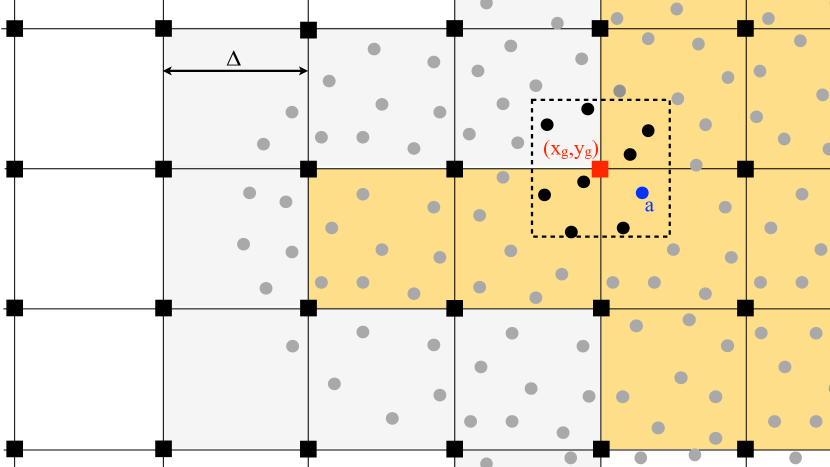
Figure 1: Sketch of a particle mesh configuration (for simplicity in 2D). Surface cells (at least one empty direct neighbour cell) are underlaid with grey, cells with all direct neighbour cells being non-empty, but with at least one empty next-to-direct neighbour cell are underlaid with orange. The volume assigned to the grid point at $(x_{g},y_{g})$ is indicated by the dashed square.

We map a quantity $A$ that is known at particle positions $r^{i}_{p}$ to the grid point $r^{i}_{g}$ via

$$A_{g}=A(\vec{r}_{g})=\frac{\sum_{p}V_{p}A_{p}\Psi_{g}(\vec{r}_{p})}{\sum_{p}V_{p}\Psi_{g}(\vec{r}_{p})},$$ (76)

where $V_{p}=\nu_{p}/N_{p}$ is a measure of the particle volume. We apply here a hierarchy of shape functions $\Psi$ of decreasing interpolation order depending on the filling status of the neighbouring cells. In all of the cases we use tensor products of 1D functions

$$\Psi(x,y,z)_{g}=\Phi\left(\frac{|x-x_{g}|}{\Delta}\right)\Phi\left(\frac{|y-y_{g}|}{\Delta}\right)\Phi\left(\frac{|z-z_{g}|}{\Delta}\right).$$ (77)

We have experimented with a number of different shape functions, starting from commonly used SPH kernels, each time monitoring how close a (low resolution) neutron star remains to its initial TOV solution when both the fluid and the metric are evolved (typically monitoring several dozen dynamical time scales). We find good results for the following hierarchy of 1D shape functions $\Phi$ (to be used in Eq.(77)):

• for cells with $fs=3$ and $fs=2$ we use [89]

  $$M^{{}^{\prime\prime\prime}}_{6}(q)=\left\{\begin{array}[]{lr}-\frac{1}{88}(q-1)\left[60q^{4}-87(q^{3}+q^{2})+88(q+1)\right]&q<1\\ \frac{1}{176}(q-1)(q-2)\left[60q^{3}-261q^{2}+257q+68\right]&1\leq q<2\\ -\frac{3}{176}(q-2)\left[4q^{2}-17q+12\right](q-3)^{2}&2\leq q<3\\ 0&{\rm else},\end{array}\right.$$

• for cells with $fs=1$ we use [90, 87]

  $$M^{{}^{\prime}}_{4}(q)=\left\{\begin{array}[]{lr}1-\frac{5}{2}q^{2}+\frac{3}{2}q^{3}&q<1\\ \frac{1}{2}(2-q)^{2}(1-q)&1\leq q<2\\ 0&{\rm else}\end{array}\right.$$

• and [86]

  $$M_{3}(q)=\left\{\begin{array}[]{lr}\frac{1}{2}(q+\frac{3}{2})^{2}-\frac{3}{2}(q+\frac{1}{2})^{2}&q<1/2\\ \frac{1}{2}(-q+\frac{3}{2})^{2}&1/2\leq q<3/2\\ 0&{\rm else}\end{array}\right.$$

  for cells with $fs=0$, i.e. for cells near the surface.

Note that, strictly speaking, with these choices the kernel support size can reach empty cells beyond a fluid surface, but in all of our tests we found good results with the chosen hierarchy. The kernels are plotted in Fig. 2. Note that out of these kernels, only $M_{3}$ is strictly positive definite.

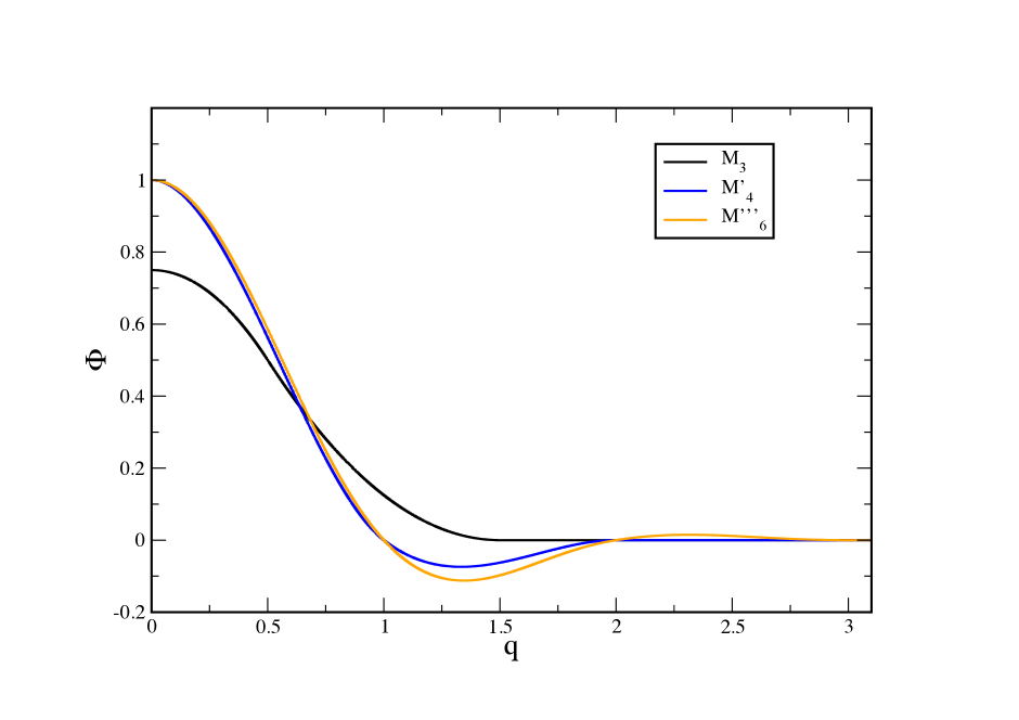
Figure 2: The shape functions used in the “particle-to-mesh” mapping step.

B. Moving Least Squares
As an alternative to using the above described method with pre-described kernels, we have also implemented a Moving Least Squares (MLS) approach to map the particle properties onto the mesh. The main idea is to assign a set of basis functions $\{b^{g}_{i}(x,y,z),i=1..m\}$ to each grid point labelled by $g$ and to determine the needed set of coefficients $\{c^{g}_{i},i=1..m\}$ by minimizing an error functional based on the particles in the neighbourhood of the grid point.
The function to be mapped to the mesh, optimized at a grid point, is then written as

$$\tilde{A}_{g}(\vec{r})=\sum_{i=1}^{m}c^{g}_{i}b_{i}(\vec{r}).$$ (78)

The local coefficients $c^{g}_{i}$ are determined by minimizing the error functional

$$\mathcal{L}(\{c^{g}_{i}\})\equiv\sum_{b}W(|\vec{r}_{g}-\vec{r}_{b}|)\left\{A_{b}-\sum_{i=1}^{m}c^{g}_{i}b_{i}(\vec{r}_{b})\right\}^{2}$$ (79)

with respect to the $c^{g}_{i}$. The function $W$ gives more weight to nearby than to far away particles and one can take, for example, a typical SPH-kernel. Requiring

$$0\stackrel{{\scriptstyle!}}{{=}}\frac{\partial\mathcal{L}}{\partial c^{g}_{i}}$$ (80)

yields the coefficients as

$$c^{g}_{i}=M_{ij}^{-1}\;d_{j},$$ (81)

where

$$M_{ij}=\sum_{b}W(|\vec{r}_{b}-\vec{r}_{g}|)\;b_{i}(\vec{r}_{b})\;b_{j}(\vec{r}_{b})$$ (82)

and

$$d_{j}=\sum_{b}=W(|\vec{r}_{b}-\vec{r}_{g}|)\;A_{b}\;b_{j}(\vec{r}_{b}).$$ (83)

In our approach we have chosen the basis functions $\{1,\tilde{x},\tilde{y},\tilde{z},\tilde{x}\tilde{x},\tilde{x}\tilde{y},\tilde{x}\tilde{z},\tilde{y}\tilde{y},\tilde{y}\tilde{z},\tilde{z}\tilde{z}\}$, where $\tilde{x}=x-x_{g},\tilde{y}=y-y_{g},\tilde{z}=z-z_{g}$, and a tensor-product version of the $M_{3}$ kernel as the positive-definite weight function. The required solution of a $10\times 10$ linear system involving the matrix $(M_{ij})$ is performed via a LU-decomposition (and a singular value decomposition [91] as fallback option) and this makes the MLS approach for the P2M-step about 10% more computationally expensive than the prescribed kernels, but in terms of the overall run time both approaches are very similar.

Mesh-to-Particle (M2P) step
Due to the regularity of a mesh, this step is somewhat simpler and we can draw on knowledge form mesh-based methods. An obvious choice would be to use exactly the same kernels as in the P2M-step. After many numerical experiments, we have settled, however, on two other methods, a WENO5-variant [92] and a quintic Hermite polynomial interpolation that are substantially more accurate; in particular near the stellar surface. In the following, we will concisely summarize these methods.

A. WENO 5
When interpolating some function, $A_{g}$, given at grid positions $\vec{r}_{g}$, to some general position $\vec{r}$, oscillations can occur when encountering sharp transitions. Whether they occur or not depends on the chosen stencil, and Weighted Essentially Non-Oscillatory (WENO) schemes are designed so that a suitably weighted superposition of stencils gives most weight to non-oscillatory stencils. Here we follow the suggestion of Kozak et al. [92] for such a scheme of fifth order (WENO5).
The task is now to “transfer” a function that is known on a grid ($A_{g}$) to a general position

$$A(\vec{r})=\sum_{g}\Phi_{g}(\vec{r})A_{g},$$ (84)

where the weight functions $\Phi_{g}$ form a partition of unity

$$\sum_{g}\Phi_{g}(\vec{r})=1.$$ (85)

Here, we also use tensor products of 1D-functions similar to Eq. (77). The scheme uses non-dimensional distances from the grid centres

$$\tilde{x}=\frac{x-x_{g}}{\Delta}\quad\tilde{y}=\frac{y-y_{g}}{\Delta}\quad\tilde{z}=\frac{z-z_{g}}{\Delta}$$ (86)

and the following linear weights for the left, central and right positions

$$C^{L} = \frac{1}{12}(\tilde{x}-1)(\tilde{x}-2);$$

$$C^{C} = -\frac{1}{6}(\tilde{x}+2)(\tilde{x}-2);$$ (87)

$$C^{R} = \frac{1}{12}(\tilde{x}+2)(\tilde{x}+1).$$

The following smoothness indicators are used

$$\beta^{L}_{j,k} = \frac{13}{12}(A_{0,j,k}-2A_{1,j,k}+A_{2,j,k})^{2}+\frac{1}{4}(A_{0,j,k}-4A_{1,j,k}+3A_{2,j,k})^{2}$$

$$\beta^{C}_{j,k} = \frac{13}{12}(A_{1,j,k}-2A_{2,j,k}+A_{3,j,k})^{2}+\frac{1}{4}(A_{1,j,k}-A_{3,j,k})^{2}$$ (88)

$$\beta^{R}_{j,k} = \frac{13}{12}(A_{2,j,k}-2A_{3,j,k}+A_{4,j,k})^{2}+\frac{1}{4}(3A_{2,j,k}-4A_{3,j,k}+A_{4,j,k})^{2}$$

and from them the auxiliary variables

$$\alpha^{M}_{j,k}=\frac{C^{M}}{(\beta^{M}_{j,k}+\epsilon)^{2}}$$ (89)

are calculated, where $M$ stands for either $L,C$ or $R$. These $\alpha^{M}_{j,k}$ are then in turn used for the non-linear weights

$$\omega^{M}_{j,k}=\frac{\alpha^{M}_{j,k}}{\sum_{I}\alpha^{I}_{j,k}},$$ (90)

where the $I$ summation runs over $L,C$ and $R$. The final weight function is then

$$\Phi^{\rm W5}(\tilde{x})=\left\{\begin{array}[]{lr}0&\tilde{x}<-\frac{5}{2}\\ \frac{1}{2}(\tilde{x}+1)\;\tilde{x}\;\omega^{L}_{j,k}&-\frac{5}{2}\leq\tilde{x}<-\frac{3}{2}\\ -(\tilde{x}+2)\;\tilde{x}\;\omega^{L}_{j,k}+\frac{1}{2}\tilde{x}\;(\tilde{x}-1)\;\omega^{C}_{j,k}&-\frac{3}{2}\leq\tilde{x}<-\frac{1}{2}\\ \frac{1}{2}(\tilde{x}+2)(\tilde{x}+1)\;\omega^{L}_{j,k}\\ -(\tilde{x}+1)(\tilde{x}-1)\;\omega^{C}_{j,k}&-\frac{1}{2}\leq\tilde{x}<\frac{1}{2}\\ +\frac{1}{2}(\tilde{x}-1)(\tilde{x}-2)\;\omega^{R}_{j,k}\\ \frac{1}{2}(\tilde{x}+1)\;\tilde{x}\;\omega^{C}_{j,k}-\tilde{x}\;(\tilde{x}-2)\;\omega^{R}_{j,k},&\frac{1}{2}\leq\tilde{x}<\frac{3}{2}\\ \frac{1}{2}\tilde{x}\;(\tilde{x}-1)\;\omega^{R}_{j,k}&\frac{3}{2}\leq\tilde{x}<\frac{5}{2}\\ 0&\tilde{x}>\frac{5}{2}\\ \end{array}\right.\\$$

B. 5th-order Hermite interpolation
If one where to use standard Lagrange Polynomial interpolation when mapping metric data from the grid to the particle positions, the particle would see a continuous but non-differentiable metric when crossing grid lines. To avoid the extra noise caused by this, we have implemented a 5th order Hermite interpolation scheme (following [93]) for the mapping of metric quantities from the grid to the particle positions.

Even in the presence of hydrodynamical shocks, the metric will be at least twice differentiable (i.e. $C^{2}$). By using Hermite interpolation we ensure that the interpolated values are $C^{2}$ across grid boundaries. In one dimension, on the interval $[x_{i},x_{i+1}]$, we therefore want to define an interpolating function, $f(x)$, that has the following properties:

$$f(x_{i})=f_{i}=C_{1}, f(x_{i+1})=f_{i+1}=C_{2},$$

$$f^{\prime}(x_{i})=f^{\prime}_{i}=C_{3} f^{\prime}(x_{i+1})=f^{\prime}_{i+1}=C_{4},$$ (91)

$$f^{\prime\prime}(x_{i})=f^{\prime\prime}_{i}=C_{5} f^{\prime\prime}(x_{i+1})=f^{\prime\prime}_{i+1}=C_{6}.$$

As we have six conditions to impose, $f(x)$ needs to be at least a 5th order polynomial. Introducing

$$\Delta x=x_{i+1}-x_{i}$$ (92)

and

$$\tilde{x}=\frac{x-x_{i}}{\Delta x}$$ (93)

we can write the interpolating quintic Hermite polynomial as

$$H_{5}(\tilde{x}) = f_{i}\,\psi_{0}(\tilde{x})+f_{i+1}\,\psi_{0}(1-\tilde{x})$$

$$+f^{\prime}_{i}\Delta x\,\psi_{1}(\tilde{x})+f^{\prime}_{i+1}\Delta x\,\psi_{1}(1-\tilde{x})$$

$$+f^{\prime\prime}_{i}\Delta x^{2}\,\psi_{2}(\tilde{x})+f^{\prime\prime}_{i+1}\Delta x^{2}\,\psi_{2}(1-\tilde{x}),$$

where the conditions on the function values and derivatives determine the 3 quintic Hermite basis functions

$$\psi_{0}(\tilde{x}) = -6\tilde{x}^{5}+15\tilde{x}^{4}-10\tilde{x}^{3}+1,$$

$$\psi_{1}(\tilde{x}) = -3\tilde{x}^{5}+8\tilde{x}^{4}-6\tilde{x}^{3}+\tilde{x},$$ (95)

$$\psi_{2}(\tilde{x}) = \frac{1}{2}(-\tilde{x}^{5}+3\tilde{x}^{4}-3\tilde{x}^{3}+\tilde{x}^{2}).$$

As we do not know the values of the first and second derivatives of the metric quantities at $x_{i}$ and and $x_{i+1}$, we approximate these by fourth order finite differences as

$$f^{\prime}_{i} = \frac{f_{i-2}-8f_{i-1}+8f_{i+1}-f_{i+2)}}{12\Delta x},$$ (96)

$$f^{\prime\prime}_{i} = \frac{-f_{i-2}+16f_{i-1}-30f_{i}+16f_{i+1}-f_{i+2}}{12\Delta x^{2}},$$ (97)

and similarly for the point $x_{i+1}$ with the stencil shifted by one. In one dimension the stencil for Hermite 5 interpolation thus becomes a six point stencil from $x_{i-2}$ to $x_{i+3}$ where the point, $x$, to be interpolated to lies in the interval $[x_{i},x_{i+1}]$.

In three dimensions the Hermite interpolation stencil consists of the 216 points in the 6x6x6 cube defined by the corners $(x_{i-2},y_{i-2},z_{i-2})$ and ($x_{i+3},y_{i+3},z_{i+3})$. The interpolation to point $(x,y,z)$ then proceeds in principle as 36 one dimensional interpolation in the $z$-direction to the points in the square defined by $(x_{i-2},y_{i-2},z)$ to $(x_{i+3},y_{i+3},z)$, then another six interpolations in the $y$-direction to the points on the line from $(x_{i-2},y,z)$ to $(x_{i+3},y,z)$ and finally a last interpolation in the $x$-direction to the point $(x,y,z)$.

In practice, however, we have prederived expressions for the weights of all 216 points in the three dimensional stencil, so when we know which point we have to interpolate to, we calculate the weights and then do the interpolations in all three directions in one go. This has the advantage, that we can reuse the weights for each function we have to interpolate to the same point.

2.5 Initial conditions and Artificial Pressure Method (APM)

Apart from the shock test described in Sec. 3.1, all other tests in these papers are concerned with the evolution of neutron stars. The initial neutron star profiles are obtained by solving the Tolman-Oppenheimer-Volkoff (TOV) equations [94, 95]. In setting up our initial configurations we have to take into account a peculiarity of SPH: its sensitivity to particles of different masses (Newtonian) or baryon numbers (relativistic case). Ideally, one would like to have initial particle distributions that a) are very regular (for a more quantitative definition of this property see Sec. 2 in [41]), b) do not contain preferred directions (which simple lattices usually do) and c) have equal masses/baryon numbers, i.e. the information about the density structure should be encoded in the particle position distribution (rather than in the masses/baryon numbers as is the case for regular lattices). In practice it can become a non-trivial task to set up particle distributions that fulfil these properties. It should be noted, however, that in particular stiff EOSs (e.g. $\Gamma=2.75$) with their nearly uniform densities can still be handled with a uniform lattice. For the resolutions shown in this paper, a uniform setup results in baryon number ratios of $\sim 8$ between center and the resolvable neutron star surface; which is perfectly acceptable. For $\Gamma=2.0$, however, this ratio becomes much larger ($>10^{4}$) and here a more sophisticated setup is beneficial.
For such a setup, we modify the “Artificial Pressure Method” (APM) that has recently been suggested in the context of the Newtonian SPH code MAGMA2 [71] for the case of relativistic TOV-stars. The main idea of the APM method is to distribute equal mass/baryon number particles, measure their current density according to Eq.(15) and then define an “artificial pressure” based on the relative deviation between the measured density and the desired profile density. This artificial pressure is used in a momentum-type equation similar to Eq.(19) to drive the equal mass particles iteratively into positions where they minimize the deviation from the desired density profile. What we use here is a straight-forward translation of the original Newtonian method. Here we briefly summarize the method and refer to the original paper for more details and tests.
Specifically, we follow the following steps:

• Distribute the initial guess of the particle positions. To this end we have implemented a regular cubic and a hexagonal lattice. The particles are placed in a sphere of radius $1.2R_{\rm NS}$, where $R_{\rm NS}$ is the radius of the TOV solution. The particles outside $R_{\rm NS}$ serve as boundary particles in the iteration process and are discarded once the iteration process has converged.

• In the next step we assign the artificial pressure $\Pi_{a}$ to particle $a$ according to

  $$\Pi_{a}\equiv{\rm max}\left[1+\frac{N_{a}-N^{\rm TOV}(\vec{r}_{a})}{N^{\rm TOV}(\vec{r}_{a})},0.1\right]$$ (98)

  and use it for the

• position update $\vec{r}_{a}\rightarrow\vec{r}_{a}+\delta\vec{r}_{a}^{\rm APM}$ where

  $$\delta\vec{r}_{a}^{\rm APM}=-\frac{1}{2}h_{a}^{2}\nu\sum_{b}\frac{\Pi_{a}+\Pi_{b}}{N_{b}}\nabla_{a}W_{ab}(h_{a}).$$ (99)

  As outlined above, this is a straight-forward translation of the Newtonian method, the details of which can be found in Sec. 3.1 of [71]. This update procedure tries to minimize the density error for the given baryon mass $\nu$ of all the particles, but it does not consider the regularity of the particle distribution. To achieve a good compromise between good density estimate (for the same $\nu$) and a locally regular particle distribution we add a regularization term similar to [44]

  $$\delta\vec{r}_{a}^{\rm reg}=h_{a}^{4}W_{ab}(h_{a})\hat{e}_{ab},$$ (100)

  so that the final position correction is

  $$\delta\vec{r}_{a}=(1-\zeta)\delta\vec{r}_{a}^{\rm APM}+\zeta\delta\vec{r}_{a}^{\rm reg}.$$ (101)

  After some experimenting we settled for a value of $\zeta=0.1$ for the regularization contribution.

• The SPH form of the hydrodynamic equations, Eq. (19), has excellent momentum conservation properties, but the gravitational acceleration terms that are calculated on a mesh and interpolated back to the particle positions can introduce a small momentum violation if the particles are not perfectly symmetrically distributed. As a thought experiment think of the star being composed of only two SPH particles: even if the accelerations are exactly the TOV values, this will result in a non-zero total momentum change unless the particles are symmetric with respect to the centre of the star. Therefore, we enforce perfect symmetry after each position update, simply by assigning to each of the first half of the particles a “mirror particle” that is symmetric with respect to the origin.

• To monitor the convergence, we measure the average density error and once it has not improved for 20 trial iterations, we consider the particle distribution as converged.

• Once this stage has been reached, we improve the agreement with the TOV-solution by now adjusting the particle masses in an iterative process. This leads to final ratios in the SPH particle baryon numbers of a few, which is perfectly acceptable. The exact ratio depends on how centrally condensed the stellar model is (i.e. on the equation of state) and we find ratios of $\sim 2$ for a stiff, $\Gamma=2.75$, and ratios of $\sim 6$ for a softer, $\Gamma=2.0$, equation of state (compared to ratios $>10^{4}$ for straight-forward lattice setup).

Note that with our setup we try to closely approximate the density distribution, the exact baryon mass is not actively enforced and can therefore be used as a consistency check. We find that it agrees very well with the one from the TOV profile, typically to $\sim 0.2$ % for stars with a few hundred thousand particles. An example of initial particle distributions ($|z|<0.5$, 100k particles) of a $\Gamma=2.0$ equation of state is shown in Fig. 3. The left panel shows a hexagonal lattice while the right panel shows a setup according to the APM (max./min. baryon number for this case $\sim 6$).

Figure 3: Particle distribution ($|z|<0.5$) according to a uniform hexagonal lattice (left) and according to the Artificial Pressure Method (APM), see main text for more details.

2.6 Code Implementation

Apart from the used McLachlan thorn [81] (described in the spacetime section above) our code has been written entirely from scratch in modern Fortran (with elements up to Fortran 2008). Since SPHINCS_BSSN has been written alongside the high-precision SPH code MAGMA2 [71], both codes share some modules such as the kernel calculation and parts of the tree-infrastructure for the neighbour search. SPHINCS_BSSN will be developed further in the near future. In its current stage it is OpenMp parallelized and it takes about 10 hours of wall clock time on an Intel Cascade Lake Platinum 9242 (CLX-AP) node to evolve 1 million particles together with a $300^{3}$ uniform mesh for a physical time of 1 ms. For now, a uniform mesh is implemented, but this may be improved in the future.

3 Tests

All tests shown here are performed with the full 3+1 dimensional hydrodynamics code. We have run a very large set of experiments where we evolved TOV neutron stars (hydrodynamics and spacetime) and we monitored how close the solution remained to the 1D TOV-solution for different combinations of our numerical choices. After these tests we settled on the following default choices: the sequence $MLS-MLS-MLS-M_{3}$ (from $fs=3$ to 0) for the P2M-mapping and 5th order Hermite interpolation for the P2M-mapping. We use $\alpha_{0}=0.1$ as minimum and 1.5 as the maximum dissipation value. But note that a number of other combinations yield very similar results. For example, $M^{{}^{\prime\prime\prime}}_{6}-M^{{}^{\prime\prime\prime}}_{6}-M_{4}-M_{3}$ works nearly as well and is computationally slightly cheaper, though the P2M-step is only a moderate fraction of the overall computational time.
Our code uses units with $G=c=1$ and masses are measured in solar units. Unless units are explicitly provided, all parameters given for initial data are in code units. These are often useful because the initial conditions of many tests that we show are given in the literature also in these units. However, for the physical results related to neutron stars, we prefer to use physical (cgs-)units, but we believe that this use of units should not lead to any confusion.

3.1 Relativistic shock tube

In this first test we scrutinize the ability of our full-GR code to correctly reproduce the special-relativistic hydrodynamics limit. The test is a relativistic version of “Sod’s shocktube” [96] which has become a widespread benchmark for relativistic hydrodynamics codes [97, 74, 68, 98, 99]. The test uses a polytropic exponent $\Gamma=5/3$ and as initial conditions

$$\left[N,P\right]=\left\{\begin{array}[]{ll}\left[10,\frac{40}{3}\right],&{\rm for\;}x<0\\ \left[1,10^{-6}\right]&{\rm for\;}x\geq 0,\end{array}\right.$$ (102)

with velocities initially being zero everywhere. We place particles with equal baryon numbers on close-packed lattices as described in [66], so that on the left side the particle spacing is $\Delta x_{L}=0.0005$ and we have 12 particles in both y- and z-direction. This test is performed with the full 3+1 dimensional code, but using a fixed Minkowski metric. The result at $t=0.15$ is shown in Fig. 4 with the SPHINCS_BSSN results marked with blue squares and the exact solution [99] with the red line. Overall there is very good agreement with practically no spurious oscillations.

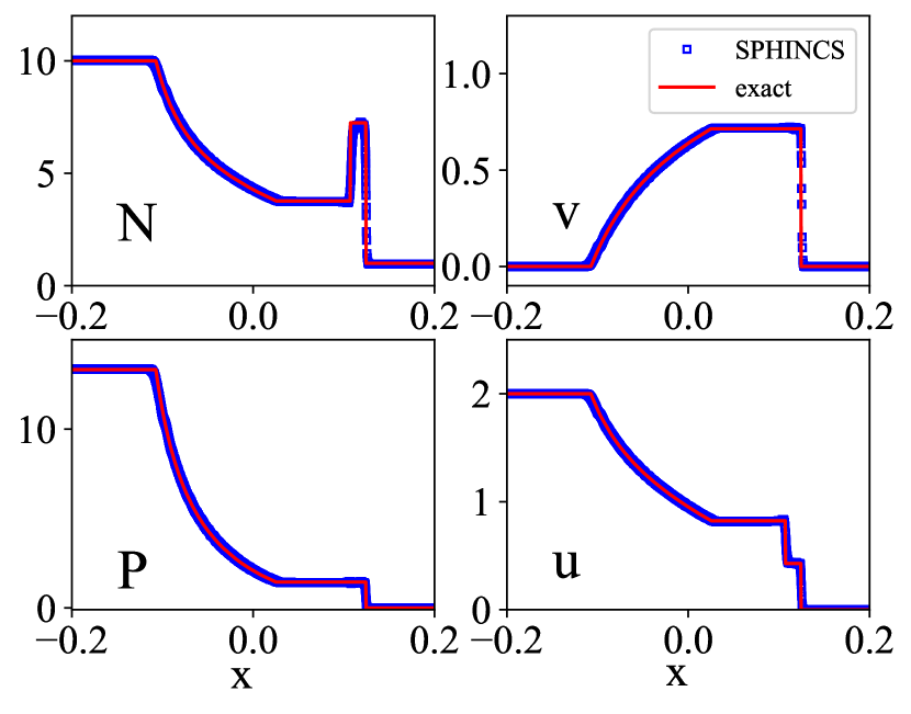
Figure 4: Result of a 3D relativistic shock tube (initial particle spacing on the left $\Delta x_{L}=0.0005$) at t= 0.15, numerical results are shown as blue squares, the exact solution is shown in red.

To illustrate the effect of the reconstruction in the artificial dissipation we repeat this 3D test at low resolution ($\Delta x_{L}=0.003$), once without, once with reconstruction in only $V$ and once with reconstruction in $V$ and $u$, see Fig. 5.

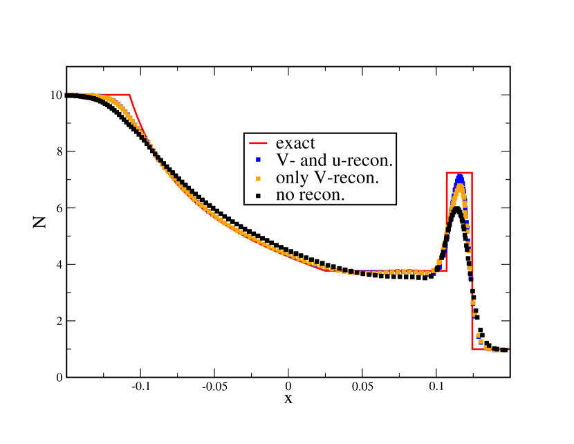
Figure 5: Result of a low resolution 3D relativistic shock tube (initial particle spacing on the left $\Delta x_{L}=0.003$) at t= 0.15. The exact solution is shown in red, the numerical solution without any reconstruction in black, with reconstruction in only $V$ in orange and with reconstruction in both $V$ and $u$ in blue.

3.2 Hydrodynamic evolution of neutron star in a static metric (“Cowling approximation”)

After testing the special-relativistic performance of the hydrodynamic terms in the previous shock test, we next test the general-relativistic hydrodynamics by evolving the matter variables of a neutron star while keeping the metric fixed (“Cowling approximation”). The purpose of this test is two-fold: a) it should demonstrate that the 3D star remains close to the initial solution that has been found by solving the 1D TOV-equations and b) we will measure oscillation frequencies and compare them to results from the literature. To enable a straight-forward comparison we follow here the setup of [100] who also provide their results for the oscillation frequencies. We model a 1.40 M_⊙ (gravitational mass) neutron star by solving the TOV equations with a $\Gamma=2.00$ polytropic exponent, a prefactor of $K=100$ in the polytropic equation of state, $P=Kn^{\Gamma}$, and a central density of $\rho_{c}=1.28\times 10^{-3}$.
We set up initial TOV stars according to the APM described in Sec. 2.5 at three different resolutions: 250k, 500k and 1M particles. Note that in Newtonian SPH one usually “relaxes” a star to find its true numerical equilibrium. This is usually done, see e.g. [19], by setting up the particles as closely to the hydrostatic equilibrium as possible and then let them evolve with some extra-dissipation, so that they can settle locally into an ideal particle configuration. We do not perform such a relaxation step here, but start directly with the stars from the APM setup. Therefore, in the initial phase the particles will try to further optimize their local arrangement in addition to a possible bulk motion. To set the star into oscillation we apply a small radial perturbation

$$\delta v^{r}=\delta v_{0}\sin\left(\frac{\pi r}{R}\right),$$ (103)

where $\delta v_{0}=0.005$.
The evolution of the central densities of these stars over $\approx 15$ ms is shown in Fig. 6. Overall, the stars at all resolutions stay close to the initial TOV solution and stably oscillate around it without noticeable systematic drift. The oscillations are somewhat damped by numerical viscosity, but notably less so with increasing resolution.

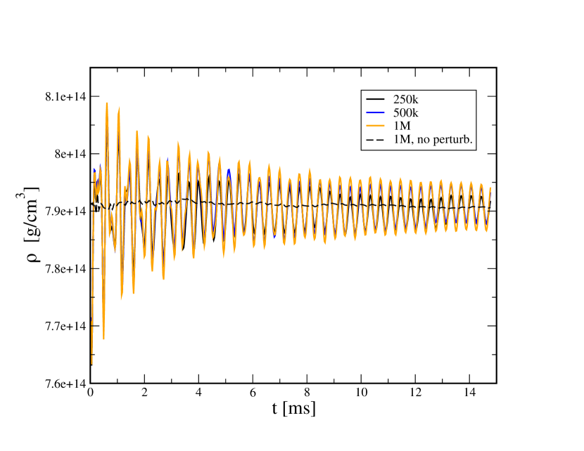
Figure 6: Central density oscillations of three stars (250k, 500k and 1M SPH particles) in Cowling approximation with a $\Gamma=2.0$ polytropic equation of state. The oscillations have been triggered by a small velocity perturbation $\delta v_{0}=0.005$. We also show a case where no explicit perturbation was applied (black dashed line).

We also measure the oscillation frequencies and present the resulting Fourier spectrum in Fig. 7. We find excellent agreement with the values for the fundamental normal mode (F: 2.696 kHz) and the first two overtones (H1: 4.534 kHz, H2: 6.346 kHz) determined in [100] using a 3D Eulerian high resolution shock capturing code. The spectrum agrees well among the three resolutions and as expected, the peaks get sharper and have higher amplitudes at higher resolution. Higher order overtones are excited at a too low amplitude to be visible in the spectrum.

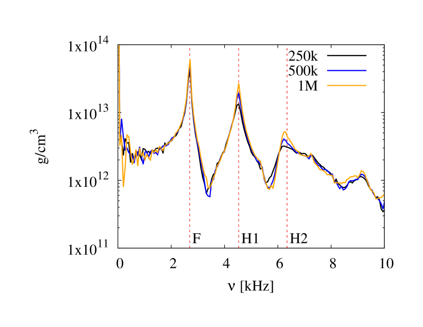
Figure 7: Fourier spectrum of the central density oscillations of the three stars shown Fig. 6 that have been evolved in the ”Cowling approximation” (matter is evolved, but spacetime held fixed). Also indicated with the red dashed vertical lines are the fundamental normal mode frequency (F) and the next two higher mode frequencies (H1, H2) as determined by [100] in a 3D study.

3.3 Stable neutron star with dynamical spacetime evolution

As the next step, we take the configuration from the previous test, but now also evolve the spacetime dynamically, i.e. we are testing the general relativistic hydrodynamics, the spacetime evolution and their coupling. During the subsequent numerical evolution, the neutron star should remain stable and close to the initial TOV setup. As a further test, we measure again the oscillation frequencies of the star and compare them against the results published in [100].
We use a setup very similar to the previous test and use in particular (unrelaxed) initial configurations with 250k (grid resolution $126^{3}$), 500k ($151^{3}$) and 1M particles ($191^{3}$ grid points). The number of grid points has been chosen so that the average number of particles per grid cell is approximately the same ($\approx 15$). We slightly perturb the stars according to Eq. (103). The evolution of the central densities are shown in Fig. 8.

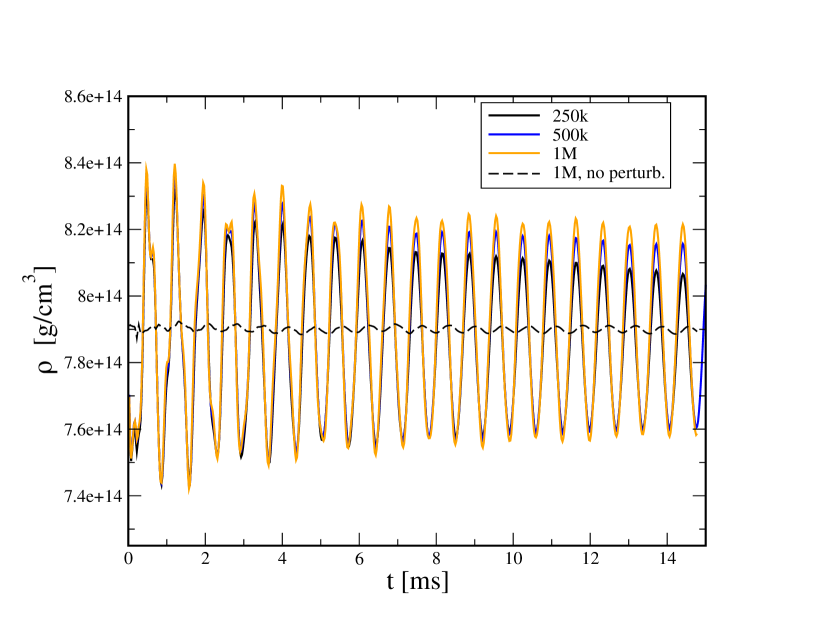
Figure 8: Central density oscillations in the full matter+spacetime evolution of a neutron star. The initial model is set up according to the TOV equations with a polytropic exponent $\Gamma=2.00$ The used SPH particle numbers are indicated in the legend (“k”: thousands, “M”: million), the spacetime was evolved on a grid covering a volume of $[-30,30]^{3}$ (in code units; 1 length code unit= 1.47676 km). See main text for more details. The solid lines show cases where the oscillations were triggered with a small velocity perturbation, the thin dashed line shows the result for 1 million particles where no explicit velocity perturbation was applied and the oscillations are triggered exclusively by truncation error.

Again the stars oscillate stably around the initial TOV central density and with only moderate decrease in oscillation amplitude due to dissipative effects. As expected, and as seen before, the dissipation decreases further with increasing resolution.
We measure again the oscillation frequencies and present them in Fig. 9. Once more, we find excellent agreement with the values for the fundamental normal mode (F: 1.450 kHz) and the first two overtones (H1: 3.958 kHz, H2: 5.935 kHz) from [100]. As in the Cowling case, higher overtones are excited at too low amplitudes to be seen reliably in the spectrum. However, there might be a small hint of H3 at 7.812 kHz.

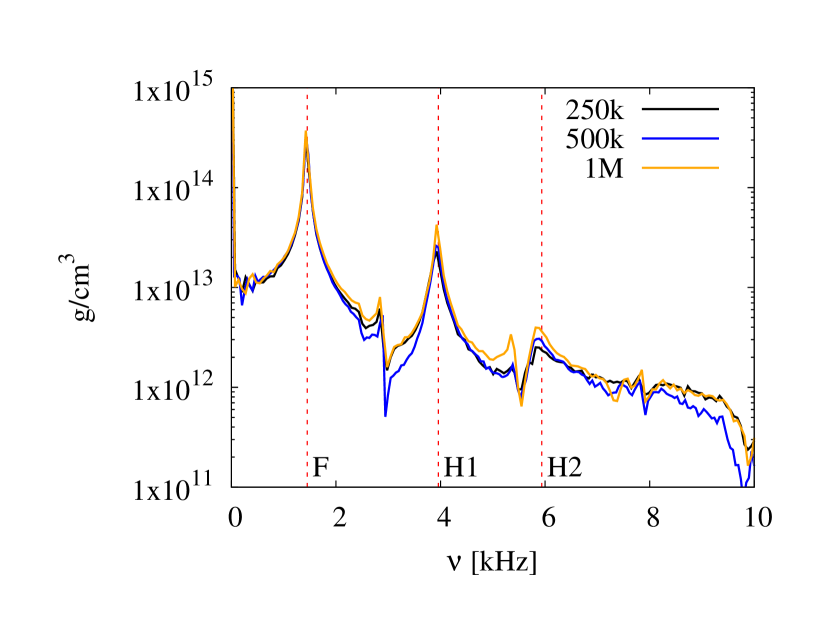
Figure 9: Fourier spectrum of the central density oscillations of neutron stars that were self-consistently evolved together with the spacetime, see Fig. 8. Also indicated with the red dashed vertical lines are the fundamental normal mode frequency (F) and the next two higher mode frequencies (H1, H2) as determined by [100].

In Fig. 10 (left panel) we show the particle distribution of a $\Gamma=2.0$ star (no initial velocity perturbation; shown as black dashed line in Fig. 8) after it has been evolved (hydrodynamics and spacetime) for $10.2$ ms. Note that, contrary to Eulerian General Relativity approaches, the neutron star surface does not pose any particular challenge for our numerical method: the surface remains sharp and perfectly well-behaved. In Fig. 10 (right panel) we show the radial structure of the density at time $0$ ms and $10.2$ ms. Note that during the 10 ms evolution the particles at the surface have slightly adjusted their positions compared to our initial setup and sit now at a slightly lower radius, but apart from that the radial density structure of the star after 10 ms is practically identical to the initial condition.

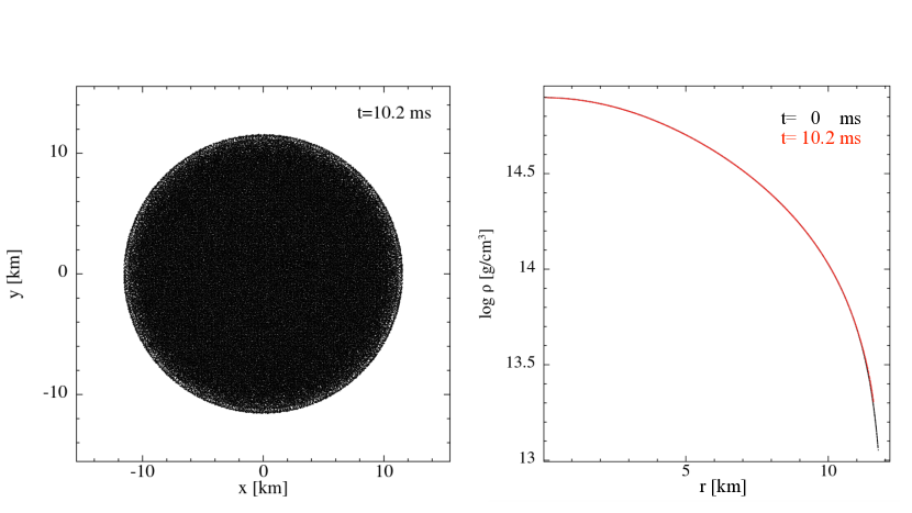
Figure 10: TOV neutron star ($\Gamma=2.0$) after it has been evolved (hydrodynamics and spacetime) for 10.2 ms. Only in the surface layers have the particle positions slightly adjusted, otherwise the star remained essentially perfectly on its initial condition. Note in particular that the stellar surface –which does not need any special treatment in our approach– has remained perfectly well-behaved.

3.4 Migration of an unstable neutron star to the stable branch

A more complex test case involves an unstable initial configuration of a neutron star [100, 101, 102]. Depending on the type of perturbation, such a star can either expand, collapse to a black hole or migrate to the stable branch of the sequence of equilibrium stars. In the latter case, the energy difference between the two configurations causes large-scale pulsations while the star transitions to the stable branch.
This test is very challenging for a number of reasons. The initial neutron star is highly relativistic with $\rho_{c}\approx 5\times 10^{15}$ g/cm³ and a central lapse $\alpha_{c}<0.3$. In the subsequent evolution the star expands by about a factor of three in radius while its central density drops by about a factor of 30. Thereafter it re-collapses and re-expands repeatedly with each cycle resulting in the formation of shocks which eject particles reaching velocities exceeding 0.6 times the speed of light and which unbind a non-negligible amount of the initial stellar mass. The test is also challenging for purely numerical reasons, especially when uniform grids are involved, since on the one hand the matter evolution should be followed far enough out so that ejecta can be clearly separated from matter falling back and, on the other hand, the initial star is highly centrally concentrated so that short length scales need to be resolved near the stellar centre. Clearly, this complex evolution involving strong gravity dynamically coupled to the hydrodynamic evolution, shock formation, matter ejection and fallback is far beyond the possibilities of any linear approximation.
For the initial conditions we follow the setup described in [102] and start from a solution of the TOV-equations with a polytropic equation of state, $P=Kn^{\Gamma}$ with exponent $\Gamma=2$ and $K=100$ and subsequently evolved using Eq. (45). With a central density of $7.993\times 10^{-3}$ the star has gravitational mass of 1.448 and an (isotropic coordinate) radius of $R=5.838$. The transition is triggered just by truncation error. We setup the star according to the APM with 1M particles, use a $301^{3}$ grid extending from -50 to 50 in each dimension and apply sixth order finite differencing in BSSN. The density evolution is shown in Fig. 11. The star rapidly expands by about a factor of three, then recollapses, forms a shock wave that is travelling outward and unbinding matter, recollapsing and so on. When we stop the simulation at $t\approx 5$ ms, about 0.099 M_⊙ have become unbound (particles were removed at a radius of 45). The corresponding evolution of the peak density (normalized to the initial value) is shown in Fig. 12, it agrees well with the results obtained by other methods [100, 101, 102]. We have further performed test calculations with only $201^{3}$ grid points to explore the impact of the finite difference order in the BSSN part. The results for order four, six and eight are shown in Fig. 12 as red, green and blue lines. The fourth order case shows somewhat lower peaks, which probably indicates that the steep central gradients are not resolved well enough. The other cases give nearly identical results.

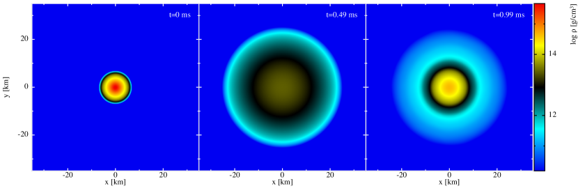
Figure 11: Density evolution in the migration test. In this test a highly relativistic neutron star is initially placed the unstable branch of the sequence of equilibrium stars, then undergoes large scale oscillations and finally settles on the stable branch. Please see main text for more details.

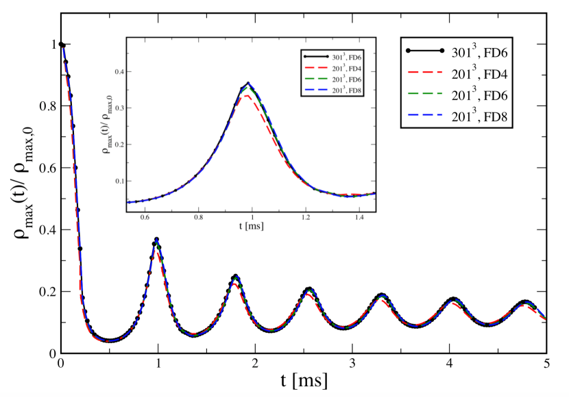
Figure 12: Evolution of the peak density (normalized to the initial peak density) in the migration test. Our default in this test (black line) was performed with 1 million particles and a $301^{3}$ grid extending from -50 to 50 in each dimension and with finite differencing order 6 (“FD6”). We performed additional tests, also with 1 million particles, but with a $201^{3}$ grid where we varied the finite difference order from 4 to 8.

3.5 Collapse of a neutron star to a black hole

In this test we simulate the collapse of an unstable neutron star into a black hole. We start from the same initial conditions as in Sec. 3.4. As mentioned there, this configuration is unstable and depending on the perturbation, it may either -via violent oscillations- transition to the stable branch or, otherwise, collapse into a black hole. As demonstrated above, truncation error alone triggers the transition to the stable branch, but only a small additional (momentum constraint violating) velocity perturbation is enough to change the subsequent evolution and to trigger the collapse to a black hole. Similar to Sec. 3.2, we apply a radial velocity perturbation

$$\delta v^{r}=-0.005\sin\left(\frac{\pi r}{R}\right),$$ (104)

where $R$ is the stellar radius.
For this test, we use a $401^{3}$ grid with boundaries at $x_{\rm BD}=y_{\rm BD}=z_{\rm BD}=15$, 6th order finite differencing and 900k SPH particles, set up according to the artificial pressure method, see Sec. 2.5. Black hole formation goes along with a ”collapse of the lapse”, i.e. the lapse $\alpha$ is dropping to zero in a region inside the horizon. To prevent the hydrodynamic evolution from failing close to the forming black hole singularity, we remove SPH particles that have a lapse value $\alpha<\alpha_{\rm thr}=0.03$.
We find that the small initial velocity perturbation triggers a rapid contraction of the neutron star which goes along with an increase in the density, see Fig. 13. We also show the evolution of the lapse (along the $x$-axes) for various time slices in Fig. 14. This ”collapse of the lapse” is characteristic for the formation of a black hole.

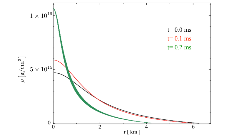
Figure 13: Density distribution in the collapsing neutron star test (initial condition is shown in black, the density at $t=0.1$ ms in red and at $t=0.2$ ms in green). The collapse is triggered by a small radial velocity perturbation. The test is performed with $401^{3}$ grid points and 900k SPH particles.

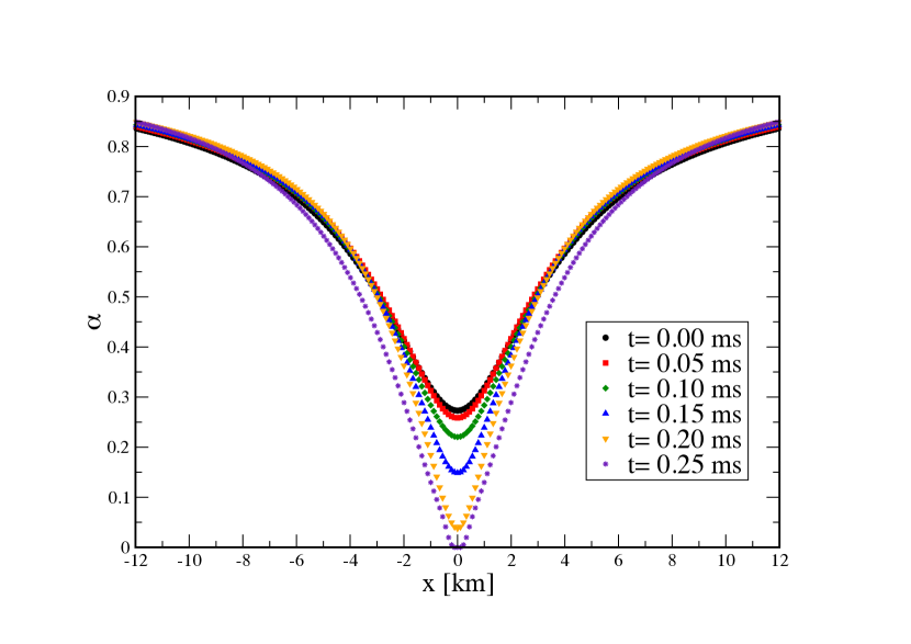
Figure 14: Evolution of the lapse function $\alpha$ along the $x$-axis for the unstable neutron star. The ”collapse of the lapse” is characteristic for the formation of a black hole.

In order to make sure, that the region where we remove particles (defined by the lapse threshold $\alpha_{\rm thr}$) is well contained within the event horizon, we imported our metric data into the Einstein Toolkit [82, 83] in order to apply the apparent horizon finder AHFinderDirect of [103] to our data, see Fig. 15. We find an apparent horizon for the first time shortly after 0.205 ms (the zero values before that simply indicate that no apparent horizon was found) with an irreducible mass close to 1.24 M_⊙ which grows initially, reaches a maximum value of 1.4314 M_⊙, decreases slightly and then starts to increase again until the end of the simulation.

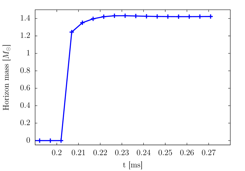
Figure 15: Evolution of the apparent horizon mass for the test with a collapsing neutron star.

In Fig. 16 we show the lapse profile at the time when the apparent horizon is first found. The vertical dashed red lines show the location of the apparent horizon. As the event horizon is guaranteed to be outside the apparent horizon at all times, we do have enough grid resolution, so that the removal of SPH particles (where $\alpha<\alpha_{\rm thr}$) can not affect the region outside the horizon. As can be seen from Fig. 16 in [104] the event horizon forms typically up to 1 ms before the apparent horizon and grows rapidly in size. Therefore, the fact that we start removing particles slightly before ($\approx$ 0.01 ms) the apparent horizon forms, is not a cause for concern. All particles were significantly inside of the horizon at the time of their removal.

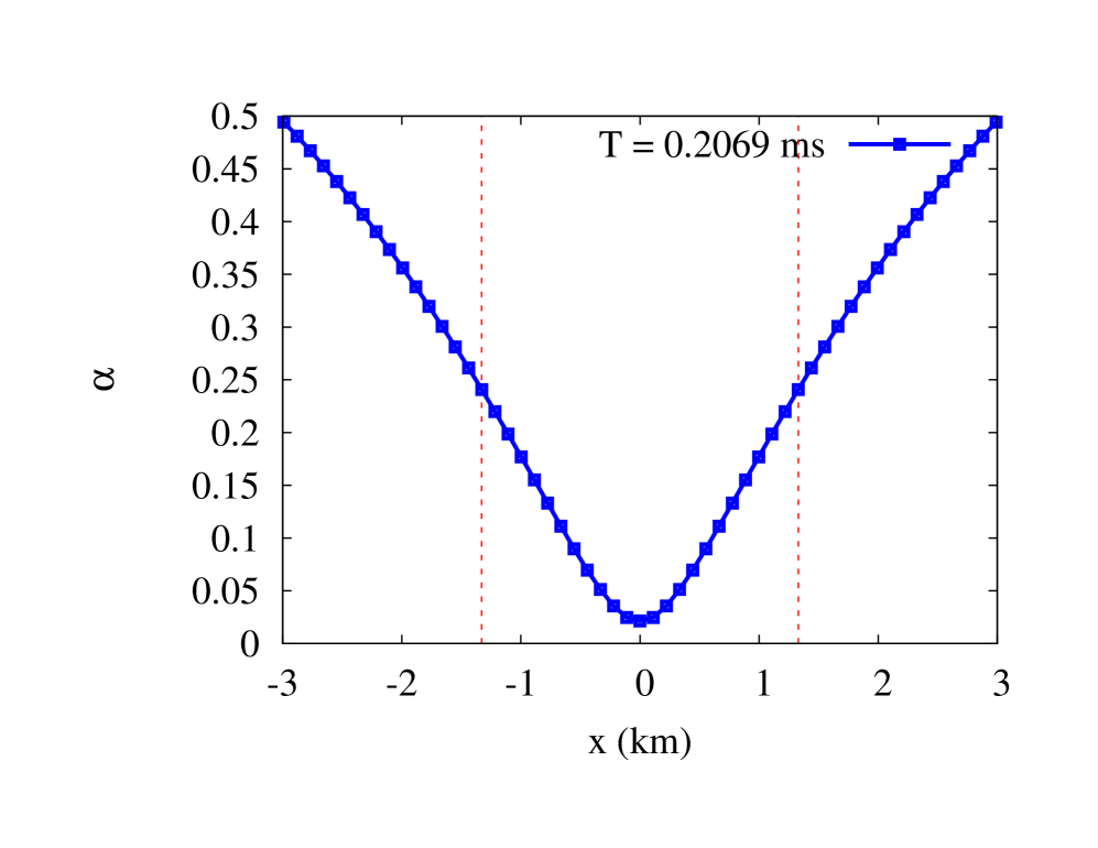
Figure 16: Lapse profile at the time of first finding the apparent horiozn. The vertical dashed lines show the size of the apparent horizon. The squares indicate the location of our grid points.

4 Summary and conclusions

In this paper we have presented the methodology behind what, to the best of our knowledge, is the first Lagrangian fully General Relativistic hydrodynamics code. Part of the motivation for our alternative approach comes from the recent breakthrough in multi-messenger astrophysics where a neutron star merger was observed both in gravitational and electromagnetic waves. While the gravitational waves are dominated by the bulk matter motion in the densest, innermost regions of the remnant, the electromagnetic emission is caused by comparatively small amounts of matter that are ejected from the merger site. Such ejecta pose a serious challenge to Eulerian methods, but are comparably straight forward to evolve in a Lagrangian approach such as ours.
In our new code SPHINCS_BSSN we evolve the matter by means of Lagrangian particles according to a General Relativistic Smoothed Particle Hydrodynamics (SPH) formulation, see Sec. 2.2. This formulation profits from a number of recent major improvements that have been discussed and extensively tested in a non-relativistic context and implemented in the MAGMA2 code [71]. The improvements include the use of high order Wendland kernel functions, a slope-limited reconstruction in the dissipation tensor, and a novel steering of the artificial dissipation by means of monitoring the exact conservation of entropy [75].
Relativistic gravity enters the fluid equations of motion via (derivatives and the determinant of) the metric tensor. We evolve the metric, see Sec. 2.3, like in most Eulerian hydrodynamics formulations by following the Baumgarte-Shapiro-Shibata-Nakamura (BSSN) approach [59, 60, 61]. For now, we solve the BSSN equations on a uniform Cartesian grid and calculate derivates via finite differencing (of either 4th, 6th or 8th order).
An important element of our approach is the coupling between the fluid (on particles) and the spacetime (known on a mesh), see Sec. 2.4. At every (sub-)step the energy-momentum tensor $T_{\mu\nu}$ of the fluid needs to be mapped from the particles to the grid points ($P2M$) and the metric tensor properties need to be mapped back to the particle positions ($M2P$). Both of these steps turned out to be crucial for the accuracy of our scheme. We found in particular that a straight forward mapping with SPH kernels in the $P2M$-step was not a good choice. Instead, we used a number of more accurate (but not strictly positive definite) kernels that have been developed in the context of vortex-particle methods. In addition, we have implemented a mapping via a Moving Least Square (MLS) method which requires the frequent solution of $10\times 10$ equation system. While this comes at some computational cost, it is still acceptable in the overall computational balance. Also for the $M2P$-step we have implemented several options including a weighted essentially non-oscillatory interpolation of order 5 (WENO5) and a 5th-order Hermite interpolation (inspired by and extending the work of Timmes and Swesty [93]). We found several mapping combinations to work well and we have chosen as defaults the MLS method in the $P2M$ and the 5th-order Hermite interpolation in the $M2P$ step.
A number of our test cases involves neutron stars which we set up according to a relativistic version of the ”Artificial Pressure Method” (APM) that has recently been suggested in a Newtonian context [71]. Its main purpose is to obtain a particle distribution that reflects a given density profile, see Sec. 2.5. Starting from some initial SPH particle distribution, an iteration is performed that drives the particles into locations where they minimize their density error. This is achieved by an Euler-type equation which uses an ”artificial pressure” that is based on a local density error measure.
We have scrutinized our methodology and implementation via a number of standard tests that are often used for Eulerian Numerical Relativity codes, see Sec. 3. All tests were performed with the full 3+1 code. We have tested the special-relativistic hydrodynamics part via a relativistic shock tube benchmark, the general-relativistic hydrodynamics by evolving a neutron star in a fixed spacetime (”Cowling approximation”) and, in a next step, we evolved the hydrodynamics together with the metric. In both of the latter cases the neutron stars remain very close to the exact TOV-solution and they oscillate at frequencies that are in excellent agreement with those found in semi-analytic and Eulerian approaches. Contrary to the latter approaches, the neutron star surface does not pose any challenge for SPHINCS_BSSN, it remains sharp throughout the evolution, see e.g. Fig. 10, and does not require any special treatment. We further present our results for the challenging ”migration test” where, triggered by truncation error alone, an unstable neutron star transitions via violent oscillations into a stable configuration. And finally, when a small velocity perturbation is added to the same neutron star, it collapses and forms a black hole. In all of these tests, we obtain results that are in very good agreement with those of established Eulerian Numerical Relativity codes.

5 Appendix A

The so-called ”W-method” [84, 85] also starts from the ADM variables $\gamma_{ij}$, $K_{ij}$, $\alpha$ and $\beta^{i}$ and defines the BSSN variables as

$$W = \gamma^{-1/6},$$ (105)

$$\tilde{\gamma}_{ij} = W^{2}\gamma_{ij},$$ (106)

$$K = \gamma^{ij}K_{ij},$$ (107)

$$\tilde{\Gamma}^{i} = \tilde{\gamma}^{jk}\tilde{\Gamma}^{i}_{jk},$$ (108)

$$\tilde{A}_{ij} = W^{2}\left(K_{ij}-\frac{1}{3}\gamma_{ij}K\right).$$ (109)

These quantities are evolved according to

$$\partial_{t}W = \frac{1}{3}W\left(\alpha K-\partial_{i}\beta^{i}\right)+\beta^{i}\bar{\partial}_{i}W,$$ (110)

$$\partial_{t}\gamma_{ij} = -2\alpha\tilde{A}_{ij}+\tilde{\gamma}_{ik}\partial_{j}\beta^{k}+\tilde{\gamma}_{jk}\partial_{i}\beta^{k}$$ (111)

$$-\frac{2}{3}\tilde{\gamma}_{ij}\partial_{k}\beta^{k}+\beta^{k}\bar{\partial}_{k}\tilde{\gamma}_{ij},$$

$$\partial_{t}K = -W^{2}\left(\tilde{\gamma}^{ij}\left[\partial_{i}\partial_{j}\alpha-\frac{1}{W}\partial_{i}W\partial_{j}\alpha\right]-\tilde{\Gamma}_{\mathrm{(n)}}^{i}\partial_{i}\alpha\right)$$ (112)

$$+\alpha\left(\tilde{A}^{i}_{j}\tilde{A}^{j}_{i}+\frac{1}{3}K^{2}\right)+\beta^{i}\bar{\partial}_{i}K+4\pi\alpha(\rho+s),$$

$$\partial_{t}\tilde{\Gamma}^{i} = -2\tilde{A}^{ij}\partial_{j}\alpha+\tilde{\gamma}^{jk}\partial_{j}\partial_{k}\beta^{i}+\frac{1}{3}\tilde{\gamma}^{ij}\partial_{j}\partial_{k}\beta^{k}$$ (113)

$$+2\alpha\left(\tilde{\Gamma}^{i}_{jk}\tilde{A}^{jk}-\frac{2}{3}\tilde{\gamma}^{ij}\partial_{j}K-\frac{3}{W}\tilde{A}^{ij}\partial_{j}W\right)$$

$$-\tilde{\Gamma}_{\mathrm{(n)}}^{j}\partial_{j}\beta^{i}+\frac{2}{3}\tilde{\Gamma}_{\mathrm{(n)}}^{i}\partial_{j}\beta^{j}+\beta^{j}\bar{\partial}_{j}\tilde{\Gamma}^{i}$$

$$-16\pi\alpha\tilde{\gamma}^{ij}s_{j},$$

$$\partial_{t}\tilde{A}_{ij} = W^{2}[-\partial_{i}\partial_{j}\alpha+\tilde{\Gamma}^{k}{ij}\partial_{k}\alpha+\alpha R_{ij}$$ (114)

$$-(\partial_{i}\alpha\partial_{j}W+\partial_{j}\alpha\partial_{i}W)]^{\mathrm{TF}}$$

$$+\alpha(K\tilde{A}_{ij}-2\tilde{A}_{ik}\tilde{A}^{k}_{j})+\tilde{A}_{ik}\partial_{j}\beta^{k}$$

$$+\tilde{A}_{jk}\partial_{i}\beta^{k}-\frac{2}{3}\tilde{A}_{ij}\partial_{k}\beta^{k}+\beta^{k}\bar{\partial}_{k}\tilde{A}_{ij}$$

$$-W^{2}\alpha 8\pi\left(T_{ij}-\frac{1}{3}\gamma_{ij}s\right),$$

where $\rho$, $s$ and $s_{i}$ are given by Eqs. (64)-(66). Finally $R_{ij}=\tilde{R}_{ij}+R^{W}_{ij}$, where $\tilde{R}_{ij}$ is given as for the $\phi-$method, while

$$R^{W}_{ij} = \frac{1}{W}\partial_{i}\partial_{j}W-\frac{1}{W^{2}}\partial_{i}W\partial_{j}W+2\tilde{\Gamma}^{k}_{ij}\partial_{k}W$$ (115)

$$+\tilde{\gamma}_{ij}\tilde{\gamma}^{kl}\left(\frac{1}{W}\partial_{i}\partial_{j}W-\frac{1}{W^{2}}\partial_{i}W\partial_{j}W+2\tilde{\Gamma}^{k}_{ij}\partial_{k}W\right)$$

$$+\frac{1}{W^{2}}\partial_{i}W\partial_{j}W-\tilde{\gamma}_{ij}\tilde{\gamma}^{kl}\frac{1}{W^{2}}\partial_{k}W\partial_{l}W.$$

References

- [1] B. P. Abbott, R. Abbott, T. D. Abbott, M. R. Abernathy, F. Acernese, K. Ackley, C. Adams, T. Adams, P. Addesso, R. X. Adhikari, and et al. Observation of Gravitational Waves from a Binary Black Hole Merger. Physical Review Letters, 116(6):061102, February 2016.
- [2] B. P. Abbott, R. Abbott, T. D. Abbott, F. Acernese, K. Ackley, C. Adams, T. Adams, P. Addesso, R. X. Adhikari, V. B. Adya, and et al. GW170817: Observation of Gravitational Waves from a Binary Neutron Star Inspiral. Physical Review Letters, 119(16):161101, October 2017.
- [3] B. P. Abbott, R. Abbott, T. D. Abbott, F. Acernese, K. Ackley, C. Adams, T. Adams, P. Addesso, R. X. Adhikari, V. B. Adya, and et al. Multi-messenger Observations of a Binary Neutron Star Merger. ApJL, 848:L12, October 2017.
- [4] B. P. Abbott, R. Abbott, T. D. Abbott, F. Acernese, K. Ackley, C. Adams, T. Adams, P. Addesso, R. X. Adhikari, V. B. Adya, and et al. Gravitational Waves and Gamma-Rays from a Binary Neutron Star Merger: GW170817 and GRB 170817A. ApJL, 848:L13, October 2017.
- [5] A. Goldstein, P. Veres, E. Burns, M. S. Briggs, R. Hamburg, D. Kocevski, C. A. Wilson-Hodge, R. D. Preece, S. Poolakkil, O. J. Roberts, and many more. An Ordinary Short Gamma-Ray Burst with Extraordinary Implications: Fermi-GBM Detection of GRB 170817A. ApJL, 848:L14, October 2017.
- [6] V. Savchenko, C. Ferrigno, E. Kuulkers, A. Bazzano, E. Bozzo, S. Brandt, J. Chenevez, T. J. L. Courvoisier, R. Diehl, A. Domingo, and et al. INTEGRAL Detection of the First Prompt Gamma-Ray Signal Coincident with the Gravitational-wave Event GW170817. ApJL, 848(2):L15, October 2017.
- [7] E. Troja, L. Piro, H. van Eerten, R. T. Wollaeger, M. Im, O. D. Fox, N. R. Butler, S. B. Cenko, T. Sakamoto, C. L. Fryer, R. Ricci, A. Lien, R. E. Ryan, O. Korobkin, S. K. Lee, and many more. The X-ray counterpart to the gravitational-wave event GW170817. Nature, 551(7678):71–74, November 2017.
- [8] G. Hallinan, A. Corsi, K. P. Mooley, K. Hotokezaka, E. Nakar, M. M. Kasliwal, D. L. Kaplan, D. A. Frail, S. T. Myers, T. Murphy, K. De, D. Dobie, J. R. Allison, K. W. Bannister, V. Bhalerao, and many more. A radio counterpart to a neutron star merger. Science, 358:1579–1583, December 2017.
- [9] M. M. Kasliwal, E. Nakar, L. P. Singer, D. L. Kaplan, and et al. Illuminating gravitational waves: A concordant picture of photons from a neutron star merger. Science, 358:1559–1565, December 2017.
- [10] K. P. Mooley, A. T. Deller, O. Gottlieb, E. Nakar, G. Hallinan, S. Bourke, D. A. Frail, A. Horesh, A. Corsi, and K. Hotokezaka. Superluminal motion of a relativistic jet in the neutron star merger GW170817. ArXiv e-prints, June 2018.
- [11] D. Eichler, M. Livio, T. Piran, and D. N. Schramm. Nucleosynthesis, Neutrino Bursts and -Ray from Coalescing Neutron Stars. Nature, 340:126, 1989.
- [12] B. P. Abbott, R. Abbott, T. D. Abbott, F. Acernese, K. Ackley, C. Adams, T. Adams, P. Addesso, R. X. Adhikari, V. B. Adya, and et al. A gravitational-wave standard siren measurement of the Hubble constant. Nature, 551:85–88, November 2017.
- [13] S. R. Kulkarni. Modeling Supernova-like Explosions Associated with Gamma-ray Bursts with Short Durations. ArXiv Astrophysics e-prints, October 2005.
- [14] B. D. Metzger, G. Martinez-Pinedo, S. Darbha, E. Quataert, A. Arcones, D. Kasen, R. Thomas, P. Nugent, I. V. Panov, and N. T. Zinner. Electromagnetic counterparts of compact object mergers powered by the radioactive decay of r-process nuclei. MNRAS, 406:2650–2662, August 2010.
- [15] S. Rosswog, J. Sollerman, U. Feindt, A. Goobar, O. Korobkin, R. Wollaeger, C. Fremling, and M. M. Kasliwal. The first direct double neutron star merger detection: Implications for cosmic nucleosynthesis. A&A, 615:A132, July 2018.
- [16] Brian D. Metzger. Kilonovae. Living Reviews in Relativity, 23(1):1, December 2019.
- [17] J. M. Lattimer and D. N. Schramm. Black-Hole-Neutron-Star collisions. ApJ, (Letters), 192:L145, 1974.
- [18] J. M. Lattimer, F. Mackie, D. G. Ravenhall, and D. N. Schramm. The decompression of cold neutron star matter. ApJ, 213:225–233, April 1977.
- [19] S. Rosswog, M. Liebendörfer, F.-K. Thielemann, M.B. Davies, W. Benz, and T. Piran. Mass ejection in neutron star mergers. A & A, 341:499–526, 1999.
- [20] C. Freiburghaus, S. Rosswog, and F.-K. Thielemann. R-process in neutron star mergers. ApJ, 525:L121, 1999.
- [21] John J. Cowan, Christopher Sneden, James E. Lawler, Ani Aprahamian, Michael Wiescher, Karlheinz Langanke, Gabriel Martinez-Pinedo, and Friedrich-Karl Thielemann. Making the Heaviest Elements in the Universe: A Review of the Rapid Neutron Capture Process. arXiv e-prints, page arXiv:1901.01410, January 2019.
- [22] O. Korobkin, S. Rosswog, A. Arcones, and C. Winteler. On the astrophysical robustness of the neutron star merger r-process. MNRAS, 426:1940–1949, November 2012.
- [23] Jonas Lippuner and Luke F. Roberts. r-process Lanthanide Production and Heating Rates in Kilonovae. ApJ, 815(2):82, Dec 2015.
- [24] M. M. Kasliwal, D. Kasen, R. M. Lau, D. A. Perley, S. Rosswog, E. O. Ofek, K. Hotokezaka, R.-R. Chary, J. Sollerman, A. Goobar, and D. L. Kaplan. Spitzer Mid-Infrared Detections of Neutron Star Merger GW170817 Suggests Synthesis of the Heaviest Elements. MNRAS, January 2019.
- [25] D. Kasen, N. R. Badnell, and J. Barnes. Opacities and Spectra of the r-process Ejecta from Neutron Star Mergers. ApJ, 774:25, September 2013.
- [26] M. Tanaka and K. Hotokezaka. Radiative Transfer Simulations of Neutron Star Merger Ejecta. ApJ, 775:113, October 2013.
- [27] Masaomi Tanaka, Daiji Kato, Gediminas Gaigalas, and Kyohei Kawaguchi. Systematic opacity calculations for kilonovae. MNRAS, 496(2):1369–1392, August 2020.
- [28] M. Alcubierre. Introduction to 3+1 Numerical Relativity. Oxford University Press, 2008.
- [29] T. W. Baumgarte and S. L. Shapiro. Numerical Relativity: Solving Einstein’s Equations on the Computer. 2010.
- [30] L. Rezzolla and O. Zanotti. Relativistic Hydrodynamics. September 2013.
- [31] Masaru Shibata. Numerical Relativity. 2016.
- [32] Luca Baiotti and Luciano Rezzolla. Binary neutron star mergers: a review of Einstein’s richest laboratory. Reports on Progress in Physics, 80(9):096901, Sep 2017.
- [33] Matthew D. Duez and Yosef Zlochower. Numerical relativity of compact binaries in the 21st century. Reports on Progress in Physics, 82(1):016902, January 2019.
- [34] Masaru Shibata and Kenta Hotokezaka. Merger and Mass Ejection of Neutron Star Binaries. Annual Review of Nuclear and Particle Science, 69(1):annurev, October 2019.
- [35] Amit Poudel, Wolfgang Tichy, Bernd Brügmann, and Tim Dietrich. Increasing the accuracy of binary neutron star simulations with an improved vacuum treatment. Phys. Rev. D.,, 102(10):104014, November 2020.
- [36] Andreas Schoepe, David Hilditch, and Marcus Bugner. Revisiting hyperbolicity of relativistic fluids. Phys. Rev. D, 97(12):123009, June 2018.
- [37] J. J. Monaghan. Smoothed particle hydrodynamics. Reports on Progress in Physics, 68:1703–1759, August 2005.
- [38] S. Rosswog. Astrophysical smooth particle hydrodynamics. New Astronomy Reviews, 53:78–104, 2009.
- [39] V. Springel. Smoothed Particle Hydrodynamics in Astrophysics. ARAA, 48:391–430, September 2010.
- [40] D. J. Price. Smoothed particle hydrodynamics and magnetohydrodynamics. Journal of Computational Physics, 231:759–794, February 2012.
- [41] S. Rosswog. SPH Methods in the Modelling of Compact Objects. Living Reviews of Computational Astrophysics (2015), 1, 2015.
- [42] V. Springel. E pur si muove: Galilean-invariant cosmological hydrodynamical simulations on a moving mesh. MNRAS, 401:791–851, January 2010.
- [43] P. C. Duffell and A. I. MacFadyen. TESS: A Relativistic Hydrodynamics Code on a Moving Voronoi Mesh. ApJS, 197:15, December 2011.
- [44] E. Gaburov and K. Nitadori. Astrophysical weighted particle magnetohydrodynamics. MNRAS, 414:129–154, June 2011.
- [45] P. F. Hopkins. A new class of accurate, mesh-free hydrodynamic simulation methods. MNRAS, 450:53–110, June 2015.
- [46] D. A. Hubber, G. P. Rosotti, and R. A. Booth. GANDALF - Graphical Astrophysics code for N-body Dynamics And Lagrangian Fluids. MNRAS, 473(2):1603–1632, Jan 2018.
- [47] S. Rosswog and M. B. Davies. High-resolution calculations of merging neutron stars - I. Model description and hydrodynamic evolution. MNRAS, 334:481–497, August 2002.
- [48] S. Rosswog and M. Liebendörfer. High-resolution calculations of merging neutron stars - II. Neutrino emission. MNRAS, 342:673–689, July 2003.
- [49] S. Rosswog, E. Ramirez-Ruiz, and M. B. Davies. High-resolution calculations of merging neutron stars - III. Gamma-ray bursts. MNRAS, 345:1077–1090, November 2003.
- [50] J. A. Faber and F. A. Rasio. Post-Newtonian SPH calculations of binary neutron star coalescence: Method and first results. Phys. Rev. D, 62(6):064012, September 2000.
- [51] S. Ayal, T. Piran, R. Oechslin, M. B. Davies, and S. Rosswog. Post-Newtonian Smoothed Particle Hydrodynamics. ApJ, 550:846–859, April 2001.
- [52] J. A. Faber, F. A. Rasio, and J. B. Manor. Post-Newtonian smoothed particle hydrodynamics calculations of binary neutron star coalescence. II. Binary mass ratio, equation of state, and spin dependence. Phys. Rev. D, 63(4):044012, February 2001.
- [53] L. Blanchet, T. Damour, and G. Schaefer. Post-Newtonian hydrodynamics and post-Newtonian gravitational wave generation for numerical relativity. MNRAS, 242:289–305, January 1990.
- [54] R. Oechslin, S. Rosswog, and F.-K. Thielemann. Conformally flat smoothed particle hydrodynamics application to neutron star mergers. Phys. Rev. D, 65(10):103005, May 2002.
- [55] R. Oechslin, K. Uryū, G. Poghosyan, and F. K. Thielemann. The influence of quark matter at high densities on binary neutron star mergers. MNRAS, 349:1469–1480, April 2004.
- [56] J. A. Faber, T. W. Baumgarte, S. L. Shapiro, K. Taniguchi, and F. A. Rasio. Dynamical evolution of black hole-neutron star binaries in general relativity: Simulations of tidal disruption. Phys. Rev. D, 73(2):024012, January 2006.
- [57] J. Faber, T. Baumgarte, S. Shapiro, and K. Taniguchi. ApJL, 641:93–96, 2006.
- [58] A. Bauswein, R. Oechslin, and H.-T. Janka. Discriminating strange star mergers from neutron star mergers by gravitational-wave measurements. Phys. Rev. D, 81(2):024012, January 2010.
- [59] T. Nakamura, K. Oohara, and Y. Kojima. General Relativistic Collapse to Black Holes and Gravitational Waves from Black Holes. Progress of Theoretical Physics Supplement, 90:1–218, January 1987.
- [60] M. Shibata and T. Nakamura. Evolution of three-dimensional gravitational waves: Harmonic slicing case. Phys. Rev. D, 52:5428–5444, November 1995.
- [61] T. W. Baumgarte and S. L. Shapiro. Numerical integration of Einstein’s field equations. Phys. Rev. D, 59(2):024007, January 1999.
- [62] S. Gottlieb and C. W. Shu. Total variation diminishing Runge-Kutta schemes. Mathematics of Computation, 67:73–85, January 1998.
- [63] J. J. Monaghan and D. J. Price. Variational principles for relativistic smoothed particle hydrodynamics. MNRAS, 328:381–392, December 2001.
- [64] S. Rosswog. Relativistic smooth particle hydrodynamics on a given background spacetime. Classical and Quantum Gravity, 27(11):114108, June 2010.
- [65] S. Rosswog. Conservative, special-relativistic smooth particle hydrodynamics. J. Comp. Phys., 229:8591–8612, 2010.
- [66] S. Rosswog. Boosting the accuracy of SPH techniques: Newtonian and special-relativistic tests. MNRAS, 448:3628–3664, 2015.
- [67] V. Fock. Theory of Space, Time and Gravitation. Pergamon, Oxford, 1964.
- [68] S. Siegler and H. Riffert. Smoothed Particle Hydrodynamics Simulations of Ultrarelativistic Shocks with Artificial Viscosity. ApJ, 531:1053–1066, March 2000.
- [69] Z. B. Etienne, J. A. Faber, Y. T. Liu, S. L. Shapiro, K. Taniguchi, and T. W. Baumgarte. Fully general relativistic simulations of black hole-neutron star mergers. Phys. Rev. D, 77(8):084002, April 2008.
- [70] Holger Wendland. Piecewise polynomial, positive definite and compactly supported radial functions of minimal degree. Advances in Computational Mathematics, 4:389–296, 1995.
- [71] S. Rosswog. The Lagrangian hydrodynamics code MAGMA2. MNRAS, 498(3):4230–4255, November 2020.
- [72] E. Gafton and S. Rosswog. A fast recursive coordinate bisection tree for neighbour search and gravity. MNRAS, 418:770–781, December 2011.
- [73] David Liptai and Daniel J. Price. General relativistic smoothed particle hydrodynamics. MNRAS, 485(1):819–842, May 2019.
- [74] J. E. Chow and J.J. Monaghan. Ultrarelativistic sph. J. Computat. Phys., 134:296, 1997.
- [75] S. Rosswog. A Simple, Entropy-based Dissipation Trigger for SPH. ApJ, 898(1):60, July 2020.
- [76] J. von Neumann and R. D. Richtmyer. A Method for the Numerical Calculation of Hydrodynamic Shocks. Journal of Applied Physics, 21:232–237, March 1950.
- [77] N. Frontiere, C. D. Raskin, and J. M. Owen. CRKSPH - A Conservative Reproducing Kernel Smoothed Particle Hydrodynamics Scheme. Journal of Computational Physics, 332:160–209, March 2017.
- [78] B. van Leer. Towards the Ultimate Conservation Difference Scheme. II. Monotonicity and Conservation Combined in a Second-Order Scheme. Journal of Computational Physics, 14:361–370, March 1974.
- [79] Bram van Leer. Towards the Ultimate Conservative Difference Scheme. IV. A New Approach to Numerical Convection. Journal of Computational Physics, 23:276, March 1977.
- [80] P L Roe. Characteristic-based schemes for the euler equations. Annual Review of Fluid Mechanics, 18(1):337–365, 1986.
- [81] J. David Brown, Peter Diener, Olivier Sarbach, Erik Schnetter, and Manuel Tiglio. Turduckening black holes: an analytical and computational study. Phys. Rev. D, 79:044023, 2009.
- [82] Einstein Toolkit web page. https://einsteintoolkit.org/, 2020. [Online; accessed 9-December-2020].
- [83] Frank Löffler, Joshua Faber, Eloisa Bentivegna, Tanja Bode, Peter Diener, Roland Haas, Ian Hinder, Bruno C. Mundim, Christian D. Ott, Erik Schnetter, Gabrielle Allen, Manuela Campanelli, and Pablo Laguna. The Einstein Toolkit: A Community Computational Infrastructure for Relativistic Astrophysics. Class. Quantum Grav., 29(11):115001, 2012.
- [84] Pedro Marronetti, Wolfgang Tichy, Bernd Brügmann, Jose Gonzalez, and Ulrich Sperhake. High-spin binary black hole mergers. Phys. Rev. D, 77(6):064010, March 2008.
- [85] Wolfgang Tichy and Pedro Marronetti. Binary black hole mergers: Large kicks for generic spin orientations. Phys. Rev. D, 76(6):061502, September 2007.
- [86] R. W. Hockney and J. W. Eastwood. Computer Simulation Using Particles. McGraw-Hill, New York, 1. edition, 1988.
- [87] Georges-Henri Cottet and Petros D. Koumoutsakos. Vortex Methods. 2000.
- [88] J. J. Monaghan. Smoothed particle hydrodynamics. Ann. Rev. Astron. Astrophys., 30:543, 1992.
- [89] M. Bergdorf and P. Koumoutsakos. A lagrangian particle-wavelet method. Multiscale Model. Simul., 5:980 – 995, 2006.
- [90] J. J. Monaghan. Extrapolating B. Splines for Interpolation. Journal of Computational Physics, 60:253, September 1985.
- [91] W. H. Press, B. P. Flannery, S. A. Teukolsky, and W. T. Vetterling. Numerical Recipes. Cambridge University Press, New York, 1992.
- [92] Y. Kozak, S. S. Dammati, L. G. Bravo, P. E. Hamlington, and A. Y. Poludnenko. WENO interpolation for Lagrangian particles in highly compressible flow regimes. Journal of Computational Physics, 402:109054, February 2020.
- [93] F. X. Timmes and F. D. Swesty. The Accuracy, Consistency, and Speed of an Electron-Positron Equation of State Based on Table Interpolation of the Helmholtz Free Energy. ApJS, 126:501–516, February 2000.
- [94] Richard C. Tolman. Static Solutions of Einstein’s Field Equations for Spheres of Fluid. Physical Review, 55(4):364–373, February 1939.
- [95] J. R. Oppenheimer and G. M. Volkoff. On Massive Neutron Cores. Physical Review, 55(4):374–381, February 1939.
- [96] G.A. Sod. A survey of several finite difference methods for systems of nonlinear hyperbolic conservation laws. J. Comput. Phys., 43:1–31, 1978.
- [97] J.M. Marti and E. Müller. J. Comp. Phys., 123:1, 1996.
- [98] L. Del Zanna and N. Bucciantini. An efficient shock-capturing central-type scheme for multidimensional relativistic flows. I. Hydrodynamics. A&A, 390:1177–1186, August 2002.
- [99] J. M. Marti and E. Müller. Numerical Hydrodynamics in Special Relativity. Living Reviews in Relativity, 6:7, December 2003.
- [100] José A. Font, Tom Goodale, Sai Iyer, Mark Miller, Luciano Rezzolla, Edward Seidel, Nikolaos Stergioulas, Wai-Mo Suen, and Malcolm Tobias. Three-dimensional numerical general relativistic hydrodynamics. ii. long-term dynamics of single relativistic stars. Phys. Rev. D, 65:084024, Apr 2002.
- [101] Isabel Cordero-Carrión, Pablo Cerdá-Durán, Harald Dimmelmeier, José Luis Jaramillo, Jérôme Novak, and Eric Gourgoulhon. Improved constrained scheme for the Einstein equations: An approach to the uniqueness issue. Phys. Rev. D.,, 79(2):024017, January 2009.
- [102] Sebastiano Bernuzzi and David Hilditch. Constraint violation in free evolution schemes: Comparing the BSSNOK formulation with a conformal decomposition of the Z4 formulation. Phys. Rev. D, 81(8):084003, April 2010.
- [103] Jonathan Thornburg. Finding apparent horizons in numerical relativity. Phys. Rev. D, 54:4899–4918, 1996.
- [104] Luca Baiotti, Ian Hawke, Pedro J. Montero, Frank Loffler, Luciano Rezzolla, Nikolaos Stergioulas, Jose A. Font, and Ed Seidel. Three-dimensional relativistic simulations of rotating neutron star collapse to a Kerr black hole. Phys. Rev. D, 71:024035, 2005.