Abstract

It is evident that increasing the intensive-care-unit (ICU) capacity and giving priority to admitting and treating younger patients will reduce the number of COVID-19 deaths, but quantitative assessment of these measures has remained inadequate. We develop a comprehensive, non-Markovian state transition model, which is validated through accurate prediction of the daily death toll for two epicenters: Wuhan, China and Lombardy, Italy. The model enables prediction of COVID-19 deaths in various scenarios. For example, if treatment priorities had been given to younger patients, the death toll in Wuhan and Lombardy would have been reduced by 10.4% and 6.7%, respectively. The strategy depends on the epidemic scale and is more effective in countries with a younger population structure. Analyses of data from China, South Korea, Italy, and Spain suggest that countries with less per capita ICU medical resources should implement this strategy in the early stage of the pandemic to reduce mortalities.

Introduction

The continuous and recently accelerated spreading of COVID-19 in more than 145 different countries and regions of the world has placed an unprecedented burden on the corresponding healthcare systems. As of December 1, 2020, there have been more than 63.3 million confirmed cases with over 1.4 million deaths reported, and the daily number of deaths [1] has exceeded 8000. To mobilize the available medical resources to the maximum degree to reduce the COVID-19 fatalities has become the top priority in many hospitals and healthcare facilities. In a hospital, there are two types of care resources for inpatients: General Ward (GW) and Intensive Care Unit (ICU) beds, with the latter currently serving mostly COVID-19 patients. Increasing the ICU beds would undoubtedly reduce the COVID-19 fatalities. When a hospital is overwhelmed with COVID-19 patients so that the ICU beds are in a serious shortage, a selective ICU admission policy must be invoked to allow specific groups of patients to receive the ICU care. In this regard, from a sheer mathematical point of view, giving priority to the young age group will reduce the fatality rate, as patients in this group have a better chance of being cured. Stretching the ICU resources to their limit and implementing selective ICU admission policy are becoming inevitable and even absolutely necessary in many parts of the world as the COVID-19 cases have continued to skyrocket in recent months.

It is intuitively evident that enhancing ICU capabilities and selectively admitting patients into ICU can reduce the COVID-19 mortalities, but we lack a modeling framework to quantitatively assess and characterize their effects. The main goal of this paper is to address this issue that is critically important to maximizing the usage and effectiveness of the limited medical resources to minimize COVID-19 deaths.

There have been intense modeling efforts on early warning, prevention and control of the COVID-19 pandemic [2, 3, 4, 5, 6, 7, 8, 9, 10, 11]. For example, Kraemer et al. [2] found that travel restriction in the early stage of the COVID-19 outbreak can effectively prevent the infection imported from known sources. Once cases begin to spread in the community, the contribution of newly imported cases tends to diminish, requiring a set of control measures including travel restrictions, detection, tracking, and isolation to mitigate the pandemic. Kissler et al. [3] established a SARS-CoV-2 transmission model with seasonal variations, immune duration, and cross immunization, where the peak of SARS-CoV-2 infection is assumed to be low in spring and summer and a larger epidemic breakout can occur in autumn and winter. A finding was that, with respect to imposing one time social distancing, intermittent social alienation measures can prevent the overload of public health resources. Hao et al. [4] found that the new coronavirus has two characteristics: high infectivity and concealment. If 87% of the infected individuals are not detected, without any prevention and control measures, after 14 consecutive days of zero confirmed cases, the probability of a second wave of epidemics will be 32%. If only 53% of the infected are undetected, the probability of an epidemic rebound will drop to 6%. Premature removal of prevention and control measures will greatly increase the possibility of a second outbreak of the epidemic. Long et al. [5, 6, 7] developed a time-delay transmission model that can accurately simulate and predict the epidemic development in countries or regions, and the model enables evaluation of the impact of virus detection and social distancing intensity on the epidemic, as well as an accurate estimate of the time zero point of the epidemic in various countries and regions. In particular, it was found [7] that community-based transmission occurred in Europe and in the United States in early January 2020. The study of Flaxman et al. [8] revealed that the outbreak interventions implemented in 11 European countries have reduced about 1.3 million deaths and these measures are enough to bring down the basic reproduction number $R_{0}$ to less than one. Dehning et al.  [9] studied the spread of COVID-19 in Germany by combining epidemiological modeling with Bayesian inference, and found that the change point of the effective growth rate of new infection is closely related to the time point when the intervention measures were imposed.

There have also been recent studies on the interplay between the medical resources and COVID-19 mortality. Particularly, in comparison with the common influenza virus, a higher proportion of the patients infected with SARS-CoV-2 need to be hospitalized. The aggravated growth in the number of infected individuals in recent months has stretched the capacities of the medical systems in many countries and regions to their limit. A shortage of medical resources, such as the respiratory support devices, will result in a large number of severely ill patients not getting timely and effective treatment, exposing them to a greater risk of mortality. Ferguson et al. [12, 13] evaluated the demand for medical resources of the non-pharmaceutical interventions type, predicting that, even when the most effective mitigation measures are implemented, the numbers of hospital GW and ICU beds in the UK still need to be expanded by more than eight times to meet the needs of patient care. Miller et al. [14] used the age-specific mortality and demographic data to predict the cumulative COVID-19 cases and medical resource burden in different regions of the United States, pointing out that medical resources are relatively scarce in remote areas. When the medical system is overloaded, the nursing standard for the patients will be compromised, which would affect the treatment outcome. Without proper and rigorous care, the condition of critically ill patients with COVID-19 will further deteriorate, and the shortage of ICU facilities will aggravate the high mortality rate of such population [15, 16]. These studies [12, 13, 14, 15, 16] made evident the potential significant impact of the medical resource availability on the COVID-19 mortality.

In this paper, we develop a comprehensive state transition model to predict the COVID-19 death and its evolution over time for a regional healthcare system with limited medical resources and selective ICU admission policy. The typical systems are a city or a region, e.g., Wuhan city in China or the Lombard region of Italy. Realistic time delays associated with various state transitions are fully incorporated into the model, rendering it non-Markovian to better describe the real world situations. The model is based on and validated with empirical data such as the number of confirmed cases, clinical data, demographics, and the amount of medical resources, and it enables such questions to be addressed as: if the ICU resources were deployed certain days earlier or if the ICU capacity was doubled or tripled, how much reduction in the death toll would be achieved? The findings of this paper can be best described with concrete numbers. For example, for Wuhan city, if the ICU resources had been deployed a week in advance or if the number of ICU beds had been doubled, the death toll would have been reduced by 5% or 13%, respectively. For Lombardy, the corresponding numbers are similar: 3% or 14%. For both Wuhan and Lombardy, tripling the ICU capacity would have resulted in a 21% reduction in the mortalities. With respect to selective ICU admission policy, prioritizing younger patients would have reduced the death toll in Wuhan and Lombardy by 10.4% and 6.7%, respectively. As illustrated by the exemplary numbers, our model provides a framework to predict COVID-19 deaths in arbitrary scenarios. Because the model has been fully validated with real data, we expect the model predictions to be reliable and accurate. A further analysis of the data from China, South Korea, Italy and Spain indicates that the age-selective admission strategy is more effective in countries with a younger age structure, while the countries with less per capita ICU medical resources should implement the selective admission strategy in the early stage of the epidemic to suppress mortalities.

Model

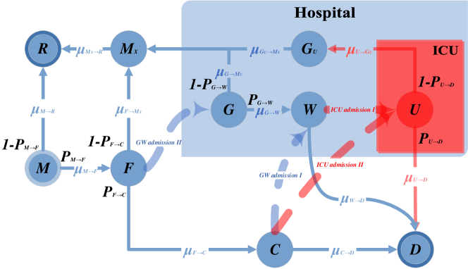
Supplementary Figure S1: Schematic diagram of the proposed COVID-19 patient admission model under limited medical resources. Each node represents a possible state of the patients. The specific definition of each state and the transition paths among them (light blue and light red arrows with time representing the average delay of the transition) are described in detail in the text. The various quantities $P_{\cdot\rightarrow\cdot}$ denote the fractions of the state transition paths, and the time delays follow a normal distribution. The light red dotted arrows indicate the two admission paths of ICU, where ICU admission I and II have the first and second priority, respectively. The light blue dotted arrows indicate the two treatment paths of GW, which have a lower priority than ICU admission: GW admission I and II have the third and fourth priority, respectively.

Our COVID-19 patient admission model under limited medical resources has ten dynamical states, as shown in Fig. S1. It describes the basic transition process of a diagnosed individual’s state from onset to recovery or death. Time delays associated with the various state transitions are taken into account, rendering non-Markovian the dynamical evolution. In particular, state M denotes that a patient is infected with COVID-19, state F means that the patient needs to be hospitalized but is currently under home isolation or centralized isolation, state C describes that the patient needs ICU support treatment but is currently isolated, states G and U indicate an inpatient occupying a GW and an ICU bed, respectively, a patient in state W currently occupies a GW bed but needs ICU treatment, a patient in the $G_{U}$ state is transferred out of ICU who does not need to occupy a GW bed, a patient in the $M_{x}$ state is discharged from the hospital with lessened symptoms, and the R and D states represent two clinical outcomes: recovery and death.

The medical resources can be divided into two categories: GW and ICU resources denoted as $Q_{G}$ and $Q_{U}$, respectively, which can be measured, e.g., by the corresponding numbers of beds. That the resources are limited is modeled, as follows. when the GW beds are all used up, new patients will no longer be admitted. When all ICU beds have been occupied, patients who require ICU care either continue to wait at GW (W-state) or continue to wait outside the hospital (C-state). A common hospital admission policy is “first-come first-serve” (FCFS), which gives priority to patients who have had a long waiting time. The admission policies of GW and ICU thus consist of four admission paths with different priorities: GW admission I/II and ICU admission I/II, where ICU admission I for W-state patients has the highest priority, followed by ICU admission II for C-state patients, GW admission I for the remaining C-state patients in GW, and GW admission II for the F-state patients. The priorities define the execution order of the corresponding paths. For M-state patients, two different transitions can occur: some patients deteriorating into the F-state so as to require hospitalization and others slowly recovering into the R-state. For patients in the F-state, there are three types of transitions: (i) when the GW resources are available, the patients are admitted to the hospital through GW admission II, (ii) a proportion of the remaining F-state patients deteriorate to C-state, requiring ICU treatment, and (iii) the rest are cured so they switch to the $M_{X}$-state. Patients in state C enter ICU through ICU admission II to transition into U-state, or through GW admission I to enter GW to become W-state, while the rest are in D-state. For G-state patients, some switch to $M_{X}$-state and no longer occupy GW resources, while others deteriorate to the W state, requiring ICU care. W-state patients will enter ICU through ICU admission I, and the remaining will be in the D state. Some of the U-state patients occupying ICU resources will transition to the $G_{U}$ state, and the others will switch to the D state. For patients in the $G_{U}$ state, the symptoms are relieved after a period time and they enter the $M_{X}$ state. Patients in the $M_{X}$ state recover to the R state after a period of time.

Let $\bigtriangleup Q_{G}$ and $\bigtriangleup Q_{U}$ denote the changes in the GW and ICU resources, respectively. A decrease in the GW resources is the sum of the number of patients admitted through the GW admission I/II pathway, and an increase is the sum of the number of ICU admission I, the number of patients in G (W)-state cured (or died), and the amount of newly deployed GW resources. Likewise, a decrease in ICU resources is the sum of the number of patients admitted through ICU admission I/II pathway, and an increase is the sum of the number of patients cured (or died) in state U and any newly deployed ICU resources. The state dynamical evolution described by a set of difference equations with time delays characterizing the state ages [Supplementary Note 1 (SN 1)].

Results

We validate our ten-state model by simulating the trend of the death tolls in Wuhan and Lombardy, using the daily number of confirmed cases, clinical and demographic data. The model then enables us to assess the overall effects of varying the timing of resource deployment and its amount on the COVID-19 mortalities. At a more detailed level, we divide the patients into several age groups and calculate the death-toll trend in each age group. This allows us to assess the impact of resource allocation scheme of different age groups on the number of deaths, and to obtain the optimal ICU admission strategy in terms of the age structure and outbreak scale with limited medical resources.

Impact of limited medical resource deployment

Model validation

To simulate the trend of the death tolls in Wuhan and Lombardy using the the second-order difference equations in our modeling framework, three types of data are required: time delays associated with state transitions, patient morbidity data, and local medical resource deployment data. The details of these data are described in SN2 and Supplementary tables S1-S5. which include information such as the average number of days in the transition delay from M-state to F-state and the average mortality rate of patients in ICU. Most of the data were obtained through references and official reports [17, 18, 19]. As detailed in SN2, the values of some model parameters need to be estimated in an optimal way, e.g., at the 95% confidence level, through model simulation and empirical data such as the average fraction of the patients switching from G-state to W-state, denoted as $|P|_{G\rightarrow W}$, and that from F-state to C-state, denoted as $|P|_{F\rightarrow C}$. We use the cumulative days of insufficient GW and ICU resources to quantify the level of stress on the healthcare system, defined as the GW overload days $O_{G}$ and ICU overload days $O_{U}$ (see SN3 - medical system stress level indicators).

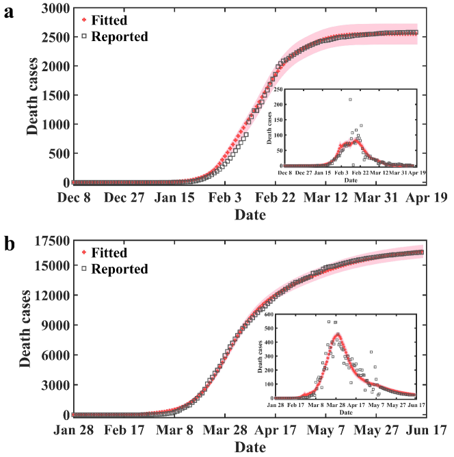
Supplementary Figure S2: Simulation results of the daily evolution of death tolls for the two COVID-19 epicenters. (a,b) Actual data of cumulative death toll with time in Wuhan and Lombardy, respectively. The insets show the daily numbers of new deaths. The open black squares and red crosses represent the actual data and simulation results, respectively. The pink shaded area marks the 95% confidence interval. There is a good agreement between the simulated daily number of deaths and the actual data, validating our ten-state model.

With the optimal parameter values and empirical data as inputs to the model, we simulate the cumulative death toll and new deaths over time in Wuhan (from December 8, 2019 to April 15, 2020) and Lombardy (from January 28 to June 14, 2020), as shown in Fig. S2. It can be seen that the model predicted trends of the cumulative and daily new death tolls agree with the actual data very well, validating the model. The model also gives that the values of $O_{G}$ are 14 and 17 days for Wuhan and Lombardy, respectively, and the corresponding values of $O_{U}$ are 49 and 74 days.

Deployment of medical resources

Since the onset of COVID-19 pandemic, many countries (most notably the USA) and regions have missed the best time window to control the spreading. At the present, there is a skyrocketing increase in the demand for ICU beds and medical resources such as ventilators and other special medical devices. Many hospitals and healthcare facilities have reached or will soon reach the limit of their operating capacities.

Optimizing the usage of medical resources by deploying them as early as possible and augmenting them as much as possible are key to reducing the mortality rate. Let DT and RI denote the two key parameters: the deployment time and the resource input, where $\mbox{DT}=0$ and $\mbox{RI}=1$ represent the actual deployment time and the available normalized amount of resources, respectively. If the resources are deployed seven days ahead of the actual time, we have $\mbox{DT}=-7$. Likewise, if the resources are doubled (e.g., twice as many ICU beds as in the actual case), we have $\mbox{RI}=2$ (see SN3 for COVID-19 special medical resource deployment plans). A virtue of our modeling framework lies in its ability to provide a quantitative picture of the dependence of the mortalities on the two key parameters.

To uncover the impact of deploying medical resources on the patient mortality rate in a concrete way, we consider the following three scenarios: (i) varying the GW resources only, (ii) varying ICU resources only, and (iii) varying both resources simultaneously. Some representative results are presented below (more results in SN4).

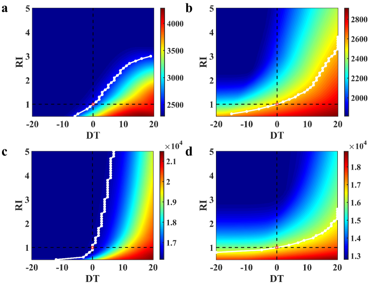
Supplementary Figure S3: Impact of timing of medical resource deployment and resource input on COVID-19 mortalities. Each panel shows the number of deaths (color coded) in the parameter plane of deployment time and resource input: panels (a,b) are for Wuhan, China, and (c,d) are for Lombardy region, Italy. In panels (a,c), the ICU resource amount is fixed and the resource that varies is GW. In panels (b,d), the GW resource amount is fixed and the resources that vary are ICU. The red hexagon indicates the true death toll under the actual resource deployment, and the white circles mark the contour of the actual death toll in the parameter plane.

Figure S3(a) shows, for Wuhan, the impact of varying GW resource deployment on the number of deaths for fixed ICU resource deployment, where the red hexagon indicates the true death toll under the actual resource deployment. If the GW resources had been deployed one week in advance or if its amount had been doubled, the death toll would have been reduced by 10%. While remarkable, this 10% figure is about the maximum reduction that can be achieved by varying the GW resource deployment. For example, deploying the GW resources earlier than one week or an increase in its investment over three times would not reduce the death toll further. The maximum reduction in the deaths that can be achieved is determined approximately by the contour of the actual death toll - the curve connecting the white circles Fig. S3(a). These results indicate that deploying the GW resources earlier and/or augmenting them have only limited effects on reducing the deaths.

In contrast, deploying the ICU resources earlier and/or augmenting them can be more effective at reducing the deaths in Wuhan, as shown in Fig. S3(b), where the GW resource deployment is fixed. If the ICU resources had been deployed one week ahead of the actual time or if the ICU resource amount had been doubled, the death toll would have been decreased by 5% and 13% respectively. While these figures are similar to those that would have been achieved with the same adjustment in the GW resources [Fig. S3(a)], deploying the ICU beds earlier or increasing their number can have a much more significant effect on the number of deaths. For example, if the number of ICU beds had been tripled, the death toll would have been reduced by 21%! The maximum reduction in the deaths is achieved for $\mbox{DT}=-14$ and $\mbox{RI}=2.5$, which is about 30% (about three times more effective than that which can be achieved by stretching the GW resources and their deployment). The corresponding ICU overload days would have been decreased to less than seven days (comparing with the actual 49 days for Wuhan). Similar results are obtained for Lombardy. We find that adjusting the GW resource deployment would have only limited effects in reducing the death toll. For example, as shown in Fig. S3(c), if the GW resources had been deployed one week or two weeks earlier or if the number of GW beds had been doubled or tripled, the reduction in the deaths would have been only about 1%. This indicates that the deployment of the GW resources in Lombardy was timely and its amount was appropriate, a fact that can also be seen from the value of the GW overload days $O_{G}$: to make it less than a week, the resources would need to be deployed only five days earlier or the number of GW beds would need to be only 1.4 times higher. In contrast, deploying the ICU resources earlier or augmenting them would have been much more effective at r educing the deaths. For example, if the number of ICU beds had been tripled, the death toll would have been reduced by 21%, as shown in Fig. S3(d). The maximum reduction that can be achieved is about 22% and $O_{U}$ can be decreased to less than a week.

SN3 presents results on the impact of varying the GW and ICU resource deployment simultaneously on COVID-19 death toll for both Wuhan and Lombardy.

Admission strategy based on age groups

To improve the efficiency of treatment and to reduce the mortality rate, it is essential and imperative to allocate the available resources as reasonably as possible because as they are not unlimited. For COVID-19, the hospitalization and mortality rates of elderly patients are higher than those of younger patients [20]. A common strategy is to divide the patients into distinct age groups. Our modeling framework provides a rigorous way to calculate the mortalities for different age groups.

Age groups

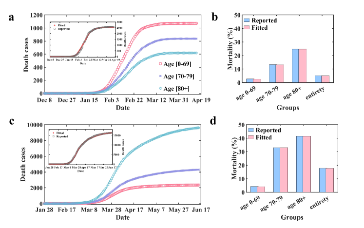
Supplementary Figure S4: Evolution of death toll with time for different age groups. (a) Simulated evolution trend of the death toll of the three age groups in Wuhan; (b) the actual mortality rate of each age group in Wuhan in comparison with model prediction; (c,d) the corresponding results for Lombardy. The insets in (a) and (c) display the actual daily death toll and model predictions for Wuhan and Lombardy, respectively. In panels (b) and (d), the light blue and pink columns represent the actual and simulated mortality rate of each group, respectively.

Individuals in any age group have the possibility of getting infected by COVID-19 with certain death risk [21]. Currently available data indicate that, in most countries, the risk of hospitalization and death increases with age [22, 23]. A direct manifestation is that the fraction of hospitalized patients and ICU mortality vary among the age groups.

For Wuhan, the available data divide patients into three groups: [0-69] years old, [70-79] years old, and [80+] years old. A similar division scheme applies to Lombardy. We use a linear regression to obtain the estimates of the fractions of various state transitions for each age group: $P_{M\rightarrow F}$, $P_{G\rightarrow W}$, $P_{F\rightarrow C}$ and $P_{U\rightarrow D}$. (SN4 provides more details.)

We input the parameters associated with each age group into the model and calculate the death tolls as a function of time for Wuhan and Lombardy. Figure S4 shows that the mortalities obtained from the simulation agree well with those of the actual data. Figures S4(a) and S4(c) show that the death toll of patients over 80 years old in Wuhan is the lowest among the age groups, while it is the highest in Lombardy: about 59%. There are two possible reasons for this difference. First, the aging populations in the two regions are different: the fraction of people over 65 years old is 14.06% in Wuhan and 20% in Lombardy [24, 25]. The elderly have weak autoimmunity and most of them have preexisting, underlying diseases, resulting in an excessively high death rate in Lombardy. The second reason is that more extensive tests were conducted in China (near 100%), enabling more young people with mild symptoms to be detected and included in the statistics. In contrast, as of April 29, 2020, there were about 1910761 people in Italy who had been tested, of whom 203591 were diagnosed with COVID-19 - about 11% only [26]. Nonetheless, Figs. S4(b) and S4(d) show that the mortality rate of patients over 70 years old is higher than that of patients under 70 for both Wuhan and Lombardy. Especially, in Lombardy, the mortality rate of patients over 80 years old reached 41%.

When the population is divided into nine age groups, our model generates essentially the same phenomenon that the risk of death increases with age (SN5).

Group weighting strategy

People of all ages have certain risk of being infected with COVID-19. Setting priority of admission for certain age groups can reduce the number of deaths. In Wuhan, the ICU resources were more scarce than GW resources, so making ICU admission policy dependent on age is especially important for suppressing the mortality rate. That is, the conventional FCFS admission policy is not suitable for COVID-19 under limited ICU resources. To set the priority of admission for different age groups, we shift the state age of each group by a priority weight. We then change the admission order of different age groups with the goal to find an optimal set of weights that minimizes the number of deaths. In particular, we set the priority weight of the $i_{th}$ age group as $w_{i}$ and record $\tau_{i}$ as the state age of the this age group. After weighting, the new state age $\tau_{i}^{{}^{\prime}}$ becomes,

$$\tau_{i}^{{}^{\prime}}=\tau_{i}+w_{i}.$$ (1)

The state age of patients in the $i_{th}$ age group is increased by $w_{i}$ days. The patients, after incorporating the weighted state age, are admitted according to FCFS.

To carry out the optimization procedure, we fix the priority weight of the second age group, i.e., the [70, 80) age group, to be $w_{2}=30$. As the state age of each group does not exceed 15, we implement different admission strategies for the age groups by changing the value of $w_{1}$ and $w_{3}$ (see SN5 for a specific method).

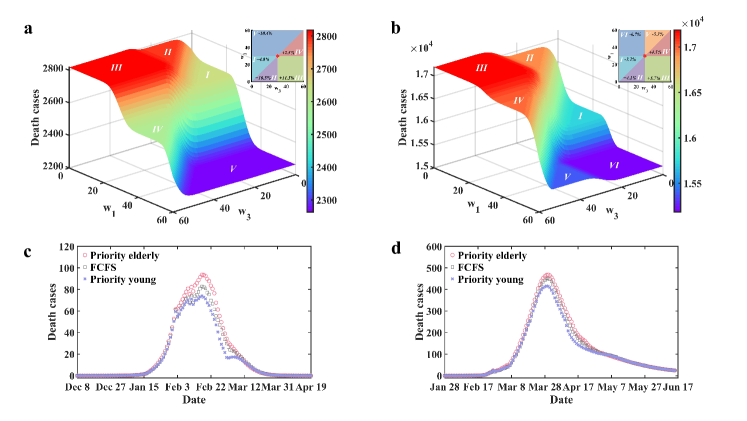
Supplementary Figure S5: Dependence of death toll on weights. (a,b) Model generated death toll and its dependence on $w_{1}$ and $w_{3}$ for fixed $w_{2}=30$ for Wuhan and Lombardy, respectively, where the blue and purple colors correspond to relatively fewer deaths. In the regions marked by Roman numerals, the death toll changes slowly with weights. The insets show the distribution of the number of deaths for different weight combinations, where the numerical values represent the differences in the number of deaths than that from the FCFS treatment strategy. (c,d) Daily number of new deaths under different admission strategies for Wuhan and Lombardy, respectively, where red circles, gray boxes, and blue-purple forks denote the results from the three strategies: preferential treatment for elderly patients, FCFS, and preference for young patients, respectively. Giving priority to young patients results in the lowest daily death curve.

Figure S5 shows the effect of the state age of groups 1 and 3 on the number of deaths when the weight of group 2 is fixed at constant (30). The larger the state age, the higher priority of admission is. When adjusting the weights of the first and third groups, their correspond state ages will vary and so the admission order of each age group will change accordingly. Different orders of treatment will lead to different death tolls. Figure S5 reveals, in the parameter plane of $(w_{1},w_{3})$, five distinct death toll regions for Wuhan. For Lombardy, there are six such regions, as shown in Fig. S5(b). The weight range in region V in Fig. S5(a) corresponds to the ranges in regions V and VI in Fig. S5(b), due to the relatively small fraction of patients in the third group in Wuhan. When patients in the first group are given the priority, the treatment order of the patients in the third group has little impact on the total number of deaths. While the patients in the third group in Lombardy have a large proportion, giving the priority to the first group will have a significant impact. In this case, the order of treatment for patients in the third group will affect the total number of deaths.

In Fig. S5, the number of deaths in Wuhan and Lombardy in parameter region I increases by 4.8% and decreases by 3.2%, respectively, in comparison with the death tolls from the FCFS treatment strategy, for $w_{2}>w_{1}>w_{3}$. Area II in Fig. S5 shows the number of deaths for $w_{2}>w_{3}>w_{1}$. Comparing with the FCFS strategy, the number of deaths increases by 10.5% and 4.1% for Wuhan and Lombardy, respectively. In area III in Fig. S5, the weighting order is $w_{3}>w_{2}>w_{1}$ and the largest death tolls are observed in Wuhan and Lombardy, as characterized by an increase of 11% and 5.7%, respectively, in comparison with the FCFS case. In area IV in Fig. S5 where the order of priority is $w_{3}>w_{1}>w_{2}$, the death tolls in Wuhan and Lombardy increase by 2.5% and 4.5%, respectively. In area V in Fig. S5(a), we have $w_{1}>w_{3}>w_{2}$, and the number of deaths in Wuhan is the lowest as represented by a decrease of 10.4% relative to that associated with the FCFS strategy. In the same area V for Lombardy, the corresponding decrease in the death toll is by 5.3%, as shown in Fig. S5(b). In area VI in Fig. S5(b), the priority ordering is $w_{1}>w_{2}>w_{3}$ and there is a decrease of 6.7% in the death toll. The implication of these results is that giving the treatment priority to young patients will reduce the number of deaths but giving priority to elderly patients will increase the death toll. Due to the resource limit, this strategy is intuitively reasonable and has in fact been commonly practiced in many hospitals and healthcare facilities. Our results provide a validation at a quantitative level.

Figures S5(c) and S5(d) demonstrate the evolution of new deaths over time in Wuhan and Lombardy, respectively, under different admission strategies. In both cases, there is no significant difference in the number of deaths in the early stages of the epidemic under three treatment strategies. When the epidemic has lasted for a period of time and the death toll increases sharply, giving priority to young patients can significantly reduce the number of deaths. At the end of the epidemic, again the differences among the three treatment strategies diminish. Taken together, these results verify that, under limited medical resources, during the rapidly increasing phase of COVID-19 infection, admitting and treating young patients are necessary to reduce the final death toll.

Optimization efficiency

When the ICU resources are in a serious shortage, medical staff have to face the hard choice of adopting the strategy of giving priority to treating young patients with a higher survival probability. The strategy’s effectiveness notwithstanding, it has serious implications for medical ethics. It is thus worth evaluating this admission/treatment strategy further. To this end, we exploit our model to study more extensively the impacts of different strategies for four countries: China, South Korea, Italy, and Spain. For each country, we collect information about the numbers of GW and ICU beds per 100000 population and about the age distribution of patients diagnosed with COVID-19. For example, in China and Italy, the numbers of ICU beds per 100000 individuals are 3.6 and 12.5, respectively. (A detailed display of the information can be found in SN6). We define the time-dependent optimization efficiency as

$$E(t)=\frac{V_{Q}(t)}{V_{Y}(t)},$$ (2)

where $V_{Q}(t)$ and $V_{Y}(t)$, respectively, are the numbers of new deaths per day with the FCFS and the age-selective strategy. In the asymptotic time limit $t\rightarrow\infty$ when the system has reached a steady state, $E(\infty)$ characterizes the final optimization efficiency. Since information about the average state transition fractions for patients in all four countries is not available, we use the model parameter values for Wuhan and Lombard to calculate the value of $E(\infty)$ for four countries versus the average daily patient size.

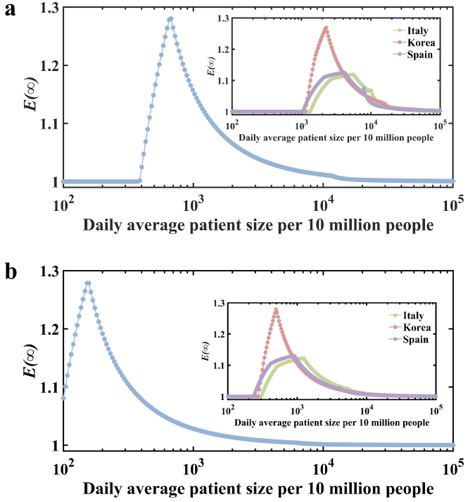
Supplementary Figure S6: Asymptotic optimization efficiency in China, Korea, Italy, and Spain. Shown is the steady-state efficiency $E(\infty)$ versus the cases per ten million people. (a) The result for China based on the parameter values from Wuhan. Inset shows the corresponding results for Italy, South Korea, and Spain. (b) The result for China based on the parameter values from Lombardy and the results for the other three countries are displayed in inset.

Based on the per capita medical resource data of the four countries as well as the age distribution data of confirmed patients in each country, making use of the relevant model parameter values for Wuhan and Lombard, we calculate $E(\infty)$ of the four countries versus the daily average patient size. We assume that up to 50% of the medical resources can be deployed to treating patients with COVID-19. As shown in Fig. S6, when the number of patients is below 100, the value of $E(\infty)$ for the four countries is equal to one. In this case, there is no need to implement the age-selective admission strategy. When the number of patients exceeds a critical value, $E(\infty)$ for all four countries increases rapidly as the number of patients increases through the critical value and then reaches a peak value. In fact, for a wide range of variation of the patient size, the values of $E(\infty)$ are high. Note that the peak values of $E(\infty)$ for China and South Korea are slightly below 1.3, but those for Italy and Spain are lower than 1.2 with a relatively slow increasing rate to reach the peak value. A plausible reason lies in the difference in the age distribution of patients diagnosed with COVID-19 in the eastern and western countries. In particular, in China and South Korea, less than 12% of the patients are over 70 years old, while those in Italy and Spain account for 37% and 34%, respectively (SN6). The value of $E(\infty)$ is highly correlated with the availability of the ICU beds. For $E(\infty)=1$, ICU beds are fully sufficient, but $E(\infty)>1$ signifies a shortage of ICU beds. Figure S6(a) reveals that, with the per capita medical resources of South Korea, Italy, and Spain, the need for ICU of 1,000 cases per tens of millions of people per day can be met for a long time, while the capacity of China may be less than half of the capacity of those countries. Indeed, the number of ICU beds per capita in China is 3.6 per 100000 persons, while the corresponding numbers in Italy, South Korea, and Spain are 12.5, 10.6, and 9.7, respectively (SN 6). We conclude that, while the age-selective admission strategy is more effective in countries with a younger population structure, countries with less per capita ICU medical resources need to implement this strategy, particularly in the early stage of the pandemic when the number of patients is relatively small.

Discussion

With the resurgence of COVID-19 cases in many countries and regions, a severe shortage of medical resources for treating the disease is inevitable, potentially leading to a significant death toll. To study the impact of limited medical resources on the patient mortality at a quantitative level can provide insights into developing optimal resource allocation schemes to reduce the number of deaths. Based on the COVID-19 data, medical resources and other relevant information, we have developed an admission treatment model subject to limited medical resources, which enables a quantitative and systematic assessment of the mortality rate associated with various resource allocation scenarios. Using empirical data from Wuhan and Lombardy, we validate the model by demonstrating that it can reproduce accurately the evolution of daily death toll in both places. The validated model is then used to assess the impact of different scenarios of medical deployment (including deployment time and resource investment) on the number of deaths. In general, the ICU resources have a significant impact on the mortality rate, and it is intuitively evident that deploying the ICU resources earlier and/or augmenting them will reduce the death toll. A virtue of our model is that it enables an accurate quantification of such intuitive expectations. For example, we find that, if the deployment of ICU resources had been made one week earlier or if they had been doubled, the death toll in Wuhan would have been reduced by 5% or 13%, and that in Lombardy by 3% and 14%, respectively. If the number of ICU beds had been tripled, the death toll in both Wuhan and Lombardy would have been reduced by 21%.

Our model enables an accurate prediction of the COVID-19 death toll for any combination of the two parameters: the amount of advance or delay in the timing of ICU deployment and the enhancement factor of the ICU resources. Our model asserts that simultaneously advancing the timing of ICU resource deployment and enhancing the ICU resources will reduce the death toll significantly. For example, if the ICU resources had been augmented by a factor of 2.5 and deployed two weeks earlier than the actual date, the final death toll would have been reduced by 29% in Wuhan. In Lombardy, if the number of ICU beds had been three times the actual number and they had been placed into service one week earlier, the final death toll would have been reduced by 22% and the ICU ward overload days would have been suppressed to less than one week.

Likewise, our model is fully capable of assessing the impacts of GW resources on COVID-19 mortalities. For example, if the GW resources in Wuhan had been deployed one week in advance or if the GW resources had been doubled, the death toll would have been reduced by 10% comparing with the actual toll. However, the model predicts that deploying GW resources earlier than one week or augmenting them further would have little effect on suppressing the death toll further. For Lombardy, the GW resources play an even less role in reducing the death toll: augmenting them or deploying them earlier would reduce the death toll by about 1% at maximum. This indicates that the GW resources in Lombardy were sufficient. This should be contrasted with the scenario of significantly enhancing the ICU resources, e.g., by a factor of four, where the death toll would be reduced by 26% and 22% for Wuhan and Lombardy, respectively. The implication is that, in comparison with the GW resources, the actual ICU resources in Wuhan and Lombardy were far from sufficient.

The morbidity and mortality of patients infected with COVID-19 increase with age. We have studied the role of age selective admission and treatment strategies in the death toll. In general, giving admission priorities to patients in different age groups would result in different mortality rate. In particular, if priorities had been given to the younger age groups, the number of deaths in Wuhan and Lombardy would have been reduced by 10.4% and 6.7%, respectively, in comparison with that from the normal FCFS strategy. In contrast, if priority had been given to elderly patients, the number of deaths would have increased by 11.5% and 5.7% for the two places, respectively.

The optimal admission/treatment strategies also depend on the scale of COVID-19 outbreak, the age structure of patients in the general population, and the per capita medical resources. We have quantified these effects by defining the steady-state optimization efficiency $E(\infty)$ and calculated this quantity for four countries: China, South Korea, Italy, and Spain. One finding is that, when the number of patients exceeds a threshold value, the values of $E(\infty)$ for the four countries first rise rapidly with the increase of the epidemic scale and then reaches a peak value. Remarkably, $E(\infty)$ can be maintained at a high value in a wide range of the epidemic scale. The peak values of Italy and Spain are both lower than 1.2, and the rising rate is slower. However, the peak values of China and South Korea are both close to 1.3. This discrepancy between the two eastern Asian and two western countries can be explained by the age distribution of the patients diagnosed with COVID-19: in China and South Korea, less than 12% of the diagnosed patients are over 70 years old, while those in Italy and Spain account for about 35%. The per capita medical resources of South Korea, Italy and Spain can meet the long term demand of 1000 cases per tens of million people per day, while the caring capacity of China may be less than half of that of the these countries. This is due to the small number of ICU beds per capita in China, which is 3.6 per 100000 persons, compared with 12.5, 10.6, and 9.7 in Italy, South Korea, and Spain, respectively. We conclude that the age-selective admission strategy is more effective in countries with a younger age structure, while the countries with less per capita ICU medical resources may need to implement this admission strategy in the early stage of the epidemic when the number of patients is relatively small.

Our model provides a general evaluation framework for assessing, at a quantitative level, the necessary medical resource deployment and admission strategy. It can be used to predict and articulate, under limited medical resources, optimal scenarios with respect to resource deployment and hospital admission/treatment strategies to minimize the death toll for future outbreaks of infectious diseases.

Data Availability

All relevant data are available from the authors upon request.

Code Availability

All relevant computer codes are available from the authors upon request.

Author Contributions

M.T. designed research; Y.-Q.Z., L.Z. performed research; Y.-Q.Z., L.Z., M.T., Y.L., Z.L., and Y.-C.L. analyzed data; Y.-Q.Z., L.Z., M.T., Z.L., and Y.-C.L. wrote the paper.

Competing Interests

The authors declare no competing interests.

Correspondence

To whom correspondence should be addressed. E-mail: tangminghan007@gmail.com; Ying-Cheng.Lai@asu.edu

Supplementary Information for

Quantitative assessment of the effects of resource optimization and ICU admission policy on COVID-19 mortalities

Ying-Qi Zeng, Lang Zeng, Ming Tang^∗, Ying Liu, Zong-Hua Liu, and Ying-Cheng Lai^∗

Supplementary Note 1: Equations governing non-Markovian dynamical evolution of states

Because of the non-Markovian nature of the dynamical evolution of the states, it is convenient to describe the underlying process in terms of difference equations over infinitesimal intervals in both time delay and time. In the following, we derive, one by one, the difference equations for all the ten states in our model.

M state

The evolution equation of the number of M-state patients with state age $\tau$ at time $t$ is

$$M(\tau+d\tau;t+dt) =[1-{\omega_{M\rightarrow F}}(\tau)d\tau]\frac{{{P_{M\rightarrow F}}\int_{\tau}^{+\infty}{{f_{M\rightarrow F}}(\tau^{{}^{\prime}})}d\tau^{{}^{\prime}}}}{{{P_{M\rightarrow F}}\int_{\tau}^{+\infty}{{f_{M\rightarrow F}}(\tau^{{}^{\prime}})}d\tau^{{}^{\prime}}+(1-{P_{M\rightarrow F}})\int_{\tau}^{+\infty}{{f_{M\rightarrow R}}(\tau^{{}^{\prime}})}d\tau^{{}^{\prime}}}}M(\tau;t)$$ (3)

$$+[1-{\omega_{M\rightarrow R}}(\tau)d\tau]\frac{{(1-{P_{M\rightarrow F}})\int_{\tau}^{+\infty}{{f_{M\rightarrow R}}(\tau^{{}^{\prime}})}d\tau^{{}^{\prime}}}}{{{P_{M\rightarrow F}}\int_{\tau}^{+\infty}{{f_{M\rightarrow F}}(\tau^{{}^{\prime}})}d\tau^{{}^{\prime}}+(1-{P_{M\rightarrow F}})\int_{\tau}^{+\infty}{{f_{M\rightarrow R}}(\tau^{{}^{\prime}})}d\tau^{{}^{\prime}}}}M(\tau;t),$$

where $M(\tau;t)$ is the density function of M-state patients with state age $\tau$ at time $t$, so the number of nodes in the M state with the state age in the interval $(\tau,\tau+d\tau)$ is $M(\tau;t)d\tau$. A node in the M state enters the F state (R state) at the conditional rate $\omega_{M\to F}(\tau)$ [$\omega_{M\to R}(\tau)$], which are given by

$$\omega_{M\to F}(\tau) = \frac{f_{M\to F}(\tau)}{\int_{\tau}^{+\infty}f_{M\to F}(\tau^{\prime})d\tau^{\prime}},$$

$$\omega_{M\to R}(\tau) = \frac{f_{M\to R}(\tau)}{\int_{\tau}^{+\infty}f_{M\to R}(\tau^{\prime})d\tau^{\prime}},$$

where $f_{M\rightarrow F}(\tau)$ and $f_{M\rightarrow R}(\tau)$ are the probability density functions of the time delay from the M state to the F and R states, respectively, each representing the probability of a state transition within the time interval $(t,t+dt)$. Since the M state can transition to two different states: $M\rightarrow F$ and $M\rightarrow R$, the two processes will compete with each other, so the remaining probabilities of the state transitions at time $t$ are

$$\frac{{{P_{M\rightarrow F}}\int_{\tau}^{+\infty}{{f_{M\rightarrow F}}(\tau^{{}^{\prime}})}d\tau^{{}^{\prime}}}}{{{P_{M\rightarrow F}}\int_{\tau}^{+\infty}{{f_{M\rightarrow F}}(\tau^{{}^{\prime}})}d\tau^{{}^{\prime}}+(1-{P_{M\rightarrow F}})\int_{\tau}^{+\infty}{{f_{M\rightarrow R}}(\tau^{{}^{\prime}})}d\tau^{{}^{\prime}}}},$$ (4)

and

$$\frac{{(1-{P_{M\rightarrow F}})\int_{\tau}^{+\infty}{{f_{M\rightarrow R}}(\tau^{{}^{\prime}})}d\tau^{{}^{\prime}}}}{{{P_{M\rightarrow F}}\int_{\tau}^{+\infty}{{f_{M\rightarrow F}}(\tau^{{}^{\prime}})}d\tau^{{}^{\prime}}+(1-{P_{M\rightarrow F}})\int_{\tau}^{+\infty}{{f_{M\rightarrow R}}(\tau^{{}^{\prime}})}d\tau^{{}^{\prime}}}},$$ (5)

respectively.

The newly increased patients enter the M state. Suppose that $Z_{M}(t)$ new patients are added within $(t,t+dt)$, we have

$$M(0;t+dt)=Z_{M}(t).$$ (6)

The state age of the newly added M-state patients is zero.

F state

The evolution equation of the number of F-state patients with state age $\tau$ at time $t$ is

$$F(\tau+d\tau;t+dt) =[1-{\omega_{F\rightarrow C}}(\tau)d\tau]\frac{{{P_{F\rightarrow C}}\int_{\tau}^{+\infty}{{f_{F\rightarrow C}}(\tau^{{}^{\prime}})}d\tau^{{}^{\prime}}}}{{{P_{F\rightarrow C}}\int_{\tau}^{+\infty}{{f_{F\rightarrow C}}(\tau^{{}^{\prime}})}d\tau^{{}^{\prime}}+(1-{P_{F\rightarrow C}})\int_{\tau}^{+\infty}{{f_{F\rightarrow M_{X}}}(\tau^{{}^{\prime}})}d\tau^{{}^{\prime}}}}F(\tau;t)$$ (7)

$$+[1-{\omega_{F\rightarrow M_{X}}}(\tau)d\tau]\frac{{{(1-P_{F\rightarrow C})}\int_{\tau}^{+\infty}{{f_{F\rightarrow M_{X}}}(\tau^{{}^{\prime}})}d\tau^{{}^{\prime}}}}{{{P_{F\rightarrow C}}\int_{\tau}^{+\infty}{{f_{F\rightarrow C}}(\tau^{{}^{\prime}})}d\tau^{{}^{\prime}}+(1-{P_{F\rightarrow C}})\int_{\tau}^{+\infty}{{f_{F\rightarrow M_{X}}}(\tau^{{}^{\prime}})}d\tau^{{}^{\prime}}}}F(\tau;t),$$

with notations similar in their meanings to those of the M-state equation.

After admission of patients in the C state, the remaining available GW resources are $\Delta Q_{G}^{{}^{\prime}}(t)$. There are two cases: (i) the new resources available are sufficient to accommodate all F-state patients; (ii) new available resources can only accept some or none of the F-state patients. In these two cases, patients in the F state are admitted according to the strategy of FCFS (first-come first-serve). The number of F-state patients changing to the G state in $(t,t+dt)$ is denoted as $\bigtriangleup_{F\rightarrow G}(t)$.
In the first case where the GW resources are sufficient to accommodate all current F-states patients, if

$$\Delta Q_{G}^{{}^{\prime}}(t)(t)\geq\int_{0}^{+\infty}F(\tau+d\tau;t+dt)d\tau,$$

then all F-state individuals will change to the G state. We have $F(\tau+d\tau;t+dt)=0$ for all $\tau$ $\in$ [0,$+\infty$), and

$$\bigtriangleup_{F\rightarrow G}(t)=\int_{0}^{+\infty}F(\tau+d\tau;t+dt)d\tau.$$

In the second case where the GW resources can hold only some or none of the current F-state patients, if

$$\Delta Q_{G}^{{}^{\prime}}(t)(t)=\int_{\tau_{c}}^{+\infty}F(\tau+d\tau,t+dt)d\tau,$$

then some F-state individuals will change to the G state. We have $F(\tau+d\tau;t+dt)=0$ for $\tau$ $\in$ [$\tau_{c}$,$+\infty$), and

$$\bigtriangleup_{F\rightarrow G}(t)=\Delta Q_{G}^{{}^{\prime}}(t)(t).$$

When the patients in the M state enter into the F state, the initial state age is set to be zero. The number of newly added F-state patients is given by

$$F(0;t+dt)=\int_{0}^{+\infty}\omega_{M\to F}(\tau)\frac{P_{M\to F}\int_{\tau}^{+\infty}f_{M\to F}(\tau^{\prime})d\tau^{\prime}}{P_{M\to F}\int_{\tau}^{+\infty}f_{M\to F}(\tau^{\prime})d\tau^{\prime}+(1-P_{M\to F})\int_{\tau}^{+\infty}f_{M\to R}(\tau^{\prime})d\tau^{\prime}}M(\tau;t)d\tau.$$ (8)

C state

The evolution equation of the number of C-state patients with state age $\tau$ at time $t$ is

$$C(\tau+d\tau;t+dt)=[1-\omega_{C\to D}(\tau)d\tau]C(\tau;t).$$ (9)

To get the number of C-state patients admitted to the hospital, we note that there are two admission paths: (a) through ICU admission II to the U state; (b) through GW admission I to the W state.

ICU admission II path. After admission of W-state patients, the remaining available ICU resources are $\Delta Q_{U}^{\prime}(t)$. There are two cases: (i) the newly available resources are sufficient to accommodate all the C-states patients and (ii) the newly available resources are able to accommodate some or none of the C-state patients. The number of C-state patients who switch to the U state in $(t,t+dt)$ time interval is denoted as $\bigtriangleup_{C\rightarrow U}(t)$.

In case (i), if

$$\Delta Q_{U}^{\prime}(t)\geq\int_{0}^{+\infty}C(\tau+d\tau;t+dt)d\tau,$$

all C-state patients will change to the U state. We have $C(\tau+d\tau;t+dt)=0$ for $\tau\in$ [0,$+\infty$), and

$$\bigtriangleup_{C\rightarrow U}(t)=\int_{0}^{+\infty}C(\tau+d\tau;t+dt)d\tau.$$

In case (ii), if

$$\Delta Q_{U}^{\prime}(t)=\int_{\tau_{c}}^{+\infty}C(\tau+d\tau;t+dt)d\tau,$$

and $0\leq\tau_{c}\leq+\infty$, then the C-state individuals whose state ages are greater than $\tau_{c}$ will enter the U state. We have $C(\tau+d\tau,t+dt)=0$ for $\tau\in$ [$\tau_{c}$,$+\infty$) and

$$\bigtriangleup_{C\rightarrow U}(t)=\Delta Q_{U}^{\prime}(t).$$

The remaining C-state patients can switch to the W state through the GW admission I pathway.

GW admission I path. Considering that the remaining C-state patients are in critical conditions, when the ICU resources are unavailable to them, they will be admitted to GW and change into the W state with the highest priority. The available resources within the time interval $(t,t+dt)$ are denoted as $\Delta Q_{G}(t)$. There are two cases: (i) the available GW resources are enough to accommodate all the remaining C-state patients, and (ii) the available GW resources can accommodate some or none of the remaining C-state patients. The number of patients in the C state who change to the W state in $(t,t+dt)$ is denoted as $\bigtriangleup_{C\rightarrow W}(t)$.

In case (i), we have

$$\Delta Q_{G}(t)\geq\int_{0}^{+\infty}C(\tau+d\tau;t+dt)d\tau.$$

The amount of the remaining available resources through F-state patients for GW admission II is

$$\Delta Q^{\prime}_{G}(t)=\Delta Q_{G}(t)-\int_{0}^{+\infty}C(\tau+d\tau;t+dt)d\tau.$$

Individuals in the C state will change to the W state, so we have $C(\tau+d\tau;t+dt)=0$ for $\tau\in$ [0,$+\infty$), and

$$\bigtriangleup_{C\rightarrow W}(t)=\int_{0}^{+\infty}C(\tau+d\tau;t+dt)d\tau.$$

In case (ii), we have

$$\Delta Q_{G}(t)=\int_{\tau_{c}}^{+\infty}C(\tau+d\tau;t+dt)d\tau.$$

The amount of the remaining available resources for GW admission II is $\Delta Q^{\prime}_{G}(t)=0$. The C-state individuals with state ages greater than $\tau_{c}$ will enter the W state. We have $C(\tau+d\tau,t+dt)=0$ for $\tau\in$ [$\tau_{c}$,$+\infty$) and

$$\bigtriangleup_{C\rightarrow W}(t)=\Delta Q_{G}(t).$$

When the F-state patients enter the C state, the initial state age is set to be zero. The number of newly added C-state patients is

$$C(0;t+dt)=\int_{0}^{+\infty}\omega_{F\to C}(\tau)\frac{P_{F\to C}\int_{\tau}^{+\infty}f_{F\to C}(\tau)^{\prime}d\tau^{\prime}}{P_{F\to C}\int_{\tau}^{+\infty}f_{F\to C}(\tau)^{\prime}d\tau^{\prime}+[1-P_{F\to C}]\int_{\tau}^{+\infty}f_{F\to R}(\tau)^{\prime}d\tau^{\prime}}F(\tau;t)d\tau.$$ (10)

0.1 G state

The evolution equation of the number of G-state patients with state age $\tau$ at time $t$ is

$$G(\tau+d\tau;t+dt)=[1-\omega_{G\to W}(\tau)d\tau]\frac{P_{G\to W}\int_{\tau}^{+\infty}f_{G\to W}(\tau^{\prime})d\tau^{\prime}}{P_{G\to W}\int_{\tau}^{+\infty}f_{G\to W}(\tau^{\prime})d\tau^{\prime}+(1-P_{G\to W})\int_{\tau}^{+\infty}f_{G\to M_{X}}(\tau^{\prime})d\tau^{\prime}}G(\tau;t)$$ (11)

$$+[1-\omega_{G\to M_{X}}(\tau)d\tau]\frac{(1-P_{G\to W})\int_{\tau}^{+\infty}f_{G\to M_{X}}(\tau^{\prime})d\tau^{\prime}}{P_{G\to W}\int_{\tau}^{+\infty}f_{G\to W}(\tau^{\prime})d\tau^{\prime}+(1-P_{G\to W})\int_{\tau}^{+\infty}f_{G\to M_{X}}(\tau^{\prime})d\tau^{\prime}}G(\tau;t).$$

The number of newly added G-state patients is

$$G(0;t+dt)=\bigtriangleup_{F\rightarrow G}(t).$$ (12)

0.2 W state

The evolution equation of the number of W-state patients with state age $\tau$ at time $t$ is

$$W(\tau+d\tau;t+dt)=(1-\omega_{W\to D}(\tau)d\tau)W(\tau;t).$$ (13)

To have the number of W-state patients admitted to the hospital, we denote the available ICU resources at time $t$ as $\Delta Q_{U}(t)$. There are two cases: (i) there are sufficient resources to accommodate all current W-state patients, and (ii) the available resources can accommodate some or none of the W-state patients. The number of W-state patients who change to the U state in $(t,t+dt)$ is $\bigtriangleup_{W\rightarrow U}(t)$.

In case (i), if

$$\Delta Q_{U}(t)\geq\int_{0}^{+\infty}W(\tau+d\tau;t+dt)d\tau,$$

the amount of the remaining available resources is

$$\Delta Q^{\prime}_{U}(t)=\Delta Q_{U}(t)-\int_{0}^{+\infty}W(\tau+d\tau;t+dt)d\tau.$$

We have

$$W(\tau+d\tau;t+dt)=0\ for\ \tau\in[0,+\infty),\bigtriangleup_{W\rightarrow U}(t)=\int_{0}^{+\infty}W(\tau+d\tau;t+dt)d\tau.$$ (14)

In case (ii), if

$$\Delta Q_{U}(t)=\int_{\tau_{c}}^{+\infty}W(\tau+d\tau,t+dt)d\tau$$

and $0\leq\tau_{c}<+\infty$, the amount of the remaining available resources is $\Delta Q^{\prime}_{U}(t)=0$. We get

$$W(\tau+d\tau;t+dt)=0\ for\ \tau\in[\tau_{c},+\infty),\bigtriangleup_{W\rightarrow U}(t)=\Delta Q_{U}(t).$$ (15)

The sources of the W-state patients are the G-state patients whose conditions have deteriorated and the C-state patients admitted through GW admission I. The number of newly added W-state patients is

$$W(0;t+dt)=\bigtriangleup_{C\rightarrow W}(t)+\int_{0}^{+\infty}\omega_{G\to W}(\tau)\frac{P_{G\to W}\int_{\tau}^{\infty}f_{G\to W}(\tau^{\prime})d\tau^{\prime}}{P_{G\to W}\int_{\tau}^{\infty}f_{G\to W}(\tau^{\prime})d\tau^{\prime}+(1-P_{G\to W})\int_{\tau}^{\infty}f_{G\to M_{X}}(\tau^{\prime})d\tau^{\prime}}G(\tau;t)d\tau.$$ (16)

U state

The evolution equation of the number of U-state patients with state age $\tau$ at time $t$ is

$$U(\tau+d\tau;t+dt)=[1-\omega_{U\to D}(\tau)d\tau]\frac{P_{U\to D}\int_{\tau}^{+\infty}f_{U\to D}(\tau^{\prime})d\tau^{\prime}}{P_{U\to D}\int_{\tau}^{+\infty}f_{U\to D}(\tau^{\prime})d\tau^{\prime}+(1-P_{U\to D})\int_{\tau}^{+\infty}f_{U\to G_{U}}(\tau^{\prime})d\tau^{\prime}}U(\tau;t)$$ (17)

$$+[1-\omega_{U\to G_{U}}(\tau)d\tau]\frac{(1-P_{U\to D})\int_{\tau}^{+\infty}f_{U\to G_{U}}(\tau^{\prime})d\tau^{\prime}}{P_{U\to D}\int_{\tau}^{+\infty}f_{U\to D}(\tau^{\prime})d\tau^{\prime}+(1-P_{U\to D})\int_{\tau}^{+\infty}f_{U\to G_{U}}(\tau^{\prime})d\tau^{\prime}}U(\tau;t).$$

Patients in the U state are from the W state and the admitted C-state patients. The number of newly added U-state patients is

$$U(0;t+dt)=\bigtriangleup_{W\rightarrow U}(t)+\bigtriangleup_{C\rightarrow U}(t).$$ (18)

$G_{U}$ state

The evolution equation of the number of $G_{U}$-state patients with state age $\tau$ at time $t$ is

$$G_{U}(\tau+d\tau;t+dt)=[1-\omega_{G_{U}\to M_{X}}(\tau)d\tau]G_{U}(\tau;t).$$ (19)

The number of newly added $G_{U}$-state patients is

$$G_{U}(0;t+dt)=\int_{0}^{+\infty}\frac{(1-P_{U\to D})\omega_{U\rightarrow G_{U}}(\tau)\int_{\tau}^{+\infty}f_{U\to G_{U}}(\tau^{\prime})d\tau^{\prime}}{P_{U\to D}\int_{\tau}^{+\infty}f_{U\to D}(\tau^{\prime})d\tau^{\prime}+(1-P_{U\to D})\int_{\tau}^{+\infty}f_{U\to G_{U}}(\tau^{\prime})d\tau^{\prime}}U(\tau,t)d\tau.$$ (20)

$M_{X}$ state

The evolution equation of the number of $M_{X}$-state patients with state age $\tau$ at time $t$ is

$$M_{X}(\tau+d\tau;t+dt)=[1-\omega_{M_{X}\to R}(\tau)d\tau]M_{X}(\tau;t).$$ (21)

The sources of $M_{X}$ state patients are three: patients from the F, G, and $G_{U}$ states. The number of newly added $M_{X}$-state patients is given by

$$M_{X}(0,t+dt) =\int_{0}^{+\infty}\omega_{G_{U}\to M_{X}}(\tau)G_{U}(\tau;t)d\tau$$ (22)

$$+\int_{0}^{+\infty}\frac{(1-P_{G\to W})\int_{\tau}^{+\infty}f_{G\to M_{X}}(\tau^{\prime})d\tau^{\prime}}{P_{G\to W}\int_{\tau}^{+\infty}f_{G\to W}(\tau^{\prime})d\tau^{\prime}+(1-P_{G\to W})\int_{\tau}^{+\infty}f_{G\to M_{X}}(\tau^{\prime})d\tau^{\prime}}\omega_{G\to M_{X}}G(\tau;t)d\tau$$

$$+\int_{0}^{+\infty}\frac{(1-P_{F\to C})\int_{\tau}^{+\infty}f_{F\to M_{X}}(\tau^{\prime})d\tau^{\prime}}{P_{F\to C}\int_{\tau}^{+\infty}f_{F\to C}(\tau^{\prime})d\tau^{\prime}+(1-P_{F\to C})\int_{\tau}^{+\infty}f_{F\to M_{X}}(\tau^{\prime})d\tau^{\prime}}\omega_{F\to M_{X}}F(\tau;t)d\tau.$$

R state

The R-state patients come from the M and $M_{X}$ states. We have

$$R(t+dt) =R(t)+\int_{0}^{+\infty}\omega_{M_{X}\to R}M_{X}(\tau;t)d\tau$$ (23)

$$+\int_{0}^{+\infty}\frac{(1-P_{M\to F})\int_{\tau}^{+\infty}f_{M\to R}(\tau^{\prime})d\tau^{\prime}}{P_{M\to F}\int_{\tau}^{+\infty}f_{M\to F}(\tau^{\prime})d\tau^{\prime}+(1-P_{M\to F})\int_{\tau}^{+\infty}f_{M\to R}(\tau^{\prime})d\tau^{\prime}}\omega_{M\to R}M(\tau;t)d\tau.$$

D state

The D-state patients come from C, W, and U states. We have

$$D(t+dt) =D(t)+\int_{0}^{+\infty}\omega_{C\to D}C(\tau;t)d\tau+\int_{0}^{+\infty}\omega_{W\to D}W(\tau;t)d\tau$$ (24)

$$+\int_{0}^{+\infty}\frac{P_{U\to D}\int_{\tau}^{+\infty}f_{U\to D}(\tau^{\prime})d\tau^{\prime}}{P_{U\to D}\int_{\tau}^{+\infty}f_{U\to D}(\tau^{\prime})d\tau^{\prime}+(1-P_{U\to D})\int_{\tau}^{+\infty}f_{U\to G_{U}}(\tau^{\prime})d\tau^{\prime}}\omega_{U\to D}(\tau)U(\tau;t)d\tau.$$

Calculation of available ICU resources $\bigtriangleup Q_{U}(t)$

The available ICU resources are those that have been newly added, those that are released when patients go from the U state to the D state or the $G_{U}$-state patients, and the resources consumed by the W-state and C-state patients. We have

$$\Delta Q_{U}(t+dt) =\Delta Q_{U}(t)+Z_{U}(t)-\Delta_{W\rightarrow U}(t)-\Delta_{C\rightarrow U}(t)$$ (25)

$$+\int_{0}^{+\infty}\frac{P_{U\to D}\int_{\tau}^{+\infty}f_{U\to D}(\tau^{\prime})d\tau^{\prime}}{P_{U\to D}\int_{\tau}^{+\infty}f_{U\to D}(\tau^{\prime})d\tau^{\prime}+(1-P_{U\to D})\int_{\tau}^{+\infty}f_{U\to G_{U}}(\tau^{\prime})d\tau^{\prime}}\omega_{U\to D}(\tau)U(\tau;t)d\tau$$

$$+\int_{0}^{+\infty}\frac{(1-P_{U\to D})\int_{\tau}^{+\infty}f_{U\to G_{U}}(\tau^{\prime})d\tau^{\prime}}{P_{U\to D}\int_{\tau}^{+\infty}f_{U\to D}(\tau^{\prime})d\tau^{\prime}+(1-P_{U\to D})\int_{\tau}^{+\infty}f_{U\to G_{U}}(\tau^{\prime})d\tau^{\prime}}\omega_{U\to G_{U}}(\tau)U(\tau;t)d\tau.$$

Calculation of available GW resources $\Delta Q_{G}(t)$

The available GW resources are those that have been newly added, those released when patients switch from the G state to the $M_{x}$ state and from the W state to the D state or the U state, and the resources consumed by the C-state and F-state patients. We have

$$\Delta Q_{G}(t+dt) =\Delta Q_{G}(t)+Z_{G}(t)-\Delta_{C\rightarrow W}(t)-\Delta_{F\rightarrow G}(t)+\int_{0}^{+\infty}W(\tau;t)\omega_{W\to D}(\tau)d\tau$$ (26)

$$+\int_{0}^{+\infty}\frac{(1-P_{G\to W})\int_{\tau}^{+\infty}f_{G\to M_{X}}(\tau^{\prime})d\tau^{\prime}}{P_{G\to W}\int_{\tau}^{+\infty}f_{G\to W}(\tau^{\prime})d\tau^{\prime}+(1-P_{G\to W})\int_{\tau}^{+\infty}f_{G\to M_{X}}(\tau^{\prime})d\tau^{\prime}}\omega_{G\to M_{X}}(\tau)G(\tau;t)d\tau.$$

Supplementary Note 2: Parameter estimation

Average delay and fraction of state transition

As shown in Tab. S1, we assume that the time delay of patients switching from state M to F follows the normal distribution with the average of five days [17]. The distributions of the time delays associated with other state transitions are also assumed to be normal. The average time delays from the U state to the D and $G_{u}$ states are set as seven days [18, 19] and eight days [18], respectively, and that from the G state to the W state is three days [17]. In our model setting, the clinical symptoms of the F-state and G-state patients are identical, and the difference lies in whether the patients are admitted (i.e., occupying GW beds), and the same rule applies to the C-state and W-state patients.

The average time delay from the F to the C state is two days [17, 27], and that from the G and F states to the $M_{X}$ state is eight days [12]. The average time delays from the W and C states to the D state are assumed to be three days and one day, respectively.

As shown in Tab. S2, we set the average mortality rate of ICU patients as 61.5% [18, 28]. During the epidemic, due to the different testing methods and conditions, the fraction of M-state patients in the F state is different in different time periods. According to the analysis of 32583 cases of laboratory-confirmed patients in Wuhan and reconstruction of the epidemic trend [29, 4], we divide the epidemic process in terms of the fraction of the transition from the M to the F state into five stages. As shown in Table S3, the time periods and the transition fractions of the five stages are [29]: from 8 December 2019 to 10 January 2020 with the fraction $|P|_{M\rightarrow F}(1)=53.10\%$; from January 11 to January 22 with $|P|_{M\rightarrow F}(2)=35.10\%$; from January 23 to February 1 with $|P|_{M\rightarrow F}(3)=23.50\%$; from February 2 to February 16 with $|P|_{M\rightarrow F}(4)=15.90\%$; and after February 17 with $|P|_{M\rightarrow F}(5)=10.30\%$ [29].

For Lombardy, the early epidemic can be divided into three stages [30]. We add a new time point: March 21, 2020, leading to a division into four stages. After (including) this date, the intervention measures in Lombardy and Italy as a whole reached maximum [31]. As shown in Table S4, the time periods and the fractions associated with the four stages are: from 28 January 2020 to 19 February 2020 with $|P|_{M\rightarrow F}(1)=63\%$; from February 20 to February 25 with $|P|_{M\rightarrow F}(2)=61\%$; from February 26 to March 20 with $|P|_{M\rightarrow F}(3)=56\%$ [30]; after March 21 with $|P|_{M\rightarrow F}(4)=25\%$.

By using the weighted least-squares method, we obtain the optimal estimates of the parameters. In particular, for the Wuhan scenario, we obtain the optimal set of parameters $\Xi=(|P|_{F\rightarrow C},|P|_{G\rightarrow W})$ by minimizing the sum of the weighted difference squares between the reported death curve [32, 23] $D(t_{i})$ and the model fitting value $F(t_{i},\Xi)$ $(i=0,1,\ldots,n-1)$, where

$$\widehat{\Xi}=\mbox{argmin}\sum_{i}w_{t_{i}}[F(t_{i},\Xi)-D(t-i)]^{2}.$$ (27)

To quantify the uncertainties of parameter estimation, we resort to the general bootstrap method [33, 34] and then obtain the 95% confidence interval of the estimated parameter values. As shown in Tab. S2, the optimal values and 95% confidence interval of the average transition fractions from G-state to W-state and from F-state to C-state in Wuhan are $|P|_{F\rightarrow C}^{*}=48.3\%(41.06\%,54.97\%)$ and $|P|_{G\rightarrow W}^{*}=27.4\%(26.24\%,28.51\%)$, respectively.

For Lombardy, the required optimal parameters are $\Xi=(|P|_{M\rightarrow F}(4),|P|_{F\rightarrow C},|P|_{G\rightarrow W})$. As shown in Tabs. S2 and S4, the optimal values and the 95% confidence intervals of the average transition fractions in Lombardy are $|P|_{M\rightarrow F}^{*}=25\%\ (24.29\%,25.65\%)$, $|P|_{F\rightarrow C}^{*}=88.86\%\ (76.8\%,100\%)$, and $|P|_{G\rightarrow W}^{*}=63.77\%\ (62.9\%,64.71\%)$, respectively.

Incidence dates estimated from the confirmed data

According to the average time delay from the onset date to the diagnosis date of laboratory-confirmed cases in the literature [29, 30], we determine the distributions of state transition delay from onset to diagnosis for Wuhan and Lombardy using a backtracking method based on non-Markov processes that we have developed, where the incidence dates are deduced from the confirmed cases. We designate a new state, the J state, to denote that a patient has been confirmed. The dynamic process of J state to M state is described by the following difference equations:

$$J(\tau+d\tau;t-dt) =[1-\omega_{J\rightarrow M}]J(\tau;t),$$ (28)

$$Z_{M}(t-dt) =\int_{0}^{+\infty}J(\tau;t)\omega_{J\rightarrow M}(\tau)d\tau and$$

$$J(0;t-dt) =Z_{J}(t),$$

where $\omega_{J\rightarrow M}(\tau)$ is the conditional rate of transition from J to M states with state age $\tau$, with the specific form

$$\omega_{J\to M}(\tau)=\frac{f_{J\to M}(\tau)}{\int_{\tau}^{+\infty}f_{J\to M}(\tau^{\prime})d\tau^{\prime}},$$

with $f_{J\rightarrow M}(\tau)$ being the probability density function of the transition time delay from J state to M state. For Wuhan and Lombardy, the state transition delays are assumed to follow the Gamma distribution with the mean value of 9.5 and 7.3 days, respectively. The quantities $Z_{M}(t)$ and $Z_{J}(t)$ are the numbers of new patients in the M and J states in the time interval $(t,t+dt)$, respectively, where the former is our estimated value and the latter is the newly reported, daily confirmed data. We validate the accuracy of this method using data from early laboratory-confirmed cases in Lombardy (January 28-February 27, 2020) [35], as shown in Fig. S7.

There are 50,008 laboratory/clinically confirmed cases in Wuhan, and 93,901 such cases in Lombardy. We use the same backtracking method to trace the onset time of the non-laboratory confirmed cases. The incidence dates of all confirmed cases is April 15 for Wuhan and June 30 for Lombardy.

Actual medical resource deployment

In response to an emerging public health event, the government usually adopts the policy of gradual deployment of medical resources to designated hospitals. The dedicated medical resources in an area typically slowly increase with time.

As shown in Tabs. S5 and S6, we collect medical resource deployment data dedicated to COVID-19 patients in Wuhan and Lombardy, which include GW and ICU beds [32, 36]. For Wuhan, we count the number of open beds in critical hospitals. As the official reports do not distinguish GW beds from ICU beds, we assume that ICU beds account for 4% of the total beds [37].

Supplementary Note 3: Parameters of medical resource

Health care system stress metrics

In addition to the final number of deaths, the load of local special medical resources for COVID-19 patients is also an important indicator to measure the stress of the medical system. We simulate and obtain the full-load working days of GW and ICU in Wuhan and Lombardy during the recovery stage, denoted as $O_{G}$ and $O_{U}$, respectively. When the GW or ICU is under full load, no new patients can be admitted.

In Fig. S8, the remaining ICU resources after ICU admission I/II at time $t$ is denoted as $\bigtriangleup Q_{U}(t)$, and the corresponding quantity for GW is $\bigtriangleup Q_{G}(t)$, which are given by

$$O_{U} =\int_{T_{s}}^{T_{e}}\delta[\triangle Q_{U}(t)]dt\ \ \mbox{and}$$ (29)

$$O_{G} =\int_{T_{s}}^{T_{e}}\delta[\triangle Q_{G}(t)]dt,$$

where $\delta(*)$ is the Dirac-$\delta$ function, the integration interval is the whole recovery stage, $T_{s}$ and $T_{e}$ represent the starting and ending time of the recovery stage, respectively. For example, $T_{s}$ in Wuhan is December 8, 2019 and $T_{e}$ is April 16, 2020. The time interval is set to be $dt=0.01$ day.

Deployment plan of dedicated medical resources for COVID-19

The deployment plan of local officially dedicated medical resources is determined by two key factors: the deployment time DT and resource input RI, where DT is the time for local authorities to start the deployment of the dedicated medical resources and RI represents the financial and personnel investment of the dedicated medical resources as characterized by the open GW and ICU beds.

Figure S9 shows the effects of varying ICU deployment plan in Lombardy, where the black curve represents Lombardy’s current dedicated ICU deployment plan. The actual deployment time serves as the benchmark $\mbox{DT}=0$ and the actual resource input is $\mbox{RI}=1$. The left blue arrow indicates the scenario where the Lombard authorities had delayed the deployment time by two weeks ($\mbox{DT}=14$ and $\mbox{RI}=1$), and the red up arrow corresponds to the scenario where the official resource input had been increased by 50% ($\mbox{DT}=0$ and $\mbox{RI}=1.5$).

Effects of varying medical resource deployment on death toll

We study the impacts of varying both GW and ICU resources on the number of deaths. As shown in Tab S7 and Fig. S10, if resources had been deployed one week in advance, the death toll in Wuhan and Lombardy would have been reduced by 14% and 3.4%, respectively. If the input of resources had been doubled, the death toll would have been suppressed by 22% and 15%, respectively. If the deployment had been one week ahead of the actual time and the input of resources had been doubled, the death toll would have been reduced by 30% and 17% in Wuhan and Lombardy, respectively, indicating that varying the two factors simultaneously can be more effective at reducing the death toll. Figure S11 demonstrates the change in the ward overload days when GW deployment is modified while ICU deployment is unchanged. Figure S12 displays the change in the ward overload days when GW deployment is unchanged but the ICU deployment plan is modified.

Supplementary Note 4: Estimation of state transition fractions for different age groups

In the main text, we divide the patients in Wuhan and Lombardy into three age groups: [0-69], [70-79] and [80+], at intervals of 10%. The transition fractions from M state to F state, from G state to W state, from F state to C state and the ICU mortality rates are different for different age groups. We articulate a linear regression method to estimate the state transition fractions for different age groups. Take as an example the transition from M state to F state. We first introduce the matrix of average transition fraction, as (detailed in SN2)

$$|P|_{M\rightarrow F}=\left(\begin{array}[]{ccc}|p|_{1}^{M\rightarrow F}\\ \vdots\\ |p|_{1}^{M\rightarrow F}\\ \end{array}\right),$$ (30)

where $|p|_{i}^{M\rightarrow F}$ represents the average transition fraction from M state to F state at stage $i$. The age distribution of patients in the M state at different stages is

$$D_{M}=\left(\begin{array}[]{ccc}d_{1,1}^{M}&\cdots&d_{1,y}^{M}\\ \vdots&\ddots&\vdots\\ d_{s,1}^{M}&\cdots&d_{s,y}^{M}\\ \end{array}\right),$$ (31)

where $d_{i,j}^{M}$ is the fraction of patients in age group $j$ among all patients at stage $i$. We then define the matrix of average transition fraction from M state to F state in different age groups as

$$R_{M\rightarrow F}=[r_{1}^{M\rightarrow F}\cdots r_{y}^{M\rightarrow F}],$$ (32)

where $r_{j}^{M\rightarrow F}$ is the average transition fraction from M state to F state in the $j$th age group during the whole recovery period.

The parameters can be obtained empirically. We make a linear transformation of matrix $R_{M\rightarrow F}$ to obtain the estimation of the fraction of the M-state patients to F-state whose weighted average transition fraction is $|P|_{M\rightarrow F}$. The linear transformation LT of different stages is given by

$$\mbox{LT}=\frac{|P|_{M\rightarrow F}}{D_{M}\cdot R_{M\rightarrow F}^{T}},$$ (33)

Finally, the transition fractions from M state to F state for different age groups are

$$P_{M\rightarrow F}=LT\cdot\mbox{ext}(1,y)\cdot R_{M\rightarrow F}=\left(\begin{array}[]{ccc}p_{1,1}^{M\rightarrow F}&\cdots&p_{1,y}^{M\rightarrow F}\\ \vdots&\ddots&\vdots\\ p_{s,1}^{M\rightarrow F}&\cdots&p_{s,y}^{M\rightarrow F}\\ \end{array}\right),$$ (34)

where the rows represent stages, the columns represent groups, and $p_{i,j}^{M\rightarrow F}$ denotes the transition fraction from M-state to F-state in the $j$th age group at stage $i$. $\mbox{ext}(n,m)$ is an auxiliary matrix of $n$ rows and $m$ columns whose elements are all one. The patient age distribution matrix $D_{F}$ is

$$D_{F}=\left(\begin{array}[]{ccc}p_{1,1}^{M\rightarrow F}\cdot d_{1,1}^{M}&\cdots&p_{1,y}^{M\rightarrow F}\cdot d_{1,y}^{M}\\ \vdots&\ddots&\vdots\\ p_{s,1}^{M\rightarrow F}\cdot d_{s,1}^{M}&\cdots&p_{s,y}^{M\rightarrow F}\cdot d_{s,y}^{M}\\ \end{array}\right).$$ (35)

Where $R$ and $D_{M}$ and $\mid P\mid$ are known (see Supplementary Table S3 and Supplementary Table S8.). Similarly, we can obtain the estimation of the transition fractions among other states for different age groups at different stages. To simplify the model, we assume that the age distribution of M-state patients at each stage is identical($d_{1,j}^{M}=d_{2,j}^{M}=\ldots=d_{s,j}^{M},j=1,2,\ldots,y$), as shown in Table S8. The reference transition fraction matrix among the states is also given in Table S8. Finally, as shown in Fig. S13, we divide the patient population into nine groups.

Supplementary Note 5: A scheme to realize different admission strategies – translation weighting

We have developed a translation weighting scheme to achieve different admission strategies. We set the priority weight of the $i$th age group as $w_{i}$ and denote $\tau_{i}$ as the state age of the $i$th age group. After weighting, the new state age $\tau_{i}^{\prime}$ becomes,

$$\tau_{i}^{\prime}=\tau_{i}+w_{i}.$$ (36)

The state age of patients in the age group $i$ is increased by $w_{i}$ units (days). The patients are then admitted according to the weighted state age under FCFS.

We divide the patients into three age groups, which are patients younger than 70 years old, patients between 70 and 80 years old, and patients older than 80 years. Figure S14 presents examples of several weight combinations. For example, in Fig. S14(b), the weights of the three age groups are $w_{1}=0$, $w_{2}=30$ and $w_{3}=0$, respectively. The state ages of the three age groups after weighting are also illustrated.

Supplementary Note 6: Medical resources per capita and the age distribution of confirmed cases in four countries

We collect data on ward resources per 100,000 people per capita in China, South Korea, Italy and Spain, as well as the fractions of COVID-19 confirmed cases in each age group, as shown in Tables S9 and S10.

Supplementary Tables

Supplementary Table S1: State transition time delay parameter setting

Parameter(delay)		Estimate/assumption	Definition	Justification
$\mu_{M\rightarrow R}$	Wuhan/Lombard	14d	Average delay from M state to report recovery	[1]
$\mu_{M\rightarrow F}$	Wuhan/Lombard	5d(std=6.67)	Average delay from M state to F state	[17]
$\mu_{F\rightarrow M_{X}}$	Wuhan/Lombard	8d(std=4.4477)	Average delay from F state to $M_{X}$ state	[12]
$\mu_{F\rightarrow C}$	Wuhan/Lombard	2d(std=3.7064)	Average delay from F state to C state	[17, 27]
$\mu_{G\rightarrow M_{X}}$	Wuhan/Lombard	8d(std=4.4477)	Average delay from G state to $M_{X}$ state	[12]
$\mu_{G\rightarrow W}$	Wuhan/Lombard	3d(std=3.7064)	Average delay from G state to W state	[17]
$\mu_{U\rightarrow G_{U}}$	Wuhan/Lombard	8d(std=4.4477)	Average delay from U state to $G_{U}$ state	[18]
$\mu_{U\rightarrow D}$	Wuhan/Lombard	7d(std=5.93)	Average delay from U state to D state	[18, 19]
$\mu_{C\rightarrow D}$	Wuhan/Lombard	1d(std=2.2239)	Average delay from C state to D state	Assume
$\mu_{W\rightarrow D}$	Wuhan/Lombard	3d(std=3.7064)	Average delay from W state to D state	Assume
$\mu_{G_{U}\rightarrow M_{X}}$	Wuhan/Lombard	8d(std=4.4477)	Average delay from $G_{U}$ state to $M_{X}$ state	[12]
$\mu_{M_{X}\rightarrow R}$	Wuhan/Lombard	14d	Average delay from $M_{X}$ state to report recovery	[1]

Supplementary Table S2: Parameter setting of state transition fraction

Parameter(delay)		Estimate/assumption	Definition	Justification
$P_{M\rightarrow F}$	Wuhan/Lombard	see Tab S3.1 and S3.2	Transition fraction from M state to F state
$P_{F\rightarrow C}$	Wuhan	48.3% (41.06%, 54.97%)	Transition fraction from F state to C state	Fitting according to the reported death data
	Lombard	88.86% (76.8%, 100%)
$P_{G\rightarrow W}$	Wuhan	27.4% (26.24%, 28.51%)	Transition fraction from G state to W state
	Lombard	63.77% (62.9%, 64.71%)
$P_{U\rightarrow D}$	Wuhan/Lombard	61.5%	Transition fraction from U state to D state	[18, 28]

Supplementary Table S3: Setting of transition fraction from M state to F state in five stages in Wuhan

Date	Dec 8, 2019-Jan 9, 2020	Jan 10-Jan 22	Jan 23-Feb 1	Feb 2-Feb 16	Feb 17–
$P_{M\rightarrow F}(Wuhan)$	53.10%	35.10%	23.50%	15.90%	10.30%
Justification	[29]

Supplementary Table S4: Setting of transition fraction from M state to F state in four stages in Lombardy

Date	Jan 28, 2020-Feb 19, 2020	Feb 20-Feb 25	Feb 26-Mar 20 1	Mar 21–
$P_{M\rightarrow F}(Lombardy)$	63.00%	61.00%	56.00%	25%(24.29%, 25.65%)
Justification	[30]			Fitting according to the reported death data

Supplementary Table S5: Actual medical resource deployment plan for Wuhan, China [32]

Date	Beds(ICU+General ward)
2020/2/1	842
2020/2/2	842
2020/2/3	1962
2020/2/4	2234
2020/2/5	2264
2020/2/6	2515
2020/2/7	2657
2020/2/8	2911
2020/2/9	3263
2020/2/10	4307
2020/2/11	4461
2020/2/12	5873
2020/2/13	6078
2020/2/14	6636
2020/2/15	6926
2020/2/16	7035
2020/2/17	7067
2020/2/18	7225
2020/2/19	7296
2020/2/20	7560
2020/2/21	7560
2020/2/22	7844
2020/2/23	7844
2020/2/24	7936
2020/2/25	8194

Supplementary Table S6: Actual medical resource deployment in Lombardy, Italy [36]

Date	Beds(ICU)	Beds(General ward)
2020/2/24	19	76
2020/2/25	25	79
2020/2/26	25	79
2020/2/27	41	172
2020/2/28	47	235
2020/2/29	80	256
2020/3/1	106	406
2020/3/2	127	478
2020/3/3	167	698
2020/3/4	209	877
2020/3/5	244	1169
2020/3/6	309	1622
2020/3/7	359	1661
2020/3/8	399	2217
2020/3/9	440	2802
2020/3/10	466	3319
2020/3/11	560	3852
2020/3/12	605	4247
2020/3/13	650	4435
2020/3/14	732	4898
2020/3/15	767	5500
2020/3/16	823	6171
2020/3/17	879	6953
2020/3/18	924	7285
2020/3/19	1006	7387
2020/3/20	1050	7735
2020/3/21	1093	8258
2020/3/22	1142	9439
2020/3/23	1183	9266
2020/3/24	1194	9711
2020/3/25	1236	10026
2020/3/26	1263	10681
2020/3/27	1292	11137
2020/3/28	1319	11152
2020/3/29	1328	11613
2020/3/30	1330	11815
2020/3/31	1334	11883
2020/4/1	1342	12009
2020/4/2	1351	12009
2020/4/3	1381	12009

Supplementary Table S7: Comparison of different medical resource deployment plans (simultaneously adjusting GW and ICU resources)

	Simulated death toll
	Wuhan	Lombard
The actual deployment	2553	16363
Sufficient resources	Decrease by 33%	Decrease by 22%
Deploy 7 days in advance	Decrease by 14%	Decrease by 3.4%
Deploy 14 days in advance	Decrease by 18%	Decrease by 4%
7 days delay in deployment	Increase by 36%	Increase by 14%
14 days delay in deployment	Increase by 57%	Increase by 28%
Resource input *0.5	Increase by 43%	Increase by 26%
Resource input *2	Decrease by 22%	Decrease by 15%
Resource input *5	Decrease by 32%	Decrease by 22%
Deploy 7 days in advance and invest resources *2	Decrease by 30%	Decrease by 17%

Supplementary Table S8: Reference transition fraction matrix among states and age distribution of patients in M state

Parameter(Reference matrix)		Estimate/assumption	Definition	Justification
$R_{M\rightarrow F}$	Wuhan	[0.0953 0.2430 0.2730]	Reference transformation matrix from M state to F state	[12]
	Lombard	[0.0827 0.2430 0.2730]
$R_{F\rightarrow C/G\rightarrow W}$	Wuhan	[0.0982 0.1419 0.2393]	Reference transformation matrix from F/G state to C/W state	Fitting according to the reported death data fitting
	Lombard	[0.1249 0.2240 0.2393]
$R_{U\rightarrow D}$	Wuhan/Lombard	[0.2297 0.7727 0.8571]	Reference transformation matrix from U state to D state	[19]
$D_{M}$	Wuhan	[0.8240 0.1260 0.0500]	Age group distribution matrix of M-state patients	[21]
	Lombard	[0.6050 0.1420 0.2530]

Supplementary Table S9: Average wards per 100,000 people

Country/Resource	General ward beds per 100000 people	ICU beds per 100000 people
China	400	3.6
Korea	530	10.6
Italy	333	12.5
Spain	269	9.7
Justification	[38]

Supplementary Table S10: Proportion of confirmed cases in each age group in each country

Age distribution of confirmed cases
Groups/Country	China	Italy	Korea	Spain
0-9	0.009312	0.006245	0.012344	0.002639
10-19	0.01229	0.008122	0.052919	0.005433
20-29	0.081013	0.04061	0.272823	0.05018
30-39	0.170129	0.069164	0.106507	0.096366
40-49	0.191865	0.128128	0.133589	0.150725
50-59	0.224033	0.198045	0.183732	0.186374
60-69	0.192134	0.173838	0.126316	0.165787
70-79	0.087706	0.185173	0.066411	0.158476
80+	0.031519	0.188301	0.045359	0.18402
Justification	[39]

Supplementary Figures

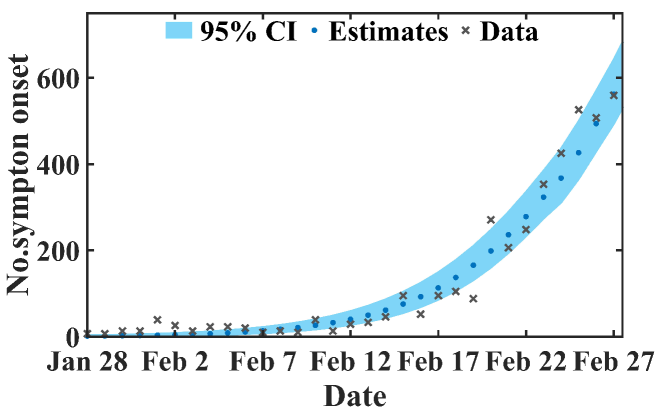
Supplementary Figure S7: Validation of our backtracking method. The validation method is based on the data of early laboratory-confirmed cases in Lombardy area (January 28 - February 27, 2020). The incidence data of patients are estimated from the laboratory reported confirmed cases and the distribution of the time delay between the onset of the disease and the reported confirmation. The blue dots and black crosses represent, respectively, the incidence estimation curve and the retrospective survey data of laboratory-confirmed cases in the literature [35]. The light blue shaded region represents the 95% confidence interval of the estimation.

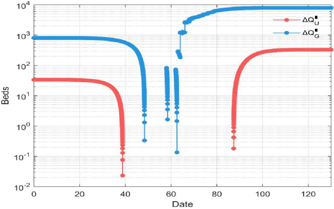
Supplementary Figure S8: Remaining resources of GW and ICU in Wuhan after two admission processes. The ordinate is on a logarithmic scale, and the red and blue dots indicate that the amounts of remaining resources of Wuhan ICU and GW at time $t$ are $\Delta Q_{U}(t)$ and $\Delta Q_{G}(t)$, respectively. The missing areas of the red and blue dots represent the period of $\Delta Q_{U}=0$ and $\Delta Q_{G}=0$, respectively.

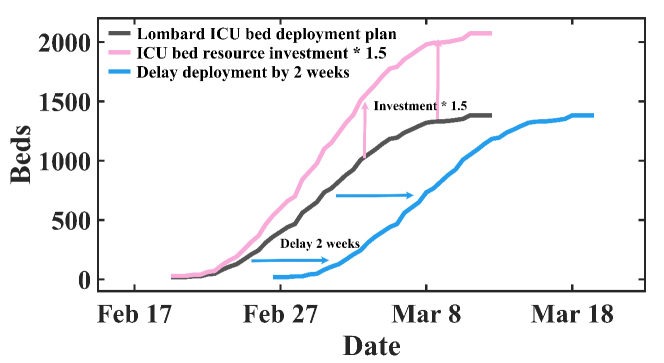
Supplementary Figure S9: Effects of varying ICU deployment plan in Lombardy, Italy. The black curve shows Lombardy’s actual ICU medical resource deployment plan, as displayed in Tab. S4. The blue and red curves show the two cases where Lombardy’s government would delay the deployment of ICU resources by two weeks ($\mbox{DT}=14$ and $\mbox{RI}=1$) and the ICU resource is expanded by a factor of 1.5 ($\mbox{DT}=0$ and $\mbox{RI}=1.5$), respectively.

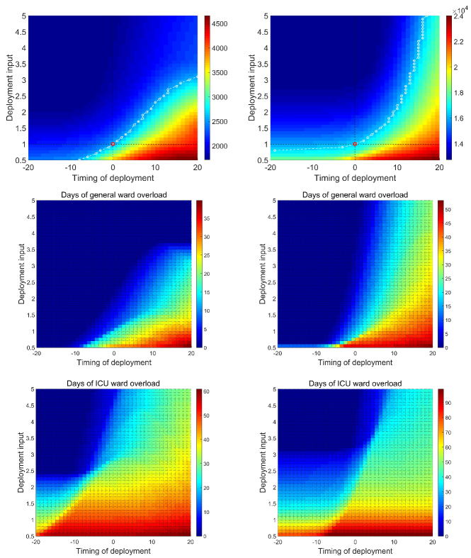
Supplementary Figure S10: Changes in the number of deaths and overload days for simultaneous GW and ICU resource deployment for Wuhan and Lombardy. (a,b) Numbers of deaths in Wuhan and Lombardy, respectively. (c,d) GW ward overload days in Wuhan and Lombardy, respectively. (e,f) ICU ward overload days in Wuhan and Lombardy, respectively.

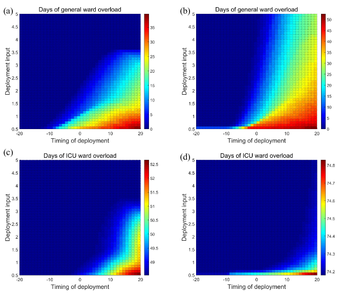
Supplementary Figure S11: Change in overload days for fixed ICU resource deployment and varying GW resource deployment. (a,b) Overload days of GW in Wuhan and Lombardy, respectively. (c,d) Overload days of ICU in Wuhan and Lombardy, respectively.

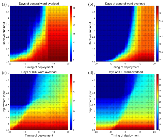
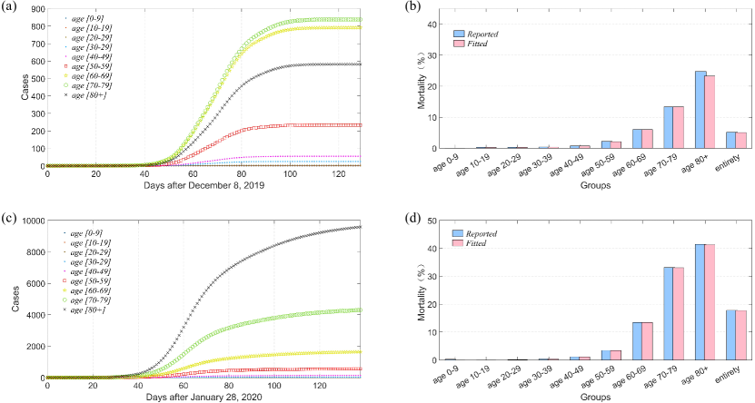
Supplementary Figure S12: Change in overload days for fixed GW resource deployment and varying ICU resource deployment. (a,b) Overload days of GW in Wuhan and Lombardy, respectively. (c,d) Overload days of ICU in Wuhan and Lombardy, respectively.

Supplementary Figure S13: Mortality rate of different age groups and evolution of the number of deaths. (a) Actual data of mortality rate of different age groups in Wuhan versus model prediction. (b) Change in the number of deaths by age groups in Wuhan. (c) Actual mortality data for all age groups in Lombardy versus model prediction. (d) Number of deaths in Lombardy in each age group. In (a) and (c), the legends from top to bottom are age [0-9] to [80]. In (b) and (d), the light blue and pink cylinders, respectively, represent the actual and simulated mortalities in each group, where the $x$-axis marks the groups with growing age.

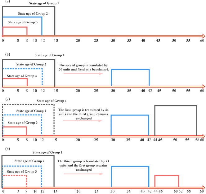
Supplementary Figure S14: Weighted state age of each age group. (a) Initial state age of the three groups of patients. (b) The state age of the second group is translated by 30 units and fixed as a benchmark. (c) The state age of the first group is translated by 44 units, and that of the third group remains unchanged. (d) The state age of the third group is translated by 44 units, and that of the first group remains unchanged.

- [1] Weekly Operational Update: Coronavirus disease 2019 (COVID-19) World Health Organization 4 September 2020 (2020).
- [2] Kraemer, M. U. et al. The effect of human mobility and control measures on the COVID-19 epidemic in China. Science 368, 493–497 (2020).
- [3] Kissler, S. M., Tedijanto, C., Goldstein, E., Grad, Y. H. & Lipsitch, M. Projecting the transmission dynamics of SARS-CoV-2 through the postpandemic period. Science 368, 860–868 (2020).
- [4] Hao, X. et al. Reconstruction of the full transmission dynamics of COVID-19 in Wuhan. Nature 584, 420–424 (2020).
- [5] Long, Y.-S. et al. Quantitative assessment of the role of undocumented infection in the 2019 novel coronavirus (COVID-19) pandemic. arXiv preprint arXiv:2003.12028 (2020).
- [6] Zhai, Z.-M. et al. State-by-State prediction of likely COVID-19 scenarios in the United States and assessment of the role of testing and control measures. medRxiv (2020). URL https://www.medrxiv.org/content/early/2020/04/29/2020.04.24.20078774.
- [7] Zhai, Z.-M., Long, Y.-S., Tang, M., Liu, Z. & Lai, Y.-C. When did COVID-19 start?-Optimal inference of time ZERO. Research Square URL https://doi.org/10.21203/rs.3.rs-48664/v1.
- [8] Flaxman, S. et al. Estimating the effects of non-pharmaceutical interventions on COVID-19 in Europe. Nature 584, 257–261 (2020).
- [9] Dehning, J. et al. Inferring change points in the spread of covid-19 reveals the effectiveness of interventions. Science 369 (2020).
- [10] Jia, J. S. et al. Population flow drives spatio-temporal distribution of COVID-19 in China. Nature 582, 389–394 (2020).
- [11] Ali, S. T. et al. Serial interval of SARS-CoV-2 was shortened over time by nonpharmaceutical interventions. Science 369, 1106–1109 (2020).
- [12] Ferguson, N. et al. Report 9: Impact of non-pharmaceutical interventions (NPIs) to reduce COVID-19 mortality and healthcare demand (2020). URL http://hdl.handle.net/10044/1/77482.
- [13] Davies, N. G. et al. Effects of non-pharmaceutical interventions on COVID-19 cases, deaths, and demand for hospital services in the UK: a modelling study. The Lancet Public Health 5, E375–E385 (2020).
- [14] Miller, I. F., Becker, A. D., Grenfell, B. T. & Metcalf, C. J. E. Disease and healthcare burden of COVID-19 in the United States. Nature Medicine 26, 1212–1217 (2020).
- [15] Emanuel, E. J. et al. Fair allocation of scarce medical resources in the time of Covid-19. The New England Journal of Medicine 382, 2049–2055 (2020).
- [16] White, D. B. & Lo, B. A framework for rationing ventilators and critical care beds during the COVID-19 pandemic. JAMA 323, 1773–1774 (2020).
- [17] Wang, D. et al. Clinical characteristics of 138 hospitalized patients with 2019 novel coronavirus–infected pneumonia in Wuhan, China. JAMA 323, 1061–1069 (2020).
- [18] Yang, X. et al. Clinical course and outcomes of critically ill patients with SARS-CoV-2 pneumonia in Wuhan, China: a single-centered, retrospective, observational study. The Lancet Respiratory Medicine 8, 475–481 (2020).
- [19] Grasselli, G. et al. Baseline characteristics and outcomes of 1591 patients infected with SARS-CoV-2 admitted to ICUs of the Lombardy Region, Italy. JAMA 323, 1574–1581 (2020).
- [20] Garg, S. Hospitalization rates and characteristics of patients hospitalized with laboratory-confirmed coronavirus disease 2019—COVID-NET, 14 States, March 1–30, 2020. MMWR Morb Mortal Wkly Rep 69, 458–464 (2020).
- [21] Novel, C. P. E. R. E. et al. The epidemiological characteristics of an outbreak of 2019 novel coronavirus diseases (COVID-19) in China. Zhonghua Liu Xing Bing Xue Za Zhi 41, 145 (2020).
- [22] COVID, T. C. & Team, R. Severe Outcomes Among Patients with Coronavirus Disease 2019 (COVID-19)-United States, February 12-March 16, 2020. MMWR Morb Mortal Wkly Rep 69, 343–346 (2020).
- [23] https://www.epicentro.iss.it/coronavirus/sars-cov-2-dashboard (2020).
- [24] http://mzj.wuhan.gov.cn/zwgk_918/fdzdgk/ggfw/shfl/201901/t20190125_1000644.shtml (2020).
- [25] https://www.citypopulation.de/en/italy/localities/lombardia/ (2020).
- [26] http://www.salute.gov.it/imgs/c_17_notizie_4640_0_file.pdf (2020).
- [27] Gaythorpe, K. et al. Report 8: Symptom progression of COVID-19 (2020).
- [28] Zhou, F. et al. Clinical course and risk factors for mortality of adult inpatients with COVID-19 in Wuhan, China: a retrospective cohort study. The Lancet 395, 1054–1062 (2020).
- [29] Pan, A. et al. Association of public health interventions with the epidemiology of the COVID-19 outbreak in Wuhan, China. JAMA 323, 1915–1923 (2020).
- [30] Cereda, D. et al. The early phase of the COVID-19 outbreak in Lombardy, Italy. arXiv preprint arXiv:2003.09320 (2020).
- [31] https://en.wikipedia.org/wiki/covid-19_pandemic_in_italy (2020).
- [32] http://wjw.wuhan.gov.cn/ (2020).
- [33] Tibshirani, R. J. & Efron, B. An introduction to the bootstrap. Mono. Stat. Appl. Prob. 57, 1–436 (1993).
- [34] Chowell, G. Fitting dynamic models to epidemic outbreaks with quantified uncertainty: A primer for parameter uncertainty, identifiability, and forecasts. Infect. Dis. Model. 2, 379–398 (2017).
- [35] https://en.calameo.com/books/005243496f711f39d24b9 (2020).
- [36] https://covid19.healthdata.org/italy/lombardia (2020).
- [37] https://www.qianzhan.com/analyst/detail/220/200312-d2e29fce.html (2020).
- [38] https://www.statista.com/chart/21105/number-of-critical-care-beds-per-100000-inhabitants/ (2020).
- [39] https://www.insidermonitor.com/covid19/zh/ (2020).