Introduction to Isolated Horizons in Numerical Relativity

Abstract

We present a coordinate-independent method for extracting mass ($M_{\Delta}$) and angular momentum ($J_{\Delta}$) of a black hole in numerical simulations. This method, based on the isolated horizon framework, is applicable both at late times when the black hole has reached equilibrium, and at early times when the black holes are widely separated. Assuming that the spatial hypersurfaces used in a given numerical simulation are such that apparent horizons exist and have been located on these hypersurfaces, we show how $J_{\Delta}$ and $M_{\Delta}$ can be determined in terms of only those quantities which are intrinsic to the apparent horizon. We also present a numerical method for finding the rotational symmetry vector field (required to calculate $J_{\Delta}$) on the horizon.

I Introduction

Given a numerical simulation of a spacetime containing a black hole, one is faced with two immediate questions: Where is the black hole, and what are the values of its parameters, such as mass and angular momentum?

In analytical considerations, a black hole is often defined via the event horizon, i.e. the future boundary of the causal past of future null infinity. While this notion is mathematically elegant and has led to powerful results in black hole physics, generally it is not directly useful in numerical evolutions of black hole spacetimes. The reason is the teleological nature of the event horizon: it can be constructed only after we have knowledge of the entire spacetime and spacetime is the end product of these simulations. Furthermore, due to practical limitations, generally one cannot evolve all the way to future null infinity. For such reasons, in numerical evolutions, it is more common to use apparent horizons to characterize a black hole. Apparent horizons are closed two-surfaces on a spatial slice of the spacetime and are, therefore, well suited to numerical simulations that evolve data from one spatial slice to another. While it is possible that there exist no apparent horizons on the spatial slices used in a given numerical simulation of a black hole spacetime, in practice, this issue does not arise for most numerical black hole simulations that we are aware of. We shall therefore disregard this issue for the rest of this paper and only deal with partial Cauchy surfaces (in black hole spacetimes) for which apparent horizons do exist and have been located t ; bcsst ; aclmss ; hcm ; a ; dhm ; es . A natural question we want to ask is: can one unambiguously associate black hole parameters to apparent horizons?

One way to attribute a mass and an angular momentum to a black hole is to calculate the corresponding ADM quantities at infinity. The main difficulty is that the ADM mass and angular momentum refer to the whole spacetime. In a dynamical situation, such a spacetime will contain gravitational radiation and it is not clear how much of the mass or angular momentum should be attributed to the black hole itself and, if there is more than one black hole, to each individual black hole.

It is desirable to have a framework that combines the properties of apparent horizons with the powerful tools available at infinity. In the regime when the black hole is isolated in an otherwise dynamical spacetime, such a framework now exists in the form of isolated horizons abf ; letter ; afk ; abl1 ; abl2 . In numerical simulations of, say, black hole collisions, the black hole would be isolated at early times when the black holes are well separated, or at late times when the final black hole has settled down, but radiation is still present in the spacetime. Isolated horizons provide a way to identify a black hole quasi-locally, and allow for the calculation of mass and angular momentum. It has been shown recently that the formulae for angular momentum and mass arising from the isolated horizon formalism are valid even in dynamical situations ak . Therefore, the numerical methods presented in this article are relevant even for fully dynamical black holes.

The aim of this paper is to introduce the isolated horizon framework in a way that is directly useful in numerical relativity. In particular, we show how to find isolated horizons numerically, and how to implement the isolated horizon formulae for $J_{\Delta}$ and $M_{\Delta}$. A key result of this paper is that, to find the angular momentum of an isolated horizon, one can just use the ADM formula for angular momentum but now applied at the apparent horizon. This is not an assumption, but a rigorous result obtained by calculating the Hamiltonian generating diffeomorphisms which reduce to rotational symmetries on the isolated horizon. This is completely analogous to what is done at infinity to obtain the ADM formulae for mass and angular momentum for asymptotically flat spacetimes. Indeed, the Hamiltonian analysis of isolated horizons is an extension of the ADM formalism to the case where the region of spacetime under consideration has an inner boundary in the form of an isolated horizon. The isolated horizon results for $J_{\Delta}$ and $M_{\Delta}$ are also convenient for practical reasons because their expressions only involve data defined on the apparent horizon. An important ingredient in the formula for $J_{\Delta}$ is an axial symmetry vector on the apparent horizon. Therefore we also present and implement a numerical method for locating Killing vectors on the horizon.

This paper is organized as follows. In section II we first review the notion of isolated horizons and explain how they can be located in numerical simulations of black hole spacetimes. We also explain their relation to apparent horizons and give the formulae for their mass and angular momentum. These formulae require that we find a Killing vector on the apparent horizon. A method for doing this is described in section III. Section IV describes the practical numerical implementation of these formulae, and we verify that our method gives the expected results in the simple case of a boosted Kerr black hole. Section V compares the isolated horizon formulae with other approaches used to compute mass and angular momentum, and finally in section VI we give some possible applications and future directions.

II Isolated Horizons

Let us first fix our notation. The spacetime metric is taken to have signature $(-,+,+,+)$, and we use geometrical units where $G$ and $c$ are equal to unity. We will usually use the abstract index notation, but occasionally, especially for differential forms, the index free notation will also be used. The Riemann tensor ${R_{abc}}^{d}$ will be defined by the equation $2\nabla\!_{[a}\nabla\!_{b]}\alpha_{c}={R_{abc}}^{d}\alpha_{d}$ where $\alpha_{a}$ is an arbitrary co-vector. We work on a spacetime that is foliated by a spatial three manifold $\Sigma$ which is a partial Cauchy surface. The spacetime is thus of the form $\Sigma\times\mathbb{R}$. The three-metric and extrinsic curvature on a spatial slice $\Sigma$ are respectively denoted by $\gamma_{ab}$ and $K_{ab}:=-{\gamma_{a}}^{c}{\gamma_{b}}^{d}\nabla\!_{c}T_{d}$ where $T^{a}$ is the unit timelike normal to $\Sigma$. The two-metric on the apparent horizon is called $q_{ab}$. All manifolds and fields will be taken to be smooth. Finally, though it is quite easy to include matter fields, we will be interested in vacuum spacetimes only. This paper is reasonably self contained, however, for precise and detailed definitions and proofs we refer the reader to abf ; afk ; abl1 ; abl2 . In this paper we shall focus on the basic physical ideas underlying the isolated horizon framework and its application to numerical relativity.

II.1 Motivation, definition and basic results

For completeness and to fix notation, let us start by reviewing the definition of apparent horizons. Let $T^{a}$ be the unit timelike vector field orthogonal to a partial Cauchy surface $\Sigma$. Given a closed two-surface $S\subset\Sigma$, we have the unique unit outward-pointing spacelike normal $R_{a}$ which is tangent to $\Sigma$. We are assuming here that one can define what is meant by the inside and outside of $S$. This can be done, for instance, by imposing certain global conditions on the spacetime and the partial Cauchy surfaces under consideration. These conditions include: asymptotic flatness, strong future asymptotic predictability of the spacetime with the Cauchy surfaces under consideration and certain topological restrictions on $\Sigma$. Since the focus of this paper is not on such global topological properties of spacetimes, we shall not spell out these assumptions precisely and instead refer the reader to hawk . It is worth mentioning that the inside and outside $S$ can also be defined quasi-locally without using global assumptions such as the ones mentioned above. This has been done by Hayward sh using the notion of trapping horizons which we discuss in a later section.

Let $q_{ab}$ be the induced Riemannian two-metric on $S$ and $\epsilon_{ab}$ the area two-form on $S$ constructed from $q_{ab}$. We can construct a convenient basis for performing calculations at points of $S$ in a natural way (see figure 1). First, define the outgoing and ingoing null vectors

$$\ell^{a}:=\frac{1}{\sqrt{2}}(T^{a}+R^{a})\quad\textrm{and}\quad n^{a}:=\frac{1}{\sqrt{2}}(T^{a}-R^{a})\,.$$ (1)

It is worth noting that any spacelike two-surface $S$ determines uniquely, up to rescalings, two null vectors orthogonal to $S$. Any other choice of $\ell$ and $n$ will differ from the one made in equation (1) only by possible rescalings. We tie together the scalings of $\ell$ and $n$ by requiring $\ell\cdot n=-1$.

Next, given two arbitrarily chosen spacelike orthonormal vectors $e_{1}$ and $e_{2}$ tangent to $S$, construct a complex null vector

$$m:=\frac{1}{\sqrt{2}}(e_{1}+ie_{2}).$$ (2)

It satisfies the relations $m\cdot m=0$, $m\cdot\overline{m}=1$, $\ell\cdot m=0$, and $n\cdot m=0$. Since $\ell$ and $n$ satisfy $\ell\cdot n=-1$, we see that $(\ell,n,m,\overline{m})$ form a null tetrad at $S$. This is, of course, only one possible choice of null tetrad, and we must ensure that physical results are independent of this choice.

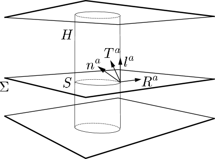
Figure 1: The figure shows an apparent horizon $S$ embedded in a spatial slice $\Sigma$. $T^{a}$ is the unit timelike normal to $\Sigma$ and $R^{a}$ is the outward pointing unit spatial normal to $S$ in $\Sigma$; $\ell^{a}$ and $n^{a}$ are the outgoing and ingoing null vectors, respectively. The vector $m^{a}$ (not shown in the figure) is tangent to $S$. $H$ is the world tube of apparent horizons.

The expansions of $\ell^{a}$ and $n^{a}$ are defined as $\theta_{(\ell)}:=q^{ab}\nabla\!_{a}\ell_{b}$ and $\theta_{(n)}:=q^{ab}\nabla\!_{a}n_{b}$, respectively. Note that in order to find the expansions, we only need derivatives of $\ell$ and $n$ along $S$, and there is no need to extend the null tetrad into the full spacetime. However, if in some numerical computations it is necessary to extend the null tetrad smoothly into the full spacetime; all calculations will be insensitive to this extension. The surface $S$ is said to be an apparent horizon if it is the outermost outer-marginally-trapped-surface, i.e. it is the outermost surface on $\Sigma$ with $\theta_{(\ell)}=0$ and $\theta_{(n)}<0$.

Consider now the world tube of apparent horizons $H$ constructed by stacking together the apparent horizons on different spatial slices. As we shall show later in section II.2, smooth segments of this world tube are generically spacelike; it is null when no matter or radiation is falling into the black hole. At late times, one expects the black hole to reach equilibrium when radiation and matter are no longer crossing the horizon. In this regime, the world tube $H$ will be a null surface, and the two-metric $q_{ab}$ on the apparent horizon $S$ may now be viewed as a degenerate three-metric on the null surface $H$. Furthermore, from experience with numerical simulations and also from general topological censorship results (see e.g. fsw ), we know that at late times, the apparent horizons must have spherical topology. Therefore, at late times, the topology of $H$ is $S^{2}\times\mathbb{R}$. Finally, in this regime, the outward-normal $\ell$ constructed in equation (1) is a null normal to the world tube $H$, and most importantly, from the definition of an apparent horizon, the outward normal $\ell$ is always expansion free.

We will now argue that the isolated horizon framework is ideally suited to describe apparent horizons in the regime when the world tube $H$ is null. For our purposes, the straightforward definition of a non-expanding horizon given below shall suffice. To carry out the Hamiltonian analysis in order to define mass and angular momentum, we actually need to impose further conditions on non-expanding horizons, which we shall briefly describe towards the end of this section. The formulae for mass and angular momentum make sense even on non-expanding horizons.

Definition: A three dimensional sub-manifold $\Delta$ of a space-time $(\mathcal{M},g_{ab})$ is said to be a non-expanding horizon (NEH) if it satisfies the following conditions:

(i) $\Delta$ is topologically $S^{2}\times\mathbb{R}$ and null;

(ii) The expansion $\theta_{(\ell)}:=q^{ab}\nabla_{a}\ell_{b}$ of $\ell$ vanishes on $\Delta$, where $\ell$ is any null normal to $\Delta$;

(iii) All equations of motion hold at $\Delta$ and, if any matter field are present with $T_{ab}$ as the stress energy tensor, then we require $-T_{b}^{a}\ell^{b}$ to be future directed and causal for any future directed null normal $\ell^{b}$.

Note that if condition (ii) holds for one null normal $\ell$, then it holds for all. We will only consider those null normals which are nowhere vanishing and future directed. We are therefore allowed to rescale $\ell$ by any positive-definite function. The energy condition in (iii) is implied e.g. by the null energy condition which is commonly assumed; for the remainder of this paper, we shall usually consider only vacuum spacetimes.

Comparing the properties of the world tube $H$ described earlier with conditions (i) and (ii) in the definition, we see that the NEH is precisely what we need to model the physical situation at hand; when the black hole is approximately isolated, the world tube $H$ represents a non-expanding-horizon $\Delta$. The motivation behind the conditions in the definition are thus rather straightforward from the perspective of apparent horizons.

We have motivated the above definition using the world tube of apparent horizons which in general clearly depends on how we choose to foliate the spacetime with spatial surfaces. It is then natural to ask whether an NEH depends on the choice of this foliation. To avoid unnecessary technicalities, let us consider a possibly dynamical spacetime containing one isolated black hole. As mentioned in the introduction, we can choose spatial hypersurfaces on which there are no apparent horizons so that the world tube of apparent horizons does not exist for this foliation. Let us ignore this possibility and focus on the case when each spatial slice has exactly one marginally trapped surface and hence exactly one apparent horizon; the generalization to multi black hole spacetimes is straightforward. It is not difficult to verify that the world tube of apparent horizons is independent of the spacelike hypersurfaces used to construct it. In other words, the null surface (the NEH) obtained by stacking together all the apparent horizons at different times is independent of how we choose to foliate the spacetime by spacelike hypersurfaces; this is not true in the regime when the horizon is non-isolated and the world tube is spacelike. An NEH, even when viewed as the world tube of apparent horizons, is therefore an invariant notion in the four dimensional spacetime. Every cross section of an NEH is potentially an apparent horizon if it arises as the intersection of the NEH with a spatial slice. Choosing a different spatial slice corresponds to obtaining a different cross section of the NEH. As we shall see later, for calculating physical quantities such as angular momentum and mass, it does not matter which cross section of the NEH we choose to work with.

Even though cross sections of an NEH are very closely related to apparent horizons, there are two differences: (i) Apparent horizons are required to be the outermost surfaces on a spatial slice with the afore-mentioned properties. This may not be true in general for cross sections of $\Delta$; (ii) Since they are trapped surfaces, apparent horizons also satisfy the condition $\theta_{(n)}<0$. Though this will most likely be true in actual numerical simulations, it turns out that this condition is not required to study the mechanics of isolated horizons. In fact, there exist exact solutions representing black holes which are isolated horizons but do not satisfy $\theta_{(n)}<0$, e.g., the distorted black holes studied by Geroch and Hartle gh . In these solutions the integral of $\theta_{(n)}$ over a cross section of the horizon is still negative even though $\theta_{(n)}$ is not necessarily negative everywhere. In the remainder of this paper, we shall ignore these caveats and the phrases ‘apparent horizon’ and ‘cross-section of $\Delta$’ will be used interchangeably.

Consequences of the definition: The simple definition of a NEH leads to a surprisingly large number of consequences. The important results we shall need later are the existence of a one-form $\omega_{a}$ whose definition is given in equation (3), and the fact that the component $\Psi_{2}$ of the Weyl tensor is a physical, i.e. gauge invariant, property of an isolated horizon. Keeping these two results in mind, the rest of this sub-section may be skipped on a first reading.

While stating the results, it is convenient to use a null-tetrad $(\ell,n,m,\overline{m})$ which is adapted to the horizon; this means that $\ell$ is a (future directed) null normal to $\Delta$. An example of such a null-tetrad is the one constructed in equations (1) and (2), but there is, of course, an infinity of such tetrads. Physical quantities will be independent of which null-tetrad we choose. These consequences do not require the spacetime to be vacuum; they only assume the energy condition mentioned after the definition above.

• Area of apparent horizons is constant: Any null normal $\ell$ is always geodetic and is also a symmetry of the degenerate intrinsic metric $q_{ab}$ on $\Delta$: ${\cal L}\,_{\ell}q_{ab}\triangleq 0$ (the symbol ‘$\triangleq$’ means that the equality holds only at points of $\Delta$). Furthermore, the area of any cross-section $S$ defined as $A_{\Delta}:=\oint_{S}\textrm{d}^{2}V$ is the same where $\textrm{d}^{2}V$ is the natural area measure on $S$ constructed from the two-metric $q_{ab}$. In particular, the area of the apparent horizons is constant in time.

• Definition of $\omega_{a}$: It will be shown in section II.2 that the shear of $\ell$ defined as $\sigma_{(\ell)}:=m^{a}m^{b}\nabla\!_{a}\ell_{b}$ is zero. The twist of $\ell$ is trivially zero because $\ell$ is normal to a smooth surface, and the expansion of $\ell$ is zero by definition. Since the null normal $\ell$ is expansion, twist and shear free, there must exist a one-form $\omega_{a}$ intrinsic to $\Delta$ such that

  $$t^{a}\nabla\!_{{a}}\ell^{b}\triangleq t^{a}\omega_{a}\ell^{b}$$ (3)

  for any vector $t^{a}$ tangent to $\Delta$. If the null normal $\ell$ is rescaled $\ell\rightarrow\tilde{\ell}=f\ell$, the one-form $\omega_{a}$ transforms as

  $$\omega\rightarrow\tilde{\omega}=\omega+\textrm{d}\left(\ln f\right)$$ (4)

  where ‘d’ is the exterior derivative on $\Delta$.

• Gauge invariance of $\Psi_{2}$: If we choose a null tetrad adapted to $\Delta$ such as in equations (1) and (2), then we get the following restrictions on the Weyl tensor $C_{abcd}$ at $\Delta$ afk :

  $$\Psi_{0}\triangleq\Psi_{1}\triangleq 0$$ (5)

  and

  $$\textrm{d}\omega\triangleq 2{\mathrm{Im}}\left[\Psi_{2}\right]\,\epsilon,$$ (6)

  where

  $$\Psi_{0} = C_{abcd}\ell^{a}m^{b}\ell^{c}m^{d}$$ (7)

  $$\Psi_{1} = C_{abcd}\ell^{a}m^{b}\ell^{c}n^{d}$$ (8)

  $$\Psi_{2} = C_{abcd}\ell^{a}m^{b}\overline{m}^{c}n^{d}$$ (9)

  and $\epsilon$ is the area two-form on the apparent horizon. This can be used to prove the important result that $\Psi_{2}$ is gauge invariant. The gauge freedom we are concerned with here is the choice of null tetrads adapted to $\Delta$. The allowed gauge transformations relating different choices are null rotations about $\ell$:

  $$\ell \rightarrow \ell$$

  $$m \rightarrow m+\overline{c}\ell$$ (10)

  $$n \rightarrow n+cm+\overline{c}\overline{m}+c\overline{c}\ell$$

  and spin-boost transformations:

  $$\ell \rightarrow A\ell$$

  $$n \rightarrow A^{-1}n$$ (11)

  $$m \rightarrow e^{2i\theta}m$$

  Here $c$, $A$ and $\theta$ are arbitrary smooth functions on $\Delta$. It turns out that $\Psi_{2}$ is always invariant under spin-boost transformations; under null rotations, it transforms as (see e.g. the appendix of s )

  $$\Psi_{2}\rightarrow\Psi_{2}+2c\Psi_{1}+c^{2}\Psi_{0}\,.$$ (12)

  Since $\Psi_{0}$ and $\Psi_{1}$ vanish at $\Delta$, we see that $\Psi_{2}$ is in fact gauge invariant at the horizon: it does not depend on the choice of null tetrad as long as $\ell$ is one of the null generators of $\Delta$. This property is important because it tells us that the value of $\Psi_{2}$ at the horizon does not depend on how we choose to foliate our spacetime. A different spatial slice $\tilde{\Sigma}$ will lead to a different $\tilde{\ell}$, $\tilde{n}$ and $\tilde{m}$. The two null tetrads will be related by a combination of the following transformations: a null-rotation about $\ell$, a spin-boost transformation, or a multiplication of $m$ by a phase. Whichever null-tetrad we use to calculate $\Psi_{2}$, we will get the same result. As we shall see, it is the imaginary part of $\Psi_{2}$ which is physically interesting for our purposes.

Further Definitions: The notion of non-expanding horizons describes the late time behavior of apparent horizons. In order to define the mass $M_{\Delta}$ and angular momentum $J_{\Delta}$ of $\Delta$, one needs to go beyond this definition and introduce additional structures on the horizon. This is done via the definition of a weakly isolated horizon afk ; abl1 . The Hamiltonian analysis which leads to the definitions of mass and angular momentum requires this extra structure. Fortunately, it turns out that the formulae for $M_{\Delta}$ and $J_{\Delta}$ do not depend on this extra structure and hold true for non-expanding horizons. We could therefore omit these definitions entirely and simply state the results of the calculation. For the sake of completeness, we shall give the basic idea behind weakly isolated horizons. The rest of this sub-section may be skipped without loss of continuity.

In an NEH, the intrinsic metric $q_{ab}$ is time independent since ${\cal L}\,_{\ell}q_{ab}\triangleq 0$. There is no restriction on the time derivatives of the extrinsic curvature of $\Delta$ or the intrinsic connection on $\Delta$ (by ‘time derivative’ we mean derivative along $\ell$). Since $\Delta$ is a null surface, there is no natural notion of extrinsic curvature. The closest thing to extrinsic curvature is the tensor ${K_{a}}^{b}$ defined via $t^{a}{K_{a}}^{b}\triangleq t^{a}\nabla\!_{a}\ell^{b}$ for any $t^{a}$ tangent to $\Delta$. This tensor is known in the mathematics literature as the Weingarten map, and as its definition shows, it is $\nabla\!_{a}\ell^{b}$ with the covariant index pulled back to $\Delta$. From equation (3) we immediately obtain ${K_{a}}^{b}\triangleq\omega_{a}\ell^{b}$. This implies that requiring ${K_{a}}^{b}$ to be time independent is equivalent to requiring ${\cal L}\,_{\ell}\omega_{a}\triangleq 0$. Unfortunately, due of the transformation property of $\omega_{a}$ (see equation (4)), it is clear that this equation is not meaningful if all rescalings of $\ell$ are allowed. Note that if we restrict ourselves to rescalings that are constant on the horizon, then $\omega_{a}$ is invariant. We thus need to restrict ourselves to an equivalence class of null normals $[\ell]$, the members of which are related to each other by a constant, positive non-zero rescaling. We can then associate a unique $\omega_{a}$ with $[\ell]$. The equation ${\cal L}\,_{\ell}\omega_{a}\triangleq 0$ is now perfectly meaningful if $\ell$ is a member of $[\ell]$. A weakly isolated horizon is then defined as an NEH $\Delta$ equipped with such a preferred equivalence class of null normals $[\ell]$. Furthermore, the $\omega_{a}$ associated with $[\ell]$ must be time independent: ${\cal L}\,_{\ell}\omega_{a}\triangleq 0$. Given an NEH, we can always find such a preferred equivalence class (but this equivalence class is not unique). Thus every NEH can be turned into a weakly isolated horizon. The Hamiltonian analysis of weakly isolated horizons leads to formulae for mass and angular momentum, and as we shall see in section II.3, these formulae are insensitive to arbitrary rescalings of $\ell$ and thus they make sense even for non-expanding horizons.

We can introduce an even stronger definition. A weakly isolated horizon requires that $\omega_{a}$ be time independent. It can be seen from equation (3) that $\omega_{a}$ is also a component of the intrinsic connection $D_{a}$ induced on $\Delta$ by the four dimensional connection $\nabla\!_{a}$ compatible with the four-metric. However, $\omega_{a}$ is just one component of $D_{a}$. In an isolated horizon, we require that all components of $D_{a}$ are time independent. It turns out that generically, this condition gives us a preferred unique equivalence class $[\ell]$ abl2 .

II.2 Finding non-expanding horizons

Our strategy to find non-expanding horizons is to locate apparent horizons on each spatial slice and then to check whether the world tube $H$ obtained by stacking these horizons together is a NEH. What remains to be checked is whether the tube is a null surface. By definition, a surface is null if the metric $h_{ab}$ induced on this surface has a degenerate direction, i.e. if there exists a vector $X^{a}$ tangent to $H$ such that $h_{ab}X^{b}=0$; therefore, one possible method to check whether $H$ is isolated is to construct the induced metric $h_{ab}$ on $H$ and see if it has a zero eigenvalue. To construct $h_{ab}$ numerically, we have to know the two-metric $q_{ab}$ on at least two different time slices. Furthermore, in a numerical simulation, $H$ will never be exactly isolated because of numerical errors, and it is not clear how this method can quantify how close the horizon is to being exactly isolated. Fortunately, there is a much simpler method which only requires the two-metric on a single time slice and can also provide a quantitative measure of how close $H$ is to being perfectly isolated. This method is based on the shear $\sigma^{(\ell)}_{ab}$ of $\ell$, which is the symmetric trace-free part of the projection of $\nabla\!_{a}\ell_{b}$ onto the apparent horizon $S$. The tensor $\sigma^{(\ell)}_{ab}$ has two independent components, and is conveniently written in terms of a single complex number $\sigma_{(\ell)}:=m^{a}m^{b}\nabla\!_{a}\ell_{b}$, where $m$ is defined in equation (2). To calculate $\sigma_{(\ell)}$ conveniently, we simply decompose $\ell$ using equation (1):

$$\sigma_{(\ell)} \triangleq m^{a}m^{b}\nabla\!_{a}\ell_{b}$$ (13)

$$\triangleq \frac{1}{\sqrt{2}}m^{a}m^{b}\nabla\!_{a}T_{b}+\frac{1}{\sqrt{2}}m^{a}m^{b}\nabla\!_{a}R_{b}\,.$$

In the above equation, we have extended the notation ‘$\triangleq$’ to also mean that the equality holds only at points of $H$. The first term is just a component of the extrinsic curvature $K_{ab}$, while the second term can be calculated on the spatial slice by calculating the connection associated with the three-metric $\gamma_{ab}$. We shall now prove the following important result concerning $\sigma_{(\ell)}$:

The world tube of apparent horizons is a NEH if and only if $\sigma_{(\ell)}\triangleq 0$.

Readers not interested in the proof of this statement can skip forward to equation (20).

To prove this statement, we need to consider the general case when $H$ is not null. This has been studied in great detail by Hayward sh . In Hayward’s terminology, the surface $H$ is essentially a future outer trapping horizon. This means that $H$ is foliated by a family of marginally trapped surfaces (which in our case are the apparent horizons) satisfying the relations $\theta_{{(\ell)}}\triangleq 0$, $\theta_{{(n)}}<0$ and ${\cal L}\,_{n}\theta_{{(\ell)}}<0$. These are physically very reasonable conditions, and all black holes found in simulations are expected to satisfy them. Incidentally, note that the condition ${\cal L}\,_{n}\theta_{{(\ell)}}\triangleq 0$ can be used to define, in a quasi local manner, what we mean by the inside and outside of the horizon.

The proof of this statement, adapted from sh , is then quite simple: let $z^{a}$ be a vector tangent to $H$ and orthogonal to the foliation whose leaves are the apparent horizons. Such a vector field may be considered to define time evolution at the horizon. It is easy to see that, up to a rescaling, $z^{a}$ can be expressed as a linear combination of $\ell^{a}$ and $n^{a}$

$$z^{a}\triangleq\ell^{a}-\alpha n^{a}$$ (14)

where $\alpha$ is a smooth function on $H$. The rescaling freedom in $z$ will be inconsequential for our purposes. The surface $H$ is null, spacelike, or timelike if and only if $\alpha$ is zero, positive, or negative respectively. We will now show that $\alpha\geq 0$. From the definition of apparent horizons we know that the expansion $\theta_{{(\ell)}}$ vanishes everywhere on the horizon, therefore ${\cal L}\,_{z}\theta_{{(\ell)}}\triangleq 0$. This in turn gives

$$\alpha\triangleq\frac{{\cal L}\,_{\ell}\theta_{{(\ell)}}}{{\cal L}\,_{n}\theta_{{(\ell)}}}\,.$$ (15)

Even though $\theta_{(\ell)}$ and $\theta_{(n)}$ are so far defined only on $H$, in equation (15) (and also in the very definition of a trapping horizon) we are taking the derivatives of these quantities along $\ell$ and $n$ which are not necessarily tangent to $H$. To make sense of this equation we need to extend $\ell$ and $n$ in a neighborhood of the surface $S$. This can easily be done by using the unique geodesics determined by these vectors.

The Raychaudhuri equation for $\ell$ then leads to

$${\cal L}\,_{\ell}\theta_{{(\ell)}}\triangleq-|\sigma_{{(\ell)}}|^{2}-\Phi_{00}$$ (16)

where $\Phi_{00}=\frac{1}{2}R_{ab}\ell^{a}\ell^{b}$. If we assume that the spacetime is vacuum, then $\Phi_{00}=0$, and therefore ${\cal L}\,_{\ell}\theta_{{(\ell)}}\triangleq-|\sigma_{{(\ell)}}|^{2}$, which along with equation (15) gives

$$\alpha\triangleq-\frac{|\sigma_{(\ell)}|^{2}}{{\cal L}\,_{n}\theta_{(\ell)}}\,.$$ (17)

This immediately implies that $\alpha\triangleq 0$ (which is equivalent to $H$ being null) if and only if $\sigma_{{(\ell)}}\triangleq 0$. This is what we wanted to show. More generally, since ${\cal L}\,_{n}\theta_{(\ell)}<0$, this shows that $\alpha\geq 0$, which means that $\Delta$ is spacelike when the shear is non-zero.

As a side remark we also show that $H$ is null if and only if the area element on the apparent horizons $\epsilon_{ab}$ is preserved in time. To show this we need the equations

$${\cal L}\,_{\ell}\epsilon_{ab}\triangleq\theta_{{(\ell)}}\epsilon_{ab}\triangleq 0\qquad\textrm{and}\qquad{\cal L}\,_{n}\epsilon_{ab}\triangleq\theta_{{(n)}}\epsilon_{ab}\,.$$ (18)

It then follows that

$${\cal L}\,_{z}\epsilon_{ab}\triangleq{\cal L}\,_{\ell}\epsilon_{ab}-{\cal L}\,_{\alpha n}\epsilon_{ab}\triangleq-\alpha\theta_{{(n)}}\epsilon_{ab}$$ (19)

therefore $\alpha\triangleq 0$ if and only if ${\cal L}\,_{z}\epsilon_{ab}\triangleq 0$, which is what we wanted to prove. This implies that if $\alpha\triangleq 0$, then the area of cross-sections of $\Delta$ is constant. However, the converse is not necessarily true, because $\epsilon_{ab}$ could be changing in such a way that its integral is constant; the area can be constant globally without being constant locally. Thus, in principle, we can have situations in which the area is constant without the horizon being isolated. However, constancy of area is still a very useful first check to see when the horizon reaches equilibrium. Finally, as a side remark we note that since $\alpha\geq 0$ and $\theta_{{(n)}}<0$, we get ${\cal L}\,_{z}A_{\Delta}\geq 0$, which is the area increase law.

In this paper we are interested in the case when $\sigma_{(\ell)}$ vanishes (up to numerical errors). In order for the horizon to be isolated we should have

$$s:=\oint_{S}|\sigma_{(\ell)}|^{2}\,\textrm{d}^{2}V=0$$ (20)

where $\textrm{d}^{2}V$ is the natural area measure on $S$ constructed from $q_{ab}$. The quantity $s$ is dimensionless since $\sigma_{(\ell)}$ has dimensions of inverse length. For the horizon to be numerically isolated, we require that $s$ converge to zero appropriately when the numerical resolution is increased .

II.3 Mass and angular momentum

Now let us define angular momentum. The details and proofs of the results below can be found in abl1 . In order to define the angular momentum, we need to assume that $S$ is axisymmetric, i.e. there is a vector field $\varphi^{a}$ tangent to $S$ such that it preserves $q_{ab}$ 

$${\cal L}\,_{\varphi}q_{ab}\triangleq 0\,.$$ (21)

The next section describes a simple method for finding $\varphi^{a}$. Note that $\varphi^{a}$ is not a Killing vector of the full spacetime metric. It is completely intrinsic to $\Delta$, and in fact we only need data on the apparent horizon to find it.

Given $\varphi^{a}$ and $\omega_{a}$ (defined in equation (3)), the isolated horizon angular momentum $J_{\Delta}$ is defined as the surface term at $\Delta$ in the Hamiltonian which generates diffeomorphisms along a rotational vector field which is equal to $\varphi^{a}$ at the horizon abl2 . The expression for $J_{\Delta}$ is:

$$J_{\Delta} = -\frac{1}{8\pi}\oint_{S}(\omega_{a}\varphi^{a})\,\textrm{d}^{2}V$$ (22)

$$= -\frac{1}{4\pi}\oint_{S}f{\mathrm{Im}}\left[\Psi_{2}\right]\,\textrm{d}^{2}V,$$

where $S$ is the apparent horizon and the function $f$ is related to $\varphi^{a}$ by $\partial_{a}f=\epsilon_{ba}\varphi^{b}$. In the second equality, we have used equation (5) and an integration by parts. Since $\Psi_{2}$ is gauge invariant, so is the angular momentum, and in particular, it does not depend on the scaling of $\ell$ and it thus makes sense even on a NEH. If, in a neighborhood of $\Delta$, there were a spacetime rotational Killing vector $\phi^{a}$ that approached $\varphi^{a}$ at $\Delta$, then the above formula for $J_{\Delta}$ would be equal to the Komar integral calculated for $\phi^{a}$ abl1 . However, the formula in equation (22) is more general. As a practical matter, even if there were a Killing vector in the neighborhood of $\Delta$, it is easier to use (22) rather than the Komar integral, since the Komar integral requires finding the Killing vector in the full four-dimensional spacetime. It is also worth mentioning that, if the vector field $\varphi^{a}$ is not a symmetry of $\Delta$ but is an arbitrary vector field tangent to $S$, then $J_{\Delta}$ is still the surface term at $\Delta$ in the Hamiltonian generating diffeomorphisms along vector fields which are equal to $\varphi^{a}$ at the horizon. But in this case, there would be no reason to identify $J_{\Delta}$ with the angular momentum, since conserved quantities such as mass and angular momentum are always associated with symmetries. However, the existence of the axial symmetry is the least that must be true if the horizon is to be close to Kerr in any sense. Note that angular momentum is a coordinate independent quantity; even if we use corotating coordinates to describe the black hole, the black hole still has the same angular momentum.

We now describe a form of equation (22) which is much better suited for calculating $J_{\Delta}$ numerically. From equation (3), which is the defining equation for $\omega_{a}$, we get

$$t^{a}\omega_{a}\triangleq-n_{b}t^{a}\nabla\!_{{a}}\ell^{b}\triangleq\ell^{b}t^{a}\nabla\!_{{a}}n_{b}$$ (23)

where, as before, $t^{a}$ is any vector tangent to $\Delta$. Assume that we have found the symmetry vector field $\varphi^{a}$ on the horizon (the method we use for finding $\varphi^{a}$ is described below). From equation (22), we are eventually interested in calculating $\varphi^{a}\omega_{a}$; since $\varphi^{a}$ is tangent to $\Delta$, setting $t^{a}=\varphi^{a}$ we get

$$\varphi^{a}\omega_{a} \triangleq \varphi^{a}\ell^{b}\nabla\!_{a}n_{b}$$

$$\triangleq \frac{1}{2}\varphi^{a}(T^{b}+R^{b})\nabla\!_{a}(T_{b}-R_{b})$$

$$\triangleq \frac{1}{2}\varphi^{a}(T^{b}\nabla\!_{a}T_{b}-T^{b}\nabla\!_{a}R_{b}$$

$$+R^{b}\nabla\!_{a}T_{b}-R^{b}\nabla\!_{a}R_{b})$$

$$\triangleq \varphi^{a}R^{b}\nabla\!_{a}T_{b}\triangleq-\varphi^{a}R^{b}K_{ab}$$

where we have used equation (1) along with the fact that $N^{a}$ and $R^{a}$ are orthonormal. In the last step, the definition of extrinsic curvature $K_{ab}=-\gamma_{a}^{\ c}\gamma_{b}^{\ d}\nabla\!_{c}T_{d}$ has been used where $\gamma_{ab}=g_{ab}+T_{a}T_{b}$ is the three-metric on the spatial slice $\Sigma$. We have thus reduced the calculation of $\varphi^{a}\omega_{a}$ to finding a single component of the extrinsic curvature. The integration of this scalar over the apparent horizon yields the angular momentum:

$$J_{\Delta}=\frac{1}{8\pi}\oint_{S}(\varphi^{a}R^{b}K_{ab})\,\textrm{d}^{2}V\,.$$ (25)

This is our final formula for the angular momentum. This formula is remarkably similar to the formula for the ADM angular momentum computed at spatial infinity:

$$J^{\phi}_{ADM} = \frac{1}{8\pi}\oint_{S_{\infty}}(K_{ab}-\gamma_{ab}K)\phi^{a}\,\textrm{d}^{2}S^{b}$$ (26)

$$= \frac{1}{8\pi}\oint_{S_{\infty}}K_{ab}\,\phi^{a}\,\textrm{d}^{2}S^{b}\,.$$

The $\gamma_{ab}K$ term does not contribute, because $\phi^{a}$ is tangent to $S_{\infty}$, which is the sphere at spatial infinity. Since the metric on $S_{\infty}$ is just the standard two-sphere metric, we have no difficulty in choosing a $\phi^{a}$, and we can calculate $J_{ADM}$ about any axis. In contrast, since the metric on the apparent horizon $S$ is distorted, finding $\phi^{a}$ is more complicated. Finally, as mentioned earlier, the similarity between equations (25) and (26) is not surprising, because both quantities are defined to be surface terms in Hamiltonians generating diffeomorphisms along the appropriate rotational symmetry vector fields; $J_{\Delta}$ is the surface term at $\Delta$ while $J_{ADM}^{\phi}$ is the surface term at infinity.

Given $J_{\Delta}$, the horizon mass $M_{\Delta}$ is given by afk ; abl1

$$M_{\Delta}=\frac{1}{2R_{\Delta}}\sqrt{R_{\Delta}^{4}+4J_{\Delta}^{2}}$$ (27)

where $R_{\Delta}$ is the area radius of the horizon: $R_{\Delta}=(A_{\Delta}/4\pi)^{1/2}$. This formula depends on $R_{\Delta}$ and $J_{\Delta}$ in the same way as in the Kerr solution. However, this is a result of the calculation and not an assumption. The formulae for $J_{\Delta}$ and $M_{\Delta}$ are on the same footing as the formulae for the ADM mass and angular momentum, because both are derived by Hamiltonian methods. Furthermore, under some physically reasonable assumptions on fields near future time-like infinity ($i^{+}$), one can show that $M_{\Delta}-M_{ADM}$ is equal to the energy radiated across future null-infinity if the isolated horizon extends all the way to $i^{+}$. Thus, $M_{\Delta}$ is the mass left over after all the gravitational radiation has left the system. This lends further support for identifying $M_{\Delta}$ with the mass of the black hole. Further remarks regarding equation (27) appear towards the beginning of sec. V.

To summarize: in order to calculate the mass and angular momentum of an isolated horizon, we need the following ingredients:

1. We must find the apparent horizon and check if the shear of the outward null normal vanishes within numerical errors. If it does, then the isolated horizon formulae are applicable.

2. We need to find the quantity $K_{ab}R^{b}$ on $S$ and the symmetry vector $\varphi^{a}$ (assuming it exists).

3. The angular momentum is then a simple integral over the apparent horizon given by equation (25), and the mass is a purely algebraic function given by equation (27).

The first and last steps are rather straightforward if we know the location of the apparent horizon. The only non-trivial step is the calculation of $\varphi^{a}$. In the next section, we show how it is numerically calculated using the two-metric on $S$.

III Finding the Killing Vector

First of all, we should point out that in some numerical simulations (especially simulations with built-in axi-symmetry) the axial symmetry vector is already known. In that case, one can go ahead and find the angular momentum using equation (25). However, we are also interested in the more general case, when there is an axial symmetry, but the coordinates used in the simulation are not adapted to it. In this section, we describe a general numerical method for finding $\varphi^{a}$. Our method of finding Killing vectors on the apparent horizons is based on the Killing transport equation, which we now describe. This method does not depend on the fact that we are on an apparent horizon, and it is possible that this procedure could find Killing vectors efficiently in more general situations. We first describe the general method.

Let $\xi^{a}$ be a Killing vector on $(S,q_{ab})$, and define the two-form $L_{ab}=\nabla\!_{a}\xi_{b}$. This is a two-form because of the Killing equation $\nabla\!_{(a}\xi_{b)}=L_{(ab)}=0$. It is then not difficult to prove the following (see e.g. w )

$$v^{a}\nabla\!_{a}\xi_{b} = v^{a}L_{ab}$$

$$\textrm{and}\qquad v^{a}\nabla\!_{a}L_{bc} = {R_{cba}}^{d}\xi_{d}v^{a}\,.$$ (28)

The reason for inserting an arbitrary vector $v^{a}$ will soon become clear. Instead of viewing these as equations for a Killing vector, let us instead think of them as equations for an arbitrary vector $\xi^{a}$ (or a one-form $\xi_{a}$) and an arbitrary two-form $L_{ab}$. If we start with a one-form $\xi_{a}^{(p)}$ and a two-form $L^{(p)}_{ab}$ at a point $p$ on the manifold, then the above equations can be solved along any curve $\gamma(t)$ (with $v^{a}$ as its tangent) starting at $p$ to give a unique one-form $\eta_{a}$ and a unique two-form $\alpha_{ab}$ at any other point on the curve. This procedure is analogous to parallel transport, but the differential equation used in the transport is not the geodesic equation, but instead equation (28) above, and instead of transporting a vector, these equations transport a one-form and a two-form. Viewed this way, equations (28) are often referred to as the Killing transport equations am . We are thus led to consider the vector space $V_{p}$ consisting of all pairs $(\xi^{(p)}_{a},L^{(p)}_{ab})$ for an arbitrary one-form $\xi^{(p)}_{a}$ and an arbitrary two-form $L^{(p)}_{ab}$ at a point $p$. For any curve $\gamma(t)$ which starts at $p$ and ends at $q$, the equations in (28), being linear, give us a linear mapping between $V_{p}$ and $V_{q}$. If $(\xi^{(p)}_{a},L^{(p)}_{ab})\in V_{p}$ actually comes from a Killing vector and its derivative, then it will be mapped to $(\xi^{(q)}_{a},L^{(q)}_{ab})\in V_{q}$, which comes from the same Killing vector.

If we consider closed curves starting and ending at the point $p$, then the Killing transport for a curve $\gamma(t)$ gives us a linear mapping $M_{p}(\gamma):V_{p}\rightarrow V_{p}$. A Killing vector corresponds to an eigenvector of $M_{p}(\gamma)$ with eigenvalue equal to unity for any closed curve $\gamma$. Note that an eigenvector $Z$ of $M_{p}(\gamma)$ with unit eigenvalue need not necessarily correspond to a Killing vector; this will be true only if $Z$ is an eigenvector of $M_{p}(\gamma)$ with unit eigenvalue for every sufficiently smooth curve $\gamma$ beginning and ending at $p$. However, if there exists only one eigenvector with eigenvalue $1$, it is the only possible candidate for a Killing vector and it is easy to check explicitly (by calculating the appropriate Lie derivative of $q_{ab}$) whether this candidate is indeed a Killing vector. If there exists no such eigenvector, then it tells us that $q_{ab}$ does not have any Killing vectors at $p$.

In our case, $S$ is a topological two-sphere which means that $V_{p}$ is a three dimensional vector space and, if we choose a basis, $M_{p}(\gamma)$ can be represented as a $3\times 3$ matrix (if $S$ is an $n$ dimensional manifold, then $M_{p}(\gamma)$ is a $\frac{1}{2}n(n+1)$ dimensional matrix). Finding the Killing vector at $p$ then reduces to an eigenvalue problem for a $3\times 3$ matrix. For a constant curvature two-sphere, as in the Schwarzschild horizon, this matrix will just be the identity matrix for any point $p$. For an axially symmetric sphere, such as the one in a Kerr spacetime, there will be precisely one such eigenvector. Having found $\xi^{a}$ and $L_{ab}$ at one point, we can again use equation (28) to find it everywhere on the sphere, using various other curves. Finally, the Killing vector is normalized by requiring its integral curves to have affine length $2\pi$ (it can be shown that the integral curves must in fact be closed). Since we are only free to rescale the Killing vector by an overall constant, we only have to perform the normalization on one integral curve. This normalization is valid for rotational Killing vectors. If we were dealing with, say, translational or stationary Killing vectors, the appropriate normalization condition would be to require the vector to have unit norm at infinity.

To make this procedure concrete, let us write down the equations explicitly in spherical coordinates. Let $(\theta,\phi)$ be arbitrary spherical coordinates on $S$ with $\theta\in[0,\pi]$ being the azimuthal angle and $\phi\in[0,2\pi]$ being the polar angle. In these coordinates, the Riemannian two-metric $q_{ab}$ on $S$ is:

$$q=q_{\theta\theta}\,d\theta\otimes d\theta+q_{\phi\phi}\,d\phi\otimes d\phi+q_{\theta\phi}\,(d\theta\otimes d\phi+d\phi\otimes d\theta)\,.$$ (29)

The horizon may be arbitrarily distorted; $q_{ab}$ does not have to be the standard two-sphere metric. Note that on a sphere, any two-form $L_{ab}$ can be written uniquely as $L_{ab}=L\epsilon_{ab}$, where $L$ is a function on $S$, and $\epsilon_{ab}$ is the area two-form on $S$; $\epsilon=\sqrt{\det q}\,d\theta\wedge d\phi$ where ${\det q=q_{\theta\theta}q_{\phi\phi}-q_{\theta\phi}^{2}}$ is the determinant of $q_{ab}$. Any one-form $\xi_{a}$ can be expanded as $\xi=\xi_{\theta}d\theta+\xi_{\phi}d\phi$. The covariant derivative of a one-form $\xi_{a}$ is expressed in terms of the Christoffel symbols ${\Gamma_{ab}}^{c}$ as

$$\nabla\!_{a}\xi_{b}=\partial_{a}\xi_{b}-{\Gamma_{ab}}^{c}\xi_{c}\,.$$ (30)

The Riemann tensor of $q_{ab}$ has only one independent component

$$R_{abcd}=\frac{1}{2}R\epsilon_{ab}\epsilon_{cd}\,.$$ (31)

Now we must choose a closed curve in order to find the Killing vector at a single point. The equator $(\theta=\pi/2)$ is a convenient choice for the curve since it avoids the coordinate singularity at the poles. The tangent vector $v^{a}$ is then simply $\partial_{\phi}$. The equations (28) then become

$$\frac{\partial\xi_{\theta}}{\partial\phi} = {\Gamma_{\theta\phi}}^{\theta}\xi_{\theta}+{\Gamma_{\theta\phi}}^{\phi}\xi_{\phi}-L\sqrt{\det q}\,,$$

$$\frac{\partial\xi_{\phi}}{\partial\phi} = {\Gamma_{\phi\phi}}^{\theta}\xi_{\theta}+{\Gamma_{\phi\phi}}^{\phi}\xi_{\phi}\,,$$

$$\frac{\partial L}{\partial\phi} = \frac{1}{2}R\sqrt{\det q}\left(q^{\theta\theta}\xi_{\theta}+q^{\theta\phi}\xi_{\phi}\right)\,.$$ (32)

(In these formulas we do not sum over repeated indices.) These are three coupled, linear, first-order differential equations in $(\xi_{\theta},\xi_{\phi},L)$. The same equation holds for any line of latitude ($\theta=$ constant). The second-order Runge-Kutta method was used to solve these equations. The initial data required for this equation are the values of $(\xi_{\theta},\xi_{\phi},L)$ at, say, $\phi=0$. The solution of the equation will be $(\xi_{\theta},\xi_{\phi},L)$ at $\phi=2\pi$. We are eventually interested only in $(\xi_{\theta},\xi_{\phi})$, but the function $L$ is necessary to transport the data. The solution to these equations can be written in terms of a matrix $\mathbf{M}$:

$$\left(\begin{array}[]{c}\xi_{\theta}\\ \xi_{\phi}\\ L\end{array}\right)_{(\phi=2\pi)}=\mathbf{M}\left(\begin{array}[]{c}\xi_{\theta}\\ \xi_{\phi}\\ L\end{array}\right)_{(\phi=0)}\,.$$ (33)

To find the matrix $\mathbf{M}$, we start with the initial data sets $(1,0,0)$, $(0,1,0)$ and $(0,0,1)$. The solutions will give the first, second and third columns respectively of $\mathbf{M}$. Next we find the eigenvalues and eigenvectors of $\mathbf{M}$. The eigenvector with unit eigenvalue is what we want  . Numerically, no eigenvalue is exactly equal to unity; therefore, in practice, we choose the eigenvalue closest to unity (see the next section). For the horizon to be axisymmetric or close to Kerr in any sense, this eigenvalue should be very close to unity. If this is not the case, then this proves that the horizon is not close to Kerr in any sense. All eigenvalues will be unity in the spherically symmetric case.

Having found the eigenvector at the point $\phi=0$, we then transport it to every grid point on the sphere. The curves used to transport the eigenvector are the lines of latitude and longitude. Transport along constant $\theta$ curves is done by equations (III), while for the constant $\phi$ curves we use:

$$\frac{\partial\xi_{\theta}}{\partial\theta} = {\Gamma_{\theta\theta}}^{\theta}\xi_{\theta}+{\Gamma_{\theta\theta}}^{\phi}\xi_{\phi}\,,$$

$$\frac{\partial\xi_{\phi}}{\partial\theta} = {\Gamma_{\theta\phi}}^{\theta}\xi_{\theta}+{\Gamma_{\theta\phi}}^{\phi}\xi_{\phi}+L\sqrt{\det q}\,,$$

$$\frac{\partial L}{\partial\theta} = -\frac{1}{2}R\sqrt{\det q}\left(q^{\phi\theta}\xi_{\theta}+q^{\phi\phi}\xi_{\phi}\right)\,.$$ (34)

(Again, no summation over repeated indices.) Finally, having found $(\xi_{\theta},\xi_{\phi},L)$ at each grid point, we now need to normalize the Killing vector $\xi=(\xi_{\theta},\xi_{\phi})$ so that its integral curves have affine length $2\pi$. To do this, we need to follow the integral curves of $\xi^{a}$:

$$\frac{d\theta}{dt}=\xi^{\theta}(\theta,\phi)\qquad\textrm{and}\qquad\frac{d\phi}{dt}=\xi^{\phi}(\theta,\phi)$$ (35)

and normalize the affine parameter $t$ so that its range is $[0,2\pi]$. Numerically, we only have to make sure that $\xi^{a}$ does not vanish at the starting point. While solving equation (35) numerically, we will need the value of $\xi^{a}$ at points not included in the grid. We use a second order interpolation method for this purpose. This finally gives us the normalized symmetry vector $\varphi^{a}$, which is used to calculate $J_{\Delta}$ from equation (25).

IV Computation of $J_{\Delta}$ and tests of the Numerical Code

In this section, we apply our approach to finding the Killing vector and our ability to identify an isolated horizon. In order to validate our approach for identifying Killing vectors on $S$, we first test our method using analytic data ($\gamma_{ij},K_{ij}$) in a simple case for which the location of $S$ and its Killing vectors are also known; we consider the boosted Kerr-Schild solution HuMash with the basic parameters of mass $M=1$, spin $a=1/2$, and a boost in the $z$-direction. The four-metric has the form $g_{ab}=\eta_{ab}+2H\ell_{a}\ell_{b}$ where $\eta_{ab}$ is a flat Lorentzian metric, $H$ is a smooth function and $\ell_{a}$ is null (see e.g. chandra for a detailed discussion of such metrics). The notion of a boost is well defined for metrics in the Kerr-Schild form because of the presence of the flat background metric $\eta_{ab}$. By boosting the black hole, we impose a coordinate distortion on the horizon, while retaining its physical properties. For these test cases, we know that the horizon is isolated; and we take advantage of only needing to compute quantities intrinsic to a two-sphere and use spherical coordinates. The following steps were used to test the numerical code maintaining second order accuracy at each step:

1. From the Kerr-Schild data, calculate analytically the apparent horizon two-metric $q_{ab}$, the normal $R_{a}$, and the components of the extrinsic curvature $K_{ab}$ at the location of the apparent horizon. Discretize these quantities using a spherical grid on the apparent horizon.

2. Using the discretized data, find the unnormalized Killing vector, $\xi^{a}$, at a single point (in our case we choose this point to be $(\theta=\pi/2,\phi=0)$) through the procedure described in the previous section, applying the Runge-Kutta method.

3. Solve both equations (III) and (III) to find $\xi^{a}$ everywhere on the apparent horizon.

4. Normalize the Killing vector, $\phi^{a}$, using interpolation and a Runge-Kutta method for equations (35).

5. Calculate $J_{\Delta}$ via equation (25), using $R^{a}$ given by the apparent horizon and $\phi^{a}$ determined by steps 1–4.

The first step is easy if we have the analytic expressions for the relevant quantities. In the second step, we have to find the matrix $\mathbf{M}$ described in equation (33) and find its eigenvector with eigenvalue closest to unity. One can ask whether there is any ambiguity in choosing the right eigenvalue; is it possible that more than one eigenvalue is close to unity? In the spherically symmetric case ($a=0$), all eigenvalues are equal to unity and it is immaterial which one we choose; the angular momentum will be zero. When $a$ is sufficiently large, one eigenvalue is much closer to unity in magnitude as compared to the other two. In our case, it turns out that the matrix $\mathbf{M}$ has one real eigenvalue $\lambda$ and two complex eigenvalues $\lambda_{Re}\pm i\lambda_{Im}$. Figure 2, a plot of the real and imaginary parts of the eigenvalues as a function of $a$ (for the un-boosted Kerr-Schild hole) , demonstrates the unambiguous nature of the eigenvalue for large values of $a$. The ambiguity may arise when $a$ is very small. In figure 3, we plot both functions for a smaller range of $a$. Both plots were generated for a resolution of $d\phi=\pi/80$. The figures show that the correct eigenvalue is typically easy to identify, because the other eigenvalues diverge from unity rather rapidly and also, at least in this case, the ‘wrong’ eigenvalues are complex while the correct eigenvalue is real.

Figure 2: Plots of the real and imaginary parts of the eigenvalues of the matrix $\mathbf{M}$ (defined in eqn. (33)) versus a large range of the spin parameter $a$.

Figure 3: Plots of the real and imaginary parts of the eigenvalues of the matrix $\mathbf{M}$ versus the spin parameter $a$, when $a$ is small.

Having found the correct eigenvector and therefore the Killing vector at a single point, we then find it at every other grid point and use it to calculate $J_{\Delta}$. Figure 4 plots the values of the angular momentum of the black hole found using equation (25) versus different values of the boost parameter for the Kerr-Schild data. Three different resolutions are plotted, showing a second-order convergence rate towards the known analytical value of $J_{\Delta}=0.5$ as expected. Although there is a slight loss in accuracy as the boost approaches the speed of light, the angular momentum loses only $1\%$ in accuracy for the least resolved case ($d\phi=\pi/20$) in figure 4 when the boost parameter is increased from $0$ to $0.8$. This loss in accuracy is purely due to numerical effects and is smaller for the higher resolution cases. We also obtained similar results for boosts in other directions.

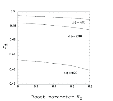
Figure 4: The numerically computed angular momentum of the black hole at different boosts for a black hole with mass $M=1$ and spin $a=1/2$. Three different resolutions $d\phi$ are shown.

A more realistic situation is to compute $J_{\Delta}$ and $M_{\Delta}$ during a numerical simulation of a black-hole spacetime, in which the spacetime data will be given on a spatial grid. To test our method in this case, we again use boosted Kerr-Schild data, but this time we start with numerical data discretized on a Cartesian mesh on a spatial slice; this mesh will not coincide with the spherical mesh on the apparent horizon. We use an apparent horizon finder to locate the apparent horizon $S$ and its unit spacelike normal $R^{a}$, and construct a spherical grid on the apparent horizon. Let $dx$ and $d\phi$ be the grid spacing of the Cartesian and spherical grid respectively. We want the two grids to be of similar spacing, i.e. we choose $d\phi$ such that $d\phi\approx dx/R$ where $R$ is the coordinate radius of the apparent horizon. The data are then interpolated onto the spherical grid, an additional source of error. We extract the two-metric $q_{ab}$ numerically from the data, use it to find the Killing vector field $\varphi^{a}$, and apply our formula for angular momentum. We present a series of test cases involving the black hole in boosted Kerr-Schild data. One is static, and three others have a spin of $1/2$ about the $z$-axis, with one of the spinning holes boosted perpendicular to the spin along the $x$-axis, another parallel to the spin along the $z$-axis. Table 1 lists the different scenarios.

Table 1: Various scenarios

Scenario	$M$	$a$	$v_{x}$	$v_{z}$
I	1	0	0	0
II	1	1/2	0	0
III	1	1/2	1/2	0
IV	1	1/2	0	1/2

Due to the additional complexity of having the data in a mesh that is not the one on $S$ where the calculation is done, we have to deal with two different numerical grids. We refined both the Cartesian grid and the spherical grid intrinsic to the apparent horizon to perform convergence tests. All runs were performed with three resolutions: 1. $dx=1/4$, $d\phi=10^{\circ}$; 2. $dx=1/8$, $d\phi=5^{\circ}$; 3. $dx=1/16$, $d\phi=2.5^{\circ}$. All lengths are measured in units of mass $M$ where $M$ is the mass of the black hole; $J_{\Delta}$ is measured in units of $M^{2}$. Figure 5 shows $J_{\Delta}$ versus resolution, and figure 6 displays $M_{\Delta}$ versus resolution, showing second-order convergence to the known solutions for each of the cases described in table 1.

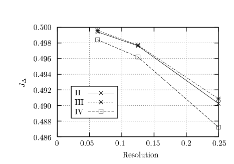
Figure 5: Resolution tests for the angular momentum $J_{\Delta}$ of the horizon. The scenarios II – IV are explained in table 1.

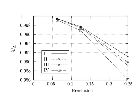
Figure 6: Resolution test for the mass $M_{\Delta}$ of the horizon. The scenarios II – IV are explained in table 1.

In addition to $J_{\Delta}$ and $M_{\Delta}$, we also monitor how well we converge to a truly isolated horizon, one in which the shear $\sigma$ is zero. Figure 7 plots the value of $\sigma$ versus resolution and demonstrates second-order convergence toward zero. As expected due to additional errors in the apparent horizon tracker, the convergence factors are not as good as in the case of analytic data; but are still acceptable for second order convergence.

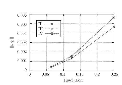
Figure 7: This graph shows the $L_{2}$ norm of $\sigma_{(\ell)}$. We see that it converges to zero, indicating that the horizon is isolated. The scenarios II – IV are explained in table 1.

V Discussion

In this section we want to compare our method of finding the mass and angular momentum of a black hole in a numerical simulation with other methods that are commonly used.

Note that the method proposed in this paper has three advantages: (i) it is not tied to a particular geometry (like the Kerr geometry), (ii) it is completely coordinate independent, and (iii) it only requires data that is intrinsic to the apparent horizon. The commonly used alternatives for calculating mass and angular momentum do not share all three of these features.

The reader might object to (i) on the grounds that our formula for $M_{\Delta}$ (equation (27)) is also motivated by the corresponding Kerr formula. In this regard, the following remarks are worth mentioning. Even though our formula for $M_{\Delta}$ is based on the corresponding Kerr equation, much less use is made of the specific properties of a Kerr black hole than in most conventional methods such as the great circle method described below. In particular, while deriving equation (27), we do not make any assumption regarding the near horizon geometry. All that is required is that the members of the Kerr family are elements of the phase space under consideration (see afk ; abl1 for a detailed specification of the phase space). The Kerr solutions are used only to provide a reference point for values of the black hole energy; this is somewhat analogous to choosing the zero of a potential in classical particle mechanics. In principle, we could also have chosen a different two parameter family of solutions but we choose the Kerr family due to its well known importance in black hole theory.

Owing to the uniqueness theorems of classical general relativity, it is commonly believed that a black hole that has been created in a violent event will radiate away all its higher multipole moments and settle down to form a Kerr black hole near the horizon. One strategy for assigning a mass and an angular momentum to a black hole is then to identify the member of the Kerr family one is dealing with and to read off the corresponding mass and angular momentum parameters.

While this strategy is physically well motivated, and one does expect the final black hole to be close to Kerr in some sense, we can refine this strategy considerably. The main difficulty with this method is that there are many subtleties and open questions regarding the issue of uniqueness of the final black hole. To briefly illustrate this point, let us consider the isolated horizon describing the final black hole. The intrinsic geometry of the horizon is, by definition, time independent. However, it is not necessary that four dimensional quantities evaluated at the horizon must also be time independent. For instance, using the Einstein equations at the isolated horizon, it turns out that the expansion and shear of the inward pointing normal $n^{a}$ (see equation (1)) may not be time independent; these quantities decay exponentially abl2 . This means that the four-geometry in the vicinity of a NEH is generically not time independent, and hence may not be isometric to a Kerr solution. It is also not clear whether the four geometry tends to the Kerr geometry as we approach future time like infinity. Clearly, we need to prove a statement which says: ‘sufficiently far’ into the future, the spacetime metric in a ‘sufficiently small’ neighborhood of the horizon, is ‘close to the Kerr metric’. In this statement, each phrase within quotes is ill defined. To prove or disprove such statements, it is imperative, at the very least, that one does not start with the assumption that the final black hole is Kerr. In particular, it is desirable that we not use geometrical properties of the Kerr horizon to calculate angular momentum and mass.

If one nevertheless makes the assumption that the final black hole is described by a Kerr geometry, one has to find a way to identify the particular member in the Kerr family. The method that is most commonly used is the great circle method which is based on properties of the Kerr horizon found by Smarr smarr . It can be described as follows:

In the usual coordinates, let $L_{e}$ be the proper length of the equator of the Kerr apparent horizon and $L_{p}$ the proper length of a polar meridian. Here the equator is the great circle of maximum length and a polar meridian is a great circle of minimum length. The distortion parameter $\delta$ is then defined to be $(L_{e}-L_{p})/L_{e}$. Smarr then showed that the knowledge of $\delta$, together with one other quantity like area, $L_{e}$, or $L_{p}$, is sufficient to find the parameters $m$ and $a$ of the Kerr geometry.

The difficulty with this method, apart from relying overly on properties of the Kerr spacetime, is that notions such as great circles, equator or polar meridian etc. are all highly coordinate dependent. If we represent the familiar two-metric on the Kerr horizon in different coordinates, the great circles in one coordinate system will not agree with great circles in the other system. The two coordinate systems will therefore give different answers for $M$ and $a$ as calculated by this method. In certain specific situations where one has a good intuition about the coordinate system being used and the physical situation being modelled, this method might be useful as a quick way of calculating angular momentum, but it is inadequate as a general method.

The problem of coordinate dependence can be dealt with in axisymmetric situations without assuming that the coordinate system used in the numerical code is adapted to the axial symmetry. The idea is to use the orbits of the Killing vector as analogs of the lines of latitude on a metric two-sphere. The analog of the equator is then the orbit of the Killing vector which has maximum proper length. This defines $L_{e}$ in an invariant way. The north and south poles are the points where the Killing vector vanishes, and the analog of $L_{p}$ is the length of a geodesic joining these two points (because of axial symmetry, all geodesics joining the poles will have the same length). Since this geodesic is necessarily perpendicular to the Killing vector, we just need to find the length of a curve which joins the north and south poles and is everywhere perpendicular to the Killing orbits. With $L_{e}$ and $L_{p}$ defined in this coordinate invariant way, we can follow the same procedure as in the great circle method to calculate the mass and angular momentum. This method can be called the generalized great circle method.

How does the generalized great circle method compare to our method? From a purely practical point of view, note that this method requires us to find the Killing vector, to determine the orbit of the Killing vector with maximum length, and to calculate the length of a curve joining the poles which is orthogonal to the Killing orbits. The first step is the same as in the isolated horizon method presented in this paper. While the next step in the isolated horizon method is simply to integrate a component of the extrinsic curvature on the horizon, this method requires more work, and furthermore, the numerical errors involved are at least as high as in the isolated horizon method. Thus the simplicity of the great circle method is lost when we try to make it coordinate invariant, and it retains the disadvantage of relying heavily on the properties of the Kerr geometry.

It should also be mentioned here that there exist exact solutions to Einstein’s equations representing static, non-rotating and axisymmetric black holes. Examples of such solutions are the distorted black hole solutions found by Geroch and Hartle gh or the solutions representing black holes immersed in electromagnetic fields ernst . The apparent horizons in all these solutions are distorted, and the generalized great circle method will give a non-zero value for the angular momentum. Our method based on equations (25) and (22) will give $J_{\Delta}=0$ because the imaginary part of $\Psi_{2}$ vanishes at the horizon for these solutions. While these solutions are probably not relevant for numerical simulations of binary black hole collisions, they represent physically interesting situations in which a black hole is surrounded by different kinds of external matter fields which distort the black hole; these black holes may have some relevance astrophysically. These solutions show that the generalized great circle method cannot be correct in general. They also illustrate that the great circle method will in general give results that are different from the ones obtained using Komar integrals.

A completely different approach to finding the mass and angular momentum of a black hole in a numerical solution is to use the concept of a Killing horizon. Since in a numerical simulation one is interested in highly dynamical situations, one can not assume the existence of Killing vectors in the whole spacetime. Instead one assumes that stationary and axial Killing vectors exist in a neighborhood of the horizon, and then uses appropriate Komar integrals to find the mass and angular momentum.

While this method is coordinate independent and does not rely on a specific metric, it has two disadvantages when compared with the isolated horizon approach. First, it is not a priori clear how the stationary Killing vector is to be normalized if it is only known in a neighborhood of the horizon. Secondly, this method requires the Killing vectors to be known in a whole neighborhood of the horizon. Computationally this is more expensive than finding a Killing vector just on the horizon. Conceptually it is also unclear how big this neighborhood of the horizon should be. Furthermore, at present there is no Hamiltonian framework available in which the boundary condition involves the existence of Killing vectors in a finite neighborhood of the horizon. In a sense, the isolated horizon framework extracts just the minimum amount of information from a Killing horizon in order to carry out the Hamiltonian analysis and define conserved quantities.

VI Applications and Future Directions

One situation where the calculation of $M_{\Delta}$ and $J_{\Delta}$ might be useful is in studying properties of initial data. Consider, for example, an initial data representing a binary black hole system. If the black holes are far apart, then we may consider them to be isolated (this can be verified, for example, by calculating the shear of the inward null normal as in equation (20)). Then the difference $E=M_{\Delta}^{1}+M_{\Delta}^{2}-M_{ADM}$ represents the binding energy between the holes plus the energy due to radiation and possibly also the kinetic energy of the black holes. In order to find the individual black hole masses $M_{\Delta}^{1}$ and $M_{\Delta}^{2}$ equations (25) and (27) will be useful for this purpose. It is also interesting to compare different initial data sets which represent roughly the same physical situation by calculating the quantity $E$. A lot of work in this direction has recently been carried out by Pfeiffer et al. pct . The isolated horizon framework may provide some further insights.

The isolated horizon framework may also be used to construct initial data representing two (or more) black holes far away from each other. We want to specify the individual black hole spins, velocities and masses in the initial data when the two black holes are very far apart. For this purpose, the formulae for $J_{\Delta}$ and $M_{\Delta}$ would be relevant, and we may assume that the black holes will be isolated at least for a short time and will form an isolated horizon. The isolated horizon conditions will then yield boundary conditions at the apparent horizon which can be used to solve the constraint equations on the spatial slice. In fact, pioneering work in this direction has already been carried out by Cook c ; the quasi-equilibrium boundary conditions developed by Cook are identical to the isolated horizon boundary conditions in many ways.

Let us also briefly discuss one more important future application: extracting radiation waveforms. We expect that information about gravitational radiation will be encoded in a component of the Weyl tensor such as $\Psi_{4}=C_{abcd}n^{a}\overline{m}^{b}n^{c}\overline{m}^{d}$ where $n^{a}$ and $m^{a}$ are members of a null tetrad. In certain situations where we have a background metric or if we have Killing vectors, there may be a natural choice of the null tetrad used to calculate $\Psi_{4}$. However, in general situations, it is not clear how to construct this preferred null tetrad. Without a well defined way of calculating radiation waveforms, it is very hard to even compare the results of different simulations which model similar physical situations but in different coordinates. It turns out that the isolated horizon framework could be used to provide a preferred coordinate system in the vicinity of an isolated horizon. For this purpose, we need more structure on the horizon than provided by a NEH; we need the notion of an isolated horizon as discussed briefly at the end of section II.1. It can be shown that, generically, an isolated horizon has a preferred foliation which may be said to define its rest frame. In general, this preferred foliation will not agree with the foliation given by the apparent horizons in a particular choice of Cauchy surfaces in spacetime. However, this preferred foliation can be constructed in a completely coordinate independent manner. Given this preferred foliation, we can construct a coordinate system analogous to the Bondi coordinates constructed near null infinity letter ; abl2 . This preferred coordinate provides an invariant way of calculating radiation waveforms and comparing the results of different simulations.

VII Acknowledgements

We would like to thank Abhay Ashtekar and Pablo Laguna for countless discussions, criticisms and suggestions. We are also grateful to Doug Arnold, Greg Cook, Harald Pfeiffer, and Jorge Pullin for useful discussions and suggestions. This work was supported in part by the NSF grants PHY01-14375, PHY-0090091 and PHY-9800973 and by the DFG grant SFB-382. BK was also supported by the Duncan Fellowship at Penn State. All the authors acknowledge the support of the Center for Gravitational Wave Physics, which is funded by the National Science Foundation under Cooperative Agreement PHY-0114375.

References

- (1) R. M. Wald and V. Iyer, Trapped Surfaces in the Schwarzschild Geometry and Cosmic Censorship, Phys. Rev.D44, R3719-R3722 (1991)
- (2) J. Thornburg, Finding Apparent Horizons in Numerical Relativity, Phys. Rev. D54, 4899 (1996).
- (3) T. Baumgarte, G. Cook, M. Sheel, S. Shapiro, and S. Teukolsky, Implementing an apparent-horizon finder in three dimensions, Phys. Rev. D54, 4849 (1996).
- (4) P. Anninos, K. Camarda, J. Libson, J. Masso, E. Seidel, and W.-M. Suen, Finding apparent horizons in dynamic 3D numerical spacetimes, Phys. Rev. D58, 024003 (1998).
- (5) M. F. Huq, M. W. Choptuik, and R. A. Matzner, Locating Boosted Kerr and Schwarzschild Apparent Horizons, gr-qc/0002076.
- (6) M. Alcubierre, S. Brandt, B. Bruegmann, C. Gundlach, J. Mosso, E. Seidel, and P. Walker, Test-beds and applications for apparent horizon finders in numerical relativity, Class. Quant. Grav. 17, 2159 (2000).
- (7) D. Shoemaker, M.Huq, R. Matzner, Generic Tracking of Multiple Apparent Horizons with Level Flow, Phys. Rev. D62, 124005 (2000).
- (8) E. Schnetter, A fast apparent horizon algorithm, gr-qc/0206003.
- (9) A. Ashtekar, C. Beetle, and S. Fairhurst, Mechanics of Isolated Horizons, Class. Quant. Grav. 17, 253 (2000).
- (10) A. Ashtekar, C. Beetle, O. Dreyer, S. Fairhurst, B. Krishnan, J. Lewandowski and J. Wisniewski, Generic Isolated Horizons and their Applications, Phys. Rev. Lett. 85, 3564-3567 (2000).
- (11) A. Ashtekar, S. Fairhurst, and B. Krishnan, Isolated Horizons: Hamiltonian Evolution and the First Law, Phys. Rev. D62 104025 (2000).
- (12) A. Ashtekar, C. Beetle, and J. Lewandowski, Mechanics of Rotating Isolated Horizons, Phys. Rev. D64, 044016 (2001).
- (13) A. Ashtekar, C. Beetle, and J. Lewandowski, Geometry of Generic Isolated Horizons, Class. Quant. Grav. 19, 1195–1225 (2002).
- (14) A. Ashtekar and B. Krishnan, Dynamical Horizons: Energy, Angular Momentum, Fluxes and Balance Laws, gr-qc/0207080.
- (15) S. W. Hawking and G. F. R. Ellis, The Large Scale Structure of Space-Time, Cambridge University Press (1975)
- (16) S. Hayward, General Laws of Black Hole Dynamics, Phys. Rev. D49, 6467-6474 (1994).
- (17) J. L. Friedman, K. Schleich, and D. M. Witt, Topological Censorship, Phys. Rev. Lett. 71, 1486-1489 (1993).
- (18) R. Geroch and J. B. Hartle, Distorted Black Holes, J. Math. Phys. 23(4) 680 (1982).
- (19) J. Stewart, Advanced General Relativity, Cambridge University Press (1991).
- (20) R. M. Wald, General Relativity, University of Chicago Press (1984).
- (21) A. Ashtekar and A. Magnon-Ashtekar, A technique for analyzing the structure of isometries, J. Math. Phys. 19(7), 1567-1572 (1978).
- (22) R. A. Matzner, M. F. Huq, and D. Shoemaker, Initial Data and Coordinates for Multiple Black Hole Systems, Physical Review D59, 024015 (1999).
- (23) S. Chandrasekhar, Mathematical Theory of Black Holes, Oxford Classic Texts in the Physical Sciences (1998)
- (24) L. Smarr, Surface Geometry of Charged Rotating Black Holes, Phys. Rev. D7, 289-295 (1973).
- (25) F. J. Ernst, Black Holes in a Magnetic Universe, J. Math. Phys. 17, 54-56 (1976).
- (26) H. P. Pfeiffer, G. B. Cook, and S. A. Teukolsky, Comparing Initial Data Sets for Binary Black Holes, Phys. Rev. D66, 024047 (2002).
- (27) G. B. Cook, Corotating and Irrotational Binary Black Holes in Quasi-Circular Orbits, Phys. Rev. D65, 084003 (2002).