Dynamical mass ejection from black hole-neutron star binaries

Abstract

We investigate properties of material ejected dynamically in the merger of black hole-neutron star binaries by numerical-relativity simulations. We systematically study the dependence of ejecta properties on the mass ratio of the binary, spin of the black hole, and equation of state of the neutron-star matter. Dynamical mass ejection is driven primarily by tidal torque, and the ejecta is much more anisotropic than that from binary neutron star mergers. In particular, the dynamical ejecta is concentrated around the orbital plane with a half opening angle of $10\mathrm{°}$–$20\mathrm{°}$ and often sweeps out only a half of the plane. The ejecta mass can be as large as $\sim 0.1M_{\odot}$, and the velocity is subrelativistic with $\sim 0.2$–$0.3c$ for typical cases. The ratio of the ejecta mass to the bound mass (disk and fallback components) is larger, and the ejecta velocity is larger, for larger values of the binary mass ratio, i.e., for larger values of the black-hole mass. The remnant black hole-disk system receives a kick velocity of $O(100)$ $\mathrm{km}\text{\,}{\mathrm{s}}^{-1}$ due to the ejecta linear momentum, and this easily dominates the kick velocity due to gravitational radiation. Structures of postmerger material, velocity distribution of the dynamical ejecta, fallback rates, and gravitational waves are also investigated. We also discuss the effect of ejecta anisotropy on electromagnetic counterparts, specifically a macronova/kilonova and synchrotron radio emission, developing analytic models.

I Introduction

Coalescences of black hole-neutron star binaries are one of the most promising gravitational-wave sources for ground-based laser-interferometric detectors Harry and LIGO Scientific Collaboration (2010); F. Acernese et al. (2015); Somiya (2012), along with those of binary neutron stars and binary black holes. The sensitivity of these detectors will reach a sufficiently high level in the coming years to detect gravitational waves from compact binary coalescences more often than once a year J. Abadie et al. (2010); Dominik et al. (2015). The first direct detection of gravitational waves must have a dramatic impact on fundamental physics. Furthermore, gravitational waves from binaries involving neutron stars will tell us neutron-star properties like the radius, compactness, and tidal deformability. Knowledge of neutron-star properties will allow us to constrain the equation of state of nuclear- and supranuclear-density matter, and therefore gravitational waves will also give us valuable information on nuclear physics.

Simultaneous detection of electromagnetic radiation from compact binary mergers, i.e., electromagnetic counterparts to gravitational waves, is eagerly desired Metzger and Berger (2012); Piran et al. (2013). It will support gravitational-wave detection and enhance scientific returns from each coalescence event. For example, source localization on the celestial sphere is much more accurate with electromagnetic instruments than with gravitational-wave detector networks Nissanke et al. (2013). Gravitational-wave data analysis benefits from accurate localization by solving degeneracy between the sky location and other amplitude parameters such as the luminosity distance. Accurate localization of the source is also indispensable to find its host galaxy and to determine the cosmological redshift. By combining this information, the luminosity distance-redshift relation will be derived without relying on the cosmic distance ladder, and we will obtain a novel method to test cosmological models Schutz (1986). Besides, the effective sensitivity of a gravitational-wave detector would be improved if we could know the coalescence time and/or sky location of a binary from electromagnetic counterparts Kochanek and Piran (1993).

Among the candidates of electromagnetic counterparts, a short-hard gamma-ray burst and its afterglow are vigorously studied both theoretically and observationally (see Refs. Nakar (2007); Berger (2014) for reviews). While whether compact binary coalescences can really drive short-hard gamma-ray bursts is still an open question, future simultaneous detection with gravitational-wave chirp signals will prove this hypothesis. Prompt emission is so bright that it can be easily detected by gamma-ray satellites within the horizon distance of gravitational-wave detectors. Accurate localization is possible if an associated afterglow is observed at longer wavelengths. Short-hard gamma-ray bursts do not, however, always serve as counterparts to gravitational waves because of their presumably jetlike geometry. If the typical jet opening angle is $\lesssim$$$ as suggested by jet-break observations W. Fong et al. (2012, 2014), the fraction of gravitational-wave events accompanied by observable short-hard gamma-ray bursts will be a few percent at best.

In recent years, electromagnetic counterparts have been getting a lot more attention, and many isotropic emission models are studied. Most of the proposed models require the ejection of unbound material from the binary, where examples include a macronova/kilonova powered by decay heat of unstable r-process elements Li and Paczyński (1998); Kulkarni ; Metzger et al. (2010a); Kisaka et al. (2015) and nonthermal radiation from electrons accelerated at blast waves between the ejecta and interstellar medium Nakar and Piran (2011); Takami et al. (2014a). Possible emission from the ejecta will be isotropic if the ejecta has spherical geometry and/or a subrelativistic velocity. Such a “$4\pi$-counterpart” is ideal for followup observations, because it will accompany a majority of gravitational-wave events unlike beamed radiation of short-hard gamma-ray bursts.

Despite its 40-years-old history in theoretical astrophysics Lattimer and Schramm (1974, 1976), mass ejection from the compact binary merger is a young research topic in numerical relativity. Most of the previous black hole-neutron star binary simulations in numerical relativity were performed aiming at deriving gravitational waves in the late inspiral and merger phases and at clarifying properties of remnant accretion disks formed after the tidal disruption of neutron stars (see Ref. Shibata and Taniguchi (2011) and references therein for earlier work). Mass ejection has not been studied in detail compared to these topics in full general relativity Kyutoku et al. (2011a); Foucart et al. (2013a); Lovelace et al. (2013); Deaton et al. (2013); Foucart et al. (2014), whereas a substantial effort to clarify mass ejection has been made in simulations performed in Newtonian gravity or approximate general relativity Rosswog (2005); Rosswog et al. (2013); Just et al. (2015) (see also Refs. Lee and Kluźniak (1999); Lee (2000, 2001); Faber et al. (2006a, b); Rantsiou et al. (2008); Ruffert and Janka (2010)). It is pointed out that dynamical ejecta from binary neutron star mergers become less massive and more isotropic in full general relativity Hotokezaka et al. (2013a) or the conformal flatness approximation Bauswein et al. (2013) than in Newtonian gravity Rosswog et al. (1999, 2000, 2013). The difference due to realism of the gravity should be most pronounced when a black hole is involved as already suggested by existing work. Thus, it is natural that numerical relativity is vital to study mass ejection from the black hole-neutron star binary merger.

In this study, we perform simulations of black hole-neutron star binary mergers using numerical-relativity code SACRA Yamamoto et al. (2008) and investigate dynamical mass ejection extending our preceding work Kyutoku et al. (2013). In particular, we focus on kinematical properties of dynamical ejecta such as the mass and velocity. Compared to our previous simulations Kyutoku et al. (2011a), we adopt large computational domains to track long-term evolution of the ejecta. Because the dynamical ejecta has a velocity comparable (a few tens of percent) to the speed of light as shown in this study, the large computational domains are essential for the reliable estimation of ejecta properties. We also improve the treatment of artificial atmosphere (inevitable in conservative hydrodynamic schemes) from our previous work Shibata et al. (2009); Yamamoto et al. (2008); Shibata et al. (2012); Kyutoku et al. (2010, 2011b, 2011a) and confirm that characteristic quantities of dynamical ejecta such as the mass and velocity depend only weakly on the atmosphere. We do not, however, study disk winds expected to be driven by unincorporated physics.

This paper is organized as follows. Section II describes our models of black hole-neutron star binaries including neutron-star equations of state. Our numerical methods are also described, and diagnostics of simulations are presented with particular emphasis on the ejecta defined as unbound material. Numerical results of the simulations are presented in Sec. III. After briefly reviewing the merger dynamics in Sec. III.1, dynamical mass ejection processes are described in Sec. III.2. The dependence of characteristic quantities on binary parameters is discussed in Sec. III.3, and the material structure is investigated in Sec. III.4. We also study fallback material, remnant black hole-disk systems, and gravitational waves in Secs. III.5, III.6, and III.7, respectively. Possible electromagnetic counterparts from black hole-neutron star binaries are discussed based on the results of simulations in Sec. IV. Specifically, Sec. IV.1 describes the macronova/kilonova and Sec. IV.2 describes synchrotron radio emission from accelerated electrons. Section V is devoted to a summary. Numerical values of characteristic ejecta quantities derived by simulations are summarized in Table 3. Readers interested primarily in electromagnetic counterparts should read Sec. IV, of which important results are described in Ref. Kyutoku et al. (2013).

Notational conventions are summarized as follows. Throughout this paper, we adopt geometrical units in which $G=c=1$, where $G$ and $c$ are the gravitational constant and speed of light, respectively. Exceptionally, $c$ is sometimes inserted for clarity when we discuss the velocity of the ejecta or fluid element. Greek and Latin indices denote the spacetime and space components, respectively. The black-hole mass, neutron-star gravitational mass, and neutron-star circumferential radius in isolation are denoted by $M_{\mathrm{BH}}$, $M_{\mathrm{NS}}$, and $R_{\mathrm{NS}}$, respectively. The dimensionless spin parameter of the black hole, total mass of the system at an infinite separation, mass ratio, and compactness of the neutron star are defined as $\chi\equiv S_{\mathrm{BH}}/M_{\mathrm{BH}}^{2}$, $m_{0}\equiv M_{\mathrm{BH}}+M_{\mathrm{NS}}$, $Q\equiv M_{\mathrm{BH}}/M_{\mathrm{NS}}$, and $\mathcal{C}\equiv M_{\mathrm{NS}}/R_{\mathrm{NS}}$, respectively, where $S_{\mathrm{BH}}$ is the black-hole spin angular momentum.

II Numerical method

II.1 Zero-temperature equation of state

Table 1: Parameters and key ingredients of the adopted equations of state, where $P_{2}$ (the pressure at $\rho=$e14.7\text{\,}\mathrm{g}\text{\,}{\mathrm{cm}}^{-3}$$) is shown in units of $\mathrm{d}\mathrm{y}\mathrm{n}\mathrm{e}\,\mathrm{c}\mathrm{m}^{-2}$. $M_{\mathrm{max}}$ is the maximum gravitational mass of a spherical neutron star for a given equation of state. $R_{1.35}$, $\rho_{1.35}$, $M_{*,1.35}$, $\mathcal{C}_{1.35}$, $k_{1.35}$, and $\Lambda_{1.35}$ are the circumferential radius, central rest-mass density, baryon rest mass, compactness, quadrupolar tidal Love number, and dimensionless quadrupolar tidal deformability of a $1.35M_{\odot}$ neutron star, respectively.

Model	$\log_{10}(P_{2})$	$\Gamma_{1}$	$\Gamma_{2}$	$\Gamma_{3}$	$M_{\mathrm{max}}[M_{\odot}]$	$R_{1.35}$ ($\mathrm{km}$)	$\rho_{1.35}$ ($\mathrm{g}\text{\,}{\mathrm{cm}}^{-3}$)	$M_{*,1.35}[M_{\odot}]$	$\mathcal{C}_{1.35}$	$k_{1.35}$	$\Lambda_{1.35}$
APR4	34.269	2.830	3.445	3.348	2.20	11.1	$8.9\text{\times}{10}^{14}$	1.50	0.180	0.0908	323
ALF2	34.616	4.070	2.411	1.890	1.99	12.4	$6.4\text{\times}{10}^{14}$	1.49	0.161	0.120	734
H4	34.669	2.909	2.246	2.144	2.03	13.6	$5.5\text{\times}{10}^{14}$	1.47	0.147	0.115	1110
MS1	34.858	3.224	3.033	1.325	2.77	14.4	$4.2\text{\times}{10}^{14}$	1.46	0.138	0.132	1740

We model equations of state of zero-temperature neutron-star matter by piecewise polytropes Read et al. (2009). Neutron stars in compact binaries right before the merger will be cold enough to be modeled by zero-temperature equations of state (see, e.g., Ref. Yakovlev and Pethick (2004)). However, the realistic equation of state of neutron-star matter is not known precisely yet. Therefore, it is necessary to adopt various equations of state systematically to span a plausible range of neutron-star properties. Piecewise polytropes are suitable for this purpose, because those with one and three pieces for crust and core regions, respectively, are known to be able to approximate nuclear-theory-based equations of state accurately with a small number of parameters Read et al. (2009). Following Ref. Read et al. (2009), we employ piecewise polytropes of the form

$$P(\rho)=\kappa_{i}\rho^{\Gamma_{i}}\;(\rho_{i}\leq\rho\leq\rho_{i+1}),$$ (1)

where $P$ is the pressure and $\rho$ is the rest-mass density, with $i\in\{0,1,2,3\}$ in this study. It is always assumed that $\rho_{0}=0$ and $\rho_{4}\to\infty$. We fix parameters for the lowest-density, crust region to be

$$\Gamma_{0} =$1.356\,923\,95$,$$ (2)

$$\kappa_{0} =$3.998\,736\,92\text{\times}{10}^{-8}\text{\,}\mathrm{(}\mathrm{g}~{}\mathrm{c}\mathrm{m}^{-3}\mathrm{)}$^{1-\Gamma_{0}}.$$ (3)

We further set $\rho_{2}=$e14.7\text{\,}\mathrm{g}\text{\,}{\mathrm{cm}}^{-3}$\approx$5.0\text{\times}{10}^{14}\text{\,}\mathrm{g}\text{\,}{\mathrm{cm}}^{-3}$$ and $\rho_{3}=$e15.0\text{\,}\mathrm{g}\text{\,}{\mathrm{cm}}^{-3}$$ to reduce the number of free parameters. Requiring the continuity of $P(\rho)$, each piecewise polytrope is characterized by four parameters. We choose the free parameters to be the pressure at $\rho_{2}$, denoted by $P_{2}=P(\rho_{2})$, and adiabatic indices for the core, $\{\Gamma_{1},\Gamma_{2},\Gamma_{3}\}$.

Table 1 lists parameters of piecewise polytropes adopted in this study as well as neutron-star properties computed using them. The naming convention and parameters follow Ref. Read et al. (2009). APR4 Akmal et al. (1998) is computed by a variational method incorporating three-nucleon interactions and relativistic boost corrections. This equation of state gives the smallest radius of a $1.35M_{\odot}$ neutron star, $R_{1.35}=$11.1\text{\,}\mathrm{km}$$, and thus APR4 is the softest equation of state among those adopted in this study. Accordingly, tidal disruption is less pronounced for neutron stars modeled with APR4 than those modeled with the other equations of state. ALF2 Alford et al. (2005) is a hybrid equation of state obtained combining a nucleonic, APR-type equation of state at low density and a quark-matter equation of state with quantum chromodynamics corrections at high density. H4 Glendenning and Moszkowski (1991); Lackey et al. (2006) is computed by relativistic mean-field theory incorporating hyperons with the stiffest possible parameters (at the time). MS1 Müller and Serot (1996) is also derived by relativistic mean-field theory for nucleonic matter and gives $R_{1.35}=$14.4\text{\,}\mathrm{km}$$, which is the largest value in this study. Thus, MS1 is an extreme example with which tidal disruption occurs most violently.

In practice, a very-high-density regime is not relevant to black hole-neutron star binary coalescences as far as canonical-mass neutron stars with $M_{\mathrm{NS}}\approx 1.35M_{\odot}$ Özel et al. (2012); Lattimer (2012) are concerned. The reason for this is that the maximum rest-mass density of the system, i.e., the central density of the neutron star and maximum density in the remnant accretion disk, is a decreasing function of time except for subdominant oscillations. The rest-mass density at the center of an isolated $1.35M_{\odot}$ neutron star, $\rho_{1.35}$, never exceeds $\rho_{3}$ for the equations of state adopted in this study (see Table 1), and hence $\Gamma_{3}$ never plays a role in black hole-neutron star binary coalescences. For MS1, even $\Gamma_{2}$ is irrelevant, because $\rho_{1.35}$ is lower than $\rho_{2}$. This situation is in stark contrast to that of binary neutron star coalescences, which depend crucially on the high-density regime of the equations of state.

In this study, we regard quantities associated with $1.35M_{\odot}$ neutron stars as characteristic quantities of the equation of state rather than the maximum mass $M_{\mathrm{max}}$, which is sensitive to the behavior of matter at high density. Table 1 shows the baryon rest mass $M_{*}$, compactness $\mathcal{C}$, quadrupolar tidal Love number $k$ Hinderer (2008, 2009), and dimensionless quadrupolar tidal deformability $\Lambda\equiv(2/3)k\mathcal{C}^{-5}$ of a $1.35M_{\odot}$ neutron star, in addition to $R_{1.35}$, $\rho_{1,35}$, and $M_{\mathrm{max}}$. Note that all the equations of state can support $\sim 2M_{\odot}$ neutron stars and satisfy constraints from observations of massive pulsars Demorest et al. (2010); J. Antoniadis et al. (2013), and thus they are possible candidates of the realistic equation of state.

II.2 Initial condition

We adopt quasiequilibrium states of black hole-neutron star binaries as initial data of our simulations in the same manner as Refs. Kyutoku et al. (2010, 2011b, 2011a). Here, we briefly describe the computational method of quasiequilibrium states, and the details are found in Refs. Kyutoku et al. (2009, 2011a). Numerical computations are performed using the multidomain spectral method library LORENE LORENE website .

We solve a subset of the Einstein equation and the hydrostatic equilibrium equations assuming the existence of helical symmetry. Hamiltonian and momentum constraints are solved by a mixture of the conformal transverse-traceless decomposition York (1979) and extended conformal thin-sandwich formulation York (1999); Pfeiffer and York (2003) imposing the spatial conformal flatness, maximal slicing, and preservation of them in time. The singularity associated with the black hole is handled in the puncture framework Brandt and Brügmann (1997), and thus we obtain initial data of the induced metric $\gamma_{ij}$ and extrinsic curvature $K_{ij}$ everywhere on the initial hypersurface (except for the exact location of the puncture, with which simulation grids are chosen not to coincide). The neutron-star matter is modeled by a perfect fluid expressed by an energy-momentum tensor of the form

$$T_{\mu\nu}=\rho hu_{\mu}u_{\nu}+Pg_{\mu\nu},$$ (4)

where $h\equiv 1+\varepsilon+(P/\rho)$ is the specific enthalpy, $\varepsilon$ is the specific internal energy, and $u^{\mu}$ is the fluid four-velocity. We further assume that the fluid is in a zero-temperature and irrotational state during the computation of the initial data, and hydrostatic equilibrium configurations are obtained by solving the continuity equation and local energy-momentum conservation equation Bonazzola et al. (1997); Asada (1998); Teukolsky (1998); Shibata (1998).

Parameters characterizing a black hole-neutron star binary are specified in initial data computations (see Refs. Kyutoku et al. (2009, 2011a) for the details). For simplicity, we always choose $M_{\mathrm{NS}}$ to be a typical mass of observed binary neutron stars, $M_{\mathrm{NS}}=1.35M_{\odot}$, in this study Özel et al. (2012); Lattimer (2012). With this choice, the black-hole mass, $M_{\mathrm{BH}}$, is uniquely determined by the mass ratio, $Q$, which we regard as an independent parameter instead of $M_{\mathrm{BH}}$ itself. We only consider cases in which the spin angular momentum of the black hole is zero or aligned with the orbital angular momentum of the binary, and thus the spin is fully characterized by its dimensionless magnitude, $\chi$. The orbital angular velocity of a binary $\Omega$ is determined by a force-balance condition at the center of the neutron star for a given orbital separation. We use a dimensionless orbital angular velocity $m_{0}\Omega$ to characterize the initial data rather than the orbital separation.

II.3 Dynamical simulation

Our numerical simulations are performed using an adaptive-mesh-refinement code, SACRA Yamamoto et al. (2008). The Einstein evolution equations are solved in a Baumgarte–Shapiro–Shibata–Nakamura formulation Shibata and Nakamura (1995); Baumgarte and Shapiro (1998). We evolve the conformal-factor variable $W$, conformal metric $\tilde{\gamma}_{ij}$, conformal connection function $\tilde{\Gamma}^{i}$, extrinsic curvature trace $K$, and conformally weighted traceless part of the extrinsic curvature $\tilde{A}_{ij}$ defined by

$$W \equiv\gamma^{-1/6}\;,\;\tilde{\gamma}_{ij}\equiv\gamma^{-1/3}\gamma_{ij}\;,\;\tilde{\Gamma}^{i}\equiv-\partial_{j}\tilde{\gamma}^{ij},$$ (5)

$$K \equiv K_{ij}\gamma^{ij}\;,\;\tilde{A}_{ij}\equiv\gamma^{-1/3}\left(K_{ij}-\frac{1}{3}K\gamma_{ij}\right),$$ (6)

where Cartesian coordinates are adopted. The lapse function $\alpha$ and shift vector $\beta^{i}$ are evolved by a moving puncture gauge condition Campanelli et al. (2006); Baker et al. (2006) of the form

$$\left(\partial_{t}-\beta^{j}\partial_{j}\right)\alpha =-2\alpha K,$$ (7)

$$\left(\partial_{t}-\beta^{j}\partial_{j}\right)\beta^{i} =\frac{3}{4}B^{i},$$ (8)

$$\left(\partial_{t}-\beta^{j}\partial_{j}\right)B^{i} =\left(\partial_{t}-\beta^{j}\partial_{j}\right)\tilde{\Gamma}^{i}-\eta_{s}B^{i},$$ (9)

where $B^{i}$ is an auxiliary vectorial variable and $\eta_{s}$ is a free parameter. Initial data of the lapse function are given by $\alpha=W$, and the shift vector is initialized as $\beta^{i}=0$ with $B^{i}=0$. We adopt $\eta_{s}\approx 1/m_{0}$ in this study.

Hydrodynamic evolution equations are solved by a high-resolution shock-capturing central scheme Kurganov and Tadmor (2000) with third-order piecewise parabolic reconstruction Colella and Woodward (1984). We evolve the conserved rest-mass density $\rho_{*}$, conserved momentum density $\rho_{*}\hat{u}_{i}$, and conserved energy density $\rho_{*}\hat{e}$ defined via

$$\rho_{*}\equiv\rho\alpha\sqrt{\gamma}u^{t}\;,\;\hat{u}_{i}\equiv hu_{i}\;,\;\hat{e}\equiv h\alpha u^{t}-\frac{P}{\rho\alpha u^{t}}.$$ (10)

Equations of state adopted in dynamical simulations comprise cold and thermal parts. The former is taken to be piecewise polytropes described in Sec. II.1, and the latter is given by an ideal-gas-like form

$$P_{\mathrm{th}}=(\Gamma_{\mathrm{th}}-1)\rho\varepsilon_{\mathrm{th}},$$ (11)

where the thermal-part specific internal energy is defined by $\varepsilon_{\mathrm{th}}(\rho,\varepsilon)\equiv\varepsilon-\varepsilon_{\mathrm{cold}}(\rho)$ with $\varepsilon_{\mathrm{cold}}(\rho)$ the cold-part specific internal energy computed by piecewise polytropes. Total pressure is given by $P=P_{\mathrm{cold}}(\rho)+P_{\mathrm{th}}(\rho,\varepsilon)$, where $P_{\mathrm{cold}}(\rho)$ is computed by piecewise polytropes. We choose a fiducial value of $\Gamma_{\mathrm{th}}$ to be 1.8 following Ref. Hotokezaka et al. (2013a) (see also Ref. Bauswein et al. (2010)) and also adopt 1.6 and 2.0 for selected models (see Appendix A.3). Note that these values are larger than that adopted in our previous work Kyutoku et al. (2010, 2011b, 2011a), in which $\Gamma_{\mathrm{th}}$ is always chosen to be $\Gamma_{0}$ [see Eq. (2)].

In our simulations, all the postmerger material is governed effectively by the same sub-nuclear-density equation of state irrespective of the adopted piecewise polytrope. Specifically, when the rest-mass density falls below $\rho_{1}$, the equation of state is given by the sum of the crust polytrope and thermal correction,

$$P(\rho<\rho_{1},\varepsilon)=\kappa_{0}\rho^{\Gamma_{0}}+(\Gamma_{\mathrm{th}}-1)\rho\varepsilon_{\mathrm{th}}.$$ (12)

The values of $\rho_{1}$ are computed as $(\kappa_{0}\rho_{2}^{\Gamma_{1}}/P_{2})^{1/(\Gamma_{1}-\Gamma_{0})}$ for each piecewise polytrope (see Sec. II.1) and take 0.9–$2\text{\times}{10}^{14}\text{\,}\mathrm{g}\text{\,}{\mathrm{cm}}^{-3}$. The rest-mass density never exceeds these values after tidal disruption of neutron stars.

An artificial atmosphere has to be set carefully to study mass ejection accurately. According to Ref. Hotokezaka et al. (2013a), we put an atmospheric density floor of the form

$$\rho_{*,\mathrm{at}}=f_{\mathrm{at}}\rho_{*,0}\;\mathrm{min}\left[1,\left(\frac{R_{\mathrm{crit}}}{r}\right)^{n_{\mathrm{at}}}\right],$$ (13)

where $\rho_{*,0}$ is the maximum (conserved) rest-mass density of the initial configuration (see Ref. Yamamoto et al. (2008) for our previous treatment). We typically choose $f_{\mathrm{at}}=${10}^{-12}$$ and $n_{\mathrm{at}}=3$ and vary them for selected models (see Appendix A.2). The critical radius $R_{\mathrm{crit}}$ is chosen to be $L/16$, where $L$ is the size of the computational domain on one side (see below). The atmospheric velocity is set to be zero, and the atmospheric pressure is given by zero-temperature equations of state.

The grid structure of SACRA is summarized as follows. Computational domains are composed of nested equidistant Cartesian grids, and each grid has $(2N+1,2N+1,N+1)$ points in $(x,y,z)$ directions. The equatorial symmetry is imposed on the $z=0$ plane. We adopt $N=60$ as a fiducial value, with which the neutron-star radius is covered by $\gtrsim 50$ points in the finest grid. We also perform simulations with $N=40$ and 48 for selected models to check the convergence of ejecta properties (see Appendix A.1). The outer boundary is a cuboid covering $(x,y,z)\in[-L:L]\times[-L:L]\times[0:L]$, and outgoing-wave boundary conditions are imposed except for the $z=0$ plane. As for the adaptive-mesh-refinement grid structure, we prepare $l_{c}$ coarser nonmoving grids and $l_{f}$ finer moving grids. Namely, we have $l_{c}+2l_{f}$ computational grids spanning $l_{c}+l_{f}$ refinement levels, which we always choose to be 9 in this study. The nonmoving grids are fixed around an approximate center of mass throughout the simulation. One set of the moving grids follows the black hole, and the other set follows the neutron star. Starting from the coarsest level as $l=0$, the $l$th level has a grid spacing $\Delta x_{l}\equiv L/(2^{l}N)$, and we specifically denote the grid spacing at the finest level by $\Delta x\equiv L/(2^{l_{c}+l_{f}-1}N)$. Finally, time steps of all the moving grids are chosen by setting the Courant–Friedrichs–Lewy factor to be 0.5, and those of the nonmoving grids are chosen to agree with that of the $l_{c}$th level (i.e., the coarsest moving grid). In other words, the Courant–Friedrichs–Lewy factor is given by $0.5/2^{l_{c}-l}$ in the nonmoving grids.

II.4 Binary model and grid setting

Table 2: Key parameters of initial data and grid structures of simulations for models adopted in this study. The names of models represent the equation of state (EOS), mass ratio ($Q$), and dimensionless spin parameter of the black hole ($\chi$). $m_{0}\Omega_{0}$, $M_{0}$, and $J_{0}$ are the dimensionless initial orbital angular velocity, Arnowitt–Deser–Misner mass, and orbital angular momentum of the system, respectively. As for grid configurations, $l_{c}$ and $l_{f}$ are the numbers of coarser nonmoving grids and of a half of finer moving grids, respectively. The grid spacing at the finest level for $N=60$ (fiducial resolution) is shown in physical units as well as a value normalized by $m_{0}\approx 2(Q+1)$ km. The grid number assigned to the semimajor diameter of the neutron star is given by $R_{\mathrm{diam}}/\Delta x$ for the direction along the binary separation. The box size $L$ is shown in physical units as well as a value normalized by the initial gravitational wavelength $\lambda_{0}=\Omega_{0}/\pi$.

Model	EOS	$Q$	$\chi$	$m_{0}\Omega_{0}$	$M_{0}[M_{\odot}]$	$J_{0}[M_{\odot}^{2}]$	$l_{c}$	$l_{f}$	$\Delta x$ ($\mathrm{m}$)	$\Delta x/m_{0}$	$R_{\mathrm{diam}}/\Delta x$	$L$ ($\mathrm{km}$)	$L/\lambda_{0}$
APR4-Q3a75	APR4	3	0.75	0.036	5.35	18.74	5	4	162	0.0203	102	2486	3.6
ALF2-Q3a75	ALF2	3	0.75	0.036	5.35	18.74	5	4	186	0.0233	102	2858	4.1
H4-Q3a75	H4	3	0.75	0.036	5.35	18.74	5	4	209	0.0263	102	3215	4.6
MS1-Q3a75	MS1	3	0.75	0.036	5.35	18.74	5	4	228	0.0286	101	3501	5.0
APR4-Q3a5	APR4	3	0.5	0.036	5.35	19.15	5	4	162	0.0203	102	2486	3.6
ALF2-Q3a5	ALF2	3	0.5	0.036	5.35	19.15	5	4	186	0.0233	102	2858	4.1
H4-Q3a5	H4	3	0.5	0.036	5.35	19.15	5	4	209	0.0263	102	3215	4.6
MS1-Q3a5	MS1	3	0.5	0.036	5.35	19.15	5	4	228	0.0286	101	3501	5.0
APR4-Q3a0	APR4	3	0	0.036	5.35	19.98	5	4	162	0.0203	102	2486	3.6
ALF2-Q3a0	ALF2	3	0	0.036	5.35	19.98	5	4	186	0.0233	102	2858	4.1
H4-Q3a0	H4	3	0	0.036	5.35	19.98	5	4	209	0.0263	102	3215	4.6
MS1-Q3a0	MS1	3	0	0.036	5.35	19.98	5	4	228	0.0286	101	3501	5.0
APR4-Q5a75	APR4	5	0.75	0.040	8.04	30.13	4	5	158	0.0132	102	2429	2.6
ALF2-Q5a75	ALF2	5	0.75	0.040	8.04	30.13	4	5	181	0.0152	102	2786	3.0
H4-Q5a75	H4	5	0.75	0.040	8.04	30.13	4	5	205	0.0171	101	3144	3.3
MS1-Q5a75	MS1	5	0.75	0.040	8.04	30.13	4	5	219	0.0183	102	3358	3.6
APR4-Q5a5	APR4	5	0.5	0.040	8.04	30.99	4	5	158	0.0132	102	2429	2.6
ALF2-Q5a5	ALF2	5	0.5	0.040	8.04	30.99	4	5	181	0.0152	102	2786	3.0
H4-Q5a5	H4	5	0.5	0.040	8.04	30.99	4	5	205	0.0171	101	3144	3.3
MS1-Q5a5	MS1	5	0.5	0.040	8.04	30.99	4	5	219	0.0183	102	3358	3.6
APR4-Q7a75	APR4	7	0.75	0.044	10.73	40.96	4	5	153	0.0096	103	2358	2.1
ALF2-Q7a75	ALF2	7	0.75	0.044	10.73	40.96	4	5	179	0.0112	101	2751	2.4
H4-Q7a75	H4	7	0.75	0.044	10.73	40.96	4	5	200	0.0125	102	3072	2.7
MS1-Q7a75	MS1	7	0.75	0.044	10.73	40.96	4	5	215	0.0135	102	3301	2.9
APR4-Q7a5	APR4	7	0.5	0.044	10.73	42.35	4	5	154	0.0097	102	2372	2.1
ALF2-Q7a5	ALF2	7	0.5	0.044	10.73	42.35	4	5	179	0.0112	102	2743	2.4
H4-Q7a5	H4	7	0.5	0.044	10.74	42.35	4	5	201	0.0126	101	3086	2.7
MS1-Q7a5	MS1	7	0.5	0.044	10.74	42.35	4	5	217	0.0136	101	3329	2.9

Table 2 lists black hole-neutron star binary models considered in this study. We name each model after the equation of state, mass ratio, and black-hole spin. For example, APR4-Q3a75 is a binary modeled with the APR4 equation of state, $Q=3$, and $\chi=0.75$. Recall that $M_{\mathrm{NS}}=1.35M_{\odot}$ for all the models. Table 2 also presents the dimensionless initial orbital angular velocity $m_{0}\Omega_{0}$, Arnowitt–Deser–Misner mass $M_{0}$, and orbital angular momentum of the system $J_{0}$. Here, $J_{0}$ is defined from an Arnowitt–Deser–Misner type integral by subtracting the spin angular momentum associated with the puncture.

We take the mass ratio, $Q$, from $\{3,5,7\}$, and the dimensionless spin parameter, $\chi$, from $\{0.75,0.5,0\}$, where the spins are always prograde, i.e., parallel to the orbital angular momentum. Currently, neither the typical mass nor the typical spin of stellar-mass black holes is known from observations. Thus, we perform simulations systematically adopting various values of them along with equations of state to predict possible outcomes of binary mergers. Here, $Q=3,5$, and 7 correspond to $M_{\mathrm{BH}}=4.05M_{\odot}$, $6.75M_{\odot}$, and $9.45M_{\odot}$, respectively. The low-mass black hole with $\approx 4M_{\odot}$ is consistent with an observation of a black hole-Be star binary Casares et al. (2014), which could evolve into a black hole-neutron star binary, whereas the existence of a mass gap around 3–$5M_{\odot}$ is frequently debated Özel et al. (2010); Kreidberg et al. (2012). The middle-mass, $\approx 7M_{\odot}$, and massive, $\approx 10M_{\odot}$, black holes are safely expected to exist from observations of x-ray binaries Özel et al. (2010); Kreidberg et al. (2012). The spin parameter is even less constrained than the mass is McClintock et al. (2014), and we simply take various values within our computational capabilities (see Ref. Lovelace et al. (2013) for simulations of a near-extremal black hole-neutron star binary). We pay, however, less attention to high-mass and low-spin black holes. This is because such black holes are not able to disrupt companion neutron stars before they reach the innermost stable circular orbit Shibata and Taniguchi (2011), and thus the merger process is essentially the same as that of binary black holes Foucart et al. (2013b). We also do not pay attention to retrograde spins, i.e., antiparallel to the orbital angular momentum, irrespective of the value of $Q$ due to the same reason.

Table 2 also shows the adaptive-mesh-refinement grid structure for each simulation. We always choose $(l_{c},l_{f})=(5,4)$ for $Q=3$ and $(4,5)$ for $Q=5$ and 7. In all the cases, the hydrodynamic evolution equations are solved only within $L/2\approx$1500\text{\,}\mathrm{km}$$ for one side. Because it turns out later that a typical velocity of dynamical ejecta is 0.2–$0.3c$, the ejecta motion can be safely tracked over $\sim$10\text{\,}\mathrm{ms}$$. At the same time, the box size is larger than the initial gravitational wavelength, and thus outgoing-wave boundary conditions are appropriate there as far as the gravitational wavelength is covered by $\gtrsim 10$ grid points.

II.5 Diagnostics

II.5.1 Ejecta

We analyze global ejecta properties by integrals over unbound material Hotokezaka et al. (2013a). We define the ejecta to be unbound material identified by a criterion $u_{t}<-1$, which becomes correct for a particle moving along its geodesics in a stationary spacetime. Because we are handling a fluid in a dynamical spacetime, this criterion is only approximate and becomes especially poor in the vicinity of remnant black hole-disk systems. Our computational domains always extend to $\gtrsim$ $1000\text{\,}\mathrm{km}$, where the gravitational potential in geometrical units is $\lesssim 0.01$–0.02, and thus we expect that typical errors associated with this approximate criterion are a few percent. Strictly speaking, $hu_{t}$ rather than $u_{t}$ is a conserved quantity associated with a fluid in a stationary spacetime. We check that the results depend only weakly on the choice of criteria, because shock heating does not play an important role in dynamical mass ejection from black hole-neutron star binaries (see Sec. III.2). In consideration of the fact that our current simulations do not incorporate any process other than shocks responsible for heating and cooling such as neutrino interaction, we decide to neglect thermal effects for the purpose of classification. Because $h\geq 1$ by definition, our estimates should be regarded as conservative. In addition, this allows us to compare our results directly with those of existing studies in numerical relativity (e.g., Refs. Hotokezaka et al. (2013a); Foucart et al. (2014)).

The rest mass outside the apparent horizon including both bound and unbound portions is computed by the integral

$$M_{r>r_{\mathrm{AH}}}\equiv\int_{r>r_{\mathrm{AH}}}\rho_{*}d^{3}x,$$ (14)

where $r_{\mathrm{AH}}$ is the angle-dependent coordinate radius of the apparent horizon. The ejecta mass is defined by an unbound portion of the rest mass as

$$M_{\mathrm{ej}}\equiv\int_{r>r_{\mathrm{AH}},u_{t}<-1}\rho_{*}d^{3}x.$$ (15)

We also define the bound mass by

$$M_{\mathrm{bd}} \equiv\int_{r>r_{\mathrm{AH}},u_{t}\geq-1}\rho_{*}d^{3}x$$

$$=M_{r>r_{\mathrm{AH}}}-M_{\mathrm{ej}},$$ (16)

which may be composed of the remnant disk and fallback material. We do not, however, rigorously distinguish these two components due to the absence of reasonable criteria.

The kinetic energy of ejecta $T_{\mathrm{ej}}$ is defined following Ref. Hotokezaka et al. (2013a). First, the total energy of the ejecta is defined by

$$E_{\mathrm{ej}}\equiv\int_{r>r_{\mathrm{AH}},u_{t}<-1}\rho_{*}\hat{e}d^{3}x,$$ (17)

whereas the gravitational binding energy is not (and cannot be in general relativity) appropriately subtracted. Next, the internal energy of the ejecta is defined by

$$U_{\mathrm{ej}}\equiv\int_{r>r_{\mathrm{AH}},u_{t}<-1}\rho_{*}\varepsilon d^{3}x.$$ (18)

Finally, the kinetic energy of the ejecta may be defined by subtracting the rest mass and internal energy from the total energy as

$$T_{\mathrm{ej}}\equiv E_{\mathrm{ej}}-M_{\mathrm{ej}}-U_{\mathrm{ej}}.$$ (19)

Although the internal energy is likely to be converted to the kinetic energy in the long run, we do not count $U_{\mathrm{ej}}$ as a part of $T_{\mathrm{ej}}$ in this study. This does not affect the results, because $U_{\mathrm{ej}}$ is smaller than $T_{\mathrm{ej}}$ by orders of magnitude. Using the mass and kinetic energy of the ejecta, we may also define their average velocity as

$$v_{\mathrm{ave}}\equiv\sqrt{\frac{2T_{\mathrm{ej}}}{M_{\mathrm{ej}}}}$$ (20)

using the Newtonian relation. It should be cautioned that the kinetic energy and average velocity defined in this manner are not calculated taking the gravitational binding energy associated with remnant black hole-disk systems into account. This implies that these measures overestimate asymptotic values when evaluated in the vicinity of black hole-disk systems independently of the validity of $u_{t}<-1$ and that they are reliable only for distant regions. For this reason, we typically measure the quantities of the ejecta at $10\text{\,}\mathrm{ms}$ after the onset of merger, when the dominant portion of the ejecta leaves the central region but still resides in our computational domains.

We also compute the linear momentum of ejecta, which indicates the degree of ejecta anisotropy. Components of the linear momentum of the ejecta may be defined by

$$P_{\mathrm{ej},i}\equiv\int_{r>r_{\mathrm{AH}},u_{t}<-1}\rho_{*}\hat{u}_{i}d^{3}x,$$ (21)

where the $z$ component vanishes identically due to the equatorial symmetry in this study. The magnitude of the linear momentum is given by

$$P_{\mathrm{ej}}=\sqrt{\sum_{i}(P_{\mathrm{ej},i}^{2})}\;,$$ (22)

and the center-of-mass velocity of the ejecta may be defined by

$$v_{\mathrm{ej}}\equiv\frac{P_{\mathrm{ej}}}{M_{\mathrm{ej}}},$$ (23)

which we call the bulk velocity in this paper. When the system is symmetric with respect to the equatorial plane, the bulk velocity vanishes if (but not only if) the ejecta is axisymmetric. A relation $v_{\mathrm{ej}}\leq v_{\mathrm{ave}}$ always holds. If the ejecta is modeled by an axisymmetric outflow truncated at an opening angle $\varphi_{\mathrm{ej}}$, we have $v_{\mathrm{ej}}=v_{\mathrm{ave}}\sin(\varphi_{\mathrm{ej}}/2)/(\varphi_{\mathrm{ej}}/2)$. These measures suffer from the gravitational binding energy in the vicinity of black hole-disk systems as $T_{\mathrm{ej}}$ and $v_{\mathrm{ave}}$ do. Thus, they should also be estimated at a distant region. The propagation direction of the ejecta with respect to our coordinate system may be characterized by an angle defined from the linear momentum,

$$\Phi_{\mathrm{ej}}\equiv\arctan\left(\frac{P_{\mathrm{ej},y}}{P_{\mathrm{ej},x}}\right).$$ (24)

In addition to these integral quantities, the mass spectrum with respect to the asymptotic velocity, or simply the velocity distribution of the ejecta, is estimated. The asymptotic velocity of each fluid element is defined from an asymptotic Lorentz factor $-u_{t}$ as

$$v\equiv\sqrt{1-\frac{1}{(-u_{t})^{2}}}\;.$$ (25)

Here, we use $-u_{t}$ instead of the Lorentz factor seen from the Eulerian observer, $\alpha u^{t}$, because the latter predicts the lower end of ejecta velocity to be the local escape velocity rather than zero. To derive the velocity distribution, we only analyze unbound material on the equatorial plane and rescale the total mass to $M_{\mathrm{ej}}$ measured over the full region by Eq. (15). To compensate this geometrical restriction, the mass of each fluid element is weighted by the distance from the coordinate origin, $r$, when computing the total mass of unbound material on the equatorial plane. This procedure is acceptable for black hole-neutron star binary mergers, because material ejected dynamically from neutron stars is concentrated around the equatorial plane (see Sec. III.2).

II.5.2 Fallback material

We estimate fallback rates of bound material based on Newtonian relations Rosswog (2007). The motion of the bound material is assumed to follow a ballistic trajectory determined by the energy and angular momentum of each fluid element. For this purpose, we only analyze bound material on the equatorial plane and rescale the total mass to $M_{\mathrm{bd}}$ measured over the full region by Eq. (16) in a similar manner to the computation of the velocity distribution of the ejecta.

A fluid element on each grid point of the second-largest ($l=1$) domain, which is the largest domain where the hydrodynamic evolution equations are solved, is identified as an isolated test particle with the mass $\rho(\Delta x_{1})^{3}$ neglecting the spacetime curvature at a selected time slice. The specific energy (excluding the rest mass) $\tilde{E}$ and specific angular momentum $\tilde{J}$ of the particle are estimated to be

$$\tilde{E}=-u_{t}-1\;,\;\tilde{J}=u_{\varphi},$$ (26)

where we only consider bound material identified by $u_{t}\geq-1$ and therefore $\tilde{E}\leq 0$. We neglect $h-1$ in the same manner as the classification of the bound and unbound material. The azimuthal velocity, $u_{\varphi}$, is defined from Cartesian components by transformation with respect to the coordinate origin, which does not correspond exactly to the black-hole position nor center of mass (see the discussions in Sec. III.5). Assuming the presence of a central mass $M_{c}$, the semimajor axis and eccentricity of the orbit are given by

$$a_{\mathrm{fb}}=-\frac{M_{c}}{2\tilde{E}}\;,\;e_{\mathrm{fb}}=\sqrt{1+\frac{2\tilde{E}\tilde{J}^{2}}{M_{c}^{2}}}$$ (27)

in Newtonian gravity. Accordingly, the periapsis and apoapsis distances are given by $r_{p}=a_{\mathrm{fb}}(1-e_{\mathrm{fb}})$ and $r_{a}=a_{\mathrm{fb}}(1+e_{\mathrm{fb}})$, respectively.

We define the fallback time of each particle to be the duration to reach the periapsis. The particle is assumed to obey the Newtonian equation of motion,

$$\frac{dr}{dt}=\frac{u_{r}}{|u_{r}|}\sqrt{2\tilde{E}+\frac{2M_{c}}{r}-\frac{\tilde{J}^{2}}{r^{2}}}\;,$$ (28)

regarding $u_{r}$ as the radial velocity. This equation can be integrated analytically to give the fallback time for a particle at $r=r_{i}$ as

$$t_{\mathrm{fb}}=\frac{P_{\mathrm{fb}}}{2}+\frac{u_{r}}{|u_{r}|}[I(r_{a})-I(r_{i})],$$ (29)

where $P_{\mathrm{fb}}\equiv 2\pi\sqrt{a_{\mathrm{fb}}^{3}/M_{c}}$ is the orbital period and

$$I(r) \equiv\frac{\sqrt{2\tilde{E}r^{2}+2M_{c}r-\tilde{J}^{2}}}{2\tilde{E}}$$

$$-\frac{M_{c}}{\sqrt{-8\tilde{E}^{3}}}\arcsin\left(\frac{2\tilde{E}r+M_{c}}{M_{c}e_{\mathrm{fb}}}\right).$$ (30)

Specifically, $I(r_{a})$ is $P_{\mathrm{fb}}/4$. It would be useful to recall that the orbital period is given by

$$P_{\mathrm{fb}}=$5.5\text{\,}\mathrm{ms}$\left(\frac{a_{\mathrm{fb}}}{$100\text{\,}\mathrm{km}$}\right)^{3/2}\left(\frac{M_{c}}{10M_{\odot}}\right)^{-1/2}.$$ (31)

For a particle with $e_{\mathrm{fb}}=0$, which appears in the central region, we simply set $t_{\mathrm{fb}}=P_{\mathrm{fb}}/2$. Physically, components with $e_{\mathrm{fb}}\approx 0$ should be regarded as the accretion disk rather than fallback material, while we do not have quantitative criteria to distinguish them. Such a particle does not contribute in any way to the long-term fallback rate due to its short orbital period. We apply the same remedy for a particle that happens to satisfy $e_{\mathrm{fb}}^{2}<0$ and/or $r_{i}<r_{p}$ due to numerical errors, approximate identification of the azimuthal velocity, or abuse of Newtonian relations. In this study, $M_{c}$ is always approximated by $m_{0}$ ignoring the energy loss due to gravitational waves and existence of the mass outside the black hole, $M_{r>r_{\mathrm{AH}}}$. We checked that the results depend only weakly on the precise value of $M_{c}$.

Finally, the fallback rate is computed by dividing the material into small segments according to the fallback time as

$$\dot{M}_{\mathrm{fb}}(t)\equiv\frac{\Delta M(t)}{\Delta t(t)},$$ (32)

where $\Delta M(t)$ is the mass of the fluid elements satisfying $t\leq t_{\mathrm{fb}}<t+\Delta t$ and $\Delta t(t)$ is arbitrarily chosen to be $\approx t/10$. When we evaluate $\Delta M(t)$, the mass of each fluid element is weighted by $r$ in the same way as done in the computation of the velocity distribution of the ejecta. It should be cautioned that, however, $\dot{M}_{\mathrm{fb}}$ does not necessarily correspond to the black-hole accretion rate nor electromagnetic luminosity, because a part of the fallback material may be blown off from the disk as a wind or envelope Rossi and Begelman (2009). We do not discuss the fate of the fallback material in this study.

II.5.3 Black hole

Properties of remnant black holes are estimated by integrals on apparent horizons as in our previous work Shibata et al. (2009, 2012); Kyutoku et al. (2010, 2011b, 2011a). Assuming that the spacetime is approximately stationary, the black-hole mass is estimated by

$$M_{\mathrm{BH,f}}=\frac{C_{e}}{4\pi},$$ (33)

where $C_{e}$ is the equatorial circumferential radius of the apparent horizon. The spin parameter of the remnant black hole $\chi_{\mathrm{f}}$ is estimated via the relation of Kerr black holes,

$$\frac{C_{p}}{C_{e}}=\frac{\sqrt{2\hat{r}_{+}}}{\pi}E\left(\frac{\chi_{\mathrm{f}}^{2}}{2\hat{r}_{+}}\right),$$ (34)

where $C_{p}$ is the polar circumferential radius, $\hat{r}_{+}=1+\sqrt{1-\chi_{\mathrm{f}}^{2}}$ is the normalized radius of the outer horizon, and $E(z)$ is an elliptic integral defined by

$$E(z)=\int_{0}^{\pi/2}\sqrt{1-z\sin^{2}\theta}d\theta.$$ (35)

Comparisons among different estimates of the spin parameter suggest that the systematic error associated with this method is $\Delta\chi_{\mathrm{f}}\lesssim 0.01$ Shibata et al. (2009, 2012); Kyutoku et al. (2011a), and we do not repeat them here.

II.5.4 Gravitational waves

Our method to compute gravitational waves and related quantities is summarized as follows (see Appendix B of Ref. Kyutoku et al. (2014) for the details). We extract the Weyl scalar $\Psi_{4}$ at $\approx 400M_{\odot}$ from the coordinate origin by projecting onto spin-weighted spherical harmonics with $\ell\in\{2,3,4\}$ and extrapolate them to null infinity by a perturbative method Lousto et al. (2010). The energy, linear momentum, and angular momentum carried by gravitational waves are computed by integrating $\Psi_{4}$ in time Ruiz et al. (2008). The time integration for calculating them and for deriving gravitational waveforms are performed by a fixed frequency integration method Reisswig and Pollney (2011). Because we always impose the equatorial symmetry, we only consider the $z$ component for the radiated angular momentum and denote it as $\Delta J_{\mathrm{GW}}$. The radiated linear momentum, which only has the $x$ and $y$ components, is decomposed into the magnitude $\Delta P_{\mathrm{GW}}$ and angle $\Phi_{\mathrm{GW}}$ in the same way as the ejecta [see Eqs. (22) and (24), respectively]. The radiated energy is denoted as $\Delta E_{\mathrm{GW}}$.

III Result of simulations

Table 3: Characteristic physical quantities of the material measured at $10\text{\,}\mathrm{ms}$ after the onset of merger for our fiducial, $N=60$ runs. $M_{r>r_{\mathrm{AH}}}$ is the rest mass outside the apparent horizon. $M_{\mathrm{bd}}$ and $M_{\mathrm{ej}}$ are the bound and unbound masses, respectively, and the unbound material is identified as the ejecta. Note that $M_{r>r_{\mathrm{AH}}}=M_{\mathrm{bd}}+M_{\mathrm{ej}}$. $T_{\mathrm{ej}}$ and $P_{\mathrm{ej}}$ are the kinetic energy and linear momentum of the ejecta, respectively. $v_{\mathrm{ave}}\equiv\sqrt{2T_{\mathrm{ej}}/M_{\mathrm{ej}}}$ and $v_{\mathrm{ej}}\equiv P_{\mathrm{ej}}/M_{\mathrm{ej}}$ are the average and bulk velocities of the ejecta, respectively.

Model	$M_{r>r_{\mathrm{AH}}}[M_{\odot}]$	$M_{\mathrm{bd}}[M_{\odot}]$	$M_{\mathrm{ej}}[M_{\odot}]$	$T_{\mathrm{ej}}$ ($\mathrm{e}\mathrm{r}\mathrm{g}$)	$P_{\mathrm{ej}}[M_{\odot}]$	$v_{\mathrm{ave}}$	$v_{\mathrm{ej}}$
APR4-Q3a75	0.19	0.18	0.01	$5\text{\times}{10}^{50}$	$2\text{\times}{10}^{-3}$	0.23	0.19
ALF2-Q3a75	0.27	0.23	0.05	$3\text{\times}{10}^{51}$	$9\text{\times}{10}^{-3}$	0.25	0.21
H4-Q3a75	0.33	0.29	0.05	$2\text{\times}{10}^{51}$	$9\text{\times}{10}^{-3}$	0.24	0.20
MS1-Q3a75	0.35	0.28	0.07	$4\text{\times}{10}^{51}$	0.01	0.25	0.21
APR4-Q3a5	0.08	0.08	$2\text{\times}{10}^{-3}$	$1\text{\times}{10}^{50}$	$4\text{\times}{10}^{-4}$	0.21	0.17
ALF2-Q3a5	0.19	0.17	0.02	$1\text{\times}{10}^{51}$	$5\text{\times}{10}^{-3}$	0.24	0.20
H4-Q3a5	0.24	0.21	0.03	$1\text{\times}{10}^{51}$	$6\text{\times}{10}^{-3}$	0.23	0.20
MS1-Q3a5	0.26	0.21	0.05	$3\text{\times}{10}^{51}$	0.01	0.24	0.21
APR4-Q3a0	$4\text{\times}{10}^{-4}$	$4\text{\times}{10}^{-4}$	$2\text{\times}{10}^{-5}$	$6\text{\times}{10}^{47}$	$1\text{\times}{10}^{-6}$	0.20	0.08
ALF2-Q3a0	0.03	0.03	$3\text{\times}{10}^{-3}$	$1\text{\times}{10}^{50}$	$3\text{\times}{10}^{-4}$	0.22	0.11
H4-Q3a0	0.10	0.10	$6\text{\times}{10}^{-3}$	$3\text{\times}{10}^{50}$	$1\text{\times}{10}^{-3}$	0.22	0.18
MS1-Q3a0	0.16	0.14	0.02	$8\text{\times}{10}^{50}$	$3\text{\times}{10}^{-3}$	0.23	0.19
APR4-Q5a75	0.07	0.06	$8\text{\times}{10}^{-3}$	$5\text{\times}{10}^{50}$	$8\text{\times}{10}^{-4}$	0.25	0.10
ALF2-Q5a75	0.24	0.20	0.05	$3\text{\times}{10}^{51}$	0.01	0.28	0.21
H4-Q5a75	0.32	0.27	0.05	$3\text{\times}{10}^{51}$	0.01	0.27	0.22
MS1-Q5a75	0.36	0.28	0.08	$6\text{\times}{10}^{51}$	0.02	0.28	0.23
APR4-Q5a5	$5\text{\times}{10}^{-4}$	$4\text{\times}{10}^{-4}$	$9\text{\times}{10}^{-5}$	$4\text{\times}{10}^{48}$	$5\text{\times}{10}^{-6}$	0.23	0.05
ALF2-Q5a5	0.04	0.03	0.01	$8\text{\times}{10}^{50}$	$7\text{\times}{10}^{-4}$	0.27	0.06
H4-Q5a5	0.14	0.12	0.02	$1\text{\times}{10}^{51}$	$4\text{\times}{10}^{-3}$	0.26	0.19
MS1-Q5a5	0.23	0.18	0.05	$3\text{\times}{10}^{51}$	0.01	0.27	0.21
APR4-Q7a75	$2\text{\times}{10}^{-3}$	$2\text{\times}{10}^{-3}$	$5\text{\times}{10}^{-4}$	$4\text{\times}{10}^{49}$	$3\text{\times}{10}^{-5}$	0.27	0.06
ALF2-Q7a75	0.07	0.05	0.02	$2\text{\times}{10}^{51}$	$2\text{\times}{10}^{-3}$	0.29	0.07
H4-Q7a75	0.19	0.16	0.04	$3\text{\times}{10}^{51}$	$7\text{\times}{10}^{-3}$	0.29	0.19
MS1-Q7a75	0.30	0.23	0.07	$5\text{\times}{10}^{51}$	$1\text{\times}{10}^{-2}$	0.30	0.23
APR4-Q7a5	$1\text{\times}{10}^{-5}$	$1\text{\times}{10}^{-5}$	$3\text{\times}{10}^{-6}$	$1\text{\times}{10}^{47}$	$1\text{\times}{10}^{-7}$	0.23	0.04
ALF2-Q7a5	$5\text{\times}{10}^{-4}$	$3\text{\times}{10}^{-4}$	$2\text{\times}{10}^{-4}$	$1\text{\times}{10}^{49}$	$9\text{\times}{10}^{-6}$	0.27	0.05
H4-Q7a5	$6\text{\times}{10}^{-3}$	$3\text{\times}{10}^{-3}$	$3\text{\times}{10}^{-3}$	$3\text{\times}{10}^{50}$	$2\text{\times}{10}^{-4}$	0.29	0.06
MS1-Q7a5	0.04	0.02	0.02	$1\text{\times}{10}^{51}$	$1\text{\times}{10}^{-3}$	0.30	0.07

In this section, we present the results of our numerical simulations. Numerical values of characteristic quantities are shown in Table 3, to which we refer repeatedly throughout this section. These values are estimated consistently at $10\text{\,}\mathrm{ms}$ after the onset of merger.

III.1 Overview of merger dynamics

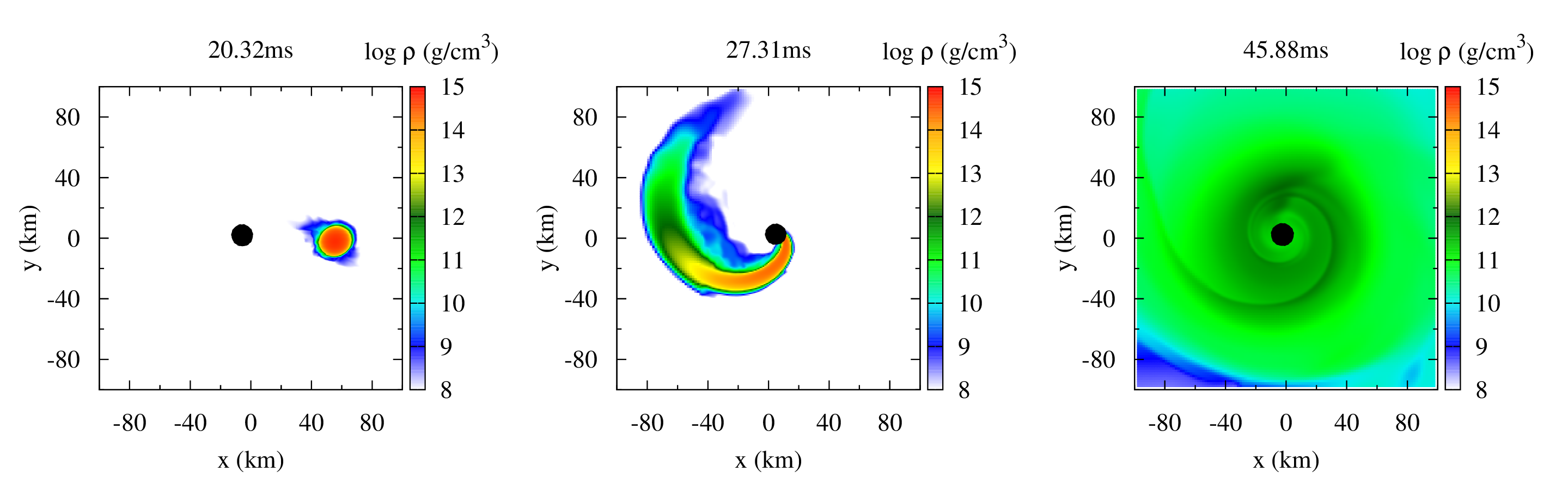
Figure 1: Rest-mass density profile on the equatorial plane in the central region at selected time slices for H4-Q5a75. Black filled circles show the interior of apparent horizons. The left, middle, and right panels correspond to a late inspiral phase, tidal tail formation, and quasistationary remnant accretion disk, respectively. The merger sets in at $t=$ $26.49\text{\,}\mathrm{ms}$ for this model.

We begin with a brief review of the dynamics of black hole-neutron star binary mergers (see Ref. Shibata and Taniguchi (2011) for details). Black hole-neutron star binaries evolve as a result of gravitational radiation reaction and eventually merge. Our initial conditions are chosen to evolve for $\sim$ 3.5 to 7.5 orbits before the merger, where the exact numbers depend on model parameters. Eccentricities are estimated to be $e\sim 0.01$–0.02 for all the models using methods described in Ref. Kyutoku et al. (2014), and they introduce uncertainties of the same order in the ejecta properties (see App. A.4 for the estimate).

The fate of the system after the merger is determined primarily by competition between the orbital separation at which tidal disruption occurs (hereafter, the tidal disruption radius), $r_{\mathrm{td}}$, and the radius of the innermost stable circular orbit, $r_{\mathrm{ISCO}}$. If $r_{\mathrm{ISCO}}$ is larger than $r_{\mathrm{td}}$, no appreciable tidal disruption occurs, and the neutron star is simply swallowed by the black hole. In this case, the remnant disk, fallback material, and ejecta are all negligible for our astrophysical interest. Although we do not pay particular attention to such cases in this study, models like APR4-Q3a0 and ALF2-Q7a5 fall into this category (see the next paragraph). By contrast, if $r_{\mathrm{td}}$ is larger than $r_{\mathrm{ISCO}}$, part of the disrupted material spreads around the black hole in the form of a tidal tail, while more than a half is still swallowed. Figure 1 shows rest-mass density profiles on the equatorial plane in the central region at selected time slices for H4-Q5a75 as an example of this category. Material that remains outside the apparent horizon can be divided into bound and unbound material, and the former always dominates the latter for the models considered in this study. The bound material may be further divided into disk and fallback components. The unbound component is generated primarily by tidal torque exerted on the elongated neutron star during tidal disruption, and details of the dynamical mass ejection process are described separately in Sec. III.2.

Appreciable tidal disruption occurs when (i) the neutron-star equation of state is stiff and the compactness is small, (ii) the mass ratio is small, and/or (iii) the black-hole spin is large (for a prograde orbit). These three conditions are reflected in our naming convention of the models. Note that, if we presume $M_{\mathrm{NS}}$ to be fixed, condition i can be rephrased as “the neutron-star radius is large” and condition ii as “the black-hole mass is small.” On one hand, $r_{\mathrm{td}}$ is expected to scale in the same way as the mass-shedding radius $r_{\mathrm{ms}}$, which is determined by the condition that the black-hole tidal force becomes equal to the neutron-star self-gravity at the stellar surface (see, e.g., Ref. Shibata and Taniguchi (2011)),

$$r_{\mathrm{td}}\propto r_{\mathrm{ms}}\sim Q^{1/3}R_{\mathrm{NS}},$$ (36)

and the dependence on the black-hole spin is not very strong Wiggins and Lai (2000); Ferrari et al. (2009). On the other hand, $r_{\mathrm{ISCO}}$ is written as $\hat{r}_{\mathrm{ISCO}}(\chi)M_{\mathrm{BH}}$, where $\hat{r}_{\mathrm{ISCO}}(\chi)$ is a decreasing function of the dimensionless spin parameter, $\chi$ Bardeen et al. (1972). Recalling $R_{\mathrm{NS}}/M_{\mathrm{BH}}=1/(\mathcal{C}Q)$, we expect the ratio to satisfy

$$\frac{r_{\mathrm{td}}}{r_{\mathrm{ISCO}}}\propto\frac{1}{\mathcal{C}Q^{2/3}\hat{r}_{\mathrm{ISCO}}(\chi)},$$ (37)

and a large value of this ratio should signal appreciable tidal disruption. This expectation has been verified by previous studies of disk formation and gravitational-wave emission Shibata and Taniguchi (2011), and Table 3 indicates that dynamical mass ejection also becomes efficient when these three parameters ($\mathcal{C}$, $Q$, and $\chi$) are advantageous for tidal disruption. The dependence of the ejecta properties on these parameters is discussed in more detail in Sec. III.3.

III.2 Mass ejection process and morphology

We first explain mechanisms of dynamical mass ejection and general properties of the ejecta by closely investigating APR4-Q3a75 in Sec. III.2.1. Mass ejection mechanisms and qualitative trends are the same for all the black hole-neutron star binary models simulated in this study, whereas differences in (semi)quantitative properties are found. We next discuss differences in the ejecta geometry among models in Sec. III.2.2. Characteristic quantities and their differences are described in Sec. III.3.

III.2.1 Case study: APR4-Q3a75

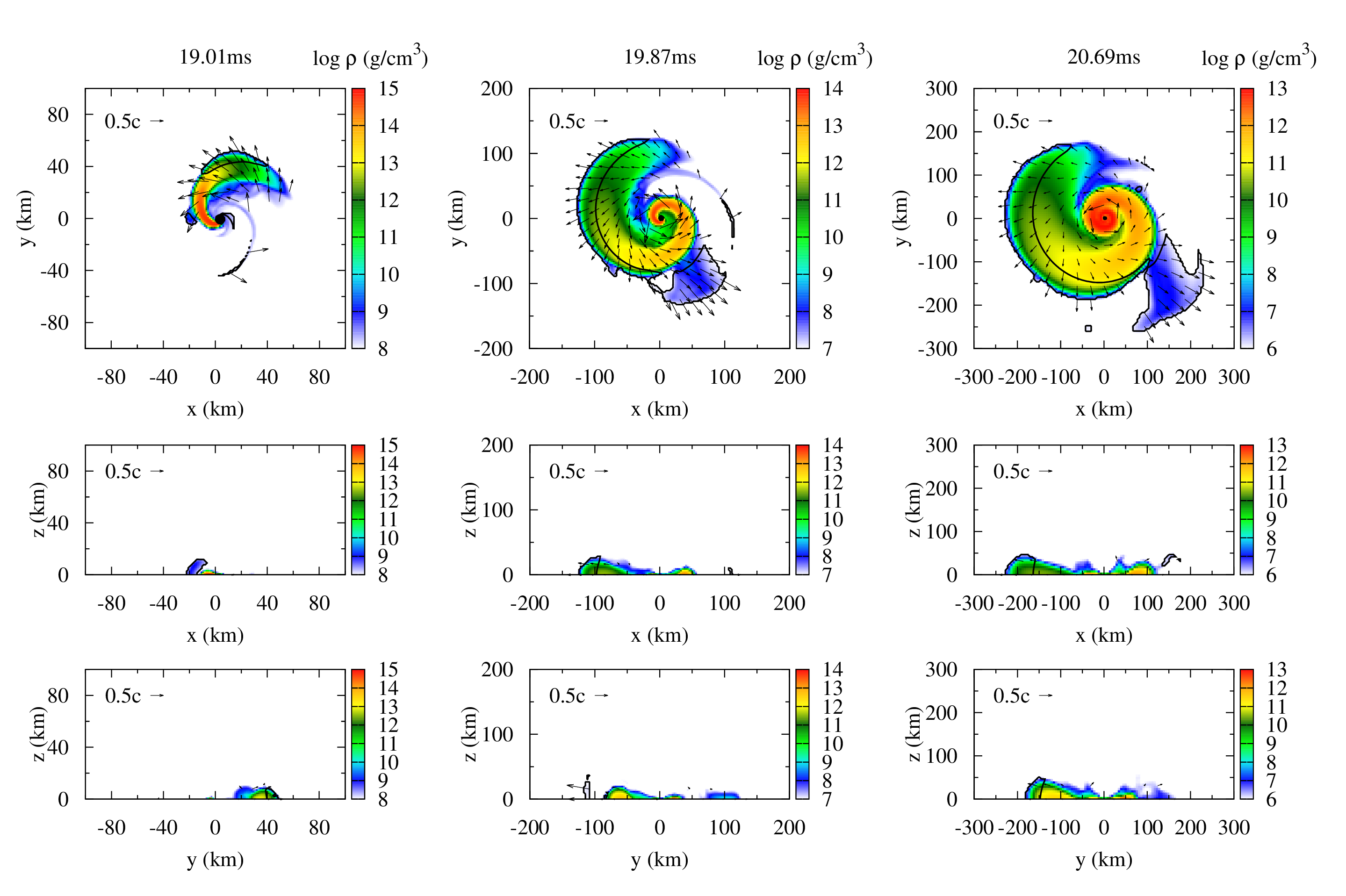
Figure 2: Rest-mass density profile for APR4-Q3a75 during the tidal disruption and dynamical mass ejection. Note the different spatial and density scales among the columns. Black filled circles show the interior of the apparent horizons. Black arrows show the spatial component of the covariant four-velocity, $u_{i}$. Unbound components satisfying $u_{t}<-1$ are marked by black curves, and we checked that contours marking $hu_{t}<-1$ nearly overlap with them. The top, middle, and bottom rows are the $xy$, $xz$, and $yz$ planes, respectively. The merger sets in at $t=$ $18.48\text{\,}\mathrm{ms}$ for this model. This figure should be compared with Figs. 3–5 of Ref. Hotokezaka et al. (2013a) where binary neutron stars are studied.

Figure 2 depicts the typical process of dynamical mass ejection at tidal disruption for model APR4-Q3a75. Once tidal disruption sets in, the neutron star is drastically elongated and forms a tidal tail. While the high-density innermost part is immediately swallowed by the black hole, the outer part spreads to a distant orbit and lags behind. Thus, the tidal tail exhibits a trailing one-armed spiral structure, and the black hole exerts tidal torque on the tail, increasing its orbital angular momentum. The outer part of the tail moves further outward due to the gain of the angular momentum, and the outermost part acquires enough kinetic energy to become unbound from the system, as marked by black curves in Fig. 2. In the course of this process, the pressure gradient in the tidal tail should also boost the outer part. This angular momentum transport proceeds in an unstable manner until the tidal tail winds around the black hole and collides with itself to form a nearly axisymmetric black hole-disk system. This mechanism generates most of the dynamical ejecta as well as bound material which eventually falls back to the black hole-disk system.

Although a small amount of unbound material appears to be ejected toward $\varphi\sim$$$ with a large velocity in Fig. 2, where $\varphi$ is the azimuthal angle in spherical coordinates, this appears to be an artifact created by the artificial atmosphere and finite grid resolutions as we discuss in Appendix A.5. This observation is consistent with Ref. Foucart et al. (2014). The mass, energy, and linear momentum of this component is negligible compared with the main component discussed in the previous paragraph, and thus the values shown in Table 3 are not affected.

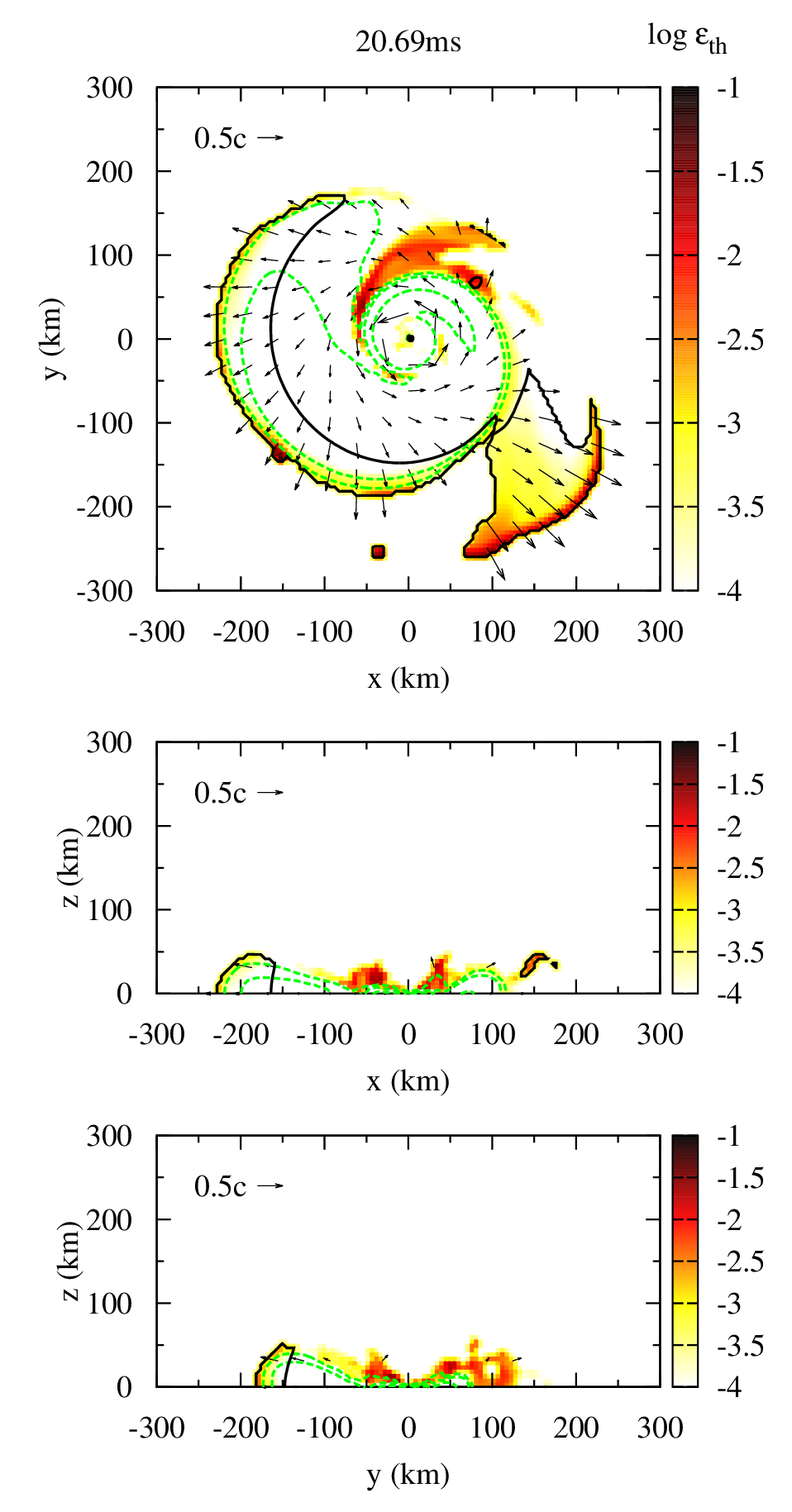
Figure 3: Profile of the thermal part of specific internal energy, $\varepsilon_{\mathrm{th}}$, for APR4-Q3a75. The time slice is taken to be the same as the right column of Fig. 2. The black filled circle, arrows, and curves have the same meanings as those in Fig. 2. Green dashed curves show contours of $\rho=${10}^{8}$$, ${10}^{10}$, and ${10}^{12}\text{\,}\mathrm{g}\text{\,}{\mathrm{cm}}^{-3}$. This figure should be compared with Figs. 7 and 8 of Ref. Hotokezaka et al. (2013a) where binary neutron stars are studied, taking different spatial scales into account.

Dynamical mass ejection from black hole-neutron star binaries is anisotropic Kyutoku et al. (2013). Figure 2 shows that the ejected material takes a crescentlike shape on the equatorial plane during its early evolution for APR4-Q3a75. Although the relative size of the central region occupied by bound material will become negligible as the rear velocity approaches zero (see below), the ejecta never sweep out the whole equatorial plane. Furthermore, it is concentrated around the equatorial plane and does not extend above the central black hole, because this mass ejection is driven by the tidal torque, which works most efficiently in the equatorial plane. This situation should be contrasted with dynamical mass ejection from binary neutron stars, in which quasiradial oscillations of remnant massive neutron stars eject an appreciable amount of material toward polar regions via shock interaction Hotokezaka et al. (2013a). To elucidate the difference, we show the thermal part of specific internal energy, $\varepsilon_{\mathrm{th}}$, in Fig. 3. As shocks do not play a role, the tidal tail including the ejecta is not heated significantly except for the self-colliding region of the tidal tail. The self-colliding shock interaction eventually thermalizes and circularizes material in the central region, and a hot accretion disk is formed. We will discuss properties of the accretion disk later (see also Sec. III.6). Apparent heating at the outermost part of the tidal tail is caused by the artificial atmosphere and is thus spurious.

Figures 2 and 3 suggest that the dynamical ejecta originates from the outer core and crust of the neutron star retaining its very low electron fraction (the number of electrons per baryon), $Y_{e}\lesssim 0.1$, at zero temperature Akmal et al. (1998). Because $M_{\mathrm{ej}}$ for APR4-Q3a75 is comparable to the typical mass of neutron-star crusts, $0.01M_{\odot}$ (see, e.g., Ref. Chamel and Haensel (2008)), the ejecta stripped from the outermost part of the tidal tail in a highly nonspherical manner stems not only from the crust but also from the core (see also Fig. 3 of Ref. Just et al. (2015)). In fact, $M_{\mathrm{ej}}$ for other binary models can easily exceed the typical crust mass. Nevertheless, the ejecta would not come from the inner core, because the densest part of the neutron star is swallowed by the black hole and bound material separates the black hole and ejecta. Thus, the dynamical ejecta should come mainly from the outer core and partly from the crust. The absence of shocks suggests that the low electron fraction of the outer core is not modified very much during dynamical mass ejection, and this is consistent with results obtained by previous smoothed-particle-hydrodynamics simulations Rosswog (2005); Rosswog et al. (2013); Just et al. (2015). Such ejecta are expected to be a promising site of r-process nucleosynthesis producing predominantly second- and third-peak elements via fission cycling, while the production of first-peak elements may not accompany Wanajo et al. (2014); Bauswein et al. (2014). It has to be cautioned that this estimation is speculative to some extent, because our simulations are performed without taking the electron fraction into account. We plan to revisit this topic with more sophisticated equations of state and neutrino transport schemes Sekiguchi et al. (2015).

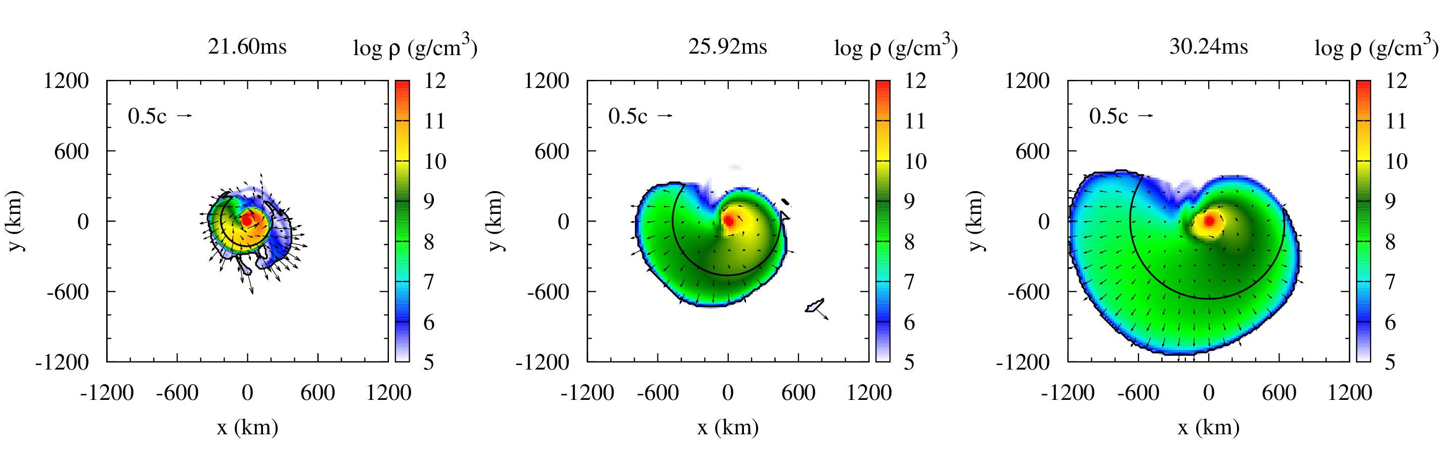
Figure 4: The same as Fig. 2, but on the equatorial plane at late times in the distant region. The black curves and arrows have the same meanings as those in Fig. 2. In this model, the ejecta linear momentum points toward $\Phi_{\mathrm{ej}}\approx$$$, i.e., close to the $-y$ direction [see Eq. (24) for the definition].

Figure 4 shows the long-term evolution of the dynamical ejecta in the distant region. This figure shows that the outer edge of the ejecta expands in a nearly homogeneous manner after the angular momentum transport by the tidal torque ceases. The azimuthal component of velocity decreases approximately as $r^{-1}$ due to angular momentum conservation and soon becomes negligible compared to the radial component as shown in Fig. 4. This implies that the kinetic energy of the ejecta is dominated by the radial velocity, and thus the average velocity, $v_{\mathrm{ave}}$, estimated from the kinetic energy approximately equals the typical radial velocity. Opening angles of ejecta in the equatorial and also meridional (not shown in Fig. 4) planes are approximately conserved, because the direction of velocity does not change appreciably once hydrodynamic interaction becomes negligible. Note that energy injection by the r-process heating will moderately change the ejecta geometry Rosswog et al. (2014).

Figure 4 also shows that the radial thickness of the dynamical ejecta increases in the long-term evolution of the ejecta, because the ejecta head is faster than the rear. Specifically, the head will maintain a velocity on the order of the escape velocity of the neutron star, while the rear velocity will approach zero (separation of bound and unbound components) as the material climbs up the gravitational potential well. The radius of the central bound region will become negligible compared to the radial thickness of the dynamical ejecta for exactly the same reason.

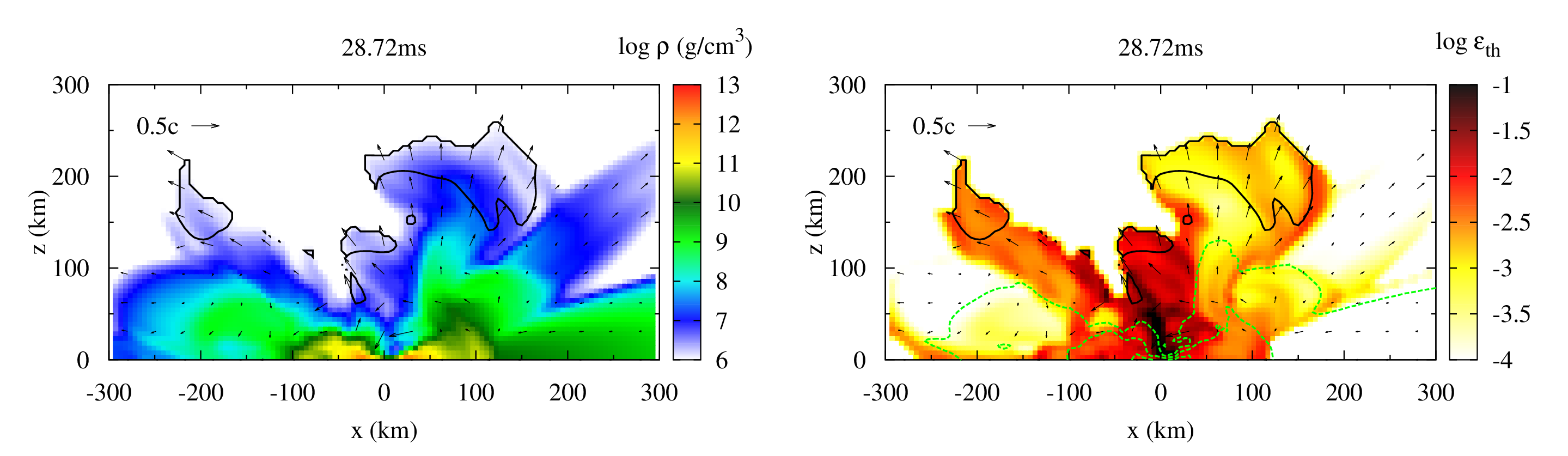
Figure 5: Profile of rest-mass density (left) and thermal part of the specific internal energy (right) on the $xz$ plane for APR4-Q3a75 after the disk formation. The black arrows and curves have the same meanings as those in Fig. 2. Green dashed curves show contours of $\rho=${10}^{8}$$, ${10}^{10}$, and ${10}^{12}\text{\,}\mathrm{g}\text{\,}{\mathrm{cm}}^{-3}$.

After disk formation, unbound material is newly generated from the disk region due to shock heating. Figure 5 shows the shock heating-driven disk outflow on the $xz$, meridional plane. When the tidal tail collides with itself, shock interaction increases $\varepsilon_{\mathrm{th}}$ near the contact surface. Because the rest-mass density is not high in the relevant region, thermal pressure dominates the cold-part pressure. The heated material expands, and some material is puffed up off the equatorial plane. In addition, shock interaction circularizes incoming tail material, and thus the disk region extends radially. Cold fallback material eventually accumulates and circulates around the outer edge of the hot disk material, as is visible from the right panel of Fig. 5 at $x\approx$120\text{\,}\mathrm{km}$$. When the accumulated cold material becomes very massive, shocks develop between the cold and hot material. Shock heating occurs continually at the outer edge of the disk due to this interaction, and material is also puffed up there. Material off the equatorial plane exhibits (seemingly) random motion, and a part of it collides with another part. Finally, some of the material is ejected from the system as hot blobs, and the rest eventually falls back to the disk surface. In contrast to dynamical mass ejection due to the tidal torque, this mechanism ejects material mainly toward nonequatorial (vertical) directions. As is evident from the left panel of Fig. 5, however, the mass of the ejecta generated by this heating is much smaller than that by the tidal torque. The situation will change if magnetic fields Kiuchi et al. , neutrino heating Just et al. (2015); Y. Sekiguchi et al. , and/or nuclear interactions Lee et al. (2009); Fernández and Metzger (2013) are taken into account, whereas a significant fraction of the disk material has to be ejected to dominate over dynamical mass ejection.

III.2.2 Variety of ejecta morphology

The ejecta geometry may be characterized by an opening angle in the equatorial plane, $\varphi_{\mathrm{ej}}$, and that in the meridional plane, $\theta_{\mathrm{ej}}$, where the latter is defined to refer only to material with $z\geq 0$, taking the equatorial symmetry into account. In the nearly spherical mass ejection expected for supernovae and binary neutron star mergers Hotokezaka et al. (2013a), $\varphi_{\mathrm{ej}}$ and $\theta_{\mathrm{ej}}$ should be regarded as $2\pi$ and $\pi/2$, respectively. We give estimates based on analytic arguments of the opening angles for black hole-neutron star binaries in Appendix B to compare with numerical results.

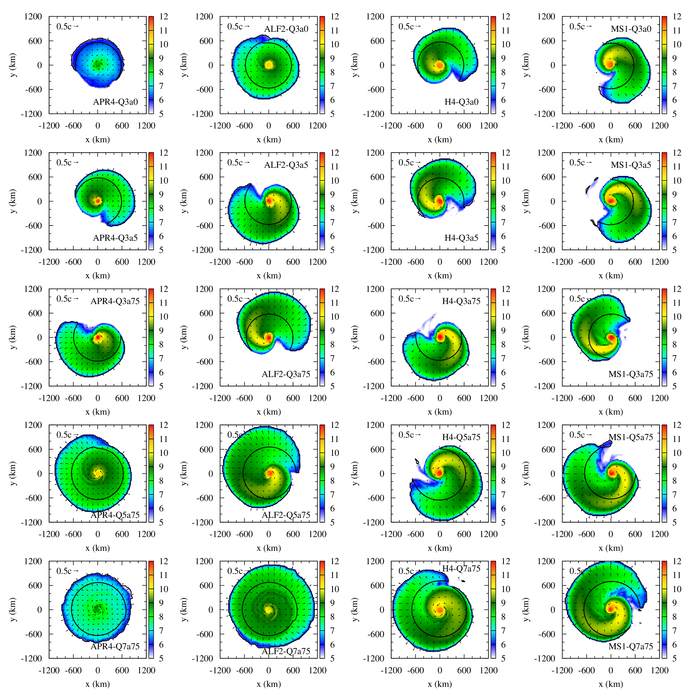
Figure 6: Rest-mass density profile on the equatorial plane for various models at $\approx$10\text{\,}\mathrm{ms}$$ after the onset of merger. Unbound components satisfying $u_{t}<-1$ are marked by black curves. From left to right, the equation of state is APR4, ALF2, H4, and MS1. From top to bottom, $(Q,\chi)$ is $(3,0)$, $(3,0.5)$, $(3,0.75)$, $(5,0.75)$, and $(7,0.75)$. The left panel on the third row is APR4-Q3a75 described in detail in Sec. III.2.1. Traces of rear-end collisions are found as bumps on inner black closed curves at $\varphi\approx\pi/2$ for ALF2-Q3a0 and APR4-Q5a75 and at $\varphi\approx 0$ for APR4Q7a75 and ALF2Q7a75.

Figure 6 shows the morphology of the dynamical ejecta on the equatorial plane for various models. This figure implies that a softer equation of state, a larger mass ratio, and a smaller black-hole spin lead to a larger value of $\varphi_{\mathrm{ej}}$ when other parameters are fixed. In particular for the case in which mass ejection is not very substantial, an unbound portion revolves more than one orbit ($\varphi_{\mathrm{ej}}>2\pi$) taking a spiral shape at generation, and rear-end collisions occur in overlapping directions to form a ring shape. Traces of the rear-end collisions are observed as bumps on boundaries between bound and unbound material (black closed curves) in Fig. 6. In these cases, the bulk velocity, $v_{\mathrm{ej}}$, is lower than $0.1c$ and is less than half of the average velocity, $v_{\mathrm{ave}}$ (see Table 3). The reason for this is that the ejecta linear momentum, $P_{\mathrm{ej}}$, is very small for nearly axisymmetric mass ejection.

This catalog suggests that $\varphi_{\mathrm{ej}}$ tends to become large when tidal disruption occurs only weakly. This tendency does not agree with the estimate obtained by time-scale arguments in Appendix B. A possible explanation of this tendency is the periastron advance in general relativity, which is pronounced when tidal disruption occurs very close to the innermost stable circular orbit Laguna et al. (1993). As an extreme example, orbital parameters of a test particle can be finely tuned so that it experiences an arbitrarily large number of revolutions traveling near marginally stable orbits Cutler et al. (1994); Glampedakis and Kennefick (2002). Although the ejecta material cannot be finely tuned due to its finite spatial extent and does not experience infinitely many revolutions, i.e., $\varphi_{\mathrm{ej}}$ will not diverge, the dynamical ejecta should be able to have a large value of $\varphi_{\mathrm{ej}}$ if the mass ejection takes place near the innermost stable circular orbit. Indeed, tidal disruption should have occurred very close to the innermost stable circular orbit, i.e., $r_{\mathrm{td}}\approx r_{\mathrm{ISCO}}$, when the ejecta mass is small but nonnegligible. This is consistent with the tendency observed in Fig. 6.

From the observational viewpoint, dynamical ejecta with a large opening angle, $\varphi_{\mathrm{ej}}\gtrsim 2\pi$, may not be very important, because a large opening angle is attained by the ejecta with a small mass, for which electromagnetic radiation is expected to be weak. Strong electromagnetic radiation should accompany substantial mass ejection, say $M_{\mathrm{ej}}\gtrsim 0.01M_{\odot}$, where $\varphi_{\mathrm{ej}}$ takes a value close to $\pi$ in most cases. However, substantial but nearly axisymmetric dynamical mass ejection such as that for ALF2-Q7a75 is not completely excluded.

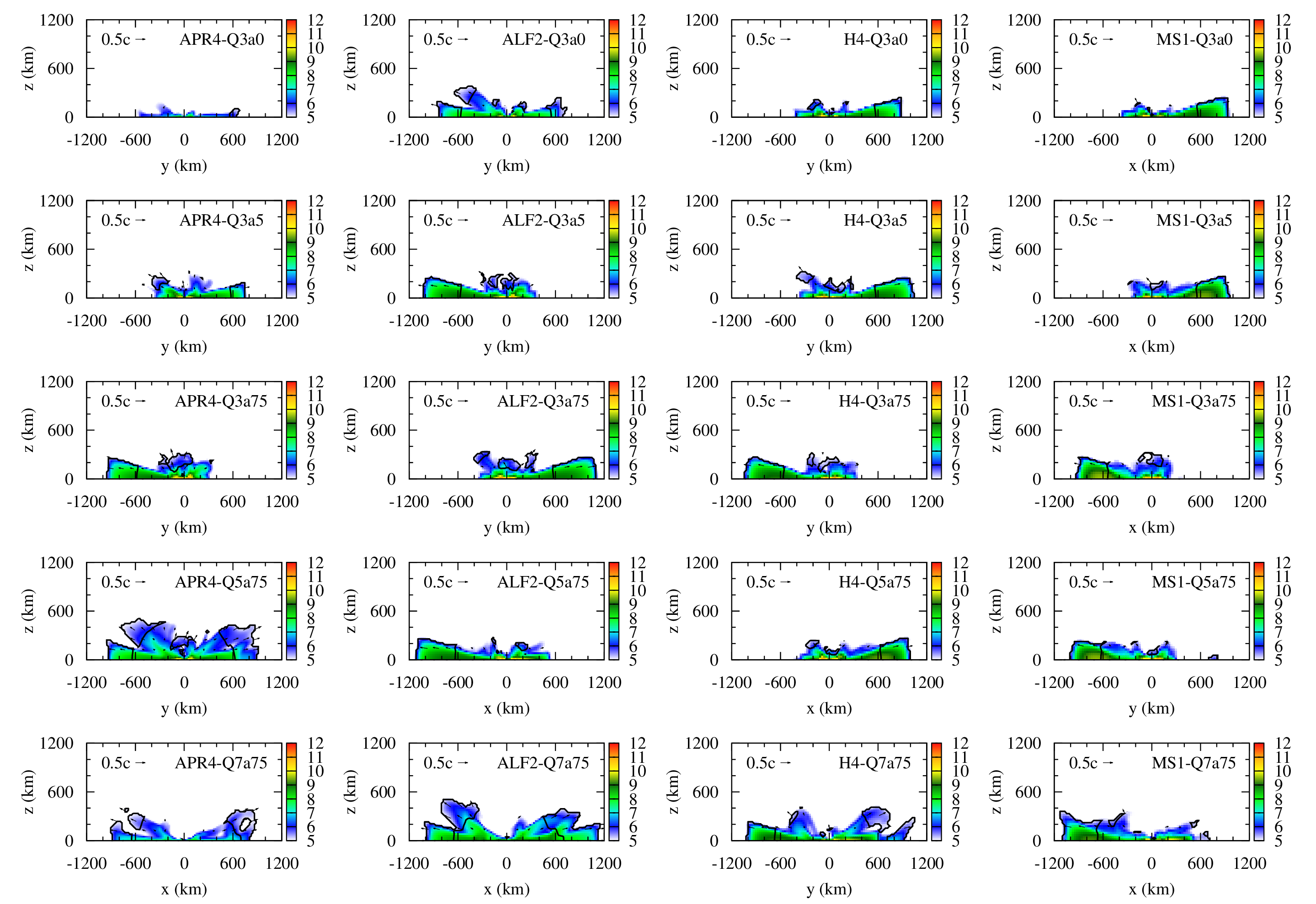
Figure 7: The same as Fig. 6 but on a meridional, $xz$ or $yz$ plane, chosen to be the one which is closer to the direction of $\Phi_{\mathrm{ej}}$. Unbound components satisfying $u_{t}<-1$ are marked by black curves. From left to right, the equation of state is APR4, ALF2, H4, and MS1. From top to bottom, $(Q,\chi)$ is $(3,0)$, $(3,0.5)$, $(3,0.75)$, $(5,0.75)$, and $(7,0.75)$. The left panel on the third row is APR4-Q3a75 described in detail in Sec. III.2.1.

The opening angle in the meridional plane does not differ very much among models as far as substantial mass ejection occurs. Figure 7 shows the morphology of the dynamical ejecta on the meridional plane for various models. This figure shows that the opening angle $\theta_{\mathrm{ej}}$ takes values between 1/5 and 1/3 (or $10\mathrm{°}$ and $20\mathrm{°}$) for cases with $M_{\mathrm{ej}}\gtrsim 0.01M_{\odot}$. The variation of $\theta_{\mathrm{ej}}$ up to a factor of $\lesssim 2$ is observed among models with substantial mass ejection, but the ejecta driven by the tidal torque never extend to, say, $\theta_{\mathrm{ej}}>$$$. At the same time, $\theta_{\mathrm{ej}}$ is very small when mass ejection is not efficient. Hence, sphericity is never achieved even approximately for cases considered in this study. This figure also suggests that $\theta_{\mathrm{ej}}$ tends to become small when $Q$ is large. This is consistent with the analytic expectation presented in Appendix B.

III.3 Characteristic quantities of ejecta

Here we discuss characteristic quantities of dynamical ejecta such as the mass and velocity, focusing on their dependence on binary parameters. As described in the beginning of this section, we measure ejecta quantities at $10\text{\,}\mathrm{ms}$ after the onset of merger. To check that estimation at that time gives acceptable results, we first investigate time evolution of the ejecta quantities in Sec. III.3.1. Next, we discuss the dependence in Sec. III.3.2.

III.3.1 Time evolution

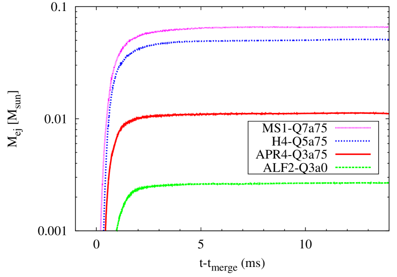
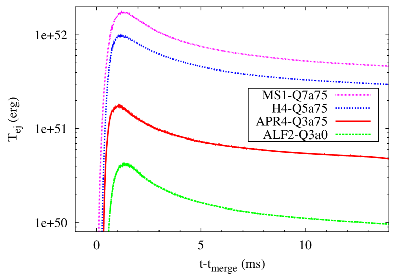
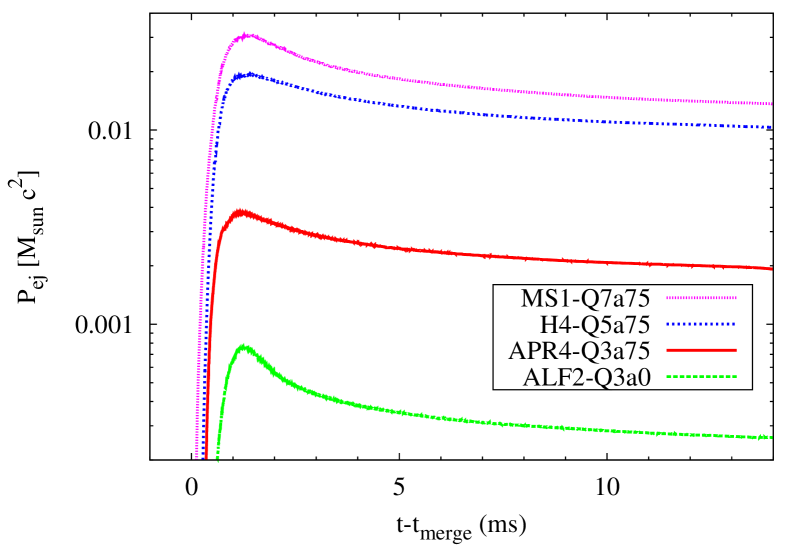
Figure 8: Time evolution of the mass (top), kinetic energy (middle), and linear momentum (bottom) of the ejecta for selected models.

Figure 8 shows the time evolution of $M_{\mathrm{ej}}$, $T_{\mathrm{ej}}$, and $P_{\mathrm{ej}}$ for selected models. All these values suddenly increase right after the onset of merger. The time evolution indicates that most of dynamical mass ejection progresses over $\approx$2\text{\,}\mathrm{ms}$$ and that the evolution relaxes afterward irrespective of the models.

The ejecta mass settles to a quasistationary value within $\sim$5\text{\,}\mathrm{ms}$$. This confirms the observation in Sec. III.2.1 that mass ejection due to disk activity does not contribute significantly to the total mass of the ejecta in our simulations. Therefore, the measurement of $M_{\mathrm{ej}}$ at $10\text{\,}\mathrm{ms}$ after the onset of merger is safely justified.

The kinetic energy and linear momentum peak at 1–$2\text{\,}\mathrm{ms}$ after the onset of merger and decrease afterward. The reason of this decrease is that the ejecta lose energy in climbing up the gravitational potential well of the central black hole-disk system. The Newtonian formulas indicate that $T_{\mathrm{ej}}$ measured at $10\text{\,}\mathrm{ms}$ after the onset of merger overestimates its final value by $(m_{0}M_{\mathrm{ej}}/r)/T_{\mathrm{ej}}\sim 30\%$–40% for models shown in Fig. 8, and this is consistent with the later evolution. This will result in $\sim 15\%$–20% overestimation of the ejecta velocity, and thus this error has to be kept in mind in the following discussions, along with those described in Appendix A. If we measure these values at $\lesssim$ $5\text{\,}\mathrm{ms}$ after the onset of merger and use them as proxies for their final values, final ejecta velocities can be overestimated nearly by 100%. Hence, a large computational domain is a prerequisite for an accurate study of mass ejection.

III.3.2 Dependence on binary parameters

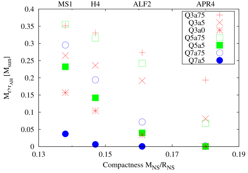
Figure 9: Mass remaining outside the apparent horizon composed of bound and unbound material, $M_{r>r_{\mathrm{AH}}}=M_{\mathrm{bd}}+M_{\mathrm{ej}}$, as functions of the compactness, $\mathcal{C}$.

We start by looking at the total mass remaining outside the apparent horizon, $M_{r>r_{\mathrm{AH}}}=M_{\mathrm{bd}}+M_{\mathrm{ej}}$, to check consistency with previous work. Figure 9 plots $M_{r>r_{\mathrm{AH}}}$ measured at $10\text{\,}\mathrm{ms}$ after the onset of merger (presented in Table 3) as a function of the compactness, $\mathcal{C}$. This figure supports the discussion in Sec. III.1. That is, a small neutron-star compactness, small mass ratio, and large black-hole spin increase the strength of the tidal disruption resulting in the increase of $M_{r>r_{\mathrm{AH}}}$. Our present simulations reproduce quantitatively the results of our previous simulations Kyutoku et al. (2010, 2011b, 2011a), as well as those by other authors (see Ref. Foucart (2012) for a compilation). The dependence of $M_{r>r_{\mathrm{AH}}}$ on $\mathcal{C}$ is approximately linear within the range studied here, until it levels off at $\lesssim 0.01M_{\odot}$. This suggests that the effect of neutron-star properties on $M_{r>r_{\mathrm{AH}}}$ is reasonably captured by the compactness, $\mathcal{C}$.

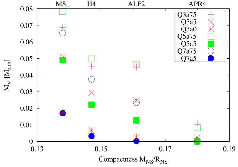
Figure 10: Ejecta mass, $M_{\mathrm{ej}}$, as a function of the compactness, $\mathcal{C}$.

The ejecta mass, $M_{\mathrm{ej}}$, is correlated with the strength of the tidal disruption as $M_{r>r_{\mathrm{AH}}}$ is, but the dependence of $M_{\mathrm{ej}}$ on binary parameters is complicated. Figure 10 shows $M_{\mathrm{ej}}$ as a function of $\mathcal{C}$. Plots of $T_{\mathrm{ej}}$ and $P_{\mathrm{ej}}$ exhibit similar behavior. For fixed values of $Q$ and $\chi$, $M_{\mathrm{ej}}$ increases as $\mathcal{C}$ decreases. This is qualitatively the same as $M_{r>r_{\mathrm{AH}}}$ and supports the expectation that strong tidal disruption is accompanied by efficient mass ejection. However, the correlation is weaker between $M_{\mathrm{ej}}$ and $\mathcal{C}$ than between $M_{r>r_{\mathrm{AH}}}$ and $\mathcal{C}$ for fixed values of $Q$ and $\chi$. This suggests that the boundary separating bound and unbound material, $u_{t}=-1$, is not determined solely by the compactness but is also sensitive to the stellar structure. This observation is consistent with Ref. Foucart et al. (2014), which found a similar fact by comparing their results with some of our results reported in Ref. Hotokezaka et al. (2013b). It is reasonable that detailed properties of the equation of state could play an important role during dynamical mass ejection via effects such as the pressure gradient and/or central condensation.

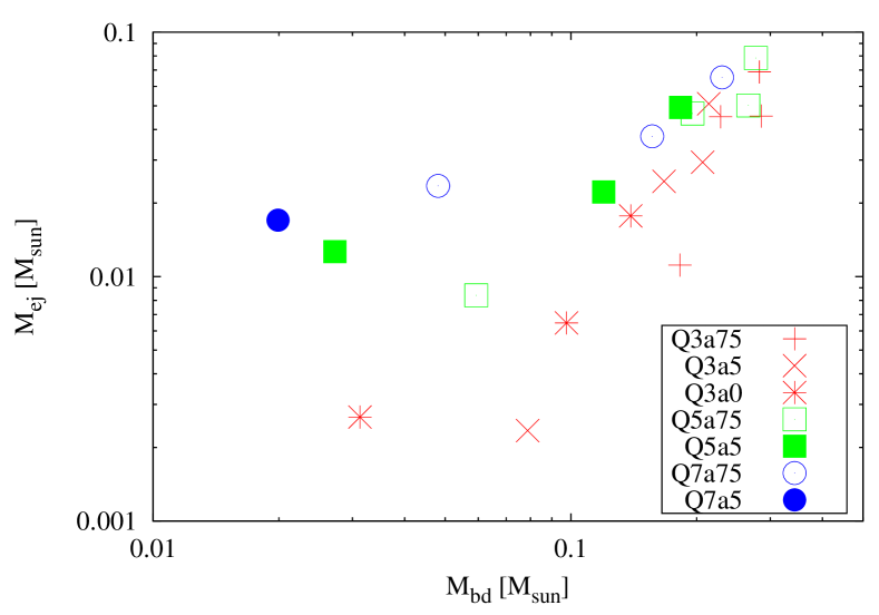
Figure 11: Correlation between the ejecta mass, $M_{\mathrm{ej}}$, and bound mass, $M_{\mathrm{bd}}$. We restrict the region to $M_{\mathrm{ej}}\geq 0.001M_{\odot}$ and $M_{\mathrm{bd}}\geq 0.01M_{\odot}$, where the results are astrophysically interesting.

The ejecta mass, $M_{\mathrm{ej}}$, does not depend monotonically on the mass ratio, $Q$, for fixed values of $\mathcal{C}$ and $\chi$ (see Fig. 10). The reason for this is that the ejecta tends to comprise a large fraction of material remaining outside the apparent horizon for a large mass ratio, especially when tidal disruption is weak and $M_{r>r_{\mathrm{AH}}}$ is not very large. Figure 11 shows the correlation between the ejecta mass, $M_{\mathrm{ej}}$, and bound mass, $M_{\mathrm{bd}}$. This figure indicates that $M_{\mathrm{ej}}$ does not decrease very rapidly with the decrease of $M_{\mathrm{bd}}$ (and equivalently $M_{r>r_{\mathrm{AH}}}$) for a large value of $Q$. Specifically, $M_{\mathrm{ej}}\geq 0.01M_{\odot}$ can be achieved when $M_{\mathrm{bd}}\gtrsim 0.01M_{\odot}$ for $Q=7$, while it is possible only when $M_{\mathrm{bd}}\gtrsim 0.1M_{\odot}$ for $Q=3$. The fact that mass ejection can be substantial even if tidal disruption is not very strong for a large value of $Q$ is encouraging for electromagnetic counterpart searches, because astrophysical black holes are expected to prefer large mass ratios Özel et al. (2010); Kreidberg et al. (2012).

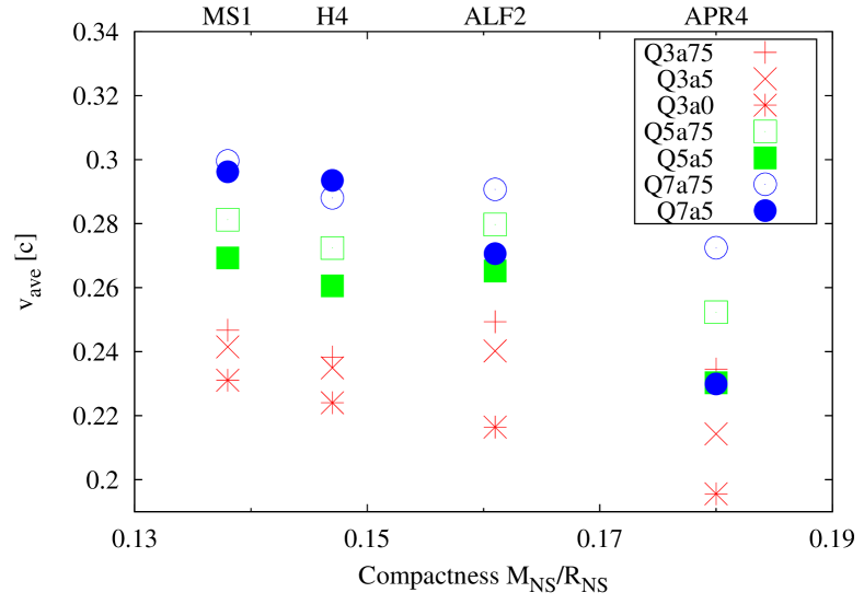
Figure 12: Average velocity of the ejecta, $v_{\mathrm{ave}}$, defined from the kinetic energy, $T_{\mathrm{ej}}$, as a function of the compactness, $\mathcal{C}$.

The increase of $M_{\mathrm{ej}}/M_{\mathrm{bd}}$ with the mass ratio, $Q$, implies that material remaining outside the apparent horizon tends to become more energetic when $Q$ is larger. This speculation is supported by the fact that the average velocity of the ejecta, $v_{\mathrm{ave}}$, is larger for a larger mass ratio. Figure 12 shows $v_{\mathrm{ave}}$ as a function of $\mathcal{C}$. A typical value of $v_{\mathrm{ave}}$ is 0.22–$0.25c$ for $Q=3$, and this rises to 0.25–$0.28c$ for $Q=5$ and 0.28–$0.3c$ for $Q=7$. This can be ascribed to the higher energy of material remaining outside the apparent horizon for a larger value of $Q$. The effect of the mass ratio on ejecta velocities via a gravitational potential is pointed out in the context of the tidal disruption of a main sequence star during a nearly parabolic encounter with a supermassive black hole, where a half of the star is expected to become unbound Lacy et al. (1982). Although the qualitative trend is the same, dynamical processes should play a crucial role in realizing this dependence in the inspiral of black hole-neutron star binaries, because all the neutron-star material is bound to the system at the onset of tidal disruption. Note that the systematic error in $v_{\mathrm{ave}}$ associated with the residual gravitational binding described in Sec. III.3.1 is not likely to modify this tendency qualitatively, because all the values of $v_{\mathrm{ave}}$ are systematically overestimated.

The dependence of the ejecta mass, $M_{\mathrm{ej}}$, on the black-hole spin, $\chi$, is simpler than that on $\mathcal{C}$ and $Q$ (see Fig. 10). Namely, a large black-hole spin increases the amount of ejecta for fixed values of $\mathcal{C}$ and $Q$. We do not find significant dependence of $M_{\mathrm{ej}}/M_{\mathrm{bd}}$ on $\chi$. The average velocity, $v_{\mathrm{ave}}$, tends to increase as $\chi$ increases.

The ejecta mass, $M_{\mathrm{ej}}$, is correlated with the mass remaining outside the apparent horizon, $M_{r>r_{\mathrm{AH}}}$, as indicated in Fig. 11. Quantitatively, we obtain

$$\frac{M_{\mathrm{ej}}}{M_{\odot}}=(0.27\pm 0.07)\left(\frac{M_{r>r_{\mathrm{AH}}}}{M_{\odot}}\right)^{1.3\pm 0.2},$$ (38)

by fitting all the data shown in Table 3 with equal weights, where the range indicates the 1-$\sigma$ asymptotic standard error. If we fit the data of models with different values of $Q$ separately, relations become

$$\frac{M_{\mathrm{ej}}}{M_{\odot}}=\begin{cases}(0.41\pm 0.14)\left(M_{r>r_{\mathrm{AH}}}/M_{\odot}\right)^{1.8\pm 0.3}&(Q=3)\\ (0.23\pm 0.06)\left(M_{r>r_{\mathrm{AH}}}/M_{\odot}\right)^{1.1\pm 0.2}&(Q=5)\\ (0.15\pm 0.02)\left(M_{r>r_{\mathrm{AH}}}/M_{\odot}\right)^{0.73\pm 0.09}&(Q=7)\end{cases}.$$ (39)

It is evident that the power-law index is smaller for a larger value of $Q$, and thus the separate fitting may be more appropriate. These relations give us an approximate estimate of $M_{\mathrm{ej}}$ combined with a fitting formula for $M_{r>r_{\mathrm{AH}}}$ provided in Ref. Foucart (2012). Sources of the error come from both simulations and fitting procedures, and only the latter is taken into account in Eqs. (38) and (39).

III.4 Ejecta and envelope structure

First in Sec. III.4.1, we investigate matter profiles on the equatorial plane, where most of the material resides. It includes disk, fallback, and ejecta components. Next, material distribution along the $z$ axis is investigated in Sec. III.4.2. It will be important for gamma-ray bursts, because a hypothetical jet (or fireball) can achieve an ultrarelativistic velocity only if the baryon load is not very high Mészáros and Rees (2000). Finally, we investigate the velocity distribution of dynamical ejecta in Sec. III.4.3, which is required to predict electromagnetic radiation quantitatively Piran et al. (2013); Kisaka et al. (2015). Detailed structures of material obtained from our simulations are not expected to be very realistic, because the equation of state in a relevant regime is composed of a single zero-temperature polytrope and ideal-gas-like thermal correction. We still believe that our results capture qualitative properties of the material structure, particularly for ejecta in distant regions where hydrodynamic interaction does not play an important role.

III.4.1 Equatorial plane

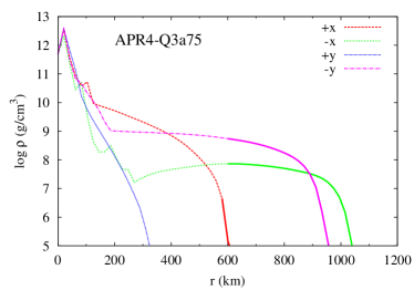
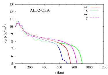
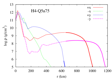
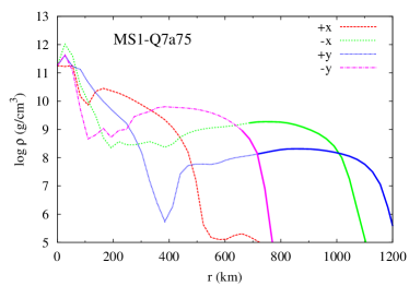
Figure 13: Rest-mass density in the logarithmic scale along the $x$ and $y$ axes at $10\text{\,}\mathrm{ms}$ after the onset of merger for the selected models. Positive and negative directions are plotted separately. Solid and dashed portions of each curve denote unbound and bound material, respectively. Corresponding plots in Fig. 6 are the third row and first column for the top left (APR4-Q3a75), first row and second column for the top right (ALF2-Q3a0), fourth row and third column for the bottom left (H4-Q5a75), and fifth row and fourth column for the bottom right (MS1-Q7a75).

Figure 13 shows density profiles along the $x$ and $y$ axes at $10\text{\,}\mathrm{ms}$ after the onset of merger for selected models. Corresponding snapshots are given in Fig. 6. The material at $r\lesssim$ $100\text{\,}\mathrm{km}$ is in an approximately axisymmetric state for all the models. This implies that accretion disks are formed in the central regions at this time. For a given value of $M_{r>r_{\mathrm{AH}}}$, the rest-mass density in the disk region is higher when $Q$ is smaller. The reason for this is that characteristic length scales are proportional to the total mass of the system, and thus to $Q+1$. Accordingly, characteristic rest-mass density should be proportional to $(Q+1)^{-2}$ for a given value of $M_{r>r_{\mathrm{AH}}}$. This tendency was already reported in Ref. Kyutoku et al. (2011a).

Density profiles outside the disk region depend significantly on the azimuthal angle. On one hand, the rest-mass density steeply decreases along directions with no ejecta. In Fig. 13, the $+y$ direction of APR4-Q3a75 and $-x$ direction of H4-Q5a75 fall into this category. The $+x$ direction of MS1-Q7a75 also corresponds to this case, but a high-density region is still observed up to $\approx$500\text{\,}\mathrm{km}$$, because the tidal tail has not fallen back and collided with itself yet in this direction. On the other hand, approximately constant density plateaus extend up to $\sim$1000\text{\,}\mathrm{km}$$ along directions that the ejecta sweep. For example, the $-x$ and $-y$ directions of APR4-Q3a75 exhibit sudden changes of the structure at $\approx$200\text{\,}\mathrm{km}$$ from a steep decline to plateaus. Similar situations are also found in the $+x$ and $-y$ directions of H4-Q5a75 and $-x$ and $+y$ directions of MS1-Q7a75, except for pronounced low-density regions between disk regions and plateaus. These gaps are more prominent for systems with a larger neutron-star radius at a fixed time (i.e., $10\text{\,}\mathrm{ms}$) from the onset of merger and eventually disappear as tidal tails fall back. When material spreads in a nearly axisymmetric manner with $\varphi_{\mathrm{ej}}\gtrsim 2\pi$, plateaulike profiles are observed in all the directions like ALF2-Q3a0. In any case, the plateaus change to rapidly decaying profiles at their outer edges.

The ejecta as an unbound portion is smoothly connected to a bound portion in the plateau regions. When the ejecta mass is large, the ejecta tends to occupy a large fraction of plateau material, particularly along a direction with the fastest expansion. The highest-density direction always disagrees with the fastest-expanding direction, in which the rest-mass density is typically lower by an order of magnitude at a given radius than the highest. For example, the rest-mass density of the ejecta is the highest in the $-y$ direction for APR4-Q3a75, whereas the fastest direction is the $-x$ direction. This is because low-density material is ejected from the outer part of neutron stars prior to the high-density material from the inner part during mass ejection driven by the tidal torque. The ejecta of ALF2-Q3a0 is more axisymmetric than those of the other models, and a bump at $\approx$650\text{\,}\mathrm{km}$$ in the $+y$ direction reflects the rear-end collision of the tidal tail with $\varphi_{\mathrm{ej}}>2\pi$. Note that the spatial distribution of the dynamical ejecta is different from that for binary neutron star mergers, where a moderately steep power law with the index $\approx-3.5$ is observed Nagakura et al. (2014).

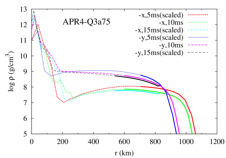
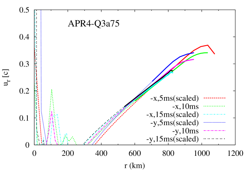
Figure 14: Rest-mass density on a logarithmic scale (top) and radial velocity (bottom) along the $-x$ and $-y$ directions at 5, 10, and $15\text{\,}\mathrm{ms}$ after the onset of merger for APR4-Q3a75. Solid and dashed portions of each curve denote unbound and bound material, respectively. Assuming homologous expansion, the radius is multiplied by 2 for the $5\text{\,}\mathrm{ms}$ profile and divided by 1.5 for the $15\text{\,}\mathrm{ms}$ profile, so that they can be compared directly with that at $10\text{\,}\mathrm{ms}$. Similarly, the density is divided by $2^{3}$ for the $5\text{\,}\mathrm{ms}$ profile and multiplied by $(1.5)^{3}$ for the $15\text{\,}\mathrm{ms}$ profile. The velocity is not scaled and is truncated at $\rho=${10}^{5}\text{\,}\mathrm{g}\text{\,}{\mathrm{cm}}^{-3}$$ to avoid showing artificial atmospheres accumulated near ejecta surfaces. Truncation of profiles at $\approx$850\text{\,}\mathrm{km}$$ for $15\text{\,}\mathrm{ms}$ is due to escape of material from the second largest domain, outside which hydrodynamic evolution equations are not solved.

The ejecta evolves in an approximately homologous manner. That is, the velocity of each fluid element is kept approximately constant, and its position and density evolve according to the free-expansion law,

$$r\propto t\;,\;\rho\propto t^{-3}.$$ (40)

Figure 14 shows rest-mass density and velocity profiles at 5, 10, and $15\text{\,}\mathrm{ms}$ after the onset of merger in the $-x$ and $-y$ directions of APR4-Q3a75. In these plots, the radius and rest-mass density are scaled according to Eq. (40) so that those at 5 and $15\text{\,}\mathrm{ms}$ can be compared directly to those at $10\text{\,}\mathrm{ms}$. Both the density and velocity profiles overlap approximately among different time slices after the scaling, and the agreement is particularly good between 10 and $15\text{\,}\mathrm{ms}$. These facts imply that homologous expansion is achieved at the late phase. We also observe approximate homologous expansion for other models, but the deviation is slightly more severe for a larger value of $Q$ at a fixed time (i.e., $10\text{\,}\mathrm{ms}$) due probably to stronger residual gravitational binding.

III.4.2 Polar direction

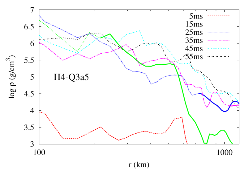
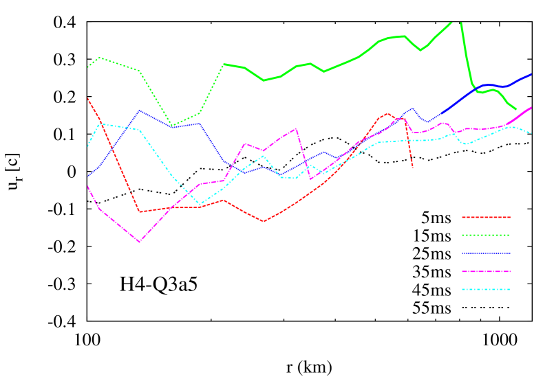
Figure 15: Rest-mass density in the logarithmic scale (top) and radial velocity (bottom) along the $z$ axis at several time slices for H4-Q3a5. Distances are also shown in the logarithmic scale. The time is given as that after the onset of merger, $t_{\mathrm{merge}}$. Solid and dashed portions of each curve denote unbound and bound material, respectively. The velocity of material with $\rho\leq${10}^{3}\text{\,}\mathrm{g}\text{\,}{\mathrm{cm}}^{-1}\text{\,}{\mathrm{}}^{3}$$ is not shown.

Figure 15 shows rest-mass density and velocity profiles along the $z$ axis for H4-Q3a5. Because our purpose is to study the formation of an envelope, profiles at several time slices are shown together without scalings. At $5\text{\,}\mathrm{ms}$ after the onset of merger, no unbound material is found, and the rest-mass density is very low everywhere. This is because the tidal torque does not eject material toward the polar region. Material is pushed significantly toward the polar region only after the shock heating in the disk region sets in. This is reflected in the increase of the rest-mass density for $t-t_{\mathrm{merge}}\gtrsim$10\text{\,}\mathrm{ms}$$. Unbound material is ejected from the disk with $v\approx 0.3c$ in the beginning and is beyond a radius of $1000\text{\,}\mathrm{km}$ by $\approx$35\text{\,}\mathrm{ms}$$ for this particular model.

A long-lived envelope is formed following the shock-driven disk outflow. The velocity of envelope material is smaller than the typical ejecta velocity, and in particular, the radial velocity of bound material falls below $0.1c$ at $55\text{\,}\mathrm{ms}$. This suggests that the envelope is in an approximately stationary state at this time. Indeed, the rest-mass density profiles do not change very much from 25 to $55\text{\,}\mathrm{ms}$. The profile may be approximated by a power law, $\rho\propto r^{-p_{\mathrm{env}}}$, with its index $p_{\mathrm{env}}\approx 2$–3. The magnitude of the rest-mass density implies that the total mass of the envelope formed after the merger of H4-Q3a5 is much smaller than that formed after binary neutron star mergers Hotokezaka et al. (2013a); Nagakura et al. (2014). This could be advantageous for a hypothetical jet to overcome a baryon loading problem, but it will not be easy to obtain a collimated jet in the absence of a heavy envelope. Firm conclusions to the jet propagation require an extensive study of disk winds.

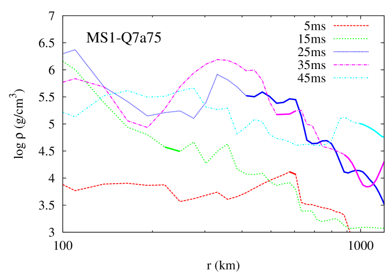
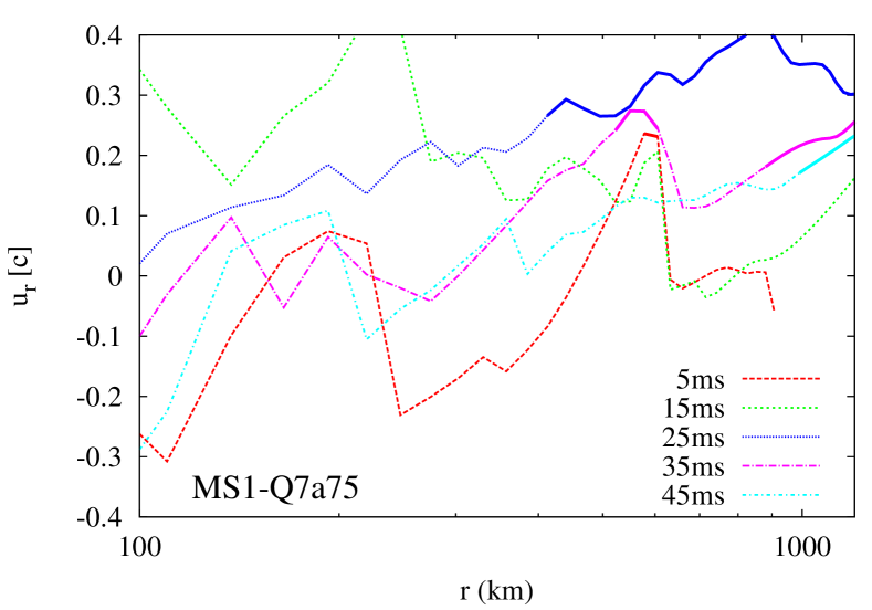
Figure 16: The same as Fig. 15 but for MS1-Q7a75.

It takes a long time for the remnant of a high-mass-ratio binary merger to develop a long-lived envelope in the polar region. Figure 16 shows rest-mass density and velocity profiles along the $z$ axis for MS1-Q7a75. In this model, the ejecta generated by the disk are beyond $1000\text{\,}\mathrm{km}$ only for $t-t_{\mathrm{merge}}\gtrsim$45\text{\,}\mathrm{ms}$$, and material behind it exhibits significantly more time variability than that of H4-Q3a5. The velocity profile with $v\gtrsim 0.1c$ also indicates significant time variability. It can, however, still be seen that the rest-mass density of the envelope is comparable to that of H4-Q3a5 (Fig. 15). Thus, we may safely conclude that the mass of the envelope formed after the merger is much smaller for black hole-neutron star binaries than for binary neutron stars unless (or possibly even if) binary parameters are extreme as far as the dynamical processes are concerned.

III.4.3 Velocity distribution

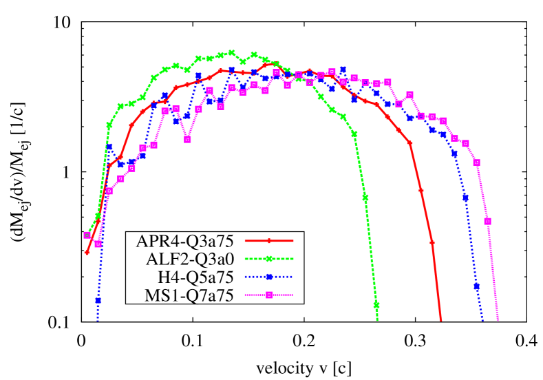
Figure 17: Velocity distribution normalized by the ejecta mass measured at $10\text{\,}\mathrm{ms}$ after the onset of merger for selected models. The velocity is defined as $\sqrt{1-1/(-u_{t})^{2}}$. We use $dM_{\mathrm{ej}}/dv$ rather than its integration over a finite velocity interval, because the former quantity is independent of binning.

Figure 17 shows the velocity distributions of dynamical ejecta normalized by the ejecta mass, $M_{\mathrm{ej}}$, measured at $10\text{\,}\mathrm{ms}$ after the onset of merger for selected models. Namely, integrating each distribution over the velocity returns unity. They are derived by analyzing unbound material on the equatorial plane as described in Sec. II.5.1, and we checked that estimation at different time slices gives very similar results.

All the models exhibit a relatively flat distribution with a cutoff at low and high velocities rather than, say, a power-law distribution. This agrees semiquantitatively with previous results obtained in Newtonian simulations Rosswog et al. (2013). This distribution implies that the density structure of ejecta can be approximated by $\rho\propto v^{-2}\propto r^{-2}$ within the range between lower and higher cutoff velocities, because the free-expansion law, Eq. (40), gives $dM/dv\propto\rho v^{2}$. This observation is largely consistent with the spatial profile shown in Fig. 13.

The velocity distribution is shifted toward larger velocities when the ejecta mass is larger (see the top panel of Fig. 8 for visual comparisons). We also find that the distribution tends to be shifted toward larger velocities when the mass ratio, $Q$, is larger. This is consistent with the observations of $M_{\mathrm{ej}}/M_{\mathrm{bd}}$ and $v_{\mathrm{ave}}$ in Sec. III.3.2, where the dynamical ejecta from a higher-mass-ratio binary is seen to be energetic. Previous numerical-relativity simulations also found this tendency Foucart et al. (2014).

III.5 Fallback

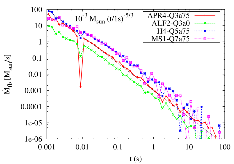
Figure 18: Fallback rate measured by analyzing matter profiles at $10\text{\,}\mathrm{ms}$ after the onset of merger for selected models. A power law $${10}^{-3}$M_{\odot}~{}${\mathrm{s}}^{-1}$(t/$1\text{\,}\mathrm{s}$)^{-5/3}$ is also plotted (black dot-dashed line) as an eye guide. Apparent deviation from the power law at $t\gtrsim$ $1\text{\,}\mathrm{s}$ is ascribed to the limited number of grid data, and the power law is recovered if we compute $\dot{M}_{\mathrm{fb}}$ using a wide time interval.

The fallback rate as a function of time is found to obey a power law with the index $-5/3$ irrespective of the models. Figure 18 shows fallback rates determined by the method described in Sec. II.5.2 analyzing matter profiles at $10\text{\,}\mathrm{ms}$ after the onset of merger for the selected models. Aside from statistical fluctuations due to the limited number of grid data, overall behavior is consistent with the structureless power law, $\dot{M}_{\mathrm{fb}}\propto t^{-5/3}$, and no significant time evolution is found when we compute $\dot{M}_{\mathrm{fb}}$ at different time slices. This power-law fallback rate is known to be achieved after the tidal disruption of main sequence stars by supermassive black holes Rees (1988); Phinney (1989). The same power law is found for black hole-neutron star binaries in Newtonian simulations Rosswog (2007); Rosswog et al. (2013) and is also reported in a numerical-relativity simulation for a single binary model with the $\Gamma=2$ polytrope Chawla et al. (2010). Our results confirm their findings for a wide range of binary parameters in numerical relativity. Nuclear interaction neglected in this study may not be important, because Newtonian studies show that nucleosynthesis in the nuclear statistical equilibrium does not modify the power-law behavior Rosswog (2007); Rosswog et al. (2013) and r-process heating can modify it only on rare occasions Metzger et al. (2010b).

This power-law behavior implies that the mass spectrum with respect to specific energy takes a constant profile, i.e., $dM_{\mathrm{fb}}/d\tilde{E}=\mathrm{const}$. The usual reasoning behind the power-law index $-5/3$ is the combination of $dM_{\mathrm{fb}}/dP_{\mathrm{fb}}=(dM_{\mathrm{fb}}/d\tilde{E})(d\tilde{E}/dP_{\mathrm{fb}})$, the Keplerian relation $P_{\mathrm{fb}}\propto a_{\mathrm{fb}}^{3/2}\propto(-\tilde{E})^{-3/2}$, and the assumption that $dM_{\mathrm{fb}}/d\tilde{E}$ is constant. The first and second relations are universal. The third assumption is verified for the tidal disruption of main sequence stars by various hydrodynamic simulations (e.g., Ref. Evans and Kochanek (1989)) and is pointed out to be more appropriate for a stiffer polytrope due to stronger shock interaction Lodato et al. (2009). Because the neutron-star self-gravity cannot be neglected and shocks do not appear to play a significant role in energy redistribution for a neutron star disrupted by a stellar-mass black hole, the reason for constant energy distribution is nontrivial and may be worth future investigation.

Although the overall magnitude of the power law is not computed very accurately by our approximate estimation method, we may safely conclude that the fallback rates span $\dot{M}_{\mathrm{fb}}\sim${10}^{-4}$$–$${10}^{-2}$M_{\odot}~{}${\mathrm{s}}^{-1}$(t/$1\text{\,}\mathrm{s}$)^{-5/3}$ when substantial mass ejection occurs. Because the periapsis distance of the fallback material is found to agree approximately with the radius at which the neutron star is disrupted, the material will join the accretion disk before reaching the periapsis. Thus, the black-hole accretion rate and electromagnetic luminosity could be smaller than the fallback rate (see Refs. Rossi and Begelman (2009); Lee et al. (2009) for relevant discussions).

In this analysis, the center of mass is always assumed to be located at the coordinate origin. This is not justified in a rigorous manner, because the remnant black hole-disk system acquires a substantial velocity of $O(100)$ $\mathrm{km}\text{\,}{\mathrm{s}}^{-1}$ by two mechanisms. One is backreaction from the anisotropic mass ejection Rosswog et al. (2000); Kyutoku et al. (2013), and the other is recoil due to the anisotropic gravitational-wave emission Fitchett (1983). We will describe the former and latter in Secs. III.6 and III.7, respectively.

III.6 Remnant disk and black hole

Because remnant disks and black holes are thoroughly investigated in previous work Shibata and Taniguchi (2011), we describe their properties only briefly. The amount of mass outside the apparent horizon, $M_{r>r_{\mathrm{AH}}}$, is shown in Table 3 and is discussed in Sec. III.3.2. Typical accretion time scales due to purely hydrodynamic processes are estimated to be 30–$300\text{\,}\mathrm{ms}$ when measured at $\approx$10\text{\,}\mathrm{ms}$$ after the onset of merger irrespective of the models. We do not go into details of accretion dynamics, expecting that realistic behavior will be determined by unincorporated physics like neutrino processes and magnetohydrodynamics.

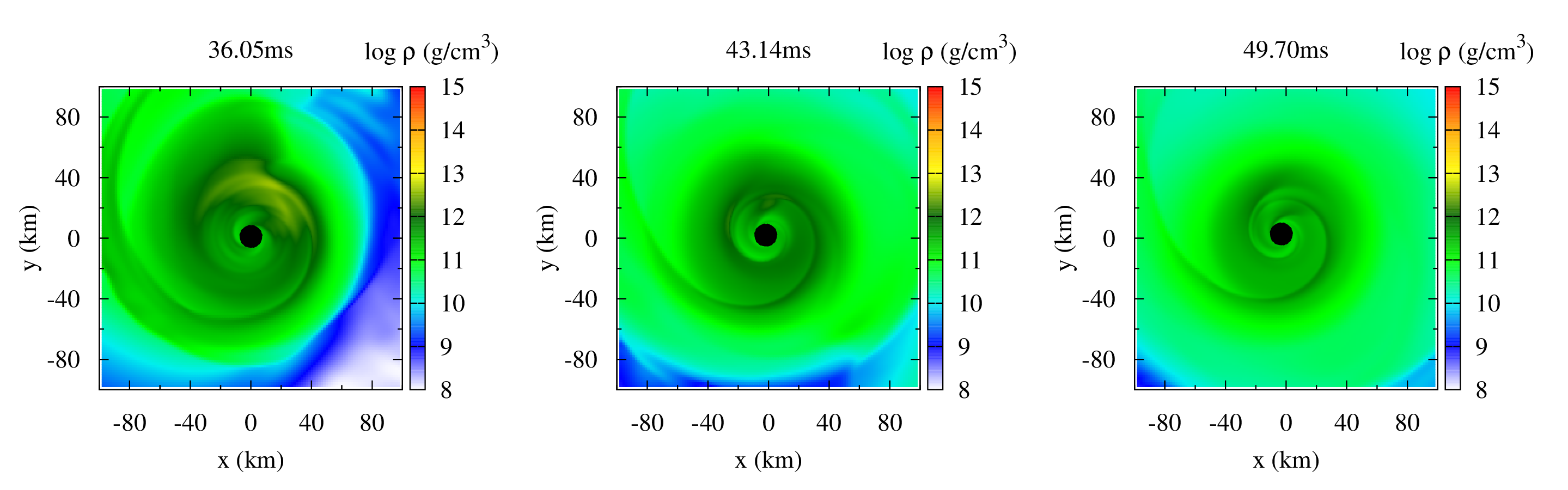
Figure 19: The same as Fig. 1 (H4-Q5a75) but at different time slices.

One feature of remnant disks overlooked in our previous studies is the existence of standing spiral accretion shocks. Figure 19 shows rest-mass density profiles on the equatorial plane in the central region at different time slices for H4-Q5a75. This figure (see also the right panel of Fig. 1) shows that sharp spirals extending to the apparent horizon stay in approximately the same location over $10\text{\,}\mathrm{ms}$ without exhibiting any rotation. Similar structures are found for most of the models as long as the remnant disk is appreciable, and we find no cases in which this spiral structure disappears by the end of simulations, which is at $\gtrsim$50\text{\,}\mathrm{ms}$$ after the onset of merger for the longest runs. The standing spiral shocks appear to be formed as a trace of self-collision of tidal tails rather than as a result of disk instability. This spiral structure should serve to dissipate the angular momentum of disk material and enhance mass accretion by the remnant black hole.

Table 4: Characteristic physical quantities associated with the remnant black hole measured at $10\text{\,}\mathrm{ms}$ after the merger and with gravitational waves for our fiducial, $N=60$ runs. $M_{\mathrm{BH,f}}$ and $\chi_{\mathrm{f}}$ are the mass and dimensionless spin parameter, respectively, of the remnant black hole. $V_{\mathrm{ej}}$ and $V_{\mathrm{GW}}$ are the magnitude of velocities imparted to the remnant black hole-disk system due to the ejecta backreaction and gravitational-wave recoil, respectively. $\Delta E_{\mathrm{GW}}$ and $\Delta J_{\mathrm{GW}}$ are the energy and angular momentum, respectively, radiated by gravitational waves.

Model	$M_{\mathrm{BH,f}}[M_{\odot}]$	$\chi_{\mathrm{f}}$	$V_{\mathrm{ej}}$ ($\mathrm{km}\text{\,}{\mathrm{s}}^{-1}$)	$V_{\mathrm{GW}}$ ($\mathrm{km}\text{\,}{\mathrm{s}}^{-1}$)	$\Delta E_{\mathrm{GW}}[M_{\odot}]$	$\Delta J_{\mathrm{GW}}[M_{\odot}^{2}]$
APR4-Q3a75	5.07	0.87	100	90	$9.3\text{\times}{10}^{-2}$	5.6
ALF2-Q3a75	5.02	0.86	500	60	$6.3\text{\times}{10}^{-2}$	4.6
H4-Q3a75	4.99	0.88	500	60	$4.9\text{\times}{10}^{-2}$	4.0
MS1-Q3a75	4.97	0.88	800	20	$4.0\text{\times}{10}^{-2}$	3.5
APR4-Q3a5	5.17	0.77	20	70	$9.2\text{\times}{10}^{-2}$	5.3
ALF2-Q3a5	5.10	0.76	300	70	$6.1\text{\times}{10}^{-2}$	4.3
H4-Q3a5	5.07	0.76	300	50	$4.8\text{\times}{10}^{-2}$	3.7
MS1-Q3a5	5.05	0.75	600	50	$3.9\text{\times}{10}^{-2}$	3.3
APR4-Q3a0	5.26	0.55	$<1$	60	$8.2\text{\times}{10}^{-2}$	4.3
ALF2-Q3a0	5.26	0.56	20	30	$6.1\text{\times}{10}^{-2}$	3.8
H4-Q3a0	5.20	0.55	70	40	$4.6\text{\times}{10}^{-2}$	3.2
MS1-Q3a0	5.16	0.53	200	40	$3.6\text{\times}{10}^{-2}$	2.8
APR4-Q5a75	7.80	0.85	30	20	0.16	10
ALF2-Q5a75	7.69	0.83	400	40	0.11	9.1
H4-Q5a75	7.65	0.83	400	70	$9.0\text{\times}{10}^{-2}$	8.0
MS1-Q5a75	7.62	0.83	700	50	$7.5\text{\times}{10}^{-2}$	7.2
APR4-Q5a5	7.90	0.71	$<1$	30	0.13	8.8
ALF2-Q5a5	7.89	0.71	30	30	0.11	8.3
H4-Q5a5	7.81	0.70	200	50	$8.9\text{\times}{10}^{-2}$	7.4
MS1-Q5a5	7.74	0.68	400	50	$7.2\text{\times}{10}^{-2}$	6.7
APR4-Q7a75	10.5	0.83	$<1$	40	0.17	14
ALF2-Q7a75	10.5	0.83	40	30	0.16	13
H4-Q7a75	10.4	0.82	200	40	0.13	12
MS1-Q7a75	10.3	0.81	400	30	0.11	11
APR4-Q7a5	10.6	0.67	$<1$	30	0.12	10
ALF2-Q7a5	10.6	0.67	$<1$	30	0.12	11
H4-Q7a5	10.6	0.67	6	20	0.11	10
MS1-Q7a5	10.6	0.67	30	20	0.10	9.9

The mass and dimensionless spin parameter of the remnant black holes at $10\text{\,}\mathrm{ms}$ after the onset of merger are listed in Table 4. They are consistent with our previous results for models with comparable binary parameters Kyutoku et al. (2010, 2011b, 2011a). After the measurement, the dimensionless spin parameters increase by up to $\approx 0.01$ due to long-term accretion depending on the models. Thus, the values of $\chi_{\mathrm{f}}$ shown in Table 4 may be regarded as the lower limits of hypothetical final configurations which will be achieved by purely hydrodynamic processes.

The remnant black hole-disk system including fallback material receives a recoil velocity due to the backreaction of anisotropic mass ejection Rosswog et al. (2000); Kyutoku et al. (2013), which we call the ejecta kick velocity. The ejecta kick velocity, $V_{\mathrm{ej}}$, is estimated by linear-momentum conservation as

$$V_{\mathrm{ej}} \approx\frac{P_{\mathrm{ej}}}{m_{0}}$$

$$=$555\text{\,}\mathrm{km}\text{\,}{\mathrm{s}}^{-1}$\;\left(\frac{P_{\mathrm{ej}}}{0.01M_{\odot}}\right)\left(\frac{Q+1}{4}\right)^{-1},$$ (41)

where $M_{\mathrm{NS}}=1.35M_{\odot}$ is assumed. For simplicity, the mass of the remnant black hole-disk system is approximated by $m_{0}$ in this expression, neglecting energy loss to the ejecta and to gravitational waves. The former is $\lesssim 0.02m_{0}$, and the latter is $\lesssim 0.03m_{0}$ for the cases considered here, where the energy radiated during the very early inspiral phase that existed before our initial condition, $m_{0}-M_{0}$, is also taken into account. Because the ejecta mass is large only when tidal disruption occurs at a distant orbit and gravitational radiation is not very strong, the sum of both does not exceed $0.03m_{0}$.

Values of the ejecta kick velocity for each model are presented in Table 4. This table shows that $V_{\mathrm{ej}}$ can be several hundreds of $\mathrm{km}\text{\,}{\mathrm{s}}^{-1}$ when mass ejection is efficient and easily dominates kick velocities due to the gravitational radiation reaction, $V_{\mathrm{GW}}$, which we discuss in Sec. III.7.

III.7 Gravitational waves

Gravitational waves from black hole-neutron star binaries are thoroughly investigated in our previous work Kyutoku et al. (2010, 2011b, 2011a), and derived waveforms are used to construct phenomenological models aiming at data analysis Lackey et al. (2012); Pannarale et al. (2013); Lackey et al. (2014). In the following, we instead discuss integrated or instantaneous properties of gravitational waves.

The energy, linear momentum, and angular momentum carried away by gravitational waves are presented in Table 4. While the energy $\Delta E_{\mathrm{GW}}$ and the angular momentum $\Delta J_{\mathrm{GW}}$ are presented as they are, the magnitude of linear momentum $\Delta P_{\mathrm{GW}}$ is shown instead as the velocity imparted to the remnant black hole-disk system including fallback material,

$$V_{\mathrm{GW}}\approx\frac{\Delta P_{\mathrm{GW}}}{m_{0}},$$ (42)

where we adopt $m_{0}$ as in Eq. (41). We call $V_{\mathrm{GW}}$ the gravitational-wave kick velocity. Although the accuracy in computing $\Delta P_{\mathrm{GW}}$ is not very high due to mode couplings, we do not find $V_{\mathrm{GW}}$ larger than $100\text{\,}\mathrm{km}\text{\,}{\mathrm{s}}^{-1}$ for the models considered in this study. Broadly speaking, the ejecta kick velocity, $V_{\mathrm{ej}}$, dominates the gravitational-wave kick velocity, $V_{\mathrm{GW}}$, when $M_{\mathrm{ej}}\gtrsim 0.01M_{\odot}$.

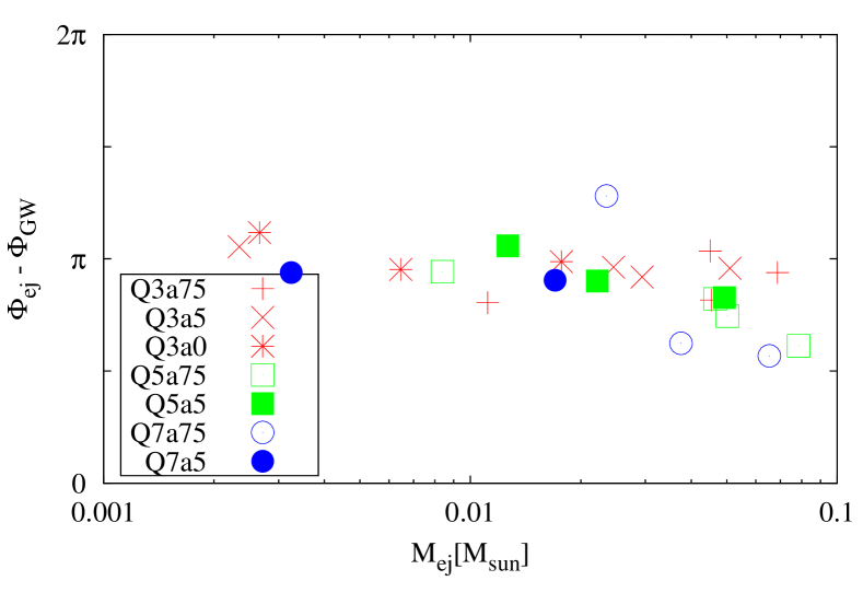
Figure 20: Difference between the angle of ejecta linear momentum, $\Phi_{\mathrm{ej}}$, and of gravitational-wave linear momentum, $\Phi_{\mathrm{GW}}$, vs the ejecta mass, $M_{\mathrm{ej}}$. We restrict the range to $M_{\mathrm{ej}}\geq 0.001M_{\odot}$.

The ejecta kick velocity and gravitational-wave kick velocity partially cancel out each other, because their angles $\Phi_{\mathrm{ej}}$ and $\Phi_{\mathrm{GW}}$ point in approximately opposite directions. Figure 20 shows the difference between them, $\Phi_{\mathrm{ej}}-\Phi_{\mathrm{GW}}$, vs $M_{\mathrm{ej}}$. The differences cluster around $\pi$ irrespective of the model parameters, and this means that ejecta and gravitational waves carry linear momenta in opposite directions. This tendency does not depend on grid resolutions. While the origin of anticorrelation is nontrivial, it is reasonable that $\Phi_{\mathrm{ej}}-\Phi_{\mathrm{GW}}$ prefers a specific value, because both dynamical mass ejection and linear-momentum emission are determined primarily by merger dynamics including tidal disruption. The largest velocity in the coalescence event is achieved by the plunge motion of material promptly swallowed by the black hole after the tidal disruption, and the plunge should emit the linear momentum efficiently in its direction due to the large velocity (see Refs. Wiseman (1992); Blanchet et al. (2005) for relevant discussions). A possible explanation of the anticorrelation between $\Phi_{\mathrm{ej}}$ and $\Phi_{\mathrm{GW}}$ is that the linear momentum is emitted right after the tidal disruption primarily in the direction of the plunge motion, which should be opposite to the ejecta motion. This anticorrelation implies that the realistic value of the remnant velocity is given approximately by $|V_{\mathrm{ej}}-V_{\mathrm{GW}}|$.

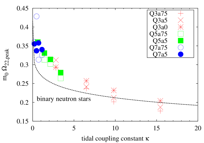
Figure 21: Dimensionless gravitational-wave frequency of $(2,2)$ mode gravitational waves, $m_{0}\Omega_{22,\mathrm{peak}}$, at the amplitude peak as a function of the tidal coupling constant $\kappa$ defined by Eq. (43). The dashed line is a fit obtained from binary neutron star simulations due to Ref. Read et al. (2013).

Finally, we comment on the possible existence of a tight correlation between the strength of tidal effects and gravitational-wave frequency at the maximum amplitude, which is suggested to exist for binary neutron stars Read et al. (2013); Bernuzzi et al. (2014). Figure 21 shows a dimensionless gravitational-wave frequency of the $(2,2)$ mode at the maximum amplitude, $m_{0}\Omega_{22,\mathrm{peak}}$, as a function of a tidal coupling constant,

$$\kappa=\frac{2Q}{(1+Q)^{5}}\frac{k}{\mathcal{C}^{5}}=\frac{3Q}{(1+Q)^{5}}\Lambda,$$ (43)

adapted to black hole-neutron star binaries Damour and Nagar (2010) (see also Ref. Vines et al. (2011)). This figure suggests the existence of relations independent of the mass ratio and equation of state. If the correlations are tight, it implies that the finite-size effect in the black hole-neutron star binary merger is described fairly well by the quadrupolar tidal deformability up to tidal disruption. These relations depend on the black-hole spin, and our results suggest that $m_{0}\Omega_{22,\mathrm{peak}}$ is smaller for a larger black-hole spin. This agrees with Ref. Bernuzzi et al. (2014). The same value of $\chi$ may not be compared directly among different mass ratios except for nonspinning cases, and effective spin parameters weighted by the mass ratio such as $\chi[1+3/(4Q)]Q^{2}/(1+Q)^{2}$ (see, e.g., Refs. Kidder et al. (1993); Damour (2001)) will be more appropriate. If such correlations are confirmed accurately by future simulations, they would help to extract neutron-star equations of state without detailed analysis of the phase evolution, just as knowledge of the cutoff frequency would do Vallisneri (2000); Shibata et al. (2009, 2012); Kyutoku et al. (2010, 2011b, 2011a).

Because the gravitational-wave amplitude peaks during the rapid increase of the frequency, the error of $m_{0}\Omega_{22,\mathrm{peak}}$ is not very small. Typical errors are estimated to be $\approx 5\%$ due to eccentricities, $\approx 10\%$ due to the finite resolution, and $\approx 5\%$ due to the gravitational-wave extraction method like extraction radii (even with the extrapolation). Hence, the total error may be $\approx 20\%$ in the worst case.

A relation satisfied by nonspinning black hole-neutron star binaries (if really exists) is not necessarily the same as that by binary neutron stars, because the merger dynamics is very different. We include a fitting curve derived from binary neutron star simulations Read et al. (2013) in Fig. 21. We cannot determine whether the relations are different or not from the current data by two reasons. One is the numerical error associated with each simulation. The other is the fact that tidal coupling constants, $\kappa$, spanned by binary neutron star simulations are much larger than those by black hole-neutron star binary simulations, and thus the extrapolated relations cannot be seriously trusted. Specifically, the relation derived in Ref. Read et al. (2013) is obtained by fitting results of simulations with $26\leq\kappa\leq 440$, none of which overlaps with that in our current simulations. It may be worth future investigation to test whether relations are distinct between binary neutron stars and nonspinning black hole-neutron star binaries.

IV Electromagnetic counterpart

In this section, we discuss expected characteristics of electromagnetic counterparts based on the properties of dynamical ejecta derived by our simulations. We focus primarily on the effect of anisotropy, which is characterized by the opening angle in the equatorial plane, $\varphi_{\mathrm{ej}}$, and in the meridional plane, $\theta_{\mathrm{ej}}$, on the macronova/kilonova Li and Paczyński (1998); Kulkarni ; Metzger et al. (2010a); Kisaka et al. (2015) and synchrotron radio emission Nakar and Piran (2011); Takami et al. (2014a). A concise summary of the main results derived in this section is found in Ref. Kyutoku et al. (2013), in which other aspects of the ejecta like gravitational-wave memory emission and cosmic-ray acceleration are also discussed.

For simplicity, we adopt slightly different notations for ejecta quantities in this section from those in other sections. Specifically, we denote the ejecta mass by $M$ instead of $M_{\mathrm{ej}}$. The opening angles are denoted by $\theta$ and $\varphi$ instead of $\theta_{\mathrm{ej}}$ and $\varphi_{\mathrm{ej}}$, respectively. Recall that $\theta(=\theta_{\mathrm{ej}})$ is defined as the half-opening angle taking the equatorial symmetry into account, and a full sphere corresponds to $\theta=\pi/2$ and $\varphi=2\pi$. We also adopt short-hand notations $M_{-2}\equiv M/(0.01M_{\odot})$, $\theta_{i}\equiv\theta/(1/5)$, and $\varphi_{i}\equiv\varphi/\pi$. We recover the speed of light, $c$, everywhere.

IV.1 Macronova/kilonova

The macronova/kilonova is quasithermal radiation from the ejecta heated by the decay of unstable r-process elements. The dynamical ejecta from mergers of black hole-neutron star binaries will be composed primarily of neutrons as discussed in Sec. III.2.1, and then r-process elements should be synthesized Lattimer and Schramm (1974, 1976). After the neutrons are exhausted within a few seconds, $\beta$-decay and fission of unstable r-process elements heat the ejecta. The heated ejecta emit radiation primarily in red-optical and infrared bands on a day-to-month time scale Tanaka et al. (2014), where a bunch of Doppler-broadened lines associated with the complicated energy-level structure of r-process elements blanket the emission in blue-optical and ultraviolet bands Kasen et al. (2013); Tanaka and Hotokezaka (2013).

IV.1.1 Analytic model

Qualitative features of the macronova/kilonova from the anisotropic ejecta can be understood by modifying the prototypical model for spherical ejecta proposed in Ref. Li and Paczyński (1998). In this section, we introduce short-hand notations $V_{-1}\equiv V/(0.1c)$ for the surface velocity, $\kappa_{1}\equiv\kappa/($10\text{\,}{\mathrm{g}}^{-1}\text{\,}{\mathrm{cm}}^{2}$)$ for the opacity, and $f_{-6}\equiv f/${10}^{-6}$$ for the heating efficiency. The precise meaning of these quantities is explained in the following.

We approximate the hydrodynamic evolution of the ejecta by the free expansion of a uniform-density truncated sphere characterized by the opening angles $\theta$ and $\varphi$. The radius of the (truncated) sphere is given by $R(t)=Vt$ using the surface velocity $V$, and thus the rest-mass density of the ejecta is

$$\rho(t)=\frac{3\pi M}{4\theta\varphi V^{3}t^{3}}.$$ (44)

In this uniform-density free-expansion model, the surface velocity is related to the average velocity of the ejecta defined by Eq. (20) via $V=\sqrt{5/3}v_{\mathrm{ave}}\approx 1.3v_{\mathrm{ave}}$. Because the ejecta material is expected to be radiation-dominated in the relevant epoch due to r-process heating, the internal energy density $u$ is related to the pressure $P$ and temperature $T$ by $u=3P=aT^{4}$, where $a$ is the radiation constant. The time evolution of the internal energy density is derived by the first law of thermodynamics as

$$t^{3}\frac{du}{dt}+4t^{2}u=\frac{3\pi M}{4\theta\varphi V^{3}}\dot{\varepsilon}-\frac{3\pi}{4\theta\varphi V^{3}}L,$$ (45)

where $\dot{\varepsilon}$ is the specific heating rate and $L$ is the luminosity. Time-dependent quantities are $u$, $\dot{\varepsilon}$, and $L$.

We assume that the specific heating rate is given by a power law $\dot{\varepsilon}(t)=fc^{2}/t$ parametrized by the heating efficiency $f$ in the same manner as the spherical model Li and Paczyński (1998). An appropriate value of the heating efficiency, $f$, will depend significantly on the electron fraction (the number of electrons per baryon) Rosswog et al. (2014); Wanajo et al. (2014). The uncertainty is particularly high when fission is an important heating source rather than $\beta$-decay of elements near the stability line Wanajo et al. (2014). In this study, we take the fiducial value of $f$ to be ${10}^{-6}$ following Ref. Wanajo et al. (2014).

We give the luminosity by a diffusion approximation in a similar manner to the spherical model Li and Paczyński (1998) but assuming geometry adapted to anisotropic mass ejection. The assumption is that the radiation is emitted not from the truncated spherical surface but from the cross section of truncation. In the language of our simulations, photons from the anisotropic ejecta are assumed to escape mainly into the $\pm z$ directions, and the emitting surfaces are taken to be those observed from the $\pm z$ direction like ones depicted in Fig. 6. The temperature gradient $dT/dr$ relevant to the diffusion flux is approximated by $\approx T/(\theta R)$ rather than $\approx T/R$ of the spherical ejecta under this assumption. Thus, the flux may be given by

$$F(t)\approx\frac{\sigma_{\mathrm{SB}}T^{4}}{\kappa\rho\theta R},$$ (46)

where $\kappa$ is the opacity and $\sigma_{\mathrm{SB}}$ is the Stefan–Boltzmann constant. In this estimation, a factor of order unity is neglected in exactly the same manner as in Ref. Li and Paczyński (1998). The emitting area is then given approximately by $2\times\varphi R^{2}/2=\varphi R^{2}$, where the first “2” stands for two emitting surfaces at $+z$ and $-z$, and therefore the bolometric luminosity may be given by

$$L(t)\approx\frac{\varphi^{2}V^{4}c}{3\pi\kappa M}t^{4}u.$$ (47)

This expression does not reduce to that for the spherical ejecta even if we adopt $\theta=\pi/2$ and $\varphi=2\pi$ because of different assumptions. The neglected truncated spherical surface has the area $(4/\pi)\theta\varphi R^{2}$, and thus the luminosity may be underestimated by a fraction of $(4/\pi)\theta\approx 30\%$. Although this term can be included with no difficulty, we omit this contribution so that the parameter dependence becomes clear.

The value of opacity, $\kappa$, is highly uncertain due to our incomplete knowledge of r-process elements and their line features Kasen et al. (2013); Tanaka and Hotokezaka (2013). Although the realistic opacity of r-process elements is safely assumed to be dominated by various bound-bound transition lines in optical and ultraviolet wavelengths, no complete line list exists so far. In this study, we take the fiducial value of $\kappa$ to be $10\text{\,}{\mathrm{g}}^{-1}\text{\,}{\mathrm{cm}}^{2}$, because this approximately reproduces results obtained by radiation transfer simulations performed adopting currently available line lists Tanaka and Hotokezaka (2013). The gray approximation adopted in this model is not realistic and limits the predictability of the spectra.

The thermodynamic evolution equation can be solved analytically. For this purpose, it is convenient to cast the equation into a dimensionless form. First, we normalize the surface velocity by the speed of light as $\beta_{s}\equiv V/c$ in the usual manner. Next, we define a characteristic time scale by the condition that the optical depth of a characteristic path becomes unity, $\kappa\rho\theta R=1$, and this gives a critical time of the onset of transparency,

$$t_{c}=\sqrt{\frac{3\pi\kappa M}{4\varphi V^{2}}}\;.$$ (48)

Finally, a characteristic internal energy density can be defined by

$$u_{c}=f\rho(t_{c})c^{2}=\sqrt{\frac{4\varphi f^{2}c^{4}}{3\pi\kappa^{3}\theta^{2}M}}\;.$$ (49)

Introducing dimensionless variables $\tilde{t}=t/t_{c}$ and $\tilde{u}=u/u_{c}$, we obtain the dimensionless evolution equation,

$$\frac{d\tilde{u}}{d\tilde{t}}+\left(\frac{4}{\tilde{t}}+\frac{3\pi\tilde{t}}{16\theta\beta_{s}}\right)\tilde{u}=\frac{1}{\tilde{t}^{4}},$$ (50)

which has an analytic solution

$$\tilde{u}(t)=\frac{C}{\tilde{t}^{4}}\exp\left(-\frac{3\pi\tilde{t}^{2}}{32\theta\beta_{s}}\right)+\sqrt{\frac{32\theta\beta_{s}}{3\pi}}\frac{1}{\tilde{t}^{4}}Y\left(\sqrt{\frac{3\pi}{32\theta\beta_{s}}}\tilde{t}\right),$$ (51)

where $C$ is the integration constant and $Y$ is Dawson’s integral defined by

$$Y(x)\equiv e^{-x^{2}}\int_{0}^{x}e^{s^{2}}ds.$$ (52)

Because the initial internal energy of the ejecta is rapidly lost due to the adiabatic cooling, we may safely set the integration constant, $C$, to be zero. The key issue which allows us to derive this analytic solution for nonspherical ejecta is that the temporal dependence of each term (adiabatic cooling, radiative cooling, and heating) is not affected by the geometry in our model.

The peak time, peak bolometric luminosity, and effective temperature at the peak time can be estimated using this solution. Note that Dawson’s integral takes the maximum value $y_{p}\approx 0.54$ at $x_{p}\approx 0.92$. The peak time is

$$t_{\mathrm{peak}} =x_{p}\sqrt{\frac{8\kappa\theta M}{\varphi Vc}}$$

$$=$11\text{\,}\mathrm{d}\mathrm{a}\mathrm{y}$\;\kappa_{1}^{1/2}M_{-2}^{1/2}V_{-1}^{-1/2}\theta_{i}^{1/2}\varphi_{i}^{-1/2}.$$ (53)

The peak bolometric luminosity is

$$L_{\mathrm{peak}} =y_{p}\sqrt{\frac{\varphi f^{2}MVc^{5}}{2\theta\kappa}}$$

$$=$1.8\text{\times}{10}^{40}\text{\,}\mathrm{e}\mathrm{r}\mathrm{g}\,\mathrm{c}\mathrm{m}^{-3}$\;f_{-6}\kappa_{1}^{-1/2}M_{-2}^{1/2}V_{-1}^{1/2}\theta_{i}^{-1/2}\varphi_{i}^{1/2}.$$ (54)

The effective temperature is defined from the diffusion flux, Eq. (46), by $T_{\mathrm{eff}}\equiv(F/\sigma_{\mathrm{SB}})^{1/4}$, and its value at the peak time is

$$T_{\mathrm{peak}} =\frac{y_{p}^{1/4}}{x_{p}^{1/2}}\left(\frac{\varphi f^{2}c^{5}}{8a^{2}\theta^{3}\kappa^{3}MV}\right)^{1/8}$$

$$=$1900\text{\,}\mathrm{K}$\;f_{-6}^{1/4}\kappa_{1}^{-3/8}M_{-2}^{-1/8}V_{-1}^{-1/8}\theta_{i}^{-3/8}\varphi_{i}^{1/8}.$$ (55)

These expressions share the same parameter dependence as those derived in Ref. Kyutoku et al. (2013) by random-walk arguments. This indicates that the parameter dependence is robust as far as similar assumptions are adopted.

In the range of opening angles observed in our numerical simulations, the macronova/kilonova from black hole-neutron star binaries tends to peak slightly earlier with slightly higher bolometric luminosity than that from the spherical ejecta for given values of other parameters. This tendency is also observed in radiation transfer simulations Tanaka et al. (2014). When the opening angle in the meridional plane, $\theta$, is small, the peak time becomes early and the peak bolometric luminosity increases. The reason for this is that photons can escape easily from the ejecta when $\theta$ is small. Specifically, the optical depth $\kappa\rho\theta R$ at $t_{\mathrm{peak}}$ is proportional to $\theta^{-1}$ and independent of $\varphi$. When the opening angle in the equatorial plane, $\varphi$, is small, the peak time becomes late and the peak bolometric luminosity decreases. The reason is that a small value of $\varphi$ increases the rest-mass density, optical depth, and characteristic time scales. The dependence of luminosity may be understood by the constancy of $L_{\mathrm{peak}}t_{\mathrm{peak}}$ for both cases. The combined effects of these two angles tend to prefer the slightly earlier peak with slightly brighter emission. When the ejecta becomes transparent, the bolometric luminosity does not depend on the geometry, because we simply have $L=\dot{\varepsilon}M$ even within this model derived with the diffusion approximation.

At a given time, the material temperature $T$ and effective temperature $T_{\mathrm{eff}}$ are higher for the anisotropic ejecta than for the spherical one due to different geometry. In typical situations, the material temperature, $T$, is higher by about a factor of 2, and this agrees approximately with the result of Ref. Tanaka et al. (2014). The reason of the high temperature is that the decay heat of unstable r-process elements is deposited to a small volume for a given mass and velocity of the ejecta. Accordingly, the effective temperature, $T_{\mathrm{eff}}$, is higher by $\approx 30\%$–50%. Even this amount of difference could have a significant effect on the observed flux [not to be confused with the diffusion flux, Eq. (46), which is trivially related to $T_{\mathrm{eff}}$] in optical and near-infrared bands, because the typical value of $T_{\mathrm{peak}}$ is in the infrared band. Thus, a small increase of $T_{\mathrm{eff}}$ could enhance the flux at optical and near-infrared bands. In fact, we see that absolute/apparent magnitudes increase by 1–2 in these bands if we assume a perfect blackbody spectrum. We do not, however, regard this amount of increase as very quantitative, because realistic spectra will be very different from the blackbody. The high temperature could also affect possible dust formation Takami et al. (2014b).

The dependence of the peak quantities on $f$, $\kappa$, $M$, and $V$ is the same as that of the spherical model Li and Paczyński (1998). A large value of $f$ increases the luminosity, a large value of $\kappa$ delays the peak and decreases the luminosity, a large value of $M$ delays the peak and increases the luminosity, and a large value of $V$ hastens the peak and increases the luminosity. Among these parameters, the ejecta mass can become much larger for black hole-neutron star binaries than for binary neutron stars Hotokezaka et al. (2013a), and higher luminosity could be achieved Hotokezaka et al. (2013b). In fact, this difference may dominate corrections due to the opening angles. Typical velocities of the ejecta cannot be very different. The heating efficiency and opacity could change reflecting different compositions of the ejecta, but we do not discuss them in this study.

IV.1.2 Directional dependence, line, and polarization

We briefly discuss possible aspects of the macronova/kilonova from anisotropic ejecta that cannot be captured in the analytic model developed above. An obvious outcome of the anisotropy is the directional dependence (see Refs. Roberts et al. (2011); Grossman et al. (2014) for binary neutron stars). Emission should be brighter when observed from the direction perpendicular to the equatorial plane than in the equatorial plane. Specifically, the flux will be larger by $1/\theta\approx 3$–5 near $t_{\mathrm{peak}}$ for the former situation. Accordingly, the light curves will exhibit different evolution near $t_{\mathrm{peak}}$ and become indistinguishable after the entire ejecta becomes transparent. These behaviors are observed in radiation transfer simulations Tanaka et al. (2014). Followup observations of electromagnetic counterparts will benefit from this directional dependence, because gravitational waves are emitted most strongly in the direction perpendicular to the equatorial plane, in which the macronova/kilonova will be the brightest. That is, observed binaries will be biased toward the brightest direction of the macronova/kilonova.

A chance to observe spectral lines associated with r-process elements will be better for black hole-neutron star binaries than for binary neutron stars. In any case, it will be very challenging to observe such lines from the macronova/kilonova, because a bunch of lines are expected to be significantly blended due to Doppler broadening in the ejecta with a large surface velocity. This broadening may be mitigated in the direction perpendicular to the equatorial plane, because the expansion velocity is smaller by a factor of $\theta$ than in other directions and spherical cases. Furthermore, the emission is expected to be the brightest in this direction. Thus, the macronova/kilonova associated with black hole-neutron star binaries would deserve detailed spectroscopic observations to seek a (serendipitous) strong and isolated line (see also Ref. Kasen et al. (2013) for relevant discussions).

Potential diagnostics of the anisotropic geometry is polarization induced by electron scattering, but the polarization degree is not likely to be high for the macronova/kilonova. If the optical depth to electron scattering is sufficiently high and lines do not contribute to depolarization significantly, the linear polarization observed from the equatorial plane would be 4%–5% because of the highly deformed photosphere Höflich (1991). However, the number density of free electrons will be much smaller in the ejecta composed of r-process elements than in, e.g., the supernova ejecta near the peak luminosity. While the r-process elements have the mass number $\gtrsim 100$, the ionization degree will not be particularly high around the peak of the macronova/kilonova Kasen et al. (2013); Tanaka and Hotokezaka (2013). Hence, the opacity for the electron scattering will be lower by about 3 orders of magnitude than that for bound-bound transitions if $\kappa=$10\text{\,}{\mathrm{g}}^{-1}\text{\,}{\mathrm{cm}}^{2}$$ is an appropriate representative. The optical depth to electron scattering will be only $O(10^{-2})$ near $t_{\mathrm{peak}}$ when the total optical depth is at most $O(10)$, and therefore the polarization degree may be reduced by a similar factor. In addition, interaction with lines will further depolarize the radiation Jeffery (1989).

IV.2 Synchrotron radio emission

Nonthermal radiation such as synchrotron emission is expected to arise from blast waves formed between the ejecta and ambient interstellar medium in a similar manner to the supernova remnant and gamma-ray burst afterglow Nakar and Piran (2011); Takami et al. (2014a). Subrelativistic blast waves will develop as the ejecta sweeps the interstellar medium, and the kinetic energy of the ejecta is converted to postshock internal energy. A fraction of the internal energy at the forward shock will be converted to energy of nonthermal electrons assembled from the interstellar medium and of amplified magnetic fields. The accelerated electrons will radiate synchrotron emission in a magnetized environment, and the emission would be observed in radio bands Nakar and Piran (2011); Piran et al. (2013) and possibly in optical, x-ray, and $\gamma$-ray bands Takami et al. (2014a).

IV.2.1 Radiation at the deceleration time

The most luminous emission is expected when the ejecta begins to be decelerated significantly, and the deceleration time $t_{\mathrm{dec}}$ depends on the ejecta geometry for a given mass and velocity of the ejecta. We describe the synchrotron radio emission expected at $t_{\mathrm{dec}}$ adopting a simplified version of the nonrelativistic model developed in Ref. Takami et al. (2014a) (see also Ref. Ioka and Mészáros (2005)). We do not, however, attempt to model the time evolution in this study, because the lateral expansion should become important after the deceleration time for the anisotropic ejecta. While the late-time evolution of the spherical ejecta will be described reasonably by Sedov–Taylor’s self-similar solution as in Ref. Piran et al. (2013), it is difficult to formulate the lateral expansion of the anisotropic ejecta in a simple manner. We introduce short-hand notations $v_{-1}\equiv v/(0.1c)$ for the ejecta velocity, $n_{0}\equiv n/($1\text{\,}{\mathrm{cm}}^{-1}\text{\,}{\mathrm{}}^{3}$)$ for the ambient number density, $\epsilon_{\mathrm{e},-1}\equiv\epsilon_{\mathrm{e}}/0.1$ for the fraction of postshock internal energy given to nonthermal electrons, $\epsilon_{B,-1}\equiv\epsilon_{B}/0.1$ for the fraction of postshock internal energy given to magnetic fields, and $D_{2}\equiv D/($100\text{\,}\mathrm{M}\mathrm{p}\mathrm{c}$)$ for the distance from the observer to the site of binary coalescence. We also introduce the fraction $\eta$ of accelerated electrons and power-law index $p$ of the Lorentz factor distribution.

The ejecta is decelerated significantly when the mass comparable to its own is assembled from the interstellar medium. The deceleration radius of the anisotropic ejecta is given by

$$R_{\mathrm{dec}} =\left(\frac{3\pi M}{4\theta\varphi nm_{\mathrm{p}}}\right)^{1/3}$$

$$=$1.1\text{\,}\mathrm{p}\mathrm{c}$\;n_{0}^{-1/3}M_{-2}^{1/3}\theta_{i}^{-1/3}\varphi_{i}^{-1/3},$$ (56)

where $m_{\mathrm{p}}$ is the proton mass and $n$ is the number density of the ambient medium. Modeling the ejecta by a single-velocity shell with $v$, the corresponding deceleration time is

$$t_{\mathrm{dec}} =\frac{R_{\mathrm{dec}}}{v}$$

$$=$38\text{\,}\mathrm{y}\mathrm{e}\mathrm{a}\mathrm{r}$\;n_{0}^{-1/3}M_{-2}^{1/3}v_{-1}^{-1}\theta_{i}^{-1/3}\varphi_{i}^{-1/3}.$$ (57)

Here, the ejecta velocity, $v$, may be identified with the average velocity of the ejecta, $v_{\mathrm{ave}}$, defined by Eq. (20). The value of the ambient density, $n$, should vary by orders of magnitude depending on the location of the binary coalescence, and we normalize it by the typical value of the Galactic disk, $1\text{\,}{\mathrm{cm}}^{-3}$, following previous work Nakar and Piran (2011); Piran et al. (2013); Takami et al. (2014a). These expressions reduce to values for the spherical ejecta when we set $\theta=\pi/2$ and $\varphi=2\pi$.

If the typical opening angles observed in numerical simulations are kept until the deceleration time, $R_{\mathrm{dec}}$ and $t_{\mathrm{dec}}$ are larger by a factor of 2–3 than those for the spherical ejecta for given values of the other parameters. The reason for this is that only a limited fraction of the volume inside $R_{\mathrm{dec}}$ is swept by the anisotropic ejecta. Whereas the ejecta will approach a spherical state to some extent before $t_{\mathrm{dec}}$ Rosswog et al. (2014), the synchrotron radio emission from black hole-neutron star binaries will be a longer-lasting event than that for binary neutron stars.

The geometry does not modify the Lorentz factor distribution of nonthermal electrons and magnetic fields. The number of assembled electrons at $t_{\mathrm{dec}}$ is given by

$$N_{\mathrm{e,tot}} =\frac{M}{m_{\mathrm{p}}}$$

$$=$1.2\text{\times}{10}^{55}$\;M_{-2}.$$ (58)

Assuming that a fraction $\eta\leq 1$ of these electrons is accelerated to power-law distribution of the Lorentz factor $\gamma_{\mathrm{e}}$ with the index $p>2$ as

$$\frac{dN_{\mathrm{e}}(\gamma_{\mathrm{e}})}{d\gamma_{\mathrm{e}}}\propto\gamma_{\mathrm{e}}^{-p}\;(\gamma_{m}<\gamma_{\mathrm{e}}),$$ (59)

the minimum Lorentz factor may be derived from the number and energy of accelerated electrons as

$$\gamma_{m} =\frac{\epsilon_{\mathrm{e}}}{\eta}\frac{p-2}{p-1}\frac{m_{\mathrm{p}}}{m_{\mathrm{e}}}\frac{(v/c)^{2}}{2}$$

$$=0.92\;g(p)\eta^{-1}\epsilon_{\mathrm{e},-1}v_{-1}^{2},$$ (60)

where $m_{\mathrm{e}}$ is the electron mass, $\epsilon_{\mathrm{e}}$ is the fraction of the postshock internal energy given to the accelerated nonthermal electrons, and $g(p)\equiv(p-2)/(p-1)$. Care must be taken in applying this equation to subrelativistic blast waves, because $\gamma_{m}$ can fall below unity and become unphysical, particularly when the ejecta is significantly decelerated (not considered here). The strength of magnetic fields is given by

$$B =\sqrt{9\pi\epsilon_{B}nm_{\mathrm{p}}}v$$

$$=$6.5\text{\,}\mathrm{m}\mathrm{G}\mathrm{a}\mathrm{u}\mathrm{s}\mathrm{s}$\;\epsilon_{B,-1}^{1/2}n_{0}^{1/2}v_{-1},$$ (61)

where $\epsilon_{B}$ is the fraction of postshock internal energy converted to magnetic fields.

Parameters characterizing microphysics, $p$, $\eta$ , $\epsilon_{\mathrm{e}}$, and $\epsilon_{B}$, are all uncertain. Following Ref. Piran et al. (2013), we normalize $\epsilon_{\mathrm{e}}$ and $\epsilon_{B}$ by 0.1 and take the fiducial value of $p$ to be 2.5, which gives $g(p)=1/3$. Typical values of $p$ observed in nonrelativistic blast waves may be 2.5–3 Chevalier and Fransson (2006). The fiducial value of $\eta$ is set to be unity. Detailed spectroscopic observations of nonthermal radiation could determine these parameters in principle Takami et al. (2014a).

Quantities characterizing the instantaneous spectrum are estimated as follows. The synchrotron frequency of an electron with $\gamma_{\mathrm{e}}$ is defined by $\nu_{\mathrm{e}}(\gamma_{\mathrm{e}})\equiv qB\gamma_{\mathrm{e}}^{2}/(2\pi m_{\mathrm{e}}c)$, where $q$ is the elementary charge, and the power of the electron is by $P_{\mathrm{e}}(\gamma_{\mathrm{e}})\equiv\sigma_{\mathrm{T}}cB^{2}\gamma_{\mathrm{e}}^{2}/(6\pi)$, where $\sigma_{\mathrm{T}}$ is the Thomson cross section. The specific flux from a single electron at its peak frequency, $\nu_{\mathrm{e}}$, is estimated to be $P_{\nu}\approx P_{\mathrm{e}}/\nu_{\mathrm{e}}=\sigma_{\mathrm{T}}m_{\mathrm{e}}c^{2}B/(3q)$ independently from the electron Lorentz factor. The characteristic frequency of the electron distribution corresponding to $\gamma_{m}$ is given by

$$\nu_{m}=$1.5\text{\times}{10}^{4}\text{\,}\mathrm{Hz}$\;g(p)^{2}\eta^{-2}\epsilon_{\mathrm{e},-1}^{2}\epsilon_{B,-1}^{1/2}n_{0}^{1/2}v_{-1}^{5}.$$ (62)

An unabsorbed specific flux, i.e., a hypothetical specific flux in the absence of self-absorption, at $\nu_{m}$ is estimated to be

$$F_{\nu,m} =\frac{\eta N_{\mathrm{e,tot}}P_{\nu}}{4\pi D^{2}}$$

$$=$2.4\text{\,}\mathrm{J}\mathrm{y}$\;\eta\epsilon_{B,-1}^{1/2}n_{0}^{1/2}M_{-2}v_{-1}D_{2}^{-2},$$ (63)

where $D$ is the distance from the observer to the site of binary coalescence. If we neglect synchrotron self-absorption and cooling, the specific flux is given by $F_{\nu,m}(\nu/\nu_{m})^{1/3}$ below $\nu_{m}$ and $F_{\nu,m}(\nu/\nu_{m})^{-(p-1)/2}$ above $\nu_{m}$. We show below that the self-absorption could suppress the radio spectrum, while the cooling is not important in the radio band.

The self-absorption frequency $\nu_{a}$ may be obtained approximately by comparing the hypothetical unabsorbed flux with the blackbody flux in the Rayleigh regime Ioka and Mészáros (2005). The blackbody flux at $\nu_{m}$ is given by

$$F_{\nu,\mathrm{BB}}=2\pi\nu_{m}^{2}\gamma_{m}m_{\mathrm{e}}\frac{A_{\mathrm{em}}}{4\pi D^{2}},$$ (64)

where $A_{\mathrm{em}}$ is the blackbody emitting area. While this should be $4\pi R_{\mathrm{dec}}^{2}$ for the spherical ejecta, we take $A_{\mathrm{em}}=\varphi R_{\mathrm{dec}}^{2}\propto\theta^{2/3}\varphi^{-1/3}$ for the anisotropic ejecta in a similar manner to Sec. IV.1.1. It is readily found that $\nu_{m}<\nu_{a}$ when $F_{\nu,\mathrm{BB}}<F_{\nu,m}$, and vice versa. The case that $\nu_{m}<\nu_{a}$ is typical for subrelativistic blast waves, and the self-absorption frequency is defined as the frequency at which the synchrotron and blackbody fluxes are equal. Specifically, we obtain

$$\nu_{a} =\left(\frac{F_{\nu,m}}{F_{\nu,\mathrm{BB}}}\right)^{2/(4+p)}\nu_{m}$$

$$=$3.9\text{\times}{10}^{7}\text{\,}\mathrm{Hz}$\;\eta^{-2(p-2)/(4+p)}$$

$$\times\epsilon_{\mathrm{e},-1}^{2(p-1)/(4+p)}\epsilon_{B,-1}^{(2+p)/[2(4+p)]}n_{0}^{(14+3p)/[6(4+p)]}$$

$$\times M_{-2}^{2/[3(4+p)]}v_{-1}^{(5p-2)/(4+p)}\theta_{i}^{4/[3(4+p)]}\varphi_{i}^{-2/[3(4+p)]},$$ (65)

where the prefactor is given for $p=2.5$ and varies by a factor of 2 within $2.1<p<3$. The dependence on the opening angles is inherited from the emitting area, $A_{\mathrm{em}}$, and $\nu_{a}$ is smaller by a few tens of percent for the anisotropic ejecta than for the spherical one. The self-absorption frequency can increase to $\sim$1\text{\,}\mathrm{GHz}$$ in a plausible parameter range, and thus the self-absorption could be important at low-frequency radio bands for such cases. When $\nu_{a}<\nu_{m}$, we instead obtain $\nu_{a}=(F_{\nu,m}/F_{\nu,\mathrm{BB}})^{3/5}\nu_{m}$.

The cooling Lorentz factor $\gamma_{c}$ at the deceleration time, above which the radiative energy loss plays a significant role, is estimated by the condition $\gamma_{c}m_{\mathrm{e}}c^{2}=P(\gamma_{c})t_{\mathrm{dec}}$, and we obtain

$$\gamma_{c} =\frac{6\pi m_{\mathrm{e}}c}{\sigma_{\mathrm{T}}B^{2}t_{\mathrm{dec}}}$$

$$=$1.5\text{\times}{10}^{4}$\;\epsilon_{B,-1}^{-1}n_{0}^{-2/3}M_{-2}^{-1/3}v_{-1}^{-1}\theta_{i}^{1/3}\varphi_{i}^{1/3}.$$ (66)

The corresponding cooling frequency is given by

$$\nu_{c}=$4.3\text{\times}{10}^{12}\text{\,}\mathrm{Hz}$\;\epsilon_{B,-1}^{-3/2}n_{0}^{-5/6}M_{-2}^{-2/3}v_{-1}^{-1}\theta_{i}^{2/3}\varphi_{i}^{2/3}.$$ (67)

Although the cooling frequency decreases by a factor of several for the anisotropic ejecta due to the long deceleration time, this could affect the radio spectrum at high frequency only in a limited parameter range.

Finally, the instantaneous spectrum for $\nu_{m}<\nu_{a}<\nu_{c}$ is given by

$$\frac{F_{\nu}}{F_{\nu,m}}=\begin{cases}(\nu_{a}/\nu_{m})^{-(p+4)/2}(\nu/\nu_{m})^{2}&(\nu<\nu_{m})\\ (\nu_{a}/\nu_{m})^{-(p-1)/2}(\nu/\nu_{a})^{5/2}&(\nu_{m}\leq\nu<\nu_{a})\\ (\nu/\nu_{m})^{-(p-1)/2}&(\nu_{a}\leq\nu<\nu_{c})\\ (\nu_{c}/\nu_{m})^{-(p-1)/2}(\nu/\nu_{c})^{-p/2}&(\nu_{c}\leq\nu)\end{cases}.$$ (68)

The third segment is the most relevant to radio observations, and it would be useful to reexpress the spectrum in this range as

$$F_{\nu} =$0.12\text{\,}\mathrm{m}\mathrm{J}\mathrm{y}$\;\left(\frac{\nu}{$1\text{\,}\mathrm{GHz}$}\right)^{-(p-1)/2}$$

$$\times\eta^{1-p}\epsilon_{\mathrm{e},-1}^{p-1}\epsilon_{B,-1}^{(p+1)/4}n_{0}^{(p+1)/4}M_{-2}v_{-1}^{(5p-3)/2}D_{2}^{-2},$$ (69)

where the prefactor is for $p=2.5$ and decreases by a factor of 40 as $p$ increases from 2.1 to 3. This expression indicates that the emission associated with the massive ejecta from black hole-neutron star binaries will be bright.

IV.2.2 Proper motion

Aside from the expansion, the anisotropic ejecta from black hole-neutron star binaries exhibits center-of-mass motion, and thus the proper motion of radio images could be observed Kyutoku et al. (2013). The characteristic distance of the center-of-mass motion may be given approximately by $R_{\mathrm{com}}=v_{\mathrm{ej}}t_{\mathrm{dec}}=R_{\mathrm{dec}}(v_{\mathrm{ej}}/v_{\mathrm{ave}})$. The projected distance on the celestial sphere should be smaller by a factor of $\approx 2$ due to the angular average, whereas the observational bias due to the directional dependence of gravitational radiation should mitigate this decrease. The expected amount of projected travel distances is $O(1)$ pc [see Eq. (56)], and we expect the radio image of the anisotropic ejecta to move $O(1)$ milliarcsecond during its bright emission for a event at $O(100)$ Mpc. This amount of proper motion could be resolved by current radio instruments depending on the parameters and observed frequency Taylor et al. (2004) and could help to distinguish black hole-neutron star binaries from binary neutron stars only by electromagnetic counterparts.

V Summary

We performed numerical-relativity simulations of black hole-neutron star binary mergers to study dynamical mass ejection. The mass ratio, black-hole spin, and neutron-star equation of state were systematically varied to reveal the dependence of the ejecta properties on these parameters. We found that dynamical mass ejection is driven primarily by the tidal torque exerted from black holes to elongated neutron stars, and this process progresses over $\approx$2\text{\,}\mathrm{ms}$$ after the onset of merger. The dynamical ejecta is concentrated around the equatorial plane with a half opening angle of $10\mathrm{°}$–$20\mathrm{°}$ and sweeps out about a half of the plane, except for cases that mass ejection is inefficient. Because of this anisotropy, the ejecta carries a bulk linear momentum, and thus the remnant black hole-disk system receives an ejecta kick velocity due to the backreaction.

The ejecta mass can be as large as $\sim 0.1M_{\odot}$, and the average velocity of the ejecta defined from the kinetic energy is typically 0.2–$0.3c$. Dynamical mass ejection tends to become efficient when the neutron-star compactness is small, the mass ratio is small, and/or the black-hole spin is large. The dependence of ejecta properties on the compactness, however, is not as simple as that of the total mass remaining outside the apparent horizon. This suggests that not only the compactness but also detailed properties of the equation of state influence the ejecta properties significantly. Furthermore, the dependence on the mass ratio is not always monotonic. The ratio of the ejecta mass to the bound mass is large when the mass ratio is large, and the average velocity of the ejecta is also large for such cases. These suggest that the dynamical ejecta from higher-mass-ratio binaries is more energetic for a given ejecta mass.

We also found that the bound envelope along the polar axis of the central remnant is not as heavy as that for binary neutron star mergers as far as the dynamical processes are concerned. This would be advantageous for a hypothetical gamma-ray burst jet to overcome the baryon loading problem, while how to collimate it is uncertain in the absence of a heavy envelope. Fallback rates of bound material obey the canonical $-5/3$ power law. The remnant disk exhibits a standing spiral shock structure, which enhances the mass accretion.

Because the gravitational-wave kick velocity imparted to the remnant does not exceed $100\text{\,}\mathrm{km}\text{\,}{\mathrm{s}}^{-1}$ for our models, the ejecta kick velocity dominates motion of the remnant. We found that ejecta and gravitational waves usually carry the linear momentum in the opposite direction, and thus these two kick velocities would partially cancel out. Tight correlations between the gravitational-wave frequency at the maximum amplitude and tidal coupling constant were suggested to exist in a similar manner to that found for binary neutron stars. The relations for black hole-neutron star binaries depend on the black-hole spin.

Properties of electromagnetic counterparts were discussed based on the results of numerical simulations focusing on the effect of ejecta anisotropy. An analytic model of the macronova/kilonova shows that both the material and effective temperatures become high for the anisotropic ejecta from black hole-neutron star binaries. We also found that the peak time is slightly early and the peak bolometric luminosity is slightly high for the typical ejecta opening angles. The synchrotron radio emission is long lasting for the anisotropic ejecta, and the proper motion of the radio images could also be observed. The most significant difference from electromagnetic counterparts associated with binary neutron stars would come from different ejecta masses for both emission models.

Appendix A Convergence and uncertainty

Ejecta are only a fraction of the material remaining outside the horizon, which itself is only a fraction of a neutron star. Therefore, quantities associated with the ejecta could entail large fractional errors. Furthermore, our numerical simulations have various parameters both physical and unphysical. In this appendix, we estimate errors and uncertainties in our computations. We also discuss seemingly spurious high-velocity ejecta found in Sec. III.2.1.

A.1 Convergence with respect to the grid resolution

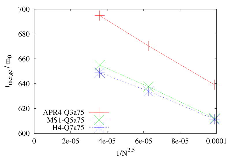
Figure 22: Merger time normalized by the total mass, $t_{\mathrm{merge}}/m_{0}$, vs grid resolutions for selected models. We assume a hypothetical convergence order 2.5 for all the models. Actual numerical data for APR4-Q3a75, MS1-Q5a75, and H4-Q7a75 show convergence orders 2.2, 2.9, and 3.1, respectively.

Finite grid resolutions are obvious sources of errors. First of all, we demonstrate that reasonable convergence behavior is observed in our numerical simulations. Figure 22 shows the merger time, $t_{\mathrm{merge}}$, as a function of grid resolutions represented by $N$ (see Sec. II.3 for the definition) for selected models. The exact convergence order estimated from numerical data varies among models and typically lies between 2 and 3. Taking the different accuracies for different parts of our code SACRA Yamamoto et al. (2008) into account, the observed behavior is reasonable.

Table 5: The same as Table 3 but for runs with different grid resolutions for selected models. The fiducial grid resolution adopted in the body text is $N=60$.

$N$	$M_{r>r_{\mathrm{AH}}}[M_{\odot}]$	$M_{\mathrm{bd}}[M_{\odot}]$	$M_{\mathrm{ej}}[M_{\odot}]$	$T_{\mathrm{ej}}$ ($\mathrm{e}\mathrm{r}\mathrm{g}$)	$P_{\mathrm{ej}}[M_{\odot}]$	$v_{\mathrm{ave}}$	$v_{\mathrm{ej}}$
APR4-Q3a75
60	0.194	0.182	0.0111	$5.48\text{\times}{10}^{50}$	$2.08\text{\times}{10}^{-3}$	0.235	0.187
48	0.210	0.201	0.0087	$3.98\text{\times}{10}^{50}$	$1.61\text{\times}{10}^{-3}$	0.227	0.186
40	0.206	0.198	0.0079	$3.40\text{\times}{10}^{50}$	$1.41\text{\times}{10}^{-3}$	0.219	0.178
APR4-Q5a75
60	0.068	0.059	0.0084	$4.77\text{\times}{10}^{50}$	$8.30\text{\times}{10}^{-4}$	0.252	0.099
48	0.070	0.063	0.0067	$3.60\text{\times}{10}^{50}$	$7.87\text{\times}{10}^{-4}$	0.246	0.118
40	0.074	0.069	0.0047	$2.43\text{\times}{10}^{50}$	$6.51\text{\times}{10}^{-4}$	0.239	0.137
MS1-Q5a75
60	0.356	0.277	0.0785	$5.55\text{\times}{10}^{51}$	$1.80\text{\times}{10}^{-2}$	0.281	0.223
48	0.361	0.282	0.0795	$5.26\text{\times}{10}^{51}$	$1.80\text{\times}{10}^{-2}$	0.272	0.226
40	0.370	0.290	0.0797	$5.28\text{\times}{10}^{51}$	$1.77\text{\times}{10}^{-2}$	0.272	0.222
H4-Q7a75
60	0.194	0.157	0.0375	$2.78\text{\times}{10}^{51}$	$7.19\text{\times}{10}^{-3}$	0.288	0.192
48	0.207	0.171	0.0360	$2.64\text{\times}{10}^{51}$	$6.89\text{\times}{10}^{-3}$	0.287	0.191
40	0.214	0.179	0.0341	$2.41\text{\times}{10}^{51}$	$6.64\text{\times}{10}^{-3}$	0.281	0.195

Table 5 compares characteristic quantities among different grid resolutions for selected models. It is evident that these quantities are not always monotonic with respect to the grid resolution. Such behavior is frequently seen in hydrodynamic quantities, which severely suffer low convergence order when shock waves exist. Relative errors are smaller for $M_{r>r_{\mathrm{AH}}}$ than for $M_{\mathrm{ej}}$, and this suggests that the accurate determination of boundaries separating bound and unbound material is an important but difficult task. If we assume the first-order convergence between $N=60$ and 48 results, the worst-case error with $N=60$ results are $\approx 30\%$, 40%, and 100% for $M_{r>r_{\mathrm{AH}}}$, $M_{\mathrm{bd}}$, and $M_{\mathrm{ej}}$, respectively. The accuracy of $M_{\mathrm{ej}}$ is especially low when the ejecta mass is as small as $M_{\mathrm{ej}}\lesssim 0.01M_{\odot}$, and the error decreases to $\lesssim 20\%$ for more massive ejecta. It is reasonable that the relative error is large for the small mass ejecta, where the absolute error is always estimated to be $\approx 0.005$–$0.01M_{\odot}$ for $M_{\mathrm{ej}}$.

A.2 Effect of an artificial atmosphere

An artificial atmosphere affects the ejecta properties. Some portion of the atmosphere happens to satisfy the unbound criterion, $u_{t}<-1$, as a result of hydrodynamic interaction, and this error spuriously increases the amount of the ejecta. At the same time, the atmosphere decelerates physical material ejected from neutron stars, and this error spuriously decreases the amount of ejecta. Low atmospheric density will mitigate both these errors. Another source of error is a steep density gradient at the neutron-star surface, which induces spurious shock heating in numerical simulations and helps the material to become unbound. Although this error will be suppressed as grid resolutions are improved to resolve the stellar surface accurately, lowering the atmospheric density at a fixed resolution does not always suppress it, because the shock could become strong.

Table 6: The same as Table 3 but with different values of $f_{\mathrm{at}}$ for APR4-Q3a75 with $N=60$ and 40. The fiducial value of $f_{\mathrm{at}}$ adopted in the body text is ${10}^{-12}$.

$f_{\mathrm{at}}$	$M_{r>r_{\mathrm{AH}}}[M_{\odot}]$	$M_{\mathrm{bd}}[M_{\odot}]$	$M_{\mathrm{ej}}[M_{\odot}]$	$T_{\mathrm{ej}}$ ($\mathrm{e}\mathrm{r}\mathrm{g}$)	$P_{\mathrm{ej}}[M_{\odot}]$	$v_{\mathrm{ave}}$	$v_{\mathrm{ej}}$
$N=60$
${10}^{-11}$	0.196	0.185	0.0111	$5.45\text{\times}{10}^{50}$	$2.07\text{\times}{10}^{-3}$	0.235	0.186
${10}^{-12}$	0.194	0.182	0.0111	$5.48\text{\times}{10}^{50}$	$2.08\text{\times}{10}^{-3}$	0.235	0.187
${10}^{-13}$	0.194	0.183	0.0112	$5.51\text{\times}{10}^{50}$	$2.08\text{\times}{10}^{-3}$	0.235	0.186
$N=40$
${10}^{-10}$	0.207	0.199	0.0080	$3.44\text{\times}{10}^{50}$	$1.43\text{\times}{10}^{-3}$	0.219	0.178
${10}^{-11}$	0.209	0.201	0.0078	$3.33\text{\times}{10}^{50}$	$1.38\text{\times}{10}^{-3}$	0.219	0.177
${10}^{-12}$	0.206	0.198	0.0079	$3.40\text{\times}{10}^{50}$	$1.41\text{\times}{10}^{-3}$	0.219	0.178

Table 6 compares characteristic quantities obtained with different values of $f_{\mathrm{at}}$. We find that ejecta quantities like $M_{\mathrm{ej}}$, $T_{\mathrm{ej}}$, and $P_{\mathrm{ej}}$ increase by $\approx 0.5\%$ for $N=60$ when the atmospheric density is decreased by an order of magnitude, while the corresponding change (either increase or decrease) is $\approx 1\%$–2% for $N=40$. Although the dominant mechanism responsible for the error is not certain, this suggests that the error associated with the artificial atmosphere will decrease significantly as grid resolutions are improved probably due to the suppression of spurious shocks at the stellar surface. We also find a similar amount of variations when we change the value of the atmospheric power-law index $n_{\mathrm{at}}$ from 3 to 2.

A.3 Effect of thermal correction $\Gamma_{\mathrm{th}}$

Dynamical mass ejection is expected to be governed basically by zero-temperature equations of state, because shock heating does not play a significant role. However, the ejecta properties depend weakly on the finite-temperature part of equations of state due to the spurious shock heating. Thus, the dependence of results on $\Gamma_{\mathrm{th}}$ also requires investigation.

Table 7: The same as Table 3 but for runs with different values of $\Gamma_{\mathrm{th}}$ for selected models. The fiducial value of $\Gamma_{\mathrm{th}}$ adopted in the body text is 1.8. All the simulations are performed with $N=60$.

$\Gamma_{\mathrm{th}}$	$M_{r>r_{\mathrm{AH}}}[M_{\odot}]$	$M_{\mathrm{bd}}[M_{\odot}]$	$M_{\mathrm{ej}}[M_{\odot}]$	$T_{\mathrm{ej}}$ ($\mathrm{e}\mathrm{r}\mathrm{g}$)	$P_{\mathrm{ej}}[M_{\odot}]$	$v_{\mathrm{ave}}$	$v_{\mathrm{ej}}$
APR4-Q3a75
1.6	0.196	0.184	0.0116	$5.95\text{\times}{10}^{50}$	$2.13\text{\times}{10}^{-3}$	0.240	0.184
1.8	0.194	0.182	0.0111	$5.48\text{\times}{10}^{50}$	$2.08\text{\times}{10}^{-3}$	0.235	0.187
2.0	0.192	0.184	0.0082	$3.69\text{\times}{10}^{50}$	$1.51\text{\times}{10}^{-3}$	0.225	0.184
H4-Q3a75
1.6	0.326	0.280	0.0455	$2.41\text{\times}{10}^{51}$	$9.34\text{\times}{10}^{-3}$	0.243	0.205
1.8	0.331	0.285	0.0454	$2.30\text{\times}{10}^{51}$	$9.22\text{\times}{10}^{-3}$	0.238	0.203
2.0	0.334	0.287	0.0464	$2.35\text{\times}{10}^{51}$	$9.28\text{\times}{10}^{-3}$	0.238	0.200
APR4-Q5a75
1.6	0.064	0.053	0.0108	$6.75\text{\times}{10}^{50}$	$8.82\text{\times}{10}^{-4}$	0.265	0.082
1.8	0.068	0.059	0.0084	$4.77\text{\times}{10}^{50}$	$8.30\text{\times}{10}^{-4}$	0.252	0.099
2.0	0.072	0.063	0.0089	$5.08\text{\times}{10}^{50}$	$9.80\text{\times}{10}^{-4}$	0.253	0.110
H4-Q5a75
1.6	0.314	0.261	0.0529	$3.74\text{\times}{10}^{51}$	$1.14\text{\times}{10}^{-2}$	0.281	0.216
1.8	0.316	0.266	0.0502	$3.33\text{\times}{10}^{51}$	$1.10\text{\times}{10}^{-2}$	0.272	0.220
2.0	0.320	0.269	0.0516	$3.34\text{\times}{10}^{51}$	$1.13\text{\times}{10}^{-2}$	0.269	0.220

Table 7 compares characteristic quantities obtained with different values of $\Gamma_{\mathrm{th}}$ for selected models. Results do not depend monotonically on the value of $\Gamma_{\mathrm{th}}$. This fact suggests that the effect of $\Gamma_{\mathrm{th}}$ is not very physical, and the difference is ascribed to numerical errors such as spurious shock heating. We checked that the differences develop during dynamical mass ejection which progresses over $\approx$2\text{\,}\mathrm{ms}$$ after the onset of merger, and late-time physical shock heating in the disk region does not introduce significant differences. The difference of results among different values of $\Gamma_{\mathrm{th}}$ is as large as $\approx 20\%$ when $M_{\mathrm{ej}}\lesssim 0.01M_{\odot}$ and tends to become small when the mass ejection is efficient. We regard the difference observed in Table 7 as an estimate of systematic uncertainty, which could converge as grid resolutions are improved.

A.4 Effect of different initial separations as a substitute for the eccentricity

Ejecta properties computed in our simulations deviate from those of hypothetical genuinely circular mergers due to unphysical eccentricities inherent in initial data. Specifically, different orbital and approaching velocities at the tidal disruption lead to deviations of characteristic quantities on the order of the eccentricity. Although this error can be eliminated by iterative eccentricity reduction Foucart et al. (2008); Kyutoku et al. (2014), it is demanding to reduce the eccentricities for all the models considered in this study.

Table 8: The same as Table 3 but with a different initial angular velocity, $m_{0}\Omega_{0}$, for APR4-Q3a75. The fiducial value of $m_{0}\Omega$ adopted in the body text is 0.036. All the simulations are performed with $N=60$.

$m_{0}\Omega_{0}$	$M_{r>r_{\mathrm{AH}}}[M_{\odot}]$	$M_{\mathrm{bd}}[M_{\odot}]$	$M_{\mathrm{ej}}[M_{\odot}]$	$T_{\mathrm{ej}}$ ($\mathrm{e}\mathrm{r}\mathrm{g}$)	$P_{\mathrm{ej}}[M_{\odot}]$	$v_{\mathrm{ave}}$	$v_{\mathrm{ej}}$
0.036	0.194	0.182	0.0111	$5.48\text{\times}{10}^{50}$	$2.08\text{\times}{10}^{-3}$	0.235	0.187
0.034	0.206	0.194	0.0112	$5.59\text{\times}{10}^{50}$	$2.11\text{\times}{10}^{-3}$	0.236	0.188
0.032	0.203	0.192	0.0109	$5.38\text{\times}{10}^{50}$	$2.02\text{\times}{10}^{-3}$	0.235	0.186
0.030	0.205	0.194	0.0114	$5.64\text{\times}{10}^{50}$	$2.12\text{\times}{10}^{-3}$	0.236	0.186

To estimate systematic errors associated with unphysical eccentricities, we instead compare results obtained by models with different values of $m_{0}\Omega_{0}$ with $e\sim 0.01$–0.02 for APR4-Q3a75. These models should merge at a different true anomaly (angle measured from the periapsis), admitting that it is very difficult to quantify this statement in numerical simulations. Therefore, the results will give us an idea of errors associated with eccentricities. As shown in Table 8, ejecta quantities like $M_{\mathrm{ej}}$, $T_{\mathrm{ej}}$, and $P_{\mathrm{ej}}$ fluctuate within $\pm 2.5\%$ as expected from the value of the eccentricity. Because the increase/decrease of a single ejecta quantity is accompanied by that of the others, derived quantities like $v_{\mathrm{ave}}$ and $v_{\mathrm{ej}}$ are relatively robust with respect to the unphysical eccentricity.

A.5 Comment on seemingly spurious high-velocity ejecta

In Sec. III.2.1, a small amount of unbound material is found to be ejected with a large velocity. We regard this component as an artifact, because the amount of high-velocity ejecta does not converge even approximately with respect to grid resolutions, admitting that ejecta cannot be decomposed unambiguously into physical and unphysical components unless reliable extrapolation to the continuum limit is performed. We speculate that this high-velocity ejecta is created by the artificial atmosphere and finite grid resolutions. They induce unphysical shocks at the stellar surface during the inspiral phase, and tenuous material continuously flows out from the inner edge of the neutron star. This artificial outflow is accumulated around the black hole and forms a small unphysical disk during the inspiral phase, whereas some of this disk may be supplied by the neutron star in a physical manner after the onset of mass shedding. A fraction of this unphysical disk is ejected impulsively during the merger (due possibly to the tidal torque exerted by the neutron star) with a large velocity reflecting the large escape velocity of black holes, i.e., the speed of light.

Appendix B Analytic estimate of ejecta opening angle

As we discussed in Sec. III.2.2, the ejecta geometry may be characterized by the opening angle in the meridional plane, $\varphi_{\mathrm{ej}}$, and that in the meridional plane, $\theta_{\mathrm{ej}}$. Before looking at numerical results, it is instructive to estimate these angles by analytic arguments for comparisons. These estimates help us to distinguish between expected and unexpected features.

Allowing more than one revolution, the opening angle of the dynamical ejecta in the equatorial plane should be given by

$$\varphi_{\mathrm{ej}}\approx 2\pi\frac{t_{\mathrm{td}}}{P_{\mathrm{td}}},$$ (70)

where $t_{\mathrm{td}}$ is the time scale of tidal disruption and $P_{\mathrm{td}}$ is the orbital period at the tidal disruption radius, $r_{\mathrm{td}}$ (see Eq. (36)). On one hand, $t_{\mathrm{td}}$ may be given approximately by the sound crossing time $t_{\mathrm{sc}}$ of the neutron star as

$$t_{\mathrm{td}}\approx t_{\mathrm{sc}}\propto\frac{1}{\sqrt{\bar{\rho}}}\;,$$ (71)

where $\bar{\rho}$ is the average stellar rest-mass density, which is determined by the equation of state. On the other hand, $P_{\mathrm{td}}$ should be given by

$$P_{\mathrm{td}}\approx 2\pi\sqrt{\frac{r_{\mathrm{td}}^{3}}{m_{0}}}\propto\sqrt{\frac{Q}{(1+Q)\bar{\rho}}}\;,$$ (72)

where Eq. (36) is used and spin-induced corrections are temporarily neglected. This suggests that the dependence of $\varphi_{\mathrm{ej}}$ on the equation of state is weak, because $\bar{\rho}$ cancels. This expression also suggests that $\varphi_{\mathrm{ej}}$ is smaller for a larger mass ratio, but the expected change is less than 10% between $Q=3$ and 7. Prograde black-hole spins will decrease $\varphi_{\mathrm{ej}}$, because the orbital frequency around a Kerr black hole is given by Bardeen et al. (1972)

$$\Omega_{\mathrm{K}}=\frac{\sqrt{M_{\mathrm{BH}}}}{r^{3/2}+\chi M_{\mathrm{BH}}^{3/2}},$$ (73)

and thus $P_{\mathrm{td}}$ increases as $\chi$ increases.

The opening angle of the dynamical ejecta in the meridional plane, $\theta_{\mathrm{ej}}$, is determined by the ratio of the velocity perpendicular to the orbital plane, $v_{\perp}$, to that in the equatorial direction, $v_{\parallel}$, as $\theta_{\mathrm{ej}}\approx\arctan(v_{\perp}/v_{\parallel})\approx v_{\perp}/v_{\parallel}$. This value should be given by the ratio of the neutron-star radius perpendicular to the orbital plane to the tidal disruption radius, $r_{\mathrm{td}}$ [see Eq. (36)]. Thus, the dependence of $\theta_{\mathrm{ej}}$ on the equation of state will be weak again, because both $v_{\parallel}$ and $v_{\perp}$ should scale linearly with $R_{\mathrm{NS}}$. Dependence on the mass ratio is expected to be $\theta_{\mathrm{ej}}\propto Q^{-1/3}$, inherited from $r_{\mathrm{td}}$, but the expected change is only 25% between $Q=3$ and 7. The spin will not modify the value of $\theta_{\mathrm{ej}}$.

References

- Harry and LIGO Scientific Collaboration (2010) G. M. Harry and LIGO Scientific Collaboration, Classical Quantum Gravity 27, 084006 (2010).
- F. Acernese et al. (2015) F. Acernese et al., Classical Quantum Gravity 32, 024001 (2015).
- Somiya (2012) K. Somiya, Classical Quantum Gravity 29, 124007 (2012).
- J. Abadie et al. (2010) J. Abadie et al., Class. Quant. Grav 27, 173001 (2010).
- Dominik et al. (2015) M. Dominik, E. Berti, R. O’Shaughnessy, I. Mandel, K. Belczynski, C. Fryer, D. Holz, T. Bulik, and F. Pannarale, Astrophys. J. 806, 263 (2015).
- Metzger and Berger (2012) B. D. Metzger and E. Berger, Astrophys. J. 746, 48 (2012).
- Piran et al. (2013) T. Piran, E. Nakar, and S. Rosswog, Mon. Not. R. Astron. Soc. 430, 2121 (2013).
- Nissanke et al. (2013) S. Nissanke, M. Kasliwal, and A. Georgieva, Astrophys. J. 767, 124 (2013).
- Messenger and Read (2012) C. Messenger and J. Read, Phys. Rev. Lett. 108, 091101 (2012).
- Schutz (1986) B. F. Schutz, Nature (London) 323, 310 (1986).
- Kochanek and Piran (1993) C. S. Kochanek and T. Piran, Astrophys. J. 417, L17 (1993).
- Nakar (2007) E. Nakar, Phys. Rep. 442, 166 (2007).
- Berger (2014) E. Berger, Annu. Rev. Astron. Astrophys. 52, 43 (2014).
- W. Fong et al. (2012) W. Fong et al., Astrophys. J. 756, 189 (2012).
- W. Fong et al. (2014) W. Fong et al., Astrophys. J. 780, 118 (2014).
- Ioka and Taniguchi (2000) K. Ioka and K. Taniguchi, Astrophys. J. 537, 327 (2000).
- McWilliams and Levin (2011) S. T. McWilliams and J. Levin, Astrophys. J. 742, 90 (2011).
- Tsang et al. (2012) D. Tsang, J. S. Read, T. Hinderer, A. L. Piro, and R. Bondarescu, Phys. Rev. Lett. 108, 011102 (2012).
- Paschalidis et al. (2013) V. Paschalidis, Z. B. Etienne, and S. L. Shapiro, Phys. Rev. D 88, 021504 (2013).
- Li and Paczyński (1998) L.-X. Li and B. Paczyński, Astrophys. J. 507, L59 (1998).
- (21) S. R. Kulkarni, arXiv:astro-ph/0510256 .
- Metzger et al. (2010a) B. D. Metzger, G. Martínez-Pinedo, S. Darbha, E. Quataert, A. Arcones, D. Kasen, R. Thomas, P. Nugent, I. V. Panov, and N. T. Zinner, Mon. Not. R. Astron. Soc. 406, 2650 (2010a).
- Kisaka et al. (2015) S. Kisaka, K. Ioka, and H. Takami, Astrophys. J. 802, 119 (2015).
- Nakar and Piran (2011) E. Nakar and T. Piran, Nature (London) 478, 82 (2011).
- Takami et al. (2014a) H. Takami, K. Kyutoku, and K. Ioka, Phys. Rev. D 89, 063006 (2014a).
- Lattimer and Schramm (1974) J. M. Lattimer and D. N. Schramm, Astrophys. J. 192, L145 (1974).
- Lattimer and Schramm (1976) J. M. Lattimer and D. N. Schramm, Astrophys. J. 210, 549 (1976).
- Shibata and Taniguchi (2011) M. Shibata and K. Taniguchi, Living Rev. Relativity 14, 6 (2011).
- Kyutoku et al. (2011a) K. Kyutoku, H. Okawa, M. Shibata, and K. Taniguchi, Phys. Rev. D 84, 064018 (2011a).
- Foucart et al. (2013a) F. Foucart, M. B. Deaton, M. D. Duez, L. E. Kidder, I. MacDonald, C. D. Ott, H. P. Pfeiffer, M. A. Scheel, B. Szilagyi, and S. A. Teukolsky, Phys. Rev. D 87, 084006 (2013a).
- Lovelace et al. (2013) G. Lovelace, M. D. Duez, F. Foucart, L. E. Kidder, H. P. Pfeiffer, M. A. Scheel, and B. Szilágyi, Classical Quantum Gravity 30, 135004 (2013).
- Deaton et al. (2013) M. B. Deaton, M. D. Duez, F. Foucart, E. O’Connor, C. D. Ott, L. E. Kidder, C. D. Muhlberger, M. A. Scheel, and B. Szilagyi, Astrophys. J. 776, 47 (2013).
- Foucart et al. (2014) F. Foucart, M. B. Deaton, M. Duez, E. O’Connor, C. D. Ott, R. Haas, L. E. Kidder, H. P. Pfeiffer, M. A. Scheel, and B. Szilagyi, Phys. Rev. D 90, 024026 (2014).
- Rosswog (2005) S. Rosswog, Astrophys. J. 634, 1202 (2005).
- Rosswog et al. (2013) S. Rosswog, T. Piran, and E. Nakar, Mon. Not. R. Astron. Soc. 430, 2585 (2013).
- Just et al. (2015) O. Just, A. Bauswein, R. A. Pulpillo, S. Goriely, and H.-T. Janka, Mon. Not. R. Astron. Soc. 448, 541 (2015).
- Lee and Kluźniak (1999) W. H. Lee and W. Kluźniak, Mon. Not. R. Astron. Soc. 308, 780 (1999).
- Lee (2000) W. H. Lee, Mon. Not. R. Astron. Soc. 318, 606 (2000).
- Lee (2001) W. H. Lee, Mon. Not. R. Astron. Soc. 328, 583 (2001).
- Faber et al. (2006a) J. A. Faber, T. W. Baumgarte, S. L. Shapiro, and K. Taniguchi, Astrophys. J. 641, L93 (2006a).
- Faber et al. (2006b) J. A. Faber, T. W. Baumgarte, S. L. Shapiro, K. Taniguchi, and F. A. Rasio, Phys. Rev. D 73, 024012 (2006b).
- Rantsiou et al. (2008) E. Rantsiou, S. Kobayashi, P. Laguna, and F. A. Rasio, Astrophys. J. 680, 1326 (2008).
- Ruffert and Janka (2010) M. Ruffert and H.-T. Janka, Astron. Astrophys. 514, A66 (2010).
- Hotokezaka et al. (2013a) K. Hotokezaka, K. Kiuchi, K. Kyutoku, H. Okawa, Y.-I. Sekiguchi, M. Shibata, and K. Taniguchi, Phys. Rev. D 87, 024001 (2013a).
- Bauswein et al. (2013) A. Bauswein, S. Goriely, and H.-T. Janka, Astrophys. J. 773, 78 (2013).
- Rosswog et al. (1999) S. Rosswog, M. Liebendörfer, F.-K. Thielemann, M. B. Davies, W. Benz, and T. Piran, Astron. Astrophys. 341, 499 (1999).
- Rosswog et al. (2000) S. Rosswog, M. B. Davies, F. Thielemann, and T. Piran, Astron. Astrophys. 360, 171 (2000).
- Yamamoto et al. (2008) T. Yamamoto, M. Shibata, and K. Taniguchi, Phys. Rev. D 78, 064054 (2008).
- Kyutoku et al. (2013) K. Kyutoku, K. Ioka, and M. Shibata, Phys. Rev. D 88, 041503 (2013).
- Shibata et al. (2009) M. Shibata, K. Kyutoku, T. Yamamoto, and K. Taniguchi, Phys. Rev. D 79, 044030 (2009).
- Shibata et al. (2012) M. Shibata, K. Kyutoku, T. Yamamoto, and K. Taniguchi, Phys. Rev. D 85, 127502(E) (2012).
- Kyutoku et al. (2010) K. Kyutoku, M. Shibata, and K. Taniguchi, Phys. Rev. D 82, 044049 (2010).
- Kyutoku et al. (2011b) K. Kyutoku, M. Shibata, and K. Taniguchi, Phys. Rev. D 84, 049902(E) (2011b).
- Read et al. (2009) J. S. Read, B. D. Lackey, B. J. Owen, and J. L. Friedman, Phys. Rev. D 79, 124032 (2009).
- Yakovlev and Pethick (2004) D. G. Yakovlev and C. J. Pethick, Annu. Rev. Astron. Astrophys. 42, 169 (2004).
- Akmal et al. (1998) A. Akmal, V. R. Pandharipande, and D. G. Ravenhall, Phys. Rev. C 58, 1804 (1998).
- Alford et al. (2005) M. Alford, M. Braby, M. Paris, and S. Reddy, Astrophys. J. 629, 969 (2005).
- Glendenning and Moszkowski (1991) N. K. Glendenning and S. A. Moszkowski, Phys. Rev. Lett. 67, 2414 (1991).
- Lackey et al. (2006) B. D. Lackey, M. Nayyar, and B. J. Owen, Phys. Rev. D 73, 024021 (2006).
- Müller and Serot (1996) H. Müller and B. D. Serot, Nucl. Phys. A 606, 508 (1996).
- Özel et al. (2012) F. Özel, D. Psaltis, R. Narayan, and A. S. Villarreal, Astrophys. J. 757, 55 (2012).
- Lattimer (2012) J. M. Lattimer, Ann. Rev. Nucl. Part. Sci. 62, 485 (2012).
- Hinderer (2008) T. Hinderer, Astrophys. J. 677, 1216 (2008).
- Hinderer (2009) T. Hinderer, Astrophys. J. 697, 964 (2009).
- Demorest et al. (2010) P. Demorest, T. Pennucci, S. Ransom, M. Roberts, and J. Hessels, Nature (London) 467, 1081 (2010).
- J. Antoniadis et al. (2013) J. Antoniadis et al., Science 340, 1233232 (2013).
- Kyutoku et al. (2009) K. Kyutoku, M. Shibata, and K. Taniguchi, Phys. Rev. D 79, 124018 (2009).
- (68) LORENE website, http://www.lorene.obspm.fr/.
- York (1979) J. W. York, in Gravitational Radiation, edited by L. Smarr (1979).
- York (1999) J. W. York, Phys. Rev. Lett. 82, 1350 (1999).
- Pfeiffer and York (2003) H. P. Pfeiffer and J. W. York, Phys. Rev. D 67, 044022 (2003).
- Brandt and Brügmann (1997) S. Brandt and B. Brügmann, Phys. Rev. Lett. 78, 3606 (1997).
- Bonazzola et al. (1997) S. Bonazzola, E. Gourgoulhon, and J.-A. Marck, Phys. Rev. D 56, 7740 (1997).
- Asada (1998) H. Asada, Phys. Rev. D 57, 7292 (1998).
- Teukolsky (1998) S. A. Teukolsky, Astrophys. J. 504, 442 (1998).
- Shibata (1998) M. Shibata, Phys. Rev. D 58, 024012 (1998).
- Kawaguchi et al. (2015) K. Kawaguchi, K. Kyutoku, H. Nakano, H. Okawa, M. Shibata, and K. Taniguchi, Phys. Rev. D 92, 024014 (2015).
- Shibata and Nakamura (1995) M. Shibata and T. Nakamura, Phys. Rev. D 52, 5428 (1995).
- Baumgarte and Shapiro (1998) T. W. Baumgarte and S. L. Shapiro, Phys. Rev. D 59, 024007 (1998).
- Campanelli et al. (2006) M. Campanelli, C. O. Lousto, P. Marronetti, and Y. Zlochower, Phys. Rev. Lett. 96, 111101 (2006).
- Baker et al. (2006) J. G. Baker, J. Centrella, D.-I. Choi, M. Koppitz, and J. van Meter, Phys. Rev. Lett. 96, 111102 (2006).
- Kurganov and Tadmor (2000) A. Kurganov and E. Tadmor, J. Comp. Phys. 160, 241 (2000).
- Colella and Woodward (1984) P. Colella and P. R. Woodward, J. Comp. Phys. 54, 174 (1984).
- Bauswein et al. (2010) A. Bauswein, H.-T. Janka, and R. Oechslin, Phys. Rev. D 82, 084043 (2010).
- Casares et al. (2014) J. Casares, I. Negueruela, M. Ribó, I. Ribas, J. M. Parades, A. Herrero, and S. Simón-Díaz, Nature (London) 505, 378 (2014).
- Özel et al. (2010) F. Özel, D. Psaltis, R. Narayan, and J. E. McClintock, Astrophys. J. 725, 1918 (2010).
- Kreidberg et al. (2012) L. Kreidberg, C. D. Bailyn, W. M. Farr, and V. Kalogera, Astrophys. J. 757, 36 (2012).
- McClintock et al. (2014) J. E. McClintock, R. Narayan, and J. F. Steiner, Space Sci. Rev. 183, 295 (2014).
- Foucart et al. (2013b) F. Foucart, L. Buchman, M. D. Duez, M. Grudich, L. E. Kidder, I. MacDonald, A. Mroue, H. P. Pfeiffer, M. A. Scheel, and B. Szilagyi, Phys. Rev. D 88, 064017 (2013b).
- Rosswog (2007) S. Rosswog, Mon. Not. R. Astron. Soc. 376, L48 (2007).
- Rossi and Begelman (2009) E. M. Rossi and M. C. Begelman, Mon. Not. R. Astron. Soc. 392, 1451 (2009).
- Kyutoku et al. (2014) K. Kyutoku, M. Shibata, and K. Taniguchi, Phys. Rev. D 90, 064006 (2014).
- Lousto et al. (2010) C. O. Lousto, H. Nakano, Y. Zlochower, and M. Campanelli, Phys. Rev. D 82, 104057 (2010).
- Ruiz et al. (2008) M. Ruiz, M. Alcubierre, D. Núñez, and R. Takahashi, Gen. Rel. Grav. 40, 1705 (2008).
- Reisswig and Pollney (2011) C. Reisswig and D. Pollney, Classical Quantum Gravity 28, 195015 (2011).
- Wiggins and Lai (2000) P. Wiggins and D. Lai, Astrophys. J. 532, 530 (2000).
- Ferrari et al. (2009) V. Ferrari, L. Gualtieri, and F. Pannarale, Classical Quantum Gravity 26, 125004 (2009).
- Bardeen et al. (1972) J. M. Bardeen, W. H. Press, and S. A. Teukolsky, Astrophys. J. 178, 347 (1972).
- Chamel and Haensel (2008) N. Chamel and P. Haensel, Living Rev. Relativity 11, 10 (2008).
- Wanajo et al. (2014) S. Wanajo, Y. Sekiguchi, N. Nishimura, K. Kiuchi, K. Kyutoku, and M. Shibata, Astrophys. J. 789, L39 (2014).
- Bauswein et al. (2014) A. Bauswein, R. A. Pulpillo, H. Janka, and S. Goriely, Astrophys. J. 795, L9 (2014).
- Sekiguchi et al. (2015) Y. Sekiguchi, K. Kiuchi, K. Kyutoku, and M. Shibata, Phys. Rev. D 91, 064059 (2015).
- Rosswog et al. (2014) S. Rosswog, O. Korobkin, A. Arcones, F.-K. Thielemann, and T. Piran, Mon. Not. R. Astron. Soc. 439, 744 (2014).
- (104) K. Kiuchi, Y. Sekiguchi, K. Kyutoku, M. Shibata, K. Taniguchi, and T. Wada, arXiv:1506.06811 .
- (105) Y. Sekiguchi et al., (unpublished) .
- Lee et al. (2009) W. H. Lee, E. Ramirez-Ruiz, and D. López-Cámara, Astrophys. J. 699, L93 (2009).
- Fernández and Metzger (2013) R. Fernández and B. D. Metzger, Mon. Not. R. Astron. Soc. 435, 502 (2013).
- Laguna et al. (1993) P. Laguna, W. A. Miller, W. H. Zurek, and M. B. Davies, Astrophys. J. 410, L83 (1993).
- Cutler et al. (1994) C. Cutler, D. Kennefick, and E. Poisson, Phys. Rev. D 50, 3816 (1994).
- Glampedakis and Kennefick (2002) K. Glampedakis and D. Kennefick, Phys. Rev. D 66, 044002 (2002).
- Foucart (2012) F. Foucart, Phys. Rev. D 86, 124007 (2012).
- Hotokezaka et al. (2013b) K. Hotokezaka, K. Kyutoku, M. Tanaka, K. Kiuchi, Y. Sekiguchi, M. Shiata, and S. Wanajo, Astrophys. J. 778, L16 (2013b).
- Lacy et al. (1982) J. H. Lacy, C. H. Townes, and D. J. Hollenbach, Astrophys. J. 262, 120 (1982).
- Mészáros and Rees (2000) P. Mészáros and M. J. Rees, Astrophys. J. 530, 292 (2000).
- Nagakura et al. (2014) H. Nagakura, K. Hotokezaka, Y. Sekiguchi, M. Shibata, and K. Ioka, Astrophys. J. 784, L28 (2014).
- Rees (1988) M. J. Rees, Nature (London) 333, 523 (1988).
- Phinney (1989) E. S. Phinney, in The center of the Galaxy, IAU Symposium, edited by M. Morris (1989) p. 543.
- Chawla et al. (2010) S. Chawla, M. Anderson, M. Besselman, L. Lehner, S. L. Liebling, P. M. Motl, and D. Neilsen, Phys. Rev. Lett. 105, 111101 (2010).
- Metzger et al. (2010b) B. D. Metzger, A. Arcones, E. Quataert, and G. Martínez-Pinedo, Mon. Not. R. Astron. Soc. 402, 2771 (2010b).
- Evans and Kochanek (1989) C. R. Evans and C. S. Kochanek, Astrophys. J. 346, L13 (1989).
- Lodato et al. (2009) G. Lodato, A. R. King, and J. E. Pringle, Mon. Not. R. Astron. Soc. 392, 332 (2009).
- Fitchett (1983) M. J. Fitchett, Mon. Not. R. Astron. Soc. 203, 1049 (1983).
- Lackey et al. (2012) B. D. Lackey, K. Kyutoku, M. Shibata, P. R. Brady, and J. L. Friedman, Phys. Rev. D 85, 044061 (2012).
- Pannarale et al. (2013) F. Pannarale, E. Berti, K. Kyutoku, and M. Shibata, Phys. Rev. D 88, 084011 (2013).
- Lackey et al. (2014) B. D. Lackey, K. Kyutoku, M. Shibata, P. R. Brady, and J. L. Friedman, Phys. Rev. D 89, 043009 (2014).
- Wiseman (1992) A. G. Wiseman, Phys. Rev. D 46, 1517 (1992).
- Blanchet et al. (2005) L. Blanchet, M. S. S. Qusailah, and C. M. Will, Astrophys. J. 635, 508 (2005).
- Read et al. (2013) J. S. Read, L. Baiotti, J. D. E. Creighton, J. L. Friedman, B. Giacomazzo, K. Kyutoku, C. Markakis, L. Rezzolla, M. Shibata, and K. Taniguchi, Phys. Rev. D 88, 044042 (2013).
- Bernuzzi et al. (2014) S. Bernuzzi, A. Nagar, S. Balmelli, T. Dietrich, and M. Ujevic, Phys. Rev. Lett. 112, 201101 (2014).
- Damour and Nagar (2010) T. Damour and A. Nagar, Phys. Rev. D 81, 084016 (2010).
- Vines et al. (2011) J. Vines, É. É. Flanagan, and T. Hinderer, Phys. Rev. D 83, 084051 (2011).
- Kidder et al. (1993) L. E. Kidder, C. M. Will, and A. G. Wiseman, Phys. Rev. D 47, R4183 (1993).
- Damour (2001) T. Damour, Phys. Rev. D 64, 124013 (2001).
- Vallisneri (2000) M. Vallisneri, Phys. Rev. Lett. 84, 3519 (2000).
- Tanaka et al. (2014) M. Tanaka, K. Hotokezaka, K. Kyutoku, S. Wanajo, K. Kiuchi, Y. Sekiguchi, and M. Shibata, Astrophys. J. 780, 31 (2014).
- Kasen et al. (2013) D. Kasen, N. R. Badnell, and J. Barnes, Astrophys. J. 774, 25 (2013).
- Tanaka and Hotokezaka (2013) M. Tanaka and K. Hotokezaka, Astrophys. J. 775, 113 (2013).
- Takami et al. (2014b) H. Takami, T. Nozawa, and K. Ioka, Astrophys. J. 789, L6 (2014b).
- Roberts et al. (2011) L. F. Roberts, D. Kasen, W. H. Lee, and E. Ramirez-Ruiz, Astrophys. J. 736, L21 (2011).
- Grossman et al. (2014) D. Grossman, O. Kolobkin, S. Rosswog, and T. Piran, Mon. Not. R. Astron. Soc. 439, 757 (2014).
- Höflich (1991) P. Höflich, Astron. Astrophys. 246, 481 (1991).
- Jeffery (1989) D. J. Jeffery, Astrophys. J. Suppl. 71, 951 (1989).
- Ioka and Mészáros (2005) K. Ioka and P. Mészáros, Astrophys. J. 619, 684 (2005).
- Chevalier and Fransson (2006) R. A. Chevalier and C. Fransson, Astrophys. J. 651, 381 (2006).
- Taylor et al. (2004) G. B. Taylor, D. A. Frail, E. Berger, and S. R. Kulkarni, Astrophys. J. 609, L1 (2004).
- Foucart et al. (2008) F. Foucart, L. E. Kidder, H. P. Pfeiffer, and S. A. Teukolsky, Phys. Rev. D 77, 124051 (2008).