Modeling magnetized neutron stars using resistive MHD

Abstract

This work presents an implementation of the resistive MHD equations for a generic algebraic Ohm’s law which includes the effects of finite resistivity within full General Relativity. The implementation naturally accounts for magnetic-field-induced anisotropies and, by adopting a phenomenological current, is able to accurately describe electromagnetic fields in the star and in its magnetosphere. We illustrate the application of this approach in interesting systems with astrophysical implications; the aligned rotator solution and the collapse of a magnetized rotating neutron star to a black hole.

1 Introduction

Magnetic fields play an important role in the dynamics of many relativistic astrophysical systems such as pulsars, magnetars, gamma-ray burst (GRBs) and active galactic nuclei (AGNs). In many of these scenarios, the Ohmic diffusion timescales of the magnetized plasma is much longer than the characteristic dynamical timescale of the system, so one can formally take the limit of infinite electrical conductivity. This is regarded as the ideal MHD limit, and it is in general a good approximation to describe astrophysical plasmas. Furthermore, such a limit is described by a relatively manageable, but certainly involved hyperbolic system of equations without stiff terms which facilitates its computational implementation. The ideal MHD limit has been extensively used in the last years to study many of the previous systems (i.e., which basically consist of magnetized neutron stars and black hole accretion disks) in the fully non-linear regime.

In spite of its success and convenience, the ideal MHD approximation also has some limitations. At a purely theoretical level, the assumption of vanishing electrical resistivity prevents some important physical phenomena such as dissipation and reconnection of the magnetic field lines. Reconnection efficiently converts magnetic energy into heat and kinetical energy in very short timescales. This process is believed to be the mechanism originating many energetic emissions, such as in soft gamma-ray repeaters (which could be explained by giant magnetar flares), the Y-point of pulsar magnestosphere or even the short Gamma-Ray Bursts (Uzdensky, 2011). In order to describe such processes, schemes going beyond the ideal MHD limit are required.

At the numerical level, all numerical schemes inherit some numerical resistivity which depends strongly on the resolution, making difficult to disentangle physical phenomena from numerical artifacts especially in highly demanding computational scenarios. The presence of magnetic fields demands relatively high resolution to accurately capture all the physical processes involved, many of them occurring at very small scales. This high resolution is particularly important in the case of instabilities which amplify the magnetic field, such as the Kelvin-Helmholtz instability occurring during the merger of binary neutron stars (Price & Rosswog, 2006; Obergaulinger et al., 2010), and the Magneto-Rotational Instability (MRI) occurring in accretion disks (Balbus & Hawley, 1991; Hawley & Balbus, 1991; Hawley et al., 1995; Balbus & Hawley, 1998). Accurate modeling of the rarefied magnetospheres of compact objects similarly requires high resolution. The electromagnetic fields in this region may be easier to model by adopting a different limit of the MHD equations known as the force-free limit (Goldreich & Julian, 1969). In this approximation the fluid inertia is neglected, implying that the fluid does not influence directly the dynamics of the electromagnetic fields.

One possibility to overcome these limitations is to consider instead the resistive MHD framework and solve the full Maxwell and hydrodynamic equations. The coupling between these two is provided by the current –by a suitable Ohm’s law–. With a convenient choice of current, including both induction and Ohmic terms, it is possible to recover both the ideal MHD limit, as well as the finite-resistivity scheme required to describe physical dissipation and reconnections. The effect of small-scales-dynamics can also be modeled with moderate resolutions by using a suitable current. Finally, magnetically dominated magnetospheres can be described by a phenomenological current that decouples the fluid from the force-free EM fields.

The numerical evolution of this resistive MHD code is not free of difficulties. The resistive MHD equations can be regarded as an hyperbolic system with relaxation terms that become stiff for some limits of the current. Consequently, numerical evolution of this system represents a numerical challenge, and several works have recently explored different possibilities to implement it (Komissarov, 2007; Palenzuela et al., 2009; Dumbser & Zanotti, 2009; Zenitani et al., 2010; Takamoto & Inoue, 2011; Bucciantini & Del Zanna, 2012; Dionysopoulou et al., 2012). In this work we take a step further in the development of one of these approaches, based on the Implicit-Explicit (IMEX) Runge-Kutta. Our aim is to model both the interior and the exterior of a star with a phenomenological current based on physical arguments. This will be particularly interesting to study the electromagnetic emissions of astrophysical relativistic systems involving magnetized neutron stars.

The capabilities of our approach are tested by considering the force-free aligned rotator solution, a well studied problem in the context of pulsar magnetospheres  (Contopoulos & Spitkovsky, 2006; Spitkovsky, 2006; McKinney, 2006; Bucciantini et al., 2006; Kalapotharakos & Contopoulos, 2009; Li et al., 2012; Tchekhovskoy & Spitkovsky, 2012). These works were restricted to flat spacetime and excluded the interior of the star from the computational domain, thus side-stepped the stiffness problem mentioned above. Recently a hybrid approach, matching both the ideal and force-free system of equations, revisited this problem within a framework capable of studying both star and surrounding magnetosphere within General Relativity (Lehner et al., 2011). However such a scheme still relies on two different approximations applied in two regions. The approach we present here finally allows for treating the system from a global point of view with a single, general relativistic, framework.

We also revisit another important astrophysical scenario with a much less understood dynamics; the collapse of a magnetized neutron star to a black hole. This system represents even a more challenging problem because of the strong gravity fields, and it has been studied numerically by considering different approximations. An early study matched an analytical solution for the star to an electrovacuum magnetosphere (Baumgarte & Shapiro, 2003). More recently, further realism was achieved by adopting the hybrid scheme that matched the numerical solution of the star to force-free magnetosphere (Lehner et al., 2011). A step towards studying this system within a common, resistive, framework was presented in (Dionysopoulou et al., 2012), although the star’s exterior was treated as an electrovacuum magnetosphere. Our approach presented here is able to consistently study the star and its force-free magnetosphere within the general relativistic resistive MHD equations.

The paper is organized as follows. Section 2 summarizes the fully relativistic resistive MHD system, which is slightly different from the one adopted in (Dionysopoulou et al., 2012). In Section 3 it is discussed a generic family of algebraic Ohm’s law, and how to construct a phenomenological current to recover both the ideal MHD and the force-free limits. Section 4 summarizes briefly the IMEX Runge-Kutta methods and different techniques to solve generically the implicit step for any algebraic form of the relaxation terms. The application of these methods to the resistive MHD system is performed is section 5. Section 6 presents our numerical results for the aligned rotator and the collapse of a neutron star to a black hole. We conclude with some remarks.

Throughout this work we adopt geometric units such that $G=c=1$, and the convention where greek indices $\mu,\nu,\alpha,...$ denote spacetime components (ie, from $0$ to $3$), while roman indices $i,j,k,...$ denote spatial ones. Bold letters will represent vectors.

2 The evolution equations

This section summarizes the general relativistic resistive magnetohydrodynamic equations, that will allow us to model self-gravitating magnetized fluids. The evolution of the spacetime geometry is governed by Einstein equations. The electromagnetic fields and the fluid obey, respectively, the Maxwell and the General Relativistic Hydrodynamic equations. The closure of the system is given by two constitutive equations; the first one is the equation of state, which relates the pressure to the other fluid variables. The second one is Ohm’s law, –defining the coupling between the fluid and the electromagnetic fields– which will be described in the next section.

2.1 Einstein Equations

The geometry of the spacetime can be obtained by solving the four-dimensional Einstein equations. These equations can be recast as a standard initial value problem by splitting explicitly the time and the space coordinates through a 3+1 decomposition, such that the line element can be expressed as

$$ds^{2} = g_{\mu\nu}\,dx^{\mu}dx^{\nu}$$ (1)

$$= -\alpha^{2}\,dt^{2}+\gamma_{ij}\left(dx^{i}+\beta^{i}\,dt\right)\left(dx^{j}+\beta^{j}\,dt\right),$$

where $g_{\mu\nu}$ is the spacetime metric, $\gamma_{ij}=g_{ij}$ is the intrinsic metric of the spacelike hypersurfaces, and the lapse function $\alpha$ and the shift vector $\beta^{i}$ relates how the coordinates change between neighboring hypersurfaces. The normal to the hypersurfaces is given explicitly by

$$n^{\mu}=\frac{1}{\alpha}(1,-\beta^{i})~{}~{}~{},~{}~{}~{}n_{\mu}=(-\alpha,0)~{}~{}.$$ (2)

Indices on spacetime quantities are raised and lowered with the 4-metric and its inverse, while the 3-metric and its inverse are used to raise and lower indices on spatial quantities.

The rate of change of the intrinsic curvature from one hypersurface to another is given by the extrinsic curvature

$$K_{ij}=-\frac{1}{2\alpha}(\partial_{t}-{\cal L}_{\beta})\gamma_{ij}$$ (3)

where ${\cal L}_{\beta}$ is the Lie derivative along the vector $\beta^{i}$.

At any given time, the spacetime geometry is then fully defined by the $3+1$ variables $\{\alpha,\beta^{i},\gamma_{ij},K_{ij}\}$. We adopt the Baumgarte-Shapiro-Shibata-Nakamura (BSSN) formulation of Einstein’s equations to evolve a suitable combination of these fields, in a form very close to the presented in (Campanelli et al., 2006).

2.2 Maxwell equations

The electromagnetic fields follow Maxwell equations, that in their extended version can be written as (Palenzuela et al., 2010c)

$$\nabla_{\mu}(F^{\mu\nu}+g^{\mu\nu}\psi) = -I^{\nu}+\kappa n^{\nu}\psi$$ (4)

$$\nabla_{\mu}({}^{*}F^{\mu\nu}+g^{\mu\nu}\phi) = \kappa n^{\nu}\phi~{},$$ (5)

where $\{F^{\mu\nu},^{*}F^{\mu\nu}\}$ are the Maxwell and the Faraday tensors, $I^{\nu}$ is the electric current and $\{\phi,\psi\}$ are scalars introduced to control dynamically the constraints by exponentially damping them in a characteristic time $1/\kappa$ (Dedner et al., 2002). When both the electric and magnetic susceptibility of the medium vanish, like in vacuum or in a highly ionized plasma, the Faraday tensor is simply the dual of the Maxwell one,

$${}^{*}F^{\mu\nu}=\frac{1}{2}\,\epsilon^{\mu\nu\alpha\beta}\,F_{\alpha\beta}~{},\qquad F^{\mu\nu}=-\frac{1}{2}\,\epsilon^{\mu\nu\alpha\beta}~{}{}^{*}F_{\alpha\beta}$$ (6)

where $\epsilon^{\mu\nu\alpha\beta}$ is the Levi-Civita pseudotensor of the spacetime, related to the 4-indices Levi-Civita symbol $\eta^{\mu\nu\alpha\beta}$ by

$$\epsilon^{\mu\nu\alpha\beta}=\frac{1}{\sqrt{g}}~{}\eta^{\mu\nu\alpha\beta}\qquad\epsilon_{\mu\nu\alpha\beta}=-\sqrt{g}~{}\eta_{\mu\nu\alpha\beta}~{}.$$ (7)

In this case, both tensors can be decomposed in terms of the electric and magnetic fields,

$$F^{\mu\nu} = n^{\mu}E^{\nu}-n^{\nu}E^{\mu}+\epsilon^{\mu\nu\alpha\beta}~{}B_{\alpha}~{}n_{\beta}$$ (8)

$${}^{*}F^{\mu\nu} = n^{\mu}B^{\nu}-n^{\nu}B^{\mu}-\epsilon^{\mu\nu\alpha\beta}~{}E_{\alpha}~{}n_{\beta}$$ (9)

such that $E^{\mu}$ and $B^{\mu}$ are the electric and magnetic fields measured by a normal observer $n^{\mu}$. Both fields are purely spatial, that is, $E^{\mu}n_{\mu}=B^{\mu}n_{\mu}=0$.

The covariant Maxwell equations (4, 5) can be written, by performing the 3+1 decomposition, in term of the electromagnetic fields and the divergence-cleaning scalars (Palenzuela et al., 2010c) as,

$$(\partial_{t}-{\cal L}_{\beta})E^{i} - \epsilon^{ijk}\nabla_{j}(\alpha B_{k})+\alpha\gamma^{ij}\nabla_{j}\psi$$

$$= \alpha trKE^{i}-\alpha J^{i}$$

$$(\partial_{t}-{\cal L}_{\beta})\psi + \alpha\nabla_{i}E^{i}=\alpha q-\alpha\kappa\psi$$ (11)

$$(\partial_{t}-{\cal L}_{\beta})B^{i} + \epsilon^{ijk}\nabla_{j}(\alpha E_{k})+\alpha\gamma^{ij}\nabla_{j}\phi$$

$$= \alpha trKB^{i}$$

$$(\partial_{t}-{\cal L}_{\beta})\phi + \alpha\nabla_{i}B^{i}=-\alpha\kappa\phi~{}~{}.$$ (13)

where $\epsilon^{ijk}\equiv\epsilon^{ijk\alpha}n_{\alpha}=\eta^{ijk}/\sqrt{\gamma}$ is the three-dimensional Levi-Civita pseudotensor. Since $F^{\mu\nu}$ is antisymmetric, the four-divergence of equation (4) leads to an additional equation for the current conservation of Maxwell solutions,

$$\nabla_{\mu}I^{\,\mu}=0~{}.$$ (14)

The electric current $I^{\nu}$ can be decomposed into components along and perpendicular to the vector $n^{\nu}$,

$$I^{\nu}=n^{\nu}q+J^{\nu}~{}~{},$$ (15)

where $q$ and $J^{\nu}$ are the charge density and the current as observed by a normal observer $n^{\nu}$. Again, $J^{\nu}$ is purely spatial, so $J^{\nu}n_{\nu}=0$. The current conservation (14) can be expressed, with the 3+1 decomposition, as

$$(\partial_{t}-{\cal L}_{\beta})q+\nabla_{i}(\alpha J^{i})=\alpha trKq$$ (16)

Only a prescription for the spatial components $J^{i}$, which will determine the coupling between the EM fields and the fluid, is required to complete the system of Maxwell equations. This relation, commonly known as Ohm’s law, will be discussed in detail in section 3.

2.3 Hydrodynamic equations

A perfect fluid minimally coupled to an electromagnetic field is described by the total stress-energy tensor

$$T_{\mu\nu} = \left[\rho(1+\epsilon)+p\right]u_{\mu}u_{\nu}+pg_{\mu\nu}$$ (17)

$$+ {F_{\mu}}^{\lambda}F_{\nu\lambda}-\frac{1}{4}g_{\mu\nu}~{}F^{\lambda\alpha}F_{\lambda\alpha}$$

where a factor $1/\sqrt{4\pi}$ has been absorbed in the definition of the electromagnetic fields. Here $\rho$ is the rest mass density, $\epsilon$ the internal energy and $p$ is the pressure, given by a closure relation $p=p(\rho,\epsilon)$ commonly known as the equation of state (EoS). These fluid quantities are measured in the rest frame of the fluid element. However, to describe the system is usually more convenient to adopt an Eulerian perspective where coordinates are not tied to the flow of the fluid. The four-velocity $u^{\mu}$ describes how the fluid moves with respect to the Eulerian observers, and can be decomposed into space and time components,

$$u^{\mu}=W\left(n^{\mu}+v^{\mu}\right)$$ (18)

where $v^{\mu}$ corresponds to the familiar three-dimensional velocities as measured by Eulerian observers (i.e., $v^{\mu}n_{\mu}=0$). The time component is defined by the normalization relation $u^{\mu}u_{\mu}=-1$, such that

$$W=-n_{\mu}u^{\mu}=(1-v_{i}v^{i})^{-1/2}~{},~{}~{}$$ (19)

where we can now recognize $W$ as the Lorentz factor.

In summary, the magnetized fluid is described by the physical fields (i.e., the fluid variables and the electromagnetic fields) plus the divergence cleaning scalars, which form the set of primitive variables $(\rho,\epsilon,p,v^{i},E^{i},B^{i},q,\phi,\psi)$ The matter evolution must comply with the conservation of the total stress-energy tensor

$$\nabla_{\nu}T^{\mu\nu}=0,$$ (20)

which can be expressed as a system of conservation laws for the energy density $U$ and the momentum density $S_{i}$, defined from the projections of the stress-energy tensor

$$U=n_{\mu}n_{\nu}T^{\mu\nu}~{}~{},~{}~{}S_{i}=-n^{\mu}T_{\mu i}~{}~{},~{}~{}S_{ij}=T_{ij}~{}~{}.$$ (21)

In addition to the conservation of energy and momentum, the fluid usually also conserves the total number of particles,

$$\nabla_{\mu}(\rho u^{\mu})=0$$ (22)

where $\rho u^{\mu}$ is the baryon number density. This equation is just the relativistic generalization of the conservation of mass.

As mentioned above, it is necessary to specify the EOS to define the pressure and complete the system of hydrodynamic equations. Along this paper we will consider either the polytropic EoS $p=K\rho^{\Gamma}$, which is a good approximation to describe cold stars, and the ideal gas EoS $p=(\Gamma-1)\rho\epsilon$, which allows for shock heating in the fluid.

2.4 Resistive MHD system

The evolution of the electromagnetic fields follows the Maxwell equations and the conservation of charge, while the fluid fields are governed by the conservation of the total energy, momentum and baryonic number. In order to capture accurately the weak solutions of these non-linear equations in presence of shocks it is important to express them as a set of local conservation laws, namely

$$\partial_{t}(\sqrt{\gamma}B^{i}) + \partial_{k}[\sqrt{\gamma}\left(-\beta^{k}B^{i}+\alpha(\epsilon^{ikj}E_{j}+\gamma^{ik}\phi)\right)]$$

$$= -\sqrt{\gamma}B^{k}(\partial_{k}\beta^{i})+\sqrt{\gamma}\phi\left(\gamma^{ij}\partial_{j}\alpha-\alpha\gamma^{jk}\Gamma^{i}_{jk}\right)$$

$$\partial_{t}(\sqrt{\gamma}E^{i}) + \partial_{k}[\sqrt{\gamma}\left(-\beta^{k}E^{i}-\alpha(\epsilon^{ikj}B_{j}-\gamma^{ik}\psi)\right)]$$

$$= -\sqrt{\gamma}E^{k}(\partial_{k}\beta^{i})+\sqrt{\gamma}\psi\left(\gamma^{ij}\partial_{j}\alpha-\alpha\gamma^{jk}\Gamma^{i}_{jk}\right)$$

$$-\alpha\sqrt{\gamma}J^{i}$$

$$\partial_{t}(\sqrt{\gamma}\phi) + \partial_{k}[\sqrt{\gamma}(-\beta^{k}\phi+\alpha B^{k})]$$

$$= \sqrt{\gamma}[-\alpha\,\phi\,trK+B^{k}(\partial_{k}\alpha)-\alpha\kappa\phi]$$

$$\partial_{t}(\sqrt{\gamma}\psi) + \partial_{k}[\sqrt{\gamma}(-\beta^{k}\psi+\alpha E^{k})]$$

$$= \sqrt{\gamma}[-\alpha\,\psi\,trK+E^{k}(\partial_{k}\alpha)+\alpha q-\alpha\kappa\psi]$$

$$\partial_{t}(\sqrt{\gamma}q) + \partial_{k}[\sqrt{\gamma}(-\beta^{k}q+\alpha J^{k})]=0$$ (27)

$$\partial_{t}(\sqrt{\gamma}D) + \partial_{k}[\sqrt{\gamma}(-\beta^{k}+\alpha v^{k})D]=0$$ (28)

$$\partial_{t}(\sqrt{\gamma}\tau) + \partial_{k}[\sqrt{\gamma}\left(-\beta^{k}\tau+\alpha(S^{k}-v^{k}D)\right)]$$ (29)

$$= \sqrt{\gamma}[\alpha S^{ij}K_{ij}-S^{j}\partial_{j}\alpha]$$ (30)

$$\partial_{t}(\sqrt{\gamma}S_{i}) + \partial_{k}[\sqrt{\gamma}(-\beta^{k}S_{i}+\alpha{S^{k}}_{i})]$$

$$= \sqrt{\gamma}[\frac{\alpha}{2}S^{jk}{\partial_{i}}\gamma_{jk}+S_{j}\partial_{i}\beta^{j}-(\tau+D)\partial_{i}\alpha]$$

where we have defined

$$D = \rho W~{},~{}~{}~{}$$ (32)

$$\tau = hW^{2}-p+\frac{1}{2}(E^{2}+B^{2})-\rho W~{},~{}~{}~{}$$ (33)

$$S_{i} = hW^{2}v_{i}+\epsilon_{ijk}E^{j}B^{k}~{},~{}~{}~{}$$ (34)

$$S_{ij} = hW^{2}v_{i}v_{j}+\gamma_{ij}p$$

$$-E_{i}E_{j}-B_{i}B_{j}+\frac{1}{2}\gamma_{ij}(E^{2}+B^{2})~{},~{}~{}$$

and the enthalpy $h\equiv\rho(1+\epsilon)+p$. This form of the relativistic resistive MHD equations is basically the same presented already in (Dionysopoulou et al., 2012). Another similar formulation has also been derived recently (Bucciantini & Del Zanna, 2012). Notice also that the energy conservation has been expressed in terms of the quantity $\tau\equiv U-D$ to recover the Newtonian limit of the energy density.

3 Coupling between the EM fields and the fluid

Maxwell and hydrodynamic equations are coupled by means of the current ${I}^{\mu}$, whose explicit form generically depends on the electromagnetic fields and the local fluid properties measured in the comoving frame. Consequently, it is convenient to introduce the electric and magnetic fields measured by an observer comoving with the fluid, namely $e^{\mu}\equiv F^{\mu\nu}u_{\nu}$ and $b^{\mu}\equiv{}^{*}F^{\mu\nu}u_{\nu}$. Notice that, since $e^{\mu}u_{\mu}=b^{\mu}u_{\mu}=0$, there are only three independent components. The Maxwell and Faraday tensors can therefore be expressed as

$$F^{\mu\nu} = u^{\mu}e^{\nu}-u^{\nu}e^{\mu}+\epsilon^{\mu\nu\alpha\beta}~{}b_{\alpha}~{}u_{\beta}$$ (36)

$${}^{*}F^{\mu\nu} = u^{\mu}b^{\nu}-u^{\nu}b^{\mu}-\epsilon^{\mu\nu\alpha\beta}~{}e_{\alpha}~{}u_{\beta}$$ (37)

and the electric current can be decomposed into components along and transverse to $u^{\nu}$,

$$I^{\mu}=u^{\mu}\tilde{q}+j^{\mu}~{}~{},$$ (38)

where $j^{\mu}u_{\mu}=0$ and $\tilde{q}$ is the charge density measured by the comoving observer. The relation with the Eulerian quantities (15) can be obtained from

$$q=-n_{\mu}I^{\mu}=W\tilde{q}-n_{\mu}j^{\mu}~{}~{}.$$ (39)

Substituting these results into eq. (38) and using the 3+1 decomposition of the four-velocity, one can write the spatial components of the current as

$$I_{i}=J_{i}=(q+j^{\mu}n_{\mu})v_{i}+j_{i}~{}~{}.$$ (40)

Since the charge density follows directly from the current conservation (16), the prescription for the three-dimensional electrical current $J_{i}$ is the only missing piece to completely determine Maxwell equations.

3.1 Generalized covariant Ohm’s law

A standard prescription, known as the Ohm’s law, is to consider that the current is proportional to the Lorentz force acting on a charged particle, implying a linear relation between the current and the electric field in the comoving frame. A richer variety of physical phenomena may be described by including also additional terms proportional to the comoving magnetic field, leading to a generalized covariant Ohm’s law of the form,

$$j^{\mu}=\sigma^{\mu\nu}e_{\nu}+\lambda\,b^{\mu}~{},$$ (41)

being $\sigma^{\mu\nu}$ the electrical conductivity of the medium (Bekenstein & Oron, 1978) and $\lambda$ a parameter related to the covariant generalization of the mean-field dynamo (Bucciantini & Del Zanna, 2012).

The electrical conductivity can be calculated either in the collision-time approximation (Bekenstein & Oron, 1978) or in the framework of relativistic charged multifluids  (Andersson, 2012), leading to the same main results. The tensorial conductivity can be written as,

$$\sigma^{\mu\nu}=\frac{\sigma}{1+\xi^{2}b^{2}}(g^{\mu\nu}+\xi^{2}b^{\mu}b^{\nu}+\xi\epsilon^{\mu\nu\alpha\beta}u_{\alpha}b_{\beta})~{}~{}$$ (42)

where the coefficients are given by

$$\xi=1/R=e\tau_{r}/m_{e}~{}~{},~{}~{}\sigma=R/(n_{e}e)~{}~{}.$$ (43)

Here $\tau_{r}$ is the collision or relaxation time, $n_{e}$ is the electron density and $e$ and $m_{e}$ are the electron’s charge and mass. In the framework described in (Andersson, 2012), $R$ is introduced as a proportionality constant in the dissipative force between the two components of the fluid. It is easy to check that the first term of the conductivity (42) leads to the well known isotropic scalar case, while the other two represent the anisotropies due to the presence of a magnetic field, corresponding to the Hall effect.

In order to compute the closure relation (40) it is necessary to write the general relativistic Ohm’s law in terms of fields measured by an Eulerian observer. Let us first consider a simplified Ohm’s law neglecting both the dynamo effects and the last term in the tensorial conductivity (42),

$$j_{\mu}=\frac{\sigma}{1+\xi^{2}b^{2}}[e_{\mu}+\xi^{2}(e_{\nu}b^{\nu})b_{\mu}]~{}~{},$$ (44)

as it has also been used in (Zanotti & Dumbser, 2011). It was pointed out that this current implies an incomplete Hall effect (Andersson, 2012), but it will be enough for our later discussion. Within these assumptions, and using that the electric and magnetic fields in the fluid frame can be written as

$$e^{\mu} = Wn^{\mu}(E^{\nu}v_{\nu})+WE^{\nu}+W\epsilon^{\mu\nu\alpha}v_{\nu}B_{\alpha}$$ (45)

$$b^{\mu} = Wn^{\mu}(B^{\nu}v_{\nu})+WB^{\nu}-W\epsilon^{\mu\nu\alpha}v_{\nu}E_{\alpha}~{}~{},$$ (46)

it is straightforward to obtain the contraction

$$j_{\mu}n^{\mu} = \frac{\sigma}{1+\xi^{2}b^{2}}[e_{\mu}n^{\mu}+\xi^{2}(e_{\nu}b^{\nu})b_{\mu}n^{\mu}]$$

$$= \frac{\sigma}{1+\xi^{2}b^{2}}[-W(E^{k}v_{k})-W\xi^{2}(E^{j}B_{k})(B^{k}v_{k})]~{}~{}.$$

The prescription for the spatial current (40) can be now computed, leading to

$$J_{i}=qv_{i}+\frac{\sigma}{1+\xi^{2}b^{2}}[{\cal E}_{i}+\xi^{2}(E^{k}B_{k}){\cal B}_{i}]$$ (48)

where we have introduced the shortcuts

$${\cal E}_{i} = W\left[E_{i}+\epsilon_{ijk}v^{j}B^{k}-(v_{k}E^{k})v_{i}\right]~{},~{}~{}$$ (49)

$${\cal B}_{i} = W\left[B_{i}-\epsilon_{ijk}v^{j}E^{k}-(v_{k}B^{k})v_{i}\right]~{}.$$ (50)

It is important to recall that this current accounts not only for isotropic resistivity but also for some anisotropic effects induced by the magnetic fields.

In the regime of low magnetization (i.e., $p/B^{2}\gg 1$) these anisotropic effects are expected to be small, implying $\xi\ll 1$. In this limit the third term in the current (48) can be neglected, leading to the well-known isotropic Ohm’s law. The high conductivity of the fluid implies that, in order to get a finite current, the electric field measured by the comoving observers must vanish

$$e^{\mu}=0\longrightarrow E^{i}=-\epsilon^{ijk}v_{j}B_{k}\,.$$ (51)

This is the ideal-MHD condition, which states that the electric field is not an independent variable since it can be obtained via a simple algebraic relation from the velocity and the magnetic vector fields.

The anisotropic effects are expected to be important in magnetically dominated fluids (i.e., $p/B^{2}\ll 1$). In this limit $\xi\gg 1$, and the second term in the current (48) can be neglected. In highly conducting fluids a finite current is recovered only if the electric field is perpendicular to the magnetic field,

$$e^{\mu}b_{\mu}=E^{i}B_{i}=0~{}.$$ (52)

since the initial assumption of magnetically dominated fluid prevents the trivial solution $b^{i}=0$. In the next subsection it will be shown that this relation is one of the constraints of the force-free approximation.

3.2 The force-free limit

The magnetospheres of magnetized neutron stars (Goldreich & Julian, 1969) and black holes immersed in externally sourced magnetic fields (Blandford & Znajek, 1977) are filled with a low-density plasma so rarefied that even moderate magnetic fields stresses can easily dominate over the pressure gradients. In this regime, the main contribution to the stress-energy tensor comes from the electromagnetic part, $T_{\mu\nu}\approx T_{\mu\nu}^{em}$. Allowing by Maxwell equations, the total conservation of energy and momentum can be written as

$$0=\nabla_{\nu}T^{\mu\nu}\approx-F^{\mu\nu}I_{\nu}~{}~{}.$$ (53)

The vanishing of the Lorentz force $F^{\mu\nu}I_{\nu}$ leads to an approximation known as force-free limit, which is valid only for magnetically dominated plasmas with negligible inertia. The spatial components of the force-free condition  (53), after performing the 3+1 decomposition, are

$$qE^{i}+\epsilon^{ijk}J_{j}B_{k}=0~{}~{}$$ (54)

or, after some simple manipulations,

$$J^{i}=q\,v^{i}_{d}+(J^{k}B_{k})\frac{B^{i}}{B^{2}}~{}~{}~{},~{}~{}~{}E^{i}B_{i}=0~{}~{},$$ (55)

where we have defined $v^{i}_{d}\equiv\epsilon^{ijk}E_{j}B_{k}/{B^{2}}$ as the drift velocity. Several options have been proposed to compute the term $J^{k}B_{k}$, which is crucial to provide a completely explicit relation for the current. For instance, a closed formed for the current can be calculated by enforcing the constraint $\partial_{t}(E^{i}B_{i})=0$ (Gruzinov, 2007). Another option is to evolve Maxwell equations by considering only the drift term of the current (55), and correct the electric field after each timestep to satisfy the other force-free condition $E^{i}B_{i}=0$ (Komissarov, 2004; Spitkovsky, 2006). This approximation has been used successfully to study numerically pulsar magnetospheres (Spitkovsky, 2006) and jets emerging from black holes with an externally sourced magnetic field (Palenzuela et al., 2010b, a; Neilsen et al., 2011).

The force-free limit can also be achieved by considering an effective anisotropic conductivity with a generic form given by (Komissarov, 2004; Moesta et al., 2012; Alic et al., 2012)

$$J^{i}=q\,v^{i}_{d}+\frac{\sigma_{\parallel}}{B^{2}}\left[(E^{k}B_{k})B^{i}+\chi(E^{2}-B^{2})E^{i}\right]~{}~{},~{}~{}~{}$$ (56)

where $\sigma_{\parallel}$ is the (anisotropic) conductivity along the magnetic field lines. The additional term proportional to $E^{2}-B^{2}$ is introduced in order to enforce the physical constraint $|E|>|B|$. The remarkably close resemblance between the covariant current (48) and the force-free one (56) suggests that both of them could lead to the same solutions for some limit of the conductivities. However, the force-free current (56) attains a particularly interesting feature; due mainly to the assumption of negligible fluid inertia, it does not depend on the fluid fields. This means that the EM fields are decoupled to the fluid variables, an advantage that could be used to model accurately the EM fields in regions where the fluid description is not accurate.

3.3 A current for the ideal MHD and the force-free limits

The numerical evolution of the ideal MHD equations typically fails in low density regions with high magnetization unless sufficient resolution is available, a situation that arises commonly in the magnetospheres. A standard practice to avoid these failures is to maintain a density floor (i.e., the so called atmosphere) in regions of low density to exploit advanced numerical techniques for relativistic hydrodynamics. The density in the atmosphere is much smaller than that inside the star, so this approach does not affect the star’s dynamics. However, in the magnetosphere the fluid inertia (and pressure) is typically much smaller than that of the electromagnetic field and one generally encounters numerical difficulties. These problems are mitigated by increasing the density in the atmosphere, effectively decreasing the magnetization in the exterior of the star. Although these modifications produce an unphysical modeling of the plasma in the magnetosphere, one could still solve correctly Maxwell equations by using a suitable current that decouples the electromagnetic fields from the fluid variables.

As explained earlier, the covariant current (48) reduces to the ideal MHD limit for high isotropic conductivities (i.e., $\sigma\rightarrow\infty$ and $\xi\rightarrow 0$), while that the force-free constraint $E^{i}B_{i}=0$ is enforced for large anisotropic conductivities (i.e., $\sigma,\xi\rightarrow\infty$). This suggests that the solutions for the EM fields in both limits can be achieved just by changing the anisotropic conductivity, independently on the plasma magnetization. Although Ohm’s law (48) is quite general, it still couples the EM fields to the velocity. In addition, the parameter $\xi$ is not appropriate to model the fast decay of the magnetic field with the distance to the source. To overcome these difficulties, and in part motivated by the strategy introduced in (Lehner et al., 2011), we introduce the following phenomenological current to include both the ideal MHD and the force-free limits,

$$J^{i} = q[(1-H)\,v^{i}+H\,v^{i}_{d}]$$

$$+ \frac{\sigma}{1+\zeta^{2}}\left[{\cal E}^{i}+\frac{\zeta^{2}}{B^{2}}\{(E^{k}B_{k})B^{i}+\chi(E^{2}-B^{2})E^{i}\}\right]~{},$$

where $H$ is a function which vanishes whereas the ideal MHD limit is valid, and tends to $1$ whereas the force-free limit is more appropriate. The anisotropic ratio $\zeta$, which can be reinterpreted from the definition $\xi^{2}b^{2}\equiv\zeta^{2}$, can be conveniently set to be a constant in the region where the force-free limit is valid. The physical condition $B^{2}-E^{2}>0$ is enforced through a new current term proportional to an anomalous conductivity $\chi$, which only appears whenever $B^{2}<E^{2}$. Overdamping of the electric field is avoided by setting this anomalous conductivity to the characteristic decay time $\chi\approx(\alpha\sqrt{\gamma}\sigma\Delta t)^{-1}$, which can be estimated from the time evolution of $B^{2}-E^{2}$.

Let us consider the particular astrophysical scenario of magnetized neutron stars. The large fluid conductivity, both inside and outside the star, is modeled by using a large constant $\sigma\approx 10^{5}$. The anisotropic ratio, which defines the regions described either with the ideal MHD or the force-free limits, is defined as $\zeta=H\sigma$. This choice ensures that the interior of the star (i.e., $H=0$) is dominated by a large isotropic conductivity, reducing the system of equations to the ideal MHD limit. The exterior of the star (i.e., $H=1$) is dominated by the anisotropic terms which enforce the force-free condition. The kernel function $H$ is defined such that vanishes inside the star and its value becomes unity outside. A smooth transition between the inner and the outer region is achieved by using

$$H(\rho\,,\rho_{o})=\frac{2}{1+e^{2\,K\,(\rho-\rho_{o})}}$$ (58)

We typically adopt $K\approx 0.001/\rho_{atm}$ and $\rho_{o}\approx 50-400\,\rho_{atm}$, being $\rho_{atm}$ the value for the density of the magnetosphere.

4 Hyperbolic systems with relaxation terms

The general system of relativistic resistive MHD equations (2.4-2.4,3.3) brings about a delicate issue when the conductivity in the plasma undergoes very large spatial variations. In regions with high conductivity, in fact, the system will evolve on timescales which are very different from those in the low-conductivity region. Mathematically, therefore, the problem can be regarded as a hyperbolic system with relaxation terms which requires special care to capture the dynamics in a stable and accurate manner. The prototype of these systems can be written as

$$\partial_{t}{\bf U}=F({\bf U})+\frac{1}{\epsilon}R({\bf U})$$ (59)

where $\epsilon>0$ is the relaxation time. In the limit $\epsilon\rightarrow\infty$ the system is hyperbolic with spectral radius $c_{h}$ (i.e., the absolute value of the maximum eigenvalue). In the other limit $\epsilon\rightarrow 0$ the system is clearly stiff since the time scale of the relaxation (or stiff term) $R({\bf U})$ is much smaller than the maximum speed $c_{h}$ of the hyperbolic part $F({\bf U})$.

In the stiff limit ($\epsilon\rightarrow 0$) the stability of an explicit time evolution scheme is only achieved with a time step size $\Delta t\leq\epsilon$, a much stronger restriction than the CFL condition $\Delta t\leq\Delta x/c_{h}$ of the hyperbolic systems. The development of stable and efficient numerical schemes to overcome this restrictive constraint is challenging, since in many applications the relaxation time can vary many orders of magnitude.

Different alternatives to deal with the inherent stiffness of the relativistic resistive MHD equations has been proposed in the last decade; combination of splitting methods and analytical solutions  (Komissarov, 2007; Zenitani et al., 2010; Takamoto & Inoue, 2011), discontinuous Galerkin methods (Zanotti & Dumbser, 2011; Dumbser & Zanotti, 2009) and Implicit-Explicit (IMEX) Runge-Kutta methods (Palenzuela et al., 2009; Bucciantini & Del Zanna, 2012; Dionysopoulou et al., 2012). The following subsections summarize the IMEX Runge-Kutta schemes, a family of time integrators which are able to deal with the potentially stiffness issues and are relatively easy to incorporate into an existing relativistic ideal MHD code.

4.1 Implicit-Explicit Runge-Kutta methods

An efficient way to solve the hyperbolic-relaxation systems is based on the IMEX Runge-Kutta methods. Within this scheme, all the fields are evolved by using a standard explicit time integration except the potentially stiff terms, which are evolved with an implicit time discretization. For the generic system (59) this scheme takes the form (Pareschi & Russo, 2005)

$${\bf U}^{(i)}={\bf U}^{n} + \Delta t\sum_{j=1}^{i-1}{\tilde{a}}_{ij}F({\bf U}^{(j)})$$ (60)

$$+ \Delta t\sum_{j=1}^{\nu}a_{ij}\frac{1}{\epsilon}R({\bf U}^{(j)})$$

$${\bf U}^{n+1}={\bf U}^{n} + \Delta t\sum_{i=1}^{\nu}{\tilde{\omega}}_{i}F({\bf U}^{(i)})+\Delta t\sum_{i=1}^{\nu}\omega_{i}\frac{1}{\epsilon}R({\bf U}^{(i)})$$

where ${\bf U}^{(i)}$ are the auxiliary intermediate values of the Runge-Kutta. The coefficients can be represented as $\nu\times\nu$ matrices $\tilde{A}=(\tilde{a}_{ij})$ and $A=(a_{ij})$ such that the resulting scheme is explicit in $F$ (i.e.,$\tilde{a}_{ij}=0$ for $j\geq i$) and implicit in $R$. An IMEX Runge-Kutta is characterized by these two matrices and the coefficient vectors $\tilde{\omega}_{i}$ and $\omega_{i}$. Notice that at each substep the auxiliary intermediate values ${\bf U}^{(i)}$ involves solving an implicit equation. Since the simplicity and efficiency of solving the implicit part at each step is of great importance, it is natural to consider diagonally implicit Runge-Kutta (DIRK) schemes ($a_{ij}=0$ for $j>i$) for the stiff terms. A deeper discussion on the IMEX schemes and the detailed form of the schemes considered here are presented in appendix A.

4.2 Solving generic systems with IMEX schemes

The vector of evolved fields $\bf{U}$ can be split in two sets of variables $(\bf{V},\bf{W})$, depending on whether or not they contain any relaxation term in their evolution equations. The evolution system can then be generically written as

$$\partial_{t}{\bf W} = F_{W}({\bf V},{\bf W})$$ (61)

$$\partial_{t}{\bf V} = F_{V}({\bf V},{\bf W})+\frac{1}{\epsilon}R_{V}({\bf V},{\bf W})~{},$$ (62)

where we have considered that the relaxation parameter $\epsilon$ can be any function not depending directly on the present value of the ${\bf V}$-fields. The procedure to compute each auxiliary step ${\bf U}^{(i)}$ can be split in two stages:

1. compute first the intermediate values $\{\bf{V^{*}},\bf{W^{*}}\}$ which involves information from previous steps,

   $${\bf W}^{*}={\bf W}^{n} + \Delta t~{}\sum_{j=1}^{i-1}~{}{\tilde{a}}_{ij}F_{W}({\bf U}^{(j)})$$

   $${\bf V}^{*}={\bf V}^{n} + \Delta t~{}\sum_{j=1}^{i-1}~{}{\tilde{a}}_{ij}F_{V}({\bf U}^{(j)})$$ (63)

   $$+ \Delta t~{}\sum_{j=1}^{i-1}~{}a_{ij}\frac{1}{\epsilon^{(j)}}R_{V}({\bf U}^{(j)})~{}~{}.$$

2. include the relaxation term at the present time by solving the implicit equation

   $${\bf W}^{(i)} = {\bf W}^{*}$$

   $${\bf V}^{(i)} = {\bf V^{*}}+a_{ii}~{}\frac{\Delta t}{\epsilon^{(i)}}~{}R_{V}({\bf V}^{(i)},{\bf W}^{(i)})$$ (64)

   which clearly involves only the ${\bf V}$-fields.

The complexity of inverting this implicit equation depends on the particular form of the relaxation terms. From now on we will restrict ourselves to the algebraic case $R_{V}({\bf U})=f({\bf U})$. Next it is described two different ways to solve this implicit equation; the first one can only be applied when $R_{V}({\bf U})$ is a linear function, whereas the second one allows $R_{V}({\bf U})$ to have any non-linear dependence.

4.2.1 $R_{V}$ depending linearly on ${\bf V}$

The simplest case, however enough to cover a broad range of interesting situations, is to consider a linear relaxation term

$$R_{V}({\bf V},{\bf W})=A({\bf W}){\bf V}+S(\bf{W})~{}.$$ (65)

The implicit equation (2) can then be trivially solved

$${\bf V}^{(i)} = M\left[{\bf V^{*}}+a_{ii}~{}\frac{\Delta t}{\epsilon^{(i)}}~{}S({\bf W^{(i)}})\right]$$

$$M = [I-a_{ii}~{}\frac{\Delta t}{\epsilon^{(i)}}A({\bf W^{(i)}})]^{-1}~{}.$$ (66)

The matrix inversion can be performed analytically and written in a compact form for most of the interesting cases, so that the implicit step can be solved in a completely explicit way.

4.2.2 $R_{V}$ depending non-linearly on ${\bf V}$

In the more general case –with an arbitrary non-linear dependence– it is usually not feasible to solve analytically the implicit step, requiring some approximation to find the solution. A convenient approach to solve this problem is to linearize the stiff term around an approximate solution $\{{\bf\bar{V}},{\bf W}^{(i)}\}$, such that

$$R_{V}({\bf V}^{(i)},{\bf W}^{(i)}) \approx R_{V}({\bf\bar{V}},{\bf W}^{(i)})$$

$$+ \left(\frac{\partial R_{V}}{\partial{\bf V}}\right)_{{\bf\bar{V}},{\bf W}^{(i)}}({\bf V}^{(i)}-{\bf\bar{V}})~{}.$$

Notice that we are linearizing around the solution ${\bf W}^{(i)}$, which is already known at the beginning of the implicit step.

By defining $A\equiv\left(\frac{\partial R_{V}}{\partial{\bf V}}\right)_{{\bf\bar{V}},{\bf W}^{(i)}}$, and substituting the previous expansion (4.2.2) in (2), it is obtained

$${\bf V}^{(i)}={\bf V^{*}}+a_{ii}~{}\frac{\Delta t}{\epsilon^{(i)}}[R_{V}({\bf\bar{V}})+A({\bf V}^{(i)}-{\bf\bar{V}})]$$ (68)

This implicit equation can be written, after some manipulations, in the following way

$${\bf V}^{(i)} = {\bf\bar{V}}+M[{\bf V}^{*}-{\bf\bar{V}}+a_{ii}~{}\frac{\Delta t}{\epsilon^{(i)}}~{}R_{V}({\bf\bar{V}},{\bf W}^{(i)})]$$

$$M \equiv [I-a_{ii}~{}\frac{\Delta t}{\epsilon^{(i)}}A({\bf\bar{V}},{\bf W}^{(i)})]^{-1}$$ (69)

The final expression (4.2.2) can be solved through a Newton-Raphson iterative procedure such that, at each iteration $m$, uses an initial guess ${\bf\bar{V}}={\bf V}^{(i)}_{(m-1)}$ to find the next approximate solution ${\bf V}^{(i)}_{(m)}$.

5 Numerical evolution of the Resistive MagnetoHydroDynamics system

We adopt finite difference techniques on a regular Cartesian grid to solve the problems of interest. To ensure sufficient resolution is achieved in an efficient manner we employ adaptive mesh refinement (AMR) via the HAD computational infrastructure  that provides distributed, Berger-Oliger style AMR (Liebling, 2002) with full sub-cycling in time, together with an improved treatment of artificial boundaries (Lehner et al., 2006). The refinement regions are determined using truncation error estimation provided by a shadow hierarchy (Pretorius, 2002) which adapts dynamically to ensure the estimated error is bounded within a pre-specified tolerance. The spatial discretization of the geometry is performed using a fourth order accurate scheme, while that High Resolution Shock Capturing methods based on the HLLE flux formula with PPM reconstruction are used to discretize the resistive MHD variables (Anderson et al., 2006, 2008). The time-evolution is performed through the method of lines using a third order accurate Implicit-Explicit Runge-Kutta integration scheme described in the previous section. We adopt a Courant parameter of $\lambda=0.25$ so that $\Delta t_{l}=0.25\Delta x_{l}$ on each refinement level $l$. On each level, one therefore ensures that the Courant-Friedrichs-Levy (CFL) condition dictated by the principal part of the equations is satisfied.

5.1 Evolution of the electric field

The relaxation terms of the resistive MHD system are associated to the current, which mainly appears in the time evolution equation of the electric field. The evolved fields can then be split into and non-stiff ${\bf W}=\{D,\tau,S_{i},B^{i},\psi,\phi,q\}$ and potentially stiff ${\bf V}=\{E^{i}\}$. The evolution of the non-stiff fields is performed by the explicit part of the IMEX Runge-Kutta, and it is very similar to a standard implementation of the ideal MHD equations. The evolution of the electric field contains in addition the relaxation terms, namely

$$\partial_{t}(\sqrt{\gamma}{\bf E}) = F_{E}+(\sqrt{\gamma}R_{E})~{}~{}.$$ (70)

$$F_{E} = -\partial_{k}[\sqrt{\gamma}\left(-\beta^{k}E^{i}-\alpha(\epsilon^{ikj}B_{j}-\gamma^{ik}\psi)\right)]~{},$$

$$-\sqrt{\gamma}E^{k}(\partial_{k}\beta^{i})+\sqrt{\gamma}\psi\left(\gamma^{ij}\partial_{j}\alpha-\alpha\gamma^{jk}\Gamma^{i}_{jk}\right)$$

$$-\alpha\sqrt{\gamma}J^{i}_{e}~{},$$

$$R_{E} = -\alpha J^{i}_{s}~{}.$$

where the factor $1/\epsilon$, corresponding to the fluid conductivity, is absorbed in the definition of $R_{E}$. The current has been split into a potentially stiff part, $J^{i}_{s}$, and the terms which can be treated explicitly, $J^{i}_{e}$. For the phenomenological Ohm’s law (3.3) these components can be written explicitly as

$$J^{i}_{e} = q[(1-H)\,v^{i}+H\,v^{i}_{d}]~{},$$ (71)

$$J^{i}_{s} = \frac{\sigma}{1+\zeta^{2}}\left[{\cal E}^{i}+\frac{\zeta^{2}}{B^{2}}\{(E^{k}B_{k})B^{i}+\chi(E^{2}-B^{2})E^{i}\}\right]~{}.$$

Notice that, although the evolution of $q$ is driven by the current, these terms do not become potentially stiff in this equation since they are not proportional to the field itself. However, the delicate balance between the different fields in the current, which allows to get finite values even for very high conductivities, may be broken during the reconstruction of the fields at the interfaces. These unacceptable large errors are prevented in the standard implementations of the force-free equations by computing the charge density from the constraint $q=\nabla_{i}E^{i}$ instead of using the charge conservation. The resulting set of equations is still hyperbolic, since the charge density only couples to the EM fields throughout the non-principal term $qv^{i}$ (Palenzuela et al., 2011). Here we prefer to keep the charge density as an evolution field and treat all the fields in the same manner. The errors at the interfaces are avoided by performing directly the reconstruction of the current $J^{i}$, which is computed just after solving the stiff terms. This ensures that the fluxes of $q$ will remain bounded between the values given by well-defined neighboring points.

5.2 Inversion from conserved to primitive variables

The numerical evolution of the resistive MHD system (2.4-2.4) involves the recovery, after each timestep, of the primitive fields $\{\rho,~{}\epsilon,p,v^{i},E^{i},B^{i},\psi,\phi,q\}$ from the conserved or evolved fields $\sqrt{\gamma}\{D,\tau,S_{i},E^{i},B^{i},\psi,\phi,q\}$. Although the conserved fields are just algebraic relations of the primitive ones, the opposite is not true; due to the enthalpy and the Lorentz factor these quantities are related by complicated equations that can only be solved numerically, except for particularly simple equations of state.

The solution at time $t=(n+1)\Delta t$ is directly obtained, for most of the conserved quantities, by evolving their (non-stiff) evolution equations. However, the explicit evolution of the potentially stiff fields only provides a partial solution. As explained in the previous section, a complete solution for the electric field involves taking into account the relaxation terms by solving the corresponding implicit equation. For a generic Ohm’s law, these relaxation terms will depend on the velocity and other primitive fields. Nevertheless, the recovery of the primitive variables from the conserved ones involves all the fields, including the electric field. This is a consistency constraint which implies that the recovery process and the implicit step evolution must be solved at the same time. We will next describe an iterative procedure to evolve the stiff part and recover the primitive fields for the phenomenological current (3.3), as described in subsection 4.2.2.

1. To start the iterative process it is required an approximate solution –initial guess– for the electric field ${\bar{E}}_{i}$ and the fluid unknowns of the system, that we have chosen to be the single combination $x\equiv hW^{2}$. The initial guess for this unknown is given simply by the previous time step ${\bar{x}}=x^{(n)}$. Possible choices for the electric field initial guess are:

   • the previous time step ${\bar{E}}_{i}=E^{(n)}_{i}$

   • the ideal MHD limit ${\bar{E}}_{i}=-\epsilon_{ijk}v^{j}B^{k}$, which involves performing first the recovery in the ideal MHD case (see appendix B for details).

   • the approximate solution given by the explicit and previous implicit step evolutions ${\bar{E}}_{i}=E^{*}_{i}$.

   • the trivial case ${\bar{E}}_{i}=0$.

   It may be difficult to estimate a priori which initial guess is more convenient. For this reason, our scheme starts with the first option and, if no solution is found, tries sequentially the other choices.

2. Subtract the electromagnetic contributions from the energy and momentum densities,

   $${\tilde{\tau}} = \tau-\frac{1}{2}(E^{k}E_{k}+B^{k}B_{k})~{},~{}~{}~{}$$ (72)

   $${\tilde{S}}_{i} = S_{i}-\epsilon_{ijk}E^{j}B^{k}$$ (73)

   such that the Lorentz factor can be computed as,

   $$W^{2}=\frac{x^{2}}{x^{2}-{\tilde{S}}^{i}{\tilde{S}}_{i}}~{}~{}~{},~{}~{}c\equiv\frac{1}{W^{2}}=1-\frac{{\tilde{S}}^{2}}{x^{2}}$$ (74)

3. Write also the pressure as a function of the conserved variables and the unknown $x$. For the ideal gas EOS $p=(\Gamma-1)\rho\epsilon$ this relation is just

   $$p=\frac{\Gamma-1}{\Gamma}\left(\frac{x}{W^{2}}-\frac{D}{W}\right)$$ (75)

4. Obtain an equation $f(x)=0$, written in terms of the unknown $x$ and the conserved fields, such that it is satisfied only for true solutions of $x$. By using the previous expression (75) in the definition of ${\tilde{\tau}}$, we can write

   $$f(x)=[1-\frac{(\Gamma-1)}{W^{2}\Gamma}]x+[\frac{\Gamma-1}{\Gamma W}-1]D-{\tilde{\tau}}\,,$$ (76)

   where $W$ is computed through eq.(74). The equation $f(x)=0$ can be solved numerically by using an iterative Newton-Raphson solver. The solution in the iteration $m+1$ can be computed as

   $$x_{(m+1)}=x_{(m)}-\frac{f(x_{(m)})}{f^{\prime}(x_{(m)})}\,.$$ (77)

   The derivative of the function $f(x)$ can be computed analytically,

   $$f^{\prime}(x) = 1-\frac{2(\Gamma-1){\tilde{S}}^{2}}{\Gamma x^{2}}$$ (78)

   $$- \frac{(\Gamma-1)c}{\Gamma}+\frac{(\Gamma-1)D{\tilde{S}}^{2}}{\sqrt{c}\Gamma x^{3}}$$

5. Update the primitive fields by using the relations

   $$v_{i} = \frac{{\tilde{S}}_{i}}{x}~{}~{},~{}~{}W^{2}=\frac{x^{2}}{x^{2}-{\tilde{S}}^{2}}~{}~{},~{}~{}h=\frac{x}{W^{2}}~{}~{}~{},~{}~{}~{}$$

   $$p = \frac{\Gamma-1}{\Gamma}(h-\rho)~{}~{}~{},~{}~{}~{}\rho=\frac{D}{W}~{}~{}~{}.$$ (79)

6. Update the electric field –with the updated values of the primitive fields– by solving the implicit equation, corresponding to eq. (2),

   $$E^{i}=E_{*}^{i}+a_{ii}~{}{\Delta t}~{}R_{E}^{i}~{}~{},~{}~{}$$ (80)

   which can be formally solved with the method described in subsection 4.2.2 for ${\bf V}^{(i)}=E^{i}$, that is,

   $$E^{i} = {\bar{E}}^{i}+M[{E^{*}}^{i}-{\bar{E}}^{i}+a_{ii}~{}{\Delta t}~{}R^{i}_{E}]$$ (81)

   $$M = [I-a_{ii}\Delta_{t}A]^{-1}~{}~{},~{}~{}A=\frac{\partial R_{E}^{i}}{\partial E^{j}}~{}~{}.$$ (82)

   For the phenomenological Ohm’s law (3.3), the matrix $M$ to be inverted is

   $$M^{-1} =\delta^{i}_{j}+{\tilde{\sigma}}\biggl{[}W(\delta^{i}_{j}-v^{i}v_{j})$$

   $$+ \frac{\zeta^{2}}{B^{2}}\left.\{B^{i}B_{j}+\chi[2E^{i}E_{j}+\delta^{i}_{j}(E^{2}-B^{2})]\right.\}\biggr{]}$$

   with ${\tilde{\sigma}}\equiv a_{ii}\,{\Delta t}\,\alpha\,\sigma/(1+\zeta^{2})$.

7. Iterate until the solution $\{x,E^{i}\}$ satisfies their constitutive equations $f(x),f(E^{i})\leq 10^{-10}$, being $f(E^{i})$ defined by equation (81).

In occasions the recovery procedure is unable to find a physical state for a given set of conserved variables. In such cases, which usually occur near a star’s surface, failures can be avoided by assuming that the fluid is isentropic in that timestep and therefore satisfying a polytropic EoS $p=K\rho^{\Gamma}$. Since the internal energy is also a function of the density (i.e., $\rho\epsilon=p/(\Gamma-1)$) for isentropic processes, the conserved quantities are overdetermined and the energy equation can be neglected in the recovery procedure, leading to a more robust algorithm.

Notice also that, although our discussion was focused on the phenomenological the Ohm’s law (3.3), the method described in subsection 4.2.2 can be applied to any algebraic form of the current. Even more general cases with derivative terms can be considered, with the condition that those must be evaluated at earlier times. In a similar way, the method for linear relaxation terms described in subsection 4.2.1 can be generically used for non-linear algebraic currents with the condition that the non-linear terms are evaluated at previous time steps, as it was considered in (Alic et al., 2012). This option does not require an initial guess for the electric field and therefore may be more effective in avoiding unphysical states.

6 Numerical simulations

In this section we report our numerical studies of astrophysical scenarios involving the dynamical evolution of a rotating magnetized star and its magnetosphere. The initial data of rigidly rotating neutron stars is provided by the LORENE package Magstar , which adopts a polytropic equation of state $P=K\rho^{\Gamma}$ with $\Gamma=2$, rescaled to $K=100$. Because the fluid pressure in a neutron star is many orders of magnitude larger than the electromagnetic one, moderate magnetic fields will have an insignificant effect on both the geometry and the fluid structure, and so they can be specified freely. For this reason we have chosen an initial poloidal magnetic field inside the star that becomes dipolar in the external region. The electric fields are set by assuming the ideal MHD condition, with an initial zero fluid velocity in the magnetosphere.

During the evolution, which is performed with the methods described in the previous sections, the ideal MHD and the force-free limits are enforced inside/outside the star by using the phenomenological current (3.3). We monitor the electromagnetic luminosity, constructed from the Newman-Penrose scalar $\Phi_{2}$ (Newman & Penrose, 1962),

$$L_{\rm em}=\frac{{dE}^{\rm em}}{dt}=\lim_{r\rightarrow\infty}\int r^{2}|\Phi_{2}|^{2}d\Omega~{}.$$ (84)

that accounts for the energy carried off by outgoing waves to infinity and it is equivalent to the Poynting luminosity at large distances. Additionally we monitor the ratio of particular components of the Maxwell tensor $\Omega_{F}=F_{tr}/F_{r\phi}$ which, in the stationary, axisymmetric case, can be interpreted as the rotation frequency of the electromagnetic field (Blandford & Znajek, 1977).

6.1 The aligned rotator

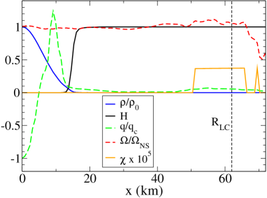
Figure 1: Aligned rotator. Several quantities displayed in the equatorial plane as a function of the cylindrical radius after two rotational periods. The kernel function $H$ indicates the value of the density at which the current changes abruptly. The EM quantities do not display any significant discontinuity in that region, as can be appreciated for instance in the charge density. The magnetic fields in the magnetosphere, up to the light cylinder, co-rotates with the frequency of the star $\Omega_{NS}$. The anomalous resistivity appears only in the regions with $E>B$, close and beyond the light cylinder.

We consider first the evolution of an uniformly rotating stable star of mass $M=1.58M_{\odot}$ and equatorial/polar radius $R=16.1/10.6~{}{\rm km}$. The star rotates with a period $T=1.3{\rm ms}$, so that the light cylinder is located at $R_{\rm LC}=c/\Omega_{NS}=62~{}{\rm km}$. The strength of the magnetic field at the pole is $B_{p}=1.8\times 10^{14}G$. The numerical domain extends up to $L=300~{}{\rm km}$ and contains four centered FMR grids with decreasing sizes (and twice better resolved) such that the highest resolution grid has $\Delta x=0.76~{}{\rm km}$ and extends up to $76~{}{\rm km}$ (i.e., beyond the light cylinder).

This initial configuration is evolved until that the solution relaxes to a quasi-stationary state. Different quantities are plotted along the equatorial plane in fig. 1 and that both the initial and the final magnetic field solutions are displayed in fig. 2. The relaxed final state has the characteristic features observed in previous works. The magnetic fields are being dragged by the fluid rotation in the interior of the star (i.e., as in the initial state), producing a tension that forces the magnetic fields in the magnetosphere to co-rotate with the star up to the light cylinder. Beyond this surface, the magnetic field lines open up, creating a current sheet in the equatorial plane where the anomalous resistivity in the current (or bringing back the neglected fluid inertia) is necessary to preserve the physical condition $B^{2}>E^{2}$.

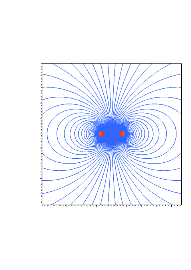
Figure 2: Aligned rotator. The fluid density, the magnetic field –poloidal components in lines and toroidal one in colors– and the coefficient $\chi$ of the anomalous conductivity on the $x=0$ plane at $t=0$ and after two rotational periods of the star. The relaxed solution exhibits the known properties of the aligned rotator solution, namely an opening of the magnetic field lines roughly at the expected position $R_{\rm LC}\approx 4.0\,R_{s}$. These plots do not show the entire computational domain.

We have computed the Poynting-vector luminosity at two surfaces at $R_{ext}=\{76,114\}~{}{\rm km}$ located outside the light cylinder, where the measures converge to a unique well-defined value. The EM radiation is mainly dipolar (i.e., around $90\%$ of the energy), with a small fraction in higher multipoles. The luminosity can be compared with previous results in flat spacetime geometry where the spherical star is modeled through inner boundary conditions (Contopoulos & Spitkovsky, 2006; Spitkovsky, 2006)

$$L_{\rm sd}={1\over 4}B_{\rm pole}^{2}R_{\rm NS}^{2}c\left({\Omega_{\rm NS}R_{\rm NS}\over c}\right)^{4}~{}.$$ (85)

Our results agrees within a difference of $\approx 20\%$, where we have used $R_{\rm NS}=R_{eq}$. It is unclear where this small disagreement may come from, since there are several possible explanations; the ambiguity in the definition of the radius of oblated stars, an excess of dissipation in the current sheet, or purely strong gravitational effects, which may become important due to the high compactness $M/R=0.125$ of the star.

We have also monitored both the energy-momentum constraints and the divergence constraints, checking that they remain small and under control during the evolution. In particular, $|\nabla\cdot B|/|B|\leq 0.05$ in all the domain but the current sheet. By comparing the solutions obtained with three different resolutions, each one improving a factor $1.18$ the previous space discretization $\Delta x$, we have observed that the code converges at $1.8$-order. The luminosity for these three resolutions displayed in fig. 3 shows that, in spite of the spasmodic reconnections happening in the current sheet, the system converges to a quasi-stationary solution with a steady luminosity.

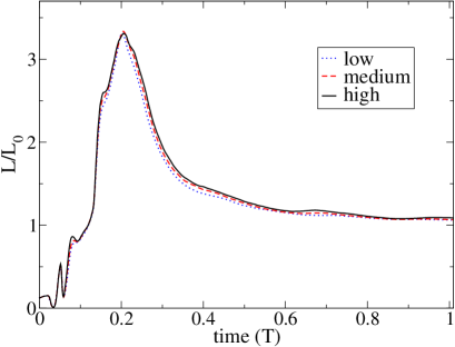
Figure 3: Aligned rotator. The EM luminosity as a function of the rotational period for three different resolutions $\Delta x=\{0.76,0.64,0.55\}{\rm km}$, showing the initial transient followed by a fast decay to the quasi-stationary solution. The luminosity has been normalized with respect to the asymptotic value, reached approximately after $2$ rotational periods, of the low resolution simulation.

6.2 Collapse of a magnetized rotating neutron star

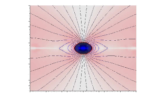
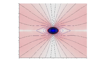
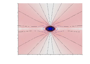
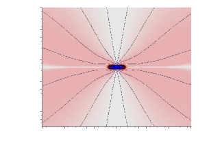
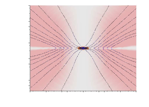
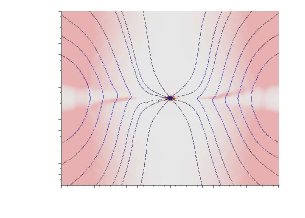
Figure 4: Collapse of a magnetized rotating star. The fluid density, the Poynting flux density and the poloidal magnetic field in the $x=0$ plane representative stages of the collapse corresponding to $t=\{-0.43,-0.30,-0.18,-0.05,0.08,0.20\}$ ms.

After assessing the validity of our implementation with the aligned rotator solution, we can consider a more challenging and dynamical case; the collapse of an uniformly rotating magnetized neutron star to a black hole. The initial data is the same as it was considered in (Lehner et al., 2011); a star lying on the unstable branch with mass $M=1.84M_{\odot}$ and equatorial/polar radius $R=10.6/7.3~{}{\rm km}$, rotating with a period $T=0.78{\rm ms}$ so that the light cylinder is located at $R_{\rm LC}=37~{}{\rm km}$. The strength of the magnetic field at the pole is chosen to be $B_{p}=1.8\times 10^{11}G$, although the results may be rescaled to any strength as long as the magnetic pressure is much smaller than the fluid one. The numerical domain extends up to $L=300~{}{\rm km}$ and contains $6$ centered FMR grids with decreasing sizes such that the highest resolution grid has $\Delta x=0.19~{}{\rm km}$ and extends up to $21~{}{\rm km}$, while that the second highest extends up to $44~{}{\rm km}$, beyond the initial location of the light cylinder.

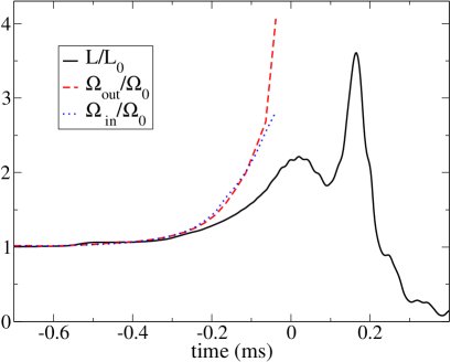
Figure 5: Collapse of a magnetized rotating star. The EM luminosity and the angular frequency of the magnetic field – computed inside and outside the star– as a function of time. These quantities have been normalized with respect to some reference values, calculated once the system relaxes to a quasi-steady state (i.e., the aligned rotator solution) at early times. The agreement between the interior and the exterior angular velocity shows that it is being propagated correctly through the surface of the star.

Small perturbations arising from numerical truncation errors are enough to trigger the collapse of the unstable star. The horizon appears after around $1ms$, although the most dynamical part only stands for the last $0.1ms$, ending when all the matter disappears beyond the horizon and the nearby magnetic fields reconnects in the equatorial plane and escapes to infinity. The conservation of angular momentum implies that the angular velocity of the star increases during the collapse, dragging the magnetic field lines in the magnetosphere and bringing the light cylinder closer to the star. The magnetic fields also grow due to the magnetic flux conservation. Once all the fluid has accreted onto the black hole, the magnetic fields looses their anchorage, reconnects and propagates away from the source. A significant fraction of the energy stored in the magnetosphere is radiated to infinity in this burst. The density of the star, the Poynting vector density $|\Phi_{2}|^{2}$ and the magnetic fields are displayed at some representative stages of the collapse in fig. 4.

The growth of the angular velocity and the magnetic field implies that the luminosity of the aligned rotator (85) during a quasi-adiabatic collapse will increase as  $L_{0}(R_{\rm NS}/R)^{6}$ (Lyutikov, 2011), being $L_{0}$ the initial luminosity of the star. However, since the collapse time is shorter than the star’s period, the outer part of the magnetosphere is not able to respond to the changes in the start’s surface, reducing the power of the luminosity to $(R_{\rm NS}/R)^{4}$ (Lehner et al., 2011). In addition, strong gravitational effects will soften the growth of both the angular frequency and the radial magnetic field, leading to a much more moderate luminosity growth.

We have computed the electromagnetic luminosity in a sphere located at $R_{ext}=76~{}{\rm km}$, beyond the light cylinder. The EM radiation is mainly dipolar and grows during the collapse, with a strong burst due to the reconnection when the fluid is completely swallowed by the black hole. The luminosity and the angular velocity – computed inside and outside the star– are displayed in figure 5. The energy in the magnetosphere increases by a factor $C_{peak}\approx 2$ during the collapse. The total radiated energy can be expressed as a fraction $\epsilon_{\rm rad}$ of the peak energy $C_{peak}E_{dipole,0}$, namely

$$E_{\rm rad}\approx 1.4\times 10^{47}\,C_{\rm peak}\,\epsilon_{\rm rad}\left(\frac{B_{p}}{10^{15}G}\right)^{2}\,{\rm erg}.$$ (86)

where we have used $E_{\rm dipole,0}=1.4\times 10^{47}B_{\rm pole,15}^{2}\,{\rm erg}$ for a star of radius $R_{NS}\approx 12~{}{\rm km}$  (Lehner et al., 2011). In our simulation we have found $\epsilon_{\rm rad}=0.6$, implying that the system radiates $E_{\rm rad}\approx 1.6\times 10^{47}$ergs during the collapse (for a magnetic field of $10^{15}$G). Notice that this value is different from the analytical estimates and indicates the importance of the fast dynamic and strong gravitational effects in this scenario.

7 Summary

We have presented a formulation of the general relativistic resistive MHD equations. We have discussed different generalizations of the isotropic Ohm’s law, and constructed a phenomenological current such that the system reduces either to the ideal MHD limit or to the force-free approximation just by changing the ratio of isotropic/anisotropic conductivities. We have explained how to deal with the potential stiffness of the equations by using the implicit-explicit Runge-Kutta methods, showing how to perform the implicit evolution of the electric field and the recovery of the primitive from the conserved fields at the same time for any algebraic Ohm’s law. We implemented the formulation within the HAD computational infrastructure and revisited two interesting astrophysical problems; the aligned rotator and the collapse of a rotating neutron star to a black hole. None of these cases has a known analytical solution, although the first case has been studied extensively. We find a reasonable agreement between our results and previous studies of the aligned rotator, recovering the same qualitative features and approximately the same electromagnetic luminosity.

The case of the collapsing star is more challenging and has been only studied previously either assuming an electrovacuum magnetosphere and/or by matching the exterior to the interior solution. Our results are qualitatively similar to those found in (Lehner et al., 2011), although the total radiated energy in our simulations is one order of magnitude larger due to an increase in both the peak energy in the magnetosphere and the fraction of radiated energy. The possible detectability of this burst has been already discussed in detail in (Lehner et al., 2011) and therefore will not be repeated here.

In conclusion, the resistive MHD framework allows to consider a broad range of new phenomena;study reconnections and dissipation with more realistic Ohm’s law - like the resistive solutions of pulsar magnetospheres (Li et al., 2012)-, model the magnetic growth due to different instabilities by using the mean-field dynamo (Bucciantini & Del Zanna, 2012), and compute the magnetosphere interaction of binary systems –like neutron-neutron stars and neutron-black hole–, which may be crucial to study the possible electromagnetic counterparts to the gravitational waves emitted by these systems, among others possibilities. Work on these directions is in progress and it will be reported in the near future.

Appendix A IMEX

IMEX Runge-Kutta schemes can be represented by a double tableau in the usual Butcher notation (Butcher, 1987, 2003)

$${\tilde{c}}$$

          (87)

where the coefficients $\tilde{c}$ and $c$ used for the treatment of non-autonomous systems are given by the following relation

$${\tilde{c}}_{i}=\sum_{j=1}^{i-1}~{}{\tilde{a}}_{ij}~{}~{}~{},~{}~{}~{}{c}_{i}=\sum_{j=1}^{i}~{}{a}_{ij}~{}~{}~{}.$$ (88)

Solutions of conservation equations have some norm that decreases in time. It would be desirable, in order to avoid spurious numerical oscillations arising near discontinuities of the solution, to maintain such property at a discrete level by the numerical method. The most commonly used norms are the TV-norm and the infinity norm. A scheme is called Strong Stability Preserving (SSP) if maintains a given norm during the evolution (Spiteri & Ruuth, 2002).

In all these schemes the implicit tableau corresponds to an L-stable scheme (that is, $\omega^{T}A^{-1}e=1$, being $e$ a vector whose components are all equal to $1$), whereas the explicit tableau is SSP$k$, where $k$ denotes the order of the SSP scheme. We shall use the notation SSP$k(s,\sigma,p)$, where the triplet $(s,\sigma,p)$ characterizes the number of $s$ stages of the implicit scheme, the number $\sigma$ of stages of the explicit scheme and the order $p$ of the IMEX scheme.

There are different IMEX RK schemes available in the literature. We have considered only third order IMEX schemes, some of them found in the literature (Pareschi & Russo, 2005) and others developed by us. All of them are based on a third order SSP explicit scheme that can be implemented efficiently by using only two levels of fields and one of rhs. It is worth mentioning that these methods are still under development and have few drawbacks. Probably the most serious one is an accuracy degradation for some range of the relaxation time $\epsilon$.

Table 1: Tableau for the explicit (left) implicit (right) IMEX-SSP3(4,3,3) L-stable scheme

0	0	0	0	0
0	0	0	0	0
1	0	1	0	0
1/2	0	1/4	1/4	0
	0	1/6	1/6	2/3

$\alpha$	$\alpha$	0	0	0
0	-$\alpha$	$\alpha$	0	0
1	0	$1-\alpha$	$\alpha$	0
1/2	$\beta$	$\eta$	$1/2-\beta-\eta-\alpha$	$\alpha$
	0	1/6	1/6	2/3

$$\alpha=0.24169426078821~{},~{}\beta=0.06042356519705~{},~{}\eta=0.12915286960590$$

Table 2: Tableau for the explicit (left) implicit (right) IMEX-SSP3(5,3,3) L-stable scheme

0	0	0	0	0	0
0	0	0	0	0	0
1	0	1	0	0	0
1/2	0	1/4	1/4	0	0
1	0	1/6	1/6	2/3	0
	0	1/6	1/6	2/3	0

$\alpha$	$\alpha$	0	0	0	0
0	-$\alpha$	$\alpha$	0	0	0
1	0	$1-\alpha$	$\alpha$	0	0
1/2	$a_{41}$	$a_{42}$	$a_{43}$	$\alpha$	0
1	0	1/6	0	2/3	1/6
	0	1/6	0	2/3	1/6

$$a_{41}=\frac{1}{8\alpha}(2\alpha^{2}+2\alpha-1)~{}~{},~{}~{}a_{42}=\frac{1}{8\alpha}(-4\alpha^{2}+1)~{}~{},~{}~{}a_{43}=\frac{1}{4}(-3\alpha+1)~{}~{},~{}~{}\alpha=1/3~{}~{}.$$

Appendix B Ideal MHD limit

The ideal MHD limit can be obtained by requiring the current to be finite even in the limit of infinite isotropic conductivity, leading to the condition $E^{i}=-\epsilon^{ijk}v_{j}B_{k}$. The Ohm’s law current becomes undetermined (i.e., an infinite conductivity multiplying a vanishing electric field in the co-moving frame), but it can still be computed from the redundant Maxwell equation for the electric field evolution (2.2). The evolution of the magnetic field can be simplified by substituting the ideal MHD condition in (2.2),

$$\partial_{t}(\sqrt{\gamma}B^{i}) + \partial_{k}[\sqrt{\gamma}\{(\alpha v^{k}-\beta^{k})B^{i}-\alpha v^{i}B^{k}+\alpha\gamma^{ki}\phi\}]$$ (89)

$$= \sqrt{\gamma}[-B^{k}\partial_{k}\beta^{i}+\phi\gamma^{ik}(\partial_{k}\alpha+\Gamma^{j}_{jk})]$$

The transformation from conserved to primitive is simplified by eliminating the electric field as an independent variable and may allow us to recover the primitive quantities in a more robust way. Substituting the ideal MHD condition in the definition of the conserved variables

$$\tau = hW^{2}+B^{2}-p-D-\frac{1}{2}[(B^{k}v_{k})^{2}+\frac{B^{2}}{W^{2}}]~{}~{}~{},~{}~{}~{}$$ (90)

$$S_{i} = [hW^{2}+B^{2}]v_{i}-(B^{k}v_{k})B_{i}~{}~{}~{}.$$ (91)

it is easy to check that

$$v_{i}B^{i}=\frac{S_{i}B^{i}}{hW^{2}}~{}~{}.$$ (92)

Using this relation, the scalar product $S^{i}S_{i}$ can be solved for the Lorentz factor, obtaining

$$c\equiv\frac{1}{W^{2}}=1-\frac{x^{2}S^{2}+(2x+B^{2})(S_{i}B^{i})^{2}}{x^{2}(x+B^{2})^{2}}$$ (93)

Assuming an ideal gas EoS, and after some manipulations in the definition of $\tau$ (90), the resulting final equation to solve is

$$f(x) = [1-\frac{(\Gamma-1)c}{\Gamma}]x+[\frac{(\Gamma-1)\sqrt{c}}{\Gamma}-1]D$$ (94)

$$+ [1-\frac{c}{2}]B^{2}-\frac{1}{2x^{2}}(S_{i}B^{i})^{2}-\tau~{}~{}.$$

References

- Alic et al. (2012) Alic D., Moesta P., Rezzolla L., Zanotti O., Jaramillo J. L., 2012, Astrophysical Journal, 754, 36
- Anderson et al. (2006) Anderson M., Hirschmann E., Liebling S. L., Neilsen D., 2006, Class. Quant. Grav., 23, 6503
- Anderson et al. (2008) Anderson M., et al., 2008, Phys. Rev., D77, 024006
- Andersson (2012) Andersson N., 2012, ArXiv e-prints
- Balbus & Hawley (1991) Balbus S. A., Hawley J. F., 1991, Astrophysical Journal, 376, 214
- Balbus & Hawley (1998) —, 1998, Reviews of Modern Physics, 70, 1
- Baumgarte & Shapiro (2003) Baumgarte T. W., Shapiro S. L., 2003, Astrophys. J., 585, 930
- Bekenstein & Oron (1978) Bekenstein J. D., Oron E., 1978, Physical Review D, 18, 1809
- Blandford & Znajek (1977) Blandford R. D., Znajek R. L., 1977, Mon. Not. R. Astron. Soc., 179, 433
- Bucciantini & Del Zanna (2012) Bucciantini N., Del Zanna L., 2012, ArXiv e-prints
- Bucciantini et al. (2006) Bucciantini N., Thompson T. A., Arons J., Quataert E., Del Zanna L., 2006, MNRS, 368, 1717
- Butcher (1987) Butcher J., 1987
- Butcher (2003) —, 2003
- Campanelli et al. (2006) Campanelli M., Lousto C. O., Marronetti P., Zlochower Y., 2006, Physical Review Letters, 96, 111101
- Contopoulos & Spitkovsky (2006) Contopoulos I., Spitkovsky A., 2006, Astrophysical Journal, 643, 1139
- Dedner et al. (2002) Dedner A., Kemm F., Kröner D., Munz C.-D., Schnitzer T., Wesenberg M., 2002, Journal of Computational Physics, 175, 645
- Dionysopoulou et al. (2012) Dionysopoulou K., Alic D., Palenzuela C., Rezzolla L., Giacomazzo B., 2012, ArXiv e-prints
- Dumbser & Zanotti (2009) Dumbser M., Zanotti O., 2009, Journal of Computational Physics, 228, 6991
- Goldreich & Julian (1969) Goldreich P., Julian W. H., 1969, Astrophys.J., 157, 869
- Gruzinov (2007) Gruzinov A., 2007, Astrophys. J., 667, L69
- Hawley & Balbus (1991) Hawley J. F., Balbus S. A., 1991, Astrophysical Journal, 376, 223
- Hawley et al. (1995) Hawley J. F., Gammie C. F., Balbus S. A., 1995, Astrophysical Journal, 440, 742
- Kalapotharakos & Contopoulos (2009) Kalapotharakos C., Contopoulos I., 2009, Astronomy and Astrophysics, 496, 495
- Komissarov (2004) Komissarov S. S., 2004, MNRS, 350, 427
- Komissarov (2007) —, 2007, Mon. Not. R. Astron. Soc., 382, 995
- Lehner et al. (2006) Lehner L., Liebling S. L., Reula O., 2006, Class. Quant. Grav., 23, S421
- Lehner et al. (2011) Lehner L., Palenzuela C., Liebling S. L., Thompson C., Hanna C., 2011, ArXiv e-prints
- Li et al. (2012) Li J., Spitkovsky A., Tchekhovskoy A., 2012, Astrophysical Journal, 746, 60
- Liebling (2002) Liebling S. L., 2002, Phys. Rev. D, 66, 041703
- Lyutikov (2011) Lyutikov M., 2011, Physical Review D, 83, 124035
- McKinney (2006) McKinney J. C., 2006, Mon. Not. Roy. Astron. Soc. Lett., 368, L30
- Moesta et al. (2012) Moesta P., Alic D., Rezzolla L., Zanotti O., Palenzuela C., 2012, Astrophys. J., 749, L32
- Neilsen et al. (2011) Neilsen D., Lehner L., Palenzuela C., Hirschmann E. W., Liebling S. L., Motl P. M., Garrett T., 2011, Proceedings of the National Academy of Science, 108, 12641
- Newman & Penrose (1962) Newman E., Penrose R., 1962, J.Math.Phys., 3, 566
- Obergaulinger et al. (2010) Obergaulinger M., Aloy M. A., Müller E., 2010, Astronomy and Astrophysics, 515, A30
- Palenzuela et al. (2011) Palenzuela C., Bona C., Lehner L., Reula O., 2011, Classical and Quantum Gravity, 28, 134007
- Palenzuela et al. (2010a) Palenzuela C., Garrett T., Lehner L., Liebling S. L., 2010a, Physical Review D, 82, 044045
- Palenzuela et al. (2010b) Palenzuela C., Lehner L., Liebling S. L., 2010b, Science, 329, 927
- Palenzuela et al. (2009) Palenzuela C., Lehner L., Reula O., Rezzolla L., 2009, MNRS, 394, 1727
- Palenzuela et al. (2010c) Palenzuela C., Lehner L., Yoshida S., 2010c, Physical Review D, 81, 084007
- Pareschi & Russo (2005) Pareschi L., Russo G., 2005, J. Sci. Comput., 25, 112
- Pretorius (2002) Pretorius F., 2002, PhD thesis, The University of British Columbia
- Price & Rosswog (2006) Price D. J., Rosswog S., 2006, Science, 312, 719
- Spiteri & Ruuth (2002) Spiteri R., Ruuth S., 2002, SIAM J. Numer. Anal., 40(2), 469
- Spitkovsky (2006) Spitkovsky A., 2006, Astrophys. J., 648, L51
- Takamoto & Inoue (2011) Takamoto M., Inoue T., 2011, Astrophysical Journal, 735, 113
- Tchekhovskoy & Spitkovsky (2012) Tchekhovskoy A., Spitkovsky A., 2012, ArXiv e-prints
- Uzdensky (2011) Uzdensky D. A., 2011, Space Science Reviews, 160, 45
- Zanotti & Dumbser (2011) Zanotti O., Dumbser M., 2011, MNRS, 418, 1004
- Zenitani et al. (2010) Zenitani S., Hesse M., Klimas A., 2010, Astrophys. J., 716, L214