Cosmological Evolution of Interacting New Holographic Dark Energy in Non-flat Universe

Abstract

We consider the interacting holographic dark energy with new infrared cutoff (involving Hubble parameter and its derivative) in non-flat universe. In this context, we obtain the equation of state parameter which evolutes the universe from vacuum dark energy region towards quintessence region for particular values of constant parameters. It is found that this model always remains unstable against small perturbations. Further, we establish the correspondence of this model having quintessential behavior with quintessence, tachyon, K-essence and dilaton scalar field models. The dynamics of scalar fields and potentials indicate accelerated expansion of the universe which is consistent with the current observations. Finally, we discuss the validity of the generalized second law of thermodynamics in this scenario.

Keywords: New holographic dark energy; Dark matter; Scalar field models; Generalized second law of thermodynamics.
PACS: 95.36.+x; 95.35.+d; 11.10.-z; 98.80.-k.

1 Introduction

Dark energy (DE) is one of the most attractive and active fields in modern cosmology due to the indications of accelerated expansion of the universe through type Ia Supernovae [1]. Observational data like CMBR [2], large scale structure [3, 4], gravitational lensing surveys [5] and galaxy redshift surveys [6] also favor this phenomenon. However, the identity of DE is still ambiguous and various models have been suggested to know its nature. Its simplest candidate is the cosmological constant but it suffers two well-known problems, i.e., ”fine tuning problem” and ”cosmic coincidence problem” [7].

In order to understand the nature of DE phenomenon, various dynamical DE models have been proposed which can be characterized by the equation of state (EoS) parameter $\omega$. The holographic dark energy (HDE) is one of the emergent dynamical DE model proposed in the context of fundamental principle of quantum gravity, so called holographic principle [8]. It is derived with the help of entropy-area relation of thermodynamics of black hole horizons in general relativity which is also known as the Bekenstein-Hawking entropy bound, i.e., $S\simeq M^{2}_{p}L^{2}$, where $S$ is the maximum entropy of the system of length $L$ and $M_{p}=(8\pi G)^{-\frac{1}{2}}$ is the reduced Planck mass. Using this relation, Cohen et al. [9] argued that the vacuum energy (or the quantum zero-point energy) of a system with size $L$ should always remain less than the mass of a black hole with the same size due to the formation of black hole in quantum field theory. Hsu [10] and Li [11] formulated this statement in mathematical form as

$$\rho_{\Lambda}=\frac{3m^{2}}{8\pi GL^{2}},$$

which is known as HDE density, $m$ is constant, $L$ is the infrared (IR) cutoff and $G$ is the gravitational constant.

The density of HDE describes the connectivity between ultraviolet (UV) and IR cutoffs which represent the bounds of energy density and size of the universe, respectively. The HDE model suffers the choice of IR cutoff problem. Li [11] proved that Hubble as well as particle horizons are not compatible with the present status of the universe while the future event horizon is the best candidate for non-interacting HDE with suitable parameter $m$. It is argued [12] that HDE with future event horizon plagued with causality problem (why should we calculate the current value of DE density with the help of future event horizon of the universe$?$). This problem motivated people [12]-[14] to modify the IR cutoff as a function of the Ricci scalar or generalized form of the Ricci scalar. Further, observational analysis has also been done for these types of HDE models [15].

The stability against small perturbations is a well-known procedure to check the viability of a DE model. For this purpose, the sign of the square of the speed of sound, $\upsilon^{2}_{s}=\frac{dp_{\Lambda}}{d\rho_{\Lambda}}$, plays a key role - its negativity represents instability and vice versa [7]. It was shown [16] that Chaplygin and tachyon Chaplygin gases are stable as $\upsilon^{2}_{s}>0$. However, for the holographic [17], agegraphic [18] and QCD ghost DE [19] models, $\upsilon^{2}_{s}<0$, i.e., they are classically unstable.

The scalar-field dark energy model then can be considered as an effective description of this holographic theory. The reconstruction of HDE in terms of scalar fields has been discussed widely. The scalar fields (which naturally occur in particle physics such as string theory [20]) are used as a possible candidate of DE. In this scenario, a large number of models have been proposed including quintessence, phantom, K-essence, tachyon, ghost condensates and dilatonic DE [20, 21] etc. Granda and Oliveros [22] formulated the scalar field models for HDE by using new IR cutoff [13] (called new HDE (NHDE)) in flat FRW universe. Karami and Fehri [23] generalized this work to the non-flat universe. Recently, Sheykhi [24] has constructed the quintessence, tachyon, K-essence and dilatonic DE scalar field models for interacting HDE with Hubble horizon as an IR cutoff in flat universe. The generalized second law of thermodynamics (GSLT) was also discussed for HDE model with different IR cutoff for non-flat universe [25].

It is believed that an early inflation era provides a flat universe, but this consequence is only true if the number of e-foldings is very large [26]. The data of first year WMAP analysis favors the non-flat scenario of the universe [27]. Also, different observational data provided the evidence about the contribution of spatial curvature to the total energy density of the universe [28]-[34]. It was shown that the parameterizations of the dark energy models admit the non-flat universe by implying compatible observational data [35]. Recently, Lu et al. [36] have used type Ia supernovae, baryon acoustic oscillations, CMBR and observational Hubble data and obtained the value $-0.0013^{+0.0130}_{-0.0040}$ for fractional energy density due to curvature. It would be interesting to study the universe with a spatial curvature.

In view of above discussion, we extend the work of Sheykhi [24] by taking the generalized form of IR cutoff of HDE in non-flat universe. We also check the validity of the GSLT in this scenario. The paper is organized as follows: Section 2 contains the discussion of the evolution and instability of interacting NHDE in non-flat universe. Section 3 is devoted for the reconstruction of scalar field models of interacting NHDE while section 4 investigates the validity of GSLT. The last section provides the summary of our results.

2 New Holographic Dark Energy

In this section, we manipulate the expressions of EoS parameter and speed of sound for NHDE interacting with dark matter (DM) in non-flat FRW universe

$$ds^{2}=-dt^{2}+a^{2}(t)[\frac{dr^{2}}{1-kr^{2}}+r^{2}(d\theta^{2}+\sin\theta^{2}d\phi^{2})].$$ (1)

Here $a(t)$ is the cosmic scale factor which measures the expansion of the universe and $k=-1,0,1$ represents the spatial curvature indicating the open, flat and closed universes, respectively. The corresponding equations of motion are

$$H^{2}+\frac{k}{a^{2}} = \frac{1}{3}(\rho_{m}+\rho_{\Lambda}),$$ (2)

$$\dot{H}+H^{2} = -\frac{1}{6}(\rho_{m}+\rho_{\Lambda}+3p_{\Lambda}),$$ (3)

here we assume $8\pi G=1$ as well as dust like DM. Also, $\rho_{m}$ and $\rho_{\Lambda}$ are DM and DE densities, $p_{\Lambda}$ is pressure due to DE, $H$ denotes the Hubble parameter and dot represents derivative with respect to time. We can rewrite Eq.(3) in the form of fractional energy densities as

$$\Omega_{m}+\Omega_{\Lambda}=1+\Omega_{k},$$ (4)

where

$$\Omega_{m}=\frac{\rho_{m}}{3H^{2}},\quad\Omega_{\Lambda}=\frac{\rho_{\Lambda}}{3H^{2}},\quad\Omega_{k}=\frac{k}{a^{2}H^{2}}.$$

We assume the NHDE density in the following form [13]

$$\rho_{\Lambda}=3(\mu H^{2}+\lambda\dot{H}),$$ (5)

where $\mu$ and $\lambda$ are positive constants.

The interaction of DM and NHDE leads to the equation of continuity in the form of two non-conserving equations as

$$\dot{\rho}_{m}+3H\rho_{m} = \Upsilon,$$ (6)

$$\dot{\rho}_{\Lambda}+3H(\rho_{\Lambda}+p_{\Lambda}) = -\Upsilon.$$ (7)

We choose the following form of the interaction term $\Upsilon$

$$\Upsilon=3d^{2}H\rho_{m},$$ (8)

here $d^{2}$ is the interacting constant. Using Eqs.(6) and (8), we obtain DM density as follows

$$\rho_{m}=\rho_{m_{0}}e^{-3(1-d^{2})x},$$ (9)

where $x=\ln a$ and $\rho_{m_{0}}$ is an integration constant. Inserting Eqs.(5) and (9) in Eq.(2), we obtain the differential equation

$$\frac{dE^{2}}{dx}+\frac{2(\mu-1)}{\lambda}E^{2}=\frac{2\Omega_{k_{0}}}{\lambda}e^{-2x}-\frac{2\Omega_{m_{0}}}{\lambda}e^{-3(1-d^{2})x},$$ (10)

where $E^{2}=\frac{H^{2}}{H^{2}_{0}},~{}(0)$ represents the present value of the parameter and $b$ is an integration constant. This has the solution

$$E^{2}=\frac{\Omega_{k_{0}}}{\mu-\lambda-1}e^{-2x}-\frac{2\Omega_{m_{0}}}{2(\mu-1)-3(1-d^{2})\lambda}e^{-3(1-d^{2})x}+be^{-\frac{2}{\lambda}{(\mu-1)x}}.$$ (11)

The initial condition $a_{0}=1$ yields $x=0,~{}E=1$, and hence we have

$$b=1-\frac{\Omega_{k_{0}}}{\mu-\lambda-1}+\frac{2\Omega_{m_{0}}}{2(\mu-1)-3(1-d^{2})\lambda}.$$ (12)

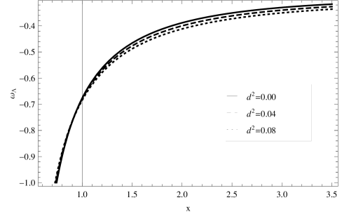
Figure 1: Plot of $\omega_{\Lambda}$ versus $x$ for NHDE.

With the help of Eqs.(5), (7) and (11), we obtain the evolution parameter of interacting NHDE as

$$\omega_{\Lambda} = \left[\frac{(\lambda-\mu)\Omega_{k_{0}}}{3(\mu-\lambda-1)}e^{-2x}+\frac{2d^{2}\Omega_{m_{0}}}{2(\mu-1)-3(1-d^{2})\lambda}e^{-3(1-d^{2})x}-\frac{b}{3\lambda}\right.$$ (13)

$$\times \left.(3\lambda-2\mu+2)e^{\frac{-2(\mu-1)x}{\lambda}}\right]\left[\frac{(\mu-\lambda)\Omega_{k_{0}}}{(\mu-\lambda-1)}e^{-2x}-(2\mu-3(1-d^{2})\lambda)\right.$$

$$\times \left.(2(\mu-1)-3(1-d^{2})\lambda)^{-1}\Omega_{m_{0}}e^{-3(1-d^{2})x}+be^{\frac{-2(\mu-1)x}{\lambda}}\right]^{-1}.$$

We plot the EoS parameter $\omega_{\Lambda}$ versus $x$ with respect to different well-known choices of interacting parameter $d^{2}$, i.e., 0, 0.04, 0.08 shown in Figure 1. Also, we assume the NHDE parameters as $\mu=1.198,~{}\lambda=0.195$ and the current values of $\Omega_{k_{0}}=0.01,~{}\Omega_{\Lambda_{0}}=0.73$. We see that the EoS parameter translates the universe from vacuum DE region towards quintessence region.

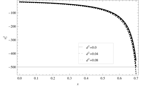
Figure 2: Plot of $\upsilon_{s}^{2}$ versus $x$ for NHDE.

The speed of sound is given by [7]

$$\upsilon_{s}^{2}=\frac{\dot{p}}{\dot{\rho}}=\frac{p^{\prime}}{\rho^{\prime}},$$ (14)

where prime means differentiation with respect to $x$. Using Eqs.(5), (7), (11) and (14), it follows that

$$\upsilon^{2}_{s} = \left[\frac{2(\mu-\lambda)\Omega_{k_{0}}}{3(\mu-\lambda-1)}e^{-2x}-\frac{6d^{2}(1-d^{2})\Omega_{m_{0}}}{2(\mu-1)-3(1-d^{2})\lambda}e^{-3(1-d^{2})x}+2b(\mu-1)\right.$$ (15)

$$\times \left.\frac{(3\lambda-2\mu+2)}{3\mu^{2}}e^{\frac{-2(\mu-1)x}{\lambda}}\right]\left[\frac{-2(\mu-\lambda)\Omega_{k_{0}}}{(\mu-\lambda-1)}e^{-2x}+(2\mu-3(1-d^{2})\lambda)\right.$$

$$\times \left.3(1-d^{2})(2(\mu-1)-3(1-d^{2})\lambda)^{-1}\Omega_{m_{0}}e^{-3(1-d^{2})x}-\frac{2b(1-\mu)}{\lambda}\right.$$

$$\times \left.e^{\frac{-2(\mu-1)x}{\lambda}}\right]^{-1},$$

which provides the speed of sound for interacting NHDE. This is shown in Figure 2 for the same constant parameters as given above. In this scenario, the speed of sound remains negative with the increase of interacting parameter. This shows that the NHDE is unstable just like non-interacting HDE model with future event horizon [17].

3 Reconstruction of New Holographic Scalar Field Models

Here, we provide the correspondence of the interacting NHDE with quintessence, tachyon, K-essence and dilaton field models in non-flat universe.

3.1 New Holographic Quintessence Model

The ordinary scalar field $\phi$ is governed by quintessence which is minimally coupled with gravity. The energy density and pressure of the quintessence scalar field are defined as [21]

$$\rho_{q}=\frac{1}{2}\dot{\phi}^{2}+V(\phi),\quad p_{q}=\frac{1}{2}\dot{\phi}^{2}-V(\phi),$$ (16)

where $\dot{\phi}^{2}$ and $V(\phi)$ are termed as kinetic energy and scalar potential, respectively. The EoS parameter for this model becomes

$$\omega_{q}=\frac{\dot{\phi}^{2}-2V(\phi)}{\dot{\phi}^{2}+2V(\phi)}.$$

For the correspondence between NHDE and quintessence scalar field, we set $\rho_{q}=\rho_{\Lambda}$ and $p_{q}=p_{\Lambda}$. Consequently, Eq.(16) yields

$$\dot{\phi}^{2} = 3H^{2}_{0}\left[\frac{2(\mu-\lambda)\Omega_{k_{0}}}{3(\mu-\lambda-1)}e^{-2x}-\frac{(2\mu-3(1-d^{2})\lambda-2d^{2})\Omega_{m_{0}}}{2(\mu-1)-3(1-d^{2})\lambda}e^{-3(1-d^{2})x}\right.$$ (17)

$$+ \left.\frac{2b(\mu-1)}{3\lambda}~{}e^{\frac{-2(\mu-1)x}{\lambda}}\right],$$

$$V(\phi) = 3H^{2}_{0}\left[\frac{2(\mu-\lambda)\Omega_{k_{0}}}{3(\mu-\lambda-1)}e^{-2x}-\frac{(2\mu-3(1-d^{2})\lambda+2d^{2})\Omega_{m_{0}}}{2(2(\mu-1)-3(1-d^{2})\lambda)}e^{-3(1-d^{2})x}\right.$$ (18)

$$+ \left.\frac{b(3\lambda-\mu+1)}{3\lambda}e^{\frac{-2(\mu-1)x}{\lambda}}\right].$$

The kinetic energy can also be written as

$$\phi^{\prime}(a) = \sqrt{3}\left[\frac{2(\mu-\lambda)\Omega_{k_{0}}}{3(\mu-\lambda-1)}e^{-2x}-\frac{(2\mu-3(1-d^{2})\lambda-2d^{2})\Omega_{m_{0}}}{2(\mu-1)-3(1-d^{2})\lambda}e^{-3(1-d^{2})x}\right.$$ (19)

$$+ \left.\frac{2b(\mu-1)}{3\lambda}e^{\frac{-2(\mu-1)x}{\lambda}}\right]^{\frac{1}{2}}\left[{\frac{\Omega_{k_{0}}}{(\mu-\lambda-1)}e^{-2x}-(2\mu-3(1-d^{2})\lambda)}\right.$$

$$\times \left.(2(\mu-1)-3(1-d^{2})\lambda)^{-1}\Omega_{m_{0}}e^{-3(1-d^{2})x}+be^{\frac{-2(\mu-1)x}{\lambda}}\right]^{-\frac{1}{2}}.$$

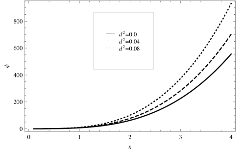
Figure 3: Plot of $\phi$ versus $x$ for quintessence model.

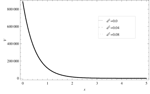
Figure 4: Plot of $V$ versus $x$ for quintessence model.

Figure 5: Plot of $V$ versus $\phi$ for quintessence model.

This equation cannot be solved analytically to obtain $\phi$ due to its complicated nature. To get insights, we solve it numerically and plot $\phi$ against $x$ by choosing initial condition, $\phi(0)=0$, while keeping the remaining parameters same as in the previous section. Figure 3 shows that the scalar field increases (and hence the kinetic energy $\dot{\phi}^{2}$ of the potential decreases) with the passage of time. The potential $V$ versus $x$ and $\phi$ are shown in Figures 4 and 5, respectively, indicating the decreasing behavior. The quintessence potential in terms of $\phi$ shows large value at the present epoch which represents accelerated expansion of the universe. This is consistent with the result shown through phase space analysis [21] that the exponential potential for the scalar field contains the attractor solutions describing the accelerated expansion of the universe. However, in the later time, the universe remains in the accelerated phase because quintessence potential goes to positive and non-zero minima but kinetic energy goes to zero.

3.2 New Holographic Tachyon Model

The tachyon model, originated from the string theory, has been suggested to explain DE scenario. It has an interesting feature that a rolling tachyon interpolates the EoS parameter between $-1$ to $0$. Also, the tachyon model is the best candidate for inflation at high energy. Many attempts have been made to formulate reliable cosmological models with the help of different self-interacting potentials [37]. However, the effective Lagrangian for this model is defined as [21]

$$L=-V(\phi)\sqrt{1+\partial_{\mu}\phi\partial^{\mu}\phi},$$

where $V(\phi)$ represents the tachyon potential. This scalar field has the following energy and pressure

$$\rho_{t}=\frac{V(\phi)}{\sqrt{1-\dot{\phi}^{2}}},\quad p_{t}=-V(\phi)\sqrt{1-\dot{\phi}^{2}}$$ (20)

and the EoS parameter is

$$\omega_{t}=\dot{\phi}^{2}-1.$$ (21)

The correspondence between NHDE and tachyon model is obtained for $\rho_{t}=\rho_{\Lambda}$ and $p_{t}=p_{\Lambda}$ which lead to

$$\dot{\phi}^{2} = \left[\frac{2(\mu-\lambda)\Omega_{k_{0}}}{3(\mu-\lambda-1)}e^{-2x}-\frac{(2\mu-3(1-d^{2})\lambda-2d^{2})\Omega_{m_{0}}}{2(2(\mu-1)-3(1-d^{2})\lambda)}e^{-3(1-d^{2})x}\right.$$ (22)

$$+ \left.\frac{2b(\mu-1)}{3\lambda}e^{\frac{-2(\mu-1)x}{\lambda}}\right]\left[\frac{(\mu-\lambda)\Omega_{k_{0}}}{(\mu-\lambda-1)}e^{-2x}-(2\mu-3(1-d^{2})\lambda)\right.$$

$$\times \left.(2(\mu-1)-3(1-d^{2})\lambda)^{-1}\Omega_{m_{0}}e^{-3(1-d^{2})x}+be^{\frac{-2(\mu-1)x}{\lambda}}\right]^{-1},$$

$$V(\phi) = 3H^{2}_{0}\left[\frac{(\mu-\lambda)\Omega_{k_{0}}}{(\mu-\lambda-1)}e^{-2x}-\frac{(2\mu-3(1-d^{2})\lambda)\Omega_{m_{0}}}{2(\mu-1)-3(1-d^{2})\lambda}e^{-3(1-d^{2})x}\right.$$ (23)

$$+ \left.be^{\frac{-2(\mu-1)x}{\lambda}}\right]^{\frac{1}{2}}\left[\frac{(\mu-\lambda)\Omega_{k_{0}}}{3(\mu-\lambda-1)}e^{-2x}-2d^{2}~{}\Omega_{m_{0}}e^{-3(1-d^{2})x}(2(\mu-1)\right.$$

$$- \left.3(1-d^{2})\lambda)^{-1}+\frac{b}{3\lambda}(3\lambda-2\mu+2)e^{\frac{-2(\mu-1)x}{\lambda}}\right]^{\frac{1}{2}}.$$

From Eqs.(11) and (22), we obtain the kinetic energy term as

$$\phi^{\prime}(a) = \frac{1}{H_{0}}\left[\frac{2(\mu-\lambda)\Omega_{k_{0}}}{3(\mu-\lambda-1)}e^{-2x}-\frac{(2\mu-3(1-d^{2})\lambda-2d^{2})\Omega_{m_{0}}}{2(\mu-1)-3(1-d^{2})\lambda}e^{-3(1-d^{2})x}\right.$$ (24)

$$+ \left.\frac{2b(\mu-1)}{3\lambda}e^{\frac{-2(\mu-1)x}{\lambda}}\right]^{\frac{1}{2}}\left[\frac{(\mu-\lambda)\Omega_{k_{0}}}{(\mu-\lambda-1)}e^{-2x}-(2\mu-3(1-d^{2})\lambda)\right.$$

$$\times \left.(2(\mu-1)-3(1-d^{2})\lambda)^{-1}\Omega_{m_{0}}e^{-3(1-d^{2})x}+be^{\frac{-2(\mu-1)x}{\lambda}}\right]^{-\frac{1}{2}}\left[\Omega_{k_{0}}\right.$$

$$\times \left.(\mu-\lambda-1)^{-1}e^{-2x}-\frac{2\Omega_{m_{0}}e^{-3(1-d^{2})x}}{2(\mu-1)-3(1-d^{2})\lambda}+be^{\frac{-2(\mu-1)x}{\lambda}}\right]^{-\frac{1}{2}}.$$

The plot of the tachyon field $\phi$ versus $x$ is given in Figure 6 which shows that the scalar field $\phi$ increases with the passage of time and becomes steeper for increasing the interacting parameter $d^{2}$. However, the kinetic energy of the tachyon potential decreases and approaches to zero in the future. With this behavior, Eq.(21) indicates the vacuum evolution of the universe. The tachyon potential shows oscillation initially about its maxima (it increases with the increment of $d^{2}$) but approaches to zero in the later time as shown in Figure 7. For the later time, its rapid decrease from maxima gives inverse proportionality to the scalar field. This type of behavior corresponds to scaling solutions in the brane-world cosmology [38].

3.3 New Holographic K-essence Model

Figure 6: Plot of $\phi$ versus $x$ for tachyon model.

Figure 7: Plot of $V$ versus $x$ for tachyon model.

The K-essence model is different from quintessence scalar field model in the sense that it evolutes the universe in the accelerated expansion era. It is originated from the idea of K-inflation which was used to describe the inflation of the early universe at high energies [20]. This model has been used as an alternative candidate of DE which yields interesting results of scaling and attractor solutions [39, 40]. This model is described with a scalar field having non-canonical kinetic energy. The generalized form of scalar field action is [21]

$$S=\int{d^{4}x\sqrt{-g}}p(\phi,\chi),$$

where $p(\phi,\chi)$ shows the pressure density as a function of potential $\phi$ and $\chi=\frac{1}{2}~{}\dot{\phi}^{2}$. The corresponding energy density and pressure are

$$\rho_{k}=V(\phi)(-\chi+3\chi^{2}),\quad p_{k}=V(\phi)(-\chi+\chi^{2}),$$ (25)

where $V(\phi)$ represents the scalar potential of K-essence model. The corresponding EoS parameter is

$$\omega_{k}=\frac{1-\chi}{1-3\chi}.$$ (26)

Equating $\rho_{k}=\rho_{\Lambda}$ and $p_{k}=p_{\Lambda}$ for the correspondence between NHDE and K-essence model, we obtain

$$\chi = \left[\frac{4(\mu-\lambda)\Omega_{k_{0}}}{3(\mu-\lambda-1)}e^{-2x}-\frac{(2\mu-3(1-d^{2})\lambda+2d^{2})\Omega_{m_{0}}}{2(\mu-1)-3(1-d^{2})\lambda}e^{-3(1-d^{2})x}\right.$$ (27)

$$+ \frac{b}{3\lambda}\left.(6\lambda-2\mu+2)e^{\frac{-2(\mu-1)x}{\lambda}}\right]\left[\frac{2(\mu-\lambda)\Omega_{k_{0}}}{(\mu-\lambda-1)}e^{-2x}-(2\mu-3(1-d^{2})\lambda\right.$$

$$+ \left.6d^{2})(2(\mu-1)-3(1-d^{2})\lambda)^{-1}\Omega_{m_{0}}e^{-3(1-d^{2})x}+\frac{b}{\lambda}(4\lambda-2\mu+2)\right.$$

$$\times \left.e^{\frac{-2(\mu-1)x}{\lambda}}\right]^{-1},$$

$$V(\phi) = \frac{3(1-3\omega_{k})^{2}H^{2}_{0}}{2(1-\omega_{k})}\left[\frac{(\mu-\lambda)\Omega_{k_{0}}}{\mu-\lambda-1}e^{-2x}-\frac{(2\mu-3(1-d^{2})\lambda)\Omega_{m_{0}}}{2(\mu-1)-3(1-d^{2})\lambda}\right.$$ (28)

$$\times \left.e^{-3(1-d^{2})x}+be^{\frac{-2(\mu-1)x}{\lambda}}\right].$$

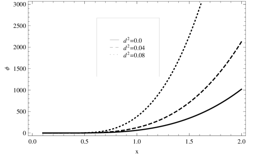
Figure 8: Plot of $\phi$ versus $x$ for K-essence model.

Figure 9: Plot of $\chi$ versus $x$ for K-essence model.

Figure 10: Plot of $V$ versus $\phi$ for K-essence model.

Consequently, the relation $\chi=\frac{1}{2}\dot{\phi}^{2}$ gives the evolution

$$\phi^{\prime}(a) = \frac{\sqrt{2}}{H_{0}}\left[\frac{4(\mu-\lambda)\Omega_{k_{0}}}{3(\mu-\lambda-1)}e^{-2x}-\frac{(2\mu-3(1-d^{2})\lambda+2d^{2})\Omega_{m_{0}}}{2(\mu-1)-3(1-d^{2})\lambda}e^{-3(1-d^{2})x}\right.$$ (29)

$$+ \left.\frac{b(6\lambda-2\mu+2)}{3\lambda}e^{\frac{-2(\mu-1)x}{\lambda}}\right]^{\frac{1}{2}}\left[\frac{2(\mu-\lambda)\Omega_{k_{0}}}{(\mu-\lambda-1)}e^{-2x}-(2\mu-3(1-d^{2})\lambda\right.$$

$$+ \left.6d^{2})(2(\mu-1)-3(1-d^{2})\lambda)^{-1}\Omega_{m_{0}}e^{-3(1-d^{2})x}+\frac{b}{\lambda}(4\lambda-2\mu+2)\right.$$

$$\times \left.e^{\frac{-2(\mu-1)x}{\lambda}}\right]^{-\frac{1}{2}}\left[\frac{\Omega_{k_{0}}}{(\mu-\lambda-1)}e^{-2x}-2\Omega_{m_{0}}e^{-3(1-d^{2})x}(2(\mu-1)\right.$$

$$- \left.3(1-d^{2})\lambda)^{-1}+be^{\frac{-2(\mu-1)x}{\lambda}}\right]^{-\frac{1}{2}}.$$

From here we can plot $\phi$ and $\chi$ versus $x$ with previous assumptions. We see from Figure 8 that the scalar field $\phi$ increases. Figure 9 shows that $\chi$ almost lies in the required interval $\left(\frac{1}{3},\frac{2}{3}\right)$ from early epoch to the later time. The EoS parameter (26) indicates that the accelerated universe can be obtained for this interval. For $\chi<\frac{1}{2}$, it gives phantom DE era which corresponds to late time attractor [39]. Figure 10 shows that $V(\phi)$ increases slowly but attains very large negative value with the increase of scalar field $\phi$.

3.4 New Holographic Dilaton Field

The Lagrangian of dilaton field can be expressed in terms of pressure of scalar field as [20]

$$p_{d}=-\chi+b_{1}e^{b_{2}\phi}\chi^{2},$$ (30)

where $b_{1}$ and $b_{2}$ are taken as positive constants. This Lagrangian (pressure) produces the following energy density

$$\rho_{d} = -\chi+3b_{1}e^{b_{2}\phi}\chi^{2}.$$ (31)

The EoS for dilaton DE is

$$\omega_{d}=\frac{-1+b_{1}e^{b_{2}\phi}\chi}{-1+3b_{1}~{}e^{b_{2}\phi}\chi}.$$ (32)

By setting $\rho_{d}=\rho_{\Lambda}$ and $p_{d}=p_{\Lambda}$, we obtain

$$e^{b_{2}\phi}\chi = \frac{1}{b_{1}}\left[\frac{4(\mu-\lambda)\Omega_{k_{0}}}{3(\mu-\lambda-1)}e^{-2x}-\frac{(2\mu-3(1-d^{2})\lambda+2d^{2})\Omega_{m_{0}}}{2(\mu-1)-3(1-d^{2}\lambda)}e^{-3(1-d^{2})x}\right.$$ (33)

$$+ \left.\frac{b(6\lambda-2\mu+2)}{3\lambda}e^{\frac{-2(\mu-1)x}{\lambda}}\right]\left[\frac{2(\mu-\lambda)\Omega_{k_{0}}}{\mu-\lambda-1}~{}e^{-2x}-\Omega_{m_{0}}e^{-3(1-d^{2})x}\right.$$

$$\times \left.\frac{(2\mu-3(1-d^{2})\lambda+6d^{2})}{2(\mu-1)-3(1-d^{2})\lambda}+\frac{b}{\lambda}(4\lambda-2\mu+2)e^{\frac{-2(\mu-1)x}{\lambda}}\right]^{-1}.$$

The EoS parameter (32) gives the bound of $e^{b_{2}\phi}\chi$ which is $\left(\frac{20}{3},\frac{40}{3}\right)$ in order to obtain the accelerated universe. Its graph versus $x$ with $\alpha=0.05$ is shown in Figure 11 which indicates that this almost lies in the same interval and shows consistency. Also, the solution of (33) follows

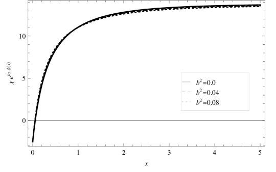
Figure 11: Plot of $e^{b_{2}\phi}\chi$ versus $x$ for dilaton field.

$$\phi(a) = \frac{2}{b_{2}}\ln\left[1+\frac{b_{2}}{\sqrt{2b_{1}H^{2}_{0}}}\int^{x}_{0}\left[\frac{4(\mu-\lambda)\Omega_{k_{0}}}{3(\mu-\lambda-1)}e^{-2x}-\Omega_{m_{0}}e^{-3(1-d^{2})x}\right.\right.$$

$$\times \left.\left.\frac{(2\mu-3(1-d^{2})\lambda+2d^{2})}{2(2(\mu-1)-3(1-d^{2})\lambda)}+\frac{b(6\lambda-2\mu+2)}{3\lambda}e^{\frac{-2(\mu-1)x}{\lambda}}\right]^{\frac{1}{2}}\right.$$

$$\times \left.\left[\frac{2(\mu-\lambda)\Omega_{k_{0}}}{(\mu-\lambda-1)}e^{-2x}-\frac{(2\mu-3(1-d^{2})\lambda+6d^{2})\Omega_{m_{0}}}{2(\mu-1)-3(1-d^{2})\lambda}e^{-3(1-d^{2})x}\right.\right.$$

$$+ \left.\left.\frac{b}{\lambda}(4\lambda-2\mu+2)be^{\frac{-2(\mu-1)x}{\lambda}}\right]^{-\frac{1}{2}}\left[\frac{\Omega_{k_{0}}}{(\mu-\lambda-1)}e^{-2x}-2\Omega_{m_{0}}\right.\right.$$

$$\times \left.\left.(2(\mu-1)-3(1-d^{2})\lambda)^{-1}e^{-3(1-d^{2})x}+be^{\frac{-2(\mu-1)x}{\lambda}}\right]^{-\frac{1}{2}}dx\right].$$ (34)

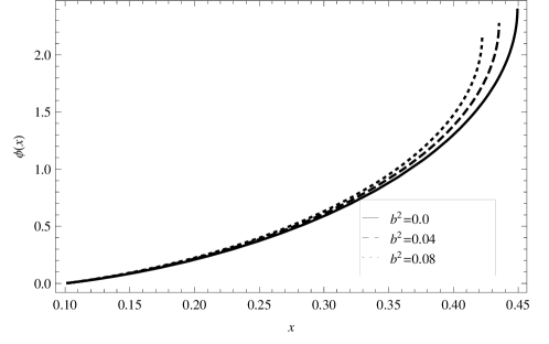
Figure 12: Plot of $\phi$ versus $x$ for dilaton field.

Its graph is shown in Figure 12 which exhibits direct proportionality with respect to $x$. This type of behavior gives scaling solutions for dilaton model as proved in [20].

4 Generalized Second Law of Thermodynamics

In this section, we check the validity of GSLT for interacting NHDE in the non-flat universe. Bekenstein’s [41] provided a relationship about the entropy of black hole horizon and horizon area which plays a crucial role to discuss the GSLT. This law states that the sum of black hole entropy and the background entropy must increase with the passage of time. The first law of thermodynamics yields

$$TdS=pdV+dE,$$ (35)

where $T,~{}S,~{}p,~{}V$ and $E$ denote temperature, entropy, pressure, volume and internal energy of the system, respectively. Differentiating it with respect to time, we obtain

$$\dot{S_{\Lambda}}=\frac{p_{\Lambda}\dot{V}+\dot{E_{\Lambda}}}{T},\quad\dot{S_{m}}=\frac{p_{m}\dot{V}+\dot{E_{m}}}{T},$$ (36)

for the NHDE and DM, respectively. The volume, temperature and entropy of horizon $L$ in non-flat universe are defined as [42]

$$V=\frac{4\pi~{}L^{3}}{3},\quad T=\frac{1}{2\pi L},\quad S_{H}=2\pi^{2}L^{2}.$$ (37)

The internal energies for NHDE and DM are

$$E_{\Lambda}=\frac{4\pi L^{3}\rho_{\Lambda}}{3},\quad E_{m}=\frac{4\pi L^{3}\rho_{m}}{3}.$$ (38)

Using Eqs.(7), (9) and (36)-(38), we have the final expression of the GSLT

$$S^{\prime}_{total} = -\frac{4\pi^{2}}{9\rho^{3}_{\Lambda}}[(1+\omega_{\Lambda})\rho_{\Lambda}+3H^{2}_{0}\Omega_{m_{0}}e^{-3(1-d^{2})x}](\rho^{\prime}_{\Lambda}+2\rho_{\Lambda})-\frac{\pi^{2}\rho^{\prime}_{\Lambda}}{3\rho_{\Lambda}^{2}},$$

where $S^{\prime}_{total}$ denotes the derivative of the sum of entropies due to DM, NHDE and horizon entropy. We plot it against $x$ with the same assumptions as given earlier. Figure 13 shows that the GSLT is valid for early epoch but fails for the later time in this scenario.

Figure 13: Plot of $S^{\prime}_{total}$ versus $x$ for NHDE.

5 Concluding Remarks

It was shown through experimental data that our universe is not totally flat but it contains small positive curvature [26]-[34]. This motivated us to perform the versatile study of the interacting NHDE in the context of non-flat universe. In this paper, we have discussed four main features by choosing different values of interacting parameter i.e., $d^{2}=0,0.04,0.08$ which are summarized as follows. Firstly, we obtain the evolution equation which starts from vacuum DE region $(\omega_{\Lambda}=-1)$ and goes towards quintessence region $(\omega_{\Lambda}>-1)$ as shown in Figure 1. This type of behavior is consistent with the present observations. Secondly, we have discussed the instability of this model against perturbation as shown in Figure 2. It is found that it remains unstable forever like HDE with IR cutoff as a future event horizon [17], agegraphic [18] and ghost QCD [19] DE models but unlike Chaplygin gas [16] DE model.

Thirdly, we have evaluated the interacting NHDE versions of quintessence, tachyon, K-essence and dilaton scalar field DE models. We have also explored the behavior of potentials and dynamics of the scalar field corresponding to these models by using the reliable values of the constant parameters. These are shown in Figures 3-12. It is seen that the scalar field $\phi$ becomes more steeper with the increase of the interacting parameter $d^{2}$ for all scalar field models. Also, the scalar potential $V(\phi)$ decreases more rapidly in case of quintessence for increasing the interacting parameter $d^{2}$ as compared to non-interacting scenario (Figure 5). However, for K-essence model, it increases but achieves a maximum value lower than that of non-interacting case as shown in Figure 10. It was argued [21, 43, 44] that the scalar field models favor the DE phenomenon for EoS parameter lying in the interval $(-1,0)$. However, in our case, the EoS of NHDE remains in this region and shows consistency.

We would like to mention here that our solutions coincide with the attractor solutions (for quintessence [21] and K-essence [39] DE models) and scaling solutions (for tachyon [38] and dilaton [20] DE models). It is remarked that our expressions of EoS parameter and scalar field models can be reduced to the results of [22] (with vanishing of DM density and $k=0$) and of [23] (for the vanishing of DM density only). Finally, we have checked the validity of the GSLT in this scenario. It is found that initially it is valid but fails for the later time.

References

- [1] Perlmutter, S. et al.: Astrophys. J. 517(1999)565.
- [2] Caldwell, R.R. and Doran, M.: Phys. Rev. D 69(2004)103517.
- [3] Koivisto, T. and Mota, D.F.: Phys. Rev. D 73(2006)083502
- [4] Daniel, S.F.: Phys. Rev. D 77(2008)103513.
- [5] Hoekstra, H. and Jain, B.: Ann. Rev. Nucl. Part. Sci. 58(2008)99.
- [6] Fedeli, C., Moscardini, L. and Bartelmann, M.: Astron. Astrophys. 500(2009)667.
- [7] Peebles, P.J.E.: Rev. Mod. Phys. 75(2003)559.
- [8] Susskind, L.: J. Math. Phys. 36(1995)6377.
- [9] Cohen, A., Kaplan, D. and Nelson, A.: Phys. Rev. Lett. 82(1999)4971.
- [10] Hsu, S.D.H.: Phys. Lett. B 594(2004)13.
- [11] Li, M.: Phys. Lett. B 603(2004)1.
- [12] Gao, C., Chen, X. and Shen, Y.G.: Phys. Rev. D 79(2009)043511.
- [13] Granda, L. and Oliveros, A.: Phys. Lett. B 669(2008)275.
- [14] Chen, S. and Jing, J.: Phys. Lett. B 679(2009)144.
- [15] Zhang, X.: Phys. Rev. D 79(2009)103509; Wang, Y. and Xu, L.: Phys. Rev. D 81(2010)083523.
- [16] Gorini, V. et al.: Phys. Rev. D 72(2005)103518; Sandvik, H. et al.: Phys. Rev. D 69(2004)123524.
- [17] Myung, Y.S.: Phys. Lett. B 652(2007)223.
- [18] Kim, K.Y., Lee, H.W. and Myung, Y.S.: Phys. Lett. B 660(2008)118.
- [19] Ebrahimi, E. and Sheykhi, A.: Int. J. Mod. Phys. D 20(2011)2369.
- [20] Piazza, F. and Tsujikawa, S.: JCAP 07(2004)004.
- [21] Copeland, E.J., Sami, M. and Tsujikawa, S.: Int. J. Mod. Phys. D 15(2006)1753.
- [22] Granda, L. and Oliveros, A.: Phys. Lett. B 671(2009)199.
- [23] Karami, K. and Fehri, J.: Phys. Lett. B 684(2010)61.
- [24] Sheykhi, A.: Phys. Rev. D 84(2011)107302.
- [25] Setare, M.R.: JCAP 01(2007)023; Sheykhi, A.: Class. Quantum Grav. 27(2010)025007; Mazumder, M. and Chakraborty, S.: Gen. Relativ. Gravit. 42(2010)813.
- [26] Huang, Q.G. and Li, M.: JCAP 08(2004)013.
- [27] Bennett, C.L. et al.: Astrophys. J. Suppl. 148(2003)1.
- [28] Sievers, J.L. et al.: Astrophys. J. 591(2003)599.
- [29] Efstathiou, G.: Mon. Not. Roy. Astron. Soc. 343(2003)L95.
- [30] Luminet, J.P.: Nature 425(2003)593.
- [31] Tegmark, M. et al.: Phys. Rev. D 69(2004)103501.
- [32] Gong, Y., Wang, B. and Zhang, Y.Z.: Phys. Rev. D 72(2005)043510.
- [33] Seljak, U., Slosar, A. and McDonald, P.: JCAP 10(2006)014.
- [34] Spergel, D.N. et al.: Astrophys. J. Suppl. 170(2007)377.
- [35] Ichikawa, K. et al.: JCAP 06(2006)005.
- [36] Lu, J. et al.: JCAP 03(2010)031.
- [37] Mazumdar, A., Panda, S. and Perez-Lorenzana, A.: Nucl. Phys. B 614(2001)101; Gibbons, G.W.: Phys. Lett. B 537(2002)1; Feinstein, A.: Phys. Rev. D 66(2002)063511; Piao, Y.S. et al.: Phys. Rev. D 66(2002)121301.
- [38] Tsujikawa, S. and Sami, M.: Phys. Lett. B 603(2004)113; Mizuno, S., Lee, S.J. and Copeland, E.J.: Phys. Rev. D 70(2004) 043525.
- [39] Chiba, T., Okabe, T. and Yamaguchi, M.: Phys. Rev. D 62(2000)023511.
- [40] Armendriz-Picn, C., Mukhanov, V. and Steinhardt, P.J.: Phys. Rev. Lett. 85(2000)4438; Phys. Rev. D 63(2001)103510.
- [41] Bekenstein, J.D.: Phys. Rev. D 7(1973)2333.
- [42] Cai, R.G. and Kim, S.P.: JHEP 0502(2005)050.
- [43] Zhang, X.: Phys. Lett. B 648(2007)1; Phys. Rev. D 74(2006)103505.
- [44] Rozas-Fernndez, A.: Eur. Phys. J. C 71(2011)1536.