A Semi-relativistic Model for Tidal Interactions in BH-NS Coalescing Binaries

Abstract

We study the tidal effects of a Kerr black hole on a neutron star in black hole-neutron star binary systems using a semi-analytical approach which describes the neutron star as a deformable ellipsoid. Relativistic effects on the neutron star self-gravity are taken into account by employing a scalar potential resulting from relativistic stellar structure equations. We calculate quasi-equilibrium sequences of black hole-neutron star binaries, and the critical orbital separation at which the star is disrupted by the black hole tidal field: the latter quantity is of particular interest because when it is greater than the radius of the innermost stable circular orbit, a short gamma-ray burst scenario may develop.

1 Introduction

During the past decades, theorists have been modelling various kinds of double compact objects since (1) they are among the most promising gravitational wave sources to be detected by ground-based and space-based laser interferometers [1] and (2) they have also been invoked as possible engines of short gamma-ray bursts [2] (see also [3, 4]) in the case of black hole-neutron star (BH-NS) and neutron star-neutron star (NS-NS) mergers. The remnants of both kinds of mergers, in fact, may result in a black hole with negligible baryon contamination along its polar symmetry axis and surrounded by a hot massive accretion disk: before the disk gas is accreted to the black hole, intense neutrino fluxes are emitted which, through energy transfer, trigger a high-entropy gas outflow off the surface of the accretion disk (“neutrino wind”); at the same time, energy deposition by $\nu\bar{\nu}$ annihilation in the baryon-free funnel around the rotation axis, powers relativistically expanding $e^{\pm}\gamma$ jets which can give rise to gamma-ray bursts [2]. The fate of BH-NS binaries, in particular, depends on the relative values of $r_{ISCO}$, the radius of the innermost stable circular orbit, and $r_{tide}$, the orbital separation at which the tidal disruption of the star by the BH occurs: if $r_{ISCO}<r_{tide}$ the star is disrupted and then swallowed by the BH, otherwise it is swallowed without disruption. This is therefore a crucial issue for the SGRB mechanism we have described: only if $r_{ISCO}<r_{tide}$ the merger may result in the black hole + hot massive accretion disk + baryon-free funnel SGRB scenario.

A significant effort in studying BH-NS coalescing systems has been undertaken in order to model them as gravitational wave sources and to understand gamma-ray burst engines. Unfortunately, BH-NS as well as BH-BH binaries (as opposed to NS-NS binaries) have not been observed yet and therefore it is not currently possible to infer their properties from observational data. Thus, in modelling the behaviour of such binaries and in making predictions about them, one has to rely on binary evolution and population synthesis models. Several approaches addressing different issues have been employed to study coalescing binaries. Post-Newtonian (PN) studies of compact binaries ([5] and references therein), for example, typically approximate the constituents of the binary as point sources. PN expansions may not converge rapidly enough in the strong-field region and thus are indicated for the inspiral phase: this has lead to a strong effort in stitching together PN studies with other methods that are more indicated for addressing the merging and ringdown, e.g. [6]. Other approaches deal with finite size effects due to at least one of the binary constituents; many of them assume Newtonian gravity in some or all aspects of the calculation. Finite size-effects are connected to tidal interactions between the binary constituents: these interactions are present well before the final phases of the coalescence and have been studied in the literature using various approaches and addressing several issues. We refer the reader to [7] for an overview on the literature.

Nowadays, the mainstream strategy in studying BH-NS binaries is to develop fully relativistic codes, as is being done over the years by several groups (see [8],[9] for recent work). However the high computational cost of simulations of compact binaries makes it desirable to have frameworks to study certain features and dynamical regimes which admit the use of approximations, thus allowing a drastic reduction of the computational resources required. Motivated by this reason and by the intent of investigating SGRB engines, in this paper we focus on BH-NS binaries and develop a semi-relativistic model in order to describe the behaviour of a NS undergoing tidal interactions with its BH companion.

Our starting point is the model developed in [10] by Wiggins and Lai:

• it is essentially the affine model approach of Carter, Luminet and Marck [11],[12], i.e. the NS is treated as a Newtonian extended object which responds to its self-gravity, to its internal pressure forces and to the relativistic BH tidal field under the constraint that its shape is always that of an ellipsoid (hence the name “affine model”); this constraint descends from the fact that ellipsoidal figures are solutions to the dynamical equations describing a Newtonian incompressible star responding to the linear terms of a BH tidal field (see [13] for an extensive explanation).

• NSs on equatorial circular orbits around a BH are considered and the quasi-equilibrium sequences of a Newtonian polytropic NS interacting with a Kerr BH are determined from large separation until the star tidal disruption: the critical orbital radius at which the tidal disruption occurs is compared to the radius of the ISCO in the context of SGRB engines.

A similar approach has been used in [14].

In this paper we improve their model in two directions by

1. including general relativistic effects in the response of the NS to the BH tidal field

2. using a general, barotropic equation of state (EOS) for the NS.

Obviously, both points arise from the desire of building a model which has as many “realistic” features as possible; however there is more. The NS disruption, which may lead to the SGRB mechanism previously described, occurs when the BH tidal force starts prevailing on the NS self-gravity; this condition may be approximately expressed as $\alpha M_{NS}/R^{2}_{NS}\simeq M_{BH}R_{NS}/r_{tide}^{3}$, where $\alpha$ is a dimensionless coefficient, $M_{NS}$ and $R_{NS}$ are the NS mass and radius, and $M_{BH}$ is the BH mass. $r_{tide}$ hence depends essentially on two parameters: the mass ratio $q=M_{BH}/M_{NS}$ and the NS compactness at equilibrium $C=M_{NS}/R_{NS}$. The main advantage of Wiggins and Lai’s model as opposed to many fully relativistic formulations, is that it allows one to choose large values of $q$. On the other hand, the weak point in ellipsoidal models in general, is that Newtonian self-gravity is adopted, and this choice is inappropriate to describe very compact stars.

In our approach we improve this point by approximating the effects of general relativistic gravity by means of an effective scalar gravitational potential $\Phi_{TOV}$. This potential (see A) stems from the Tolman-Oppenheimer-Volkoff (TOV) stellar structure equations in General Relativity, and has been adopted and tested in the context of stellar core collapse and post-bounce evolution simulations:

• in [15] Rampp and Janka present the Vertex code for supernova simulations; in order to approximate relativistic gravity, this code makes use of the generalised potential in place of the usual Newtonian potential in all Newtonian hydrodynamics equations

• in [16] Liebendörfer et al. perform a comparison between results of the Vertex and Agile-BoltzTran codes, the latter being a fully relativistic (1D) hydrodynamics code; it is shown that both codes produce qualitatively very similar results except for some small (but growing) quantitative differences occurring in the late post-bounce evolution

• in order to achieve a better agreement than that reported in [16], different improvements of the aforementioned effective relativistic potential are explored and tested by Marek and collaborators in [17]; the Newtonian equations of hydrodynamics remain untouched.

The way we apply the main idea of [15]-[17] in the present, completely different, context is the following: the Eulerian hydrodynamics equations — which govern the star in the affine model and which are Newtonian — are left formally unchanged, but the pressure profile of the star at equilibrium appearing in them is built with the TOV equations and gravitational potential used is $\Phi_{TOV}$.

Furthermore, we extend the affine model to include general barotropic equations of state (see $\S$ 2).

In this paper we concentrate on calculating $r_{tide}$ with our approach. As a test of the model we reproduce the fully relativistic results obtained in [9], where the tidal disruption limit of binaries containing a Schwarzschild BH and a polytropic relativistic NS is calculated. We subsequently compute $r_{tide}$ for binaries composed of a Kerr black hole and a NS, modeled with more realistic equations of state.

The paper is organized as follows. In Section 2 we describe the basic equations of the affine model suitably modified as explained above; in Section 3 we test our model and present the results of the numerical simulations; in Section 4 we draw the conclusions.

2 The Model

In this section we build our BH-NS model whose essential features are:

• the NS moves in the Kerr BH tidal field along the BH timelike geodesics

• it maintains an ellipsoidal shape; more precisely it is a Riemann-S type ellipsoid, i.e. its spin and vorticity are parallel and their ratio is constant (see [13])

• its equilibrium structure is determined using the equations of General Relativity, its dynamical behaviour is governed by Newtonian hydrodynamics improved by the use of an effective relativistic potential

• its EOS can be any (tabulated or analytic) barotropic EOS.

In the spirit of [10], the equations for the NS will be written in the principal frame, i.e. the frame associated to the principal axes of the stellar ellipsoid, which is set up so that “1” denotes the direction along the axis that tends towards the BH, “2” is the direction along the other axis that lies in the orbital plane and “3” is associated with the direction of the axis orthogonal to the orbital plane.

2.1 Overview of the Assumptions

We shall assume that the star moves on an equatorial circular geodesic around the BH and neglect tidal effects on the orbital motion. We are thus working in the tidal approximation, i.e. we assume that:

• $M_{BH}\gg M_{NS}$ (where $M_{BH}$ is the black hole mass and $M_{NS}$ the star mass)

• the stellar deformations do not influence its orbital motion.

We neglect the perturbation that the star induces on the BH.

According to the affine model, the surfaces of constant density inside the star form self-similar ellipsoids and the velocity of a fluid element is a linear function of the $x_{i}$’s (the coordinates in the principal frame) [18]. This allows one to reduce the infinite degrees of freedom of the stellar fluid to five dynamic variables and to deal with a (finite) set of ordinary differential equations governing the dynamics of the star. The five fluid variables are the three principal axes of the ellipsoid ($a_{i}$, $i=1,2,3$) and two angles $\phi$ and $\lambda$ which are defined by the differential relations

$$\frac{d\phi}{d\tau}=\Omega,\qquad\frac{d\lambda}{d\tau}=\Lambda,$$ (1)

where $\tau$ is the NS proper time, $\Omega$ is the ellipsoid angular velocity measured in the parallel-transported frame associated with the star centre of mass and $\Lambda$ characterises the internal fluid motion by

$$\Lambda=−\frac{a_{1}a_{2}\zeta}{a^{2}_{1}+a^{2}_{2}}$$ (2)

where $\zeta$ is the (uniform) vorticity along the $z$-axis in the frame corotating with the ellipsoid. Given these assumptions, the Lagrangian governing the internal (“I”) dynamics of the star may be written as

$$\mathcal{L}_{I}=\mathcal{L}_{T}+\mathcal{L}_{B},$$ (3)

where “T” stands for “tidal” and “B” for “body”. In the next two sections we will write down both terms explicitly.

2.2 BH-NS Tidal Interaction

$\mathcal{L}_{T}$ may be written as

$$\mathcal{L}_{T}=-\int d^{3}x\rho(\mathbf{x})\Phi_{tide}(\mathbf{x})=-\frac{1}{2}c_{ij}I_{ij},\qquad i,j=1,\ldots,3,$$ (4)

where $c_{ij}$ and $I_{ij}$ are the components of the BH tidal tensor and of the inertia tensor of the star. We recall that for a point mass orbiting a Kerr BH on an equatorial circular orbit (the NS centre of mass in our case) the energy and the $z$-orbital angular momentum per unit mass are

$$E=\frac{r^{2}-2M_{BH}r+a\sqrt{M_{BH}r}}{r\sqrt{P}},\qquad L_{z}=\frac{\sqrt{M_{BH}r}(r^{2}-2a\sqrt{M_{BH}r}+a^{2})}{r\sqrt{P}}$$ (5)

where $a$ is the black hole spin aligned with the orbital angular momentum,

$$P=r^{2}-3M_{BH}r+2a\sqrt{M_{BH}r}$$ (6)

and out of $E$ and $L_{z}$ one builds the constant

$$K=(aE-L_{z})^{2}.$$ (7)

The components of the tidal tensor for a Kerr spacetime are then

$$c_{11}=\frac{M_{BH}}{r^{3}}\left[1-3\frac{r^{2}+K}{r^{2}}\cos^{2}(\Psi-\phi)\right], c_{22}=\frac{M_{BH}}{r^{3}}\left[1-3\frac{r^{2}+K}{r^{2}}\sin^{2}(\Psi-\phi)\right]$$ (8)

$$c_{12}=c_{21}=\frac{M_{BH}}{r^{3}}\left[-\frac{3}{2}\frac{r^{2}+K}{r^{2}}\sin 2(\Psi-\phi)\right], c_{33}=\frac{M_{BH}}{r^{3}}\left(1+3\frac{K}{r^{2}}\right)$$

where $r$ is the orbital separation, $\Psi$ is an angle governed by

$$\frac{d\Psi}{d\tau}=\frac{E(L_{z}-aE)+a}{r^{2}+K},$$ (9)

which identifies the parallel-transporting frame associated with the star centre of mass [12] and $\phi$ is the angle given in (1), that brings this frame into the principal frame by a rotation around an axis orthogonal to the orbital plane and passing through the star centre.

The components of the tensor of inertia $\mathbf{I}$ appearing in (4) are defined as

$$I_{ij}=\int d^{3}x\rho x_{i}x_{j},$$ (10)

where $\rho$ is the mass density distribution. In the principal frame, the tensor $\mathbf{I}$ is diagonal and takes the form

$${\mathbf{I}}=\widehat{\mathcal{M}}\textrm{diag}\left(\frac{a_{i}}{R_{NS}}\right)^{2},$$ (11)

where $R_{NS}$ is the isolated NS radius at (spherical) equilibrium, the $a_{i}$’s indicate the lengths of the principal axes of the stellar ellipsoid and $\widehat{\mathcal{M}}$ is the star scalar quadrupole moment at spherical equilibrium (in isolation), i.e.

$$\widehat{\mathcal{M}}=\frac{1}{3}\int\hat{x}^{i}\hat{x}^{i}\hat{\rho}d^{3}\hat{x}=\frac{4\pi}{3}\int_{0}^{R_{NS}}\hat{r}^{4}\hat{\rho}d\hat{r}~{}.$$ (12)

Hereafter, the carets ($\,\hat{\;}\,$) denote variables referring to the isolated star at equilibrium. Notice that at equilibrium, as expected, the tensor of inertia and the scalar quadrupole moment are related by $\textrm{Tr}(\mathbf{I})\equiv 3\mathcal{\widehat{M}}$.

2.3 Fluid Terms

Following [10] we write

$$\mathcal{L}_{B}=T_{I}-U-V,$$ (13)

where $T_{I}$ is the kinetic energy of the star internal (i.e. non-orbital) motion, $U$ is the internal energy of the stellar fluid and $V$ is the star self-gravity potential.

In general the internal kinetic energy of a body is given by

$$T_{I}=\int d^{3}x\frac{1}{2}\rho u^{2},$$ (14)

where $\vec{u}$ is the velocity field of its internal motions which, for a Riemann-S type ellipsoid, is [13] $\vec{u}=\vec{u}_{s}+\vec{u}_{e},$ where

$$\vec{u}_{s}=\left(\frac{a_{1}}{a_{2}}\Lambda-\Omega\right)x_{2}\vec{e}_{1}+\left(-\frac{a_{2}}{a_{1}}\Lambda+\Omega\right)x_{1}\vec{e}_{2}$$ (15)

is the spin velocity (the speed of the fluid due to rotation), and

$$\vec{u}_{e}=\frac{\dot{a}_{1}}{a_{1}}x_{1}\vec{e}_{1}+\frac{\dot{a}_{2}}{a_{2}}x_{2}\vec{e}_{2}+\frac{\dot{a}_{3}}{a_{3}}x_{3}\vec{e}_{3}$$ (16)

is the expansion/contraction velocity of the ellipsoid. Substituting these expressions in (14) we find

$$T_{I} = \sum_{i}\frac{1}{2}\left(\frac{\dot{a}_{i}}{a_{i}}\right)^{2}\int d^{3}x\rho x_{i}^{2}$$ (17)

$$+ \frac{1}{2}\left[\left(\frac{a_{1}}{a_{2}}\Lambda-\Omega\right)^{2}\int d^{3}x\rho x_{2}^{2}+\left(\Omega-\frac{a_{2}}{a_{1}}\Lambda\right)^{2}\int d^{3}x\rho x_{1}^{2}\right].$$

Since in this paper we are dealing with general barotropic EOS, the integrals appearing in $T_{I}$ will have to be calculated numerically.

The internal energy of the stellar fluid $U$ is defined as the volume integral of the fluid energy density:

$$U=\int\epsilon d^{3}x.$$ (18)

For any barotropic EOS, $U$ is related to the pressure integral

$$\Pi=\int P(\rho)d^{3}x=4\pi\frac{a_{1}a_{2}a_{3}}{R_{NS}^{3}}\int_{0}^{R_{NS}}P\left(\frac{\hat{\rho}}{a_{1}a_{2}a_{3}}\right)\hat{r}^{2}d\hat{r}$$ (19)

by the following differential relation [11]

$$dU=\sum_{i}\frac{\Pi}{a_{i}}da_{i};$$

this equation is needed in order to write down the Lagrange equations. Finally, the self-gravity potential in general terms is defined as [13]

$$V=\frac{1}{2}\hat{V}R_{NS}\sum_{i}a_{i}^{2}\int_{0}^{\infty}\frac{du}{(a_{i}^{2}+u)\Delta(u)},$$ (20)

where

$$\Delta(u)=\sqrt{(a_{1}^{2}+u)(a_{2}^{2}+u)(a_{3}^{2}+u)},$$

$\hat{V}$ is the self-gravitational energy for the star at spherical equilibrium

$$\hat{V}=\textrm{Tr}\hat{V}_{ij}\qquad\hbox{where}\qquad\hat{V}_{ij}=-\int dM\partial_{i}(\Phi)\hat{x}_{j},$$ (21)

and $\Phi$ is the gravitational potential. In spherical coordinates, the trace of $\hat{V}_{ij}$ is

$$\hat{V}=-4\pi\int_{0}^{R_{NS}}\frac{d\Phi}{d\hat{r}}\hat{r}^{3}\hat{\rho}d\hat{r}.$$ (22)

This expression must be evaluated numerically for the chosen barotropic EOS and gravitational potential $\Phi$. In the case of a polytropic equation of state and for a Newtonian gravitational potential, the integral (22) can be performed analytically [13]. As already discussed, in this paper we improve the Newtonian modelling by using an effective gravitational potential in order to mimic relativistic effects in the framework of Newtonian hydrodynamics: equation (22) is where this potential must step in. In place of the Newtonian potential, following [15]-[17] who made the same assumption in hydrodynamical simulations of stellar core collapse and post-bounce evolution, we use the potential $\Phi_{TOV}$ which is solution of the equations of hydrostatic equilibrium in general relativity:

$$\frac{d\Phi_{TOV}}{dr} = \frac{[\epsilon(r)+P(r)][m_{TOV}(r)+4\pi r^{3}P(r)]}{\rho(r)r[r-2m_{TOV}(r)]}$$ (23)

$$m_{TOV}(r) = 4\pi\int_{0}^{r}dr^{\prime}r^{\prime 2}\epsilon(r^{\prime}).$$ (24)

Our goal is therefore achieved by plugging $d\Phi_{TOV}/dr$ in (22) in place of $d\Phi/dr$. Further details about this approximation are given in A.

In Eqs. (23), (24) $M_{TOV}=m_{TOV}(R)$ is the gravitational (or TOV) mass of the NS, and the pressure ($P$), rest-mass density ($\rho$) and energy density ($\epsilon$) profiles are determined from the relativistic Tolman-Oppenheimer-Volkoff stellar structure equations. For the sake of simplicity, in these formulas we have omitted all carets on the equilibrium quantities.

2.4 The Dynamics Equations

The Lagrangian (3) for the star internal dynamics can easily be found by collecting the terms given in Eqs. (4), (11), (13), (17), (18) and (20); the Lagrange equations for the five fluid variables $q_{i}=\{a_{1},a_{2},a_{3},\phi,\lambda\}$ yield

$$\ddot{a}_{1} = a_{1}(\Lambda^{2}+\Omega^{2})-2a_{2}\Lambda\Omega+\frac{1}{2}\frac{\hat{V}}{\widehat{\mathcal{M}}}R_{NS}^{3}a_{1}\tilde{A}_{1}+\frac{R_{NS}^{2}}{\widehat{\mathcal{M}}}\frac{\Pi}{a_{1}}-c_{11}a_{1}$$ (25)

$$\ddot{a}_{2} = a_{2}(\Lambda^{2}+\Omega^{2})-2a_{1}\Lambda\Omega+\frac{1}{2}\frac{\hat{V}}{\widehat{\mathcal{M}}}R_{NS}^{3}a_{2}\tilde{A}_{2}+\frac{R_{NS}^{2}}{\widehat{\mathcal{M}}}\frac{\Pi}{a_{2}}-c_{22}a_{2}$$

$$\ddot{a}_{3} = \frac{1}{2}\frac{\hat{V}}{\widehat{\mathcal{M}}}R_{NS}^{3}a_{3}\tilde{A}_{3}+\frac{R_{NS}^{2}}{\widehat{\mathcal{M}}}\frac{\Pi}{a_{3}}-c_{33}a_{3}$$

$$\dot{J}_{s} = \frac{\widehat{\mathcal{M}}}{R_{NS}^{2}}c_{12}(a_{2}^{2}-a_{1}^{2})$$

$$\dot{\mathcal{C}} = 0$$

where $\Pi$ is given by (19) and where we have defined

$$\tilde{A}_{i}=\int_{0}^{\infty}\frac{du}{\Delta(u)(a_{i}^{2}+u)}$$

and

$$J_{s}=\frac{\widehat{\mathcal{M}}}{R_{NS}^{2}}[(a_{1}^{2}+a_{2}^{2})\Omega-2a_{1}a_{2}\Lambda],\quad\mathcal{C}=\frac{\widehat{\mathcal{M}}}{R_{NS}^{2}}[(a_{1}^{2}+a_{2}^{2})\Lambda-2a_{1}a_{2}\Omega].$$ (26)

$J_{s}$ and $\mathcal{C}$ are, respectively, the spin angular momentum of the star, and a quantity proportional to its circulation in the locally nonrotating inertial frame. Notice that $\dot{\mathcal{C}}=0$ because we work in absence of viscosity. In this paper we consider irrotational models, i.e. with $\mathcal{C}=0$.

Equations (25) are a generalised version of Eqs. (31)-(35) in [10]; they are more general in the sense that (1) they are not restricted to the use of a polytropic EOS but are valid for any barotropic EOS and (2) they are written for any scalar gravitational potential for the self-gravity of the NS. When testing our programmes in order to reproduce the results of [10], we shall adopt the Newtonian potential in (22), i.e. $d\Phi/dr=4\pi\rho r$; elsewhere we will make the choice of using the effective TOV potential (23)-(24).

We now reduce the equations (25) to coupled algebraic equations by demanding quasi-equilibrium: during its evolution, in fact, a coalescing BH-NS binary will likely follow a quasi-equilibrium sequence with constant circulation (in particular, we set $\mathcal{C}=0$). Physically this statement relies on the fact that in such binaries the ratio between the orbital decay time due to gravity waves ($t_{gw}$) and the tidal synchronization time ($t_{syn}$), i.e. the quantity governing the relative importance of viscosity, is smaller than unity [19]. This allows one to consider the fluid body not to be tidally locked with the orbital motion: internal fluid motion is therefore a necessary ingredient of the model. For a binary system in quasi-equilibrium one has to require that

$$\ddot{a}_{i}=0$$ (27)

$$\phi=\Psi$$

$$\dot{\phi}=\Omega=\dot{\Psi}=\sqrt{\frac{M_{BH}}{r^{3}}}.$$

These are the equations we solve in this paper; in order to do so we adopt a Newton-Raphson scheme. The quasi-equilibrium sequence with constant circulation is parametrized by the binary orbital separation $r$. What we have is therefore essentially a “hydro without hydro” method, that is, in order to include finite-size effects in the inspiral phase we do not solve the hydrodynamic equations explicitly, but instead use “snapshots” generated by quasi-equilibrium conditions. To obtain a quasi-equilibrium sequence, we start by placing a non rotating spherical star in equilibrium at a distance $r_{0}\gg R_{NS}$ from the black hole, we then gradually reduce the orbital separation, solve (27) and monitor the stars axes until a critical separation $r_{tide}$ is reached, at which no quasi-equilibrium configuration is possible. This critical distance is identified exploiting the fact that the algorithm cannot find any solution to the system (27) or by keeping track of the numerically calculated derivative $\partial r_{norm}/\partial(a_{2}/a_{1})$, where

$$r_{norm}=\frac{r}{R_{NS}}\left(\frac{M_{NS}}{M_{BH}}\right)^{1/3},$$ (28)

which tends to zero at tidal disruption: both definitions yield the same values of $r_{tide}$.

3 Results

In this section we firstly compare our results on the tidal disruption of a TOV star to data extracted from the Full-GR results of Taniguchi et al. [9]: this allows us to assess the range of validity of our model and to prove the improvement gained over calculations performed with a Newtonian ellipsoidal star. Subsequently, we show and discuss some examples of quasi-equilibrium sequences in the case of a $1.4\,M_{\odot}$ NS in tidal interaction with several kinds of stellar mass BHs; for the NS EOS we take two cases: (1) the (stiff) EOS APR2, which yields $R_{NS}=11.53\,$km, and the (soft) EOS BALBN1H1, which instead gives $R_{NS}=12.84\,$km.

3.1 Comparison with Previous Results

As a very first step we calculated BH-NS quasi-equilibrium sequences choosing a Newtonian gravitational potential for the NS, and a polytropic EOS with $n=1$. We successfully reproduced the tables for $r_{tide}$ given in Wiggins and Lai’s work [10] and their data on equilibrium sequences.

After these preliminary tests, we move on to using the improved gravitational potential for the NS and compare results given by our model with the Full-GR results presented in Figure 11 of [9] by Taniguchi, Baumgarte, Faber and Shapiro, who study the tidal disruption of $n=1$ and $\kappa=1$ polytropic NSs, orbiting Schwarzschild BHs on equatorial circular orbits. In Figure 1 we show the results of this comparison; to facilitate the reader in analysing this figure along with Figure 11 of [9], we use the same physical quantities as Taniguchi et al. and hence the mass ratio

$$q=\frac{M_{BH}}{M_{NS}}$$ (29)

is plotted as a function of

$$\Omega_{tide}R_{poly}=\sqrt{\frac{M_{BH}+M_{NS}}{r_{tide}^{3}}}\sqrt{\kappa^{n}},$$ (30)

which is the orbital angular velocity at which the tidal disruption occurs, normalised with respect to the polytropic length scale $R_{poly}=\sqrt{\kappa^{n}}$; in these definitions, $M_{BH}$ is the hole mass (which is fixed by the value of $q$) and $M_{NS}$ is the ADM mass of the isolated star, which coincides with the gravitational-TOV mass. Of course, we take the same TOV equilibrium models used in [9], whose properties are discussed in the tables at the end of the aforementioned paper; the neutron star mass is fixed by choosing a specific value for the baryonic mass

$$M_{B}^{NS}=4\pi\int_{0}^{R_{NS}}\frac{\hat{r}^{2}\hat{\rho}(\hat{r})}{\sqrt{1-2\hat{m}_{TOV}(\hat{r})/\hat{r}}}d\hat{r},$$ (31)

where $\hat{m}_{TOV}(\hat{r})$ is defined by (24). In Figure 1 we also show the results yielded by Wiggins and Lai’s original approach: in this case the star model is fixed by equating the Newtonian star mass $M_{N}$ to $M_{NS}$. In each panel of the figure, the value of the stellar compactness $C=M_{NS}/R_{NS}$ for the relativistic configurations is also displayed.

The results displayed in Figure 1 show that:

• our pseudo-relativistic ellipsoidal model agrees with relativistic data much better than the Newtonian ellipsoidal model;

• for a given compactness, the agreement between our data and Full-GR data improves as the mass ratio increases. This is due to the fact that our model assumes that the centre of mass of the star moves on a geodesic of the black hole spacetime in a reference frame centered on the BH, a condition which is better satisfied for larger mass ratios. For instance, for $q=9$ and $M_{B}^{NS}=0.12R_{poly}$ ($C=0.1088$), the results practically coincide;

• for lower values of $q$ the agreement between our data and the Full-GR data increases as the stellar compactness increases.

For a more detailed and quantitative comparison, in B we tabulate the values of $\Omega_{tide}R_{poly}$ plotted in Figure 1.

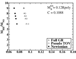
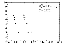
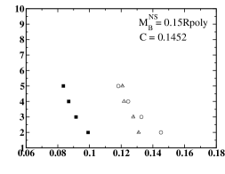
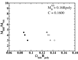
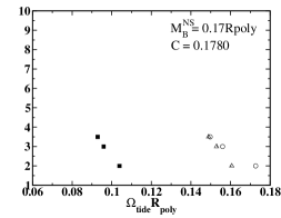
Figure 1: Comparison between Full-GR results from [9] (Full-GR), results obtained with the Newtonian ellipsoidal model of [10] (Newtonian) and results from our improved ellipsoidal model (Pseudo TOV). Each graph shows the mass ratio (Eq. (29)) versus the tidal disruption limit calculated as in Eq. (30). In all cases the neutron star EOS is an $n=1,\kappa=1$ polytrope. The compactness $C$ indicated in each panel refers to the Full-GR and to our models.

3.2 BH-NS Equilibrium Sequences and Tidal Disruption Limits

Having tested the validity of our approach, we employ it to study different possible BH-NS binary configurations, determining the quasi-equilibrium sequences and the tidal disruption radius $r_{tide}$ for equatorial circular orbits. We describe the fluid forming the NS with two different EOS proposed in recent years by the nuclear physics community, which we call APR2 and BALBN1H1.

• The Akmal-Pandharipande-Ravenhall (APR2) hadronic EOS [21] describes matter consisting of neutrons, protons, electrons and muons in weak equilibrium; it is obtained within nuclear many-body theory using a variational approach to the Shrödinger equation; its microscopic input is based on the Argonne $v_{18}$ potential for nucleon-nucleon interactions [22] — which is calibrated to deuteron properties and vacuum nucleon-nucleon phase shifts for laboratory energies $E_{lab}$ up to $350\,$MeV — and on the Urbana IX ($UIX$) three-body potential [23]; relativistic corrections to both potentials are included [24] (which yields $v_{18}+\delta v+UIX^{*}$)

• The Balberg-Gal (BALBN1H1) EOS [25] describes matter consisting of neutrons, protons, electrons, muons and hyperons ($\Sigma$, $\Lambda$ and $\Xi$) in equilibrium. Assuming the mean field approximation, an effective potential is employed, whose parameters are tuned in order to reproduce the properties of nuclei and hypernuclei according to high energy experiments. This EOS is a generalization of the Lattimer-Swesty EOS, which does not include hyperons.

APR2 is much stiffer than BALBN1H1 and, in terms of stiffness, most modern EOS fall in between the two equations of state we choose.

We consider several values of the mass ratio $q=M_{BH}/M_{NS}$, ranging from $5$ to $50$, and three different values of the black hole spin: $a=0$, $a=0.5M_{BH}$ and $a=0.99M_{BH}$.

In order to understand which sequences are possible candidates to be the engine of a SGRB, we compare the tidal disruption orbital separations $r_{tide}$ with $r_{ISCO}$. In the Schwarzschild case, we determine the location of the ISCO through the analytic fit given in [9], where the effects of the finite mass ratio and of the stellar compactness are taken into account:

$$r_{ISCO}=M_{BH}\frac{1+q^{-1}}{6^{-3/2}\left(1-0.444q^{-1/4}(1-3.54C^{1/3})\right)}.$$ (32)

Note that according to this equation the values of $r_{ISCO}/M_{BH}$ we give for $a=0$ in Figure 2 depend on the mass ratio $q$.

Since no such fit exists for the Kerr BH-NS binaries, when $a\neq 0$ we estimate the ISCO by using the formulae derived in [26] for a point mass in the gravitational field of a Kerr BH:

$$r_{ISCO}=M_{BH}\{3+Z_{2}\mp[(3-Z_{1})(3+Z_{1}+2Z_{2})]^{1/2}\}$$ (33)

$$Z_{1}=1+(1-a^{2}/M_{BH}^{2})^{1/3}[(1+a/M_{BH})^{1/3}+(1-a/M_{BH})^{1/3}]$$

$$Z_{2}=(3a^{2}/M_{BH}^{2}+Z_{1}^{2})^{1/2},$$

where the upper sign holds for corotating orbits and the lower sign for counterotating orbits. Note that according to these equations the values that $r_{ISCO}/M_{BH}$ assumes for $a\neq 0$ do not depend on $q$.

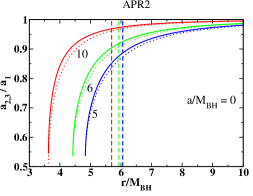
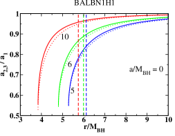
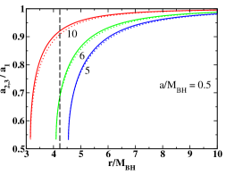
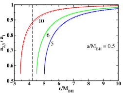
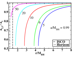
Figure 2: $a_{2}/a_{1}$ (continuous lines) and $a_{3}/a_{1}$ (dotted lines) are plotted as functions of $r/M_{BH}$ for a NS orbiting a black hole. The angular momentum of the BH takes the values $a/M_{BH}=\{0,0.5,0.99\}$ as indicated in each panel. The mass ratio $q=M_{BH}/M_{NS}$ is indicated by the numbers next to each curve, which represent a quasi-equilibrium sequence. $M_{NS}=1.4\,M_{\odot}$ in all graphs: in the left column the star is modeled using APR2 EOS ($R_{NS}=12.84\,$km), in the right column using BALBN1H1 EOS ($R_{NS}=11.53\,$km). The ISCOs are shown by the dashed vertical lines, while the dot-dashed lines in the lower graphs mark the position of the black hole horizon. In the $q=50$ case, the sequence does not terminate with tidal disruption; it stops when $r=a_{1}+R_{BH}^{+}$, where $R_{BH}^{+}$ is the size of the black hole outer horizon at the equatorial plane.

The results of our numerical integrations are displayed in Figure 2, where the ratios $a_{2}/a_{1}$ (continuous lines) and $a_{3}/a_{1}$ (dotted lines) among the NS axes are shown as functions of $r/M_{BH}$; the quasi-equilibrium sequences end when the tidal disruption of the NS is reached (see §2.4). The left panels refer to the EOS APR2, the right ones to BALBN1H1; the upper panels refer to the Schwarzschild case, the middle panels to $a=0.5M_{BH}$, the lower panels to $a=0.99M_{BH}$. The dashed, vertical lines are the locations of the ISCO. In the $a=0.99M_{BH}$ case we also indicate the location of the black hole outer horizon $R_{BH}^{+}$ with a dot-dashed vertical line. From the graphs in Figure 2 we extract the following information.

• In each panel, the larger the mass ratio $q$ is, the closer the NS can get to the BH before being disrupted, i.e. $r_{tide}/M_{BH}$ decreases as $q$ increases. Therefore the conditions of the SGRB mechanism are more likely to be satisfied for low values of $q$.

• If $a=0$ (first row) the star enters the ISCO before being disrupted for all the considered values of $q$, and for both the APR2 and the BALBN1H1 EOS: therefore, SGRBs cannot be ignited. On the other hand, if $a=0.5M_{BH}$ (middle row) the star is disrupted at $r>r_{ISCO}$ for $q\lesssim 5.7$ (APR2 EOS) and $q\lesssim 6.6$ (BALBN1H1 EOS) and the SGRB may take place. If, finally, $a=0.99M_{BH}$ (third row), the star is disrupted at $r>r_{ISCO}$ for $q\lesssim 28$ (APR2 EOS) and $q\lesssim 33$ (BALBN1H1 EOS) and, again, the SGRB may take place.

  We note that as the the black hole spin increases, both $r_{tide}/M_{BH}$ and $r_{ISCO}/M_{BH}$ decrease; however, $r_{ISCO}/M_{BH}$ decreases more rapidly than $r_{tide}/M_{BH}$, and consequently for a given mass ratio $q$, chances to develop an SGRB are higher if the black holes rotates faster. Thus, in general the conditions for the SGRB mechanism proposed in [2] to take place are favoured for low values of $q$ and high values of $a$.

• Comparing the two graphs in each row, we see that for NSs with a stiffer EOS, $r_{tide}/M_{BH}$ is smaller. This is what one expects, since a star with a stiffer EOS is more compact and thus less deformable: hence a stronger gravitational field is needed to disrupt the star.

• As the value of the BH spin increases, the values of the axes $a_{2}$ (continuous lines) and $a_{3}$ (dotted lines) tend to coincide.

We also note that, if $a=0.99M_{BH}$, for $q\simeq 20$ the star enters the ergosphere ($r=2M$, since $\theta=\pi/2$) before disruption.

4 Conclusions

In this paper we have studied the effects of a Kerr BH tidal field on a NS; we have focused on determining the orbital separation at which the NS is tidally disrupted ($r_{tide}$) and the star quasi-equilibrium sequence for several BH-NS binaries. Our work is based on the affine model, which we have improved with respect to previous works, by describing the NS self-gravity with an effective relativistic scalar potential (Eqs. (23) and (24)), and by using more realistic equations of state for the NS matter. This approach has the advantage of allowing a quick computation of $r_{tide}$ and of the quasi-equilibrium sequences for any value of the binary mass ratio $q$ and of the BH spin parameter $a$.

A comparison of the results obtained using our approach for NS disruption with Full-GR results, which are available in the case of non-rotating BHs and polytropic NSs, shows an excellent agreement up to small values of $q$ (which depend on the NS compactness), beyond which our model starts to underestimate $r_{tide}$; this happens because we assume that the centre of mass of the star moves on along a BH geodesic, a condition which is better satisfied for larger mass ratios. Our model agrees with relativistic calculations much better than ellipsoidal models in which the neutron star self-gravity is treated at a Newtonian level.

Given the very good results of this test, we have determined the quasi-equilibrium sequences and the tidal disruption radii of several BH-NS binaries in order to evaluate with our model the role played by (1) the BH spin parameter $a$ and (2) the equation of state of the NS fluid. We found that the soft gamma-ray burst scenario is favoured by low values of the mass ratio $q$ and high values of the BH spin parameter $a$. In addition, the higher the BH spin parameter is, the more the values of the NS axes $a_{2}$ and $a_{3}$ (i.e. the principal axes which do not point at the BH) tend to coincide.

In quantitative terms we have shown that, for the stiffer equation of state APR2 a SGRB may occur if $q\lesssim 28$ when $a=0.99\,M_{BH}$ or if $q\lesssim 5.7$ when $a=0.5\,M_{BH}$. For the softer equation of state BALBN1H1 a SGRB may develop if $q\lesssim 33$ when $a=0.99\,M_{BH}$ or if $q\lesssim 6.6$ when $a=0.5\,M_{BH}$.

As a future development of our work, we intend to study the dynamical behaviour of BH-NS binaries and to determine the gravitational radiation emitted in the late phases of their inspiral. This means taking into account tidal interaction corrections to the orbital dynamics and to the gravitational waveform, and thus will require the inclusion in our model of a precise treatment of the orbit. Moreover we would like to improve the results of our model for low values of the mass ratio $q$.

Appendix A Effective General Relativistic Gravitational Potential

In a Newtonian context, the gravitational potential of a non-rotating star at equilibrium is governed by the Poisson equation and the hydrostatic equilibrium equation, i.e.

$$\Delta\Phi_{Newt} = 4\pi\rho$$ (34)

$$\frac{d\Phi_{Newt}}{dr} = -\frac{1}{\rho}\frac{dP}{dr},$$

and the system is closed by choosing an equation of state.

In General Relativity, the equilibrium configuration of a spherical distribution of fluid is determined by the Tolman-Oppenheimer-Volkoff (TOV) equations of hydrostatic equilibrium

$$\frac{dm(r)}{dr} = 4\pi r^{2}\epsilon(r)$$ (35)

$$\frac{d\nu(r)}{dr} = 2\frac{m(r)+4\pi r^{3}P(r)}{r(r-2m(r))}$$

$$\frac{dP(r)}{dr} = -\frac{(P(r)+\epsilon(r))}{2}\frac{\nu(r)}{dr}$$

where $m(r)$ is the gravitational mass enclosed within a radius $r$; also this system must be closed by choosing an equation of state. In order to define the effective relativistic or pseudo-relativistic scalar potential we use in this work, as in [15]-[17] we “mix together” equations (34)-(35), i.e. we describe the equilibrium configurations using the following equations

$$\frac{dP}{dr} = -\frac{(\epsilon+P)(m_{TOV}+4\pi r^{3}P)}{r(r-2m_{TOV})}$$ (36)

$$\frac{dm_{TOV}}{dr} = 4\pi\epsilon r^{2}$$

$$\frac{d\Phi_{TOV}}{dr} = -\frac{1}{\rho}\frac{dP}{dr}$$

where the first two are the first two TOV equations (35), and the last is the second Newtonian equation (34). The potential $\Phi_{TOV}(r)$ obtained by integrating equations (36) is then used in the self-gravity tensor

$$\hat{V}_{ij}=-\int dM\partial_{i}(\Phi)r_{j}$$ (37)

which is needed to find $\hat{V}=\textrm{Tr}(\hat{V}_{ij})$ used in the self-gravity potential (20).

Appendix B Tidal Disruption Data from Different Models

In Table 1, we provide the data plotted in Figure 1. A polytropic EOS with $n=1$ and $\kappa=1$ is used to model the star. Each data set corresponds to one of the panels in Figure 1, which is identified by the row indicating the NS compactness $C$ and its gravitational mass normalised with respect to the polytropic length scale $R_{poly}=\kappa^{n/2}$. The first column gives the mass ratio $q$. The remaining three columns are the orbital angular frequencies at tidal disruption, normalised with respect to $R_{poly}/10$, resulting from calculations performed with the three binary models considered: “Full GR” indicates data extracted from Figure 11 of [9], “Pseudo GR” data obtained with our model and “Newtonian” data obtained with the model of [10] in which the NS self-gravity is Newtonian. We remind the reader that the BH is always non rotating (the BHs in [9] actually have a small residual angular momentum, see the reference for further details).

$C=0.1088$		$M_{NS}/R_{poly}=0.1136$
$q$	Full GR	Pseudo GR	Newtonian
$9$	$0.88$	$0.88$	$0.70$
$8$	$0.89$	$0.91$	$0.71$
$7.5$	$0.90$	$0.92$	$0.72$
$7$	$0.91$	$0.94$	$0.74$
$6$	$0.93$	$0.96$	$0.75$
$C=0.1201$		$M_{NS}/R_{poly}=0.1223$
$7$	$0.97$	$0.99$	$0.75$
$6.5$	$0.99$	$1.00$	$0.76$
$6$	$1.00$	$1.02$	$0.77$
$5$	$1.04$	$1.05$	$0.80$
$3$	$1.08$	$1.16$	$0.87$
$C=0.1321$		$M_{NS}/R_{poly}=0.1310$
$6$	$1.06$	$1.07$	$0.79$
$5$	$1.08$	$1.11$	$0.82$
$4$	$1.11$	$1.17$	$0.85$
$3$	$1.16$	$1.24$	$0.89$
$C=0.1452$		$M_{NS}/R_{poly}=0.1395$
$5$	$1.21$	$1.18$	$0.84$
$4$	$1.22$	$1.24$	$0.87$
$3$	$1.28$	$1.33$	$0.92$
$2$	$1.31$	$1.45$	$0.99$
$1$	$1.37$	$1.72$	$1.17$
$C=0.1600$		$M_{NS}/R_{poly}=0.1478$
$4.5$	$1.28$	$1.29$	$0.87$
$4$	$1.31$	$1.33$	$0.89$
$3$	$1.35$	$1.43$	$0.94$
$C=0.1780$		$M_{NS}/R_{poly}=0.1560$
$3.5$	$1.49$	$1.50$	$0.93$
$3$	$1.53$	$1.56$	$0.96$
$2$	$1.61$	$1.73$	$1.04$

Table 1: Data plotted in Figure 1: each subtable corresponds to a panel of the figure, which is identified by the stellar compactness $C$ and the gravitational mass normalised with respect to $R_{poly}=\kappa^{n/2}$. The mass ratio $q$ is given in the first column, while the orbital angular frequency calculated at the tidal disruption limit resulting from each model considered here — Full-GR, Pseudo GR, Newtonian — is displayed in the form $\Omega_{tide}R_{poly}/10$ in the other three columns. See the text of the appendix for more details.

References

References

-
[1]
Acernese F et al(VIRGO collaboration) 2007 Class. Quantum Grav.24
381
Abbott B et al(LIGO Scientific Collaboration) 2008 Phys. Rev.D 77 062002
Lück H et al(GEO600 Collaboration) 2006 Class. Quantum Grav.23 71
Ando M et al(TAMA Collaboration) 2005 Class. Quantum Grav.22 881
Heinzel G et al2006 Class. Quantum Grav.23 119
Kawamura S et al(DECIGO Collaboration) 2006 Class. Quantum Grav.23 125 - [2] Narayan R, Paczynski B and Piran T 1992 Astrophys. J. Lett. 395 83
- [3] Fryer C K, Woosley S E and Hartmann D H 1999 Astrophys. J. 526 152
- [4] Lee W H and Ramirez-Ruiz E 2007 New J. Phys.9 17
- [5] Blanchet L 2006 Living Reviews in Relativity 9 4
- [6] Berti E, Iyer S and Will C M 2008 Phys. Rev.D 77 024019
- [7] Casalvieri C, Ferrari V and Stavridis A 2006 Mon. Not. R. Astron. Soc. 365 929
-
[8]
Shibata M and Uryū K 2007 Class. Quantum Grav.24 125
Shibata M and Taniguchi K 2008 Phys. Rev.D 77 084015
Yamamoto T, Shibata M and Taniguchi K 2008 Phys. Rev.D 78 064054
Duez M D et al2008 Phys. Rev.D 78 104015
Tsokaros A A and Uryū K 2007 Phys. Rev.D 75 044026
Löffler F, Rezzolla L and Ansorg M 2006 Phys. Rev.D 74 104018
Sopuerta C F, Sperhake U and Laguna P 2006 Class. Quantum Grav.23 579
Grandclement P 2006 Phys. Rev.D 74 124002
Taniguchi K et al2005 Phys. Rev.D 044008
Taniguchi K et al2007 Phys. Rev.D 75 084005
Faber J A et al2006 Astrophys. J. Lett. 641 93
Faber J A et al2006 Phys. Rev.D 73 024012
Etienne Z B et al2008 Phys. Rev.D 77 084002
Etienne Z B et al2008 Preprint 0812.2245 - [9] Taniguchi K et al2008 Phys. Rev.D 77 044003
- [10] Wiggins P and Lai D 2000 Astrophys. J. 532 530
- [11] Carter B and Luminet J P 1985 Mon. Not. R. Astron. Soc. 212 23
- [12] Luminet J P and Marck J A 1985 Mon. Not. R. Astron. Soc. 212 57
- [13] Chandrasekhar S 1969 Ellipsoidal Figures of Equilibrium (The Silliman Foundation Lectures, New Haven: Yale University Press)
- [14] Lattimer J M and Schramm D N 1976 Astrophys. J. 210 549
- [15] Rampp M and Janka H T 2002 Astron. Astrophys. 396 361
- [16] Liebendörfer M et al2005 Astrophys. J. 620 840
- [17] Marek A et al2006 Astron. Astrophys. 445 273
-
[18]
Lai D, Rasio F A and Shapiro S L 1993 Astrophys. J., Suppl.
88 205
Lai D, Rasio F A and Shapiro S L 1994 Astrophys. J. 437 742 -
[19]
Kochanek C S 1992 Astrophys. J. 398 234
Bildsten L and Cutler C 1992 Astrophys. J. 400 175 - [20] Lattimer J M and Prakash M 2007 Phys. Rep. 442 109
-
[21]
Akmal A and Pandharipande V R 1997 Phys. Rev.C 56 2261
Akmal A and Pandharipande V R and Ravenhall D G 1998 Phys. Rev.C 58 1804 - [22] Wiringa R B, Stoks V G J and Schiavilla R 1995 Phys. Rev.C 51 38
- [23] Pudliner B S et al1997 Phys. Rev.C 56 1720
- [24] Forest J L, Pandharipande V R and Friar J L 1995 Phys. Rev.C 52 568
- [25] Balberg S and Gal A 1997 Nucl. Phys.A 625 435
- [26] Bardeen J M, Press W H and Teukolsky S A 1972 Astrophys. J. 178 347