Binary black holes in circular orbits. I. A global spacetime approach

Abstract

We present a new approach to the problem of binary black holes in the pre-coalescence stage, i.e. when the notion of orbit has still some meaning. Contrary to previous numerical treatments which are based on the initial value formulation of general relativity on a (3-dimensional) spacelike hypersurface, our approach deals with the full (4-dimensional) spacetime. This permits a rigorous definition of the orbital angular velocity. Neglecting the gravitational radiation reaction, we assume that the black holes move on closed circular orbits, which amounts to endowing the spacetime with a helical Killing vector. We discuss the choice of the spacetime manifold, the desired properties of the spacetime metric, as well as the choice of the rotation state for the black holes. As a simplifying assumption, the space 3-metric is approximated by a conformally flat one. The problem is then reduced to solving five of the ten Einstein equations, which are derived here, as well as the boundary conditions on the black hole surfaces and at spatial infinity. We exhibit the remaining five Einstein equations and propose to use them to evaluate the error induced by the conformal flatness approximation. The orbital angular velocity of the system is computed through a requirement which reduces to the classical virial theorem at the Newtonian limit.

We dedicate this work to the memory of our friend and collaborator Jean-Alain Marck.

I Background and motivation

Binary black holes have been the subject of numerous studies in the past two decades, both from the analytical and numerical point of view. These studies are motivated by the fact that the coalescence of two black holes is expected to be one of the strongest sources of gravitational waves detectable by the interferometric detectors LIGO, GEO600, TAMA300 and VIRGO, currently coming on-line [1].

From the analytical point of view, the most recent works are based on the post-Newtonian formalism (see e.g. Ref. [2] for a review) or on the effective one-body approach developed by Buonanno and Damour [3, 4, 5]. In these works, the black holes are treated as point mass particles, which is a very good approximation when the black holes are far apart. For closer configurations, one may turn instead to some numerical approach. The numerical studies can be divided in two classes: (i) the initial value problem for two black holes (see Ref. [7] for a review) and (ii) the time evolution of the initial data (see Ref. [8] for a review and Refs. [9, 10, 11] for recent results). One of the major problems in this respect is to get physically relevant initial data. Indeed, initial data representing two black holes have been obtained long ago by Misner [12] and Lindquist [13], as well as Brill and Lindquist [14] (a modern discussion of these solutions can be found in Ref. [15] or Appendices A and B of Ref. [16]). However these solutions correspond to two momentarily static black holes and are therefore far from representing some stage in the evolution of an isolated binary black hole in our universe.

Based on the seminal work of Bowen and York [17], Kulkarni, Shepley and York [18] have described a procedure to get initial data representing binary black hole with arbitrary positions, masses, spins and momenta. This procedure, known as conformal imaging, has been used by Cook and other authors [19, 20, 21, 22, 23] to numerically construct 3-dimensional spacelike hypersurfaces representing these initial data. These solutions constitute some generalization to the non-static regime of the Misner-Lindquist solution [12, 13], the spacelike hypersurface having the same topology: two isometric asymptotically-flat sheets connected by two Einstein-Rosen bridges. Also based on the Bowen and York’s work [17], another approach, the so-called puncture method, has been undertaken by Brandt and Brügmann [24] and used recently by Baumgarte [25]. The resulting solutions also have arbitrary positions, masses, spins and momenta but their topology is different from that of the conformal-imaging approach: the spacelike hypersurface has now three asymptotically-flat sheets, which are not isometric. These three sheets are connected among themselves by two Einstein-Rosen bridges; one of the sheets contains two throats and is supposed to represent our universe. These solutions hence constitute some generalization to the non-static case of the Brill-Lindquist solution [14]. Both the conformal-imaging and the puncture approaches assume that the metric of the spacelike hypersurface is conformally flat. A third approach to the problem relaxes this assumption; it has been developed recently by Matzner, Maroronetti and collaborators [26, 27, 28]. These authors use a linear combination of two boosted Kerr-Schild metrics as the conformal 3-metric in York’s treatment of initial conditions [29].

The main drawback of the three approaches described above is that they contain freely specifiable parameters, related to the values of positions, momenta and spins of the black holes, and it is difficult to figure out which parameters correspond to a physical configuration. In particular, it is not obvious at all how to select, among all these configurations, those that correspond to binary black holes on closed circular orbits. Of course, the circular orbits are approximate representations of the exact orbital motion, which is inspiralling due to the loss of energy and angular momentum via gravitational radiation. However in the regime where the radiation reaction time scale is much longer than the orbital time scale, i.e. before the last stable orbit, we expect that the binary system can be approximated by a sequence of tighter and tighter circular orbits. Note that the gravitational radiation reaction makes initially elliptic orbits become circular [30]. It is thus legitimate to search for such orbits. This problem has been addressed by Cook [21] and Pfeiffer et al. [22] within the conformal-imaging approach and by Baumgarte [25] within the puncture approach (see e.g. [31] for a review of these computations). Although they differ in the topology of the spacelike hypersurface (two-sheeted for [21, 22] against three-sheeted for [25]), both sets of studies rely on the effective-potential method proposed by Cook [21]. This method amounts to defining the binding energy by a somewhat ad-hoc formula, and to define the angular velocity of a circular orbit by minimizing the binding energy with respect to the angular momentum at fixed total energy and separation. This method can be criticized on the following ground: the only well defined global quantities on an asymptotically flat spacelike hypersurface are the ADM total mass $M$ and ADM total linear momentum. The latter can be chosen to be zero without any loss of generality. With some restrictions on the asymptotic gauge, the total angular momentum $J$ can also be defined [32]. Defining the binding energy would require the notion of individual mass for each hole, let say $M_{1}$ and $M_{2}$, in order to set $E_{\rm bind}=M-M_{1}-M_{2}$. However there does not exist any unique definition of the individual masses $M_{1}$ and $M_{2}$ for a binary black hole. In Refs. [21, 22, 25] the authors define $M_{1}$ and $M_{2}$ via the formula which relates the mass of a Kerr black hole to its horizon area and its angular momentum. However such a formula is strictly demonstrated only for a isolated rotating black hole (Kerr spacetime). In particular, it does not take into account any tidal effect.

Our approach for finding circular orbits of binary black holes is very different: instead of considering 3-dimensional spacelike hypersurfaces, we adopt from the very beginning a 4-dimensional point of view, i.e. we consider a full spacetime containing two moving black holes. Of course, in order to make the problem tractable, we introduce some approximations, the most significant being the assumption of strictly circular orbits, which amounts to endowing our spacetime with a Killing vector field (helical symmetry). An interesting pay-off is that the orbital angular velocity $\Omega$ can be unambiguously defined as the rotation rate of the Killing field with respect to some asymptotically inertial observers. This definition does not suffer from the ambiguity of the 3-dimensional approaches and is made possible only because we have re-introduced time in the problem.

The presentation of this new approach is organized as follows. We set up the problem in Sec. II, starting from the explicit construction of the spacetime manifold, introducing a metric, as well as a corresponding isometry on it, and finally imposing the helical symmetry. The Einstein equations are then considered in Sec. III, first in their general form and then after the assumption of a conformally flat 3-metric. Global quantities such as the ADM mass and the total angular momentum are discussed in this section, as well as the virial prescription for the orbital velocity. Section IV deals with the asymptotic behavior of the shift vector and the extrinsic curvature tensor and discusses the connection between helical symmetry and asymptotic flatness. Finally Sec. V contains the concluding remarks.

II Formulation

A Spacetime manifold

1 Construction

We consider the spacetime to be a differentiable manifold $\cal M$ with the topology of the real line ${\mathbb{R}}$ times the Misner-Lindquist manifold [12, 13]. More precisely, for any couple of positive numbers $(a_{1},a_{2})$ and any couple of real numbers $(x_{1},x_{2})$ such that $|x_{1}-x_{2}|>a_{1}+a_{2}$, let us consider the subset of ${{\mathbb{R}}^{3}}$ obtained by removing the interior of balls of radius $a_{1}$ and $a_{2}$ and center $x=x_{1}$ and $x=x_{2}$:

$${\cal E}:=\left\{(x,y,z)\in{{\mathbb{R}}^{3}},(x-x_{1})^{2}+y^{2}+z^{2}\geq a_{1}^{2}\ \mbox{and}\ (x-x_{2})^{2}+y^{2}+z^{2}\geq a_{2}^{2}\right\}\ .$$ (1)

Let us call $S_{1}$ and $S_{2}$ the 2-spheres defining the “inner” boundaries of $\cal E$:

$$S_{1}:=\left\{(x,y,z)\in{\mathbb{R}}^{3},(x-x_{1})^{2}+y^{2}+z^{2}=a_{1}^{2}\right\}\ ,$$ (2)

$$S_{2}:=\left\{(x,y,z)\in{\mathbb{R}}^{3},(x-x_{2})^{2}+y^{2}+z^{2}=a_{2}^{2}\right\}\ .$$ (3)

Let us consider two copies ${\cal E}_{\rm I}$ and ${\cal E}_{\rm II}$ of $\cal E$ and define ${\cal M}_{\rm I}:={\mathbb{R}}\times{\cal E}_{\rm I}$ and ${\cal M}_{\rm II}:={\mathbb{R}}\times{\cal E}_{\rm II}$. The spacetime manifold $\cal M$ is be then defined as the union ${\cal M}_{\rm I}\cup{\cal M}_{\rm II}$ with both $S_{1}$ and $S_{2}$ of each copy identified (see Fig. 1). The reader is referred to Sect. IV of Ref. [12] or Sect. II of Ref. [13] for a precise construction of the manifold structure in the vicinity of $S_{1}$ and $S_{2}$. The part ${\cal M}_{\rm I}$ of $\cal M$ will be designed hereafter as the upper space and the part ${\cal M}_{\rm II}$ as the lower space. The boundaries ${\cal S}_{1}:={\mathbb{R}}\times S_{1}$ and ${\cal S}_{2}:={\mathbb{R}}\times S_{2}$ between ${\cal M}_{\rm I}$ and ${\cal M}_{\rm II}$ are called respectively throat 1 and throat 2.

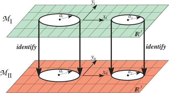
FIG. 1.: Construction of the spacetime manifold.

Hereafter we label by $(t,x_{\rm I},y_{\rm I},z_{\rm I})$ the points of ${\cal M}_{\rm I}$ considered as a part of ${\mathbb{R}}\times{\mathbb{R}}^{3}$ (${\cal E}_{\rm I}$ being a part of ${\mathbb{R}}^{3}$), and by $(t,x_{\rm II},y_{\rm II},z_{\rm II})$ the points of ${\cal M}_{\rm II}$ considered as a part of ${\mathbb{R}}\times{\mathbb{R}}^{3}$. The corresponding two charts will be called the canonical coordinate systems. These two charts cover $\cal M$ minus the two throats. The whole manifold $\cal M$ can be covered entirely by a single coordinate system:

$$\begin{array}[]{cccl}C_{1}:&{\cal M}&\longrightarrow&{\mathbb{R}}^{4}\\ &P&\longmapsto&\left\{\begin{array}[]{ll}(t,x_{\rm I},y_{\rm I},z_{\rm I})&{\rm if\ }P\in{\cal M}_{\rm I}\\ {\cal I}_{1}(t,x_{\rm II},y_{\rm II},z_{\rm II})&{\rm if\ }P\in{\cal M}_{\rm II}\end{array}\right.\end{array}\ ,$$ (4)

where ${\cal I}_{1}:{\mathbb{R}}^{4}\mapsto{\mathbb{R}}^{4}$ denotes the inversion through the 2-sphere $S_{1}$ :

$${\cal I}_{1}(t,x,y,z)=\left(t,\ {a_{1}^{2}(x-x_{1})\over(x-x_{1})^{2}+y^{2}+z^{2}}+x_{1},\ {a_{1}^{2}y\over(x-x_{1})^{2}+y^{2}+z^{2}},\ {a_{1}^{2}z\over(x-x_{1})^{2}+y^{2}+z^{2}}\right)\ .$$ (5)

In a similar way, one can introduce the coordinate system $C_{2}$ associated with throat 2.

In the coordinate system $C_{1}$ or $C_{2}$, the throats are not located at constant coordinate values. Therefore, it is more convenient to introduce instead the polar coordinate system $(t,r_{1},\theta_{1},\varphi_{1})$ centered on throat 1, as follows:

$$\mbox{for}\ P\in{\cal M}_{\rm I},\quad\left\{\begin{array}[]{l}x_{\rm I}=r_{1}\sin\theta_{1}\cos\varphi_{1}+x_{1}\\ y_{\rm I}=r_{1}\sin\theta_{1}\sin\varphi_{1}\\ z_{\rm I}=r_{1}\cos\theta_{1}\end{array}\right.\qquad(a_{1}\leq r_{1}<+\infty)$$ (6)

and

$$\mbox{for}\ P\in{\cal M}_{\rm II},\quad\left\{\begin{array}[]{l}x_{\rm II}={a_{1}^{2}\over r_{1}}\sin\theta_{1}\cos\varphi_{1}+x_{1}\\ y_{\rm II}={a_{1}^{2}\over r_{1}}\sin\theta_{1}\sin\varphi_{1}\\ z_{\rm II}={a_{1}^{2}\over r_{1}}\cos\theta_{1}\end{array}\right.\qquad(0<r_{1}\leq a_{1})\ .$$ (7)

The throat 1 corresponds to $r_{1}=a_{1}$. The polar coordinate system $(t,r_{2},\theta_{2},\varphi_{2})$ centered on throat 2 is introduced similarly. Note that any of the two coordinate systems $(t,r_{1},\theta_{1},\varphi_{1})$ and $(t,r_{2},\theta_{2},\varphi_{2})$ covers the whole spacetime manifold $\cal M$. For the $(t,r_{1},\theta_{1},\varphi_{1})$ system, $\cal M_{\rm I}$ corresponds to $a_{1}\leq r_{1}<+\infty$ and $\cal M_{\rm II}$ to $0<r_{1}\leq a_{1}$. Similarly, for $(t,r_{2},\theta_{2},\varphi_{2})$ system, $\cal M_{\rm I}$ corresponds to $a_{2}\leq r_{2}<+\infty$ and $\cal M_{\rm II}$ to $0<r_{2}\leq a_{2}$ (see Fig. 2).

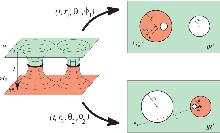
FIG. 2.: Coordinate systems $(t,r_{1},\theta_{1},\varphi_{1})$ and $(t,r_{2},\theta_{2},\varphi_{2})$ on the spacetime manifold $\cal M$. Shown here is a $t={\rm const}$ section of $\cal M$, with the dimension in the $\theta$ direction suppressed, leaving only $(r_{1},\varphi_{1})$ or $(r_{2},\varphi_{2})$.

2 Canonical mapping

From the very construction of $\cal M$, we have at our disposal the canonical mapping (see Fig. 1)

$$\begin{array}[]{lccc}I:&{\cal M}_{\rm I}&\longrightarrow&{\cal M}_{\rm II}\\ &(t,x_{\rm I},y_{\rm I},z_{\rm I})&\longmapsto&(t=t,x_{\rm II}=x_{\rm I},y_{\rm II}=y_{\rm I},z_{\rm II}=z_{\rm I})\end{array}$$ (8)

Note that in terms of the $(t,r_{1},\theta_{1},\varphi_{1})$ coordinate system, this map can be written as an inversion through the sphere $r_{1}=a_{1}$ (see Fig. 2):

$$I(t,r_{1},\theta_{1},\varphi_{1})=\left(t,{a_{1}^{2}\over r_{1}},\theta_{1},\varphi_{1}\right)\ .$$ (9)

In terms of the $(t,r_{2},\theta_{2},\varphi_{2})$ coordinate system, it looks like an inversion as well:

$$I(t,r_{2},\theta_{2},\varphi_{2})=\left(t,{a_{2}^{2}\over r_{2}},\theta_{2},\varphi_{2}\right)\ .$$ (10)

Let $(x^{\alpha})$ be a coordinate system on ${\cal M}_{\rm I}$ [for instance $(x^{\alpha})=(t,x_{\rm I},y_{\rm I},z_{\rm I})$, $(x^{\alpha})=(t,r_{1},\theta_{1},\varphi_{1})$ or $(x^{\alpha})=(t,r_{2},\theta_{2},\varphi_{2})$] and $(y^{\mu})$ be a coordinate system on ${\cal M}_{\rm II}$ [for instance $(y^{\mu})=(t,x_{\rm II},y_{\rm II},z_{\rm II})$, $(y^{\mu})=(t,r_{1},\theta_{1},\varphi_{1})$ or $(y^{\mu})=(t,r_{2},\theta_{2},\varphi_{2})$]. The map $I$ is fully characterized by its components $I^{\mu}$ with respect to the coordinates $(x^{\alpha})$ and $(y^{\mu})$: the image $I(P)$ of a point $P\in{\cal M}_{\rm I}$ with coordinates $(x^{0},x^{1},x^{2},x^{3})$ has the coordinates

$$y^{\mu}=I^{\mu}(x^{0},x^{1},x^{2},x^{3})\ .$$ (11)

Let us now examine the action of the map $I$ on various fields on $\cal M$. If $f$ is a scalar field on ${\cal M}_{\rm II}$, $I$ induces a scalar field on ${\cal M}_{\rm I}$ through

$$I_{*}f:=f\circ I\ ,$$ (12)

i.e.

$$I_{*}f[P]=f[I(P)]\ ,$$ (13)

for any point $P$ of ${\cal M}_{\rm I}$.

Also $I$ maps any vector field v on ${\cal M}_{\rm I}$ to a vector field $I_{*}\mbox{\ssg{v}}$ on ${\cal M}_{\rm II}$ through

$$I_{*}\mbox{\ssg{v}}(f):=\mbox{\ssg{v}}(I_{*}f)\ ,$$ (14)

for any scalar field $f$ on ${\cal M}_{\rm II}$. If vectors are represented by their components with respect to the coordinate bases $\partial/\partial x^{\alpha}$ and $\partial/\partial y^{\mu}$, one has

$$I_{*}\mbox{\ssg{v}}(f)=(I_{*}\mbox{\ssg{v}})^{\mu}{\partial f\over\partial y^{\mu}}$$ (15)

and, according to definitions (14) and (12),

$$I_{*}\mbox{\ssg{v}}(f)=v^{\alpha}{\partial\over\partial x^{\alpha}}f\left(I^{\mu}(x^{\beta})\right)=v^{\alpha}{\partial f\over\partial y^{\mu}}{\partial I^{\mu}\over\partial x^{\alpha}}\ .$$ (16)

Hence the matrix of the mapping $I_{*}$ between vectors on ${\cal M}_{\rm I}$ and vectors on ${\cal M}_{\rm II}$ is given by the Jacobian matrix of $I$:

$$(I_{*}\mbox{\ssg{v}})^{\mu}[I(P)]={\partial I^{\mu}\over\partial x^{\alpha}}\,v^{\alpha}[P]\ ,$$ (17)

where $P$ denotes any point of ${\cal M}_{\rm I}$.

The action of $I$ on vectors can be used to define the action of $I$ on 1-forms as follows: $I$ maps any 1-form ${\omega}$ on ${\cal M}_{\rm II}$ to a 1-form $I_{*}\mbox{\boldmath${\omega}$}$ on ${\cal M}_{\rm I}$ through

$$I_{*}\mbox{\boldmath${\omega}$}(\mbox{\ssg{v}}):=\mbox{\boldmath${\omega}$}(I_{*}\mbox{\ssg{v}})\ ,$$ (18)

for any vector field v on ${\cal M}_{\rm I}$. If 1-forms are represented by their components with respect to the coordinate bases $dx^{\alpha}$ and $dy^{\mu}$, one has

$$I_{*}\mbox{\boldmath${\omega}$}(\mbox{\ssg{v}})=(I_{*}\mbox{\boldmath${\omega}$})_{\alpha}dx^{\alpha}(\mbox{\ssg{v}})=(I_{*}\mbox{\boldmath${\omega}$})_{\alpha}v^{\alpha}$$ (19)

and, according to definition (18),

$$I_{*}\mbox{\boldmath${\omega}$}(\mbox{\ssg{v}})=\omega_{\mu}dy^{\mu}(I_{*}\mbox{\ssg{v}})=\omega_{\mu}(I_{*}\mbox{\ssg{v}})^{\mu}=\omega_{\mu}{\partial I^{\mu}\over\partial x^{\alpha}}v^{\alpha}\ ,$$ (20)

where the third equality arises from Eq. (17). Comparing Eqs. (19) and (20) leads to

$$(I_{*}\mbox{\boldmath${\omega}$})_{\alpha}[P]={\partial I^{\mu}\over\partial x^{\alpha}}\,\omega_{\mu}[I(P)]$$ (21)

at any point $P$ in ${\cal M}_{\rm I}$.

Similarly, the action of $I$ on bilinear forms can be defined as follows: $I$ associates any bilinear form T on ${\cal M}_{\rm II}$ to a bilinear form $I_{*}\mbox{\ssg{T}}$ on ${\cal M}_{\rm I}$ according to

$$I_{*}\mbox{\ssg{T}}(\mbox{\ssg{v}},\mbox{\ssg{w}}):=\mbox{\ssg{T}}(I_{*}\mbox{\ssg{v}},I_{*}\mbox{\ssg{w}})\ .$$ (22)

One can show easily that in terms of the components with respect to the coordinate bases $\mbox{\ssg{d}}x^{\alpha}\otimes\mbox{\ssg{d}}x^{\beta}$ and $\mbox{\ssg{d}}y^{\mu}\otimes\mbox{\ssg{d}}y^{\nu}$,

$$(I_{*}\mbox{\ssg{T}})_{\alpha\beta}[P]={\partial I^{\mu}\over\partial x^{\alpha}}{\partial I^{\nu}\over\partial x^{\beta}}\,T_{\mu\nu}[I(P)]$$ (23)

at any point $P$ in ${\cal M}_{\rm I}$.

B Spacetime metric

1 Properties

We endow $\cal M$ with a Lorentzian metric g with the following properties:

(1) g is asymptotically flat at the ends of ${\cal M}_{\rm I}$ and ${\cal M}_{\rm II}$ :

$$\lim_{x_{\rm I}^{2}+y_{\rm I}^{2}+z_{\rm I}^{2}\rightarrow\infty}\mbox{\ssg{g}} = \mbox{\boldmath${\eta}$}\ ,$$ (24)

$$\lim_{x_{\rm II}^{2}+y_{\rm II}^{2}+z_{\rm II}^{2}\rightarrow\infty}\mbox{\ssg{g}} = \mbox{\boldmath${\eta}$}\ ,$$ (25)

where ${\eta}$ is a flat metric.

(2) the canonical mapping $I$ is an isometry of g:

$$I_{*}\mbox{\ssg{g}}=\mbox{\ssg{g}}\ .$$ (26)

(3) The $t={\rm const}$ sections of $\cal M$ are maximal spacelike hypersurfaces with respect to g.

The assumption (1) is introduced because we consider only isolated systems. Its connection with the quasi-stationarity hypothesis will be discussed in Secs. II C 1 and IV C.

The assumption (2) is motivated by the fact that the Schwarzschild and Kerr spacetimes possess such an isometry. This can be readily seen when using isotropic (quasi-isotropic for Kerr) coordinates instead of the standard Schwarzschild (Boyer-Lindquist) ones. By virtue of Eq. (23), the isometry condition (26) can be expressed in terms of the components of g at any point $P$ in ${\cal M}_{\rm I}$ :

$${\partial I^{\mu}\over\partial x^{\alpha}}{\partial I^{\nu}\over\partial x^{\beta}}\,g_{\mu\nu}[I(P)]=g_{\alpha\beta}[P]\ .$$ (27)

It is also useful to write the isometry condition on the contravariant components of the metric tensor; by means of a generalization of Eq. (17), one gets:

$$g^{\mu\nu}[I(P)]={\partial I^{\mu}\over\partial x^{\alpha}}{\partial I^{\nu}\over\partial x^{\beta}}\,g^{\alpha\beta}[P]\ .$$ (28)

The assumption (3) is motivated by the well-known good properties of maximal slicing [29, 33], among which there is the singularity avoidance.

2 3+1 decomposition

In this article we use the standard 3+1 formalism of general relativity [29], foliating the spacetime by a family of spacelike hypersurfaces. From the very construction of $\cal M$, a natural foliation is by the $t=const$ hypersurfaces $\Sigma_{t}$, where $t$ is the same coordinate as that introduced above. By virtue of assumption (3), this constitutes a maximal slicing of spacetime.

Let us denote by n the future directed unit normal to $\Sigma_{t}$. Being normal to $\Sigma_{t}$, n should be collinear to the gradient of $t$:

$$\mbox{\ssg{n}}=-N\mbox{\boldmath${\nabla}$}t\ ,$$ (29)

where $N$ is the lapse function, which can be seen as a normalization factor such to ensure that $\mbox{\ssg{n}}\cdot\mbox{\ssg{n}}:=\mbox{\ssg{g}}(\mbox{\ssg{n}},\mbox{\ssg{n}})=-1$. Let us now examine the behavior of n under the isometry $I$. By the definition (8), $I$ preserves the hypersurface $\Sigma_{t}$. According to the definition (22), the square of the norm of $I_{*}\mbox{\ssg{n}}$ is

$$\mbox{\ssg{g}}(I_{*}\mbox{\ssg{n}},I_{*}\mbox{\ssg{n}})=(I_{*}\mbox{\ssg{g}})(\mbox{\ssg{n}},\mbox{\ssg{n}})\ .$$ (30)

But thanks to the isometry condition $I_{*}\mbox{\ssg{g}}=\mbox{\ssg{g}}$, the last term in this equation is simply $\mbox{\ssg{n}}\cdot\mbox{\ssg{n}}=-1$. Hence

$$I_{*}\mbox{\ssg{n}}\cdot I_{*}\mbox{\ssg{n}}=-1\ ,$$ (31)

i.e. $I$ preserves the norm of n. Similarly, for any vector v tangent to $\Sigma_{t}$, $I$ preserves the scalar product $\mbox{\ssg{n}}\cdot\mbox{\ssg{v}}=0$, so that $I_{*}\mbox{\ssg{n}}\cdot I_{*}\mbox{\ssg{v}}=0$. But since $\Sigma_{t}$ is globally invariant under $I$, $I_{*}\mbox{\ssg{v}}$ represents any vector tangent to $\Sigma_{t}$, so that $I_{*}\mbox{\ssg{n}}$ is in fact normal to $\Sigma_{t}$. Having the same norm than n, we conclude that

$$I_{*}\mbox{\ssg{n}}=\pm\mbox{\ssg{n}}\ .$$ (32)

Since $t$, considered as a scalar field on $\cal M$, is preserved by $I$, so is its gradient and the relation (29), combined with (32) results then in the following transformation law for the lapse function:

$$I_{*}N=\pm N\ .$$ (33)

In order to understand the significance of the $\pm$ sign in Eqs. (32) and (33), let us consider the case of a single static black hole, i.e. the (extended) Schwarzschild spacetime. Two kinds of maximal slicing of this spacetime are depicted in a Kruskal diagram in Fig. 3, starting from the same initial hypersurface $v=0,\ t=0$. The first one corresponds to a symmetric lapse [sign $+$ in Eqs. (33) and (32)]. The throat is located at $u=0$; the slicing penetrates under the event horizon ($R=2M$), and accumulates on the spacelike hypersurface $R=1.5M$ [34, 35]. The second slicing corresponds to an antisymmetric lapse [sign $-$ in Eqs. (33) and (32)]. In fact, it corresponds to the standard Schwarzschild solution in isotropic coordinates:

$$ds^{2}=-N^{2}dt^{2}+\left(1+{M\over 2r}\right)^{4}\left[dr^{2}+r^{2}(d\theta^{2}+\sin^{2}\theta d\varphi^{2})\right]\ ,$$ (34)

with

$$N={1-M/2r\over 1+M/2r}\ .$$ (35)

This lapse function is clearly antisymmetric under the transformation $I:r\mapsto M^{2}/(4r)$ across the throat located at $r=M/2$. The negative value of the lapse for $r<M/2$ is easily understandable when looking to Fig. 3: while $t$ is running upward on the right part of the diagram (corresponding to ${\cal M}_{\rm I}$), it is running downward on the left part (corresponding to ${\cal M}_{\rm II}$). Since in the Kruskal diagram the future direction is everywhere upward, the lapse should be negative in ${\cal M}_{\rm II}$.

 

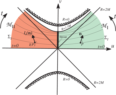
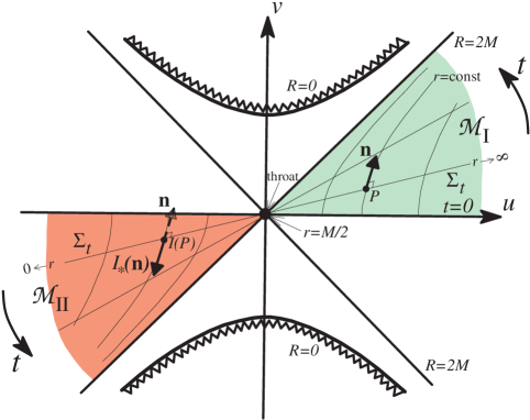
FIG. 3.: Kruskal diagrams showing the slicing of the extended Schwarzschild spacetime by two families of maximal hypersurfaces; left: lapse function symmetric with respect to the isometry $I$; right: lapse function antisymmetric with respect to the isometry $I$. $R$ denotes the standard Schwarzschild radial coordinate and $r$ the isotropic one.

Let us now consider a coordinate system $(x^{i})$ on each $\Sigma_{t}$. For instance, it can be chosen in one of the three coordinate atlas introduced so far: $\{(x_{\rm I},y_{\rm I},z_{\rm I}),\,(x_{\rm II},y_{\rm II},z_{\rm II})\}$, $\{(r_{1},\theta_{1},\varphi_{1})\}$ and $\{(r_{2},\theta_{2},\varphi_{2})\}$. $(t,x^{i})$ constitutes then a coordinate system on $\cal M$. The shift vector ${\beta}$ associated with the coordinates $(t,x^{i})$ is defined by the following orthogonal split of the coordinate basis vector $\partial/\partial t$:

$${\partial\over\partial t}=N\mbox{\ssg{n}}+\mbox{\boldmath${\beta}$}\qquad\mbox{with}\qquad\mbox{\ssg{n}}\cdot\mbox{\boldmath${\beta}$}=0\ .$$ (36)

Since the transformation $I$ is purely spatial $\partial/\partial t$ is preserved by it. By virtue of Eqs. (32) and (33), the product $N\mbox{\ssg{n}}$ is also invariant with respect to $I$. Consequently

$$I_{*}\mbox{\boldmath${\beta}$}=\mbox{\boldmath${\beta}$}\ .$$ (37)

The 3-metric induced by g on the hypersurfaces $\Sigma_{t}$ is

$$\mbox{\boldmath${\gamma}$}=\mbox{\ssg{g}}+\mbox{\ssg{n}}\otimes\mbox{\ssg{n}}\ .$$ (38)

From Eqs. (26) and (32), we obtain immediately that $I$ is also an isometry for the 3-metric ${\gamma}$:

$$I_{*}\mbox{\boldmath${\gamma}$}=\mbox{\boldmath${\gamma}$}\ .$$ (39)

The components of the metric tensor can be expressed in terms of the lapse function and the components of the shift vector and the 3-metric, according to the classical formula

$$g_{\mu\nu}dx^{\mu}dx^{\nu}=-(N^{2}-\beta_{i}\beta^{i})\,dt^{2}+2\beta_{i}\,dt\,dx^{i}+\gamma_{ij}\,dx^{i}\,dx^{j}\ .$$ (40)

The extrinsic curvature tensor K of the hypersurface $\Sigma_{t}$ is given by the Lie derivative of the 3-metric along the flow defined by the normal to $\Sigma_{t}$:

$$\mbox{\ssg{K}}=-{1\over 2}\pounds_{\mbox{\ssg{n}}}\mbox{\boldmath${\gamma}$}\ .$$ (41)

By the symmetry properties (32) and (39), we obtain that

$$I_{*}\mbox{\ssg{K}}=\pm\mbox{\ssg{K}}\ .$$ (42)

3 Explicit isometry conditions in polar coordinates

In what follows, we consider only polar coordinate systems centered on one of the two throats, i.e. either the system $(t,r_{1},\theta_{1},\varphi_{1})$ introduced in Sec. II A 1 or $(t,r_{2},\theta_{2},\varphi_{2})$. For the sake of clarity we will drop the indices $1$ or $2$ on $r$, $\theta$ and $\varphi$. It should be understood that the formulas will be valid for either coordinate system. The Jacobian matrix of $I$ with respect to $(t,r,\theta,\varphi)$ is easily deduced from Eq. (9) or (10):

$${\partial I^{\mu}\over\partial x^{\alpha}}=\mbox{diag}\left(1,\ -{a^{2}\over r^{2}},\ 1,\ 1\right)\ ,$$ (43)

where $a$ denotes either $a_{1}$ or $a_{2}$. From the isometry condition (28) expressed on $g^{tt}$, we get, since $g^{tt}=-1/N^{2}$ :

$$N[I(P)]^{2}=N[P]^{2}\ ,$$ (44)

for any point point $P$ in ${\cal M}_{\rm I}$, i.e. we recover the already established relation (33). From the isometry condition (28) expressed on $g^{ti}$ we get

$$\beta^{r}[I(P)] = -{a^{2}\over r^{2}}\beta^{r}[P]$$ (45)

$$\beta^{\theta}[I(P)] = \beta^{\theta}[P]$$ (46)

$$\beta^{\varphi}[I(P)] = \beta^{\varphi}[P]\ ,$$ (47)

where we have used $g^{ti}=\beta^{i}/N^{2}$ and Eq. (44) to go from $g^{ti}$ to $\beta^{i}$. Again note that we recover the isometry condition (37).

Finally the isometry condition (27) expressed on $g_{ij}=\gamma_{ij}$ results in

$$\gamma_{rr}[P] = {a^{4}\over r^{4}}\gamma_{rr}[I(P)]$$ (48)

$$\gamma_{r\theta}[P] = -{a^{2}\over r^{2}}\gamma_{r\theta}[I(P)]$$ (49)

$$\gamma_{r\varphi}[P] = -{a^{2}\over r^{2}}\gamma_{r\varphi}[I(P)]$$ (50)

$$\gamma_{\theta\theta}[P] = \gamma_{\theta\theta}[I(P)]$$ (51)

$$\gamma_{\theta\varphi}[P] = \gamma_{\theta\varphi}[I(P)]$$ (52)

$$\gamma_{\varphi\varphi}[P] = \gamma_{\varphi\varphi}[I(P)]\ .$$ (53)

Comparing Eqs. (26) and (42), we see that the isometries properties of the components $K_{ij}$ of K are the same as those above for $\gamma_{ij}$, except possibly for an opposite sign.

4 Choice of the isometry sign

As discussed above, the behavior of the foliation with respect to the isometry $I$ involves a $+$ or $-$ sign in the transformation rules of the unit normal [Eq. (32)], lapse function [Eq. (33)] and extrinsic curvature [Eq. (42)]. In this article, we choose the sign to be the minus one. This is motivated by the fact that the maximal slicing with the $+$ sign of the Schwarzschild spacetime (left part of Fig. 3) does not respect the stationarity of the problem, i.e. the Killing vector $\partial/\partial t$ of Schwarzschild geometry does not carry a slice of that foliation into another slice [34] (see also Sec. IV of Ref. [36]). On the contrary, the slicing with the $-$ sign (right part of Fig. 3) respects the stationarity of the problem. It seems to us more appealing to use a slicing which in the case of a single black hole, makes the problem time-independent. We regard the artificial time dependence resulting from the $+$ sign as an unnecessary complication. Beside simplicity, another advantage of the $-$ sign choice is to allow us to test the numerical code by comparison with the standard form of the Schwarzschild or Kerr metric in the special case of a single black hole.

Thus, from now on, we set

$$I_{*}\mbox{\ssg{n}}=-\mbox{\ssg{n}}\ ,$$ (54)

$$I_{*}N=-N\ ,$$ (55)

and

$$I_{*}\mbox{\ssg{K}}=-\mbox{\ssg{K}}\ .$$ (56)

Eq. (55) can be explicited for any point $P$ in ${\cal M}_{\rm I}$:

$$N[I(P)]=-N[P]\ ,$$ (57)

which amounts to choosing the $-$ sign when taking the square root of Eq. (44).

5 Boundary conditions on the throats

An immediate consequence of Eq. (57) is that the lapse function vanishes on the two throats:

$$N|_{{\cal S}_{1}}=0\qquad\mbox{and}\qquad N|_{{\cal S}_{2}}=0\ .$$ (58)

Indeed from the very definition of $I$ [Eq. (8)] and the construction of $\cal M$ by identifications of the two copies of ${\cal S}_{1}$ or ${\cal S}_{2}$, every point $P$ in ${\cal S}_{1}$ or ${\cal S}_{2}$ is a fixed point for $I$. Hence Eq. (57) results in $N[P]=-N[P]$ on ${\cal S}_{1}$ and ${\cal S}_{2}$.

Similarly, Eq. (45) implies that the $r$ component of the shift vector vanishes on the throats:

$$\left.\beta^{r_{1}}\right|_{{\cal S}_{1}}=0\qquad\mbox{and}\qquad\left.\beta^{r_{2}}\right|_{{\cal S}_{2}}=0\ .$$ (59)

Taking the first derivatives of Eqs. (45)-(47), we get the additional following relations on the throats, as a consequence of the isometry of the shift vector:

$$\left.{\partial\beta^{r}\over\partial\theta}\right|_{{\cal S}} = 0$$ (60)

$$\left.{\partial\beta^{r}\over\partial\varphi}\right|_{{\cal S}} = 0$$ (61)

$$\left.{\partial\beta^{\theta}\over\partial r}\right|_{{\cal S}} = 0$$ (62)

$$\left.{\partial\beta^{\varphi}\over\partial r}\right|_{{\cal S}} = 0\ ,$$ (63)

where we have dropped the indices 1 or 2 on $r$, $\theta$, $\varphi$ and $\cal S$. Note that relations (60) and (61) could have been obtained also as consequences of Eq. (59) since the throats are located at a constant value of the coordinate $r$.

Equations (48)-(53) and their first derivatives give the following values for the 3-metric on the throats:

$$\left.\left({\partial\gamma_{rr}\over\partial r}+2{\gamma_{rr}\over r}\right)\right|_{{\cal S}}=0$$ (64)

$$\left.\gamma_{r\theta}\right|_{{\cal S}}=0$$ (65)

$$\left.{\partial\gamma_{r\theta}\over\partial\theta}\right|_{{\cal S}}=0\qquad\mbox{and}\qquad\left.{\partial\gamma_{r\theta}\over\partial\varphi}\right|_{{\cal S}}=0$$ (66)

$$\left.\gamma_{r\varphi}\right|_{{\cal S}}=0$$ (67)

$$\left.{\partial\gamma_{r\varphi}\over\partial\theta}\right|_{{\cal S}}=0\qquad\mbox{and}\qquad\left.{\partial\gamma_{r\varphi}\over\partial\varphi}\right|_{{\cal S}}=0$$ (68)

$$\left.{\partial\gamma_{\theta\theta}\over\partial r}\right|_{{\cal S}}=0$$ (69)

$$\left.{\partial\gamma_{\theta\varphi}\over\partial r}\right|_{{\cal S}}=0$$ (70)

$$\left.{\partial\gamma_{\varphi\varphi}\over\partial r}\right|_{{\cal S}}=0\ .$$ (71)

6 Apparent horizons

As a direct consequence of the isometry hypothesis, the throats $S_{1}$ and $S_{2}$ are minimal 2-surfaces of the spatial hypersurface $\Sigma_{t}$. Moreover, as shown by Cook & York [37], the fact that K is antisymmetric with respect to the isometry $I$ [Eq. (56)] implies that $S_{1}$ and $S_{2}$ are apparent horizons.

C Quasi-stationarity hypothesis

1 Helical Killing vector

As discussed in Sect. I, we consider binary black holes in the quasi-steady stage, i.e. prior to any orbital instability, so that the notion of closed circular orbits is meaningful. Following Detweiler [38], we translate these assumptions in terms of the spacetime geometry by demanding that there exists a Killing vector field ${\ell}$ such that, near spacelike infinity,

$$\mbox{\boldmath${\ell}$}\rightarrow{\partial\over\partial t_{0}}+\Omega\,{\partial\over\partial\varphi_{0}}\ ,$$ (72)

where $t_{0}$ and $\varphi_{0}$ are respectively the time coordinate and the azimuthal coordinate associated with an asymptotically inertial observer, and $\Omega$ is a constant, representing the orbital angular velocity with respect to the asymptotically inertial observer. Let us call ${\ell}$ the helical Killing vector. We refer the reader to [39] for a detailed description of this concept.

The helical symmetry amounts to neglecting outgoing gravitational radiation in the dynamics of spacetime. For non-axisymmetric systems — as binaries are — it is well known that imposing ${\ell}$ as an exact Killing vector leads to a spacetime which is not asymptotically flat [40]. In Sec. IV C, we will exhibit explicitly how the deviation from asymptotical flatness arises. However, from a physical point of view, the exact helical symmetry is too strong an assumption because it assumes that the binary system is rotating on a fixed orbit since the past time infinity. Doing so, it has filled the entire space with gravitational waves, such that their total energy is a diverging quantity, whence the impossibility of asymptotic flatness. A weaker assumption, which is compatible with asymptotic flatness and sounds physically more reasonable, is the following one. Due to the reaction to gravitational radiation the binary system is in fact spiraling. Therefore in the past time infinity, it was infinitely separated. As a consequence, the amount of emitted gravitational waves was very weak. The integral of their energy density is now a converging quantity, which allows for asymptotic flatness. The quasi-stationarity hypothesis should then be understood as imposing a helical Killing vector on a part of spacetime limited in time.

It is natural to demand that the isometry associated with the Killing vector ${\ell}$ preserves, not only $({\cal M},\mbox{\ssg{g}})$ as a whole, but also the sub-structure of $\cal M$ defined by ${\cal M}_{\rm I}$, ${\cal M}_{\rm II}$ and the two throats. This amounts to demanding that for any of the coordinates system $(t,x^{i})$ introduced above, where $t$ is the coordinate used explicitly in the construction of $\cal M$,

$$\mbox{\boldmath${\ell}$}={\partial\over\partial t}\ .$$ (73)

The above equality means that $t$ is an ignorable coordinate. It does not mean that the problem is stationary in the usual sense of this word, for ${\ell}$ is not timelike at spatial infinity: by virtue of relation (72), $\mbox{\boldmath${\ell}$}\cdot\mbox{\boldmath${\ell}$}\sim\Omega^{2}(x_{\rm I}^{2}+y_{\rm I}^{2})>0$ when $x_{\rm I},y_{\rm I}\rightarrow\infty$.

2 Rotation states of the black holes

The above geometrical assumptions are intended to correspond to a physical system of two black holes in a quasi-steady state. We have not specified yet the rotation state (spin) of each black hole. In this article, we consider synchronized (or corotating) black holes. This rotation state can be translated geometrically by demanding that the two throats be Killing horizons [41] associated with the helical symmetry. This means that each null-geodesic generator of ${\cal S}_{1}$ and ${\cal S}_{2}$ must be parallel to ${\ell}$. In particular, this implies that the Killing vector ${\ell}$ is a null vector on the throats:

$$\left.\mbox{\boldmath${\ell}$}\cdot\mbox{\boldmath${\ell}$}\right|_{{\cal S}_{1}}=0\qquad\mbox{and}\qquad\left.\mbox{\boldmath${\ell}$}\cdot\mbox{\boldmath${\ell}$}\right|_{{\cal S}_{2}}=0\ .$$ (74)

As a guideline, note that this condition is verified by the helical Killing vector ${\partial/\partial t_{0}}+\Omega_{\rm H}{\partial/\partial\varphi_{0}}$ of the Kerr spacetime, where ${\partial/\partial t_{0}}$, $\partial/\partial\varphi_{0}$ and $\Omega_{\rm H}$ are respectively the Killing vector associated with stationarity, the Killing vector associated with axisymmetry and the rotation angular velocity of the black hole. This classical result is known as the rigidity theorem in the black hole literature [42].

In a recent work, Friedman et al. [39] note that corotation (in the above sense) is the only possible rotation state consistent with the helical symmetry in the full Einstein theory. However, a weaker definition of quasi-equilibrium (not assuming that ${\ell}$ is an exact Killing vector, as we do here) allows for more general rotation states, as shown very recently by Cook [43].

Combining Eqs. (73) and (36) shows that ${\ell}$ is related to the lapse function, unit normal and shift vector through

$$\mbox{\boldmath${\ell}$}=N\mbox{\ssg{n}}+\mbox{\boldmath${\beta}$}\ ,$$ (75)

so that the scalar square of ${\ell}$ is

$$\mbox{\boldmath${\ell}$}\cdot\mbox{\boldmath${\ell}$}=-N^{2}+\mbox{\boldmath${\beta}$}\cdot\mbox{\boldmath${\beta}$}\ .$$ (76)

Thanks to the vanishing of the lapse on the throats, the rigidity condition (74) is then equivalent to $\mbox{\boldmath${\beta}$}\cdot\mbox{\boldmath${\beta}$}=0$ on ${\cal S}_{1}$ and ${\cal S}_{2}$. But ${\beta}$ being a vector parallel to $\Sigma_{t}$, $\mbox{\boldmath${\beta}$}\cdot\mbox{\boldmath${\beta}$}=\mbox{\boldmath${\gamma}$}(\mbox{\boldmath${\beta}$},\mbox{\boldmath${\beta}$})$; the positive definiteness of the 3-metric ${\gamma}$ implies then

$$\left.\mbox{\boldmath${\beta}$}\right|_{{\cal S}_{1}}=0\qquad\mbox{and}\qquad\left.\mbox{\boldmath${\beta}$}\right|_{{\cal S}_{2}}=0\ .$$ (77)

Hence, not only the $r$-component of ${\beta}$ is zero [Eq. (59)], but the total vector ${\beta}$ vanishes on the throats.

III Einstein equations

A General form

The vacuum Einstein equations can be written [29] as the Hamiltonian constraint equation:

$$R-K_{ij}K^{ij}=0\ ,$$ (78)

the momentum constraint equation:

$$D_{j}K^{ij}=0\ ,$$ (79)

and the “dynamical” equations:

$${\partial K_{ij}\over\partial t}-{\pounds_{\mbox{\boldmath${\beta}$}}}K_{ij}=-D_{i}D_{j}N+N\left(R_{ij}-2K_{ik}K^{k}_{\ j}\right)\ ,$$ (80)

where $R_{ij}$ denotes the Ricci tensor of the 3-metric ${\gamma}$, $R=R_{i}^{\ i}$ the Ricci curvature scalar, and $D_{i}$ the covariant derivative associated with ${\gamma}$. Note that we have used the vanishing of the trace of K, as a consequence of the maximal slicing (assumption (3) in Sec. II B 1). Besides, the geometrical relation (41) involving the extrinsic curvature results in the following equation:

$${\partial\gamma_{ij}\over\partial t}-{\pounds_{\mbox{\boldmath${\beta}$}}}\gamma_{ij}=-2NK_{ij}\ .$$ (81)

Following York [44], Shibata & Nakamura [45], and Baumgarte & Shapiro [46], we introduce the “conformal metric”

$$\tilde{\gamma}_{ij}:=\gamma^{-1/3}\gamma_{ij}\ ,$$ (82)

where $\gamma$ is the determinant of the 3-metric components $\gamma_{ij}$. $\tilde{\gamma}_{ij}$ is a tensor density of weight $-2/3$. York [44] has shown that it carries the dynamics of the gravitational field. One can introduce on $\Sigma_{t}$ a covariant derivative $\tilde{D}_{i}$ such that

• $\tilde{D}_{i}\tilde{\gamma}_{ij}=0$ ;

• if $\gamma_{ij}$ is conformally flat ($\gamma_{ij}=\Psi^{4}f_{ij}$), then $\tilde{D}_{i}=\bar{D}_{i}$, where $\bar{D}_{i}$ is the covariant derivative associated with the flat metric $f_{ij}$.

We refer to Refs. [45, 46] for details in the case of Cartesian coordinates and to Ref. [47] for any coordinate system. Note that the property (i) is not sufficient to fully characterize $\tilde{D}_{i}$ since the covariant derivative $D_{i}$ fulfills it as well, reflecting the fact that $\tilde{\gamma}_{ij}$ is a metric density and not a metric tensor: there exists at least two distinct covariant derivatives “associated” with it. Let us denote by $\tilde{R}_{ij}$ the Ricci tensor associated with the covariant derivative $\tilde{D}_{i}$ and by $\tilde{R}$ the corresponding scalar density: $\tilde{R}:=\tilde{\gamma}^{kl}\tilde{R}_{kl}$, where $\tilde{\gamma}^{ij}$ is the inverse conformal metric

$$\tilde{\gamma}^{ij}:=\gamma^{1/3}\gamma^{ij}\ .$$ (83)

Let us also introduce the following tensor densities

$$\tilde{A}_{ij}:=\gamma^{-1/3}K_{ij}\qquad\mbox{and}\qquad\tilde{A}^{ij}:=\gamma^{1/3}K^{ij}\ ,$$ (84)

and denote by $\tilde{D}^{i}$ the operator $\tilde{\gamma}^{ik}\tilde{D}_{k}$. The Hamiltonian constraint equation (78) can then be written as an equation for the determinant $\gamma$:

$$\tilde{D}_{i}\tilde{D}^{i}\ln\gamma+{1\over 12}\tilde{D}_{i}\ln\gamma\,\tilde{D}^{i}\ln\gamma={3\over 2}\left(\tilde{R}-\gamma^{1/3}\tilde{A}_{ij}\tilde{A}^{ij}\right)\ .$$ (85)

The momentum constraint equation (79) becomes

$$\tilde{D}_{j}\tilde{A}^{ij}+{1\over 2}\tilde{A}^{ij}\tilde{D}_{j}\ln\gamma=0\ .$$ (86)

The dynamical Einstein equations (80) can be decomposed into their trace part

$$\tilde{D}_{i}\tilde{D}^{i}N+{1\over 6}\tilde{D}_{i}\ln\gamma\,\tilde{D}^{i}N=\gamma^{1\over 3}N\tilde{A}_{ij}\tilde{A}^{ij}$$ (87)

and their traceless part

$$N\left(\tilde{\gamma}^{ik}\tilde{\gamma}^{jl}\tilde{R}_{kl}+{1\over 18}\tilde{D}^{i}\ln\gamma\,\tilde{D}^{j}\ln\gamma\right)+{1\over 3}\left(\tilde{D}^{i}\ln\gamma\,\tilde{D}^{j}N+\tilde{D}^{j}\ln\gamma\,\tilde{D}^{i}N\right)-\,\gamma^{-1/6}\tilde{D}^{i}\tilde{D}^{j}(\gamma^{1/6}N)$$ (88)

$$-{1\over 3}\left[N\left(\tilde{R}+{1\over 18}\tilde{D}_{k}\ln\gamma\,\tilde{D}^{k}\ln\gamma\right)+{2\over 3}\tilde{D}_{k}\ln\gamma\,\tilde{D}^{k}N-\,\gamma^{-1/6}\tilde{D}_{k}\tilde{D}^{k}(\gamma^{1/6}N)\right]\tilde{\gamma}^{ij}$$ (89)

$$+\tilde{\gamma}^{1/3}\left(2N\tilde{\gamma}_{kl}\tilde{A}^{ik}\tilde{A}^{jl}+\beta^{k}\tilde{D}_{k}\tilde{A}^{ij}-\tilde{A}^{kj}\tilde{D}_{k}\beta^{i}-\tilde{A}^{ik}\tilde{D}_{k}\beta^{j}+{2\over 3}\tilde{D}_{k}\beta^{k}\tilde{A}^{ij}\right)=0\ .$$ (90)

Note that in Eqs. (87) and (90), we have used the helical symmetry to set to zero the time derivatives and that we have explicited the Lie derivatives along ${\beta}$. Similarly, the evolution equation (81) for $\gamma_{ij}$ can be split into its trace part

$$\tilde{D}_{i}\beta^{i}=-{1\over 2}\beta^{i}\tilde{D}_{i}\ln\gamma$$ (91)

and its traceless part

$$2N\tilde{A}^{ij}=\tilde{D}^{i}\beta^{j}+\tilde{D}^{j}\beta^{i}-{2\over 3}\tilde{D}_{k}\beta^{k}\,\tilde{\gamma}^{ij}\ .$$ (92)

Inserting this relation into the momentum constraint (86) results in the following equation for the shift vector:

$$\tilde{D}_{j}\tilde{D}^{j}\beta^{i}+{1\over 3}\tilde{D}^{i}\tilde{D}_{j}\beta^{j}+\tilde{\gamma}^{ij}\tilde{R}_{jk}\beta^{k}+\tilde{A}^{ij}\left(N\tilde{D}_{j}\ln\gamma-2\tilde{D}_{j}N\right)=0\ .$$ (93)

We recognize here the minimal distortion equation of Smarr & York [33], i.e. we recover the fact that the shift vector of coordinates co-moving with respect to a Killing vector field is necessarily a minimal distortion shift.

B Approximation of a conformally flat 3-metric

1 Equations

As a first step in this research project, we introduce the approximation of a conformally flat 3-metric:

$$\mbox{\boldmath${\gamma}$}=\Psi^{4}\mbox{\ssg{f}}\ ,$$ (94)

$\Psi$ being some scalar field, and f the canonical flat 3-metric associated with the canonical coordinates $(x_{\rm I},y_{\rm I},z_{\rm I})$ and $(x_{\rm II},y_{\rm II},z_{\rm II})$ (see Sec. II A 1).

Such an approximation has been used in all previous studies of binary black hole initial data based on the conformal imaging approach [19, 20, 21, 22, 23] or on the puncture approach [24, 25]. It has been relaxed in the recently developed Kerr-Schild approach [26, 27, 28]. Strictly speaking, the assumption (94) is exact only for a single non-rotating (Schwarzschild) black hole. However, as discussed by Mathews et al. [48], such an approximation is quite good even for a maximally rotating Kerr black hole.

As an immediate consequence of Eq. (94), we have

$$\gamma=\Psi^{12}\,f\ ,$$ (95)

where $f$ is the determinant of the metric components $f_{ij}$. The conformal “metric” takes then the simple form

$$\tilde{\gamma}_{ij}=f^{-1/3}f_{ij}\qquad\mbox{and}\qquad\tilde{\gamma}^{ij}=f^{1/3}f^{ij}\ .$$ (96)

By property (ii) of the covariant derivative $\tilde{D}_{i}$ (see Sect. III A above), another consequence of Eq. (94) is that

$$\tilde{D}_{i}=\bar{D}_{i}\ ,$$ (97)

where $\bar{D}_{i}$ is the covariant derivative associated with the flat metric f. Note that, from the definition of $\tilde{D}^{i}$, one has

$$\tilde{D}^{i}=f^{1/3}\bar{D}^{i}\ ,$$ (98)

where $\bar{D}^{i}:=f^{ik}\bar{D}_{k}$. It follows immediately from Eq. (97) that the Ricci tensor $\tilde{R}_{ij}$ is identically zero.

The relations (84) can be rewritten

$$\tilde{A}_{ij}=f^{-1/3}\hat{A}_{ij}\qquad\mbox{and}\qquad\tilde{A}^{ij}=f^{1/3}\hat{A}^{ij}\ ,$$ (99)

where we have introduced the tensor fields:

$$\hat{A}_{ij}:=\Psi^{-4}K_{ij}\qquad\mbox{and}\qquad\hat{A}^{ij}:=\Psi^{4}K^{ij}\ .$$ (100)

Taking into account the above relations, the Hamiltonian constraint equation (85) becomes an elliptic equation for $\Psi$:

$$\Delta\Psi=-{\Psi^{5}\over 8}\hat{A}_{ij}\hat{A}^{ij}\ ,$$ (101)

where $\Delta:=\bar{D}_{k}\bar{D}^{k}$ is the Laplacian operator with respect to the flat metric f.

The momentum constraint equation, under the form (93), becomes

$$\Delta\beta^{i}+{1\over 3}\bar{D}^{i}\bar{D}_{j}\beta^{j}=2\hat{A}^{ij}\left(\bar{D}_{j}N-6N\bar{D}_{j}\ln\Psi\right)\ ,$$ (102)

whereas the trace part of the dynamical Einstein equations, Eq. (87), becomes

$$\Delta N=N\Psi^{4}\hat{A}_{ij}\hat{A}^{ij}-2\bar{D}_{j}\ln\Psi\,\bar{D}^{j}N\ .$$ (103)

The traceless dynamical Einstein equations (90) reduces to

$$2N\bar{D}^{i}\ln\Psi\,\bar{D}^{j}\ln\Psi+\bar{D}^{i}\ln\Psi\,\bar{D}^{j}N+\bar{D}^{j}\ln\Psi\,\bar{D}^{i}N-{1\over 4}\Psi^{-2}\bar{D}^{i}\bar{D}^{j}(\Psi^{2}N)$$ (104)

$$-{1\over 3}\left[2N\bar{D}_{k}\ln\Psi\bar{D}^{k}\ln\Psi+2\bar{D}_{k}\ln\Psi\bar{D}^{k}N-{1\over 4}\Psi^{-2}\Delta(\Psi^{2}N)\right]f^{ij}$$ (105)

$$+{\Psi^{4}\over 4}\left[2Nf_{kl}\hat{A}^{ik}\hat{A}^{jl}+\beta^{k}\bar{D}_{k}(\hat{A}^{ij})-\hat{A}^{kj}\bar{D}_{k}\beta^{i}-\hat{A}^{ik}\bar{D}_{k}\beta^{j}+{2\over 3}\bar{D}_{k}\beta^{k}\,\hat{A}^{ij}\right]=0\ .$$ (106)

The trace part of the evolution equation for $\gamma_{ij}$, Eq. (91), becomes

$$\bar{D}_{i}\beta^{i}=-6\beta^{i}\bar{D}_{i}\ln\Psi\ ,$$ (107)

whereas its traceless part (92) results in a relation between the extrinsic curvature tensor and the shift vector:

$$\hat{A}^{ij}={1\over 2N}(L\beta)^{ij}\ ,$$ (108)

where $(L\beta)^{ij}$ denotes the (flat) conformal Killing operator [49] applied to the vector ${\beta}$:

$$(L\beta)^{ij}:=\bar{D}^{i}\beta^{j}+\bar{D}^{j}\beta^{i}-{2\over 3}\bar{D}_{k}\beta^{k}\,f^{ij}\ .$$ (109)

2 Solution scheme

Our approach is the following one: using Eq. (108) to evaluate $A^{ij}$, consider Eqs. (101), (102) and (103) as coupled elliptic equations to be solved for respectively $\Psi$, ${\beta}$ and $N$. The remaining five Einstein equations, Eqs. (106), are not used to get the solution. Moreover, they are not satisfied by the solution $(\Psi,\mbox{\boldmath${\beta}$},N)$, except in special circumstances (e.g. spherical symmetry). This reflects the fact that the conformally flat form (94) constitutes only an approximation to the exact Einstein equations. An interesting application of Eqs. (106) is then to evaluate its left-hand side in order to gauge the error resulting from the conformally flat approximation. Besides, note that Eq. (107) is not used in the above scheme. We will discuss this point in Sec. III B 4.

The system of Eqs. (101)-(103), resulting from the assumption of conformal flatness and maximal slicing, has been already proposed by Isenberg & Nester [50], as well as Wilson & Mathews [51], as an interesting approximation to the full Einstein equations. It has been used by many authors to compute binary neutron stars on circular orbits [52, 53, 54, 55, 56, 57, 58, 59].

3 Boundary conditions

The equations (101), (102) and (103) we are facing being elliptic, it is very important to discuss the boundary conditions to set on their solutions. Thanks to the isometry $I$, the computational domain is chosen to be half the full spacetime, i.e. only ${\cal M}_{\rm I}$. Its boundaries are then the spatial infinity and the two throats ${\cal S}_{1}$ and ${\cal S}_{2}$. At spatial infinity, the metric should be asymptotically flat (hypothesis (1) of Sec. II B 1). This implies that

$$\Psi\rightarrow 1\qquad\mbox{when}\quad r_{1}\rightarrow\infty\quad\mbox{or}\quad r_{2}\rightarrow\infty$$ (110)

and

$$N\rightarrow 1\qquad\mbox{when}\quad r_{1}\rightarrow\infty\quad\mbox{or}\quad r_{2}\rightarrow\infty\ .$$ (111)

Combining Eqs. (72), (75) and (111), we get the asymptotic behavior of the shift vector:

$$\mbox{\boldmath${\beta}$}\rightarrow\Omega{\partial\over\partial\varphi_{0}}\qquad\mbox{when}\quad r_{1}\rightarrow\infty\quad\mbox{or}\quad r_{2}\rightarrow\infty\ .$$ (112)

The boundary conditions on the throats have been derived in Sec. II B. In particular, Eqs. (64), (69) and (71) are equivalent to the the following condition on the conformal factor $\Psi$:

$$\left.\left({\partial\Psi\over\partial r_{1}}+{\Psi\over 2r_{1}}\right)\right|_{{\cal S}_{1}}=0\qquad\mbox{and}\qquad\left.\left({\partial\Psi\over\partial r_{2}}+{\Psi\over 2r_{2}}\right)\right|_{{\cal S}_{2}}=0\ .$$ (113)

All the remaining equations listed in Eqs. (64)-(71) are automatically satisfied by the conformally flat form (94). The boundary equation on the lapse have already been given [Eq. (58)]:

$$N|_{{\cal S}_{1}}=0\qquad\mbox{and}\qquad N|_{{\cal S}_{2}}=0\ .$$ (114)

as well as that on the shift vector, resulting from the rigid rotation hypothesis [Eq. (77)]:

$$\left.\mbox{\boldmath${\beta}$}\right|_{{\cal S}_{1}}=0\qquad\mbox{and}\qquad\left.\mbox{\boldmath${\beta}$}\right|_{{\cal S}_{2}}=0\ .$$ (115)

4 Regularity on the throats and isometry of the shift

A direct consequence of Eqs. (114) and (108) is that the shift vector on the throats should satisfy not only (115) but also

$$\left.(L\beta)^{ij}\right|_{{\cal S}_{1}}=0\qquad\mbox{and}\qquad\left.(L\beta)^{ij}\right|_{{\cal S}_{2}}=0\ ,$$ (116)

in order for the extrinsic curvature to be regular on the throat. Note that in the case of a single rotating black hole, such a condition is equivalent to $\partial\beta^{\varphi}/\partial r=0$ and $\partial\beta^{\varphi}/\partial\theta=0$. The first condition follows from e.g. Eq. (10.25) of Ref. [42] and the last one from the rigidity theorem ($\beta^{\varphi}$ is constant – and zero – on the horizon). In the present case, the properties (59) and (60)-(63), which follow from the isometry $I$, in conjunction with the property (115), which follows from the rigidity assumption , imply that

$$\left.\bar{D}_{i}\beta^{i}\right|_{{\cal S}}=\left.{\partial\beta^{r}\over\partial r}\right|_{{\cal S}}$$ (117)

and

$$\left.(L\beta)^{rr}\right|_{{\cal S}}=\left.{4\over 3}{\partial\beta^{r}\over\partial r}\right|_{{\cal S}}$$ (118)

$$\left.(L\beta)^{\theta\theta}\right|_{{\cal S}}=\left.-{2\over 3r^{2}}{\partial\beta^{r}\over\partial r}\right|_{{\cal S}}$$ (119)

$$\left.(L\beta)^{\varphi\varphi}\right|_{{\cal S}}=\left.-{2\over 3r^{2}\sin^{2}\theta}{\partial\beta^{r}\over\partial r}\right|_{{\cal S}}$$ (120)

$$\left.(L\beta)^{r\theta}\right|_{{\cal S}}=\left.(L\beta)^{r\varphi}\right|_{{\cal S}}=\left.(L\beta)^{\theta\varphi}\right|_{{\cal S}}=0\ .$$ (121)

Therefore the condition (116) is equivalent to

$$\left.{\partial\beta^{r_{1}}\over\partial r_{1}}\right|_{{\cal S}_{1}}=0\qquad\mbox{and}\qquad\left.{\partial\beta^{r_{2}}\over\partial r_{2}}\right|_{{\cal S}_{2}}=0\ .$$ (122)

Now the trace of the relation between the extrinsic curvature and the derivative of the 3-metric, Eq. (107), gives, when inserting Eq. (115) in its right-hand side,

$$\left.\bar{D}_{k}\beta^{k}\right|_{{\cal S}_{1}}=0\qquad\mbox{and}\qquad\left.\bar{D}_{k}\beta^{k}\right|_{{\cal S}_{2}}=0\ .$$ (123)

From Eq. (117), it follows that Eq. (122) is satisfied as well. This establishes the regularity property (116).

The above argument relies on the fact that Eq. (107), relating the trace of the extrinsic curvature tensor (here zero) to the divergence of the shift vector, is satisfied. However, as discussed in Sec. III B 2, we solve only Eqs. (101)-(103) to get the metric fields $\Psi$, $N$ and ${\beta}$. This means that there is a priori no guarantee that Eq. (107) is satisfied by the solution of (101)-(103) (see Sec. IV.C of Ref. [39] for a discussion of this point). It has been argued recently by Cook [43] that if one reformulates the problem by assuming that the helical vector ${\ell}$ is not an exact Killing vector, but only an approximate one — as it is in reality — then the only freely specifiable part of the extrinsic curvature, as initial data, is (108), not (107). This means that the relation (107) between the extrinsic curvature and the shift is not as robust as the relation (108).

Another problem is that, when solving the system (101)-(103) subject to the boundary conditions (113)-(115), there is no guarantee not only that the solution for the shift vector obeys to Eq. (107) but also that it obeys to the isometry conditions (62) and (63) [the other isometry conditions, namely (59), (60) and (61), are satisfied by virtue of the boundary condition (115)]. In the companion article [60], we present a method to enforce the regularity condition (122) as well as the isometry condition conditions (62) and (63). This amounts to add, at each step of the iteration, a corrective term $\mbox{\boldmath${\beta}$}_{\rm cor}$ to the solution $\mbox{\boldmath${\beta}$}_{\rm constr}$ of the momentum constraint (102), so that the shift vector

$$\mbox{\boldmath${\beta}$}=\mbox{\boldmath${\beta}$}_{\rm constr}+\mbox{\boldmath${\beta}$}_{\rm cor}$$ (124)

is well behaved, i.e. satisfies (i) the rigidity boundary conditions (115), (ii) the condition (122) which ensures the regularity of the extrinsic curvature on the throats, and (iii) the isometry condition (37).

If at the end of the iteration, $\mbox{\boldmath${\beta}$}_{\rm cor}$ has converged to zero, then we get a regular solution of the Einstein equations in the conformal flatness approximation. On the contrary, if $\mbox{\boldmath${\beta}$}_{\rm cor}$ stays at some finite value, we get a solution which violates the momentum constraint equation. The numerical solutions we have computed [60] belong to this category. However they have (cf. Sec. IV.B of [60])

$$|\mbox{\boldmath${\beta}$}_{\rm cor}|<10^{-3}|\mbox{\boldmath${\beta}$}|\ ,$$ (125)

which shows that the momentum constraint is only very slightly violated. Taking into account the other approximations performed, e.g. conformal flatness, we find this to be very satisfactory.

C Global quantities

The total mass-energy content in a $\Sigma_{t}$ hypersurface is given by the Arnowitt-Deser-Misner (ADM) mass $M$, which is expressed by means of the surface integral at spatial infinity

$$M={1\over 16\pi}\oint_{\infty}f^{ik}f^{jl}\left(\bar{D}_{j}\gamma_{kl}-\bar{D}_{k}\gamma_{jl}\right)\,dS_{i}$$ (126)

(see e.g. Eq. (20.9) of Ref. [61]). In the case of the conformally flat 3-metric $\gamma_{ij}=\Psi^{4}f_{ij}$, this integral can be written

$$M=-{1\over 2\pi}\oint_{\infty}\bar{D}^{i}\Psi\,dS_{i}\ .$$ (127)

By means of the Green-Ostrogradski formula, this expression can be converted into the volume integral of $\Delta\Psi$ plus surface integrals on the throats; using the Hamiltonian constraint (101) to express $\Delta\Psi$, as well as the boundary condition (113) on the throats, one gets

$$M={1\over 16\pi}\int\Psi^{5}\hat{A}_{ij}\hat{A}^{ij}\,\sqrt{f}\,d^{3}x+{a_{1}\over 4\pi}\oint_{r_{1}=a_{1}}\!\!\!\!\!\Psi\sin\theta_{1}\,d\theta_{1}\,d\varphi_{1}+{a_{2}\over 4\pi}\oint_{r_{2}=a_{2}}\!\!\!\!\!\Psi\sin\theta_{2}\,d\theta_{2}\,d\varphi_{2}\ .$$ (128)

The total angular momentum in a $\Sigma_{t}$ hypersurface is defined by the following surface integral at spatial infinity [29, 32]

$$J={1\over 8\pi}\oint_{\infty}\left(K^{i}_{\ j}-K^{k}_{\ k}f^{i}_{\ j}\right)m^{j}\,dS_{i}\ ,$$ (129)

where $\mbox{\ssg{m}}:=\partial/\partial\varphi_{0}$ [see Eqs. (72) and (112)] is the rotational Killing vector of the flat metric f (to which ${\gamma}$ is asymptotic). Note that in the present case $K^{k}_{\ k}=0$ (maximal slicing). Note also that $J$ defined by Eq. (129) coincides with the $z$-component of the vector $J^{i}$ defined by Eq. (12) of Bowen & York [17]. As discussed by York [29, 32], contrary to the definition (126) of the ADM mass, the definition (129) of $J$ requires some asymptotic gauge-fixing conditions stronger than the mere asymptotic flatness (24)-(25), because of the supertranslations ambiguity. Some natural gauge-fixing conditions are provided by the asymptotic quasi-isotropic gauge proposed by York [29]. Such conditions are fulfilled by the conformally flat metric (94). Using the fact that $\Psi=1$ at spatial infinity, we can replace $K^{i}_{\ j}m^{j}$ by $\Psi^{6}\hat{A}^{ij}f_{jk}m^{k}$ in Eq. (129) and express $J$ by means of the Green-Ostrogradski formula as a volume integral plus surface integrals on the throats. The volume integral vanishes identically, as one can see by considering the following identity:

$$\bar{D}_{i}(\Psi^{6}\hat{A}^{ij}f_{jk}m^{k})=\bar{D}_{i}(\Psi^{6}\hat{A}^{ij})f_{jk}m^{k}+{1\over 2}\Psi^{6}\hat{A}^{ij}[\bar{D}_{i}(f_{jk}m^{k})+\bar{D}_{j}(f_{ik}m^{k})]\ .$$ (130)

The first term on the r.h.s. vanishes by virtue of the momentum constraint (86), which can be written as

$$\bar{D}_{i}(\Psi^{6}\hat{A}^{ij})=0\ ,$$ (131)

whereas the second term vanishes for m is a Killing vector of the flat metric f. Thus the formula for $J$ reduces to integrals on the throats:

$$J=-{1\over 8\pi}\oint_{r_{1}=a_{1}}\!\!\!\!\!\Psi^{6}\hat{A}^{ij}f_{jk}m^{k}d\bar{S}_{i}-{1\over 8\pi}\oint_{r_{2}=a_{2}}\!\!\!\!\!\Psi^{6}\hat{A}^{ij}f_{jk}m^{k}d\bar{S}_{i}\ ,$$ (132)

where $d\bar{S}_{i}$ denotes the surface element with respect to the flat metric f and oriented toward the “interior” of the throats.

D Determination of the orbital velocity

The orbital angular velocity $\Omega$ does not appear in the partial differential equations listed in Sec. III B 1. It shows up only in the boundary condition (112) for the shift vector. This contrasts with the binary neutron star case, where $\Omega$ enters in the equation governing the equilibrium of the fluid (see e.g. [57]).

At this point, it appears that, solving Eqs. (101)-(103), with the boundary conditions (110)-(112) and (113)-(115), one can get a solution $(N,\mbox{\boldmath${\beta}$},\Psi)$ for any given value of $\Omega$. For instance, if we set $\Omega=0$ in the boundary condition (112), we get $\mbox{\boldmath${\beta}$}=0$ as a solution of (102) and the Misner-Lindquist solution for $\Psi$ [12, 13]. Of course, such a solution is not admissible on physical grounds, and we need an extra condition to fix $\Omega$.

As a boundary condition at spatial infinity, we have demanded only that g tends to the Minkowski metric of flat spacetime [conditions (24)-(25) or (111)-(112)]. We could go a little further and demand instead that g tends to the Schwarzschild metric corresponding to the ADM mass $M$. This implies the following behavior for the conformal factor $\Psi$ and the lapse $N$ [cf. Eqs. (34) and (35)]:

$$\Psi\sim 1+{M\over 2r}\qquad\mbox{when}\quad r\rightarrow\infty\ ,$$ (133)

$$N\sim 1-{M\over r}\qquad\mbox{when}\quad r\rightarrow\infty\ ,$$ (134)

where $r$ denotes either the coordinate $r_{1}$ or $r_{2}$. From the very definition of $M$, the behavior (133) is guaranteed by Eq. (127). However, the solution of (103) is such that $N\sim 1-M^{\prime}/r$, with a priori $M^{\prime}\not=M$. The behavior (134) is thus a extra condition imposed on the system (101)-(103). This is the condition which will enable us to fix $\Omega$.

Let us show that for stationary spacetimes, i.e. in the case where ${\ell}$ is timelike at infinity, the extra condition (134) follows from the remaining Einstein equations (106), i.e. the equations that we have not used in the system (101)-(103). Indeed, the quadratic terms of the type $\bar{D}^{i}\ln\Psi\bar{D}^{j}N$ or $\bar{D}^{i}\ln\Psi\bar{D}^{j}\ln\Psi$ which appear in Eq. (106) all decay at least as $r^{-4}$ when $r\rightarrow\infty$. Now, for stationary spacetimes, it can be seen that the Lie derivative along ${\beta}$ of $\hat{A}^{ij}$ which appear in Eq. (106), decays also at least as $r^{-4}$ [Eq. (201) below]. Then Eq. (106) implies that $\bar{D}^{i}\bar{D}^{j}(\Psi^{2}N)$ decays at least as $r^{-4}$, which means that the $1/r$ (monopolar) part of $\Psi^{2}N$ vanishes, i.e.

$$\Psi^{2}N\sim 1+{\alpha\over r^{2}}\qquad\mbox{when}\quad r\rightarrow\infty\ .$$ (135)

This is possible only if $\Psi^{2}$ and $N$ have opposite monopolar $1/r$ terms, which implies the property (134).

Note that, for stationary spacetimes, the monopolar term of the lapse $N$ is the Komar mass associated with the timelike Killing vector. The condition (134) is then intimately linked to the virial theorem: as already shown by two of us [62], a relativistic generalization of the classical virial theorem can be obtained provided that the Komar mass coincides with the ADM mass [property (134)]. This last property has been shown to hold for asymptotically flat stationary spacetimes by Beig [63]. In order to exhibit more clearly the link with the virial theorem, let us combine Eqs. (101) and (103) to derive an equation for $\Psi^{2}N$ (see e.g. Eq. (51) of Ref. [57]):

$$\Delta(\Psi^{2}N)=N\Psi^{6}\left[4\pi S_{i}^{\ i}+{3\over 4}\hat{A}_{ij}\hat{A}^{ij}\right]+2\bar{D}_{i}\Psi\,\bar{D}^{i}(\Psi N)\ ,$$ (136)

where we have re-introduced a non-vanishing stress-energy tensor $T_{\mu\nu}$ via $S_{\alpha\beta}:=\gamma_{\alpha}^{\ \mu}\gamma_{\beta}^{\ \nu}T_{\mu\nu}$ for the benefit of the discussion when considering the Newtonian limit. The condition (135) is equivalent to the vanishing of the monopolar term of $\Psi^{2}N$, i.e. from Eq. (136) and assuming a spacelike slice $\Sigma_{t}$ diffeomorphic to ${\mathbb{R}}^{3}$,

$$\int_{\Sigma_{t}}\left\{N\Psi^{6}\left[4\pi S_{i}^{\ i}+{3\over 4}\hat{A}_{ij}\hat{A}^{ij}\right]+2\bar{D}_{i}\Psi\,\bar{D}^{i}(\Psi N)\right\}\sqrt{f}\,d^{3}x=0\ .$$ (137)

It is easy to see that this relation is equivalent to the relativistic virial theorem given by Eq. (29) of Ref. [62], once the latter is specialized to a conformally flat 3-metric. The Newtonian limit of Eq. (137) is nothing but the classical virial theorem:

$$2T+3P+W=0\ ,$$ (138)

where $T$ is the total kinetic energy of the system, $P$ the volume integral of the pressure and $W$ the gravitational potential energy. Note that the value of $\Omega$ for two Newtonian particles of individual mass $m$ in circular orbit (radius $R$) can be obtained from Eq. (138) ($T=mR^{2}\Omega^{2}$, $P=0$, $W=-m^{2}/(2R)$); this results of course in the Keplerian value $\Omega^{2}=2m/(2R)^{3}$.

Let us remark that Detweiler [38] has proposed to determine the orbital velocity $\Omega$ of binary black holes in circular orbits by means of a variational principle. Although he does not state it precisely, his variational principle also use the “virial” assumption (134) [cf. the not so well justified sentence “In the gauge described in Chapter 19 of Misner et al. (1973) the flux integral at infinity is $4\pi M-8\pi J$” below his Eq. (17)].

E Generalized Smarr formula

A formula relating the ADM mass $M$, the total angular momentum $J$, the angular velocity $\Omega$ and some integrals on the throats can be obtained as follows. The key point is to notice that the Einstein equations (78), (79), the trace of (80) and (81) imply, when $\partial/\partial t$ is a Killing vector [Eq. (73)], the following remarkable identity [38] :

$$D^{i}(D_{i}N-K_{ij}\beta^{j})=0\ .$$ (139)

Note that this equation is fully general and does not assume that the 3-metric ${\gamma}$ is conformally flat. The vanishing of the divergence (139) enables one to use the Green-Ostrogradski formula to get an identity involving only surface integrals:

$$\oint_{\infty}(D_{i}N-K_{ij}\beta^{j})dS^{i}=-\sum_{a=1}^{2}\oint_{{\cal S}_{a}}(D_{i}N-K_{ij}\beta^{j})dS^{i}\ ,$$ (140)

where by convention $dS^{i}$ is oriented towards the “interior” of the throats.

From Eq. (134), the flux integral of $D_{i}N$ on the left hand side is equal to $4\pi M$. Using Eqs. (129) and (112), the flux integral of $K_{ij}\beta^{j}$ is equal to $8\pi\Omega J$. The second term on the right hand side vanishes because $\mbox{\boldmath${\beta}$}=0$ on the throats [rigidity condition, Eq. (115)], so that one is left with

$$M-2\Omega J=-{1\over 4\pi}\oint_{{\cal S}_{1}}D_{i}N\,dS^{i}-{1\over 4\pi}\oint_{{\cal S}_{2}}D_{i}N\,dS^{i}\ .$$ (141)

This formula generalizes to the binary black hole case the classical formula that Smarr [64] derived for a single rotating black hole (the surface integral on the right hand side being then the black hole surface gravity multiplied by the horizon area).

IV Asymptotic behavior of the fields

The asymptotic behavior (near spatial infinity) of the conformal factor $\Psi$ and the lapse function $N$ are given by Eqs. (133) and (134). The aim of this section is to get the asymptotic behavior of the shift vector ${\beta}$ and the extrinsic curvature tensor K (or equivalently $\hat{A}_{ij}$). In doing so, we will gain some insight about the assumption of asymptotic flatness and the leftover Einstein equations (106).

To simplify the analysis, we restrict it to a system of identical black holes. We introduce a Cartesian coordinate system $(x,y,z)$ such that $x$ is the direction along the two hole centers (i.e. the centers of the spheres $S_{1}$ and $S_{2}$), $x=0$ at the middle between the two, and $z$ is the direction perpendicular to the orbital plane. Moreover, let us introduce coordinate systems centered on each hole, according to

$$\left\{\begin{array}[]{lcl}x_{1}&=&x+d/2\\ y_{1}&=&y\\ z_{1}&=&z\end{array}\right.\qquad\mbox{and}\qquad\left\{\begin{array}[]{lcl}x_{2}&=&-x+d/2\\ y_{2}&=&-y\\ z_{2}&=&z\end{array}\right.\ ,$$ (142)

where $d$ denotes the coordinate distance between the centers of the two spheres $S_{1}$ and $S_{2}$. These two coordinate systems are represented in Fig. 4

FIG. 4.: Cartesian coordinate systems used for the computation of the asymptotic behavior of the shift vector.

A Asymptotic behavior of the shift vector

Let us split Eq. (102) for the shift vector in two parts, assuming that its right-hand side can be split in a part $S_{1}^{i}$ centered on hole 1 and another part centered $S_{2}^{i}$ on hole 2. We therefore write

$$\beta^{i}=\Omega\,m^{i}+\beta_{1}^{i}+\beta_{2}^{i}\ ,$$ (143)

where $m^{i}$ is the rotational Killing vector $\partial/\partial\varphi$ of the flat metric f already introduced in Sec.III C, and $\beta_{1}^{i}$ and $\beta_{2}^{i}$ are the asymptotically vanishing solutions of

$$\Delta\beta^{i}_{a}+{1\over 3}\bar{D}^{i}\bar{D}_{j}\beta^{j}_{a}=S^{i}_{a}\ ,\qquad a=1,\ 2\ .$$ (144)

Let us solve Eq. (144) for $a=1$ by means of the following decomposition [65]:

$$\beta^{i}_{1}={7\over 8}W^{i}_{1}-{1\over 8}\left({\partial\chi_{1}\over\partial x^{i}_{1}}+{\partial W^{j}_{1}\over\partial x^{i}_{1}}x^{j}_{1}\right)\ ,$$ (145)

where $x^{i}_{1}$ denotes the Cartesian coordinate system $(x_{1},y_{1},z_{1})$ centered on hole 1, and components with respect to that coordinate system are understood in Eq. (145). $W^{i}_{1}$ and $\chi_{1}$ are solutions of the Poisson equations

$$\Delta W^{i}_{1} = S^{i}_{1}$$ (146)

$$\Delta\chi_{1} = -{x_{1}}_{i}S^{i}_{1}\ .$$ (147)

Provided that the source $S^{i}_{1}$ decays at least as $r_{1}^{-4}$ as $r_{1}\rightarrow\infty$ (), the leading behavior of the solution to Eq. (146) is given by the harmonic function

$$\left(W_{1}^{x_{1}},W_{1}^{y_{1}},W_{1}^{z_{1}}\right)=\left(0,{\alpha\over r_{1}},0\right)\ +\ O(r_{1}^{-2})\ ,$$ (148)

where $\alpha$ is a constant. Note that we have neglected the monopolar part of $S_{1}^{x_{1}}$ and $S_{1}^{z_{1}}$ with respect to that of $S_{1}^{y_{1}}$. This amounts to considering that $S_{1}^{i}$ corresponds mainly to a motion along the $y_{1}$ direction, in accordance with the orbital motion. To understand this, let us note that taking the Laplacian of expression (148) results in the following form for $S^{i}_{1}$:

$$\left(S_{1}^{x_{1}},S_{1}^{y_{1}},S_{1}^{z_{1}}\right)=\left(0,-4\pi\alpha\,\delta(x_{1},y_{1},z_{1}),0\right)\ ,$$ (149)

where $\delta$ denotes the Dirac distribution. The Newtonian limit for $S^{i}_{1}$ is

$$S_{1}^{i}=16\pi\rho v^{i}\ ,$$ (150)

where $\rho$ and $v^{i}$ denotes the matter density and velocity respectively. This Newtonian limit holds because in presence of matter the right-hand side of the shift equation (102) should contain the term $16\pi$ times the momentum density of matter (see e.g. Eq. (52) of Ref. [57]). For two point mass particles of individual mass $m$ in circular orbit with angular velocity $\Omega$, this results in

$$\left(S_{1}^{x_{1}},S_{1}^{y_{1}},S_{1}^{z_{1}}\right)=\left(0,-8\pi\,m\,d\,\Omega\,\delta(x_{1},y_{1},z_{1}),0\right)\ .$$ (151)

Identification with (149) leads to the Newtonian value of the coefficient $\alpha$:

$$\alpha_{\rm Newt}=2\,m\,d\,\Omega\ .$$ (152)

Regarding the Poisson equation (147) for $\chi_{1}$, we notice that its source has a vanishing effective mass, at least if its leading order is as (149); consequently, the solution $\chi_{1}$ has no monopolar term in $r_{1}^{-1}$ and decays as $r_{1}^{-2}$. This means that its gradient – which enters in expression (145) for the shift vector – decays as $r_{1}^{-3}$. Now, in this section, we are interested in the behavior of the shift vector up to the order $r^{-2}$ only. Therefore, we discard the solution for $\chi_{1}$, writing

$$\chi_{1}=O(r_{1}^{-2})\ .$$ (153)

Inserting (148) and (153) into (145) yields

$$\left(\beta_{1}^{x_{1}},\beta_{1}^{y_{1}},\beta_{1}^{z_{1}}\right)=\left({\alpha\,x_{1}y_{1}\over 8r_{1}^{3}},{\alpha\over 8r_{1}}\left[7+{y_{1}^{2}\over r_{1}^{2}}\right],{\alpha\,z_{1}y_{1}\over 8r_{1}^{3}}\right)\ +\ O(r_{1}^{-2})\ .$$ (154)

Let us remark that this solution is nothing but one of the three (harmonic) eigenvectors of the operator $\bar{D}\cdot L=\Delta+1/3\,\bar{D}(\bar{D}\cdot)$ [cf. Eq. (109)] which decay as $r^{-1}$. This can be seen by comparing with the list of these harmonic vectors provided by Ó Murchadha [66]: the solution (154) above is the item (19.2) of Ó Murchadha’s list. Moreover, this author has shown that this harmonic vector is generated from linear momentum in the $y_{1}$ direction, in full accordance with the analysis performed above [cf. Eq. (149)].

At this stage, our solution (154) describes only the linear momentum of hole 1. Since we are considering corotating black holes, they must have individual angular momentum (spin), in addition to their linear momentum, although neither the notion of individual spin nor individual linear momentum can be defined rigorously for a binary system in general relativity (only the total angular momentum can be defined, as in Sec. III C). To take the rotation of the black holes into account, let us add a pure spin part to $\beta_{1}^{i}$, of the type

$$\left(\beta_{1,\rm spin}^{x_{1}},\beta_{1,\rm spin}^{y_{1}},\beta_{1,\rm spin}^{z_{1}}\right)=\left(2s{y_{1}\over r_{1}^{3}},-2s{x_{1}\over r_{1}^{3}},0\right),$$ (155)

where the constant $s$ is some parameter which measures the amount of spin, the latter being supposed to be aligned along the $z_{1}$ axis. Note that (155) is a harmonic vector of the operator $\bar{D}\cdot L$ which decays as $r_{1}^{-2}$. It is nothing but the asymptotic part of the axisymmetric shift vector generated by a single rotating object [see e.g. Eq. (4.13) of Ref. [67], where $N^{\varphi}=-\beta_{\rm spin}^{\varphi}$]. Adding (154) to (155), we get the following final expression for the shift vector “mostly generated” by hole 1:

$$\beta_{1}^{x_{1}} = {\alpha x_{1}y_{1}\over 8r_{1}^{3}}+2s{y_{1}\over r_{1}^{3}}+O(r_{1}^{-3})$$ (156)

$$\beta_{1}^{y_{1}} = {\alpha\over 8r_{1}}\left(7+{y_{1}^{2}\over r_{1}^{2}}\right)-2s{x_{1}\over r_{1}^{3}}+O(r_{1}^{-3})$$ (157)

$$\beta_{1}^{z_{1}} = {\alpha z_{1}y_{1}\over 8r_{1}^{3}}+O(r_{1}^{-3})\ .$$ (158)

By symmetry, we get exactly the same expression for the components of the shift vector $\mbox{\boldmath${\beta}$}_{2}$ with respect to the coordinates $(x_{2},y_{2},z_{2})$. Let us now express the components of both $\mbox{\boldmath${\beta}$}_{1}$ and $\mbox{\boldmath${\beta}$}_{2}$ with respect to the coordinates $(x,y,z)$ centered on the system. Taking into account the orientations of $(x_{1},y_{1},z_{1})$ and $(x_{2},y_{2},z_{2})$ with respect to $(x,y,z)$ (see Fig. 4), we obtain:

$$\beta_{1}^{x} = {\alpha(x+d/2)y\over 8r_{1}^{3}}+2s{y\over r_{1}^{3}}+O(r^{-3})$$ (159)

$$\beta_{1}^{y} = {\alpha\over 8r_{1}}\left(7+{y^{2}\over r_{1}^{2}}\right)-2s{x+d/2\over r_{1}^{3}}+O(r^{-3})$$ (160)

$$\beta_{1}^{z} = {\alpha zy\over 8r_{1}^{3}}+O(r^{-3})$$ (161)

and

$$\beta_{2}^{x} = {\alpha(d/2-x)y\over 8r_{2}^{3}}+2s{y\over r_{2}^{3}}+O(r^{-3})$$ (162)

$$\beta_{2}^{y} = -{\alpha\over 8r_{2}}\left(7+{y^{2}\over r_{2}^{2}}\right)-2s{x-d/2\over r_{2}^{3}}+O(r^{-3})$$ (163)

$$\beta_{2}^{z} = -{\alpha zy\over 8r_{2}^{3}}+O(r^{-3})\ .$$ (164)

By adding together these two expressions [cf. Eq. (143)] and performing an expansion to the order $r^{-2}$, we get the following asymptotic form of the total shift vector ${\beta}$:

$$\beta^{x} = -\Omega y+{\alpha d\over 8}{y\over r^{5}}\left(-2x^{2}+y^{2}+z^{2}\right)+4s{y\over r^{3}}+O(r^{-3})$$ (165)

$$\beta^{y} = \Omega x-{\alpha d\over 8}{x\over r^{5}}\left(7x^{2}+10y^{2}+7z^{2}\right)-4s{x\over r^{3}}+O(r^{-3})$$ (166)

$$\beta^{z} = -{3\alpha d\over 8}{xyz\over r^{5}}+O(r^{-3})\ .$$ (167)

Note that, apart from the $\Omega$ part, the total shift decays as $r^{-2}$, contrary to $\mbox{\boldmath${\beta}$}_{1}$ and $\mbox{\boldmath${\beta}$}_{2}$, which decay as $r^{-1}$. From the above expression, ${\beta}$ can be linearly decomposed into three parts:

$$\mbox{\boldmath${\beta}$}=\mbox{\boldmath${\beta}$}_{\rm kin}+\mbox{\boldmath${\beta}$}_{\rm angu}+\mbox{\boldmath${\beta}$}_{\rm quad}\ ,$$ (168)

with

$$\beta_{\rm kin}^{x} = -\Omega\,y$$ (169)

$$\beta_{\rm kin}^{y} = \Omega\,x$$ (170)

$$\beta_{\rm kin}^{z} = 0\ ,$$ (171)

$$\beta_{\rm angu}^{x} = \left({\alpha d\over 2}+4s\right){y\over r^{3}}$$ (172)

$$\beta_{\rm angu}^{y} = -\left({\alpha d\over 2}+4s\right){x\over r^{3}}$$ (173)

$$\beta_{\rm angu}^{z} = 0$$ (174)

and

$$\beta_{\rm quad}^{x} = -{3\alpha d\over 8}{y\over r^{3}}\left(1+{x^{2}\over r^{2}}\right)$$ (175)

$$\beta_{\rm quad}^{y} = -{3\alpha d\over 8}{x\over r^{3}}\left(1+{y^{2}\over r^{2}}\right)$$ (176)

$$\beta_{\rm quad}^{z} = -{3\alpha d\over 8}{xyz\over r^{5}}\ .$$ (177)

$\mbox{\boldmath${\beta}$}_{\rm kin}$ is a pure kinematical term, which reflects that we use co-rotating coordinates. $\mbox{\boldmath${\beta}$}_{\rm angu}$ is, as we will see below, the part of the shift which carries the total angular-momentum of the system. As for $\mbox{\boldmath${\beta}$}_{1,\rm spin}$ introduced above [Eq. 155)], it has the familiar shape of a pure spin axisymmetric shift vector.

$\mbox{\boldmath${\beta}$}_{\rm quad}$ is one of the nine harmonic vectors of the operator $\bar{D}\cdot L$ which decay as $r^{-2}$. It has the number (22.7) in Ó Murchadha’s list [66]. By the way, $\mbox{\boldmath${\beta}$}_{\rm angu}$ has the number (22.1) in the same list. As shown by Ó Murchadha [66] [cf. his Eq. (29)], $\mbox{\boldmath${\beta}$}_{\rm quad}$ arises from the fact that the $Q_{xy}$ component of the quadrupole moment $Q_{ij}$ of the system is time varying with respect to some asymptotic inertial frame . This is the only such component. Indeed, if we consider a Newtonian system of two identical point mass particles on a circular orbit of diameter $d$ in the $x-y$ plane, the time derivative of its quadrupole moment with respect to the inertial frame is given by

$$\dot{Q}_{xx} = -m{d^{2}\over 2}\Omega\sin(2\Omega t)$$ (178)

$$\dot{Q}_{xy} = m{d^{2}\over 2}\Omega\cos(2\Omega t)$$ (179)

$$\dot{Q}_{yy} = m{d^{2}\over 2}\Omega\sin(2\Omega t)$$ (180)

$$\dot{Q}_{xz} = \dot{Q}_{yz}=\dot{Q}_{zz}=0\ .$$ (181)

It is clear on this expression that at time $t=0$, when the axes of the rotating frame coincide with those of the inertial frame (our assumption in this discussion), the only non-vanishing component is $\dot{Q}_{xy}=md^{2}\Omega/2$. Combining Eqs. (152) and (179), we see that the coefficient in front of the three components (175)-(177) of $\mbox{\boldmath${\beta}$}_{\rm quad}$ is $-3/2\,\dot{Q}_{xy}$. This justifies the label quad (for quadrupole moment) given to that part of the shift vector.

B Asymptotic behavior of the extrinsic curvature

The asymptotic behavior of the extrinsic curvature tensor is deduced from that of the shift vector via Eqs. (100) and (108), which allows us to write (taking into account that both $\Psi$ and $N$ are equal to 1 at spatial infinity)

$$K^{ij}\sim{1\over 2}(L\beta)^{ij}\qquad\mbox{when}\quad r\rightarrow\infty\ .$$ (182)

Since $(L\beta_{\rm kin})^{ij}=0$ for $\mbox{\boldmath${\beta}$}_{\rm kin}$ is a Killing vector of the flat metric f, the decomposition (168) of the shift vector leads to the following decomposition of the extrinsic curvature tensor:

$$\mbox{\ssg{K}}=\mbox{\ssg{K}}_{\rm angu}+\mbox{\ssg{K}}_{\rm quad}\ ,$$ (183)

where $K^{ij}_{\rm angu}:=(L\beta_{\rm angu})^{ij}$ and $K^{ij}_{\rm quad}:=(L\beta_{\rm quad})^{ij}$. Inserting the formulas (172)-(174) in the explicit form (109) of the operator $L$ results in the following components of $\mbox{\ssg{K}}_{\rm angu}$:

$$K_{\rm angu}^{xx} = -3\left({\alpha d\over 2}+4s\right){xy\over r^{5}}$$ (184)

$$K_{\rm angu}^{xy} = 3\left({\alpha d\over 4}+2s\right){x^{2}-y^{2}\over r^{5}}$$ (185)

$$K_{\rm angu}^{xz} = -3\left({\alpha d\over 4}+2s\right){yz\over r^{5}}$$ (186)

$$K_{\rm angu}^{yy} = 3\left({\alpha d\over 2}+4s\right){xy\over r^{5}}$$ (187)

$$K_{\rm angu}^{yz} = 3\left({\alpha d\over 4}+2s\right){xz\over r^{5}}$$ (188)

$$K_{\rm angu}^{zz} = 0\ .$$ (189)

A similar computation for $K^{ij}_{\rm quad}$ yields

$$K_{\rm quad}^{xx} = 3{\alpha d\over 8}{xy\over r^{5}}\left(5{x^{2}\over r^{2}}-1\right)$$ (190)

$$K_{\rm quad}^{xy} = 3{\alpha d\over 8r^{5}}\left(5{x^{2}y^{2}\over r^{2}}-z^{2}\right)$$ (191)

$$K_{\rm quad}^{xz} = 3{\alpha d\over 8}{yz\over r^{5}}\left(5{x^{2}\over r^{2}}+1\right)$$ (192)

$$K_{\rm quad}^{yy} = 3{\alpha d\over 8}{xy\over r^{5}}\left(5{y^{2}\over r^{2}}-1\right)$$ (193)

$$K_{\rm quad}^{yz} = 3{\alpha d\over 8}{xz\over r^{5}}\left(5{y^{2}\over r^{2}}+1\right)$$ (194)

$$K_{\rm quad}^{zz} = 3{\alpha d\over 8}{xy\over r^{5}}\left(5{z^{2}\over r^{2}}-3\right)\ .$$ (195)

Note that both $K_{\rm angu}^{ij}$ and $K_{\rm quad}^{ij}$ decay as $r^{-3}$.

If we plug the formulas (190)-(195) into the surface integral (129) which gives the angular momentum, we get, after some straightforward calculations

$$J(\mbox{\ssg{K}}_{\rm quad})=0\ .$$ (196)

This means that all the angular momentum of the system is carried by $K_{\rm angu}^{ij}$. Indeed, inserting the formulas (184)-(189) into Eq. (129) gives

$$J=J(\mbox{\ssg{K}}_{\rm angu})={\alpha d\over 4}+2s\ .$$ (197)

For a non-relativistic point mass system, $\alpha$ is given by Eq. (152) so that we get

$$J(\mbox{\ssg{K}}_{\rm angu})_{\rm Newt}=m{d^{2}\over 2}\Omega+2s\ .$$ (198)

The first term on the right-hand side is nothing but the orbital angular momentum of the system and the second terms is the sum of the spins $s$ of the two particles. Hence $J(\mbox{\ssg{K}}_{\rm angu})_{\rm Newt}$ is equal to the total angular momentum of the system.

C Helical symmetry and asymptotic flatness

Let us consider the five Einstein equations that we have not taken into account for the solution of the problem, i.e. Eqs. (106). Thanks to the asymptotic behavior (133), (134) and (135) of $N$ and $\Psi$, all the terms involving products of gradients of $N$ or $\Psi$, as well as the ones involving second derivatives of $\Psi^{2}N$, decay at least as $r^{-4}$. The quadratic term $f_{kl}\hat{A}^{ik}\hat{A}^{jl}$ decays as $r^{-6}$ for $K^{ij}$ decays as $r^{-3}$, as seen above. The only remaining term in Eq. (106) is the Lie derivative of $\hat{A}^{ij}$ along ${\beta}$. Asymptotically, one has

$$\pounds_{\mbox{\boldmath${\beta}$}}\hat{A}^{ij}=\pounds_{\mbox{\boldmath${\beta}$}}K^{ij}+O(r^{-4})\ .$$ (199)

It can be seen easily that only the Lie derivative along $\mbox{\boldmath${\beta}$}_{\rm kin}$ matters:

$$\pounds_{\mbox{\boldmath${\beta}$}}K^{ij}=\pounds_{\mbox{\boldmath${\beta}$}_{\rm kin}}K^{ij}+O(r^{-6})\ .$$ (200)

Let us introduce the splitting (183) of $K^{ij}$ into this expression. After some computations, we find that

$$\pounds_{\mbox{\boldmath${\beta}$}}K^{ij}_{\rm angu}=O(r^{-4})\ ,$$ (201)

whereas

$$\pounds_{\mbox{\boldmath${\beta}$}}K^{xx}_{\rm quad} = {3\alpha d\Omega\over 8r^{7}}(4x^{4}-5x^{2}y^{2}-3x^{2}z^{2}+y^{4}-y^{2}z^{2}-2z^{4})+O(r^{-4})$$ (202)

$$\pounds_{\mbox{\boldmath${\beta}$}}K^{xy}_{\rm quad} = {15\alpha d\Omega\over 8r^{7}}xy(x^{2}-y^{2})+O(r^{-4})$$ (203)

$$\pounds_{\mbox{\boldmath${\beta}$}}K^{xz}_{\rm quad} = {3\alpha d\Omega\over 8r^{7}}xz(7x^{2}-3y^{2}+2z^{2})+O(r^{-4})$$ (204)

$$\pounds_{\mbox{\boldmath${\beta}$}}K^{yy}_{\rm quad} = {3\alpha d\Omega\over 8r^{7}}(-x^{4}+5x^{2}y^{2}+x^{2}z^{2}-4y^{4}+3x^{2}z^{2}+2z^{4})+O(r^{-4})$$ (205)

$$\pounds_{\mbox{\boldmath${\beta}$}}K^{yz}_{\rm quad} = {3\alpha d\Omega\over 8r^{7}}yz(3x^{2}-7y^{2}-2z^{2})+O(r^{-4})$$ (206)

$$\pounds_{\mbox{\boldmath${\beta}$}}K^{zz}_{\rm quad} = -{3\alpha d\Omega\over 8r^{7}}(x^{2}-y^{2})(3x^{2}+3y^{2}-2z^{2})+O(r^{-4})\ ,$$ (207)

which means that $\pounds_{\mbox{\boldmath${\beta}$}}K^{ij}_{\rm quad}$ decays only as $r^{-3}$. We face here the incompatibility of helical symmetry and asymptotic flatness for systems that have a time-varying quadrupole moment (recall that $\mbox{\boldmath${\beta}$}_{\rm quad}$ and hence $\mbox{\ssg{K}}_{\rm quad}$ is due to $\dot{Q}_{xy}\not=0$). Indeed $\pounds_{\mbox{\boldmath${\beta}$}}K^{ij}_{\rm quad}$ is the only term in the Einstein equations (106) which decays as slower as $r^{-3}$. It therefore cannot be compensated by another term. This means that the five Einstein equations (106) are violated. Note that this problem does not arise from the assumption of conformal flatness of the 3-metric ${\gamma}$. Relaxing this condition would have resulted in asymptotic behaviors of ${\beta}$ and K which would have been the same as that obtained here. Note also that for a system such as an isolated rotating axisymmetric star (or more generally for any stationary system), $\mbox{\boldmath${\beta}$}_{\rm quad}=0$ and $\mbox{\ssg{K}}_{\rm quad}=0$, so that the problem of asymptotic flatness in Eq. (106) does not arise.

V Conclusions

We have presented an approach to the problem of binary black holes in circular orbit which is similar to that previously used in the literature to treat binary neutron stars [52, 53, 54, 55, 56, 57, 58, 59], namely an approach based on the existence of a helical Killing vector field along with the simplifying assumption of a conformally flat 3-metric. The differences between the two approaches lie in the boundary conditions on the throats in the black hole case. We have chosen a spacetime manifold with spatial sections of the Misner-Lindquist type, i.e. composed of two isometric asymptotically flat sheets. Moreover, we have chosen the black holes to be corotating, which has the simple geometrical interpretation of the throats being Killing horizons.

By enforcing the isometry conditions on the shift vector, as well as the equation relating the trace of the extrinsic curvature to the divergence of the shift, possibly at the price of slightly modifying the momentum constraint, all the quantities which enter in the equations remain regular. Notably the extrinsic curvature tensor remains finite on the throats, although the lapse vanishes there.

We have proposed to compute the orbital angular velocity of the system by requiring that the conformal factor $\Psi$ and the lapse function $N$ have the same monopolar $1/r$ term in their asymptotic expansions. This requirement reduces to the classical virial theorem at the Newtonian limit.

Contrary to previous numerical approaches – the conformal imaging one [18, 19, 20, 21, 22, 23] and the puncture one [24, 25] – our method amounts to solving five, and not four (the four constraints), of the Einstein equations. This reflects the fact that we have re-introduced the time dimension in the problem.

The formulation presented here has been implemented by means of a numerical code based on a multi-domain spectral method and we present the first results in the companion paper [60]. These results can be used as initial data for computing the black hole coalescence within the 3+1 formalism [9, 10, 11].

Let us stress that the work presented in this article constitutes a first attempt to tackle the problem of binary black hole in circular orbits. In order to fully specify the problem and search for a unique solution, we had to make a number of concrete choices which have some degree of arbitrariness, such as the two-sheeted topology, the isometry across the throats and the resulting boundary conditions, or the rigid rotation of the black holes. These hypotheses could be changed to different ones, as for instance considering irrotational black holes instead of corotating ones. This shall be investigated in future works.

- [1] L.P. Grishchuk, V.M. Lipunov, K.A. Postnov, M.E. Prokhorov and B.S. Sathyaprakash, Physics-Uspekhi, 171, 3 (2001).
- [2] L. Blanchet, in Einstein’s Field Equation and Their Physical Implications – Selected Essays in Honour of Jürgen Ehlers, edited by B.G. Schmidt (Springer-Verlag, Berlin, 2000), p. 225.
- [3] A. Buonanno and T. Damour, Phys. Rev. D 59, 084006 (1999).
- [4] A. Buonanno and T. Damour, Phys. Rev. D 62, 064015 (2000).
- [5] T. Damour, Phys. Rev. D, in press (preprint: gr-qc/0103018).
- [6] K. Alvi, Phys. Rev. D 61, 124013 (2000).
- [7] G.B. Cook, Living Reviews in Relativity 3, 2000-5 (2000) (http://www.livingreviews.org/).
- [8] E. Seidel, in Black Holes and Gravitational Waves – New Eyes in the 21st Century, Proc. of the 9th Yukawa International Seminar, Kyoto 1999, edited by T. Nakamura and H. Kodama, Prog. Theor. Phys. Suppl. 136, 87 (1999).
- [9] S. Brandt, R. Correll, R. Gómez, M. Huq, P. Laguna, L. Lehner, P. Marronetti, R.A. Matzner, D. Neilsen, J. Pullin, E. Schnetter, D. Shoemaker, and J. Winicour, Phys. Rev. Lett. 85, 5496 (2000).
- [10] M. Alcubierre, W. Benger, B. Brügmann, G. Lanfermann, L. Nerger, E. Seidel, and R. Takahashi, preprint gr-qc/0012079.
- [11] J. Baker, B. Brügmann, M. Campanelli, C. O. Lousto, and R. Takahashi, Phys. Rev. Lett. 87, 121103 (2001).
- [12] C.W. Misner, Ann. Phys. (N.Y.) 24, 102 (1963).
- [13] R.W Lindquist, J. Math. Phys. 4, 938 (1963).
- [14] D.R. Brill and R.W. Lindquist, Phys. Rev. 131, 471 (1963).
- [15] D. Giulini, in Black Holes: Theory and Observation, edited by F.W. Hehl, C. Kiefer and R.J.K. Metzler (Spinger-Verlag, Berlin, 1998), p. 224.
- [16] Z. Andrade and R. Price, Phys. Rev. D 56, 6336 (1997).
- [17] J.M. Bowen and J.W. York, Phys. Rev. D 21, 2047 (1980).
- [18] A.D. Kulkarni, L.C. Shepley, and J.W. York, Phys. Lett. 96A, 228 (1983).
- [19] G.B. Cook, Phys. Rev. D 44, 2983 (1991).
- [20] G.B. Cook, M.W. Choptuik, M.R. Dubal, S. Klasky, R.A. Matzner, and S.R. Oliveira, Phys. Rev. D 47, 1471 (1993).
- [21] G.B. Cook, Phys. Rev. D 50, 5025 (1994).
- [22] H.P. Pfeiffer, S.A. Teukolsky, and G.B. Cook, Phys. Rev. D 62, 104018 (2000).
- [23] P. Diener, N. Jansen, A. Khokhlov, and I. Novikov, Class. Quantum Grav. 17, 435 (2000).
- [24] S. Brandt and B. Brügmann, Phys. Rev. Lett. 78, 3606 (1997).
- [25] T.W. Baumgarte, Phys. Rev. D 62, 024018 (2000).
- [26] R.A. Matzner, M.F. Huq, and D. Shoemaker, Phys. Rev. D 59, 024015 (1999).
- [27] P. Marronetti, M. Huq, P. Laguna, L. Lehner, R. Matzner, and D. Shoemaker, Phys. Rev. D 62, 024017 (2000).
- [28] P. Marronetti, R.A. Matzner, Phys. Rev. Lett. 85, 5500 (2000).
- [29] J.W. York, in Sources of Gravitational Radiation, edited by L.L. Smarr (Cambridge University Press, Cambridge, 1979), p. 83.
- [30] P.C. Peters, Phys. Rev. 136, B1224 (1964).
- [31] T.W. Baumgarte, in Astrophysical Sources of Gravitational Radiation, edited by J.M. Centrella (AIP Press, in press) (preprint: gr-qc/0101045).
- [32] J.W. York, in Essays in General Relativity, a Festschrift for Abraham Taub, edited by F.J. Tipler (Academic Press, New York, 1980), p. 39.
- [33] L. Smarr and J.W. York, Phys. Rev. D 17, 2529 (1978).
- [34] F. Estabrook, H. Wahlquist, S. Christensen, B. DeWitt, L. Smarr, and E. Tsiang, Phys. Rev. D 7, 2814 (1973).
- [35] R. Beig and N. Ó Murchadha Phys. Rev. D 57, 4728 (1998).
- [36] D.H. Bernstein, D.W. Hobill, and L.L. Smarr, in Frontiers in Numerical Relativity, edited by C.R. Evans, L.S. Finn, and D.W. Hobill (Cambridge University Press, Cambridge, 1989), p. 57.
- [37] G.B. Cook and J.W. York, Phys. Rev. D 41, 1077 (1990).
- [38] S. Detweiler, in Frontiers in Numerical Relativity, edited by C.R. Evans, L.S. Finn, and D.W. Hobill (Cambridge University Press, Cambridge, 1989), p. 43.
- [39] J.L. Friedman, K. Uryu, and M. Shibata, preprint gr-qc/0108070.
- [40] G.W. Gibbons and J.M. Stewart, in Classical General Relativity, edited by W.B. Bonnor, J.N. Islam and M.A.H. MacCallum (Cambridge University Press, Cambridge, England, 1983), p. 77.
- [41] B. Carter, J. Math. Phys. 10, 70 (1969).
- [42] B. Carter, in Black Holes — Les Houches 1972, edited by C. DeWitt and B.S. DeWitt (Gordon & Breach, New York, 1973), p. 125.
- [43] G.B. Cook, preprint gr-qc/0108076.
- [44] J.W. York, Phys. Rev. Lett. 28, 1082 (1972).
- [45] M. Shibata and T. Nakamura, Phys. Rev. D 52, 5428 (1995).
- [46] T.W. Baumgarte and S.L. Shapiro, Phys. Rev. D 59, 024007 (1998).
- [47] E. Gourgoulhon et al., 3+1 covariant conformal decomposition of Einstein equations, in preparation.
- [48] G.J. Mathews, P. Marronetti, and J.R. Wilson, Phys. Rev. D 58, 043003 (1998).
- [49] J.W. York, Ann. Inst. Henri Poincaré 21, 319 (1974).
- [50] J. Isenberg and J. Nester, in General Relativity and Gravitation, vol. 1, edited by A. Held (Plenum Press, New York, 1980), p. 23.
- [51] J.R. Wilson and G.J. Mathews, in Frontiers in numerical relativity, edited by C.R. Evans, L.S. Finn and D.W. Hobill (Cambridge University Press, Cambridge, England, 1989), p. 306.
- [52] T.W. Baumgarte, G.B. Cook, M.A. Scheel, S.L. Shapiro, and S.A. Teukolsky, Phys. Rev. Lett. 79, 1182 (1997).
- [53] T.W. Baumgarte, G.B. Cook, M.A. Scheel, S.L. Shapiro, and S.A. Teukolsky, Phys. Rev. D 57, 7299 (1998).
- [54] P. Marronetti, G.J. Mathews, and J.R. Wilson, Phys. Rev. D 58, 107503 (1998).
- [55] P. Marronetti, G.J. Mathews, and J.R. Wilson, Phys. Rev. D 60, 087301 (1999).
- [56] S. Bonazzola, E. Gourgoulhon, and J-A. Marck, Phys. Rev. Lett. 82, 892 (1999).
- [57] E. Gourgoulhon, P. Grandclément, K. Taniguchi, J.-A. Marck, and S. Bonazzola, Phys. Rev. D 63, 064029 (2001).
- [58] K. Uryu and Y. Eriguchi, Phys. Rev. D 61, 124023 (2000).
- [59] K. Uryu, M. Shibata, and Y. Eriguchi, Phys. Rev. D 62, 104015 (2000).
- [60] P. Grandclément, E. Gourgoulhon, and S. Bonazzola, submitted to Phys. Rev. D (preprint gr-qc/0106016).
- [61] C.W. Misner, K.S. Thorne, and J.A. Wheeler, Gravitation (Freeman, New York, 1973).
- [62] E. Gourgoulhon and S. Bonazzola, Class. Quantum Grav. 11, 443 (1994).
- [63] R. Beig, Phys. Lett. 69A, 153 (1978).
- [64] L.L. Smarr, Phys. Rev. Lett. 30, 71 (1973).
- [65] K. Oohara, T. Nakamura, and M. Shibata, Prog. Theor. Phys. Suppl. 128, 183 (1987).
- [66] N. Ó Murchadha, in Approaches to Numerical Relativity, ed. R. d’Inverno, Cambridge University Press, Cambridge, England (1992), p. 83.
- [67] S. Bonazzola, E. Gourgoulhon, M. Salgado, and J.-A. Marck, Astron. Astrophys. 278, 421 (1993).
- [68] T. Damour, M. Soffel, and C. Xu, Phys. Rev. D 43, 3273 (1991).
- [69] V.A. Brumberg and E. Groten, Astron. Astrophys. 367, 1070 (2001).