Binary black holes in circular orbits. II. Numerical methods and first results

Abstract

We present the first results from a new method for computing spacetimes representing corotating binary black holes in circular orbits. The method is based on the assumption of exact equilibrium. It uses the standard 3+1 decomposition of Einstein equations and conformal flatness approximation for the 3-metric. Contrary to previous numerical approaches to this problem, we do not solve only the constraint equations but rather a set of five equations for the lapse function, the conformal factor and the shift vector. The orbital velocity is unambiguously determined by imposing that, at infinity, the metric behaves like the Schwarzschild one, a requirement which is equivalent to the virial theorem. The numerical scheme has been implemented using multi-domain spectral methods and passed numerous tests. A sequence of corotating black holes of equal mass is calculated. Defining the sequence by requiring that the ADM mass decrease is equal to the angular momentum decrease multiplied by the orbital angular velocity, it is found that the area of the apparent horizons is constant along the sequence. We also find a turning point in the ADM mass and angular momentum curves, which may be interpreted as an innermost stable circular orbit (ISCO). The values of the global quantities at the ISCO, especially the orbital velocity, are in much better agreement with those from third post-Newtonian calculations than with those resulting from previous numerical approaches.

We dedicate this work to the memory of our friend and collaborator Jean-Alain Marck.

I Introduction

Motivated by the construction of several gravitational wave detectors (LIGO, GEO600, TAMA300 and VIRGO) great efforts have been conducted in the past years to compute the waves generated by binary black holes. We presented in Ref. [1] (hereafter Paper I) a new method for getting quasi-stationary spacetimes representing binary black holes in circular orbits. See also Paper I for a review on issues and previous works in this field.

The basic approximation is to assume the existence of an helical Killing vector :

$$\mbox{\boldmath${\ell}$}=\frac{\partial}{\partial t_{0}}+\Omega\frac{\partial}{\partial\varphi_{0}},$$ (1)

where $\partial/\partial t_{0}$ (resp. $\partial/\partial\varphi_{0}$) is a timelike (resp. spacelike) vector which coincides asymptotically with the time coordinate (resp. azimuthal coordinate) vector of an asymptotically inertial observer. Basically, it means that the two black holes are on circular orbits with orbital velocity $\Omega$ [2]. This is of course not exact because the emission of gravitational waves will cause the two holes to spiral toward each other. But this is a valid approximation as long as the time-scale of the gravitational radiation is much longer than the orbital period, which should be true, at least for large separations. The existence of ${\ell}$ enables us to get rid of any time evolution.

We use the standard 3+1 decomposition of the Einstein equations [3]. We restrict ourselves to a space metric that is conformally flat, i.e. of the form :

$$\mbox{\boldmath${\gamma}$}=\Psi^{4}\mbox{\ssg{f}},$$ (2)

where $\Psi$ is a scalar field and f denotes the flat 3-metric [4]. Let us mention that the exact spacetime should differ from conformal flatness and that this assumption is only introduced for simplification and should be removed from later works. However it is important to note that it is consistent with the existence of the helical Killing vector and the assumption of asymptotic flatness. The ten Einstein equations then reduce to five equations, one for the lapse function $N$, one for the conformal factor $\Psi$ and three for the shift vector $\vec{\beta}$ (see Paper I for derivation) :

$$\Delta N = N\Psi^{4}\hat{A}_{ij}\hat{A}^{ij}-2\bar{D}_{j}\ln\Psi\bar{D}^{j}N$$ (3)

$$\Delta\beta^{i}+\frac{1}{3}\bar{D}^{i}\bar{D}_{j}\beta^{j} = 2\hat{A}^{ij}\left(\bar{D}_{j}N-6N\bar{D}_{j}\ln\Psi\right)$$ (4)

$$\Delta\Psi = -\frac{\Psi^{5}}{8}\hat{A}_{ij}\hat{A}^{ij}$$ (5)

where $\bar{D}_{i}$ denotes covariant derivative associated with f and $\Delta:=\bar{D}_{k}\bar{D}^{k}$ the ordinary Laplace operator. $\hat{A}^{ij}$ is the reduced extrinsic curvature tensor related to $K^{ij}$ by $\hat{A}^{ij}:=\Psi^{4}K^{ij}$ and given by

$$\hat{A}^{ij}=\frac{1}{2N}\left(L\beta\right)^{ij},$$ (6)

$\left(L\beta\right)^{ij}$ denoting the conformal Killing operator applied to the shift vector

$$\left(L\beta\right)^{ij}:=\bar{D}^{i}\beta^{j}+\bar{D}^{j}\beta^{i}-\frac{2}{3}\bar{D}_{k}\beta^{k}f^{ij}.$$ (7)

Equations (3), (4) and (5) are a set of five strongly elliptic equations that are coupled. To solve such a system, we must impose boundary conditions. To recover the Minkowski spacetime at spatial infinity, i.e. asymptotical flatness, the fields must have the following behaviors :

$$N\rightarrow 1 {\rm\phantom{000}when\phantom{000}} r\rightarrow\infty$$ (8)

$${\bf\vec{\beta}}\rightarrow\Omega\frac{\partial}{\partial\varphi_{0}} {\rm\phantom{000}when\phantom{000}} r\rightarrow\infty$$ (9)

$$\Psi\rightarrow 1 {\rm\phantom{000}when\phantom{000}} r\rightarrow\infty.$$ (10)

As we wish to obtain solutions representing two black holes and not Minkowski spacetime, we must impose a non-trivial spacetime topology. In Paper I, we define the topology to be that of the real line ${\mathbb{R}}$ times the 3-dimensional Misner-Lindquist manifold [5, 6] ; this defines two throats, being two disjointed spheres $S_{1}$ and $S_{2}$ of radii $a_{1}$ and $a_{2}$, centered on points $\left(x_{1},0,0\right)$ and $\left(x_{2},0,0\right)$ (such that $\left|x_{1}-x_{2}\right|>a_{1}+a_{2}$). Following Misner [5], Lindquist[6], Kulkarny et al. [7], Cook et al. [8, 9, 10] and others [11, 12], we demand that the two sheets of the Misner-Lindquist manifold are isometric. Moreover we choose the lapse function $N$ to be antisymmetric with respect to this isometry. We solve the Einstein equations only for the “upper” sheet, i.e. only for the space exterior to the throats, with boundary conditions given by :

$$\left.N\right|_{S_{1}}=0 {\rm\phantom{000}and\phantom{000}} \left.N\right|_{S_{2}}=0$$ (11)

$$\left.{\bf\vec{\beta}}\right|_{S_{1}}=0 {\rm\phantom{000}and\phantom{000}} \left.{\bf\vec{\beta}}\right|_{S_{2}}=0$$ (12)

$$\left.\left(\frac{\partial\Psi}{\partial r_{1}}+\frac{\Psi}{2r_{1}}\right)\right|_{S_{1}}=0 {\rm\phantom{000}and\phantom{000}} \left.\left(\frac{\partial\Psi}{\partial r_{2}}+\frac{\Psi}{2r_{2}}\right)\right|_{S_{2}}=0,$$ (13)

where $r_{1}$ and $r_{2}$ are the radial coordinates associated with spheres $S_{1}$ and $S_{2}$. Equations (11) reflect the antisymmetry of the lapse function $N$. The boundary conditions for the shift vector, given by Eqs. (12), represent two black holes in corotation (rotation synchronized with the orbital motion), which is the only case studied in this paper. Those boundary conditions should be easily changed to represent other states of rotation (like irrotation). Equations (13) come from the isometry solely.

The orbital velocity $\Omega$ only appears in the boundary condition for the shift (see Eq. (9)). Equations (3), (4) and (5) can be solved for any value of $\Omega$. So we need an extra condition to fix the right value for $\Omega$. This is done by imposing that, at spatial infinity, the metric behaves like a Schwarzschild metric, i.e. by imposing that $\Psi^{2}N$ has no monopolar term in $1/r$ :

$$\Psi^{2}N\sim 1+\frac{\alpha}{r^{2}}{\mathrm{\phantom{missing}}{000}when\phantom{000}}r\rightarrow\infty.$$ (14)

In other words, $\Omega$ is chosen so that the ADM and the “Komar-like” masses coincides, those masses being given by

$$M_{\rm ADM} = -\frac{1}{2\pi}\oint_{\infty}\bar{D}^{i}\Psi dS_{i}$$ (15)

$$M_{\rm Komar} = \frac{1}{4\pi}\oint_{\infty}\bar{D}^{i}NdS_{i}.$$ (16)

As shown in [13] and in Paper I this is closely linked to the virial theorem for stationary spacetimes. We will see later that this uniquely determines the orbital velocity, and that this velocity tends to the Keplerian one at large separation.

This paper is organized as follows. Sec. II is dedicated to the presentation of the numerical scheme, that is based on multi-domain spectral methods. In Sec. III we present some tests passed by the code, which encompass comparison with the Schwarzschild and Kerr black hole and the Misner-Lindquist solution [5, 6]. In Sec. IV we present results about a sequence of binary black holes in circular orbits. In particular we locate the innermost stable circular orbit and compare its location with other works. Sec. V is concerned with extension of this work, for getting more complicated and more realistic results.

II Numerical treatments

A Multi-domain spectral methods

The numerical treatments used to solve the elliptic equations presented above is based on the same methods that we already successfully applied to binary neutron stars [14]. The sources of the equations being mainly concentrated around each hole we use two sets of polar coordinates centered around each throat (see Sec. I). Note however that the tensorial basis of decomposition is a Cartesian one. For example, a vector field $\vec{V}$ will be given by its components on the Cartesian basis $\left(V_{x},V_{y},V_{z}\right)$ but each component is a function of the polar coordinates $\left(r,\theta,\varphi\right)$ with respect to the center of one hole or the other.

We use spectral methods to solve the elliptic equations presented in Sec. I ; the fields are given by their expansion onto some basis functions. Mainly, we use expansion on spherical harmonics with respect to the angles $\left(\theta,\varphi\right)$ and Chebyshev polynomials for the radial coordinate. Let us mention that there exists two equivalent descriptions : a function can be given in the coefficient space, i.e. by the coefficients of its spectral expansion, or in the configuration space by specifying its value at some collocation points [15].

The sources of the elliptic equations being non-compactly supported, we must use a computational domain extending to infinity. This is done by dividing space into several types of domains :

• a kernel, a sphere containing the origin of the polar coordinates centered on one of the throats.

• several spherical shells extending to finite radius.

• a compactified domain extending to infinity by the use of the computational coordinate $u=\frac{1}{r}$.

This technique enables us to choose the basis function so that the fields are regular everywhere, especially on the rotation axis and to impose exact boundary conditions at infinity. This has been presented with more details elsewhere [14, 16, 17, 18]. Note that since the last domain extends to spacelike infinity, the surface integrals defining global quantities, such as (15) and (16), can be computed without any approximation. This contrasts with other numerical methods based on finite domains (cf. e.g. Ref. [19] and Fig. 1 therein). As two different sets of coordinates are used, one centered on each hole, we are left with two computational domains of this type, each describing all space and so overlapping.

The sources of the equations being concentrated around the two throats, we wish to split the total equations (5), (4) and (3) into two parts, each being centered mainly around each hole and solved using the associated polar coordinates set. So an equation of the type $\Delta F=G$ will be split into

$$\Delta F_{1} = G_{1}$$ (17)

$$\Delta F_{2} = G_{2},$$ (18)

with $F=F_{1}+F_{2}$ and $G=G_{1}+G_{2}$. $G_{a}$ is constructed to be mainly concentrated around hole $a$, and so well described by polar coordinates around this hole. Therefore, the solved equations are :

$$\Delta N_{a} = N\Psi^{4}\hat{A}_{ij}\hat{A}^{ij}_{a}-\frac{2}{\Psi}\bar{D}^{j}\Psi_{a}\bar{D}_{j}N$$ (19)

$$\Delta\beta^{i}_{a}+\frac{1}{3}\bar{D}^{i}\bar{D}_{j}\beta^{j}_{a} = 2\hat{A}^{ij}\left(\bar{D}_{j}N_{a}-6\frac{N}{\Psi}\bar{D}_{j}\Psi_{a}\right)$$ (20)

$$\Delta\Psi_{a} = -\frac{\Psi^{5}}{8}\hat{A}_{ij}\hat{A}^{ij}_{a},$$ (21)

where the values with no index represent the total values and the values with index $a$ represent the values “mostly” generated by hole $a$ ($a=1$ or $2$). For example, we have $\bar{D}_{i}N=\bar{D}_{i}N_{1}+\bar{D}_{i}N_{2}$, $\bar{D}_{i}N_{a}$ being concentrated around hole $a$. Doing so, the physical equations and sources are given by the sum of equations (21), (20) and (19) for $a=1$ and $a=2$. For more details about such a splitting of the equations into two parts we refer to [14].

B Elliptic equations solvers

1 Scalar Poisson equation solver with boundary condition on a single throat

Using spectral methods with spherical harmonics, the resolution of the scalar Poisson equation reduces to the inversion of banded matrices. We already presented in details in [17, 18] the methods to solve such equations in all space, imposing regularity at the origin and exact boundary condition at infinity. In the case of black holes we wish to replace the regularity at the origin by boundary conditions on the spheres $S_{1}$ and $S_{2}$ and to solve only for the part of space exterior to those spheres. In Ref. [18] we have shown that, for each couple of indices $\left(l,m\right)$ of a particular spherical harmonic, we can calculate one particular solution in each domain, two homogeneous solutions in the shells and only one in the kernel (due to regularity) and one in the external domain (due to boundary condition at infinity). The next step was to determine the coefficients of the homogeneous solutions by imposing that the global solution is ${\mathcal{C}}^{1}$ at the boundaries between the different domains.

In the case of a single throat $S$, the boundary condition is given by a function of the angles solely, i.e. $B\left(\theta,\varphi\right)$. One wishes to impose that the solution or its radial derivative is equal to $B$ on the sphere which corresponds respectively to a Dirichlet or a Neumann problem. We choose the kernel so that its spherical boundary coincides with the throat. So we do not solve in the kernel with represents the interior of the sphere. $B$ is expanded in spherical harmonics and for each couple $\left(l,m\right)$, we use one of the homogeneous solution in the first shell to fulfill the Dirichlet or Neumann boundary condition. After that we are left with one particular solution in every domain, one homogeneous solution in the innermost shell and in the external domain and two in the other shells. The situation is exactly the same as when a solution was sought in all space and the coefficients of the remaining homogeneous solutions are chosen to maintain continuity of the solution and of its first derivative. So the generalization of the scheme presented in [17, 18] is straightforward and enables us to solve either the Dirichlet or Neumann problem, with any boundary condition imposed on the throat.

2 Vectorial Poisson equation solver with boundary condition on a single throat

We presented extensively two different schemes to solve the vectorial Poisson equation (4) in all space in [18] (the Oohara-Nakamura [20] and Shibata [21] schemes). We present here an extension of the so-called Oohara-Nakamura scheme to impose boundary condition a throat and to solve only for the exterior part of space. The Shibata scheme has not been chosen because, the solution being constructed from auxiliary quantities, it is not obvious at all to impose boundary conditions on it. This is not the case with the Oohara-Nakamura scheme where the final solution is calculated directly as the solution of three scalar Poisson equations. More precisely the solution of (cf. Eq. 20)

$$\Delta\beta^{i}+\lambda\bar{D}^{i}\bar{D}_{j}\beta^{j}=V^{i}\phantom{0000}\left(\lambda\not=-1\right)$$ (22)

is found by solving the set of three scalar Poisson equations

$$\Delta\beta^{i}=V^{i}-\lambda\bar{D}^{i}\chi,$$ (23)

where $\chi$ is solution of

$$\Delta\chi=\frac{1}{\lambda+1}\bar{D}_{i}V^{i}.$$ (24)

Let us mention that this scheme should only be used with a source $\vec{V}$ that is continuous. We use the scalar Poisson equation solvers with boundary condition previously described to solve for each Cartesian component of (23) with the appropriate boundary conditions. But let us recall (see [18]) that the Oohara-Nakamura scheme is only applicable if

$$\chi=\bar{D}_{i}\beta^{i}$$ (25)

and that it only ensures that

$$\Delta\left(\chi-\bar{D}_{i}\beta^{i}\right)=0.$$ (26)

One can easily show that (26) implies (25) if and only if

$$\left.\chi\right|_{S}=\left.\bar{D}_{i}\beta^{i}\right|_{S},$$ (27)

which is the boundary condition we must impose during the resolution of (24) to use this scheme. Let us mention that $\chi$ being calculated before $\vec{\beta}$, we must use some iterative procedure. We first solve (24) with an initial guess of the boundary condition and then determine $\vec{\beta}$ by solving (23). Using that value, we can determine a new boundary condition for $\chi$, using (27), and so a new $\vec{\beta}$. This procedure is repeated until it has sufficiently converged. The obtained $\vec{\beta}$ is then solution of the vectorial Poisson equation with either a Dirichlet or Neumann type boundary condition on the sphere $S$.

3 Elliptic solvers with boundary conditions on two throats

In order to illustrate how boundary conditions are put on the two spheres $S_{1}$ and $S_{2}$, let us concentrate on the Dirichlet problem for the scalar Poisson equation. One wishes to solve

$$\Delta F=G,$$ (28)

with the boundary conditions

$$\left.F\right|_{S_{1}} = B_{1}\left(\theta_{1},\varphi_{1}\right)$$ (29)

$$\left.F\right|_{S_{2}} = B_{2}\left(\theta_{2},\varphi_{2}\right),$$ (30)

where $B_{1}$ and $B_{2}$ are arbitrary functions. As explained in Sec. II A, the total equation is split into two parts

$$\Delta F_{1} = G_{1}$$ (31)

$$\Delta F_{2} = G_{2},$$ (32)

the equation labeled $a=1$ or $2$, being solved on the grid centered around hole $a$ so that the sphere $S_{a}$ coincides with the innermost boundary of the first shell.

During the first step we solve Eqs. (31) and (32) with the boundary conditions

$$\left.F_{1}\right|_{S_{1}} = B_{1}$$ (33)

$$\left.F_{2}\right|_{S_{2}} = B_{2}$$ (34)

by means of the scalar Poisson equation solver described in Sec. II B 1. Doing so, the total solution $F=F_{1}+F_{2}$ does not fulfill the boundary conditions (29)-(30). So we calculate the values of $F_{1}$ on the sphere $S_{2}$ and modify the boundary condition (34) by $B^{\prime}_{2}=B_{2}-\left.F_{1}\right|_{S_{2}}$. The same modification is done with the boundary condition (33). Then we solve once again for $F_{1}$ and $F_{2}$. The whole procedure is repeated until a sufficient convergence is achieved. So we are left with a function $F$ which is solution of the Poisson equation (28) and which fulfills a given Dirichlet-type boundary condition on two spheres (29)-(30).

The same thing can be done for the Neumann problem by modifying the boundary conditions using the radial derivatives of the functions $F_{a}$. The same technique is applied for the vectorial Poisson equation. Let us mention that the iteration on the boundary conditions for $\vec{\beta}$, resulting from the presence of the two spheres, is done at the same time than the one on the quantity $\chi$ resulting from to the Oohara-Nakamura scheme (see Sec. II B 2).

4 Filling the interior of the throats

As seen in the previous section, we can solve elliptic equations with various boundary conditions in all the space exterior to two non-intersecting spheres $S_{1}$ and $S_{2}$. But a problem arises from the iterative nature of the total numerical procedure. Suppose that after a particular step the lapse $N=N_{1}+N_{2}$ has been calculated by means of the two Poisson equations (19). From the very procedure of the elliptic solvers, $N_{1}$ (resp. $N_{2}$) is known everywhere outside sphere $S_{1}$ (resp. $S_{2}$). If the next equation to be solved is the one for the shift vector split like (20), $N$ appears in the source term. We need to know the source everywhere outside the associated sphere $S_{a}$ ($a=1,2$) which includes the interior of the other sphere. So we must construct fields that are known in the all space. After each resolution, the fields are filled as smoothly as possible inside the associated sphere. In our example, after the resolution of (19), $N_{1}$ and $N_{2}$ are filled inside the spheres, so that the total function $N$ is known everywhere.

The filling is performed, for each spherical harmonic $\left(l,m\right)$, by the following radial function :

• $\left(3r^{4}-2r^{6}\right)\left(\alpha+\beta r^{2}\right)$ if $l$ is even,

• $\left(3r^{4}-2r^{6}\right)\left(\alpha r+\beta r^{3}\right)$ if $l$ is odd,

where the coefficients $\alpha$ and $\beta$ are calculated so that the function is ${\mathcal{C}}^{1}$ across the sphere $S_{a}$. The multiplication by the polynomial $\left(3r^{4}-2r^{6}\right)$ ensures that the function is rather regular at the origin. Of course this choice of filling is not unique and the final result should be independent of the filling procedure, the fields outside the spheres depending only on the boundary conditions on those spheres. The choice of filling may only change the convergence of the numerical scheme. Let us stress that even if the fields are known, regular and ${\mathcal{C}}^{1}$ everywhere, they have a physical meaning only outside the throats. The filling is only introduced for numerical purposes.

C Treatment of the extrinsic curvature tensor

1 Regularization of the shift

When one imposes corotation for the two black holes, that is a vanishing shift vector on the throats, isometry conditions (59), (60) and (61) of Paper I are trivially fulfilled. Unfortunately this is not the case for (62) and (63) of Paper I. We must find a way to impose that

$$\left.\frac{\partial\beta^{\theta}}{\partial r}\right|_{S_{i}}=0\quad{\rm and}\quad\left.\frac{\partial\beta^{\varphi}}{\partial r}\right|_{S_{i}}=0$$ (35)

in order to get a truly isometric solution.

Another problem comes from the computation of the reduced extrinsic curvature tensor $\hat{A}^{ij}$ by means of (6). Because of division by $N=0$ on $S_{1}$ and $S_{2}$, we must impose that

$$\left.\left(L\beta\right)^{ij}\right|_{S_{1}}=0{\rm\phantom{000}and\phantom{000}}\left.\left(L\beta\right)^{ij}\right|_{S_{2}}=0,$$ (36)

so that the extrinsic curvature tensor is regular everywhere. Because of the rigidity conditions (12) and for a truly isometric solution verifying (35), the regularity conditions (36) are fulfilled if and only if

$$\left.\frac{\partial\beta^{r_{1}}}{\partial r_{1}}\right|_{S_{1}}=0{\rm\phantom{000}and\phantom{000}}\left.\frac{\partial\beta^{r_{2}}}{\partial r_{2}}\right|_{S_{2}}=0.$$ (37)

So, to get a truly isometric and regular solution, both the value and the radial derivative of $\vec{\beta}$ must be zero on the throats :

$$\left.\vec{\beta}\right|_{S_{i}}=0\quad{\rm and}\quad\left.\frac{\partial\vec{\beta}}{\partial r}\right|_{S_{i}}=0.$$ (38)

But when solving Eq. (4), one can only impose the value at infinity and one of those two conditions, i.e. we can only solve for the Dirichlet or Neumann problem, not for both. We choose to solve the equation (4) for the Dirichlet boundary condition : $\vec{\beta}=0$ on both spheres. Doing so, the regularity conditions (37), as well as the remaining isometry conditions (35), are not necessarily fulfilled. After each step we must modify the obtained shift vector to enforce (37) and (35). The part of the shift generated by the hole $1$ is modified by

$$\left.\beta^{i}_{1}\right|_{\rm new} = \left.\beta^{i}_{1}\right|_{\rm old}+\beta^{i}_{{\rm cor},1}$$ (39)

$$\beta^{i}_{{\rm cor},1} := -\frac{\left(R-r_{1}\right)^{3}\left(r_{1}-a_{1}\right)}{\left(R-a_{1}\right)^{3}}\left.\frac{\partial\left.\beta^{i}\right|_{\rm old}}{\partial r_{1}}\right|_{S_{1}}\ ,$$ (40)

where $r_{1}$ is the radial coordinate associated with hole $1$, $a_{1}$ the radius of the throat and $R$ an arbitrary radius, typically $R=2a_{1}$. The correction procedure is only applied for $a_{1}\leq r_{1}\leq R$. Let us mention that the function of $r_{1}$ in front of $\partial\left.\beta^{i}\right|_{\rm old}/\partial r_{1}$ in Eq. (40) has been chosen so that it maintains the value of the shift vector on the sphere $1$ and its continuity (${\mathcal{C}}^{1}$ function). The same operation is done for the other hole. After regularization, the shift vector satisfies (i) the rigidity condition (12), (ii) the isometry conditions (35), and (iii) the condition (37) ensuring the regularity of the extrinsic curvature, but it violates slightly the momentum constraint (4).

As seen in Paper I, the regularity is a consequence of the equation

$$\bar{D}_{i}\beta^{i}=-6\beta^{i}\bar{D}_{i}\ln\Psi.$$ (41)

Because this equation is not part of the system we choose to solve, we do not expect that the correction function is exactly zero at the end of a computation. But we will verify in Sec. IV B 1 that it is only a small fraction of the shift vector (less than $10^{-3}$), fraction which represents the deviation from Eq. (41) (see also Ref. [22] for an extended discussion). Moreover, we will see in Sec. III B that $\vec{\beta}_{\rm cor}$ converges to zero for a single rotating black hole.

2 Computation of the extrinsic curvature tensor

Using the regularized shift vector presented above, we can compute the tensor $\left(L\beta\right)^{ij}$, which is zero on both throats. To calculate the tensor $\hat{A}^{ij}$ one must divide it by the lapse function which also vanishes on both throats. Near the throat $1$, $N$ has the following behavior

$$\left.N\right|_{r_{1}\rightarrow a_{1}}=\left(r_{1}-a_{1}\right)n_{1}\ ,$$ (42)

where $n_{1}$ is non zero on throat $1$ (this supposes that $r_{1}=a_{1}$ is only a single pole of $N$, which turns out to be true, $\partial N/\partial r_{1}$ representing the “surface gravity” of black hole $1$). We can compute $n_{1}$, using an operator that acts in the coefficient space of $N$ and divides it by $\left(r_{1}-a_{1}\right)$. The same operation is done with

$$\left.\left(L\beta\right)^{ij}\right|_{r_{1}\rightarrow a_{1}}=\left(r_{1}-a_{1}\right)l_{1}^{ij}.$$ (43)

The divisions are also done on the second throat. To compute the extrinsic curvature tensor in all space we use

• $\hat{A}^{ij}=l_{1}^{ij}/\left(2n_{1}\right)$ in the first shell around throat $1$

• $\hat{A}^{ij}=l_{2}^{ij}/\left(2n_{2}\right)$ in the first shell around throat $2$

• $\hat{A}^{ij}=\left(L\beta\right)^{ij}/\left(2N\right)$ in all other regions.

This procedure enables us to compute the extrinsic curvature tensor everywhere, without any problem that could arise from a division by zero.

3 Splitting of the extrinsic curvature tensor

In the split equations (19) and (21), the term $\hat{A}_{1}^{ij}$ appears. This term represents the part of the total extrinsic curvature tensor generated mostly by hole $1$ so that the total tensor is given by

$$\hat{A}^{ij}=\hat{A}_{1}^{ij}+\hat{A}_{2}^{ij}.$$ (44)

For the binary neutron stars treated in [14], those split quantities were constructed by setting $\hat{A}_{1}^{ij}=\left(L\beta_{1}\right)^{ij}/\left(2N\right)$. Such a construction is not applicable in the case of black holes. Indeed, only the total shift vector is such that $\left(L\beta\right)^{ij}=0$ on the throats and not the split shifts $\vec{\beta}_{1}$ and $\vec{\beta}_{2}$. If such a construction were applied the quantity $\hat{A}_{1}^{ij}$ would be divergent due to division by $N=0$ on the throats. The computation presented in the previous section gets rid of such divergences but enables us to calculate only the total $\hat{A}^{ij}$.

The construction of $\hat{A}_{1}^{ij}$ and $\hat{A}_{2}^{ij}$ is then obtained by

$$\hat{A}_{1}^{ij} = \hat{A}^{ij}H_{1}$$ (45)

$$\hat{A}_{2}^{ij} = \hat{A}^{ij}H_{2},$$ (46)

where $H_{1}$ and $H_{2}$ are smooth functions such that $H_{1}+H_{2}=1$ everywhere. We also want $H_{1}$ (resp. $H_{2}$) to be close to one near hole $1$ (resp. $2$) and close to zero near hole $2$ (resp. $1$), so that $\hat{A}_{1}^{ij}$ (resp. $\hat{A}_{2}^{ij}$) is mostly concentrated around hole $1$ (resp. $2$). So, we define $H_{1}$ by

• $1$ if $r_{1}\leq R_{\rm int}$

• $\frac{1}{2}\left[\cos^{2}\left(\pi/2\left(r_{1}-R_{\rm int}\right)/\left(R_{\rm ext}-R_{\rm int}\right)\right)+1\right]$ if $R_{\rm int}\leq r_{1}\leq R_{\rm ext}$

• $0$ if $r_{2}\leq R_{\rm int}$

• $\frac{1}{2}\sin^{2}\left(\pi/2\left(r_{1}-R_{\rm int}\right)/\left(R_{\rm ext}-R_{\rm int}\right)\right)$ if $R_{\rm int}\leq r_{2}\leq R_{\rm ext}$

• $\frac{1}{2}$ if $r_{1}\geq R_{\rm ext}$ and $r_{2}\geq R_{\rm ext}$,

where $r_{1}$ (resp. $r_{2}$) is the radial coordinate associated with throat $1$ (resp. $2$). The radii $R_{\rm int}$ and $R_{\rm ext}$ are computational parameters, chosen so that the different cases presented above are exclusive. Typically, we choose $R_{\rm int}=d/6$ and $R_{\rm ext}=d/2$, where $d$ is the coordinate distance between the centers of the throats. $H_{2}$ is obtained by permutation of indices $1$ and $2$.

D Numerical implementation

The numerical code implementing the method described above is written in LORENE (Langage Objet pour la RElativité NumériquE), which is a C++ based language for numerical relativity developed by our group. A typical run uses 12 domains (6 centered on each black hole) and $N_{r}\times N_{\theta}\times N_{\varphi}=33\times 21\times 20$ (resp. $N_{r}\times N_{\theta}\times N_{\varphi}=21\times 17\times 16$) coefficients in each domain in high resolution (resp. low resolution). For each value of $\Omega$, a typical calculation takes 50 steps. To determine the right value of the angular velocity, by means of a secant method, it takes usually 5 different calculations with different values of $\Omega$. The associated time to calculate one configuration is approximatively 72 hours (resp. 36 hours) for the high resolution (resp. for the low resolution) on one CPU of a SGI Origin200 computer (MIPS R10000 processor at 180 MHz). The corresponding memory requirement is 700 MB (resp. 300 MB) for the high resolution (resp. low resolution).

III Tests passed by the numerical schemes

A Schwarzschild black hole

In this section we solve Eqs. (3) and (5), with boundary conditions (11) and (13) on a single throat $S$. The behaviors at infinity are given by Eqs. (8) and (10). In this particular case, the shift vector $\vec{\beta}$ is set to zero, so that $\hat{A}^{ij}$ vanishes. This represents a single, static black hole, and we expect to recover the Schwarzschild solution in isotropic coordinates.

The computation has been conducted with a initial guess far from the expected result. More precisely, we began the computation by setting $N=1$ and $\Psi=1$ everywhere. Equations (3) and (5) are then solved by iteration. Let us mention that the boundary condition on the conformal factor, given by (13), is obtained by iteration. At each step we impose

$$\left.\frac{\partial\Psi^{J}}{\partial r}\right|_{S}=\left.\frac{\Psi^{J-1}}{2r}\right|_{S},$$ (47)

where $\Psi^{J}$ is the conformal factor at the current step and $\Psi^{J-1}$ at the previous one.

Before beginning a new step, some relaxation is performed on the fields by

$$Q^{J}\leftarrow\lambda Q^{J}+(1-\lambda)Q^{J-1},$$ (48)

where $0<\lambda\leq 1$ is the relaxation parameter, typically $\lambda=0.5$. $Q$ stands for any of the fields for which we solve an equation ($N$ and $\Psi$ solely for the static case).

The iteration is stopped when the relative difference between the lapse obtained at two consecutive steps is smaller than the threshold $\delta N=10^{-13}$. The computation has been performed with various number of collocation points and with two shells. All the errors are estimated by the infinite norm of the difference.

FIG. 1.: Relative difference between the calculated and the analytical lapse $N$ with respect to the number of radial spectral coefficients for the Schwarzschild black hole. The circles denote the error in the innermost shell, the squares that in the other shell and the diamonds that in the external domain.

FIG. 2.: Same as Fig. 1 for the conformal factor $\Psi$.

Figures 1 and 2 show a extremely good agreement with the exact analytical solution. The saturation level of approximatively $10^{-13}$ is due to the finite number of digits (15) used in the calculations (round-off errors). Before the saturation, the error is evanescent (exponential decay with the number of collocation points), which is typical of spectral methods.

B Kerr black hole

In this section we consider a single rotating black hole by setting $\vec{\beta}\not=0$. Let us mention that, since the Kerr solution is known to diverge from conformal flatness (see e.g. [23]), we will no be able to recover exactly the Kerr metric. In other words the obtained solution is expected to violate some of the $5$ Einstein equations we decided to ignore.

So we solve Eqs. (3), (4) and (5) with boundary conditions (11) (12) and (13) on one single sphere. The values at infinity are chosen to maintain asymptotical flatness by using Eq. (8), (9) and (10). The two parameters of our rotating black hole are the radius of the throat $S$ and the rotation velocity $\Omega$. The total mass $M$ and and angular momentum $J$ are computed at the end of the iteration.

Initialy the values of $N$ and $\Psi$ are set to those of a Schwarzschild black hole and the shift is set to zero. Relaxation is used for all the fields with a parameter $\lambda=0.5$. As for the Schwarzschild computation, we use two shells with the same number $N_{r}\times N_{\theta}\times N_{\varphi}$ of collocation points in the two shells and in the external compactified domain. The iteration is stopped when the relative difference between the shifts obtained at two consecutive steps is smaller than $\delta\beta=10^{-10}$.

Before comparing the obtained solution to the Kerr metric we perform some self-consistency checks, by varying the number of coefficients of the spectral expansion. First of all, we need to verify that the regularization function applied to the shift by means of Eq. (39) has gone to zero at the end of the computation. Figure 3 shows that, for various values of the Kerr parameter $J/M^{2}$, the relative norm of the regularization function decreases very fast, as the number of coefficients increases. The saturation value of $10^{-11}$ is due to the criterium we choose to stop the computation $\delta\beta=10^{-10}$. Had it been conducted for a greater number of steps, the saturation level of the double precision would have been reached. Figure 3 enables us to say that the shift solution of (4) fulfills the regularity conditions (12) for the extrinsic curvature tensor. Let us mention, that the fact that the conformal approximation is not valid, does not prevent the correction function $\vec{\beta}_{\rm cor}$ from going to zero.

FIG. 3.: Relative norm of the regularization function given by Eq. (39) with respect to the Kerr parameter $J/M^{2}$, for various numbers $N_{r}\times N_{\theta}\times N_{\varphi}$ of collocation points.

As seen in Paper I, the total angular momentum can be calculated in two different ways, using a surface integral at infinity:

$$J=\frac{1}{8\pi}\oint_{\infty}\hat{A}^{i}_{j}m^{j}dS_{i}\ ,$$ (49)

(where $\mbox{\ssg{m}}:=\partial/\partial\varphi$) or an integral on the throat:

$$J=-\frac{1}{8\pi}\oint_{r=a}\Psi^{6}\hat{A}^{ij}f_{jk}m^{k}d\bar{S}_{i}\ ,$$ (50)

where $d\bar{S}_{i}$ denotes the surface element with respect to the flat metric f.

The two results will coincide if and only if the momentum constraint

$$\bar{D}_{i}\left(\Psi^{6}\hat{A}^{ij}\right)=0$$ (51)

has been accurately solved in all the space. This is a rather strong test for the obtained value of $\hat{A}^{ij}$. Figure 4 shows that the relative difference between the two results rapidly tends to zero, as the number of coefficients increases. The same saturation level as in Fig. 3 is observed.

The last self-consistency check is to verify the virial theorem considered in Sec. I. In other words we wish to check if the ADM and Komar masses are identical, which should be the case for a Kerr black hole. We plotted the relative difference between these two masses, for various numbers of collocation points and rotation velocities in Fig. 5. Once more this difference rapidly tends to zero as the number of coefficient increases. Contrary to the case of two black holes, the angular velocity $\Omega$ is not constrained by the virial theorem, reflecting the fact that an isolated black hole can rotate at any velocity (smaller than the one of an extreme Kerr black hole).

FIG. 4.: Same as Fig. 3 for the relative difference between the angular momentum calculated by means of Eq. (49) and that by means of Eq. (50).

FIG. 5.: Same as Fig. 3 for the relative error on the virial theorem.

To end with a single rotating black hole, we check how far the numerical solution is from an exact, analytically given, Kerr black hole. Given the ADM mass $M$ and the reduced angular momentum $a=J/M$ , an exact Kerr metric in quasi-isotropic coordinates would take the form

$$ds^{2}=-N_{\rm Kerr}^{2}dt^{2}+B_{\rm Kerr}^{2}r^{2}\sin^{2}\theta\left(d\varphi-N_{\rm Kerr}^{\varphi}dt\right)^{2}+A_{\rm Kerr}^{2}\left(dr^{2}+r^{2}d\theta^{2}\right),$$ (52)

with $N_{\rm Kerr}$, $N^{\varphi}_{\rm Kerr}$, $A_{\rm Kerr}$ and $B_{\rm Kerr}$ known functions. It obviously differs from asymptotical flatness because $A\not=B$ for $a\not=0$. So we define a pseudo-Kerr metric by setting $B=A$, which gives

$$ds^{2}=-N_{\rm Kerr}^{2}dt^{2}+\Psi_{\rm Kerr}^{4}\left[r^{2}\sin^{2}\theta\left(d\varphi-N_{\rm Kerr}^{\varphi}dt\right)^{2}+\left(dr^{2}+r^{2}d\theta^{2}\right)\right],$$ (53)

where $\Psi^{4}_{\rm Kerr}=A^{2}_{\rm Kerr}$. After a numerical calculation, we compute the global parameters $M$ and $a$, calculate the functions $N_{\rm Kerr}$, $N^{\varphi}_{\rm Kerr}$ and $\Psi_{\rm Kerr}$ and compare them to the ones that have been calculated numerically. Note that $N^{\varphi}:=\beta^{\varphi}-\Omega$. The coefficients of the pseudo-Kerr metric are given by

$$N^{2}_{\rm Kerr} := 1-\frac{2MR}{\Sigma}+\frac{4a^{2}M^{2}R^{2}\sin^{2}\theta}{\Sigma^{2}\left(R^{2}+a^{2}\right)+2a^{2}\Sigma MR\sin^{2}\theta}$$ (54)

$$\Psi^{4}_{\rm Kerr} := 1+\frac{2M}{r}+\frac{3M^{2}+a^{2}\cos^{2}\theta}{2r^{2}}+\frac{\left(M^{2}-a^{2}\right)M}{2r^{3}}+\frac{\left(M^{2}-a^{2}\right)^{2}}{16r^{4}}$$ (55)

$$N^{\varphi}_{\rm Kerr} := \frac{2aMR}{\Sigma\left(R^{2}+a^{2}\right)+2a^{2}MR\sin^{2}\theta},$$ (56)

where

$$R := r+\frac{M^{2}-a^{2}}{4r}+M$$ (57)

$$\Sigma := R^{2}+a^{2}\cos^{2}\theta.$$ (58)

Those analytical functions are then compared with that obtained numerically (see Fig. 6). As expected the difference between the fields is not zero and it increases with $\Omega$, reflecting the fact that a Kerr black hole deviates more and more from conformal flatness as $J$ increases.

To summarize the results about a single rotating throat, we are confident in the fact that the Eqs. (3), (4) and (5) have been successfully and accurately solved, with the appropriate boundary conditions. On the other hand we do not claim to recover the exact Kerr metric, for this latter differs from conformal flatness.

FIG. 6.: Relative difference between the pseudo-Kerr quantities defined by Eqs. (54)-(56) and the numerically calculated ones with respect to the angular velocity. The computation has been performed with $N_{r}\times N_{\theta}\times N_{\varphi}=25\times 17\times 16$. The circles denote the differences on $N$, the squares on $\Psi$ and the diamonds on $N^{\varphi}:=\beta^{\varphi}-\Omega$.

C The Misner-Lindquist solution

Misner [5] and Lindquist [6] have found the conformal factor $\Psi$ of two black holes in the static case, i.e. when $\vec{\beta}=0$ (see also Ref. [24] and Appendices A and B of Ref. [25]). In such a case the equation for $\Psi$ is only

$$\Delta\Psi=0,$$ (59)

which was to be solved using boundary conditions (10) and (13). In the case of identical black holes, that is for two throats having the same radius $a$, the solution is analytical and does only depend on the separation parameter

$$D:=\frac{d}{a}\ ,$$ (60)

$d$ being the coordinate distance between the centers of the throats. To check if our scheme enables us to recover such a solution, we solve Eq. (59) with the boundary conditions (10) and (13). We then compute the ADM mass by means of the formula (see Paper I)

$$M=-\frac{1}{2\pi}\oint_{\infty}\bar{D}^{i}\Psi dS_{i}$$ (61)

and compare the result to the analytical value given by a series in Lindquist article [6].

Let us mention that, even if Eq. (59) is a linear equation (the source is zero), the problem has to be solved by iteration because of our method for setting the boundary condition (13). The computation has been conducted with a relaxation parameter $\lambda=0.5$ and until a convergence of $\delta\Psi=10^{-10}$ has been attained. The comparison between the analytical and calculated ADM masses is plotted on Fig. 7 for various values of the separation parameter $D$ and various numbers of coefficients. The agreement is very good for every value of $D$. As for the Kerr black hole, when the number of coefficients increases, we attain the saturation level of a few $10^{-10}$ is due to the threshold chosen for stopping the calculation. This test makes us confident about the iterative scheme used to impose boundary conditions onto the two throats $S_{1}$ and $S_{2}$.

FIG. 7.: Relative difference between the calculated and analytical ADM mass for the Misner-Lindquist solution. The computation has been performed with various number of coefficients $N_{r}\times N_{\theta}\times N_{\varphi}$.

To go a a bit further and check the decomposition of the sources into two parts, presented in Sec. II A, we wish to consider a test problem with a source different from zero. To do so we consider the Misner-Lindquist problem but decide to solve for the logarithm of $\Psi$, $\Phi=\ln\Psi$. The equation for $\Phi$ is

$$\Delta\Phi=-\bar{D}_{k}\Phi\bar{D}^{k}\Phi$$ (62)

and it must be solved with the following boundary conditions

$$\Phi\rightarrow 0 {\mathrm{\phantom{missing}}{000}when\phantom{000}} r\rightarrow\infty$$ (63)

$$\left.\frac{\partial\Phi}{\partial r_{1}}\right|_{S_{1}}=-\frac{1}{2a_{1}} {\mathrm{\phantom{missing}}{000}and\phantom{000}} \left.\frac{\partial\Phi}{\partial r_{2}}\right|_{S_{2}}=-\frac{1}{2a_{2}}.$$ (64)

The source of the equation for $\Phi$ containing $\Phi$ itself, it is split as described in Sec. II A by

$$\Delta\Phi_{a}=-\bar{D}_{k}\Phi\bar{D}^{k}\Phi_{a},$$ (65)

$a$ being $1$ or $2$. At the end of a computation, we compute the ADM mass by using

$$M=-\frac{1}{2\pi}\oint_{\infty}\bar{D}^{i}\Phi dS_{i}$$ (66)

and compare it with the analytical value. The computation used a relaxation parameter $\lambda=0.5$ and has been stopped when the threshold $\delta\Phi=10^{-7}$ has been reached.

FIG. 8.: Relative difference between the calculated and analytical ADM mass for the Misner-Lindquist solution calculated using $\Phi=\ln\Psi$, with respect to the number of coefficients in $\varphi$ ($N_{\theta}=N_{\varphi}+1$ and $N_{r}=2N_{\varphi}+1$). The separation parameter is $D=10$.

Figure 8 shows the resulting relative error estimated by means of the ADM mass for $D=10$ and various numbers of coefficients. The convergence is evanescent, i.e. it is exponential as the number of coefficients increases. Unfortunately, this convergence is much slower than when the solution was computed using $\Psi$ and Eq. (59). This comes from the very nature of the source of Eq. (65). The part of the equation split on the coordinates centered around throat $1$ is the sum of two terms. The first one $-\bar{D}_{k}\Phi_{1}\bar{D}^{k}\Phi_{1}$ is centered around hole $1$ and well described by spherical coordinates associated with this hole. We do not expect any problems with this term. The other term is $-\bar{D}_{k}\Phi_{1}\bar{D}^{k}\Phi_{2}$ and contains a part that is centered around hole $2$. Describing this part using spherical coordinates around hole $1$ is much more tricky and a great number of coefficients, especially in $\varphi$, is necessary to do it accurately. It is the presence of such a component at the location of the other hole that makes the convergence of the calculation much slower in this case. Of course, we expect to recover this effect in the calculation of orbiting black holes.

IV Sequence of equal mass corotating black holes in circular orbit

A Numerical procedure

In this section we concentrate on equal mass black holes. The only parameter is the ratio $D$ between the distance of the centers of the holes and the radius of the throats [see Eq. (60)]. We solve Eqs. (3), (4) and (5), with values at infinity given by (8), (9) and (10) and with boundary conditions on the horizons by (11), (12) and (13). We solve for various values of $\Omega$ and choose for solution the only value that fulfills the condition (14). It turns out that this process uniquely determines the angular velocity. Let us call $\Omega_{\rm true}$ the only value that equals the ADM and the Komar-like masses. It happens that

• if $\Omega<\Omega_{\rm true}$ then $M_{\rm Komar}<M_{\rm ADM}$

• if $\Omega>\Omega_{\rm true}$ then $M_{\rm Komar}>M_{\rm ADM}$.

The fact that $\Omega-\Omega_{\rm true}$ has always the same sign than $M_{\rm Komar}-M_{\rm ADM}$ enables us to implement a very efficient procedure to determine the orbital velocity. It is found as the zero of the function $M_{\rm Komar}\left(\Omega\right)-M_{\rm ADM}\left(\Omega\right)$ by means of a secant method. This is illustrated by Fig. 9, which shows the value $\left(M_{\rm ADM}-M_{\rm Komar}\right)/M_{\rm Komar}$ for various values of $\Omega$, with respect to the step of the iterative procedure. Those calculations have been performed for $D=16$. The solid line denotes $\Omega_{\rm true}$, the only value of $\Omega$ for which $\left(M_{\rm ADM}-M_{\rm Komar}\right)/M_{\rm Komar}$ converges to $0$.

FIG. 9.: Value of $\left(M_{\rm ADM}-M_{\rm Komar}\right)/M_{\rm Komar}$ with respect to the step of the iteration, for $D=16$ and for various values of $\Omega$. The solid line denotes $\Omega_{\rm true}$, the short-dashed line $\Omega=0.95\,\Omega_{\rm true}$ and the long-dashed line $\Omega=1.08\,\Omega_{\rm true}$.

The computations have been done either in low resolution with $N_{r}\times N_{\theta}\times N_{\varphi}=21\times 17\times 16$ coefficients in each domain or in high resolution with $N_{r}\times N_{\theta}\times N_{\varphi}=33\times 21\times 20$ coefficients in each domain. All the computation used a relaxation parameter $\lambda=0.5$. We solve first for the static case $\Omega=0$ and use that solution as initial guess. For each value of $\Omega$, the computation is stopped for a relative change on the shift vector as small as $\delta\beta=10^{-8}$ (resp. $\delta\beta=10^{-7}$) for the high resolution (resp. low resolution) between two consecutive steps. The secant procedure for the determination of the angular velocity has been conducted until $\left|\left(M_{\rm ADM}-M_{\rm Komar}\right)/M_{\rm Komar}\right|<10^{-5}$ (resp. $<10^{-4}$) for the high resolution (resp. low resolution), which gives a precision on $\Omega_{\rm true}$ of the order of $10^{-4}$ (resp. $10^{-3}$).

B Tests

1 Check of the momentum constraint

As discussed in Sec. II C 1, we have to slightly modify the shift vector to ensure both the regularity of the extrinsic curvature on the throats and the invariance of the shift under the inversion isometry. This modification of the shift, via the addition of the correction function $\vec{\beta}_{\rm cor}$, results in a slight violation of the momentum constraint Eq. (4). A good way to measure the magnitude of this violation is to check whether the total angular momentum $J$ has the same value when calculated by surface integrals at infinity or on the throats. Indeed, as for the Kerr black hole, it has been shown in Paper I that $J$ can be given either by one of the two following integrals:

$$J = \frac{1}{8\pi}\oint_{\infty}\hat{A}^{i}_{j}m^{j}d\bar{S}_{i}\ ,$$ (67)

$$J = -\frac{1}{8\pi}\oint_{S_{1}}\Psi^{6}\hat{A}^{ij}f_{jk}m^{k}d\bar{S}_{i}-\frac{1}{8\pi}\oint_{S_{2}}\Psi^{6}\hat{A}^{ij}f_{jk}m^{k}d\bar{S}_{i}.$$ (68)

Any difference between those two formulas would reflect the fact that the momentum constraint (51) is not exactly fulfilled.

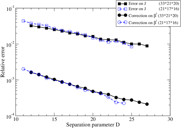
FIG. 10.: Relative difference between the regularized shift and the exact solution of (4) (circles) and relative difference between $J$ calculated by means of (67) and (68) (squares). The filled symbols and the solid line denote the high resolution and the empty symbols and the dashed line the low resolution.

We have plotted the relative difference $\delta J/J$ between the two integrals (67) and (68) in Fig. 10 as a function on the separation between the two holes. Also shown on the same figure is the relative norm of the correction function $|\vec{\beta}_{\rm cor}|/|\vec{\beta}|$. The correlation between the two curves shows that the error on the momentum constraint arises from the introduction of the correction function on the shift. It is also clear from Fig. 10 that increasing the number of coefficients in the spectral method does not make the correction function tend to zero. This means that the error in the momentum constraint come rather from the method (necessity to regularize the shift vector) than from some lack of numerical precision.

As discussed in Paper I, we had to regularize the shift vector because Eq. (41) is not enforced in our scheme. It has been argued recently by Cook [22] that if one reformulates the problem by assuming that the helical vector ${\ell}$ is not an exact Killing vector, but only an approximate one — as it is in reality — then the only freely specifiable part of the extrinsic curvature, as initial data, is (6), not (41). This means that the relation (41) between the extrinsic curvature and the shift is not as robust as the relation (6).

However, we see from Fig. 10 that at the innermost stable circular orbit, which is located at $D=17$ (cf. Sec. IV C), the error are very small:

$$\delta J/J = 2\ 10^{-2}$$ (69)

$$|\vec{\beta}_{\rm cor}| = 8\ 10^{-4}|\vec{\beta}|\ .$$ (70)

The $\delta J/J$ error estimator maximizes the error on the momentum constraint because it integrates it in all space. Thus we conclude that momentum constraint is satisfied in our numerical results with a precision of the order $1\%$.

2 Check of the Smarr formula

A good check of the global error in the numerical solution is the generalized Smarr formula derived in Paper I :

$$M-2\Omega J=-\frac{1}{4\pi}\oint_{S_{1}}\Psi^{2}\bar{D}_{i}Nd\bar{S}^{i}-\frac{1}{4\pi}\oint_{S_{2}}\Psi^{2}\bar{D}_{i}Nd\bar{S}^{i}.$$ (71)

For any computation, one gets $M$, $\Omega$ and can compute the r.h.s. of Eq. (71) and use that equation to derive the value of $J$ that fulfills the Smarr formula. That value is then compared to the ones calculated using Eqs. (67) and (68). The comparison is plotted in Fig. 11 for the two different resolutions. It turns out that the angular momentum calculated at infinity is better in fulfilling the Smarr formula than the one calculated on the throats by an order of magnitude and that the precision is better than $5\times 10^{-3}$. So, for all following purposes, we will use the value of $J$ given by Eq. (67).

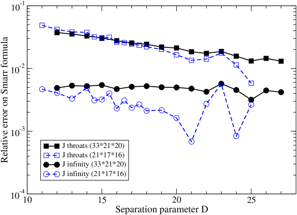
FIG. 11.: Relative error on the generalized Smarr formula (71). The circles denote the error obtained using $J$ calculated at infinity [Eq. (67)] and the squares that obtained when evaluating $J$ on the throats [Eq. (68)]. The filled symbols and the solid line denote the high resolution and the empty symbols and the dashed line the low resolution.

3 Check of Kepler law at large separation

The next thing one wishes to test is the value of $\Omega$, obtained from the virial criterium (14). In Newtonian gravity, two points particles on circular orbits obey the following relation, which is equivalent to Kepler’s third law:

$$\frac{4J\Omega^{1/3}}{M^{5/3}}=1,$$ (72)

where $M$ is the total mass, $J$ the total angular momentum and $\Omega$ the orbital velocity. For large separations of the two throats we expect to recover this relation. Therefore, for every value of $D$, we evaluate

$$I:=\frac{4J\Omega^{1/3}}{M^{5/3}}$$ (73)

and check if $I$ tends to $1$ when $D\rightarrow\infty$.

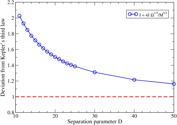
FIG. 12.: Value of $I=4J\left(\Omega/M^{5}\right)^{1/3}$ (low resolution runs) with respect to the separation parameter $D$. The horizontal dashed line corresponds to the value predicted by Kepler’s third law.

The value of $I$ is plotted in Fig. 12 with respect to the distance parameter $D$. As expected, for large values of $D$, it tends to $1$, implying that for large separations the system behaves like two point particles in Keplerian motion.

C Evolutionary sequence

Let us first present some figures about the metric fields. Figure 13 shows the total lapse function $N$, conformal factor $\Psi$ and the shift vector $\vec{\beta}$ and Fig. 14 the components $\hat{A}^{xx}$, $\hat{A}^{xy}$ and $\hat{A}^{yy}$ of the extrinsic curvature tensor. All those plots are cross-section in the orbital plane $z=0$ and the coordinate system is a Cartesian one centered at the middle of the centers of the throats. The computation has been done using the high resolution. The separation parameter is $D=17$. As it will be seen later, this separation corresponds to the turning point in the energy and angular momentum curves.

FIG. 13.: Isocontour of the lapse function $N$ and of the conformal factor $\Psi$ and plot of the shift vector $\vec{\beta}$, for $D=17$, in the orbital plane $z=0$. The computation has been done using the high resolution. The thick solid lines denote the surfaces of the throats. The kilometer scale of the axis corresponds to an ADM mass of $31.8M_{\odot}$.

FIG. 14.: Isocontour of the extrinsic curvature tensor for $D=17$ in the orbital plane $z=0$. The solid (dashed) lines denote positive (negative) values. The thick solid lines denote the surfaces of the throats. The computation has been done using the high resolution. The kilometer scale of the axis corresponds to an ADM mass of $31.8M_{\odot}$.

In the previous section, the only parameter we considered was the dimensionless separation parameter $D$. But there also exists a scaling factor. Suppose that all the distances in the computation are multiplied by some factor $\alpha$. Another solution with the same value of $D$ will be obtained, the global quantities being rescaled as

$$M_{\alpha} = \alpha M_{1}$$ (74)

$$J_{\alpha} = \alpha^{2}J_{1}$$ (75)

$$\Omega_{\alpha} = \frac{\Omega_{1}}{\alpha},$$ (76)

where $M_{1}$, $J_{1}$ and $\Omega_{1}$ are the values before rescaling and $M_{\alpha}$, $J_{\alpha}$ and $\Omega_{\alpha}$ the values after the rescaling.

Consider a physical configuration corresponding to a value $D\left(n\right)$ of the separation parameter, with global quantities $M\left(n\right)$, $J\left(n\right)$ and $\Omega\left(n\right)$. This system will evolve due to the emission of gravitational radiation. A subsequent configuration $n+1$ will have $D\left(n+1\right)<D\left(n\right)$. But what scaling factor $\alpha$ should be applied to the configuration calculated for $D\left(n+1\right)$ to ensure that it represents the same physical system as before ? In other word, a physical sequence is a one parameter (the separation) family of configurations and we have to impose another condition to determine the scaling factor associated with each value of $D$. In the case of binary neutron stars the condition is obtained by imposing that the number of baryons is conserved (see e.g. Ref. [14]). This cannot be extended to the black holes case since no matter is present. We chose instead to define a sequence by requiring that the loss of energy (ADM mass) $dM$ and angular momentum $dJ$ due to gravitational wave emission are related by

$$\left.\frac{dM}{dJ}\right|_{\rm sequence}=\Omega.$$ (77)

This relation is exact at least when one considers only the quadrupole formula (see e.g. page 478 of Ref. [26]). It turns out that it is also well verified for sequences of binary neutron stars [27, 28]. So Eq. (77) should hold rather well for corotating black holes.

The scaling factor $\alpha$ associated with the separation parameter $D\left(n+1\right)$ can be computed from the global values at separation $D\left(n\right)$ and the unscaled values at separation $D\left(n+1\right)$ as the solution the third degree equation

$$\frac{M\left(n\right)-\alpha M_{1}\left(n+1\right)}{J\left(n\right)-\alpha^{2}J_{1}\left(n+1\right)}=\frac{1}{2}\left(\Omega\left(n\right)+\frac{\Omega_{1}\left(n+1\right)}{\alpha}\right),$$ (78)

which is a first-order translation of Eq. (77). To present the results, we define the following dimensionless quantities

$$\bar{M}:=\frac{M}{M_{0}}$$ (79)

$$\bar{J}:=\frac{J}{M_{0}^{2}}$$ (80)

$$\bar{\Omega}:=M_{0}\Omega$$ (81)

$$\bar{l}:=\frac{l}{M_{0}},$$ (82)

where $l$ is the proper separation of the holes, defined as the geometrical distance between the throats along the axis joining their centers. $M_{0}$ is some arbitrary mass used for normalization purpose. It is often convenient to choose $M_{0}$ to be the total mass of the system when the two holes are infinitely separated, i.e. the ADM mass when $D\rightarrow\infty$. Unlike other methods, this value is not an input parameter of our calculation. It can only be obtained by constructing a sequence until very large values of $D$, which would impose to calculate a great number of configurations. However, as will been seen further, the system will exhibit turning point in the total energy and angular momentum, thereafter assumed to be the signature of an innermost stable circular orbit (thereafter ISCO). We chose $M_{0}$ to be the total ADM mass of the system at that point :

$$M_{0}:=\left.M_{\rm ADM}\right|_{\rm ISCO},$$ (83)

so that $\bar{M}$ is $1$ at the location of the ISCO.

The values of the dimensionless quantities $\bar{\Omega}$, $\bar{J}$, $\bar{M}$ and $\bar{l}$ along the sequence are given by Table I, for the high resolution.

TABLE I.: Values of dimensionless quantities along a sequence of corotating black holes obtained using the high resolution. The bold line denotes the values at the location of the ISCO.

$D$	$\bar{\Omega}$	$\bar{J}$	$\bar{M}$	$\bar{l}$
$40$	$0.0296159$	$0.995862$	$1.00597$	$13.3502$
$39$	$0.0307026$	$0.987981$	$1.00573$	$13.0699$
$38$	$0.0318074$	$0.978701$	$1.00544$	$12.7892$
$37$	$0.0330632$	$0.971834$	$1.00522$	$12.5075$
$36$	$0.0344638$	$0.966535$	$1.00504$	$12.2247$
$35$	$0.0358923$	$0.959407$	$1.00479$	$11.9414$
$34$	$0.0374279$	$0.952494$	$1.00453$	$11.6572$
$33$	$0.0390612$	$0.945264$	$1.00426$	$11.3721$
$32$	$0.0408436$	$0.938754$	$1.004$	$11.086$
$31$	$0.0427491$	$0.931913$	$1.00371$	$10.7988$
$30$	$0.0448273$	$0.925596$	$1.00343$	$10.5104$
$29$	$0.0470335$	$0.918635$	$1.00311$	$10.2211$
$28$	$0.0494625$	$0.911941$	$1.00279$	$9.93012$
$27$	$0.0521747$	$0.907183$	$1.00255$	$9.6379$
$26$	$0.0550996$	$0.901696$	$1.00225$	$9.34411$
$25$	$0.0582842$	$0.896173$	$1.00194$	$9.04881$
$24$	$0.0617501$	$0.89047$	$1.0016$	$8.75188$
$23$	$0.0656222$	$0.885511$	$1.00128$	$8.45286$
$22$	$0.0699629$	$0.88151$	$1.00101$	$8.15164$
$21$	$0.0747426$	$0.877312$	$1.00071$	$7.84823$
$20$	$0.0801137$	$0.874079$	$1.00046$	$7.54243$
$19$	$0.086184$	$0.871511$	$1.00024$	$7.23364$
$18$	$0.0930453$	$0.869573$	$1.00007$	$6.9218$
${\bf 17}$	${\bf 0.100897}$	${\bf 0.86885}$	${\bf 1}$	${\bf 6.60644}$
$16$	$0.109958$	$0.869769$	$1.0001$	$6.28724$
$15$	$0.120329$	$0.870729$	$1.00021$	$5.96358$
$14$	$0.132657$	$0.874838$	$1.00073$	$5.63471$
$13$	$0.14712$	$0.880134$	$1.00147$	$5.30006$
$12$	$0.164512$	$0.888448$	$1.00276$	$4.95863$

FIG. 15.: $\bar{M}$ with respect to $\bar{J}$ along a sequence. The filled symbols and solid line denote the high resolution and the empty symbols and the dashed line the low one.

FIG. 16.: $\bar{M}$ with respect to $\bar{\Omega}$ along a sequence. The filled symbols and solid line denote the high resolution and the empty symbols and the dashed line the low one.

FIG. 17.: $\bar{J}$ with respect to $\bar{\Omega}$ along a sequence. The filled symbols and solid line denote the high resolution and the empty symbols and the dashed line the low one.

6.60644

FIG. 18.: $\bar{l}$ with respect to $\bar{\Omega}$ along a sequence. The filled symbols and solid line denote the high resolution and the empty symbols and the dashed line the low one.

Figures 15, 16, 17 and 18 show the values of the dimensionless quantities along a sequence. The calculation has been performed with the high and low resolutions and for values of the parameter $D$ ranging from $40$ to $11$. As previously mentioned, the sequence exhibits a minimum of $\bar{J}$ and $\bar{M}$ as the throats become closer, thereafter interpreted as the signature of an innermost stable circular orbit (ISCO) [29]. But at this point, we have to be cautious. Indeed, the relative variation of $\bar{M}$ and $\bar{J}$ along a sequence is rather small, and comparable to the precision estimated by means of the Smarr formula (see Sec. IV B). The exact location of the ISCO being very dependent on those small effects, we do not claim to have very precisely determined it. The following results should be confirmed with more precise calculations.

Another important quantity is the area of the black hole horizons which relates to the irreducible mass [30] (see also Box 33.4 of [31]). As discussed in Sec. II.B.6 of Paper I, in our case the apparent horizons coincide with the two throats. We therefore define the dimensionless irreducible mass by

$$\bar{M}_{\rm ir}:=\frac{1}{M_{0}}\left(\sqrt{\frac{A_{1}}{16\pi}}+\sqrt{\frac{A_{2}}{16\pi}}\right)\ ,$$ (84)

where $A_{a}$ ($a=1,2$) denotes the area of the throat $a$, calculated according to the formula

$$A_{a}=\oint_{S_{a}}\Psi^{4}d\bar{S}.$$ (85)

FIG. 19.: Relative change of $\bar{M}_{\rm ir}$ along the sequence, with respect to the orbital velocity $\bar{\Omega}$. The filled symbols and the solid line denote the high resolution and the empty symbols and the dashed line the low resolution.

Figure 19 shows the relative change of $\bar{M}_{\rm ir}$ along the sequence. It exhibits a slight increase, but its variation is very small. It appears that, along the overall sequence, the variation is smaller than $10^{-3}$. The precision of our code being of that order, this result is compatible with the fact that $\bar{M}_{\rm ir}$ is constant. In other word it shows that imposing the condition (77) is equivalent to imposing that the irreducible mass is constant along a sequence. This constitutes in fact a very good test of our procedure. Indeed Friedman, Uryu & Shibata [32] have recently established the first law of binary black hole thermodynamics:

$$dM=\Omega dJ+\kappa_{1}dA_{1}+\kappa_{2}dA_{2}\ ,$$ (86)

where $\kappa_{1}$ and $\kappa_{2}$ are two constants, representing the black holes surface gravity. For identical black holes ($\kappa_{1}=\kappa_{2}$ and $dA_{1}=dA_{2}$), the above relation implies

$$dM=\Omega dJ\quad\Longleftrightarrow\quad dA_{a}=0\quad(a=1,2)\ .$$ (87)

Hence the area of each black hole must be conserved during the evolution. In future works, this last criterium could be used to define a sequence, instead of the relation (77).

We choose an average value of the irreducible mass $\bar{M}_{\rm ir}=1.0173$ and we define then the binding energy of the system at the ISCO by

$$\left.\bar{E}_{\rm b}\right|_{\rm ISCO}=1-\bar{M}_{\rm ir},$$ (88)

the dimensionless total energy being equal to $1$ at the location of the turning point.

The values of the dimensionless quantities $\bar{\Omega}$, $\bar{J}$, $\bar{E}_{\rm b}$ and $\bar{l}$ at the ISCO are given in Table II and compared with the results from other approaches (see [29] for a review). 3-PN EOB stands for the third order post-Newtonian Effective One Body method for non-spinning black holes [33], with two values of the 3-PN parameter $\omega_{s}$: $\omega_{s}=0$ and $\omega_{s}=-9.34$. 3-PN j-method stands for third order post-Newtonian j-method of [33]. Puncture denotes the results from the puncture method in the case of non-spinning black holes [34] and Conformal imag. the conformal imaging approach with various values of the individual spins for rotating black holes [11]. By definition $\bar{M}=1$ at the location of the ISCO for all the methods. The results from the different methods are also plotted in Fig. 20.

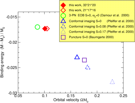
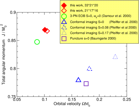
FIG. 20.: Values of $\bar{E}_{\rm b}$ and $\bar{J}$ with respect to $\bar{\Omega}$ at the ISCO for different methods, including ours with high and low resolution. The references to previous studies are as follows: Damour et al. 2000: [33], Pfeiffer et al. 2000: [11] and Baumgarte 2000: [34]. $S$ denotes the (fixed) spin of the black holes used in various methods.

TABLE II.: Values of dimensionless quantities at the location of the ISCO. Comparison with other works.

Method	$\bar{\Omega}$	$\bar{J}$	$\bar{E}_{\rm b}$	$\bar{l}$
3-PN EOB $\omega_{s}=0$ $S=0$ [33]	$0.0868$	$0.847$	$-0.0170$	not given
3-PN EOB $\omega_{s}=-9.34$ $S=0$ [33]	$0.0722$	$0.877$	$-0.0152$	not given
3-PN j-method $\omega_{s}=-9.34$ $S=0$ [33]	$0.0731$	$0.877$	$-0.0153$	not given
Puncture $S=0$ [34]	$0.176$	$0.773$	$-0.0235$	$4.913$
Conformal imag. $S=0$ [11]	$0.162$	$0.779$	$-0.0230$	$5.054$
Conformal imag. $S=0.08$ [11]	$0.182$	$0.799$	$-0.0250$	$4.705$
Conformal imag. $S=0.17$ [11]	$0.229$	$0.820$	$-0.0279$	$4.040$
This work (high res.)	$0.101$	$0.869$	$-0.0173$	$6.606$
This work (low res.)	$0.105$	$0.867$	$-0.0173$	$6.450$

Figure 20 shows explicitly that the present results are in much better agreement with post-Newtonian calculations than with other numerical works. Note that the post-Newtonian point plotted on Fig. 20 corresponds to the value $0$ of the (previously ambiguous) 3-PN “static” parameter $\omega_{s}$. This is indeed the value recently determined by Damour et al. [35].

But let us point out that it is rather difficult to compare precisely our results with the other works. The main problem comes from the fact that all those methods use individual spins of the black holes as input parameters. In the present paper we impose corotation, that is that the throats are spinning at the orbital velocity. The only value that can be computed is the total angular momentum $J$ and, in general relativity, it cannot be split into orbital and spins parts in a invariant way. However, from the results of Pfeiffer et al. [11] one can see that increasing the spins of the black holes make the values $\bar{\Omega}$, $\bar{J}$ and $-\bar{E}_{\rm b}$ at the ISCO greater. Taking rotation into account in the post-Newtonian methods [36] will probably make the orbital velocity and the binding energy at the ISCO match even better with our values. Work is under progress to compare with corotating post-Newtonian results [37].

So, it appears that our results match pretty well with post-Newtonian methods. This is the most striking conclusion from our study. The difference between numerical and post-Newtonian results have often been imputed mostly to the conformal flatness approximation (see [29]). The fact that our result, using conformal flatness, is in much better agreement with PN calculations than other numerical works, makes us believe that the main worry of both conformal imaging and puncture methods lies elsewhere, possibly in the determination of $\Omega$. Indeed, it is very unlikely that the orbits and so orbital velocity can be properly computed by solving only for the four constraint equations. Time should be involved at some level and one should take other Einstein equations into account, as we have done here.

V Conclusions

The present work should be seen as a first step in trying to give some new insight to the binary black holes problem. The basic idea is to extend the numerical treatment beyond the resolution of the four constraint equations within a 3-dimensional spacelike surface. This is achieved by reintroducing time in the problem to deal with a 4-dimensional spacetime. The orbits are well defined by imposing the existence of a helical Killing vector and the orbital velocity is found as the only value that equals the ADM and the Komar-like masses, a requirement which is equivalent to the virial theorem. According to us those are the two most important features of our method. The approximation of conformal flatness for the 3-metric has only been used for simplicity. Sooner or later this problem will have to be solved using a general spatial metric and outgoing waves boundary conditions at large distances. The use of the inversion isometry to derive boundary conditions on the throats is also a weak assumption. In the future, it would be interesting to change the boundary conditions on the fields in order to investigate their influence on the results (see e.g. [22] for an alternative choice). Besides, changing the boundary conditions on the shift vector should enable us to describe other states of rotation of the black holes, as has been recently proposed by Cook [22].

The numerical schemes are basically the same as those which have been previously successfully applied to binary neutron stars configurations [14]. They have been extended to solve elliptic equations with non-trivial boundary conditions imposed on two throats and exact boundary conditions at infinity. Those techniques passed numerous tests and recover the Schwarzschild and Kerr solutions as well as the Misner-Lindquist one for two static black holes [5, 6]. A technical problem lies in the great number of coefficients needed to accurately describe the part of the sources located around the companion hole. This effect causes some lack of precision. But we can estimate the error it generates by varying the number of coefficients, and comparing the results. This is what we have done here, using $21\times 17\times 16$ coefficients in each of the 12 domains for the low resolution computations and $33\times 21\times 20$ coefficients for the high resolution ones. The accuracy, estimated from the generalized Smarr formula, is below $1\%$.

Another issue is the slight violation of the momentum constraint which arises from the necessity to regularize the shift vector. We have found that the modification of the shift vector with respect to the vector which satisfies the momentum constraint (4) is below $10^{-3}$, and that the error it induces in the momentum constraint equation is of the order $1\%$. In view of the other approximations performed in this work, especially the conformal flatness of the 3-metric, we find this to be very satisfactory.

In this article, we have defined a sequence of binary black holes by requiring that the ADM mass decrease is related to the angular momentum decrease via $dM=\Omega\,dJ$. This relation is true for the loss due to gravitational radiation, at least when one considers only the quadrupole formula. We have then found that the area of the apparent horizons (irreducible mass) is constant along the sequence, in agreement with the first law of binary black holes thermodynamics recently derived by Friedman et al. [32].

The location of the ISCO has been obtained and compared with the results from other methods [33, 34, 11]. It turns out that our results match the 3-PN methods much better than previous numerical works. The differences between numerical studies and 3-PN approximations have often been explained by the use of the conformal flatness approximation in the numerical calculations [33]. It seems to us that this is not the main explanation, for we are using this approximation. It certainly arises instead from the way $\Omega$ is determined.

Another natural extension of this work is to use the obtained configurations as initial data for binary black holes evolution codes (see [38] for a review and Refs. [39, 40, 41] for recent results). Initial data files containing the result of the present work are publically available on the CVS repository of the European Union Network on Sources of Gravitational Radiation [42]. Extraction of the wave-forms from a sequence would also be an interesting application [43, 44].

- [1] E. Gourgoulhon, P. Grandclément and S. Bonazzola, submitted to Phys. Rev. D, preprint gr-qc/0106015 [Paper I].
- [2] S. Detweiler, in Frontiers in Numerical Relativity, edited by C.R. Evans, L.S. Finn, and D.W. Hobill (Cambridge University Press, Cambridge, 1989), p. 43.
- [3] J.W. York, in Sources of Gravitational Radiation, edited by L.L. Smarr (Cambridge University Press, Cambridge, 1979), p. 83.
- [4] G.J. Mathews, P. Maronetti and J.R. Wilson, Phys. Rev. D 58, 043003 (1998).
- [5] C.W. Misner, Ann. Phys. (N.Y.) 24, 102 (1963).
- [6] R.W Lindquist, J. Math. Phys. 4, 938 (1963).
- [7] A.D. Kulkarni, L.C. Shepley, and J.W. York, Phys. Lett. 96A, 228 (1983).
- [8] G.B. Cook, Phys. Rev. D 44, 2983 (1991).
- [9] G.B. Cook, M.W. Choptuik, M.R. Dubal, S. Klasky, R.A. Matzner, and S.R. Oliveira, Phys. Rev. D 47, 1471 (1993).
- [10] G.B. Cook, Phys. Rev. D 50, 5025 (1994).
- [11] H.P. Pfeiffer, S.A. Teukolsky, and G.B. Cook, Phys. Rev. D 62, 104018 (2000).
- [12] P. Diener, N. Jansen, A. Khokhlov, and I. Novikov, Class. Quantum Grav. 17, 435 (2000).
- [13] E. Gourgoulhon and S. Bonazzola, Class. Quantum Grav. 11, 443 (1994).
- [14] E. Gourgoulhon, P. Grandclément, K. Taniguchi, J.-A. Marck, and S. Bonazzola, Phys. Rev. D 63, 064029 (2001).
- [15] C. Canuto, M.Y. Hussaini, A. Quarteroni and T.A. Zang Spectral Methods in Fluid Dynamics (Spinger-Verlag,Berlin,1988)
- [16] S. Bonazzola, E. Gourgoulhon and J.-A. Marck, Phys. Rev. D 58, 104020 (1998).
- [17] S. Bonazzola, E. Gourgoulhon and J.-A. Marck, J. Comput. Appl. Math. 109, 433 (1999).
- [18] P. Grandclément, S. Bonazzola, E. Gourgoulhon and J.-A. Marck, J. Comp. Phys. 170, 231 (2001).
- [19] N. Jansen, P. Diener, A. Khokhlov, and I. Novikov, preprint: gr-qc/0103029.
- [20] K. Oohara and T. Nakamura, in Relativistic Gravitation and Gravitational Radiation, edited by J.-A. Marck and J.-P. Lasota (Cambridge University Press, Cambridge, 1997), p. 309.
- [21] K. Oohara, T. Nakamura and M. Shibata, Prog. Theor. Phys. Suppl. 128, 183 (1987).
- [22] G.B. Cook, preprint gr-qc/0108076.
- [23] A. Garat and R.H. Price, Phys. Rev. D 61, 124011 (2000).
- [24] D. Giulini, in Black Holes: Theory and Observation, edited by F.W. Hehl, C. Kiefer and R.J.K. Metzler (Spinger-Verlag, Berlin, 1998), p. 224.
- [25] Z. Andrade and R. Price, Phys. Rev. D 56, 6336 (1997).
- [26] S.L. Shapiro and S.A. Teukolsky, Black Holes, White Dwarfs and Neutron Stars, (J. Wiley and Sons, New-York,1983).
- [27] T.W. Baumgarte, G.B. Cook, M.A. Scheel, S.L. Shapiro, and S.A. Teukolsky, Phys. Rev. D 57, 7299 (1998).
- [28] K. Uryu, M. Shibata, and Y. Eriguchi, Phys. Rev. D 62, 104015 (2000).
- [29] T.W. Baumgarte, in Astrophysical Sources of Gravitational Radiation, edited by J.M. Centrella, AIP press, in press, preprint gr-qc/0101045.
- [30] C. Christodoulou, Phys. Rev. Lett. 25, 1596 (1970).
- [31] C.W. Misner, K.S. Thorne, and J.A. Wheeler, Gravitation (Freeman, New York, 1973).
- [32] J.L. Friedman, K. Uryu, and M. Shibata, preprint gr-qc/0108070.
- [33] T. Damour, P. Jaranowski and G. Schäfer Phys. Rev. D 62, 084011 (2000).
- [34] T.W. Baumgarte Phys. Rev. D 62, 024018 (2000).
- [35] T. Damour, P. Jaranowski and G. Schäfer, Phys. Lett. B 513, 147 (2001).
- [36] T. Damour, Phys. Rev. D, in press (preprint: gr-qc/0103018).
- [37] T. Damour, E. Gourgoulhon, and P. Grandclément, in preparation.
- [38] E. Seidel, in Black Holes and Gravitational Waves – New Eyes in the 21st Century, Proc. of the 9th Yukawa International Seminar, Kyoto 1999, edited by T. Nakamura and H. Kodama, Prog. Theor. Phys. Suppl. 136, 87 (1999).
- [39] S. Brandt, R. Correll, R. Gómez, M. Huq, P. Laguna, L. Lehner, P. Marronetti, R.A. Matzner, D. Neilsen, J. Pullin, E. Schnetter, D. Shoemaker, and J. Winicour, Phys. Rev. Lett. 85, 5496 (2000).
- [40] M. Alcubierre, W. Benger, B. Brügmann, G. Lanfermann, L. Nerger, E. Seidel, and R. Takahashi, preprint gr-qc/0012079.
- [41] J. Baker, B. Brügmann, M. Campanelli, C. O. Lousto, and R. Takahashi, Phys. Rev. Lett. 87, 121103 (2001).
- [42] http://www.eu-network.org/Projects/InitialData.html
- [43] M.D. Duez, T.W. Baumgarte and S.L. Shapiro Phys. Rev. D 63, 084030 (2001).
- [44] M. Shibata and K. Uryu, Phys. Rev. D, in press (preprint: gr-qc/0109026).