General relativistic viscous hydrodynamics of differentially rotating neutron stars
Abstract
Employing a simplified version of the Israel-Stewart formalism for general-relativistic shear-viscous hydrodynamics, we perform axisymmetric general-relativistic simulations for a rotating neutron star surrounded by a massive torus, which can be formed from differentially rotating stars. We show that with our choice of a shear-viscous hydrodynamics formalism, the simulations can be stably performed for a long time scale. We also demonstrate that with a possibly high shear-viscous coefficient, not only viscous angular momentum transport works but also an outflow could be driven from a hot envelope around the neutron star for a time scale ms with the ejecta mass which is comparable to the typical mass for dynamical ejecta of binary neutron star mergers. This suggests that massive neutron stars surrounded by a massive torus, which are typical outcomes formed after the merger of binary neutron stars, could be the dominant source for providing neutron-rich ejecta, if the effective shear viscosity is sufficiently high, i.e., if the viscous parameter is . The present numerical result indicates the importance of a future high-resolution magnetohydrodynamics simulation that is the unique approach to clarify the viscous effect in the merger remnants of binary neutron stars by the first-principle manner.
pacs:
04.25.D-, 04.30.-w, 04.40.DgI Introduction
The recent discoveries of two-solar mass neutron stars twosolar imply that the equation of state of neutron stars has to be stiff enough to support the self-gravity of the neutron stars with mass . Numerical-relativity simulations with stiff equations of state that provides the maximum neutron-star mass larger than have shown that massive neutron stars surrounded by a massive torus are likely to be the canonical remnants formed after the merger of binary neutron stars of typical total mass 2.6– (see, e.g., Refs. STU2005 ; Hotokezaka2013 ). Because a shear layer is inevitably formed on the contact surface of two neutron stars at the onset of the merger, the Kelvin-Helmholtz instability PR ; kiuchi is activated and the resulting vortex motion is likely to quickly amplify the magnetic-field strength toward G. In addition, because the remnant massive neutron stars and a torus surrounding them are in general differentially rotating and magnetized, they shall be subject to magnetorotational instability (MRI) BH98 . As shown by a number of high-resolution magnetohydrodynamics (MHD) simulations for accretion disks (see, e.g., Refs. alphamodel ; suzuki ; local ), MHD turbulence is likely to be induced for differentially rotating systems and its effect will determine the subsequent evolution of the system (but see also Ref. GBJJ for a possibly significant role of neutrinos for relatively low-magnetic field cases). As a result, (i) angular momentum is likely to be transported outward and thermal energy will be generated by dissipating rotational kinetic energy in the massive neutron star and surrounding torus and (ii) a massive hot torus is likely to be further developed around the massive neutron stars.
For exploring MHD processes and resulting turbulent state for the remnants of binary neutron star mergers, non-axisymmetric (extremely) high-resolution simulation is necessary if we rely entirely on a MHD simulation (see, e.g., Ref. kiuchi for an effort on this). The reasons for this are that the wavelength for the fastest growing modes of the Kelvin-Helmholtz instability and MRI is much shorter than the stellar size for the typical magnetic-field strength (– G), and in addition, the MHD turbulence is preserved only in a non-axisymmetric environment: Here, note that in axisymmetric systems, the turbulence is not preserved for a long time scale according to the anti-dynamo theorem anti . This implies that we would need a huge computational cost for studying realistic evolution of the merger remnants of binary neutron stars (see, e.g., Ref. kiuchi ), and it is practically not an easy task to obtain a comprehensive picture for the evolution of this system by systematically performing a large number of MHD simulations changing neutron-star models and the magnetic-field profiles. To date, this problem has not been solved because the well-resolved MHD simulation has not been done yet.
One phenomenological approach for exploring the evolution of differentially rotating systems such as the merger remnants is to employ viscous hydrodynamics in general relativity DLSS04 . The global-scale viscosity is likely to be effectively generated through the development of the turbulent state induced by the local MHD processes, and thus, relying on the viscous hydrodynamics implies that we employ a phenomenological approach, averaging (coarse graining) the local MHD and turbulence processes. A demerit in this approach is that we have to artificially input the viscous coefficient, which would be naturally determined in the MHD simulations. Thus, we cannot obtain the real answer by one simulation in this approach. We can at best obtain answers for given values of the viscous coefficient, which has to be varied for a wide range to obtain a possible variety of the answers. However, we also have several merits in this approach. First, we may perform an axisymmetric simulation to follow the long-term transport processes. We also would not need extremely high-resolution simulations in this approach, because we do not have to consider short-wavelength MHD instabilities. Thus, we can reduce the computational costs significantly, and hence, with relatively small computational costs, we are able to systematically explore the phenomenological evolution of differentially rotating systems including differentially rotating neutron stars, a torus surrounding them, and black hole-torus systems.
One caveat for employing viscous hydrodynamics in relativity is that it could violate the causality if we choose an inappropriate set of the basic equations. Indeed, in relativistic Navier-Stokes-type equations DLSS04 ; LL59 in which basic equations are parabolic-type, the causality is violated. On the other hand, if we employ Israel-Stewart-type formulations Israel1976 , the resulting equation is not parabolic-type but telegraph-type, and hence, the causality is preserved hiscock83 . In this paper, we employ a simplified version of the Israel-Stewart formulation to incorporate shear-viscosity effects neglecting the bulk viscosity and other transport processes. It is shown that in this case, the hydrodynamics equations are significantly simplified and they can be numerically solved in a method quite similar to those for pure hydrodynamics, while the major effects of the shear viscosity can be qualitatively captured.
The primary purpose of this paper is to show that our choice of viscous hydrodynamics formalism works well for long-term simulations of differentially rotating systems. We perform simulations for rotating neutron stars surrounded by a torus for a long time scale, focusing in particular on the long-term mass ejection process from the torus. In this paper, we do not take into account detailed microphysics effects such as neutrino transport and we focus only on the purely viscous hydrodynamics. We plan to present the results of more detailed studies incorporating microphysics effects in the future publication.
This paper is organized as follows: In Sec. II, we describe our formulation for simplified shear-viscous hydrodynamics. In Sec. III, we apply our formulation to an axisymmetric general-relativistic simulation for a differentially rotating neutron star, and show that with a plausible shear viscosity, an outflow may be driven from a massive neutron star and a torus surrounding it that are the typical outcomes of binary neutron star mergers. Section IV is devoted to a summary. Throughout this paper, we employ the units of where and are the speed of light and gravitational constant, respectively.
II Formulation
II.1 Viscous hydrodynamics for general case
We write the stress-energy tensor of viscous fluid as
| (1) |
where is the rest-mass density, is the specific enthalpy, is the four velocity, is the pressure, is the spacetime metric, is the viscous coefficient for the shear stress, and is the viscous tensor. In terms of the specific energy and pressure , is written as . is a symmetric tensor and satisfies . We suppose that is a function of , , and and will give the relation below.
Taking into account the prescription of Ref. Israel1976 , we assume that obeys the following evolution equation:
| (2) |
where denotes the Lie derivative with respect to , and we set as
| (3) |
with and the covariant derivative associated with . By introducing Eq. (2), the viscous hydrodynamics equation becomes a telegraph-type equation Israel1976 ; hiscock83 . Here, is a non-zero constant of (time)-1 dimension and it has to be chosen in an appropriate manner so as for to approach in a short time scale because it is reasonable to suppose that should approach in a microphysical time scale. Thus, we typically choose it so that is shorter than the dynamical time scale of given systems (but it should be much longer than the time-step interval of numerical simulations, , in the practical computation).
Equation (2) can be rewritten as
| (4) |
where . We employ this equation for as one of the basic equations of viscous hydrodynamics, and hence, the stress-energy tensor is rewritten as follows:
Using the timelike unit vector field normal to spatial hypersurfaces, , and the induced metric on the spatial hypersurfaces , we define
| (6) | |||||
| (7) | |||||
| (8) |
Here, the time and spatial components of are written as where and are the lapse function and the shift vector, respectively. The explicit forms of and are
| (9) | |||||
| (10) |
where , , and with the bars denoting spatial components. Note that we used and . We also note that is equal to .
Then, a general-relativistic Navier-Stokes-type equation, derived from , is written in a form as
| (11) |
and the energy equation, derived from , is
| (12) |
where , is the covariant derivative associated with , and is the extrinsic curvature of spatial hypersurfaces. The transport terms are rewritten using
| (13) | |||||
| (14) | |||||
where and .
In addition to these equations, we have the continuity equation for the rest-mass density, , which is written as usual as
| (15) |
where .
In viscous hydrodynamics simulations, , , and are evolved (here is supposed to be obtained by solving Einstein’s evolution equations). This implies that it is straightforward to obtain the following quantities
| (16) | |||||
| (17) |
By contrast, and have to be calculated by using the normalization relation , which is written as
| (18) |
The procedure for a solution of and will be described later.
Spatial components of Eq. (4) are explicitly written in the form
| (19) |
Here, we focus only on the spatial components of this equation, because other components of are determined from . Multiplying and using the continuity equation (15) and , we obtain
| (20) |
Since is determined by solving the continuity equation, is obtained by solving this equation.
Next we describe how to determine and . These quantities are determined from Eqs. (16), (17), and (18). First, we write Eq. (17) as
| (21) |
where is a matrix and a function only of because is obtained by solving the evolution equation of . This implies that by inverting Eq. (21), is written as
| (22) |
and hence, for a given set of and , can be considered as a function of and . Substituting Eq. (22) into (18), we obtain a relation between and as
| (23) |
where can be considered as a function of .
II.2 Setting viscous parameter
In the so-called -viscous model, we have the relation (see, e.g., Ref. ST )
| (24) |
where denotes the local value of the angular velocity and is the so-called -viscous parameter, which is a dimensionless constant. In the -viscous model, we assume that the fluid is in a turbulent state and is written effectively as where is the size of the largest turbulent cells and is the velocity of the turbulent motion relative to the mean gas motion. Since and where is the maximum size of the object concerned (i.e., here the equatorial stellar radius) and is the sound velocity, may be written as where . For rapidly rotating systems, . With the definition of the sound velocity, , Eq. (24) is obtained. We suppose that should be of the order taking into account the latest results of high-resolution MHD simulations for accretion disks (e.g., Refs. alphamodel ; suzuki ; local ).
Thus, in the -viscous model, is written as
| (25) |
In this paper, we consider viscous hydrodynamics evolution of a differentially rotating neutron star. In practice, it is not easy to appropriately determine from the local angular velocity of neutron stars in a dynamical state, and hence, in this work, we simply set
| (26) |
where is the angular velocity at the equatorial stellar surface of the initial state of neutron stars (see, e.g., a filled circle in the left panel of Fig. 2). The relation, , is satisfied for rapidly rotating neutron stars and tori (or disks) located in the vicinity of the neutron stars. Thus, Eq. (26) agrees approximately with Eq. (25) for the outer region and the inner envelope of the neutron stars, to which we pay special attention in this paper. On the other hand, is underestimated for a region far from the rotation axis, to which we do not pay strong attention.
| (km) | (km) | (rad/s) | (rad/s) | ||||||
|---|---|---|---|---|---|---|---|---|---|
| 2.64 | 2.37 | 11.7 | 15.7 | 0.866 |
II.3 Axisymmetric equations
We solve viscous hydrodynamics equations in axisymmetric dynamical spacetime in the following manner. Einstein’s equation in axial symmetry is solved by a cartoon method cartoon ; cartoon2 , and hence, the basic field equations are solved in the plane of Cartesian coordinates. Thus, here, we describe viscous hydrodynamics equations in axial symmetry using Cartesian coordinates with . To do so, the basic equations are first written in cylindrical coordinates , and then, the coordinate transformation, and , should be carried out. The resulting equations are as follows: The continuity equation is written as
| (27) |
where and : is the determinant of the flat-space metric in the cylindrical coordinates. Each component of the viscous hydrodynamics equation is written in the forms
| (28) | |||
| (29) |
| (30) |
where , and
| (31) |
Here, the index denotes or , and , , and do , , or .
The energy equation is written in the form
| (32) |
where and . We note that the terms associated with in Eqs. (30) and (32) are responsible for the angular-momentum transport and viscous heating, respectively.
The method for a solution of these hydrodynamics equations is the same as in Refs. cartoon2 ; SS2012 : The transport terms are specifically evaluated using a Kurganov-Tadmor scheme KT with a piecewise parabolic reconstruction for the quantities of cell interfaces. We do not take into account the modification of the characteristic speed by the viscous effect for simplicity because the local transport time scale of fluid elements, , is much shorter than the viscous time scale, , in our choice of the alpha viscosity (here, denotes a characteristic length scale of the system). That is, the local characteristic speed of the fluid dynamics would be modified only slightly by the viscous effect.
The evolution equations for are written as
| (33) | |||
| (34) |
| (35) | |||
| (36) | |||
| (37) | |||
| (38) |
For the characteristic speed of these equations, we simply employ and for the - and -directions, respectively. From the regularity condition for the tensor quantity, we find the boundary conditions for at the symmetric axis, , as , , , and .
From Eqs. (27) and (30), it is immediately found that the baryon rest mass, , and angular momentum, , are conserved quantities, which are defined by
| (39) | |||
| (40) |
In numerical simulations, we monitor these quantities and check that they are preserved to be (approximately) constant. Note that these quantities are precisely conserved unless matter is ejected from the outer boundaries, because we solve the conservative forms for the equations of and . We also monitor the kinetic energy and internal energy defined, respectively, by
| (41) | |||||
| (42) |
These values clearly show how the viscous dissipation proceeds: and decrease by converting the kinetic energy to the internal energy.
We also calculate the mass and energy fluxes through a sphere far from the central object and evaluate the total mass and energy for the outflow component. The mass and energy fluxes are defined, respectively, by
| (43) | |||
| (44) |
Then, we calculate the outflowed mass and energy as functions of time by
| (45) | |||
| (46) |
Here, the internal energy of the outflow component is much smaller than the kinetic energy if we evaluate the outflow quantity in a far zone. Thus, we define the kinetic energy of the outflow by .

Before closing Sec. II, we should comment on the method of evaluating the derivative of , which appears in the equations for and does not appear in ideal fluid hydrodynamics. For the numerical results presented in this paper, we evaluate it by simple second-order centered finite differencing. However, is not always continuous and hence this treatment could introduce a non-convergent error. We monitor the violation of the Hamiltonian constraint, , in particular focusing on the following rest-mass-averaged quantity,
| (47) |
where and denotes individual components in like , , , and three-dimensional Ricci scalar. ERR shows the global violation of the Hamiltonian constraint. For ERR=0, the constraint is satisfied, while for ERR=1, the Hamiltonian constraint is by 100% violated. Figure 1 shows the evolution of ERR for the model with (see the next section for the details of our models). This figure illustrates that the convergence with respect to the grid resolution is far less than second order. However, the degree of the violation is reasonably small with ERR in our simulation time. This approximately indicates that the Hamiltonian constraint is satisfied within 1% error, and hence, we suppose that the results obtained in this paper would be reliable at least in our present simulation time.
For a long-term simulation, however, the violation is accumulated and eventually it could be so large that we are prohibited to derive a reliable numerical result or the computation crashes. For suppressing the numerical error, we will need to implement a better scheme of evaluating this slowly-convergent derivative term.
III Numerical simulation

III.1 Brief summary of simulation setting
Our method for a solution of Einstein’s equation is the same as that in Ref. SS2012 : We employ the original version of Baumgarte-Shapiro-Shibata-Nakamura formulation with a puncture-type gauge BSSN . The gravitational field equations are solved in the fourth-order finite differencing scheme. The axial symmetry is imposed using the cartoon method cartoon ; cartoon2 ; SS2012 , as already mentioned. A fourth-order Lagrange interpolation scheme is used for implementing the cartoon scheme.
A differentially rotating neutron star, which is used as an initial condition, is modeled employing a piecewise polytropic equation of state with two pieces:
| (50) |
where and are polytropic constants and and are polytropic indices, respectively. is a constant of the nuclear-density order: We here set it to be . In this work, we choose and , respectively.
For constructing initial models, we assume a very simple profile for the angular velocity given by where is the angular velocity along the rotation axis. As in Ref. PRL , we set , and then, the angular velocity is approximately given by
| (51) |
where denotes the equatorial coordinate stellar radius. For the simulation, we pick up a high-mass neutron star with the coordinate axial ratio 0.3 (i.e., the ratio of the polar coordinate radius to is 0.3). The important quantities for the initial condition is listed in Table I.
We note that the initial angular-velocity profile employed in this paper is qualitatively different from that of the merger remnants of binary neutron stars: For the realistic binary neutron star merger, the angular velocity near the rotation axis is rather slow, reflecting the fact that the velocity vectors of two neutron stars have the counter direction at the merger, and hence, shocks that dissipate their kinetic energy are formed STU2005 . Then, the merger remnant neutron star is weakly differentially rotating and surrounded by a thick torus. Starting from the differentially rotating neutron star employed in this paper, we soon have a (approximately) rigidly rotating neutron star surrounded by a massive torus, as we show below. Such outcome is similar to the merger remnant. One of the major purposes of this paper is to pay attention to long-term evolution of this type of the outcome.
During numerical evolution, we employ a modified version of the piecewise polytropic equation of state in the form
| (52) |
where denotes the specific internal energy associated with satisfying and the adiabatic constant is set to be . The second term is added to take into account a shock heating effect. We choose a relatively small value of in this work to mildly incorporate the shock heating effects.
Numerical simulations are performed in cylindrical coordinates , and a nonuniform grid is used for and . Specifically, we employ the following grid structure (the same profile is chosen for )
| (55) |
where is the grid spacing in an inner region with . with being the location of the -th grid point. At , . determines the nonuniform degree of the grid spacing and we set it to be . We change as (low resolution), (middle resolution), and (high resolution) to confirm that the dependence of the numerical results on the grid resolution is weak. We note that m in our model. The outer boundary is located at km for all the grid resolutions. Unless otherwise stated, we will show the results in the high-resolution runs in the following.
When using a nonuniform grid, numerical instability is often induced in a long-term simulation due to the gradual growth of high-frequency noises in the geometric variables, in particular in the extrinsic curvature. To suppress the growth of unstable modes associated with the numerical noises, we incorporate a six-order Kreiss-Oliger-type dissipation term as (see, e.g., Ref. bernd )
| (56) |
where is a constant of order unity and denotes the geometric quantities. in the present axisymmetric simulation is calculated by
| (57) |
Note that the coefficient in the second term of Eq. (56) is written in terms of (not ) because the accumulation of the high-frequency noise causes the problem only in the inner region. We find that with this prescription, the ERR in Eq. (47) can be kept to be for ms (see Fig. 1).
The viscous coefficient is written in the form of Eq. (26). We choose , 0.01, 0.02, and 0.03. is set to be . The viscous angular momentum transport time scale is approximately defined by Kato and estimated to be
| (58) | |||||
where we assumed Eq. (25) for . In the vicinity of the rotation axis (for a small value of and a high value of ), the time scale should be initially short. Thus, in ms, the angular momentum is expected to be transported outward in the differentially rotating neutron star initially prepared.
III.2 Numerical results


First, we summarize the typical viscous evolution process of our differentially rotating neutron star model, paying attention to the case of .
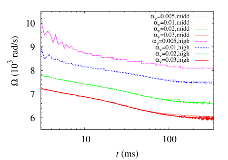
In the very early stage of its evolution, angular momentum in the central region of the neutron star is efficiently transported outward in where : the rotation period along the rotation axis. As a result, the initially differentially rotation state changes to an approximately rigidly rotation state for : see Fig. 2 for the evolution of the profile of the angular velocity along the -axis. In the present model, the angular velocity in the (approximately) rigidly rotating state is only slightly smaller than the Kepler velocity defined by which is rad/s initially. (For larger values of , the relaxed angular velocity is slightly smaller: see the right panel of Fig. 2.) After a nearly rigidly rotating state is achieved, the effect of the angular momentum transport inside the neutron star becomes weak and its angular velocity decreases only slowly as a result of the outward angular-momentum transport induced by the viscous effect that occurs in the outer region of the neutron star: see the right panel of Fig. 2. Since the angular velocity in the vicinity of the rotation axis is monotonically and steeply reduced in a few ms, we plot only the subsequent evolution in Fig. 2. This figure shows that although the decrease time scale of the angular velocity is quite long, it is certainly reduced in a time scale of . This is due to the presence of the dense envelope and dense torus surrounding the neutron star to which the angular momentum is gradually transported from the main neutron-star body. Thus, the time scale of ms is determined by the evolution time scale of the torus (see below). Figure 2 also shows that the numerical results for the long-term evolution of the neutron star depend very weakly on the grid resolution irrespective of the values of .
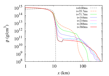
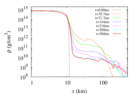
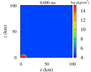
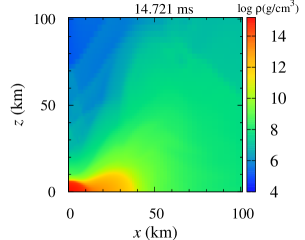
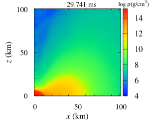
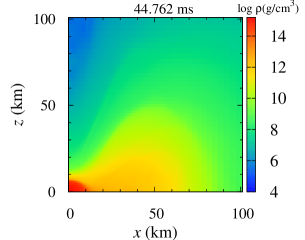
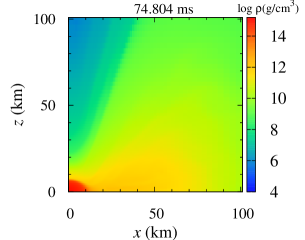
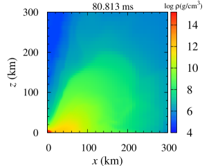
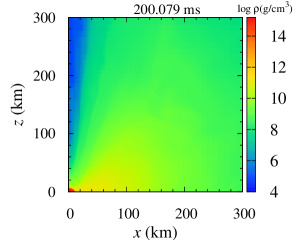
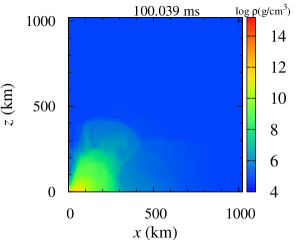
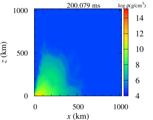
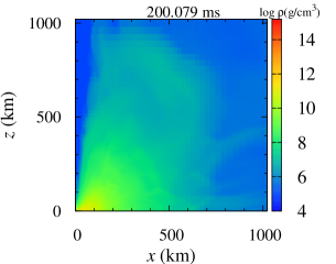
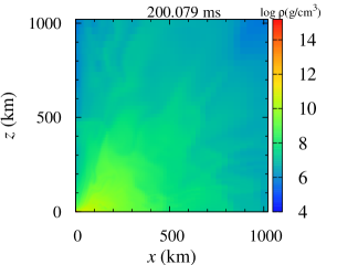
Figure 3 displays the evolution of density profiles on the equatorial plane for and 0.03. Figure 4 also displays the evolution of density profiles on the - plane for . These figures show that in a short time scale after the onset of the simulations, dense tori with the maximum density are formed around the neutron stars. As Figs. 3 and 4 show, the density of the tori subsequently decreases with time due to a long-term viscous process. Specifically, matter expands outward by the viscous heating and angular-momentum transport (see Fig. 4 and discussion below). These figures indicate that the viscous braking of the neutron-star rotation should continue as long as the dense envelope and torus surrounding it presents (for a time scale of ms)). The right panel of Fig. 2 also shows that the spin-down rate of the neutron star depends only weakly on the grid resolution.
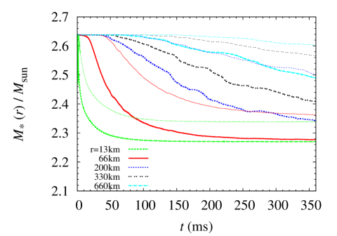
Because of the long-term angular-momentum transport, a dense and massive torus surrounding the central neutron star is evolved: see Fig. 4. The neutron-star mass decreases (torus mass increases) gradually with time. Figure 5 displays the rest mass contained in given radii as functions of time for (thin curves) and 0.03 (thick curves). The chosen radii are 13, 66, 200, 330, and 660 km (dashed, solid, dotted, dot-dot, and dash-dot curves). Up to ms, the matter is ejected from the central neutron star and constitutes a torus, and for ms, the rest mass of the neutron star is approximately fixed (see the dashed curves labeled by km). At ms, the neutron-star rest mass, defined by the rest mass for , is reduced to 89% and 85% of the total rest mass for and 0.03, respectively.
The torus mass should depend on the initial profile of the angular velocity and the compactness of the neutron star. Since we knew that tori of such high mass and high density are often formed around the massive neutron star in the simulations of binary neutron star mergers STU2005 ; Hotokezaka2013 , in the present work, we chose the initial condition that could form the object similar to the merger remnant of binary neutron stars.
After the formation of the torus, the matter in the torus expands outward. This is found from Fig. 5: Differences between the dashed curves of km and any other curves decrease with time; e.g, for , by comparing the curves of and 66 km, we find that the mass of the inner part of the torus is at ms and it decreases to at ms.
The matter of the torus on the equatorial plane has nearly Keplerian motion (see the left panel of Fig. 2). Thus, in the outer envelope of the neutron star and in particular in the torus, differential rotation remains, and hence, viscous angular momentum transport continuously works in the outer part of the system. Consequently, the viscous heating plays an important role even after the neutron star settles to a rigidly rotating state. The time scale for this process should be much longer than the viscous time scale in the differentially rotating neutron star, because the values of and are larger in the outer part than the inner part (see Eq. (58) for the definition of the viscous time scale, ).
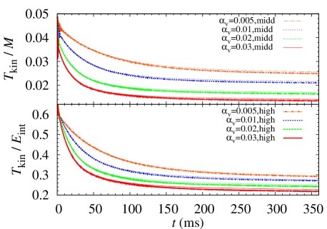
Figure 6 plots the evolution of total kinetic energy and the ratio of the total kinetic energy to total internal energy as functions of time. Due to the continuous viscous process, the kinetic energy is dissipated and converted to the internal energy. For –0.03, the kinetic energy is decreased by –70% until ms. Here, the dissipation rate of the kinetic energy is higher for the larger value of . The ratio of the kinetic to internal energy decreases in a similar manner to that for the kinetic energy, i.e., the increase rate of the internal energy is much lower than the decrease rate of the kinetic energy. Our interpretation for this is that the increase of the internal energy resulting from the viscous dissipation is consumed by the adiabatic expansion of the torus, as Fig. 4 indicates this fact.
Since no cooling effect except for the adiabatic expansion is taken into account in this study (although we conservatively include the shock-heating effect by choosing a small value of ), the geometrical thickness of the torus is monotonically increased by the viscous heating. We note that in the presence of a rapidly rotating neutron star at center (in the absence of a black hole that absorb matter), torus matter cannot efficiently fall onto the neutron star. Thus, unless the torus matter is ejected outwards, it continuously contributes to the viscous heating and resulting increase of its geometrical thickness. In reality, the neutrino emission would come into play for this type of the dense system. The typical neutrino cooling time scale may be longer than the viscous heating time scale of ms for the region of the density larger than because neutrinos are optically thick and trapped in the torus trap . However, after the torus expands and its density is decreased, subsequent expansion may be prohibited by the neutrino cooling. On the other hand, neutrino irradiation may enhance the torus expansion and mass ejection because the torus and outer part of the neutron star are quite hot and can be strong neutrino emitters. Incorporating the neutrino physics is one of the issues planned for our future work.
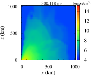
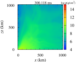
As a result of the monotonic increase of the geometrical thickness of the torus, a funnel structure is eventually formed (see the bottom panels of Fig. 4). Figure 7 displays snapshots of the density profiles for a wide region of 1000 kmk̇m at , 200, and 300 ms for (left), 0.01 (middle), and 0.03 (right), respectively. Vertically expanding matter is clearly found in this figure. This is very similar to and qualitatively the same as the structure found in MHD simulations in general relativity (e.g., Refs. Hawley2006 ; kiuchi2015 ). This agreement is reasonable because in both cases, viscous or MHD shock heating enhances the geometrical thickness, and thus, the rotating matter expands in the vertical direction. This result suggests that viscous hydrodynamics would capture an important part of the MHD effects such as shock heating and subsequent torus evolution at least qualitatively.
Due to the continuous viscous heating in the outer part of the neutron star and surrounding torus, a part of matter of the torus is outflowed eventually. Figure 8 displays the rest mass of the outflowed and ejected matter, and , and the averaged velocity of the ejecta as functions of time. Here, the outflowed component is estimated from the rest-mass and energy fluxes for a coordinate sphere at km, and if the specific energy for a fluid component becomes positive, i.e., , we specify it as the ejecta component. The averaged velocity of the ejecta is defined by where is the kinetic energy of ejecta; a fraction of that satisfies . We note that the curves for with different grid resolutions, in general, do not agree well with each other (this is in particular the case for small values of for which the ejecta mass is small). Our interpretation for this is that during the outflow is driven, there are many fluid components which are marginally unbound with , and hence, it is not feasible to accurately specify the ejecta components. However, the final values of the ejecta mass and kinetic energy depend weakly on the grid resolutions: These values are determined within a factor of .
The upper panel of Fig. 8 shows that irrespective of the values of , a fraction of the matter goes away from the central region. This is reasonable because geometrical thickness of the torus surrounding the central neutron star always grows irrespective of (see Fig. 7). The total amount of the outflowed mass is larger for the larger values of for a given moment of time, because the viscous heating rate is higher.
The outflow component comes primarily from the matter originally located at the torus, as we already mentioned (see Fig. 5). Figure 8 indicates that the outflowed mass eventually converges to a relaxed value for and 0.03. This is because the mass of the torus surrounding the central neutron star decreases with time as mentioned already. Thus, the final outcome after the evolution of differentially rotating neutron stars is likely to be a rigidly rotating neutron star surrounded by a low-density torus and a widely-spread envelope as Fig. 7 indicates.
Figure 8 shows that for , the total mass of the ejecta is . This value is approximately equal to or larger than those in the dynamical mass ejection of binary neutron star mergers, for which the typical ejecta mass is – hotoke13 . Thus, the long-term viscous mass ejection from the merger remnant may be the dominant mechanism of the mass ejection (see, e.g., Refs. Fer ; Perego2014 ; Just2014 for similar suggestions). On the other hand, for and 0.01, the ejecta mass is of order and , respectively: Only a small fraction of the outflow material can be ejecta. This indicates that to get a large value of the ejecta mass by the viscous process, an efficient viscous heating would be necessary (in reality, strong MHD turbulence would be necessary).
The bottom panel of Fig. 8 shows that the averaged velocity of the ejecta is irrespective of the values of . This is smaller than that for the dynamical mass ejection hotoke13 but the result is consistent with other viscous hydrodynamics results (see, e.g., Ref. Fer ). As discussed in Sec. I, rotating massive neutron stars surrounded by a massive torus are likely to be canonical outcomes of the binary neutron star merger. During the binary merger, the matter would be dynamically ejected, in particular, at the onset of the merger with the typical averaged velocity hotoke13 . If the remnant massive neutron stars are long-lived, they may subsequently eject the matter by the viscous effect. As suggested in this paper, the averaged velocity for it would be less than half of the velocity of the dynamical ejecta. Therefore, the viscous ejecta will never catch up with the dynamical ejecta: The ejecta are composed of two different components. In the binary neutron star mergers, the dynamical ejecta are likely to have a quasi-spherical or weakly spheroidal morphology hotoke13 . Thus, the viscous ejecta are likely to be surrounded by the dynamical ejecta.
As described in Refs. Li98 ; kasen13 , in the viscous ejecta as well as in the dynamical ejecta, r-process nucleosynthesis is likely to proceed because the ejecta are dense and neutron-rich, and then the ejecta will emit high-luminosity electromagnetic signals fueled by the radioactive decay of the unstable r-process heavy elements. In the presence of strong viscous wind, there may be two components in the light curve, while in its absence, the dynamical ejecta would be the primary source for the electromagnetic signals kasen15 . As Kasen and his collaborators illustrate, the shape of the light curve is quite different depending on the presence or the absence of the viscous wind. Our present result indicates that the viscous ejecta would be surrounded by the quasi-spherical dynamical ejecta. This suggests that the emission from the viscous ejecta could be absorbed by the dynamical ejecta, and then, the absorbed energy could be reprocessed and power up the emissivity of the dynamical ejecta.
The electromagnetic signal associated with the decay of unstable r-process elements is one of the most promising electromagnetic counterparts of the binary neutron star mergers. For the detection of these electromagnetic counterparts, we need a theoretical prediction as accurately as possible. The present study suggests that the light curve of this electromagnetic signal is uncertain due to the uncertainty of the viscous parameter that determines the ejecta mass. This implies that for the prediction of the electromagnetic signals, we have to perform numerical simulations taking into account a wide variety of the possibilities for the viscous parameter. Ultimately, we will need to perform a sufficiently high-resolution MHD simulation with no symmetry that can uniquely clarify the evolution of the differentially rotating merger remnants in the first-principle manner.
IV Summary
Employing a simplified version of the Israel-Stewart formulation for general relativistic viscous hydrodynamics that can minimally capture the effects of the viscous angular momentum transport and the viscous heating, we successfully performed axisymmetric numerical-relativity simulations for the evolution of a differentially rotating neutron star, which results in an approximately rigidly rotating neutron star surrounded by a massive torus. The detailed evolution process of this model with a sufficiently high viscous parameter is summarized as follows. First, by the outward angular momentum transport process, the initially differential rotation state is forced to be an approximately rigid rotation state in the inner region of the neutron star. At the same time, the torus with substantial mass is formed due to the viscous angular momentum transport from the neutron star. The time scale for this early evolution is quite short ms (i.e., the viscous time scale of the differentially rotating neutron star). The outcome in this stage is similar to the merger remnant of binary neutron stars.
Subsequently, the torus mass (including envelope surrounding the torus) increases spending a long time scale ms and eventually reaches – in the present model (this mass should depend on the initial choice of the models). After the formation of the system composed of a (approximately) rigidly rotating neutron star and a differentially rotating massive torus, the viscous effect still plays an important role near the outer surface of the neutron star and in the torus. Due to the subsequent long-term viscous heating effect there, the thermal pressure of the torus is increased, and as a result, the geometrical thickness of the torus monotonically increases. Also, the torus gradually expands along the equatorial direction because of the viscous angular momentum transport. For a sufficiently high viscous parameter, eventually, a strong outflow is driven from the torus. The ejecta mass can reach for in our model. Therefore, if a viscous process is efficient for the remnant of binary neutron star mergers, it is natural to expect the ejecta of large mass that is comparable to or larger than the mass of the dynamical component ejected during the merger phase. Since its velocity is likely to be smaller than , the viscous-driven ejecta will be surrounded by the dynamical ejecta for which the typical velocity is .
As we discussed in Sec. I, the remnants of binary neutron star mergers are in general differentially rotating objects (typically a massive neutron star surrounded by a torus), which would be evolved by MHD turbulence. Thus, in reality, the evolution of the merger remnants should be determined by the MHD processes, and for clarifying it, we have to perform a high-resolution non-axisymmetric MHD simulation in general relativity, for which the resolution has to be higher than the current best one kiuchi . As we showed in this paper, if the effective viscous parameter, , is larger than a critical value, a substantial amount of matter would be ejected from the merger remnant. Even for the case that is smaller than the critical value, a large amount of matter could expand to a region far from the central merger remnant. Thus, the picture for the evolution of the merger remnant could be significantly different from that in the absence of the MHD effects. A future high-resolution MHD simulation is awaited for precisely understanding the evolution process of the merger remnant. However, in the near future, such simulations cannot be done because of the restricted computational resources. The second-best strategy for exploring the mass ejection process from the merger remnant will be to perform a detailed viscous hydrodynamics simulation systematically changing the viscous parameter in a plausible range.
Note added in proof: After we submitted this paper, a paper by David Radice radice was submitted to arXiv. He describes another viscous hydrodynamics formalism that works well. Although he focuses only on the case with a small viscous parameter (in the terminology of alpha viscosity, he focuses only on the cases of or less), we find that his results agree qualitatively with our findings.
Acknowledgements.
We thank S. Inutsuka and L. Lehner for helpful discussion on general-relativistic viscous hydrodynamics. This work was supported by Grant-in-Aid for Scientific Research (Grant Nos. 24244028, 15H00782, 15H00783, 15H00836, 15K05077, 16H02183, 16K17706) of Japanese JSPS and by a post-K computer project (Priority issue No. 9) of Japanese MEXT.Appendix A Black hole and torus: Test simulation
In this appendix, we show results of a test simulation for the system composed of a black hole and a massive torus following the request by our referee who asks us to demonstrate more evidence that our formalism is capable of performing a long-term viscous hydrodynamics simulation. The purpose of this appendix is to demonstrate that our formalism indeed enables to perform simulations for strongly self-gravitating systems. More detailed study for the black hole-torus systems will be presented in a future work.
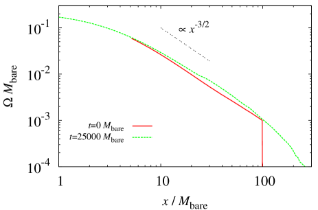
For this simulation, we prepare an equilibrium state composed of a black hole and a massive torus as the initial condition using the method of Ref. shibata07 . For this equilibrium state, we employ a non-rotating black hole with the puncture mass surrounded by a massive torus with the rest mass . The initial black-hole mass measured by the area of the black-hole horizon is . We note that the initial black hole mass is slightly different from because of the presence of the massive torus. The torus is modeled by the polytropic equation of state and during the simulation, we employ as the equation of state. Following Ref. kiuchi11 , we determine the specific angular momentum of the torus by providing the relation of where and are the specific angular momentum and angular velocity, respectively. Note that for with , the velocity profile approaches the Keplerian. With our choice of , the velocity profile looks close to the Keplerian (see Fig. 9). The inner and outer edges of the torus are set to be and (see the first panel of Fig. 10) . In the following, we employ a unit in which for showing the density.
In reality, the system with such massive torus would be unstable to non-axisymmetric instability like the Papaloizou-Pringle instability PP84 , even though the angular velocity profile is far from that of the const law. The purpose of this test simulation is to confirm that our viscous hydrodynamics formalism enables us to perform a long-term stable simulation for this self-gravitating system. Hence, disregarding the non-axisymmetric instability, we perform an axisymmetric simulation.


In this test simulation, we set where we choose , , : We employ a high value of to accelerate the evolution. The set up of the computational domain is as follows: , , and (see Sec III A for these quantities). The outer boundary along each axis is located at .
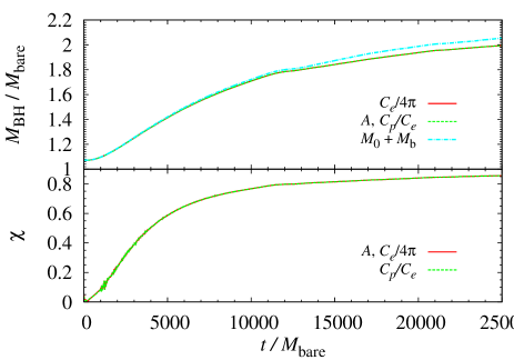
During the viscous hydrodynamics process, angular momentum transport actively works in the torus, and as a result, a part of the matter of the torus falls into the black hole. Then, the mass and spin of the black hole increase monotonically until the spin parameter reaches a sufficiently high value. After the high-spin state is reached, the evolution speed of the black hole is decelerated because the specific angular momentum at the innermost stable circular orbit around the high-spin black hole becomes lower than the values of most of the torus matter and the infalling of the matter into the black hole is suppressed. In this test simulation, we follow the evolution of the system until the dimensionless spin, , is relaxed to be (see Fig. 11).
For the analysis of this process, we have to determine the mass and spin of the black hole. Using the methods described in Ref. shibata07 , we analyze the quantities of the apparent horizons of the black hole. First, assuming that the black hole has the same properties as Kerr black holes even in the case that it is surrounded by the matter, the mass of the black hole is determined by
| (59) |
where is the equatorial circumferential length of horizons and is the irreducible mass of the black hole which is determined from the area of apparent horizons by . We will describe the method to determine in the next paragraph. Note that all the geometrical quantities are determined for the apparent horizons. We remark that for Kerr black holes, is satisfied. We also approximately estimate the mass of the black hole by summing up the total rest mass of the matter swallowed by the black hole, , and the initial black hole mass, . This approximate mass of the black hole is referred to as in the following. We note that the energy of the matter swallowed by the black hole would be smaller than because of the presence of the gravitational binding energy, and hence, would slightly overestimate the black hole mass (as shown in Fig. 11).
We determine by two methods. In the first method, we measure which is a monotonically decreasing function of . Here is the meridian circumferential length of horizons. Using the value of determined by this method, we subsequently determine shown in Eq. (59). In the second method, we use the relation of for determining the value of .
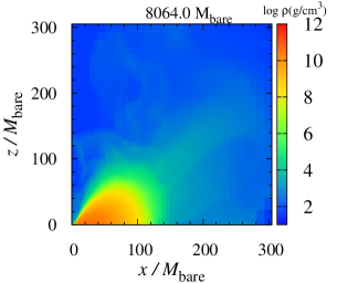
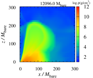
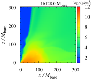
Figure 10 displays the evolution of the density profile of the torus. Due to the angular momentum transport inside the torus, a part of the matter falls into the black hole and another part of the matter expands outwards (second and third panels of Fig. 10). By the long-term viscous heating effect, the inner part of the torus is heated up significantly, in particular, a high-spin state with is reached (fourth panel of Fig. 10), and then, it expands to a vertical direction. By this outflow, a part of the torus matter is ejected from the system (fifth panel of Fig. 10). Eventually, a funnel structure is formed along the rotation axis of the black hole (sixth panel of Fig. 10). In this final stage of the evolution, the dimensionless black hole spin is (see Fig. 11).
Figure 11 plots the evolution of the mass and dimensionless spin of the black hole. We note that for , the accuracy for the determination of is not very good because the values of and are close to unity irrespective of the value of .
Besides such an early phase of the evolution, it appears that the quantities of the black hole are determined accurately because two independent methods for determining the mass and spin give approximately the same values. In addition, agrees approximately with the black hole mass determined by two methods. It is also reasonable that is slightly larger than and .
It is found that by the viscous accretion process, the system eventually relaxes to a system of a rapidly rotating black hole surrounded by a geometrically thick accretion torus. Such outcome is often found in general relativistic MHD simulations (e.g., Refs. Hawley2006 ; kiuchi2015 ). Our viscous hydrodynamics simulation captures such feature.
References
- (1) P. B. Demorest et al., Nature (London) 467, 1081 (2010); J. Antoniadis et al., Science 340, 1233232 (2013).
- (2) M. Shibata, K. Taniguchi, and K. Uryū, Phys. Rev. D 71, 084021 (2005): M. Shibata and K. Taniguchi, Phys. Rev D 73, 064027 (2006).
- (3) K. Hotokezaka, K. Kyutoku, H. Okawa, M. Shibata, and K. Kiuchi, Phys. Rev. D 83, 124008 (2011); K. Hotokezaka, K. Kiuchi, K. Kyutoku, T. Muranushi, Y. -I. Sekiguchi, M. Shibata and K. Taniguchi, Phys. Rev. D 88, 044026 (2013); K. Takami, L. Rezzolla, and L. Baiotti, Phys. Rev. D 91, 064001 (2015); T. Dietrich, S. Bernuzzi, M. Ujevic, and B. Brügmann, Phys. Rev. D 91, 124041 (2015).
- (4) D. J. Price and S. Rosswog, Science 312, 719 (2006).
- (5) K. Kiuchi, K. Kyutoku, Y. Sekiguchi, M. Shibata, and T. Wada, Phys. Rev. D 90, 041502(R) (2014); K. Kiuchi, P. Cerda-Duran, K. Kyutoku, Y. Sekiguchi, and M. Shibata, Phys. Rev. D 92, 124034 (2015).
- (6) S. A. Balbus and J. F. Hawley, Rev. Mod. Phys. 70, 1 (1998).
- (7) J. F. Hawley, S. A. Richers, X. Guan, and J. H. Krolik, Astrophys. J. 772, 102 (2013).
- (8) T. K. Suzuki and S. Inutsuka, Astrophys. J. 784, 121 (2014).
- (9) J. M. Shi, J. M. Stone, and C. X. Huang, Mon. Not. R. Soc. Astron. 456, 2273 (2016): G. Salvesen, J. B. Simon, P. J. Armitage, and M. C. Begelman, Mon. Not. R. Soc. Astron. 457, 8578 (2016).
- (10) J. Guilet, A. Bauswein, O. Just, and H.-T. Janka, arXiv: 1610.08532.
- (11) H. K. Moffatt, Magnetic Field Generation in Electrically Conducting Fluids (Cambridge Univ. Press, Cambridge, 1978).
- (12) M. D. Duez, Y.-T. Liu, S. L. Shapiro, and B. C. Stephens, Phys. Rev. D 69, 104030 (2004).
- (13) L. D. Landau and E. M. Lifshitz, Fluid Mechanics (Peragamon Press, London, 1959).
- (14) W. Israel and J. M. Stewart, Ann. Phys. 118, 341 (1976).
- (15) W. A. Hiscock and L. Lindblom, Annals of Physics, 151, 466 (1983).
- (16) S. L. Shapiro and S. A. Teukolsky, Black holes, White dwarfs, and Neutron stars: the Physics of Compact Objects (Wiley, 1983), chapter 14.
- (17) M. Alcubierre, S. Brandt, B. Brügmann, D. Holz, E. Seidel, R. Takahashi, and J. Thornburg, Int. J. Mod. Phys. D 10, 273 (2001).
- (18) M. Shibata, Prog. Theor. Phys. 104, 325 (2000); M. Shibata, Phys. Rev. D 67, 024033 (2003).
- (19) M. Shibata and Y. Sekiguchi, Prog. Theor. Phys. 127, 535 (2012).
- (20) A. Kurganov and E. Tadmor, J. Comp. Phys. 160 (2000), 241.
- (21) M. Shibata and T. Nakamura, Phys. Rev. D 52, 5428(1995): T. W. Baumgarte and S. L. Shapiro, Phys. Rev. D 59, 024007(1998): M. Campanelli, C. O. Lousto, P. Marronetti, and Y. Zlochower, Phys. Rev. Lett. 96, 111101 (2006): J. G. Baker, J. Centrella, D.-I. Choi, M. Koppitz, and J. van Meter, Phys. Rev. Lett. 96, 111102 (2006).
- (22) M. Shibata, M. D. Duez, Y.-T. Liu, S. L. Shapiro, and B. C. Stephens, Phys. Rev. Lett. 96, 031102 (2006).
- (23) B. Bruëgmann, J. A. Gonzalez, M. Hannam, S. Husa, U. Sperhake, and W. Tichy, Phys. Rev. D 77, 024027 (2008).
- (24) S. Kato, J. Fukue, and S. Mineshige, Black-Hole Accretion Disks (Kyoto University Press, 1998).
- (25) K. Kohri and S. Mineshige, Astrophys. J. 577, 311 (2002); T. Di Matteo, R. Perna, and R. Narayan, Astrophys. J. 579, 706 (2002); W. H. Lee, E. Ramirez-Ruiz, and D. Page, Astrophys. J. 632, 421 (2005); S. Setiawan, M. Ruffert, and H.-Th. Janka, Astron. Astrophys. 458, 553 (2006); M. Shibata, Y. Sekiguchi, R. Takahashi, Prog. Theor. Phys. 118, 257 (2007).
- (26) J. F. Hawley and J. H. Krolik, Astrophys. J. 641, 103 (2006).
- (27) K. Kiuchi, Y. Sekiguchi, K. Kyutoku, M. Shibata, K. Taniguchi, and T. Wada, Phys. Rev. D 92, 064034 (2015).
- (28) K. Hotokezaka, K. Kiuchi, K. Kyutoku, H. Okawa, Y. Sekiguchi, M. Shibata, and K. Taniguchi, Phys. Rev. D 87, 024001 (2013): Y. Sekiguchi, K. Kiuchi, K. Kyutoku, and M. Shibata, Phys. Rev. D 91, 064059 (2015).
- (29) R. Fernández and B. Metzger, Mon. Not. Royal Astron. Soc. 435, 502 (2013);
- (30) A. Perego, S. Rosswog, R. Cabezon, O. Korobkin, R. Kaeppeli, A. Arcones, M. Liebendoerfer, Mon. Not. Royal Astron. Soc. 443, 3134 (2014).
- (31) O. Just, A. Bauswein, R. A. Pulpillo, S. Goriely, and H.-Th. Janka Mon. Not. Royal Astron. Soc. 448, 541 (2014).
- (32) L.-X. Li and B. Paczynski, Astrophys. J. 507, L59 (1998); B. D. Metzger et al., Mon. Not. R. Astron. Soc., 406, 2650 (2010).
- (33) D. Kasen, N. R. Badnell, and J. Barnes, Astrophys. J. 774, 25 (2013); J. Barnes and D. Kasen, Astrophys. J. 775, 18 (2013); M. Tanaka and K. Hotokezaka, Astrophys. J. 775, 113 (2013).
- (34) D. Kasen, R. Fernández, B. D. Metzger, Mon. Not. R. Astro. Soc. 450, 1777 (2015).
- (35) D. Radice, Astrophys. J. Lett. to be published (arXiv: 1703.02046).
- (36) M. Shibata, Phys. Rev. D 76, 064035 (2007).
- (37) K. Kiuchi, M. Shibata, P. J. Montero, and J. A. Font, Phys. Rev. Lett. 106, 251102 (2011).
- (38) J. C. B. Papaloizou and J. E. Pringle, Mon. Not. R. Astron. Soc. 721, 208 (1984).