Evolution of circular, non-equatorial orbits of Kerr black holes due to gravitational-wave emission: II. Inspiral trajectories and gravitational waveforms

Abstract

The inspiral of a “small” ($\mu\sim 1-100\,M_{\odot}$) compact body into a “large” ($M\sim 10^{5-7}\,M_{\odot}$) black hole is a key source of gravitational radiation for the space-based gravitational-wave observatory LISA. The waves from such inspirals will probe the extreme strong-field nature of the Kerr metric. In this paper, I investigate the properties of a restricted family of such inspirals (the inspiral of circular, inclined orbits) with an eye toward understanding observable properties of the gravitational waves that they generate. Using results previously presented to calculate the effects of radiation reaction, I assemble the inspiral trajectories (assuming that radiation reacts adiabatically, so that over short timescales the trajectory is approximately geodesic) and calculate the wave generated as the compact body spirals in. I do this analysis for several black hole spins, sampling a range that should be indicative of what spins we will encounter in nature. The spin has a very strong impact on the waveform. In particular, when the hole rotates very rapidly, tidal coupling between the inspiraling body and the event horizon has a very strong influence on the inspiral time scale, which in turn has a big impact on the gravitational wave phasing. The gravitational waves themselves are very usefully described as “multi-voice chirps”: the wave is a sum of “voices”, each corresponding to a different harmonic of the fundamental orbital frequencies. Each voice has a rather simple phase evolution. Searching for extreme mass ratio inspirals voice-by-voice may be more effective than searching for the summed waveform all at once.

I Introduction

One of the goals of the space-based gravitational-wave detector LISA [1] is to make measurements that will probe gravity in the very strong field. The most stringent probes will involve binary black hole systems. Mergers of comparable mass black holes will be detectable throughout most of the universe [2]; their measurements will probe the violent dynamics of two black holes combining to form a single hole. LISA will measure hundreds to thousands of wave cycles in such events, probing their waveforms with moderate precision. When the mass ratio of the system is extreme ($M_{1}/M_{2}\simeq 10^{-3}-10^{-7}$), measurement of the waves probes the quiescent structure of the Kerr black hole spacetime. LISA should measure tens of thousands to millions of cycles from such inspirals (depending mostly on mass ratio), and thus may be able to measure their waves — and probe black hole spacetimes — with extremely high precision. Extreme mass ratio inspirals will be the focus of this analysis.

The case for studying extreme mass ratio inspirals has been argued at length elsewhere; I refer the reader to the Introductions of Refs. [2] and [3] for detailed discussion. Briefly, detailed studies [4, 5] have shown that compact stellar remnants in the central cusp of galaxies are scattered into very tight, eccentric orbits of the galaxies’ black hole at a rate of at least several events per year out to a Gigaparsec (perhaps as high as an event per month). The final year or so of inspiral (depending on the large black hole’s mass and spin, and on the binary’s mass ratio) will occur as the small body spirals through the most extreme strong-field region of the black hole spacetime, from several horizon radii down to orbits just outside the hole’s event horizon.

By tracking the phase evolution of the waves over the many cycles radiated in this year, it should be possible to measure strong-field characteristics of the black hole spacetime. Fintan Ryan [8] has shown that these waves can be used to reconstruct the multipolar structure of the black hole. By the “no hair” theorem, a Kerr black hole’s multipole moments are uniquely determined by its mass $M$ and spin $a$. Measuring more than two moments tests whether the massive object at the core of a galaxy is a black hole, or whether it is some more exotic compact object, such as a soliton star.

Analyzing how well one can measure the multipoles of a massive compact object in this manner means computing gravitational waves from the inspiral of realistic small bodies on inclined, eccentric trajectories about bodies with arbitrary multipole moments. We are rather far from being able to analyze such a system. For now, I require that the massive body be a black hole — this greatly simplifies the description of its orbits. I also take the inspiraling body to be pointlike and nonspinning, sidestepping issues of spin-spin and spin-orbit coupling which complicate the inspiral and may in fact lead to chaos [9, 10]. Finally, because rigorous strong-field radiation reaction is currently being developed [11], I use a “poor man’s radiation reaction” approach, balancing the flux of energy and angular momentum in gravitational waves with the change in orbital energy and angular momentum. This formalism works well if the inspiral is adiabatic: the change in orbital parameters due to wave emission must be slow. (A more precise definition of adiabatic and “slow” is given in Sec. II B.) At present, the flux-balance approach cannot be used to find the change in the third constant of Kerr orbits (the Carter constant $Q$), so I require that the orbit be initially “circular” (of constant Boyer-Lindquist radius). These orbits do not become eccentric under adiabatic radiation reaction [12, 13, 14], constraining the system enough that $Q$’s evolution can be inferred from the changes in the orbital energy and angular momentum alone.

Given the large number of restrictions imposed, it is clear this analysis is rather far from the ultimate goal of laying the foundations for compact body multipole measurement with LISA. However, it is sufficient to begin developing gravitational waveforms and probing the inspiral trajectories for non-trivial orbits. These orbits are colored rather strongly by the orbital frequencies and their harmonics, and, despite the numerous restrictions, have a fairly ornate structure. This analysis is a useful way to produce gravitational waveforms that have a character similar to what we are likely to observe with LISA. They are restricted enough that they can be calculated with tools available now, but have enough structure that they can be used for developing data analysis tools and understanding how measurement of extreme mass ratio inspirals with LISA will work in practice.

In the remainder of the Introduction, I summarize the structure and results of the paper. I first review the properties of circular, inclined orbits of Kerr black holes and the radiation reaction formalism used here. This material is presented in far greater detail in Refs. [6] and [16]. This paper just presents equations and points the reader to the relevant literature for a detailed derivation. In the end, radiation reaction data are presented as vectors $(\dot{r},\dot{\iota})$ living at orbital coordinates $(r,\iota)$. These vectors describe how radiation drives the body to spiral through a sequence of orbits into the hole. The wave itself is developed from a set of complex amplitudes $Z^{H}_{lmk}$ which constitute a multipole expansion of the gravitational-wave strain measured by distant observers. This fully sets up this analysis.

Inspiral trajectories are constructed by beginning at some coordinate $(r_{0},\iota_{0})$ and stepping inward along the data $(\dot{r},\dot{\iota})$ until the body hits the last dynamically stable orbit and plunges into the hole. The data are actually computed on a grid that covers the parameter space of allowed orbits deep in the strong field, and are interpolated to get radiative effects off the grid. Section III A first describes how the data grid is set up, as well as which data are stored on it. Section III B then briefly describes how the integration is done.

Results are given in Secs. IV and V. First I discuss the inspiral trajectories in Sec. IV; they and their various features are displayed for several choices of black hole spin in Figs. 2, 3, 5, 6, and 7. During inspiral lasting 1–2 years, the inspiraling body executes several hundred thousand orbits in the extreme strong field of the massive black hole. This is not a surprise, and has of course been known for quite some time. More interestingly, the inclination angle barely changes during inspiral, particularly when spin $a\lesssim 0.8M$. This gives further credence to a suggestion by Curt Cutler that it would be worthwhile to explore “faking” the inspiral of generic Kerr orbits by holding the inclination angle fixed — this would fix the change in the Carter constant provided the changes in $E$ and $L_{z}$ were known.

The influence of the black hole’s event horizon on the inspiral is very strong. A very useful way to understand this effect is that the inspiraling body tidally distorts the black hole, causing the horizon to bulge. This bulge then exerts a torque back on the body. This viewpoint is explained at a very pedagogically accessible level in Chapter VII of Ref. [17], which in turn is based on the work of Hawking and Hartle [18] and Hartle [19]. If the hole is rapidly rotating, this torque tends to significantly slow the inspiral, transferring some of the hole’s rotational kinetic energy to the orbital motion. Inspiral can be prolonged for several weeks ($\sim 5\%$ of the total inspiral time) by this effect, adding tens of thousands of additional orbits. By contrast, if the hole is rotating slowly, the torque exerted by the horizon bulge speeds up the inspiral. This fascinating coupling of the horizon to the inspiraling body’s dynamics is an example of how strong-field features of the Kerr spacetime can be seen in gravitational waves.

Section V discusses the waves produced as the body spirals inward. It should be strongly emphasized that computing waveforms is more difficult than computing inspiral trajectories. The waveforms require both the magnitude and phase of the complex amplitudes $Z^{H}_{lmk}$ to high precision; the trajectories require just the magnitude. As such, the results shown in Sec. V should be taken as an important first step in generating extreme mass ratio inspiral waves, but can — and should! — be improved dramatically.

Multiple harmonics of the orbital frequencies $\Omega_{\phi}$ and $\Omega_{\theta}$ are very important; cf. Fig. 8. Following a suggestion of Sam Finn, I write the waveform as a sum over many “voices”: $h(t)=\sum h_{lmk}(t)$. Each voice $h_{lmk}(t)$ corresponds to a particular harmonic of the orbital frequencies, and has its own amplitude and phase evolution. Writing the waveform in this manner emphasizes that the phase evolution of each voice is rather simple, though the sum may be complicated and difficult to follow. It is likely this multi-voice structure will carry over to the generic case, adding an additional index for harmonics of the radial frequency $\Omega_{r}$. The analysis of LISA data may be facilitated by searching for extreme mass ratio inspirals voice-by-voice, rather than searching for the “chorus” of all voices at the same time. Concluding discussion, including suggestions for future work and extensions to this analysis, is given in Sec. VI.

Throughout this paper, an overdot denotes $d/dt$, and a prime denotes $\partial/\partial r$. An overbar indicates complex conjugation. The quantities $t$, $r$, $\theta$, and $\phi$ refer to the Boyer-Lindquist coordinates. I use units with $G=1=c$ throughout.

II Review: Circular orbits and radiation reaction

A Geodesic orbits

Orbits of Kerr black holes are specified by choosing their energy $E$, axial angular momentum $L_{z}$, and Carter constant $Q$. The values used here have been divided by the small body’s mass $\mu$ ($E$ and $L_{z}$) or $\mu^{2}$ ($Q$) and are thus the specific energy, angular momentum and Carter constant. Having chosen these constants (and initial conditions), the orbit is then governed by geodesic equations for the small body’s Boyer-Lindquist coordinates ($t$, $r$, $\theta$, $\phi$) as a function of proper time $\tau$ measured along its worldline; see [20].

To describe circular orbits, it is useful to introduce the function $R\equiv\Sigma^{2}(dr/d\tau)^{2}$:

$$R=\left[E(r^{2}+a^{2})-aL_{z}\right]^{2}-\Delta\left[r^{2}+(L_{z}-aE)^{2}+Q\right]\;.$$ (1)

(The function $\Sigma=r^{2}+a^{2}\cos^{2}\theta$, and $\Delta=r^{2}-2Mr+a^{2}$.) Circular orbits satisfy $R=0$ and $R^{\prime}=0$; stable circular orbits satisfy in addition $R^{\prime\prime}\leq 0$. Given the radius $r$ and one of the three constants $E$, $L_{z}$, or $Q$, it is straightforward to solve the system $R=0$, $R^{\prime}=0$ for the other two. In this paper, I choose $r$ and $E$ and then solve for $L_{z}$ and $Q$:

$$L_{z}(r,E) = {EM(r^{2}-a^{2})-\Delta\sqrt{r^{2}(E^{2}-1)+rM}\over a(r-M)}\;,$$ (2)

$$Q(r,E) = {\left[(a^{2}+r^{2})E-aL_{z}(r,E)\right]\over\Delta}-\left[r^{2}+a^{2}E^{2}-2aEL_{z}(r,E)+L_{z}(r,E)^{2}\right]\;.$$ (3)

[Note that in Ref. [16], the $a^{2}E^{2}$ inside the second set of square brackets is incorrectly written $a^{2}E$.]

At a given radius, two orbits bound the behavior of all stable circular orbits. The most-bound orbit is the prograde equatorial orbit ($\iota=0$). Its constants are [21]

$$E^{\rm mb} = {{1-2v^{2}+qv^{3}}\over\sqrt{1-3v^{2}+2qv^{3}}}\;,$$ (4)

$$L_{z}^{\rm mb} = rv{{1-2qv^{3}+q^{2}v^{4}}\over\sqrt{1-3v^{2}+2qv^{3}}}\;,$$ (5)

$$Q^{\rm mb} = 0\;,$$ (6)

where $v\equiv\sqrt{M/r}$ and $q\equiv a/M$. Prograde equatorial orbits exist at all radii outside $r_{\rm pro}$, where

$$r_{\rm pro}/M = 3+Z_{2}+\left[(3-Z_{1})(3+Z_{1}+2Z_{2})\right]^{1/2}\;,$$ (7)

$$Z_{1} = 1+\left[1-(a/M)^{2}\right]^{1/3}\left[(1+a/M)^{1/3}+(1-a/M)^{1/3}\right]\;,$$ (8)

$$Z_{2} = \left[3(a/M)^{2}+Z_{1}^{2}\right]^{1/2}\;.$$ (9)

This is also the radius of the LSO when $\iota=0^{\circ}$ — no stable circular orbits exist inside $r_{\rm pro}$. If $r<r_{\rm ret}$, where

$$r_{\rm ret}/M=3+Z_{2}+\left[(3-Z_{1})(3+Z_{1}+2Z_{2})\right]^{1/2}\;,$$ (10)

then the least-bound orbit is on the LSO, and the constants $(E^{\rm lb},L_{z}^{\rm lb},Q^{\rm lb})$ are found by numerically solving the system of equations $R=0$, $R^{\prime}=0$, $R^{\prime\prime}=0$. If $r>r_{\rm ret}$, the least-bound orbit is the retrograde equatorial orbit ($\iota=180^{\circ}$), and its constants are

$$E^{\rm lb} = {{1-2v^{2}-qv^{3}}\over\sqrt{1-3v^{2}-2qv^{3}}}\;,$$ (11)

$$L_{z}^{\rm lb} = -rv{{1+2qv^{3}+q^{2}v^{4}}\over\sqrt{1-3v^{2}-2qv^{3}}}\;,$$ (12)

$$Q^{\rm lb} = 0\;.$$ (13)

Orbits with $Q\neq 0$ are inclined with respect to the equatorial plane; a useful definition of the inclination angle $\iota$ is

$$\cos\iota={L_{z}\over\sqrt{L_{z}^{2}+Q}}\;.$$ (14)

Mapping out all stable circular orbits at some radius is fairly straightforward. First, calculate the constants that describe the most-bound orbit [Eqs. (4)–(6)]. Second, calculate the constants for the least-bound orbit [solving the system $R=0$, $R^{\prime}=0$, $R^{\prime\prime}=0$ if $r<r_{\rm ret}$; using Eqs. (11)–(13) otherwise]. Finally, vary $E$ from its most-bound to its least-bound extreme.

Circular orbits are periodic, with two (generally incommensurate) frequencies $\Omega_{\theta}$ and $\Omega_{\phi}$, related to the small body’s motion in the $\theta$ and $\phi$ coordinates. These two frequencies (and their harmonics) strongly stamp the gravitational waveform. Typically, $\Omega_{\phi}>\Omega_{\theta}$; the differences are due to the oblate geometry of a rotating black hole and frame dragging (which can greatly augment $\Omega_{\phi}$). A detailed derivation of these frequencies is given in Sec. IIC of Ref. [6].

B Radiative corrections

The radiation reaction formalism used here is based on the Teukolsky equation [7], which governs the evolution of the complex Weyl curvature scalar related to radiative perturbations, $\psi_{4}$. This section briefly outlines how the radiative corrections are computed, particularly the quantities relevant to this analysis. Reference [6] discusses this material in greater detail.

The “master equation” for the evolution of $\psi_{4}$ is separated with the multipolar decomposition [7]

$$\psi_{4}={1\over(r-ia\cos\theta)^{4}}\int_{-\infty}^{\infty}d\omega\sum_{lm}R_{lm\omega}(r)\,_{-2}S^{a\omega}_{lm}(\theta)e^{i(m\phi-\omega t)}\;.$$ (15)

The $t$ and $\phi$ dependences are trivial. The function ${}_{-2}S^{a\omega}_{lm}(\theta)$ is a spin-weighted spheroidal harmonic. It is useful for describing the $\theta$ dependence of a radiation field with spin weight $-2$ in an oblate geometry. An effective algorithm for calculating this function is given in Appendix A of Ref. [6].

Computing the radial function $R_{lm\omega}$ takes some effort. This function obeys the Teukolsky equation:

$$\Delta^{2}{d\over dr}\left({1\over\Delta}{dR_{lm\omega}\over dr}\right)-V(r)R_{lm\omega}=-{\cal T}_{lm\omega}(r)\;.$$ (16)

This equation is in self-adjoint form, and so can be solved with Green’s functions [23]. The homogeneous Teukolsky equation has two independent solutions, $R^{H}_{lm\omega}(r)$ (which obeys the boundary condition that radiation must be purely ingoing at the event horizon) and $R^{\infty}_{lm\omega}(r)$ (which obeys the condition that radiation must be purely outgoing at infinity). From these solutions and from the source function ${\cal T}_{lm\omega}(r)$, one can write down the general solution $R_{lm\omega}(r)$:

$$R_{lm\omega}(r)=Z^{H}_{lm\omega}R^{\infty}_{lm\omega}(r)+Z^{\infty}_{lm\omega}R^{H}_{lm\omega}(r)\;.$$ (17)

A detailed description of how one computes $Z_{lm\omega}^{H}$, $Z_{lm\omega}^{\infty}$, $R_{lm\omega}^{H}$, and $R_{lm\omega}^{\infty}$ (and how they relate to the source function ${\cal T}_{lm\omega}$) is given in Ref. [6]. The most important details for this paper are as follows. First, for circular orbits, the source and all quantities derived from it are describable as harmonics of $\Omega_{\theta}$ and $\Omega_{\phi}$. Defining $\omega_{mk}=m\Omega_{\phi}+k\Omega_{\theta}$, the functions $Z_{lm\omega}^{H}$ and $Z_{lm\omega}^{\infty}$ can be decomposed into harmonics:

$$Z^{H,\infty}_{lm\omega}=\sum_{k}Z^{H,\infty}_{lmk}\delta(\omega-\omega_{mk})\;.$$ (18)

Second, as $r\to r_{+}=M+\sqrt{M^{2}-a^{2}}$ (the coordinate of the event horizon), $Z_{lm\omega}^{H}\to 0$ and $Z_{lm\omega}^{\infty}\to\mbox{constant}$; as $r\to\infty$, $Z_{lm\omega}^{\infty}\to 0$ and $Z_{lm\omega}^{H}\to\mbox{constant}$. The behavior of the radiation at infinity thus depends only on $Z_{lmk}^{H}$, and at the horizon only on $Z_{lmk}^{\infty}$. The gravitational waveform is

$$h_{+}-ih_{\times}=\sum_{lmk}{Z^{H}_{lmk}\over\omega_{mk}^{2}}{{}_{-2}S}^{a\omega_{mk}}_{lm}(\vartheta)e^{i(m\varphi-\omega_{mk}t)}\;,$$ (19)

and the fluxes are

$$\left({dE\over dt}\right)_{\rm rad}^{\infty,H} = \sum_{lmk}\alpha_{lmk}^{\infty,H}{|Z^{H,\infty}_{lmk}|^{2}\over 4\pi\omega_{mk}^{2}}\;,$$ (20)

$$\left({dL_{z}\over dt}\right)_{\rm rad}^{\infty,H} = \sum_{lmk}\alpha_{lmk}^{\infty,H}{m|Z^{H,\infty}_{lmk}|^{2}\over 4\pi\omega_{mk}^{3}}\;.$$ (21)

By assumption, the change in the orbital energy and angular momentum is opposite in sign to that radiated: $\dot{E}^{\rm orbit}=-\dot{E}^{\rm rad}$, ${\dot{L}}_{z}^{\rm orbit}=-{\dot{L}}_{z}^{\rm rad}$. Note the somewhat confusing reversal of $H$ and $\infty$ on the $Z_{lmk}$ coefficients; this follows from the definition in Eq. (17). The factor $\alpha^{H}_{lmk}$ is a rather messy coefficient that follows from transforming the Kinnersley null tetrad (which is used to construct $\psi_{4}$ [24]) to the Hawking-Hartle null tetrad [18] (which is well behaved on the event horizon); see Ref. [6] for further details. (The factor $\alpha^{\infty}=1$; it is introduced so that these formulas can be written compactly.) As noted in [6], there is a symmetry relation between quantities at $(l,m,k)$ and $(l,-m,-k)$:

$$Z^{H,\infty}_{l-m-k}=(-1)^{l+k}{\bar{Z}}^{H,\infty}_{lmk}\;.$$ (22)

This relationship can be used to reduce computation time — compute half the multipoles, use symmetry to get the other half. Alternatively, it can be used to improve computational accuracy — compute all the multipoles, use symmetry to reduce error:

$$Z^{H,\infty}_{lmk}={1\over 2}\left[Z^{H,\infty}_{lmk;\,{\rm comp}}+(-1)^{l+k}{\bar{Z}}^{H,\infty}_{l-m-k;\,{\rm comp}}\right]\;.$$ (23)

This second approach was used here.

A large number of terms were included when evaluating Eq. (21). A detailed discussion of the truncation criterion used here is given in Sec. VA of Ref. [6]; in the language of that paper, $\epsilon_{k}=10^{-4}$ and $\epsilon_{l}=10^{-3}$. The truncation error in $\dot{E}^{H,\infty}$ and ${\dot{L}}_{z}^{H,\infty}$ is therefore roughly $10^{-3}$. Obtaining this level of accuracy required summing to at least $l=8$ (for innermost orbits of the $a=0.998M$ black hole, the sums were taken to $l=19$). For each value of $l$, between 10 and 30 values of $k$ were included. In all cases, the sum over $m$ ranged from $-l$ to $l$.

Using the Teukolsky equation to compute $\dot{E}^{H,\infty}$ and ${\dot{L}}_{z}^{H,\infty}$ requires that the inspiral be adiabatic: over orbital timescales, the trajectory must be nearly geodesic. This requirement enters through the source term, which depends on the inspiraling body’s worldline. This is potentially the setup for a Catch-22: we need the worldline in order to compute the body’s radiative corrections, but the corrections determine that worldline! The solution is to take the worldline to be geodesic for computing the source. We thus use the zeroth order (in $\mu/M$) geodesic motion to compute the first order radiative corrections. This is a good approximation only when the radiative change in any orbital quantity $\chi$ over an orbit is much less than $\chi$: $\dot{\chi}T_{\rm orb}\ll\chi$. Very useful quantities to monitor are the orbital frequencies, $\Omega_{\phi}$ and $\Omega_{\theta}$. Because $T_{\theta}=2\pi/\Omega_{\theta}$, and defining $T_{\phi}=2\pi/\Omega_{\phi}$, the adiabaticity condition for these quantities can be written

$${\cal N}_{\phi,\theta}\equiv{1\over 2\pi}{\Omega_{\phi,\theta}^{2}\over{\dot{\Omega}}_{\phi,\theta}}\gg 1\;,$$ (24)

These parameters are closely related to the number of accumulated orbits in $\phi$ and $\theta$:

$$N_{\phi,\theta}={1\over 2\pi}\int dt\,\Omega_{\phi,\theta}=\int d\ln\Omega_{\phi,\theta}\,{\cal N}_{\phi,\theta}\;.$$ (25)

The condition ${\cal N}_{\phi,\theta}\gg 1$ tells us that the orbits accumulated by the body as it passes through the orbital frequency band centered on $\Omega_{\phi,\theta}$ and of width $\delta\Omega_{\phi,\theta}=\Omega_{\phi,\theta}$ must be very large. More simply, the body must spend many orbits near any point in its orbital phase space.

The Teukolsky equation can only tell us about the changes in $E$ and $L_{z}$. To fully describe the small body’s spiral in, we impose circularity: adiabatic radiation reaction changes an orbit’s radius and inclination angle, but it does not make the orbit eccentric [12, 13, 14] — circular orbits remain circular. Imposing this rule gives a relatively simple relationship between ($\dot{Q},\dot{r}$) and ($\dot{E},{\dot{L}}_{z}$); see Ref. [6], Sec. IIIA for details. Once $\dot{Q}$ and ${\dot{L}}_{z}$ are known, it is simple to get the rate of change of $\iota$ using Eq. (14); cf. Eqs. (3.7) and (3.8) of Ref. [6]. The data $(\dot{r},\dot{\iota})$ are the foundation for all the inspiral trajectories discussed in the next section.

Letting $\chi$ stand for any of the quantities ($E,L_{z},Q,r$), the total change in $\chi$ is found by summing the change due to radiation flux out to infinity and due to radiation flux down the event horizon:

$$\dot{\chi}=\dot{\chi}^{\infty}+\eta\dot{\chi}^{H}\;.$$ (26)

The parameter $\eta$ (which clearly should equal 1) is introduced so that we can “turn off” the flux down the horizon. As we shall see later, setting $\eta=0$ is a very interesting test of how strongly the black hole’s event horizon influences inspiral.

III Computing inspiral trajectories and waveforms

Using the techniques described in Sec. II, it is straightforward to compute the inspiral trajectory of a body orbiting a black hole and the gravitational waveforms generated in that inspiral. This is done in two steps. First, a “grid” of radiation reaction data is built in the phase space of allowed orbits in the black hole’s strong field. The coordinates in this phase space are $(r,\iota)$. The radiation reaction data are the vectors along which gravitational-wave emission drives the orbit, $(\dot{r},\dot{\iota})$, plus the amplitude and frequency of the gravitational waveform, $Z^{H}_{lmk}$ and $\omega_{mk}$. I describe how this grid is built in Sec. III A. Next, the radiation reaction data are integrated to compute the inspiraling body’s trajectory. The data are interpolated from discrete orbital coordinates on the grid to arbitrary points in the orbital phase space using a two dimensional cubic spline [22]. I briefly describe how this is done in Sec. III B.

A Making a radiation reaction grid

Making a grid of radiation reaction data is for the most part straightforward. One discretizes the orbital phase space, choosing indices $i$ and $j$ such that radiation reaction data live at points $(r_{ij},\iota_{ij})$. Then, one uses the techniques summarized in Sec. II to compute the data. I describe here the algorithm used to discretize the orbital phase space, and also the actual form of the data (which are somewhat massaged so that they can be interpolated with as little error as possible).

After some experimentation, I have found it convenient to make the grid evenly spaced in radius, and evenly spaced at each radius in the orbital energy. The discretized radius is thus

$$r_{ij}\equiv r_{j}=r_{\rm min}+j\,\delta r\;.$$ (27)

The parameter $r_{\rm min}$ is chosen to be as close as is convenient to $r_{\rm pro}$ [cf. Eq. (7)]. This creates a small gap in data coverage near the LSO at small values of $\iota$. I have used $\delta r=0.1M$ in all computations; as will be discussed shortly, more intelligent choices can be made. The index $j$ can in principle be made arbitrarily large. For the results discussed in Secs. IV and V, I set $j_{\rm max}\sim 20-30$. For a $10^{6}\,M_{\odot}$ black hole and an inspiraling body with $\mu=1\,M_{\odot}$, this leads to an inspiral lasting about $630$ days — typical observation time for a LISA mission.

The discretized energy is

$$E_{ij}=E_{\rm mb}+(i-1)\delta E_{j}\;,$$ (28)

where $\delta E_{j}=\left[E_{\rm lb}(r_{j})-E_{\rm mb}(r_{j})\right]/(i_{\rm max}-1)$. I have used $i_{\rm max}=9$. The parameter space coordinates $(r_{j},E_{ij})$ fully determine the orbit at grid point $(i,j)$. Using the relations given in Sec. II, we can remap this coordinate to any convenient parameterization. I will typically write the grid points as $(r_{j},\iota_{ij})$, with the understanding that this is a remapping from the coordinates $(r_{j},E_{ij})$ that are directly generated.

A better choice for $\delta r$ can be made by studying how $Z^{H}_{lmk}$ is computed from solutions of the Teukolsky equation. From Eq. (4.8) of Ref. [6], we see that

$$Z^{H}_{lm\omega}\propto\int_{r_{+}}^{r}dr^{\prime}\,R^{H}_{lm\omega}(r^{\prime}){\cal T}_{lm\omega}(r^{\prime})/\Delta(r^{\prime})^{2}\;.$$ (29)

Here, $R^{H}_{lm\omega}$ is the solution to the source-free Teukolsky equation that is purely ingoing at the event horizon, ${\cal T}_{lm\omega}(r)$ is the Teukolsky source term, and $\Delta(r)=r^{2}-2Mr+a^{2}$. The coefficient $Z^{H}_{lmk}$ is then built from a harmonic decomposition of $Z^{H}_{lm\omega}$. Both ${\cal T}_{lm\omega}$ and $\Delta$ vary relatively slowly with respect to $r$. The function $R^{H}_{lm\omega}$, on the other hand, oscillates with a phase factor that is roughly $e^{-ipr^{*}}$, where

$$r^{*}(r)=r+{2Mr_{+}\over r_{+}-r_{-}}\ln{r-r_{+}\over 2M}-{2Mr_{-}\over r_{+}-r_{-}}\ln{r-r_{-}\over 2M}\;,$$ (30)

and where $p=\omega-m\Omega_{H}$, the mode frequency modified by the hole’s spin frequency $\Omega_{H}=a/2Mr_{+}$ [cf. Eq. (4.4) of Ref. [6]]. The function $r^{*}(r)$ is the Kerr “tortoise coordinate”, which often appears in studies of radiation propagation near black holes. Notice that $dr^{*}/dr$ gets quite large near the black hole. This tells us that $e^{-ipr^{*}}$ begins oscillating very rapidly as the horizon is approached. The phase of $Z^{H}_{lmk}$ is likely to change by $\sim\pi$ radians over a lengthscale $\delta r^{*}\sim{1/p_{mk}}$. This suggests laying out the grid evenly spaced in $r^{*}$, or using a denser grid in $r$, with spacing

$$\delta r\simeq\left(\left|{dr^{*}\over dr}\right|\right)^{-1}{1\over|p_{LK}|}\;.$$ (31)

Here $L$ is the maximum $l$ index included in the calculation, and $K$ is the maximum $k$ index. This would create a grid that is far more densely sampled than that discussed here, especially for rapidly spinning holes. The rather crude choice $\delta r=0.1M$ places strict limits on waveform accuracy; this is an obvious starting point for improvements to this analysis.

Some care must be taken to put data on the grid that are useful for generating the inspiral trajectory. For the radiation reaction quantities, I have found it useful to store $d\cos\iota/dt$ and

$$\left[\cos\iota-\cos\iota_{\rm LSO}(r)\right]\dot{r}\equiv\dot{\rho}\;,$$ (32)

rather than $(\dot{r},\dot{\iota})$. The quantity $d\cos\iota/dt$ is useful simply because it is more naturally related to the rates of change ${\dot{L}}_{z}$ and $\dot{Q}$. The quantity $\dot{\rho}$ on the other hand accounts for the fact that $\dot{r}$ diverges as the LSO is approached — the prefactor $\cos\iota-\cos\iota_{\rm LSO}(r)$ nicely clears out this divergence. This makes it possible for $\dot{r}$ to be very accurately interpolated from $\iota=0^{\circ}$ to $\iota_{\rm LSO}(r)$. For the gravitational waveform, the frequencies $\Omega_{\phi}$ and $\Omega_{\theta}$ are stored, as are the magnitude ${\cal A}_{lmk}$ and phase $\Phi_{lmk}$ of the complex amplitude,

$$Z^{H}_{lmk}={\cal A}_{lmk}\exp(i\Phi_{lmk})\;.$$ (33)

For equatorial orbits, $Z^{H}_{lmk}=0$ when $k\neq 0$. The numerical code which computes $\Phi_{lmk}$ from $Z^{H}_{lmk}$ erroneously assigns $\Phi_{lmk}=0$ in this case. This is because the code cannot evaluate $\Phi_{lmk}=\arctan[{\rm Im}(Z^{H}_{lmk})/{\rm Re}(Z^{H}_{lmk})]$ in the limit $Z^{H}_{lmk}\to 0$. To get around this problem, $\Phi_{l,m,k\neq 0}$ is only stored for non-equatorial orbits. Near the equator, $\Phi_{l,m,k\neq 0}$ can then be computed quite well using extrapolation.

An example grid, for a hole with $a=0.998M$, is shown in Fig. 1. The arrows in this plot represent the vector $(\dot{r},\dot{\iota})$. Notice that the evolution gets more rapid as the LSO (represented by the dotted line) is approached — the arrows get longer, until finally the orbit becomes dynamically unstable and plunges into the hole. (The diverging vectors on the LSO have been suppressed in the figure, as they tend to overwhelm the rest of the data.) This grid prototypes all the radiation reaction data used in this paper — although differing in detail depending on the black hole spin, they have the general shape and layout shown in Fig. 1.

B Integrating a trajectory across the grid

Radiation reaction data on the grid are used to build inspiral trajectories — the paths $[r(t),\iota(t)]$ that bodies follow as they spiral into the black hole. This is done with Euler’s method: given a starting point $[r_{0},\iota_{0}]$ and a time step $\delta t$, advance to $[r_{0}+\dot{r}\,\delta t,\iota_{0}+\dot{\iota}\,\delta t]$. It would be straightforward to use a more sophisticated stepping algorithm, such as a Runge-Kutta method, to improve the accuracy of the inspiral trajectory. For the purpose of a first exploration of extreme mass ratio inspiral properties, Euler’s method is a good compromise between accuracy on the one hand, and code complexity and computational cost on the other. As the trajectory is built, other useful data are also calculated, particularly the accumulated number of orbits and the gravitational waveform.

The Euler method integration requires derivatives at arbitrary points in the orbital parameter space, which in turn requires smooth methods for interpolating off of the grid points. Linear interpolations turn out not to be adequate: discontinuities in the data’s second derivative as grid boundaries are crossed noticeably affects the phasing of the computed gravitational waveform. Two dimensional cubic spline interpolation [22] seems to produce an inspiral trajectory that is adequately smooth; it is used for all interpolations in this analysis.

The spline interpolation is done in the index coordinates, $(i,j)$. Suppose we wish to interpolate data for some field $\chi$ onto $(r,\iota)$. First, we interpolate in $j$ [which maps simply onto $r$; cf. Eq. (27)] for each value of $i$, yielding a one-index set of data at the radius $r$:

$$\mbox{Spline in $r$}:\qquad\chi_{ij}\mapsto\chi_{i}(r)\;.$$ (34)

Since all of the relevant data now live at a single radius, the index $i$ maps onto $\cos\iota$. Interpolate in $\cos\iota$ to get the final data:

$$\mbox{Spline in $\cos\iota$}:\qquad\chi_{i}(r)\mapsto\chi(r,\iota)\;.$$ (35)

This procedure behaves very well with the radiation reaction data and waveform data discussed in Sec. III A.

The procedure for generating the inspiral trajectory and gravitational waveform now reduces to a simple recipe:

1. Pick a starting coordinate, $(r_{0},\iota_{0};t=0)$.

2. Interpolate the data $d\cos\iota/dt$, $\left[\cos\iota-\cos\iota_{\rm LSO}\right]\dot{r}\equiv\dot{\rho}$, $\Omega_{\phi}$, $\Omega_{\theta}$, ${\cal A}_{lmk}$, and $\Phi_{lmk}$ onto this coordinate. Note that for the waveform amplitude and phase, this requires interpolations for every value of $l$, $m$, and $k$, which becomes computationally intensive. As discussed in Sec. III A, $\Phi_{lmk}$ is not stored on the equator when $k\neq 0$. One gets data for $\Phi_{l,m,k\neq 0}$ between the equator and the next grid point by extrapolation. This works very well because, at constant radius, $\Phi_{lmk}$ is nearly flat as a function of $\cos\iota$.

3. Generate the gravitational waveform at that moment on the trajectory:

   $$\omega_{mk} = m\Omega_{\phi}+k\Omega_{\theta}\;,$$ (36)

   $$h(t) \equiv h_{+}(t)-ih_{\times}(t)=\sum_{l=2}^{l_{\rm max}}\sum_{m=-l}^{l}\sum_{k=-k_{\rm max}}^{k=k_{\rm max}}{{\cal A}_{lmk}\over\omega_{mk}^{2}}{{}_{-2}S}^{a\omega_{mk}}_{lm}(\vartheta)e^{i\Phi_{lmk}}e^{im\varphi}e^{-2\pi i(mN_{\phi}+kN_{\theta})}\;.$$ (37)

   Here, $\vartheta$ is the angle between the observer’s line of sight and the hole’s spin axis, and $\varphi$ is the orbit’s $\phi$ coordinate at $t=0$. Formally, $l_{\rm max}=k_{\rm max}=\infty$. In practice, these numbers are truncated at something much smaller. The last term in $h(t)$ is a harmonic of the accumulated orbital phases; the factor in the exponential is equivalent to $-i\int dt(m\Omega_{\phi}+k\Omega_{\theta})$. It would reduce to $-2\pi i(m\Omega_{\phi}+k\Omega_{\theta})t$ if the orbital frequencies did not themselves evolve.

4. Compute the number of orbits accumulated so far:

   $$N_{\phi}(t+\delta t) = N_{\phi}(t)+\Omega_{\phi}\,\delta t/2\pi\;,$$ (38)

   $$N_{\theta}(t+\delta t) = N_{\theta}(t)+\Omega_{\theta}\,\delta t/2\pi\;.$$ (39)

   Since the frequencies of $\phi$ and $\theta$ motion are generally incommensurate, these two numbers can be quite different.

5. Take an Euler step to a new coordinate:

   $$t_{\rm new} = t_{\rm old}+\delta t\;,$$ (40)

   $$r_{\rm new} = r_{\rm old}+{1\over\cos\iota-\cos\iota_{\rm LSO}}\dot{\rho}\,\delta t\;,$$ (41)

   $$\cos\iota_{\rm new} = \cos\iota_{\rm old}+{d\cos\iota\over dt}\,\delta t\;.$$ (42)

6. Go to Step 2 and repeat. Continue until the inspiraling body crosses the LSO.

Results from applying this analysis to a large number of inspirals of black holes of various spins are discussed next.

IV Results: Inspiral trajectories

Before generating inspiral trajectories and gravitational waveforms, we must choose a sample of black hole spins — the trajectories are unique for each spin choice of the massive black hole. (The effect of varying other parameters, particularly the mass and mass ratio, can be obtained by scaling.) We would like a range of $a$ that covers at least qualitatively the range likely in astrophysical extreme mass ratio inspirals.

This analysis was done for four representative black hole spins: $a=0.998M$, $a=0.3594M$, $a=0.8M$, and $a=0.05M$. The first two were selected because they are rigorously calculable. The value $a=0.998M$ is the “astrophysically maximal” spin one finds when the black hole evolves due to thin disk accretion: preferential capture of counter-rotating photons versus co-rotating photons buffers the spin at $0.998M$, preventing the hole from reaching the Kerr maximal value $a=M$ [25]. The second choice is obtained by locking the rotation frequency of the horizon, $\Omega_{H}=a/2Mr_{+}$, to the orbital frequency of the innermost equatorial orbit at $r_{\rm pro}$, $\Omega_{\phi}=M/[r_{\rm pro}^{3/2}+aM^{1/2}]$. Equating these two frequencies and using Eq. (7) yields $a=0.3594M$. This spin might be obtained if at some point in the black hole’s history strong magnetic fields threaded the event horizon and the inner edges of an accretion disk, torquing the hole such that it became locked to the disk’s rotation [26]. The third choice, $a=0.8M$, is primarily chosen because it breaks up the large gap between $0.998M$ and $0.3594M$. It is worth noting that this spin is in the range predicted by detailed models of black hole evolution in the presence of magnetohydrodynamic torque, such as are described in some models of quasar engines [27]. Finally, $a=0.05M$ is chosen to give an example of inspiral into a slowly spinning black hole. In all cases, the numbers presented are for a $\mu=1\,M_{\odot}$ body spiraling into an $M=10^{6}\,M_{\odot}$ black hole.

Results are summarized in Figs. 2, 3, 5, 6, and 7. Before discussing each case, it is worth noting some general trends in the data. The span of data in all cases has been chosen so that the total inspiral lasts about $630-650$ days for the shallowest inclination angles. Inspiral typically halts when the small body crosses the LSO; at the very shallowest inclination angles, it halts when the span of radiation reaction data ends (very close to the LSO).

The radius of the LSO as a function of inclination angle, $r_{\rm LSO}(\iota)$, depends quite strongly on the black hole spin — consider that for $a=0$, $r_{\rm LSO}(\iota)=6M$ independent of $\iota$, whereas for $a=M$, $r_{\rm LSO}(0^{\circ})=M$, $r_{\rm LSO}(180^{\circ})=9M$. Because of this, the starting radius of the inspiral is moved out to larger values as $a$ is decreased. Also, the total number of starting inclination angles is less for large $a$: when $a$ is close to $M$, trajectories that begin at high values of $\iota$ hit the LSO more quickly. Thus, in the data discussed below, inspiral into small $a$ black holes occurs at larger coordinate radius than for large $a$, and more starting inclination angles are included in those data sets.

In all cases, I show the accumulated inspiral time, the number of orbits about the spin axis ($N_{\phi}$) and the accumulated number of oscillations in $\theta$ ($N_{\theta}$). These numbers are easily scaled to different masses and mass ratios: the trajectory shapes are independent of the masses (provided the radial axis is $r/M$), and

$$T_{\rm inspiral}\propto{M^{2}\over\mu}\;,\quad N_{\phi,\theta}\propto{M\over\mu}\;.$$ (43)

The trajectories shown here thus apply for any black hole mass and any extreme mass ratio.

A Trajectories for $a=0.998M$

Trajectories for inspiral into a hole with spin $a=0.998M$ are summarized in Fig. 2. This figure shows inspiral from $r=4M$ into the LSO for several starting values of the inclination angle $\iota$. The accumulated inspiral time, orbits about the spin axis, and number of oscillations in $\theta$ label each trajectory.

Notice that the trajectories are nearly flat — $\iota$ barely changes, decreasing somewhat as the small body passes through the very strong field. This decrease is contrary to weak-field expectations [6, 12], and arises because the characteristics of Kerr geodesics become locked to the event horizon in the very strong field; see Ref. [16] for detailed discussion. The fact that the change in $\iota$ is so small is very interesting. The change turns out to be even smaller when $a$ is not so large.

Figure 2 illustrates the true strong-field inspiral sequences predicted by general relativity, including the effects of radiation out to infinity and down the event horizon. An interesting experiment is to “turn off” the radiation down the horizon, setting the parameter $\eta$ in Eq. (26) to 0. The inspiral trajectories found in this exercise are plotted in Fig. 3. Aside from turning off the horizon flux, these trajectories are computed with conditions identical to the trajectories plotted in Fig. 2. Notice that, particularly for shallow inclination angle ($\iota\lesssim 50^{\circ}$), the small body inspirals more quickly when the flux down the horizon is not included. The effect is quite significant: inspiral of the shallowest orbits is shortened by several weeks, orbiting $\sim 10^{4}$ fewer times when the horizon flux is ignored.

That the horizon flux tends to prolong the inspiral is, on first consideration, extremely surprising. Intuitively, one would guess that each flux would be an energy sink, so that each reduces the orbit’s energy. Because of the hole’s rapid rotation, this is not the case: the phenomenon of superradiance plays a major role. Superradiance is essentially a manifestation of the Penrose process — a radiation pulse incident on the black hole is backscattered with a gain in the pulse’s energy [24]. The energy gain is at the expense of the hole’s rotation — rotational kinetic energy is converted to radiative energy. Thus, when the hole spins rapidly enough, the horizon is a source of energy, not a sink.

A rather more physical picture of this phenomenon (which explains why the energy is transferred to the orbit, not simply radiated to infinity) can be put together based on work by James Hartle [19]. The portion of the Weyl tensor which describes radiation down the event horizon can be understood as the tidal field of the orbiting body acting on the black hole. This field distorts the horizon, raising a tidal bulge on the hole. The distortion can be quantified by computing the curvature of the horizon. Using formulas from Ref. [19], it is easy to show that the distortion is given by a sum over the coefficients $Z^{\infty}_{lmk}$ that in this analysis describe the radiation flux at the horizon.

The black hole’s tidal bulge is equivalent to the bulge that the moon raises on the earth. When the rotation frequency of the hole is greater than the $\phi$ frequency, $\Omega_{H}>\Omega_{\phi}$, the hole’s spin drags the bulge ahead of the orbiting body, in exactly the manner in which a tidal bulge on a viscous, fluid body is dragged by the body’s rotation. (One can in fact interpret the horizon’s behavior in terms of a viscous membrane [17].) In a reference frame that co-rotates with the small body’s orbit, the bulge appears to lead the small body by some angle. The bulge thus exerts a torque that acts to increase the body’s orbital velocity, transferring the hole’s rotational energy into the orbit and slowing the inspiral. A very accessible discussion of this point (which directly relates the “tidal bulge” effect to a torque) is given in Chapter VII of Ref. [17]; the fundamental underpinnings of this analysis are developed in Refs. [18, 19].

As discussed in Sec. II B, it is important to monitor the adiabaticity parameters ${\cal N}_{\phi}$ and ${\cal N}_{\theta}$ during the inspiral. The values of ${\cal N}_{\phi}$ and ${\cal N}_{\theta}$ for the inspiral beginning at $\iota=20^{\circ}$ are plotted in Fig. 4; ${\cal N}_{\phi}$ is plotted as the solid line, ${\cal N}_{\theta}$ is the dotted line. We see the adiabaticity condition ${\cal N}_{\phi,\theta}\gg 1$ is strongly satisfied everywhere except right before the end of inspiral. (This is because the inspiral rate sweeps up as inspiral proceeds, and can be regarded as a precursor to the final plunge.) The adiabaticity parameters scale with $M/\mu$. This is a warning that the results of this code cannot be taken seriously if the mass ratio is not extreme enough: when $M/\mu\lesssim 1000$, the final stages of inspiral will not be adiabatic. An interesting feature in this plot is the divergence in ${\cal N}_{\theta}$ near $t=470\,{\rm days}$. This divergence occurs because ${\dot{\Omega}}_{\theta}$ switches sign there: the frequency stops increasing and begins decreasing. This will be discussed at greater length in Sec. V.

The adiabaticity parameters appear qualitatively as in Fig. 4 in all cases studied here (with the modification that the divergence in ${\cal N}_{\theta}$ only occurs for $a=0.998M$), so no other examples of ${\cal N}_{\phi,\theta}$ will be shown.

B Trajectories for $a=0.3594M$

Trajectories for inspiral into a black hole with spin $a=0.3594M$ are summarized in Fig. 5. These trajectories are set up in a similar manner as those for $a=0.998M$; notable differences are that they begin at $r=6.6M$, and more starting values of $\iota$ are included. The trajectories are even more flat in this case than they are when $a=0.998M$. The inclination angle actually increases slightly in all cases (as weak-field analyses predict), but the amount of increase is too small to be noticeable on the figure.

Turning off the horizon flux does not have a very marked effect on inspiral for this spin, as can be seen by comparing the upper panel (horizon flux included) and lower panel (horizon flux ignored) of Fig. 5. This is essentially by construction: the spin $a=0.3594M$ is the value for which the horizon spin frequency matches the innermost orbital frequency. The lead angle between the tidal bulge and the orbiting body ranges from very small to nonexistent — as the body spirals through the innermost orbits, the bulge is nearly perfectly lined up with the body, exerting almost no torque on it. The small difference between the trajectories in the two panels is not surprising.

C Trajectories for $a=0.8M$

Inspiral trajectories for a black hole with $a=0.8M$ are shown in Fig. 6. Not surprisingly, the properties of these trajectories are intermediate to those shown for the cases $a=0.998M$ and $a=0.3594M$. As in the case $a=0.3594M$, the change in inclination angle is extremely small, increasing slightly.

Inspiral is faster when the horizon flux is not included. This, again, is not a surprise: we expect that when $a=0.8M$ the bulge raised on the event horizon leads the orbiting body, so that tidal coupling transfers energy from the hole’s spin to the orbit. Although qualitatively the effect is the same as for the case $a=0.998M$, quantitatively the effect is much smaller. The fractional change in the inspiral time is no more than about $1\%$ when $a=0.8M$, as opposed to $4.2\%$ when $a=0.998M$. Part of this is simply because the spin frequency of the hole is smaller when $a=0.8M$ — the tidal bulge does not lead the orbiting body quite as much. Also the body’s orbits never come as close to the event horizon as they do when $a=0.998M$ — they reach the dynamical instability before they get so close. As a consequence, the tidal coupling is never as strong, and the integrated effect on the trajectory is relatively small.

D Trajectories for $a=0.05M$

Figure 7 shows trajectories for inspiral into a hole with $a=0.05M$. The dependence of the inspiral properties on inclination angle is weak compared to the other cases examined, though definitely present. The change in the inclination angle is practically unnoticeable; the largest change (for inspiral near $90^{\circ}$) is $\delta\iota\simeq 0.007^{\circ}$.

In this case, inspiral is quicker when the horizon flux is included. The horizon functions as a sink of energy, in accord with simple intuition: when the horizon flux is not included, the small body does not spiral in so quickly. Because the hole rotates so slowly, the tidal bulge raised on the horizon lags the orbiting body, and the torque that it exerts on the orbit tends to increase its inspiral rate. The magnitude of the effect is quite small (fractional change in inspiral time is about $0.1\%$).

V Results: Gravitational waveforms

As the inspiral trajectory is generated, the gravitational waveform is constructed using Eq. (37). An example waveform is shown in Fig. 8. This is the $+$ polarization generated during the inspiral beginning at $\iota=40^{\circ}$ into a hole with $a=0.998M$; cf. Fig. 2. It is viewed in the hole’s equatorial plane ($\theta=\pi/2$). The mass ratio used here is $10^{-4}$; recall that $10^{-6}$ was used to make Fig. 2. The increase was to speed up the inspiral so that the amount of data generated in the wave was kept manageable. The waveform contains contributions from $l=2,3,4$, and $k=-4$ to $4$.

Some of the interesting features of the waveform are apparent in Fig. 8. The modulation of the “carrier” signal by orbital motion in $\theta$ is plain, as is the evolution of the signal frequencies. Some of these features are made even clearer by transforming the gravitational waveform into audio data and playing the gravitational-wave “sound”. I have placed sounds corresponding to such gravitational-wave signals at the URL listed as Ref. [28]; the reader is invited to play these sounds and judge for themselves how clear are the various inspiral features. (In order for the sounds to lie within the frequency band to which human ears are sensitive — and to keep the signal duration reasonable — the mass of the black hole is scaled down to $M\sim 100\,M_{\odot}$. Discussion of this and other technical points is given on the page listed in [28].)

Extreme mass ratio gravitational waveforms are very usefully described as multi-voice chirps. Strong radiation is emitted at multiple harmonics of the inspiral frequencies; each harmonic plays the role of a separate “voice” in the “chorus” that is the overall waveform. This structure is quite apparent in the audio versions of the waveforms. It can be made clearer by rewriting the waveform Eq. (19) as follows:

$$h(t;\vartheta,\varphi)=\sum_{l=2}^{l_{\rm max}}\sum_{m=-l}^{l}\sum_{k=-k_{\rm max}}^{k_{\rm max}}{\cal H}_{lmk}(t;\vartheta)\exp\left[i\Psi_{lmk}(t;\varphi)\right]\;.$$ (44)

Comparing with Eq. (37), we read off the values of the wave amplitude ${\cal H}_{lmk}$ and phase $\Psi_{lmk}$ in terms of quantities directly computable from the Teukolsky equation:

$${\cal H}_{lmk}(t;\vartheta) = {{\cal A}_{lmk}{{}_{-2}S}^{a\omega_{mk}}_{lm}(\vartheta)/\omega_{mk}^{2}}\;.$$ (45)

$$\Psi_{lmk}(t;\varphi) = \Phi_{lmk}+m\varphi-\int_{0}^{t}dt^{\prime}\left(m\Omega_{\phi}+k\Omega_{\theta}\right)\;.$$ (46)

[Recall Eq. (33), defining ${\cal A}_{lmk}$ and $\Phi_{lmk}$.] The last line emphasizes that a big portion of the phase accumulated is nothing more than the integrated orbital phases.

Presenting the waveform in this way gives a very good sense of which harmonics contribute strongly to a gravitational-wave measurement. As will be discussed below, the phase evolution for each voice is very simple, though their summed effect is typically rather complicated (cf. the summed waveform shown in Fig. 8). This suggests that searching for each individual voice may be more effective than searching for the entire waveform. An effective way of implementing such a search might be developed using the “Fast Chirp Transform” (FCT) of Jenet and Prince [29]. The FCT is a generalization of the Fast Fourier Transform (FFT; see, e.g., Ref. [22] and references therein). The FFT provides an efficient computational implementation of a Fourier transform — a decomposition of data onto basis functions $e^{2\pi ift}$. The FCT generalizes this to decompose data onto functions whose phases do not vary linearly with respect to time. The phase behavior of the basis functions $e^{i\Phi_{\rm FCT}(t)}$ must be specified by some model; indications are that it works well for a wide-variety of smoothly varying phase behaviors. Although further investigation is needed to test this idea, the voices of extreme mass ratio inspiral are good candidates for detection with the FCT.

The results here are restricted to $a=0.998M$ and $a=0.3594M$. The results for these spins contain enough interesting structure to draw some useful conclusions about extreme mass ratio gravitational waves.

A Waveforms for $a=0.998M$

Discussion in this section will focus on waves generated during an inspiral that starts at $\iota=20^{\circ}$ (cf. Fig. 2). All data shown corresponds to waves measured in the hole’s equatorial plane.

Figure 9 shows the amplitudes ${\cal H}_{lmk}$ and phases $\Psi_{lmk}$ for $l=2$, $m=2$, and $k\in[0,1,2,3,4]$. Notice that the accumulated phase $\Psi_{22k}$ for all values of $k$ is quite large — the number of accumulated radians ranges from about $8\times 10^{4}$ to $1.1\times 10^{5}$. The accumulated phase scales inversely with the mass ratio, so the accumulated phase in these harmonics would be $\sim 10^{7}$ radians for a mass ratio of $10^{-6}$ (as was used in Figs. 2, 5, 6, 7). It is by tracking the phase over this large number of radians that it will be possible to determine the characteristics of the black hole spacetime with very high accuracy.

The strongest waves are emitted in the $k=0$ harmonic. Indeed, the $l=2$, $m=2$, $k=0$ voice turns out to be the strongest of the various harmonics that contribute to the gravitational waveform — not too surprising, since this is the leading quadrupole component of the waves. Note, though, that the $k=1$ harmonic becomes almost as strong as the $k=0$ voice late in the inspiral. This is a generic feature of the multi-voice chirps: late in the inspiral, when waves are emitted from deep in the black hole’s strong field, harmonics which were not initially very important can contribute strongly to the waves.

The amplitudes corresponding to $k=2$, $k=3$ and $k=4$ “crash” and behave rather oddly late in the inspiral. This is a resolution problem caused by the crude manner with which I have discretized the orbital parameter space — constant Boyer-Lindquist radial steps with $\delta r=0.1M$. In this region, $p_{mk}\sim(0.2-0.5)/M$ and $|dr^{*}/dr|\sim 30-40$. Following the discussion near Eq. (31), the choice $\delta r=0.1M$ is not really sufficient to follow the phase variation of $Z^{H}_{lmk}$; decreasing the step by a factor of $2$ to $5$ would vastly improve this analysis.

The behavior for $l=2$, $m=0$ is plotted in Fig. 10. These phases actually decrease at late times. The strongest contributor to the phase evolution of these waves is the frequency $\Omega_{\theta}$, which begins decreasing at late stages of the inspiral. The evolution of $\Omega_{\theta}$ and $\Omega_{\phi}$ are shown in the upper panel of Fig. 11. The decrease in $\Omega_{\theta}$ occurs because the small body orbits very close to the event horizon towards the end of inspiral. Its $\theta$ motion is highly redshifted as seen by distant observers. (The $\phi$ motion, by contrast, is not redshifted; instead, it limits to the hole’s spin frequency as the orbit becomes locked to the dragging of inertial frames.) No reverse chirp occurs when $a=0.3594M$ — the inspiraling body is never close enough to the horizon for there to be a significant redshift effect.

Measuring a reverse chirp would be in principle a wonderful probe of the black hole’s strong field properties, since it can only occur for orbits that get very close to the event horizon. Unfortunately, the reversal in the phase evolution coincides with a rather rapid decrease in amplitude for these voices, as can be seen by comparing the upper and lower panels of Fig. 10. This is because the relevant source multipole moments vary more slowly as the frequency drops. Since this variation sets the wave amplitude, any voice with a decreasing frequency will likewise have a decreasing amplitude [30].

Although the waveform’s strongest radiation is emitted in voices corresponding to $l=2$, $m=2$, the voices corresponding to $l=m$, $m\neq 2$ are also quite strong, particularly at late times. For example, at the end of inspiral, the $l=4$, $m=4$, $k=0$ voice is about one fifth as strong as the $l=2$, $m=2$, $k=0$ voice.

B Waveforms for $a=0.3594M$

I again focus on waves generated during inspiral beginning at $\iota=20^{\circ}$ (cf. Fig. 5). The phase and amplitude evolution are qualitatively similar to those shown in Fig. 9, so I will not show additional plots. I will focus on voices for $l=2$, $m=2$, and $k\in[0,1,2,3,4]$.

As when $a=0.998M$, the voice corresponding to $k=0$ is strongest. Unlike that case, no other voices become very strong towards the end of inspiral — when the inspiral ends, the $k=1$ voice is about a factor of $10$ weaker than the $k=0$ voice. For this spin, the code was able to reliably compute all voices except the one corresponding to $k=4$. This is because the frequencies are quite a bit lower in this case, and $|dr^{*}/dr|\lesssim 1.7$ over the inspiral domain. The grid spacing $\delta r=0.1M$ works well, except for large harmonic indices.

Two important points should be noted from the results for other voices. Because $\Omega_{\theta}$ grows monotonically, no voices fade away, in contrast to the $l=2$, $m=0$ voices for $a=0.998M$. Also, the voices for $l>2$ do not become as strong at late times as they do when $a=0.998M$. At late times, the $l=4$, $m=4$, $k=0$ voice is about one twentieth the strength of the $l=2$, $m=2$, $k=0$ voice.

VI Conclusion: implications for LISA sources

The results presented here give the first strong-field gravitational waveforms for rigorously computed extreme mass ratio inspiral trajectories. Because these trajectories are restricted to zero eccentricity, they do not correspond to inspirals that LISA is likely to observe. Nonetheless, they contain interesting features that are very likely to be present in the general case, and are certainly worthy of further study.

One of the most interesting features of these extreme mass ratio inspiral waves is their “multi-voice” structure: each $(l,m,k)$ harmonic follows its own phase and amplitude evolution. The total waveform is given by the sum of the various voices as the inspiral progresses. Provided inspiral is adiabatic, this multi-voice structure should describe generic inspiral waves as well, with a third index describing harmonics of the radial frequency $\Omega_{r}$.

It should be possible to take advantage of the multi-voice structure of extreme mass ratio inspirals when developing strategies for analyzing the LISA datastream. Searches of data from ground-based detectors such as LIGO will rely in many cases on matched filtering, a technique that cross-correlates the instrumental data with templates of a source’s gravitational waveform. Matched filtering works particularly well when the template accurately models the source’s phase evolution; accurate models for the amplitude are far less important. In the case of extreme mass ratio inspiral, it may be far easier to search for each voice with its simple phase evolution, $h_{lmk}(t)={\cal H}_{lmk}(t)e^{i\Psi_{lmk}(t)}$, than to search for the entire “chorus”, $h(t)=\sum h_{lmk}(t)$, with its comparatively complicated phase evolution. Some signals might only be detectable in their higher harmonics — one can imagine using the $m=4$ voices to find inspiral into holes so massive that the $m=2$ harmonics are at frequencies too low to be seen. Techniques that look for extreme mass ratio inspirals on a voice-by-voice basis should have no problem finding those inspirals, provided these high-harmonic voices are not too weak. The Fast Chirp Transform [29] may be a computationally effective means of implementing such a voice-by-voice search.

In this vein, it is interesting to note that the phase evolution of each voice is dominated by that voice’s integrated frequency. Recall, from Eqs. (19) and (44) – (46) that the evolving phase consists of two pieces (ignoring the constant offset $m\varphi$, which arises from initial conditions). One piece amounts to an integral of that voice’s frequency, $\omega_{mk}$, and contributes $\sim 10^{5}-10^{7}$ radians to the inspiral. The other corresponds to the phase of the complex amplitude $Z^{H}_{lmk}$ at a given moment; it only accumulates a few to a few tens of radians. Accurately calculating the inspiral trajectory, and hence having good information about the evolution of the orbital frequencies, is likely to be more important than knowing $\Phi_{lmk}$.

The influence of tidal coupling between the inspiraling body and the black hole is very robust and interesting — such coupling will strongly influence the inspiral. If nature provides black holes that rotate sufficiently fast, the prolonging of inspiral due to this coupling will easily be seen in the gravitational-wave data. This is a clean, beautiful probe of the strong-field black hole spacetime.

The analysis presented here suggests several possible directions for future work:

• Equatorial orbits. Glampedakis and Kennefick [15] are currently finishing an analysis of radiation reaction on eccentric, equatorial orbits of Kerr black holes; it is an analysis equivalent to that done in Ref. [6]. The radiation reaction data they develop could be used to duplicate this analysis but to find inspiral sequences for eccentric, equatorial orbits and to develop the associated inspiral waveforms. It would be quite valuable to have results that include the effect of eccentricity and modulations induced by the radial frequency $\Omega_{r}$.

• Generic orbits. We can in principle calculate gravitational waves from generic orbits of Kerr black holes — all we need to do is specify the source term for a particular orbit in the Teukolsky equation (16) and solve. We are hampered, though by our inability to compute backreaction on such orbits. Valuable insight may be developed by imposing physically motivated constraints to produce an approximate inspiral trajectory. The trajectories presented here indicate that the change in inclination angle is very small. Using the Teukolsky equation to compute $\dot{E}$ and $\dot{L}_{z}$ from the gravitational-wave flux and imposing $\dot{\iota}=0$ is sufficient to fully compute the inspiral trajectory through the generic orbit parameter space $(r,e,\iota)$. The gravitational waves developed in such a study would be valuable tools for exploring the influence of all three orbital frequencies $(\Omega_{\phi},\Omega_{\theta},\Omega_{r})$ on the waveform, even if the waves so produced do not correspond exactly to those in nature.

• Improved waveforms. As discussed in Sec. III A, the parameter space discretization used here was rather crude. It was in fact insufficient to accurately compute the amplitudes and phases of high frequency contributions to the waveforms shown here. As work begins to develop data analysis tools for LISA, this analysis should be refined so that simple limitations such as this discretization are unimportant. Also, the parameter space covered in this analysis is rather inadequate for studying LISA measurements. The range covered here was selected simply for computational convenience. A better analysis would chose the parameter space covering to span a range of inspirals corresponding to the masses and observation times that LISA is likely to measure.

Implementing the above items will put on us well on the way to understanding the data analysis problem with LISA. Having a broader set of accurate waveforms will serve as a very useful testbed for developing analysis tools and for getting a better understanding of how measurable extreme mass ratio signals are likely to be.

FIG. 1.: Circular orbit radiation reaction data near the last stable orbits (LSO) of a Kerr black hole with $a=0.998M$. Any point $(r,\iota)$ in this plot is a circular geodesic orbit. The arrows are proportional to the vector $[(M/\mu)\dot{r},(M^{2}/\mu)\dot{\iota}]$: the orientation gives the direction in which gravitational-wave emission drives the orbit, and the magnitude is proportional to the rate at which it is so driven. The dotted line is the LSO — orbits above and to the left of this line are dynamically unstable and rapidly plunge into the black hole. The arrows get longer as this line is approached and their stability decreases. (Additional data were produced representing radiation reaction for orbits on the LSO; these orbits are so unstable that their radiation reaction vectors do not fit on this plot. These data are used in all computations, however.)

FIG. 2.: Inspiral trajectories in the strong field of a Kerr black hole with $a=0.998M$. To make this plot, the data shown in Fig. 1 were integrated using the procedures discussed in Sec. III B, assuming that the black hole has mass $M=10^{6}\,M_{\odot}$ and that the inspiraling body has mass $\mu=1\,M_{\odot}$. The trajectory shapes are independent of the two masses, so the inspiral times and accumulated number of cycles $N_{\phi,\theta}$ can be rescaled to other masses quite easily: $T_{\rm inspiral}\propto M^{2}/\mu$, $N_{\phi,\theta}\propto M/\mu$. Notice that the trajectories are nearly flat — $\iota$ decreases, but not very much, over these inspirals.

FIG. 3.: Inspiral trajectories in the strong field of a Kerr black hole with $a=0.998M$, ignoring the flux down the horizon — cf. Eq. (26), with $\eta=0$. The figure is otherwise identical to Fig. 2. The trajectory shapes change very slightly ($\iota$ does not decrease quite as much over the inspiral), though that effect is very small. Much more interestingly, the inspiral is markedly faster: especially at shallow inclination angle, the small body takes several weeks less spiraling to the LSO, and executes many thousands fewer orbits. As discussed in Sec. IV A, this illustrates how tidal coupling between the small body and the event horizon strongly impacts the inspiral: a tidal bulged is raised on the hole, which, due to the hole’s rapid rotation in this case, transfers rotational kinetic energy to the small body’s orbit.

FIG. 4.: The evolution of the adiabaticity parameters ${\cal N}_{\phi,\theta}=\Omega_{\phi,\theta}^{2}/2\pi{\dot{\Omega}}_{\phi,\theta}$ for the inspiral track beginning at $\iota=20^{\circ}$ shown in Fig. 2. The solid line is ${\cal N}_{\phi}$, the dotted line ${\cal N}_{\theta}$. Except at the extreme end, ${\cal N}_{\phi,\theta}\gg 1$, indicating that the inspiral is indeed adiabatic, as required. Note that ${\cal N}_{\phi,\theta}\propto M/\mu$, indicating that the adiabatic requirements are unlikely to be met if $M/\mu<1000$. The divergence in ${\cal N}_{\theta}$ is due to ${\dot{\Omega}}_{\theta}$ passing through zero and changing sign during the inspiral — it ceases chirping up, and begins chirping down.

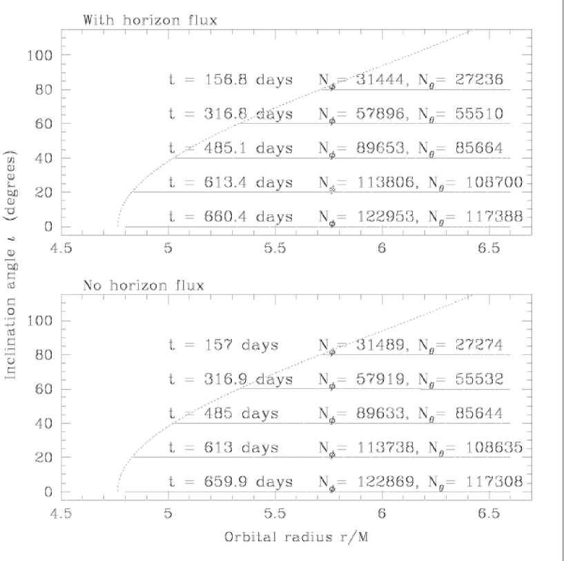
FIG. 5.: Inspiral trajectories in the strong field of a Kerr black hole with $a=0.3594M$. The top panel includes the effects of the down-horizon flux; the bottom panel does not. The span of data is chosen so that the total inspiral duration is similar to that shown in Fig. 2. For this spin, inspiral is nearly identical with the horizon flux included or disincluded: inspiral is slightly faster without horizon flux, but not nearly so much faster as when $a=0.998M$. This is largely because the spin is not fast enough to drag the tidal bulge on the horizon so far forward. In fact, at the innermost orbits the bulge should be essentially in perfect face-on lock with the orbiting body, since $a=0.3594M$ is the spin value at which the horizon spin frequency matches the innermost orbital frequency.

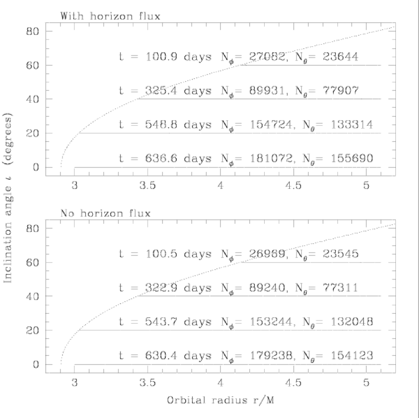
FIG. 6.: Inspiral trajectories in the strong field of a Kerr black hole with $a=0.8M$. The top panel includes the effects of down-horizon flux; the bottom panel does not. The span of data is chosen so that the the total inspiral duration is similar to that shown in Fig. 2. As when $a=0.998M$, inspiral is quicker when the horizon flux is ignored. However, the magnitude of the effect is much smaller. The torque on the orbit that the horizon’s tidal bulge exerts is not as great because the hole rotates less quickly. Also, orbits do not come as close to the horizon for $a=0.8M$ as they do for $a=0.998M$.

FIG. 7.: Inspiral trajectories in the strong field of a Kerr black hole with $a=0.05M$. The top panel includes the effects of down-horizon flux; the bottom panel does not. In this case, inspiral is quicker when the horizon flux is included: the hole’s event horizon acts as an energy sink, as simple intuition suggests it should. This is because the tidal bulge raised on the hole by the orbiting body tends to lag, rather than lead, the orbit. Thus the bulge’s torque on the orbit opposes the orbital motion, causing it to spiral in more quickly.

FIG. 8.: The $+$ polarization of the gravitational waveform for the inspiral trajectory that begins at $\iota=40^{\circ}$ about the $a=0.998M$ black hole, viewed in the hole’s equatorial plane. The upper panel is the waveform at very early times; the lower panel shows the waveform shortly before the inspiraling body plunges into the hole. Notice the very different time scales in the upper and lower panels. This is because of the “chirping” evolution of the frequencies $\Omega_{\phi}$ and $\Omega_{\theta}$ — at late times they are quite a bit larger than they are early on. Many more orbits per unit time are executed late in the inspiral than early.

FIG. 9.: The phase $\Psi_{lmk}$ and amplitude ${\cal H}_{lmk}$ for waveform harmonics $l=2$, $m=2$, and $k$ from 0 to 4, and for spiral into a hole with $a=0.998M$. These amplitudes correspond to measurement in the hole’s equatorial plane. Note that harmonics other than $k=0$ become fairly strong at the end of inspiral. The odd behavior in the amplitude for $k=2-4$ is because of poor computational resolution: the crude parameter space resolution used here was not good enough to accurately capture the change in $Z^{H}_{lmk}$ at high frequencies as the body spirals in.

FIG. 10.: The phase $\Psi_{lmk}$ and amplitude ${\cal H}_{lmk}$ seen in the equatorial plane, for waveform harmonics $l=2$, $m=0$, and $k$ from 0 to 4, and for spiral into a hole with $a=0.998M$. In this case, no frequencies are high enough to cause severe resolution problems, as was the case for $l=2$, $m=2$. Note that the phase evolves from high to low late in the inspiral. This is because the phase is dominated by the behavior of $\Omega_{\theta}$, which chirps backwards when the body gets close to the event horizon; cf. Fig. 11. This is essentially a gravitational redshifting effect. Although this is in principle an interesting signature of the black hole’s strong field, the wave amplitude gets weak as the frequency gets small. This is not surprising, since the rate of change of the binary’s multipole moments decreases with the frequency.

FIG. 11.: Evolution of the orbital frequencies $\Omega_{\phi}$ (solid line) and $\Omega_{\theta}$ (dotted line) for inspiral beginning at $\iota=20^{\circ}$. The upper panel is for inspiral into a black hole with $a=0.998M$, the lower for inspiral into a hole with $a=0.3594M$. In both cases, the behavior of $\Omega_{\phi}$ is qualitatively “normal”: it monotonically chirps upward in a very familiar manner. In the case $a=0.998M$, the behavior of $\Omega_{\theta}$ is comparatively unusual. This is because these orbits are very near to the event horizon — their motion in $\theta$ is slowed as seen by distant observers. When $a=0.3594M$, no orbits come close enough to the horizon for this slowing to have a significant effect. In fact, all orbits in the chosen observation band are at relatively large radius for $a=0.3594M$, which is why all frequencies are quite smaller than when $a=0.998M$ (note the different vertical scales in the two panels).

- [1] K. Danzmann et al., LISA — Laser Interferometer Space Antenna, Pre-Phase A Report, Max-Planck-Institut für Quantenoptik, Report MPQ 233 (1998).
- [2] E. E. Flanagan and S. A. Hughes, Phys. Rev. D 57, 4525 (1998).
- [3] L. S. Finn and K. S. Thorne, Phys. Rev. D 62, 124021 (2000).
- [4] S. Sigurdsson and M. J. Rees, Mon. Not. R. Astron. Soc. 284, 318 (1997).
- [5] S. Sigurdsson, Class. Quantum Grav. 14, 1425 (1997).
- [6] S. A. Hughes, Phys. Rev. D 61, 084004 (2000); 63, 049902(E) (2001).
- [7] S. A. Teukolsky, Ap. J. 185, 635 (1973).
- [8] F. D. Ryan, Phys. Rev. D 56, 1845 (1997).
- [9] J. Levin, Phys. Rev. Lett. 84, 3515 (2000); J. Levin, Phys. Rev. D, submitted; also gr-qc/0010100.
- [10] M. Hartl and E. S. Phinney, in preparation.
- [11] Y. Mino, in preparation [see also talk presented at the 3rd Capra Ranch Meeting, Caltech, June 2000 (online proceedings available at www.tapir.caltech.edu/~capra3)]; A. G. Wiseman, Phys. Rev. D 61, 084014 (2000); A. Ori, Phys. Rev. D 55, 3444 (1997); L. Barack and A. Ori, Phys. Rev. D 61, 061502 (2000); L. M. Burko, Phys. Rev. Lett. 84, 4529 (2000); C. Lousto, Phys. Rev. Lett. 84, 5251 (2000); W. G. Anderson, E. E. Flanagan, and A. C. Ottewill, in preparation; S. Detweiler, Phys. Rev. Lett. 86, 1931 (2001); H. Nakano, Y. Mino, and M. Sasaki, Phys. Rev. D, submitted; also gr-qc/0104012.
- [12] F. D. Ryan, Phys. Rev. D 53, 3064 (1996).
- [13] D. Kennefick and A. Ori, Phys. Rev. D 53, 4319 (1996).
- [14] Y. Mino, unpublished Ph. D. thesis, Kyoto University, 1996.
- [15] K. Glampedakis and D. Kennefick, in preparation.
- [16] S. A. Hughes, Phys. Rev. D 63, 064016 (2001).
- [17] K. S. Thorne, R. H. Price, and D. H. MacDonald, Black Holes: The Membrane Paradigm (Yale University Press, New Haven, CT, 1986).
- [18] S. W. Hawking and J. B. Hartle, Commun. Math. Phys. 25, 283 (1972).
- [19] J. B. Hartle, Phys. Rev. D 8, 1010 (1973); J. B. Hartle, Phys. Rev. D 9, 2749 (1974).
- [20] C. W. Misner, K. S. Thorne, J. A. Wheeler, Gravitation (Freeman, San Francisco, 1973), Chap. 33.
- [21] J. M. Bardeen, W. H. Press, and S. A. Teukolsky, Astrophys. J. 178, 347 (1972).
- [22] W. H. Press, S. A. Teukolsky, W. T. Vetterling, and B. P. Flannery, Numerical Recipes (Cambridge University Press, Cambridge, 1992).
- [23] G. Arfken, Mathematical Methods for Physicists (Academic Press, Orlando, 1985), Chap. 16.
- [24] W. H. Press and S. A. Teukolsky, Astrophys. J. 193, 443 (1974).
- [25] K. S. Thorne, Astrophys. J. 191, 507 (1974).
- [26] R. D. Blandford, private communication.
- [27] R. Moderski, M. Sikora, and J.-P. Lasota, Mon. Not. R. Astron. Soc. 301, 142 (1998).
- [28] Audio representations of these and other gravitational waveforms, in Sun .au format, can be obtained from the URL http://www.tapir.caltech.edu/~hughes/Research/RRKerr/wave_spec.html. Instructions for playing these sounds are given at that URL; please contact the author if you have any technical difficulties.
- [29] F. A. Jenet and T. A. Prince, Phys. Rev. D 62, 122001 (2000).
- [30] In several talks, I have claimed that the amplitude associated with the decreasing frequency will actually be rather large. This was entirely wrong. My statement was based on an earlier stage of this analysis; at the time, the code which interpolates from the parameter space grid to arbitrary parameter space coordinates had a significant bug, which introduced a strong, backward chirping component into the waveform.