Modulating the experimental signature of a stochastic gravitational wave background

Abstract

Detecting a stationary, stochastic gravitational wave signal is complicated by impossibility of observing the detector noise independently of the signal. One consequence is that we require at least two detectors to observe the signal, which will be apparent in the cross-correlation of the detector outputs. A corollary is that there remains a systematic error, associated with the possible presence of correlated instrumental noise, in any observation aimed at estimating or limiting a stochastic gravitational wave signal. Here we describe a method of identifying this systematic error by varying the orientation of one of the detectors, leading to separate and independent modulations of the signal and noise contribution to the cross-correlation. Our method can be applied to measurements of a stochastic gravitational wave background by the ALLEGRO/LIGO Livingston Observatory detector pair. We explore — in the context of this detector pair — how this new measurement technique is insensitive to a cross-correlated detector noise component that can confound a conventional measurement.

I Introduction

While not yet detected, we can be sure that the Earth is bathed in a stochastic gravitational wave background. Contributions to that background arise from the confusion limit of large numbers of distant, conventional gravitational wave sources (e.g., binary systems), early universe physics (e.g., parametric amplification of fluctuations during an inflationary phase), and possibly other “exotic” physics (e.g., cosmic strings) [3]. One of the goals of the ground-based gravitational wave detectors now operating or under construction [4, 5, 6, 7, 8, 9, 10, 11] is to detect or place limits on the amplitude and spectrum of this stochastic gravitational wave background.

A single, isolated gravitational wave detector cannot distinguish between instrumental noise and a weak, stationary cosmic gravitational wave background radiation. At least two detectors are needed, in which case the stochastic signal will be apparent in their cross-correlation. More particularly, the two detectors must i) have an overlapping frequency response, ii) have a separation shorter than the wavelength of their overlapping response, and iii) both sample the same polarization state of the incident radiation. The LIGO Livingston Observatory (LLO) interferometric detector [12, 8] and the Louisiana State University ALLEGRO cryogenic acoustic detector [4, 13, 14], separated by 42.3 km, constitute such a detector pair, capable of providing an experimental bound on the stochastic gravitational wave background at approximately 900 Hz.

Unfortunately, a weak, stationary stochastic signal cannot be distinguished from a similarly weak, stationary noise background that is correlated between the two detectors. Instrumental noise arising from the environment may lead to such a correlated detector noise; consequently, a convincing case must be made that no terrestrial noise source is responsible for any observed correlation. This is a daunting experimental challenge. Any technique that can improve our ability to discriminate between a stochastic gravitational wave signal and a weak correlation of terrestrial origin should be pursued.

Since the signal contribution to the cross-correlation depends on the relative orientation of the detectors (which determines their sensitivity to the two different polarization states), changing the orientation of one of the detectors will modulate the signal contribution to the cross-correlation in a predictable way, allowing us to distinguish the signal from the correlated noise and leading to a significantly improved estimate or bound on the in-band amplitude of a stochastic gravitational wave background. The technique of introducing a controlled signal modulation in order to identify and eliminate systematic environmental effects was conceived by Dicke [15] as the switching radiometer during the development of radar.

The ALLEGRO group has used a planned relocation of their cryogenic detector to a new laboratory in order to implement the capability to re-orient the detector between data-taking periods[16]. This capability now allows for a modulation of the gravitational wave contribution to the detector noise cross-correlation in exactly the manner described. Here we discuss the details of the modulation and how it can be used to improve the reliability of the estimate or limit that we can place on the amplitude of a stochastic gravitational wave background near 900 Hz.

The basic scheme for detecting a stochastic gravitational wave background using two or more gravitational wave detectors was described in [17] and further elucidated in [18, 19, 20]. In Section II we review that work and extend it to the case where the two detectors share a cross-correlated noise component. In Section III we apply these results to the specific case of the ALLEGRO/LLO detector pair, providing the relevant geodetic and physical parameters that are needed to quantify the magnitude of the correlation and describing how to extract the correlation from observations. In Section IV we present results of numerical calculations based on the initial LIGO instrumentation and its proposed upgrade.

II The cross-correlated detector output

A The cross-correlation statistic

The output of each detector — ALLEGRO or LLO — is a single time series, which is the sum of instrumental noise and a projection of the incident gravitational wave strain. Denote the output of LLO as $s_{L}$ and the output of ALLEGRO as $s_{A}$ and define the correlation of $s_{L}$ and $s_{A}$ over an integration time $T_{\text{int}}$ by [17, 18, 19, 20]

$$C(\mathchoice{{\hbox{\boldmath$\displaystyle\Omega_{A}$}}}{{\hbox{\boldmath$\textstyle\Omega_{A}$}}}{{\hbox{\boldmath$\scriptstyle\Omega_{A}$}}}{{\hbox{\boldmath$\scriptscriptstyle\Omega_{A}$}}},\mathchoice{{\hbox{\boldmath$\displaystyle\Omega_{L}$}}}{{\hbox{\boldmath$\textstyle\Omega_{L}$}}}{{\hbox{\boldmath$\scriptstyle\Omega_{L}$}}}{{\hbox{\boldmath$\scriptscriptstyle\Omega_{L}$}}}) := \left<s_{A},S_{L}\right>$$ (2)

$$:= \int_{-T_{\text{int}}/2}^{T_{\text{int}}/2}dt\int_{-T_{\text{int}}/2}^{T_{\text{int}}/2}dt^{\prime}\,s_{A}(t)s_{L}(t^{\prime})Q(t-t^{\prime};\mathchoice{{\hbox{\boldmath$\displaystyle\Omega_{A}$}}}{{\hbox{\boldmath$\textstyle\Omega_{A}$}}}{{\hbox{\boldmath$\scriptstyle\Omega_{A}$}}}{{\hbox{\boldmath$\scriptscriptstyle\Omega_{A}$}}},\mathchoice{{\hbox{\boldmath$\displaystyle\Omega_{L}$}}}{{\hbox{\boldmath$\textstyle\Omega_{L}$}}}{{\hbox{\boldmath$\scriptstyle\Omega_{L}$}}}{{\hbox{\boldmath$\scriptscriptstyle\Omega_{L}$}}}),$$ (3)

where

$$\mathchoice{{\hbox{\boldmath$\displaystyle\Omega$}}}{{\hbox{\boldmath$\textstyle\Omega$}}}{{\hbox{\boldmath$\scriptstyle\Omega$}}}{{\hbox{\boldmath$\scriptscriptstyle\Omega$}}}_{A} :=$$ Angles describing the orientation of ALLEGRO (4)

$$\mathchoice{{\hbox{\boldmath$\displaystyle\Omega$}}}{{\hbox{\boldmath$\textstyle\Omega$}}}{{\hbox{\boldmath$\scriptstyle\Omega$}}}{{\hbox{\boldmath$\scriptscriptstyle\Omega$}}}_{L} := \text{Angles describing the orientation of LLO}.$$ (5)

We discuss the choice of integration kernel $Q\left(\tau;\mathchoice{{\hbox{\boldmath$\displaystyle\Omega$}}}{{\hbox{\boldmath$\textstyle\Omega$}}}{{\hbox{\boldmath$\scriptstyle\Omega$}}}{{\hbox{\boldmath$\scriptscriptstyle\Omega$}}}_{A},\mathchoice{{\hbox{\boldmath$\displaystyle\Omega$}}}{{\hbox{\boldmath$\textstyle\Omega$}}}{{\hbox{\boldmath$\scriptstyle\Omega$}}}{{\hbox{\boldmath$\scriptscriptstyle\Omega$}}}_{L}\right)$ below.

To evaluate the expectation value of $C$ in the presence of signal and noise, write

$$s_{*}:=n_{*}+h_{*},$$ (6)

where $n_{*}$ is the noise and $h_{*}$ is the signal in detector $*$. The signal is, of course, statistically independent of the noise; consequently,

$$\mu := \overline{C}$$ (8)

$$:= \overline{\left<h_{A},h_{L}\right>}+\overline{\left<n_{A},n_{L}\right>},$$ (9)

where the overbar represents an ensemble average. Introducing also the variance of $C$,

$$\sigma^{2}:=\overline{C^{2}}-\overline{C}^{2},$$ (10)

we define the dimensionless signal-to-noise ratio (SNR)

$$\rho:={\mu/\sigma}.$$ (11)

As described above, the integration kernel in equation 3 is at our disposal. If the detector and signal noise spectral densities are known, then $Q$ can be chosen to maximize the signal to noise ratio. Previous work [18, 19, 20] has always assumed that the contribution of the noise cross-correlation (e.g., $\overline{\left<n_{A},n_{L}\right>}$) to the mean $\mu$ vanishes. In Appendix A we consider the more general case where the noise contribution to the ensemble mean cross-correlation is non-zero. In this case the kernel $Q$ that maximizes the SNR can be conveniently expressed in the frequency domain as

$$\widetilde{Q}(f;\mathchoice{{\hbox{\boldmath$\displaystyle\Omega_{A}$}}}{{\hbox{\boldmath$\textstyle\Omega_{A}$}}}{{\hbox{\boldmath$\scriptstyle\Omega_{A}$}}}{{\hbox{\boldmath$\scriptscriptstyle\Omega_{A}$}}},\mathchoice{{\hbox{\boldmath$\displaystyle\Omega_{L}$}}}{{\hbox{\boldmath$\textstyle\Omega_{L}$}}}{{\hbox{\boldmath$\scriptstyle\Omega_{L}$}}}{{\hbox{\boldmath$\scriptscriptstyle\Omega_{L}$}}}):={\gamma(f;\mathchoice{{\hbox{\boldmath$\displaystyle\Omega_{A}$}}}{{\hbox{\boldmath$\textstyle\Omega_{A}$}}}{{\hbox{\boldmath$\scriptstyle\Omega_{A}$}}}{{\hbox{\boldmath$\scriptscriptstyle\Omega_{A}$}}},\mathchoice{{\hbox{\boldmath$\displaystyle\Omega_{L}$}}}{{\hbox{\boldmath$\textstyle\Omega_{L}$}}}{{\hbox{\boldmath$\scriptstyle\Omega_{L}$}}}{{\hbox{\boldmath$\scriptscriptstyle\Omega_{L}$}}})\Omega_{\text{{GW}},0}(f)\over f^{3}\biggl{(}S_{A}(f)S_{L}(f)+S_{AL}(f)^{2}\biggr{)}}~{},$$ (13)

where

$$S_{A} := \left(\text{ALLEGRO noise power spectral density}\right)$$ (14)

$$S_{L} := \left(\text{LLO noise power spectral density}\right)$$ (15)

$$S_{AL} := \left(\text{ALLEGRO/LLO noise cross spectral density}\right)$$ (16)

$$\Omega_{\text{{GW}},0} := \left(\begin{array}[]{l}\text{expected stochastic signal spectrum expressed as a }\\ \text{fraction of the closure density in logarithmic frequency}\end{array}\right)$$ (19)

and $\gamma(f;\mathchoice{{\hbox{\boldmath$\displaystyle\Omega_{A}$}}}{{\hbox{\boldmath$\textstyle\Omega_{A}$}}}{{\hbox{\boldmath$\scriptstyle\Omega_{A}$}}}{{\hbox{\boldmath$\scriptscriptstyle\Omega_{A}$}}},\mathchoice{{\hbox{\boldmath$\displaystyle\Omega_{L}$}}}{{\hbox{\boldmath$\textstyle\Omega_{L}$}}}{{\hbox{\boldmath$\scriptstyle\Omega_{L}$}}}{{\hbox{\boldmath$\scriptscriptstyle\Omega_{L}$}}})$ is the overlap reduction function, which describes the amplitude of the correlation of the gravitational wave signal between the two detectors as a function of their relative orientation [17, 18, 19].

B The overlap reduction function

The overlap reduction function reflects frequency-dependent correlation of the gravitational wave signal in the two detectors and is expressed in terms of their relative orientation and separation. To express $\gamma$ for the ALLEGRO and LLO detectors, focus first on the two arms of the LLO detector, which define a plane (see figure 1). Let $\widehat{\mathchoice{{\hbox{\boldmath$\displaystyle n$}}}{{\hbox{\boldmath$\textstyle n$}}}{{\hbox{\boldmath$\scriptstyle n$}}}{{\hbox{\boldmath$\scriptscriptstyle n$}}}}_{x}$ be the unit vector along the projection onto this plane of the unit vector pointing from the LLO vertex toward the ALLEGRO bar’s midpoint. Taking $\widehat{\mathchoice{{\hbox{\boldmath$\displaystyle n$}}}{{\hbox{\boldmath$\textstyle n$}}}{{\hbox{\boldmath$\scriptstyle n$}}}{{\hbox{\boldmath$\scriptscriptstyle n$}}}}_{z}$ to be orthogonal to the plane and in the direction of increasing altitude, define $\widehat{\mathchoice{{\hbox{\boldmath$\displaystyle n$}}}{{\hbox{\boldmath$\textstyle n$}}}{{\hbox{\boldmath$\scriptstyle n$}}}{{\hbox{\boldmath$\scriptscriptstyle n$}}}}_{y}$ in the plane to form, with $\widehat{\mathchoice{{\hbox{\boldmath$\displaystyle n$}}}{{\hbox{\boldmath$\textstyle n$}}}{{\hbox{\boldmath$\scriptstyle n$}}}{{\hbox{\boldmath$\scriptscriptstyle n$}}}}_{x}$ and $\widehat{\mathchoice{{\hbox{\boldmath$\displaystyle n$}}}{{\hbox{\boldmath$\textstyle n$}}}{{\hbox{\boldmath$\scriptstyle n$}}}{{\hbox{\boldmath$\scriptscriptstyle n$}}}}_{y}$ a right-handed coordinate system.

By construction the arms of the LLO detector also lie in this plane and, by convention, they are referred to as the $X$ and $Y$ arms. Denoting the unit vector in the direction from LLO vertex along the $X$ arm as $\widehat{\mathchoice{{\hbox{\boldmath$\displaystyle X$}}}{{\hbox{\boldmath$\textstyle X$}}}{{\hbox{\boldmath$\scriptstyle X$}}}{{\hbox{\boldmath$\scriptscriptstyle X$}}}}$ and the unit vector in the direction from the vertex along the $Y$ arm as $\widehat{\mathchoice{{\hbox{\boldmath$\displaystyle Y$}}}{{\hbox{\boldmath$\textstyle Y$}}}{{\hbox{\boldmath$\scriptstyle Y$}}}{{\hbox{\boldmath$\scriptscriptstyle Y$}}}}$, $\widehat{\mathchoice{{\hbox{\boldmath$\displaystyle X$}}}{{\hbox{\boldmath$\textstyle X$}}}{{\hbox{\boldmath$\scriptstyle X$}}}{{\hbox{\boldmath$\scriptscriptstyle X$}}}}$ and $\widehat{\mathchoice{{\hbox{\boldmath$\displaystyle Y$}}}{{\hbox{\boldmath$\textstyle Y$}}}{{\hbox{\boldmath$\scriptstyle Y$}}}{{\hbox{\boldmath$\scriptscriptstyle Y$}}}}$ form a right-handed coordinate system with $\widehat{\mathchoice{{\hbox{\boldmath$\displaystyle n$}}}{{\hbox{\boldmath$\textstyle n$}}}{{\hbox{\boldmath$\scriptstyle n$}}}{{\hbox{\boldmath$\scriptscriptstyle n$}}}}_{z}$. It is convenient to introduce the bisector of the pair $(\widehat{\mathchoice{{\hbox{\boldmath$\displaystyle X$}}}{{\hbox{\boldmath$\textstyle X$}}}{{\hbox{\boldmath$\scriptstyle X$}}}{{\hbox{\boldmath$\scriptscriptstyle X$}}}},\widehat{\mathchoice{{\hbox{\boldmath$\displaystyle Y$}}}{{\hbox{\boldmath$\textstyle Y$}}}{{\hbox{\boldmath$\scriptstyle Y$}}}{{\hbox{\boldmath$\scriptscriptstyle Y$}}}})$, in the direction of increasing $\widehat{\mathchoice{{\hbox{\boldmath$\displaystyle X$}}}{{\hbox{\boldmath$\textstyle X$}}}{{\hbox{\boldmath$\scriptstyle X$}}}{{\hbox{\boldmath$\scriptscriptstyle X$}}}}$ and $\widehat{\mathchoice{{\hbox{\boldmath$\displaystyle Y$}}}{{\hbox{\boldmath$\textstyle Y$}}}{{\hbox{\boldmath$\scriptstyle Y$}}}{{\hbox{\boldmath$\scriptscriptstyle Y$}}}}$, and define the angle $\sigma_{L}$ to be the angle between the bisector and $\mathchoice{{\hbox{\boldmath$\displaystyle n$}}}{{\hbox{\boldmath$\textstyle n$}}}{{\hbox{\boldmath$\scriptstyle n$}}}{{\hbox{\boldmath$\scriptscriptstyle n$}}}_{x}$. Then, writing the $TT$-gauge gravitational wave strain as $h_{ij}$, the LLO detector responds to the superposition

$$h_{L}:=h_{ij}d_{L}^{ij}$$ (20)

where

$$\mathchoice{{\hbox{\boldmath$\displaystyle d$}}}{{\hbox{\boldmath$\textstyle d$}}}{{\hbox{\boldmath$\scriptstyle d$}}}{{\hbox{\boldmath$\scriptscriptstyle d$}}}_{L}(\sigma_{L}):={1\over 2}\left[\sin(2\sigma_{L})\left(\hat{\mathchoice{{\hbox{\boldmath$\displaystyle n$}}}{{\hbox{\boldmath$\textstyle n$}}}{{\hbox{\boldmath$\scriptstyle n$}}}{{\hbox{\boldmath$\scriptscriptstyle n$}}}}_{x}\otimes\hat{\mathchoice{{\hbox{\boldmath$\displaystyle n$}}}{{\hbox{\boldmath$\textstyle n$}}}{{\hbox{\boldmath$\scriptstyle n$}}}{{\hbox{\boldmath$\scriptscriptstyle n$}}}}_{x}-\hat{\mathchoice{{\hbox{\boldmath$\displaystyle n$}}}{{\hbox{\boldmath$\textstyle n$}}}{{\hbox{\boldmath$\scriptstyle n$}}}{{\hbox{\boldmath$\scriptscriptstyle n$}}}}_{y}\otimes\hat{\mathchoice{{\hbox{\boldmath$\displaystyle n$}}}{{\hbox{\boldmath$\textstyle n$}}}{{\hbox{\boldmath$\scriptstyle n$}}}{{\hbox{\boldmath$\scriptscriptstyle n$}}}}_{y}\right)-\cos(2\sigma_{L})\left(\hat{\mathchoice{{\hbox{\boldmath$\displaystyle n$}}}{{\hbox{\boldmath$\textstyle n$}}}{{\hbox{\boldmath$\scriptstyle n$}}}{{\hbox{\boldmath$\scriptscriptstyle n$}}}}_{x}\otimes\hat{\mathchoice{{\hbox{\boldmath$\displaystyle n$}}}{{\hbox{\boldmath$\textstyle n$}}}{{\hbox{\boldmath$\scriptstyle n$}}}{{\hbox{\boldmath$\scriptscriptstyle n$}}}}_{y}+\hat{\mathchoice{{\hbox{\boldmath$\displaystyle n$}}}{{\hbox{\boldmath$\textstyle n$}}}{{\hbox{\boldmath$\scriptstyle n$}}}{{\hbox{\boldmath$\scriptscriptstyle n$}}}}_{y}\otimes\hat{\mathchoice{{\hbox{\boldmath$\displaystyle n$}}}{{\hbox{\boldmath$\textstyle n$}}}{{\hbox{\boldmath$\scriptstyle n$}}}{{\hbox{\boldmath$\scriptscriptstyle n$}}}}_{x}\right)\right]$$ (21)

of the incident gravitational waves. In computing the overlap reduction function, $\mathchoice{{\hbox{\boldmath$\displaystyle d$}}}{{\hbox{\boldmath$\textstyle d$}}}{{\hbox{\boldmath$\scriptstyle d$}}}{{\hbox{\boldmath$\scriptscriptstyle d$}}}_{L}$ characterizes the LLO detector.

Assume that symmetry axis of the ALLEGRO bar lies in the $\widehat{\mathchoice{{\hbox{\boldmath$\displaystyle n$}}}{{\hbox{\boldmath$\textstyle n$}}}{{\hbox{\boldmath$\scriptstyle n$}}}{{\hbox{\boldmath$\scriptscriptstyle n$}}}}_{x}\times\widehat{\mathchoice{{\hbox{\boldmath$\displaystyle n$}}}{{\hbox{\boldmath$\textstyle n$}}}{{\hbox{\boldmath$\scriptstyle n$}}}{{\hbox{\boldmath$\scriptscriptstyle n$}}}}_{y}$ plane. and define

$$\sigma_{A}:=\left(\text{the angle between the ALLEGRO symmetry axis and {\hbox{\widehat{\mbox{n}}_{x}}}}\right).$$ (22)

In terms of $\sigma_{A}$ the ALLEGRO detector responds to the superposition

$$h_{A}:=h_{ij}d_{A}^{ij},$$ (23)

where

$$\mathchoice{{\hbox{\boldmath$\displaystyle d$}}}{{\hbox{\boldmath$\textstyle d$}}}{{\hbox{\boldmath$\scriptstyle d$}}}{{\hbox{\boldmath$\scriptscriptstyle d$}}}_{A}(\sigma_{A}) := \left(\hat{\mathchoice{{\hbox{\boldmath$\displaystyle n$}}}{{\hbox{\boldmath$\textstyle n$}}}{{\hbox{\boldmath$\scriptstyle n$}}}{{\hbox{\boldmath$\scriptscriptstyle n$}}}}_{x}\cos\sigma_{A}+\hat{\mathchoice{{\hbox{\boldmath$\displaystyle n$}}}{{\hbox{\boldmath$\textstyle n$}}}{{\hbox{\boldmath$\scriptstyle n$}}}{{\hbox{\boldmath$\scriptscriptstyle n$}}}}_{y}\sin\sigma_{A}\right)$$ (25)

$$\otimes\left(\hat{\mathchoice{{\hbox{\boldmath$\displaystyle n$}}}{{\hbox{\boldmath$\textstyle n$}}}{{\hbox{\boldmath$\scriptstyle n$}}}{{\hbox{\boldmath$\scriptscriptstyle n$}}}}_{x}\cos\sigma_{A}+\hat{\mathchoice{{\hbox{\boldmath$\displaystyle n$}}}{{\hbox{\boldmath$\textstyle n$}}}{{\hbox{\boldmath$\scriptstyle n$}}}{{\hbox{\boldmath$\scriptscriptstyle n$}}}}_{y}\sin\sigma_{A}\right)-{1\over 3}\mathchoice{{\hbox{\boldmath$\displaystyle I$}}}{{\hbox{\boldmath$\textstyle I$}}}{{\hbox{\boldmath$\scriptstyle I$}}}{{\hbox{\boldmath$\scriptscriptstyle I$}}},$$

of the incident gravitational waves. In computing the overlap reduction function, $\mathchoice{{\hbox{\boldmath$\displaystyle d$}}}{{\hbox{\boldmath$\textstyle d$}}}{{\hbox{\boldmath$\scriptstyle d$}}}{{\hbox{\boldmath$\scriptscriptstyle d$}}}_{A}$ characterizes the ALLEGRO detector.

Finally, define the functions $\rho_{k}(\alpha)$ by

$$\left(\begin{array}[]{c}\rho_{1}(\alpha)\\ \rho_{2}(\alpha)\\ \rho_{3}(\alpha)\end{array}\right):={1\over\alpha^{2}}\left(\begin{array}[]{ccc}5\alpha^{2}&-10\alpha&5\\ -10\alpha^{2}&40\alpha&-50\\ 5\alpha^{2}/2&-25\alpha&175/2\end{array}\right)\left(\begin{array}[]{c}j_{0}(\alpha)\\ j_{1}(\alpha)\\ j_{2}(\alpha)\end{array}\right),$$ (26)

where the $j_{k}$ are the spherical Bessel functions of order $k$,

$$\alpha:={2\pi fL/c},$$ (27)

and $L$ is the length of the baseline between the two detectors. The functions $\rho_{k}(\alpha)$ characterize the frequency dependent part of the sensitivity of the detector pair to a stochastic gravitational wave background.

Taking all these pieces together, the overlap reduction can be expressed

$$\gamma(f;\mathchoice{{\hbox{\boldmath$\displaystyle\Omega_{A}$}}}{{\hbox{\boldmath$\textstyle\Omega_{A}$}}}{{\hbox{\boldmath$\scriptstyle\Omega_{A}$}}}{{\hbox{\boldmath$\scriptscriptstyle\Omega_{A}$}}},\mathchoice{{\hbox{\boldmath$\displaystyle\Omega_{L}$}}}{{\hbox{\boldmath$\textstyle\Omega_{L}$}}}{{\hbox{\boldmath$\scriptstyle\Omega_{L}$}}}{{\hbox{\boldmath$\scriptscriptstyle\Omega_{L}$}}}) := \rho_{1}(\alpha)\mathchoice{{\hbox{\boldmath$\displaystyle d$}}}{{\hbox{\boldmath$\textstyle d$}}}{{\hbox{\boldmath$\scriptstyle d$}}}{{\hbox{\boldmath$\scriptscriptstyle d$}}}_{A}:\mathchoice{{\hbox{\boldmath$\displaystyle d$}}}{{\hbox{\boldmath$\textstyle d$}}}{{\hbox{\boldmath$\scriptstyle d$}}}{{\hbox{\boldmath$\scriptscriptstyle d$}}}_{L}+\rho_{2}(\alpha)\left(\mathchoice{{\hbox{\boldmath$\displaystyle\hat{n}$}}}{{\hbox{\boldmath$\textstyle\hat{n}$}}}{{\hbox{\boldmath$\scriptstyle\hat{n}$}}}{{\hbox{\boldmath$\scriptscriptstyle\hat{n}$}}}_{x}\cdot\mathchoice{{\hbox{\boldmath$\displaystyle d$}}}{{\hbox{\boldmath$\textstyle d$}}}{{\hbox{\boldmath$\scriptstyle d$}}}{{\hbox{\boldmath$\scriptscriptstyle d$}}}_{A}\right)\cdot\left(\mathchoice{{\hbox{\boldmath$\displaystyle d$}}}{{\hbox{\boldmath$\textstyle d$}}}{{\hbox{\boldmath$\scriptstyle d$}}}{{\hbox{\boldmath$\scriptscriptstyle d$}}}_{L}\cdot\mathchoice{{\hbox{\boldmath$\displaystyle\hat{n}$}}}{{\hbox{\boldmath$\textstyle\hat{n}$}}}{{\hbox{\boldmath$\scriptstyle\hat{n}$}}}{{\hbox{\boldmath$\scriptscriptstyle\hat{n}$}}}_{x}\right)$$ (29)

$$\qquad{}+\rho_{3}(\alpha)\left(\mathchoice{{\hbox{\boldmath$\displaystyle\hat{n}$}}}{{\hbox{\boldmath$\textstyle\hat{n}$}}}{{\hbox{\boldmath$\scriptstyle\hat{n}$}}}{{\hbox{\boldmath$\scriptscriptstyle\hat{n}$}}}_{x}\cdot\mathchoice{{\hbox{\boldmath$\displaystyle d$}}}{{\hbox{\boldmath$\textstyle d$}}}{{\hbox{\boldmath$\scriptstyle d$}}}{{\hbox{\boldmath$\scriptscriptstyle d$}}}_{A}\cdot\mathchoice{{\hbox{\boldmath$\displaystyle\hat{n}$}}}{{\hbox{\boldmath$\textstyle\hat{n}$}}}{{\hbox{\boldmath$\scriptstyle\hat{n}$}}}{{\hbox{\boldmath$\scriptscriptstyle\hat{n}$}}}_{x}\right)\left(\mathchoice{{\hbox{\boldmath$\displaystyle\hat{n}$}}}{{\hbox{\boldmath$\textstyle\hat{n}$}}}{{\hbox{\boldmath$\scriptstyle\hat{n}$}}}{{\hbox{\boldmath$\scriptscriptstyle\hat{n}$}}}_{x}\cdot\mathchoice{{\hbox{\boldmath$\displaystyle d$}}}{{\hbox{\boldmath$\textstyle d$}}}{{\hbox{\boldmath$\scriptstyle d$}}}{{\hbox{\boldmath$\scriptscriptstyle d$}}}_{L}\cdot\mathchoice{{\hbox{\boldmath$\displaystyle\hat{n}$}}}{{\hbox{\boldmath$\textstyle\hat{n}$}}}{{\hbox{\boldmath$\scriptstyle\hat{n}$}}}{{\hbox{\boldmath$\scriptscriptstyle\hat{n}$}}}_{x}\right),$$

Table I gives the relevant geographic parameters describing LLO detectors [21]; table II does the same for the ALLEGRO detector[16].

III Application: ALLEGRO and LLO

The LLO detector orientation is fixed; however, the orientation of the ALLEGRO detector may be changed by rotating ALLEGRO in its horizontal plane (cf. figure 1). This degree of freedom is described by the angle $\sigma_{A}$, defined in equation 22. As $\sigma_{A}$ varies, $C(\mathchoice{{\hbox{\boldmath$\displaystyle\Omega_{A}$}}}{{\hbox{\boldmath$\textstyle\Omega_{A}$}}}{{\hbox{\boldmath$\scriptstyle\Omega_{A}$}}}{{\hbox{\boldmath$\scriptscriptstyle\Omega_{A}$}}},\mathchoice{{\hbox{\boldmath$\displaystyle\Omega_{L}$}}}{{\hbox{\boldmath$\textstyle\Omega_{L}$}}}{{\hbox{\boldmath$\scriptstyle\Omega_{L}$}}}{{\hbox{\boldmath$\scriptscriptstyle\Omega_{L}$}}})$ will change through the dependence of $\gamma$ on $\sigma_{A}$. To express that variation write the output of detector $k$ as the sum of a gravitational wave signal $h_{k}$ and detector noise $n_{k}$:

$$s_{k}(t):=h_{k}(t)+n_{k}(t).$$ (30)

We can then write the ensemble average of the correlation $C(\mathchoice{{\hbox{\boldmath$\displaystyle\Omega_{A}$}}}{{\hbox{\boldmath$\textstyle\Omega_{A}$}}}{{\hbox{\boldmath$\scriptstyle\Omega_{A}$}}}{{\hbox{\boldmath$\scriptscriptstyle\Omega_{A}$}}},\mathchoice{{\hbox{\boldmath$\displaystyle\Omega_{L}$}}}{{\hbox{\boldmath$\textstyle\Omega_{L}$}}}{{\hbox{\boldmath$\scriptstyle\Omega_{L}$}}}{{\hbox{\boldmath$\scriptscriptstyle\Omega_{L}$}}})$ as a function of $\sigma_{A}$:

$$\overline{C}(\sigma_{A}):=\left(\overline{<h_{A},h_{L}>}+\overline{<n_{A},n_{L}>}\right),$$ (32)

where

$$\overline{\left<h_{A},h_{L}\right>} := T_{\text{int}}\int df\,{3H_{0}^{2}\over 20\pi^{2}}{\gamma^{2}(f;\sigma_{A})\Omega_{\text{{GW}}}(f)\Omega_{0,GW}(f)\over f^{6}\left(S_{A}(f)S_{L}(f)+S_{AL}(f)^{2}\right)},$$ (33)

$$\overline{\left<n_{A},n_{L}\right>} := T_{\text{int}}\int df\,S_{AL}(f;\sigma_{A}){\gamma(f;\sigma_{A})\Omega_{\text{{GW}},0}(f)\over f^{3}\left(S_{A}(f)S_{L}(f)+S_{AL}(f)^{2}\right)},$$ (34)

$$\Omega_{\text{{GW}}} := \left(\begin{array}[]{l}\text{The actual stochastic gravitational wave spectrum}\end{array}\right)$$ (36)

and

$$S_{AL}(f;\sigma_{A}):=\left(\begin{array}[]{l}\text{The ALLEGRO/LLO noise cross-spectral density,}\\ \text{which in general may depend on the orientation angle $\sigma_{A}$}\end{array}\right).$$ (37)

Since $\gamma$ depends on the orientation $\sigma_{A}$ of the ALLEGRO detector, changing ALLEGRO’s orientation changes $\overline{C}$ and allows us to modulate the gravitational wave contribution to $C$ in a predictable way.

Signal correlations between LLO and ALLEGRO occur only in narrow bands centered on the two ALLEGRO bar resonances ($f_{<}$, $f_{>}$; cf. table III). Over the band bounded by the resonances the LLO noise power spectral density $S_{L}$ should be approximately constant and we expect that $\Omega_{\text{GW}}$ will be constant as well. Additionally, for the ALLEGRO/LLO detector pair $\alpha$ (cf. Eq. 27) is small (approximately 0.8) and does not change significantly between the two resonances, so that the overlap reduction function can be treated as frequency independent where the integrands in either of equations 34 and 33 are significant. Further assuming that $S_{AL}$, the ALLEGRO-LLO instrumental noise cross-spectral noise density, is independent of $\sigma_{A}$ and much smaller than either $S_{L}$ or $S_{A}$, we obtain

$$C(\sigma_{A})\simeq T_{\text{int}}\Delta f{\Omega_{\text{{GW}},0}(f_{0})\over f_{0}^{3}S_{A}(f_{0})S_{L}(f_{0})}\left[\gamma^{2}(f_{0};\sigma_{A}){3H_{0}^{2}\over 20\pi^{2}}{\Omega_{\text{GW}}(f_{0})\over f_{0}^{3}}+\gamma(f_{0};\sigma_{A})S_{AL}(f_{0})\right],$$ (39)

where

$$\Delta f := \left({\Delta f_{>}\over S_{A}(f_{>})}+{\Delta f_{<}\over S_{A}(f_{<})}\right)S_{A}$$ (40)

$$S_{A} := {1\over 2}\left[S_{A}(f_{>})+S_{A}(f_{<})\right].$$ (41)

As $\sigma_{A}$ varies the contribution of the stochastic signal to $C$ ($\left<h_{A},h_{L}\right>$, which is quadratic in $\gamma$) varies differently than the contribution of the instrumental noise ($\left<n_{A},n_{L}\right>$, which is linear in $\gamma$). Figure 2 shows, as a solid line, the dependence of $\gamma$ on $\sigma_{A}$. For reference, the dotted line shows the dependence of $\gamma$ on $\sigma_{A}$ at zero frequency. Note how $\gamma$ is approximately sinusoidal in $2\sigma$. Figure 1B shows a schematic of the ALLEGRO bar orientation corresponding to the extrema and null of $\gamma$ as shown in figure 2.

Since the two additive terms in equation 39 depend on $\gamma(f_{0},\sigma_{A})$ differently, varying $\sigma_{A}$ modulates the contribution to $C$ of any correlated noise differently than it modulates the contribution of a real signal. We can use this differential modulation to eliminate the contribution of any correlated noise $S_{AL}$ that is independent of $\sigma_{A}$. Denote the angle $\sigma_{A}$ for which $\gamma$ is maximized as $\sigma_{A,\max}$; similarly, denote the angle $\sigma_{A}$ for which $\gamma$ is minimized as $\sigma_{A,\min}$. Suppose we make an observation of duration $T_{\text{int},\max}$ with ALLEGRO oriented at angle $\sigma_{A,\max}$, and another observation of duration $T_{\text{int},\min}$ at angle $\sigma_{A,\min}$. The expectation value of $C$ for these two observations is

$$\overline{C}(\sigma_{\text{max}})\simeq T_{\text{int},\max}\left(\Delta f{\Omega_{\text{{GW}},0}\over f_{0}^{3}S_{A}S_{L}}\right)\left[\left({3H_{0}^{2}\over 20\pi^{2}f_{0}^{3}}\right){\gamma_{\text{max}}^{2}\Omega_{\text{GW}}}+\gamma_{\text{max}}S_{AL}\right]$$ (43)

and

$$\overline{C}(\sigma_{\text{min}})\simeq T_{\text{int},\min}\left(\Delta f{\Omega_{\text{{GW}},0}\over f_{0}^{3}S_{A}S_{L}}\right)\left[\left({3H_{0}^{2}\over 20\pi^{2}f_{0}^{3}}\right){\gamma_{\text{min}}^{2}\Omega_{\text{GW}}}+\gamma_{\text{min}}S_{AL}\right].$$ (44)

where

$$\gamma_{\max} := \gamma(\sigma_{A,\max})$$ (45)

$$\gamma_{\min} := \gamma(\sigma_{A,\min})$$ (46)

The combination of these two observations

$$C_{0}:={\gamma_{\max}T_{\text{int},\max}{C}(\sigma_{\min})-\gamma_{\min}T_{\text{int},\min}{C}(\sigma_{\max})\over\gamma_{\max}T_{\text{int},\max}+\left|\gamma_{\min}\right|T_{\text{int},\min}}$$ (47)

thus has an expectation value that is independent of the correlated noise $S_{AL}$. In the present circumstance,

$$\gamma_{0}:=\gamma_{\text{max}}\simeq-\gamma_{\text{min}}$$ (48)

If we also make the observations of equal duration,

$$T_{\text{int},\max}=T_{\text{int},\min}=T_{\text{int}}/2$$ (49)

then, following past convention and defining the signal-to-noise ratio $\rho_{0}$ of the observation $C_{0}$ as the ratio of $C_{0}$ to its ensemble variance we have

$$\overline{\rho_{0}}\approx{3H_{0}^{2}\over 10\pi^{2}}\sqrt{T_{\mbox{int}}\Delta f}{\gamma_{0}\Omega_{\text{GW}}(|f_{0}|)\over f_{0}^{3}\sqrt{S_{A}(f_{0})S_{L}(f_{0})+S_{AL}(f_{0})^{2}}}.$$ (50)

IV Numerical Results

Table III describes the theoretical limiting operating characteristics of the current ALLEGRO [4, 13, 14], the initial LIGO Livingston detector [22], and the planned upgrades to ALLEGRO [16] and LIGO [23]. The last two rows give the theoretical limiting sensitivities (90% confidence bounds) for $\Omega_{\text{GW}}(900Hz)$ that are achievable by the detector pairs LIGO I $+$ ALLEGRO and Advanced LIGO $+$ Upgraded ALLEGRO in a one year observation. These limits can be reached only by identifying and accounting for non-gravitational wave inter-detector correlations. Unaccounted correlations of non-gravitational wave origin introduce a systematic error that quickly becomes the limiting factor in an upper limit determination.

Consider, for example, the current generation of ALLEGRO and LLO detectors jointly observing in the presence of a correlated noise

$$\left|S_{AL}(f_{0})\right|=10^{-4}\left(S_{A}S_{L}\right)^{1/2}.$$ (51)

Assume that the stochastic gravitational wave signal amplitude is much smaller: $\Omega_{\text{GW}}$ equal to $10^{-9}$. Suppose first that we are ignore the possibility that the correlated noise component (represented by $S_{AL}$) may be present. Then we would leave the ALLEGRO detector orientation fixed in such a manner as to maximize the overlap with LLO. The dashed lines in figure 3A show, as a function of observing time, the 90% confidence interval (following the construction of [24]) associated with an observed cross-correlation $C$ (cf. eq. 3) equal to the ensemble mean $\bar{C}$. After approximately 0.25 y this most likely observation is clearly no longer consistent with the actual stochastic gravitational wave background amplitude, owing to the systematic error made by excluding the possibility of a correlated noise background. As the observation time increases, the confidence interval on $\Omega_{\text{GW}}$ shrinks, asymptoting on the amplitude of the correlated noise ($S_{AL}$) interpreted as a stochastic gravitational signal.

On the other hand, suppose we admit the possibility of a correlated noise background, of unknown cross-spectral density, changing the orientation of the ALLEGRO detector mid-way through the observation in order that we can construct $C_{0}$ (cf. eq. 47), which is independent of $S_{AL}$. Again referring to figure 3A, the thin gray line shows the 90% confidence interval (following the construction of [24]) on $\Omega_{\text{GW}}$ when the observed $C_{0}$ is equal to its ensemble mean. The confidence interval is, in this case, always consistent with a stochastic gravitational wave background amplitude $\Omega_{\text{GW}}$ of $10^{-9}$. Additionally, in less than 0.45 y this 90% bound limits the signal amplitude to less than the correlated background noise amplitude.

In this example the modulation technique described here provides, in approximately 0.45 y, a bound on the stochastic signal below the correlated noise background amplitude, interpreted as a stochastic gravitational wave signal. Figure 3B shows the integration period required, using this technique, to limit the stochastic background to an amplitude less than the correlated noise background as a function $|S_{AL}(f_{0})|^{1/2}$. The solid line corresponds to the LIGO I/ALLEGRO detector pair while the dashed line, labeled (ii), corresponds to the Advanced LIGO/Upgraded ALLEGRO detector pair. Since, with fixed detectors, the upper limit on the stochastic signal strength is always above the amplitude of the correlated noise, figure 3B shows that, after 1 y of observation with LIGO I + ALLEGRO, an unaccounted for correlation in the background at the level of $\sqrt{S_{AL}(f)}\approx 3\times 10^{-23}~{}1/\sqrt{Hz}$ compromises the measurement. Similarly, after 1 y of observation with Advanced LIGO + Upgraded ALLEGRO, a correlated background with a strain spectral density of $\sqrt{S_{AL}(f)}\approx 2\times 10^{-25}~{}1/\sqrt{Hz}$ will compromise a simple correlation measurement that does not account properly for environmental correlations.

V Discussion

Weber-bar gravitational wave detectors, like ALLEGRO, have placed progressively lower upper limits on the stochastic gravitational wave background amplitude near 900 Hz [25, 26, 27, 28, 29, 30]. The present best upper limit on $\Omega_{\text{GW}}$, set by Astone et al. at 900 Hz [28, 30], used two cryogenic bar detectors operating over a fairly long (600 km) baseline. During a relatively short measurement time they saw no excess correlation between the two bar signals. The planned LIGO-Allegro observations will be made over a much shorter baseline (40 Km); consequently, it correlated environmental noises may be more significant and greater attention will need to be paid to identifying and dismissing them.

In the presence of an undetected correlated background, the best upper limit that can be set will eventually become limited by the bias introduced by the presence of unaccounted correlated detector noise. For the ALLEGRO-LLO pair, correlated noise at a level of $\approx 10^{-4}$ the geometric mean noise spectral density of the two detectors will compromise the observation after less than 1 year of integration time. The possibility that geophysical or other terrestrial correlations could compromise the observation in a single orientation of the detector pair are discussed in[18, 19, 20]; however, those discussions focus on estimating the maximum allowable correlated background for determining a given value for an upper limit. We show here how rotating the ALLEGRO detector allows us to distinguish between a correlated background and a weak, stationary stochastic gravitational wave signal, removing this limit on the sensitivity of a measurement.

The ALLEGRO detector has recently been moved to new quarters and mounted on an air-bearing [16], allowing its orientation with respect to LLO be modulated in manner described here. In a real observation campaign, the frequency with which the detector can be re-oriented is limited from above by the loss of observing time that is introduced through the disturbance of rotating of the detector and the need for the detector to settle down after rotation. Similarly, it is limited from below by the desire to make measurements in multiple orientations. A reasonable compromise would be to re-orient ALLEGRO every $\approx 3-5$ months, while making sure that that exact period is not commensurate with any obvious seasonal or annual cycles.

The degree of improvement possible with this technique will depend on (i) whether the terrestrial background has any component with a characteristic quadrupolar signature that aliases into the stochastic gravitational wave background signature and (ii) the degree to which the background is stationary over the separate periods of measurement in different orientations. Nonetheless, an experiment that modulates the stochastic gravitational wave background signature will improve the quality of any long term observation of $\Omega_{\text{GW}}$.

A The optimal filter in the presence of correlated detector noise

In this appendix we evaluate the kernel $Q$ (cf. eq. 3) that maximizes the signal-to-noise ratio $\rho^{2}$ in equation 11, when a correlated noise component is present.

The general two-detector cross-correlation is given by:

$$C(T):=\int_{-T/2}^{T/2}dt^{\prime}\int_{-T/2}^{T/2}dt^{\prime\prime}s_{1}(t^{\prime})s_{2}(t^{\prime\prime})Q(t^{\prime}-t^{\prime\prime})$$ (A1)

where $s_{i}(t)$ are the signals from the two interferometers and $Q(\tau)$ is the optimal filter kernel to be determined. $s_{i}(t)=h_{i}(t)+n_{i}(t)$, where $h_{i}(t)$ is the signal and $n_{i}(t)$ is the environmental-plus-instrumental noise in each detector.

The correlation can also be expressed in the frequency domain. With the definition of the Fourier transform of a function $r(t)$ given by:

$$\tilde{r}(f):\equiv\int_{-\infty}^{\infty}dt\ e^{-i2\pi ft}\ r(t),$$ (A2)

the correlation measurement is also equal to,

$$C(T):=\int_{-\infty}^{\infty}df\ \int_{-\infty}^{\infty}df^{\prime}\ \delta_{T}(f-f^{\prime})\tilde{s}_{1}^{*}(f)\tilde{s}_{2}(f^{\prime})\tilde{Q}(f^{\prime})\ .$$ (A3)

Here $\tilde{s}_{i}(f)$, and $\tilde{Q}(f)$ are the Fourier transforms of the signals $s_{i}(t)$ and $Q(t-t^{\prime})$. For real $Q(t-t^{\prime})$, the positive and negative frequency values of its Fourier transform are related by $\tilde{Q}(-f)=\tilde{Q}{}^{*}(f)$. The function $\delta_{T}(f-f^{\prime})$ is the finite-time approximation to the Dirac delta function $\delta(f-f^{\prime})$ defined by

$$\delta_{T}(f):=\int_{-T/2}^{T/2}dt\ e^{-i2\pi ft}:={\sin(\pi fT)\over\pi f},$$ (A4)

which arises owing to the windowing property of the finite duration ($T$) measurement.

Generalizing on [20], both the signals and the noise are now assumed to be correlated:

$$\langle\tilde{h}^{*}_{1}(f)\tilde{h}_{2}(f^{\prime})\rangle := \delta(f-f^{\prime}){3H_{0}^{2}\over 20\pi^{2}|f|^{3}}\Omega_{\text{{GW}}}(|f|)\gamma(|f|)$$ (A6)

$$\langle\tilde{n}^{*}_{i}(f)\tilde{n}_{j}(f^{\prime})\rangle := {1\over 2}\delta(f-f^{\prime})S_{ij}(|f|)$$ (A7)

$$\langle\tilde{n}^{*}_{i}(f)\tilde{n}_{j}(f^{\prime})\tilde{n}^{*}_{i}(f^{\prime\prime})\tilde{n}_{j}(f^{\prime\prime\prime})\rangle := {1\over 4}\left(S_{i}(|f|)S_{j}(|f^{\prime}|)\delta(f+f^{\prime\prime})\delta(f^{\prime}+f^{\prime\prime\prime})+\right.$$ (A10)

$$S_{ij}(|f|)S_{ij}(|f^{\prime\prime}|)\delta(f-f^{\prime})\delta(f^{\prime\prime}-f^{\prime\prime\prime})+$$

$$\left.S_{ij}(|f|)S_{ij}(|f^{\prime}|)\delta(f-f^{\prime\prime\prime})\delta(f^{\prime}-f^{\prime\prime})\right)$$

Equation A10 follows from the moment theorem for real Gaussian noise [31, Chapter 3]. $S_{i}(|f|)$ is the power spectral density of the detector noise for the $i^{th}$ detector and $S_{ij}(|f|)$ is the cross-spectral density for the pair $(i,j)$. The factor of $1/2$ in the power spectral densities arises from the definition of the power spectrum as a function for $f>0$.

The cross-correlated signal is a function of relative detector orientation through the overlap reduction factor. Call $C_{+,-}$ the integrated measurement made for two orientations so that the contribution to each from the stochastic gravitational wave background is given by

$$\langle h^{*}_{1}(f)h_{2}(f)\rangle=\pm{3H_{0}^{2}\over 20\pi^{2}|f|^{3}}\Omega_{\text{{GW}}}(|f|)\gamma(|f|)$$ (A11)

For a total measurement interval T, the strategy will be to measure first in one orientation for a fraction of the time, and then to measure in the other orientation for the remainder of the time. Consider the case in which the two intervals are each equal to $T/2$. The two of measurements have the following expectation values:

$$\langle C_{+,-}\rangle:=T/2\int_{-\infty}^{\infty}df\ \left(\pm{3H_{0}^{2}\over 20\pi^{2}}{\Omega_{\rm gw}(|f|)\over|f|^{3}}\gamma(|f|)+S_{12}(f)\right)Q(f).$$ (A12)

The two quantities $C_{+,-}$ can be used to eliminate from the expectation value of the derived signal the effect of the correlated detector noise:

$$\langle C\rangle:=\langle C_{+}-C_{-}\rangle:=T\,\int_{-\infty}^{\infty}df\ \left({3H_{0}^{2}\over 20\pi^{2}}\,{\Omega_{\rm gw}(|f|)\over|f|^{3}}\gamma(|f|)\right)Q(f)\,.$$ (A13)

The optimal filter function follows from maximizing the the signal-to-noise ratio of the cross-correlation:

$${\rm SNR}:={\langle C\rangle\over\sigma_{C}},$$ (A14)

where $\sigma_{C}^{2}=\langle C^{2}\rangle-\langle C\rangle^{2}$ is the variance of the cross-correlation signal $C$. Now the measurements $C_{+,-}$ take place during two distinct intervals each of duration $T/2$. It is reasonable to assume that the fluctuations in these two measurements are not correlated. Then,

$$\sigma_{C}^{2} := \langle C^{2}\rangle-\langle C\rangle^{2}$$ (A16)

$$:= \langle(C_{+}-C_{-})^{2}\rangle-\langle C_{+}-C_{-}\rangle^{2}$$ (A17)

$$:= 2\sigma_{C_{+}}^{2}$$ (A18)

The last simplification follows from the assumed stationarity of the noise and equal measurement intervals with identical statistical properties.

The technique used to evaluate $\sigma_{C_{+}}^{2}$ is similar to that of [20, Eq. 3.61]. First assume that the noise intrinsic to the two detectors is much larger in magnitude than the stochastic gravitational wave background. Then the variance of the measurement will be dominated by the detector noise and not the astrophysical signal. In this case,

$$\sigma_{C_{+}}^{2} := \langle C_{+}^{2}\rangle-\langle C_{+}\rangle^{2}$$ (A20)

$$\approx \int_{-\infty}^{\infty}df\ \int_{-\infty}^{\infty}df^{\prime}\int_{-\infty}^{\infty}dk\ \int_{-\infty}^{\infty}dk^{\prime}\delta_{T\over 2}(f-f^{\prime})\delta_{T\over 2}(k-k^{\prime})$$ (A22)

$$\times\left(\left<\tilde{n}_{1}^{*}(f)\tilde{n}_{2}(f^{\prime})\tilde{n}_{1}^{*}(k)\tilde{n}_{2}(k^{\prime})\right>-\left<\tilde{n}_{1}^{*}(f)\tilde{n}_{2}(f^{\prime})\right>\left<\tilde{n}_{1}^{*}(k)\tilde{n}_{2}(k^{\prime})\right>\right)\tilde{Q}(f^{\prime})\tilde{Q}(k^{\prime})$$

$$\approx \int_{-\infty}^{\infty}df\ \int_{-\infty}^{\infty}df^{\prime}\int_{-\infty}^{\infty}dk\ \int_{-\infty}^{\infty}dk^{\prime}\delta_{T\over 2}(f-f^{\prime})\delta_{T\over 2}(k-k^{\prime})\tilde{Q}(f^{\prime})\tilde{Q}(k^{\prime})$$ (A24)

$$\times~{}{1\over 4}\left[S_{1}(|f|)S_{1}(|f^{\prime}|)\delta(f+k)\delta(f^{\prime}+k^{\prime})+S_{12}(|f|)S_{12}(|f^{\prime}|)\delta(f-k^{\prime})\delta(f^{\prime}-k)\right],$$

where $S_{1}$ and $S_{2}$ are the power spectral densities of the noise in detectors $1$ and $2$, and $S_{12}$ is the cross-spectral density of the noise in the two detectors.

The integrals over $k$, $k^{\prime}$ collapse due to the $\delta$-functions, leaving:

$$\sigma_{C_{+}}^{2} \approx {1\over 4}\int_{-\infty}^{\infty}df\ \int_{-\infty}^{\infty}df^{\prime}\delta_{T\over 2}^{2}(f-f^{\prime})\left(S_{1}(|f|)S_{2}(|f^{\prime}|)+S_{12}(|f|)S_{ij}(|f^{\prime}|)\right)\tilde{Q}(f)\tilde{Q}^{*}(f^{\prime})$$ (A26)

$$\approx {T\over 8}\int_{-\infty}^{\infty}df\ \left(S_{1}(|f|)S_{2}(|f|)+S_{12}(|f|)^{2}\right)|\tilde{Q}(f)|^{2}.$$ (A27)

The last expression is obtained by approximating one of the finite-time delta functions, $\delta_{T\over 2}(f-f^{\prime})$ , as an ordinary Dirac delta function while evaluating the other at $f=f^{\prime}$.

Thus the signal and its variance are given by:

$$\ \langle C\rangle := \langle C_{+}-C_{-}\rangle:=T\int_{-\infty}^{\infty}df\ \left({3H_{0}^{2}\over 20\pi^{2}}|f|^{-3}\ \Omega_{\rm gw}(|f|)\gamma(|f|)\right)Q(f),$$ (A29)

$$\sigma_{C}^{2} \approx {T\over 4}\int_{-\infty}^{\infty}df\ (S_{1}(|f|)S_{1}(|f|)+S_{12}(|f|)^{2})|\tilde{Q}(f)|^{2}.$$ (A30)

Derivation of the optimal function $\tilde{Q}(f)$ proceeds along the same lines as in [20]. The analogous result is:

$$\tilde{Q}(f)\propto{\gamma(|f|)\Omega_{\rm gw}(|f|)\over|f|^{3}\left(S_{1}(|f|)S_{1}(|f|)+S_{12}(|f|)^{2}\right)},$$ (A31)

It can be seen that the effect of correlated inter-detector noise is to replace the product of the single-detector power spectral densities with a sum of this product and the square of the contribution coming from the cross-spectrum. If the cross-spectral density is sufficiently small compared to the single-detector noise spectral densities, then the effect on the optimal filter will be correspondingly small.

TABLE I.: Geographic Data for LIGO Livingston Laboratory (LLO). Positions are with respect to the Earth Centered Frame (ECF): $\hat{z}$ pierces the earth at the north pole, $\hat{x}$ pierces the earth at the intersection of the prime meridian and the equator, and $\hat{y}=\hat{z}\times\hat{x}$

Quantity	Symbol	Value	Units
LLO Vertex	$\{X_{E},Y_{E},Z_{E}\}$	$\{-74276.044,-5496283.721,3224257.018\}$	$m$
	$\{h,\phi,\lambda\}$	$\{-6.568,N30^{\circ}~{}33^{\prime}~{}6.871",W90^{\circ}~{}48^{\prime}~{}50.229"\}$	{m,dms,dms}
$X$ arm
unit vector	$\{\widehat{\mathchoice{{\hbox{\boldmath$\displaystyle X$}}}{{\hbox{\boldmath$\textstyle X$}}}{{\hbox{\boldmath$\scriptstyle X$}}}{{\hbox{\boldmath$\scriptscriptstyle X$}}}}\cdot\widehat{\mathchoice{{\hbox{\boldmath$\displaystyle n$}}}{{\hbox{\boldmath$\textstyle n$}}}{{\hbox{\boldmath$\scriptstyle n$}}}{{\hbox{\boldmath$\scriptscriptstyle n$}}}}_{x},\widehat{\mathchoice{{\hbox{\boldmath$\displaystyle X$}}}{{\hbox{\boldmath$\textstyle X$}}}{{\hbox{\boldmath$\scriptstyle X$}}}{{\hbox{\boldmath$\scriptscriptstyle X$}}}}\cdot\widehat{\mathchoice{{\hbox{\boldmath$\displaystyle n$}}}{{\hbox{\boldmath$\textstyle n$}}}{{\hbox{\boldmath$\scriptstyle n$}}}{{\hbox{\boldmath$\scriptscriptstyle n$}}}}_{y},\widehat{\mathchoice{{\hbox{\boldmath$\displaystyle X$}}}{{\hbox{\boldmath$\textstyle X$}}}{{\hbox{\boldmath$\scriptstyle X$}}}{{\hbox{\boldmath$\scriptscriptstyle X$}}}}\cdot\widehat{\mathchoice{{\hbox{\boldmath$\displaystyle n$}}}{{\hbox{\boldmath$\textstyle n$}}}{{\hbox{\boldmath$\scriptstyle n$}}}{{\hbox{\boldmath$\scriptscriptstyle n$}}}}_{z}\}$	{-0.954574,-0.1415805,-0.2621887}	ECF
$Y$ arm
unit vector	$\{\widehat{\mathchoice{{\hbox{\boldmath$\displaystyle Y$}}}{{\hbox{\boldmath$\textstyle Y$}}}{{\hbox{\boldmath$\scriptstyle Y$}}}{{\hbox{\boldmath$\scriptscriptstyle Y$}}}}\cdot\widehat{\mathchoice{{\hbox{\boldmath$\displaystyle n$}}}{{\hbox{\boldmath$\textstyle n$}}}{{\hbox{\boldmath$\scriptstyle n$}}}{{\hbox{\boldmath$\scriptscriptstyle n$}}}}_{x},\widehat{\mathchoice{{\hbox{\boldmath$\displaystyle Y$}}}{{\hbox{\boldmath$\textstyle Y$}}}{{\hbox{\boldmath$\scriptstyle Y$}}}{{\hbox{\boldmath$\scriptscriptstyle Y$}}}}\cdot\widehat{\mathchoice{{\hbox{\boldmath$\displaystyle n$}}}{{\hbox{\boldmath$\textstyle n$}}}{{\hbox{\boldmath$\scriptstyle n$}}}{{\hbox{\boldmath$\scriptscriptstyle n$}}}}_{y},\widehat{\mathchoice{{\hbox{\boldmath$\displaystyle Y$}}}{{\hbox{\boldmath$\textstyle Y$}}}{{\hbox{\boldmath$\scriptstyle Y$}}}{{\hbox{\boldmath$\scriptscriptstyle Y$}}}}\cdot\widehat{\mathchoice{{\hbox{\boldmath$\displaystyle n$}}}{{\hbox{\boldmath$\textstyle n$}}}{{\hbox{\boldmath$\scriptstyle n$}}}{{\hbox{\boldmath$\scriptscriptstyle n$}}}}_{z}\}$	{0.2977412,-0.4879104,-0.8205447}	ECF
Bearing of			Reference is
ALLEGRO at		$S66.88^{\circ}W$	geodetic
LLO Vertex			north
Angle between
LLO arm			Degrees,
bisector and	$\sigma_{L}$	$39.59^{\circ}$ (Bearing: $S27.28^{\circ}W$)	measured
LLO-			$CCW$ from
ALLEGRO			baseline
baseline

TABLE II.: Geographic Data for ALLEGRO Bar Detector at LSU. For the definition of the Earth Centered Frame see the caption of table I

Quantity	Symbol	Value	Units
ALLEGRO Vertex	$\{X_{E},Y_{E},Z_{E}\}$	$\{-113258.848,5504077.706,3209892.353\}$	$m$
	$\{\phi,\lambda\}$	$\{N30^{\circ}~{}24^{\prime}~{}45.110",W91^{\circ}~{}10^{\prime}~{}43.766"\}$	$\{dms,dms\}$
Bearing of LLO			Reference is
Vertex at		$N66.67^{\circ}E$	geodetic north
ALLEGRO
Angle between		Correlation maximum:$\gamma_{\text{max}}(921Hz)=0.953$	Degrees,
ALLEGRO bar axis		$-5.60^{\circ}$ (Bar axis bearing: $S72.08^{\circ}W$)	measured
and LLO-ALLEGRO	$\sigma_{A}$	Correlation null: $\gamma_{null}(921Hz)=0.0$	$CCW$
baseline for		$40.52^{\circ}$ (Bar axis bearing: $S26.15^{\circ}W$)	from baseline
various values		Correlation minimum:$\gamma_{\text{min}}(921Hz)=-0.893$
of correlations		$84.60^{\circ}$ (Bar axis bearing: $S17.92^{\circ}E$)
LLO - ALLEGRO
baseline distance	$L$	42269.951	m
Angle subtended by
LLO - ALLEGRO	$\beta$	$0.358^{\circ}$	Degrees
baseline at center
of Earth

TABLE III.: Operational characteristics of the LLO and ALLEGRO detectors.

Quantity	Lower ALLEGRO resonant frequency, $f_{<}$	Upper ALLEGRO resonant frequency, $f_{>}$	Units
Frequency	$896.8$	920.3	Hz
ALLEGRO bandwidth, $\Delta f$	$1$	$1$	Hz
Upgraded ALLEGRO bandwidth[16], $\Delta f$	$50$	$50$	Hz
ALLEGRO sensitivity, $h(f)$	$1.8\times 10^{-21}$	$0.85\times 10^{-21}$	$1/\sqrt{Hz}$
LIGO I sensitivity[22], $h(f)$	$1\times 10^{-22}$	$1\times 10^{-22}$	$1/\sqrt{Hz}$
Adv. LIGO narrowband sensitivity[23], $h(f)$	$2\times 10^{-24}$	$2\times 10^{-24}$	$1/\sqrt{Hz}$
$\Omega_{\text{min}}$ for LIGO I + ALLEGRO after 1 year	$1\times 10^{-1}$		at 90% confidence
$\Omega_{\text{min}}$ for adv. LIGO + Upgraded ALLEGRO after 1 year	$2.9\times 10^{-4}$		at 90% confidence

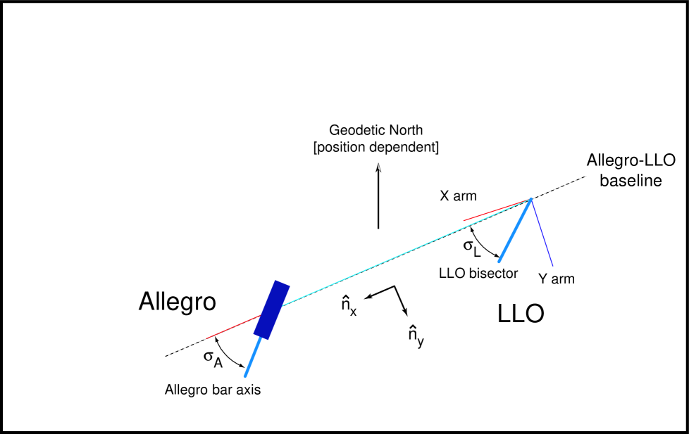
FIG. 1.: A schematic diagram showing how we characterize ALLEGRO and LLO orientations with respect to geodetic north and the LLO-to-ALLEGRO baseline.

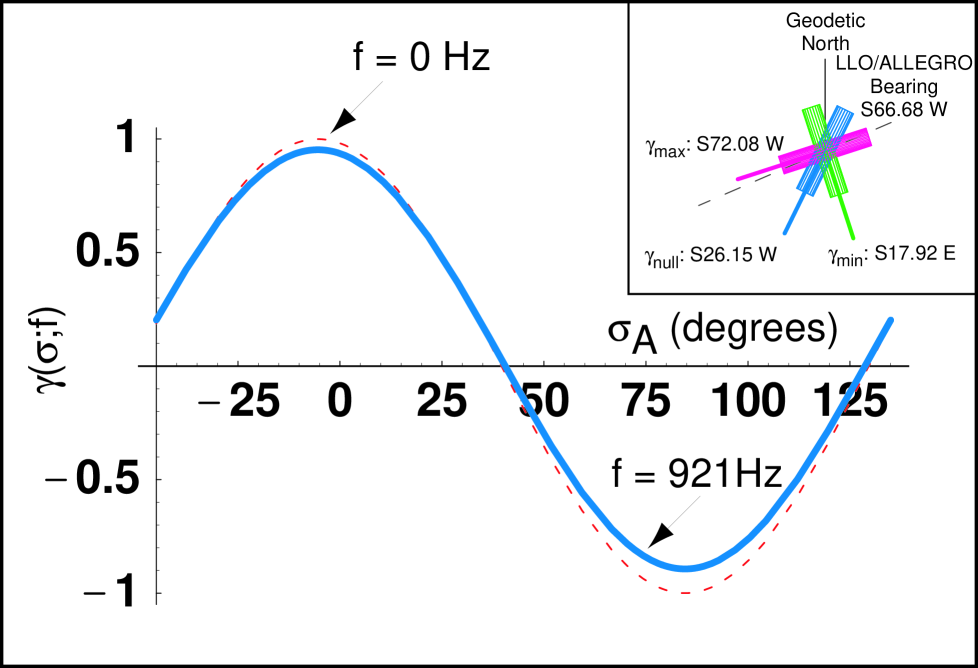
FIG. 2.: The overlap reduction function $\gamma$, which characterizes the dependence of the ALLEGRO-LLO correlation function to an isotropic stochastic signal, depends on the relative orientation of the two detectors. Here we show how this function varies with $\sigma_{A}$, the angle between the ALLEGRO bar axis and the LLO/ALLEGRO baseline (cf. figure 1). The bold, solid line shows the variation of $\gamma$ with $\sigma_{A}$ at the operating frequency of the ALLEGRO detector; for comparison, the dashed line shows the same quantity at DC. Inset B shows the orientation of the ALLEGRO relative to the LLO/ALLEGRO baseline, when $\gamma$ vanishes ($\gamma_{\text{null}}$) and takes on its minimum ($\gamma_{\text{min}}$) and maximum ($\gamma_{\text{max}}$) values.

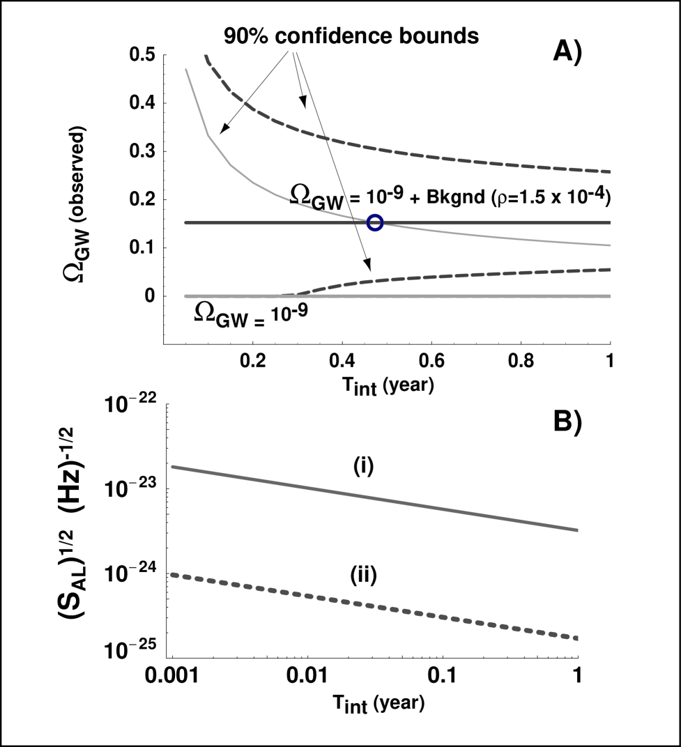
FIG. 3.: A) The dashed lines mark the expected 90% confidence interval, as a function of the observing time, on a stochastic gravitational wave background when a much larger, but unaccounted for, correlated terrestrial noise source is present with a cross spectral density amplitude just $10^{-4}$ the (geometric) mean noise power spectral density in the ALLEGRO and LIGO I detectors. The heavy solid line is the amplitude of the terrestrial noise, (mis)interpreted as a stochastic gravitational wave signal. Note how, after approximately 3 months, the observations are no longer consistent with stochastic gravitational wave amplitude significantly less than the amplitude of the correlated terrestrial noise. The thin line marks the upper limit on the stochastic signal, again as a function of time, when the modulation technique described in this paper is used to make the measurement. The measurement is no longer biased by the terrestrial noise and the upper limit is less than the correlated terrestrial noise amplitude, in this example, in 0.45 y. B) The integration time needed for the upper limit, estimated by the modulation technique described here, to be less than the amplitude of the correlated terrestrial noise amplitude (i.e., to reach the crossing point marked by the bold circle in panel A) as a function of the cross-spectral density. Curve (i) is for LIGO I + ALLEGRO; (ii) is for advanced LIGO + Upgraded ALLEGRO (cf.  table III).