Gravitational Waves from Disks Around Spinning Black Holes: Simulations in Full General Relativity

Abstract

We present fully general-relativistic numerical evolutions of self-gravitating tori around spinning black holes with dimensionless spin $a/M=0.7$ parallel or anti-parallel to the disk angular momentum. The initial disks are unstable to the hydrodynamic Papaloizou-Pringle Instability which causes them to grow persistent orbiting matter clumps. The effect of black hole spin on the growth and saturation of the instability is assessed. We find that the instability behaves similarly to prior simulations with non-spinning black holes, with a shift in frequency due to spin-induced changes in disk orbital period. Copious gravitational waves are generated by these systems, and we analyze their detectability by current and future gravitational wave observatories for large range of masses. We find that systems of $10M_{\odot}$ - relevant for black hole-neutron star mergers - are detectable by Cosmic Explorer out to $\sim 300$ Mpc, while DECIGO (LISA) will be able to detect systems of $1000M_{\odot}$ ($10^{5}M_{\odot}$) - relevant for disks forming in collapsing supermassive stars - out to cosmological redshift of $z\sim 5$ ($z\sim 1$). Computing the accretion rate of these systems we find that these systems may also be promising sources of coincident electromagnetic signals.

I Introduction

To realize the full potential of multimessenger astronomy, it is necessary to model a wide range of gravitational wave (GW) sources. With planned sensitivity upgrades to Advanced LIGO, KAGRA, and Virgo Collaboration et al. (2018) as well as the construction of future more sensitive detectors such as Cosmic Explorer Reitze et al. (2019) and the Einstein Telescope Punturo et al. (2010), a large volume of space will be opened up to GW astronomy in the coming years. Space-based missions such as DECIGO Sato et al. (2017) and LISA Amaro-Seoane et al. (2017) will open up lower frequencies extending down to $0.1\mathrm{Hz}$ and $10^{-4}\mathrm{Hz}$, respectively, which are inaccessible from the ground and will enable the potential detection of entirely new types of sources. With such a large volume of space and such a wide range of frequencies on the verge of being observed, we should be prepared to detect the unexpected, especially once detectors of sufficient sensitivity are brought on-line. It is therefore prudent to investigate sources that have not yet received significant consideration.

While much modeling has been done for compact binary coalescences (for reviews, see Lehner and Pretorius (2014); Shibata and Taniguchi (2011); Faber and Rasio (2012); Paschalidis (2017); Baiotti and Rezzolla (2017); Paschalidis and Stergioulas (2017); Duez and Zlochower (2018); Ciolfi (2020)), comparatively little work has been done exploring the multi-messenger signatures of black holes (BHs) surrounded by massive accretion disks. These systems can arise in various astrophysical environments. For example, disks with rest-masses $\gtrsim 10\%$ of the BH Christodoulou mass can form following black hole-neutron star mergers with rapidly spinning black holes Lovelace et al. (2013) or in the collapse of supermassive stars Shibata and Shapiro (2002); Shapiro and Shibata (2002); Shapiro (2004a); Shibata et al. (2016a); Sun et al. (2017); Uchida et al. (2017a); Sun et al. (2019), and possibly also in collapsars MacFadyen and Woosley (1999a, b); MacFadyen et al. (2001); Heger and Woosley (2002); Heger et al. (2003). Binary neutron star systems with large mass asymmetry can also produce massive disks Rezzolla et al. (2010). Accretion disks onto black holes can be hosts of a wide range of dynamical instabilities that can produce a time-varying quadrupole moment, making them promising GW candidates. In addition, such systems can generate bright electromagnetic signals, and hence they are true multimessenger sources.

A prime example of a dynamical disk instability that develops a time-varying quadrupole moment is the so-called Papaloizou-Pringle Instability (PPI). The PPI is a hydrodynamic instability that grows in fluid tori orbiting in a central potential Papaloizou and Pringle (1984). It results in the growth of non-axisymmetric modes in the rest-mass density $\rho_{0}$ of the form

$$\rho_{0}\propto e^{i(m\phi-\sigma t)},$$ (1)

where $m$ is a positive mode number, and $\sigma$ has a real component that causes pattern rotation and an imaginary component that causes growth. The growth rate is on the order of the orbital timescale of the disk, with $m=1$ being the dominant mode for thick tori Kojima (1986a). For low-$m$ modes in tori of finite extent, exponential growth can be thought of as resulting from the exchange of a conserved quantity between wave-like disturbances on the disk’s inner edge that propagate opposite to the flow, and wave-like disturbances on the disk’s outer edge that propagate with the flow Blaes (1985); Blaes and Glatzel (1986); Goldreich et al. (1986); Narayan et al. (1987); Goodman and Narayan (1988); Christodoulou and Narayan (1992). The existence of unstable PPI modes depends on the profile of a disk’s specific angular momentum, $j$. In a Newtonian context, $j$ is defined as

$$j\equiv rv_{\phi},$$ (2)

where $r$ is the cylindrical coordinate and $v_{\phi}$ is the fluid velocity in the $\phi$-direction. In Papaloizou and Pringle (1985) it was shown that disks are susceptible to the instability when they have a sufficiently shallow $j$ profile:

$$j\propto r^{2-q},\;\sqrt{3}<q\leq 2,$$ (3)

Values of $q$ greater than 2 result in decreasing $j$ profiles, which render disks unstable to an axisymmetric instability discovered previously by Rayleigh Rayleigh (1917).

The PPI has long been known to saturate into persistent non-axisymmetric configurations of orbiting lumps Hawley (1987). Numerical relativity simulations have shown that the PPI can occur in self-gravitating disks around non-spinning BHs Korobkin et al. (2011); Kiuchi et al. (2011), and generate gravitational radiation Kiuchi et al. (2011).

While the conditions under which PPI unstable disks can form dynamically are unclear, in Bonnerot et al. (2015) the simulation of the tidal disruption of a white dwarf by a supermassive BH, found that a nearly axisymmetric torus formed that was unstable to the PPI. This remnant disk had a small mass, and subsequent studies concluded that the resulting GW signal would be weak Nealon et al. (2017); Toscani et al. (2019). The numerical relativity simulations in Lovelace et al. (2013) find that the disks with disk to black hole mass of $\sim 20\%$ forming dynamically following a black hole–neutron star star merger appear to be stable for the times simulated. However, these are limited studies and the parameter space of black hole-neutron stars is large, so that more studies of such mergers are necessary to understand if there exist conditions under which PPI unstable disks form in these systems. On the other hand, the simulations of supermassive stellar collapse in Uchida et al. (2017b) find that the BH disks arising in the process have properties that are favorable for developing the PPI. The above demonstrate that there exist potential channels for the dynamical formation of PPI-unstable disks, and hence it is worth exploring their potential as multimessenger sources with gravitational waves. To better understand how time changing quadrupole moments in disks around black holes result in GW emission, it is more efficient to start with BH-disk initial data and evolve these as a means to study many progenitors at once, instead of performing simulations of the dynamical formation of such disks from different progenitors. This is particularly feasible when the matter is modeled with a $\Gamma$-law equation of state, in which case there is an inherent scale freedom to the set of equations governing the evolution. This is the approach we will adopt in this work.

It is worth noting that magnetized disks unstable to the magneto-rotational instability (MRI) could suppress the PPI growth Bugli et al. (2017). However, both MRI and PPI are exponential instabilities, and both occur on the orbital timescale of the disk. Therefore, if conditions are such that the PPI develops first, then it is plausible that the PPI can grow and survive for longer times. This is supported by the findings of Bugli et al. (2017) who demonstrated that when the $m=1$ mode is initially excited, which is possible in dynamical disk formation scenarios, the PPI dominates the dynamics for several disk orbits before finally succumbing to the MRI. Therefore, it is important to further study the PPI, and most importantly the detectability of the multimessenger signatures of BH-disk systems.

In the context of simulations in full general relativity, self-gravitating disks around black holes were studied in Korobkin et al. (2013) where the runaway instability was investigated. With regards to the focus of this work, the PPI has been explored for self-gravitating disks with constraint-satisfying and equilibrium initial data only around non-spinning black holes Korobkin et al. (2011); Kiuchi et al. (2011). Simulations around spinning black holes, but adopting constraint-violating, and non-equilibrium initial data were performed in Mewes et al. (2016). Here, we initiate a study of the dynamics of the PPI in massive, equilibrium, self-gravitating disks around spinning black holes adopting constraint-satisfying and equilibrium initial data Tsokaros et al. (2019). Our focus is to determine whether the spin of the BH alters the onset of the PPI or its saturation state in any way, and what effect BH spin may have on the detectability of the GW signal, as well as other observables. Our initial disks all obey the same rotation law, have an approximately flat specific angular momentum profile ($q\simeq 2$), and approximately the same mass. In this work we focus on scenarios where the BH spins have dimensionless value of $0$ or $0.7$, either aligned or anti-aligned with the disk orbital angular momentum. In forthcoming work, we will explore the dynamics of misaligned BH spins, where spin-orbit precession effects are expected.

We find that the dynamics of the PPI in our aligned and anti-aligned spin simulations is similar to the non-spinning case, which has been studied previously. However, keeping other quantities nearly fixed, the presence of BH spin causes unavoidable differences in the structure of the disks, which in our case appear as shifts in the orbital frequencies of the disks, thereby affecting the dynamics. The differing innermost stable circular orbit (ISCO) radii also affect the accretion rates, so that the case with the smallest ISCO accretes an order of magnitude more slowly than the others. This result holds in the absence of magnetic fields and for the particular initial inner disk edges we start with; we will explore these effects in future work. Following saturation of the PPI, the GW emission is nearly monochromatic, and is strong enough to be detectable at great distances by Cosmic Explorer, DECIGO, and LISA. In particular, for systems where the disks are $\sim 10\%$ the mass of the central BH, Cosmic Explorer could detect a $10M_{\odot}$ system at 200-320 Mpc, DECIGO could detect a $10^{3}M_{\odot}$ system out to $z\sim 5$, and LISA could detect BH-disk systems with mass ${\rm few}\times 10^{5}M_{\odot}$ out to cosmological redshift of $z\sim 1$. Assuming that 1% of the accretion power escapes as radiation, e.g., powering jets, we find electromagnetic bolometric luminosities of $\mathcal{O}(10^{51-52})$[erg/s] could arise from these systems, making PPI-unstable disks promising multimessenger candidates with GWs for the next generation of GW observatories.

The remainder of this paper is organized as follows: In Section II we describe our initial data, and our methods both for generating the initial data and for the dynamical evolutions. In Section III we discuss the results of the evolutions, comparing the growth and saturation behavior of the instability for all three BH spin states, as well as the GW signals, and the properties of potential electromagnetic radiation. We then scale our results to a number of astrophysically relevant regimes, and analyze the detectability of such systems by LIGO, Cosmic Explorer, DECIGO, and LISA. We conclude in Section IV with a summary of our findings and discussion of future work.

Unless otherwise stated, all quantities are expressed in geometrized units where $G=c=1$. Throughout $M$ designates the Christodoulou mass Christodoulou (1970) of the central BH.

II Methods

Our methods for generating initial data and for performing evolutions have been described in detail elsewhere. Here we briefly summarize these methods, pointing the reader to the appropriate references, and list the properties of our initial data.

II.1 Initial Data

Self-gravitating disks in equilibrium are computed using the COCAL code and the techniques described in Tsokaros et al. (2019). In particular the complete initial value problem is solved for the full spacetime metric including the conformal geometry. The Einstein equations are written in an elliptic form and their solution is obtained through the Komatsu-Eriguchi-Hachisu scheme Komatsu et al. (1989) for black holes Tsokaros and Uryū (2007).

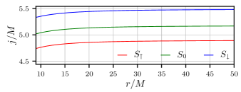
Figure 1: Specific orbital angular momentum ($j$) on the equatorial plane as a function of cylindrical radius on the equatorial plane.

Table 1: Properties of the initial data for the three simulations: $a/M$ is the dimensionless BH spin parameter whose sign implies whether the BH spin is aligned (+) or anti-aligned (-) with the disk orbital angular momentum; $M_{\mathrm{ADM}}$ is the ADM mass of the spacetime; $r_{\mathrm{ISCO}}$ is the cylindrical radius of the vacuum Kerr ISCO with the same BH Christodoulou mass and dimensionless spin; $r_{\mathrm{Inner}},\ r_{c},\ r_{\mathrm{Outer}}$ are the equatorial cylindrical radii of the disk inner edge, maximum density, and outer edge, respectively; $\Omega_{c}$ is the orbital frequency at $r_{c}$; and $M_{\mathrm{disk}}$ is the total disk rest-mass.

Label	$\frac{a}{M}$	$\frac{M_{\mathrm{ADM}}}{M}$	$\frac{r_{\mathrm{ISCO}}}{M}$	$\frac{r_{\mathrm{Inner}}}{M}$	$\frac{r_{c}}{M}$	$\frac{r_{\mathrm{Outer}}}{M}$	$M\Omega_{c}$	$\frac{M_{\mathrm{disk}}}{M}$
$S_{\uparrow}$	0.7	1.13	3.39	9.00	15.6	31.7	$1.61\times 10^{-2}$	0.12
$S_{0}$	0.0	1.14	6.00	9.00	16.9	35.0	$1.47\times 10^{-2}$	0.135
$S_{\downarrow}$	-0.7	1.14	8.14	9.00	18.9	38.9	$1.23\times 10^{-2}$	0.13

Our initial data of self-gravitating disks onto black holes correspond to three BH spin-states, which we will refer to as $S_{0}$ for the non-spinning case, and $S_{\uparrow}$ ($S_{\downarrow}$) for the case with black hole spin aligned (anti-aligned) with the disk orbital angular momentum. Table 1 summarizes the parameters for all cases. Aside from the BH spin, the BH Christodoulou mass ($M$) and the disk inner edge were kept constant, while the rest of the quantities were determined by keeping the disk rest-mass the same to within $\sim 10\%$ from the non-spinning case. Also, the ratio of the disk rest-mass to the BH mass was chosen to be $\sim 0.1$. The initial spacetime closely corresponds to the Kerr metric, with distortions due to the presence of the self-gravitating torus. The disks are modeled as perfect fluids obeying a polytropic equation of state

$$P=k\rho_{0}^{\Gamma},$$ (4)

where $\Gamma=4/3$, appropriate for a radiation-pressure dominated gas. The disk inner edge radius was chosen to be at least 10% greater than the corresponding vacuum Kerr ISCO radius in all cases.

The crucial ingredient for the PPI is the differential rotating law of the disk. As in Tsokaros et al. (2019) we assume that the relativistic specific angular momentum $j=u^{t}u_{\phi}$ profile is given by $j(\Omega)=A^{2}(B_{0}-\Omega)$ with $A=0.1$ and $B_{0}$ a constant that is evaluated during the iteration scheme. This choice leads to a nearly constant ($j\sim r^{0.01}$) angular momentum profile as can be seen in Fig. 1 that renders the disk unstable to the PPI. In terms of the Newtonian Eq. (3) we have $q\approx 2$.

Solutions were then generated satisfying these conditions for each of the three BH spin states and solving the complete initial value problem Tsokaros et al. (2019). The resulting disks differ in their radii of maximum density, which are smaller for more positive spin values. This is responsible for the increase of $M\Omega_{c}$ seen in Table 1, as the values of $\Omega_{c}$ computed for circular geodesics at the corresponding radii in the Kerr metric agree closely with the orbital frequencies of our initial data. The differences in orbital period are small but not insignificant, and end up affecting the dynamics of the disks, as we discuss in Section III.

II.2 Evolution

The BH-disk systems were evolved with the Illinois dynamical spacetime, general relativistic magnetohydrodynamics adaptive-mesh-refinement code Duez et al. (2005); Etienne et al. (2010, 2012). Built within the Cactus/Carpet infrastructure Cac ; Car , this code is the basis of the publicly available counterpart in the Einstein toolkit Etienne et al. (2015). The spacetime metric is evolved by solving the Baumgarte-Shapiro-Shibata-Nakamura (BSSN) equations Shibata and Nakamura (1995); Baumgarte and Shapiro (1998) using the moving-puncture gauge conditions Baker et al. (2006); Campanelli et al. (2006), with the shift vector equation cast into first-order form (see e.g. Hinder et al. (2013)). The fluid is evolved using a $\Gamma$-law equation of state, $P=(\Gamma-1)\rho_{0}\epsilon$, where $\Gamma=4/3$, $\rho_{0}$ is the rest-mass density, and $\epsilon$ the internal specific energy.

II.2.1 Grid hierarchy

The evolution grid hierarchy consists of nested cubes, demarcating 11 concentric refinement levels. Here we will refer to the levels by their index, $n$, where $n=1$ corresponds to the finest level and $n=11$ the coarsest. The finest level half-side length is set to $r_{1}=2.19M$, and the first three are then $r_{n}=2^{(n-1)}r_{1}$ $(n\leq 3)$. The remaining levels have half-side lengths $r_{n}=2^{n}r_{1}$ $(n>3)$. The physical extent of levels $n\geq 4$ is increased by the extra factor of 2 to provide high resolution over the extended area of the disk. Thus, the outermost level has a half-side length of $2250M$.

We set the spatial resolution on the finest level to $dx_{1}=M/25.6$. Each subsequent refinement level has half the resolution of the previous. Therefore, the resolution of refinement level $n$ is given by $dx_{n}=2^{(n-1)}dx_{1}$. We adopt Cartesian coordinates, and equal spatial resolution is chosen for the $x$, $y$, and $z$ directions, without imposing any symmetries on the grid.

II.2.2 Diagnostics

During the evolution, we monitor the normalized Hamiltonian and momentum constraints calculated by Eqs. (40)–(43) of Etienne et al. (2008).

The growth of the unstable density modes was tracked by evaluating the following integral at regular time intervals

$$C_{m}=\int{\sqrt{-g}\mathrm{d}^{3}xu^{0}\rho_{0}e^{im\phi}},$$ (5)

which provides a measure of the non-axisymmetric rest-mass density modes that develop (see e.g. Paschalidis et al. (2015a); East et al. (2016a, b)). Here $g$ is the determinant of the spacetime metric, $u^{0}$ the 0 component of the fluid four-velocity, and $\phi$ the azimuthal angle.

GWs are extracted using the Newman-Penrose Weyl scalar $\psi_{4}$ at various extraction radii. We decompose $\psi_{4}$ into $s=-2$ spin-weighted spherical harmonics up to and including $l=3$ modes. The GW polarizations $h_{+}$ and $h_{\times}$ for each mode are computed by integrating the corresponding mode of $\psi_{4}$ twice with time using the fixed frequency integration technique described in Reisswig and Pollney (2011).

III Results

We performed two types of evolutions of our initial data. First, we simulated the systems in the Cowling approximation (where the spacetime metric is held fixed) to study the early growth of the PPI before it turns non-linear and to corroborate that the characteristics of the instability match those of the PPI. Then we turned on the spacetime evolution and evolved through the instability non-linear growth, saturation and steady state. The results of these simulations are described in the following sections.

III.1 Cowling Approximation

Analytical studies of the PPI looked at its early growth phase for tori in stationary spacetimes, such as in Kojima (1986b) where a Schwarzschild background was assumed. To make contact with these earlier works, we evolved our initial data using the Cowling approximation. While not identical to the disks in Kojima (1986b) (the background spacetime is not precisely Kerr due to the disks’ self-gravity), this allows us to qualitatively compare the early growth in our simulations to analytical expectations, without any of the effects of back-reaction onto the spacetime. More importantly, fixing the background spacetime metric makes the spacetime coordinates well-defined as “Kerr-Schild”-like coordinates. Through the Cowling approximation evolutions the early-time PPI growth rates can be estimated.

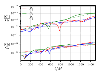
Figure 2: Early amplitude growth of the non-axisymmetric density modes for $m=1$ and $m=2$, evolved with the spacetime background held fixed. A linear fit to each curve is plotted (dotted lines), which indicates the exponential growth rate of the modes.

Table 2: Exponential growth rates of $m=1$ modes in the fixed spacetime evolutions. $\sigma$ is the complex mode frequency, defined in Equation 1. The factor $r_{\mathrm{Inner}}/r_{c}$ was used in Kojima (1986b) to parameterize disk geometries, and is included here to show how our disks relate to those studied in that paper.

Label	$r_{\mathrm{Inner}}/r_{c}$	$\operatorname{Im}(\sigma)/\Omega_{c}$
$S_{\uparrow}$	$5.76\times 10^{-1}$	$1.25\times 10^{-1}$
$S_{0}$	$5.34\times 10^{-1}$	$2.64\times 10^{-1}$
$S_{\downarrow}$	$4.76\times 10^{-1}$	$2.34\times 10^{-1}$

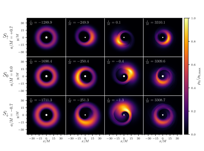
Figure 3: Snapshots of xy-plane cross-sections of the rest-mass density normalized to its maximum value over the entire evolution. Each row corresponds to a single simulation (labeled on the left $S_{\uparrow}$, $S_{0}$, $S_{\downarrow}$), with snapshots arranged chronologically from left to right. The initial time is negative because we have shifted the time such that $t=0$ is the time of the PPI saturation (defined to be the time at which the amplitude of the $m=1$ mode becomes maximum for the first time), which approximately coincides with the third column snapshots. Apparent horizon regions are filled in white, and the snapshots are centered on the BH coordinate centroids. (The change in size of the horizons between the first and second snapshots of each simulation is due to coordinate relaxation.)

Perturbations seeded due to finite-resolution excite all modes to a small degree. At early times the modes grow exponentially until only the fastest-growing ones dominate. For the tori geometries we simulated, analytical studies predict the dominant modes to be $m=1$ and $m=2$ Kojima (1986a). This was observed in our simulations as well. In Figure 2 we plot the $m=1$ and $m=2$ mode amplitudes for all three disks as computed based on Eq. (5). The growth of these modes approximately follows an exponential trend, as shown by the dotted lines in the figure. The estimated exponential growth rates are reported in Table 2, and are of the order $\mathcal{O}(0.1)$ when normalized to $\Omega_{c}$. While a direct comparison with the disks onto Schwarzschild black holes in Kojima (1986b) is not possible, because we have different disks and spacetimes, we find broad agreement with the rates calculated semi-analytically in Kojima (1986b) when comparing models with approximately the same $r_{\mathrm{Inner}}/r_{c}$ - the way Kojima (1986b) parametrized the disks. In addition, we find qualitative agreement with Kojima (1986b) in that the growth rate is exponential, and that the low-$m$ modes dominate, supporting the conclusion that the instability that developes in our simulations is the PPI, as expected from the specific angular momentum profile of the disk.

The self-gravitation of our tori makes the Cowling approximation unsuitable for studying the dynamics through saturation, thus we also evolved them in dynamical spacetime. We turn next to our dynamical spacetime study, which showcases the full dynamics of these systems from early growth until long after saturation.

III.2 Dynamical Spacetime

When the disks are evolved in full general relativity, all three undergo violent non-axisymmetric instabilities. As shown in the first three columns of Figure 3, all three disks develop non-axisymmetric density modes that grow quickly to saturation over a few orbits. Shocks develop during the development of the instability, which redistribute angular momentum until finally the density pattern saturates with the $m=1$ mode dominating the subsequent evolution. The right-most column of the figure contains snapshots of the disks long after saturation, which show that the density mode pattern still persists.

Density mode amplitudes are shown in Figure 4. As in the Cowling approximation evolutions, we find that the fastest modes are still $m=1$ and $m=2$, which are the ones plotted. The figure reveals that the normalized non-axisymmetric $m=1$ and $m=2$ density modes for all three disks saturate near the same values, but the $m=1$ mode dominates. The PPI growth as measured by the $C_{m}$ is still approximately exponential in coordinate time before saturation. In Korobkin et al. (2011) the PPI growth rate was reported to be slightly greater in a dynamical spacetime than for a fixed spacetime. Although statements based on coordinate time are gauge-dependent in evolutions where the spacetime and coordinates are dynamical, our results show qualitative agreement with this previous finding: the instabilities grow more quickly in the dynamical spacetime evolutions.

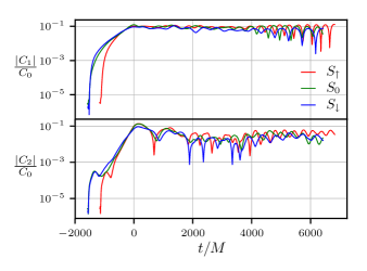
Figure 4: Full dynamical evolution of the amplitude of the non-axisymmetric $m=1$ and $m=2$ density modes, normalized by the $m=0$ mode amplitude.

In Figure 5 we compare the spectra of the modes, which are similar across the different cases, with the only significant difference being the location of the peak frequency. We find that the peak frequencies correlate closely with the orbital frequencies at maximum density of the initial data. When plotted relative to each disk’s respective orbital frequency, as in Figure 6, the spectra are nearly identical. The spectra for the $m=2$ modes are less clean, but their peak frequencies are double that of the $m=1$ modes in each case, as anticipated when the dynamics is driven by an $m=1$ mode East et al. (2016a), and therefore they are nearly equal for the different cases when scaled by orbital frequency. We also find that higher-$m$ modes are excited but are orders of magnitude weaker than the $m=1$ and $m=2$ modes.

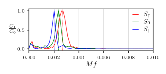
Figure 5: Normalized spectra of the $m=1$ non-axisymmetric density mode for the three disks. The dominant frequency of the $m=2$ modes is twice that of $m=1$ in each case.

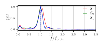
Figure 6: Spectra of the m=1 mode from Figure 5, plotted relative to each disk’s respective initial orbital frequency at maximum density. The plot shows reveals that the density modes among different cases are in close agreement agreement.

The above results suggest that in the case of aligned or anti-aligned BH spins, we do not observe any significant difference from the PPI’s established behavior around non-spinning black holes. The only change is a frequency shift that matches the orbital frequency shift between the initial data for each case. As discussed in Sec. II.1, these orbital frequency shifts originate from slight differences in the initial data and are driven by the BH spin. If we were to alter the disk parameters so that the initial orbital frequencies match, we would have to choose disks with different values for $r_{\mathrm{inner}}$ or $M_{\mathrm{disk}}$ or change the rotation law, which could alter the PPI in other ways. Here we chose to fix $R_{\mathrm{inner}}$ and approximately $M_{\mathrm{disk}}$ instead, to focus on the effects of the BH spin.

Ultimately, the effect of BH spin is both indirect and unavoidable. Although there seems to be no direct change in the nature of the PPI due to spin (at least not for spins up to $a/M=0.7$), the different spin states still force disks to assume different structures, which alter the PPI in a predictable way. Therefore, spin is an important parameter to consider when exploring the range of dynamics of possible PPI-unstable BH-disk systems, and predicting their gravitational-wave signatures.

As mentioned above, while the disk density modes are useful for understanding the character of the instability, they suffer from gauge ambiguities. We can lift these ambiguities by studying the instability through the gravitational radiation instead, which can be extracted unambiguously.

III.3 Gravitational Wave Signal

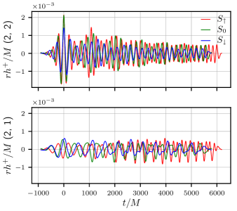
Figure 7: Strain waveforms for the $l=2$, $m=2$ (top), and $m=1$ (bottom) radiation multipoles. To ease comparison, phases have been rotated to align at maximum amplitude of the $l=2$, $m=2$ mode.

In Fig. 7 we compare the $l=2$, $m=2$ and $l=2$, $m=1$ multipole moments of the gravitational radiation. All three cases exhibit an initial burst corresponding to the saturation of the instability, and then a relaxation to a quasi-monochromatic signal of lower amplitude. The $l=2$, $m=2$ plot in Fig. 7 exhibits a noticeable difference between the peak amplitudes of the signal from disks $S_{\uparrow}$ and $S_{0}$, and disk $S_{\downarrow}$. What is the reason for the difference in signal amplitude? The quadrupole formula provides insight. To a rough approximation we can model the BH-$m=1$ mode-dominated disk system as a pair of orbiting point masses, one representing the black hole, and one representing the displaced center-of-mass of the dominant non-axisymmetric mode. In this model, we assume that the effective reduced mass $\mu$ is essentially the disk mass due to the small mass ratio. Then, assuming that the orbital separation $r_{c}$ and reduced mass $\mu$ change slowly relative to $\Omega_{c}$, the quadrupole formula predicts the strain signal for viewpoints in the orbital plane to be (for derivation, see Lai et al. (1994); see also Paschalidis et al. (2009)):

$$rh=4r_{c}^{2}\mu\Omega_{c}^{2}e^{2i\Omega_{c}t},$$ (6)

where $\Omega_{c}$ is the orbital frequency, which we also take from Table 1. All three disks have nearly identical profiles of $|C_{m}|/C_{0}$ for $m=1$ and $m=2$, with the higher-$m$ having much smaller amplitudes, and after $\sim 2500M$ accretion has resulted in similar disk masses. Therefore, in the model we can assume they each have the same values of $\mu$ (the orbital motion of the effective point mass can account for the phase rotation of $C_{m}$, since they are observed to have frequencies proportional to $m$). Then we can use the values of $\Omega_{c}$ and $r_{c}$ from Table 1 to compute the expected amplitude ratios between the three disks. We find that the amplitude of $S_{0}$ should be $1.14\times$ that of $S_{\downarrow}$, and the amplitude of $S_{\uparrow}$ should be $1.21\times$ that of $S_{\downarrow}$, which is in broad agreement with what we observe. Hence, the difference in GW amplitude can be accounted for as yet another effect of the shift in disk orbital frequency due to the different BH spin states.

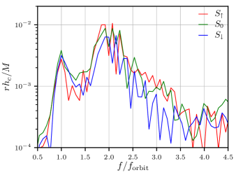
Figure 8: Frequency-domain comparisons of the polarization-averaged characteristic strain (defined in (7,8)) of the GWs from the three disks, with respect to the orbital frequency. All radiation multipoles are combined with appropriate spin-weight spherical harmonics, assuming a viewing angle of $\theta=\pi/2.34$ away from the orbital axis, which results in the observed amplitude of the $l=2,m=2$ mode being equal to its direction-averaged value.

To quantify the frequency-domain behavior we calculate the characteristic strain (see Moore et al. (2014)), which is defined only over positive frequencies as,

$$h_{c}=2f|\tilde{h}^{\mathrm{res}}|,$$ (7)

where $\tilde{h}^{\mathrm{res}}$ is conventionally taken to be the Fourier transform of the interferometer response to the incoming strain waveform $h$. However, in this work we will consider multiple detectors with different response functions, so we instead choose,

$$\tilde{h}^{\mathrm{res}}=\sqrt{\frac{|\tilde{h}_{+}|^{2}+|\tilde{h}_{\times}|^{2}}{2}},$$ (8)

where $\tilde{h}_{+},\tilde{h}_{\times}$ are the Fourier transform of the $+$ and $\times$ polarizations of the incoming signal. For the remainder of this paper we will take $h_{c}$ to be the “polarization-averaged” characteristic strain, defined through Eqs. (7) and (8).

Figure 8 compares the characteristic strain of each waveform for an angle between the line of sight and the orbital plane that corresponds to a value such that ${}_{-2}Y^{2}_{2}$ equals its angle-averaged value. All extracted radiation multipoles up to and including $l=3$ are used in the calculation. Once again, measured relative to the orbital frequencies the spectral peaks of the 3 different cases align well with each other, with the dominant peaks occurring at $f_{\mathrm{orbit}}$ and $2f_{\mathrm{orbit}}$ for the $m=1$ and $m=2$ modes, respectively. This figure demonstrates in a gauge-independent way the results we found using the density modes in the previous section: the dominant non-axisymmetric modes are the $m=1$ and $m=2$.

III.4 Accretion and possible electromagnetic counterparts

In addition to GWs, BH-disk systems are likely to emit electromagnetic (EM) radiation because of accretion. As the disk undergoes dynamical relaxation, shocks within the disk redistribute angular momentum, which allows accretion to proceed. Associated with this accretion mechanism bright, electromagnetic counterparts are possible. While there is no source of (effective) viscosity in our simulations, if net poloidal magnetic flux is accreted onto the black hole at the rate found in our simulations it would power jets Paschalidis et al. (2015b). In cases where a viscous dissipation mechanism is involved emission is expected to arise locally as gravitational binding energy is released when matter is gradually transported to circular orbits closer to the BH. If the disks become dense and hot enough they can also generate copious neutrino emission, but this is more relevant to stellar mass systems. The power available for EM emission is usually taken to be proportional to the accretion power. Under this assumption we can therefore expect the luminosity of the disk to obey

$$L_{\mathrm{EM}}=\epsilon\dot{M}_{\mathrm{disk}}c^{2},$$ (9)

where $\dot{M}_{\mathrm{disk}}$ is the rest-mass accretion rate, and $\epsilon$ is the efficiency for converting accretion power to EM luminosity. For geometrically thin disks in the Kerr metric the difference in binding energy between infinity and ISCO allows maximum possible values of $\epsilon$ up to 40%, depending on BH spin, and in astrophysically realistic settings $\epsilon$ is typically estimated to be $\approx$10% Shapiro and Teukolsky (1983). For thick disks around BHs arising from magnetized black hole-neutron star mergers, binary neutron star mergers or supermassive stellar collapse Poynting dominated jet power satisfies $\epsilon\simeq 0.1$%-$0.5$% Paschalidis et al. (2015b); Ruiz et al. (2016); Sun et al. (2017); Ruiz et al. (2019). Here we will adopt a nominal value of $\epsilon=1$%, but it is important to keep in mind that it is possible that $\epsilon\ll 1\%$. We will test this assumption in a forthcoming work where we treat the effects of magnetic fields. Note that even if magnetic fields allow the PPI to operate for a few orbits Bugli et al. (2017), the GW signal would likely be accompanied by a magnetically powered jet.

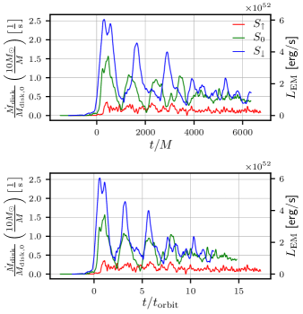
Figure 9: Rest-mass accretion timescales and estimated EM luminosities for the cases in our study. The accretion timescales (inverse accretion rates) are marked on the left y-axis, and scale with $1/M$ as indicated by the axis label. The right y-axis shows the estimated bolometric luminosities (which do not scale with mass) using Eq. (9) with $\epsilon=1\%$. The bolometric luminosities of $S_{0}$ and $S_{\downarrow}$ are $\mathcal{O}(10^{52})$[erg/s], while $S_{\uparrow}$ only achieves $\mathcal{O}(10^{51})$[erg/s]. In the top panel the coordinate time is normalized to the BH mass. In the bottom panel the time is scaled by the initial orbital period at maximum density, showing that the period of the accretion spikes scales with the orbital period for the three simulations.

In Figure 9 the rest-mass accretion rate is plotted for all three cases. Disks $S_{0}$ and $S_{\downarrow}$ display repeated spikes in their accretion rates, the periods of which scale approximately with $t_{\mathrm{orb}}$, as shown in panel (b). As time goes on the accretion rates of $S_{0}$ and $S_{\downarrow}$ become less volatile, so the spiking is likely a transient effect associated with the relaxation of the initial data into the PPI saturation phase. The root cause of this spiking is unclear, and it is unknown whether these features are generic to PPI-unstable disks or unique to the specific initial configurations we evolved.

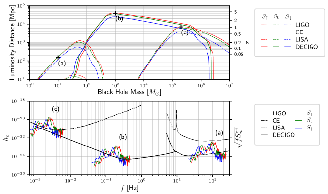
Figure 10: Top: Maximum detection distances for systems over a range of BH masses, assuming a detection threshold of SNR=8 (sky & polarization averaged). The colors and line patterns correspond to the spin state and detector, as shown in the legend. Three hypothetical sources are marked by crosses, representing the most distant systems at three different BH masses that can be detected assuming the $S_{\uparrow}$ waveform: (a) $10M_{\odot}$, $150$ Mpc; (b) $1000M_{\odot}$, 40000 Mpc ($z=4.3$); (c) $2\times 10^{5}M_{\odot}$, $7000$ Mpc ($z=1.02$). Bottom: Characteristic strain curves (see equations (7) and (8))) for each spin state (colored lines) with overlaid the sky-averaged detector characteristic sensitivity curves for LIGO (dotted), Cosmic Explorer (dot-dashed), DECIGO (solid), and LISA (dashed). The labels by each set of characteristic strain curves indicate the BH mass and luminosity distance of the source, which are marked on the bottom panel. The area between the sensitivity and signal curves determines the SNR. In both plots, we consider only the part of the signal after $t=1000M$, as the earlier portion may be strongly influenced by transients arising from hydrodynamic relaxation of the initial data.

After the accretion rates settle down, the disk in case $S_{\uparrow}$ ends up with a significantly suppressed rate relative to $S_{0}$ and $S_{\downarrow}$. A likely reason for this is that the ISCO is further away from the inner edge of the disk in $S_{\uparrow}$ than it is for $S_{0}$ and $S_{\downarrow}$ (for the latter the ISCO nearly coincides with the inner edge). This difference in accretion rate also translates to significant difference in estimated bolometric luminosity. As shown by the right axis of Fig. 9, after the transient accretion spikes die away, the luminosities of $S_{0}$ and $S_{\downarrow}$ are $\mathcal{O}(10^{52})$[erg/s], while $S_{\uparrow}$ is an order of magnitude dimmer at $\mathcal{O}(10^{51})$[erg/s]. Even the dimmest of these bolometric luminosities is high enough to be detectable over a large distance, and makes such disks potentially promising sources of electromagnetic radiation, provided the conversion efficiency to observable frequencies is not too low. Note that for stellar mass black holes it is possible that much of that power is in the form of neutrinos instead, but we would still expect jets to arise if net poloidal magnetic flux is accreted onto the black ho.e

The accretion rate is also important as the determiner of the disk lifetime, and hence the time over which the system emits gravitational radiation. Notably, the $S_{\uparrow}$ accretion timescale is significantly greater than that reported by Kiuchi et al. (2011) for the strictly non-spinning case. Scaling the rates reported by Kiuchi et al. (2011) to a 10 $M_{\odot}$ BH surrounded by a disk of $\sim$%10 its mass, we obtain an accretion timescale between $\sim 0.5$s and $\sim 4$s. This is consistent with the $S_{0}$ timescale we find, which is about 2.5s. However, for $S_{\uparrow}$, the accretion timescale is about 10s (as can be seen in Figure 9), which is significantly longer. This improves the detection prospects of such BH-disk systems, which are analyzed in the next section. However, we note that magnetic fields should be accounted for to test if these accretion rates are robust against the MRI. This will be the topic of future work of ours.

III.5 Detectability of gravitational waves

In the previous sections, all results were reported in terms of dimensionless quantities natural for the system being considered. To assess detectability it is necessary to give the systems a definite physical scale. Both GR and the equations governing the $\Gamma$-law perfect fluid scale with the system’s total gravitational mass. Since in our simulations we consider disks roughly $10\%$ the mass of the central BH, it is the BH mass that primarily determines the mass of the system. In this section we exploit the scale-invariance of our simulations to apply our results to a broad range of masses and astrophysical systems.

There are three mass ranges of astrophysical relevance. On the more massive side are BH-disk systems of $10^{3}$-$10^{6}M_{\odot}$. It has been shown that systems of such masses, with disks $\approx 10$% $M$, can be formed by collapsing super-massive stars (SMS) Shibata and Shapiro (2002); Shapiro and Shibata (2002); Shapiro (2004a); Sun et al. (2017); Uchida et al. (2017a). Such SMS collapses have been conjectured to occur in the early Universe, providing seed BHs which may grow into supermassive BHs Loeb and Rasio (1994); Shapiro (2003); Koushiappas et al. (2004); Shapiro (2004b, 2005); Begelman et al. (2006); Lodato and Natarajan (2006); Begelman (2009), the early appearance of which at $z\sim 7$ is challenging to explain (see reviews Haiman (2012); Latif and Ferrara (2016); Smith et al. (2017)). Masses between several tens to a few hundred $M_{\odot}$ could be populated by the remnants of metal-free Population III stars, which are expected in this mass range and are believed to have their peak formation rates between $z\sim 5-8$ Tornatore et al. (2007); Johnson et al. (2012). Observations have revealed Pop III stars at $z\sim 6.5$ Sobral et al. (2015), providing support for this picture. For masses $25$-$140M_{\odot}$ and greater than $260M_{\odot}$ Pop III stars are expected to end their lives as collapsars Heger and Woosley (2002); Heger et al. (2003), producing failed supernova and BH-disk remnants suspected of powering distant, long gamma-ray bursts MacFadyen and Woosley (1999b); MacFadyen et al. (2001). The least massive potential progenitors are binary neutron star (NSNS) and neutron star-BH (BHNS) mergers, the final BH masses of which are expected to cover the approximate range $3$-$20M_{\odot}$ Voss and Tauris (2003). We point out that while an EOS with $\Gamma=4/3$ is likely appropriate for supermassive and Pop III stars Shapiro (2004a); Shibata et al. (2016b, a), it is not appropriate for NSNS and BHNS systems where nuclear matter is at play. Thus, when applying our results to low-mass systems they should only be viewed as approximate.

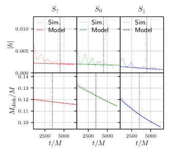
Figure 11: Top row: Signal amplitude time evolution (faint solid lines) and model amplitude time evolution (dashed lines). Bottom row: Total disk mass (faint solid lines) and modeled disk mass (dashed lines). The model was fit to the data only in the regions to the right of the vertical dotted lines, to avoid interference by transient features in the GW signal and accretion rate.

After scaling to the appropriate mass scale, the signals are propagated from the source frame to the observer frame through a flat $\Lambda$CDM cosmology, and the characteristic strain is computed (see equations (7) and (8)). In our analysis we remove the first $\Delta t=1000M$ of the signal to eliminate the initial violent hydrodynamic relaxation of the initial data as the instability develops. As in Fig. 8 we adopt an angle $\theta=\pi/2.34$ for the orbital inclination, which results in the dominant $l=2,m=2$ mode amplitude being equal to its $\theta$-averaged value. We then compute a “sky-averaged” signal-to-noise (SNR) for such an event if observed by Advanced LIGO Collaboration et al. (2018), Cosmic Explorer Reitze et al. (2019), DECIGO Sato et al. (2017), or LISA Amaro-Seoane et al. (2017), assuming an optimal matched filter. Sensitivity curves for the three ground-based observatories were obtained from Gro , divided by the sky-averaged antenna response function for a $90^{\circ}$ interferometer (see equation 51 of Moore et al. (2014)). The analytic approximations given in Yagi and Seto (2011) and Robson et al. (2019) were used for the DECIGO and LISA sky-averaged sensitivities, respectively.

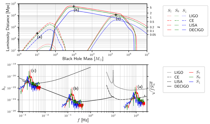
Figure 12: Same as Fig. 10 but for the extrapolated signal. The three hypothetical sources representing the most distant systems detectable for the same three BH masses from Figure 10 now become: (a) $10M_{\odot}$, $300$ Mpc; (b) $1000M_{\odot}$, 60000 Mpc ($z=6.08$); (c) $2\times 10^{5}M_{\odot}$, $11000$ Mpc ($z=1.47$).

The results of the SNR calculation using the simulated part of the GW signal (after $1000M$) for each case are shown in Figure 10. The top panel shows the maximum distance or redshift a system of given mass would be detectable assuming an SNR detection threshold of 8. From the plot it becomes clear that Advanced LIGO can detect such systems at a maximum distance of just under $\sim 20$ Mpc (for the case of a $20M_{\odot}$ BH). On the other hand, Cosmic Explorer will be able to detect a $20M_{\odot}$ source out to $\sim 400$ Mpc, and can detect a 10 $M_{\odot}$ system (marked by a $+$ and labeled (a)) out to 150 Mpc. It is therefore possible that future ground-based detectors could observe such systems.

Space-based observatories will be able to detect more distant and massive sources. As shown in Figure 10, DECIGO and LISA are well suited to detect systems with masses $10^{3}$-$10^{6}M_{\odot}$, and can detect them out to many Gpc. DECIGO in particular, owing to its superb sensitivity, would be able to detect such systems out to several tens of Gpc. A system with mass $10^{3}M_{\odot}$ (labeled as source (b)) can be detected much further out than any other system mass, with the maximum distance corresponding to a cosmological redshift of $z=4.3$. On the other hand, LISA will be able to detect BH-disk systems with mass $10^{5}-10^{6}M_{\odot}$ out to cosmological redshift of $z=1$ (for the source mass labeled (c)). The characteristic strain for sources with masses corresponding to those labeled (a), (b), (c) in the top panel are shown in the bottom panel for each of the three spin states we simulated. We also plot the corresponding sensitivity curves of LIGO, Cosmic Explorer (labeled CE in the figure), DECIGO and LISA.

In Figure 10, we considered just the GW signal that was extracted from in our simulations (excluding the first $1000M$). However, at the end of our simulations the disks still emit significant gravitational radiation, and the orbiting $m=1$ over-densities responsible for that radiation appear to be stable features in all three cases. Consequently, we expect that the disks will continue emitting a strong GW signal until a significant amount of the rest-mass has been accreted, increasing the total signal duration.

To obtain a better estimate of the detectability of BH-disk systems, we therefore need to extrapolate beyond the portion of the signal that was simulated. For simplicity, we restrict ourselves to modeling the dominant $l=2$, $m=2$ mode. Motivated by Equation 6, we assume that the signal will be similar to that of two orbiting point masses. Due to accretion, mass is slowly transferred from the disk to the BH. The simulation data show that the disk rest-mass decays approximately exponentially. This can be modeled in the quadrupole formula by inserting $\mu\propto e^{-\gamma t}$ into Eq. 6. As long as $\gamma$ is small relative to the orbital frequency $\Omega_{c}$, and we can ignore the time derivatives due to mass transfer when taking time derivatives of the quadrupole moment. Under these assumptions, the signal after the transient period will be of the form

$$h=Be^{(i\omega_{0}-\gamma)t}.$$ (10)

This form indeed matches the observed late-time behavior of our simulated GW signal. To match this model to the observed waveforms we first chose the value of $\omega_{0}$ via a least-squares linear fit to the unrolled phase of the complex $l=2$, $m=2$ strain. Since the normalized $m=1$ density mode amplitude does not appear to decay over the duration of simulation, we assume that the dwindling mass of the disk determines the signal amplitude falloff at late times. The late-time decay rate parameter $\gamma$ was extracted from the disk mass evolution, rather than from the signal itself, by fitting the late-time profile of the total disk mass. Finally, the amplitude, $B$, was chosen by a least-squares fit of $Be^{-\gamma t}$ to the late-time amplitude profile of the GW signal (with $\gamma$ fixed to the value found in the previous step). Figure 11 shows the fits.

To explore the limits of potential detectability, we assume that the signal will persist until 90% of the disk mass has been accreted, after which the amplitude smoothly drops to zero over a few orbits.

The detection horizon and characteristic strain of this extended signal are shown in Figure 12. By extending the signal duration to a significant fraction of the lifetime of the disk we raise the maximum detectable luminosity distances for all three spin states, with $S_{\uparrow}$ receiving the biggest boost due to its long accretion timescale. Cosmic Explorer is now able to detect the $10M_{\odot}$ $S_{\uparrow}$ signal out to 300 Mpc, and a $20M_{\odot}$ source out to $\sim 500$ Mpc. DECIGO and LISA can detect sources in their frequency ranges 30%-50% further away, with the most distant source (b) now detectable by DECIGO out to a redshift of 6.08.

Taken together, Figures 10 and 12 provide a range of the potential detectability of PPI-unstable disks. We can therefore conclude that PPI unstable disks similar to $S_{\uparrow}$ are detectable by DECIGO out to $z\approx 5$, and around $z\approx 1$ by LISA. For lower mass systems, Cosmic Explorer will likely be able detect them out to several hundred Mpc, with the limit of detectability of a system with a $10M_{\odot}$ BH around $\sim 300$ Mpc, which is near the estimated distance of two confirmed LIGO binary merger detections Abbott et al. (2017, 2020), making it a realistic distance to expect black hole-neutron star mergers.

IV Discussion

Instabilities in BH accretion disks can result in time-changing quadrupole moments and hence result in copious emission of GWs. We embarked on a comprehensive study of such events, starting with the PPI as a promising multi-messenger candidate for future ground-based and space-based GW observatories. We consider the PPI in BH-disk systems where the BH is spinning, and perform hydrodynamic simulations in full general relativity starting with equilibrium and constraint satisfying initial data. When the BH spin is aligned (case $S_{\uparrow}$) or anti-aligned (case $S_{\downarrow}$) with the disk’s orbital angular momentum, our simulations demonstrate the dynamics of PPI growth and saturation does not differ significantly from the previously studied non-spinning case (labeled $S_{0}$). All three disks grew $m=1$ instabilities on similar timescales, and saturated to a similar $m=1$ state. The dominant frequencies in the non-axisymmetric density mode spectra were proportional to each disk’s orbital frequency at maximum density ($\Omega_{c}$), and the spectra align almost perfectly once this frequency re-scaling was accounted for. This was also true for the GW signal, except that the spin-aligned case also had slightly higher amplitudes than the non-spinning case, while the spin anti-aligned case had slightly lower amplitudes. This behavior is consistent with expectations from the quadrupole formula of orbiting masses, where the amplitude is proportional to the square of the orbital velocity (see Equation 6).

Due to hydrodynamic shocks arising as the instability grows and saturates, violent re-arrangement of the disk profile takes place which leads to angular momentum re-distribution that allows accretion to proceed. Assuming that 1% of the accretion power in the relaxed state is converted to bolometric electromagnetic luminosity, we estimate electromagnetic counterparts as bright as $\mathcal{O}(10^{52})$[erg/s]. Such high luminosities would be detectable at very long distances assuming the conversion efficiency to observable electromagnetic frequencies is not very small. In case $S_{\uparrow}$, where the BH spin was aligned with the disk orbital angular momentum, we saw a significant reduction of the accretion, with rates over an order of magnitude suppressed relative to $S_{0}$ and $S_{\downarrow}$, and significantly lower than those previously reported for non-spinning black holes Kiuchi et al. (2011). This effect correlates well with differences in distance between the inner edges of the disks and the radii of the innermost stable circular orbit: the initial inner edge of the disk in $S_{\uparrow}$ is much farther from the ISCO than the disks in $S_{0}$ and $S_{\downarrow}$. An exploration of various initial accretion disk profiles would need to be undertaken to determine how and whether the accretion rate for a PPI unstable disk can be used to measure BH spin.

While the PPI itself appears unaffected by BH spin, spin has indirect impact on the frequency of the dominant PPI modes by affecting the orbital frequency at maximum rest-mass density, and can significantly impact the accretion rate. Thus, BH spin can act as a new degree of freedom for controlling the lifetime of a disk undergoing the PPI. This can significantly increase the lifetime of GW signals emanating from PPI-unstable BH-disk systems, thus increasing their detectability. However, the effects of magnetic fields should be considered for a reliable measurement of the accretion rate, and the subsequent lifetime of the PPI unstable mode. This will be the topic of future work.

We applied our simulation results to a range of masses, focusing primarily on two categories of potential BH-disk systems: compact binary remnants and supermassive collapsing stars. While not detectable by Advanced LIGO, the larger scale black hole-neutron star merger remnants are promising candidates for detection by Cosmic Explorer, which could detect GWs from a $\approx 1M_{\odot}$ PPI unstable disk around a 10 $M_{\odot}$ BH out to 150-300 Mpc. The proposed space-based DECIGO mission seems to be ideally positioned to detect supermassive star remnants massing $\mathcal{O}(10^{3})M_{\odot}$, which it can detect out to redshift of $z\sim 5$. While LISA could also detect the supermassive star with mass $\mathcal{O}(10^{5-6})M_{\odot}$, it lacks the sensitivity to detect them at redshift much larger than $z=1$.

Our work demonstrates that disk instabilities can be promising sources for coincident electromagnetic and GW detections by future GW observatories. The near quasi-monochromatic GWs from PPI unstable systems will make it straightforward to design templates for detection. In a forthcoming paper we will present the results from dynamical spacetime hydrodynamic simulations of misaligned BH-disk systems.