Mergers of Black Hole – Neutron Star binaries. I. Methods and First Results

Abstract

We use a 3-D relativistic SPH (Smoothed Particle Hydrodynamics) code to study mergers of black hole – neutron star (BH–NS) binary systems with low mass ratios, adopting $q\equiv M_{NS}/M_{BH}\simeq 0.1$ as a representative case. The outcome of such mergers depends sensitively on both the magnitude of the BH spin and its obliquity (i.e., the inclination of the binary orbit with respect to the equatorial plane of the BH). In particular, only systems with sufficiently high BH spin parameter $a$ and sufficiently low orbital inclinations allow any NS matter to escape or to form a long-lived disk outside the BH horizon after disruption. Mergers of binaries with orbital inclinations above $\sim 60^{o}$ lead to complete prompt accretion of the entire NS by the BH, even for the case of an extreme Kerr BH. We find that the formation of a significant disk or torus of NS material around the BH always requires a near-maximal BH spin and a low initial inclination of the NS orbit just prior to merger.

1 Introduction and Motivation

1.1 Double Compact Objects as Gravitational Wave Sources

Over the past two decades, the modelling of double compact objects (DCOs) has attracted special interest among theorists, mainly because such systems are expected to be strong sources of gravitational waves (GWs). Their inspiral and merger GW signals cover a wide frequency band, from $\sim 10^{-4}-10^{-1}\,$Hz for supermassive BH binaries of $\sim 10^{4}-10^{7}\,M_{\odot}$ (Arun, 2006) all the way up to $\sim 1000\,$Hz for mergers of NS–NS binaries, providing potential sources both for ground-based interferometers (LIGO, VIRGO, etc.) and space-based detectors (LISA). The inspiral signals can provide information on the spins and masses of the compact objects (e.g., Poisson & Will, 1995). Moreover the merger signals from BH–NS and NS–NS binaries can carry information about the NS internal structure and the equation of state (EOS) of matter at nuclear densities (Faber & Rasio, 2000; Faber et al., 2001; Faber & Rasio, 2002). Note that for BH–NS mergers with fairly massive BHs, with $M_{BH}\gtrsim 100\,M_{\odot}$, where the NS is expected to plunge into the BH as a whole, not much information on the NS EOS will be carried by the GW signal. In contrast, the merger of a NS with a stellar-mass BH ($M_{BH}\sim 10\,M_{\odot}$) makes it possible for the NS to be disrupted outside the BH’s innermost stable circular orbit (ISCO), and this will potentially enrich the GW signal with a lot of information on the detailed behavior of the NS matter. Even though the GW signals from the inspiral of NS–NS binaries are accessible to ground-based interferometers, covering the frequency range $\sim 40-1000\,$Hz, the signals from their final mergers will probably be lost in the high-frequency noise level (Vallisneri, 2000; Faber et al., 2002). On the other hand, the GW merger signals for typical BH–NS binaries with stellar-mass BHs are expected to lie well within the sensitivity band of LIGO, at frequencies $\sim 100-500\,$Hz.

Although double NS binaries have been observed (Thorsett & Chakrabarty, 1999; Burgay et al., 2003), BH–NS and BH–BH binaries remain undetected. Moreover, the few observed NS–NS binaries (binary pulsars with NS companions and one double pulsar) are subject to considerable selection effects. Therefore it is not currently possible to infer much empirically about the general properties of DCOs based on the observed sample. Theorists rely instead on binary evolution and population synthesis models to make predictions about the formation, evolution and properties of such binaries (e.g., Belczynski et al., 2007; Nelemans et al., 2001). These models give estimates of merger rates for DCOs and the corresponding detection rates for the various GW interferometers. NS–NS binaries are expected to merge with rates $\sim 1-145\,$Myr^-1 per MWEG (Milky Way Equivalent Galaxy) and the equivalent rate for BH–NS binaries is $\sim 0.07-5\,$Myr^-1 per MWEG (Kim et al., 2006; Belczynski et al., 2007). For NS–NS binaries the detection rate estimates are $\sim(0.4-60)\times 10^{-3}\,$yr^-1 and $\sim 2-330\,$yr^-1 for LIGO and Advanced LIGO, respectively (Kim et al., 2006), while for BH–NS binaries the equivalent rates are $\sim 3\times 10^{-3}-2\times 10^{-2}$ yr^-1 and $0.7-40\,$ yr^-1 (Belczynski et al., 2007). Although the detection rates are quite low for the current LIGO stage, these predictions are very promising for Advanced LIGO. One should remember that, although the merger rates for NS–NS binaries have been empirically constrained (Kim et al., 2006), no such constraints have been set for BH–BH and BH–NS mergers. The lack of complete understanding of binary star evolution can lead to merger rate estimates for these systems which vary significantly, depending on the exact physical assumptions adopted in the various binary evolution codes. Current effort is focusing on decreasing these uncertainties and setting more solid constraints on the merger rates of BH–NS and BH–BH binaries (O’Shaughnessy et al., 2005, 2006).

Along with the binary evolution studies that provide merger rates of compact binaries, general relativistic calculations of binary mergers try to guide the search for GW signals by predicting the exact shape of the signals and generating GW search templates (e.g., Buonanno et al., 2007; Baker et al., 2007; Abbott et al., 2006; Apostolatos, 1995). For BH–NS and BH–BH binaries it is expected that both the BH spins and their possible misalignment angle with respect to the orbital angular momentum will affect significantly the shape of the GW signals and their detectability (Apostolatos, 1995; Grandclément et al., 2003).

1.2 Connection to Gamma Ray Bursts

Another interesting aspect of BH–NS and NS–NS binaries is their possible connection to the observed short gamma-ray bursts (GRBs). This hypothesis has gained widespread support over the last few years, both because of the rapid progress in theoretical modelling and from the recent Swift observations of short GRBs (see Nakar, 2007, for a recent review).

GRBs are classified into two duration classes, separated at $\sim 2\,$s (Kouveliotou et al. 1993). Long bursts are found to be predominantly in active star-forming regions. It is now believed that long bursts are produced when a massive star reaches the end of its life, its core collapsing to form a BH and, in the process, ejecting an ultra-relativistic outflow (e.g., Woosley & Bloom 2006). The standard collapsar model predicts that a broad-lined and luminous Type I-c core collapse supernova (SN) accompanies long bursts (MacFadyen & Woosley 1999). This association has been confirmed in observations of several nearby GRBs (e.g., Galama et al. 1998; Hjorth et al. 2003; Pian et al. 2006; Gehrels et al. 2006).

Until recently, afterglow of short bursts have been extremely elusive. This situation changed dramatically in 2005. Swift and HETE-2 detected X-ray afterglows from short bursts (Gehrels et al. 2005; Villasenor et al. 2005). This has led to the identification of host galaxies and to redshift measurements. More than 10 short burst afterglows have been detected so far, and distinctive features have emerged. While long bursts occur only in star forming spiral galaxies, short bursts appear also in elliptical galaxies, which are dominated by an old stellar population. The low level of star formation makes it unlikely that the bursts originated in a SN explosion. Even though a short burst, GRB 050709, was seen in a galaxy with current star formation, optical observations ruled out a SN association (Fox et al. 2005). The isotropic energy for short bursts is 2-3 orders of magnitude lower than that for long bursts $E_{iso}\sim 10^{52-54}\,$erg (Barthelmy et al. 2005). These results suggest that compact stellar mergers are the progenitors of short bursts.

The similarity of X-ray afterglow light curves of long and short bursts indicates that afterglows of both classes can be described by the same paradigm, despite the differences in the progenitors. This view is supported by the fact that the decay rate of short burst afterglows is the value expected from the standard fireball model (e.g., Piran 2004; Mészáros 2006), and that at least in two short bursts (GRB 050709 and GRB 01221A) there is evidence for a jet break (Fox et al. 2005; Soderberg et al. 2006; Burrows et al. 2006). In the standard afterglow model, these breaks are interpreted as a signature of collimation of a fireball into a jet with an opening angle $\theta\simeq 6-12$ degrees and imply a beaming-corrected energy of $E\sim(0.5-3)\times 10^{49}\,$erg, much less than that of long bursts, which have $E\sim 10^{51}\,$erg (Frail et al. 2001). The lower energy implies that the mass of the debris torus formed during the merger could be smaller than that of the torus formed in the collapse of the core of massive stars.

Combined with the lack of a jet break in GRB 050724, which gives lower limits of $\theta>25$ degrees and $E>4\times 10^{49}\,$erg (Grupe et al. 2006), the current small sample indicates that the outflow of short bursts is less strongly collimated than most previously reported long GRBs with the median value $\theta\simeq 5$ degrees (Frail et al. 2001; however see Monfardini et al. 2006). The wider jet angle is consistent with a merger progenitor scenario (e.g., Mészáros, Rees & Wijers 1999), since there is no extended massive stellar envelope (as in long GRBs) that serves to naturally collimate the outflow. Many more bright short bursts will be needed to improve the jet break statistics substantially.

One of the unexpected results from Swift is that early X-ray afterglows of long bursts show a canonical behavior, where light curves include three components: (1) a steep decay component, (2) a shallow decay component and (3) a “normal” decay component. On top of this canonical behavior, many events have superimposed X-ray flares (e.g., Zhang et al. 2006). The X-ray afterglow of a short burst, GRB 050724, associated with an elliptical host galaxy, also resembles the canonical light curve, and it suggests a long-lasting engine. A flare at $\sim 100\,$s in the X-ray light curve decays too sharply to be interpreted as the afterglow emission from a forward shock, but is consistent with the high latitude emission from a fireball (Barthelmy et al. 2005; Kumar & Panaitescu 2000). This is appropriate for the late internal shock scenario as invoked to interpret X-ray flares in long GRBs. This interpretation requires that the central engine remains active up to at least $\sim 100\,$s, and challenges simple merger models, because the predicted typical time scale for energy release is much shorter.

Another interesting scenario based on BH–NS and NS–NS mergers and connected to GRBs is the production of r-process elements (heavy nuclei with $A>90-100$) through the nuclear physics of decompressed NS matter in the ejecta produced by the merger. It is still not clear today what is the astrophysical site that can provide the appropriate conditions for r-process nucleosynthesis to take place, although the conditions themselves can be estimated (Jaikumar et al., 2006). The possible ejection of extremely neutron-rich ($Y_{e}\sim 0.1$) material from NS disruptions in compact binary mergers is believed to be a promising source for r-process elements (Lattimer & Schramm, 1974, 1976). As such mergers are expected to happen in the outskirts of galaxies (Perna & Belczynski, 2002), it is possible that the high-velocity ejecta will also enrich the intergalactic medium with high mass r-process elements (Rosswog, 2005).

1.3 Results from Previous Studies

In recent years, various groups have performed 3-D hydrodynamic simulations of BH-NS mergers, providing very interesting—if somewhat preliminary—results. In parallel with this work there has been an ongoing effort to improve both the computational techniques and the overall accuracy of the merger simulations.

Newtonian studies of BH–NS mergers, where the BH is simply represented by a point mass, were first used by different groups (e.g., Lee & Kluzniak, 1999b; Rosswog et al., 2004) to cover a fairly wide range of mass ratios while attempting to determine the merger’s dependence on the NS EOS. The general picture that comes out of these Newtonian calculations is a clear connection between mass ratio and NS EOS, and the ability to form a massive enough accretion disk around the BH at the end of the merger. As an overall trend, for higher mass ratios (with $q\sim 0.7-0.28$) the survival of NS material and formation of a disk around a Schwarzschild BH seems possible for soft EOS. For these high mass ratio mergers the tidal disruption radius lies outside the ISCO, which allows for more NS material to settle into a disk after the tidal disruption. However, those studies also suggested that, for a stiffer EOS, the core of the NS always survives the merger, inhibiting the formation of a massive disk around the BH and leading instead to a period of quasi-stable mass transfer from the NS to the BH (Lee & Kluzniak, 1999a; Kluzniak & Lee, 1998). A stiffer EOS could, in that case, prevent the total disruption of the NS, leading to the eventual formation of a “mini-NS” along with the disk or even lead to multiple disruptions of the surviving NS core. Rosswog et al. (2004) suggested that the survival of a mini-NS for the case of a stiff polytropic EOS ($\Gamma=3$) is connected to the difficulty of forming a massive disk in their calculations, arguing that the survival of an orbiting NS core acts as a storage mechanism that prevents further inflow of material towards the BH.

In their full-GR treatment of BH–NS mergers for a non-spinning BH of arbitrary mass, Shibata & Uryu (2007, 2006) concluded that the disruption of a NS by a low-mass BH ($M=3.2-4\,M_{\odot}$) can lead to the formation of a low-mass disk (of mass $\sim 0.1\,M_{\odot}$) around the BH, which could potentially power a short GRB. No formation of more massive disks was ever observed in their simulations, indicating that systems with $\sim M_{\odot}$ disks around a BH cannot be formed through BH–NS mergers with non-spinning BHs. Survival of a NS core, or quasi-stable mass transfer, as predicted by Newtonian calculations, are never seen in these full-GR calculations.

Also limited to Schwarzschild BHs, the fully relativistic calculations of Faber et al. (2006b) focused on BH–NS mergers with a much more extreme mass ratio $q=0.1$. For such a mass ratio and a non-spinning BH, the tidal disruption limit of a NS with canonical mass and radius (i.e., compactness ratio $\mathcal{C}=M_{NS}/R_{NS}\simeq 0.2$) is reached inside the ISCO. For this reason, Faber et al. (2006b) considered artificially undercompact models for the NS (with compactness as small as $\mathcal{C}\simeq 0.04$), in order to study cases where the disruption of the NS takes place outside the ISCO. They suggested that their study for these undecompact NSs can serve as an analogue for binaries with lower-mass BHs and more compact NSs (which their numerical code could not handle directly), where the tidal radius is located well outside the ISCO. They found that only a small fraction ($\sim 5-7\%$) of the NS mass becomes unbound and escapes from the system and that, while most of the infalling mass is accreted promptly by the BH, part of it ($\sim 25\%$) remains bound outside the horizon, forming a disk.

Motivated by all these recent observational and theoretical developments, we have embarked on a new numerical investigation of the merger process for BH–NS binaries using a 3-D relativistic SPH code developed specifically for the study of stellar disruptions by BHs. In this paper, the first of a series, we present our methods and numerical code, as well as the results from a first set of preliminary calculations aimed at exploring broadly the parameter space of these mergers. Our paper is organized as follows: In §2 we describe the SPH code used for our simulations; we develop some analytic considerations regarding the metric used by the code; and we also discuss the various test calculations that we have performed. In §3 we present results from our simulations of equatorial mergers (§3.1) and inclined mergers (§3.2), including a discussion of how to set up initial conditions for the inclined case. The GW signals extracted from these simulations are presented and discussed in §4. Finally, a summary and conclusions are given in §5.

2 Methods and Tests

2.1 Critical Radii

Fig. 1 shows why the final merger of a BH–NS binary (for a typical stellar-mass BH) is interesting but also particularly difficult to compute: the tidal (Roche) limit is typically right around the ISCO and the BH horizon. On the one hand, this implies that careful, fully relativistic calculations are needed. On the other hand, it also means that the fluid behavior and the GW signals could depend sensitively (and carry rich information) on both the masses and spins of the compact objects, and on the NS EOS. How much information is carried about the fluid depends on where exactly the tidal disruption of the NS occurs: for a sufficiently massive BH, the horizon will always be encountered well outside the tidal limit, in which case the NS behavior remains point-like throughout the merger and disruption will never be observed. In the opposite case where the tidal limit resides outside the horizon, the GW signal corresponding to the NS disruption could be detected by ground-based interferometers.

For those cases where disruption occurs outside the BH’s horizon, the final outcome of the merger depends strongly on the relative positions of the tidal radius $R_{t}$ (i.e., the point where disruption takes place) to the ISCO of the BH. Fig. 1 gives an overview of these critical radii and a first idea of what one could expect the outcome to be for mergers with various mass ratios. An interesting fact that we notice first is that for a given BH mass the relative position of $R_{t}$ to the ISCO changes with the BH’s angular momentum: as the BH spin increases, it drags the ISCO closer to the BH. For high enough mass ratios (low BH mass of the order of a few $M_{\odot}$) the tidal radius is always encountered outside the ISCO, even for non-rotating BHs. For a $10\,M_{\odot}$ BH, the ISCO and $R_{t}$ coincide for a Schwarzschild BH, but the ISCO moves inside $R_{t}$ for a Kerr (spinning) BH. Finally, for even higher mass BHs of $\sim 15\,M_{\odot}$ the situation becomes more interesting as the ISCO lies well outside the tidal radius for a non-spinning BH and for Kerr BHs with low spin, but it starts migrating inside $R_{t}$ as the BH’s angular momentum increases. For fast spinning BHs the tidal radius is encountered well outside the ISCO. Of course for very massive BHs, $R_{t}$ is not only inside the ISCO but inside the horizon as well, even for the case of an extremal Kerr BH (this happens for $M\gtrsim 100\,M_{\odot}$).

These simple results are important because disruption outside the ISCO could lead to the formation of a disk of NS debris outside the BH’s horizon. If the disruption is to happen inside the ISCO, no such feature is expected. Knowing the relative position of ISCO and $R_{t}$ for various binary mass ratios therefore gives us a first insight on what to expect as the qualitative outcome of a merger, and in which ranges of mass ratios we should look for certain outcomes.

2.2 Analytic Considerations

The SPH code makes use of the Kerr-Schild (K-S) form of the Kerr metric. In this section we summarize the reasons for choosing to use the K-S metric (i.e., its advantages over the Kerr metric in Boyer-Lindquist [B-L] coordinates) and how quantities such as the BH horizons and the angular velocity of equatorial circular orbits around the BH translate from one coordinate system to the other. The reader can find extensive discussions of the B-L and K-S coordinate systems in, e.g., Chandrasekhar (1983); Poisson (2004); Kerr (1963). Here we present a brief overview with emphasis on some useful aspects of the K-S metric that relate directly to our calculations and to the presentation of our numerical results.

The Kerr solution in B-L coordinates is given by the familiar expressions (Boyer-Lindquist, 1967)

$$ds^{2}=-(1-\frac{2Mr}{\Sigma})dt^{2}+(\frac{\Sigma}{\Delta})dr^{2}+\Sigma d\theta^{2}$$

$$+(r^{2}+a^{2}+\frac{2Mra^{2}}{\Sigma}\sin^{2}\theta)\sin^{2}\theta d\phi^{2}-\frac{4Mra\sin^{2}\theta}{\Sigma}d\phi\,dt$$ (1)

where

$$\Delta=r^{2}-2Mr+a^{2}$$ (2)

$$\Sigma=r^{2}+a^{2}\cos^{2}\theta.$$ (3)

This form has only one off-diagonal term and is therefore far more convenient to use than the K-S form of the metric. Yet, it carries some extra coordinate singularities which correspond to the roots of $\Delta$ : $r_{\pm}=M\pm\sqrt{M^{2}-a^{2}}$ ($r_{+}$ and $r_{-}$ are the future and past horizons respectively, with $r_{+}$ only being an event horizon). It is useful to observe that: (a) for $a/M=1$ the two coordinate singularities (horizons) coincide, (b) for $a/M=0$ there is only one horizon at $r_{h}/M=2$ and the curvature singularity at $r/M=0$. The obvious advantage of casting the Kerr metric into its K-S form is that one avoids the coordinate singularities at the horizon present in B-L coordinates.

The coordinate singularity at the horizon present in the B-L form of the metric has the following effect (Poisson, 2004): although it takes a finite proper time for a particle to cross the event horizon, it takes infinite coordinate time $t$ to do so. Moreover, since the angular velocity $d\phi/dt$ tends to a finite limit at the horizon, $\phi$ has also to increase an infinite amount : $\phi\rightarrow\infty$ ($\phi$, like $t$, is not a ”good” coordinate at the horizon). What this practically means for our code is that it prevents us from extending our calculations all the way to the horizon of the BH. In that case, one needs instead to place an absorbing boundary outside the BH’s horizon. Fortunately there is a way to overcome this problem. In order to extend the Kerr metric beyond the horizon, another coordinate system needs to be adopted. Keeping in mind that the horizons are null surfaces, it makes intuitively sense to construct the new coordinates in terms of null geodesics.

The null geodesics in the Kerr spacetime are given by the tangent vectors

$$\frac{dt}{d\tau}=\frac{r^{2}+a^{2}}{\Delta}E$$ (4)

$$\frac{dr}{d\tau}=\pm E$$ (5)

$$\frac{d\theta}{d\tau}=0$$ (6)

$$\frac{d\phi}{d\tau}=\frac{a}{\Delta}E$$ (7)

where $E$ is the specific energy.

The real null vector $\vec{l}$ reads:

$$l^{\alpha}=\frac{1}{\Delta}(r^{2}+a^{2},\pm\Delta,0,a).$$ (8)

Setting $E=1$ (and using $\lambda$ for the affine parameter)

$$\frac{dt}{d\lambda}=\frac{r^{2}+a^{2}}{\Delta},\frac{dr}{d\lambda}=\pm 1,$$ (9)

$$\frac{d\theta}{d\lambda}=0,\frac{d\phi}{d\lambda}=\frac{a}{\Delta}.$$ (10)

By choosing the positive sign for $dr/d\lambda$ we obtain an outgoing congruence with the tangent vector field defined by

$$l^{\alpha}\vartheta_{\alpha}=\frac{r^{2}+a^{2}}{\Delta}\vartheta_{t}+\vartheta_{r}+\frac{a}{\Delta}\vartheta_{\phi}.$$ (11)

The new variables $u$ and $\tilde{\phi}$ can be introduced in the place of $t$ and $\phi$:

$$du=dt-\frac{r^{2}+a^{2}}{\Delta}dr$$ (12)

$$d\tilde{\phi}=d\phi-\frac{a}{\Delta}dr.$$ (13)

The null geodesic now becomes

$$l^{\alpha}=(0,1,0,0)$$ (14)

and the metric takes the form

$$ds^{2}=-(1-\frac{2M\tilde{r}}{\Sigma})du^{2}+\Sigma d\theta^{2}-2du\,d\tilde{r}-\frac{4aM\tilde{r}\sin^{2}\theta}{\Sigma}du\,d\tilde{\phi}+2a\sin^{2}\theta d\tilde{r}\,d\tilde{\phi}$$

$$+(\tilde{r}^{2}+a^{2}+\frac{2M\tilde{r}a^{2}\sin^{2}\theta}{\Sigma})\sin^{2}\theta d\tilde{\phi}^{2}$$ (15)

where $\tilde{r}$ is defined by

$$\tilde{r}^{4}-(\rho^{2}-a^{2})\tilde{r}^{2}-a^{2}z^{2}=0$$ (16)

with

$$\rho^{2}=x^{2}+y^{2}+z^{2}.$$ (17)

By instead choosing the negative sign for $dr/d\lambda$ we can obtain an ingoing congruence with the tangent vector field given by

$$l^{\prime\alpha}\vartheta_{\alpha}=\frac{r^{2}+a^{2}}{\Delta}\vartheta_{t}-\vartheta_{r}+\frac{a}{\Delta}\vartheta_{\phi}.$$ (18)

The new variables to be introduced here are

$$dv=dt+\frac{r^{2}+a^{2}}{\Delta}dr$$ (19)

$$d\tilde{\phi}^{\prime}=d\phi+\frac{a}{\Delta}dr.$$ (20)

In this coordinate system the null geodesic simplifies to

$$l^{\prime\alpha}=(0,-1,0,0)$$ (21)

and the metric becomes

$$ds^{2}=-(1-\frac{2M\tilde{r}}{\Sigma})dv^{2}+\Sigma d\theta^{2}+2dvd\tilde{r}-\frac{4aM\tilde{r}\sin^{2}\theta}{\Sigma}dvd\tilde{\phi}^{\prime}-2a\sin^{2}\theta d\tilde{r}d\tilde{\phi}^{\prime}$$

$$+(\tilde{r}^{2}+a^{2}+\frac{2M\tilde{r}a^{2}\sin^{2}\theta}{\Sigma})\sin^{2}\theta d\tilde{\phi}^{\prime 2}.$$ (22)

What is the use of those two different coordinate sets? The coordinates ($v$,$r$,$\theta$,$\tilde{\phi}^{\prime}$) are well behaved on the future horizon, yet they are singular on the past horizon, where ($u$,$r$,$\theta$,$\tilde{\phi}$) are now well behaved. Therefore the first set of coordinates is used in order to regularize the past horizon, whereas the second one is used to regularize the future horizon. If one wants to avoid both horizons of a Kerr BH, both patches need to be used in order to cover the entire spacetime around the BH. Then there is just the curvature singularity of the Kerr metric left, which occurs at

$$\Sigma=\tilde{r}^{2}+a^{2}\cos^{2}\theta=0,$$ (23)

implying

$$x^{2}+y^{2}=a^{2}.$$ (24)

The curvature singularity is not a point but rather a ring of radius $a$ and exists only in the equatorial plane. It is always found inside the past horizon, although as $a/M$ decreases the curvature singularity and the past horizon approach each other (Fig. 2).

2.3 SPH Code

We employ a 3-D implementation of the Lagrangian SPH technique. Our GRSPH (General Relativistic Smooth Particle Hydrodynamics) code is based on the work by Laguna et al. (1993a) in which the general relativistic hydrodynamic equations were rewritten in a Lagrangian form similar to their counterparts for non-relativistic fluids with Newtonian self-gravity. The GRSPH code is restricted to fixed curved spacetimes; in particular, the spacetime of a rotating BH is assumed here. The use of a fixed background in our simulations is justified for low mass ratios ($q\simeq 0.1$ in this paper), i.e., when the mass of the BH is substantially larger than the NS mass.

Originally the BH metric used in the code was in terms of Boyer-Lindquist coordinates. For the present work, we use Kerr-Schild coordinates. The main advantage of these coordinates is their regularity across the BH horizon, thus allowing SPH particles to freely cross it. An important aspect of SPH in curved spacetimes is the handling of the local volume-averaging required by the smoothing of the equations. The smoothing volumes involved are in general not small enough to ignore curvature effects, especially in the neighborhood of the BH. Our implementation correctly accounts for these effects. The most important computational aspect of the GRSPH code is the particle neighbor finding algorithm. The GRSPH code uses an oct-tree data structure as basis for finding neighbors (Warren & Salmon, 1991). The oct-tree neighbor-searching part of GRSPH has also been successfully used for $N$-body large-scale structure simulations (Heitmann et al., 2005) and is used as the foundation of a different SPH code with radiation transport used for supernova core collapse calculations (Fryer et al., 2006). The GRSPH code scales as $O(N\log N)$ with $N$ the total number of SPH particles. The code was calibrated with three one-dimensional benchmarks (Laguna et al. 1993): (1) relativistic shock tubes, (2) dust infall onto a BH, and (3) Bondi collapse (see Laguna et al. 1993a for details). The code has been successfully applied in several previous studies of the tidal disruption of ordinary (main-sequence) stars by a supermassive BH (Laguna et al. 1993b; Kobayashi et al. 2004; Bogdanovic et al. 2004).

Artificial viscosity is implemented in our code by following the description presented in Laguna et al. (1993a) and Laguna et al. (1994). Artificial viscosity is a mechanism to account for the possible presence of shocks and is introduced as a viscous pressure term added to the SPH equations (Laguna et al., 1993a). As we do not expect any shocks to appear in our simulations except perhaps at the point where the stream of NS material accreting onto the BH self-intersects, we keep artificial viscosity suppressed by lowering the parameters of its two terms (the bulk viscosity term and the von Neumann-Richtmyer (1950) viscosity term) to the value $0.2$ instead of the more common values $\sim 1$ (see Laguna et al., 1993a, for details and tests).

Radiation reaction is implemented in the GRSPH code by following the simple, approximate prescription described in Lee & Kluzniak (1999b), §2. We use the quadrupole formula for the rate of energy radiated (Eq. 4 in Lee & Kluzniak, 1999b) to derive a damping force (Eq. 6 in Lee & Kluzniak, 1999b) for each SPH particle. The formula has been slightly modified as in our code we deal with $d\mathbf{u}/dt$ where $\mathbf{u}$ is the 4-velocity. We have also added a parameter to increase the radiation reaction force in order to accelerate the initial inspiral since we do not want to spend too much computational time on this initial phase. We have checked that, once the merger starts, the precise value of this parameter does not affect our results significantly. Throughout our calculations and for all the results presented here we use geometrized units with $G=c=1$.

2.4 Test Calculations

2.4.1 Testing the K-S Metric

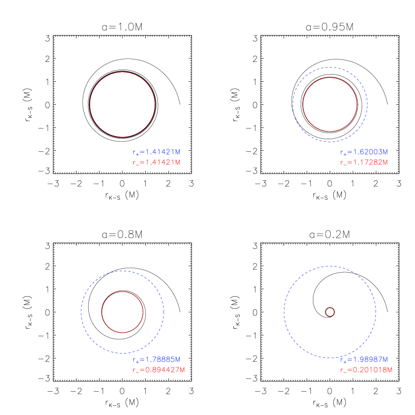
Figure 3: A ’horizon-trapped’ orbit for different values of $a$. The initial conditions for the particle are fixed and only $a$ is varied in the four orbits. The red circles represent the two horizons. It is clear that the particle successfully crosses the outer horizon and is eventually trapped at the inner horizon, except for the $a=M$ case where the two horizons coincide.

The Kerr-Schild coordinate system used in the SPH code is only avoiding the outer (future) horizon, since that serves the purpose of the SPH particles getting as close to the BH’s horizon as possible, without the code crashing or becoming problematic. Yet, in the extremal Kerr case ($a/M=1$), the two horizons coincide (Fig. 2) at $\tilde{r}=\sqrt{2}M$, and as a result, we see the orbits of the SPH particles being trapped at $\tilde{r}=\sqrt{2}M$. To check that it is the inner horizon where our transformation is singular, we set up the following simple test: we construct a test particle geodesic integrator that makes use of the K-S metric and we start with an equatorial orbit for $a/M=1$ which, starting from a finite distance from the BH (having $v_{z}=v_{y}=y=z=0$), ends being trapped at $\tilde{r}=\sqrt{2}M$. We then keep following the same orbit as we reduce the value of $a$ (Fig. 3). The result is that the particle ends being trapped at the inner horizon (whichever that is for the specific value of $a$). The trapping is illusionary: it reveals the singularity of our coordinate transformation. We thus avoid using $a/M=1$ in the simulations presented in this paper and instead we set $a/M=0.99$ for the case of an extremal Kerr B.H. By doing so, the future horizon moves outwards at $\tilde{r}_{+}=1.51067M$ and the past horizon moves inwards at $\tilde{r}_{-}=1.31067M$ and are therefore distinguishable.

Another quantity that is going to be affected by the coordinate transformation (i.e., from B-L to K-S) is the angular velocity $\Omega_{\phi}$ for a circular equatorial orbit around the BH. In B-L coordinates $\Omega_{\phi}$ is given by

$$\Omega_{\phi}=\pm\frac{M^{1/2}}{r^{3/2}\pm aM^{1/2}}$$ (25)

where $r^{2}=x^{2}+y^{2}+z^{2}$ and the upper (lower) sign corresponds to co-rotating (counter-rotating) orbits. In K-S coordinates Eq. (25) holds when $r$ is replaced by $\tilde{r}$, as defined by Eq. (16) (see Appendix C for an analytic calculation of $\Omega_{\phi}$ in K-S coordinates). In order to check this result numerically, we set up the following test: we use again the geodesic integrator and we place a test particle at some distance $r_{0}$ from the BH and give it the angular velocity that corresponds to an equatorial circular orbit at the specific $r_{0}$ as required by Eqs. (25) and (16). As expected, the test particle remains in this fixed circular orbit (with $d\tilde{r}/d\tau=0$) as we integrate for a large number of orbital periods.

2.4.2 Stable Binary Orbits

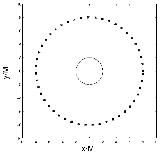
Figure 4: Test calculation for a WD orbiting a much more massive BH at $r=8\,$M. The mass ratio in this case is $q\simeq 4\times 10^{5}$. The constant radius of this circular orbit is maintained by our code to within better than $10^{-3}$ over one full period. Here each cross indicates the position of the WD (center of mass of all SPH particles) at a different time along the orbit (counter-clockwise).

In a first test, we considered a white dwarf (WD) with $M_{\ast}=0.6\,M_{\odot}$ and $R_{\ast}=1.3\times 10^{-2}\,R_{\odot}\sim 9\times 10^{8}\,$cm orbiting around a Schwarzschild BH with $M=2\times 10^{5}\,M_{\odot}$. Here $5000$ particles are used to represent the WD with a $\Gamma=5/3$ polytropic EOS. Since the mass ratio is extreme, our approximation (moving the fluid on a fixed background metric) should be extremely accurate. With these parameters, the tidal radius $R_{t}\sim 6.3\times 10^{10}$cm and the horizon scale $r_{h}=2M\sim 5.9\times 10^{10}\,$cm are comparable, and much larger than the WD radius $R_{\ast}$. If $R_{t}\gg r_{h}$, the point particle approximation should break down for orbits near the ISCO because the WD will get disrupted at radii well outside the ISCO. On the other hand, when $R_{t}\ll r_{h}$, the sound crossing time of the WD is much shorter than the orbital period, and it is numerically expensive. Thus, we have chosen the parameters satisfying $R_{t}\sim r_{h}$ to test the code for relativistic orbits. With these parameters we found that we can maintain a circular orbit at $r=8\,M$ to within $|\Delta r|/r<10^{-3}$ over one full orbital period (Fig. 4).

In a second, similar test we considered a NS with $M_{NS}=1.4\,M_{\odot}$ and $R_{NS}=13.4\,$km $=1.93\times 10^{-5}\,R_{\odot}$ (represented by $10000$ SPH particles and with a $\Gamma=2$ polytropic EOS) orbiting around a Schwarzschild BH with $M=10\,M_{\odot}$. We found that we can maintain a NS orbiting at $r=20\,M$ stably and without any noticeable numerical dissipation for more than 20 orbital periods.

2.5 Initial Conditions for BH–NS Binaries

We set up initial conditions for BH–NS binaries near the Roche limit using the SPH code and a relaxation technique similar to those used for previous SPH studies of close binaries (e.g., Rasio & Shapiro, 1995). First we construct hydrostatic equilibrium NS models for a simple gamma-law EOS by solving the Lane-Emden equation. When the NS with this hydrostatic profile is placed in orbit near a BH, spurious motions could result as the fluid responds dynamically to the sudden appearance of a strong tidal force. Instead, the initial conditions for our dynamical calculations are obtained by relaxing the NS in the presence of a BH in the co-rotating frame of the binary. For synchronized configurations (assumed here), the relaxation is done by adding an artificial friction term to the Euler equation of motion in the co-rotating frame. This forces the system to relax to a minimum-energy state. We numerically determine the angular velocity $\Omega$ corresponding to a circular orbit at a given $r$ as part of the relaxation process. The advantage of using SPH itself for setting up equilibrium solution is that the dynamical stability of these solutions can then be tested immediately by using them as initial conditions for dynamical calculations.

3 First Results

3.1 Equatorial BH–NS Mergers for Spinning and Non-spinning BH

For all the results presented in this section we ran simulations using $N=10^{4}$ SPH particles to represent a NS with a $\Gamma=2$ polytropic EOS, except for one case, for which we have performed a crude convergence test by repeating the run with $N=10^{5}$ particles (Run E1 of Table 1). The number of neighboring particles used in the SPH code is $N_{N}=80$ and $N_{N}=140$ for the low and high resolution runs, respectively. The NS mass is $M_{NS}=1.4M_{\odot}$ and its radius is $R_{NS}=15\,$km. The BH has a mass $M=15M_{\odot}$. All SPH particles are of equal mass ($m_{p}=M_{NS}/N$). The NS is initially placed at a distance $r_{0}=8M$ and for cases with a spinning BH ($a/M\neq 0$) the NS is co-rotating in the equatorial plane. The angular momentum of the BH is left as a free parameter.

In this first study we would like to get an idea of the possible outcomes of a BH–NS merger: what percentage—if any—of the NS mass survives the merger; what are the morphological features of the merger (e.g., creation of an accretion disk, spread of the accreting material), and how the BH angular momentum affects these features. For the two extreme cases $a/M=0$ and $a/M=0.99$ (we avoid using $a/M=1$ for the reasons mentioned in §2.2), we observe completely different behaviors.

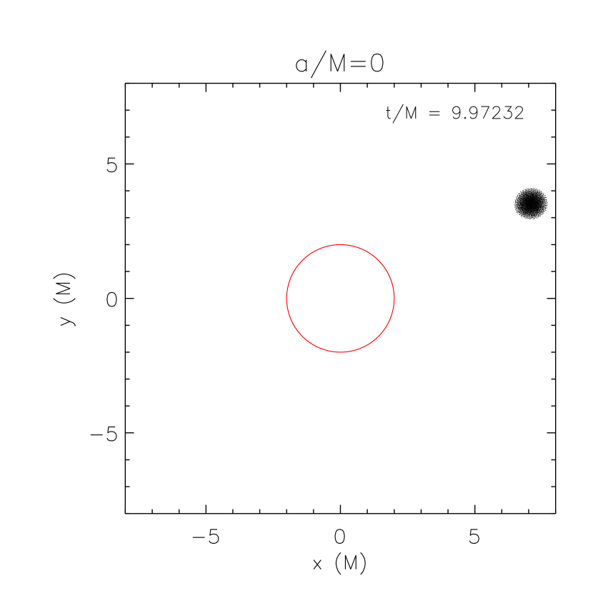
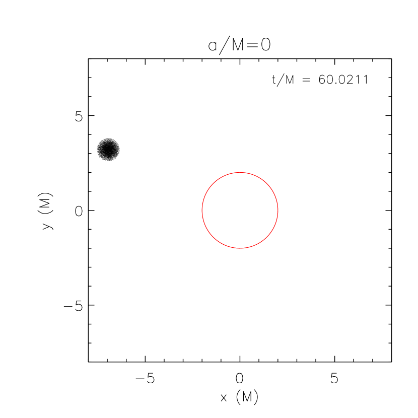
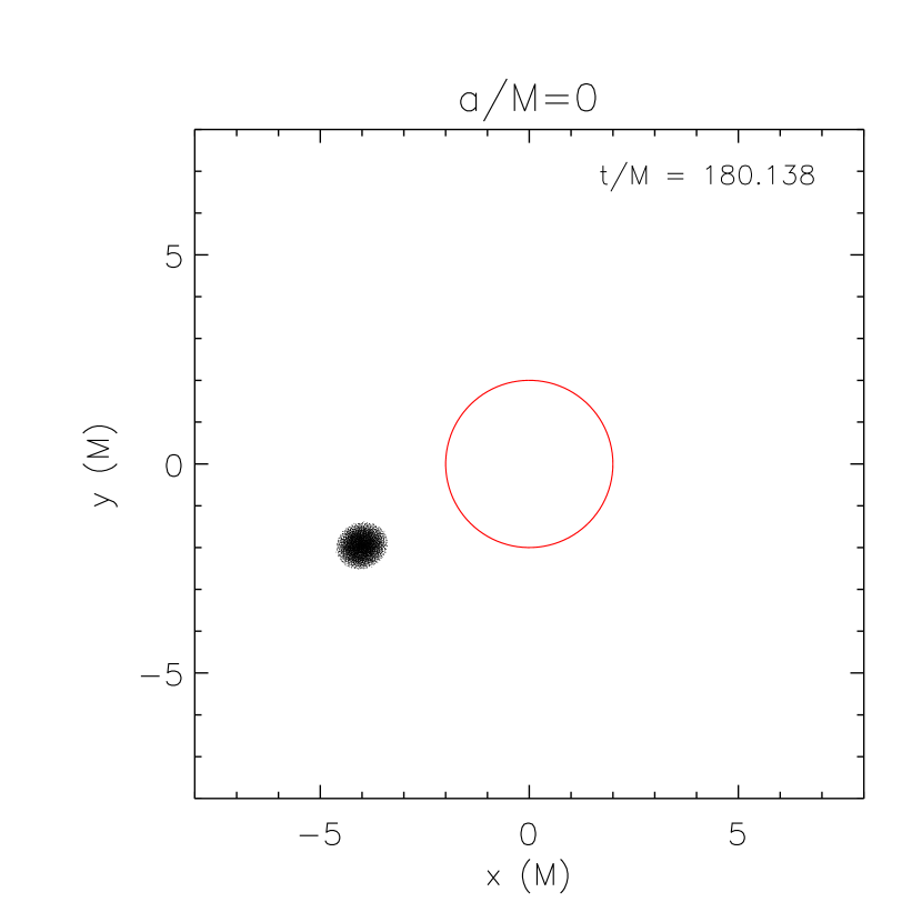
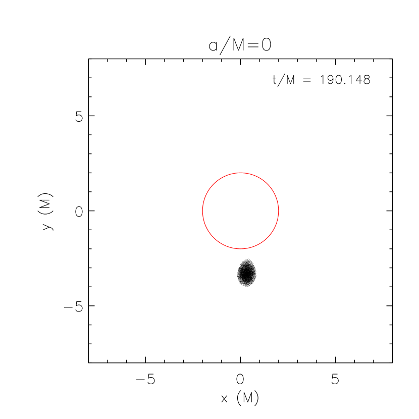
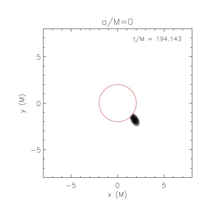
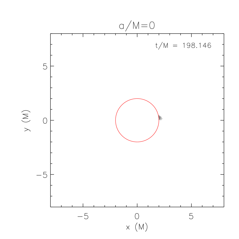
Figure 5: Sequence of six snapshots from a simulation of a non-spinning BH–NS merger (equatorial projection). The $1.4\,M_{\odot}$ NS gets completely disrupted by a non-rotating BH of mass $M=15\,M_{\odot}$. The NS was initially placed outside the tidal limit ($r\simeq 8\,M$ for this NS of radius $R\simeq 15\,$km with a $\Gamma=2$ polytropic EOS). The NS fluid is disappearing completely into the BH horizon (at $r=2M$, indicated by the red circle) in a time $t/M=180$ after the beginning of the simulation.

Fig. 5 shows the outcome of the merger for a non-spinning BH: the NS, after being completely disrupted and following an inspiraling orbit, disappears entirely into the BH’s horizon in a time $t/M\simeq 180$ after the beginning of the simulation (where $t$ is the coordinate time for an observer at inifinity).

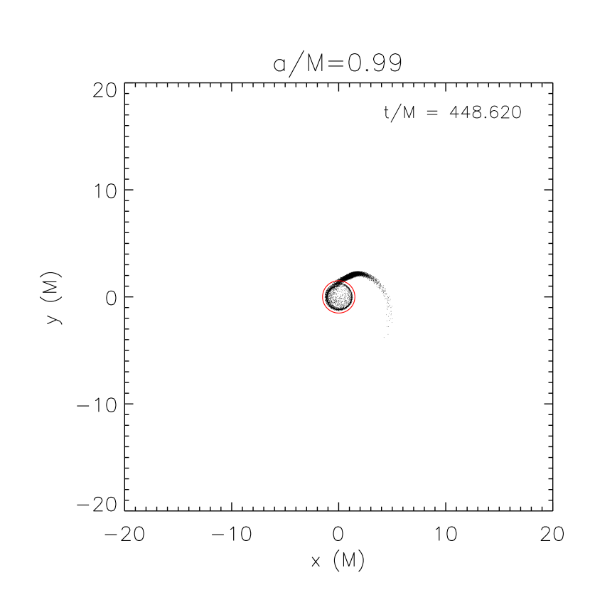
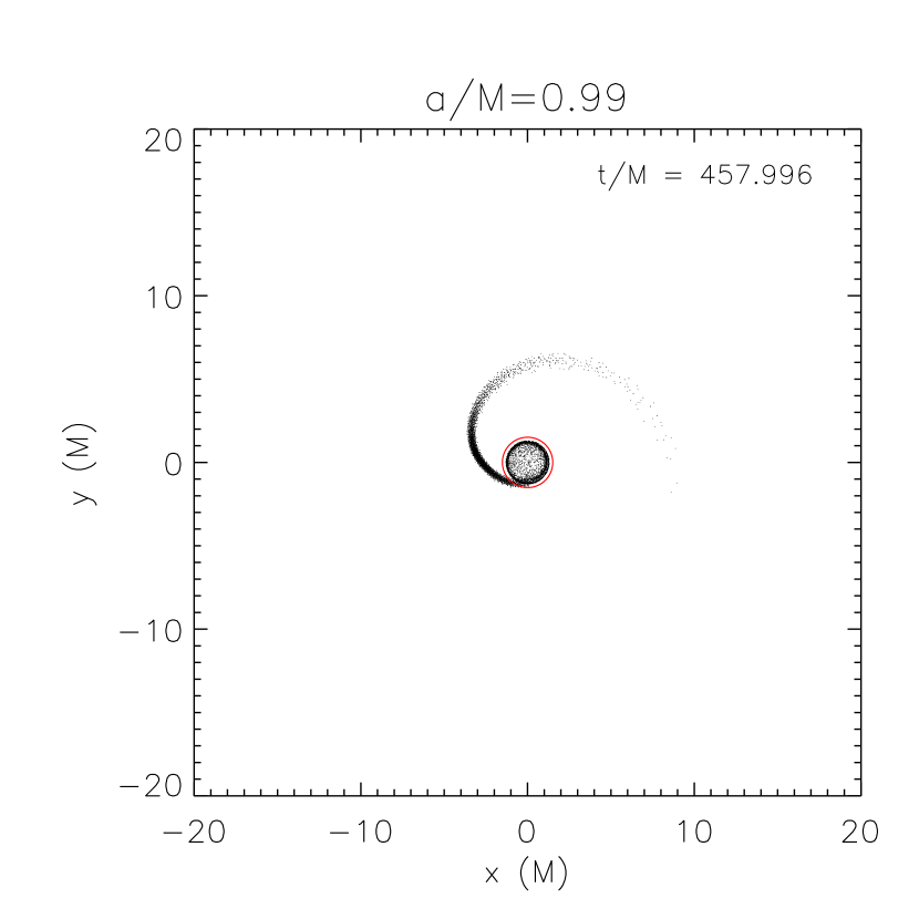
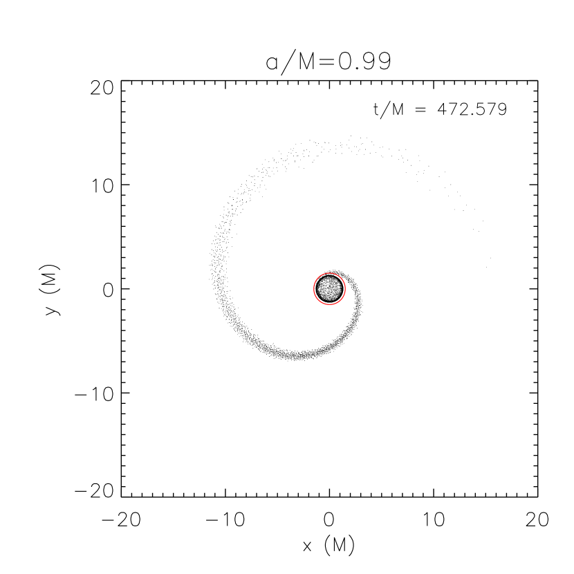
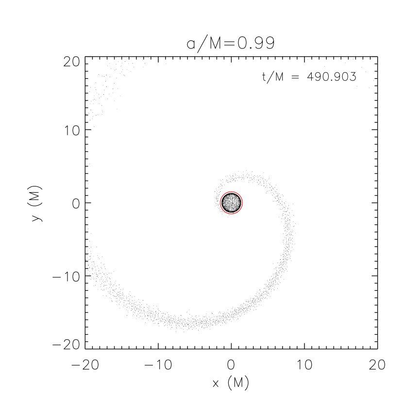
Figure 6: Same as in Fig. 5 but for a rotating BH with $a/M=0.99$. Some of the NS material is still flowing inside the BH’s horizon, but there is now also a tail of expanding material forming. By the end of the simulation ($t/M\sim 550$) the infall of material stops completely and about one third of the NS mass resides outside the horizon, with $\sim 30\%$ corresponding to unbound ejected material and the rest to the bound, disk-forming mass.

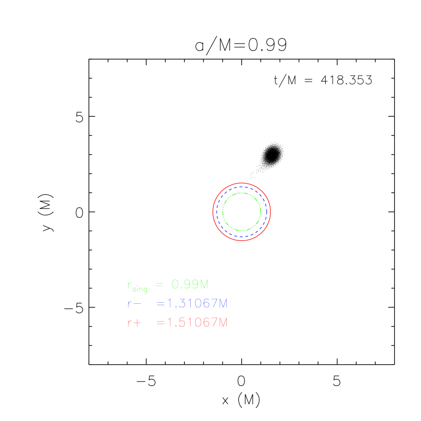
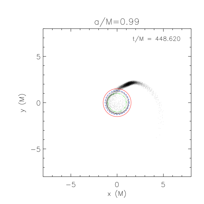
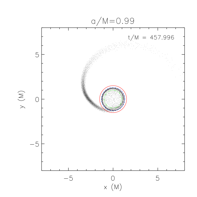
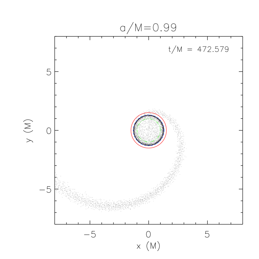
Figure 7: A close up view of the central part of four of the snapshots in Fig. 6. The three colored circles represent, in K-S coordinates, the BH’s future horizon $r_{+}$ (blue), the past horizon $r_{-}$(red) and the ring singularity at $r=a$ (green). This illustrates what we discuss in §2.1.1: the metric’s singularity at the inner (past) horizon leads to the illusory formation of a ring in the equatorial plane with radius $r=r_{-}$.

The result of our simulation for the case of the extremal Kerr BH ($a/M=0.99$) is shown in Figs. 6 and 7. The NS again gets completely disrupted and falls toward the co-rotating BH following an inspiraling orbit while an outwards expanding tail of the disrupted NS’s material is forming at the same time. The NS fluid starts disappearing into the BH’s horizon at $t/M\simeq 400$ with an initially high infall rate which finally diminishes to an almost zero level. At this point ($t/M=490$) about $33\%$ of the initial NS mass resides outside the BH’s horizon (Fig. 8). We notice that the disruption takes place well outside the ISCO, in contrast to the previous case of a Schwarzschild BH.

We run the same exact type of simulations for different values of the BH’s angular momentum and compare the results. Fig. 8 shows the fraction of the initial NS mass that survives the merger for five different values of $a/M$ ($0.75\leq a/M\leq 0.99$). As the angular momentum of the BH decreases, so does the fraction of material that survives, residing outside the BH’s horizon. For the case of $a/M=0.1$ (not included in the latter figure for practical reasons), the situation is almost the exact same as for the Schwarzschild (non-spinning) BH: the NS disappears completely into the horizon (Table 1 summarizes our results).

For the simulations with $a/M$ spanning the range $0.1<a/M<0.75$, namely for $a/M=0.2$, $a/M=0.5$ and $a/M=0.6$, we observe that the infall starts earlier as $a/M$ decreases (consistent with the behavior of the high $a/M$ mergers). No surviving material exists for those mergers with low spin for the BH ($a/M<0.7$).

The morphological features of the mergers for the non-maximally spinning BH are similar to the extremal case, with the difference that, as $a/M$ decreases the outwards expanding tail tends to spread less. For the very low $a/M$ cases no such tail is forming.

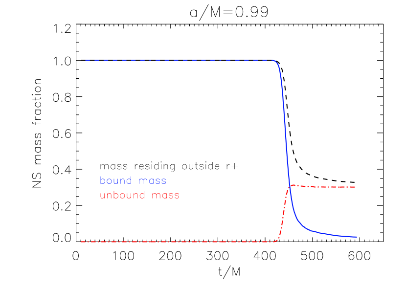
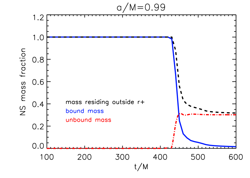
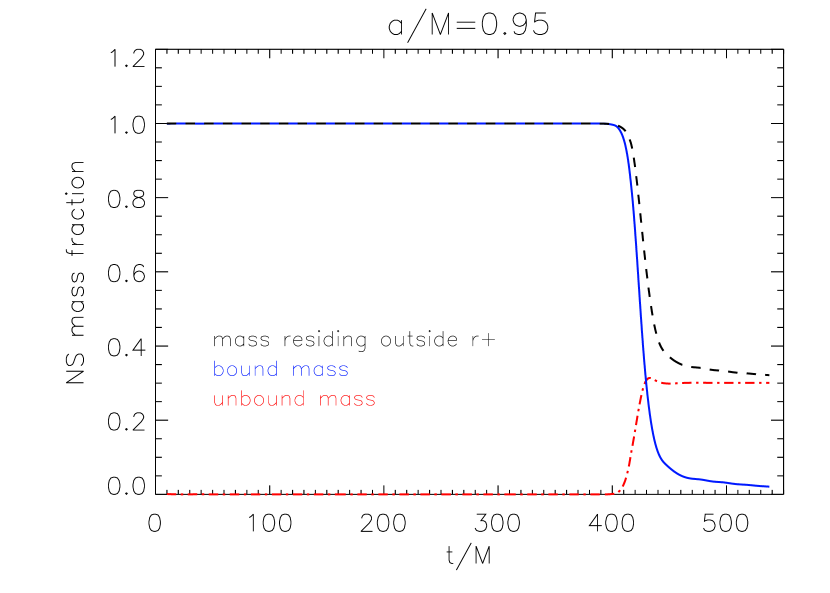
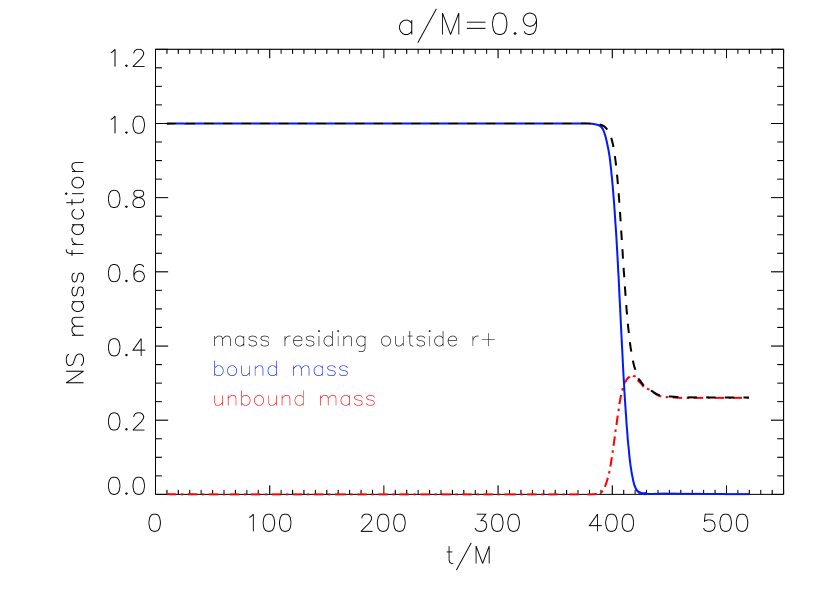
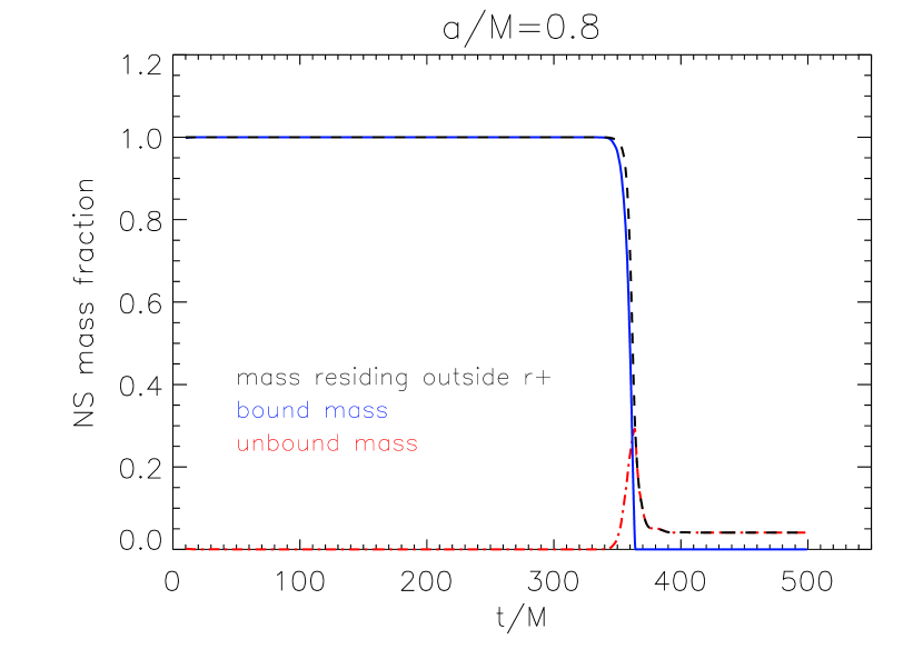
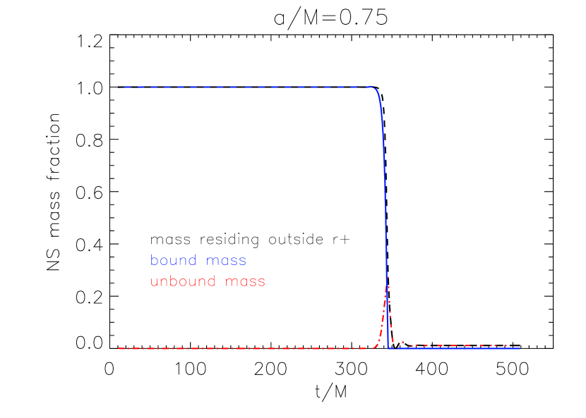
Figure 9: Fraction of the NS’s initial mass residing outside the BH’s horizon as a function of time for five different simulations, corresponding to five different values of $a/M$ (runs E1-E5). The black, blue and red lines correspond to total, bound and unbound NS material respectively. The top two plots correspond to a maximally spinning BH, using two different resolutions: $10^{4}$ and $10^{5}$ SPH particles for the left and right plots, respectively. For values of $a/M<0.95$ the percentage of surviving bound material drops to unresolvable levels.

By the end of the SPH simulations, the mass fraction that resides outside the BH’s future horizon seems to have reached a stable value. Since for $a/M\geq 0.9$ there is a substantial fraction of the NS mass surviving the merger, one would like to investigate what the final fate of this material might be, i.e., what percentage of it—if an—will escape or stay bound, forming a stable disk around the BH. To answer those questions we first calculate the rest energy (energy as measured by an observer at infinity) of each SPH particle throughout the whole simulation for runs E1-E5. By knowing a particle’s energy we can determine whether it is bound or unbound ($e^{2}>1$ for unbound and $e^{2}<1$ for bound, where $e=-(g_{tt}u^{t}+g_{t\phi}u^{\phi}+g_{tr}u^{r})$ is the energy per unit rest mass for an observer at infinity). Fig. 9 shows the variations of bound and unbound mass for each of our simulations.

For the two runs with the highest $a/M$ values (runs E1 and E2 from Table 1) we are able to resolve a nonzero fraction of bound material ($2-3\%$ of the NS mass). For runs E3, E4 and E5 the percentage of bound material drops to unresolvable values (recall that our mass resolution is $m_{p}=M_{NS}/10^{4}$). As shown in Fig. 9 for the runs E1 and E2, both the unbound and bound NS material stabilize at a certain value and persist there for a long time. That leads us to believe that the bound fraction of the surviving mass stays around the BH forming a stable disk. In order to check whether our definition of bound and unbound material is correct, we perform the following test-runs: we evolve the results of the SPH simulations using again the geodesic integrator. For every run (different $a/M$) we set as initial conditions for the geodesic integrator the last output file from the equivalent SPH simulation. We make sure to run the geodesic integrator for a sufficiently long time, as it is much faster than the SPH code. The results of those tests confirm our expectations. Namely, the material that we recognized as unbound escapes completely following parabolic trajectories, whereas the particles that were energetically determined to be bound (for runs E1 and E2 only) remain bound around the BH (and outside the BH’s horizon) following equatorial precessing orbits, with maximum apastron $\sim 30M$, minimum periastron of about $\sim 2-3M$ and a very small dispersion in the direction of the BH spin axis $\sim 0.1-0.2M$ (see Fig. 10).

Two important results are seen in Table 1: no significant fraction of bound material survives for mergers with $a/M\lesssim 0.95$ and therefore no formation of a stable disk is observed; for the cases with $a/M\lesssim 0.7$ the merger is completely catastrophic for the NS, with no material surviving.

Finally, in the upper two plots of Fig. 9 we present a comparison between a lower resolution run ($10^{4}$ particles) and a run with higher resolution ($10^{5}$ particles) for the case of a maximally spinning BH. The left panel corresponds to the low-resolution run and the right panel to the high-resolution run. The agreement between the two runs is very good and this justifies our use of the lower resolution for all runs presented in this paper. The higher-resolution run took 248 CPU hours on two dual-core AMD Opteron 2.8 GHz processors, while the lower-resolution run took only 26 CPU hours. For both cases, the simulation resulted in the ejection of about $30\%$ of the NS mass (unbound material) along with the survival of $\sim 2-3\%$ of the initial NS mass as bound material.

3.2 Non-equatorial BH–NS Mergers

Many studies have suggested that a significant NS birth kick is required for the formation of coalescing BH–NS binaries (e.g., Kalogera, 2000; Lipunov et al., 1997). Any misalignments between the axis of the BH and the NS progenitor are expected to be canceled during the evolution of the binary prior to the supernova (SN) explosion that is associated with the formation of the NS, due to mass-tranfer phases. Any spin-orbit misalignement therefore is expected to be introduced by the SN that forms the NS. Kalogera (2000) argues that tilt angles greater than $30^{o}$ are expected for $30\%-80\%$ of coalescing BH–NS binaries, whereas tilt angles of $50^{o}-100^{o}$ are expected for at most $70\%$ of such systems. In order to account for these findings, we set up some simulations for misaligned mergers, covering a wide range of tilt angles from $30^{o}-180^{o}$.

3.2.1 Setting Up Initial Conditions

The selection of initial conditions for the equatorial mergers is straight forward: select an initial radius $r_{0}$ -outside the Roche limit- and calculate the angular velocity $\Omega_{\phi}$ needed for the relaxation procedure using Eqs. (25) and (16). Obviously, Eq. (25) does not hold for non-equatorial orbits, since its derivation assumes that $\theta=\pi/2$. When moving away from the equatorial plane, there is a third constant of the motion appearing (the Carter constant $Q$), as a result of the existence of a killing tensor. (The geodesics equations of the Kerr spacetime are included in Appendix B). In order to find a stable, so-called spherical, non-equatorial orbit on which to initially place the NS, we follow the technique described in Hughes (2000). (For an in depth analysis of the procedure, refer to Hughes 2000 and Wilkins 1971). Here, we point out the basic steps for finding and setting up numerically the initial conditions for such an orbit, as presented in Hughes (2000).

For a circular orbit $R(\equiv dr/d\tau)=0=R^{\prime}$, where the prime indicates differentiation with respect to $\tau$ . Furthermore, for the orbit to be stable $R^{\prime\prime}<0$ should also hold. One can specify a unique orbit by fixing $r_{0}$ and $L_{z}$. The conditions $R=0=R^{\prime}$ will fix the other two parameters of the orbit, $E$ and $Q$. The inclination of the orbit (which is a constant of the motion) can be calculated as :

$$\cos(i)=\frac{L_{z}}{\sqrt{L_{z}^{2}+Q}}$$ (26)

(with $i$ being zero on the equatorial plane where the Carter constant $Q$ is also zero).

The most bound orbit (in terms of energy) for a given radius $r_{0}$ is the equatorial prograde orbit (in the same sense the retrograde orbit corresponds to the least-bound orbit). Therefore, one can start by choosing a radius $r_{0}$ in the equatorial plane (where $Q=0$) and then, by solving $R=0=R^{\prime}$, calculate the energy $E$ and angular momentum $L_{z}$ for that orbit. Solving analytically the condition (with $R$ being defined by Eq. (B1)) one gets for the prograde and retrograde orbits (Hughes, 2000)

$$E^{pro}=\frac{1-2v^{2}+pv^{3}}{\sqrt{1-3v^{3}+2pv^{3}}}$$ (27)

$$L_{z}^{pro}=rv\frac{1-2pv^{3}+p^{2}v^{4}}{\sqrt{1-3v^{2}+2pv^{3}}}$$ (28)

$$E^{ret}=\frac{1-2v^{2}-pv^{3}}{\sqrt{1-3v^{3}-2pv^{3}}}$$ (29)

$$L_{z}^{ret}=-rv\frac{1+2pv^{3}+p^{2}v^{4}}{\sqrt{1-3v^{2}-2pv^{3}}}$$ (30)

where $v=\sqrt{M/r}$ and $p=a/M$.

With $E$ and $L_{z}$ numerically known for a given equatorial orbit of radius $r_{0}$, one can proceed into finding non-equatorial stable orbits. The way to do so is by keeping the radius $r_{0}$ fixed, decreasing the value of $L_{z}$ and solving again for the conditions $R=0=R^{\prime}$, which now are going to give the energy and Carter constant. This way one can keep on decreasing the value of $L_{z}$ until it reaches the value $L_{z}^{ret}$ or until $R^{\prime\prime}=0$ (marginally bound). The stability of the new, inclined orbit (with the inclination given by Eq. (26)) should be checked with the requirement $R^{\prime\prime}<0$. The angular velocity of this orbit can now be numerically determined as $\Omega_{\phi}=d\phi/dt$ by using the geodesics equations for $d\phi/d\tau$ and $dt/d\tau$ (Eqs. (B3) and (B4)). The velocity for a stable, spherical, non-equatorial orbit of radius $r_{0}$ and inclination $i$ will be $v_{y}=r_{0}\Omega_{\phi}\cos(i)$

Since we have followed this numerical method to find initial conditions for the inclined mergers, tuning the $r_{0}$ and $L_{z}$ values in order to solve for an exact value of inclination angle was not trivial to do. In any case we tried to get as close to the value of the desired inclination angle as it was numerically possible. For example, the inclined merger labelled to be $30^{o}$ was in reality $29.6577^{o}$. In Table 2 we have listed the actual values of orbital inclinations used in our simulations, but when referring to them either in the text or in plot labels we use the rounded off values.

3.2.2 Results

We have run five simulations of non-equatorial mergers, for five different inclination angles all with $a/M=0.99$ (Table 2). The rest of the characteristics of the simulations presented in this section, i.e., BH and NS masses, polytropic index $\Gamma$, number of SPH particles, are as mentioned in §3.1 .

Runs I4 ($i\approx 90^{o}$) and I5 (retrograde orbit) lead to the NS being entirely lost into the BH’s horizon after spiraling around it for several orbits. The difference between the outcomes of those two mergers is that, for run I4 the feeding of the BH does not take place in the equatorial plane: the NS follows a 3-D spherical orbit of decreasing radius before it finally vanishes completely into the BH.

The outcome of Run I1 is presented in Figs. 11 and 12. As in the equatorial mergers of high $a/M$ presented in §3.1, the merger results in the formation of an expanding tail of the NS’s material, with the innermost part of the helix ’feeding’ the BH. For this case the helix does not lay on the equatorial plane , although the feeding point does. By the end of the simulation almost $40\%$ of the NS mass remains outside the BH’s horizon with most of it unbound and only about $6\%$ bound. We followed the procedure described already in §3.1 and used the geodesic integrator to further evolve the results of the SPH simulation as a test of the validity of our definition of bound and unbound mass and to check the spatial distribution of the bound material around the BH. The whole unbound part of the surviving material escapes outwards, whereas the bound mass forms a stable torus outside the BH’s horizon. Fig. 13 shows the spatial distribution of pericenters (in red - upper right and lower panels) and apocenters (in blue - upper left and middle panels) on the x-y and x-z planes. Every particle is depicted at the moment of its own apocenter (or pericenter) (i.e., those plots do not correspond to a snapshot of specific time of the equivalent merger).

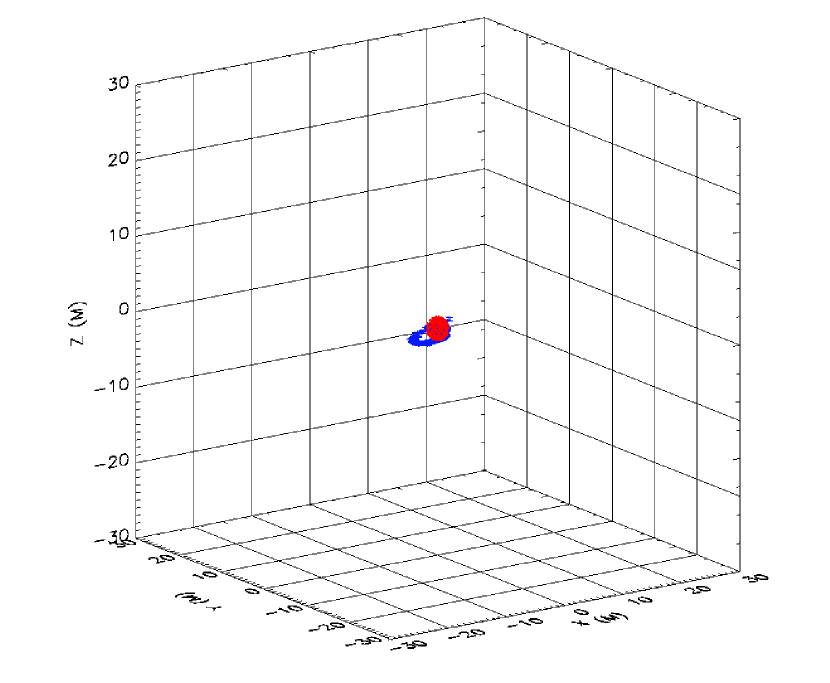
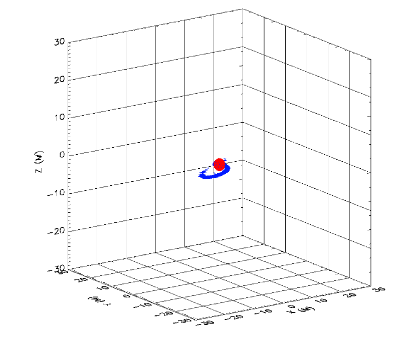
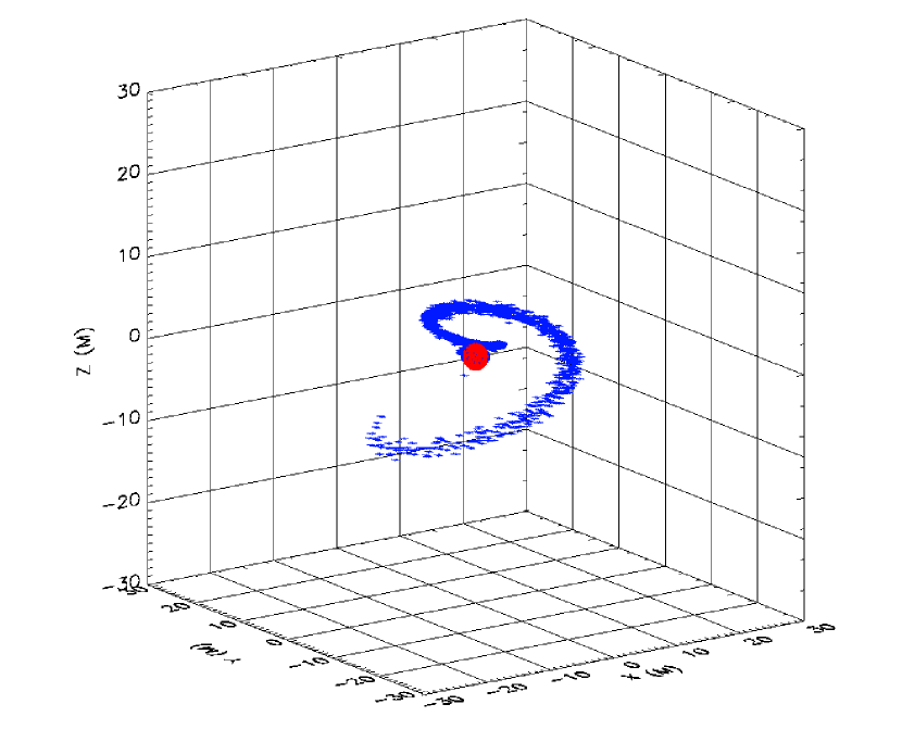
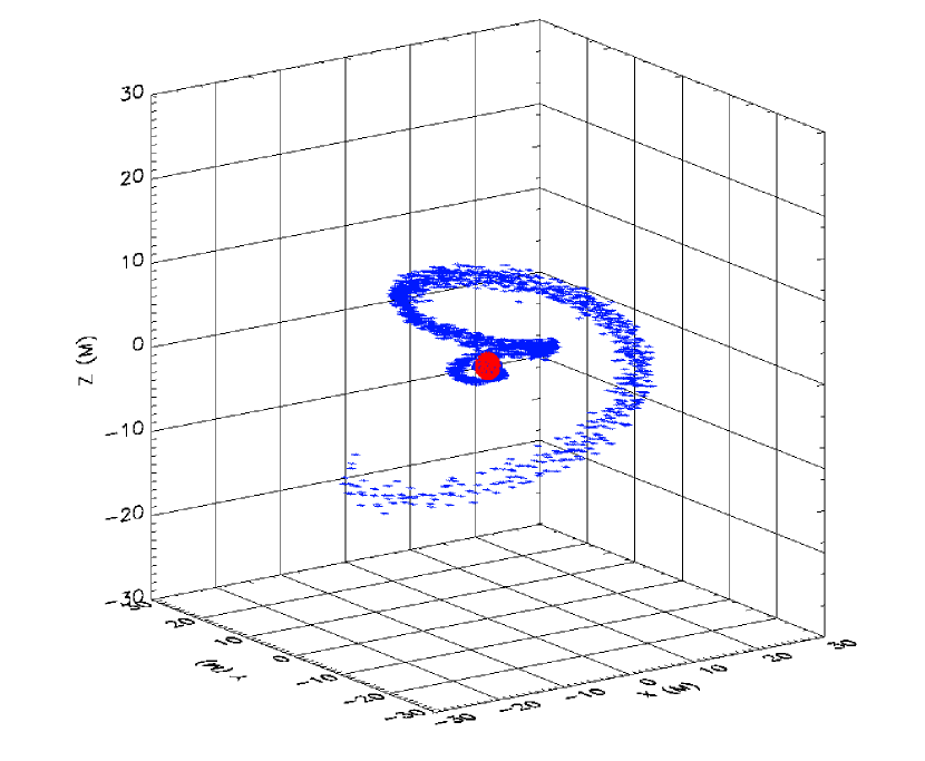
Figure 15: Four 3-D snapshots from Run I2 towards the end of the simulation. The NS has already been disrupted and starts shedding material into the BH’s horizon. An expanding helix of unbound material forms at the same time, resulting in the ejection of $25\%$ of the NS mass.

Run I2 corresponds to a merger with initial inclination of $\sim 45^{o}$. As the infall of the NS’s material into the BH starts, at about $t/M=1500$ after the beginning of the simulation, an outwards expanding tail is forming (Figs. 14 and 15) and by the end of the simulation $25\%$ of the initial NS mass (Fig. 16) is left unbound and escaping. No bound, disk-forming material was resolved in this case.

For an inclination of $\sim 70^{o}$ (Run I3) the outcome of the merger is no different than that of Runs I4 and I5: the whole NS disappears into the BH’s horizon. The morphological features of this merger, however, are somewhere in between those of the low inclination mergers, where there is material surviving outside, and the higher inclination ones, which ended up being completely catastrophic for the NS. After the NS orbits around the BH following a spherical orbit of decreasing radius, it starts accreting into the BH with the feeding point being well above the equatorial plane. As the infall continues, the part of the NS that is still outside the BH’s horizon moves towards the equatorial plane and at the last stages of the merger, when the feeding point has sufficiently approached the equatorial plane, a small, expanding, spiraling tail forms which is energetically unable to escape or expand significantly and ends up being accreted into the BH as well. At the end of the simulation there is no surviving mass (Fig. 17).

The difference between equatorial and inclined mergers in terms of the surviving bound mass seems to be the vertical (z-axis) distribution of the NS debris. In the equatorial case the bound material remains in an equatorial disk ($-0.15M\leq z\leq 0.15M$) whereas in the inclined case the disk is replaced by a torus with $-1M\leq z\leq 1M$, and this torus is also more massive than the disk in equatorial mergers.

We note that the geodesic integrator runs are taken just as an approximation and a qualitative test of the further evolution of the two groups of surviving material (bound and unbound), for the cases where hydrodynamics is of no importance and the SPH particles can be treated as free particles; e.g., for unbound particles at great distances from the BH.

4 Gravitational Wave Signals

We present here the GWs extracted for some of the simulations described in the previous section. We have used the standard quadrupole formula, in which the two polarizations of the waveform are given by

$$rh_{\times}=2\ddot{I}_{xy}$$ (31)

$$rh_{+}=\ddot{I}_{xx}-\ddot{I}_{yy}$$ (32)

where $r$ is the distance to the observer, $h_{\times}$ and $h_{+}$ the cross and plus polarization modes, and $\ddot{I}_{ij}$ the second time derivative of the second mass moment.

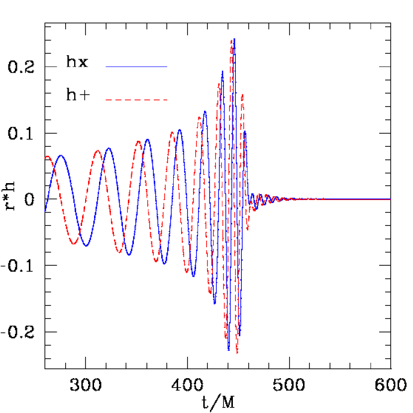
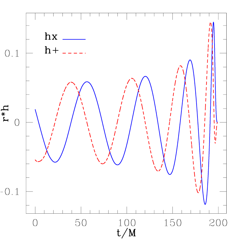
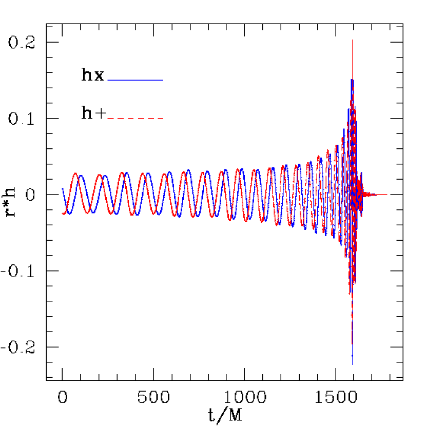
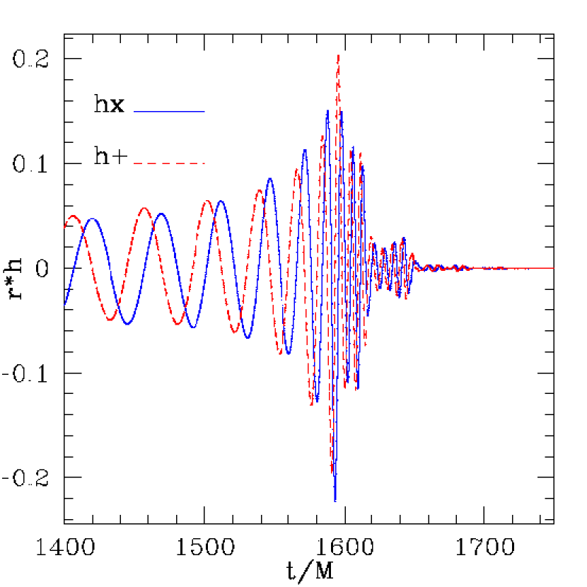
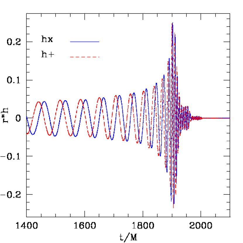
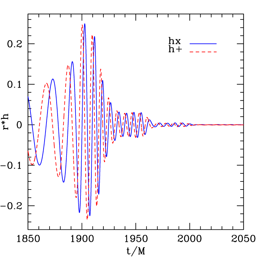
Figure 18: GW signals extracted from some of the simulations. The two upper plots correspond to runs E1 (left) and E10 (right). The middle panel plots are for run I2 with the right side showing a blowup of the left plot focussing on the later stages of the evolution. The lower panel shows the GW signal for run I1. Again the right side shows a blowup of the plot on the left.

Fig. 18 shows the GWs extracted from runs E1, E10, I2 and I1. The upper left plot corresponds to Run E1 (equatorial merger of a maximally spinning BH). As the inspiral of the NS towards the BH continues, the amplitude and frequency of the waveform is increasing, to reach its maximum just before the NS gets disrupted and starts shedding mass into the BH. From this point on, the amplitude decreases very rapidly and the signal eventually vanishes. The GWs for an equatorial merger of a non-spinning BH (run E10 in Table 1) is shown in the upper right plot of Fig. 18. Again we see the chirp signal reaching its maximum just before the NS is lost into the BH’s horizon. For a non-spinning BH the disruption of the NS is taking place very close to the horizon (as discussed above) and it just barely starts getting tidally distorted before plunging almost intact into the BH. As a result, we do not see the gradual diminishing of the wave amplitude as observed in the spinning case. The middle and lower panel plots of Fig. 18 show the GWs for Runs I2 and I1, two simulations for the merger of a maximally spinning BH with a NS set in an inclined orbit of inclination $45^{o}$ and $60^{o}$, respectively. Again we observe the characteristic chirp signal as the NS is inspiralling, with the frequency of the signal decreasing as the wave amplitude is increasing and reaches its maximum just before the NS disruption takes place. Additionally, the precession of the orbital plane is seen as a secondary chirp signal of smaller amplitude. At this point, the main core of the newly disrupted NS is found orbiting on a different plane than the rest of the NS material that has just started forming an outwards moving tail.

The GW signals shown in Fig. 18 are, at best, qualitatively correct, for two reasons. First, recall that the inspiral part of the calculations presented here is affected by the artificial strengthening of radiation reaction that we have used in order to drive the initial stages of our simulations (as described in §2.3). As a result, the early parts of the GW signals suffer a time compression that would not be present in reality. Second, the simple quadrupole formula of Eqs. 31 and 32 applies strictly to the case of a quasi-Newtonian source, while in reality the NS fluid is moving highly relativistically in the strong field region around a BH. Our intention for now is merely to provide a qualitative preview of the GW signals produced by these BH–NS mergers, and not to derive quantitatively accurate waveforms. As part of our future work we plan to develop a more sophisticated and more accurate treatment of the radiation reaction and GW extraction, which will then allow us to study in greater detail how the merger’s parameters produce distinctive features in the GW signals and energy spectrum.

5 Discussion and Summary

We have performed simulations of BH–NS mergers with mass ratio $q\simeq 0.1$ and polytropic index $\Gamma=2$ using a 3-D relativistic SPH code. We investigated equatorial mergers for various values of the BH spin and we also carried out simulations for inclined mergers (considering a tilted orbital plane for the NS with respect to the BH’s equatorial plane) in the case of an extremal Kerr BH. We find that the outcome of the merger depends strongly on the spin of the BH and the inclination of the orbit. More specifically, for equatorial mergers, the survival of NS material is possible only for mergers with $a/M>0.7$ and, in that case, the percentage of surviving material increases with increasing BH spin, varying from about $33\%$ to $\sim 1\%$ for $a/M$ decreasing from 0.99 to 0.7. Complete disruption of the NS happens for all values of $a/M$. Most of the surviving material gets ejected from the vicinity of the BH and only a few percent stays bound to the BH, forming a relatively thin stable disk outside the BH’s horizon. Only for very high BH spins ($a/M>0.95$) do we see a substantial fraction ($\sim 3\%$) of the disrupted NS material remaining bound.

The outcome of inclined mergers (for fixed $a/M=0.99$) shows strong dependence on the value of the inclination angle. For sufficiently low inclinations ($<60^{o}$) there is always a large fraction of the NS mass surviving the merger, up to $\sim 40\%$, depending on the inclination angle. Moreover, for these mergers the formation of a thick stable torus of substantial bound mass is also strongly inclination-dependent. Whenever the inclination exceeds $40-45^{o}$ the fraction of bound material drops to levels unresolvable by our present calculations, although there is still a significant fraction ($\sim 25\%$) of the material that is being ejected.

Given the sensitive dependence of our results on the BH spin, one might wonder whether the accretion of NS material onto the BH could lead to significant spin up, with a corresponding change in the spacetime metric which is not accounted for in our SPH code (where the BH spin parameter is assumed fixed during the entire evolution). For each one of the runs presented in §3 we have calculated the change in the BH spin by adding to the initial angular momentum of the BH the angular momentum of the total accreted mass (a posteriori). For Runs E1-E5 the total change in the BH spin after the accretion was less than $0.1$. More precisely, for those runs with $0.7<a/M<0.95$ the final BH was spun up by less than $0.1$, while for Runs E1 and E2 the final BH spin decreased to $a/M=0.965$ and $a/M=0.946$, respectively. Those changes are small enough that we think they would not have affected the final results of the simulations. For the runs with BH spin $0\leq a/M\leq 0.6$ the change in the final BH spin varies between $0.27$ for a non-spinning BH and $\sim 0.1$ for a BH with initial $a/M=0.6$. Even for these cases the change in the BH spin will not alter the result of the merger, as all simulations with BH spin $<0.7$ resulted in the accretion of the entire NS mass by the BH.

Another possible caveat concerns our Newtonian treatment of the NS fluid self-gravity. We should stress here the point made already in Faber et al. (2006b), that a more accurate, relativistic treatment of the NS fluid’s self-gravity could lead to even faster mass transfer to the BH, as it might result in the expansion of the NS on a dynamical scale during the mass loss phase. Although this effect could have significant impact on the outcome of some mergers, we have observed in all our simulations that the complete disruption of the NS lasts typically less than one dynamical time from the onset of mass loss and therefore we believe that the adoption of a simple Newtonian treatment of self-gravity in our code is justified.

Our findings have direct implications for the viability of BH–NS mergers as progenitors of short GRBs. The possibility of short GRBs being powered by such mergers depends on the characteristics of the binary, mainly the BH spin and the orbital inclination. Although not all BH–NS mergers seem to be promising as progenitors for short GRBs, binaries with fast spinning BHs and zero to moderate inclinations appear to form a disk or torus around the BH, massive enough to power a short GRB when later accreted by the BH. Therefore, only a fraction of BH–NS binaries could be associated with the production of short GRBs. The question of whether this fraction is high enough to explain the observed short GRBs has yet to be answered as it depends on uncertain quantities such as the BH spin and mass distributions, as well as the orbital inclination distribution for BH–NS binaries. Current population synthesis codes try to answer such questions and give better constraints on the distributions of those quantities. A recent discussion of this question in connection to short GRBs is given in Belczynski et al. (2007). The fact that the short GRB progenitors need not belong to a homogeneous group and that NS–NS binary mergers could be equally viable progenitors of short GRBs is also an open issue currently under investigation.

The complete tidal disruption of the NS in all the merger calculations that we presented in this paper is in qualitative agreement with previous Newtonian studies of BH–NS mergers with soft EOS (Rosswog et al., 2004; Lee & Kluzniak, 1999b). In our simulations that involved a Schwarzschild (non-spinning) BH, no NS material was observed being ejected or forming a disk around the BH. The accretion of the whole NS onto the BH is very prompt for this case. This is to be expected, as for the particular mass ratio ($q\simeq 0.1$) considered in our simulations the tidal limit is found inside the ISCO for $a/M=0$ and thus we would not expect to find a stable disk forming around the BH. The ejection of material and the formation of an accretion disk were observed only for mergers with highly spinning BHs.

In Paper II we will extend our simulations to include different mass ratios, although still in the limit where the use of a fixed background is justified (i.e., for BH masses much larger than the NS mass), and we will explore the effects of changing the NS EOS and relaxing our assumption of an initially synchronized NS. In this context we would like to add a brief comment about the importance of the NS EOS for the dynamics of the merger right after the disruption of the NS. Fig. 19 shows the averaged ratio of the pressure gradient forces over the gravity forces as a function of time (for the run with higher resolution presented in §3.1). We see clearly that right after the disruption of the NS (at $t/M\sim 400$) the pressure forces become insignificant and the decompressed NS material essentially follows ballistic trajectories, indicating that the details of the EOS no longer play any role. Thus one need not worry that the decompressed material should be described by a different EOS. Only the high-density EOS describing the interior of the NS prior to disruption may have a significant effect on the outcome of the merger. Ultimately, the adoption of a full numerical relativistic scheme, where no simplifying assumptions on the background spacetime metric are made, would be ideal, as it would allow us to explore mergers for binaries with higher mass ratios. Although the many Newtonian studies of these mergers have provided a qualitative overview of their possible outcomes, there is a consensus that relativistic effects will play a very significant role in the hydrodynamics of the NS disruption (as already shown by Shibata & Uryu, 2006, for the non-spinning BH case), and therefore in understanding the GW emission and the possible connection of such mergers to short GRBs.

Acknowledgments

This work was supported by NSF Grants PHY-024528 and PHY-0601995 at Northwestern University. We thank Scott Hughes and Josh Faber for useful discussions and the anonymous referee for constructive comments. PL acknowledges the support of the Center for Gravitational Wave Physics at Penn State, funded by the NSF under Cooperative Agreement PHY-0114375, and NSF grants PHY-0244788 and PHY-0555436

Appendix A K-S form of the Kerr metric

Kerr presented his solution for the first time (Kerr, 1963) in the following format

$$ds^{2}=(\tilde{r}^{2}+a^{2}\cos^{2}\theta)(d\theta^{2}+\sin^{2}\theta d\phi^{2})+2(du+a\sin^{2}\theta d\phi)\times(d\tilde{r}+a\sin^{2}\theta d\phi)$$

$$-(1-\frac{2M\tilde{r}}{\tilde{r}^{2}+a^{2}\cos^{2}\theta})\times(du+a\sin^{2}\theta d\phi)^{2}$$ (A1)

.

By using:

$$u=t+\tilde{r}$$

$$\tilde{r}\cos\theta=z$$ (A2)

$$(\tilde{r}-ia)e^{i\phi}\sin\theta=x+iy$$

Eq. (A1) can be transformed to an asymptotically flat coordinate system (Kerr, 1963).

First let’s apply $u=t+\tilde{r}$ on Eq. (A1). This will lead to the more familiar form

$$ds^{2}=-(1-\frac{2M\tilde{r}}{\Sigma})dt^{2}+(1+\frac{2M\tilde{r}}{\Sigma})d\tilde{r}^{2}+\Sigma d\theta^{2}$$

$$(\tilde{r}^{2}+a^{2}+\frac{2M\tilde{r}}{\Sigma}a^{2}\sin^{2}\theta)\sin^{2}\theta d\phi^{2}+\frac{4M\tilde{r}}{\Sigma}dt\,d\tilde{r}$$ (A3)

$$+\frac{4M\tilde{r}}{\Sigma}a\sin^{2}\theta d\phi\,dt+(1-\frac{2M\tilde{r}}{\Sigma})2a\sin^{2}\theta d\phi\,d\tilde{r}$$

where

$$\Sigma=\tilde{r}^{2}+a^{2}\cos^{2}\theta$$

and $\tilde{r}$ is defined by :

$$\tilde{r}^{4}-(\rho^{2}-a^{2})\tilde{r}^{2}-a^{2}z^{2}=0$$ (A4)

with $\rho^{2}=x^{2}+y^{2}=z^{2}$.

Now applying the rest of the transformations in (A2), one gets

$$ds^{2}=dx^{2}+dy^{2}+dz^{2}-dt^{2}+\frac{2M\tilde{r}^{3}}{\tilde{r}^{4}+a^{2}z^{2}}(k)^{2}$$ (A5)

where

$$k=[\frac{\tilde{r}(xdx+ydy)+a(xdy-udx)}{\tilde{r}^{2}+a^{2}}+\frac{z}{\tilde{r}}dz+dt].$$ (A6)

Let us make a useful parenthesis here: to understand better why the transformation rules (A2) were chosen, it is constructive to start with Eq. (A1) and bring it to the following form

$$ds^{2}=[-du^{2}+2du\,d\tilde{r}+\Sigma d\theta^{2}+2a\sin^{2}\theta d\tilde{r}\,d\phi+(\tilde{r}^{a}+a^{2})\sin^{2}\theta d\phi^{2}]$$

$$+\frac{2M\tilde{r}}{\Sigma}(du+a\sin^{2}\theta d\phi^{2}).$$ (A7)

Eq. (A7) can be interpreted as following: the terms not containing the mass m, give the flat space metric in some coordinate system, while the last term can be expressed in terms of the null (tangent with respect to $\eta_{\alpha\beta}$) vector, $l_{\alpha}$

$$-l_{\alpha}dx^{\alpha}=du+a\sin^{2}\theta d\phi$$

and therefore the line element $ds^{2}$ can be written in the form

$$ds^{2}=(ds^{2})_{flat}+\frac{2M\tilde{r}}{\Sigma}(l_{\alpha}dx^{\alpha})^{2}$$ (A8)

and the metric is

$$g_{\alpha\beta}=\eta_{\alpha\beta}+\frac{2M\tilde{r}}{\Sigma}l_{\alpha}l_{\beta}.$$ (A9)

This is actually the original way which Kerr followed to discover his solution.

The idea now is to find those transformations that will take the part of Eq. (A7) that is contained in the brackets to the standard representation of the Minkowski space. This will lead us to the already mentioned transformation rules (A2).

Notice that the metric (A5) is analytical everywhere except at $x^{2}+y^{2}=a^{2}$ (or else at $\rho=a$ and $z=0$).

Appendix B Geodesics of the Kerr spacetime in B-L coordinates

The Kerr geodesics equations (Misner, Thorne & Wheeler, 1973)

$$\Sigma^{2}\left(\frac{dr}{d\tau}\right)^{2}=[E(r^{2}+a^{2})-aL_{z}]^{2}-\Delta[r^{2}+(L_{z}-aE)^{2}+Q]\equiv R$$ (B1)

$$\Sigma^{2}\left(\frac{d\theta}{d\tau}\right)^{2}=Q-\cot^{2}\theta L_{z}^{2}-a^{2}\cos^{2}\theta(e-e^{2})\equiv\Theta$$ (B2)

$$\Sigma\left(\frac{d\phi}{d\tau}\right)=\csc^{2}\theta L_{z}+aE\left(\frac{r^{2}+a^{2}}{\Delta}-1\right)-\frac{a^{2}L_{z}}{\Delta}$$ (B3)

$$\Sigma\left(\frac{dt}{d\tau}\right)=E\left[\frac{(r^{2}+a^{2})^{2}}{\Delta}-a^{2}\sin^{2}\theta\right]+aL_{z}\left(1-\frac{r^{2}+a^{2}}{\Delta}\right)$$ (B4)

Appendix C $\Omega_{\phi}$ for equatorial orbits in K-S coordinates

The metric in K-S coordinates

$$ds^{2}=-(1-\frac{2M\tilde{r}}{\Sigma})dv^{2}+\Sigma d\theta^{2}+2dv\,d\tilde{r}-\frac{4aM\tilde{r}\sin^{2}\theta}{\Sigma}dv\,d\tilde{\phi}^{\prime}-2a\sin^{2}\theta d\tilde{r}\,d\tilde{\phi}^{\prime}$$

$$+(\tilde{r}^{2}+a^{2}+\frac{2M\tilde{r}a^{2}\sin^{2}\theta}{\Sigma})\sin^{2}\theta\,d\tilde{\phi}^{\prime 2}$$ (C1)

where

$$\tilde{r}^{4}-(x^{2}+y^{2}+z^{2}-a^{2})\tilde{r}^{2}-a^{2}z^{2}=0$$ (C2)

$$\Sigma=\tilde{r}^{2}+a^{2}\cos^{2}\theta.$$ (C3)

Restricting the metric on the $\theta=\pi/2$ plane

$$ds^{2}=-(1-\frac{2M}{\tilde{r}})dv^{2}+2dv\,d\tilde{r}-\frac{4aM}{\tilde{r}}dv\,d\tilde{\phi}^{\prime}-2ad\tilde{r}\,d\tilde{\phi}^{\prime}+(\tilde{r}^{2}+a^{2}+\frac{2Ma^{2}}{\tilde{r}})d\tilde{\phi}^{\prime 2}.$$ (C4)

Two Killing vectors are associated with the $v-$ and $\tilde{\phi}^{\prime}-$ invariance or Eq. (C4)

$$\vec{\xi}=(1,0,0,0)$$ (C5)

$$\vec{\eta}=(0,0,0,1)$$ (C6)

and the defined conserved quantities

$$e\equiv-\vec{\xi}\cdot\vec{u}$$ (C7)

$$l\equiv\vec{\eta}\cdot\vec{u}$$ (C8)

with $e$ and $l$ being the conserved energy per unit rest mass and conserved angular momentum per unit rest mass respectively. $\vec{u}$ is the four-velocity.

From Eqs. (C7) and (C8) and using $u^{\tilde{r}}=0$

$$e=-g_{vv}u^{v}-g_{v\tilde{\phi}^{\prime}}u^{\tilde{\phi}^{\prime}}$$ (C9)

$$l=g_{\tilde{\phi}^{\prime}v}u^{v}+g_{\tilde{\phi}^{\prime}\tilde{\phi}^{\prime}}u^{\tilde{\phi}^{\prime}}.$$ (C10)

From Eqs. (C9) and (C10)

$$u^{v}\equiv\frac{dv}{d\tau}=\frac{1}{\tilde{r}^{2}-2M\tilde{r}+a^{2}}[(\tilde{r}^{2}+a^{2}+\frac{2Ma^{2}}{\tilde{r}})e-\frac{2Ma}{\tilde{r}}l]$$ (C11)

$$u^{\tilde{\phi}^{\prime}}\equiv\frac{d\tilde{\phi}^{\prime}}{d\tau}=\frac{1}{\tilde{r}^{2}-2m\tilde{r}+a^{2}}[(1-\frac{2M}{\tilde{r}})l+\frac{2Ma}{\tilde{r}}e].$$ (C12)

$\Omega_{\tilde{\phi}^{\prime}}$ is defined as

$$\Omega_{\tilde{\phi}^{\prime}}\equiv\frac{d\tilde{\phi}^{\prime}/d\tau}{dv/d\tau}=\frac{(1-\frac{2M}{\tilde{r}})l/e+\frac{2Ma}{\tilde{r}}}{(\tilde{r}^{2}+a^{2}+\frac{2Ma^{2}}{\tilde{r}})-\frac{2Ma}{\tilde{r}}l/e}.$$ (C13)

We need to substitute for l/e in Eq. (C13). Heading for that we can make use of the normalization condition

$$\vec{u}\cdot\vec{u}=-1,$$ (C14)

to find

$$\frac{e^{2}-1}{2}=\frac{1}{2}\frac{d\tilde{r}}{d\tau}+[-\frac{M}{\tilde{r}}+\frac{l^{2}-a^{2}(e^{2}-1)}{2\tilde{r}^{2}}-\frac{M(l-ae)^{2}}{\tilde{r}^{3}}].$$ (C15)

Based on Eq. (C15), one can define the effective potential

$$V_{eff}=-\frac{M}{\tilde{r}}+\frac{l^{2}-a^{2}(e^{2}-1)}{2\tilde{r}^{2}}-\frac{M(l-ae)^{2}}{\tilde{r}^{3}}.$$ (C16)

For a circular orbit of radius $\tilde{r}_{0}$, the effective potential has a minimum at $\tilde{r}_{0}$

$$\frac{\vartheta V_{eff}}{\vartheta\tilde{r}}(\tilde{r}_{0})=0$$ (C17)

and also from Eq. (C15)

$$V_{eff}(\tilde{r}_{0})=\frac{e^{2}-1}{2}.$$ (C18)

From Eqs. (C17) and (C18) one can solve for $l/e$: start from Eq. (C17)

$$\frac{\vartheta V_{eff}}{\vartheta\tilde{r}}=0\Rightarrow$$

$$\tilde{r}=\frac{-a^{2}(e^{2}-1)+l^{2}+\sqrt{(a^{2}-a^{2}e^{2}+l^{2})^{2}-12(l-ae)^{2}M^{2}}}{2M}.$$ (C19)

Now, from Eqs. (C18) and (C19) solve for $l/e$

$$\frac{l}{e}=\frac{-\tilde{r}^{3/2}(a^{2}+\tilde{r}(\tilde{r}-2M))+aM^{1/2}(a^{2}+\tilde{r}(3\tilde{r}-4M))}{M^{1/2}(a^{2}M-\tilde{r}(\tilde{r}-2M)^{2}}.$$ (C20)

Substituting Eq. (C20) in Eq. (C13) will give

$$\Omega_{\tilde{\phi}^{\prime}}=\pm\frac{M^{1/2}}{\tilde{r}^{3/2}\pm aM^{1/2}}$$ (C21)

with the upper and lower signs corresponding to co-rotating and counter-rotating orbits.

Table 1: Runs and Results for Simulations of Equatorial Mergers

Run	E1	E2	E3	E4	E5	E6	E7	E8	E9	E10
a/M	0.99	0.95	0.9	0.8	0.75	0.6	0.5	0.2	0.1	0
Total NS mass outside $r_{+}$	33 %	32%	26%	4%	1%	0%	0%	0%	0%	0%
Bound NS mass outside $r_{+}$	2.5%	2%	0%	0%	0%	0%	0%	0%	0%	0%

Table 2: Initial Conditions and Results for Inclined Mergers

Run	I1	I2	I3	I4	I5
a/M	0.99	0.99	0.99	0.99	0.99
$\mathbf{r_{0}(M)}$	12	11.5	12	13	10
inclination angle (o)	29.6577	45.031	70.3989	89.9494	180
Total NS mass outside $r_{+}$	37%	25%	0%	0%	0%
Bound NS mass outside $r_{+}$	6%	0%	0%	0%	0%

Figure 1: Tidal disruption limits for a $1.4\,M_{\odot}$ NS in circular orbit around a BH of mass $M$. The radius of the ISCO is also shown for the Schwarzschild (dashed line) and maximally co-rotating Kerr cases (dash-dotted line). The two solid lines bracket the tidal limit for NS with different spins and radii (Wiggins & Lai, 2000; Lai et al., 1994). Orbits are assumed to be in the equatorial plane and prograde.

Figure 2: The future (solid blue line) and past (dashed red line) horizons of a BH for various values of the Kerr parameter $a$. The straight (dash-dotted green) line represents the ring (curvature) singularity of the K-S metric, which exists only in the equatorial plane.

Figure 8: Fraction of the NS’s initial mass that resides outside the BH’s future horizon as a function of time, for five different values of the BH’s angular momentum $a/M$ ($0.75\leq a/M\leq 0.99$). The survival of NS material outside the BH horizon depends strongly on the BH’s angular momentum. As $a/M$ decreases the fraction of surviving mass decreases as well and the merger becomes completely catastrophic for the NS for values $a/M\lesssim 0.7$. Also note that the accretion of material through the BH horizon starts earlier as the BH’s angular momentum decreases; this is to be expected as the horizon is moving further away from the BH with decreasing $a/M$.

Figure 10: Spatial distribution of the apocenters (blue) and the pericenters (red) for the disk-forming SPH particles of the $a=0.99M$ equatorial merger (Run E1). The upper left (right) and middle (bottom) panels correspond to the x-y and x-z plane projections for the apocenters (pericenters) respectively. The total mass of the disk is $2.5\%$ of the initial NS mass. The mean pericenter value (inner radius of the disk) is $r_{peri}\sim 2.5M$ and the mean apocenter (outer radius of the disk) is $r_{apo}\sim 30M$.

Figure 11: Snapshot of Run I1 (up) and its x-z projection (down) towards the end of the simulation.The red circle represents the BH’s outer horizon. The material that survives the merger forms an expanding helix. For this particular run $~{}30\%$ of the initial NS mass gets dynamically ejected and $6\%$ remains bound, forming a stable torus outside the horizon.

Figure 12: Fraction of the NS mass that resides outside the BH’s future horizon for Run I1. At time $t/M=1950$ after the beginning of the simulation, the surviving material stabilizes at $\sim 37\%$. $31\%$ corresponds to unbound escaping mass, while $6\%$ stays bound and forms a torus around the BH’s horizon.

Figure 13: Spatial distribution of the apocenters (blue) and the pericenters (red) for the bound SPH particles of Run I1. Note that in inclined mergers the bound mass forms a thick torus rather than a disk (as for equatorial mergers; compare Fig. 10). The upper left (right) and middle (bottom) panels correspond to the x-y and x-z plane projections for the apocenters (pericenters) respectively. The total mass of the torus is $6\%$ of the initial NS mass. The mean pericenter value (inner radius of the torus) is $r_{peri}\sim 2\,M$ and the mean apocenter (outer radius of the torus) is $r_{apo}\sim 25M$.

Figure 14: Snapshot from Run I2 (upper panel) and its x-z projection (lower panel) towards the end of the simulation.The red circle represents the BH’s outer horizon. By the end of the simulation an outwards expanding helix has formed, ejecting $25\%$ of the initial NS mass away from the BH. The fraction of surviving bound material was too small to be resolved in this calculation.

Figure 16: Fraction of the NS mass that resides outside the BH’s future horizon for Run I2. At time $t/M=1600$ after the beginning of the simulation, the surviving material stabilizes at $25\%$ almost all of which is unbound and therefore escaping outwards.

Figure 17: Fraction of the NS’s mass that resides outside the BH’s future horizon for Run I3. At tine $t/M=1640$ after the beginning of the simulation, the whole NS mass has crossed the BH’s outer horizon.

Figure 19: The averaged ratio of pressure gradient forces to gravitational forces as a function of time for our highest resolution run. Right after the disruption of the NS ($t/M\sim 400$) the pressure forces become negligible in comparison to the gravitational forces. As a result the fluid’s EOS plays no role anymore in the dynamics of the merger and the decompressed material follows essentially ballistic trajectories.

References

- Abbott et al. (2006) Abbott, B., et al. 2006, Phys. Rev. D, 73, 062001
- Apostolatos (1995) Apostolatos, T. A. 1995, Phys. Rev. D, 52, 605
- Arun (2006) Arun, K. G. 2006, Phys. Rev. D, 74, 024025
- Baker et al. (2007) Baker, J.G., McWilliams, S. T., van Meter, J. R., Centrella, J., Choi, D., Kelly, B. J., & Koppitz, M. 2007, Phys. Rev. D, 75, 124024
- Barthelmy et al. (2005) Barthelmy, S. D., et al. 2005, Nature, 438, 994
- Belczynski et al. (2007) Belczynski, K., Taam, R. E., Kalogera, V., Rasio, F. A., & Bulik, T. 2007, ApJ, 662, 504
- Belczynski et al. (2007) Belczynski, K., Taam, R. E., Rantsiou, E., & van der Sluys, M. 2007, (astro-ph/0703131)
- Bogdanovic et al. (2004) Bogdanovic, T., Eracleous, M., Mahadevan, S., Sirgudsson, S., & Laguna, P. 2004, ApJ, 610, 707
- Boyer-Lindquist (1967) Boyer, R.H., & Lindquist, R.W. 1967, J. of Math. Phys., 8, 265
- Buonanno et al. (2007) Buonanno, A., Cook, G., & Pretorius, F. 2007, Phys. Rev. D, 75, 14018
- Burbidge et al. (1957) Burbidge, G. R., Burbidge, W. A., Fowler, W. A., & Hoyle, F. 1957, Rev. Mod. Phys., 29, 547
- Burgay et al. (2003) Burgay, M., DAmico, N., Possenti, A., et al. 2003, Nature, 426, 531
- Burrows et al. (2006) Burrows, D., et al. 2006, ApJ, 653, 468
- Cameron (1957) Cameron, A. G. W. 1957, Pub. Astr. Soc. Pacific, 69, 201
- Chandrasekhar (1983) Chandrasekhar, S. 1983, The Mathematical Theory of Black Holes, Oxford University Press
- Dai et al. (2006) Dai, Z. G., Wang, X. Y., Wu, X. F., & Zhang, B. 2006, Science, 311, 1127
- Faber & Rasio (2000) Faber, J. A., & Rasio, F. A. 2000, Phys. Rev. D 62, 064012
- Faber et al. (2001) Faber, J. A., Rasio, F. A., & Manor, J. B. 2000, Phys. Rev. D, 63, 044012
- Faber & Rasio (2002) Faber, J. A., & Rasio, F. A. 2002, Phys. Rev. D, 65, 084042
- Faber et al. (2002) Faber, J.A., Grandclement, F., Rasio, F. A., & Taniguchi, K. 2002, Phys. Rev. Lett., 89, 231102
- Faber et al. (2006a) Faber, J. A., Baumgarte, T. W., Shapiro, S. L., & Taniguchi, K. 2006, ApJ, 641, L93
- Faber et al. (2006b) Faber, J. A., Baumgarte, T. W., Shapiro, S. L., Taniguchi, K., & Rasio, F. A. 2006, Phys. Rev. D, 73, 024012
- Fox et al. (2005) Fox, D. B., et al. 2005, Nature, 437, 845
- Frail et al. (2001) Frail, D., et al. 2001, ApJ, 562, L55
- Fryer et al. (2006) Fryer, C. L., Rockefeller, G., & Warren, M. S. 2006, ApJ, 643, 292
- Galama et al. (1998) Galama, T. J., et al. 1998, Nature, 395, 670
- Gehrels et al. (2005) Gehrels, N., et al. 2005, Nature, 437, 851
- Gehrels et al. (2006) Gehrels, N., et al. 2006, Nature, 444, 1044
- Grandclément et al. (2003) Grandclément, F., Kalogera, V., & Vecchio, A. 2003, Phys. Rev. D, 67, 042003
- Grupe et al. (2006) Grupe, D., et al. 2006, ApJ, 653, 462
- Jaikumar et al. (2006) Jaikumar, P., Meyer, B. S., Otsuki, K., & Ouyed, R. 2006, arXiv nucl-th/0610013 v1
- Janka et al. (1999) Janka, H. T., Eberl, T., Ruffert, M., & Fryer, C. L. 1999, ApJ, 527, L39
- Heitmann et al. (2005) Heitmann, K., Ricker, P. M., Warren, M. S., & Habib, S. 2005, ApJ, 160, 28
- Hjorth et al. (2003) Hjorth, J., et al. 2003, Nature, 423, 847
- Hurtle (2003) Hartle, J. B. 2003, Gravity-An Introduction to Einstein’s General Relativity,Addison Wesley
- Hughes (2000) Hughes, S. 2000, Phys. Rev. D 61, 084004
- Kalogera (2000) Kalogera, V. 2000, ApJ, 541, 319
- Kerr (1963) Kerr, R. P. 1963, Phys. Rev. Letters 11, 273
- Kim et al. (2003) Kim, C., Kalogera, V., & Lorimer, D. R. 2003, ApJ, 584, 985
- Kim et al. (2006) Kim, C., Kalogera, V., & Lorimer, D. R. 2006, (astro-ph/0608280)
- Kluzniak & Lee (1998) Kluzniak, W., & Lee, W. H. 1998, ApJ, 494, L53
- Kluzniak & Lee (2002) Kluzniak, W., & Lee, W. H. 2002, MNRAS, 335, L29
- Kobayashi et al. (2004) Kobayashi, S., Laguna, P., Phinney, E. S., & Mészáros, P. 2004, ApJ, 615, 855
- Kouveliotou et al. (1993) Kouveliotou, C., et al. 1993, ApJ, 541, L101
- Laguna et al. (1993a) Laguna, P., Miller, W. A. , & Zurek, W. H. 1993a, ApJ, 404 , L678
- Laguna et al. (1994) Laguna, P., Miller W. A., & Zurek, W. H. 1994, Mem. S.A.It. 65 1129L
- Lai et al. (1994) Lai, D., Rasio, F. A., & Shapiro, S. L. 1994, ApJ, 437, 742
- Lattimer & Schramm (1974, 1976) Lattimer, J., & Schramm, D. N. 1974, ApJ, 192, L145
- Lattimer & Schramm (1976) Lattimer, J., & Schramm, D. N. 1976, ApJ, 210, 549
- Lee & Kluzniak (1995) Lee, W. H., & Kluzniak, W. 1995, Acta Astronomica 45, 705
- Lee & Kluzniak (1999a) Lee, W. H., & Kluzniak, W. 1999, ApJ, 526, 178
- Lee & Kluzniak (1999b) Lee, W. H., & Kluzniak, W. 1999, MNRAS, 308, 780
- Lee et al. (2001) Lee, W. H., Kluzniak, W., & Nix, J. 2001, Acta Astronomica 51, 331
- Lipunov et al. (1997) Lipunov, V. M., Postnov, K. A., & Prokhorov, M. E. 1997, MNRAS, 288, 245L
- MacFadyen & Woosley (1999) MacFadyen, A. I., & Woosley, S. E. 1999, ApJ, 524, 262
- Mészáros (2006) Mészáros, P. 2006, Rep.of Prog. in Phys, 69, 2259
- Mészáros et al. (1999) Mészáros, P., Rees, M. J.,& Wijers, R.A.M.J. 1999, New Astronomy, 4, 303
- Misner, Thorne & Wheeler (1973) Misner, C. W., Thorne, K. S., & Wheeler, J. A. 1973, Gravitation, (Freeman, San Fransisco, 1973), chap.33
- Monfardini et al. (2006) Monfardini, A., et al. 2006, ApJ, 648, 1125
- Nakar (2007) Nakar, E. 2007, Phys. Rep., 442, 166
- Nelemans et al. (2001) Nelemans, G., Yungelson, L. R., & Portegies Zwart, S. F. 2001, A&A, 375, 890
- O’Shaughnessy et al. (2005) O’Shaughnessy, R., Kim, C., Fragos, T., Kalogera, V., & Belczynski, K. 2005, ApJ, 633, 1076
- O’Shaughnessy et al. (2006) O’Shaughnessy, R., Kim, C., Kalogera, V., & Belczynski, K. 2006, (astro-ph/0610076)
- Perna & Belczynski (2002) Perna, R., & Belczynski, K. 2002, ApJ, 570, 252
- Perna et al. (2006) Perna, R., Armitage, P. J., & Zhang, B. 2006, ApJ, 636, L29
- Pian et al. (2006) Pian, E., et al. 2006, Nature, 442, 1011
- Piran (2004) Piran, T. 2004, Reviews of Mod. Phys., 76, 1143
- Poisson & Will (1995) Poisson, E., & Will, C. M. 1995, Phys.Rev. D, 52, 848
- Poisson (2004) Poisson, E. 2004, A Relativist’s toolkit, (Cambridge: University Press)
- Proga & Zhang (2006) Proga, D., & Zhang, B. 2006, MNRAS, 370, L61
- Rasio & Shapiro (1995) Rasio, F. A., & Shapiro, S. L. 1995, ApJ, 438, 887
- Rosswog et al. (2004) Rosswog, S., Speith, R., & Wynn, G. A. 2004, MNRS, 351, 1121
- Rosswog (2005) Rosswog, S. 2005, ApJ, 634, 1202
- Shibata & Uryu (2007) Shibata, M., & Uryu, K. 2007, Class. Quantum Grav., 24, 125
- Shibata & Uryu (2006) Shibata, M., & Uryu, K. 2006, Phys.Rev. D, 74, 121503
- Soderberg et al. (2006) Soderberg, A., et al. 2006, ApJ, 650, 261
- Thorsett & Chakrabarty (1999) Thorsett, S. E., & Chakrabarty, D. 1999, ApJ, 512, 288
- Vallisneri (2000) Vallisneri, M. 2002, Phys. Rev. Lett., 84, 3519
- Vallisneri (2002) Vallisneri, M. 2002, in The Ninth Marcel Grossmann Meeting, ed. V. G. Gurzadyan, R. T. Jantzen, R. Ruffini , (Singapore: World Scientific Publishing), 1672V
- Villasenor et al. (2005) Villasenor, J. S., et al. 2005, Nature, 437, 855
- von Neumann & Rithmyer (1950) von Neumann, J., & Rithmyer R. D. 1950, J. Appl. Phys., 21, 232
- Warren & Salmon (1991) Warren, M. S., & Salmon, J. K. 1991, BAAS, 23.1345W
- Wiggins & Lai (2000) Wiggins, P., & Lai, D. 2000, ApJ, 532, 530
- Wilkins (1971) Wilkins, D. C., 1972, Phys. Rev. D, 5, 814
- Woosley & Bloom (2006) Woosley, S. E., & Bloom, J. S. 2006, Ann. Rev. Astron. Astrophys., 44, 507
- Zhang et al. (2006) Zhang, B., et al. 2006, ApJ, 642, 354