A 3+1 perspective on null hypersurfaces and isolated horizons

Abstract

The isolated horizon formalism recently introduced by Ashtekar et al. aims at providing a quasi-local concept of a black hole in equilibrium in an otherwise possibly dynamical spacetime. In this formalism, a hierarchy of geometrical structures is constructed on a null hypersurface. On the other side, the 3+1 formulation of general relativity provides a powerful setting for studying the spacetime dynamics, in particular gravitational radiation from black hole systems. Here we revisit the kinematics and dynamics of null hypersurfaces by making use of some 3+1 slicing of spacetime. In particular, the additional structures induced on null hypersurfaces by the 3+1 slicing permit a natural extension to the full spacetime of geometrical quantities defined on the null hypersurface. This 4-dimensional point of view facilitates the link between the null and spatial geometries. We proceed by reformulating the isolated horizon structure in this framework. We also reformulate previous works, such as Damour’s black hole mechanics, and make the link with a previous 3+1 approach of black hole horizon, namely the membrane paradigm. We explicit all geometrical objects in terms of 3+1 quantities, putting a special emphasis on the conformal 3+1 formulation. This is in particular relevant for the initial data problem of black hole spacetimes for numerical relativity. Illustrative examples are provided by considering various slicings of Schwarzschild and Kerr spacetimes.

and

1 Introduction

1.1 Scope of this article

Black holes are currently the subject of intense research, both from the observational and theoretical points of view. Numerous observations of black holes in X-ray binaries and in the center of most galaxies, including ours, have firmly established black holes as ‘standard’ objects in the astronomical field [121, 142, 126]. Moreover, black holes are one of the main targets of gravitational wave observatories which are currently starting to acquire data: LIGO [75], VIRGO [2], GEO600 [153], and TAMA [6], or are scheduled for the next decade: advanced ground-based interferometers and the space antenna LISA [115]. These vigorous observational activities constitute one of the main motivations for new theoretical developments on black holes, ranging from new quasi-local formalisms [18, 31] to numerical relativity [3, 25], going through perturbative techniques [140] and post-Newtonian ones [28]. In particular, special emphasis is devoted to the computation of the merger of inspiralling binary black holes, a not yet solved cornerstone which is par excellence the 2-body problem of general relativity, and constitutes one of the most promising sources for the interferometric gravitational wave detectors [25].

In this article, we concentrate on the geometrical description of the black hole horizon as a null hypersurface embedded in spacetime, mainly aiming at numerical relativity applications. Let us recall that a null hypersurface is a 3-dimensional surface ruled by null geodesics (i.e. light rays), like the light cone in Minkowski spacetime, and that it is always a “one-way membrane”: it divides locally spacetime in two regions, $A$ and $B$ let’s say, such that any future directed causal (i.e. null or timelike) curve can move from region $A$ to region $B$, but not in the reverse way. Regarding black holes, null hypersurfaces are relevant in two contexts. Firstly, wherever it is smooth, the black hole event horizon is a null hypersurface of spacetime [39, 40, 48] . Let us stress that the event horizon constitutes an intrinsically global concept, in the sense that its definition requires the knowledge of the whole spacetime (to determine whether null geodesics can reach null infinity). Secondly, a systematic attempt to provide a quasi-local description of black holes has been initiated in the recent years by Hayward [93, 94] (concept of future trapping horizons) and Ashtekar and collaborators [10, 11, 12, 13, 14, 15, 16, 17] (see Refs. [18, 31] for a review) (concepts of isolated and dynamical horizons). Restricted to the quasi-equilibrium case (isolated horizons), the quasi-local description amounts to model the black hole horizon by a null hypersurface. This line of research finds its motivations and subsequent applications in a variety of fields of gravitational physics such as black hole mechanics, mathematical relativity, quantum gravity and, due to its quasi-local character, numerical relativity [65, 108, 99, 58, 19].

The geometry of a null hypersurface ${\mathcal{H}}$ is usually described in terms of objects that are intrinsic to ${\mathcal{H}}$. At least some of them admit no natural extension outside the hypersurface ${\mathcal{H}}$. In the case of the isolated horizon formalism this leads, in a natural way, to a discussion which is eminently intrinsic to ${\mathcal{H}}$ in a twofold manner. On one hand, the derived expressions are generically valid only on ${\mathcal{H}}$ without canonical extensions to a neighbourhood of the surrounding spacetime. On the other hand, since in this setting the hypersurface ${\mathcal{H}}$ can be seen as representing the history of a spacelike 2-sphere (a world-tube in spacetime), the study of ${\mathcal{H}}$’s geometry from a strictly intrinsic point of view leads to a strategy in which one firstly discuss evolution concepts, and then one considers the initial conditions on the 2-sphere which are compatible with such an evolution. We may call this an up-down strategy.

On the contrary, the dynamics of black hole spacetimes is mostly studied within the 3+1 formalism (see e.g. [25, 171] for a review), which amounts in the foliation of spacetime by a family of spacelike hypersurfaces. In this case, one deals with a Cauchy problem, starting from some initial spacelike hypersurface $\Sigma_{0}$ and evolving it in order to construct the proper spacetime objects. In particular, this applies to the construction of the horizon ${\mathcal{H}}$ as a worldtube. We may call this a down-up strategy.

In this article, we analyse the dynamics of null hypersurfaces from the 3+1 point of view. As a methodological strategy, we adopt a complete 4-dimensional description, even when considering objects which are actually intrinsic to a given (hyper)surface. This facilitates the link between the null horizon hypersurface and the spatial hypersurfaces of the 3+1 slicing. Moreover, the 3+1 foliation of spacetime induces an additional structure on ${\mathcal{H}}$ which allows to normalize unambiguously the null normal to ${\mathcal{H}}$ and to define a projector onto ${\mathcal{H}}$. Let us recall that a distinctive feature of null hypersurfaces is the lack of such canonical constructions, contrary to the spacelike or timelike case where one can unambiguously define the unit normal vector and the orthogonal projector onto the hypersurface.

Null hypersurfaces have been extensively studied in the literature in connection with black hole horizons, from many different points of view. In the seventies, Háj́iček conducted geometrical studies of non-expanding null hypersurfaces to model stationary black hole horizons [82, 83, 84]. By studying the response of the (null) event horizon to external perturbations, Hawking and Hartle [91, 85, 86] introduced the concept of black hole viscosity. This hydrodynamical analogy was extended by Damour [59, 60, 61]. Electromagnetic aspects were studied by Damour [59, 60, 61] and Znajek [175, 176]. These studies led to the famous membrane paradigm for the description of black holes ([141, 165] and references therein). In particular, this paradigm represents the first systematic 3+1 approach to black hole physics. Whereas these studies all dealt with the event horizon (the global aspect of a black hole), a quasi-local approach, based on the notion of trapped surface [132], has been initiated in the nineties by Hayward [93, 94], in the framework of the 2+2 formalism. Closely related to these ideas, a systematic quasi-local treatment has been developed these last years by Ashtekar and collaborators [10, 11, 12, 13, 14, 15, 16, 17] (see Refs. [18, 31] for a review), giving rise to the notion of isolated horizons and more recently to that of dynamical horizons, the latter not being constructed on a null hypersurface, but on a spacelike one.

One purpose of this article is to fill the gap existing between the mathematical techniques used in null geometry and the standard expertise in the numerical relativity community. Consequently, an important effort will be devoted to the derivation of explicit expressions of null-geometry quantities in terms of 3+1 objects. More generally, the article is relatively self-contained, and requires only an elementary knowledge of differential geometry, at the level of introductory textbooks in general relativity [90, 123, 167]. We have tried to be quite pedagogical, by providing concrete examples and detailed derivations of the main results. In fact, these explicit developments permit to access directly to intermediate steps, which might be useful in actual numerical implementation. We rederive the basic properties of null hypersurfaces, taking advantage of our 3+1 perspective, namely the unambiguous definition of the null normal and transverse projector provided by the 3+1 spacelike slicing. Therefore the present article should not be considered as a substitute for comprehensive formal presentations of the intrinsic geometry of null surfaces, as Refs. [73, 72, 109, 101, 103]. Likewise, it is not the aim here to review the isolated horizon formalism and its applications, something already carried out in a full extent in Ref. [18].

Despite the length of the article, some important topics are not treated here, namely electromagnetic properties of black holes or black hole thermodynamics. In particular, we will not develop the Hamiltonian description of black hole mechanics in the isolated horizon scheme, except for the minimum required to discuss the physical parameters associated with the black hole. We do not comment either on the application of the isolated horizon framework beyond Einstein-Maxwell theory to include, e.g. Yang-Mills fields. Even though these fields are not expected to be significant in an astrophysical setting, their inclusion involves a major conceptual and structural interest; we refer the reader to chapter 6 in Ref. [18] for a review on the achievements in this line of research, namely on the mass of solitonic solutions.

The plan of the article is as follows. After setting the notations in the next subsection, we start by reviewing the basic properties of null hypersurfaces in Sec. 2. Then the spacelike slicing of the 3+1 formalism widely used in numerical relativity is introduced in Sec. 3. The additional structures induced by this slicing on a given null hypersurface ${\mathcal{H}}$ are discussed in Sec. 4; in particular, this involves a privileged null normal, a null transverse vector and the associated projector onto ${\mathcal{H}}$. Equipped with these tools, we proceed in Sec. 5 to describe the kinematics of null hypersurfaces, namely relations involving the first “time” derivative of their degenerate metric. The next logical step corresponds to dynamics, namely the second order derivatives of the metric, which is explored in Sec. 6. The Einstein equation naturally enters the scene at this level. In particular, we recover in Sec. 6 previous results from the membrane paradigm, like Damour’s Navier-Stokes equation or the tidal-force equation. Then in Sec. 7 we move to the quasi-local approach of black holes by restricting to null hypersurfaces with vanishing expansion, which are the “perfect horizons” of Háj́iček and constitute the first step in Ashtekar et al. hierarchy leading to isolated horizons. The next levels in the hierarchy are studied in Secs. 8 and 9, where we discuss the weakly and strongly isolated horizon structures. Due to the extension of the material, these two sections rely more explicitly on the existing literature and, as a consequence, the intrinsic point of view of the geometry of ${\mathcal{H}}$ (the up-down strategy referred above) acquires there a more important role than in the rest of the article. In Sec. 10, we express basic objects of null geometry in terms of the 3+1 quantities, including the standard conformal decompositions of 3+1 objects. This allows to translate in Sec. 11 the isolated horizon prescriptions into boundary conditions for the relevant 3+1 fields on some excised sphere, making the link with numerical relativity. Some technical details are treated in appendices: the relationship between different derivatives along the null normal is given Appendix A; Appendix B is devoted to the complete computation of the spacetime Riemann tensor. In contrast with some works on null hypersurfaces, we do not make use of the Newman-Penrose formalism but rely instead on Cartan’s structure equations. Appendix C briefly presents, with the aid of examples, the basics of the Hamiltonian description. Appendix D provides the concrete example of the horizon of a Kerr black hole, while simpler examples, based on Minkowski or Schwarzschild spacetimes, are provided throughout the main text. Finally Appendix E gathers the different symbols used throughout the article.

1.2 Notations and conventions

For the benefit of the reader, we give here a somewhat detailed exposure of the notations used throughout the article. This is also the occasion to recall some concepts from elementary differential geometry employed in the article.

We consider a spacetime $({\mathcal{M}},\bm{g})$ where ${\mathcal{M}}$ is a real smooth (i.e. $\mathcal{C}^{\infty}$) manifold of dimension 4 and $\bm{g}$ a Lorentzian metric on ${\mathcal{M}}$, of signature $(-,+,+,+)$. We denote by $\bm{\nabla}$ the affine connection associated with $\bm{g}$, and call it the spacetime connection to distinguish it from other connections introduced in the text.

At a given point $p\in{\mathcal{M}}$, we denote by ${\mathcal{T}}_{p}({\mathcal{M}})$ the tangent space, i.e. the (4-dimensional) space of vectors at $p$. Its dual space (also called cotangent space) is denoted by ${\mathcal{T}}_{p}^{*}({\mathcal{M}})$ and is constituted by all linear forms at $p$. We denote by ${\mathcal{T}}({\mathcal{M}})$ (resp. ${\mathcal{T}}^{*}({\mathcal{M}})$) the space of smooth vector fields (resp. 1-forms) on ${\mathcal{M}}$. The experienced reader is warned that ${\mathcal{T}}({\mathcal{M}})$ does not stand for the tangent bundle of ${\mathcal{M}}$ (it rather corresponds to the space of smooth cross-sections of that bundle). No confusion may arise since we shall not use the notion of bundle in this article.

1.2.1 Tensors: ‘index’ notation versus ‘intrinsic’ notation

Since we will manipulate geometrical quantities which are not well suited to the index notation (like Lie derivatives or exterior derivatives), we will use quite often an index-free notation. When dealing with indices, we adopt the following conventions: all Greek indices run in $\{0,1,2,3\}$. We will use letters from the beginning of the alphabet ($\alpha$, $\beta$, $\gamma$, …) for free indices, and letters starting from $\mu$ ($\mu$, $\nu$, $\rho$, …) as dumb indices for contraction (in this way the tensorial degree (valence) of any equation is immediately apparent). All capital Latin indices ($A$, $B$, $C$, …) run in $\{0,2,3\}$ and lower case Latin indices starting from the letter $i$ ($i$, $j$, $k$, …) run in $\{1,2,3\}$, while those starting from the beginning of the alphabet ($a$, $b$, $c$, …) run in $\{2,3\}$ only.

For the sake of clarity, let us recall that if $(\bm{e}_{\alpha})$ is a vector basis of the tangent space ${\mathcal{T}}_{p}({\mathcal{M}})$ and $(\bm{e}^{\alpha})$ is the associate dual basis, i.e. the basis of ${\mathcal{T}}_{p}^{*}({\mathcal{M}})$ such that $\bm{e}^{\alpha}(\bm{e}_{\beta})=\delta^{\alpha}_{\ \,\beta}$, the components $T^{\alpha_{1}\ldots\alpha_{p}}_{\qquad\ \;\beta_{1}\ldots\beta_{q}}$ of a tensor $\bm{T}$ of type $\left({p\atop q}\right)$ with respect to the bases $(\bm{e}_{\alpha})$ and $(\bm{e}^{\alpha})$ are given by the expansion

$$\bm{T}=T^{\alpha_{1}\ldots\alpha_{p}}_{\qquad\ \;\beta_{1}\ldots\beta_{q}}\;\bm{e}_{\alpha_{1}}\otimes\ldots\otimes\bm{e}_{\alpha_{p}}\otimes\bm{e}^{\beta_{1}}\otimes\ldots\otimes\bm{e}^{\beta_{q}}.$$ (1.1)

The components $\nabla_{\gamma}T^{\alpha_{1}\ldots\alpha_{p}}_{\qquad\ \;\beta_{1}\ldots\beta_{q}}$ of the covariant derivative $\bm{\nabla}\bm{T}$ are defined by the expansion

$$\bm{\nabla}\bm{T}=\nabla_{\gamma}\,T^{\alpha_{1}\ldots\alpha_{p}}_{\qquad\ \;\beta_{1}\ldots\beta_{q}}\;\bm{e}_{\alpha_{1}}\otimes\ldots\otimes\bm{e}_{\alpha_{p}}\otimes\bm{e}^{\beta_{1}}\otimes\ldots\otimes\bm{e}^{\beta_{q}}\otimes\bm{e}^{\gamma}.$$ (1.2)

Note the position of the “derivative index” $\gamma$ : $\bm{e}^{\gamma}$ is the last 1-form of the tensorial product on the right-hand side. In this respect, the notation $T^{\alpha_{1}\ldots\alpha_{p}}_{\qquad\ \;\beta_{1}\ldots\beta_{q};\gamma}$ instead of $\nabla_{\gamma}\,T^{\alpha_{1}\ldots\alpha_{p}}_{\qquad\ \;\beta_{1}\ldots\beta_{q}}$ would have been more appropriate . This index convention agrees with that of MTW [123] [cf. their Eq. (10.17)]. As a result, the covariant derivative of the tensor $\bm{T}$ along any vector field $\bm{u}$ is related to $\bm{\nabla}\bm{T}$ by

$$\bm{\nabla}_{\bm{u}}\bm{T}=\bm{\nabla}\bm{T}(\underbrace{.,\ldots,.}_{p+q\ {\rm slots}},\bm{u}).$$ (1.3)

The components of $\bm{\nabla}_{\bm{u}}\bm{T}$ are then $u^{\mu}\nabla_{\mu}T^{\alpha_{1}\ldots\alpha_{p}}_{\qquad\ \;\beta_{1}\ldots\beta_{q}}$.

Given a vector field $\bm{v}$ on ${\mathcal{M}}$, the infinitesimal change of any tensor field $\bm{T}$ along the flow of $\bm{v}$, is given by the Lie derivative of $\bm{T}$ with respect to $\bm{v}$, denoted by $\bm{\mathcal{L}}_{\bm{\bm{v}}}\,\bm{T}$ and whose components are

$$({\mathcal{L}}_{\bm{v}}\,T)^{\alpha_{1}\ldots\alpha_{p}}_{\qquad\ \;\beta_{1}\ldots\beta_{q}} = v^{\mu}\nabla_{\mu}\,T^{\alpha_{1}\ldots\alpha_{p}}_{\qquad\ \;\beta_{1}\ldots\beta_{q}}$$

$$- \sum_{i=1}^{p}T^{\alpha_{1}\ldots\mu\ldots\alpha_{p}}_{\qquad\ \ \ \ \;\beta_{1}\ldots\beta_{q}}\nabla_{\mu}v^{\alpha_{i}}+\sum_{i=1}^{q}T^{\alpha_{1}\ldots\alpha_{p}}_{\qquad\ \;\beta_{1}\ldots\mu\ldots\beta_{q}}\nabla_{\beta_{i}}v^{\mu}\ ,$$

where the connection $\bm{\nabla}$ can be substituted by any other torsion-free connection. Actually let us recall that the Lie derivative depends only upon the differentiable structure of the manifold ${\mathcal{M}}$ and not upon the metric $\bm{g}$ nor a particular affine connection. In this article, extensive use will be made of expression (1.2.1), as well as of its straightforward analogues on submanifolds of ${\mathcal{M}}$ (see also Appendix A).

We denote the scalar product of two vectors with respect to the metric $\bm{g}$ by a dot:

$$\forall(\bm{u},\bm{v})\in{\mathcal{T}}_{p}({\mathcal{M}})\times{\mathcal{T}}_{p}({\mathcal{M}}),\quad\bm{u}\cdot\bm{v}:=\bm{g}(\bm{u},\bm{v}).$$ (1.5)

We also use a dot for the contraction of two tensors $\bm{A}$ and $\bm{B}$ on the last index of $\bm{A}$ and the first index of $\bm{B}$ (provided of course that these indices are of opposite types). For instance if $\bm{A}$ is a bilinear form and $\bm{B}$ a vector, $\bm{A}\cdot\bm{B}$ is the linear form which components are

$$(A\cdot B)_{\alpha}=A_{\alpha\mu}B^{\mu}.$$ (1.6)

However, to denote the action of linear forms on vectors, we will use brackets instead of a dot:

$$\forall(\bm{\omega},\bm{v})\in{\mathcal{T}}_{p}^{*}({\mathcal{M}})\times{\mathcal{T}}_{p}({\mathcal{M}}),\quad\langle\bm{\omega},\bm{v}\rangle=\bm{\omega}\cdot\bm{v}=\omega_{\mu}\,v^{\mu}.$$ (1.7)

Given a 1-form $\bm{\omega}$ and a vector field $\bm{u}$, the directional covariant derivative $\bm{\nabla}_{\bm{u}}\,\bm{\omega}$ is a 1-form and we have [combining the notations (1.7) and (1.3)]

$$\forall(\bm{\omega},\bm{u},\bm{v})\in{\mathcal{T}}^{*}({\mathcal{M}})\times{\mathcal{T}}({\mathcal{M}})\times{\mathcal{T}}({\mathcal{M}}),\quad\langle\bm{\nabla}_{\bm{u}}\,\bm{\omega},\bm{v}\rangle=\bm{\nabla}\bm{\omega}(\bm{v},\bm{u}).$$ (1.8)

Again, notice the ordering in the arguments of the bilinear form $\bm{\nabla}\bm{\omega}$. Taking the risk of insisting outrageously, let us stress that this is equivalent to say that the components $(\nabla\omega)_{\alpha\beta}$ of $\bm{\nabla}\bm{\omega}$ with respect to a given basis $(\bm{e}^{\alpha}\otimes\bm{e}^{\beta})$ of ${\mathcal{T}}^{*}({\mathcal{M}})\otimes{\mathcal{T}}^{*}({\mathcal{M}})$ are $\nabla_{\beta}\omega_{\alpha}$:

$$\bm{\nabla}\bm{\omega}=\nabla_{\beta}\omega_{\alpha}\;\bm{e}^{\alpha}\otimes\bm{e}^{\beta},$$ (1.9)

this relation constituting a particular case of Eq. (1.2).

The metric $\bm{g}$ induces an isomorphism between ${\mathcal{T}}_{p}({\mathcal{M}})$ (vectors) and ${\mathcal{T}}_{p}^{*}({\mathcal{M}})$ (linear forms) which, in the index notation, corresponds to the lowering or raising of the index by contraction with $g_{\alpha\beta}$ or $g^{\alpha\beta}$. In the present article, an index-free symbol will always denote a tensor with a fixed covariance type (e.g. a vector, a 1-form, a bilinear form, etc…). We will therefore use a different symbol to denote its image under the metric isomorphism. In particular, we denote by an underbar the isomorphism ${\mathcal{T}}_{p}({\mathcal{M}})\rightarrow{\mathcal{T}}_{p}^{*}({\mathcal{M}})$ and by an arrow the reverse isomorphism ${\mathcal{T}}_{p}^{*}({\mathcal{M}})\rightarrow{\mathcal{T}}_{p}({\mathcal{M}})$:

1. for any vector $\bm{u}$ in ${\mathcal{T}}_{p}({\mathcal{M}})$, $\underline{\bm{u}}$ stands for the unique linear form such that

   $$\forall\bm{v}\in{\mathcal{T}}_{p}({\mathcal{M}}),\quad\langle\underline{\bm{u}},\bm{v}\rangle=\bm{g}(\bm{u},\bm{v}).$$ (1.10)

   However, we will omit the underlining on the components of $\underline{\bm{u}}$, since the position of the index allows to distinguish between vectors and linear forms, following the standard usage: if the components of $\bm{u}$ in a given basis $(\bm{e}_{\alpha})$ are denoted by $u^{\alpha}$, the components of $\underline{\bm{u}}$ in the dual basis $(\bm{e}^{\alpha})$ are then denoted by $u_{\alpha}$ [in agreement with Eq. (1.1)].

2. for any linear form $\bm{\omega}$ in ${\mathcal{T}}_{p}^{*}({\mathcal{M}})$, $\vec{\bm{\omega}}$ stands for the unique vector of ${\mathcal{T}}_{p}({\mathcal{M}})$ such that

   $$\forall\bm{v}\in{\mathcal{T}}_{p}({\mathcal{M}}),\quad\bm{g}(\vec{\bm{\omega}},\bm{v})=\langle\bm{\omega},\bm{v}\rangle.$$ (1.11)

   As for the underbar, we will omit the arrow over the components of $\vec{\bm{\omega}}$ by denoting them $\omega^{\alpha}$.

3. we extend the arrow notation to bilinear forms on ${\mathcal{T}}_{p}({\mathcal{M}})$: for any bilinear form $\bm{T}\,:\,{\mathcal{T}}_{p}({\mathcal{M}})\times{\mathcal{T}}_{p}({\mathcal{M}})\rightarrow\mathbb{R}$, we denote by $\vec{\bm{T}}$ the (unique) endomorphism $T({\mathcal{M}})\rightarrow T({\mathcal{M}})$ which satisfies

   $$\forall(\bm{u},\bm{v})\in{\mathcal{T}}_{p}({\mathcal{M}})\times{\mathcal{T}}_{p}({\mathcal{M}}),\quad\bm{T}(\bm{u},\bm{v})=\bm{u}\cdot\vec{\bm{T}}(\bm{v}).$$ (1.12)

   If $T_{\alpha\beta}$ are the components of the bilinear form $\bm{T}$ in some basis $\bm{e}^{\alpha}\otimes\bm{e}^{\beta}$, the matrix of the endomorphism $\vec{\bm{T}}$ with respect to the vector basis $\bm{e}_{\alpha}$ (dual to $\bm{e}^{\alpha}$) is $T^{\alpha}_{\ \,\beta}$.

1.2.2 Curvature tensor

We follow the MTW convention [123] and define the Riemann curvature tensor of the spacetime connection $\bm{\nabla}$ by

$$\begin{array}[]{cccc}\mathrm{\bf Riem}\ :&{\mathcal{T}}^{*}({\mathcal{M}})\times{\mathcal{T}}({\mathcal{M}})^{3}&\longrightarrow&\mathcal{C}^{\infty}({\mathcal{M}},\mathbb{R})\\ &(\bm{\omega},\bm{w},\bm{u},\bm{v})&\longmapsto&\bigg{\langle}\bm{\omega},\ \bm{\nabla}_{\bm{u}}\bm{\nabla}_{\bm{v}}\bm{w}-\bm{\nabla}_{\bm{v}}\bm{\nabla}_{\bm{u}}\bm{w}\\ &&&-\bm{\nabla}_{[\bm{u},\bm{v}]}\bm{w}\bigg{\rangle},\end{array}$$ (1.13)

where $\mathcal{C}^{\infty}({\mathcal{M}},\mathbb{R})$ denotes the space of smooth scalar fields on ${\mathcal{M}}$. As it is well known, the above formula does define a tensor field on ${\mathcal{M}}$, i.e. the value of $\mathrm{\bf Riem}(\bm{\omega},\bm{w},\bm{u},\bm{v})$ at a given point $p\in{\mathcal{M}}$ depends only upon the values of the fields $\bm{\omega}$, $\bm{w}$, $\bm{u}$ and $\bm{v}$ at $p$ and not upon their behaviors away from $p$, as the gradients in Eq. (1.13) might suggest. We denote the components of this tensor in a given basis $(\bm{e}_{\alpha})$, not by ${\rm Riem}^{\gamma}_{\ \,\delta\alpha\beta}$, but by $R^{\gamma}_{\ \,\delta\alpha\beta}$. The definition (1.13) leads then to the following writing (called Ricci identity):

$$\forall\bm{w}\in{\mathcal{T}}({\mathcal{M}}),\quad\left(\nabla_{\alpha}\nabla_{\beta}-\nabla_{\beta}\nabla_{\alpha}\right)w^{\gamma}=R^{\gamma}_{\ \,\mu\alpha\beta}\,w^{\mu},$$ (1.14)

From the definition (1.13), the Riemann tensor is clearly antisymmetric with respect to its last two arguments $(\bm{u},\bm{v})$. The fact that the connection $\bm{\nabla}$ is associated with a metric (i.e. $\bm{g}$) implies the additional well-known antisymmetry:

$$\forall(\bm{\omega},\bm{w})\in{\mathcal{T}}^{*}({\mathcal{M}})\times{\mathcal{T}}({\mathcal{M}}),\ \mathrm{\bf Riem}(\bm{\omega},\bm{w},\cdot,\cdot)=-\mathrm{\bf Riem}(\underline{\bm{w}},\vec{\bm{\omega}},\cdot,\cdot).$$ (1.15)

In addition, the Riemann tensor satisfies the cyclic property

$$\forall(\bm{u},\bm{v},\bm{w})\in{\mathcal{T}}({\mathcal{M}})^{3},$$

$$\ \quad\mathrm{\bf Riem}(\cdot,\bm{u},\bm{v},\bm{w})+\mathrm{\bf Riem}(\cdot,\bm{w},\bm{u},\bm{v})+\mathrm{\bf Riem}(\cdot,\bm{v},\bm{w},\bm{u})=0\ .$$ (1.16)

The Ricci tensor of the spacetime connection $\bm{\nabla}$ is the bilinear form $\bm{R}$ defined by

$$\begin{array}[]{cccc}\bm{R}\ :&{\mathcal{T}}({\mathcal{M}})\times{\mathcal{T}}({\mathcal{M}})&\longrightarrow&\mathcal{C}^{\infty}({\mathcal{M}},\mathbb{R})\\ &(\bm{u},\bm{v})&\longmapsto&\mathrm{\bf Riem}(\bm{e}^{\mu},\bm{u},\bm{e}_{\mu},\bm{v}).\end{array}$$ (1.17)

This definition is independent of the choice of the basis $(\bm{e}_{\alpha})$ and its dual counterpart $(\bm{e}^{\alpha})$. Moreover the bilinear form $\bm{R}$ is symmetric. In terms of components:

$$R_{\alpha\beta}=R^{\mu}_{\ \,\alpha\mu\beta}.$$ (1.18)

Note that, following the standard usage, we are denoting the components of both the Riemann and Ricci tensors by the same letter $R$, the number of indices allowing to distinguish between the two tensors. On the contrary we are using different symbols, $\mathrm{\bf Riem}$ and $\bm{R}$, when dealing with the ‘intrinsic’ notation.

Finally, the Riemann tensor can be split into (i) a “trace-trace” part, represented by the Ricci scalar $R:=g^{\mu\nu}R_{\mu\nu}$, (ii) a “trace” part, represented by the Ricci tensor $\bm{R}$ [cf. Eq. (1.18)], and (iii) a “traceless” part, which is constituted by the Weyl conformal curvature tensor, $\bm{C}$:

$$R^{\gamma}_{\ \;\delta\alpha\beta} = C^{\gamma}_{\ \;\delta\alpha\beta}+\frac{1}{2}\left(R^{\gamma}_{\ \,\alpha}\,g_{\delta\beta}-R^{\gamma}_{\ \,\beta}\,g_{\delta\alpha}+R_{\delta\beta}\,\delta^{\gamma}_{\ \,\alpha}-R_{\delta\alpha}\,\delta^{\gamma}_{\ \,\beta}\right)$$ (1.19)

$$+\frac{1}{6}R\left(g_{\delta\alpha}\,\delta^{\gamma}_{\ \,\beta}-g_{\delta\beta}\,\delta^{\gamma}_{\ \,\alpha}\right).$$

The above relation can be taken as the definition of $\bm{C}$. It implies that $\bm{C}$ is traceless:

$$C^{\mu}_{\ \,\alpha\mu\beta}=0\ .$$ (1.20)

The other possible traces are zero thanks to the symmetry properties of the Riemann tensor. It is well known that the $20$ independent components of the Riemann tensor distribute in the $10$ components in the Ricci tensor, that are fixed by Einstein equation, and $10$ independent components in the Weyl tensor.

1.2.3 Differential forms and exterior calculus

In this article, we will make use of p-forms, mostly 1-forms and 2-forms. Let us recall that a p-form is a type $\left({0\atop p}\right)$ tensor field which is antisymmetric with respect to all its $p$ arguments. In other words, it is a multilinear form field ${\mathcal{T}}({\mathcal{M}})\times\cdots\times{\mathcal{T}}({\mathcal{M}})\longrightarrow\mathcal{C}^{\infty}({\mathcal{M}},\mathbb{R})$ which is fully antisymmetric.

We follow the convention of MTW [123], Wald [167], and Straumann [157] textbooks for the exterior product (wedge product) between p-forms: if $\bm{\omega}$ and $\bm{\sigma}$ are two 1-forms [i.e. two elements of ${\mathcal{T}}^{*}({\mathcal{M}})$], $\bm{\omega}\wedge\bm{\sigma}$ is the 2-form defined by

$$\bm{\omega}\wedge\bm{\sigma}:=\bm{\omega}\otimes\bm{\sigma}-\bm{\sigma}\otimes\bm{\omega}.$$ (1.21)

Note that this definition disagrees with that of Hawking & Ellis [90], which would require a factor $1/2$ in front of the r.h.s. of (1.21) [cf. the equation on page 21 of Ref. [90], and Ref. [38] for a discussion].

The exterior derivative of a differential form is defined by induction starting from $\bm{\mathrm{d}}f$ being the 1-form gradient of $f$ for any scalar field (0-form) $f$. For any $(p+q)$-form that can be written as the exterior product of a $p$-form $\bm{\alpha}$ by a $q$-form $\bm{\beta}$, the exterior derivative is the $(p+q+1)$-form defined by

$$\bm{\mathrm{d}}(\bm{\alpha}\wedge\bm{\beta})=\bm{\mathrm{d}}\bm{\alpha}\wedge\bm{\beta}+(-1)^{p}\bm{\alpha}\wedge\bm{\mathrm{d}}\bm{\beta}.$$ (1.22)

This equation agrees with that in Box 4.1 of MTW [123]. It constitutes a version of Leibnitz rule altered by the factor $(-1)^{p}$; for this reason the exterior derivative is sometimes called an antiderivation (e.g. Definition 4.2 of Ref. [157]).

The components of the exterior derivative of a 1-form $\bm{\omega}$ with respect to some coordinate system $(x^{\alpha})$ on ${\mathcal{M}}$ are

$$(\mathrm{d}\omega)_{\alpha\beta}=\partial_{\alpha}\omega_{\beta}-\partial_{\beta}\omega_{\alpha},$$ (1.23)

where the partial derivative $\partial_{\alpha}$ can be replaced by any covariant derivative operator without torsion on ${\mathcal{M}}$. (for instance the spacetime derivative $\nabla_{\alpha}$). Taking into account Eqs. (1.9) and (1.8), we can then write

$$\forall(\bm{u},\bm{v})\in{\mathcal{T}}({\mathcal{M}})\times{\mathcal{T}}({\mathcal{M}}),\quad\bm{\mathrm{d}}\bm{\omega}(\bm{u},\bm{v}) = \bm{\nabla}\bm{\omega}(\bm{v},\bm{u})-\bm{\nabla}\bm{\omega}(\bm{u},\bm{v})$$ (1.24)

$$= \langle\bm{\nabla}_{\bm{u}}\,\bm{\omega},\bm{v}\rangle-\langle\bm{\nabla}_{\bm{v}}\,\bm{\omega},\bm{u}\rangle.$$ (1.25)

A very useful relation that we shall employ throughout the article is Cartan identity, which relates the Lie derivative of a p-form $\bm{\omega}$ along a vector field $\bm{v}$ to the exterior derivative of $\bm{\omega}$:

$$\bm{\mathcal{L}}_{\bm{v}}\,\,\bm{\omega}=\bm{v}\cdot\bm{\mathrm{d}}\bm{\omega}+\bm{\mathrm{d}}(\bm{v}\cdot\bm{\omega}).$$ (1.26)

Given a 1-form $\bm{\omega}\in{\mathcal{T}}^{*}({\mathcal{M}})$ and a connection operator $\bm{\tilde{\nabla}}$ on ${\mathcal{M}}$ (not necessarily the spacetime connection $\bm{\nabla}$ associated with the metric $\bm{g}$), the exterior derivative $\bm{\mathrm{d}}\bm{\omega}$ can be viewed as (minus two times) the antisymmetric part of the gradient $\bm{\tilde{\nabla}}\bm{\omega}$. The symmetric part is given by (half of) the Killing operator $\,{\rm Kil}(\bm{\tilde{\nabla}},.)$ such that $\,{\rm Kil}(\bm{\tilde{\nabla}},\bm{\omega})$ is the symmetric bilinear form ${\mathcal{T}}({\mathcal{M}})\times{\mathcal{T}}({\mathcal{M}})\rightarrow\mathcal{C}^{\infty}({\mathcal{M}},\mathbb{R})$ defined by

$$\,{\rm Kil}(\bm{\tilde{\nabla}},\bm{\omega})(\bm{u},\bm{v})=\bm{\tilde{\nabla}}\bm{\omega}(\bm{u},\bm{v})+\bm{\tilde{\nabla}}\bm{\omega}(\bm{v},\bm{u}),$$ (1.27)

for any $(\bm{u},\bm{v})\in{\mathcal{T}}({\mathcal{M}})\times{\mathcal{T}}({\mathcal{M}})$. Combining Eqs. (1.27) and (1.24), we have the decomposition

$$\forall\bm{\omega}\in{\mathcal{T}}^{*}({\mathcal{M}}),\quad\bm{\tilde{\nabla}}\bm{\omega}=\frac{1}{2}\left[\,{\rm Kil}(\bm{\tilde{\nabla}},\bm{\omega})-\bm{\mathrm{d}}\bm{\omega}\right].$$ (1.28)

As stated before, the antisymmetric part, $\bm{\mathrm{d}}\bm{\omega}$, is independent of the choice of the connection $\bm{\tilde{\nabla}}$.

2 Basic properties of null hypersurfaces

There is no doubt about the central role of null hypersurfaces in general relativity, and they have been extensively studied in the literature. We review here some of their elementary properties, referring the reader to Refs. [72, 73, 109] and [21, 101, 102, 103, 128] for further details or alternative approaches. Let us mention that the properties described here, as well as in the subsequent sections 3, 4, 5 and 6, are valid for any kind of null hypersurface and do not require any link with a black hole horizon. For instance they are perfectly valid for a light cone in Minkowski spacetime.

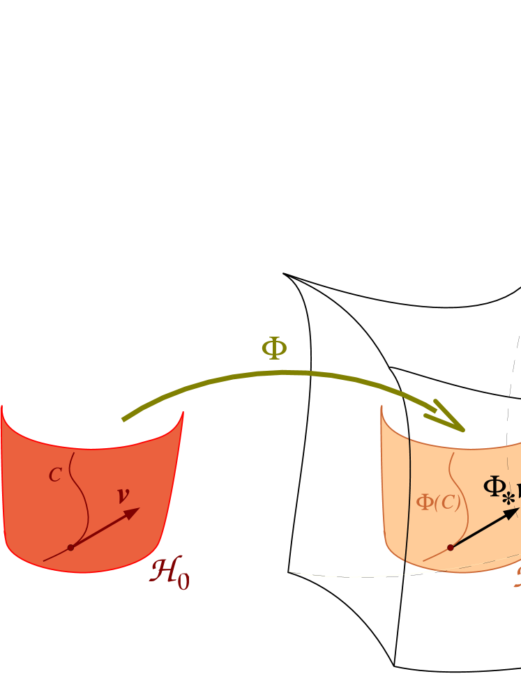
Figure 2.1: Embedding $\Phi$ of the 3-dimensional manifold ${\mathcal{H}}_{0}$ into the 4-dimensional manifold ${\mathcal{M}}$, defining the hypersurface ${\mathcal{H}}=\Phi({\mathcal{H}}_{0})$. The push-forward $\Phi_{*}\bm{v}$ of a vector $\bm{v}$ tangent to some curve $C$ in ${\mathcal{H}}_{0}$ is a vector tangent to $\Phi(C)$ in ${\mathcal{M}}$.

2.1 Definition of a hypersurface

A hypersurface ${\mathcal{H}}$ of ${\mathcal{M}}$ is the image of a 3-dimensional manifold ${\mathcal{H}}_{0}$ by an embedding $\Phi\,:\,{\mathcal{H}}_{0}\rightarrow{\mathcal{M}}$ (Fig. 2.1) :

$${\mathcal{H}}=\Phi({\mathcal{H}}_{0}).$$ (2.1)

Let us recall that embedding means that $\Phi\,:\,{\mathcal{H}}_{0}\rightarrow{\mathcal{H}}$ is a homeomorphism, i.e. a one-to-one mapping such that both $\Phi$ and $\Phi^{-1}$ are continuous. The one-to-one character guarantees that ${\mathcal{H}}$ does not “intersect itself”. A hypersurface can be defined locally as the set of points for which a scalar field on ${\mathcal{M}}$, $u$ let say, is constant:

$$\forall p\in{\mathcal{M}},\quad p\in{\mathcal{H}}\iff u(p)=1.$$ (2.2)

For instance, let us assume that ${\mathcal{H}}$ is a connected submanifold of ${\mathcal{M}}$ with topology $\mathbb{R}\times\mathbb{S}^{2}$. Then we may introduce locally a coordinate system of ${\mathcal{M}}$, $x^{\alpha}=(t,u,\theta,\varphi)$, such that $t$ spans $\mathbb{R}$ and $(\theta,\varphi)$ are spherical coordinates spanning $\mathbb{S}^{2}$. ${\mathcal{H}}$ is then defined by the coordinate condition $u=1$ [Eq. (2.2)] and an explicit form of the mapping $\Phi$ can be obtained by considering $x^{A}=(t,\theta,\varphi)$ as coordinates on the 3-manifold ${\mathcal{H}}_{0}$ :

$$\begin{array}[]{cccc}\Phi\ :&{\mathcal{H}}_{0}&\longrightarrow&{\mathcal{M}}\\ &(t,\theta,\varphi)&\longmapsto&(t,1,\theta,\varphi).\end{array}$$ (2.3)

In what follows, we identify ${\mathcal{H}}_{0}$ and ${\mathcal{H}}=\Phi({\mathcal{H}}_{0})$ (consequently, $\Phi$ can be seen as the inclusion map $\Phi:{\mathcal{H}}\longrightarrow{\mathcal{M}}$).

The embedding $\Phi$ “carries along” curves in ${\mathcal{H}}$ to curves in ${\mathcal{M}}$. Consequently it also “carries along” vectors on ${\mathcal{H}}$ to vectors on ${\mathcal{M}}$ (cf. Fig. 2.1). In other words, it defines a push-forward mapping $\Phi_{*}$ between ${\mathcal{T}}_{p}({\mathcal{H}})$ and ${\mathcal{T}}_{p}({\mathcal{M}})$. Thanks to the adapted coordinate systems $x^{\alpha}=(t,u,\theta,\varphi)$, the push-forward mapping can be explicited as follows

$$\begin{array}[]{cccc}\Phi_{*}\ :&{\mathcal{T}}_{p}({\mathcal{H}})&\longrightarrow&{\mathcal{T}}_{p}({\mathcal{M}})\\ &\bm{v}=(v^{t},v^{\theta},v^{\varphi})&\longmapsto&\Phi_{*}\bm{v}=(v^{t},0,v^{\theta},v^{\varphi}),\end{array}$$ (2.4)

where $v^{A}=(v^{t},v^{\theta},v^{\varphi})$ denotes the components of the vector $\bm{v}$ with respect to the natural basis $\partial/\partial x^{A}$ of ${\mathcal{T}}_{p}({\mathcal{H}})$ associated with the coordinates $(x^{A})$.

Conversely, the embedding $\Phi$ induces a pull-back mapping $\Phi^{*}$ between the linear forms on ${\mathcal{T}}_{p}({\mathcal{M}})$ and those on ${\mathcal{T}}_{p}({\mathcal{H}})$ as follows

$$\begin{array}[]{ccccccc}\Phi^{*}\ :&{\mathcal{T}}_{p}^{*}({\mathcal{M}})&\longrightarrow&{\mathcal{T}}_{p}^{*}({\mathcal{H}})&&&\\ &\bm{\omega}&\longmapsto&\Phi^{*}\bm{\omega}\ :&{\mathcal{T}}_{p}({\mathcal{H}})&\rightarrow&\mathbb{R}\\ &&&&\bm{v}&\mapsto&\langle\bm{\omega},\Phi_{*}\bm{v}\rangle.\end{array}$$ (2.5)

Taking into account (2.4), the pull-back mapping can be explicited:

$$\begin{array}[]{cccc}\Phi^{*}\ :&{\mathcal{T}}_{p}^{*}({\mathcal{M}})&\longrightarrow&{\mathcal{T}}_{p}^{*}({\mathcal{H}})\\ &\bm{\omega}=(\omega_{t},\omega_{u},\omega_{\theta},\omega_{\varphi})&\longmapsto&\Phi^{*}\bm{\omega}=(\omega_{t},\omega_{\theta},\omega_{\varphi}),\end{array}$$ (2.6)

where $\omega_{\alpha}$ denotes the components of the 1-form $\bm{\omega}$ with respect to the basis $\bm{\mathrm{d}}x^{\alpha}$ associated with the coordinates $(x^{\alpha})$. The pull-back operation can be extended to the multi-linear forms on ${\mathcal{T}}_{p}({\mathcal{M}})$ in an obvious way: if $\bm{T}$ is a $n$-linear form on ${\mathcal{T}}_{p}({\mathcal{M}})$, $\Phi^{*}\bm{T}$ is the $n$-linear form on ${\mathcal{T}}_{p}({\mathcal{H}})$ defined by

$$\forall(\bm{v}_{1},\ldots,\bm{v}_{n})\in{\mathcal{T}}_{p}({\mathcal{H}})^{n},\quad\Phi^{*}\bm{T}(\bm{v}_{1},\ldots,\bm{v}_{n})=\bm{T}(\Phi_{*}\bm{v}_{1},\ldots,\Phi_{*}\bm{v}_{n}).$$ (2.7)

Remark 2.1

By itself, the embedding $\Phi$ induces a mapping from vectors on ${\mathcal{H}}$ to vectors on ${\mathcal{M}}$ (push-forward mapping $\Phi_{*}$) and a mapping from 1-forms on ${\mathcal{M}}$ to 1-forms on ${\mathcal{H}}$ (pull-back mapping $\Phi^{*}$), but not in the reverse way. For instance, one may define “naively” a reverse mapping $F:\;{\mathcal{T}}_{p}({\mathcal{M}})\longrightarrow{\mathcal{T}}_{p}({\mathcal{H}})$ by $\bm{v}=(v^{t},v^{u},v^{\theta},v^{\varphi})\longmapsto F\bm{v}=(v^{t},v^{\theta},v^{\varphi})$, but it would then depend on the choice of coordinates $(t,u,\theta,\varphi)$, which is not the case of the push-forward mapping defined by Eq. (2.4). For spacelike or timelike hypersurfaces, the reverse mapping is unambiguously provided by the orthogonal projector (with respect to the ambient metric $\bm{g}$) onto the hypersurface. In the case of a null hypersurface, there is no such a thing as an orthogonal projector, as we shall see below (Remark 2.3).

A very important case of pull-back operation is that of the bilinear form $\bm{g}$ (i.e. the spacetime metric), which defines the induced metric on ${\mathcal{H}}$ :

$$\framebox{$\displaystyle\bm{q}:=\Phi^{*}\bm{g}$}$$ (2.8)

$\bm{q}$ is also called the first fundamental form of ${\mathcal{H}}$. In terms of the coordinate system $x^{A}=(t,\theta,\varphi)$ of ${\mathcal{H}}$, the components of $\bm{q}$ are deduced from (2.6):

$$q_{AB}=g_{AB}.$$ (2.9)

2.2 Definition of a null hypersurface

The hypersurface ${\mathcal{H}}$ is said to be null (or lightlike, or characteristic or to be a wavefront) if, and only if, the induced metric $\bm{q}$ is degenerate. This means if, and only if, there exists a non-vanishing vector field $\bm{\ell}$ in ${\mathcal{T}}({\mathcal{H}})$ which is orthogonal (with respect to $\bm{q}$) to all vector fields in ${\mathcal{T}}({\mathcal{H}})$:

$$\forall\bm{v}\in{\mathcal{T}}({\mathcal{H}}),\quad\bm{q}(\bm{\ell},\bm{v})=0.$$ (2.10)

The signature of $\bm{q}$ is then necessarily $(0,+,+)$. An equivalent definition of a null hypersurface demands any vector field $\bm{\ell}$ in ${\mathcal{T}}({\mathcal{M}})$ which is normal to ${\mathcal{H}}$ [i.e. orthogonal to all vectors in ${\mathcal{T}}({\mathcal{H}})$] to be a null vector with respect to the metric $\bm{g}$:

$$\framebox{$\displaystyle\bm{g}(\bm{\ell},\bm{\ell})=\bm{\ell}\cdot\bm{\ell}=0$}.$$ (2.11)

We adopt the same notation $\bm{\ell}$ than in the previous definition, since this $\bm{\ell}$ is nothing but the pushed-forward by $\Phi_{*}$ of the $\bm{\ell}$ in ${\mathcal{T}}({\mathcal{H}})$. Indeed, by saying that $\bm{\ell}$ is orthogonal to itself, Eq. (2.11) states that $\bm{\ell}$ is tangent to ${\mathcal{H}}$. A distinctive property of null hypersurfaces is that their normal vectors are both orthogonal and tangent to them.

Since the hypersurface ${\mathcal{H}}$ is defined by a constant value of the scalar field $u$ [Eq. (2.2)], the gradient 1-form $\bm{\mathrm{d}}u$ is normal to ${\mathcal{H}}$, i.e.

$$\forall\bm{v}\in{\mathcal{T}}({\mathcal{M}}),\quad\bm{v}\in{\mathcal{T}}({\mathcal{H}})\iff\langle\bm{\mathrm{d}}u,\bm{v}\rangle=0.$$ (2.12)

As a side remark notice that, in terms of the components $v^{\alpha}$ of $\bm{v}$ with respect to the natural basis associated with the coordinates $(x^{\alpha})$, $\langle\bm{\mathrm{d}}u,\bm{v}\rangle=v^{u}$ and the above property is equivalent to

$$\forall\bm{v}\in{\mathcal{T}}({\mathcal{M}}),\quad\bm{v}\in{\mathcal{T}}({\mathcal{H}})\iff v^{u}=0,$$ (2.13)

which agrees with (2.4). From (2.12), it is obvious that the 1-form $\underline{\bm{\ell}}$ associated with the normal vector $\bm{\ell}$ by the standard metric duality [cf. notation (1.10)] must be collinear to $\bm{\mathrm{d}}u$:

$$\framebox{$\displaystyle\underline{\bm{\ell}}=\e^{\rho}\bm{\mathrm{d}}u$},$$ (2.14)

where $\rho$ is some scalar field on ${\mathcal{H}}$. We have chosen the coefficient relating $\underline{\bm{\ell}}$ and $\bm{\mathrm{d}}u$ to be strictly positive, i.e. under the form of an exponential. This is always possible by a suitable choice of the scalar field $u$.

The characterization of ${\mathcal{T}}_{p}({\mathcal{H}})$ as a hyperplane of the vector space ${\mathcal{T}}_{p}({\mathcal{M}})$ can then be expressed as follows:

$$\framebox{$\displaystyle\forall\bm{v}\in{\mathcal{T}}_{p}({\mathcal{M}}),\quad\bm{v}\in{\mathcal{T}}_{p}({\mathcal{H}})\iff\langle\underline{\bm{\ell}},\bm{v}\rangle=\bm{\ell}\cdot\bm{v}=0$}.$$ (2.15)

Remark 2.2

Since the scalar square of $\bm{\ell}$ is zero [Eq. (2.11)], there is no natural normalization of $\bm{\ell}$, contrary to the case of spacelike hypersurfaces, where one can always choose the normal to be a unit vector (scalar square equal to $-1$). Equivalently, there is no natural choice of the factor $\rho$ in relation (2.14). In Sec. 4, we will use the extra-structure introduced in ${\mathcal{M}}$ by the spacelike foliation of the 3+1 formalism to set unambiguously the normalization of $\bm{\ell}$.

Remark 2.3

Another distinctive feature of null hypersurfaces, with respect to spacelike or timelike ones, is the absence of orthogonal projector onto them. This is a direct consequence of the fact that the normal $\bm{\ell}$ is tangent to ${\mathcal{H}}$. Indeed, suppose we define “naively” $\bm{\Pi}:=\bm{1}+a\bm{\ell}\langle\underline{\bm{\ell}},.\rangle$ (or in index notation : $\Pi^{\alpha}_{\ \beta}:=\delta^{\alpha}_{\ \beta}+a\ell^{\alpha}\ell_{\beta}$) as the “orthogonal projector” with some coefficient $a$ to be determined ($a=1$ for a spacelike hypersurface and $a=-1$ for a timelike hypersurface, if $\bm{\ell}$ is the unit normal). Then it is true that for any $\bm{v}\in{\mathcal{T}}_{p}({\mathcal{H}})$, $\bm{\Pi}(\bm{v})=\bm{v}$, but if $\bm{v}\not\in{\mathcal{T}}_{p}({\mathcal{H}})$, $\bm{\ell}\cdot\bm{\Pi}(\bm{v})=\bm{\ell}\cdot\bm{v}\not=0$, which shows that $\bm{\Pi}(\bm{v})\not\in{\mathcal{T}}_{p}({\mathcal{H}})$, hence the endomorphism $\bm{\Pi}$ is not a projector on ${\mathcal{T}}_{p}({\mathcal{H}})$, whatever the value of $a$. This lack of orthogonal projector implies that there is no canonical way, from the null structure alone, to define a mapping ${\mathcal{T}}_{p}({\mathcal{M}})\longrightarrow{\mathcal{T}}_{p}({\mathcal{H}})$ (cf. Remark 2.1).

2.3 Auxiliary null foliation in the vicinity of ${\mathcal{H}}$

The null normal vector field $\bm{\ell}$ is a priori defined on ${\mathcal{H}}$ only and not at points $p\not\in{\mathcal{H}}$. However within the 4-dimensional point of view adopted in this article, we would like to consider $\bm{\ell}$ as a vector field not confined to ${\mathcal{H}}$ but defined in some open subset of ${\mathcal{M}}$ around ${\mathcal{H}}$. In particular this would permit to define the spacetime covariant derivative $\bm{\nabla}\bm{\ell}$, which is not possible if the support of $\bm{\ell}$ is restricted to ${\mathcal{H}}$. Following Carter [43], a simple way to achieve this is to consider not only a single null hypersurface ${\mathcal{H}}$, but a foliation of ${\mathcal{M}}$ (in the vicinity of ${\mathcal{H}}$) by a family of null hypersurfaces, such that ${\mathcal{H}}$ is an element of this family. Without any loss of generality, we may select the scalar field $u$ to label these hypersurfaces and denote the family by $({\mathcal{H}}_{u})$. The null hypersurface ${\mathcal{H}}$ is then nothing but the element ${\mathcal{H}}={\mathcal{H}}_{u=1}$ of this family [Eq. (2.2)]. The vector field $\bm{\ell}$ can then be viewed as defined in the part of ${\mathcal{M}}$ foliated by $({\mathcal{H}}_{u})$, such that at each point in this region, $\bm{\ell}$ is null and normal to ${\mathcal{H}}_{u}$ for some value of $u$. The identity (2.14) is then valid for this “extended” $\bm{\ell}$, and $\rho$ is now a scalar field defined not only on ${\mathcal{H}}$ but in the open region of ${\mathcal{M}}$ around ${\mathcal{H}}$ which is foliated by $({\mathcal{H}}_{u})$.

Obviously the family $({\mathcal{H}}_{u})$ is non-unique but all geometrical quantities that we shall introduce hereafter do not depend upon the choice of the foliation ${\mathcal{H}}_{u}$ once they are evaluated at ${\mathcal{H}}$.

2.4 Frobenius identity

The identity (2.14) which expresses that the 1-form $\underline{\bm{\ell}}$ is normal to a hypersurface $u={\rm const}$, leads to a particular form for the exterior derivative of $\underline{\bm{\ell}}$. Indeed, taking the exterior derivative of (2.14) (considering $\underline{\bm{\ell}}$ defined in a open neighborhood of ${\mathcal{H}}$ in ${\mathcal{M}}$, cf. Sec. 2.3) and applying rule (1.22) (with $\e^{\rho}$ = 0-form) leads to

$$\bm{\mathrm{d}}\underline{\bm{\ell}}=\e^{\rho}\bm{\mathrm{d}}\rho\wedge\bm{\mathrm{d}}u+\e^{\rho}\bm{\mathrm{d}}\bm{\mathrm{d}}u.$$ (2.16)

Since $\bm{\mathrm{d}}\bm{\mathrm{d}}=0$ is a basic property of the exterior derivative, the last term on the right-hand side of (2.16) vanishes [this is also obvious by applying Eq. (1.23) to the 1-form $\bm{\mathrm{d}}u$]. Hence, after replacing $\bm{\mathrm{d}}u$ by $\e^{-\rho}\underline{\bm{\ell}}$, one is left with

$$\framebox{$\displaystyle\bm{\mathrm{d}}\underline{\bm{\ell}}=\bm{\mathrm{d}}\rho\,\wedge\underline{\bm{\ell}}$}.$$ (2.17)

This reflects the Frobenius theorem in its dual formulation (see e.g. Theorem B.3.2 in Wald’s textbook [167]): the exterior derivative of the 1-form $\underline{\bm{\ell}}$ is the exterior product of $\underline{\bm{\ell}}$ itself with some 1-form ($\bm{\mathrm{d}}\rho$ in the present case) if, and only if, $\underline{\bm{\ell}}$ defines hyperplanes of ${\mathcal{T}}({\mathcal{M}})$ [by Eq. (2.15)] which are integrable in some hypersurface (${\mathcal{H}}$ in the present case).

2.5 Generators of ${\mathcal{H}}$ and non-affinity coefficient $\kappa$

Let us establish a fundamental property of null hypersurfaces: they are ruled by null geodesics. Contracting Eq. (2.17) with $\bm{\ell}$ and using the fact that $\bm{\ell}$ is null, gives

$$\bm{\ell}\cdot\bm{\mathrm{d}}\underline{\bm{\ell}}=\langle\bm{\mathrm{d}}\rho,\bm{\ell}\rangle\,\underline{\bm{\ell}}-\underbrace{\langle\underline{\bm{\ell}},\bm{\ell}\rangle}_{=0}\bm{\mathrm{d}}\rho=\langle\bm{\mathrm{d}}\rho,\bm{\ell}\rangle\,\underline{\bm{\ell}}.$$ (2.18)

On the other side if we express the exterior derivative $\bm{\mathrm{d}}\underline{\bm{\ell}}$ in terms of the covariant derivative $\bm{\nabla}$ associated with the spacetime metric $\bm{g}$, the left-hand side of the above equation becomes

$$(\bm{\ell}\cdot\bm{\mathrm{d}}\underline{\bm{\ell}})_{\alpha}=\ell^{\mu}\nabla_{\mu}\ell_{\alpha}-\ell^{\mu}\nabla_{\alpha}\ell_{\mu}=\ell^{\mu}\nabla_{\mu}\ell_{\alpha}=(\bm{\nabla}_{\bm{\ell}}\,\underline{\bm{\ell}})_{\alpha},$$ (2.19)

where we have used $\ell^{\mu}\nabla_{\alpha}\ell_{\mu}=1/2\;\nabla_{\alpha}(\ell^{\mu}\ell_{\mu})=0$. Hence Eq. (2.18) leads to

$$\bm{\nabla}_{\bm{\ell}}\,\underline{\bm{\ell}}=\langle\bm{\mathrm{d}}\rho,\bm{\ell}\rangle\,\underline{\bm{\ell}},$$ (2.20)

or by the metric duality between 1-forms and vectors:

$$\framebox{$\displaystyle\bm{\nabla}_{\bm{\ell}}\,\bm{\ell}=\kappa\,\bm{\ell}$},$$ (2.21)

where $\kappa$ is the scalar field defined on ${\mathcal{H}}$ by

$$\framebox{$\displaystyle\kappa:=\bm{\nabla}_{\bm{\ell}}\,\rho=\langle\bm{\mathrm{d}}\rho,\bm{\ell}\rangle$}.$$ (2.22)

In the case where ${\mathcal{H}}$ is the horizon of a Kerr black hole, $\bm{\ell}$ can be normalized to become a Killing vector of $({\mathcal{M}},\bm{g})$, of the form $\bm{\ell}=\bm{\xi}_{0}+\Omega_{{\mathcal{H}}}\bm{\xi}_{1}$, where $\Omega_{{\mathcal{H}}}={\rm const}$ and $\bm{\xi}_{0}$ and $\bm{\xi}_{1}$ are the Killing vectors associated with respectively the stationarity and axisymmetry of Kerr spacetime and normalized so that the parameter length of $\bm{\xi}_{1}$’s orbits is $2\pi$ and $\bm{\xi}_{0}$ asymptotically coincides with the 4-velocity of an inertial observer. $\kappa$ is then called the surface gravity of the black hole (see Appendix D for further details).

Since Eq. (2.21) involves only the derivative of $\bm{\ell}$ along $\bm{\ell}$, i.e. within ${\mathcal{H}}$, the definition of $\kappa$ is intrinsic to $({\mathcal{H}},\bm{\ell})$ and does not depend upon the choice of the auxiliary null foliation $({\mathcal{H}}_{u})$.

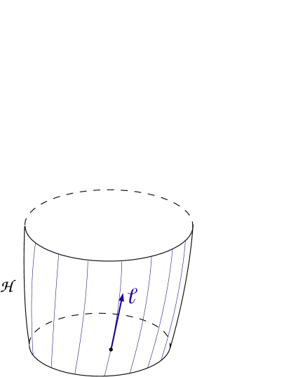
Figure 2.2: Null hypersurface ${\mathcal{H}}$ with some null normal $\bm{\ell}$ and the null generators (thin lines).

Equation (2.21) means that $\bm{\ell}$ remains colinear to itself when it is parallely transported along its field lines. This implies that these field lines are spacetime geodesics. Indeed, by a suitable choice of the renormalization factor $\alpha$ such that $\bm{\ell}^{\prime}=\alpha\bm{\ell}$, Eq. (2.21) can be brought to the classical “equation of geodesics” form:

$$\bm{\nabla}_{\bm{\ell}^{\prime}}\,\bm{\ell}^{\prime}=0.$$ (2.23)

This is immediate since

$$\bm{\nabla}_{\bm{\ell}^{\prime}}\,\bm{\ell}^{\prime}=\alpha\left[\alpha\bm{\nabla}_{\bm{\ell}}\,\bm{\ell}+\left(\bm{\nabla}_{\bm{\ell}}\,\alpha\right)\bm{\ell}\right]=\alpha^{2}\left(\kappa+\bm{\nabla}_{\bm{\ell}}\,\ln\alpha\right)\bm{\ell}$$ (2.24)

and one can choose $\alpha$ to get Eq. (2.23) by requiring it to be a solution of the following first order differential equation along the field lines of $\bm{\ell}$

$$\bm{\nabla}_{\bm{\ell}}\,\ln\alpha=-\kappa.$$ (2.25)

If $\kappa\not=0$, Eq. (2.21) means that the parameter $\tau$ associated with $\bm{\ell}$ by $\ell^{\alpha}=dx^{\alpha}/d\tau$ is not an affine parameter of the geodesics. For this reason, we may call $\kappa$ the non-affinity coefficient. Note that (2.24) gives the following scaling law for $\kappa$:

$$\bm{\ell}\rightarrow\bm{\ell}^{\prime}=\alpha\bm{\ell}\quad\Longrightarrow\quad\kappa\rightarrow\kappa^{\prime}=\alpha\left(\kappa+\bm{\nabla}_{\bm{\ell}}\,\ln\alpha\right).$$ (2.26)

Having established that the field lines of $\bm{\ell}$ are geodesics, it is obvious that they are null geodesics (for $\bm{\ell}$ is null). They are called the null generators of ${\mathcal{H}}$. Note that whereas $\bm{\ell}$ is not uniquely defined, being subject to the rescaling law $\bm{\ell}\rightarrow\bm{\ell}^{\prime}=\alpha\bm{\ell}$, the null generators, considered as 1-dimensional curves in ${\mathcal{M}}$, are unique (see Fig. 2.2). In other words, they depend only upon ${\mathcal{H}}$.

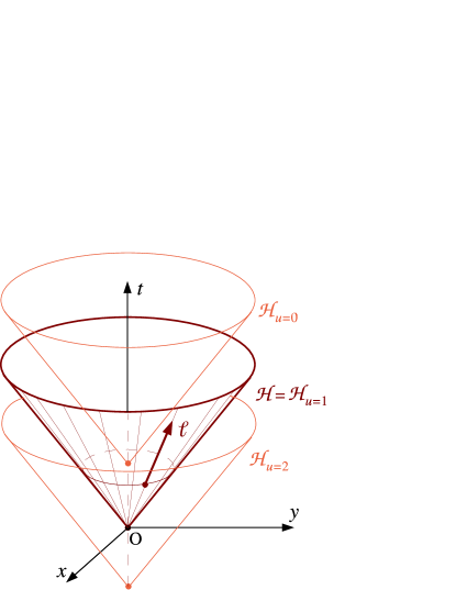
Figure 2.3: Outgoing light cone in Minkowski spacetime. The null hypersurface ${\mathcal{H}}$ under consideration is the member $u=1$ of the family $({\mathcal{H}}_{u})$ of light cones emitted from the origin $(x,y,z)=(0,0,0)$ at successive times $t=1-u$.

Example 2.4

Outgoing light cone in Minkowski spacetime.
The simplest example of a null hypersurface one may think of is the light cone in Minkowski spacetime (Fig. 2.3). More precisely, let us consider for ${\mathcal{H}}$ the outgoing light cone from a given point $O$, excluding $O$ itself to keep ${\mathcal{H}}$ smooth. If $(x^{\alpha})=(t,x,y,z)$ denote standard Minkowskian coordinates with origin $O$, the scalar field $u$ defining ${\mathcal{H}}$ as the level set $u=1$ is then

$$u(t,x,y,z):=r-t+1\quad\mbox{with}\quad r:=\sqrt{x^{2}+y^{2}+z^{2}}.$$ (2.27)

Note that $u$ generates not only ${\mathcal{H}}$, but a full null foliation $({\mathcal{H}}_{u})$ as the level sets of $u$ (cf. Sec. 2.3). The member ${\mathcal{H}}_{u}$ of this foliation is then nothing but the light cone emanating from the point $(-u+1,0,0,0)$ (cf. Fig. 2.3). In terms of components with respect to the coordinates $(x^{\alpha})$, the gradient 1-form $\bm{\mathrm{d}}u$ is $\nabla_{\alpha}u=(-1,x/r,y/r,z/r)$. Hence, from Eq. (2.14), the null normal to ${\mathcal{H}}$ is $\ell^{\alpha}=e^{\rho}(1,x/r,y/r,z/r)$. For simplicity, let us select $\rho=0$. Then

$$\ell^{\alpha}=\left(1,\frac{x}{r},\frac{y}{r},\frac{z}{r}\right)\qquad\mbox{and}\qquad\ell_{\alpha}=\left(-1,\frac{x}{r},\frac{y}{r},\frac{z}{r}\right).$$ (2.28)

The gradient bilinear form $\bm{\nabla}\underline{\bm{\ell}}$ is easily computed since, for the coordinates $(t,x,y,z)$, $\nabla_{\beta}\ell_{\alpha}=\partial\ell_{\alpha}/\partial x^{\beta}$:

$$\nabla_{\beta}\ell_{\alpha}=\left(\begin{array}[]{cccc}0&0&0&0\\ 0&\frac{y^{2}+z^{2}}{r^{3}}&-\frac{xy}{r^{3}}&-\frac{xz}{r^{3}}\\ 0&-\frac{xy}{r^{3}}&\frac{x^{2}+z^{2}}{r^{3}}&-\frac{yz}{r^{3}}\\ 0&-\frac{xz}{r^{3}}&-\frac{yz}{r^{3}}&\frac{x^{2}+y^{2}}{r^{3}}\end{array}\right)\qquad\begin{array}[]{ll}(&\mbox{\rm$\alpha$ = row index;}\\ &\mbox{\rm$\beta$ = column index).}\end{array}$$ (2.29)

We may check immediately on this formula that $\ell^{\mu}\nabla_{\mu}\ell_{\alpha}=0$, which leads to

$$\kappa=0,$$ (2.30)

in accordance with $\kappa=\bm{\nabla}_{\bm{\ell}}\,\rho$ [Eq. (2.22)] and our choice $\rho=0$. Actually it is easy to check that the coordinate $t$ is an affine parameter of the null geodesics generating ${\mathcal{H}}$ and that $\bm{\ell}$ is the associated tangent vector, hence the vanishing of the non-affinity coefficient $\kappa$.

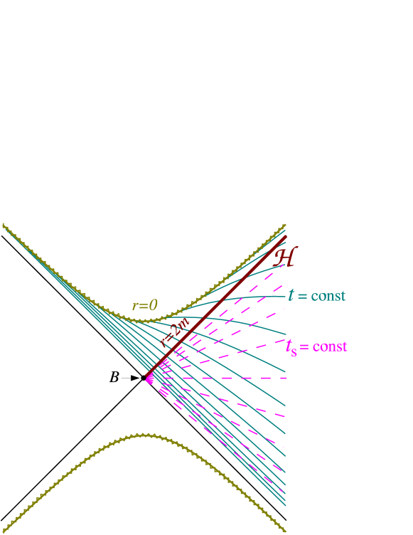
Figure 2.4: Kruskal diagram representing the Schwarzschild spacetime; the hypersurfaces of constant Schwarzschild time $t_{\rm S}$ (dashed lines) do not intersect the future event horizon ${\mathcal{H}}$, except at the bifurcation 2-sphere $B$ (reduced to a point in the figure), whereas the hypersurfaces of constant Eddington-Finkelstein time $t$ (solid lines) intersect it in such a way that $t$ can be used as a regular coordinate on ${\mathcal{H}}$ (figure adapted from Fig. 3.1 of Ref. [161]).

Example 2.5

Schwarzschild horizon in Eddington-Finkelstein coordinates.
The next example of null surface one might think about is the (future) event horizon of a Schwarzschild black hole. The corresponding spacetime is often (partially) described by two sets of coordinates: (i) the Schwarzschild coordinates $(t_{\rm S},r,\theta,\varphi)$, in which the metric components are given by

$$g_{\mu\nu}dx^{\mu}dx^{\nu} = -\left(1-\frac{2m}{r}\right)dt_{\rm S}^{2}+\left(1-\frac{2m}{r}\right)^{-1}dr^{2}+r^{2}(d\theta^{2}+\sin^{2}\theta d\varphi^{2}),$$

where $m$ is the mass of the black hole, and (ii) the isotropic coordinates $(t_{\rm S},\tilde{r},\theta,\varphi)$, resulting in the metric components

$$g_{\mu\nu}dx^{\mu}dx^{\nu} = -\left(\frac{1-\frac{m}{2\tilde{r}}}{1+\frac{m}{2\tilde{r}}}\right)^{2}dt_{\rm S}^{2}+\left(1+\frac{m}{2\tilde{r}}\right)^{4}\left[d{\tilde{r}}^{2}+{\tilde{r}}^{2}(d\theta^{2}+\sin^{2}\theta d\varphi^{2})\right].$$

The relation between the two sets of coordinates is given by $r={\tilde{r}}\left(1+\frac{m}{2\tilde{r}}\right)^{2}$. As it is well known, the above two coordinate systems are singular at the event horizon ${\mathcal{H}}$, which corresponds to $r=2m$, $\tilde{r}=m/2$ and $t_{\rm S}\rightarrow+\infty$. In particular the hypersurfaces of constant time $t_{\rm S}$, which constitutes a well known example of maximal slicing (cf. Sec. 3), do not intersect ${\mathcal{H}}$, except at a 2-sphere (named the bifurcation sphere), where they also cross each other (this is illustrated by the Kruskal diagram in Fig. 2.4).

A coordinate system, well known for being regular at ${\mathcal{H}}$, is constructed with the ingoing Eddington-Finkelstein coordinates $(V,r,\theta,\varphi)$, where the coordinate $V$ is constant on each ingoing radial null geodesic and is related to the Schwarzschild coordinate time $t_{\rm S}$ by $V=t_{\rm S}+r+2m\ln\left|\frac{r}{2m}-1\right|$. The coordinate $V$ is null, but if we introduce

$$t:=V-r=t_{\rm S}+2m\ln\left|\frac{r}{2m}-1\right|,$$ (2.33)

we get a timelike coordinate. The system $(t,r,\theta,\varphi)$ is called the 3+1 Eddington-Finkelstein coordinates. These coordinates are well behaved in the vicinity of ${\mathcal{H}}$, as shown in Fig. 2.4, and yields to the following metric components:

$$g_{\mu\nu}dx^{\mu}dx^{\nu} = -\left(1-\frac{2m}{r}\right)dt^{2}+\frac{4m}{r}\,dt\,dr+\left(1+\frac{2m}{r}\right)dr^{2}$$ (2.34)

$$+r^{2}(d\theta^{2}+\sin^{2}\theta d\varphi^{2}).$$

It is clear on this expression that the 3+1 Eddington-Finkelstein coordinates are regular at the event horizon ${\mathcal{H}}$, which is located at $r=2m$ (cf. Fig. 2.5). However, we cannot use $u=r-2m+1$ for the scalar field defining ${\mathcal{H}}$, because the hypersurfaces $r={\rm const}$ are not null, except for $r=2m$, whereas we have required in Sec. 2.3 all the hypersurfaces $u={\rm const}$ to be null. Actually, a family of null hypersurfaces encompassing ${\mathcal{H}}$ is given by the constant values of the outgoing Eddington-Finkelstein coordinate

$$U=t_{\rm S}-r-2m\ln\left|\frac{r}{2m}-1\right|=t-r-4m\ln\left|\frac{r}{2m}-1\right|.$$ (2.35)

The event horizon corresponds to $U=+\infty$; to get finite values, let us replace $U$ by the null Kruskal-Szekeres coordinate (shifted by 1)

$$u:=\pm\exp\left(-\frac{U}{4m}\right)+1,$$ (2.36)

where the $+$ sign (resp. $-$ sign) is for $r\geq 2m$ (resp. $r<2m$). Then

$$u=\left(\frac{r}{2m}-1\right)\exp\left(\frac{r-t}{4m}\right)+1$$ (2.37)

and all the hypersurfaces ${\mathcal{H}}_{u}$ defined by $u={\rm const}$ are null (there are drawn in Fig. 2.5), the event horizon ${\mathcal{H}}$ corresponding to $u=1$.

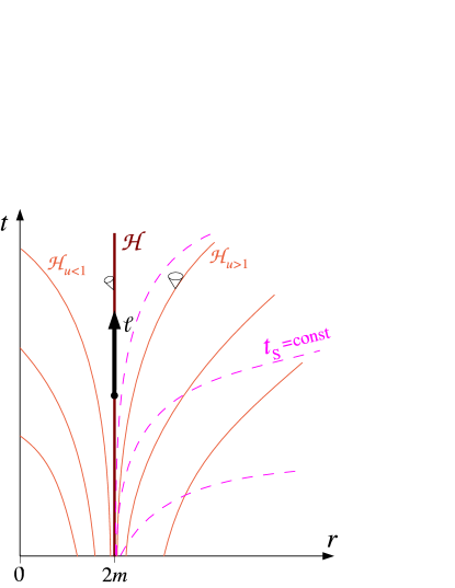
Figure 2.5: Event horizon ${\mathcal{H}}$ of a Schwarzschild black hole in 3+1 Eddington-Finkelstein coordinates. The dashed lines represents the hypersurfaces of constant Schwarzschild time $t_{\rm S}$ shown in Fig. 2.4.

The null normals to ${\mathcal{H}}_{u}$ are deduced from the gradient of $u$ by $\ell_{\alpha}=\e^{\rho}\nabla_{\alpha}u$ [Eq. (2.14)]. We get the following components with respect to the 3+1 Eddington-Finkelstein coordinates $(x^{\alpha})=(t,r,\theta,\varphi)$:

$$\ell^{\alpha}=\frac{1}{4m}\exp\left(\rho+\frac{r-t}{4m}\right)\,\left(1+\frac{r}{2m},\ \frac{r}{2m}-1,\ 0,\ 0\right).$$ (2.38)

Let us choose $\rho$ such that $\ell^{t}=1$. Then

$$\rho=\frac{t-r}{4m}-\ln\left(1+\frac{r}{2m}\right)+\ln(4m),$$ (2.39)

$$\ell^{\alpha}=\left(1,\frac{r-2m}{r+2m},0,0\right)\qquad\mbox{and}\qquad\ell_{\alpha}=\left(\frac{2m-r}{r+2m},1,0,0\right).$$ (2.40)

Note that on the horizon, $\ell^{\alpha}\stackrel{{\scriptstyle{\mathcal{H}}}}{{=}}(1,0,0,0)$, i.e.

$$\bm{\ell}\stackrel{{\scriptstyle{\mathcal{H}}}}{{=}}\bm{t},$$ (2.41)

where $\bm{t}=\partial/\partial t$ is a Killing vector associated with the stationarity of Schwarzschild solution. The gradient of $\bm{\ell}$ is obtained by a straightforward computation, after having evaluated the connection coefficients from the metric components given by Eq. (2.34):

$$\nabla_{\beta}\ell_{\alpha} = \left(\begin{array}[]{cccc}\frac{m}{r^{2}}\frac{2m-r}{r+2m}&\frac{m(3m^{2}+4mr-3r^{2})}{r^{2}(r+2m)^{2}}&0&0\\ \frac{m}{r^{2}}&\frac{m(3r+2m)}{r^{2}(r+2m)}&0&0\\ 0&0&\frac{r(r-2m)}{r+2m}&0\\ 0&0&0&\frac{(r-2m)r\sin^{2}\theta}{r+2m}\end{array}\right)$$

$$\mbox{\rm($\alpha$ = row index;}\qquad\mbox{\rm$\beta$ = column index)}.$$

We deduce from these values that

$$\ell^{\mu}\nabla_{\mu}\ell_{\alpha}=\left(\frac{4m}{(r+2m)^{2}},\frac{4m(r-2m)}{(r+2m)^{3}},0,0\right).$$ (2.47)

Comparing with the expression (2.40) for $\ell_{\alpha}$, we deduce the value of the non-affinity coefficient [cf. Eq. (2.21)]:

$$\kappa=\frac{4m}{(r+2m)^{2}}.$$ (2.48)

As a check, we can recover $\kappa$ by means of formula (2.22), evaluating $\bm{\nabla}_{\bm{\ell}}\rho$ from expression (2.39) for $\rho$. Note that on the horizon,

$$\kappa\stackrel{{\scriptstyle{\mathcal{H}}}}{{=}}\frac{1}{4m},$$ (2.49)

which is the standard value for the surface gravity of a Schwarzschild black hole.

2.6 Weingarten map

As for any hypersurface, the “bending” of ${\mathcal{H}}$ in ${\mathcal{M}}$ (also called extrinsic curvature of ${\mathcal{H}}$) is described by the Weingarten map (sometimes called the shape operator), which is the endomorphism of ${\mathcal{T}}_{p}({\mathcal{H}})$ which associates with each vector tangent to ${\mathcal{H}}$ the variation of the normal along that vector, with respect to the spacetime connection $\bm{\nabla}$:

$$\framebox{$\displaystyle\begin{array}[]{cccc}\bm{\chi}:&{\mathcal{T}}_{p}({\mathcal{H}})&\longrightarrow&{\mathcal{T}}_{p}({\mathcal{H}})\\ &\bm{v}&\longmapsto&\bm{\nabla}_{\bm{v}}\,\bm{\ell}\end{array}$}$$ (2.50)

This application is well defined (i.e. its image is in ${\mathcal{T}}_{p}({\mathcal{H}})$) since

$$\bm{\ell}\cdot\bm{\chi}(\bm{v})=\bm{\ell}\cdot\bm{\nabla}_{\bm{v}}\,\bm{\ell}={1\over 2}\bm{\nabla}_{\bm{v}}(\bm{\ell}\cdot\bm{\ell})=0,$$ (2.51)

which shows that $\bm{\chi}(\bm{v})\in{\mathcal{T}}_{p}({\mathcal{H}})$ [cf. Eq. (2.15)]. Moreover, since it involves only the derivative of $\bm{\ell}$ along vectors tangent to ${\mathcal{H}}$, the definition of $\bm{\chi}$ is clearly independent of the choice of the auxiliary null foliation $({\mathcal{H}}_{u})$ introduced in Sec. 2.3.

Remark 2.6

The Weingarten map depends on the specific choice of the normal $\bm{\ell}$, in contrast with the timelike or spacelike case, where the unit length of the normal fixes it unambiguously. Indeed a rescaling of $\bm{\ell}$ acts as follows on $\bm{\chi}$:

$$\bm{\ell}\rightarrow\bm{\ell}^{\prime}=\alpha\bm{\ell}\quad\Longrightarrow\quad\bm{\chi}\rightarrow\bm{\chi}^{\prime}=\alpha\bm{\chi}+\langle\bm{\mathrm{d}}\alpha,\cdot\rangle\,\bm{\ell},$$ (2.52)

where the notation $\langle\bm{\mathrm{d}}\alpha,\cdot\rangle\,\bm{\ell}$ stands for the endomorphism ${\mathcal{T}}_{p}({\mathcal{H}})\longrightarrow{\mathcal{T}}_{p}({\mathcal{H}})$, $\bm{v}\longmapsto\langle\bm{\mathrm{d}}\alpha,\bm{v}\rangle\,\bm{\ell}$.

The fundamental property of the Weingarten map is to be self-adjoint with respect to the metric $\bm{q}$ [i.e. the pull-back of $\bm{g}$ on ${\mathcal{T}}({\mathcal{H}})$, cf. Eq. (2.8)]:

$$\framebox{$\displaystyle\forall(\bm{u},\bm{v})\in{\mathcal{T}}({\mathcal{H}})\times{\mathcal{T}}({\mathcal{H}}),\quad\bm{u}\cdot\bm{\chi}(\bm{v})=\bm{\chi}(\bm{u})\cdot\bm{v}$},$$ (2.53)

where the dot means the scalar product with respect to $\bm{q}$ [considering $\bm{u}$ and $\bm{v}$ as vectors of ${\mathcal{T}}({\mathcal{H}})$] or $\bm{g}$ [considering $\bm{u}$ and $\bm{v}$ as vectors of ${\mathcal{T}}({\mathcal{M}})$]. Indeed, one obtains from the definition of $\bm{\chi}$

$$\bm{u}\cdot\bm{\chi}(\bm{v}) = \bm{u}\cdot\bm{\nabla}_{\bm{v}}\,\bm{\ell}=\bm{\nabla}_{\bm{v}}\,(\bm{u}\cdot\bm{\ell})-\bm{\ell}\cdot\bm{\nabla}_{\bm{v}}\,\bm{u}=0-\bm{\ell}\cdot\left(\bm{\nabla}_{\bm{u}}\,\bm{v}-[\bm{u},\bm{v}]\right)$$ (2.54)

$$= -\bm{\nabla}_{\bm{u}}\,(\bm{\ell}\cdot\bm{v})+\bm{v}\cdot\bm{\nabla}_{\bm{u}}\,\bm{\ell}+\bm{\ell}\cdot[\bm{u},\bm{v}]$$

$$= 0+\bm{v}\cdot\bm{\chi}(\bm{u})+\bm{\ell}\cdot[\bm{u},\bm{v}],$$

where use has been made of $\bm{\ell}\cdot\bm{u}=0$ and $\bm{\ell}\cdot\bm{v}=0$. Now the Frobenius theorem states that the commutator $[\bm{u},\bm{v}]$ of two vectors of the hyperplane ${\mathcal{T}}({\mathcal{H}})$ belongs to ${\mathcal{T}}({\mathcal{H}})$ since ${\mathcal{T}}({\mathcal{H}})$ is surface-forming (see e.g. Theorem B.3.1 in Wald’s textbook [167]). It is straightforward to establish it:

$$\bm{\ell}\cdot[\bm{u},\bm{v}] = \langle\underline{\bm{\ell}},[\bm{u},\bm{v}]\rangle=\ell_{\mu}u^{\nu}\nabla_{\nu}v^{\mu}-\ell_{\mu}v^{\nu}\nabla_{\nu}u^{\mu}=-u^{\nu}v^{\mu}\nabla_{\nu}\ell_{\mu}+v^{\nu}u^{\mu}\nabla_{\nu}\ell_{\mu}$$

$$= (\nabla_{\mu}\ell_{\nu}-\nabla_{\nu}\ell_{\mu})u^{\nu}v^{\mu}=({\rm d}\underline{\ell})_{\mu\nu}\,u^{\nu}v^{\mu}=(\nabla_{\mu}\rho\;\ell_{\nu}-\nabla_{\nu}\rho\;\ell_{\mu})u^{\nu}v^{\mu}$$

$$\bm{\ell}\cdot[\bm{u},\bm{v}] = 0,$$ (2.55)

where use has been made of expression (2.17) for the exterior derivative of $\underline{\bm{\ell}}$ and the last equality results from $\ell_{\nu}u^{\nu}=0$ and $\ell_{\mu}v^{\mu}=0$. Inserting (2.55) into (2.54) establishes the self-adjointness of the Weingarten map.

Let us note that the non-affinity coefficient $\kappa$ is an eigenvalue of the Weingarten map, corresponding to the eigenvector $\bm{\bm{\ell}}$, since Eq. (2.21) can be written

$$\framebox{$\displaystyle\bm{\chi}(\bm{\ell})=\kappa\bm{\ell}$}.$$ (2.56)

2.7 Second fundamental form of ${\mathcal{H}}$

The self-adjointness of $\bm{\chi}$ implies that the bilinear form defined on ${\mathcal{H}}$’s tangent space by

$$\framebox{$\displaystyle\begin{array}[]{cccc}\bm{\Theta}:&{\mathcal{T}}_{p}({\mathcal{H}})\times{\mathcal{T}}_{p}({\mathcal{H}})&\longrightarrow&\mathbb{R}\\ &(\bm{u},\bm{v})&\longmapsto&\bm{u}\cdot\bm{\chi}(\bm{v})\end{array}$}$$ (2.57)

is symmetric. It is called the second fundamental form of ${\mathcal{H}}$ with respect to $\bm{\ell}$. Note that $\bm{\Theta}$ could have been defined for any vector field $\bm{\ell}$, but it is symmetric only because $\bm{\ell}$ is normal to some hypersurface (since the self-adjointness of $\bm{\chi}$ originates from this last property). If we make explicit the value of $\bm{\chi}$ in the definition (2.57), we get [see Eq. (1.8)]

$$\forall(\bm{u},\bm{v})\in{\mathcal{T}}_{p}({\mathcal{H}})\times{\mathcal{T}}_{p}({\mathcal{H}}),\quad\bm{\Theta}(\bm{u},\bm{v}) = \bm{u}\cdot\bm{\chi}(\bm{v})=\bm{u}\cdot\bm{\nabla}_{\bm{v}}\bm{\ell}=\langle\bm{\nabla}_{\bm{v}}\underline{\bm{\ell}},\bm{u}\rangle$$ (2.58)

$$= \bm{\nabla}\underline{\bm{\ell}}(\bm{u},\bm{v}),$$

from which we conclude that $\bm{\Theta}$ is nothing but the pull-back of the bilinear form $\bm{\nabla}\underline{\bm{\ell}}$ onto ${\mathcal{T}}_{p}({\mathcal{H}})$, pull-back induced by the embedding $\Phi$ of ${\mathcal{H}}$ in ${\mathcal{M}}$ [cf. Eq. (2.7)]:

$$\framebox{$\displaystyle\bm{\Theta}=\Phi^{*}\bm{\nabla}\underline{\bm{\ell}}$}.$$ (2.59)

It is worth to note that although the bilinear form $\bm{\nabla}\underline{\bm{\ell}}$ is a priori not symmetric on ${\mathcal{T}}_{p}({\mathcal{M}})$, its pull-back $\bm{\Theta}$ on ${\mathcal{T}}_{p}({\mathcal{H}})$ is symmetric, as a consequence of the hypersurface-orthogonality of $\bm{\ell}$ (which yields the self-adjointness of $\bm{\chi}$).

The bilinear form $\bm{\Theta}$ is degenerate, with a degeneracy direction along $\bm{\ell}$ (as the first fundamental form $\bm{q}$), since

$$\forall\bm{v}\in{\mathcal{T}}_{p}({\mathcal{H}}),\quad\bm{\Theta}(\bm{\ell},\bm{v})=\bm{v}\cdot\bm{\chi}(\bm{\ell})=\kappa\bm{v}\cdot\bm{\ell}=0.$$ (2.60)

Remark 2.7

As for $\bm{\chi}$, $\bm{\Theta}$ depends on the choice of the normal $\bm{\ell}$. However its transformation under a rescaling of $\bm{\ell}$ is simpler than that of $\bm{\chi}$: from Eq. (2.52) and the orthogonality of $\bm{\ell}$ with respect to ${\mathcal{T}}_{p}({\mathcal{H}})$, we get

$$\bm{\ell}\rightarrow\bm{\ell}^{\prime}=\alpha\bm{\ell}\quad\Longrightarrow\quad\bm{\Theta}\rightarrow\bm{\Theta}^{\prime}=\alpha\bm{\Theta}.$$ (2.61)

Remark 2.8

To get rid of the dependence upon the normalization of $\bm{\ell}$ in the definitions of $\bm{\chi}$ and $\bm{\Theta}$, some authors [109, 72, 73, 101] introduce the following equivalence class $\mathcal{R}$ on ${\mathcal{T}}_{p}({\mathcal{H}})$: $\bm{u}\sim\bm{v}$ iff $\bm{u}$ and $\bm{v}$ differ only by a vector collinear to $\bm{\ell}$. Then the Weingarten map and the second fundamental form can be defined as unique geometric objects in the quotient space ${\mathcal{T}}_{p}({\mathcal{H}})/{\mathcal{R}}$. However we do not adopt such an approach here because we plan to use some spacetime slicing by spacelike hypersurfaces (the so-called 3+1 formalism) to fix in a natural way the normalization of $\bm{\ell}$, as we shall see in Sec. 4.

3 3+1 formalism

3.1 Introduction

The 3+1 formalism of general relativity is aimed at reducing the resolution of Einstein equation to a Cauchy problem, namely (coordinate) time evolution from initial data specified on a given spacelike hypersurface. This formalism originates in the works of Lichnerowicz (1944) [113], Choquet-Bruhat (1952) [70], Arnowitt, Deser & Misner (1962) [9] and has many applications, in particular in numerical relativity. We refer the reader to York’s seminal article [171] for an introduction to the 3+1 formalism and to Baumgarte & Shapiro [25] for a recent review of applications in numerical relativity. Here we simply recall the most relevant features of the 3+1 formalism which are necessary for our purpose.

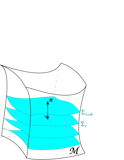
Figure 3.1: Spacetime foliation by a family of spacelike hypersurfaces $\Sigma_{t}$. The $\Sigma_{t}$’s can be considered as the level sets of some smooth scalar field $t$, such that the gradient $\bm{\mathrm{d}}t$ is timelike.

3.2 Spacetime foliation $\Sigma_{t}$

The spacetime (or at least the part of it under study, in the vicinity of the null hypersurface ${\mathcal{H}}$) is supposed to be foliated by a continuous family of spacelike hypersurfaces $(\Sigma_{t})$, labeled by the time coordinate $t$ (Fig. 3.1). The $\Sigma_{t}$’s can be considered as the level sets of some smooth scalar field $t$, such that the gradient $\bm{\mathrm{d}}t$ is timelike. We denote by $\bm{n}$ the future directed timelike unit vector normal to $\Sigma_{t}$. It can be identified with the 4-velocity of the class of observers whose worldlines are orthogonal to $\Sigma_{t}$ (Eulerian observers). By definition the 1-form $\underline{\bm{n}}$ dual to $\bm{n}$ [cf. notation (1.10)] is parallel to the gradient of the scalar field $t$:

$$\framebox{$\displaystyle\underline{\bm{n}}=-N\,\bm{\mathrm{d}}t$}.$$ (3.1)

The proportionality factor $N$ is called the lapse function. It ensures that $\bm{n}$ satisfies the normalization relation

$$\bm{n}\cdot\bm{n}=\langle\underline{\bm{n}},\bm{n}\rangle=-1.$$ (3.2)

The metric $\bm{\gamma}$ induced by $\bm{g}$ on each hypersurface $\Sigma_{t}$ (first fundamental form of $\Sigma_{t}$) is given by

$$\framebox{$\displaystyle\bm{\gamma}=\bm{g}+\underline{\bm{n}}\otimes\underline{\bm{n}}$}.$$ (3.3)

Since $\Sigma_{t}$ is assumed to be spacelike, $\bm{\gamma}$ is a positive definite (i.e. Riemannian) metric. Let us stress that the writing (3.3) is fully 4-dimensional and does not restrict the definition of $\bm{\gamma}$ to ${\mathcal{T}}_{p}(\Sigma_{t})$: it is a bilinear form on ${\mathcal{T}}_{p}({\mathcal{M}})$. The endomorphism ${\mathcal{T}}_{p}({\mathcal{M}})\rightarrow{\mathcal{T}}_{p}({\mathcal{M}})$ canonically associated with the bilinear form $\bm{\gamma}$ by the metric $\bm{g}$ [cf. notation (1.12)] is the orthogonal projector onto $\Sigma_{t}$:

$$\vec{\bm{\gamma}}=\bm{1}+\langle\underline{\bm{n}},.\rangle\bm{n}$$ (3.4)

(in index notation: $\gamma^{\alpha}_{\ \,\beta}=\delta^{\alpha}_{\ \,\beta}+n^{\alpha}n_{\beta}$, whereas (3.3) writes $\gamma_{\alpha\beta}=g_{\alpha\beta}+n_{\alpha}n_{\beta}$).

The existence of the orthogonal projector $\vec{\bm{\gamma}}$ makes a great difference with the case of null hypersurfaces, for which such an object does not exist (cf. Remark 2.3). In particular we can use it to map any multilinear form on ${\mathcal{T}}_{p}(\Sigma_{t})$ into a multilinear form on ${\mathcal{T}}_{p}({\mathcal{M}})$, which is in the direction inverse of that of the pull-back mapping induced by the embedding of $\Sigma_{t}$ in ${\mathcal{M}}$. We denote this mapping ${\mathcal{T}}_{p}^{*}(\Sigma_{t})\rightarrow{\mathcal{T}}_{p}^{*}({\mathcal{M}})$ by $\vec{\bm{\gamma}}^{*}$ and make it explicit as follows: given a $n$-linear form $\bm{A}$ on ${\mathcal{T}}_{p}(\Sigma_{t})$, $\vec{\bm{\gamma}}^{*}\bm{A}$ is the $n$-linear form acting on ${\mathcal{T}}_{p}({\mathcal{M}})^{n}$ defined by

$$\framebox{$\displaystyle\begin{array}[]{cccc}\vec{\bm{\gamma}}^{*}\bm{A}:&{\mathcal{T}}_{p}({\mathcal{M}})^{n}&\longrightarrow&\mathbb{R}\\ &(\bm{v}_{1},\ldots,\bm{v}_{n})&\longmapsto&\bm{A}\left(\vec{\bm{\gamma}}(\bm{v}_{1}),\ldots,\vec{\bm{\gamma}}(\bm{v}_{n})\right).\end{array}$}$$ (3.5)

Actually we extend the above definition to all multilinear forms $\bm{A}$ on ${\mathcal{T}}_{p}({\mathcal{M}})$ and not only those restricted to ${\mathcal{T}}_{p}(\Sigma_{t})$. The index version of this definition is

$$(\vec{\gamma}^{*}A)_{\alpha_{1}\ldots\alpha_{n}}=A_{\mu_{1}\ldots\mu_{n}}\gamma^{\mu_{1}}_{\ \ \ \alpha_{1}}\cdots\gamma^{\mu_{n}}_{\ \ \ \alpha_{n}}.$$ (3.6)

In particular, we have

$$\vec{\bm{\gamma}}^{*}\bm{g}=\bm{\gamma}\qquad\mbox{and}\qquad\vec{\bm{\gamma}}^{*}\underline{\bm{n}}=0.$$ (3.7)

There exists a unique (torsion-free) connection on $\Sigma_{t}$ associated with the metric $\bm{\gamma}$, which we denote by $\bm{D}$: $\bm{D}\bm{\gamma}=0$. If we consider a generic tensor field $\bm{T}$ of type $\left({p\atop q}\right)$ lying on $\Sigma_{t}$ (i.e. such that its contraction with the normal $\bm{n}$ on any of its indices vanishes), then, from a 4-dimensional point of view, the covariant derivative $\bm{D}\bm{T}$ can be expressed as the full orthogonal projection of the spacetime covariant derivative $\bm{\nabla}\bm{T}$ on $\Sigma_{t}$ [see Eq. (1.2)]:

$$\framebox{$\displaystyle D_{\gamma}T^{\alpha_{1}\ldots\alpha_{p}}_{\ \qquad\beta_{1}\ldots\beta_{q}}=\gamma_{\ \ \,\mu_{1}}^{\alpha_{1}}\,\cdots\gamma_{\ \ \,\mu_{p}}^{\alpha_{p}}\,\gamma_{\ \ \,\beta_{1}}^{\nu_{1}}\,\cdots\gamma_{\ \ \,\beta_{q}}^{\nu_{q}}\,\gamma_{\ \ \,\gamma}^{\sigma}\,\nabla_{\sigma}T^{\mu_{1}\ldots\mu_{p}}_{\ \qquad\nu_{1}\ldots\nu_{q}}$}.$$ (3.8)

In the following, we shall make extensive use of this formula, without making explicit mention. In the special case of a tensor of type $\left({0\atop q}\right)$, i.e. a multilinear form, the definition of $\bm{D}\bm{T}$ amounts to, thanks to Eq. (3.6),

$$\bm{D}\bm{T}=\vec{\bm{\gamma}}^{*}\bm{\nabla}\bm{T}.$$ (3.9)

3.3 Weingarten map and extrinsic curvature

As for the hypersurface ${\mathcal{H}}$, the “bending” of each hypersurface $\Sigma_{t}$ in ${\mathcal{M}}$ is described by the Weingarten map which associates with each vector tangent to $\Sigma_{t}$ the covariant derivative (with respect to the ambient connection $\bm{\nabla}$) of the unit normal $\bm{n}$ along this vector [compare with Eq. (2.50)]:

$$\begin{array}[]{cccc}\bm{\mathcal{K}}:&{\mathcal{T}}_{p}(\Sigma_{t})&\longrightarrow&{\mathcal{T}}_{p}(\Sigma_{t})\\ &\bm{v}&\longmapsto&\bm{\nabla}_{\bm{v}}\,\bm{n}.\end{array}$$ (3.10)

The computations presented in Sec. 2.6 for the Weingarten map $\bm{\chi}$ of ${\mathcal{H}}$ can be repeated here, by simply replacing the normal $\bm{\ell}$ by the normal $\bm{n}$, the field $u$ by the field $t$ and the coefficient $\e^{\rho}$ by $-N$ [compare Eqs. (2.14) and (3.1)]. They then show that $\bm{\mathcal{K}}$ is well defined (i.e. its image is in ${\mathcal{T}}_{p}(\Sigma_{t})$) and that it is self-adjoint with respect to the metric $\bm{\gamma}$. A difference with the Weingarten map $\bm{\chi}$ of ${\mathcal{H}}$ is that the Weingarten map $\bm{\mathcal{K}}$ can be naturally extended to ${\mathcal{T}}_{p}({\mathcal{M}})$ thanks to the orthogonal projector $\vec{\bm{\gamma}}$ [Eq. (3.4)], which did not exist for ${\mathcal{H}}$ (cf. Remark 2.3), by setting

$$\begin{array}[]{cccc}\bm{\mathcal{K}}:&{\mathcal{T}}_{p}({\mathcal{M}})&\longrightarrow&{\mathcal{T}}_{p}(\Sigma_{t})\\ &\bm{v}&\longmapsto&\bm{\nabla}_{\vec{\bm{\gamma}}(\bm{v})}\,\bm{n},\end{array}$$ (3.11)

or in index notation:

$$\mathcal{K}^{\alpha}_{\ \,\beta}=\nabla_{\mu}n^{\alpha}\;\gamma^{\mu}_{\ \,\beta}.$$ (3.12)

We then define the extrinsic curvature tensor $\bm{K}$ of the hypersurface $\Sigma_{t}$ as minus the second fundamental form [compare with Eq. (2.57)]:

$$\begin{array}[]{cccc}\bm{K}:&{\mathcal{T}}_{p}({\mathcal{M}})\times{\mathcal{T}}_{p}({\mathcal{M}})&\longrightarrow&\mathbb{R}\\ &(\bm{u},\bm{v})&\longmapsto&-\bm{u}\cdot\bm{\mathcal{K}}(\bm{v}),\end{array}$$ (3.13)

or in index notation

$$K_{\alpha\beta}=-\nabla_{\mu}n_{\alpha}\;\gamma^{\mu}_{\ \,\beta}.$$ (3.14)

Since the image of $\bm{\mathcal{K}}$ is in ${\mathcal{T}}_{p}(\Sigma_{t})$, we can write $\bm{K}(\bm{u},\bm{v})=-\,\vec{\bm{\gamma}}(\bm{u})\cdot\bm{\mathcal{K}}(\vec{\bm{\gamma}}(\bm{v}))$. It follows then immediately from the self-adjointness of $\bm{\mathcal{K}}$ that $\bm{K}$ is symmetric and that the following relation holds:

$$K_{\alpha\beta}=-\nabla_{\mu}n_{\nu}\;\gamma^{\mu}_{\ \,\alpha}\gamma^{\nu}_{\ \,\beta},$$ (3.15)

which we can write, thanks to Eq. (3.6) and the symmetry of $\bm{K}$,

$$\framebox{$\displaystyle\bm{K}=-\,\vec{\bm{\gamma}}^{*}\bm{\nabla}\underline{\bm{n}}$}.$$ (3.16)

Replacing in Eq. (3.14) $n_{\alpha}$ by its expression (3.1) in terms of the gradient of $t$ leads to

$$K_{\alpha\beta} = \nabla_{\mu}(N\nabla_{\alpha}t)\;\gamma^{\mu}_{\ \,\beta}=\left(\nabla_{\mu}N\nabla_{\alpha}t+N\nabla_{\mu}\nabla_{\alpha}t\right)\gamma^{\mu}_{\ \,\beta}$$ (3.17)

$$= \left(\nabla_{\mu}N\nabla_{\alpha}t+N\nabla_{\alpha}\nabla_{\mu}t\right)\gamma^{\mu}_{\ \,\beta}=D_{\beta}N\nabla_{\alpha}t+N\nabla_{\alpha}\left(-N^{-1}n_{\mu}\right)\gamma^{\mu}_{\ \,\beta}$$

$$= -n_{\alpha}N^{-1}D_{\beta}N-N\nabla_{\alpha}(N^{-1})\;\underbrace{n_{\mu}\gamma^{\mu}_{\ \,\beta}}_{=0}-\nabla_{\alpha}n_{\mu}\gamma^{\mu}_{\ \,\beta}$$

$$= -n_{\alpha}D_{\beta}\ln N-\nabla_{\alpha}n_{\mu}\,\delta^{\mu}_{\ \,\beta}-\underbrace{\nabla_{\alpha}n_{\mu}\,n^{\mu}}_{=0}n_{\beta}.$$

Hence

$$\framebox{$\displaystyle K_{\alpha\beta}=-\nabla_{\alpha}n_{\beta}-n_{\alpha}\,D_{\beta}\ln N$}.$$ (3.18)

or, taking into account the symmetry of $\bm{K}$ and Eq. (1.9)

$$\framebox{$\displaystyle\bm{K}=-\bm{\nabla}\underline{\bm{n}}-\bm{D}\ln N\otimes\underline{\bm{n}}$}.$$ (3.19)

In the following, we will make extensive use of this formula, without explicitly mentioning it. Inserting $\bm{n}$ as the second argument in the bilinear form (3.19) and using $\bm{K}(.,\bm{n})=0$ as well as $\langle\underline{\bm{n}},\bm{n}\rangle=-1$ results in the important formula giving the 4-acceleration of the Eulerian observers:

$$\framebox{$\displaystyle\bm{\nabla}_{\bm{n}}\,\underline{\bm{n}}=\bm{D}\ln N$}.$$ (3.20)

Another useful formula relates $\bm{K}$ to the Lie derivative of the spatial metric $\bm{\gamma}$ along the normal $\bm{n}$:

$$\framebox{$\displaystyle\bm{K}=-{1\over 2}\bm{\mathcal{L}}_{\bm{\bm{n}}}\,\bm{\gamma}$}.$$ (3.21)

This formula follows from Eq. (3.19) and the symmetry of $\bm{K}$ by a direct computation, provided that the Lie derivative along $\bm{n}$ is expressed in terms of the connection $\bm{\nabla}$ via Eq. (1.2.1): $({\mathcal{L}}_{\bm{\bm{n}}}\,\gamma)_{\alpha\beta}=n^{\mu}\nabla_{\mu}\gamma_{\alpha\beta}+\gamma_{\mu\beta}\nabla_{\alpha}n^{\mu}+\gamma_{\alpha\mu}\nabla_{\beta}n^{\mu}$.

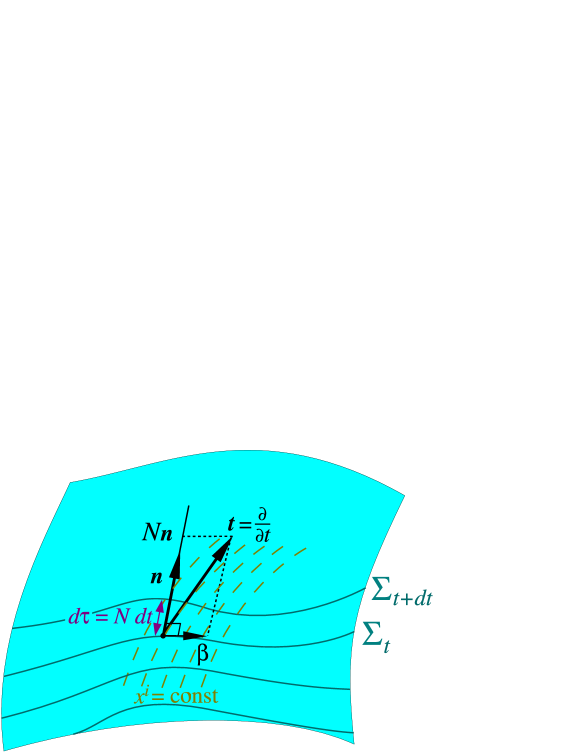
Figure 3.2: Constant spatial coordinate lines $x^{i}={\rm const}$ cutting across the foliation $(\Sigma_{t})$ and defining the coordinate time vector $\bm{t}$ and the shift vector $\bm{\beta}$. Also represented are the the unit normal to each hypersurface $\Sigma_{t}$, $\bm{n}$, and the lapse function $N$ as giving the metric distance $d\tau$ between two neighboring hypersurfaces $\Sigma_{t}$ and $\Sigma_{t+dt}$ via $d\tau=N\,dt$.

3.4 3+1 coordinates and shift vector

We may introduce on ${\mathcal{M}}$ a coordinate system adapted to the $(\Sigma_{t})$ foliation by considering on each hypersurface $\Sigma_{t}$ a coordinate system $(x^{i})$, such that $(x^{i})$ varies smoothly from one hypersurface to the next one. Then, $(x^{\alpha})=(x^{0}=t,x^{i})$ constitutes a well behaved coordinate of ${\mathcal{M}}$. The coordinate time vector of this system is

$$\bm{t}:=\frac{\partial}{\partial t}$$ (3.22)

and is such that each spatial coordinate $x^{i}$ is constant along its field lines. $\bm{t}$ can be seen as a vector “dual” to the gradient 1-form $\bm{\mathrm{d}}t$, in the sense that

$$\langle\bm{\mathrm{d}}t,\bm{t}\rangle=1.$$ (3.23)

Then, from Eq. (3.1), $\bm{n}\cdot\bm{t}=-N$ and we have the orthogonal 3+1 decomposition

$$\framebox{$\displaystyle\bm{t}=N\bm{n}+\bm{\beta}$}\qquad\mbox{with}\quad\bm{n}\cdot\bm{\beta}=0.$$ (3.24)

The vector $\bm{\beta}:=\vec{\bm{\gamma}}(\bm{t})$ is called the shift vector of the coordinate system $(x^{\alpha})$. The vectors $\bm{t}$ and $\bm{\beta}$ are represented in Fig. 3.2. Given a choice of the coordinates $(x^{i})$ in an initial slice $\Sigma_{0}$, fixing the lapse function $N$ and shift vector $\bm{\beta}$ on every $\Sigma_{t}$ fully determines the coordinates $(x^{\alpha})$ in the portion of ${\mathcal{M}}$ covered by these coordinates. We refer the reader to Ref. [152] for an extended discussion of the choice of coordinates based on the lapse and the shift.

The components $g_{\alpha\beta}$ of the metric tensor $\bm{g}$ with respect to the coordinates $(t,x^{i})$ are expressible in terms of the lapse $N$, the components $\beta^{i}$ of the shift vector and the components $\gamma_{ij}$ of the spatial metric, according to

$$g_{\mu\nu}\,dx^{\mu}\,dx^{\nu}=-N^{2}dt^{2}+\gamma_{ij}(dx^{i}+\beta^{i}dt)(dx^{j}+\beta^{j}dt).$$ (3.25)

Example 3.1

Lapse and shift of Eddington-Finkelstein coordinates.
Returning to Example 2.5 (Schwarzschild spacetime in Eddington-Finkelstein coordinates), the lapse function and shift vector of the 3+1 Eddington-Finkelstein coordinates are obtained by comparing Eqs. (3.25) and (2.34):

$$N=\frac{1}{\sqrt{1+2m/r}},$$ (3.26)

$$\beta^{\alpha}=\left(0,\frac{1}{1+r/(2m)},0,0\right)\quad\mbox{and}\quad\beta_{\alpha}=\left(\frac{4m^{2}}{r(r+2m)},\frac{2m}{r},0,0\right).$$ (3.27)

Note that, on ${\mathcal{H}}$ ($r=2m$), $N\stackrel{{\scriptstyle{\mathcal{H}}}}{{=}}1/\sqrt{2}$ and $\beta^{r}\stackrel{{\scriptstyle{\mathcal{H}}}}{{=}}1/2$. The expression for the unit timelike normal to the hypersurfaces $\Sigma_{t}$ is deduced from $N$ and $\bm{\beta}$:

$$n^{\alpha}=\left(\sqrt{1+\frac{2m}{r}},-\frac{2m}{r\sqrt{1+\frac{2m}{r}}},0,0\right),\quad n_{\alpha}=\left(-\frac{1}{\sqrt{1+\frac{2m}{r}}},0,0,0\right).$$ (3.28)

3.5 3+1 decomposition of the Riemann tensor

We present here the expression of the spacetime Riemann tensor $\mathrm{\bf Riem}$ (cf. Sec. 1.2.2) in terms of 3+1 objects, in particular the Riemann tensor ${}^{3}\mathrm{\bf Riem}$ of the connection $\bm{D}$ associated with the spatial metric $\bm{\gamma}$. This is a step required to get a 3+1 decomposition of the Einstein equation in next section. Moreover, this allows to gain intuition on the analogous (but null) decomposition that will be introduced in Sec. 6, when studying the dynamics of a null hypersurface.

As a general strategy, calculations start from the 3-dimensional objects and then use is made of Eqs. (3.8) and (3.3), together with the Ricci identity (1.14). Since these techniques will be explicitly exposed in Sec. 6, we present the following results without proof (see, for instance, Ref. [171]). The 3+1 writing of the spacetime Riemann tensor thus obtained can be viewed as various orthogonal projections of $\mathrm{\bf Riem}$ onto the hypersurface $\Sigma_{t}$ and along the normal $\bm{n}$:

$$\gamma^{\alpha}_{\ \,\mu}\gamma^{\nu}_{\ \,\beta}\gamma^{\rho}_{\ \,\gamma}\gamma^{\sigma}_{\ \,\delta}\,R^{\mu}_{\ \,\nu\rho\sigma} = {}^{3}\!R^{\alpha}_{\ \,\beta\gamma\delta}+K^{\alpha}_{\ \,\gamma}K_{\beta\delta}-K^{\alpha}_{\ \,\delta}K_{\beta\gamma}.$$ (3.29)

$$\gamma^{\alpha}_{\ \,\mu}\gamma^{\nu}_{\ \,\beta}\gamma^{\rho}_{\ \,\gamma}n^{\sigma}\,R^{\mu}_{\ \,\nu\rho\sigma} = D_{\beta}K^{\alpha}_{\ \,\gamma}-D^{\alpha}K_{\beta\gamma}$$ (3.30)

$$\gamma_{\alpha\mu}n^{\nu}\gamma^{\rho}_{\ \,\beta}n^{\sigma}\,R^{\mu}_{\ \,\nu\rho\sigma} = \frac{1}{N}\mathcal{L}_{(N\bm{n})}K_{\alpha\beta}+K_{\alpha\mu}K^{\mu}_{\ \,\beta}+\frac{1}{N}D_{\alpha}D_{\beta}N.$$ (3.31)

From the symmetries of the Riemann tensor, all the other contractions involving $\bm{n}$ either are equivalent to one of the Eqs. (3.30)-(3.31), or vanish. For instance, a contraction with three times $\bm{n}$ would be zero. Equation (3.29) is known as the Gauss equation, and Eq. (3.30) as the Codazzi equation. The third equation, (3.31), is sometimes called the Ricci equation [not to be confused with the Ricci identity (1.14)].

The Gauss and Codazzi equations do not involve any second order derivative of the metric tensor $\bm{g}$ in a timelike direction. They constitute the necessary and sufficient conditions for the hypersurface $\Sigma_{t}$, endowed with a 3-metric $\bm{\gamma}$ and an extrinsic curvature $\bm{K}$, to be a submanifold of $(\mathcal{M},\bm{g})$. Contracted versions of the Gauss and Codazzi equations turn out to be very useful, especially in the 3+1 writing of the Einstein equation. Contracting the Gauss equation (3.29) on the indices $\alpha$ and $\gamma$ leads to an expression that makes appear the Ricci tensors $\bm{R}$ and ${}^{3}\!\bm{R}$ associated with $\bm{g}$ and $\bm{\gamma}$, respectively [cf. Eq. (1.17)]

$$\gamma^{\mu}_{\ \,\alpha}\gamma^{\nu}_{\ \,\beta}R_{\mu\nu}+\gamma_{\alpha\mu}n^{\nu}\gamma^{\rho}_{\ \,\beta}n^{\sigma}\,R^{\mu}_{\ \,\nu\rho\sigma}={}^{3}\!R_{\alpha\beta}+KK_{\alpha\beta}-K_{\alpha\mu}K^{\mu}_{\ \,\beta},$$ (3.32)

where $K$ is the trace of $\bm{K}$, $K^{\mu}_{\mu}$. Taking the trace of this equation with respect to $\bm{\gamma}$, leads to an expression that involves the Ricci scalars $R:=g^{\mu\nu}R_{\mu\nu}$ and ${}^{3}\!R:=\gamma^{\mu\nu}{}^{3}\!R_{\mu\nu}$, again respectively associated with $\bm{g}$ and $\bm{\gamma}$:

$$R+2R_{\mu\nu}n^{\mu}n^{\nu}={}^{3}\!R+K^{2}-K_{\mu\nu}K^{\mu\nu}.$$ (3.33)

This formula, which relates the intrinsic curvature ${}^{3}\!R$ and the extrinsic curvature $\bm{K}$ of $\Sigma_{t}$, can be seen as a generalization to the 4-dimensional case of Gauss’ famous Theorema egregium (see e.g. Ref. [26]). On the other side, contracting the Codazzi equation on the indices $\alpha$ and $\gamma$ leads to

$$\gamma^{\mu}_{\ \,\alpha}n^{\nu}R_{\mu\nu}=D_{\alpha}K-D^{\mu}K_{\alpha\mu}.$$ (3.34)

3.6 3+1 Einstein equation

We are now in position of presenting the 3+1 splitting of Einstein equation:

$$\framebox{$\displaystyle\bm{R}-\frac{1}{2}R\bm{g}=8\pi\bm{T}$},$$ (3.35)

where $\bm{T}$ is the total (matter + electromagnetic field) energy-momentum tensor. The 3+1 decomposition of the latter is

$$\bm{T}=E\,\bm{n}\otimes\bm{n}+\bm{n}\otimes\bm{J}+\bm{J}\otimes\bm{n}+\bm{S},$$ (3.36)

where the energy density $E$, the momentum density $\bm{J}$ and the strain tensor $\bm{S}$, all of them as measured by the Eulerian observer of 4-velocity $\bm{n}$, are given by the following projections $E:=T_{\mu\nu}n^{\mu}n^{\nu}$, $J_{\alpha}:=-\gamma_{\alpha}^{\ \,\mu}T_{\mu\nu}n^{\nu}$, $S_{\alpha\beta}:=\gamma_{\alpha}^{\ \,\mu}\gamma_{\beta}^{\ \,\nu}T_{\mu\nu}$.

Einstein equation (3.35) splits into three equations by using, respectively, (i) the twice contracted Gauss equation (3.33), (ii) the contracted Codazzi equation (3.34), (iii) the combination of the Ricci equation (3.31) with the contracted Gauss equation (3.32):

$$\framebox{$\displaystyle{}^{3}\!R+K^{2}-K_{\mu\nu}K^{\mu\nu}=16\pi E$},$$ (3.37)

$$\framebox{$\displaystyle D^{\mu}K_{\alpha\mu}-D_{\alpha}K=8\pi J_{\alpha}$},$$ (3.38)

$$\framebox{$\displaystyle\begin{array}[]{rcl}\mathcal{L}_{(N\bm{n})}K_{\alpha\beta}&=&\displaystyle-D_{\alpha}D_{\beta}N+N\Big{\{}{}^{3}\!R_{\alpha\beta}-2K_{\alpha\mu}K^{\mu}_{\ \,\beta}+KK_{\alpha\beta}\\ &&\displaystyle+4\pi\left[(S-E)\gamma_{\alpha\beta}-2S_{\alpha\beta}\right]\Big{\}}\end{array}$}\ .$$ (3.39)

These equations are known as the Hamiltonian constraint, the momentum constraint and the dynamical 3+1 equations, respectively.

The Hamiltonian and momentum constraints do not contain any second order derivative of the metric in a timelike direction, contrary to Eq. (3.39) [remember that $\bm{K}$ is already a first order derivative of the metric in the timelike direction $\bm{n}$, according to Eq. (3.21)]. Therefore they are not associated with the dynamical evolution of the gravitational field and represent constraints to be satisfied by $\bm{\gamma}$ and $\bm{K}$ on each hypersurface $\Sigma_{t}$.

The dynamical equation (3.39) can be written explicitly as a time evolution equation, once a 3+1 coordinate system $(t,x^{i})$ is introduced, as in Sec. 3.4. Then $N\bm{n}$ is expressible in terms of the coordinate time vector $\bm{t}$ and the shift vector $\bm{\beta}$ associated with these coordinates: $N\bm{n}=\bm{t}-\bm{\beta}$ [cf. Eq. (3.24)], so that the Lie derivative in the left-hand side of Eq. (3.39) can be written as

$$\bm{\mathcal{L}}_{(N\bm{n})}=\bm{\mathcal{L}}_{\bm{\bm{t}}}\,-\bm{\mathcal{L}}_{\bm{\bm{\beta}}}\,.$$ (3.40)

Now, if one uses tensor components with respect to the coordinates $(x^{i})$, ${\mathcal{L}}_{\bm{\bm{t}}}\,K_{ij}={\partial K_{ij}/\partial t}$, Eq. (3.39) becomes

$$\framebox{$\displaystyle\begin{array}[]{rcl}\displaystyle\frac{\partial}{\partial t}K_{ij}-{\mathcal{L}}_{\bm{\bm{\beta}}}\,K_{ij}&=&\displaystyle-D_{i}D_{j}N+N\Big{\{}{}^{3}\!R_{ij}-2K_{ik}K^{k}_{\ \,j}+KK_{ij}\\ &&\displaystyle+4\pi\left[(S-E)\gamma_{ij}-2S_{ij}\right]\Big{\}}\end{array}$}.$$ (3.41)

Similarly, the relation (3.21) between $\bm{K}$ and $\bm{\mathcal{L}}_{\bm{\bm{n}}}\,\bm{\gamma}$ becomes

$$\framebox{$\displaystyle\frac{\partial}{\partial t}\gamma_{ij}-{\mathcal{L}}_{\bm{\bm{\beta}}}\,\gamma_{ij}=-2NK_{ij}$},$$ (3.42)

where one may use the following identity [cf. Eq. (1.2.1)]: ${\mathcal{L}}_{\bm{\bm{\beta}}}\,\gamma_{ij}=D_{i}\beta_{j}+D_{j}\beta_{i}$.

3.7 Initial data problem

In view of the above equations, the standard procedure of numerical relativity consists in firstly specifying the values of $\bm{\gamma}$ and $\bm{K}$ on some initial spatial hypersurface $\Sigma_{0}$ (Cauchy surface), and then evolving them according to Eqs. (3.41) and (3.42). For this scheme to be valid, the initial data must satisfy the constraint Eqs. (3.37)-(3.38). The problem of finding pairs $(\bm{\gamma},\bm{K})$ on $\Sigma_{0}$ satisfying these constraints constitutes the initial data problem of 3+1 general relativity.

The existence of a well-posed initial value formulation for Einstein equation, first established by Y. Choquet-Bruhat more than fifty years ago [70], provides fundamental insight for a number of issues in general relativity (see e.g. Refs. [68, 22] for a mathematical account). In this article we aim at underlining those aspects related with the numerical construction of astrophysically relevant spacetimes containing black holes. In this sense, the 3+1 formalism constitutes a particularly convenient and widely extended approach to the problem (for other numerical approaches, see for instance [96, 97, 169]). Consequently, the first step in this numerical approach consists in generating appropriate initial data which correspond to astrophysically realistic situations. For a review on the numerical aspects of this initial data problem see [51, 135].

If one chooses to excise a sphere in the spatial surface $\Sigma_{t}$ for it to represent the horizon of a black hole, appropriate boundary conditions in this inner boundary must be imposed when solving the constraint Eqs. (3.37)-(3.38). This particular aspect of the initial data problem constitutes one of the main applications of the subject studied here, and will be developed in Sec. 11. In order to carry out such a discussion, the conformal decomposition of the initial data introduced by Lichnerowicz [113], particularly successful in the generation of initial data, will be presented in Sec. 10.

4 3+1-induced foliation of null hypersurfaces

4.1 Introduction

In Secs. 2.6 and 2.7, we have introduced two geometrical objects on the 3-manifold ${\mathcal{H}}$: the Weingarten map $\bm{\chi}$ and the second fundamental form $\bm{\Theta}$. These objects are unique up to some rescaling of the null normal $\bm{\ell}$ to ${\mathcal{H}}$. Following Carter [41, 42, 43], we would like to consider these objects as 4-dimensional quantities, i.e. to extend their definitions from the 3-manifold ${\mathcal{H}}$ to the 4-manifold ${\mathcal{M}}$ (or at least to the vicinity of ${\mathcal{H}}$, as discussed in Sec. 2.3). The benefit of such an extension is an easier manipulation of these objects, as ordinary tensors on ${\mathcal{M}}$, which will facilitate the connection with the geometrical objects of the 3+1 slicing. In particular this avoids the introduction of special coordinate systems and complicated notations. For instance, one would like to define easily something like the type $\left(0\atop 3\right)$ tensor $\bm{\nabla}\bm{\Theta}$, where $\bm{\nabla}$ is the spacetime covariant derivative. At the present stage, this not possible even when restricting the definition of $\bm{\nabla}\bm{\Theta}$ to ${\mathcal{H}}$, because there is no unique covariant derivation associated with the induced metric $\bm{q}$, since the latter is degenerate.

We have already noticed that, from the null structure of ${\mathcal{H}}$ alone, there is no canonical mapping from vectors of ${\mathcal{M}}$ to vectors of ${\mathcal{H}}$, and in particular no orthogonal projector (Remarks 2.1 and 2.3). Such a mapping would have provided natural four-dimensional extensions of the forms defined on ${\mathcal{H}}$. Actually in order to define a projector onto ${\mathcal{T}}_{p}({\mathcal{H}})$, we need some direction transverse to ${\mathcal{H}}$, i.e. some vector of ${\mathcal{T}}_{p}({\mathcal{M}})$ not belonging to ${\mathcal{T}}_{p}({\mathcal{H}})$. We may then define a projector along this transverse direction. The problem with null hypersurfaces is that there is no canonical transverse direction since the normal direction is not transverse but tangent.

However if we take into account the foliation provided by some family of spacelike hypersurfaces $(\Sigma_{t})$ in the standard 3+1 formalism introduced in Sec. 3, we have some extra-structure on ${\mathcal{M}}$. We may then use it to define unambiguously a transverse direction to ${\mathcal{H}}$ and an associated projector $\bm{\Pi}$. Moreover this transverse direction will be, by construction, well suited to the 3+1 decomposition.

4.2 3+1-induced foliation of ${\mathcal{H}}$ and normalization of $\bm{\ell}$

In the general case, each spacelike hypersurface $\Sigma_{t}$ of the 3+1 slicing discussed in Sec. 3 intersects the null hypersurface ${\mathcal{H}}$ on some 2-dimensional surface ${\mathcal{S}}_{t}$ (cf. Fig. 4.1):

$$\framebox{$\displaystyle{\mathcal{S}}_{t}:={\mathcal{H}}\cap\Sigma_{t}$}.$$ (4.1)

More generally, considering some null foliation $({\mathcal{H}}_{u})$ in the vicinity of ${\mathcal{H}}$ (cf. Sec. 2.3), we define the 2-surface family $({\mathcal{S}}_{t,u})$ by

$${\mathcal{S}}_{t,u}:={\mathcal{H}}_{u}\cap\Sigma_{t}.$$ (4.2)

${\mathcal{S}}_{t}$ is then nothing but the element ${\mathcal{S}}_{t,u=1}$ of this family. $({\mathcal{S}}_{t,u})$ constitutes a foliation of ${\mathcal{M}}$ (in the vicinity of ${\mathcal{H}}$) by 2-surfaces. This foliation is of type null-timelike in the terminology of the 2+2 formalism [96, 98].

A local characterization of ${\mathcal{S}}_{t}$ follows from Eq. (2.2) and the definition of $\Sigma_{t}$ as the level set of some scalar field $t$:

$$\forall p\in{\mathcal{M}},\quad p\in{\mathcal{S}}_{t}\iff u(p)=1\ \ \mbox{and}\ \ t(p)=t.$$ (4.3)

The subspace ${\mathcal{T}}_{p}({\mathcal{S}}_{t})$ of vectors tangent to ${\mathcal{S}}_{t}$ at some point $p\in{\mathcal{S}}_{t}$ is then characterized in terms of the gradients of the scalar fields $u$ and $t$ by

$$\forall\bm{v}\in{\mathcal{T}}_{p}({\mathcal{M}}),\quad\bm{v}\in{\mathcal{T}}_{p}({\mathcal{S}}_{t})\iff\langle\bm{\mathrm{d}}u,\bm{v}\rangle=0\ \ \mbox{and}\ \ \langle\bm{\mathrm{d}}t,\bm{v}\rangle=0.$$ (4.4)

As a submanifold of $\Sigma_{t}$, each ${\mathcal{S}}_{t}$ is necessarily a spacelike surface. Until Sec. 7, we make no assumption on the topology of ${\mathcal{S}}_{t}$, although we picture it as a closed (i.e. compact without boundary) manifold (Fig. 4.1). In the absence of global assumptions on ${\mathcal{S}}_{t}$ or ${\mathcal{H}}$, we define the exterior (resp. interior) of ${\mathcal{S}}_{t}$, as the region of $\Sigma_{t}$ for which $u>1$ (resp. $u<1$). In the case another criterion is available to define the exterior of ${\mathcal{S}}_{t}$ (e.g. if ${\mathcal{S}}_{t}$ has the topology of $\mathbb{S}^{2}$, $\Sigma_{t}$ is asymptotically flat and the exterior of ${\mathcal{S}}_{t}$ is defined as the connected component of $\Sigma_{t}\setminus{\mathcal{S}}_{t}$ which contains the asymptotically flat region), we can always change the definition of $u$ to make coincide the two definitions of exterior.

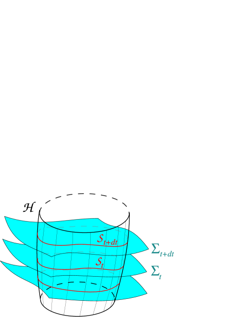
Figure 4.1: Foliation $({\mathcal{S}}_{t})$ of the null hypersurface ${\mathcal{H}}$ induced by the spacetime foliation $(\Sigma_{t})$ of the 3+1 formalism.

The ${\mathcal{S}}_{t}$’s constitute a foliation of ${\mathcal{H}}$. The coordinate $t$ can then be used as a parameter, in general non-affine, along each null geodesic generating ${\mathcal{H}}$ (cf. Sec. 2.5). Thanks to it, we can normalize the null normal $\bm{\ell}$ of ${\mathcal{H}}$ by demanding that $\bm{\ell}$ is the tangent vector associated with this parametrization of the null generators:

$$\ell^{\alpha}={dx^{\alpha}\over dt}.$$ (4.5)

An equivalent phrasing of this is demanding that $\bm{\ell}$ is a vector field “dual” to the 1-form $\bm{\mathrm{d}}t$ (equivalently, the function $t$ can be regarded as a coordinate compatible with $\bm{\ell}$):

$$\framebox{$\displaystyle\langle\bm{\mathrm{d}}t,\bm{\ell}\rangle=\bm{\nabla}_{\bm{\ell}}\,t=1$}.$$ (4.6)

A geometrical consequence of this choice is that the 2-surface ${\mathcal{S}}_{t+\delta t}$ is obtained from the 2-surface ${\mathcal{S}}_{t}$ by a displacement $\delta t\bm{\ell}$ at each point of ${\mathcal{S}}_{t}$, as depicted in Fig. 4.2. Indeed consider a point $p$ in ${\mathcal{S}}_{t}$ and displace it by a infinitesimal quantity $\delta t\bm{\ell}$ to the point $p^{\prime}=p+\delta t\bm{\ell}$ (cf. Fig. 4.2). From the very definition of the gradient 1-form $\bm{\mathrm{d}}t$, the value of the scalar field $t$ at $p^{\prime}$ is

$$t(p^{\prime}) = t(p+\delta t\bm{\ell})=t(p)+\langle\bm{\mathrm{d}}t,\delta t\bm{\ell}\rangle=t(p)+\delta t\underbrace{\langle\bm{\mathrm{d}}t,\bm{\ell}\rangle}_{=1}$$ (4.7)

$$= t(p)+\delta t.$$

This last equality shows that $p^{\prime}\in{\mathcal{S}}_{t+\delta t}$. Hence the vector $\delta t\bm{\ell}$ carries the surface ${\mathcal{S}}_{t}$ into the neighboring one ${\mathcal{S}}_{t+\delta t}$. One says equivalently that the 2-surfaces $({\mathcal{S}}_{t})$ are Lie dragged by the null normal $\bm{\ell}$.

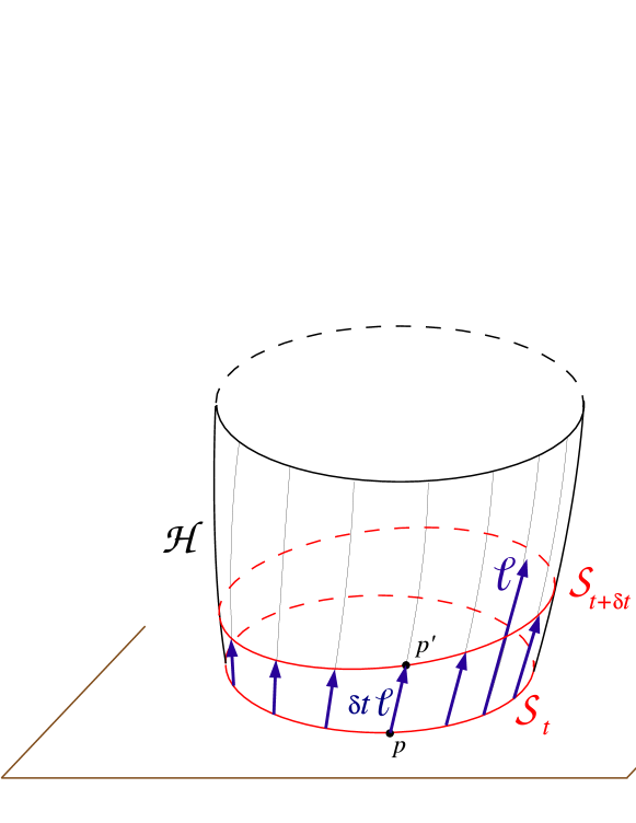
Figure 4.2: Lie transport of the surfaces ${\mathcal{S}}_{t}$ by the vector $\bm{\ell}$.

Let $\bm{s}$ be the unit vector of $\Sigma_{t}$, normal to ${\mathcal{S}}_{t}$ and directed toward the exterior of ${\mathcal{S}}_{t}$ (cf. Fig. 4.3); $\bm{s}$ obeys to the following properties:

$$\bm{s}\cdot\bm{s}=1,$$ (4.8)

$$\bm{n}\cdot\bm{s}=0,$$ (4.9)

$$\langle\bm{\mathrm{d}}u,\bm{s}\rangle>0,$$ (4.10)

$$\forall\bm{v}\in{\mathcal{T}}_{p}(\Sigma_{t}),\quad\bm{v}\in{\mathcal{T}}_{p}({\mathcal{S}}_{t})\iff\bm{s}\cdot\bm{v}=0.$$ (4.11)

Let us establish a simple expression of the null normal $\bm{\ell}$ in terms of the unit vectors $\bm{n}$ and $\bm{s}$. Let $\bm{b}\in{\mathcal{T}}_{p}(\Sigma_{t})$ be the orthogonal projection of $\bm{\ell}$ onto $\Sigma_{t}$: $\bm{b}:=\vec{\bm{\gamma}}(\bm{\ell})$ [cf. Eq. (3.4)]. Then $\bm{\ell}=a\bm{n}+\bm{b}$, with a coefficient $a$ to be determined. By means of Eq. (3.1), $\langle\bm{\mathrm{d}}t,\bm{\ell}\rangle=a/N$, so that the normalization condition (4.6) leads to $a=N$, hence

$$\bm{\ell}=N\bm{n}+\bm{b}.$$ (4.12)

For any vector $\bm{v}\in{\mathcal{T}}_{p}({\mathcal{S}}_{t})$, $\bm{\ell}\cdot\bm{v}=0$. Replacing $\bm{\ell}$ by the above expression and using $\bm{n}\cdot\bm{v}=0$ results in $\bm{b}\cdot\bm{v}=0$. Since this equality is valid for any $\bm{v}\in{\mathcal{T}}_{p}({\mathcal{S}}_{t})$, we deduce that $\bm{b}$ is a vector of $\Sigma_{t}$ which is normal to ${\mathcal{S}}_{t}$. It is then necessarily collinear to $\bm{s}$: $\bm{b}=\alpha\bm{s}$, with $\alpha=\bm{s}\cdot\bm{b}=\bm{s}\cdot\bm{\ell}=\langle\underline{\bm{\ell}},\bm{s}\rangle=e^{\rho}\langle\bm{\mathrm{d}}u,\bm{s}\rangle>0$, thanks to Eq. (4.10). The condition $\bm{\bm{\ell}}\cdot\bm{\bm{\ell}}=0$ then leads to $\alpha=N$, so that finally

$$\framebox{$\displaystyle\bm{\ell}=N(\bm{n}+\bm{s})$}.$$ (4.13)

In particular, the three vectors $\bm{\ell}$, $\bm{n}$ and $\bm{s}$ are coplanar (see Fig. 4.3). Moreover, since $\vec{\bm{\gamma}}(\bm{\ell})=N\bm{s}$ with $N>0$, $\vec{\bm{\gamma}}(\bm{\ell})$ is directed toward the exterior of ${\mathcal{S}}_{t}$. We say that $\bm{\ell}$ is an outgoing null vector with respect to ${\mathcal{S}}_{t}$.

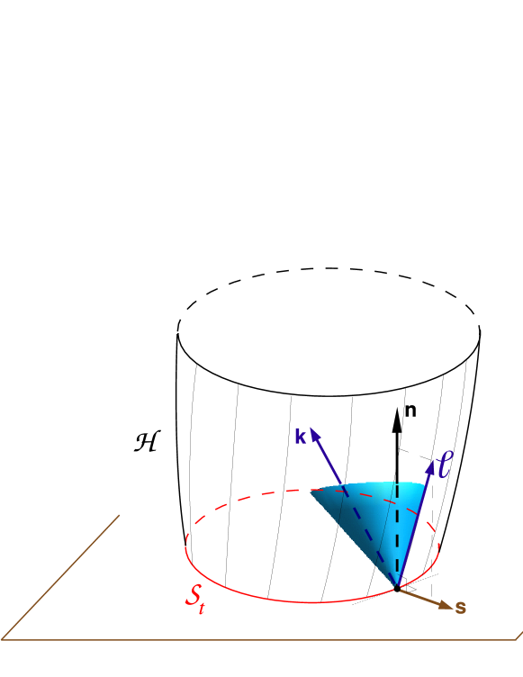
Figure 4.3: Null vector $\bm{\ell}$ normal to ${\mathcal{H}}$, unit timelike vector $\bm{n}$ normal to $\Sigma_{t}$, unit spacelike vector $\bm{s}$ normal to ${\mathcal{S}}_{t}$ and ingoing null vector $\bm{k}$ normal to ${\mathcal{S}}_{t}$.

Remark 4.1

Since $\bm{n}$ is a unit timelike vector, $\bm{s}$ a unit spacelike vector and they are orthogonal, it is immediate that the vector $\bm{n}+\bm{s}$ is null. The relation (4.13) implies that this vector is tangent to ${\mathcal{H}}$. Therefore, another natural normalization of the null normal to ${\mathcal{H}}$ would have been to consider $\bm{\ell}=\bm{n}+\bm{s}$, instead of $\langle\bm{\mathrm{d}}t,\bm{\ell}\rangle=1$ [Eq. (4.6)]. Both normalizations are induced by the foliation $(\Sigma_{t})$. Only the normalization (4.6) has the property of Lie dragging the surfaces $({\mathcal{S}}_{t})$. On the other side, at a given point $p\in{\mathcal{H}}$, the normalization $\bm{\ell}=\bm{n}+\bm{s}$ can be defined by a single spacelike hypersurface $\Sigma$ intersecting ${\mathcal{H}}$, whereas the normalization (4.6) requires the existence of a family $(\Sigma_{t})$ in the neighborhood of $p$. In what follows, we will denote by $\bm{\hat{\ell}}$ the null vector

$$\bm{\hat{\ell}}:=\frac{1}{\sqrt{2}}(\bm{n}+\bm{s}),$$ (4.14)

where the factor $1/\sqrt{2}$ is introduced for later convenience.

4.3 Unit spatial normal to ${\mathcal{S}}_{t}$

Equation (4.13) can be inverted to express the unit spatial normal to the surface ${\mathcal{S}}_{t}$, $\bm{s}$, in terms of $\bm{\ell}$ and $\bm{n}$:

$$\bm{s}=\frac{1}{N}\,\bm{\ell}-\bm{n}.$$ (4.15)

When combined with $\underline{\bm{\ell}}=\e^{\rho}\bm{\mathrm{d}}u$ [Eq. (2.14)] and $\underline{\bm{n}}=-N\,\bm{\mathrm{d}}t$ [Eq. (3.1)] this leads to the following expression of the 1-form $\underline{\bm{s}}$ associated with the normal $\bm{s}$:

$$\framebox{$\displaystyle\underline{\bm{s}}=N\bm{\mathrm{d}}t+M\bm{\mathrm{d}}u$},$$ (4.16)

where we have introduced the factor

$$M:=\frac{\e^{\rho}}{N},\qquad\mbox{so that}\quad\framebox{$\displaystyle\rho=\ln(MN)$}.$$ (4.17)

Equation (4.16) implies [cf. the definition (3.5) of the operator $\vec{\bm{\gamma}}^{*}$]

$$\vec{\bm{\gamma}}^{*}\underline{\bm{s}}=M\vec{\bm{\gamma}}^{*}\bm{\mathrm{d}}u,$$ (4.18)

because $\vec{\bm{\gamma}}^{*}\bm{\mathrm{d}}t=-N^{-1}\;\vec{\bm{\gamma}}^{*}\underline{\bm{n}}=0$. Now, since $\bm{s}\in{\mathcal{T}}_{p}(\Sigma_{t})$, $\vec{\bm{\gamma}}^{*}\underline{\bm{s}}=\underline{\bm{s}}$. Moreover, from Eq. (3.9), $\vec{\bm{\gamma}}^{*}\bm{\mathrm{d}}u=\bm{D}u$, so that we get

$$\framebox{$\displaystyle\underline{\bm{s}}=M\vec{\bm{\gamma}}^{*}\bm{\mathrm{d}}u=M\bm{D}u$}.$$ (4.19)

4.4 Induced metric on ${\mathcal{S}}_{t}$

The metric $\bm{h}$ induced by $\Sigma_{t}$’s metric $\bm{\gamma}$ on the 2-surfaces ${\mathcal{S}}_{t}$ is given by a formula analogous to Eq. (3.3), except for the change of the $+$ sign into a $-$ one, to take into account the spacelike character of the normal $\bm{s}$ (whereas the normal $\bm{n}$ was timelike):

$$\bm{h}:=\bm{\gamma}-\underline{\bm{s}}\otimes\underline{\bm{s}}=\bm{g}+\underline{\bm{n}}\otimes\underline{\bm{n}}-\underline{\bm{s}}\otimes\underline{\bm{s}}.$$ (4.20)

Let us consider a pair of vectors $(\bm{u},\bm{v})$ in ${\mathcal{T}}_{p}({\mathcal{H}})$. Denoting by $\bm{u}_{0}$ and $\bm{v}_{0}$ their respective projections along $\bm{\ell}$ on the vector plane ${\mathcal{T}}_{p}({\mathcal{S}}_{t})$, we have the unique decompositions

$$\bm{u}=\bm{u}_{0}+\lambda\bm{\ell}\quad\mbox{and}\quad\bm{v}=\bm{v}_{0}+\mu\bm{\ell},$$ (4.21)

where $\lambda$ and $\mu$ are two real numbers. Since $\bm{n}\cdot\bm{u}_{0}=\bm{n}\cdot\bm{v}_{0}=\bm{s}\cdot\bm{u}_{0}=\bm{s}\cdot\bm{v}_{0}=0$, one has

$$\bm{h}(\bm{u},\bm{v}) = \bm{g}(\bm{u},\bm{v})+\langle\underline{\bm{n}},\bm{u}\rangle\langle\underline{\bm{n}},\bm{v}\rangle-\langle\underline{\bm{s}},\bm{u}\rangle\langle\underline{\bm{s}},\bm{v}\rangle$$

$$= \bm{g}(\bm{u},\bm{v})+[\bm{n}\cdot(\bm{u}_{0}+\lambda\bm{\ell})]\times[\bm{n}\cdot(\bm{v}_{0}+\mu\bm{\ell})]-[\bm{s}\cdot(\bm{u}_{0}+\lambda\bm{\ell})]\times$$

$$[\bm{s}\cdot(\bm{v}_{0}+\mu\bm{\ell})]$$

$$= \bm{g}(\bm{u},\bm{v})+\lambda\mu(\underbrace{\bm{n}\cdot\bm{\ell}}_{=-N})^{2}-\lambda\mu(\underbrace{\bm{s}\cdot\bm{\ell}}_{=N})^{2}$$

$$\bm{h}(\bm{u},\bm{v}) = \bm{g}(\bm{u},\bm{v}).$$ (4.22)

This last equality shows that $\bm{h}$ and $\bm{g}$ coincide on ${\mathcal{T}}_{p}({\mathcal{H}})$. In other words, the pull-back of $\bm{h}$ on ${\mathcal{H}}$ equals the pull-back of $\bm{g}$, that we have denoted $\bm{q}$ in Sec. 2 [see Eq. (2.8)]: $\Phi^{*}\bm{h}=\Phi^{*}\bm{g}=\bm{q}$. We may then take $\bm{h}$ as the 4-dimensional extension of $\bm{q}$ and write Eq. (4.20) as

$$\framebox{$\displaystyle\bm{q}=\bm{\gamma}-\underline{\bm{s}}\otimes\underline{\bm{s}}$}$$ (4.23)

$$\framebox{$\displaystyle\bm{q}=\bm{g}+\underline{\bm{n}}\otimes\underline{\bm{n}}-\underline{\bm{s}}\otimes\underline{\bm{s}}$}.$$ (4.24)

Consequently we abandon from now on the notation $\bm{h}$ in profit of $\bm{q}$. To summarize, on ${\mathcal{T}}_{p}({\mathcal{M}})$, $\bm{q}$ is the symmetric bilinear form given by Eq. (4.24), on ${\mathcal{T}}_{p}(\Sigma_{t})$ it is the symmetric bilinear form given by Eq. (4.23), on ${\mathcal{T}}_{p}({\mathcal{H}})$ it is the degenerate metric induced by $\bm{g}$, and on ${\mathcal{T}}_{p}({\mathcal{S}}_{t})$ it is the positive definite (i.e. Riemannian) metric induced by $\bm{g}$.

The endomorphism ${\mathcal{T}}_{p}({\mathcal{M}})\rightarrow{\mathcal{T}}_{p}({\mathcal{M}})$ canonically associated with the bilinear form $\bm{q}$ by the metric $\bm{g}$ [cf. notation (1.12)] is the orthogonal projector onto the 2-surface ${\mathcal{S}}_{t}$:

$$\framebox{$\displaystyle\vec{\bm{q}}=\bm{1}+\bm{n}\,\langle\underline{\bm{n}},.\rangle-\bm{s}\,\langle\underline{\bm{s}},.\rangle$},$$ (4.25)

in the very same manner in which $\vec{\bm{\gamma}}$ defined by Eq. (3.4) was the orthogonal projector onto $\Sigma_{t}$.

4.5 Ingoing null vector

As mentioned in Sec. 4.1, we need some direction transverse to ${\mathcal{H}}$ to define a projector ${\mathcal{T}}_{p}({\mathcal{M}})\rightarrow{\mathcal{T}}_{p}({\mathcal{H}})$. The $(\Sigma_{t})$ slicing has already provided us with two different transverse directions: the timelike direction $\bm{n}$ and the spacelike direction $\bm{s}$, both normal to the 2-surfaces ${\mathcal{S}}_{t}$ (cf. Fig. 4.3). These two directions are indeed transverse to ${\mathcal{H}}$ since $\bm{n}\not\in{\mathcal{T}}_{p}({\mathcal{H}})$ (otherwise ${\mathcal{H}}$ would be a timelike hypersurface) and $\bm{s}\not\in{\mathcal{T}}_{p}({\mathcal{H}})$ (otherwise ${\mathcal{H}}$ would be a spacelike hypersurface, coinciding locally with $\Sigma_{t}$). However $\bm{n}$ and $\bm{s}$ are not the only natural choices linked with the $(\Sigma_{t})$ foliation: we may also think about the null directions normal to ${\mathcal{S}}_{t}$, i.e. the trajectories of the light rays emitted in the radial directions from points on ${\mathcal{S}}_{t}$. The light rays emitted in the outgoing radial direction (as defined in Sec. 4.2) define the null vector $\bm{\ell}$ tangent to ${\mathcal{H}}$ already introduced. But those emitted in the ingoing radial direction define (up to some normalization factor) another null vector:

$$\bm{\hat{k}}:=\frac{1}{\sqrt{2}}(\bm{n}-\bm{s})$$ (4.26)

[compare with Eq. (4.14)]. $\bm{\hat{k}}$ is transverse to ${\mathcal{H}}$, since $\bm{\ell}\cdot\bm{\hat{k}}=-\sqrt{2}N\not=0$. In fact we will favor this transverse direction, rather than those arising from $\bm{n}$ or $\bm{s}$, because its null character leads to simpler formulæ for the description of the null hypersurface ${\mathcal{H}}$.

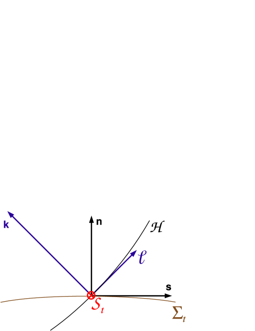
Figure 4.4: View of the plane orthogonal to the 2-surface ${\mathcal{S}}_{t}$: the timelike vector $\bm{n}$, the spacelike vector $\bm{s}$ and the null vectors $\bm{\ell}$ and $\bm{k}$ all belong to this plane. The dyad $(\bm{\ell},\bm{k})$ defines the intersection of this plane with the light cone emerging from ${\mathcal{S}}_{t}$’s points. Intersections of the hypersurfaces ${\mathcal{H}}$ and $\Sigma_{t}$ with this plane are also shown.

Let us renormalize the vector $\bm{\hat{k}}$ by dividing it by $\sqrt{2}N$ to get the null vector

$$\framebox{$\displaystyle\bm{k}={1\over 2N}(\bm{n}-\bm{s})$}.$$ (4.27)

The normalization has been chosen so that $\bm{k}$ satisfies the relation

$$\framebox{$\displaystyle\bm{\ell}\cdot\bm{k}=-1$},$$ (4.28)

which will simplify some of the subsequent formulæ. Equations (4.13) and (4.27) can be inverted to express $\bm{n}$ and $\bm{s}$ in terms of the null vectors $\bm{\ell}$ and $\bm{k}$:

$$\bm{n} = {1\over 2N}\,\bm{\ell}+N\,\bm{k}$$ (4.29)

$$\bm{s} = {1\over 2N}\,\bm{\ell}-N\,\bm{k}.$$ (4.30)

Each pair $(\bm{n},\bm{s})$ or $(\bm{\ell},\bm{k})$ forms a basis of the vectorial plane orthogonal to ${\mathcal{S}}_{t}$:

$${\mathcal{T}}_{p}({\mathcal{S}}_{t})^{\perp}={\rm Span}(\bm{n},\bm{s})={\rm Span}(\bm{\ell},\bm{k}).$$ (4.31)

This plane is shown in Fig. 4.4.

Remark 4.2

All the null vectors at a given point $p\in{\mathcal{H}}$, except those collinear to $\bm{\ell}$ are transverse to ${\mathcal{H}}$ (see Fig. 4.3 where all these vectors form the light cone emerging from $p$). It is the slicing $({\mathcal{S}}_{t})$ of ${\mathcal{H}}$ which has enabled us to select a preferred transverse null direction $\bm{k}$, as the unique null direction normal to ${\mathcal{S}}_{t}$ and different from $\bm{\ell}$.

Let us consider the 1-form $\underline{\bm{k}}$ canonically associated with the vector $\bm{k}$ by the metric $\bm{g}$. By combining Eqs. (4.27), (3.1) and (4.16), one gets

$$\framebox{$\displaystyle\underline{\bm{k}}=-\bm{\mathrm{d}}t-{M\over 2N}\bm{\mathrm{d}}u$}.$$ (4.32)

Remark 4.3

Equations (2.14), (3.1), (4.16) and (4.32) show that the 1-forms $\underline{\bm{\ell}}$, $\underline{\bm{n}}$, $\underline{\bm{s}}$ and $\underline{\bm{k}}$ are all linear combinations of the exact 1-forms $\bm{\mathrm{d}}t$ and $\bm{\mathrm{d}}u$. This simply reflects the fact that the vectors $\bm{\ell}$, $\bm{n}$, $\bm{s}$ and $\bm{k}$ are all orthogonal to ${\mathcal{S}}_{t}$ [Eq. (4.31) above] and that $(\bm{\mathrm{d}}t,\bm{\mathrm{d}}u)$ form a basis of the 2-dimensional space of 1-forms normal to ${\mathcal{S}}_{t}$ [see Eq. (4.4)].

An immediate consequence of (4.32) is that the action of $\underline{\bm{k}}$ on vectors tangent to ${\mathcal{H}}$ is identical (up to some sign) to the action of the gradient 1-form $\bm{\mathrm{d}}t$:

$$\forall\bm{v}\in{\mathcal{T}}_{p}({\mathcal{H}}),\quad\langle\underline{\bm{k}},\bm{v}\rangle=-\langle\bm{\mathrm{d}}t,\bm{v}\rangle.$$ (4.33)

An equivalent phrasing of this is: the pull-back of the 1-form $\underline{\bm{k}}$ on ${\mathcal{H}}$ and that of $-\bm{\mathrm{d}}t$ coincide:

$$\framebox{$\displaystyle\Phi^{*}\underline{\bm{k}}=-\Phi^{*}\bm{\mathrm{d}}t$}.$$ (4.34)

Remark 4.4

The null vector $\bm{k}$ can be seen as “dual” to the null vector $\bm{\ell}$ in the following sense: (i) $\bm{\ell}$ belongs to ${\mathcal{T}}_{p}({\mathcal{H}})$, while $\bm{k}$ does not, and (ii) $\Phi^{*}\underline{\bm{k}}$ is a non-trivial exact 1-form in ${\mathcal{T}}^{*}({\mathcal{H}})$, while $\Phi^{*}\underline{\bm{\ell}}$ is zero.

Example 4.5

Slicing of Minkowski light cone.
In continuation with Example 2.4 (${\mathcal{H}}$ = light cone in Minkowski spacetime), the simplest 3+1 slicing we may imagine is that constituted by hypersurfaces $t={\rm const}$, where $t$ is a standard Minkowskian time coordinate. The lapse function $N$ is then identically one and the unit normal to $\Sigma_{t}$ has trivial components with respect to the Minkowskian coordinates $(t,x,y,z)$: $n^{\alpha}=(1,0,0,0)$ and $n_{\alpha}=(-1,0,0,0)$. In Example 2.4, we have already normalized $\bm{\ell}$ so that $\ell^{t}=\langle\bm{\mathrm{d}}t,\bm{\ell}\rangle=1$ [Eq. (4.6)], [cf. Eq. (2.28)]. The 2-surface ${\mathcal{S}}_{t}$ is the sphere $r:=\sqrt{x^{2}+y^{2}+z^{2}}=t$ in the hyperplane $\Sigma_{t}$ and its outward unit normal has the following components with respect to $(t,x,y,z)$:

$$s^{\alpha}=\left(0,\frac{x}{r},\frac{y}{r},\frac{z}{r}\right),\quad s_{\alpha}=\left(0,\frac{x}{r},\frac{y}{r},\frac{z}{r}\right).$$ (4.35)

We then deduce the components of the ingoing null vector $\bm{k}$ from Eq. (4.27):

$$k^{\alpha}=\left(\frac{1}{2},-\frac{x}{2r},-\frac{y}{2r},-\frac{z}{2r}\right),\quad k_{\alpha}=\left(-\frac{1}{2},-\frac{x}{2r},-\frac{y}{2r},-\frac{z}{2r}\right),$$ (4.36)

and the components of $\bm{q}$ from Eq. (4.24):

$$q_{\alpha\beta}=\left(\begin{array}[]{cccc}0&0&0&0\\ 0&\frac{y^{2}+z^{2}}{r^{2}}&-\frac{xy}{r^{2}}&-\frac{xz}{r^{2}}\\ 0&-\frac{xy}{r^{2}}&\frac{x^{2}+z^{2}}{r^{2}}&-\frac{yz}{r^{2}}\\ 0&-\frac{xz}{r^{2}}&-\frac{yz}{r^{2}}&\frac{x^{2}+y^{2}}{r^{2}}\end{array}\right).$$ (4.37)

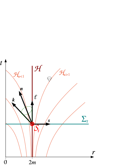
Figure 4.5: Null vector $\bm{\ell}$ normal to ${\mathcal{H}}$, unit timelike vector $\bm{n}$ normal to $\Sigma_{t}$, unit spacelike vector $\bm{s}$ normal to ${\mathcal{S}}_{t}$ and ingoing null vector $\bm{k}$ normal to ${\mathcal{S}}_{t}$ for the 3+1 Eddington-Finkelstein slicing of Schwarzschild horizon.

Example 4.6

Eddington-Finkelstein slicing of Schwarzschild horizon.
As a next example, let us consider the 3+1 slicing of Schwarzschild spacetime by the hypersurfaces $t={\rm const}$, where $t$ is the Eddington-Finkelstein time coordinate considered in Example 2.5. This slicing has been already represented in Fig. 2.4. The corresponding lapse function has been exhibited in Example 3.1. In Example 2.5, we have already normalized the null vector $\bm{\ell}$ to ensure $\ell^{t}=\langle\bm{\mathrm{d}}t,\bm{\ell}\rangle=1$, so Eq. (2.40) provides the correct expression for the null normal induced by the 3+1 slicing. From the metric components given by Eq. (2.34), we obtain immediately the expression of the unit normal to ${\mathcal{S}}_{t}$ lying in $\Sigma_{t}$:

$$s^{\alpha}=\left(0,\frac{1}{\sqrt{1+\frac{2m}{r}}},0,0\right),\quad s_{\alpha}=\left(\frac{2m}{r\sqrt{1+\frac{2m}{r}}},\sqrt{1+\frac{2m}{r}},0,0\right).$$ (4.38)

Inserting this value into formula (4.27) and making use of expression (3.26) for $N$ and (3.28) for $\bm{n}$, we get the ingoing null vector $\bm{k}$:

$$k^{\alpha}=\left(\frac{1}{2}+\frac{m}{r},-\frac{1}{2}-\frac{m}{r},0,0\right),\quad k_{\alpha}=\left(-\frac{1}{2}-\frac{m}{r},-\frac{1}{2}-\frac{m}{r},0,0\right).$$ (4.39)

Note that on ${\mathcal{H}}$, $k_{\alpha}\stackrel{{\scriptstyle{\mathcal{H}}}}{{=}}(-1,-1,0,0)$, so that we verify property (4.34), which is equivalent to $(k_{t},k_{\theta},k_{\varphi})\stackrel{{\scriptstyle{\mathcal{H}}}}{{=}}(-1,0,0)$. The vectors $\bm{n}$, $\bm{s}$, $\bm{\ell}$ and $\bm{k}$ are represented in Fig. 4.5. The 2-surface ${\mathcal{S}}_{t}$ is spanned by the coordinates $(\theta,\varphi)$ and the expression of the induced metric on ${\mathcal{S}}_{t}$ is obtained readily from the line element (2.34):

$$q_{\alpha\beta}={\rm diag}(0,0,r^{2},r^{2}\sin^{2}\theta).$$ (4.40)

4.6 Newman-Penrose null tetrad

4.6.1 Definition

The two null vectors $\bm{\ell}$ and $\bm{k}$ are the first two pieces of the so-called Newman-Penrose null tetrad, which we briefly present here. We complete the null pair $(\bm{\ell},\bm{k})$ by two orthonormal vectors in ${\mathcal{T}}_{p}({\mathcal{S}}_{t})$, $(\bm{e}_{a})=(\bm{e}_{2},\bm{e}_{3})$ let’s say, to get a basis of ${\mathcal{T}}_{p}({\mathcal{M}})$, such that

$$\begin{array}[]{lll}\bm{\ell}\cdot\bm{\ell}=0&\bm{\ell}\cdot\bm{k}=-1&\bm{\ell}\cdot\bm{e}_{a}=0\\ &\bm{k}\cdot\bm{k}=0&\bm{k}\cdot\bm{e}_{a}=0\\ &&\bm{e}_{a}\cdot\bm{e}_{b}=\delta_{ab}.\end{array}$$ (4.41)

The basis $(\bm{\ell},\bm{k},\bm{e}_{2},\bm{e}_{3})$ is formed by two null vectors and two spacelike vectors. At the price of introducing complex vectors, we can modify it into a basis of four null vectors. Indeed let us introduce the following combination of $\bm{e}_{2}$ and $\bm{e}_{3}$ with complex coefficients:

$$\bm{m}:={1\over\sqrt{2}}\left(\bm{e}_{2}+i\bm{e}_{3}\right).$$ (4.42)

Then the complex conjugate defines another vector, which is linearly independent from $\bm{m}$:

$$\bm{\bar{m}}={1\over\sqrt{2}}\left(\bm{e}_{2}-i\bm{e}_{3}\right).$$ (4.43)

Both $\bm{m}$ and $\bm{\bar{m}}$ are null vectors (with respect to the metric $\bm{g}$).

The tetrad $(\bm{\ell},\bm{k},\bm{m},\bm{\bar{m}})$ constitutes a basis of ${\mathcal{T}}_{p}({\mathcal{M}})$ made of null vectors only: any vector of ${\mathcal{T}}_{p}({\mathcal{M}})$ admits a unique expression as a linear combination (possibly with complex coefficients) of these four vectors. $(\bm{\ell},\bm{k},\bm{m},\bm{\bar{m}})$ is called a Newman-Penrose null tetrad [127] (see also p. 343 of Ref. [90] or p. 72 of [156]). This tetrad obeys to

$$\begin{array}[]{llll}\bm{\ell}\cdot\bm{\ell}=0&\bm{\ell}\cdot\bm{k}=-1&\bm{\ell}\cdot\bm{m}=0&\bm{\ell}\cdot\bm{\bar{m}}=0\\ &\bm{k}\cdot\bm{k}=0&\bm{k}\cdot\bm{m}=0&\bm{k}\cdot\bm{\bar{m}}=0\\ &&\bm{m}\cdot\bm{m}=0&\bm{m}\cdot\bm{\bar{m}}=1\\ &&&\bm{\bar{m}}\cdot\bm{\bar{m}}=0.\end{array}$$ (4.44)

Since $(\bm{e}_{2},\bm{e}_{3})$ is an orthonormal basis of ${\mathcal{T}}_{p}({\mathcal{S}}_{t})$, the metric induced in ${\mathcal{S}}_{t}$ can be written

$$\bm{q}=\underline{\bm{e}}_{2}\otimes\underline{\bm{e}}_{2}+\underline{\bm{e}}_{3}\otimes\underline{\bm{e}}_{3}=\underline{\bm{m}}\otimes\underline{\bm{\bar{m}}}+\underline{\bm{\bar{m}}}\otimes\underline{\bm{m}}.$$ (4.45)

Moreover $(\bm{n},\bm{s},\bm{e}_{2},\bm{e}_{3})$ is an orthonormal tetrad of ${\mathcal{T}}_{p}({\mathcal{M}})$. The spacetime metric can then be written

$$\bm{g}=-\underline{\bm{n}}\otimes\underline{\bm{n}}+\underline{\bm{s}}\otimes\underline{\bm{s}}+\underline{\bm{e}}_{2}\otimes\underline{\bm{e}}_{2}+\underline{\bm{e}}_{3}\otimes\underline{\bm{e}}_{3}.$$ (4.46)

It can also be expressed in terms of the Newman-Penrose null tetrad:

$$\bm{g}=-\underline{\bm{\ell}}\otimes\underline{\bm{k}}-\underline{\bm{k}}\otimes\underline{\bm{\ell}}+\underline{\bm{m}}\otimes\underline{\bm{\bar{m}}}+\underline{\bm{\bar{m}}}\otimes\underline{\bm{m}}.$$ (4.47)

Comparing Eqs. (4.47) and (4.45), we get an expression of $\bm{q}$ in terms of $\bm{g}$ and the null dyad $(\bm{\ell},\bm{k})$:

$$\framebox{$\displaystyle\bm{q}=\bm{g}+\underline{\bm{\ell}}\otimes\underline{\bm{k}}+\underline{\bm{k}}\otimes\underline{\bm{\ell}}$}.$$ (4.48)

This expression is alternative to Eq. (4.24). It can be obtained directly by inserting Eqs. (4.29) and (4.30) in Eq. (4.24). The related expression for the orthogonal projector $\vec{\bm{q}}$ onto the 2-surface ${\mathcal{S}}_{t}$ is

$$\framebox{$\displaystyle\vec{\bm{q}}=\bm{1}+\bm{\ell}\,\langle\underline{\bm{k}},.\rangle+\bm{k}\,\langle\underline{\bm{\ell}},.\rangle$},$$ (4.49)

which constitutes an alternative to Eq. (4.25).

4.6.2 Weyl scalars

In Section 1.2.2 we have introduced the Weyl tensor $\bm{C}$ and have indicated that it encodes ten of the twenty independent components of the Riemann tensor. The null tetrad previously introduced permits to write these free components as five independent complex scalars $\Psi_{n}$ ($n\in\{0,1,2,3,4\}$), known as Weyl scalars. They are defined as

$$\Psi_{0} := \bm{C}(\underline{\bm{\ell}},\bm{m},\bm{\ell},\bm{m})=C^{\mu}_{\ \,\nu\rho\sigma}\;\ell_{\mu}m^{\nu}\ell^{\rho}m^{\sigma}$$

$$\Psi_{1} := \bm{C}(\underline{\bm{\ell}},\bm{m},\bm{\ell},\bm{k})=C^{\mu}_{\ \,\nu\rho\sigma}\;\ell_{\mu}m^{\nu}\ell^{\rho}k^{\sigma}$$

$$\Psi_{2} := \bm{C}(\underline{\bm{\ell}},\bm{m},\bm{\bar{m}},\bm{k})=C^{\mu}_{\ \,\nu\rho\sigma}\;\ell_{\mu}m^{\nu}\bar{m}^{\rho}k^{\sigma}$$ (4.50)

$$\Psi_{3} := \bm{C}(\underline{\bm{\ell}},\bm{k},\bm{\bar{m}},\bm{k})=C^{\mu}_{\ \,\nu\rho\sigma}\;\ell_{\mu}k^{\nu}\bar{m}^{\rho}k^{\sigma}$$

$$\Psi_{4} := \bm{C}(\underline{\bm{\bar{m}}},\bm{k},\bm{\bar{m}},\bm{k})=C^{\mu}_{\ \,\nu\rho\sigma}\;\bar{m}_{\mu}k^{\nu}\bar{m}^{\rho}k^{\sigma}.$$

As we will see in the following sections, some relevant geometrical quantities are naturally expressed in terms of (some of) these scalars. For an account of the Newman-Penrose formalism in which they are naturally defined, see [155, 154, 45, 156] and references therein.

4.7 Projector onto ${\mathcal{H}}$

Having introduced the transverse null direction $\bm{k}$, we can now define the projector onto ${\mathcal{H}}$ along $\bm{k}$ by

$$\framebox{$\displaystyle\begin{array}[]{cccc}\bm{\Pi}:&{\mathcal{T}}_{p}({\mathcal{M}})&\longrightarrow&{\mathcal{T}}_{p}({\mathcal{H}})\\ &\bm{v}&\longmapsto&\bm{v}+(\bm{\ell}\cdot\bm{v})\,\bm{k}\end{array}$}$$ (4.51)

This application is well defined, i.e. its image is in ${\mathcal{T}}_{p}({\mathcal{H}})$, since

$$\forall\bm{v}\in{\mathcal{T}}_{p}({\mathcal{M}}),\quad\bm{\ell}\cdot\bm{\Pi}(\bm{v})=\bm{\ell}\cdot\bm{v}+(\bm{\ell}\cdot\bm{v})\,\underbrace{(\bm{\ell}\cdot\bm{k})}_{=-1}=0$$ (4.52)

Moreover, $\bm{\Pi}$ leaves invariant any vector in ${\mathcal{T}}_{p}({\mathcal{H}})$ :

$$\forall\bm{v}\in{\mathcal{T}}_{p}({\mathcal{H}}),\quad\bm{\Pi}(\bm{v})=\bm{v}$$ (4.53)

and

$$\bm{\Pi}(\bm{k})=0.$$ (4.54)

These last two properties show that the operator $\bm{\Pi}$ is the projector onto ${\mathcal{H}}$ along $\bm{k}$. The projector $\bm{\Pi}$ can be written as

$$\bm{\Pi}=\bm{1}+\bm{k}\,\langle\underline{\bm{\ell}},.\rangle.$$ (4.55)

It can be considered as a type $\left({1\atop 1}\right)$ tensor, whose components are

$$\Pi^{\alpha}_{\ \beta}=\delta^{\alpha}_{\ \beta}+k^{\alpha}\ell_{\beta}.$$ (4.56)

Comparing Eqs. (4.55) and (4.49) leads to the following relation

$$\vec{\bm{q}}=\bm{\Pi}+\bm{\ell}\,\langle\underline{\bm{k}},.\rangle.$$ (4.57)

Remark 4.7

The definition of the projector $\bm{\Pi}$ does not depend on the normalization of $\bm{\ell}$ and $\bm{k}$ as long as they satisfy the relation $\bm{\ell}\cdot\bm{k}=-1$ [Eq. (4.28)]. Indeed a rescaling $\bm{\ell}\mapsto\bm{\ell^{\prime}}=\alpha\bm{\ell}$ would imply a rescaling $\bm{k}\mapsto\bm{k^{\prime}}=\alpha^{-1}\bm{k}$, leaving $\bm{\Pi}$ invariant. In other words, $\bm{\Pi}$ is determined only by the foliation ${\mathcal{S}}_{t}$ of ${\mathcal{H}}$ and not by the scale of ${\mathcal{H}}$’s null normal. Note that such a foliation-induced tranverse projector onto a null hypersurface has been already used in the literature (see e.g. Ref. [30]).

Figure 4.6: Mappings between the space ${\mathcal{T}}_{p}({\mathcal{H}})$ (resp. ${\mathcal{T}}_{p}({\mathcal{M}})$) of vectors tangent to ${\mathcal{H}}$ (resp. ${\mathcal{M}}$) and the space ${\mathcal{T}}_{p}^{*}({\mathcal{H}})$ (resp. ${\mathcal{T}}_{p}^{*}({\mathcal{M}})$) of 1-forms on ${\mathcal{H}}$ (resp. ${\mathcal{M}}$): $\Phi_{*}$ and $\Phi^{*}$ are respectively the push-forward and the pull-back mapping canonically induced by the embedding of ${\mathcal{H}}$ in ${\mathcal{M}}$; $\bm{\Pi}$ is the projector onto ${\mathcal{H}}$ along the null transverse direction $\bm{k}$ and $\bm{\Pi}^{*}$ the induced mapping of 1-forms; $\bm{g}$ and $\bm{g}^{-1}$ denote the standard duality between vectors and 1-forms induced by the spacetime metric $\bm{g}$. Note that since the metric $\bm{q}$ on ${\mathcal{H}}$ is degenerate, it provides a mapping ${\mathcal{T}}_{p}({\mathcal{H}})\rightarrow{\mathcal{T}}_{p}^{*}({\mathcal{H}})$, but not in the reverse way. $\bm{\chi}$ is the Weingarten map, defined in Sec. 2.6, which is an endomorphism of ${\mathcal{T}}_{p}({\mathcal{H}})$.

Since $\bm{\Pi}$ is a well defined application ${\mathcal{T}}_{p}({\mathcal{M}})\rightarrow{\mathcal{T}}_{p}({\mathcal{H}})$, we may use it to map any linear form in ${\mathcal{T}}_{p}^{*}({\mathcal{H}})$ to a linear form in ${\mathcal{T}}_{p}^{*}({\mathcal{M}})$, in the very same way that in Sec. 2.1 we used the application $\Phi_{*}:\ {\mathcal{T}}_{p}({\mathcal{H}})\rightarrow{\mathcal{T}}_{p}({\mathcal{M}})$ to map linear forms in the opposite way, i.e. from ${\mathcal{T}}_{p}^{*}({\mathcal{M}})$ to ${\mathcal{T}}_{p}^{*}({\mathcal{H}})$. Indeed, and more generally, if $\bm{T}$ is a $n$-linear form on ${\mathcal{T}}_{p}({\mathcal{H}})^{n}$, we define $\bm{\Pi}^{*}\bm{T}$ as the $n$-linear form

$$\framebox{$\displaystyle\begin{array}[]{cccc}\bm{\Pi}^{*}\bm{T}:&{\mathcal{T}}_{p}({\mathcal{M}})^{n}&\longrightarrow&\mathbb{R}\\ &(\bm{v}_{1},\ldots,\bm{v}_{n})&\longmapsto&\bm{T}\left(\bm{\Pi}(\bm{v}_{1}),\ldots,\bm{\Pi}(\bm{v}_{n})\right)\end{array}$}.$$ (4.58)

Note that since any multilinear form on ${\mathcal{T}}_{p}({\mathcal{M}})^{n}$ can also be regarded as a multilinear form on ${\mathcal{T}}_{p}({\mathcal{H}})^{n}$ thanks to the pull-back mapping $\Phi^{*}$ if we identify $\Phi^{*}\bm{T}$ with $\bm{T}$ abusing of the notation [cf. Eq. (2.7)], we may extend the definition (4.58) to any multilinear form $\bm{T}$ on ${\mathcal{T}}_{p}({\mathcal{M}})$. In index notation, we have then

$$(\Pi^{*}T)_{\alpha_{1}\ldots\alpha_{n}}=T_{\mu_{1}\ldots\mu_{n}}\Pi^{\mu_{1}}_{\ \ \ \alpha_{1}}\cdots\Pi^{\mu_{n}}_{\ \ \ \alpha_{n}}.$$ (4.59)

Note that we are again abusing of the notation, since $\bm{\Pi}^{*}$ here should be properly denoted as $(\bm{\Pi}^{*}\circ\Phi^{*})\,\bm{T}$. In particular, for a 1-form, the expression (4.55) for $\bm{\Pi}$ yields:

$$\forall\bm{\varpi}\in{\mathcal{T}}_{p}^{*}({\mathcal{M}}),\quad\bm{\Pi}^{*}\bm{\varpi}=\bm{\varpi}+\langle\bm{\varpi},\bm{k}\rangle\,\underline{\bm{\ell}}.$$ (4.60)

For $\bm{\varpi}=\underline{\bm{\ell}}$, we get immediately

$$\bm{\Pi}^{*}\underline{\bm{\ell}}=0,$$ (4.61)

which reflects the fact that $\underline{\bm{\ell}}$ restricted to ${\mathcal{T}}_{p}({\mathcal{H}})$ vanishes. On the contrary, for the 1-form $\underline{\bm{k}}$ we have

$$\bm{\Pi}^{*}\underline{\bm{k}}=\underline{\bm{k}}.$$ (4.62)

Collecting together Eqs. (4.53) (for $\bm{v}=\bm{\ell}$), (4.54), (4.61) and (4.62), we recover the duality between $\bm{\ell}$ and $\bm{k}$ mentioned in Remark 4.4:

$$\framebox{$\displaystyle\bm{\Pi}(\bm{\ell})=\bm{\ell}$}\quad\mbox{and}\quad\framebox{$\displaystyle\bm{\Pi}(\bm{k})=0$},$$ (4.63)

$$\framebox{$\displaystyle\bm{\Pi}^{*}\underline{\bm{\ell}}=0$}\quad\mbox{and}\quad\framebox{$\displaystyle\bm{\Pi}^{*}\underline{\bm{k}}=\underline{\bm{k}}$}.$$ (4.64)

In index notation, the above relations write respectively

$$\Pi^{\alpha}_{\ \,\mu}\ell^{\mu}=\ell^{\alpha}\quad\mbox{and}\quad\Pi^{\alpha}_{\ \,\mu}k^{\mu}=0,$$ (4.65)

$$\ell_{\mu}\Pi^{\mu}_{\ \,\alpha}=0\quad\mbox{and}\quad k_{\mu}\Pi^{\mu}_{\ \,\alpha}=k_{\alpha}.$$ (4.66)

The various mappings introduced so far between the vectorial spaces ${\mathcal{T}}_{p}({\mathcal{H}})$ and ${\mathcal{T}}_{p}({\mathcal{M}})$ and their duals are represented in Fig. 4.6.

Remark 4.8

The vector $\bm{k}$ is a special case of what is called more generally a rigging vector [118], i.e. a vector transverse to ${\mathcal{H}}$ everywhere, which allows to define a projector onto ${\mathcal{H}}$ whatever the character of ${\mathcal{H}}$ (i.e. spacelike, timelike, null or changing from point to point).

4.8 Coordinate systems stationary with respect to ${\mathcal{H}}$

Let us consider a 3+1 coordinate system $(x^{\alpha})=(t,x^{i})$, with the associated coordinate time vector $\bm{t}$ and shift vector $\bm{\beta}$, as defined in Sec. 3.4. It is useful to perform an orthogonal 2+1 decomposition of the shift vector with respect to the surface ${\mathcal{S}}_{t}$, according to

$$\framebox{$\displaystyle\bm{\beta}=b\bm{s}-\bm{V}$}\qquad\mbox{with}\quad\bm{s}\cdot\bm{V}=0.$$ (4.67)

In other words, $b=\bm{s}\cdot\bm{\beta}$ and $\bm{V}=-\vec{\bm{q}}(\bm{\beta})\in{\mathcal{T}}_{p}({\mathcal{S}}_{t})$ (the minus sign is chosen for later convenience).

Combining the two 3+1 decompositions $\bm{\ell}=N(\bm{n}+\bm{s})$ [Eq. (4.13)] and $\bm{t}=N\bm{n}+\bm{\beta}$ [Eq. (3.24)], we get

$$\framebox{$\displaystyle\bm{\ell}=\bm{t}+\bm{V}+(N-b)\bm{s}$}.$$ (4.68)

We say that $(x^{\alpha})$ is a coordinate system stationary with respect to the null hypersurface ${\mathcal{H}}$ iff the equation of ${\mathcal{H}}$ in this coordinate system involves only the spatial coordinates $(x^{i})$ and does not depend upon $t$, i.e. iff there exist a scalar function $f(x^{1},x^{2},x^{3})$ such that

$$\forall\;p=(t,x^{1},x^{2},x^{3})\in{\mathcal{M}},\quad p\in{\mathcal{H}}\iff f(x^{1},x^{2},x^{3})=1.$$ (4.69)

This means that the location of the 2-surface ${\mathcal{S}}_{t}$ is fixed with respect to the coordinate system $(x^{i})$ on $\Sigma_{t}$, as $t$ varies. The gradient of $f$ is normal to ${\mathcal{H}}$ and thus parallel to $\bm{\mathrm{d}}u$:

$$\bm{\mathrm{d}}u\stackrel{{\scriptstyle{\mathcal{H}}}}{{=}}\alpha\,\bm{\mathrm{d}}f,$$ (4.70)

where $\stackrel{{\scriptstyle{\mathcal{H}}}}{{=}}$ means that this identity is valid only at points on ${\mathcal{H}}$ and $\alpha$ is some scalar field on ${\mathcal{H}}$. Equation (4.70) and the independence of $f$ from $t$ imply

$$\frac{\partial u}{\partial t}\stackrel{{\scriptstyle{\mathcal{H}}}}{{=}}0.$$ (4.71)

This has an immediate consequence on the coordinate time vector $\bm{t}$:

$$\langle\bm{\mathrm{d}}u,\bm{t}\rangle=\frac{\partial u}{\partial x^{\mu}}t^{\mu}=\frac{\partial u}{\partial x^{\mu}}\delta^{\mu}_{\ \,t}=\frac{\partial u}{\partial t}\stackrel{{\scriptstyle{\mathcal{H}}}}{{=}}0,$$ (4.72)

which implies that $\bm{t}$ is tangent to ${\mathcal{H}}$ [cf. Eq. (2.12)]. Consequently, for a coordinate system stationary with respect to ${\mathcal{H}}$,

$$\hat{\bm{\ell}}\cdot\bm{t}=0.$$ (4.73)

Replacing $\hat{\bm{\ell}}$ and $\bm{t}$ by their respective 3+1 decompositions (4.14) and (3.24) and using $b=\bm{s}\cdot\bm{\beta}$ leads to

$$b=N.$$ (4.74)

Thus, for a coordinate system stationary with respect to ${\mathcal{H}}$, the decomposition (4.68) simplifies to

$$\bm{\ell}=\bm{t}+\bm{V}.$$ (4.75)

In the case where ${\mathcal{H}}$ is the event horizon of some black hole and $(x^{\alpha})$ is stationary with respect to ${\mathcal{H}}$, $\bm{V}\in{\mathcal{T}}_{p}({\mathcal{S}}_{t})$ is called the surface velocity of the black hole by Damour [59, 60]. More generally, we will call $\bm{V}$ the surface velocity of ${\mathcal{H}}$ with respect to the coordinate system $(x^{\alpha})$ stationary with respect to ${\mathcal{H}}$.

To summarize, we have the following :

( $$(x^{\alpha}) {\mathcal{H}} \iff \frac{\partial u}{\partial t}\stackrel{{\scriptstyle{\mathcal{H}}}}{{=}}0$$ stationary w.r.t.  ) (4.76)

$$\iff \bm{t}\in{\mathcal{T}}_{p}({\mathcal{H}})$$ (4.77)

$$\iff \hat{\bm{\ell}}\cdot\bm{t}\stackrel{{\scriptstyle{\mathcal{H}}}}{{=}}0$$ (4.78)

$$\iff b\stackrel{{\scriptstyle{\mathcal{H}}}}{{=}}N$$ (4.79)

$$\iff \bm{\ell}\stackrel{{\scriptstyle{\mathcal{H}}}}{{=}}\bm{t}+\bm{V}$$ (4.80)

Notice that for a coordinate system stationary with respect to ${\mathcal{H}}$, the scalar field $u$ defining ${\mathcal{H}}$ is not necessarily such that $u=u(x^{1},x^{2},x^{3})$ everywhere in ${\mathcal{M}}$, but only on ${\mathcal{H}}$ [Eq. (4.76)].

The vectors $\bm{t}$, $\bm{\beta}$ and $\bm{V}$ of a coordinate system stationary with respect to ${\mathcal{H}}$ are shown in Fig. 4.7.

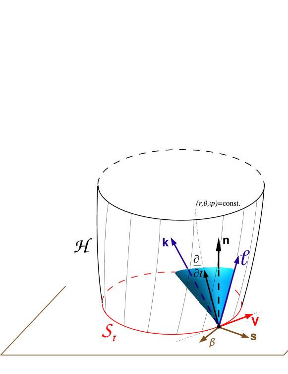
Figure 4.7: Same as Fig. 4.3 but with the addition of the coordinate time vector $\bm{t}$, the shift vector $\bm{\beta}$ and ${\mathcal{H}}$’s surface velocity vector $\bm{V}$ with respect to a coordinate system $(x^{\alpha})$ stationary with respect to ${\mathcal{H}}$.

A special case of a coordinate system stationary with respect to ${\mathcal{H}}$ is a coordinate system $(x^{\alpha})$ for which the function $f$ in Eq. (4.69) is simply one of the coordinates, $x^{1}$ let’s say: $f(x^{1},x^{2},x^{3})=x^{1}$. We call such a system a coordinate system adapted to ${\mathcal{H}}$. For instance, if the topology of ${\mathcal{H}}$ is $\mathbb{R}\times\mathbb{S}^{2}$, an adapted coordinate system can be of spherical type $(x^{i})=(r,\vartheta,\varphi)$, where $r$ is such that ${\mathcal{H}}$ corresponds to $r=1$.

Another special case of coordinate system stationary with respect to ${\mathcal{H}}$ is a coordinate system $(x^{\alpha})$ for which $\bm{V}=0$ (in addition to the stationarity condition $\bm{t}\in{\mathcal{T}}_{p}({\mathcal{H}})$). We call such a system a coordinate system comoving with ${\mathcal{H}}$. From Eq. (4.80) this implies

$$\bm{t}\stackrel{{\scriptstyle{\mathcal{H}}}}{{=}}\bm{\ell},$$ (4.81)

which shows that the null generators of ${\mathcal{H}}$ are some lines $x^{i}={\rm const}$.

Example 4.9

The Minkowskian coordinates $(t,x,y,z)$ introduced in Examples 2.4 and 4.5 are not stationary with respect to the light cone ${\mathcal{H}}$. In particular, $\partial u/\partial t=-1\not=0$ and $N=1\ \not=\ b=0$ for these coordinates. On the contrary, the Eddington-Finkelstein coordinates $(t,r,\theta,\varphi)$ introduced in Examples 2.5, 3.1 and 4.6 are stationary with respect to the event horizon ${\mathcal{H}}$ of a Schwarzschild black hole. In particular, from the expression (2.37) for $u$, we notice that the requirement (4.76) is fulfilled, and from Eqs. (3.27) and (4.38), we get $b=2m/r\,(1+2m/r)^{-1/2}$ so that $b\stackrel{{\scriptstyle{\mathcal{H}}}}{{=}}N\stackrel{{\scriptstyle{\mathcal{H}}}}{{=}}1/\sqrt{2}$, in agreement with (4.79). Moreover, the Eddington-Finkelstein coordinates are both adapted to ${\mathcal{H}}$ and comoving with ${\mathcal{H}}$. Indeed, the equation for ${\mathcal{H}}$ can be defined by $r=2m$ (instead of $u=1$), which shows the adaptation, and we have already noticed that $\bm{t}\stackrel{{\scriptstyle{\mathcal{H}}}}{{=}}\bm{\ell}$ [Eq. (2.41)], which shows the comobility (this can also be seen from the shift vector which is colinear to $\bm{s}$, according to Eqs. (3.27) and (4.38), implying $\bm{V}=0$).

If $(x^{\alpha})$ is a coordinate system adapted to ${\mathcal{H}}$, then $(x^{A})=(t,x^{a})=(t,x^{2},x^{3})$ is a coordinate system for ${\mathcal{H}}$. In terms of it, the induced metric element on ${\mathcal{H}}$ is

$$\left.ds^{2}\right|_{{\mathcal{H}}}=q_{AB}\,dx^{A}\,dx^{B}=g_{tt}\,dt^{2}+2g_{ta}\,dt\,dx^{a}+g_{ab}\,dx^{a}\,dx^{b}.$$ (4.82)

Now, from Eqs. (4.68) and (4.80),

$$g_{tt}=\bm{t}\cdot\bm{t}=(\bm{\ell}-\bm{V})\cdot(\bm{\ell}-\bm{V})=\bm{V}\cdot\bm{V}=V_{a}V^{a}$$ (4.83)

and, from Eqs. (4.67) and (4.16),

$$g_{ta}=\beta_{a}=bs_{a}-V_{a}=-V_{a}.$$ (4.84)

Besides, $g_{ab}=q_{ab}$ [cf. Eq. (2.9)]. Thus the above line element can be written

$$\framebox{$\displaystyle\left.ds^{2}\right|_{{\mathcal{H}}}=q_{AB}\,dx^{A}\,dx^{B}=q_{ab}(dx^{a}-V^{a}dt)(dx^{b}-V^{b}dt)$}$$ (4.85)

This equation agrees with Eq. (I.50c) of Damour [60] (or Eq. (6) of Appendix of Ref. [61]).

Example 4.10

For the Eddington-Finkelstein coordinates $(t,r,\theta,\varphi)$ considered in Examples 2.5, 3.1, 4.6 and 4.9, $(x^{A})=(t,\theta,\varphi)$ constitutes a coordinate system for the event horizon ${\mathcal{H}}$. Taking into account that $r=2m$ on ${\mathcal{H}}$, we read from the line element (2.34) that

$$\left.ds^{2}\right|_{{\mathcal{H}}}=r^{2}(d\theta^{2}+\sin^{2}\theta d\varphi^{2}),$$ (4.86)

in agreement with Eq. (4.85), with, in addition $V^{a}=0$, since the Eddington-Finkelstein coordinates are comoving with ${\mathcal{H}}$.

5 Null geometry in 4-dimensional version. Kinematics

In this section we consider the spacetime first derivatives of the null vectors $\bm{\ell}$ and $\bm{k}$ and of the associated 1-forms $\underline{\bm{\ell}}$ and $\underline{\bm{k}}$, as well as the Lie derivatives of the induced metric $\bm{q}$ along $\bm{\ell}$ and $\bm{k}$. This is what we mean by “kinematics”. The first derivative of $\bm{\ell}$ has been represented by the Weingarten map of ${\mathcal{H}}$ in Sec. 2.6. We start by extending the definition of this map to the whole 4-dimensional vector space ${\mathcal{T}}_{p}({\mathcal{M}})$, whereas its original definition was restricted to the 3-dimensional subspace ${\mathcal{T}}_{p}({\mathcal{H}})$.

5.1 4-dimensional extensions of the Weingarten map and the second fundamental form of ${\mathcal{H}}$

Having introduced in Sec. 4.7 the projector $\bm{\Pi}$ onto ${\mathcal{H}}$, we can extend the definition of the Weingarten map of ${\mathcal{H}}$ (with respect to the null normal $\bm{\ell}$) to all vectors of ${\mathcal{T}}_{p}({\mathcal{M}})$ at any point of ${\mathcal{H}}$, by setting

$$\framebox{$\displaystyle\begin{array}[]{cccc}\bm{\chi}:&{\mathcal{T}}_{p}({\mathcal{M}})&\longrightarrow&{\mathcal{T}}_{p}({\mathcal{H}})\\ &\bm{v}&\longmapsto&\bm{\chi}_{{\mathcal{H}}}(\bm{\Pi}(\bm{v}))\end{array}$},$$ (5.1)

where $\bm{\chi}_{{\mathcal{H}}}$ denotes the Weingarten map introduced on ${\mathcal{T}}_{p}({\mathcal{H}})$ in Sec. 2.6. The image of $\bm{\chi}$ is in ${\mathcal{T}}_{p}({\mathcal{H}})$ because the image of $\bm{\chi}_{{\mathcal{H}}}$ is. Explicitly, one has [cf. Eq. (2.50)]

$$\forall\bm{v}\in{\mathcal{T}}_{p}({\mathcal{M}}),\quad\bm{\chi}(\bm{v})=\bm{\nabla}_{\bm{\Pi}(\bm{v})}\,\bm{\ell}.$$ (5.2)

In index notation

$$\chi^{\alpha}_{\ \mu}v^{\mu}=\Pi(v)^{\nu}\nabla_{\nu}\ell^{\alpha}=(\delta^{\nu}_{\ \mu}+k^{\nu}\ell_{\mu})v^{\mu}\nabla_{\nu}\ell^{\alpha},$$ (5.3)

hence the matrix of $\bm{\chi}$:

$$\framebox{$\displaystyle\chi^{\alpha}_{\ \beta}=\nabla_{\beta}\ell^{\alpha}+k^{\mu}\nabla_{\mu}\ell^{\alpha}\,\ell_{\beta}$}.$$ (5.4)

We have already noticed that $\bm{\ell}$ is an eigenvector of the Weingarten map, with the eigenvalue $\kappa$ (the non-affinity coefficient) [cf. Eq. (2.56)]. Since $\bm{\Pi}(\bm{k})=0$, $\bm{k}$ constitutes another eigenvector of the (extended) Weingarten map, with the eigenvalue zero:

$$\framebox{$\displaystyle\bm{\chi}(\bm{\ell})=\kappa\,\bm{\ell}$}\qquad\mbox{and}\qquad\framebox{$\displaystyle\bm{\chi}(\bm{k})=0$}.$$ (5.5)

Similarly, we make use of the projector $\bm{\Pi}$ to extend the definition of the second fundamental form of ${\mathcal{H}}$ with respect to the normal $\bm{\ell}$ by [cf. the definition (4.58) of $\bm{\Pi}^{*}$]

$$\framebox{$\displaystyle\bm{\Theta}:=\bm{\Pi}^{*}\bm{\Theta}_{{\mathcal{H}}}$},$$ (5.6)

where $\bm{\Theta}_{{\mathcal{H}}}$ denotes the second fundamental form of ${\mathcal{H}}$ with respect to $\bm{\ell}$ introduced in Sec. 2.7. Explicitly, $\bm{\Theta}$ writes

$$\begin{array}[]{cccc}\bm{\Theta}:&{\mathcal{T}}_{p}({\mathcal{M}})\times{\mathcal{T}}_{p}({\mathcal{M}})&\longrightarrow&\mathbb{R}\\ &(\bm{u},\bm{v})&\longmapsto&\bm{\Theta}_{{\mathcal{H}}}\left(\bm{\Pi}(\bm{u}),\bm{\Pi}(\bm{v})\right).\end{array}$$ (5.7)

Since $\bm{\Theta}_{{\mathcal{H}}}$ is symmetric, the bilinear form $\bm{\Theta}$ defined above is symmetric. Moreover, from the relation (4.57), we have $\bm{\Pi}(\bm{u})=\vec{\bm{q}}(\bm{u})-\langle\underline{\bm{k}},\bm{u}\rangle\,\bm{\ell}$. Since $\bm{\ell}$ is a degeneracy direction of $\bm{\Theta}_{{\mathcal{H}}}$ [cf. Eq. (2.60)], we get

$$\forall(\bm{u},\bm{v})\in{\mathcal{T}}_{p}({\mathcal{M}})\times{\mathcal{T}}_{p}({\mathcal{M}}),\quad\bm{\Theta}(\bm{u},\bm{v})=\bm{\Theta}_{{\mathcal{H}}}(\vec{\bm{q}}(\bm{u}),\vec{\bm{q}}(\bm{v})).$$ (5.8)

Replacing $\bm{\Theta}_{{\mathcal{H}}}$ by its definition (2.57), we get

$$\forall(\bm{u},\bm{v})\in{\mathcal{T}}_{p}({\mathcal{M}})\times{\mathcal{T}}_{p}({\mathcal{M}}),\quad\bm{\Theta}(\bm{u},\bm{v}) = \vec{\bm{q}}(\bm{u})\cdot\bm{\nabla}_{\vec{\bm{q}}(\bm{v})}\,\bm{\ell}$$ (5.9)

$$= \bm{\nabla}\underline{\bm{\ell}}(\vec{\bm{q}}(\bm{u}),\vec{\bm{q}}(\bm{v})).$$

We write this relation as

$$\framebox{$\displaystyle\bm{\Theta}=\vec{\bm{q}}^{*}\,\bm{\nabla}\underline{\bm{\ell}}$},$$ (5.10)

where $\vec{\bm{q}}^{*}$ is the operator on multilinear forms induced by the projector $\vec{\bm{q}}$, in a manner similar to $\bm{\Pi}^{*}$ [cf. Eq. (4.58)]: for any $n$-linear form $\bm{T}$ on ${\mathcal{T}}_{p}({\mathcal{M}})$ or on ${\mathcal{T}}_{p}({\mathcal{S}}_{t})$, $\vec{\bm{q}}^{*}\,\bm{T}$ is the $n$-linear form on ${\mathcal{T}}_{p}({\mathcal{M}})$ defined by

$$\framebox{$\displaystyle\begin{array}[]{cccc}\vec{\bm{q}}^{*}\,\bm{T}:&{\mathcal{T}}_{p}({\mathcal{M}})^{n}&\longrightarrow&\mathbb{R}\\ &(\bm{v}_{1},\ldots,\bm{v}_{n})&\longmapsto&\bm{T}\left(\vec{\bm{q}}(\bm{v}_{1}),\ldots,\vec{\bm{q}}(\bm{v}_{n})\right)\end{array}$}.$$ (5.11)

In index notation:

$$(\vec{q}^{*}T)_{\alpha_{1}\ldots\alpha_{n}}=T_{\mu_{1}\ldots\mu_{n}}\,q^{\mu_{1}}_{\ \ \ \alpha_{1}}\cdots q^{\mu_{n}}_{\ \ \ \alpha_{n}},$$ (5.12)

so that Eq. (5.10) writes (taking into account the symmetry of $\bm{\Theta}$)

$$\framebox{$\displaystyle\Theta_{\alpha\beta}=\nabla_{\mu}\ell_{\nu}\;q^{\mu}_{\ \alpha}q^{\nu}_{\ \beta}$}.$$ (5.13)

The identity (5.10) strengthens Eq. (5.6): not only $\bm{\Theta}$ “acts only” in ${\mathcal{H}}$ (in the sense that $\bm{\Theta}$ starts by a projection onto ${\mathcal{H}}$), but it “acts only” in the submanifold ${\mathcal{S}}_{t}$ of ${\mathcal{H}}$.

The bilinear form $\bm{\Theta}$ is degenerate, with at least two degeneracy directions : $\bm{\ell}$ [see Eq. (2.60)] and $\bm{k}$ (since $\bm{\Pi}(\bm{k})=0$):

$$\framebox{$\displaystyle\bm{\Theta}(\bm{\ell},.)=0$}\qquad\mbox{and}\qquad\framebox{$\displaystyle\bm{\Theta}(\bm{k},.)=0$}.$$ (5.14)

From Eq. (4.31) we conclude that any vector in the plane orthogonal to ${\mathcal{S}}_{t}$ is also a degeneracy direction for $\bm{\Theta}$:

$$\forall\bm{v}\in{\mathcal{T}}_{p}({\mathcal{S}}_{t})^{\perp},\quad\bm{\Theta}(\bm{v},.)=0.$$ (5.15)

5.2 Expression of $\bm{\nabla}\bm{\ell}$: rotation 1-form and Háj́iček 1-form

A quantity which appears very often in our study is the spacetime covariant derivative of the null normal: $\bm{\nabla}\underline{\bm{\ell}}$. Let us recall that, thanks to some null foliation $({\mathcal{H}}_{u})$, we have extended the definition of $\bm{\ell}$ to an open neighborhood of ${\mathcal{H}}$ (cf. Sec. 2.3). Consequently the covariant derivatives $\bm{\nabla}\bm{\ell}$ and $\bm{\nabla}\underline{\bm{\ell}}$ are well defined. $\bm{\nabla}\underline{\bm{\ell}}$ is a bilinear form on ${\mathcal{T}}_{p}({\mathcal{M}})$. Let us express it in terms of the bilinear form $\bm{\Theta}$ which we have just extended to the whole space ${\mathcal{T}}_{p}({\mathcal{M}})$. For two arbitrary vectors $\bm{u}$ and $\bm{v}$ of ${\mathcal{T}}_{p}({\mathcal{M}})$, by combining the definition (5.7) of $\bm{\Theta}$ with the definition (2.57) of $\bm{\Theta}_{{\mathcal{H}}}$ and making use of the expression (4.51) of $\bm{\Pi}$, one has

$$\bm{\Theta}(\bm{u},\bm{v}) = \bm{\Pi}(\bm{u})\cdot\bm{\nabla}_{\bm{\Pi}(v)}\bm{\ell}\ =\ \left(\bm{u}+\langle\underline{\bm{\ell}},\bm{u}\rangle\bm{k}\right)\cdot\bm{\nabla}_{\bm{\Pi}(v)}\bm{\ell}$$ (5.16)

$$= \bm{u}\cdot\bm{\nabla}_{\bm{\Pi}(v)}\bm{\ell}+\langle\underline{\bm{\ell}},\bm{u}\rangle\bm{k}\cdot\underbrace{\bm{\nabla}_{\bm{\Pi}(v)}\bm{\ell}}_{=\bm{\chi}(\bm{v})}=\bm{u}\cdot\bm{\nabla}_{\bm{v}+\langle\underline{\bm{\ell}},\bm{v}\rangle\bm{k}}\bm{\ell}+\langle\underline{\bm{\ell}},\bm{u}\rangle\bm{k}\cdot\bm{\chi}(\bm{v})$$

$$= \bm{u}\cdot\bm{\nabla}_{\bm{v}}\bm{\ell}+\langle\underline{\bm{\ell}},\bm{v}\rangle\bm{u}\cdot\bm{\nabla}_{\bm{k}}\bm{\ell}+\langle\underline{\bm{\ell}},\bm{u}\rangle\bm{k}\cdot\bm{\chi}(\bm{v})$$

$$= \bm{\nabla}\underline{\bm{\ell}}(\bm{u},\bm{v})+\langle\underline{\bm{\ell}},\bm{v}\rangle\langle\bm{\nabla}_{\bm{k}}\,\underline{\bm{\ell}},\bm{u}\rangle+\langle\underline{\bm{\ell}},\bm{u}\rangle\bm{k}\cdot\bm{\chi}(\bm{v}).$$

In this expression appears the 1-form

$$\framebox{$\displaystyle\begin{array}[]{cccc}\bm{\omega}:&{\mathcal{T}}_{p}({\mathcal{M}})&\longrightarrow&\mathbb{R}\\ &\bm{v}&\longmapsto&-\bm{k}\cdot\bm{\chi}(\bm{v})\end{array}$},$$ (5.17)

which we call the rotation 1-form (for reasons which will become clear later; see Sec. 8.6.1). The relation (5.16) then reads

$$\bm{\Theta}(\bm{u},\bm{v})=\bm{\nabla}\underline{\bm{\ell}}(\bm{u},\bm{v})+\langle\underline{\bm{\ell}},\bm{v}\rangle\langle\bm{\nabla}_{\bm{k}}\,\underline{\bm{\ell}},\bm{u}\rangle-\langle\bm{\omega},\bm{v}\rangle\langle\underline{\bm{\ell}},\bm{u}\rangle.$$ (5.18)

Since this equation is valid whatever $\bm{u}$ and $\bm{v}$ in ${\mathcal{T}}_{p}({\mathcal{M}})$, we obtain the relation we were looking for:

$$\framebox{$\displaystyle\bm{\nabla}\underline{\bm{\ell}}=\bm{\Theta}+\underline{\bm{\ell}}\otimes\bm{\omega}-\bm{\nabla}_{\bm{k}}\,\underline{\bm{\ell}}\otimes\underline{\bm{\ell}}$}.$$ (5.19)

Taking into account the symmetry of $\bm{\Theta}$, the ‘index’ version of the above relation is [see Eq. (1.9)]:

$$\nabla_{\alpha}\ell_{\beta}=\Theta_{\alpha\beta}+\omega_{\alpha}\ell_{\beta}-\ell_{\alpha}k^{\mu}\nabla_{\mu}\ell_{\beta}.$$ (5.20)

An equivalent form of Eq. (5.19), obtained via the standard metric duality [or by raising the last index of Eq. (5.20)], gives the covariant derivative of the vector field $\bm{\ell}$

$$\bm{\nabla}\bm{\ell}=\vec{\bm{\Theta}}+\bm{\ell}\otimes\bm{\omega}-\bm{\nabla}_{\bm{k}}\,\bm{\ell}\otimes\underline{\bm{\ell}},$$ (5.21)

where $\vec{\bm{\Theta}}$ is the endomorphism canonically associated with the bilinear form $\bm{\Theta}$ by the metric $\bm{g}$ [see the notation (1.12)]. Its components are $\Theta^{\alpha}_{\ \,\beta}=g^{\alpha\mu}\Theta_{\mu\beta}$ and it is related to the Weingarten map $\bm{\chi}$ by

$$\vec{\bm{\Theta}}:=\vec{\bm{q}}\circ\bm{\chi}\circ\vec{\bm{q}}=\vec{\bm{q}}\circ\bm{\chi}.$$ (5.22)

By combining Eqs. (5.2), (5.21) and using the fact that $\langle\bm{\omega},\bm{k}\rangle=0$, so that $\langle\bm{\omega},\bm{\Pi}(\bm{v})\rangle=\langle\bm{\omega},\bm{v}\rangle$ for any $\bm{v}\in{\mathcal{T}}_{p}({\mathcal{M}})$, we get a simple expression relating the extended Weingarten map to the endomorphism $\vec{\bm{\Theta}}$ and the rotation 1-form $\bm{\omega}$:

$$\framebox{$\displaystyle\bm{\chi}=\vec{\bm{\Theta}}+\langle\bm{\omega},.\rangle\,\bm{\ell}$}.$$ (5.23)

Let us now discuss further the rotation 1-form $\bm{\omega}$. First, from the expressions (5.2) for $\bm{\chi}$ and (4.51) for $\bm{\Pi}$, one has

$$\forall\bm{v}\in{\mathcal{T}}_{p}({\mathcal{M}}),\quad\langle\bm{\omega},\bm{v}\rangle = -\bm{k}\cdot\bm{\nabla}_{\bm{\Pi}(\bm{v})}\,\bm{\ell}=-\bm{k}\cdot\bm{\nabla}_{\bm{v}+\langle\underline{\bm{\ell}},\bm{v}\rangle\bm{k}}\,\bm{\ell}$$ (5.24)

$$= -\bm{k}\cdot\bm{\nabla}_{\bm{v}}\,\bm{\ell}-\langle\underline{\bm{\ell}},\bm{v}\rangle\bm{k}\cdot\bm{\nabla}_{\bm{k}}\,\bm{\ell}.$$

Hence

$$\bm{\omega}=-\bm{k}\cdot\bm{\nabla}\underline{\bm{\ell}}-(\bm{k}\cdot\bm{\nabla}_{\bm{k}}\bm{\ell})\;\underline{\bm{\ell}}.$$ (5.25)

Next, for any vector $\bm{v}\in{\mathcal{T}}_{p}({\mathcal{M}})$ we have $\langle\bm{\omega},\bm{v}\rangle=-\langle\underline{\bm{k}},\bm{\chi}(\bm{v})\rangle$. Since the image of the extended Weingarten map $\bm{\chi}$ is in ${\mathcal{T}}_{p}({\mathcal{H}})$ and the action of the 1-forms $\underline{\bm{k}}$ and $-\bm{\mathrm{d}}t$ coincide on ${\mathcal{T}}_{p}({\mathcal{H}})$ [cf. Eq. (4.34)], we get the following alternative expressions for $\bm{\omega}$:

$$\forall\bm{v}\in{\mathcal{T}}_{p}({\mathcal{M}}),\quad\langle\bm{\omega},\bm{v}\rangle=\langle\bm{\mathrm{d}}t,\bm{\chi}(\bm{v})\rangle=\langle\bm{\mathrm{d}}t,\bm{\nabla}_{\bm{\Pi}(v)}\bm{\ell}\rangle,$$ (5.26)

which we can write in terms of the function composition operator $\circ$ as

$$\framebox{$\displaystyle\bm{\omega}=\bm{\mathrm{d}}t\;\circ\;\bm{\chi}$}.$$ (5.27)

Besides, from the very definition (5.17) of $\bm{\omega}$, the eigenvector expressions (5.5) lead immediately to the following action on the null vectors $\bm{\ell}$ and $\bm{k}$:

$$\framebox{$\displaystyle\langle\bm{\omega},\bm{\ell}\rangle=\kappa$}\qquad\mbox{and}\qquad\framebox{$\displaystyle\langle\bm{\omega},\bm{k}\rangle=0$}.$$ (5.28)

The pull-back of the rotation 1-form to the 2-surfaces ${\mathcal{S}}_{t}$ by the inclusion mapping of ${\mathcal{S}}_{t}$ into ${\mathcal{M}}$ is called the Háj́iček  1-form and is denoted by the capital letter $\bm{\Omega}$. Following the 4-dimensional point of view adopted in this article, we can extend the definition of $\bm{\Omega}$ to all vectors in ${\mathcal{T}}_{p}({\mathcal{M}})$ thanks to the orthogonal projector $\vec{\bm{q}}$ and set [see definition (5.11)]

$$\framebox{$\displaystyle\bm{\Omega}:=\bm{\omega}\,\circ\,\vec{\bm{q}}$}\qquad\mbox{or}\qquad\framebox{$\displaystyle\bm{\Omega}:=\vec{\bm{q}}^{*}\bm{\omega}$}.$$ (5.29)

Replacing $\bm{\omega}$ by its definition (5.17) leads to

$$\forall\bm{v}\in{\mathcal{T}}_{p}({\mathcal{M}}),\quad\framebox{$\displaystyle\langle\bm{\Omega},\bm{v}\rangle=-\bm{k}\cdot\bm{\nabla}_{\vec{\bm{q}}(\bm{v})}\,\bm{\ell}$}.$$ (5.30)

The 1-form $\bm{\Omega}$ has been introduced by Háj́iček [82, 84] in the special case $\bm{\Theta}=0$ (non-expanding horizons, to be discussed in Sec. 7) and in the general case by Damour [60, 61]. $\bm{\Omega}$ is considered by Háj́iček  as a “gravimagnetic field”, whereas it is viewed by Damour as a surface momentum density, as we shall see in Sec. 6.3. The form $\bm{\Omega}$ has also been used in the subsequent membrane paradigm formulation of Price & Thorne [141]. Actually, restricting the action of $\bm{\Omega}$ to ${\mathcal{T}}_{p}({\mathcal{S}}_{t})$, on which $\vec{\bm{q}}$ is the identity operator, and using Eq. (5.26), we get

$$\forall\bm{v}\in{\mathcal{T}}_{p}({\mathcal{S}}_{t}),\quad\langle\bm{\Omega},\bm{v}\rangle=\langle\bm{\mathrm{d}}t,\,\bm{\nabla}_{\bm{v}}\,\bm{\ell}\rangle,$$ (5.31)

This expression agrees with Eq. (2.6) of Ref. [141], used by Price & Thorne as the definition of the Háj́iček 1-form. By construction (because of the orthonormal projector $\vec{\bm{q}}$ onto ${\mathcal{S}}_{t}$), the Háj́iček 1-form vanishes for any vector orthogonal to the 2-surface ${\mathcal{S}}_{t}$:

$$\forall\bm{v}\in{\mathcal{T}}_{p}({\mathcal{S}}_{t})^{\perp},\quad\langle\bm{\Omega},\bm{v}\rangle=0.$$ (5.32)

In particular, it vanishes on the null dyad $(\bm{\ell},\bm{k})$:

$$\framebox{$\displaystyle\langle\bm{\Omega},\bm{\ell}\rangle=0$}\qquad\mbox{and}\qquad\framebox{$\displaystyle\langle\bm{\Omega},\bm{k}\rangle=0$}.$$ (5.33)

Actually the 1-form $\bm{\Omega}$ can be viewed as a 1-form intrinsic to the 2-surface ${\mathcal{S}}_{t}$, independently of the fact that ${\mathcal{S}}_{t}$ is a submanifold of ${\mathcal{H}}$ or $\Sigma_{t}$. It describes some part of the extrinsic geometry of ${\mathcal{S}}_{t}$ as a submanifold of $({\mathcal{M}},\bm{g})$ and is called generically a normal fundamental form of the 2-surface ${\mathcal{S}}_{t}$ [93, 67, 76]. The remaining part of the extrinsic geometry of ${\mathcal{S}}_{t}$ is described by the second fundamental tensor $\bm{\mathcal{K}}$ discussed in Remark 5.4 below.

We have, thanks to the expression (4.57) for $\vec{\bm{q}}$,

$$\forall\bm{v}\in{\mathcal{T}}_{p}({\mathcal{M}}),\quad\langle\bm{\Omega},\bm{v}\rangle = \langle\bm{\omega},\vec{\bm{q}}(\bm{v})\rangle=\langle\bm{\omega},\bm{\Pi}(\bm{v})+\langle\underline{\bm{k}},\bm{v}\rangle\,\bm{\ell}\rangle$$ (5.34)

$$= \underbrace{\langle\bm{\omega},\bm{\Pi}(\bm{v})\rangle}_{=\langle\bm{\omega},\bm{v}\rangle}+\langle\underline{\bm{k}},\bm{v}\rangle\underbrace{\langle\bm{\omega},\bm{\ell}\rangle}_{=\kappa}.$$

Hence it follows the simple relation between the rotation 1-form $\bm{\omega}$, the Háj́iček 1-form $\bm{\Omega}$ and the “transverse” 1-form $\underline{\bm{k}}$:

$$\framebox{$\displaystyle\bm{\omega}=\bm{\Omega}-\kappa\,\underline{\bm{k}}$}.$$ (5.35)

5.3 Frobenius identities

From the expression (5.19) of the spacetime covariant derivative $\bm{\nabla}\underline{\bm{\ell}}$, we can compute the exterior derivative of ${\mathcal{H}}$’s normal 1-form $\underline{\bm{\ell}}$ following Eq. (1.24). We get, taking into account the symmetry of $\bm{\Theta}$,

$$\bm{\mathrm{d}}\underline{\bm{\ell}} = \bm{\omega}\otimes\underline{\bm{\ell}}-\underline{\bm{\ell}}\otimes\bm{\omega}-\underline{\bm{\ell}}\otimes\bm{\nabla}_{\bm{k}}\,\underline{\bm{\ell}}+\bm{\nabla}_{\bm{k}}\,\underline{\bm{\ell}}\otimes\underline{\bm{\ell}}=\bm{\omega}\wedge\underline{\bm{\ell}}+\bm{\nabla}_{\bm{k}}\,\underline{\bm{\ell}}\wedge\underline{\bm{\ell}}$$

$$\bm{\mathrm{d}}\underline{\bm{\ell}} = \left(\bm{\omega}+\bm{\nabla}_{\bm{k}}\,\underline{\bm{\ell}}\right)\wedge\underline{\bm{\ell}}.$$ (5.36)

The fact that the exterior derivative of $\underline{\bm{\ell}}$ is the exterior product of some 1-form with $\underline{\bm{\ell}}$ itself reflects the fact that $\underline{\bm{\ell}}$ is normal to some hypersurface (${\mathcal{H}}$): this is the dual formulation of Frobenius theorem already noticed in Sec. 2.4. Actually Eq. (5.36) has the same structure as Eq. (2.17). Let us rewrite the latter by expressing $\rho$ is terms of the lapse function $N$ and the factor $M$ [Eq. (4.17)]:

$$\framebox{$\displaystyle\bm{\mathrm{d}}\underline{\bm{\ell}}=\bm{\mathrm{d}}\ln(MN)\wedge\underline{\bm{\ell}}$}.$$ (5.37)

Let us now evaluate the exterior derivative of the 1-form $\underline{\bm{k}}$ dual to the ingoing null vector $\bm{k}$. First of all, the definition of $\bm{k}$ is extended to an open neighborhood of ${\mathcal{H}}$ in ${\mathcal{M}}$ as the vector field which satisfies (i) $\bm{k}$ is an ingoing null normal to the 2-surface ${\mathcal{S}}_{t,u}$ [cf. Eq. (4.2)] and (ii) $\bm{k}\cdot\bm{\ell}=-1$. The exterior derivative $\bm{\mathrm{d}}\underline{\bm{k}}$ is then well defined. Starting from expression (4.32) for $\underline{\bm{k}}$ and using $\bm{\mathrm{d}}\bm{\mathrm{d}}=0$, we have immediately [cf. formula (1.22)]

$$\bm{\mathrm{d}}\underline{\bm{k}}=-\frac{1}{2}\;\bm{\mathrm{d}}\left(\frac{M}{N}\right)\wedge\bm{\mathrm{d}}u=-\frac{1}{2MN}\;\bm{\mathrm{d}}\left(\frac{M}{N}\right)\wedge\underline{\bm{\ell}},$$ (5.38)

where we have used $\underline{\bm{\ell}}=MN\bm{\mathrm{d}}u$ [cf. Eq. (2.14)]. Hence

$$\framebox{$\displaystyle\bm{\mathrm{d}}\underline{\bm{k}}=\frac{1}{2N^{2}}\;\bm{\mathrm{d}}\ln\left(\frac{N}{M}\right)\wedge\underline{\bm{\ell}}$}.$$ (5.39)

Remark 5.1

Since a priori the 1-form $\bm{\mathrm{d}}\ln(N/M)$ is not of the form $\alpha\underline{\bm{k}}+\beta\underline{\bm{\ell}}$ (in which case Eq. (5.39) would write $\bm{\mathrm{d}}\underline{\bm{k}}=\alpha/(2N^{2})\,\underline{\bm{k}}\wedge\underline{\bm{\ell}}$), we deduce from the (dual formulation of) of Frobenius theorem (see e.g. Theorem B.3.2 in Wald’s textbook [167]) and Eq. (5.39) that the hyperplane normal to $\underline{\bm{k}}$ is not integrable into some hypersurface. On the other side, the Frobenius theorem and relations (5.37) and (5.39) imply that the 2-planes normal to both $\underline{\bm{\ell}}$ and $\underline{\bm{k}}$ are integrable into a 2-surface: it is ${\mathcal{S}}_{t}$ [cf. the property (4.31)].

5.4 Another expression of the rotation 1-form

Let us show that the Frobenius identity (5.39) leads to the identification of the rotation 1-form $\bm{\omega}$ with the covariant derivative of the 1-form $\underline{\bm{k}}$ along the vector $\bm{\ell}$. Starting from the definition of $\bm{\omega}$ [Eq. (5.17)], any vector $\bm{v}\in{\mathcal{T}}_{p}({\mathcal{M}})$ satisfies

$$\langle\bm{\omega},\bm{v}\rangle = -\bm{k}\cdot\bm{\nabla}_{\bm{\Pi}(\bm{v})}\bm{\ell}=\bm{\ell}\cdot\bm{\nabla}_{\bm{\Pi}(\bm{v})}\bm{k}=\langle\bm{\nabla}_{\bm{\Pi}(\bm{v})}\underline{\bm{k}},\bm{\ell}\rangle=\langle\bm{\nabla}\underline{\bm{k}}\cdot\bm{\Pi}(\bm{v}),\;\bm{\ell}\rangle$$ (5.40)

$$= \langle-\bm{\mathrm{d}}\underline{\bm{k}}\cdot\bm{\Pi}(\bm{v})+\bm{\Pi}(\bm{v})\cdot\bm{\nabla}\underline{\bm{k}},\;\bm{\ell}\rangle$$

$$= \left\langle\frac{1}{2N^{2}}\left[\bm{\nabla}_{\bm{\Pi}(\bm{v})}\ln\left(\frac{N}{M}\right)\;\underline{\bm{\ell}}-\underbrace{\langle\underline{\bm{\ell}},\bm{\Pi}(\bm{v})\rangle}_{=0}\bm{\mathrm{d}}\ln\left(\frac{N}{M}\right)\right],\ \bm{\ell}\right\rangle$$

$$+\ \langle\bm{\Pi}(\bm{v})\cdot\bm{\nabla}\underline{\bm{k}},\;\bm{\ell}\rangle$$

$$= \frac{1}{2N^{2}}\bm{\nabla}_{\bm{\Pi}(\bm{v})}\ln\left(\frac{N}{M}\right)\;\underbrace{\langle\underline{\bm{\ell}},\bm{\ell}\rangle}_{=0}\ +\ \langle\bm{\nabla}_{\bm{\ell}}\underline{\bm{k}},\bm{\Pi}(\bm{v})\rangle$$

$$= \langle\bm{\nabla}_{\bm{\ell}}\,\underline{\bm{k}},\;\bm{v}+(\bm{\ell}\cdot\bm{v})\bm{k}\rangle=\langle\bm{\nabla}_{\bm{\ell}}\,\underline{\bm{k}},\bm{v}\rangle+(\bm{\ell}\cdot\bm{v})\underbrace{\langle\bm{\nabla}_{\bm{\ell}}\,\underline{\bm{k}},\bm{k}\rangle}_{=0}$$

$$= \langle\bm{\nabla}_{\bm{\ell}}\,\underline{\bm{k}},\bm{v}\rangle,$$

where the relation $\bm{k}\cdot\bm{\ell}=-1$ has been used in the first line, Eq. (1.24) to obtain the second line, and Eq. (5.39) to get the third line. Therefore

$$\framebox{$\displaystyle\bm{\omega}=\bm{\nabla}_{\bm{\ell}}\,\underline{\bm{k}}$}.$$ (5.41)

From Eq. (4.34), $\underline{\bm{k}}$ can be written as $\underline{\bm{k}}=-\bm{\Pi}^{*}\bm{\mathrm{d}}t$ on ${\mathcal{H}}$. If we make use of this, together with the expression (4.57) for $\bm{\Pi}$, the pull-back of the above relation on ${\mathcal{H}}$ results in

$$\framebox{$\displaystyle\Phi^{*}\bm{\omega}=-\Phi^{*}\bm{\nabla}_{\bm{\ell}}\,\bm{\mathrm{d}}t$},$$ (5.42)

which provides some nice perspective on $\bm{\omega}$, alternative to Eq. (5.27). Combining Eqs. (5.41) and (5.28) results in the simple relation

$$\bm{\nabla}\underline{\bm{k}}(\bm{\ell},\bm{\ell})=\kappa.$$ (5.43)

Another consequence of the Frobenius identity (5.39) is

$$\bm{k}\cdot\bm{\mathrm{d}}\underline{\bm{k}} = \frac{1}{2N^{2}}\left[\bm{\nabla}_{\bm{k}}\ln\left(\frac{N}{M}\right)\;\underline{\bm{\ell}}-\underbrace{\langle\underline{\bm{\ell}},\bm{k}\rangle}_{=-1}\bm{\mathrm{d}}\ln\left(\frac{N}{M}\right)\right]$$

$$\bm{\nabla}\underline{\bm{k}}\cdot\bm{k}-\underbrace{\bm{k}\cdot\bm{\nabla}\underline{\bm{k}}}_{=0} = \frac{1}{2N^{2}}\left[\bm{\nabla}_{\bm{k}}\ln\left(\frac{N}{M}\right)\;\underline{\bm{\ell}}+\bm{\mathrm{d}}\ln\left(\frac{N}{M}\right)\right].$$ (5.44)

Hence [cf. Eq. (4.60)]

$$\framebox{$\displaystyle\bm{\nabla}_{\bm{k}}\,\underline{\bm{k}}=\frac{1}{2N^{2}}\bm{\Pi}^{*}\bm{\mathrm{d}}\ln\left(\frac{N}{M}\right)$}.$$ (5.45)

Since $\bm{\nabla}\underline{\bm{\ell}}(\bm{k},\bm{k})=\bm{k}\cdot\bm{\nabla}_{\bm{k}}\,\bm{\ell}=-\bm{\ell}\cdot\bm{\nabla}_{\bm{k}}\,\bm{k}=-\langle\bm{\nabla}_{\bm{k}}\,\underline{\bm{k}},\bm{\ell}\rangle$ and $\bm{\Pi}(\bm{\ell})=\bm{\ell}$, we deduce from the above relation that

$$\bm{\nabla}\underline{\bm{\ell}}(\bm{k},\bm{k})=-\frac{1}{2N^{2}}\bm{\nabla}_{\bm{\ell}}\ln\left(\frac{N}{M}\right).$$ (5.46)

Let us now evaluate $\bm{\nabla}_{\bm{k}}\,\underline{\bm{\ell}}$. Contracting the Frobenius relation (5.37) for $\underline{\bm{\ell}}$ with the vector $\bm{k}$ yields

$$\bm{k}\cdot\bm{\mathrm{d}}\underline{\bm{\ell}} = \bm{\nabla}_{\bm{k}}\ln(MN)\;\underline{\bm{\ell}}-\underbrace{\langle\underline{\bm{\ell}},\bm{k}\rangle}_{=-1}\bm{\mathrm{d}}\ln(MN)$$

$$\bm{\nabla}\underline{\bm{\ell}}\cdot\bm{k}-\bm{k}\cdot\bm{\nabla}\underline{\bm{\ell}} = \bm{\Pi}^{*}\bm{\mathrm{d}}\ln(MN)$$

$$\bm{\nabla}_{\bm{k}}\,\underline{\bm{\ell}} = \bm{k}\cdot\bm{\nabla}\underline{\bm{\ell}}+\bm{\Pi}^{*}\bm{\mathrm{d}}\ln(MN)\ .$$ (5.47)

Substituting Eq. (5.25) for $\bm{k}\cdot\bm{\nabla}\underline{\bm{\ell}}$ and using Eq. (5.46) gives

$$\framebox{$\displaystyle\bm{\nabla}_{\bm{k}}\,\underline{\bm{\ell}}=-\bm{\omega}+\frac{1}{2N^{2}}\bm{\nabla}_{\bm{\ell}}\ln\left(\frac{N}{M}\right)\;\underline{\bm{\ell}}+\bm{\Pi}^{*}\bm{\mathrm{d}}\ln(MN)$}.$$ (5.48)

From this relation and Eqs. (5.46) and (4.60), we get the following expression for the rotation 1-form:

$$\bm{\omega}=\bm{\Pi}^{*}\left(\bm{\mathrm{d}}\ln(MN)-\bm{\nabla}_{\bm{k}}\,\underline{\bm{\ell}}\right),$$ (5.49)

which clearly shows that the action of $\bm{\omega}$ vanishes in the direction $\bm{k}$.

5.5 Deformation rate of the 2-surfaces ${\mathcal{S}}_{t}$

The choice of $\bm{\ell}$ as the tangent vector to ${\mathcal{H}}$’s null generators corresponding to the parameter $t$ (cf. Sec. 4.2) makes it the natural vector field to describe the evolution of ${\mathcal{H}}$’s fields with respect to $t$. Following Damour [60, 61], we define the tensor of deformation rate with respect to $\bm{\ell}$ of the 2-surface ${\mathcal{S}}_{t}$ as half the Lie derivative of ${\mathcal{S}}_{t}$’s metric $\bm{q}$ along the vector field $\bm{\ell}$:

$$\bm{Q}:=\frac{1}{2}\,{}^{{\mathcal{S}}}\!\bm{\mathcal{L}}_{\bm{\bm{\ell}}}\,\bm{q},$$ (5.50)

where $\bm{q}$ is considered as a bilinear form field on ${\mathcal{S}}_{t}$ and ${}^{{\mathcal{S}}}\!\bm{\mathcal{L}}_{\bm{\bm{\ell}}}\,$ is the Lie derivative intrinsic to $({\mathcal{S}}_{t})$ which arises from the Lie-dragging of ${\mathcal{S}}_{t}$ by $\bm{\ell}$ (cf. Sec. 4.2 and Fig. 4.2). The precise definition of ${}^{{\mathcal{S}}}\!\bm{\mathcal{L}}_{\bm{\bm{\ell}}}\,$ is given in Appendix A. The relation with the Lie derivative along $\bm{\ell}$ within the manifold ${\mathcal{M}}$, $\bm{\mathcal{L}}_{\bm{\bm{\ell}}}\,$, is given in 4-dimensional form by Eq. (A.20)

$$\vec{\bm{q}}^{*}{}^{{\mathcal{S}}}\!\bm{\mathcal{L}}_{\bm{\bm{\ell}}}\,\bm{q}=\vec{\bm{q}}^{*}\bm{\mathcal{L}}_{\bm{\bm{\ell}}}\,\bm{q},$$ (5.51)

where we have used $\vec{\bm{q}}^{*}\bm{q}=\bm{q}$. Thus Eq. (5.50) becomes

$$\vec{\bm{q}}^{*}\bm{Q}=\frac{1}{2}\vec{\bm{q}}^{*}\bm{\mathcal{L}}_{\bm{\bm{\ell}}}\,\bm{q},$$ (5.52)

where $\bm{q}$ is now considered as a bilinear form on ${\mathcal{M}}$ [as given by Eq. (4.24) or Eq. (4.48)]. Let us evaluate the (4-dimensional) Lie derivative in the right-hand side of the above equation, by substituting Eq. (4.48) for $\bm{q}$:

$$\bm{\mathcal{L}}_{\bm{\bm{\ell}}}\,\bm{q} = \bm{\mathcal{L}}_{\bm{\bm{\ell}}}\,(\bm{g}+\underline{\bm{\ell}}\otimes\underline{\bm{k}}+\underline{\bm{k}}\otimes\underline{\bm{\ell}})$$ (5.53)

$$= \bm{\mathcal{L}}_{\bm{\bm{\ell}}}\,\bm{g}+\bm{\mathcal{L}}_{\bm{\bm{\ell}}}\,\underline{\bm{\ell}}\otimes\underline{\bm{k}}+\underline{\bm{\ell}}\otimes\bm{\mathcal{L}}_{\bm{\bm{\ell}}}\,\underline{\bm{k}}+\bm{\mathcal{L}}_{\bm{\bm{\ell}}}\,\underline{\bm{k}}\otimes\underline{\bm{\ell}}+\underline{\bm{k}}\otimes\bm{\mathcal{L}}_{\bm{\bm{\ell}}}\,\underline{\bm{\ell}}.$$

Since $\vec{\bm{q}}^{*}\underline{\bm{\ell}}=0$ and $\vec{\bm{q}}^{*}\underline{\bm{k}}=0$, only the term $\bm{\mathcal{L}}_{\bm{\bm{\ell}}}\,\bm{g}$ remains in the right-hand side when applying the operator $\vec{\bm{q}}^{*}$, so that Eq. (5.52) becomes

$$\vec{\bm{q}}^{*}\bm{Q}=\frac{1}{2}\vec{\bm{q}}^{*}\bm{\mathcal{L}}_{\bm{\bm{\ell}}}\,\bm{g}.$$ (5.54)

Now $\bm{\mathcal{L}}_{\bm{\bm{\ell}}}\,\bm{g}$ is the Killing operator applied to the 1-form $\underline{\bm{\ell}}$ : ${\mathcal{L}}_{\bm{\bm{\ell}}}\,g_{\alpha\beta}=\nabla_{\alpha}\ell_{\beta}+\nabla_{\beta}\ell_{\alpha}$. Then from Eq. (5.13) and taking into account the symmetry of $\bm{\Theta}$, we get

$$\vec{\bm{q}}^{*}\bm{Q}=\bm{\Theta}.$$ (5.55)

Replacing $\bm{Q}$ by its definition (5.50), we conclude that the second fundamental form of ${\mathcal{H}}$ is related to the deformation rate of the 2-surface ${\mathcal{S}}_{t}$ by

$$\framebox{$\displaystyle\bm{\Theta}=\frac{1}{2}\,\vec{\bm{q}}^{*}\;{}^{{\mathcal{S}}}\!\bm{\mathcal{L}}_{\bm{\bm{\ell}}}\,\bm{q}=\frac{1}{2}\,\vec{\bm{q}}^{*}\;\bm{\mathcal{L}}_{\bm{\bm{\ell}}}\,\bm{q}$},$$ (5.56)

where the second equality follows from Eq. (5.51).

Let us consider a coordinate system $(x^{\alpha})=(t,x^{i})$. Then, according to Eq. (4.68), $\bm{\ell}=\bm{t}+\bm{V}+(N-b)\bm{s}$, where $\bm{t}$ is the coordinate time vector associated with $(x^{\alpha})$, $\bm{V}=\vec{\bm{q}}(\bm{\ell}-\bm{t})$, and $b$ is the component of the shift vector of $(x^{\alpha})$ along the spatial normal $\bm{s}$ to $\Sigma_{t}$. Equation (5.56) can then be written

$$\Theta_{\alpha\beta} = \frac{1}{2}\left({\mathcal{L}}_{\bm{\bm{t}}}\,q_{\mu\nu}+{\mathcal{L}}_{\bm{\bm{V}}}\,q_{\mu\nu}+{\mathcal{L}}_{(N-b)\bm{s}}\,q_{\mu\nu}\right)q^{\mu}_{\ \,\alpha}q^{\nu}_{\ \,\beta}$$

$$= \frac{1}{2}\Big{\{}{\mathcal{L}}_{\bm{\bm{t}}}\,q_{\mu\nu}+V^{\sigma}\nabla_{\sigma}q_{\mu\nu}+q_{\sigma\nu}\nabla_{\mu}V^{\sigma}+q_{\mu\sigma}\nabla_{\nu}V^{\sigma}+(N-b)s^{\sigma}\nabla_{\sigma}q_{\mu\nu}$$

$$+q_{\sigma\nu}\nabla_{\mu}[(N-b)s^{\sigma}]+q_{\mu\sigma}\nabla_{\nu}[(N-b)s^{\sigma}]\Big{\}}\,q^{\mu}_{\ \,\alpha}q^{\nu}_{\ \,\beta}$$

$$= \frac{1}{2}\Big{\{}\left({\mathcal{L}}_{\bm{\bm{t}}}\,q_{\mu\nu}\right)q^{\mu}_{\ \,\alpha}q^{\nu}_{\ \,\beta}+q^{\mu}_{\ \,\alpha}q_{\sigma\beta}\nabla_{\mu}V^{\sigma}+q_{\alpha\sigma}q^{\nu}_{\ \,\beta}\nabla_{\nu}V^{\sigma}$$

$$+(N-b)\left(q^{\mu}_{\ \,\alpha}q_{\sigma\beta}\nabla_{\mu}s^{\sigma}+q_{\alpha\sigma}q^{\nu}_{\ \,\beta}\nabla_{\nu}s^{\sigma}\right)\Big{\}}$$

$$\Theta_{\alpha\beta} = \frac{1}{2}\left[{\mathcal{L}}_{\bm{\bm{t}}}\,q_{\mu\nu}+\nabla_{\mu}V_{\nu}+\nabla_{\nu}V_{\mu}+(N-b)\left(\nabla_{\mu}s_{\nu}+\nabla_{\nu}s_{\mu}\right)\right]q^{\mu}_{\ \,\alpha}q^{\nu}_{\ \,\beta},$$ (5.57)

where the last but one equality results from the identities $q_{\mu\sigma}s^{\sigma}=0$ and $q^{\mu}_{\ \,\alpha}q^{\nu}_{\ \,\beta}\nabla_{\sigma}q_{\mu\nu}=0$. This last identity follows immediately from Eq. (4.48). Now, similarly to Eq. (3.8) and thanks to the fact that $\bm{V}\in{\mathcal{T}}({\mathcal{S}}_{t})$,

$$q^{\mu}_{\ \,\alpha}q^{\nu}_{\ \,\beta}\nabla_{\mu}V_{\nu}={}^{2}\!D_{\alpha}V_{\beta},$$ (5.58)

where $\bm{{}^{2}\!D}$ denotes the covariant derivative in the surface ${\mathcal{S}}_{t}$ compatible with the induced metric $\bm{q}$. More generally the relation between $\bm{{}^{2}\!D}$ derivatives and $\bm{\nabla}$ derivatives is given by a formula analogous to Eq. (3.8), with the projector $\vec{\bm{\gamma}}$ simply replaced by the projector $\vec{\bm{q}}$:

$$\framebox{$\displaystyle{}^{2}\!D_{\gamma}T^{\alpha_{1}\ldots\alpha_{p}}_{\ \qquad\beta_{1}\ldots\beta_{q}}=q_{\ \ \,\mu_{1}}^{\alpha_{1}}\,\cdots q_{\ \ \,\mu_{p}}^{\alpha_{p}}\,q_{\ \ \,\beta_{1}}^{\nu_{1}}\,\cdots q_{\ \ \,\beta_{q}}^{\nu_{q}}\,q_{\ \ \,\gamma}^{\sigma}\,\nabla_{\sigma}T^{\mu_{1}\ldots\mu_{p}}_{\ \qquad\nu_{1}\ldots\nu_{q}}$},$$ (5.59)

where $\bm{T}$ is any tensor of type $\left({p\atop q}\right)$ lying in ${\mathcal{S}}_{t}$ (i.e. such that its contraction with the normal vectors $\bm{n}$ and $\bm{s}$ (or $\bm{\ell}$ and $\bm{k}$) on any of its indices vanishes). On the other side

$$\left(\nabla_{\mu}s_{\nu}+\nabla_{\nu}s_{\mu}\right)q^{\mu}_{\ \,\alpha}q^{\nu}_{\ \,\beta}=H_{\beta\alpha}+H_{\alpha\beta}=2H_{\alpha\beta},$$ (5.60)

where $\bm{H}$ is the extrinsic curvature of the surface ${\mathcal{S}}_{t}$ considered as a hypersurface embedded in the Riemannian space $(\Sigma_{t},\bm{\gamma})$. $\bm{H}$ is a symmetric bilinear form which vanishes in the directions orthogonal to ${\mathcal{S}}_{t}$. It will be discussed in a greater extent in Sec. 10.3.1. In particular the formula (5.60) is a direct consequence of Eq. (10.32) established in that section.

Thanks to Eqs. (5.58) and (5.60), Eq. (5.57) becomes

$$\framebox{$\displaystyle\Theta_{\alpha\beta}=\frac{1}{2}\left[\left({\mathcal{L}}_{\bm{\bm{t}}}\,q_{\mu\nu}\right)q^{\mu}_{\ \,\alpha}q^{\nu}_{\ \,\beta}+{}^{2}\!D_{\alpha}V_{\beta}+{}^{2}\!D_{\beta}V_{\alpha}\right]+(N-b)H_{\alpha\beta}$},$$ (5.61)

or, in index-free notation (cf. the definition (1.27) of the Killing operator):

$$\framebox{$\displaystyle\bm{\Theta}=\frac{1}{2}\left[\vec{\bm{q}}^{*}\bm{\mathcal{L}}_{\bm{\bm{t}}}\,\bm{q}+\,{\rm Kil}(\bm{{}^{2}\!D},\underline{\bm{V}})\right]+(N-b)\bm{H}$}.$$ (5.62)

In particular, if $(x^{\alpha})$ is a coordinate system adapted to ${\mathcal{H}}$, then $N-b=0$ [Eq. (4.79)] and $q^{\mu}_{\ \,a}=\delta^{\mu}_{\ \,a}$, so that when restricting Eq. (5.61) to ${\mathcal{S}}_{t}$ (i.e. $\alpha=a\in\{2,3\}$, $\beta=b\in\{2,3\}$) one obtains

$$\framebox{$\displaystyle\Theta_{ab}={1\over 2}\left(\frac{\partial q_{ab}}{\partial t}+{}^{2}\!D_{a}V_{b}+{}^{2}\!D_{b}V_{a}\right)$},$$ (5.63)

which agrees with Eq. (I.52b) of Damour [60].

5.6 Expansion scalar and shear tensor of the 2-surfaces ${\mathcal{S}}_{t}$

Let us split the second fundamental form $\bm{\Theta}$ (now considered as the deformation rate of the 2-surfaces ${\mathcal{S}}_{t}$) into a trace part and a traceless part with respect to ${\mathcal{S}}_{t}$’s metric $\bm{q}$

$$\framebox{$\displaystyle\bm{\Theta}=\frac{1}{2}\theta\,\bm{q}+\bm{\sigma}$},$$ (5.64)

where

$$\framebox{$\displaystyle\theta:=\,{\rm tr}\,\vec{\bm{\Theta}}=\Theta^{\mu}_{\ \ \mu}=g^{\mu\nu}\Theta_{\mu\nu}=q^{\mu\nu}\Theta_{\mu\nu}=q^{ab}\Theta_{ab}=\Theta^{a}_{\ \,a}$}$$ (5.65)

is the trace of the endomorphism $\vec{\bm{\Theta}}$ canonically associated with $\bm{\Theta}$ by the metric $\bm{g}$ [see also Eq. (5.22)] and $\bm{\sigma}$ is the traceless part of $\bm{\Theta}$

$$\bm{\sigma}:=\bm{\Theta}-\frac{1}{2}\theta\,\bm{q},$$ (5.66)

which satisfies

$$\sigma^{\mu}_{\ \ \mu}=q^{\mu\nu}\sigma_{\mu\nu}=\sigma^{a}_{\ \,a}=0.$$ (5.67)

The trace $\theta$ is called the expansion scalar of ${\mathcal{S}}_{t}$ and $\bm{\sigma}$ the shear tensor of ${\mathcal{S}}_{t}$.

The expansion $\theta$ is linked to the divergence of $\bm{\ell}$; indeed taking the trace of Eq. (5.21) results in

$$\bm{\nabla}\cdot\bm{\ell}=\theta+\underbrace{\langle\bm{\omega},\bm{\ell}\rangle}_{=\kappa}-\underbrace{\langle\underline{\bm{\ell}},\bm{\nabla}_{\bm{k}}\bm{\ell}\rangle}_{=0},$$ (5.68)

hence

$$\framebox{$\displaystyle\bm{\nabla}\cdot\bm{\ell}=\kappa+\theta$}.$$ (5.69)

Another relation is obtained by combining $\theta=q^{\mu\nu}\Theta_{\mu\nu}$ with the expression (5.9) for $\Theta_{\mu\nu}$:

$$\theta=q^{\mu\nu}q^{\rho}_{\ \ \mu}q^{\sigma}_{\ \ \nu}\nabla_{\rho}\ell_{\sigma}=q^{\nu\rho}q^{\sigma}_{\ \ \nu}\nabla_{\rho}\ell_{\sigma}=q^{\rho\sigma}\nabla_{\rho}\ell_{\sigma},$$ (5.70)

i.e.

$$\framebox{$\displaystyle\theta=q^{\mu\nu}\nabla_{\mu}\ell_{\nu}$}.$$ (5.71)

Another expression of $\theta$ is obtained as follows. Let $(x^{\alpha})$ be a coordinate system adapted to ${\mathcal{H}}$; $(x^{a})_{a=2,3}$ is then a coordinate system on ${\mathcal{S}}_{t}$. We have $\theta=q^{ab}\Theta_{ab}$ [cf. Eq. (5.65)] and let us use Eq. (5.56) restricted to ${\mathcal{T}}({\mathcal{S}}_{t})$, i.e. under the form $\Theta_{ab}=1/2\;{}^{{\mathcal{S}}}\!\bm{\mathcal{L}}_{\bm{\bm{\ell}}}\,q_{ab}$. We get

$$\theta=\frac{1}{2}\,q^{ab}\;{}^{{\mathcal{S}}}\!\bm{\mathcal{L}}_{\bm{\bm{\ell}}}\,q_{ab}=\frac{1}{2}\,{}^{{\mathcal{S}}}\!\bm{\mathcal{L}}_{\bm{\bm{\ell}}}\,\ln q,$$ (5.72)

where $q$ is the determinant of the components $q_{ab}$ of the metric $\bm{q}$ with respect to the coordinates $(x^{a})$ in ${\mathcal{S}}_{t}$:

$$\framebox{$\displaystyle q:=\det q_{ab}$}.$$ (5.73)

The second equality in Eq. (5.72) follows from the standard formula for the variation of a determinant. Hence we have

$$\framebox{$\displaystyle\theta={}^{{\mathcal{S}}}\!\bm{\mathcal{L}}_{\bm{\bm{\ell}}}\,\ln\sqrt{q}$}.$$ (5.74)

This relation justifies the name of expansion scalar given to $\theta$, for $\sqrt{q}$ is related to the surface element ${}^{2}\bm{\epsilon}$ of ${\mathcal{S}}_{t}$ by

$${}^{2}\bm{\epsilon}=\sqrt{q}\,\bm{\mathrm{d}}x^{2}\wedge\bm{\mathrm{d}}x^{3}.$$ (5.75)

Another expression of $\theta$ is obtained by contracting Eq. (5.63) with $q^{ab}$:

$$\framebox{$\displaystyle\theta=\frac{\partial}{\partial t}\ln\sqrt{q}+{}^{2}\!D_{a}V^{a}$}.$$ (5.76)

More generally, contracting Eq. (5.61) with $q^{\alpha\beta}$ leads to

$$\framebox{$\displaystyle\theta=q^{\mu\nu}{\mathcal{L}}_{\bm{\bm{t}}}\,q_{\mu\nu}+{}^{2}\!D_{a}V^{a}+(N-b)H$},$$ (5.77)

where $H$ is twice ${\mathcal{S}}_{t}$’s mean curvature within $(\Sigma_{t},\bm{\gamma})$ [Eq. (10.41) below].

Remark 5.2

Equations (5.74) and (5.76), by relating $\theta$ to the rate of expansion of the 2-surfaces ${\mathcal{S}}_{t}$, might suggest that the scalar $\theta$ depends quite sensitively upon the foliation of spacetime by the spacelike hypersurfaces $\Sigma_{t}$, since the surfaces ${\mathcal{S}}_{t}$ are defined by this foliation. Actually the dependence is pretty weak: as shown by Eq. (5.69), $\theta$ depends only upon the null normal $\bm{\ell}$ to ${\mathcal{H}}$ (since $\kappa$ depends only upon $\bm{\ell}$). Hence the dependence of $\theta$ with respect to the foliation $({\mathcal{S}}_{t})$ is only through the normalization of $\bm{\ell}$ induced by the $({\mathcal{S}}_{t})$ slicing and not on the precise shape of this slicing.

5.7 Transversal deformation rate

By analogy with the expression (5.56) of $\bm{\Theta}$, we define the transversal deformation rate of the 2-surface ${\mathcal{S}}_{t}$ as the projection onto ${\mathcal{T}}({\mathcal{S}}_{t})$ of the Lie derivative of ${\mathcal{S}}_{t}$’s metric $\bm{q}$ along the null transverse vector $\bm{k}$:

$$\framebox{$\displaystyle\bm{\Xi}:=\frac{1}{2}\,\vec{\bm{q}}^{*}\;\bm{\mathcal{L}}_{\bm{\bm{k}}}\,\bm{q}$}.$$ (5.78)

Remark 5.3

In the above definition $\bm{q}$ is considered as the 4-dimensional bilinear form given by Eq. (4.24) or Eq. (4.48), rather than as the 2-dimensional metric of ${\mathcal{S}}_{t}$, and $\bm{\mathcal{L}}_{\bm{\bm{k}}}\,\bm{q}$ is its Lie derivative within the 4-manifold ${\mathcal{M}}$. Indeed since the vector field $\bm{k}$ does not Lie drag the surfaces $({\mathcal{S}}_{t})$, we do not have an object such as the 2-dimensional Lie derivative “$\;{}^{{\mathcal{S}}}\!\bm{\mathcal{L}}_{\bm{\bm{k}}}\,$” (the analog of ${}^{{\mathcal{S}}}\!\bm{\mathcal{L}}_{\bm{\bm{\ell}}}\,$) which could have been applied to the 2-metric of ${\mathcal{S}}_{t}$ in the strict sense.

From its definition, it is obvious that $\bm{\Xi}$ is a symmetric bilinear form. Replacing $\bm{q}$ by its expression (4.48), we get

$$\bm{\Xi} = \frac{1}{2}\,\vec{\bm{q}}^{*}\;\bm{\mathcal{L}}_{\bm{\bm{k}}}\,(\bm{g}+\underline{\bm{\ell}}\otimes\underline{\bm{k}}+\underline{\bm{k}}\otimes\underline{\bm{\ell}})$$ (5.79)

$$= \frac{1}{2}\,\vec{\bm{q}}^{*}\;\left(\bm{\mathcal{L}}_{\bm{\bm{k}}}\,\bm{g}+\bm{\mathcal{L}}_{\bm{\bm{k}}}\,\underline{\bm{\ell}}\otimes\underline{\bm{k}}+\underline{\bm{\ell}}\otimes\bm{\mathcal{L}}_{\bm{\bm{k}}}\,\underline{\bm{k}}+\bm{\mathcal{L}}_{\bm{\bm{k}}}\,\underline{\bm{k}}\otimes\underline{\bm{\ell}}+\underline{\bm{k}}\otimes\bm{\mathcal{L}}_{\bm{\bm{k}}}\,\underline{\bm{\ell}}\right).$$

Since $\vec{\bm{q}}^{*}\underline{\bm{\ell}}=0$ and $\vec{\bm{q}}^{*}\underline{\bm{k}}=0$, only the term $\bm{\mathcal{L}}_{\bm{\bm{k}}}\,\bm{g}$ remains in the right-hand side after the operator $\vec{\bm{q}}^{*}$ has been applied. Now $\bm{\mathcal{L}}_{\bm{\bm{k}}}\,\bm{g}$ is nothing but the Killing operator applied to the 1-form $\underline{\bm{k}}$, so that the above equation becomes

$$\bm{\Xi} = \frac{1}{2}\,\vec{\bm{q}}^{*}\;\bm{\mathcal{L}}_{\bm{\bm{k}}}\,\bm{g}=\frac{1}{2}\,\vec{\bm{q}}^{*}\;\,{\rm Kil}(\bm{\nabla},\underline{\bm{k}})=\vec{\bm{q}}^{*}\left(\bm{\nabla}\underline{\bm{k}}+\frac{1}{2}\bm{\mathrm{d}}\underline{\bm{k}}\right)$$

$$= \vec{\bm{q}}^{*}\left[\bm{\nabla}\underline{\bm{k}}+\frac{1}{4N^{2}}\;\bm{\mathrm{d}}\ln\left(\frac{N}{M}\right)\wedge\underline{\bm{\ell}}\right]=\vec{\bm{q}}^{*}\;\bm{\nabla}\underline{\bm{k}}+\frac{1}{4N^{2}}\;\vec{\bm{q}}^{*}\,\bm{\mathrm{d}}\ln\left(\frac{N}{M}\right)\wedge\underbrace{\vec{\bm{q}}^{*}\,\underline{\bm{\ell}}}_{=0},$$

where use has been made of the Frobenius identity (5.39) to get the second line. We conclude that

$$\framebox{$\displaystyle\bm{\Xi}=\vec{\bm{q}}^{*}\;\bm{\nabla}\underline{\bm{k}}$},$$ (5.80)

which is an expression completely analogous to the expression (5.10) for $\bm{\Theta}$ in terms of $\bm{\nabla}\underline{\bm{\ell}}$.

Remark 5.4

The metric $\bm{q}$ induced by $\bm{g}$ on the 2-surface ${\mathcal{S}}_{t}$ is a Riemannian metric (i.e. positive definite) (cf. Sec. 4.4). It is called the first fundamental form of ${\mathcal{S}}_{t}$ and describes fully the intrinsic geometry of ${\mathcal{S}}_{t}$. The way ${\mathcal{S}}_{t}$ is embedded in the spacetime $({\mathcal{M}},\bm{g})$ constitutes the extrinsic geometry of ${\mathcal{S}}_{t}$. For a non-null hypersurface of ${\mathcal{M}}$, this extrinsic geometry is fully described by a single bilinear form, the so-called second fundamental form (for instance $\bm{K}$ for the hypersurface $\Sigma_{t}$). For the 2-dimensional surface ${\mathcal{S}}_{t}$, a part of the extrinsic geometry is described by a normal fundamental form, like the Háj́iček 1-form $\bm{\Omega}$ as discussed in Sec. 5.2. The remaining part is described by a type (1,2) tensor: the second fundamental tensor $\bm{\mathcal{K}}$ [41, 43] (also called shape tensor [149]), which relates the covariant derivative of a vector tangent to ${\mathcal{S}}_{t}$ taken with the spacetime connection $\bm{\nabla}$ to that taken with the connection $\bm{{}^{2}\!D}$ in ${\mathcal{S}}_{t}$ compatible with the induced metric $\bm{q}$:

$$\forall(\bm{u},\bm{v})\in{\mathcal{T}}({\mathcal{S}}_{t})^{2},\quad\bm{\nabla}_{\bm{u}}\bm{v}=\bm{{}^{2}\!D}_{\bm{u}}\bm{v}+\bm{\mathcal{K}}(\bm{u},\bm{v}).$$ (5.81)

It is easy to see that $\bm{\mathcal{K}}$ is related to the spacetime derivative of $\vec{\bm{q}}$ by

$${\mathcal{K}}^{\gamma}_{\ \,\alpha\beta}=q^{\mu}_{\ \,\alpha}q^{\nu}_{\ \,\beta}\nabla_{\mu}q^{\gamma}_{\ \,\nu}.$$ (5.82)

${\mathcal{K}}^{\gamma}_{\ \,\alpha\beta}$ is tangent to ${\mathcal{S}}_{t}$ with respect to the indices $\alpha$ and $\beta$ and orthogonal to ${\mathcal{S}}_{t}$ with respect to the index $\gamma$. Moreover, it is symmetric in $\alpha$ and $\beta$ [although this is not obvious on Eq. (5.82)]. From Eqs. (4.49), (5.13) and (5.80), we have

$${\mathcal{K}}^{\gamma}_{\ \,\alpha\beta}=\Theta_{\alpha\beta}\,k^{\gamma}+\Xi_{\alpha\beta}\,\ell^{\gamma}.$$ (5.83)

Accordingly the bilinear forms $\bm{\Theta}$ and $\bm{\Xi}$ can be viewed as two facets of the same object: the second fundamental tensor $\bm{\mathcal{K}}$:

$$\Theta_{\alpha\beta}=-\ell_{\mu}{\mathcal{K}}^{\mu}_{\ \,\alpha\beta}\qquad\mbox{and}\qquad\Xi_{\alpha\beta}=-k_{\mu}{\mathcal{K}}^{\mu}_{\ \,\alpha\beta}.$$ (5.84)

By substituting Eq. (4.49) for the projector $\vec{\bm{q}}$ in Eq. (5.80), using the identity $\ell^{\mu}\nabla_{\alpha}k_{\mu}=-k_{\mu}\nabla_{\alpha}\ell^{\mu}$ (which follows from $\bm{\ell}\cdot\bm{k}=-1$), expressing $\nabla_{\alpha}\ell^{\mu}$ via Eq. (5.21) and using Eqs. (5.35) and (5.41), we get the following expression for the spacetime derivative of the 1-form $\underline{\bm{k}}$, in terms of $\bm{\Xi}$ and the Háj́iček 1-form $\bm{\Omega}$:

$$\nabla_{\alpha}k_{\beta}=\Xi_{\alpha\beta}-\Omega_{\alpha}k_{\beta}-\ell_{\alpha}k^{\mu}\nabla_{\mu}k_{\beta}-k_{\alpha}\omega_{\beta},$$ (5.85)

or, taking into account the symmetry of $\bm{\Xi}$,

$$\framebox{$\displaystyle\bm{\nabla}\underline{\bm{k}}=\bm{\Xi}-\underline{\bm{k}}\otimes\bm{\Omega}-\bm{\nabla}_{\bm{k}}\underline{\bm{k}}\otimes\underline{\bm{\ell}}-\bm{\omega}\otimes\underline{\bm{k}}$}.$$ (5.86)

Similarly to the definition of the expansion scalar $\theta$ as the trace of the deformation rate $\bm{\Theta}$ [cf. Eqs. (5.65) and (5.71)], we define the transversal expansion scalar $\theta_{(\bm{k})}$ as the trace of $\bm{\Xi}$:

$$\framebox{$\displaystyle\theta_{(\bm{k})}:=\,{\rm tr}\,\vec{\bm{\Xi}}=\Xi^{\mu}_{\ \,\mu}=g^{\mu\nu}\Xi_{\mu\nu}=q^{\mu\nu}\Xi_{\mu\nu}=q^{ab}\Xi_{ab}=q^{\mu\nu}\nabla_{\mu}k_{\nu}$}.$$ (5.87)

Remark 5.5

The reader will have noticed a certain dissymmetry in our notations, since we use $\theta_{(\bm{k})}$ for the expansion of the null vector $\bm{k}$ and merely $\theta$ the expansion of the null vector $\bm{\ell}$. From the point of view of the 2-dimensional spacelike surface ${\mathcal{S}}_{t}$, $\bm{\ell}$ and $\bm{k}$ play perfectly symmetric roles, $\bm{\ell}$ (resp. $\bm{k}$) being the unique – up to some rescaling – outgoing (resp. ingoing) null normal to ${\mathcal{S}}_{t}$. However, $\bm{\ell}$ is in addition normal to the null hypersurface ${\mathcal{H}}$, whereas $\bm{k}$ has not any specific relation to ${\mathcal{H}}$. In particular, there is not a unique transverse null direction to ${\mathcal{H}}$, so that $\bm{k}$ is defined only thanks to the extra-structure $({\mathcal{S}}_{t})$. The dissymmetry in our notations accounts therefore for the privileged status of $\bm{\ell}$ with respect to $\bm{k}$.

Example 5.6

$\bm{\Theta}$, $\bm{\omega}$, $\bm{\Omega}$ and $\bm{\Xi}$ for a Minkowski light cone.
Let us proceed with Example 4.5, namely a light cone in Minkowski spacetime, sliced according to the standard Minkowskian time coordinate $t$. Comparing the components of $\bm{\nabla}\underline{\bm{\ell}}$ given by Eq. (2.29) with those of $\bm{q}$ given by Eq. (4.37), we realize that

$$\bm{\nabla}\underline{\bm{\ell}}=\frac{1}{r}\,\bm{q}.$$ (5.88)

The second fundamental form $\bm{\Theta}=\vec{\bm{q}}^{*}\,\bm{\nabla}\underline{\bm{\ell}}$ [Eq. (5.10)] follows then immediately:

$$\bm{\Theta}=\frac{1}{r}\,\bm{q}.$$ (5.89)

We deduce from this relation and Eq. (5.64) that the expansion scalar is

$$\theta=\frac{2}{r}$$ (5.90)

and the shear tensor vanishes identically:

$$\bm{\sigma}=0.$$ (5.91)

Note that $\theta>0$, in accordance with the fact that the light cone is expanding. From expression (5.88) and the orthogonality of $\bm{q}$ with $\bm{k}$, we deduce by means of Eq. (5.25) that the rotation 1-form vanishes identically:

$$\bm{\omega}=0.$$ (5.92)

Consequently, its pull-back on ${\mathcal{S}}_{t}$, the Háj́iček 1-form, vanishes as well:

$$\bm{\Omega}=0.$$ (5.93)

Similarly, from the expression (4.36) for $\bm{k}$, we get $\bm{\nabla}\underline{\bm{k}}=-1/(2r)\,\bm{q}$. From this relation and Eq. (5.80), we deduce that the transversal deformation rate has the simple expression

$$\bm{\Xi}=-\frac{1}{2r}\,\bm{q},$$ (5.94)

on which we read immediately the transversal expansion scalar:

$$\theta_{(\bm{k})}=-\frac{1}{r}.$$ (5.95)

Example 5.7

$\bm{\Theta}$, $\bm{\omega}$, $\bm{\Omega}$ and $\bm{\Xi}$ associated with the Eddington-Finkelstein slicing of Schwarzschild horizon.
Let us continue the Example 4.6 about the event horizon of Schwarzschild spacetime, with the 3+1 slicing provided by Eddington-Finkelstein coordinates. The second fundamental form $\bm{\Theta}$ is obtained from Eqs. (5.13), (2.5) and (4.40):

$$\Theta_{\alpha\beta}={\rm diag}\left(0,\ 0,\ \frac{r-2m}{r+2m}\,r,\frac{r-2m}{r+2m}\,r\sin^{2}\theta\right).$$ (5.96)

Accordingly, the expansion scalar is

$$\theta=\frac{2}{r}\,\frac{r-2m}{r+2m}$$ (5.97)

and the shear tensor vanishes identically

$$\sigma_{\alpha\beta}=0.$$ (5.98)

The transversal deformation rate is deduced from Eq. (5.80) and expression (4.39) for $\bm{k}$:

$$\Xi_{\alpha\beta}={\rm diag}\left(0,\ 0,\ -\frac{r+2m}{2},\ -\frac{r+2m}{2}\,\sin^{2}\theta\right),$$ (5.99)

so that the transversal expansion scalar is

$$\theta_{(\bm{k})}=-\frac{1}{r}-\frac{2m}{r^{2}}.$$ (5.100)

The rotation 1-form is obtained from Eq. (5.25) combined with expression (2.5) for $\bm{\nabla}\underline{\bm{\ell}}$ and expression (4.39) for $\bm{k}$:

$$\omega_{\alpha}=\left(\frac{2m}{r(r+2m)},\ \frac{2m}{r(r+2m)},\ 0,\ 0\right).$$ (5.101)

We deduce immediately from this expression and Eq. (5.29) that the Háj́iček 1-form vanishes identically:

$$\bm{\Omega}=0.$$ (5.102)

As a check, we verify that, from the obtained values for $\bm{\omega}$, $\bm{\Omega}$, $\kappa$ and $\underline{\bm{k}}$, Eq. (5.35) is satisfied. It is of course instructive to specify the above results on the event horizon ${\mathcal{H}}$ ($r=2m$):

$$\bm{\Theta}\stackrel{{\scriptstyle{\mathcal{H}}}}{{=}}0,\qquad \theta\stackrel{{\scriptstyle{\mathcal{H}}}}{{=}}0,\qquad\bm{\sigma}\stackrel{{\scriptstyle{\mathcal{H}}}}{{=}}0,$$ (5.103)

$$\bm{\Xi}\stackrel{{\scriptstyle{\mathcal{H}}}}{{=}}-\frac{1}{2m}\,\bm{q},\qquad \theta_{(\bm{k})}\stackrel{{\scriptstyle{\mathcal{H}}}}{{=}}-\frac{1}{m},$$ (5.104)

$$\bm{\omega}\stackrel{{\scriptstyle{\mathcal{H}}}}{{=}}-\frac{1}{4m}\,\underline{\bm{k}},\qquad \bm{\Omega}\stackrel{{\scriptstyle{\mathcal{H}}}}{{=}}0.$$ (5.105)

Note that for a rotating black hole, described by the Kerr metric, $\bm{\Omega}$ is no longer zero, as shown in Appendix D.

5.8 Behavior under rescaling of the null normal

As stressed in Sec. 2, from the null structure only, the normal $\bm{\ell}$ to the hypersurface ${\mathcal{H}}$ is defined up to some normalization factor (cf. Remark 2.2), i.e. one can change $\bm{\ell}$ to

$$\bm{\ell}^{\prime}=\alpha\bm{\ell},$$ (5.106)

where $\alpha$ is any strictly positive scalar field on ${\mathcal{H}}$ ($\alpha>0$ ensures that $\bm{\ell}^{\prime}$ is future oriented). In the present framework, the extra-structure on ${\mathcal{H}}$ induced by the spacelike foliation $\Sigma_{t}$ of the 3+1 formalism provides a way to normalize $\bm{\ell}$: we have demanded $\bm{\ell}$ to be the tangent vector corresponding to the parametrization by $t$ of the null geodesics generating ${\mathcal{H}}$ [cf. Eq. (4.5)], or equivalently that $\bm{\ell}$ be a dual vector to the gradient $\bm{\mathrm{d}}t$ of the $t$ field [cf. Eq. (4.6)]. It is however instructive to examine how the various quantities introduced so far change under a rescaling of the type (5.106). In Sec. 2, we have already exhibited the behavior of the non-affinity parameter $\kappa$ [cf. Eq. (2.26)], as well as of the Weingarten map and the second fundamental form, both restricted to ${\mathcal{H}}$ [cf. Eqs. (2.52) and (2.61)].

$\bm{\ell}^{\prime}=\alpha\bm{\ell}$
$\kappa^{\prime}=\alpha\left(\kappa+\bm{\nabla}_{\bm{\ell}}\,\ln\alpha\right)$	$\bm{\Theta}^{\prime}=\alpha\Theta$
$\displaystyle\bm{k}^{\prime}={1\over\alpha}\bm{k}$	$\theta^{\prime}=\alpha\theta$
$\bm{\Pi}^{\prime}=\bm{\Pi}$	$\bm{\sigma}^{\prime}=\alpha\bm{\sigma}$
$\vec{\bm{q}}\,^{\prime}=\vec{\bm{q}}$	$\displaystyle\bm{\Xi}^{\prime}={1\over\alpha}\bm{\Xi}$
$\bm{\chi}^{\prime}=\alpha\bm{\chi}+\langle\bm{\mathrm{d}}\alpha,\bm{\Pi}(\cdot)\rangle\,\bm{\ell}$
$\bm{\omega}^{\prime}=\bm{\omega}+\bm{\Pi}^{*}\bm{\mathrm{d}}\ln\alpha$
$\bm{\Omega}^{\prime}=\bm{\Omega}+\bm{{}^{2}\!D}\ln\alpha$

Table 5.1: Behavior under a rescaling $\bm{\ell}\rightarrow\bm{\ell}^{\prime}=\alpha\bm{\ell}$ of ${\mathcal{H}}$’s null normal.

In view of Eq. (4.28) the scaling properties of the transverse null vector $\bm{k}$ are simply $\bm{k}^{\prime}=\alpha^{-1}\bm{k}$. From the expression (4.55) of the projector $\bm{\Pi}$ onto ${\mathcal{H}}$ along $\bm{k}$, in conjunction with $\bm{\ell}^{\prime}=\alpha\bm{\ell}$ and $\bm{k}^{\prime}=\alpha^{-1}\bm{k}$, we get that $\bm{\Pi}$ is invariant under the rescaling (5.106):

$$\bm{\Pi}^{\prime}=\bm{\Pi}.$$ (5.107)

This is not surprising since $\left.\bm{\Pi}\right|_{{\mathcal{T}}_{p}({\mathcal{H}})}$ is the identity and therefore does not depend upon $\bm{\ell}$. Similarly the orthogonal projector $\vec{\bm{q}}$ onto ${\mathcal{S}}_{t}$ does not depend upon $\bm{\ell}$ [this is obvious from its definition and is clear in expression (4.49)] so that

$$\vec{\bm{q}}\,^{\prime}=\vec{\bm{q}}.$$ (5.108)

From its definition (5.1) and the scaling properties (2.52) and (5.107), we get the following scaling behavior of the extended Weingarten map

$$\bm{\chi}^{\prime}=\alpha\bm{\chi}+\langle\bm{\mathrm{d}}\alpha,\bm{\Pi}(\cdot)\rangle\,\bm{\ell},$$ (5.109)

where the notation $\langle\bm{\mathrm{d}}\alpha,\bm{\Pi}(\cdot)\rangle\,\bm{\ell}$ stands for the endomorphism ${\mathcal{T}}_{p}({\mathcal{M}})\longrightarrow{\mathcal{T}}_{p}({\mathcal{M}})$, $\bm{v}\longmapsto\langle\bm{\mathrm{d}}\alpha,\bm{\Pi}(\bm{v})\rangle\,\bm{\ell}$. From its definition (5.6) and the scaling properties (2.61) and (5.107), we get the following scaling behavior of the extended second fundamental form of ${\mathcal{H}}$ with respect to $\bm{\ell}$:

$$\bm{\Theta}^{\prime}=\alpha\bm{\Theta}.$$ (5.110)

The scaling property of the rotation 1-form $\bm{\omega}$ is deduced from its definition (5.17) and the scaling law (5.109) for $\bm{\chi}$:

$$\forall\bm{v}\in{\mathcal{T}}_{p}({\mathcal{M}}),\quad\langle\bm{\omega}^{\prime},\bm{v}\rangle = -\bm{k}^{\prime}\cdot\bm{\chi}^{\prime}(\bm{v})=-\alpha^{-1}\bm{k}\cdot\left[\alpha\bm{\chi}(\bm{v})+\langle\bm{\mathrm{d}}\alpha,\bm{\Pi}(\bm{v})\rangle\,\bm{\ell}\right]$$ (5.111)

$$= -\bm{k}\cdot\bm{\chi}(\bm{v})-\alpha^{-1}\langle\bm{\mathrm{d}}\alpha,\bm{\Pi}(\bm{v})\rangle\,\underbrace{\bm{k}\cdot\bm{\ell}}_{=-1}$$

$$= \langle\bm{\omega},\bm{v}\rangle+\langle\bm{\mathrm{d}}\ln\alpha,\bm{\Pi}(\bm{v})\rangle.$$

Hence:

$$\bm{\omega}^{\prime}=\bm{\omega}+\bm{\Pi}^{*}\bm{\mathrm{d}}\ln\alpha.$$ (5.112)

Since $\bm{\Omega}=\vec{\bm{q}}^{*}\bm{\omega}$ [Eq. (5.29)], the scaling law for the Háj́iček1-form is immediate:

$$\bm{\Omega}^{\prime}=\bm{\Omega}+\bm{{}^{2}\!D}\ln\alpha.$$ (5.113)

The scaling properties of the expansion scalar $\theta$ and the shear tensor $\bm{\sigma}$ are deduced from that of $\bm{\Theta}$ via their definitions (5.65) and (5.66):

$$\theta^{\prime}=\alpha\theta\qquad\mbox{and}\qquad\bm{\sigma}^{\prime}=\alpha\bm{\sigma}.$$ (5.114)

Finally the scaling law for the transversal expansion rate $\bm{\Xi}$ is easily deduced from the Eq. (5.80) and the scaling laws $\bm{k}^{\prime}=\alpha^{-1}\bm{k}$ and (5.108):

$$\bm{\Xi}^{\prime}=\alpha^{-1}\bm{\Xi}.$$ (5.115)

For further reference, the various scaling laws are summarized in Table 5.1.

6 Dynamics of null hypersurfaces

In the previous section, we have considered only first order derivatives of the null vector fields $\bm{\ell}$ and $\bm{k}$, as well as of the metric $\bm{q}$. In the present section we consider second order derivatives of these fields. Some of these second order derivatives are written as Lie derivatives along $\bm{\ell}$ of the first order quantities, like the second fundamental form $\bm{\Theta}$, the Háj́iček 1-form $\bm{\Omega}$ and the transversal deformation rate $\bm{\Xi}$. The obtained equations can be then qualified as evolution equations along the future directed null normal $\bm{\ell}$. (cf. the discussion at the beginning of Sec. 5.5). Some other second order derivatives of $\bm{\ell}$ and $\bm{k}$ are rearranged to let appear the spacetime Riemann tensor, via the Ricci identity (1.14). The totality of the components of the Riemann tensor with respect to a tetrad adapted to our problem, i.e. involving $\bm{\ell}$, $\bm{k}$, and two vectors tangent to ${\mathcal{S}}_{t}$, are derived in Appendix B. Here we will focus only on those components related to the evolution of $\bm{\Omega}$, $\bm{\Theta}$ and $\bm{\Xi}$.

Some of the obtained evolution equations involve the Ricci part of the Riemann tensor. At this point, the Einstein equation enters into scene in contrast with all results from previous sections (except Sec. 3.6), which are independent of whether the spacetime metric $\bm{g}$ is a solution or not of Einstein equation. This concerns the evolution equations for the expansion scalar $\theta$, the Háj́iček 1-form $\bm{\Omega}$ and the transversal expansion rate $\bm{\Xi}$. On the contrary the evolution equation for the shear tensor $\bm{\sigma}$ involves only the traceless part of the Riemann tensor, i.e. the Weyl tensor, and consequently is independent from the Einstein equation.

6.1 Null Codazzi equation

Let us start by deriving the null analog of the contracted Codazzi equation of the spacelike 3+1 formalism, i.e. Eq. (3.34) presented in Sec. 3.5. The idea is to obtain an equation involving the quantity $R_{\mu\nu}\ell^{\mu}\Pi^{\nu}_{\ \,\alpha}$, which is similar to the left-hand side of Eq. (3.34) with the normal $\bm{n}$ replaced by the normal $\bm{\ell}$, and the projector $\vec{\bm{\gamma}}$ replaced by the projector $\bm{\Pi}$.

Remark 6.1

We must point out that, from the very fact that $\bm{\ell}$ is simultaneously normal and tangent to ${\mathcal{H}}$, the standard classification in terms Codazzi and Gauss equations employed in Sec. 3.5, is not completely adapted to the present case. In particular, the trace of $R_{\mu\nu}\ell^{\mu}\Pi^{\nu}_{\ \,\alpha}$, associated with the contracted Codazzi equation, can also be interpreted as a component of the null analog of the contracted Gauss equation, as we shall see in Sec. 6.4.

The starting point for the null contracted Codazzi equation is the Ricci identity (1.14) applied to the null normal $\bm{\ell}$. Contracting this identity on the indices $\gamma$ and $\alpha$, we get:

$$\nabla_{\mu}\nabla_{\alpha}\ell^{\mu}-\nabla_{\alpha}\nabla_{\mu}\ell^{\mu}=R_{\mu\alpha}\,\ell^{\mu},$$ (6.1)

where $R_{\mu\alpha}$ is the Ricci tensor of the connection $\bm{\nabla}$ [cf. Eq. (1.18)]. Substituting Eq. (5.21) for $\nabla_{\alpha}\ell^{\mu}$ and Eq. (5.69) for $\nabla_{\mu}\ell^{\mu}$, yields

$$\nabla_{\mu}\left[\Theta^{\mu}_{\ \,\alpha}+\omega_{\alpha}\ell^{\mu}-\ell_{\alpha}k^{\nu}\nabla_{\nu}\ell^{\mu}\right]-\nabla_{\alpha}(\kappa+\theta)=R_{\mu\alpha}\,\ell^{\mu}.$$ (6.2)

Expanding the left-hand side and using again Eqs. (5.21) and (5.69) leads to

$$R_{\mu\alpha}\,\ell^{\mu} = \nabla_{\mu}\Theta^{\mu}_{\ \,\alpha}+\ell^{\mu}\nabla_{\mu}\omega_{\alpha}+(\kappa+\theta)\omega_{\alpha}-\nabla_{\alpha}(\kappa+\theta)-\Theta_{\alpha\mu}k^{\nu}\nabla_{\nu}\ell^{\mu}$$ (6.3)

$$-\left(\omega_{\mu}k^{\nu}\nabla_{\nu}\ell^{\mu}+\nabla_{\mu}k^{\nu}\,\nabla_{\nu}\ell^{\mu}+k^{\nu}\nabla_{\mu}\nabla_{\nu}\ell^{\mu}\right)\ell_{\alpha}.$$

The null contracted Codazzi equation is the contraction of this equation with the projector $\Pi^{\alpha}_{\ \,\beta}$ onto ${\mathcal{H}}$. A difference with the spacelike case is that this projection can be divided in two pieces: a projection along $\bm{\ell}$ itself, since the normal $\bm{\ell}$ is also tangent to ${\mathcal{H}}$, and a projection onto the 2-surfaces ${\mathcal{S}}_{t}$. This is clear if one expresses the projector $\bm{\Pi}$ in terms of the orthogonal projector $\vec{\bm{q}}$ via Eq. (4.57):

$$R_{\mu\nu}\ell^{\mu}\Pi^{\nu}_{\ \,\alpha}=-R_{\mu\nu}\ell^{\mu}\ell^{\nu}\,k_{\alpha}+R_{\mu\nu}\ell^{\mu}q^{\nu}_{\ \,\alpha}.$$ (6.4)

We will examine the two parts successively: the first one, $R_{\mu\nu}\ell^{\mu}\ell^{\nu}$, will provide the null Raychaudhuri equation (Sec. 6.2), whereas the second one, $R_{\mu\nu}\ell^{\mu}q^{\nu}_{\ \,\alpha}$ will lead to an evolution equation for the Háj́iček 1-form which is analogous to a 2-dimensional Navier-Stokes equation (Sec. 6.3).

6.2 Null Raychaudhuri equation

The first part of the null contracted Codazzi equation is the one along $\bm{\ell}$. It is obtained by contracting Eq. (6.3) with $\ell^{\alpha}$:

$$R_{\mu\nu}\,\ell^{\mu}\ell^{\nu}=\ell^{\nu}\nabla_{\mu}\Theta^{\mu}_{\ \,\nu}+\ell^{\mu}\ell^{\nu}\nabla_{\mu}\omega_{\nu}+(\kappa+\theta)\ell^{\mu}\omega_{\mu}-\ell^{\mu}\nabla_{\mu}(\kappa+\theta).$$ (6.5)

Taking into account the identities $\Theta^{\mu}_{\ \,\nu}\ell^{\nu}=0$ [Eq. (5.14)], $\ell^{\mu}\omega_{\mu}=\kappa$ [Eq. (5.28)], $\ell^{\mu}\nabla_{\mu}\ell^{\nu}=\kappa\ell^{\nu}$ [Eq. (2.21)] and expression (5.21) for $\nabla_{\mu}\ell^{\nu}$, we get

$$R_{\mu\nu}\,\ell^{\mu}\ell^{\nu}=-\Theta_{\mu\nu}\Theta^{\mu\nu}+\kappa\theta-\ell^{\mu}\nabla_{\mu}\theta.$$ (6.6)

As shown in Appendix B, this relation can also been obtained by computing the components of the Ricci tensor from the curvature 2-forms and Cartan’s structure equations [cf. Eq. (B.39)]. We may express $\Theta_{\mu\nu}\Theta^{\mu\nu}$ in terms of the shear $\bm{\sigma}$ and the expansion scalar $\theta$, thanks to Eqs. (5.64) and (5.67):

$$\Theta_{\mu\nu}\Theta^{\mu\nu}=\sigma_{\mu\nu}\sigma^{\mu\nu}+{1\over 2}\theta^{2}=\sigma_{ab}\sigma^{ab}+{1\over 2}\theta^{2},$$ (6.7)

to get finally

$$\framebox{$\displaystyle\bm{\nabla}_{\bm{\ell}}\,\theta-\kappa\theta+{1\over 2}\theta^{2}+\sigma_{ab}\sigma^{ab}+\bm{R}(\bm{\ell},\bm{\ell})=0$}.$$ (6.8)

This is the well-known Raychaudhuri equation for a null congruence with vanishing vorticity or twist, i.e. a congruence which is orthogonal to some hypersurface (see e.g. Eq. (4.35) in Ref. [90] or Eq. (2.21) in Ref. [40]).

If one takes into account the Einstein equation (3.35), the Ricci tensor $\bm{R}$ can be replaced by the stress-energy tensor $\bm{T}$ (owing to the fact that $\bm{\ell}$ is null):

$$\framebox{$\displaystyle\bm{\nabla}_{\bm{\ell}}\,\theta-\kappa\theta+{1\over 2}\theta^{2}+\sigma_{ab}\sigma^{ab}+8\pi\bm{T}(\bm{\ell},\bm{\ell})=0$}.$$ (6.9)

6.3 Damour-Navier-Stokes equation

Let us now consider the second part of the Codazzi equation $R_{\mu\nu}\ell^{\mu}\Pi^{\nu}_{\ \,\alpha}=\cdots$, i.e. the part lying in the 2-surface ${\mathcal{S}}_{t}$ [second term in the right-hand side of Eq. (6.4)]. It is obtained by contracting Eq. (6.3) with $q^{\alpha}_{\ \,\beta}$:

$$R_{\mu\nu}\,\ell^{\mu}q^{\nu}_{\ \,\alpha} = q^{\nu}_{\ \,\alpha}\nabla_{\mu}\Theta^{\mu}_{\ \,\nu}+q^{\nu}_{\ \,\alpha}\ell^{\mu}\nabla_{\mu}\omega_{\nu}+(\kappa+\theta)\Omega_{\alpha}-{}^{2}\!D_{\alpha}(\kappa+\theta)$$ (6.10)

$$-\Theta_{\alpha\mu}k^{\nu}\nabla_{\nu}\ell^{\mu}.$$

The first term on the right-hand side is related to the divergence of $\bm{\Theta}$ with respect to the connection $\bm{{}^{2}\!D}$ in ${\mathcal{S}}_{t}$ by

$$q^{\nu}_{\ \,\alpha}\nabla_{\mu}\Theta^{\mu}_{\ \,\nu} = {}^{2}\!D_{\mu}\Theta^{\mu}_{\ \,\alpha}+\Theta^{\mu}_{\ \,\alpha}(k^{\nu}\nabla_{\nu}\ell_{\mu}+\ell^{\nu}\nabla_{\nu}k_{\mu})$$ (6.11)

$$= {}^{2}\!D_{\mu}\Theta^{\mu}_{\ \,\alpha}+\Theta^{\mu}_{\ \,\alpha}(k^{\nu}\nabla_{\nu}\ell_{\mu}+\Omega_{\mu}).$$

The first line results from the relation (5.59) between the derivatives $\bm{{}^{2}\!D}$ and $\bm{\nabla}$ for objects living on ${\mathcal{S}}_{t}$, whereas the second line follows from Eqs. (5.41) and (5.29).

Besides, the second term on the right-hand side of Eq. (6.10) can be expressed as [cf. Eq. (5.35)]

$$q^{\nu}_{\ \,\alpha}\ell^{\mu}\nabla_{\mu}\omega_{\nu} = q^{\nu}_{\ \,\alpha}\ell^{\mu}\nabla_{\mu}(\Omega_{\nu}-\kappa k_{\nu})=q^{\nu}_{\ \,\alpha}(\ell^{\mu}\nabla_{\mu}\Omega_{\nu}-\kappa\ell^{\mu}\nabla_{\mu}k_{\nu})$$ (6.12)

$$= q^{\nu}_{\ \,\alpha}\left({\mathcal{L}}_{\bm{\bm{\ell}}}\,\Omega_{\nu}-\Omega_{\mu}\nabla_{\nu}\ell^{\mu}-\kappa\omega_{\nu}\right)$$

$$= q^{\nu}_{\ \,\alpha}{\mathcal{L}}_{\bm{\bm{\ell}}}\,\Omega_{\nu}-\Theta_{\alpha}^{\ \,\mu}\Omega_{\mu}-\kappa\Omega_{\alpha},$$

where, to get the last line, use has been made of Eq. (5.13) to let appear $\Theta_{\alpha}^{\ \,\mu}$ and of Eqs. (5.41) and (5.29) to let appear $\Omega_{\alpha}$. Inserting expressions (6.11) and (6.12) in Eq. (6.10) results immediately in

$$R_{\mu\nu}\,\ell^{\mu}q^{\nu}_{\ \,\alpha}=q^{\mu}_{\ \,\alpha}{\mathcal{L}}_{\bm{\bm{\ell}}}\,\Omega_{\mu}+\theta\,\Omega_{\alpha}-{}^{2}\!D_{\alpha}(\kappa+\theta)+{}^{2}\!D_{\mu}\Theta^{\mu}_{\ \,\alpha}.$$ (6.13)

An alternative derivation of this relation, based on Cartan’s structure equations, is given in Appendix B [cf. Eq. (B.47)]. Expressing $\bm{\Theta}$ in terms of the expansion scalar $\theta$ and the shear tensor $\bm{\sigma}$ [Eq. (5.64)], we get

$$R_{\mu\nu}\,\ell^{\mu}q^{\nu}_{\ \,\alpha}=q^{\mu}_{\ \,\alpha}{\mathcal{L}}_{\bm{\bm{\ell}}}\,\Omega_{\mu}+\theta\,\Omega_{\alpha}-{}^{2}\!D_{\alpha}\left(\kappa+\frac{\theta}{2}\right)+{}^{2}\!D_{\mu}\sigma^{\mu}_{\ \,\alpha}.$$ (6.14)

Taking into account the Einstein equation (3.35), the Ricci tensor can be replaced by the stress-energy tensor (owing to the fact that $g_{\mu\nu}\,\ell^{\mu}q^{\nu}_{\ \,\alpha}=0$) to write Eq. (6.14) as an evolution equation for the Háj́iček 1-form:

$$\framebox{$\displaystyle q^{\mu}_{\ \,\alpha}{\mathcal{L}}_{\bm{\bm{\ell}}}\,\Omega_{\mu}+\theta\,\Omega_{\alpha}=8\pi T_{\mu\nu}\,\ell^{\mu}q^{\nu}_{\ \,\alpha}+{}^{2}\!D_{\alpha}\left(\kappa+\frac{\theta}{2}\right)-{}^{2}\!D_{\mu}\sigma^{\mu}_{\ \,\alpha}$}.$$ (6.15)

$$\framebox{$\displaystyle\vec{\bm{q}}^{*}\bm{\mathcal{L}}_{\bm{\bm{\ell}}}\,\bm{\Omega}+\theta\,\bm{\Omega}=8\pi\vec{\bm{q}}^{*}\bm{T}\cdot\bm{\ell}+\bm{{}^{2}\!D}\left(\kappa+\frac{\theta}{2}\right)-\bm{{}^{2}\!D}\cdot\vec{\bm{\sigma}}$}.$$ (6.16)

The components $\alpha=a\in\{2,3\}$ of this equation agree with Eq. (I.30b) of Damour [60]. Equation (6.15) can also be compared with Eq. (2.14) of Price & Thorne [141], after one has noticed that their operator $D_{\bar{t}}$ acting on the Háj́iček 1-form is $D_{\bar{t}}\Omega_{\alpha}=q^{\nu}_{\ \,\alpha}\ell^{\mu}\nabla_{\mu}\Omega_{\nu}$ and therefore is related to our Lie derivative along $\bm{\ell}$ by the relation $D_{\bar{t}}\Omega_{\alpha}=q^{\mu}_{\ \,\alpha}{\mathcal{L}}_{\bm{\bm{\ell}}}\,\Omega_{\mu}-\Theta_{\alpha}^{\ \,\mu}\Omega_{\mu}$, which can be deduced from (our) Eq. (6.12). Then the components $\alpha=a\in\{2,3\}$ of (our) Eq. (6.15) coincide with their Eq. (2.14), called by them the “Háj́iček equation”.

Let $(x^{\alpha})$ be a coordinate system adapted to ${\mathcal{H}}$; $(x^{a})_{a=2,3}$ is then a coordinate system on ${\mathcal{S}}_{t}$. We can write $\bm{\mathcal{L}}_{\bm{\bm{\ell}}}\,\bm{\Omega}=\bm{\mathcal{L}}_{\bm{\bm{t}}}\,\bm{\Omega}+\bm{\mathcal{L}}_{\bm{\bm{V}}}\,\bm{\Omega}$, where $\bm{t}$ is the coordinate time vector associated with $(x^{\alpha})$ and $\bm{V}\in{\mathcal{T}}({\mathcal{S}}_{t})$ is the surface velocity of ${\mathcal{H}}$ with respect to $(x^{\alpha})$ [cf. Eq. (4.80)]. The projection of this relation onto ${\mathcal{S}}_{t}$ gives

$$q^{\mu}_{\ \,a}{\mathcal{L}}_{\bm{\bm{\ell}}}\,\Omega_{\mu}=\frac{\partial\Omega_{a}}{\partial t}+V^{b}\,{}^{2}\!D_{b}\Omega_{a}+\Omega_{b}\,{}^{2}\!D_{a}V^{b}.$$ (6.17)

Inserting this relation into Eq. (6.15) yields

$$\framebox{$\displaystyle\begin{array}[]{ll}\displaystyle\frac{\partial\Omega_{a}}{\partial t}+V^{b}\,{}^{2}\!D_{b}\Omega_{a}+\Omega_{b}\,{}^{2}\!D_{a}V^{b}+\theta\Omega_{a}=&8\pi q^{\mu}_{\ \,a}T_{\mu\nu}\,\ell^{\nu}+{}^{2}\!D_{a}\kappa\\ &\displaystyle-{}^{2}\!D_{b}\sigma^{b}_{\ \,a}+\frac{1}{2}{}^{2}\!D_{a}\theta\end{array}$},$$ (6.18)

with, of course, $T_{\mu\nu}=0$ in the vacuum case. Noticing that

$$f_{a}:=-q^{\mu}_{\ \,a}T_{\mu\nu}\,\ell^{\nu}$$ (6.19)

is a force surface density (momentum per unit surface of ${\mathcal{S}}_{t}$ and per unit coordinate time $t$), Damour [60, 61] has interpreted Eq. (6.18) as a 2-dimensional Navier-Stokes equation for a viscous “fluid”. The Háj́iček 1-form $\bm{\Omega}$ is then interpreted as a momentum surface density $\bm{\pi}$ (up to a factor $-8\pi$):

$$\pi_{a}:=-{1\over 8\pi}\Omega_{a}.$$ (6.20)

$V^{a}$ represents then the (2-dimensional) velocity of the “fluid”, $\kappa/(8\pi)$ the “fluid” pressure, $1/(16\pi)$ the shear viscosity ($\sigma_{ab}$ is then the shear tensor) and $-1/(16\pi)$ the bulk viscosity. This last fact holds for $\theta$ is the divergence of the velocity field in the stationary case: consider Eq. (5.76) with $\partial/\partial t=0$. We refer the reader to Chap. VI of the Membrane Paradigm book [165] for an extended discussion of this “viscous fluid” viewpoint.

6.4 Tidal-force equation

The null Raychaudhuri equation (6.8) has provided an evolution equation for the trace $\theta$ of the second fundamental form $\bm{\Theta}$. Let us now derive an evolution equation for the traceless part of $\bm{\Theta}$, i.e. the shear tensor $\bm{\sigma}$. For this purpose we evaluate $\ell^{\mu}\nabla_{\mu}\left(\nabla_{\alpha}\ell_{\beta}\right)$ in two ways. Firstly, we express it in terms of the Riemann tensor by means of the Ricci identity (1.14):

$$\ell^{\rho}\nabla_{\rho}\left(\nabla_{\alpha}\ell_{\beta}\right)=\ell^{\rho}\left(R_{\beta\gamma\rho\alpha}\ell^{\gamma}+\nabla_{\alpha}\nabla_{\rho}\ell_{\beta}\right)\ .$$ (6.21)

Making repeated use of Eq. (5.21) to expand $\nabla_{\rho}\ell_{\beta}$ and employing $\ell^{\mu}\Theta_{\mu\nu}=0$ we find

$$\ell^{\rho}\nabla_{\rho}\left(\nabla_{\alpha}\ell_{\beta}\right) = \ell^{\rho}\ell^{\gamma}R_{\beta\gamma\rho\alpha}-{\Theta^{\rho}}_{\beta}\Theta_{\alpha\rho}+\kappa\Theta_{\alpha\beta}$$ (6.22)

$$- \ell_{\alpha}\left[\kappa k^{\rho}\nabla_{\rho}\ell_{\beta}-k^{\mu}(\nabla_{\mu}\ell_{\rho}){\Theta^{\rho}}_{\beta}\right]+\ell_{\beta}\left[\ell^{\rho}\nabla_{\alpha}\omega_{\rho}+\kappa\omega_{\alpha}\right]\ .$$

On the other hand, using directly Eq. (5.21) to expand $\nabla_{\alpha}\ell_{\beta}$ we find

$$\ell^{\rho}\nabla_{\rho}\left(\nabla_{\alpha}\ell_{\beta}\right)=\ell^{\rho}\nabla_{\rho}\Theta_{\alpha\beta} - \ell_{\alpha}\left[\kappa(k^{\mu}\nabla_{\mu}\ell_{\beta})+\ell^{\rho}\nabla_{\rho}(k^{\mu}\nabla_{\mu}\ell_{\beta})\right]$$ (6.23)

$$+ \ell_{\beta}\left[\kappa\omega_{\alpha}+\ell^{\rho}\nabla_{\rho}\omega_{\alpha}\right]$$

From both expressions for $\ell^{\rho}\nabla_{\rho}\left(\nabla_{\alpha}\ell_{\beta}\right)$, and projecting on ${\mathcal{S}}_{t}$ we obtain

$$q^{\mu}_{\ \,\alpha}q^{\nu}_{\ \,\beta}\,\ell^{\rho}\nabla_{\rho}\Theta_{\mu\nu}=\kappa\Theta_{\alpha\beta}-\Theta_{\alpha\rho}{\Theta^{\rho}}_{\beta}-q^{\mu}_{\ \,\alpha}q^{\nu}_{\ \,\beta}\,R^{\gamma}_{\ \,\mu\rho\nu}\ell_{\gamma}\ell^{\rho}\ ,$$ (6.24)

i.e.

$$\vec{\bm{q}}^{*}\bm{\nabla}_{\bm{\ell}}\bm{\Theta}=\kappa\bm{\Theta}-\bm{\Theta}\cdot\vec{\bm{\Theta}}-\vec{\bm{q}}^{*}\mathrm{\bf Riem}(\underline{\bm{\ell}},.,\bm{\ell},.).$$ (6.25)

Now, expressing the Lie derivative $\bm{\mathcal{L}}_{\bm{\bm{\ell}}}\,\bm{\Theta}$ in terms of the covariant derivative $\bm{\nabla}$ and using $\bm{\Theta}=\vec{\bm{q}}^{*}\,\bm{\nabla}\underline{\bm{\ell}}$ [Eq. (5.10)], we find the relation

$$\vec{\bm{q}}^{*}\bm{\mathcal{L}}_{\bm{\bm{\ell}}}\,\bm{\Theta}=\vec{\bm{q}}^{*}\bm{\nabla}_{\bm{\ell}}\bm{\Theta}+2\bm{\Theta}\cdot\vec{\bm{\Theta}},$$ (6.26)

so that Eq. (6.25) becomes

$$\framebox{$\displaystyle\vec{\bm{q}}^{*}\bm{\mathcal{L}}_{\bm{\bm{\ell}}}\,\bm{\Theta}=\kappa\bm{\Theta}+\bm{\Theta}\cdot\vec{\bm{\Theta}}-\vec{\bm{q}}^{*}\mathrm{\bf Riem}(\underline{\bm{\ell}},.,\bm{\ell},.)$}.$$ (6.27)

An alternative derivation of this relation, based on Cartan’s structure equations, is given in Appendix B [cf. Eq. (B.32)]. The equation equivalent to (6.27) in the framework of the quotient formalism (cf. Remark 2.8) is called a ’Ricatti equation’ by Galloway [73], by analogy with the classical Ricatti ODE: $y^{\prime}=a(x)y^{2}+b(x)y+c(x)$. See also Refs. [101, 111].

Expressing the 4-dimensional Riemann tensor in terms of the Weyl tensor $\bm{C}$ (its traceless part) and the Ricci tensor $\bm{R}$ via Eq. (1.19), Eq. (6.27) becomes

$$\framebox{$\displaystyle\vec{\bm{q}}^{*}\bm{\mathcal{L}}_{\bm{\bm{\ell}}}\,\bm{\Theta}=\kappa\bm{\Theta}+\bm{\Theta}\cdot\vec{\bm{\Theta}}-\vec{\bm{q}}^{*}\bm{C}(\underline{\bm{\ell}},.,\bm{\ell},.)-\frac{1}{2}\bm{R}(\bm{\ell},\bm{\ell})\,\bm{q}$},$$ (6.28)

or

$$\framebox{$\displaystyle q^{\mu}_{\ \,\alpha}q^{\nu}_{\ \,\beta}\left({\mathcal{L}}_{\bm{\bm{\ell}}}\,\Theta_{\mu\nu}\right)=\kappa\,\Theta_{\alpha\beta}+\Theta_{\alpha\mu}\Theta^{\mu}_{\ \,\beta}-q^{\mu}_{\ \,\alpha}q^{\nu}_{\ \,\beta}C_{\rho\mu\sigma\nu}\ell^{\rho}\ell^{\sigma}-\frac{1}{2}(R_{\mu\nu}\ell^{\mu}\ell^{\nu})q_{\alpha\beta}$}\ ,$$ (6.29)

where we have made use of $\bm{q}\cdot\bm{\ell}=0$ and $\bm{\ell}\cdot\bm{\ell}=0$.

Taking the trace of Eq. (6.28) and making use of Eq. (6.7), results immediately in an evolution for the expansion scalar $\theta$, which is nothing but the Raychaudhuri Eq. (6.8). From the components of the Riemann tensor appearing in Eq. (6.27), Eq. (6.28) could have been considered as the projection on ${\mathcal{S}}_{t}$ of the null analog of the 3+1 Ricci equation (3.31). Thus the Raychaudhuri equation (6.8) can be derived either from the null Codazzi equation as in Sec. 6.2, or from the null Ricci equation. This reflects the fact that the Gauss-Codazzi-Ricci terminology is not well adapted to the null case, as anticipated in Remark 6.1.

On the other hand, the traceless part of Eq. (6.28) results in the evolution equation for the shear tensor:

$$\framebox{$\displaystyle\vec{\bm{q}}^{*}\bm{\mathcal{L}}_{\bm{\bm{\ell}}}\,\bm{\sigma}=\kappa\,\bm{\sigma}+\sigma_{ab}\sigma^{ab}\,\bm{q}-\vec{\bm{q}}^{*}\bm{C}(\underline{\bm{\ell}},.,\bm{\ell},.)$},$$ (6.30)

or

$$\framebox{$\displaystyle q^{\mu}_{\ \,\alpha}q^{\nu}_{\ \,\beta}\left({\mathcal{L}}_{\bm{\bm{\ell}}}\,\sigma_{\mu\nu}\right)=\kappa\,\sigma_{\alpha\beta}+\sigma_{\mu\nu}\sigma^{\mu\nu}\,q_{\alpha\beta}-q^{\mu}_{\ \,\alpha}q^{\nu}_{\ \,\beta}C_{\rho\mu\sigma\nu}\ell^{\rho}\ell^{\sigma}$},$$ (6.31)

where we have used the fact that for a 2-dimensional symmetric tensor we have $\sigma_{\alpha\mu}{\sigma^{\mu}}_{\beta}=\frac{1}{2}\sigma_{\mu\nu}\sigma^{\mu\nu}q_{\alpha\beta}$. In particular, from $\vec{\bm{q}}^{*}\bm{\mathcal{L}}_{\bm{\ell}}\bm{\sigma}=\vec{\bm{q}}^{*}\bm{\nabla}_{\ell}\bm{\sigma}+2\bm{\sigma}\cdot\vec{\bm{\Theta}}$, we find the equivalent expression

$$q^{\mu}_{\ \,\alpha}q^{\nu}_{\ \,\beta}\ell^{\rho}\nabla_{\rho}\sigma_{\mu\nu}-(\kappa-\theta)\,\sigma_{\alpha\beta}=-q^{\mu}_{\ \,\alpha}q^{\nu}_{\ \,\beta}C_{\rho\mu\sigma\nu}\ell^{\rho}\ell^{\sigma},$$ (6.32)

which coincides with Eq. (2.13) of Price & Thorne [141], once we identify $q^{\mu}_{\ \,\alpha}q^{\nu}_{\ \,\beta}\ell^{\rho}\nabla_{\rho}\sigma_{\mu\nu}$ with $D_{\bar{t}}\sigma_{\alpha\beta}$ in that reference.

This equation is denominated tidal equation in Ref. [141], since the term in the right-hand side is directly related to the driving force responsible for the relative acceleration between two null geodesics via the geodesic deviation equation (see e.g. Ref. [167]). In other words, this force is responsible for the tidal forces on the 2-surface ${\mathcal{S}}_{t}$. The tidal equation (6.30) and the null Raychaudhuri equation (6.8) are part of the so-called optical scalar equations derived by Sachs within the Newman-Penrose formalism [143].

6.5 Evolution of the transversal deformation rate

Let us consider now an equation that can be seen as the null analog of the contracted Gauss equation (3.32) combined with the Ricci equation (3.31). It is obtained by projecting the spacetime Ricci tensor $\bm{R}$ onto the hypersurface ${\mathcal{H}}$. The difference with the spacelike case of Sec. 3.5 is that this projection is not an orthogonal one, but instead is performed via the projector $\bm{\Pi}$ along the transverse direction $\bm{k}$.

Remark 6.2

The projection $\bm{\Pi}^{*}\bm{R}$ of the spacetime Ricci tensor onto ${\mathcal{H}}$ [as defined by Eq. (4.58)] can be decomposed in the following way, thanks to Eq. (4.57):

$$R_{\mu\nu}\Pi^{\mu}_{\ \,\alpha}\Pi^{\mu}_{\ \,\beta} = R_{\mu\nu}q^{\mu}_{\ \,\alpha}q^{\mu}_{\ \,\beta}-\underbrace{R_{\mu\nu}\ell^{\mu}q^{\nu}_{\ \,\alpha}}_{\mbox{Codazzi 2}}k_{\beta}-\underbrace{R_{\mu\nu}\ell^{\mu}q^{\nu}_{\ \,\beta}}_{\mbox{Codazzi 2}}k_{\alpha}$$ (6.33)

$$+\underbrace{R_{\mu\nu}\ell^{\mu}\ell^{\nu}}_{\mbox{Codazzi 1}}k_{\alpha}k_{\beta}.$$

We notice that among the four parts of this decomposition, three of them are parts of the Codazzi equation and have been already considered as the Raychaudhuri equation (Codazzi 1, Sec. 6.2) or the Damour-Navier-Stokes equation (Codazzi 2, Sec. 6.3). Thus the only new piece of information contained in the null analog of the contracted Gauss equation is $\vec{\bm{q}}^{*}\bm{R}$, namely the (orthogonal) projection of the Ricci tensor onto the 2-surfaces ${\mathcal{S}}_{t}$. This contrasts with the spacelike case of the standard 3+1 formalism, where the contracted Gauss equation (3.32) is totally independent of the Codazzi equation (3.30).

In order to evaluate $\vec{\bm{q}}^{*}\bm{R}$, let us start by the contracted Ricci identity applied to the connection $\bm{{}^{2}\!D}$ induced by the spacetime connection $\bm{\nabla}$ onto the 2-surfaces ${\mathcal{S}}_{t}$:

$${}^{2}\!D_{\mu}{}^{2}\!D_{\alpha}v^{\mu}-{}^{2}\!D_{\alpha}{}^{2}\!D_{\mu}v^{\mu}={}^{2}\!R_{\alpha\mu}v^{\mu},$$ (6.34)

where $\bm{v}$ is any vector field in ${\mathcal{T}}({\mathcal{S}}_{t})$ and ${}^{2}\!\bm{R}$ is the Ricci tensor associated with $\bm{{}^{2}\!D}$. Expressing each $\bm{{}^{2}\!D}$ derivative in terms of the spacetime derivative $\bm{\nabla}$ via Eq. (5.59) and substituting Eq. (4.49) for the projector $\vec{\bm{q}}$ leads to

$${}^{2}\!R_{\alpha\mu}v^{\mu} = \left[q^{\mu}_{\ \,\alpha}(\theta k_{\nu}+\theta_{(\bm{k})}\ell_{\nu})-\Theta^{\mu}_{\ \,\alpha}k_{\nu}-\Xi^{\mu}_{\ \,\alpha}\ell_{\nu}\right]\nabla_{\mu}v^{\nu}$$ (6.35)

$$+q^{\mu}_{\ \,\alpha}q^{\rho}_{\ \,\nu}(\nabla_{\rho}\nabla_{\mu}v^{\nu}-\nabla_{\mu}\nabla_{\rho}v^{\nu}),$$

where use has been made of Eqs. (5.13), (5.20), (5.65), (5.80), (5.85) and (5.87) to let appear $\bm{\Theta}$, $\theta$, $\bm{\Xi}$ and $\theta_{(\bm{k})}$. Now the 4-dimensional Ricci identity (1.14) applied to the vector field $\bm{v}$ yields

$$q^{\mu}_{\ \,\alpha}q^{\rho}_{\ \,\nu}(\nabla_{\rho}\nabla_{\mu}v^{\nu}-\nabla_{\mu}\nabla_{\rho}v^{\nu})=q^{\mu}_{\ \,\alpha}q^{\rho}_{\ \,\nu}R^{\nu}_{\ \,\sigma\rho\mu}v^{\sigma}=q^{\mu}_{\ \,\alpha}q^{\rho}_{\ \,\lambda}R^{\lambda}_{\ \,\sigma\rho\mu}q^{\sigma}_{\ \,\nu}v^{\nu},$$ (6.36)

where $R^{\lambda}_{\ \,\sigma\rho\mu}$ denotes the spacetime Riemann curvature tensor. Moreover, $\bm{\ell}\cdot\bm{v}=0$ and $\bm{k}\cdot\bm{v}=0$ [since $\bm{v}\in{\mathcal{T}}({\mathcal{S}}_{t})$], so that we can transform Eq. (6.35) into

$${}^{2}\!R_{\alpha\mu}v^{\mu} = \left[-\theta\,\Xi_{\alpha\mu}-\theta_{(\bm{k})}\,\Theta_{\alpha\mu}+\Xi_{\mu\nu}\,\Theta^{\nu}_{\ \,\alpha}+\Theta_{\mu\nu}\,\Xi^{\nu}_{\ \,\alpha}\right]v^{\mu}$$ (6.37)

$$+q^{\mu}_{\ \,\alpha}q^{\rho}_{\ \,\lambda}q^{\sigma}_{\ \,\nu}R^{\lambda}_{\ \,\sigma\rho\mu}v^{\nu}.$$

Since this identity is valid for any vector $\bm{v}\in{\mathcal{T}}({\mathcal{S}}_{t})$, we deduce the following expression of the Ricci tensor of the 2-dimensional Riemannian spaces $({\mathcal{S}}_{t},\bm{q})$ in terms of the Riemann tensor of $({\mathcal{M}},\bm{g})$, the second fundamental form $\bm{\Theta}$ of ${\mathcal{H}}$ and the transversal deformation rate $\bm{\Xi}$:

$${}^{2}\!R_{\alpha\beta}=q^{\mu}_{\ \,\alpha}q^{\nu}_{\ \,\beta}q^{\rho}_{\ \,\sigma}R^{\sigma}_{\ \,\nu\rho\mu}-\theta\,\Xi_{\alpha\beta}-\theta_{(\bm{k})}\,\Theta_{\alpha\beta}+\Theta_{\alpha\mu}\,\Xi^{\mu}_{\ \,\beta}+\Xi_{\alpha\mu}\,\Theta^{\mu}_{\ \,\beta}.$$ (6.38)

Let us now express the term $q^{\mu}_{\ \,\alpha}q^{\nu}_{\ \,\beta}q^{\rho}_{\ \,\sigma}R^{\sigma}_{\ \,\nu\rho\mu}$ in terms of the spacetime Ricci tensor $R_{\alpha\beta}$. We have, using the symmetries of the Riemann tensor and the Ricci identity (1.14) for the vector field $\bm{k}$

$$q^{\mu}_{\ \,\alpha}q^{\nu}_{\ \,\beta}q^{\rho}_{\ \,\sigma}R^{\sigma}_{\ \,\nu\rho\mu} = q^{\mu}_{\ \,\alpha}q^{\nu}_{\ \,\beta}\left(\delta^{\rho}_{\ \,\sigma}+k^{\rho}\ell_{\sigma}+\ell^{\rho}k_{\sigma}\right)R^{\sigma}_{\ \,\nu\rho\mu}$$ (6.39)

$$= q^{\mu}_{\ \,\alpha}q^{\nu}_{\ \,\beta}\left(R_{\mu\nu}-R_{\mu\sigma\rho\nu}k^{\sigma}\ell^{\rho}-R_{\nu\sigma\rho\mu}k^{\sigma}\ell^{\rho}\right)$$

$$= q^{\mu}_{\ \,\alpha}q^{\nu}_{\ \,\beta}\bigg{[}R_{\mu\nu}-\ell^{\rho}\left(\nabla_{\rho}\nabla_{\nu}k_{\mu}-\nabla_{\nu}\nabla_{\rho}k_{\mu}\right)$$

$$-\ell^{\rho}\left(\nabla_{\rho}\nabla_{\mu}k_{\nu}-\nabla_{\mu}\nabla_{\rho}k_{\nu}\right)\bigg{]}$$

$$= q^{\mu}_{\ \,\alpha}q^{\nu}_{\ \,\beta}\bigg{[}R_{\mu\nu}-\ell^{\rho}\nabla_{\rho}\nabla_{\nu}k_{\mu}+\nabla_{\nu}\omega_{\mu}-\nabla_{\nu}\ell^{\rho}\nabla_{\rho}k_{\mu}$$

$$-\ell^{\rho}\nabla_{\rho}\nabla_{\mu}k_{\nu}+\nabla_{\mu}\omega_{\nu}-\nabla_{\mu}\ell^{\rho}\nabla_{\rho}k_{\nu}\bigg{]},$$

where use has been made of the relation $\ell^{\rho}\nabla_{\rho}k_{\mu}=\omega_{\mu}$ [Eq. (5.41)]. After expanding the gradient of $\underline{\bm{k}}$ by means of Eq. (5.86) and the gradient of $\bm{\ell}$ by means of Eq. (5.21), we arrive at

$$q^{\mu}_{\ \,\alpha}q^{\nu}_{\ \,\beta}q^{\rho}_{\ \,\sigma}R^{\sigma}_{\ \,\nu\rho\mu} = q^{\mu}_{\ \,\alpha}q^{\nu}_{\ \,\beta}\left(R_{\mu\nu}-2\ell^{\sigma}\nabla_{\sigma}\Xi_{\mu\nu}+\nabla_{\mu}\omega_{\nu}+\nabla_{\nu}\omega_{\mu}\right)$$ (6.40)

$$+2\Omega_{\alpha}\Omega_{\beta}-\Theta_{\alpha\mu}\,\Xi^{\mu}_{\ \,\beta}-\Xi_{\alpha\mu}\,\Theta^{\mu}_{\ \,\beta}.$$

Now, by means of Eqs. (5.35) and (5.59),

$$q^{\mu}_{\ \,\alpha}q^{\nu}_{\ \,\beta}\left(\nabla_{\mu}\omega_{\nu}+\nabla_{\nu}\omega_{\mu}\right)={}^{2}\!D_{\alpha}\Omega_{\beta}+{}^{2}\!D_{\beta}\Omega_{\alpha}-2\kappa\Xi_{\alpha\beta}.$$ (6.41)

Inserting this relation along with $\ell^{\sigma}\nabla_{\sigma}\Xi_{\mu\nu}={\mathcal{L}}_{\bm{\bm{\ell}}}\,\Xi_{\mu\nu}-\Xi_{\sigma\nu}\nabla_{\mu}\ell^{\sigma}-\Xi_{\mu\sigma}\nabla_{\nu}\ell^{\sigma}$ into Eq. (6.40) results in

$$q^{\mu}_{\ \,\alpha}q^{\nu}_{\ \,\beta}q^{\rho}_{\ \,\sigma}R^{\sigma}_{\ \,\nu\rho\mu} = q^{\mu}_{\ \,\alpha}q^{\nu}_{\ \,\beta}\left(R_{\mu\nu}-2{\mathcal{L}}_{\bm{\bm{\ell}}}\,\Xi_{\mu\nu}\right)+{}^{2}\!D_{\alpha}\Omega_{\beta}+{}^{2}\!D_{\beta}\Omega_{\alpha}$$ (6.42)

$$+2\Omega_{\alpha}\Omega_{\beta}-2\kappa\Xi_{\alpha\beta}+\Theta_{\alpha\mu}\,\Xi^{\mu}_{\ \,\beta}+\Xi_{\alpha\mu}\,\Theta^{\mu}_{\ \,\beta}.$$

Replacing into Eq. (6.38) leads to the following evolution equation for $\bm{\Xi}$

$$q^{\mu}_{\ \,\alpha}q^{\nu}_{\ \,\beta}\,{\mathcal{L}}_{\bm{\bm{\ell}}}\,\Xi_{\mu\nu} = \frac{1}{2}\left({}^{2}\!D_{\alpha}\Omega_{\beta}+{}^{2}\!D_{\beta}\Omega_{\alpha}\right)+\Omega_{\alpha}\Omega_{\beta}-\frac{1}{2}{}^{2}\!R_{\alpha\beta}+\frac{1}{2}q^{\mu}_{\ \,\alpha}q^{\nu}_{\ \,\beta}R_{\mu\nu}$$ (6.43)

$$-\left(\kappa+\frac{\theta}{2}\right)\Xi_{\alpha\beta}-\frac{\theta_{(\bm{k})}}{2}\Theta_{\alpha\beta}+\Theta_{\alpha\mu}\,\Xi^{\mu}_{\ \,\beta}+\Xi_{\alpha\mu}\,\Theta^{\mu}_{\ \,\beta}.$$

or

$$\vec{\bm{q}}^{*}\bm{\mathcal{L}}_{\bm{\bm{\ell}}}\,\bm{\Xi} = \frac{1}{2}\,{\rm Kil}(\bm{{}^{2}\!D},\bm{\Omega})+\bm{\Omega}\otimes\bm{\Omega}-\frac{1}{2}{}^{2}\!\bm{R}+\frac{1}{2}\vec{\bm{q}}^{*}\bm{R}-\left(\kappa+\frac{\theta}{2}\right)\bm{\Xi}-\frac{\theta_{(\bm{k})}}{2}\bm{\Theta}$$ (6.44)

$$+\bm{\Theta}\cdot\vec{\bm{\Xi}}+\bm{\Xi}\cdot\vec{\bm{\Theta}}.$$

Remark 6.3

It is legitimate to compare Eq. (6.44) with Eq. (B.57) derived in Appendix B by means of Cartan’s structure equations, since both equations involve $\vec{\bm{q}}^{*}\bm{\mathcal{L}}_{\bm{\bm{\ell}}}\,\bm{\Xi}$, $\vec{\bm{q}}^{*}\bm{R}$ and ${}^{2}\!\bm{R}$. The major difference is that Eq. (B.57) involves in addition the Lie derivative $\bm{\mathcal{L}}_{\bm{\bm{k}}}\,\bm{\Theta}$. Actually Eq. (B.57) is completely symmetric between $\bm{\ell}$ and $\bm{k}$ (and hence between $\bm{\Theta}$ and $\bm{\Xi}$). This reflects the fact that $\vec{\bm{q}}^{*}\bm{R}$ and ${}^{2}\!\bm{R}$ depend only upon the 2-surface ${\mathcal{S}}_{t}$ and, from the point of view of ${\mathcal{S}}_{t}$ alone, $\bm{\ell}$ and $\bm{k}$ are on the same footing, being respectively the outgoing and ingoing null normals to ${\mathcal{S}}_{t}$. However, in the derivation of Eq. (6.44), we have broken this symmetry, which is apparent in Eq. (6.38), at the step (6.39) by rearranging terms in order to consider the Ricci identity for the vector $\bm{k}$ only. Actually by a direct computation (substituting Eq. (5.19) for $\bm{\Theta}$ and permuting the derivatives of $\underline{\bm{\ell}}$ via Ricci identity), one gets the following relation between the two Lie derivatives:

$$\vec{\bm{q}}^{*}\bm{\mathcal{L}}_{\bm{\bm{k}}}\,\bm{\Theta} = \vec{\bm{q}}^{*}\bm{\mathcal{L}}_{\bm{\bm{\ell}}}\,\bm{\Xi}+\bm{{}^{2}\!D}\bm{{}^{2}\!D}\rho+\bm{{}^{2}\!D}\rho\otimes\bm{{}^{2}\!D}\rho-\bm{\Omega}\otimes\bm{{}^{2}\!D}\rho-\bm{{}^{2}\!D}\rho\otimes\bm{\Omega}$$ (6.45)

$$-\,{\rm Kil}(\bm{{}^{2}\!D},\bm{\Omega})+N^{-2}\bm{\nabla}_{\bm{\ell}}\sigma\;\bm{\Theta}+\kappa\,\bm{\Xi}.$$

Substituting this expression for $\vec{\bm{q}}^{*}\bm{\mathcal{L}}_{\bm{\bm{k}}}\,\bm{\Theta}$ into Eq. (B.57), we recover Eq. (6.44).

If we take into account Einstein equation (3.35), the 4-dimensional Ricci term can be written $\vec{\bm{q}}^{*}\bm{R}=8\pi\left(\vec{\bm{q}}^{*}\bm{T}-1/2\;T\bm{q}\right)$, where $T={\rm tr}\,\vec{\bm{T}}$ is the trace of the energy-momentum tensor $\bm{T}$. The evolution equation for $\bm{\Xi}$ becomes then

$$\framebox{$\displaystyle\begin{array}[]{ll}\displaystyle\vec{\bm{q}}^{*}\bm{\mathcal{L}}_{\bm{\bm{\ell}}}\,\bm{\Xi}=&\displaystyle\frac{1}{2}\,{\rm Kil}(\bm{{}^{2}\!D},\bm{\Omega})+\bm{\Omega}\otimes\bm{\Omega}-\frac{1}{2}{}^{2}\!\bm{R}+4\pi\left(\vec{\bm{q}}^{*}\bm{T}-\frac{T}{2}\bm{q}\right)\\ &\displaystyle-\left(\kappa+\frac{\theta}{2}\right)\bm{\Xi}-\frac{\theta_{(\bm{k})}}{2}\bm{\Theta}+\bm{\Theta}\cdot\vec{\bm{\Xi}}+\bm{\Xi}\cdot\vec{\bm{\Theta}}.\end{array}$}$$

Example 6.4

“Dynamics” of Minkowski light cone.
As a check of the above dynamical equations, let us specify them to the case where ${\mathcal{H}}$ is a light cone in Minkowski spacetime, as considered in Examples 2.4, 4.5, and 5.6. Since $\kappa=0$, $\bm{\sigma}=0$ and $\bm{T}=0$ for this case [Eqs. (2.30) and (5.91)], the null Raychaudhuri equation (6.9) reduces to

$$\bm{\nabla}_{\bm{\ell}}\,\theta+\frac{1}{2}\theta^{2}=0.$$ (6.46)

Using the values $\ell^{\alpha}=(1,x/r,y/r,z/r)$ and $\theta=2/r$ given respectively by Eqs. (2.28) and (5.90), we check that the above equation is satisfied. Besides, since $\bm{\Omega}=0$ in this case [Eq. (5.93)], the Damour-Navier-Stokes equation (6.16) reduces to

$$\bm{{}^{2}\!D}\theta=0.$$ (6.47)

Since $\theta=2/r$ is a function of $r$ only and $r$ is constant on ${\mathcal{S}}_{t}$ (being equal to $t$), we have $\bm{{}^{2}\!D}\theta=0$, i.e. the Damour-Navier-Stokes equation is fulfilled. The tidal force equation (6.30) is trivially satisfied in the present case since both the shear tensor $\bm{\sigma}$ and the Weyl tensor $\bm{C}$ vanish. On the other hand, the evolution equation for $\bm{\Xi}$, Eq. (6.5), reduces somewhat, but still contains many non-vanishing terms:

$$\vec{\bm{q}}^{*}\bm{\mathcal{L}}_{\bm{\bm{\ell}}}\,\bm{\Xi}=-\frac{1}{2}{}^{2}\!\bm{R}-\frac{\theta}{2}\bm{\Xi}-\frac{\theta_{(\bm{k})}}{2}\bm{\Theta}+\bm{\Theta}\cdot\vec{\bm{\Xi}}+\bm{\Xi}\cdot\vec{\bm{\Theta}}.$$ (6.48)

Using the value of $\bm{\Xi}$ given by Eq. (5.94) allows to write the left-hand side as

$$\vec{\bm{q}}^{*}\bm{\mathcal{L}}_{\bm{\bm{\ell}}}\,\bm{\Xi}=\vec{\bm{q}}^{*}\bm{\mathcal{L}}_{\bm{\bm{\ell}}}\,\left(-\frac{1}{2r}\,\bm{q}\right) = -\frac{1}{2}\Bigg{[}\bm{\mathcal{L}}_{\bm{\bm{\ell}}}\,\left(\frac{1}{r}\right)\,\bm{q}+\frac{1}{r}\underbrace{\vec{\bm{q}}^{*}\bm{\mathcal{L}}_{\bm{\bm{\ell}}}\,\bm{q}}_{=2\bm{\Theta}=\frac{2}{r}\bm{q}}\Bigg{]}$$ (6.49)

$$= -\frac{1}{2}\left[\ell^{\mu}\frac{\partial}{\partial x^{\mu}}\left(\frac{1}{r}\right)+\frac{2}{r^{2}}\right]\bm{q}=-\frac{1}{2r^{2}}\,\bm{q},$$

where we have used expressions (5.89) for $\bm{\Theta}$ and (2.28) for $\ell^{\mu}$. Besides, since ${\mathcal{S}}_{t}$ is a 2-dimensional manifold, the Ricci tensor ${}^{2}\!\bm{R}$ which appears on the right-hand side of Eq. (6.48) is expressible in terms of the Ricci scalar ${}^{2}\!R$ as ${}^{2}\!\bm{R}=\frac{1}{2}\,{}^{2}\!R\,\bm{q}$. Moreover, ${\mathcal{S}}_{t}$ being a metric 2-sphere of radius $r$, ${}^{2}\!R=2/r^{2}$. Thus

$${}^{2}\!\bm{R}=\frac{1}{r^{2}}\,\bm{q}.$$ (6.50)

Inserting Eqs. (6.49) and (6.50), as well as the values of $\bm{\Theta}$, $\theta$, $\bm{\Xi}$ and $\theta_{(\bm{k})}$ obtained in Example 5.6 into Eq. (6.48), and using $\bm{q}\cdot\vec{\bm{q}}=\bm{q}$, leads to “$0=0$”, as it should be.

Example 6.5

Dynamics of Schwarzschild horizon.
In view of the values obtained in Example 5.7 for $\bm{\Theta}$, $\bm{\omega}$, $\bm{\Omega}$ and $\bm{\Xi}$ corresponding to the Eddington-Finkelstein slicing of the event horizon of Schwarzschild spacetime, let us specify the dynamical equations obtained above to that case. First of all, the Ricci tensor and the stress-energy tensor vanish identically, since we are dealing with a vacuum solution of Einstein equation: $\bm{R}=0$ and $\bm{T}=0$. Taking into account $\theta\stackrel{{\scriptstyle{\mathcal{H}}}}{{=}}0$ and $\bm{\sigma}\stackrel{{\scriptstyle{\mathcal{H}}}}{{=}}0$ [Eq. (5.103)], the null Raychaudhuri equation (6.9) is then trivially satisfied on ${\mathcal{H}}$. Similarly, since $\bm{\Omega}\stackrel{{\scriptstyle{\mathcal{H}}}}{{=}}0$ [Eq. (5.105)] and $\kappa\stackrel{{\scriptstyle{\mathcal{H}}}}{{=}}1/(4m)$ is a constant [Eq. (2.49)], the Damour-Navier-Stokes equation (6.16) is trivially satisfied on ${\mathcal{H}}$. On the other side, the tidal force equation (6.30) reduces to

$$\vec{\bm{q}}^{*}\bm{C}(\underline{\bm{\ell}},.,\bm{\ell},.)=0.$$ (6.51)

This constraint on the Weyl tensor is satisfied by the Schwarzschild solution, as a consequence of being of Petrov type D and $\bm{\ell}$ a principal null direction (see e.g. Proposition 5.5.5 in Ref. [130]). Finally Eq. (6.5) giving the evolution of the transversal deformation rate reduces to (since $\bm{T}=0$, $\bm{\Omega}\stackrel{{\scriptstyle{\mathcal{H}}}}{{=}}0$ and $\bm{\Theta}\stackrel{{\scriptstyle{\mathcal{H}}}}{{=}}0$)

$$\vec{\bm{q}}^{*}\bm{\mathcal{L}}_{\bm{\bm{\ell}}}\,\bm{\Xi}\stackrel{{\scriptstyle{\mathcal{H}}}}{{=}}-\frac{1}{2}{}^{2}\!\bm{R}-\kappa\,\bm{\Xi}.$$ (6.52)

Now from Eq. (5.104), we have $\vec{\bm{q}}^{*}\bm{\mathcal{L}}_{\bm{\bm{\ell}}}\,\bm{\Xi}\stackrel{{\scriptstyle{\mathcal{H}}}}{{=}}-(2m)^{-1}\,\vec{\bm{q}}^{*}\bm{\mathcal{L}}_{\bm{\bm{\ell}}}\,\bm{q}\stackrel{{\scriptstyle{\mathcal{H}}}}{{=}}-m^{-1}\,\bm{\Theta}\stackrel{{\scriptstyle{\mathcal{H}}}}{{=}}0$, hence

$$\vec{\bm{q}}^{*}\bm{\mathcal{L}}_{\bm{\bm{\ell}}}\,\bm{\Xi}\stackrel{{\scriptstyle{\mathcal{H}}}}{{=}}0.$$ (6.53)

On the other side, $\kappa\stackrel{{\scriptstyle{\mathcal{H}}}}{{=}}1/(4m)$ [Eq. (2.49)] and expression (5.104) for $\bm{\Xi}$ leads to

$$\kappa\,\bm{\Xi}\stackrel{{\scriptstyle{\mathcal{H}}}}{{=}}-\frac{1}{8m^{2}}\,\bm{q}.$$ (6.54)

Besides, since ${\mathcal{S}}_{t}$ is a metric 2-sphere, as in Example 6.4 above, Eq. (6.50) holds. Since $r\stackrel{{\scriptstyle{\mathcal{H}}}}{{=}}2m$, it yields

$${}^{2}\!\bm{R}\stackrel{{\scriptstyle{\mathcal{H}}}}{{=}}\frac{1}{4m^{2}}\,\bm{q}.$$ (6.55)

Gathering Eqs. (6.53), (6.54) and (6.55), we check that Eq. (6.52) is satisfied.

7 Non-expanding horizons

All results presented in the previous sections apply to any null hypersurface and are not specific to the event horizon of a black hole. For instance, they are perfectly valid for a light cone in Minkowski spacetime, as illustrated by Examples 2.4, 4.5, 5.6 and 6.4. In this section, we move on the way to (quasi-equilibrium) black holes by requiring the null hypersurface ${\mathcal{H}}$ to be non-expanding, in the sense that the expansion scalar $\theta$ defined in Sec. 5.6 is vanishing. Indeed, one should remind that $\theta$ measures the rate of variation of the surface element of the spatial 2-surfaces ${\mathcal{S}}_{t}$ foliating ${\mathcal{H}}$ [cf. Eqs. (5.74) or (5.76)]. We have seen in Example 5.7 that $\theta=0$ for the event horizon of a Schwarzschild black hole [cf. Eq. (5.103)]. On the contrary, in any weak gravitational field, the null hypersurfaces with compact spacelike sections are always expanding or contracting (cf. Example 5.6 for the light cone in flat spacetime). Therefore the existence of a non-expanding null hypersurface ${\mathcal{H}}$ with compact sections ${\mathcal{S}}_{t}$ is a signature of a very strong gravitational field.

As we shall detail below, non-expanding horizons are closely related to the concept of trapped surfaces introduced by Penrose in 1965 [132] and the associated notion of apparent horizon [90]. They constitute the first structure in the hierarchy recently introduced by Ashtekar et al. [10, 11, 12, 13, 15, 18] which leads to isolated horizons. Contrary to event horizons, isolated horizons constitute a local concept. Moreover, contrary to Killing horizons — which are also local —, isolated horizons are well defined even in the absence of any spacetime symmetry.

7.1 Definition and basic properties

7.1.1 Definition

Following Háj́iček [82, 83] and Ashtekar et al. [15, 13], we say that the null hypersurface ${\mathcal{H}}$ is a non-expanding horizon (NEH) if, and only if, the following properties hold

1. ${\mathcal{H}}$ has the topology of $\mathbb{R}\times\mathbb{S}^{2}$;

2. the expansion scalar $\theta$ introduced in Sec. 5.6 vanishes on ${\mathcal{H}}$:

   $$\framebox{$\displaystyle\theta\stackrel{{\scriptstyle{\mathcal{H}}}}{{=}}0$};$$ (7.1)

3. the matter stress-energy tensor $\bm{T}$ obeys the null dominant energy condition on ${\mathcal{H}}$, namely the “energy-momentum current density” vector

   $$\bm{W}:=-\vec{\bm{T}}\cdot\bm{\ell}$$ (7.2)

   is future directed timelike or null on ${\mathcal{H}}$.

Let us recall that, although $\theta$ can be viewed as the rate of variation of the surface element of the spatial 2-surfaces ${\mathcal{S}}_{t}$ foliating ${\mathcal{H}}$ [cf. Eqs. (5.74) or (5.76)], it does not depend upon ${\mathcal{S}}_{t}$ but only on $\bm{\ell}$ (cf. Remark 5.2). Moreover, thanks to the behavior $\theta\rightarrow\theta^{\prime}=\alpha\theta$ [Eq. (5.114)] under the rescaling $\bm{\ell}\rightarrow\bm{\ell}^{\prime}=\alpha\bm{\ell}$, the vanishing of $\theta$ does not depend upon the choice of a specific null normal $\bm{\ell}$. Similarly the property (3) does not depend upon the choice of the null normal $\bm{\ell}$, provided that it is future directed. In other words, the property of being a NEH is an intrinsic property of the null hypersurface ${\mathcal{H}}$. In particular it does not depend upon the spacetime foliation by the hypersurfaces $(\Sigma_{t})$.

Remark 7.1

The topology requirement on ${\mathcal{H}}$ is very important in the definition of an NEH, in order to capture the notion of black hole. Without it, we could for instance consider for ${\mathcal{H}}$ a null hyperplane of Minkowski spacetime. Indeed let $t-x=0$ be the equation of this hyperplane in usual Minkowski coordinates $(x^{\alpha})=(t,x,y,z)$. The components of the null normal $\bm{\ell}$ with respect to these coordinates are then $\ell^{\alpha}=(1,1,0,0)$, so that $\bm{\nabla}\bm{\ell}=0$. Consequently, ${\mathcal{H}}$ fulfills condition (2) in the above definition: $\theta=0$, although ${\mathcal{H}}$ has nothing to do with a black hole.

Remark 7.2

The null dominant energy condition (3) is trivially fulfilled in vacuum spacetimes. Moreover, in the non-vacuum case, this is a very weak condition, which is satisfied by any electromagnetic field or reasonable matter model (e.g. perfect fluid). In particular, it is implied by the much stronger dominant energy condition, which says that energy cannot travel faster than light (see e.g. the textbook [90], p. 91 or [167], p. 219).

7.1.2 Link with trapped surfaces and apparent horizons

Let us first recall that a trapped surface has been defined by Penrose (1965) [132] as a closed (i.e. compact without boundary) spacelike 2-surface $\mathcal{S}$ such that the two systems of null geodesics emerging orthogonally from $\mathcal{S}$ converge locally at $\mathcal{S}$, i.e. they have non-positive scalar expansions (see also the definition p. 262 of Ref. [90] and Ref. [62] for an early characterization of black holes by trapped surfaces). In the present context, demanding that the spacelike 2-surface ${\mathcal{S}}_{t}={\mathcal{H}}\cap\Sigma_{t}$ is a trapped surface is equivalent to

$$\theta\leq 0\qquad\mbox{and}\qquad\theta_{(\bm{k})}\leq 0,$$ (7.3)

where $\theta_{(\bm{k})}$ is defined by Eq. (5.87). The sub-case $\theta=0$ or $\theta_{(\bm{k})}=0$ is referred to as a marginally trapped surface (or simply marginal surface by Hayward [93]).

Penrose’s definition is purely local since it involves only quantities defined on the surface $\mathcal{S}$. On the contrary, Hawking [89] (see also Ref. [90], p. 319) has introduced the concept of outer trapped surface, the definition of which relies on a global property of spacetime, namely asymptotic flatness: an outer trapped surface is an orientable compact spacelike 2-surface $\mathcal{S}$ contained in the future development of a partial Cauchy hypersurface $\Sigma_{0}$ and which is such that the outgoing null geodesics emerging orthogonally from $\mathcal{S}$ converge locally at $\mathcal{S}$. This requires the definition of outgoing null geodesics, which is based on the assumption of asymptotic flatness. In present context, demanding that the spacelike 2-surface ${\mathcal{S}}_{t}={\mathcal{H}}\cap\Sigma_{t}$ is an outer trapped surface is equivalent to

1. the spacelike hypersurface $\Sigma_{t}$ is asymptotically flat (more precisely strongly future asymptotically predictable and simply connected, cf. Ref. [89], p. 26 or Ref. [90], p. 319) and the scalar field $u$ defining ${\mathcal{H}}$ has been chosen so that the exterior of ${\mathcal{S}}_{t}$ (defined by $u>1$, cf. Sec. 4.2) contains the asymptotically flat region, so that $\bm{\ell}$ is an outgoing null normal in the sense of Hawking;

2. the expansion scalar of $\bm{\ell}$ is negative or null:

   $$\theta\leq 0.$$ (7.4)

The sub-case $\theta=0$ is referred to as a marginally outer trapped surface. Note that the above definition does not assume anything on $\theta_{(\bm{k})}$, contrary to Penrose’s one.

A related concept, also introduced by Hawking [89] and widely used in numerical relativity (see e.g. [125, 172, 55, 162, 81, 145, 146] and Sec. 6.1 of Ref. [25] for a review), is that of apparent horizon: it is defined as a 2-surface $\mathcal{A}$ inside a Cauchy spacelike hypersurface $\Sigma$ such that $\mathcal{A}$ is a connected component of the outer boundary of the trapped region of $\Sigma$. By trapped region, it is meant the set of points $p\in\Sigma$ through which there is an outer trapped surface lying in $\Sigma$ . From Proposition 9.2.9 of Hawking & Ellis [90], an apparent horizon is a marginally outer trapped surface (but see Sec. 1.6 of Ref. [48] for an update and refinements).

In view of the above definitions, let us make explicit the relations with a NEH: if ${\mathcal{H}}$ is an NEH in an asymptotically flat spacetime, then each slice ${\mathcal{S}}_{t}$ is a marginally outer trapped surface. If, in addition, $\theta_{(\bm{k})}\leq 0$, then ${\mathcal{S}}_{t}$ is a marginally trapped surface. In general, $\bm{k}$ being the inward null normal to ${\mathcal{S}}_{t}$, $\theta_{(\bm{k})}$ is always negative. However there exist some pathological situations for which $\theta_{(\bm{k})}>0$ at some points of ${\mathcal{S}}_{t}$ [74].

Hence a NEH can be constructed by stacking marginally outer trapped surfaces. In particular, it can be obtained by stacking apparent horizons. However, it must be pointed out that contrary to the black hole event horizon, nothing guarantees that the world tube formed by a sequence of apparent horizons is smooth. It can even be discontinuous (cf. Fig. 60 in Ref. [90] picturing the merger of two black holes) ! Moreover, even when it is smooth, the world tube of apparent horizons is generally spacelike and not null (Ref. [90], p. 323). It is only in some equilibrium state that it can be null. Note that this notion of equilibrium needs only to be local: non-expanding horizons can exist in non-stationary spacetimes [47, 18].

It is also worth to relate NEH’s to the concept of trapping horizon introduced in 1994 by Hayward [93] (see also [95]) and aimed at providing a local description of a black hole. A trapping horizon is defined as a hypersurface of ${\mathcal{M}}$ foliated by spacelike 2-surfaces $\mathcal{S}$ such that the expansion scalar $\theta_{(\bm{\ell})}$ of one of the two families of null geodesics orthogonal to $\mathcal{S}$ vanishes. A trapping horizon can be either spacelike or null. It follows immediately from the above definition that NEHs are null trapping horizons.

7.1.3 Vanishing of the second fundamental form

Let us show that on a NEH, not only the trace $\theta$ of the second fundamental form $\bm{\Theta}$ vanishes, but also $\bm{\Theta}$ as a whole. Setting $\theta=0$ in the null Raychaudhuri equation (6.9) leads to

$$\sigma_{ab}\sigma^{ab}+8\pi\bm{T}(\bm{\ell},\bm{\ell})=0.$$ (7.5)

Besides, $\bm{q}$ being a positive definite metric on ${\mathcal{S}}_{t}$, one has

$$\sigma_{ab}\sigma^{ab}\geq 0.$$ (7.6)

Moreover, the null dominant energy condition (condition (3) in the definition of a NEH) implies

$$\bm{T}(\bm{\ell},\bm{\ell})\geq 0.$$ (7.7)

The three relations (7.5), (7.6) and (7.7) imply

$$\sigma_{ab}\sigma^{ab}=0$$ (7.8)

and

$$\bm{T}(\bm{\ell},\bm{\ell})=0.$$ (7.9)

Note that this last constraint is trivially satisfied in the vacuum case ($\bm{T}=0$). Invoking again the positive definite character of $\bm{q}$ and the symmetry of $\sigma_{ab}$, Eq. (7.8) implies that $\sigma_{ab}=0$, i.e. the vanishing of the shear tensor:

$$\bm{\sigma}=0.$$ (7.10)

Since we had already $\theta=0$, we conclude that for a NEH, not only the scalar expansion vanishes, but also the full tensor of deformation rate [cf. the decomposition (5.64)]:

$$\framebox{$\displaystyle\bm{\Theta}=0$}.$$ (7.11)

From Eq. (5.56), this implies

$$\framebox{$\displaystyle{}^{{\mathcal{S}}}\!\bm{\mathcal{L}}_{\bm{\bm{\ell}}}\,\bm{q}=0$},$$ (7.12)

which means that the Riemannian metric of the 2-surfaces ${\mathcal{S}}_{t}$ is invariant as $t$ evolves.

Remark 7.3

The vanishing of the second fundamental form $\bm{\Theta}$ does not imply the vanishing of ${\mathcal{H}}$’s Weingarten map $\bm{\chi}$, as it would do if the hypersurface ${\mathcal{H}}$ was not null: Eq. (5.23) shows clearly that the vanishing of $\bm{\chi}$ would require $\bm{\omega}=0$ in addition to $\bm{\Theta}=0$. On the contrary, for the spatial hypersurface $\Sigma_{t}$, the Weingarten map $\bm{\mathcal{K}}$ and the second fundamental form $-\bm{K}$ are related by $\mathcal{K}^{\alpha}_{\ \,\beta}=-g^{\alpha\mu}K_{\mu\beta}$ [cf. Eqs. (3.12) and (3.14)], so that $\bm{K}=0\Longrightarrow\bm{\mathcal{K}}=0$.

7.2 Induced affine connection on ${\mathcal{H}}$

Since $\bm{\Theta}$ is the pull-back of the bilinear form $\bm{\nabla}\underline{\bm{\ell}}$ onto ${\mathcal{H}}$ [Eq. (2.59)], its vanishing is equivalent to

$$\Phi^{*}\bm{\nabla}\underline{\bm{\ell}}=0.$$ (7.13)

An important consequence of this is that

$$\forall(\bm{u},\bm{v})\in{\mathcal{T}}({\mathcal{H}})\times{\mathcal{T}}({\mathcal{H}}),\quad\bm{\ell}\cdot\bm{\nabla}_{\bm{u}}\,\bm{v}=\bm{\nabla}_{\bm{u}}(\underbrace{\bm{\ell}\cdot\bm{v}}_{=0})-\underbrace{\bm{v}\cdot\bm{\nabla}_{\bm{u}}\,\bm{\ell}}_{\Phi^{*}\bm{\nabla}\underline{\bm{\ell}}(\bm{v},\bm{u})=0}=0.$$ (7.14)

This means that for any vectors $\bm{u}$ and $\bm{v}$ tangent to ${\mathcal{H}}$, $\bm{\nabla}_{\bm{u}}\,\bm{v}$ is also a vector tangent to ${\mathcal{H}}$. Therefore $\bm{\nabla}$ gives birth to an affine connection intrinsic to ${\mathcal{H}}$, which we will denote $\bm{\hat{\nabla}}$ to distinguish it from the connection on ${\mathcal{M}}$:

$$\framebox{$\displaystyle\forall(\bm{u},\bm{v})\in{\mathcal{T}}({\mathcal{H}})\times{\mathcal{T}}({\mathcal{H}}),\quad\bm{\hat{\nabla}}_{\bm{u}}\,\bm{v}:=\bm{\nabla}_{\bm{u}}\,\bm{v}$}.$$ (7.15)

We naturally call $\bm{\hat{\nabla}}$ the connection induced on ${\mathcal{H}}$ by the spacetime connection $\bm{\nabla}$.

Remark 7.4

More generally, i.e. when ${\mathcal{H}}$ is not necessarily a NEH, the vector $\bm{k}$, considered as a rigging vector (cf. Remark 4.8), provides a torsion-free connection on ${\mathcal{H}}$ via the projector $\bm{\Pi}$ along $\bm{k}$:

$$\forall(\bm{u},\bm{v})\in{\mathcal{T}}({\mathcal{H}})\times{\mathcal{T}}({\mathcal{H}}),\quad\bm{\hat{\nabla}}_{\bm{u}}\,\bm{v}:=\bm{\Pi}(\bm{\nabla}_{\bm{u}}\,\bm{v}).$$ (7.16)

This connection is called the rigged connection [118]. By expressing $\bm{\Pi}$ via Eq. (4.55) it is easy to see that

$$\forall(\bm{u},\bm{v})\in{\mathcal{T}}({\mathcal{H}})\times{\mathcal{T}}({\mathcal{H}}),\quad\bm{\hat{\nabla}}_{\bm{u}}\,\bm{v}=\bm{\nabla}_{\bm{u}}\,\bm{v}-\bm{\Theta}(\bm{u},\bm{v})\,\bm{k}.$$ (7.17)

We see then clearly that in the NEH case ($\bm{\Theta}=0$), $\bm{\hat{\nabla}}$ is independent of $\bm{k}$, i.e. of the choice of the slicing $({\mathcal{S}}_{t})$: it becomes a connection intrinsic to ${\mathcal{H}}$.

As a consequence of $\bm{\nabla}_{\bm{u}}\,\bm{u}\in{\mathcal{T}}({\mathcal{H}})$, whatever $\bm{u}\in{\mathcal{T}}({\mathcal{H}})$, and the fact that a geodesic passing through a given point is completely determined by its derivative at that point, it follows that any geodesic curve of ${\mathcal{M}}$ which starts a some point $p\in{\mathcal{H}}$ and is tangent to ${\mathcal{H}}$ at $p$ remains within ${\mathcal{H}}$ for all points. For this reason, ${\mathcal{H}}$ is called a totally geodesic hypersurface of ${\mathcal{M}}$. This explains why in Háj́iček’s study [82], non-expanding horizons are called “TGNH” for “totally geodesic null hypersurfaces”.

The definition of $\bm{\hat{\nabla}}$ can be extended to 1-forms on ${\mathcal{T}}({\mathcal{H}})$ by means of the Leibnitz rule: given a 1-form field $\bm{\varpi}\in{\mathcal{T}}^{*}({\mathcal{H}})$, the bilinear form $\bm{\hat{\nabla}}\bm{\varpi}$ is defined by

$$\forall(\bm{u},\bm{v})\in{\mathcal{T}}({\mathcal{H}})\times{\mathcal{T}}({\mathcal{H}}),\quad\bm{\hat{\nabla}}\bm{\varpi}(\bm{u},\bm{v}) := \langle\bm{\hat{\nabla}}_{\bm{v}}\bm{\varpi},\bm{u}\rangle$$ (7.18)

$$:= \bm{\hat{\nabla}}_{\bm{v}}\langle\bm{\varpi},\bm{u}\rangle-\langle\bm{\varpi},\bm{\hat{\nabla}}_{\bm{v}}\,\bm{u}\rangle.$$

Now, thanks to Eq. (7.15),

$$\bm{\hat{\nabla}}\bm{\varpi}(\bm{u},\bm{v}) = \bm{\nabla}_{\bm{v}}\langle\bm{\varpi},\bm{u}\rangle-\langle\bm{\varpi},\bm{\nabla}_{\bm{v}}\,\bm{u}\rangle=\bm{\nabla}_{\bm{v}}\langle\bm{\varpi},\bm{\Pi}(\bm{u})\rangle-\langle\bm{\varpi},\bm{\Pi}(\bm{\nabla}_{\bm{v}}\,\bm{u})\rangle$$ (7.19)

$$= \bm{\nabla}_{\bm{v}}\langle\bm{\Pi}^{*}\bm{\varpi},\bm{u}\rangle-\langle\bm{\Pi}^{*}\bm{\varpi},\bm{\nabla}_{\bm{v}}\,\bm{u}\rangle$$

$$= \bm{\nabla}(\bm{\Pi}^{*}\bm{\varpi})(\bm{u},\bm{v}),$$

where $\bm{\Pi}^{*}\bm{\varpi}\in{\mathcal{T}}^{*}({\mathcal{M}})$ is the extension of $\bm{\varpi}$ to ${\mathcal{T}}({\mathcal{M}})$ provided by the projector $\bm{\Pi}$ onto ${\mathcal{H}}$ [cf. Eq. (4.58)]. Since the above equation is valid for any pair of vectors $(\bm{u},\bm{v})$ in ${\mathcal{T}}({\mathcal{H}})$, we conclude that the $\bm{\hat{\nabla}}$-derivative of the 1-form $\bm{\varpi}$ is the pull-back onto ${\mathcal{H}}$ of the spacetime covariant derivative of $\bm{\Pi}^{*}\bm{\varpi}$:

$$\bm{\hat{\nabla}}\bm{\varpi}=\Phi^{*}\bm{\nabla}(\bm{\Pi}^{*}\bm{\varpi}).$$ (7.20)

The above relation is extended to any multilinear form $\bm{A}$ on ${\mathcal{T}}({\mathcal{H}})$, in order to define $\bm{\hat{\nabla}}\bm{A}$:

$$\framebox{$\displaystyle\bm{\hat{\nabla}}\bm{A}=\Phi^{*}\bm{\nabla}(\bm{\Pi}^{*}\bm{A})$}.$$ (7.21)

In words: the intrinsic covariant derivative $\bm{\hat{\nabla}}\bm{A}$ of a multilinear form $\bm{A}$ on ${\mathcal{T}}({\mathcal{H}})$ is the pull-back via the embedding of ${\mathcal{H}}$ in ${\mathcal{M}}$ of the ambient spacetime covariant derivative of the extension of $\bm{A}$ to ${\mathcal{T}}({\mathcal{M}})$, the extension being provided by the projector $\bm{\Pi}$ onto ${\mathcal{T}}({\mathcal{H}})$. In particular for the bilinear form $\bm{q}$ constituting the (degenerate) metric on ${\mathcal{H}}$:

$$\bm{\hat{\nabla}}\bm{q}=\Phi^{*}\bm{\nabla}\bm{q},$$ (7.22)

where we have used $\bm{\Pi}^{*}\bm{q}=\bm{q}$. Then

$$\forall(\bm{u},\bm{v},\bm{w})\in{\mathcal{T}}({\mathcal{H}})^{3},\quad\bm{\hat{\nabla}}\bm{q}(\bm{u},\bm{v},\bm{w}) = \bm{\nabla}\bm{q}(\bm{u},\bm{v},\bm{w})=\bm{\nabla}_{\bm{w}}\,\bm{q}(\bm{u},\bm{v})$$ (7.23)

$$= \langle\bm{\nabla}_{\bm{w}}\,\underline{\bm{\ell}},\bm{u}\rangle\langle\underline{\bm{k}},\bm{v}\rangle+\langle\underline{\bm{k}},\bm{u}\rangle\langle\bm{\nabla}_{\bm{w}}\,\underline{\bm{\ell}},\bm{v}\rangle$$

$$= \bm{\Theta}(\bm{u},\bm{w})\langle\underline{\bm{k}},\bm{v}\rangle+\bm{\Theta}(\bm{v},\bm{w})\langle\underline{\bm{k}},\bm{u}\rangle$$

$$= 0,$$

where we have used $\bm{\Theta}=\Phi^{*}\bm{\nabla}\underline{\bm{\ell}}$ [Eq. (2.59)] to let appear $\bm{\Theta}$ and the property $\bm{\Theta}=0$ [Eq. (7.11)] characterizing NEHs. Hence

$$\framebox{$\displaystyle\bm{\hat{\nabla}}\bm{q}=0$}.$$ (7.24)

We thus conclude that the induced connection $\bm{\hat{\nabla}}$ is compatible with the metric $\bm{q}$ on ${\mathcal{H}}$.

Remark 7.5

Since the metric $\bm{q}$ on ${\mathcal{H}}$ is degenerate, there is a priori no unique affine connection compatible with it (i.e. a torsion-free connection $\bar{\bm{\nabla}}$ such that $\bar{\bm{\nabla}}\bm{q}=0$). The non-expanding character of ${\mathcal{H}}$ allows then a canonical choice for such a connection, namely the connection $\bm{\hat{\nabla}}$ which coincides with the ambient spacetime connection. The couple $(\bm{q},\bm{\hat{\nabla}})$ defines an intrinsic geometry of ${\mathcal{H}}$. This geometrical structure, which was first exhibited by Háj́iček [82, 83], is however different from that for a spacelike or timelike hypersurface, in so far as $\bm{q}$ and $\bm{\hat{\nabla}}$ are largely two independent entities [apart from the relation (7.24)]: for instance the components $\hat{\nabla}_{A}$ with respect to a given coordinate system $(x^{A})$ on ${\mathcal{H}}$ are not deduced from the components $q_{AB}$ by means of some Christoffel symbols.

The $\bm{\hat{\nabla}}$-derivative of the null normal $\bm{\ell}$ (considered as a vector field in ${\mathcal{T}}({\mathcal{H}})$) takes a simple form, obtained by setting $\vec{\bm{\Theta}}=0$ in Eq. (5.21) and using $\Phi^{*}\underline{\bm{\ell}}=0$:

$$\bm{\hat{\nabla}}\bm{\ell}=\bm{\ell}\otimes\bm{\omega}.$$ (7.25)

7.3 Damour-Navier-Stokes equation in NEHs

The vanishing of $\theta$ and $\bm{\sigma}$ means that for a NEH, all the “viscous” terms of Damour-Navier-Stokes equation [Eq. (6.16)] disappear, so that one is left with

$$\vec{\bm{q}}^{*}\bm{\mathcal{L}}_{\bm{\bm{\ell}}}\,\bm{\Omega}=8\pi\vec{\bm{q}}^{*}\bm{T}\cdot\bm{\ell}+\bm{{}^{2}\!D}\kappa.$$ (7.26)

In this equation it appears the orthogonal projection onto the spatial 2-surfaces ${\mathcal{S}}_{t}$ of the “energy-momentum current density” vector $\bm{W}$ defined by Eq. (7.2). The orthogonal projection $\vec{\bm{q}}(\bm{W})$ on the 2-surfaces ${\mathcal{S}}_{t}$ is the force surface density denoted by $\bm{f}$ in Eq. (6.19). For a NEH, Eq. (7.9) holds and yields

$$\bm{\ell}\cdot\bm{W}=0.$$ (7.27)

This means that $\bm{W}$ is tangent to ${\mathcal{H}}$. Then $\bm{W}$ cannot be timelike (for ${\mathcal{H}}$ is a null hypersurface). From the null dominant energy condition (hypothesis (3) in Sec. 7.1.1), it cannot be spacelike. It is then necessarily null. Moreover, being tangent to ${\mathcal{H}}$, it must be collinear to $\bm{\ell}$:

$$\bm{W}=w\bm{\ell},$$ (7.28)

where $w$ is some positive scalar field on ${\mathcal{H}}$. Note that in the vacuum case, this relation is trivially fulfilled with $w=0$. An immediate consequence of (7.28) is the vanishing of the force surface density, since $\vec{\bm{q}}(\bm{\ell})=0$:

$$\vec{\bm{q}}(\bm{W})=0.$$ (7.29)

Accordingly, the Damour-Navier-Stokes Eq. (7.26) simplifies to

$$\framebox{$\displaystyle\vec{\bm{q}}^{*}\bm{\mathcal{L}}_{\bm{\bm{\ell}}}\,\bm{\Omega}=\bm{{}^{2}\!D}\kappa$},$$ (7.30)

i.e. the only term left in the right-hand side is the “pressure” gradient $\bm{{}^{2}\!D}\kappa$.

Finally, we note that Eq. (7.28) can be recast by using Einstein equation (3.35) into

$$\bm{R}(\bm{\ell},.)=\left(\frac{1}{2}R-8\pi w\right)\underline{\bm{\ell}},$$ (7.31)

which implies

$$\bm{\Pi}^{*}\bm{R}(\bm{\ell},\cdot)=0\ .$$ (7.32)

7.4 Evolution of the transversal deformation rate in NEHs

After having considered the non-expanding limit of the Raychaudhuri and Damour-Navier-Stokes equations, let us now turn to the evolution equation for the transversal deformation rate $\bm{\Xi}$, namely Eq. (6.5). Setting $\bm{\Theta}=0$ in it, we get

$$\framebox{$\displaystyle\vec{\bm{q}}^{*}\bm{\mathcal{L}}_{\bm{\bm{\ell}}}\,\bm{\Xi}=\frac{1}{2}\,{\rm Kil}(\bm{{}^{2}\!D},\bm{\Omega})+\bm{\Omega}\otimes\bm{\Omega}-\frac{1}{2}{}^{2}\!\bm{R}+4\pi\left(\vec{\bm{q}}^{*}\bm{T}-\frac{T}{2}\bm{q}\right)-\kappa\bm{\Xi}$}.$$ (7.33)

As a check, we verify that this equation agrees with Eq. (3.9) of Ashtekar et al. [13], after the proper changes of notation have been performed: Ashtekar’s $\tilde{S}_{ab}$ corresponds to our $\Xi_{ab}$, $\tilde{\mathcal{D}}_{a}$ to ${}^{2}\!D_{a}$, $\tilde{\omega}_{a}$ to $\Omega_{a}$, $\tilde{\mathcal{R}}_{ab}$ to ${}^{2}\!R_{ab}$ and ${\tilde{q}}_{a}^{\ \,c}$ to $q_{a}^{\ \,\mu}$. Note also that objects in Ashtekar et al. are generally defined only on ${\mathcal{H}}$ (or in an appropriate quotient space of it), whereas we are considering 4-dimensional objects.

7.5 Weingarten map and rotation 1-form on a NEH

We have already noticed (Remark 7.3) that the vanishing of the second fundamental form $\bm{\Theta}$ on a non-expanding horizon does not imply the vanishing of the Weingarten map $\bm{\chi}$, because ${\mathcal{H}}$ is a null hypersurface. The expression of $\bm{\chi}$ when $\bm{\Theta}=0$ however simplifies [cf. Eq. (5.23)] :

$$\framebox{$\displaystyle\bm{\chi}=\langle\bm{\omega},.\rangle\,\bm{\ell}$}.$$ (7.34)

Remark 7.6

Equation (7.34) shows that, on a NEH, all the information about the Weingarten map is actually encoded in the rotation 1-form $\bm{\omega}$. Restricted to ${\mathcal{T}}_{p}({\mathcal{H}})$, Eq. (7.34) implies

$$\forall\bm{v}\in{\mathcal{T}}_{p}({\mathcal{H}}),\quad\bm{\hat{\nabla}}_{\bm{v}}\,\bm{\ell}=\langle\bm{\omega},\bm{v}\rangle\,\bm{\ell}.$$ (7.35)

Actually this last relation is that used by Ashtekar et al. [15, 13, 18] to define $\bm{\omega}$ for a NEH as a 1-form in ${\mathcal{T}}^{*}({\mathcal{H}})$. It is clear from Eq. (7.35) that, on a NEH, $\bm{\omega}$ depends only upon $\bm{\ell}$ (more precisely upon the normalization of $\bm{\ell}$) and not directely upon the 2-surfaces ${\mathcal{S}}_{t}$ induced by the 3+1 slicing. On the contrary, the Háj́iček 1-form $\bm{\Omega}$ depends directly upon ${\mathcal{S}}_{t}$, since its definition (5.29) involves the orthogonal projector $\vec{\bm{q}}$ onto ${\mathcal{S}}_{t}$: $\bm{\Omega}=\vec{\bm{q}}^{*}\bm{\omega}$.

We have seen that, for a NEH, the degenerate metric $\bm{q}$ does not vary along $\bm{\ell}$ [Eq. (7.12)]. It is then interesting to investigate the evolution of $\bm{\omega}$ along $\bm{\ell}$, i.e. to evaluate $\bm{\mathcal{L}}_{\bm{\bm{\ell}}}\,\bm{\omega}$. Since $\bm{\ell}\in{\mathcal{T}}({\mathcal{H}})$, we may a priori consider two Lie derivatives: the Lie derivative of $\bm{\omega}$ along $\bm{\ell}$ within the manifold ${\mathcal{M}}$, denoted by $\bm{\mathcal{L}}_{\bm{\bm{\ell}}}\,\bm{\omega}$, and the Lie derivative of $\bm{\omega}$ (or more precisely of the pull-back $\Phi^{*}\bm{\omega}$ of $\bm{\omega}$ onto ${\mathcal{H}}$) along $\bm{\ell}$ within the manifold ${\mathcal{H}}$, that we will denote by ${}^{{\mathcal{H}}}\!\bm{\mathcal{L}}_{\bm{\bm{\ell}}}\,\bm{\omega}$. The relation between these two Lie derivatives is given in Appendix A. In particular Eq. (A.3) gives

$$\bm{\Pi}^{*}\,{}^{{\mathcal{H}}}\!\bm{\mathcal{L}}_{\bm{\bm{\ell}}}\,\bm{\omega}=\bm{\Pi}^{*}\bm{\mathcal{L}}_{\bm{\bm{\ell}}}\,(\bm{\Pi}^{*}\bm{\bm{\omega}}).$$ (7.36)

Since $\langle\bm{\omega},\bm{k}\rangle=0$ [Eq. (5.28)], we have $\bm{\Pi}^{*}\bm{\omega}=\bm{\omega}$, so that Eq. (7.36) results in

$$\bm{\Pi}^{*}\,{}^{{\mathcal{H}}}\!\bm{\mathcal{L}}_{\bm{\bm{\ell}}}\,\bm{\omega} = \bm{\Pi}^{*}\bm{\mathcal{L}}_{\bm{\bm{\ell}}}\,\bm{\omega}=\bm{\Pi}^{*}\bm{\mathcal{L}}_{\bm{\bm{\ell}}}\,(\bm{\Omega}-\kappa\underline{\bm{k}})$$ (7.37)

$$= \bm{\Pi}^{*}\left(\bm{\mathcal{L}}_{\bm{\bm{\ell}}}\,\bm{\Omega}-\bm{\nabla}_{\bm{\ell}}\kappa\,\underline{\bm{k}}-\kappa\bm{\mathcal{L}}_{\bm{\bm{\ell}}}\,\underline{\bm{k}}\right),$$

where use has been made of Eq. (5.35). Now, by Cartan identity (1.26), $\bm{\mathcal{L}}_{\bm{\bm{\ell}}}\,\underline{\bm{k}}=\bm{\ell}\cdot\bm{\mathrm{d}}\underline{\bm{k}}+\bm{\mathrm{d}}\langle\underline{\bm{k}},\bm{\ell}\rangle=\bm{\ell}\cdot\bm{\mathrm{d}}\underline{\bm{k}}$ (since $\langle\underline{\bm{k}},\bm{\ell}\rangle=-1$). Using the Frobenius relation (5.39) to express $\bm{\mathrm{d}}\underline{\bm{k}}$, we get

$$\bm{\mathcal{L}}_{\bm{\bm{\ell}}}\,\underline{\bm{k}}=\frac{1}{2N^{2}}\bm{\nabla}_{\bm{\ell}}\ln\left(\frac{N}{M}\right)\;\underline{\bm{\ell}}.$$ (7.38)

It is then obvious that

$$\bm{\Pi}^{*}\bm{\mathcal{L}}_{\bm{\bm{\ell}}}\,\underline{\bm{k}}=0$$ (7.39)

since $\bm{\Pi}^{*}\underline{\bm{\ell}}=0$ [Eq. (4.64)], so that Eq. (7.37) reduces to

$$\bm{\Pi}^{*}\,{}^{{\mathcal{H}}}\!\bm{\mathcal{L}}_{\bm{\bm{\ell}}}\,\bm{\omega}=\bm{\Pi}^{*}\bm{\mathcal{L}}_{\bm{\bm{\ell}}}\,\bm{\Omega}-\bm{\nabla}_{\bm{\ell}}\kappa\,\underline{\bm{k}},$$ (7.40)

where use has been made of the property $\bm{\Pi}^{*}\underline{\bm{k}}=\underline{\bm{k}}$ [Eq. (4.64)]. Using relation (4.57), we have $\bm{\Pi}^{*}\bm{\mathcal{L}}_{\bm{\bm{\ell}}}\,\bm{\Omega}=\vec{\bm{q}}^{*}\bm{\mathcal{L}}_{\bm{\bm{\ell}}}\,\bm{\Omega}$, hence

$$\bm{\Pi}^{*}\,{}^{{\mathcal{H}}}\!\bm{\mathcal{L}}_{\bm{\bm{\ell}}}\,\bm{\omega}=\vec{\bm{q}}^{*}\bm{\mathcal{L}}_{\bm{\bm{\ell}}}\,\bm{\Omega}-\bm{\nabla}_{\bm{\ell}}\kappa\,\underline{\bm{k}}.$$ (7.41)

Substituting Eq. (7.30) for $\vec{\bm{q}}^{*}\bm{\mathcal{L}}_{\bm{\bm{\ell}}}\,\bm{\Omega}$, we obtain

$$\bm{\Pi}^{*}\,{}^{{\mathcal{H}}}\!\bm{\mathcal{L}}_{\bm{\bm{\ell}}}\,\bm{\omega}=\bm{{}^{2}\!D}\kappa-\bm{\nabla}_{\bm{\ell}}\kappa\,\underline{\bm{k}}.$$ (7.42)

Expanding the relation $\bm{{}^{2}\!D}\kappa=\vec{\bm{q}}^{*}\bm{\nabla}\kappa$ [cf. Eq. (5.59)] by substituting $\bm{\Pi}+\langle\underline{\bm{k}},.\rangle\,\bm{\ell}$ for $\vec{\bm{q}}$ [Eq. (4.57)], we realize that the right-hand of the above equation is nothing but the projection on ${\mathcal{H}}$ of the spacetime gradient of $\kappa$:

$$\bm{\Pi}^{*}\,{}^{{\mathcal{H}}}\!\bm{\mathcal{L}}_{\bm{\bm{\ell}}}\,\bm{\omega}=\bm{\Pi}^{*}\bm{\nabla}\kappa.$$ (7.43)

We can rewrite this 4-dimensional equation as a 3-dimensional equation entirely within ${\mathcal{H}}$, by means of the induced connection $\bm{\hat{\nabla}}$ introduced in Sec. 7.2:

$$\framebox{$\displaystyle{}^{{\mathcal{H}}}\!\bm{\mathcal{L}}_{\bm{\bm{\ell}}}\,\bm{\omega}=\bm{\hat{\nabla}}\kappa$}.$$ (7.44)

This simple relation, which is of course valid only for a non-expanding horizon, has been obtained by Ashtekar, Beetle & Lewandowski [13] [cf. their Eq. (2.11)]. Its orthogonal projection onto the 2-surfaces ${\mathcal{S}}_{t}$ foliating ${\mathcal{H}}$ is the reduced Damour-Navier-Stokes equation (7.30).

7.6 Rotation 2-form and Weyl tensor

7.6.1 The rotation 2-form as an invariant on ${\mathcal{H}}$

In Remark 7.6, we have noticed that for a NEH, the rotation 1-form $\bm{\omega}$ is “almost” intrinsic to ${\mathcal{H}}$, in the sense that it does not depend upon the specific spacelike slicing ${\mathcal{S}}_{t}$ of ${\mathcal{H}}$ but only on the normalization of $\bm{\ell}$. On the other side, considering $\bm{\omega}$ as a 1-form in ${\mathcal{T}}^{*}({\mathcal{H}})$ (more precisely considering the pull-back 1-form $\Phi^{*}\bm{\omega}$), its exterior derivative within the manifold ${\mathcal{H}}$, which we denote by ${}^{\mathcal{H}}\bm{\mathrm{d}}\bm{\omega}$, is fully intrinsic to ${\mathcal{H}}$. It is indeed invariant under a rescaling of the null normal $\bm{\ell}$, as we are going to show. Consider a rescaling $\bm{\ell}^{\prime}=\alpha\bm{\ell}$ of the null normal, as in Sec. 5.8. Then $\bm{\omega}$ varies according to Eq. (5.112), which we can write [via Eq. (4.60)],

$$\bm{\omega}^{\prime}=\bm{\omega}+\bm{\mathrm{d}}\ln\alpha+(\bm{\nabla}_{\bm{k}}\ln\alpha)\,\underline{\bm{\ell}}.$$ (7.45)

Taking the exterior derivative (within ${\mathcal{M}}$) of this relation and using $\bm{\mathrm{d}}\bm{\mathrm{d}}=0$, as well as $\bm{\mathrm{d}}\underline{\bm{\ell}}=\bm{\mathrm{d}}\rho\,\wedge\underline{\bm{\ell}}$ [Eq. (2.17)], yields

$$\bm{\mathrm{d}}\bm{\omega}^{\prime}=\bm{\mathrm{d}}\bm{\omega}+\left[\bm{\mathrm{d}}\left(\bm{\nabla}_{\bm{k}}\ln\alpha\right)+\bm{\nabla}_{\bm{k}}\ln\alpha\,\bm{\mathrm{d}}\rho\right]\wedge\underline{\bm{\ell}}.$$ (7.46)

Let us consider the pull-back of this relation onto ${\mathcal{H}}$ [cf. Eq. (2.7)]. First of all, we have that the external differential is natural with respect to the pull-back

$$\Phi^{*}\bm{\mathrm{d}}\bm{\omega}={}^{\mathcal{H}}\bm{\mathrm{d}}\bm{\omega}.$$ (7.47)

It is straightforward to establish it by means of a coordinate system $(x^{\alpha})$ adapted to ${\mathcal{H}}$ (cf. Sec. 4.8):

$$\forall(\bm{u},\bm{v})\in{\mathcal{T}}_{p}({\mathcal{H}})^{2},\quad\Phi^{*}\bm{\mathrm{d}}\bm{\omega}(\bm{u},\bm{v}) = \bm{\mathrm{d}}\bm{\omega}(\Phi_{*}\bm{u},\Phi_{*}\bm{v})$$ (7.48)

$$= (\partial_{\mu}\omega_{\nu}-\partial_{\nu}\omega_{\mu})(\Phi_{*}u)^{\mu}(\Phi_{*}v)^{\nu}$$

$$= (\partial_{A}\omega_{B}-\partial_{B}\omega_{A})u^{A}v^{B}$$

$$= {}^{\mathcal{H}}\bm{\mathrm{d}}\bm{\omega}(\bm{u},\bm{v}).$$

Taking into account Eq. (7.47) and the similar relation for $\bm{\mathrm{d}}\bm{\omega}^{\prime}$, as well as $\Phi^{*}\underline{\bm{\ell}}=0$, the pull-back of Eq. (7.46) onto ${\mathcal{H}}$ results in

$$\framebox{$\displaystyle{}^{\mathcal{H}}\bm{\mathrm{d}}\bm{\omega}^{\prime}={}^{\mathcal{H}}\bm{\mathrm{d}}\bm{\omega}$},$$ (7.49)

which shows the independence of the 2-form ${}^{\mathcal{H}}\bm{\mathrm{d}}\bm{\omega}$ with respect to the choice of the null normal $\bm{\ell}$. We call ${}^{\mathcal{H}}\bm{\mathrm{d}}\bm{\omega}$ the rotation 2-form of the null hypersurface ${\mathcal{H}}$.

7.6.2 Expression of the rotation 2-form

Let us compute the rotation 2-form ${}^{\mathcal{H}}\bm{\mathrm{d}}\bm{\omega}$ from Eq. (7.47), i.e. by performing the pull-back of the 4-dimensional exterior derivative $\bm{\mathrm{d}}\bm{\omega}$. The latter is given by the Cartan structure equation (B.23) derived in Appendix B. Indeed, $\bm{\omega}$ is closely related to the connection 1-form $\bm{\omega}^{0}_{\ \,0}$ associated with the tetrad $(\bm{\ell},\bm{k},\bm{e}_{2},\bm{e}_{3})$, where $(\bm{e}_{2},\bm{e}_{3})$ is any orthonormal basis of ${\mathcal{T}}_{p}({\mathcal{S}}_{t})$ [cf. Eq. (B.6)]. When $\bm{\Theta}$ vanishes on ${\mathcal{H}}$ (NEH), Eq. (B.23) simplifies to

$$\bm{\mathrm{d}}\bm{\omega}=\mathrm{\bf Riem}(\underline{\bm{\ell}},\bm{k},.,.)+\bm{A}\wedge\underline{\bm{\ell}},$$ (7.50)

where $\bm{A}$ is a 1-form, the precise expression of which is given by Eq. (B.23) and is not required here.

The pull-back of Eq. (7.50) on ${\mathcal{H}}$ yields [taking into account Eq. (7.47) and $\Phi^{*}\underline{\bm{\ell}}=0$]

$${}^{\mathcal{H}}\bm{\mathrm{d}}\bm{\omega}=\Phi^{*}\mathrm{\bf Riem}(\underline{\bm{\ell}},\bm{k},.,.).$$ (7.51)

Let us consider two vectors $\bm{u}$ and $\bm{v}$ tangent to ${\mathcal{H}}$. In the tetrad $(\bm{e}_{\alpha})=(\bm{\ell},\bm{k},\bm{e}_{2},\bm{e}_{3})$ of Appendix B, they do not have any component along $\bm{k}$ and expand as

$$\bm{u}=u^{0}\bm{\ell}+u^{a}\bm{e}_{a}\qquad\mbox{and}\qquad\bm{v}=v^{0}\bm{\ell}+v^{a}\bm{e}_{a}.$$ (7.52)

Then Eq. (7.51) leads to

$${}^{\mathcal{H}}\bm{\mathrm{d}}\bm{\omega}(\bm{u},\bm{v}) = \mathrm{\bf Riem}(\underline{\bm{\ell}},\bm{k},u^{a}\bm{e}_{a}+u^{0}\bm{\ell},v^{b}\bm{e}_{b}+v^{0}\bm{\ell})$$ (7.53)

$$= \mathrm{\bf Riem}(\underline{\bm{\ell}},\bm{k},u^{a}\bm{e}_{a},v^{b}\bm{e}_{b})$$

$$+(u^{0}v^{a}-v^{0}u^{a})\mathrm{\bf Riem}(\underline{\bm{\ell}},\bm{k},\bm{\ell},\bm{e}_{a}),$$

where we have taken into account the antisymmetry of the Riemann tensor with respect to its last two arguments. Let us evaluate the last term in the above equation. By virtue of the symmetry property of the Riemann tensor with respect to the permutation of the first pair of indices with the second one, we can write $\mathrm{\bf Riem}(\underline{\bm{\ell}},\bm{k},\bm{\ell},\bm{e}_{a})=\mathrm{\bf Riem}(\underline{\bm{\ell}},\bm{e}_{a},\bm{\ell},\bm{k})$. Then we may express $\mathrm{\bf Riem}(\underline{\bm{\ell}},\bm{e}_{a},\bm{\ell},\bm{k})$ by plugging the vector pair $(\bm{\ell},\bm{k})$ in Cartan’s structure equation (B.27) derived in Appendix B. Notice that, since we are dealing with a NEH, we can set to zero all the terms involving $\Theta_{ab}$ in the right-hand side of Eq. (B.27), but not the term in the left-hand side, since the derivative of $\bm{\Theta}$ in directions transverse to ${\mathcal{H}}$ is a priori not zero. However, $\bm{\mathrm{d}}(\Theta_{ab}\bm{e}^{b})=\bm{\mathrm{d}}\Theta_{ab}\wedge\bm{e}^{b}+\Theta_{ab}\bm{\mathrm{d}}\bm{e}^{b}=\bm{\mathrm{d}}\Theta_{ab}\wedge\bm{e}^{b}$ and $\langle\bm{e}^{b},\bm{\ell}\rangle=0$ and $\langle\bm{e}^{b},\bm{k}\rangle=0$, so that the left-hand side of Eq. (B.27) vanishes when applied to $(\bm{\ell},\bm{k})$. Consequently, one is left with

$$\mathrm{\bf Riem}(\underline{\bm{\ell}},\bm{k},\bm{\ell},\bm{e}_{a}) = -\bm{\nabla}_{\bm{\ell}}(\bm{\nabla}_{\bm{e}_{a}}\rho-\Omega_{a})-\Gamma^{b}_{\ \,a0}(\bm{\nabla}_{\bm{e}_{b}}\rho-\Omega_{b})$$ (7.54)

$$= \left\langle\bm{\nabla}_{\bm{\ell}}(\bm{\Omega}-\bm{{}^{2}\!D}\rho),\ \bm{e}_{a}\right\rangle,$$

where we have used $\langle\bm{\omega}-\bm{\mathrm{d}}\rho,\bm{\ell}\rangle=\kappa-\bm{\nabla}_{\bm{\ell}}\rho=0$ [Eq. (2.22)] to get the first line and $\bm{\Omega}=\Omega_{a}\bm{e}^{a}$ and $\bm{{}^{2}\!D}\rho=(\bm{\nabla}_{\bm{e}_{a}}\rho)\,\bm{e}^{a}$ to get the second one. Now $\langle\bm{\nabla}_{\bm{\ell}}\bm{{}^{2}\!D}\rho,\bm{e}_{a}\rangle$ is the component along $\bm{e}^{a}$ of the 1-form $\vec{\bm{q}}^{*}\bm{\nabla}_{\bm{\ell}}\bm{{}^{2}\!D}\rho$. Let us evaluate the latter (using index notation):

$$q^{\mu}_{\ \,\alpha}\ell^{\nu}\nabla_{\nu}\left({}^{2}\!D_{\mu}\rho\right) = q^{\mu}_{\ \,\alpha}\,\ell^{\nu}\nabla_{\nu}\left(q^{\sigma}_{\ \,\mu}\nabla_{\sigma}\rho\right)$$ (7.55)

$$= q^{\mu}_{\ \,\alpha}\,\ell^{\nu}\left[\nabla_{\nu}\left(k^{\sigma}\ell_{\mu}+\ell^{\sigma}k_{\mu}\right)\nabla_{\sigma}\rho+q^{\sigma}_{\ \,\mu}\nabla_{\sigma}\nabla_{\nu}\rho\right]$$

$$= q^{\mu}_{\ \,\alpha}\left\{\ell^{\sigma}\ell^{\nu}\nabla_{\nu}k_{\mu}\,\nabla_{\sigma}\rho+q^{\sigma}_{\ \,\mu}\left[\nabla_{\sigma}(\ell^{\nu}\nabla_{\nu}\rho)-\nabla_{\sigma}\ell^{\nu}\nabla_{\nu}\rho\right]\right\}$$

$$= q^{\mu}_{\ \,\alpha}\left\{\kappa\omega_{\mu}+q^{\sigma}_{\ \,\nu}\left[\nabla_{\sigma}\kappa-(\Theta^{\nu}_{\ \,\sigma}+\omega_{\sigma}\ell^{\nu})\nabla_{\nu}\rho\right]\right\}$$

$$= \kappa\Omega_{\alpha}+{}^{2}\!D_{\alpha}\kappa-\Theta^{\nu}_{\ \,\alpha}\nabla_{\nu}\rho-\kappa\Omega_{\alpha}$$

$$= {}^{2}\!D_{\alpha}\kappa-\Theta^{\nu}_{\ \,\alpha}\nabla_{\nu}\rho.$$

For a NEH, the term involving $\Theta^{\nu}_{\ \,\alpha}$ vanishes, so that one is left with

$$\vec{\bm{q}}^{*}\bm{\nabla}_{\bm{\ell}}\bm{{}^{2}\!D}\rho=\bm{{}^{2}\!D}\kappa.$$ (7.56)

Now, let us use the Damour-Navier-Stokes Eq. (7.30) to replace $\bm{{}^{2}\!D}\kappa$ and get

$$\vec{\bm{q}}^{*}\bm{\nabla}_{\bm{\ell}}\bm{{}^{2}\!D}\rho=\vec{\bm{q}}^{*}\bm{\mathcal{L}}_{\bm{\bm{\ell}}}\,\bm{\Omega}.$$ (7.57)

Substituting this last relation for $\bm{\nabla}_{\bm{\ell}}\bm{{}^{2}\!D}\rho$ into Eq. (7.54) yields

$$\mathrm{\bf Riem}(\underline{\bm{\ell}},\bm{k},\bm{\ell},\bm{e}_{a})=\left\langle\bm{\nabla}_{\bm{\ell}}\bm{\Omega}-\bm{\mathcal{L}}_{\bm{\bm{\ell}}}\,\bm{\Omega},\ \bm{e}_{a}\right\rangle.$$ (7.58)

Now, by expressing the Lie derivative in terms of the connection $\bm{\nabla}$, one has immediately the relation (using $\vec{\bm{\Theta}}=0$)

$$\vec{\bm{q}}^{*}\left(\bm{\nabla}_{\bm{\ell}}\bm{\Omega}-\bm{\mathcal{L}}_{\bm{\bm{\ell}}}\,\bm{\Omega}\right)=-\bm{\Omega}\cdot\vec{\bm{\Theta}}=0.$$ (7.59)

Thus we conclude that, for a NEH,

$$\mathrm{\bf Riem}(\underline{\bm{\ell}},\bm{k},\bm{\ell},\bm{e}_{a})=0.$$ (7.60)

Consequently, there remains only one term in the right-hand side of Eq. (7.53), which we can write, taking into account that the orthogonal projections of $\bm{u}$ and $\bm{v}$ onto ${\mathcal{T}}_{p}({\mathcal{S}}_{t})$ are expressible as $\vec{\bm{q}}(\bm{u})=u^{a}\bm{e}_{a}$ and $\vec{\bm{q}}(\bm{v})=v^{a}\bm{e}_{a}$,

$${}^{\mathcal{H}}\bm{\mathrm{d}}\bm{\omega}(\bm{u},\bm{v})=\mathrm{\bf Riem}(\underline{\bm{\ell}},\bm{k},\vec{\bm{q}}(\bm{u}),\vec{\bm{q}}(\bm{v})),$$ (7.61)

Since $\bm{u}$ and $\bm{v}$ are any vectors in ${\mathcal{T}}_{p}({\mathcal{H}})$, we conclude that the following identity between 2-forms holds:

$$\framebox{$\displaystyle{}^{\mathcal{H}}\bm{\mathrm{d}}\bm{\omega}=\vec{\bm{q}}^{*}\mathrm{\bf Riem}(\underline{\bm{\ell}},\bm{k},.,.)$}.$$ (7.62)

This relation considerably strengthens Eq. (7.51): the presence of the operator $\vec{\bm{q}}^{*}$ means that the 2-form ${}^{\mathcal{H}}\bm{\mathrm{d}}\bm{\omega}$ acts only within the subspace ${\mathcal{T}}_{p}({\mathcal{S}}_{t})$ of ${\mathcal{T}}_{p}({\mathcal{H}})$. Now since the vector space ${\mathcal{T}}_{p}({\mathcal{S}}_{t})$ is of dimension two, the space of 2-forms on it is of dimension only one and is generated by $\bm{e}^{2}\wedge\bm{e}^{3}$. Thus, because of the antisymmetry in the last two indices of the Riemann tensor, Eq. (7.62) implies ${}^{\mathcal{H}}\bm{\mathrm{d}}\bm{\omega}=a\,\bm{e}^{2}\wedge\bm{e}^{3}$, with the coefficient $a$ being simply $\mathrm{\bf Riem}(\underline{\bm{\ell}},\bm{k},\bm{e}_{2},\bm{e}_{3})$. Moreover, since $(\bm{e}_{2},\bm{e}_{3})$ is an orthonormal basis of ${\mathcal{T}}_{p}({\mathcal{S}}_{t})$ ($\bm{e}_{2}$ and $\bm{e}_{3}$ can be permuted if necessary to match the volume orientation) we have

$$\bm{e}^{2}\wedge\bm{e}^{3}={}^{2}\bm{\epsilon},$$ (7.63)

where ${}^{2}\bm{\epsilon}$ is the surface element of ${\mathcal{S}}_{t}$ induced by the spacetime metric [cf. Eq. (5.75)]. Consequently, we have

$$\framebox{$\displaystyle{}^{\mathcal{H}}\bm{\mathrm{d}}\bm{\omega}=a\;{}^{2}\bm{\epsilon}$},\qquad\mbox{with}\quad a:=\mathrm{\bf Riem}(\underline{\bm{\ell}},\bm{k},\bm{e}_{2},\bm{e}_{3}).$$ (7.64)

Actually, the coefficient $a$ can be completely expressed in terms of the Weyl tensor $\bm{C}$: replacing the Riemann tensor in Eq. (7.64) by its decomposition (1.19) in terms of the Ricci and Weyl tensors yields, thanks to Eq. (7.32)

$$a=\bm{C}(\underline{\bm{\ell}},\bm{k},\bm{e}_{2},\bm{e}_{3}).$$ (7.65)

In order to make the link with previous results in the literature, let us express $a$ in terms of the complex Weyl scalars of the Newman-Penrose formalism introduced in Sec. 4.6.2. Expanding $\bm{e}_{2}$ and $\bm{e}_{3}$ in terms of $\bm{m}$ and $\bm{\bar{m}}$ by inverting Eqs. (4.42) and (4.43), and using the cyclic property in the last three slots of the Weyl tensor (inherited from property (1.16) of the Riemann tensor), we get

$$a=\frac{1}{i}\left[\bm{C}(\underline{\bm{\ell}},\bm{m},\bm{\bar{m}},\bm{k})-\bm{C}(\underline{\bm{\ell}},\bm{\bar{m}},\bm{m},\bm{k})\right].$$ (7.66)

From the definition (4.6.2) of the Weyl scalars $\Psi_{n}$, the coefficient $a$ is written in terms of the imaginary part of $\Psi_{2}$, so that

$$\framebox{$\displaystyle{}^{\mathcal{H}}\bm{\mathrm{d}}\bm{\omega}=2\,\mathrm{Im}\Psi_{2}\;{}^{2}\bm{\epsilon}$}.$$ (7.67)

This relation has been firstly derived in the seventies by Háj́iček (cf. Eq. (23) in Ref. [82]) and special emphasis has been put on it by Ashtekar et al. [15, 13, 18]. More precisely, Háj́iček has derived Eq. (7.67) in the case $\kappa=0$, for which $\bm{\omega}$ coincides with $\bm{\Omega}$. However, since (i) ${}^{\mathcal{H}}\bm{\mathrm{d}}\bm{\omega}$ does not depend on the normalization of $\bm{\ell}$ and (ii) it is always possible to rescale $\bm{\ell}$ to ensure $\kappa=0$ [cf. Eq. (2.26)], the demonstration of Háj́iček is fully general.

Remark 7.7

Let us compute the Lie derivative of $\bm{\omega}$ along $\bm{\ell}$ within the manifold ${\mathcal{H}}$ from Eq. (7.64), by means of Cartan identity (1.26):

$${}^{{\mathcal{H}}}\!\bm{\mathcal{L}}_{\bm{\bm{\ell}}}\,\bm{\omega}=\bm{\ell}\cdot{}^{\mathcal{H}}\bm{\mathrm{d}}\bm{\omega}+{}^{\mathcal{H}}\bm{\mathrm{d}}\langle\bm{\omega},\bm{\ell}\rangle=a\;\underbrace{{}^{2}\bm{\epsilon}(\bm{\ell},.)}_{=0}+{}^{\mathcal{H}}\bm{\mathrm{d}}\kappa=\bm{\hat{\nabla}}\kappa.$$ (7.68)

Thus we recover the evolution equation (7.44) as a consequence of Eq. (7.64).

7.6.3 Other components of the Weyl tensor

We have just shown that the component $\bm{C}(\underline{\bm{\ell}},\bm{k},\bm{e}_{2},\bm{e}_{3})=2\,\mathrm{Im}\Psi_{2}$ of the Weyl tensor with respect to the tetrad $(\bm{\ell},\bm{k},\bm{e}_{2},\bm{e}_{3})$ provides the proportionality between the 2-forms ${}^{\mathcal{H}}\bm{\mathrm{d}}\bm{\omega}$ and ${}^{2}\bm{\epsilon}$. Let us now investigate some other components of the Weyl tensor.

Setting $\bm{\Theta}=0$ in the evolution equation (6.27) for $\bm{\Theta}$ yields

$$\vec{\bm{q}}^{*}\mathrm{\bf Riem}(\underline{\bm{\ell}},.,\bm{\ell},.)=0.$$ (7.69)

Making use of the property (7.32), we rewrite this expression as

$$\forall a,b\in\{2,3\},\quad\bm{C}(\underline{\bm{\ell}},\bm{e}_{a},\bm{\ell},\bm{e}_{b})=0.$$ (7.70)

Moreover, from Eq. (7.60) and again Eq. (7.32), we get

$$\forall a\in\{2,3\},\quad\bm{C}(\underline{\bm{\ell}},\bm{e}_{a},\bm{\ell},\bm{k})=0\ ,$$ (7.71)

where we have made use of the symmetries of the Weyl tensor. From Eqs. (4.42) and (4.43) together with (4.6.2), the above relations imply the vanishing of two of the complex Weyl scalars:

$$\framebox{$\displaystyle\Psi_{0}=\Psi_{1}=0$}.$$ (7.72)

This means that the NEH structure sets strong constraints on the Weyl tensor evaluated at ${\mathcal{H}}$. These constraints are physically relevant. On the one hand, the Weyl components $\Psi_{0}$ and $\Psi_{1}$ are associated with the ingoing transversal and longitudinal parts of the gravitational field [159]. Their vanishing is consistent with the quasi-equilibrium situation modelled by NEHs, since no dynamical gravitational degrees of freedom fall into the black hole by crossing the horizon. On the other hand, the change $\delta\Psi_{2}$ of the Weyl scalar $\Psi_{2}$ under a Lorentz transformation (i.e. either a boost or a rotation) of the tetrad $(\bm{\ell},\bm{k},\bm{e}_{2},\bm{e}_{3})$, turns out to be a linear combination of scalars $\Psi_{0}$ and $\Psi_{1}$ [45]. Consequently, as long as we choose the first vector in the null tetrad to be the $\bm{\ell}$ normal to ${\mathcal{H}}$, $\Psi_{2}$ is an invariant. In particular this means that the value of $\Psi_{2}$ does not depend on the chosen null normal, therefore guaranteeing its invariance under the choice of the spacelike slicing. Finally, we point out that the vanishing of $\Psi_{0}$ and $\Psi_{1}$ could have been obtained directly as an application of the Goldberg-Sachs theorem, which establishes the equivalence between $\Psi_{0}=\Psi_{1}=0$ and the existence of a geodesic ($\kappa=0$), shear-free null vector $\bm{\ell}$ (see [45]; as we mentioned above and will discuss in more detail in Sec. 8.2, a NEH always admits a null normal with vanishing non-affinity coefficient $\kappa$). In particular, this means that the Weyl tensor is of Petrov type II on ${\mathcal{H}}$ [10, 11].

7.7 NEH-constraints and free data on a NEH

7.7.1 Constraints of the NEH structure

Let us determine which part of the geometry of a NEH can be freely specified. As we shall see, such a part is essentially given by fields living on the spatial slices ${\mathcal{S}}_{t}$ of the horizon, that can be considered as initial data. This is specially important in the present setting, since it perfectly matches with the 3+1 point of view we have adopted.

As discussed in Remark 7.5, the geometry of a NEH is characterized by the pair $(\bm{q},\bm{\hat{\nabla}})$. However, in order to build a NEH one cannot make completely arbitrary choices for $\bm{q}$ and $\bm{\hat{\nabla}}$ if ${\mathcal{H}}$ is a null hypersurface within a spacetime satisfying Einstein equations. The reason is that $\bm{q}$, $\bm{\hat{\nabla}}$ and the Ricci tensor $\bm{R}$ must satisfy certain relations, as established in the previous sections. Following [13, 111] any geometrical identity involving $\bm{q},\bm{\hat{\nabla}}$ and $\bm{R}$ on ${\mathcal{H}}$ will be referred to as a constraint of the NEH structure (or NEH-constraint). Such geometrical identities can be obtained by evaluating the change of $\bm{q}$ and $\bm{\hat{\nabla}}$ along the integral lines of a null normal $\bm{\ell}$.

Regarding $\bm{q}$, the NEH condition (7.12) directly provides the constraint ${}^{{\mathcal{S}}}\!\bm{\mathcal{L}}_{\bm{\bm{\ell}}}\,\bm{q}=0$. In order to cope with the constraints associated with the evolution of $\bm{\hat{\nabla}}$, we follow an analysis which dwells directly on the spatial slicing of ${\mathcal{H}}$. As explained in Sec. 4.2, the foliation $({\mathcal{S}}_{t})$ of ${\mathcal{H}}$ is preserved by the flow of $\bm{\ell}$ due to the normalization (4.6). The pull-back of the 1-form $\underline{\bm{k}}$ on ${\mathcal{H}}$, $\Phi^{*}\underline{\bm{k}}$, is also preserved by the flow of $\bm{\ell}$:

$${}^{{\mathcal{H}}}\!\bm{\mathcal{L}}_{\bm{\bm{\ell}}}\,\Phi^{*}\underline{\bm{k}}=0.$$ (7.73)

This follows directly from Eq. (7.39) and the relation (A.4) between ${}^{{\mathcal{H}}}\!\bm{\mathcal{L}}_{\bm{\bm{\ell}}}\,$ and $\bm{\mathcal{L}}_{\bm{\bm{\ell}}}\,$. Eq. (7.73) can also be obtained by simply noticing that, according to Eq. (4.34), $\Phi^{*}\underline{\bm{k}}$ is (minus) the pull-back to ${\mathcal{H}}$ of the differential of $t$.

Following Ref. [111], let us determine the different objects composing ${\mathcal{H}}$’s connection $\bm{\hat{\nabla}}$ [this is also performed in Appendix B; see Eqs. (B.6-B.10)]. Considering an arbitrary vector field $\bm{v}\in{\mathcal{T}}({\mathcal{H}})$, $\bm{\hat{\nabla}}\bm{v}$ can be decomposed in the following parts:

$$\begin{array}[]{ll}q^{\mu}_{\ \,a}\,q^{b}_{\ \,\nu}\hat{\nabla}_{\mu}v^{\nu}={}^{2}\!D_{a}(q^{b}_{\ \,\mu}v^{\mu})&\hbox{(spatial-spatial)}\\ q^{\mu}_{\ \,a}\,k_{\nu}\hat{\nabla}_{\mu}v^{\nu}={}^{2}\!D_{a}(v^{\mu}k_{\mu})-q^{\mu}_{\ \,a}v^{\nu}\nabla_{\mu}k_{\nu}&\hbox{(spatial-null)}\\ \ell^{\mu}\hat{\nabla}_{\mu}v^{\alpha}={\mathcal{L}}_{\bm{\bm{\ell}}}\,v^{\alpha}+v^{\mu}\omega_{\mu}\ell^{\alpha}&\hbox{(null-arbitrary)}\end{array}$$

From this decomposition and taking into account the expression (5.86) for the gradient of $\bm{k}$, we note that $\bm{\hat{\nabla}}\bm{v}$ on each slice ${\mathcal{S}}_{t}$ can be reconstructed if $(\bm{{}^{2}\!D},\bm{\omega},\bm{\Xi})$ are known on ${\mathcal{S}}_{t}$. Likewise, the invariance of the foliation $({\mathcal{S}}_{t})$ under $\bm{\ell}$ permits to express the evolution of $\bm{\hat{\nabla}}$ in terms of the evolution of $(\bm{{}^{2}\!D},\bm{\omega},\bm{\Xi})$ or, equivalently, of $(\bm{q},\bm{\Omega},\kappa$, $\bm{\Xi})$. Since we want to emphasize the 3+1 point of view, we adopt the second set of variables, which are fields intrinsic to ${\mathcal{S}}_{t}$. The NEH-constraints are therefore given by the previously derived equations (7.12), (7.30) [or (7.44)] and (7.33):

$$\framebox{$\displaystyle\begin{array}[]{rcl}{}^{{\mathcal{S}}}\!\bm{\mathcal{L}}_{\bm{\bm{\ell}}}\,\bm{q}&=&\displaystyle 0\\ \vec{\bm{q}}^{*}\bm{\mathcal{L}}_{\bm{\bm{\ell}}}\,\bm{\Omega}&=&\bm{{}^{2}\!D}\kappa\ \ \ \ \ \ \ \ \ \ \ \ ({}^{{\mathcal{H}}}\!\bm{\mathcal{L}}_{\bm{\bm{\ell}}}\,\bm{\omega}=\bm{\hat{\nabla}}\kappa)\\ \vec{\bm{q}}^{*}\bm{\mathcal{L}}_{\bm{\bm{\ell}}}\,\bm{\Xi}&=&\frac{1}{2}\,{\rm Kil}(\bm{{}^{2}\!D},\bm{\Omega})+\bm{\Omega}\otimes\bm{\Omega}-\frac{1}{2}{}^{2}\!\bm{R}+4\pi\left(\vec{\bm{q}}^{*}\bm{T}-\frac{T}{2}\bm{q}\right)-\kappa\bm{\Xi}\end{array}$}$$

Notice that the geometry on ${\mathcal{H}}$ does not enforce any evolution equation for the non-affinity parameter $\kappa$. In fact, the NEH geometry constrains neither the value of $\kappa$ on ${\mathcal{S}}_{t}$ nor its evolution. This is a consequence of the freedom to rescale $\bm{\ell}$ in the NEH structure (see below in relation with the gauge ambiguity in the choice of initial free data).

Remark 7.8

We have defined the constraints on the NEH structure as identities relating $\bm{q},\bm{\hat{\nabla}}$ and $\bm{R}$. In fact, components of the Ricci tensor parallel to ${{\mathcal{H}}}$ actually constrain the null geometry via Einstein equations. However, we have derived in previous subsections other kind of geometric relations like (7.67) or conditions like (7.72). They involve some of the components of the Weyl tensor, i.e. the part of the Riemann that is not fixed by Einstein equations. In particular, once the geometry $(\bm{q},\bm{\hat{\nabla}})$ is given, the components $\Psi_{0}$, $\Psi_{1}$ and the imaginary part of $\Psi_{2}$ are fixed. In this sense, they could be considered rather as constraints for the 4-geometry containing a NEH.

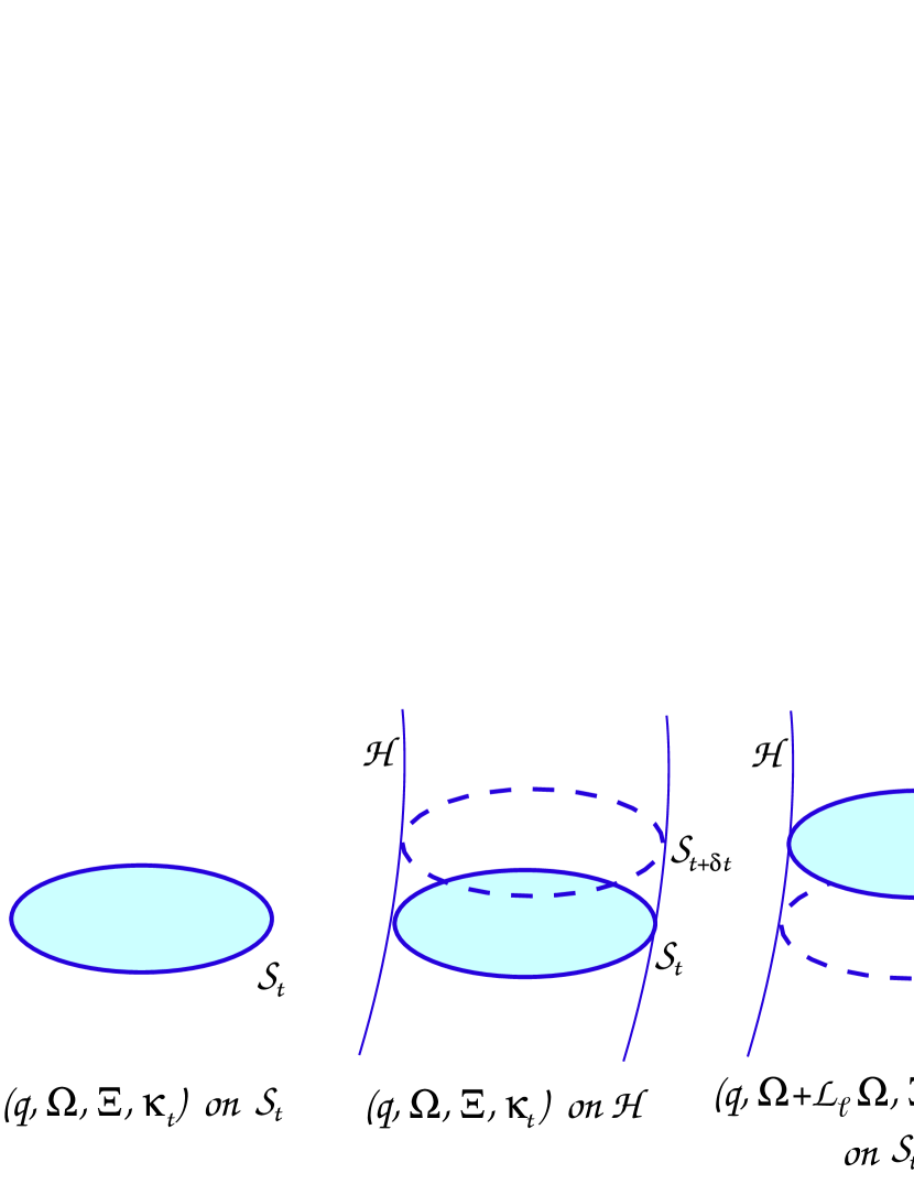
Figure 7.1: Reconstruction of the NEH from the free data. Left: choice of free data on ${\mathcal{S}}_{t}$. Center: Free data as fields on ${\mathcal{H}}$. Right: Evolution of the free data to a infinitesimally close surface ${\mathcal{S}}_{t+\delta t}$.

7.7.2 Reconstruction of ${\mathcal{H}}$ from data on ${\mathcal{S}}_{t}$. Free data

Let us describe how a NEH may be reconstructed from data on an initial spatial slice ${\mathcal{S}}_{t}$. We proceed in three steps (see Fig. 7.1). Firstly, a free choice for the values of $(\bm{q},\bm{\Omega},\kappa$, $\bm{\Xi})$ on ${\mathcal{S}}_{t}$ is made, considering them as objects intrinsic to ${\mathcal{S}}_{t}$. Secondly, these objects are regarded as fields living in ${\mathcal{H}}$ by imposing, on the slice ${\mathcal{S}}_{t}$, the vanishing of their corresponding null components:

$$\bm{\ell}\cdot\bm{q}=0\ \ \ \ \bm{\ell}\cdot\bm{\Omega}=0\ \ \ \ \bm{\ell}\cdot\bm{\Xi}=0\ .$$ (7.74)

Finally, the value of these fields is calculated in an infinitesimally close slice ${\mathcal{S}}_{t+\delta t}$ by employing Eqs. (7.7.1). The value of $\kappa$ on ${\mathcal{S}}_{t+\delta t}$ can be chosen freely again. We note by passing that the expression $\bm{\hat{\nabla}}\bm{\ell}=\bm{\ell}\otimes\bm{\omega}$ [Eq. (7.25)], which can be seen as a constraint on the NEH geometry, is automatically satisfied by following the above procedure, since ${\bm{\ell}}$ is torsion free (being normal to ${\mathcal{H}}$) and we construct a vanishing $\bm{\Theta}$. It is not an independent constraint.

We conclude that the free data for the null NEH geometry are given by

$$\framebox{$\displaystyle\hbox{NEH-free data:}\ \ \ (\bm{q}|_{{\mathcal{S}}_{t}},\bm{\Omega}|_{{\mathcal{S}}_{t}},\bm{\Xi}|_{{\mathcal{S}}_{t}},\kappa|_{{\mathcal{H}}})$}\ .$$ (7.75)

That is, the initial data $\bm{q}$, $\bm{\Omega}$ and $\bm{\Xi}$ on ${\mathcal{S}}_{t}$, together with the function $\kappa$ on ${\mathcal{H}}$, can be freely specified. This is in contrast with the $3+1$ Cauchy problem, where the initial data on the spatial slice $\Sigma_{t}$ are in fact constrained (cf. Sec. 3.6). Once the free data are given, the full geometry in ${\mathcal{H}}$ can be reconstructed by evolving these quantities along $\bm{\ell}$, this null normal being determined through Eq. (4.13) by the additional structure provided by the slicing $(\Sigma_{t})$. Therefore, for a given null geometry $(\bm{q},\bm{\hat{\nabla}})$, their initial data $(\bm{q}|_{{\mathcal{S}}_{t}},\bm{\Omega}|_{{\mathcal{S}}_{t}},\bm{\Xi}|_{{\mathcal{S}}_{t}},\kappa|_{{\mathcal{H}}})$ are associated with a particular $\bm{\ell}=N(\bm{n}+\bm{s})$ (see below).

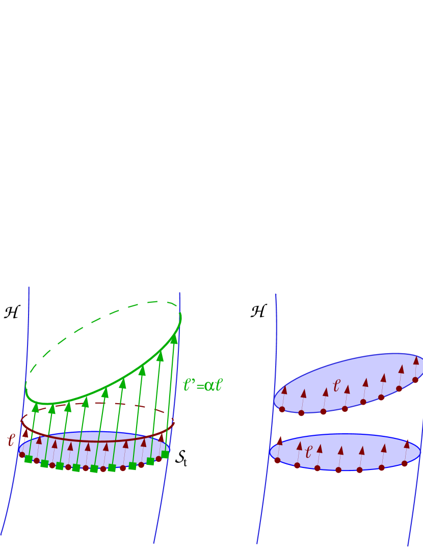
Figure 7.2: On the left the active aspect of the gauge freedom, linked to the choice of the null normal, and on the right the passive aspect, associated with the choice of a initial slice.

Gauge freedom in the choice of the free data

Even though each specific choice of data in (7.75), together with a slicing $(\Sigma_{t})$, fixes the NEH geometry, there are different choices that actually define the same NEH structure: there exists a degeneracy in the free data that can be referred to as a gauge freedom. This degeneration presents two aspects, the first one linked to the choice of the null normal, and the second one to the slicing of ${\mathcal{H}}$ once $\bm{\ell}$ is fixed (see Fig. 7.2):

• If we start from a fixed slice ${\mathcal{S}}_{0}$, our choice of $(\bm{q},\bm{\Omega},\kappa$, $\bm{\Xi})$ is, as mentioned above, associated with a particular null vector $\bm{\ell}$. However, the NEH geometry is not changed under a rescaling $\alpha$ of the null normal, $\bm{\ell}^{\prime}=\alpha\bm{\ell}$. Under this rescaling, the fields $(\bm{q},\bm{\Omega},\bm{\Xi},\kappa)$ change according to the transformations given in Table 5.1. The resulting intrinsic null geometry $(\bm{q},\bm{\hat{\nabla}})$ is the same, even though the slicings $({\mathcal{S}}_{t})$ and $({\mathcal{S}}_{t^{\prime}})$ of ${\mathcal{H}}$ induced by the transport of ${\mathcal{S}}_{0}$ along $\bm{\ell}$ and $\bm{\ell}^{\prime}$ will in general differ. We will call this ambiguity the active aspect of the gauge freedom. It is associated with the fact that different slicings $(\Sigma_{t})$ fix (in general) different null normals $\bm{\ell}$ via Eq. (4.13), and it is a natural gauge freedom when one actually constructs ${\mathcal{H}}$ starting from a slice ${\mathcal{S}}_{0}$ as in a Cauchy problem.

• Even though a slicing $(\Sigma_{t})$ fixes $\bm{\ell}$ the reverse is not true, since this null normal is compatible with different spatial slicings. Keeping $\bm{\ell}$ fixed, we can consider initial slices ${\mathcal{S}}_{0}$ and ${\mathcal{S}}^{\prime}_{0}$ in ${\mathcal{H}}$ belonging to different slicings $({\mathcal{S}}_{t})$ and $({\mathcal{S}}_{t^{\prime}})$ of ${\mathcal{H}}$ compatible with $\bm{\ell}$ via (4.6). The corresponding level functions $t$ and $t^{\prime}$ are related by $\bm{\hat{\nabla}}t=\bm{\hat{\nabla}}t^{\prime}-\bm{\hat{\nabla}}g$, where ${}^{{\mathcal{H}}}\!\bm{\mathcal{L}}_{\bm{\bm{\ell}}}\,g=0$. This change in the slicing does not affect $\bm{q}$, $\bm{\ell}$, $\bm{\omega}$ and consequently $\kappa$, but induces via Eq. (4.34) the transformations (cf. Eq. (3.10) in [13])

  $$\underline{\bm{k}}\rightarrow\underline{\bm{k}}+\bm{\hat{\nabla}}g\ \ ,\ \ \bm{\Omega}\rightarrow\bm{\Omega}-\kappa\bm{\hat{\nabla}}g\ \ ,\ \ \bm{\Xi}\rightarrow\bm{\Xi}+\bm{\hat{\nabla}}\bm{\hat{\nabla}}g\ .$$ (7.76)

  This aspect of the gauge freedom, that we can refer to as passive and which corresponds to a coordinate choice in ${\mathcal{H}}$, is natural when ${\mathcal{H}}$ is a hypersurface existing a priori, its slicings only entering in a second step once $\bm{\ell}$ is fixed. It is the aspect discussed in Refs. [13, 108].

In brief, from a 3+1 perspective, in both cases the underlying source of degeneracy in the free data is related to the choice of a specific slicing of ${\mathcal{H}}$. When there is no canonical manner of fixing neither the initial slice nor the null vector $\bm{\ell}$, as it is the case in a purely intrinsic formulation of the geometry of ${\mathcal{H}}$, both sources of gauge freedom are simultaneously present (see discussion in Section VI.A.2 of Ref. [111]).

7.7.3 Evolution of $\hat{\nabla}$ from an intrinsic null perspective

Following the 3+1 approach adopted in this article, the previous discussion on the NEH-constraints has made explicit use of a spatial slicing of ${\mathcal{H}}$. However, the time evolution of the connection $\bm{\hat{\nabla}}$ can be described in a more intrinsic manner. In order to prepare the notion of (strongly) isolated horizon in Section 9.1, we briefly comment on it.

The evolution of the connection $\bm{\hat{\nabla}}$ along $\bm{\ell}$ can be written (in components) as follows (see Refs. [13, 111])

$$[{}^{{\mathcal{H}}}\!\bm{\mathcal{L}}_{\bm{l}}\,,\hat{\nabla}_{\alpha}]\varpi_{\beta}=-N_{\alpha\beta}\ell^{\mu}\varpi_{\mu}$$ (7.77)

for any 1-form $\bm{\varpi}\in{\mathcal{T}}^{*}({\mathcal{H}})$, where

$$N_{\alpha\beta}=\hat{\nabla}_{(\alpha}\omega_{\beta)}+\omega_{\alpha}\omega_{\beta}+\frac{1}{2}\left(R_{\alpha\beta}-{}^{2}\!R_{\alpha\beta}\right)\ .$$ (7.78)

Together with the evolution for $\bm{q}$ in Eq. (7.12), these evolution equations constitute the geometrical identities involving only $\bm{q},\bm{\hat{\nabla}}$ and $\bm{R}$, i.e. they provide the NEH constraints.

Following the procedure in the isolated horizon literature [13, 111], we introduce the following tensor on ${\mathcal{H}}$

$$\bm{S}:=\Phi^{*}\bm{\nabla}\underline{\bm{k}}\ ,$$ (7.79)

where $\underline{\bm{k}}$ is associated with a foliation compatible with $\bm{\ell}$. According to Eq. (4.34), $\Phi^{*}\underline{\bm{k}}$ is exact on ${\mathcal{H}}$ implying that $\bm{S}$ is symmetric. In addition, $\vec{\bm{q}}^{*}\bm{S}=\bm{\Xi}$ and $\bm{\ell}\bm{\cdot S}=\bm{\omega}$ (see Eqs. (5.80) and (5.86), respectively). From the discussion in Secs. 7.7.1 and 7.7.2, it follows that the evolution of $\bm{\hat{\nabla}}$ is given by that of the pair $(\bm{q},\bm{S})$. Making $\bm{\varpi}$ equal to $\underline{\bm{k}}$ in Eq. (7.77), one obtains

$${}^{{\mathcal{H}}}\!{\mathcal{L}}_{\bm{\bm{\ell}}}\,S_{\alpha\beta}=N_{\alpha\beta}\ ,$$ (7.80)

thus providing the evolution equation for $\bm{S}$. The NEH-constraints are now

$${}^{{\mathcal{S}}}\!\bm{\mathcal{L}}_{\bm{\bm{\ell}}}\,\bm{q} = 0$$ (7.81)

$${}^{{\mathcal{H}}}\!{\mathcal{L}}_{\bm{\bm{\ell}}}\,S_{\alpha\beta} = \hat{\nabla}_{(\alpha}\omega_{\beta)}+\omega_{\alpha}\omega_{\beta}+\frac{1}{2}\left(R_{\alpha\beta}-{}^{2}\!R_{\alpha\beta}\right)$$ (7.82)

Contracting the second one with $\bm{\ell}$, Eq. (7.44) for the evolution of $\bm{\omega}$ is recovered, whereas the projection onto a slice ${\mathcal{S}}_{t}$ leads to the evolution equation (7.33) for $\bm{\Xi}$.

8 Isolated horizons I: weakly isolated horizons

8.1 Introduction

The NEH notion introduced in the previous section, represents a first step toward the quasi-local characterization of a black hole horizon in equilibrium. As we have seen, this is achieved essentially by imposing a condition on the degenerate metric $\bm{q}$, namely to be time-independent [Eq. (7.12)].

This minimal geometrical condition captures some fundamental features of a black hole in quasi-equilibrium. On the one hand, it is sufficiently flexible so as to accommodate a variety of interesting physical scenarios. But on the other hand, such a structure is not tight enough to determine some geometrical and physical properties of a black hole horizon. From the point of view of the geometry of ${\mathcal{H}}$ as a hypersurface in ${\mathcal{M}}$, the NEH notion by itself provides a limited set of tools to extract information about the spacetime containing the black hole. For instance, it does not pick up any particular normalization of the null normal nor suggest any concrete foliation of ${\mathcal{H}}$, something that was accomplished in the previous sections by using the additional structure $(\Sigma_{t})$. Since in the spacetime construction as a Cauchy problem, the 3+1 foliation is actually dynamically determined, it would be very useful to dispose of a slicing $({\mathcal{S}}_{t})$ motivated from an intrinsic analysis of ${\mathcal{H}}$ and that one can employ as an inner boundary condition for $(\Sigma_{t})$. Regarding the determination of physical black hole parameters, a point of evident astrophysical interest, a NEH does not determine any prescription for the mass, the angular momentum or, more generally, for the black hole multipole moments.

In order to address these issues, i.e. the discussion of the horizon properties from a point of view intrinsic to ${\mathcal{H}}$, we need a finer characterization of the notion of quasi-equilibrium. Following Ashtekar et al. [13], this demands the introduction of additional structures on ${\mathcal{H}}$. After imposing the degenerate metric $\bm{q}$ to be time-independent, a natural way to proceed in order to further constrain the horizon geometry consists in extending this condition to the rest of the geometrical objects on ${\mathcal{H}}$, in particular to the induced connection $\bm{\hat{\nabla}}$. This strategy directly leads to the introduction of a hierarchy of quasi-equilibrium structures on the horizon, which turns out to be very useful for keeping control of the physical and geometrical hypotheses actually assumed. A particularly clear synthesis of the resulting formalism can be found in Refs. [111, 107].

The pair of fields $(\bm{q},\bm{\hat{\nabla}})$, or equivalently $(\bm{q},\bm{\Omega},\kappa$, $\bm{\Xi})$ (see Sec. 7.7), characterizes the geometry of a NEH (cf. Remark 7.5). From a 3+1 perspective, and following the strategy previously outlined, a natural manner of obtaining different degrees of quasi-equilibrium for the horizon would consist in imposing the time independence of different combinations of the fields $(\bm{q},\bm{\Omega},\kappa$, $\bm{\Xi})$. However, the resulting notions of horizon quasi-equilibrium would be slicing-dependent. Even though in Sec. 9.2 we will revisit this idea, we rather proceed here by constructing the new structures on ${\mathcal{H}}$ on the grounds of fields intrinsic to ${\mathcal{H}}$. Once the time independence of $\bm{q}$ has been used to define a NEH, this means imposing time independence on the full connection $\bm{\hat{\nabla}}$ or, in a intermediate step, on its component $\bm{\omega}$. This defines the three levels in the (intrinsic) isolated horizon hierarchy.

We separate the study of the isolated horizons in two sections. In the present one, we focus on the intermediate level resulting from the introduction, in a consistent way, of a time-independent rotation 1-form $\bm{\omega}$. This second level in the isolated horizon hierarchy leads to the notion of weakly isolated horizon (WIH). After introducing in Sec. 8.2 its definition and straightforward consequences, Secs. 8.3, 8.4 and 8.5 are devoted to different implications on the null geometry of ${\mathcal{H}}$. Finally Sec. 8.6 briefly presents how a WIH structure permits to determine the physical parameters associated with the black hole horizon. The stronger level in the isolated horizon hierarchy, which results from a full time-independent $\bm{\hat{\nabla}}$ , will be discussed in Sec. 9, where we will also comment on other developments naturally related to the isolated horizon structures.

8.2 Basic properties of weakly isolated horizons

8.2.1 Definition

As already noticed, the NEH notion is independent of the rescaling of the null normal $\bm{\ell}$. On the contrary, imposing the constancy of the rotation 1-form $\bm{\omega}$ [the part of $\bm{\hat{\nabla}}$ along $\bm{\ell}$, cf. Eq. (7.7.1)] under the flow of the null normal, does depend on the actual choice for $\bm{\ell}$. This is a consequence of the transformation of $\bm{\omega}$ under a rescaling of $\bm{\ell}$ (cf. Table 5.1):

$$\bm{\omega}\stackrel{{\scriptstyle\bm{\ell}\to\alpha\bm{\ell}}}{{\longrightarrow}}\bm{\omega}+\bm{\Pi}^{*}\bm{\mathrm{d}}\ln\alpha\ .$$ (8.1)

If we consider a null normal $\bm{\ell}$ such that ${}^{{\mathcal{H}}}\!\bm{\mathcal{L}}_{\bm{\bm{\ell}}}\,\bm{\omega}=0$ then, after a rescaling of $\bm{\ell}$ by some non-constant $\alpha$, the new rotation 1-form will not be time-independent in general. In order to make sense of condition ${}^{{\mathcal{H}}}\!\bm{\mathcal{L}}_{\bm{\bm{\ell}}}\,\bm{\omega}=0$, we must restrict the set of the null normals for which it actually applies. From Eq. (8.1) we conclude that if $\bm{\omega}$ is invariant under a given null normal $\bm{\ell}$, then it is also invariant under any constant rescaling of it (this could be relaxed to time-independent functions). This is formalized by the following definitions [15, 13]:

• Two null normals $\bm{\ell}$ and $\bm{\ell}^{\prime}$ are said to be related to each other if and only if $\bm{\ell}^{\prime}=c\,\bm{\ell}$ with $c$ a positive constant. This defines an equivalence relation whose equivalence classes are denoted by $[\bm{\ell}]$.

• A weakly isolated horizon (WIH) $({\mathcal{H}},[\bm{\ell}])$ is a NEH ${\mathcal{H}}$ endowed with an equivalence class $[\bm{\ell}]$ of null normals such that

  $$\framebox{$\displaystyle{}^{{\mathcal{H}}}\!\bm{\mathcal{L}}_{\bm{\bm{\ell}}}\,\bm{\omega}=0$}.$$ (8.2)

We comment on some consequences of this definition.

1. Extremal and non-extremal WIH. As a consequence of the transformation rule for $\kappa$ under a rescaling of $\bm{\ell}$ (cf. Table 5.1), two null normals $\bm{\ell}$ and $\bm{\ell}^{\prime}$ belonging to the same WIH class have non-affinity coefficients $\kappa_{(\bm{\ell})}$ and $\kappa_{(\bm{\ell}^{\prime})}$ related by

$$\kappa_{(\bm{\ell}^{\prime})}=c\,\kappa_{(\bm{\ell})},$$ (8.3)

where $c$ is the constant linking the two null vectors: $\bm{\ell}^{\prime}=c\,\bm{\ell}$. This implies that there is no canonical value of the non-affinity coefficient $\kappa$ on a given WIH. This reflects the absence of canonical representative in the class $[\bm{\ell}]$. We have already presented a solution to this point, relying on the 3+1 spacelike slicing in Sec. 4.2. We will present another solution, intrinsic to ${\mathcal{H}}$, in Sec. 8.6. The transformation law (8.3) means that, on a given NEH, the WIH structures are naturally divided in two types: those with vanishing $\kappa_{(\bm{\ell})}$, that will be referred as extremal WIHs, and those with $\kappa_{(\bm{\ell})}\neq 0$, non-extremal WIHs. This terminology arises from the Kerr spacetime, where one can always choose the null normal $\bm{\ell}$ to let it coincide with a Killing vector field. Then $\kappa_{(\bm{\ell})}$ is nothing but the surface gravity of the black hole [cf. Eq. (2.48) in Example 2.5 for the non-rotating case and Eq. (D.34) in Appendix D for the general case]. Extreme Kerr black holes are those for which the surface gravity vanishes. As shown by Eq. (D.34), this corresponds to the angular momentum parameter $a/m=1$. They are not expected to exist in the Universe, because it is not possible to make a black hole rotate faster than $a/m=0.998$ by standard astrophysical processes (i.e. infall of matter from an accretion disk [164]). In this article, we will focus on the non-extremal case, and refer the reader to [13, 111] for the general case.

2. Constancy of the surface gravity on $\mathcal{H}$. From the NEH Eq. (7.67)

$$\bm{\ell}\cdot{}^{\mathcal{H}}\bm{\mathrm{d}}\bm{\omega}=0,$$ (8.4)

and using the Cartan identity (1.26) on ${\mathcal{H}}$:

$$0={}^{{\mathcal{H}}}\!\bm{\mathcal{L}}_{\bm{\bm{\ell}}}\,\bm{\omega}=\bm{\ell}\cdot{}^{\mathcal{H}}\bm{\mathrm{d}}\bm{\omega}+{}^{\mathcal{H}}\bm{\mathrm{d}}\langle\bm{\ell},\bm{\omega}\rangle={}^{\mathcal{H}}\bm{\mathrm{d}}\kappa_{(\bm{\ell})}\ \Leftrightarrow\framebox{$\displaystyle\bm{\hat{\nabla}}\kappa_{(\bm{\ell})}=0$}.$$ (8.5)

Therefore, the non-affinity coefficient of a given $\bm{\ell}$ is a constant on ${\mathcal{H}}$. This property, that is referred to as the zeroth law of black hole mechanics, characterizes $[\bm{\ell}]$ as associated with a WIH structure. It will be discussed further in Remark 8.3 below.

3. Any NEH admits a WIH structure. We have just seen that the class $[\bm{\ell}]$ associated with $\bm{\ell}$ is a WIH structure if and only if $\kappa_{(\bm{\ell})}$ is a constant on ${\mathcal{H}}$. In Secs. 7.7 and 7.7.2 we established that a given NEH geometry is determined by the set of fields $(\bm{q},\bm{\Omega},\kappa_{(\bm{\ell})}$, $\bm{\Xi})$, where $\kappa_{(\bm{\ell})}$ is an arbitrary function, and also by any other set obtained from this one by applying the transformations in Table 5.1. This was called the active aspect of the gauge freedom in the NEH-free data, and it simply corresponds to a rescaling by $\alpha$ of the null normal $\bm{\ell}$. Therefore if, according to Eq. (2.26), we choose $\alpha$ satisfying

$$\kappa^{\prime}=\bm{\nabla}_{\bm{\ell}}\alpha+\alpha\kappa_{(\bm{\ell})}$$ (8.6)

with $\kappa^{\prime}$ constant on ${\mathcal{H}}$, then $[\bm{\ell}^{\prime}]$ given by $\bm{\ell}^{\prime}=\alpha\bm{\ell}$ constitutes a WIH class (in particular, making $\kappa^{\prime}=0$ shows that any NEH admits an extremal horizon; Sec. III.A of Ref. [13] firstly shows the existence of an extremal WIH for any NEH, and then constructs from it a family of non-extremal ones). As a consequence, the addition of a WIH does not represent an actual constraint on the null geometry of ${\mathcal{H}}$. It rather distinguishes certain classes of null normals.

4. Infinite freedom of the WIH structure. Not only it is always possible to choose a WIH structure on a NEH, but there exists actually an infinite number of non-equivalent WIHs. Reasoning for the non-extremal case, if $\bm{\ell}$ is such that $\kappa_{(\bm{\ell})}$ is a non-vanishing constant on ${\mathcal{H}}$ and $t$ is a coordinate on ${\mathcal{H}}$ compatible with $\bm{\ell}$, i.e. ${}^{{\mathcal{H}}}\!\bm{\mathcal{L}}_{\bm{\bm{\ell}}}\,t=1$, then the class $[\bm{\ell}^{\prime}]$ associated with the vector $\bm{\ell}^{\prime}$ defined by

$$\bm{\ell}^{\prime} = \left(1+Be^{-\kappa_{(\bm{\ell})}t}\right)\bm{\ell}$$ (8.8)

$${}^{{\mathcal{H}}}\!\bm{\mathcal{L}}_{\bm{\bm{\ell}}}\,B=0\ ,$$

is distinct from the class $[\bm{\ell}]$ (for $\alpha:=1+B\e^{-\kappa_{(\bm{\ell})}t}$ is not constant) and also defines a WIH. This follows from $\kappa_{(\bm{\ell}^{\prime})}=\kappa_{(\bm{\ell})}=\mathrm{const}$. Using the slicing $({\mathcal{S}}_{t})$ induced on ${\mathcal{H}}$ from the $3+1$ decomposition, the functions $B$ in Eq. (8.8) have actually support on the sections ${\mathcal{S}}_{t}$ and parametrize the different WIH structures. In an analogous manner for the extremal case, $\kappa_{(\bm{\ell})}=0$, the non-equivalent rescaled null normal $\bm{\ell}^{\prime}=A\bm{\ell}$ with $A$ a non-constant function on $\mathcal{S}_{t}$, is also associated with a non-equivalent extremal WIH.

8.2.2 Link with the 3+1 slicing

Since a WIH structure does not further constrain the geometry of ${\mathcal{H}}$, from a quasi-equilibrium point of view a WIH is not more isolated than a NEH. However, this notion presents a remarkable richness as a structural tool. In this sense its interest is two-fold, both from a geometrical and physical point of view. In addition, this concept provides a natural framework to discuss the interplay between the horizon ${\mathcal{H}}$ and the spatial 3+1 foliation $(\Sigma_{t})$, something specially relevant in our approach. In this last sense, the issue of the compatibility between the structures intrinsically defined on ${\mathcal{H}}$ and the additional one provided by the 3+1 slicing of the spacetime, is naturally posed.

Given a WIH $({\mathcal{H}},[\bm{\ell}])$, a 3+1 slicing $(\Sigma_{t})$ is called WIH-compatible if there exists a representative $\bm{\ell}$ in $[\bm{\ell}]$ such that the associated level function $t$ evaluated on the horizon ${\mathcal{H}}$ constitutes a natural coordinate for $\bm{\ell}$, i.e. ${\mathcal{L}}_{\bm{\ell}}t=1$ [99]. Note that the representative $\bm{\ell}$ is then nothing but the null normal associated with the slicing $({\mathcal{S}}_{t})$ of ${\mathcal{H}}$ by the normalization (4.6).

Given independently a NEH ${\mathcal{H}}$ and a 3+1 slicing of ${\mathcal{M}}$, there is no guarantee that there exists a WIH structure on the NEH such that $(\Sigma_{t})$ is WIH-compatible. If such a WIH exists, $\bm{\ell}$ is tied to the $t$ function and therefore to the slicing. If not, no relation exists between that WIH and $(\Sigma_{t})$. Therefore, even though the choice of a specific WIH structure on our NEH does not affect the intrinsic geometry of the horizon, demanding the 3+1-slicing to be WIH-compatible represents an actual restriction on the 3+1 description of spacetime (see Sec. 11.3.1). And this fact is crucial in our approach: some of the possible spacetimes slicings are directly ruled out.

We have noticed in Remark 7.6 that, on a NEH, the Háj́iček 1-form $\bm{\Omega}$ (more concretely its divergence) is an object directly depending upon the 3+1 slicing, whereas the rotation 1-form $\bm{\omega}$ depends only upon the normalization of $\bm{\ell}$. Let us then investigate the consequences of the WIH condition on $\bm{\Omega}$. From Eq. (7.40), we have

$${}^{{\mathcal{H}}}\!\bm{\mathcal{L}}_{\bm{\bm{\ell}}}\,\bm{\omega}={}^{{\mathcal{H}}}\!\bm{\mathcal{L}}_{\bm{\bm{\ell}}}\,\bm{\Omega}-\left({}^{{\mathcal{H}}}\!\bm{\mathcal{L}}_{\bm{\bm{\ell}}}\,\kappa_{(\bm{\ell})}\right)\,\Phi^{*}\underline{\bm{k}},$$ (8.9)

where we have considered both $\bm{\omega}$ and $\bm{\Omega}$ as a 1-forms in ${\mathcal{T}}^{*}({\mathcal{H}})$ (identifying them with their pull-back $\Phi^{*}\bm{\omega}$ and $\Phi^{*}\bm{\Omega}$). In view of the above relation, we deduce from Eqs. (8.2) and (8.5) that

$$\framebox{$\displaystyle(\mbox{$({\mathcal{H}},[\bm{\ell}])$ is a WIH})\iff\left\{\begin{array}[]{l}{}^{{\mathcal{H}}}\!\bm{\mathcal{L}}_{\bm{\bm{\ell}}}\,\bm{\Omega}=0\\ {}^{{\mathcal{H}}}\!\bm{\mathcal{L}}_{\bm{\bm{\ell}}}\,\kappa_{(\bm{\ell})}=0\end{array}\right.$}.$$ (8.10)

Note that ${}^{{\mathcal{H}}}\!\bm{\mathcal{L}}_{\bm{\bm{\ell}}}\,\kappa_{(\bm{\ell})}=0$ is listed here, along with ${}^{{\mathcal{H}}}\!\bm{\mathcal{L}}_{\bm{\bm{\ell}}}\,\bm{\Omega}=0$, as a sufficient condition to have a WIH, but once the WIH structure holds, one has actually the much stronger property of constancy of $\kappa_{(\bm{\ell})}$ on all ${\mathcal{H}}$ [zeroth law, Eq. (8.5)].

8.2.3 WIH-symmetries

The discussion of the physical parameters of the black hole horizon in Sec. 8.6 demands the introduction of the notion of a symmetry related to a WIH horizon. We present a brief account of it, with emphasis in the non-extremal case and refer the reader to Refs. [12, 107] for details and extensions.

A symmetry of a WIH is a diffeomorphism of ${\mathcal{H}}$ preserving the relevant structures of the WIH. Infinitesimally this is captured as follows: a vector field $\bm{W}$ tangent to ${\mathcal{H}}$ is said to be an infinitesimal WIH-symmetry of $({\mathcal{H}},[\bm{\ell}])$, if it preserves the equivalence class of null normals, the metric $\bm{q}$ and the 1-form $\bm{\omega}$, namely

$${}^{{\mathcal{H}}}\!\bm{\mathcal{L}}_{\bm{W}}\,\bm{\ell}=\mathrm{const}\cdot\bm{\ell},\ \ \ {}^{{\mathcal{H}}}\!\bm{\mathcal{L}}_{\bm{W}}\,\bm{q}=0\ \ \ \mbox{and}\ \ \ {}^{{\mathcal{H}}}\!\bm{\mathcal{L}}_{\bm{W}}\,\bm{\omega}=0\,.$$ (8.11)

In the considered non-extremal case, the general form of such a WIH symmetry is given by (see Sec. III in [12])

$$\bm{W}=c_{\bm{W}}\bm{\ell}+b_{\bm{W}}\bm{S}\,,$$ (8.12)

where $c_{\bm{W}}$ and $b_{\bm{W}}$ are constant on ${\mathcal{H}}$ and the vector field $\bm{S}$, satisfying $\bm{\ell}\cdot\bm{S}=0$, is an isometry on each section $({\mathcal{S}}_{t},\bm{q})$. From this general form of an infinitesimal symmetry, and according to the number of independent generators in the associated Lie algebra of symmetries, one can distinguish different universality classes of WIH-symmetries. Since $\bm{\ell}\in[\bm{\ell}]$ is an infinitesimal symmetry by construction, the Lie algebra (and therefore the Lie group) of WIH-symmetries is always at least one-dimensional:

• Class I. The symmetry Lie algebra is generated by $\bm{\ell}$ together with the infinitesimal rotations acting on the 2-sphere ${\mathcal{S}}_{t}$. The resulting group is the direct product of $SO(3)$ and the translations in the $\bm{\ell}$ direction. This case corresponds to the horizon of a non-rotating black hole.

• Class II. The symmetry group is now the direct product of the translations along $\bm{\ell}$ and an axial $SO(2)$ symmetry on ${\mathcal{S}}_{t}$. It corresponds to an axisymmetric horizon and represents the most interesting physical case, since it corresponds to a black hole with well-defined non-vanishing angular momentum (see Sec. 8.6).

• Class III. The symmetry group is one-dimensional (translations along $\bm{\ell}$). It corresponds to the general distorted case.

Note that I is a special case of II, and the latter is a special case of III.

8.3 Initial (free) data of a WIH

As commented in the point 3. after the WIH definition, the geometry of a WIH as a null hypersurface is that of a NEH. In particular, the free data of a WIH are essentially those presented in Sec. 7.7 for a NEH. The only difference is the choice of a null normal $\bm{\ell}$ such that the zeroth law (8.5) is satisfied and, consequently, $\kappa_{(\bm{\ell})}$ is constant on ${\mathcal{H}}$, $\kappa_{o}$:

$$\framebox{$\displaystyle\hbox{WIH-free initial data:}\ \ \ (\bm{q}|_{{\mathcal{S}}_{t}},\bm{\Omega}|_{{\mathcal{S}}_{t}},\bm{\Xi}|_{{\mathcal{S}}_{t}},\kappa_{o})$}\ .$$ (8.13)

We note that, since in a WIH the null normal $[\bm{\ell}]$ is fixed up to a constant, the gauge freedom in the WIH-free data concerns mainly what we called the passive aspect in Sec. 7.7.2 . The active one reduces to constant rescalings of $\kappa_{(\bm{\ell})}$ and $\bm{\Xi}$. Once these free data are fixed on ${\mathcal{S}}_{t}$, the reconstruction of the WIH on ${\mathcal{H}}$ proceeds as in Sec. 7.7.2. The only subtlety now enters in the third step represented in Fig. 7.1, when the fields on the slice ${\mathcal{S}}_{t}$ are transported to the next slice. In the construction of the WIH not only the metric $\bm{q}$ is Lie dragged by $\bm{\ell}$, but also the Háj́iček form $\bm{\Omega}$ and the non-affinity coefficient $\kappa_{o}$, as shown by Eq. (8.10). Now, the only field evolving in time is $\bm{\Xi}$.

In view of Eq. (7.33) and the time-independence of $\bm{q}$ (hence of $\bm{{}^{2}\!D}$ and ${}^{2}\!\bm{R}$), $\bm{\Omega}$ and $\kappa$, the time dependence of $\bm{\Xi}$ can be explicitly integrated if we assume that the projection of the 4-dimensional Ricci tensor (or the matter stress-energy tensor via the Einstein equation) is time-independent, i.e.

$$\bm{\Pi}^{*}\bm{\mathcal{L}}_{\bm{\bm{\ell}}}\,\bm{R}=0\ .$$ (8.14)

In fact, this condition is actually well-defined on a NEH, i.e. it does not depend on the choice of the null normal $\bm{\ell}$. This follows from property (7.32). Condition (8.14) is rather mild and is obviously satisfied in a vacuum spacetime. If we deal with a WIH built on a NEH that fulfills (8.14), then in the evolution of $\bm{\Xi}$ dictated by Eq. (7.33) the only terms which depend on time are $\bm{\Xi}$ and ${}^{{\mathcal{H}}}\!\bm{\mathcal{L}}_{\bm{\bm{\ell}}}\,\bm{\Xi}$. In this situation, and assuming a non-extremal WIH ($\kappa_{(\bm{\ell})}\not=0$), this equation can be straightforwardly integrated [13], resulting in

$$\bm{\Xi} = e^{-\kappa_{(\bm{\ell})}t}\,\bm{\Xi}^{0}+\frac{1}{\kappa_{(\bm{\ell})}}\left[\frac{1}{2}\,{\rm Kil}(\bm{{}^{2}\!D},\bm{\Omega})+\bm{\Omega}\otimes\bm{\Omega}-\frac{1}{2}{}^{2}\!\bm{R}+4\pi\left(\vec{\bm{q}}^{*}\bm{T}-\frac{T}{2}\bm{q}\right)\right],$$

where $\bm{\Xi}^{0}$ is the integration constant, a time-independent symmetric tensor, and $t$ is a coordinate on ${\mathcal{H}}$ compatible with $\bm{\ell}$ via Eq. (4.6), i.e. $\bm{\mathcal{L}}_{\bm{\bm{\ell}}}\,t=1$.

8.4 Preferred WIH class $[\bm{\ell}]$

We have seen that a NEH admits an infinite number of WIH structures which, in the non-extremal case and according to (8.8), are parametrized by functions $B$ defined on ${\mathcal{S}}_{t}$. The question about the existence of a natural choice among them is naturally posed.

In case we dispose of an a priori slicing $(\Sigma_{t})$ of ${\mathcal{M}}$, a slicing $({\mathcal{S}}_{t})$ of the horizon is determined independently of the geometrical structures defined on ${\mathcal{H}}$, as discussed in Sec. 4. Such a slicing fixes the null normal $\bm{\ell}$ via the normalization (4.6) [or, equivalently, the slicing fixes the lapse $N$ and $N$ determines $\bm{\ell}$ by Eq. (4.13)]. If the slicing is a WIH-compatible one, a particular class $[\bm{\ell}]$ is chosen. If not, such a slicing does not help in making such a choice.

More interesting is, however, the opposite situation, which occurs whenever the 3+1 slicing $(\Sigma_{t})$ is determined in a dynamical way. In such a context, an intrinsic determination of a preferred WIH class helps in the very construction of the 3+1 slicing. In fact, if such a WIH class is provided together with a definite initial cross section ${\mathcal{S}}_{0}$, then the slicing $({\mathcal{S}}_{t})$ of ${\mathcal{H}}$ is completely determined, and can be used as a boundary condition to fix $(\Sigma_{t})$.

From an intrinsic point of view, fixing the class $[\bm{\ell}]$ reduces to choosing the function $B$ in Eq. (8.8). Such a choice can be made by imposing a condition on a scalar definable in terms of the fields defining the WIH geometry. Following [13], an appropriate scalar in this sense is provided by the trace of ${}^{{\mathcal{H}}}\!\bm{\mathcal{L}}_{\bm{\bm{\ell}}}\,\bm{\Xi}$ which, on a NEH, corresponds to the Lie derivative in the $\bm{\ell}$ direction of the expansion $\theta_{(\bm{k})}$ associated with the ingoing null normal $\bm{k}$ [cf. Eq. (5.87)]. Contracting equation (7.33) with $\bm{q}$ yields

$$\bm{\mathcal{L}}_{\bm{\bm{\ell}}}\,\theta_{(\bm{k})}={}^{2}\!D^{\mu}\Omega_{\mu}+\Omega_{\mu}\Omega^{\mu}-\frac{1}{2}{}^{2}\!R+\frac{1}{2}q^{\mu\nu}R_{\mu\nu}-\kappa\theta_{(\bm{k})}.$$ (8.16)

We start with a WIH with null normal $\bm{\ell}$ and free data $(\bm{q},\bm{\Omega},\bm{\Xi},\kappa_{(\bm{\ell})})$. Firstly we notice that, if condition (8.14) holds, the value of $\bm{\mathcal{L}}_{\bm{\bm{\ell}}}\,\theta_{(\bm{k})}$ at $t=0$ resulting from Eq. (8.3) satisfies (where $\Xi^{0}_{\mu\nu}$ are constant)

$$\left.\bm{\mathcal{L}}_{\bm{\bm{\ell}}}\,\theta_{(\bm{k})}\right|_{t=0}=-\kappa_{(\bm{\ell})}\left(q^{\mu\nu}\,\Xi^{0}_{\mu\nu}\right)\ .$$ (8.17)

Now we search a transformation of $(\bm{q},\bm{\Omega},\bm{\Xi},\kappa_{(\bm{\ell})})$ to new free data corresponding to another WIH built on the same NEH, such that the new $(\bm{q}^{\prime},\bm{\Omega}^{\prime},\bm{\Xi}^{\prime},\kappa_{(\bm{\ell}^{\prime})})$ make $\bm{\mathcal{L}}_{\bm{\bm{\ell}^{\prime}}}\,\theta_{(\bm{k^{\prime}})}$ to vanish via the “primed” Eq. (8.16). In the non-extremal case, this is achieved by a rescaling $\bm{\ell}^{\prime}=\alpha\bm{\ell}$ with

$$\alpha=(1+Be^{-\kappa_{(\bm{\ell})}t}),$$ (8.18)

with $t$ a coordinate compatible with $\bm{\ell}$, i.e. an active transformation of the free data. Up to some caveats we shall mention below, this permits to fix the function $B$ and therefore the WIH class (we adapt the discussion in [13, 108], where it is carried out in terms of the tensor $N_{ab}$ introduced in Sec. 7.7.3).

According to Table 5.1 and using the coefficient $\alpha$ given by Eq. (8.18), the transformations of the objects in the right-hand side of Eq. (8.16) are parametrized by the functions $B$. We make explicit these transformations in a first order expansion in the parameter $B$, and evaluate the transformed fields on the 2-surface ${\mathcal{S}}_{0}$ (i.e. we set $t=0$):

$${}^{2}\!D_{\mu} \rightarrow {}^{2}\!D^{\prime}_{\mu}={}^{2}\!D_{\mu}$$ (8.19)

$$\Omega_{\mu} \rightarrow \Omega^{\prime}_{\mu}=\Omega_{\mu}+\frac{{}^{2}\!D_{\mu}B}{1+B}\approx\Omega_{\mu}+{}^{2}\!D_{\mu}B$$ (8.20)

$$\kappa_{(\bm{\ell})} \rightarrow \kappa_{(\bm{\ell}^{\prime})}=\kappa_{(\bm{\ell})}$$ (8.21)

$$\theta_{(\bm{k})} \rightarrow \theta_{(\bm{k^{\prime}})}=\frac{\theta_{(\bm{k})}}{1+B}\approx\theta_{(\bm{k})}-B\theta_{(\bm{k})}.$$ (8.22)

Introducing these transformed fields in the (transformed) Eq. (8.16) and gathering together the terms that expand $\bm{\mathcal{L}}_{\bm{\bm{\ell}}}\,\theta_{(\bm{k})}$ by using again the “non-primed” Eq. (8.16), we obtain

$$\framebox{$\displaystyle\left({{}^{2}\!D^{\mu}}{{}^{2}\!D_{\mu}}+2\Omega_{\mu}{{}^{2}\!D^{\mu}}+D^{\mu}\Omega_{\mu}+\Omega_{\mu}\Omega^{\mu}-\frac{1}{2}\,{}^{2}\!R+\frac{1}{2}q^{\mu\nu}R_{\mu\nu}\right)B=-\left.\bm{\mathcal{L}}_{\bm{\bm{\ell}}}\,\theta_{(\bm{k})}\right|_{t=0}\ .$}$$

Following Ashtekar et al. [13] we denote the operator acting on $B$ as $\bm{M}$. Making use of Eq. (8.17), we finally find the following condition on $B$

$$\framebox{$\displaystyle\bm{M}B=\kappa_{(\bm{\ell})}\left(q^{\mu\nu}\,\Xi^{0}_{\mu\nu}\right)$}.$$ (8.24)

A NEH is called generic if it satisfies condition (8.14) and if it admits a null normal $\bm{\ell}$ with constant $\kappa_{(\bm{\ell})}\neq 0$ such that its associated $\bm{M}$ is invertible [13].

If a NEH is generic, Eq. (8.24) admits a unique solution $B$ which is inserted in the rescaling (8.18) of $\bm{\ell}$ for finding the null vector $\bm{\ell}^{\prime}$ which satisfies $\bm{\mathcal{L}}_{\bm{\bm{\ell}^{\prime}}}\,\theta_{(\bm{k^{\prime}})}=0$. The main point to retain from this discussion is the fact that the condition $\bm{\mathcal{L}}_{\bm{\bm{\ell}}}\,\theta_{(\bm{k})}=0$, together with $\kappa_{(\bm{\ell})}=\mathrm{const}$, fixes a unique WIH structure on the NEH (cf. [13]).

8.5 Good slicings of a non-extremal WIH

Fixing the WIH class determines the foliation of ${\mathcal{H}}$ if an initial cross-section is provided. This is particularly interesting for the construction, from a Cauchy slice, of a spacetime containing a WIH. However, in more general problems in which no initial slice is singled out, simply demanding the slicing of ${\mathcal{H}}$ to be compatible with the chosen WIH class, is not enough to fix $({\mathcal{S}}_{t})$ (this corresponds to the passive aspect of the gauge freedom discussed in Sec. 7.7.2). It is worthwhile to consider if a particular slicing associated with a WIH class can be chosen in a natural way. Even though in Sec. 11.3 we will provide a more intuitive presentation of this issue in terms of the 3+1 decomposition, we briefly show here the intrinsic approach followed in Refs. [13, 108, 111].

The foliation $({\mathcal{S}}_{t})$ is fixed by providing a function $t$ on ${\mathcal{H}}$, that can be seen as the restriction to ${\mathcal{H}}$ of a scalar field defined in the whole spacetime ${\mathcal{M}}$, and whose inverse images do foliate ${\mathcal{H}}$. According to Eq. (4.34), fixing such a function $t$ entails a specific choice of $\underline{\bm{k}}$ [see Remark 4.2 for further insight on the relation between $\bm{k}$ and the foliation $({\mathcal{S}}_{t})$]. If we fix a WIH class, for instance following the procedure explained in the previous section, the rotational 1-form $\bm{\omega}$ is completely determined in this class, according to transformation rule in Table 5.1. Consequently, for a non-extremal horizon $\kappa=\mathrm{const}\neq 0$, and taking into account Eq. (5.35), fixing $\underline{\bm{k}}$ (or equivalently the slicing on ${\mathcal{H}}$) translates into specifying the Háj́iček  form $\bm{\Omega}$.

$$\framebox{$\displaystyle\left.\begin{array}[]{c}\hbox{Fixing }({\mathcal{S}}_{t})\\ ({\mathcal{H}},[\bm{\bm{\ell}}])\hbox{ non-extremal WIH}\end{array}\right\}\Leftrightarrow\hbox{fixing H\'{a}\'{\j}i\v{c}ek\ 1-form }\bm{\Omega}$}.$$ (8.27)

This will be the starting point of the discussion in Sec. 11.3.3. Here we briefly comment on an intrinsic procedure to fix $\bm{\Omega}$. Firstly we note that, on a WIH with $\underline{\bm{k}}$ satisfying ${}^{{\mathcal{H}}}\!\bm{\mathcal{L}}_{\bm{\bm{\ell}}}\,\underline{\bm{k}}=0$ (as it is the case), we have $\bm{\mathcal{L}}_{\bm{\bm{\ell}}}\,\bm{\Omega}=0$. In addition $\langle\bm{\Omega},\bm{\ell}\rangle=0$, so $\bm{\Omega}$ projects to the sphere obtained as the quotient of ${\mathcal{H}}$ by the trajectories of the vector field $\bm{\ell}$ [cf. Remark 2.8 for a brief comment on this construction, but in terms of vectors in ${\mathcal{T}}_{p}({\mathcal{H}})$].

In general, a 1-form $\bm{\Omega}$ on a sphere $S^{2}$ can always be decomposed in

$$\bm{\Omega}=\bm{\Omega}^{\mathrm{div-free}}+\bm{\Omega}^{\mathrm{exact}}\ ,$$ (8.28)

where $\bm{{}^{2}\!D\cdot}\bm{\Omega}^{\mathrm{div-free}}=0$ and $\bm{\Omega}^{\mathrm{exact}}=\bm{{}^{2}\!D}f$ for some function $f$ on $S^{2}$. This is a specific case of the general expression, known as Hodge decomposition for p-forms defined on a compact manifold provided with a non-degenerate metric (see for instance Refs. [46] or [124]). The divergence-free part of the Háj́iček 1-form is determined by Eq. (7.67) that, together with $\kappa_{(\bm{\ell})}=\mathrm{const}$ and Eq. (5.39), implies

$$\bm{d}\bm{\Omega}^{\mathrm{div-free}}=2\;\mathrm{Im}\,\Psi_{2}{}^{2}\bm{\epsilon}$$ (8.29)

Again in the context of the Hodge decomposition, the divergence-free part can always be written as

$$\bm{\Omega}^{\mathrm{div-free}}=\vec{\bm{{}^{2}\!D}}h\bm{\cdot}{}^{2}\bm{\epsilon}$$ (8.30)

for a certain function $h$. In terms of $h$, Eq. (8.29) results in the Laplace equation on the sphere

$${}^{2}\!\Delta h=2\;\mathrm{Im}\,\Psi_{2}\ ,$$ (8.31)

which completely fixes $\bm{\Omega}^{\mathrm{div-free}}$. In order to consider the exact part of $\bm{\Omega}$, we take the divergence of Eq. (8.28), resulting in

$${}^{2}\!\Delta f=\bm{{}^{2}\!D\cdot}\bm{\Omega}^{\mathrm{exact}}=\bm{{}^{2}\!D}\bm{\cdot}\bm{\Omega}\ .$$ (8.32)

Whereas the divergence-free part of $\bm{\Omega}$ is fixed by the WIH geometry, its divergence is not constrained by the null geometry. Therefore, in order to fix the exact part we must make a choice for the value $\bm{{}^{2}\!D}\bm{\cdot}\bm{\Omega}$. Therefore $f$ encodes the passive gauge freedom in the determination of the foliation $({\mathcal{S}}_{t})$.

A natural condition [13] consists simply in choosing $f=0$, i.e. $\bm{{}^{2}\!D\cdot}\bm{\Omega}=0$, which implies the vanishing of $\bm{\Omega}^{\mathrm{exact}}$. However, such a choice does not lead to the usual foliations in the case of a rotating Kerr metric [108, 18]. A choice that permits to recover the Kerr-Schild slicing of the horizon (cf. Appendix D), and which is motivated by the extremal Kerr black hole, is given by the Pawlowski gauge [108, 18] :

$$\bm{{}^{2}\!D\cdot}\bm{\Omega}=-\frac{1}{3}{}^{2}\!\Delta\mathrm{ln}|\Psi_{2}|\ ,$$ (8.33)

where the complex Weyl scalar $\Psi_{2}$ has been defined by Eq. (4.6.2).

Remark 8.1

As we saw in Sec. 7.7, the discussion of the free data associated with the null geometry involves a slicing of ${\mathcal{H}}$. Since in this article we are working with the additional structure provided by the slicing $({\mathcal{S}}_{t})$, it was appropriate for us to carry out such analysis in the context of a NEH. However, if no extra structure is added to that intrinsically defined on ${\mathcal{H}}$, a WIH is needed in order to define a slicing of ${\mathcal{H}}$ (in the non-extremal case) as shown above. In such an approach, this section 8 on WIH would probably offer a more natural setting for the general discussion on the free data, as done in Ref. [13].

8.6 Physical parameters of the horizon

Having discussed the applications of the WIH structure for analyzing the geometry of ${\mathcal{H}}$ as a hypersurface in ${\mathcal{M}}$, let us turn our attention to the determination of the physical parameters associated with the black hole horizon.

The introduction of a WIH structure on ${\mathcal{H}}$ permits to associate a quasi-local notion of mass and angular momentum with the black hole, independently of its environment. Such quasi-local notions are of fundamental astrophysical relevance for the study of black holes. Regarding the mass, the ADM mass of an asymptotically flat spacetime (see the textbooks [167] or [139] for a brief presentation of the different notions of mass in general relativity) accounts for the total mass included in a spacelike slice $\Sigma_{t}$. However, in a multi-component system it does not allow to determine which part is properly associated with the black hole and which part corresponds to the binding energy or the gravitational radiation.

Remark 8.2

There exist in the literature other quasi-local approaches to prescribe the physical parameters associated with spatially bounded regions. See in this sense the review [158]. Let us highlight Brown & York work [35], where a review of the existing literature can also be found, and Refs. [92, 116] for recent developments in the notion of quasi-local mass. Here we simply present the approach followed in Refs. [15, 12], developed in the framework of quasi-equilibrium black hole horizons modeled by null surfaces. For an extension of the discussion to the dynamical regime, see Ref. [17].

The strategy to determine the quasi-local parameters is also geometrical, but relying on techniques which are rather different from the ones introduced in the present article, where we have focused on the characterization of the geometry of ${\mathcal{H}}$ as a hypersurface embedded in spacetime. The setting for the discussion of the physical parameters is provided by the so-called Hamiltonian or symplectic techniques (see for instance Refs. [1, 8, 80] for general presentations). As in standard classical mechanics, physical parameters are characterized as quantities conserved under certain transformations, which in the present case are related to symmetries of the horizon (see Sec. 8.2).

More specifically, one considers the phase space $\Gamma$ of solutions to the Einstein equation containing a WIH $({\mathcal{H}},[\bm{\ell}])$ in its interior. That is, each point of $\Gamma$ is a Lorentzian manifold $({\mathcal{M}},\bm{g})$ endowed with a WIH $({\mathcal{H}},[\bm{\ell}])$. Diffeomorphisms of ${\mathcal{M}}$ preserving ${\mathcal{H}}$ and such that their restriction to ${\mathcal{H}}$ implement a WIH-symmetry, induce canonical transformations on $\Gamma$ (when some additional non-trivial conditions are fulfilled; see AppendixC). The functions on $\Gamma$ generating these canonical transformations are identified with the physical quantities. A systematic discussion of these tools lays beyond the scope of this article. A brief account of them, organized in terms of (relevant) examples rather than a formal presentation, can be found in Appendix C.

8.6.1 Angular momentum

Following Ashtekar et al. [13], we restrict ourselves to those horizons ${\mathcal{H}}$ which admit a WIH of class II (see Sec. 8.2). Therefore, there exists an axial vector field $\bm{\phi}$ on ${\mathcal{H}}$ which is a $SO(2)$ isometry of the induced metric $\bm{q}$ and is normalized in order to have a $2\pi$ affine length. Noting that this vector field $\bm{\phi}$ presents in fact the standard form (8.12) (with $c_{\bm{\phi}}=0,b_{\bm{\phi}}=1$), a conserved quantity in $\Gamma$ associated with the horizon ${\mathcal{H}}$ can be defined (see Appendix C). This quantity, denoted as $J_{\mathcal{H}}$ and identified with the angular momentum of the horizon, has the explicit form

$$\framebox{$\displaystyle J_{\mathcal{H}}=-\frac{1}{8\pi G}\int_{{\mathcal{S}}_{t}}\langle\bm{\omega},\bm{\phi}\rangle\ {}^{2}\bm{\epsilon}=-\frac{1}{8\pi G}\int_{{\mathcal{S}}_{t}}\langle\bm{\Omega},\bm{\phi}\rangle\ {}^{2}\bm{\epsilon}=-\frac{1}{4\pi G}\int_{{\mathcal{S}}_{t}}f\mathrm{Im}\Psi_{2}{}^{2}\bm{\epsilon}$}\ ,$$

where the second equality holds thanks to $\bm{\phi}\in{\mathcal{T}}_{p}({\mathcal{S}}_{t})$, and in the third equality we have used the fact that, since $\bm{\phi}$ is a divergence-free vector, there exists a function $f$ such that $\bm{\phi}={}^{2}\vec{\bm{D}}f\bm{\cdot}{}^{2}\bm{\epsilon}$ [analogue to Eq. (8.30)]. Using then Eq. (7.67) and an integration by parts leads to the third form for $J_{{\mathcal{H}}}$. We note that this expression justifies the rotation 1-form terminology introduced in Sec. 7.5 for $\bm{\omega}$.

If the vector $\bm{\phi}$ can be extended to a stationary and axially symmetric neighborhood of ${\mathcal{H}}$ in ${\mathcal{M}}$, representing the corresponding rotational Killing symmetry, then expression (8.6.1) can be shown to be equivalent to the Komar angular momentum [106, 12] (see also expression (10.21) and, for instance, [139]). We point out that the integral (8.6.1) is well defined even if $\bm{\phi}$ is not a WIH-symmetry (in fact, the divergence-free property is enough to guarantee the independence of (8.6.1) from the cross-section ${\mathcal{S}}_{t}$ of ${\mathcal{H}}$ [14, 18]). However, in the absence of a symmetry, it is not so clear how to associate physically this value with a physical parameter.

8.6.2 Mass

The definition of ${\mathcal{H}}$’s mass is related to the choice of an evolution vector $\bm{t}$. In order to have simultaneously a notion of angular momentum, we restrict ourselves again to horizons of class II and choose a fixed axial symmetry $\bm{\phi}$ on ${\mathcal{H}}$. Since we want the restriction of $\bm{t}$ on ${\mathcal{H}}$ to generate a WIH-symmetry of $({\mathcal{H}},[\bm{\ell}])$, we demand, according to expression (8.12),

$$\framebox{$\displaystyle\left.\left(\bm{t}+\Omega_{(\bm{t})}\bm{\phi}\right)\right|_{\mathcal{H}}\in[\bm{\ell}]\ \ ,$}$$ (8.35)

where $\Omega_{(\bm{t})}$ is a constant on ${\mathcal{H}}$. Once these boundary conditions for $\bm{t}$ are set, the determination of the expression for the mass proceeds in two steps.

1. First Law of Thermodynamics

As a result of demanding $\bm{t}$ to be associated with a conserved quantity $E^{t}_{\mathcal{H}}$ in the phase space $\Gamma$, it can be shown [12] that the function $E^{t}_{\mathcal{H}}$ must depend only on two parameters defined entirely in terms of the horizon geometry: the area, $a_{\mathcal{H}}=\int_{{\mathcal{S}}_{t}}{}^{2}\bm{\epsilon}$, of the 2-slice ${\mathcal{S}}_{t}$ (constant, as a consequence of the NEH geometry) and the angular momentum $J_{\mathcal{H}}$ defined in Eq. (8.6.1). In fact, the variation of $E^{t}_{\mathcal{H}}$ with respect to these parameters must satisfy [12]

$$\delta E^{t}_{\mathcal{H}}=\frac{\kappa_{(\bm{t})}(a_{\mathcal{H}},J_{\mathcal{H}})}{8\pi G}\,\delta a_{\mathcal{H}}+\Omega_{(\bm{t})}(a_{\mathcal{H}},J_{\mathcal{H}})\,\delta J_{\mathcal{H}}.$$ (8.36)

This expression can be interpreted as a first law of black hole mechanics (see Remark 8.3 below), where $E^{t}_{\mathcal{H}}$ is an energy function associated with the horizon. Note that $\kappa_{(\bm{t})}(a_{\mathcal{H}},J_{\mathcal{H}})$ and $\Omega_{(\bm{t})}(a_{\mathcal{H}},J_{\mathcal{H}})$ are constant on a given horizon ${\mathcal{H}}$, where $a_{\mathcal{H}}$ and $J_{\mathcal{H}}$ have a definite value; in Eq. (8.36), $a_{\mathcal{H}}$ and $J_{\mathcal{H}}$ are rather parameters in the phase space $\Gamma$ (see Appendix C).

However, this result does not suffice to prescribe a specific expression for the mass of the black hole. In fact, since in condition (8.35) we have not made an explicit choice for the representative $\bm{\ell}\in[\bm{\ell}]$, the evolution vector $\bm{t}$ has not been completely specified. Therefore, the functional forms of $\kappa_{(\bm{t})}(a_{\mathcal{H}},J_{\mathcal{H}})$, $\Omega_{(\bm{t})}(a_{\mathcal{H}},J_{\mathcal{H}})$ and $E^{t}_{\mathcal{H}}$ are not fixed. However, once their dependences on $a_{\mathcal{H}}$ and $J_{\mathcal{H}}$ are specified, they turn out to be the same for every spacetime in $\Gamma$, no matter how distorted is the WIH or how dynamical is the neighboring spacetime. This is a non-trivial result.

2. Normalization of the Energy function

The second step consists precisely in fixing the functional forms of the physical parameters. In the space $\Gamma$ of solutions to the Einstein equation containing a WIH, there exists a subspace constituted by stationary spacetimes (the Kerr family, in fact parametrized by the area and angular momentum), where the existence of an exact rotational spacetime Killing symmetry $\bm{t}_{\mathrm{Kerr}}$ provides a natural choice for the representative in $[\bm{\ell}]$. This fixes the evolution vector $\bm{t}$ on ${{\mathcal{H}}}$ as well as the functional dependence of $\kappa_{(\bm{t})}$ and $\Omega_{(\bm{t})}$ for this family. If we impose the functional forms of the physical parameters, forms which are the same for any spacetime in $\Gamma$, to coincide with those of the Kerr family when we restrict $\Gamma$ to its submanifold of stationary solutions, this completely determines their dependence on $a_{\mathcal{H}}$ and $J_{\mathcal{H}}$ (the biparametric nature of the Kerr family is crucial for this). This is not an arbitrary choice but a consistent normalization.

Defining the areal radius of the horizon $R_{\mathcal{H}}$ by

$$\framebox{$\displaystyle R_{\mathcal{H}}^{2}:=\frac{a_{\mathcal{H}}}{4\pi}=\frac{1}{4\pi}\int_{{\mathcal{S}}_{t}}{}^{2}\bm{\epsilon}$}\ ,$$ (8.37)

the horizon black hole physical parameters can be expressed as

$$\framebox{$\displaystyle\begin{array}[]{rcl}M_{\mathcal{H}}(R_{{\mathcal{H}}},J_{{\mathcal{H}}})&:=&M_{\mathrm{Kerr}}(R_{{\mathcal{H}}},J_{{\mathcal{H}}})=\frac{\sqrt{R_{{\mathcal{H}}}^{4}+4G^{2}J_{{\mathcal{H}}}^{2}}}{2GR_{{\mathcal{H}}}}\ ,\\ \kappa_{\mathcal{H}}(R_{{\mathcal{H}}},J_{{\mathcal{H}}})&:=&\kappa_{\mathrm{Kerr}}(R_{{\mathcal{H}}},J_{{\mathcal{H}}})=\frac{R_{{\mathcal{H}}}^{4}-4G^{2}J_{{\mathcal{H}}}^{2}}{2R_{{\mathcal{H}}}^{3}\sqrt{R_{{\mathcal{H}}}^{4}+4GJ_{{\mathcal{H}}}^{2}}}\ ,\\ \Omega_{\mathcal{H}}(R_{{\mathcal{H}}},J_{{\mathcal{H}}})&:=&\Omega_{\mathrm{Kerr}}(R_{{\mathcal{H}}},J_{{\mathcal{H}}})=\frac{2GJ_{{\mathcal{H}}}}{R_{{\mathcal{H}}}\sqrt{R_{{\mathcal{H}}}^{4}+4GJ_{{\mathcal{H}}}^{2}}}\ .\end{array}$}$$

8.6.3 Final remarks

The following results can be retained from the previous discussion:

• Explicit quasi-local expressions for the physical parameters associated with the black hole. Their determination proceeds by firstly calculating $R_{\mathcal{H}}$ and $J_{\mathcal{H}}$ from the geometry of ${\mathcal{H}}$, via evaluation of expressions (8.6.1) and (8.37). These values are then plugged into (8.6.2).

• Even though we need a WIH structure on ${\mathcal{H}}$ in order to derive the physical parameters, the final expressions only depend on the NEH geometry, and not on the specific chosen WIH. This is straightforward for the radius $R_{{\mathcal{H}}}$, since it only depends on the 2-metric induced on ${\mathcal{S}}_{t}$. Regarding the angular momentum, the value of $J_{{\mathcal{H}}}$ through Eq. (8.6.1) does not depend on the null normal $\bm{\ell}$ chosen on the NEH. Given a null normal $\bm{\ell}$, a different one $\bm{\ell}^{\prime}$ is related to $\bm{\ell}$ by the rescaling $\bm{\ell}^{\prime}=\alpha\bm{\ell}$ for some function $\alpha$ on ${\mathcal{H}}$. Using the transformation rule for $\bm{\omega}$ in Table 5.1, the difference between $J^{\prime}_{{\mathcal{H}}}$ and $J_{{\mathcal{H}}}$, calculated respectively with $\bm{\ell}$ and $\bm{\ell}^{\prime}$, is given by

  $$J_{\mathcal{H}}^{\prime}-J_{\mathcal{H}} = -\frac{1}{8\pi G}\int_{{\mathcal{S}}}\langle\bm{{}^{2}\!D}\left(\ln\alpha\right),\bm{\phi}\rangle\,{}^{2}\bm{\epsilon}=\frac{1}{8\pi G}\int_{{\mathcal{S}}}\left(\ln\alpha\right)\bm{\mathrm{d}}(\bm{\phi}\cdot{}^{2}\bm{\epsilon})=0,$$

  where we have firstly integrated by parts and then used that $\bm{\phi}$, being an isometry of $\bm{q}$, is a divergence-free vector (or straightforwardly, $\bm{\mathrm{d}}(\bm{\phi}\cdot{}^{2}\bm{\epsilon})={\mathcal{L}}_{\bm{\phi}}{}^{2}\bm{\epsilon}-\bm{\phi}\cdot\bm{\mathrm{d}}({}^{2}\bm{\epsilon})=0$, since ${\mathcal{L}}_{\bm{\phi}}\bm{q}=0$). Therefore, it makes sense to refer to $J_{\mathcal{H}}$ as the angular momentum of a NEH and, in fact, its very notation makes sense.

• A by-product of the Hamiltonian analysis with implications for the null geometry of a non-extremal WIH $({\mathcal{H}},[\bm{\ell}])$, is the singularization of a specific null normal $\bm{\ell}_{0}$ in $[\bm{\ell}]$. In any non-extremal WIH class $[\bm{\ell}]$ there is a unique representative such that its associated non-affinity coefficient coincides with the surface gravity of the Kerr family. In terms of an arbitrary null normal $\bm{\ell}$ in $[\bm{\ell}]$, and according to transformations in Table 5.1,

  $$\bm{\ell}_{0}=\frac{\kappa_{{\mathcal{H}}}(R_{{\mathcal{H}}},J_{{\mathcal{H}}})}{\kappa_{(\bm{\ell})}}\bm{\ell}\ .$$ (8.39)

  The choice of a physical normalization for the null normal permits, on the one hand, to refer to its non-affinity coefficient $\kappa_{0}=\kappa_{\mathcal{H}}(R_{{\mathcal{H}}},J_{{\mathcal{H}}})$ as the horizon surface gravity. On the other hand, such a normalization can be conveniently exploited for the determination of the horizon slicing as discussed in Secs. 8.4 and 8.5. See in this sense Sec. 11.3. More generally, expression (8.35) can be used to set boundary conditions for certain fields on ${\mathcal{H}}$ (see Sec. 11).

Remark 8.3

A major motivation for introducing the WIH structure on ${\mathcal{H}}$ is the extension of the black hole mechanics laws beyond the situation in which the horizon is embedded in a stationary spacetime [20]. The thermodynamical aspects of black hole horizons represent a cornerstone in understanding the physics of Gravity, both at the classical and the quantum level [168, 131] (for the case of black hole binaries, see Ref. [71]). In this article, we have focused on those applications of isolated horizons to the null geometry of a hypersurface representing a black hole horizon in quasi-equilibrium inside a generally dynamical spacetime, and mainly aiming at their astrophysical applications in numerical relativity. However, the implications of this formalism go far beyond this aspect and, in particular, its results in black hole mechanics offer a link to the applications in quantum gravity. See the review [18] for a detailed account. We have seen how the constancy of the surface gravity $\kappa_{(\bm{\ell})}$ on the horizon, the zeroth law, follows from the WIH definition [see Eq. (8.5)], whereas the first law results from the introduction of a consistent notion of energy associated with the horizon [Eq. (8.36)]. In order to discuss the second law, linked to the increasing law of the area, one should go beyond the quasi-equilibrium regime and enter into the properly dynamical one (see Sec. 9.3 for a brief outline of this regime). As a by-product, dynamical horizons provide another version of the first law [17], associated with the evolution (a process) of a single system -Clausius-Kelvin’ sense-, whereas Eq. (8.36) dwells on (horizon) equilibrium states -Gibbs’ sense- in the phase space $\Gamma$.

9 Isolated horizons II: (strongly) isolated horizons and further developments

9.1 (Strongly) isolated horizons

After introducing the NEH’s and WIH’s, the third and final level in the isolated horizon hierarchy of intrinsic structures capturing the concept of black hole horizon in quasi-equilibrium, is provided by the notion of strongly isolated horizon, or simply isolated horizon (IH). We continue the strategy outlined at the beginning of Sec. 8. Consequently, starting from a NEH, we demand the full connection $\bm{\hat{\nabla}}$ to be time-independent.

Following Ashtekar et al. [15], a strongly isolated horizon (IH) is defined as a NEH, provided with a WIH-equivalence class $[\bm{\ell}]$ such that

$$\framebox{$\displaystyle[{}^{{\mathcal{H}}}\!\bm{\mathcal{L}}_{\bm{\bm{\ell}}}\,,\bm{\hat{\nabla}}]=0$}.$$ (9.1)

The consequences of imposing this structure on ${\mathcal{H}}$ can be analyzed in terms of the constraints and free data of the null geometry. From the discussion in Sec 7.7.3, the time independence of $\bm{\hat{\nabla}}$ implies the vanishing of ${}^{{\mathcal{H}}}\!\bm{\mathcal{L}}_{\bm{\bm{\ell}}}\,\bm{S}$ in Eq. (7.82), that is

$$\hat{\nabla}_{(\alpha}\omega_{\beta)}+\omega_{\alpha}\omega_{\beta}+\frac{1}{2}\left(R_{\alpha\beta}-{}^{2}\!R_{\alpha\beta}\right)=0\ .$$ (9.2)

In terms of the decomposition (7.7.1) of $\bm{\hat{\nabla}}$, the time independence of $\bm{S}$ implies the WIH condition ${}^{{\mathcal{H}}}\!\bm{\mathcal{L}}_{\bm{\bm{\ell}}}\,\bm{\omega}=0$ (i.e. ${}^{{\mathcal{H}}}\!\bm{\mathcal{L}}_{\bm{\bm{\ell}}}\,\bm{\Omega}=0,{}^{{\mathcal{H}}}\!\bm{\mathcal{L}}_{\bm{\bm{\ell}}}\,\kappa_{(\bm{\ell})}=0$) together with the vanishing of $\vec{\bm{q}}^{*}\bm{\mathcal{L}}_{\bm{\bm{\ell}}}\,\bm{\Xi}$. That is, an IH is characterized by the constraints

$$\framebox{$\displaystyle{}^{{\mathcal{H}}}\!\bm{\mathcal{L}}_{\bm{\bm{\ell}}}\,\bm{q}={}^{{\mathcal{H}}}\!\bm{\mathcal{L}}_{\bm{\bm{\ell}}}\,\bm{\omega}=\vec{\bm{q}}^{*}\bm{\mathcal{L}}_{\bm{\bm{\ell}}}\,\bm{\Xi}=0$}\ ,$$ (9.3)

where the only difference with respect to the WIH case discussed in Sec. 8.3 is the time independence of $\bm{\Xi}$. From Eq. (7.33), it follows

$$\kappa\bm{\Xi}=\frac{1}{2}\,{\rm Kil}(\bm{{}^{2}\!D},\bm{\Omega})+\bm{\Omega}\otimes\bm{\Omega}-\frac{1}{2}{}^{2}\!\bm{R}+4\pi\left(\vec{\bm{q}}^{*}\bm{T}-\frac{T}{2}\bm{q}\right)\ .$$ (9.4)

In contrast with the NEH and WIH cases, where the initial data fields $(\bm{q},\bm{\Omega},\kappa_{o},\bm{\Xi})$ can be freely specified on a given cross-section, in the IH case Eq. (9.4) sets a constraint on the IH initial data. We note by passing that this is in complete analogy with the 3+1 spacetime case where initial data $(\bm{\gamma},\bm{K})$ are constraint by Eqs. (3.37) and (3.38).

We comment on the non-extremal case and, for completeness at the level of basic definitions, also on the extremal case. Regarding the non-extremal case $\kappa_{o}\neq 0$, the IH constraint can be straightforwardly solved. In fact, once the fields $\bm{q}$ and $\bm{\Omega}$ and the constant $\kappa_{o}$ are freely chosen, the field $\bm{\Xi}$ is fixed by Eq.(9.4). Therefore, the free data are given in this case by

$$\framebox{$\displaystyle\hbox{non-extremal IH-free data:}\ \ \ (\bm{q}|_{{\mathcal{S}}_{t}},\bm{\Omega}|_{{\mathcal{S}}_{t}},\kappa_{o}\neq 0)$}\ ,$$ (9.5)

The $\bm{\Xi}$ needed for reconstructing the full connection $\bm{\hat{\nabla}}$ is then given by Eq. (9.4).

In the extremal case, $\kappa_{o}=0$, the situation changes. The vanishing of the left-hand side in Eq. (9.4) leaves ${\bm{\Xi}}$ as a free field on the initial cross-section ${\mathcal{S}}_{t}$. The right-hand side becomes a constraint on $(\bm{q}|_{{\mathcal{S}}_{t}},\bm{\Omega}|_{{\mathcal{S}}_{t}})$

$$\frac{1}{2}\,{\rm Kil}(\bm{{}^{2}\!D},\bm{\Omega})+\bm{\Omega}\otimes\bm{\Omega}-\frac{1}{2}{}^{2}\!\bm{R}+4\pi\left(\vec{\bm{q}}^{*}\bm{T}-\frac{T}{2}\bm{q}\right)=0\ .$$ (9.6)

The initial data are given in this case by

$$\framebox{$\displaystyle\begin{array}[]{ll}\hbox{extremal IH-initial data:}&\ \ \ (\bm{q}|_{{\mathcal{S}}_{t}},\bm{\Omega}|_{{\mathcal{S}}_{t}},\bm{\Xi}|_{{\mathcal{S}}_{t}},\kappa_{o}=0)\\ &\hbox{where }\bm{q}|_{{\mathcal{S}}_{t}}\hbox{ and }\bm{\Omega}|_{{\mathcal{S}}_{t}}\hbox{ satisfy Eq. (\ref{e:IH:IHconstraints_extremal})}\end{array}$}\ ,$$ (9.9)

9.1.1 General comments on the IH structure

In simple terms, an isolated horizon is a NEH in which all the objects defining the null geometry $(\bm{q},\bm{\hat{\nabla}})$ are time-independent. It represents the maximum degree of stationarity for the horizon defined in a quasi-local manner. However, the notion of IH is less restrictive than that of a Killing horizon, which involves also the stationarity of the neighboring space-time. In fact, a Killing horizon is a particular case of an isolated horizon, but the reverse is not true. One can have an IH such that no spacetime Killing vector can be found in any neighborhood of the horizon. Consequently, an IH permits to model situations with a stationary horizon inside a truly dynamical spacetime. Interestingly, non-trivial exact examples of this situation are provided in [110], in the context of a local analysis, and globally by the Robinson-Trautman spacetime (see [47]). This flexibility of the IH structure is important for its applications in dynamical astrophysical situations.

In contrast with a WIH structure, an IH represents an actual restriction on the geometry of a NEH. In other words, if we start with an arbitrary NEH, it is not guaranteed that a null normal $\bm{\ell}$ can be found such that condition (9.1) is satisfied. An IH is in particular a WIH. Reasoning in terms of initial data as in point 3. of Sec. (8.2), given an arbitrary $\bm{\ell}$ on a NEH with associated data $(\bm{q}|_{{\mathcal{S}}_{t}},\bm{\Omega}|_{{\mathcal{S}}_{t}},\bm{\Xi}_{{\mathcal{S}}_{t}},\kappa_{(\bm{\ell})})$, a function $\alpha$ can always be found such that the fields transformed under the rescaling $\bm{\ell}\rightarrow\bm{\ell}^{\prime}=\alpha\bm{\ell}$ correspond to WIH free data (cf. Table 5.1). That is, $\kappa_{(\bm{\ell}^{\prime})}=\mathrm{const}$ (let us assume $\kappa_{(\bm{\ell}^{\prime})}\neq 0$ for definiteness). If the transformed fields satisfy (9.4), they correspond to the initial data of an IH. If not, the remaining freedom in these data corresponds to a new transformation $\bm{\ell}^{\prime}\rightarrow\bm{\ell}^{\prime\prime}=\alpha^{\prime}\bm{\ell}^{\prime}$ with $\alpha^{\prime}$

$$\alpha^{\prime}=1+Be^{-\kappa_{(\bm{\ell}^{\prime})}t},$$ (9.10)

where $B$ is a function on ${\mathcal{S}}_{t}$ and ${}^{{\mathcal{H}}}\!\bm{\mathcal{L}}_{\bm{\bm{\ell}^{\prime}}}\,t=1$. Substituting the transformed fields into (9.4) leads to three independent equations for a single variable $B$. If the system has no solution, this means that the NEH does not admit any IH. In general the choice of $B$ only permits to cancel a scalar obtained from ${}^{{\mathcal{H}}}\!\bm{\mathcal{L}}_{\bm{\bm{\ell}}}\,\bm{\Xi}$ (this was in fact the strategy in Sec. 8.4 to fix the WIH class). A similar argument applies in the extremal case. An analysis of the necessary conditions for a NEH to admit an IH can be found in Appendix A.2. of Ref. [13].

A posteriori analysis of black hole spacetimes

The interest of applying the geometrical tools discussed so far in numerical relativity is twofold. On the one hand, they can be used to set constraints on the fields entering in the numerical construction of a spacetime. This will be discussed in some detail in Sec. 11, mainly involving the NEH and WIH structures. On the other hand, they can be employed to extract physics in an invariant manner out of already constructed spacetimes. In fact, even though the IH level could be not flexible enough in order to accommodate astrophysically realistic initial situations, it is very well suited for the a posteriori analysis of the dynamical evolution toward stationarity after a stellar collapse or a black hole merger.

In this sense, we briefly comment on the possibility of constructing a coordinate system in an invariant way for a neighborhood of the horizon ${\mathcal{H}}$ (in fact, only WIH notions are involved). This can be specially relevant for comparing results between different numerical simulations. Once a WIH class is fixed (using for instance results in Sec. 8.4; see also Sec. 11.3), we can choose a vector $\bm{\ell}$ in $[\bm{\ell}]$ [for instance via Eq. (8.39)] and a compatible slicing of ${\mathcal{H}}$ (see Sec. 8.5). Then, coordinates $(t,\theta,\phi)$ can be chosen on ${\mathcal{H}}$, up to a re-parametrization of $(\theta,\phi)$ on the cross-sections ${\mathcal{S}}_{t}$. In order to construct the additional coordinate outside the horizon, we choose the only vector $\bm{k}$ normal to ${\mathcal{S}}_{t}$ that satisfies $\bm{k}\cdot\bm{\ell}=-1$. The affine parameter $r$ of the only geodesic passing through a given (generic) point in ${\mathcal{H}}$ (with $r=r_{0}$ and derivative $-\bm{k}$ on that point) provides a coordinate in a neighborhood of ${\mathcal{H}}$. The rest of the coordinates $(t,\theta,\phi)$ are Lie-dragged along these geodesics. An analogous procedure can be followed in order to construct invariantly a tetrad in a neighborhood of ${\mathcal{H}}$. Details of this construction can be found in [13, 11, 108]. In particular, a near horizon expansion of the metric in such a (null) tetrad can be found in [11].

Another example of a posteriori extraction of physics is provided in [65, 108]. This reference presents an algorithm for assessing the existence of the horizon axial symmetry $\bm{\phi}$ entering in the expression for the angular momentum (8.6.1). In case this symmetry actually exists, $\bm{\phi}$ is explicitly reconstructed permitting the coordinate-independent assignation of mass and angular momentum to the horizon (the algorithm can also be used to look for approximate symmetries in case of small departs from axisymmetry).

9.1.2 Multipole moments

In this section we address an important point from the point of view of applications and whose physical interpretation is quite straightforward. As in Sec. 8.6, we only consider the horizon vacuum case (see Ref. [14] for the inclusion of electromagnetic fields). In analogy with the source multipoles of an extended object in Newtonian gravity, which encode the distribution of matter of the source, the geometry of an IH permits to define a set of mass and angular momentum multipoles which characterize the black hole (whose horizon is in quasi-equilibrium) as a source of gravitational field (see [14]).

As we saw in Sec. 8.6, a meaningful notion of angular momentum can be associated with the horizon if we impose its transversal sections ${\mathcal{S}}_{t}$ to admit an axial symmetry $\bm{\phi}$, i.e. if the horizon is of class II in the terminology of Sec. 8.6 (the requirement on the Killing character of $\bm{\phi}$ can be relaxed to a divergence-free condition; see in this sense the discussion following Eq.(3.18) in Ref. [14]). In the same spirit, the discussion here applies only to class II horizons (and its subclass I). We limit ourselves again to the non-extremal case.

As we have shown in Sec. 9.1, the geometry of a non-extremal IH is determined by the free data $(\bm{q},\bm{\Omega})$ on a cross-section ${\mathcal{S}}_{t}$ (the different constant values of $\kappa$ change the representative of $[\bm{\ell}]$, but not the IH geometry). We must therefore characterize these two geometrical objects. The main idea is to identify two scalar functions, associated respectively with $\bm{q}$ and $\bm{\Omega}$, such that they encode the geometrical information of these initial data [remember that only the divergence-free part of $\bm{\Omega}$ is a geometrical object in the sense of being independent of the cross section; see discussion in Sec. 8.5 or transformation rules (7.76)] Multipoles are then given by the coefficients in the expansion of these scalars in a spherical harmonic basis. This can actually be achieved in an invariant manner. In this section we simply present a brief account of the results in [14], referring the reader to this reference for details.

The metric $\bm{q}$

On a sphere $S^{2}$, the geometrical content of a metric $\bm{q}$ can be encoded in a scalar function, such as its scalar curvature ${}^{2}\!R$. The crucial remark is that, given a metric on $S^{2}$ with an axial symmetry $\bm{\phi}$ (i.e. $\bm{\phi}$ is a Killing vector on $S^{2}$ with closed orbits and vanishing exactly on two points), a particular coordinate system $(\theta,\phi)$ can be constructed in an invariant manner, where the $2$-metric is written as

$$\bm{q}=(R_{\mathcal{H}})^{2}\left(f^{-1}\mathrm{sin}^{2}\theta d\theta\otimes d\theta+fd\phi\otimes d\phi\right),$$ (9.11)

with $f=\frac{\bm{q}(\bm{\phi},\bm{\phi})}{(R_{{\mathcal{H}}})^{2}}$ and $R_{{\mathcal{H}}}$ is given by Eq. (8.37). The function $f$ is related to the Ricci scalar ${}^{2}\!R$ by

$${}^{2}\!R=-\frac{1}{(R_{\mathcal{H}})^{2}}\frac{d^{2}f}{d(\mathrm{cos}\theta)^{2}}\ .$$ (9.12)

Therefore, from the knowledge of ${}^{2}\!R$ the metric $\bm{q}$ can be reconstructed by using Eqs. (9.11) and (9.12). The round metric $\bm{q}_{0}$

$$\bm{q}_{0}=(R_{\mathcal{H}})^{2}\left(d\theta\otimes d\theta+\mathrm{sin}^{2}\theta d\phi\otimes d\phi\right)$$ (9.13)

is obtained by making $f=\mathrm{sin}^{2}\theta$ and has the same volume element, $d^{2}V\equiv{}^{2}\bm{\epsilon}_{0}=(R_{{\mathcal{H}}})^{2}\mathrm{sin}^{2}\theta\;d\theta\wedge d\phi$, than the physical metric $\bm{q}$.

The Háj́iček 1-form $\bm{\Omega}$

As shown in Sec. 8.5 the divergence-free part $\bm{\Omega}^{\mathrm{div-free}}$ of the Háj́iček 1-form is completely characterized by $\mathrm{Im}\Psi_{2}$, whereas its exact part $\bm{\Omega}^{\mathrm{exact}}$ is a gauge term related with the foliation in ${\mathcal{H}}$, but without affecting the intrinsic geometry of the horizon.

Therefore, the geometry of the IH is encoded in the pair $({}^{2}\!R,\mathrm{Im}\Psi_{2})$ (together with the radius $R_{{\mathcal{H}}}$). In order to characterize these fields, and taking advantage of the invariant coordinate system previously introduced, an expansion in spherical harmonics $Y_{lm}(\theta,\phi)$ can be performed. Due to the axial symmetry, the only functions entering into the decomposition are $Y_{l0}(\theta)$, which do not depend on $\phi$. Since the volume element ${}^{2}\bm{\epsilon}$, corresponding to $\bm{q}$, coincides with the volume ${}^{2}\bm{\epsilon}_{0}=d^{2}V$ associated with the round metric $\bm{q}_{0}$, the spherical harmonics are the standard ones, normalized according to

$$\int_{{\mathcal{S}}_{t}}Y_{n0}(\theta)Y_{m0}(\theta)d^{2}V=(R_{\mathcal{H}})^{2}\ \ .\delta_{nm}$$ (9.14)

We define the two series of numbers $I_{n}$, $L_{n}$ as

$$I_{n} := \frac{1}{4}\int_{{\mathcal{S}}_{t}}{}^{2}\!R\;Y_{n0}(\theta)\;d^{2}V$$ (9.15)

$$L_{n} := -\int_{{\mathcal{S}}_{t}}\mathrm{Im}\Psi_{2}\;Y_{n0}(\theta)\;d^{2}V\ \ .$$ (9.16)

These are geometrical dimensionless quantities that measure, respectively, the distortions and rotations of the horizon with respect to the round metric. We see explicitly that even the strongest notion of quasi-equilibrium that we have introduced, i.e. the IH structure, is rich and flexible enough so as to model physically interesting scenarios. If the two series $I_{n}$ and $L_{n}$ are given, the full isolated horizon geometry can be reconstructed from

$${}^{2}\!R = \frac{4}{(R_{\mathcal{H}})^{2}}\sum_{n=0}^{\infty}I_{n}Y_{n0}(\theta)$$ (9.17)

$$\mathrm{Im}\Psi_{2} = -\frac{1}{(R_{\mathcal{H}})^{2}}\sum_{n=0}^{\infty}L_{n}Y_{n0}(\theta)\ \ .$$ (9.18)

We note that in a NEH, the information about $\bm{q}$ and $\bm{\Omega}$ is also encoded invariantly in $({}^{2}\!R,\mathrm{Im}\Psi_{2})$ [together with the invariant coordinate system where $\bm{q}$ takes the form (9.11)]. Therefore, it makes sense to define $I_{n}$ and $L_{n}$ for a NEH. In this case, however, the full geometry cannot be reconstructed since the information on $\bm{\Xi}$ is missing.

In order to obtain physical magnitudes that one can associate with the mass and rotation multipoles of the horizon, one must rescale $I_{n}$ and $L_{n}$ with dimensionful parameters. Motivated by heuristic considerations based in the analogy with magnetostatics and electrostatics in flat spacetime (see [14]), together with the results for the angular momentum $J_{\mathcal{H}}$ and mass $M_{\mathcal{H}}$ presented in Sec. 8.6, rotation multipoles are defined as [14]

$$J_{n}:=\sqrt{\frac{4\pi}{2n+1}}\frac{R_{\mathcal{H}}^{n+1}}{4\pi G}L_{n}=-\frac{R_{\mathcal{H}}^{n+1}}{8\pi G}\int_{{\mathcal{S}}_{t}}\left({}^{2}\!\epsilon^{\mu\nu}\;{}^{2}\!D_{\nu}P_{n}(\mathrm{cos}\theta)\right)\Omega_{\mu}\;d^{2}V,$$ (9.19)

resulting $J_{0}=0$ and $J_{1}=J_{\mathcal{H}}$. The mass multipoles are then introduced as

$$M_{n}:=\sqrt{\frac{4\pi}{2n+1}}\frac{M_{\mathcal{H}}R_{\mathcal{H}}^{n}}{2\pi}I_{n}=\sqrt{\frac{4\pi}{2n+1}}\frac{M_{\mathcal{H}}R_{\mathcal{H}}^{n}}{2\pi}\int_{{\mathcal{S}}_{t}}\left({}^{2}\!R\;Y_{n0}(\theta)\right)d^{2}V,$$ (9.20)

where $M_{\mathcal{H}}$ is given by expression (8.6.2), resulting $M_{0}=M_{\mathcal{H}}$ and $M_{1}=0$ (centre of mass frame).

These source multipoles present a vast domain of applications [14, 18] ranging from the description of the motion of a black hole inside a strong external gravitational field, the study of the effects on the black hole induced by a companion or the invariant comparison at sufficiently late times of the numerical simulations of black hole spacetimes having suffered a strongly dynamical process (numerical simulations in Refs. [19, 27] show that the isolated horizon notion becomes a good approximation quite fastly after the black hole formation).

9.2 3+1 slicing and the hierarchy of isolated horizons

The stratification of the IH hierarchy in NEH, WIH and IH can be defined in terms of the null geometry because the structures on which the time independence is imposed, i.e. $\bm{q},\bm{\omega}$ and $\bm{\hat{\nabla}}$, are intrinsic to ${\mathcal{H}}$.

However, as indicated at the beginning of Sec. 8, when a 3+1 perspective is adopted by introducing the additional structure provided by the spatial slicing $(\Sigma_{t})$, new objects which are not intrinsic to ${\mathcal{H}}$ enter into scene. This is the case of the Háj́iček 1-form $\bm{\Omega}$ and $\bm{\Xi}$. The geometry of ${\mathcal{H}}$ can now be defined in terms of the initial values of these fields on a given slice ${\mathcal{S}}_{t}$. In this context, it seems natural to introduce progressive levels of horizon quasi-equilibrium by demanding the time independence of different combinations of the fields $(\bm{q},\bm{\Omega},\kappa,\bm{\Xi})$.

This is a practical manner to proceed in the actual construction of the spacetime from a given initial slice. In accordance with the discussion of NEH initial data in Sec. 7.7.2, we introduce the non-affinity coefficient $\kappa$ as an initial data, even if this parameter can be gauged away by a rescaling of the null normal. As we will see in Sec. 11, such a rescaling actually contain relevant information on the 3+1 description, in particular on the lapse, when a WIH-compatible slicing is chosen. In addition, we split tensor $\bm{\Xi}$ in its trace and traceless (shear) parts

$$\bm{\Xi}=\frac{1}{2}\theta_{(\bm{k})}\bm{q}+\bm{\sigma}_{(\bm{k})}\ .$$ (9.21)

Given a NEH and a specific null normal $\bm{\ell}$, the fields capable of changing in time are $(\bm{\Omega},\kappa,\theta_{(\bm{k})},\bm{\sigma}_{(\bm{k})})$.

Let us denote by the letters $A,B,C,D$ the four conditions

$$\begin{array}[]{ll}A:\ {}^{{\mathcal{H}}}\!\bm{\mathcal{L}}_{\bm{\bm{\ell}}}\,\bm{\Omega}=\bm{{}^{2}\!D}\kappa=0;&B:\ {}^{{\mathcal{H}}}\!\bm{\mathcal{L}}_{\bm{\bm{\ell}}}\,\kappa=0;\\ C:\ {}^{{\mathcal{H}}}\!\bm{\mathcal{L}}_{\bm{\bm{\ell}}}\,\theta_{(\bm{k})}=0;&D:\ {}^{{\mathcal{H}}}\!\bm{\mathcal{L}}_{\bm{\bm{\ell}}}\,\bm{\sigma}_{(\bm{k})}=0.\end{array}$$ (9.24)

A NEH endowed with a null normal $\bm{\ell}$ will be called a $(A,B,...)$-horizon if conditions $A,B,...$ are satisfied.

As an example, a $(A,B)$-horizon is simply a WIH, whereas a $(A,B,C,D)$-horizon is a (strongly) IH. It is important to underline that this terminology makes no sense from a point of view intrinsic to ${\mathcal{H}}$. Even more, due to the gauge freedom in the set of initial data, some of these $(A,B,..)$-horizons actually correspond to the main intrinsic object (for instance, a $(B)-horizon$ is simply a NEH where we have chosen $\bm{\ell}$ in such a way that $\kappa$ is time-independent, although it can depend on the angular variables on ${\mathcal{S}}$).

The only aim of such a decomposition of the horizon quasi-equilibrium conditions, is to classify the different potential constraints on the null geometry of ${\mathcal{H}}$ that one would straightforwardly find in the 3+1 spacetime construction. In any case, it turns out to be useful for keeping track of the structures that are actually imposed in the construction of the horizon (see Sec. 11).

9.3 Departure from equilibrium: dynamical horizons

This article deals with the properties of a black hole horizon in equilibrium, following a quasi-local perspective. The basic idea is to consider an apparent horizon ${\mathcal{S}}$ in a spatial slice $\Sigma_{t}$, and then assume that this apparent horizon evolves smoothly into other apparent horizons (see discussion in Sec. 7.1.2). The hypersurface ${\mathcal{H}}$ defined in this way constitutes the quasi-local characterization of the black hole. The key element associated with the quasi-equilibrium of this apparent-horizon world-tube is the null character of ${\mathcal{H}}$. In this section we briefly indicate how these quasi-local ideas have been extended in the literature to the regime in which the black hole horizon is dynamical (see Refs. [18] and [31] for recent reviews).

The horizon is in quasi-equilibrium if neither matter nor radiation actually cross this horizon [31, 32]. Motivated by Hawking’s black hole area theorem [87] for event horizons, the world-tube ${\mathcal{H}}$ corresponds to a quasi-equilibrium situation if the volume element of the apparent horizons remains constant (this implies that the area is constant, but the converse is not true in general). On the contrary, the dynamical case corresponds to an increasing area along the evolution of the world-tube. These considerations on the rate of change of the area, translate into the metric type of ${\mathcal{H}}$ as follows. Under the physically reasonable assumption $\bm{\mathcal{L}}_{\bm{\bm{k}}}\,\theta_{(\bm{\ell})}<0$ (a necessary condition for the spheres inside the apparent horizon to be future-trapped), a vector $\bm{z}$ tangent to ${\mathcal{H}}$ and normal to the apparent horizon sections ${\mathcal{S}}_{t}$ is either null or spacelike (see [93, 65, 108]). The volume element of the apparent horizons is constant, corresponding to the quasi-equilibrium case, if and only if $\bm{z}$ is everywhere null on ${\mathcal{H}}$, i.e. if ${\mathcal{H}}$ is null hypersurface [108, 65] (cf. Eq. (5.74)). If $\bm{z}$ is everywhere spacelike, and $\theta_{(\bm{k})}<0$, then the area of the horizons actually increases. In the intermediate cases, with $\theta_{(\bm{k})}<0$, the area is never decreasing.

The properly dynamical regime can be quasi-locally characterized by the notion of dynamical horizon introduced by Ashtekar et al. [16, 17]. A dynamical horizon is a spacelike hypersurface in spacetime that is foliated by a family of spheres $({\mathcal{S}}_{t})$ and such that, on each ${\mathcal{S}}_{t}$, the expansion $\theta_{(\bm{\ell})}$ associated with the outgoing null normal $\bm{\ell}$ vanishes and the expansion $\theta_{(\bm{k})}$ associated with the ingoing null normal $\bm{k}$ is strictly negative. This is a particular case of the previous notion of trapping horizon introduced by Hayward [93] and commented at the end of Sec. 7.1.2. In particular, it is directly related to future outer trapping horizons, whose definition coincides with that of dynamical horizons once the spacelike nature of ${\mathcal{H}}$ has been substituted by the condition $\bm{\mathcal{L}}_{\bm{\bm{k}}}\,\theta_{(\bm{\ell})}<0$. This last condition can be crucial to ensure that trapped surfaces (i.e. having both $\theta_{(\bm{\ell})}<0$ and $\theta_{(\bm{k})}<0$) exist inside ${\mathcal{H}}$ [148]. A future outer trapping horizon can be a null or spacelike hypersurface (more generally, the vector $\bm{z}$ can be either null or spacelike), potentially permitting a clearer description of the transition from the equilibrium to the dynamical situation [33]. Let us note that the Damour-Navier-Stokes equation discussed in Sec. 6.3 has been recently extended to future outer trapping horizons and dynamical horizons [76].

We can think of implementing Hayward’s dual null construction, since in our approach we have extended $\bm{k}$ outside ${\mathcal{H}}$. For doing this, we demand the null field $\bm{k}$ to be normal to a null hypersurface ${\mathcal{H}}^{\prime}$, in such a way that ${\mathcal{S}}={\mathcal{H}}\cap{\mathcal{H}}^{\prime}$. From Frobenius’s identity (see Sec. 5.3; in particular Eq. (5.39) and Remark 5.1), it follows

$$\bm{\mathrm{d}}\ln\left(\frac{N}{M}\right)=\alpha\underline{\bm{k}}+\beta\underline{\bm{\ell}}\ .$$ (9.25)

On the one hand, this can be used as a constraint between the lapse $N$ and $M$ [the latter being a function of the 3-metric $\bm{\gamma}$, as a consequence of Eq. (4.19)]. On the other hand, since $\bm{k}$ is null and hypersurface-normal, it is pre-geodesic (Sec. 2.5). This can be checked explicitly in Eq. (5.4) by noting that, due to (9.25), we have $\bm{\nabla}_{\bm{k}}\ln\left(\frac{N}{M}\right)=\bm{k}\cdot\bm{\mathrm{d}}\ln\left(\frac{N}{M}\right)=-\beta$, so $\bm{\nabla_{k}k}=\frac{\alpha}{N^{2}}\bm{k}$. Consequently, ${\mathcal{H}}^{\prime}$ provides the surface $t=\mathrm{const}$ parametrized by $(r,\theta,\phi)$ in the invariant construction of the coordinate system on a neighborhood of ${\mathcal{H}}$, presented at the end of Sec. 9.1.1.

10 Expressions in terms of the 3+1 fields

10.1 Introduction

Hitherto we have used the 3+1 foliation of spacetime by the spacelike hypersurfaces $(\Sigma_{t})$ only (i) to set the normalization of the normal $\bm{\ell}$ to the null hypersurface ${\mathcal{H}}$ (by demanding that $\bm{\ell}$ is the tangent vector of the null generators of ${\mathcal{H}}$ when parameterizing the latter by $t$ [Eq. (4.5)]), and (ii) to introduce the ingoing null vector $\bm{k}$ and the associated projector onto ${\mathcal{H}}$, $\bm{\Pi}$. In the present section, we move forward in our “3+1 perspective” by expressing all the fields intrinsic to the null hypersurface ${\mathcal{H}}$, such as the second fundamental form $\bm{\Theta}$ or the rotation 1-form $\bm{\omega}$, in terms of the 3+1 basics objects, like the extrinsic curvature tensor $\bm{K}$, the lapse function $N$ or the timelike unit normal $\bm{n}$. In this process, we benefit from the 4-dimensional point of view adopted in defining $\bm{\Theta}$, $\bm{\omega}$, and other objects relative to ${\mathcal{H}}$, thanks to the projector $\bm{\Pi}$.

10.2 3+1 decompositions

10.2.1 3+1 expression of ${\mathcal{H}}$’s fields

We have already obtained the 3+1 decomposition of the null normal $\bm{\ell}$ [Eq. (4.13)]. By inserting it into Eq. (5.13), we get

$$\Theta_{\alpha\beta} = \nabla_{\mu}\ell_{\nu}q^{\mu}_{\ \,\alpha}q^{\nu}_{\ \,\beta}=\nabla_{\mu}[N(n_{\nu}+s_{\nu})]q^{\mu}_{\ \,\alpha}q^{\nu}_{\ \,\beta}$$ (10.1)

$$= N(\nabla_{\mu}n_{\nu}+\nabla_{\mu}s_{\nu})q^{\mu}_{\ \,\alpha}q^{\nu}_{\ \,\beta}=N(\nabla_{\mu}n_{\nu}+\nabla_{\mu}s_{\nu})\gamma^{\mu}_{\ \,\rho}\gamma^{\nu}_{\ \,\sigma}q^{\rho}_{\ \,\alpha}q^{\sigma}_{\ \,\beta}$$

$$= N(-K_{\rho\sigma}+D_{\rho}s_{\sigma})q^{\rho}_{\ \,\alpha}q^{\sigma}_{\ \,\beta},$$

where we have used $n_{\nu}q^{\nu}_{\ \,\beta}=0$ and $s_{\nu}q^{\nu}_{\ \,\beta}=0$ to get the second line and Eqs. (3.15) and (3.8) to get the third one. Hence the 3+1 expression of the second fundamental form:

$$\framebox{$\displaystyle\Theta_{\alpha\beta}=N(D_{\mu}s_{\nu}-K_{\mu\nu})q^{\mu}_{\ \,\alpha}q^{\nu}_{\ \,\beta}$},$$ (10.2)

or equivalently (taking into account the symmetry of $\bm{\Theta}$ and $\bm{K}$):

$$\framebox{$\displaystyle\bm{\Theta}=N\vec{\bm{q}}^{*}(\bm{D}\underline{\bm{s}}-\bm{K})$}.$$ (10.3)

Contracting equation (10.2) with $q^{\alpha\beta}$ gives the expansion scalar [cf. Eq. (5.65)]:

$$\theta = Nq^{\mu\nu}(D_{\mu}s_{\nu}-K_{\mu\nu})=N(\gamma^{\mu\nu}-s^{\mu}s^{\nu})(D_{\mu}s_{\nu}-K_{\mu\nu})$$ (10.4)

$$= N(D_{\mu}s^{\mu}-K-s^{\mu}\underbrace{s^{\nu}D_{\mu}s_{\nu}}_{=0}+K_{\mu\nu}s^{\mu}s^{\nu}),$$

hence

$$\framebox{$\displaystyle\theta=N(D_{i}s^{i}+K_{ij}s^{i}s^{j}-K)$}\ ,$$ (10.5)

or equivalently

$$\framebox{$\displaystyle\theta=N(\bm{D}\!\cdot\!\bm{s}+\bm{K}(\bm{s},\bm{s})-K)$}.$$ (10.6)

We then deduce the 3+1 expression of the non-affinity parameter $\kappa$ via Eq. (5.69):

$$\kappa = \bm{\nabla}\cdot\bm{\ell}-\theta=\nabla_{\mu}[N(n^{\mu}+s^{\mu})]-\theta$$ (10.7)

$$= \ell^{\mu}\nabla_{\mu}\ln N+N(-K+\nabla_{\mu}s^{\mu})-N(D_{i}s^{i}+K_{ij}s^{i}s^{j}-K)$$

$$= \ell^{\mu}\nabla_{\mu}\ln N+N(\nabla_{\mu}s^{\mu}-D_{i}s^{i}-K_{ij}s^{i}s^{j}).$$

Now, by taking the trace of $D_{\alpha}s^{\beta}=\gamma^{\mu}_{\ \,\alpha}\gamma^{\beta}_{\ \,\nu}\nabla_{\mu}s^{\nu}$ [cf. Eq. (3.8)], we get the following relation between the 3-dimensional and 4-dimensional divergences of the vector $\bm{s}$

$$D_{i}s^{i} = \gamma^{\mu}_{\ \,\nu}\nabla_{\mu}s^{\nu}=\nabla_{\mu}s^{\mu}+n^{\mu}n_{\nu}\nabla_{\mu}s^{\nu}=\nabla_{\mu}s^{\mu}-n^{\mu}s^{\nu}\nabla_{\mu}n_{\nu}$$ (10.8)

$$= \nabla_{\mu}s^{\mu}-s^{\nu}D_{\nu}\ln N,$$

where we have used $n_{\nu}s^{\nu}=0$ and Eq. (3.20). Substituting Eq. (10.8) for $D_{i}s^{i}$ into Eq. (10.7) leads to

$$\framebox{$\displaystyle\kappa=\ell^{\mu}\nabla_{\mu}\ln N+s^{i}D_{i}N-NK_{ij}s^{i}s^{j}$},$$ (10.9)

or equivalently,

$$\framebox{$\displaystyle\kappa=\bm{\nabla}_{\bm{\ell}}\ln N+\bm{D}_{\bm{s}}N-N\bm{K}(\bm{s},\bm{s})$}.$$ (10.10)

To compute the 3+1 expression of the rotation 1-form, the easiest manner is to start from expression (5.41) for $\bm{\omega}$ and to replace in it $\bm{k}$ from Eq. (4.29):

$$\omega_{\alpha} = \ell^{\mu}\nabla_{\mu}k_{\alpha}=\ell^{\mu}\nabla_{\mu}\left(\frac{1}{N}n_{\alpha}-\frac{1}{2N^{2}}\ell_{\alpha}\right)$$ (10.11)

$$= -\frac{1}{N^{2}}\ell^{\mu}\nabla_{\mu}N\;n_{\alpha}+\frac{1}{N}\ell^{\mu}(-K_{\mu\alpha}-n_{\mu}D_{\alpha}\ln N)+\frac{1}{N^{3}}\ell^{\mu}\nabla_{\mu}N\;\ell_{\alpha}$$

$$-\frac{1}{2N^{2}}\kappa\ell_{\alpha}$$

$$= D_{\alpha}\ln N-K_{\alpha\mu}s^{\mu}+\frac{1}{N}\left(\ell^{\mu}\nabla_{\mu}\ln N-\frac{\kappa}{2}\right)s_{\alpha}-\frac{\kappa}{2N}n_{\alpha},$$

where we have used Eqs. (3.18) and (2.21) to get the second line. Substituting Eq. (10.9) for $\kappa$ in the $s_{\alpha}$ term yields

$$\framebox{$\displaystyle\omega_{\alpha}=D_{\alpha}\ln N-K_{\alpha\mu}s^{\mu}+\frac{1}{2}\left(n^{\mu}\nabla_{\mu}\ln N+K_{ij}s^{i}s^{j}\right)s_{\alpha}-\frac{\kappa}{2N}n_{\alpha}$},$$ (10.12)

or equivalently,

$$\framebox{$\displaystyle\bm{\omega}=\bm{D}\ln N-\bm{K}(\bm{s},.)+\frac{1}{2}\left[\bm{\nabla}_{\bm{n}}\ln N+\bm{K}(\bm{s},\bm{s})\right]\underline{\bm{s}}-\frac{\kappa}{2N}\underline{\bm{n}}$}.$$ (10.13)

The 3+1 expression of the Háj́iček 1-form $\bm{\Omega}$ is then immediately deduced from $\Omega_{\alpha}=\omega_{\mu}q^{\mu}_{\ \,\alpha}$ along with $n_{\nu}q^{\mu}_{\ \,\alpha}=0$ and $s_{\nu}q^{\mu}_{\ \,\alpha}=0$

$$\framebox{$\displaystyle\Omega_{\alpha}={}^{2}\!D_{\alpha}\ln N-K_{\mu\nu}s^{\mu}q^{\nu}_{\ \,\alpha}$},$$ (10.14)

or equivalently,

$$\framebox{$\displaystyle\bm{\Omega}=\bm{{}^{2}\!D}\ln N-\vec{\bm{q}}^{*}\bm{K}(\bm{s},.)$}.$$ (10.15)

In Appendix D, the above formulæ  are evaluated in the specific case where ${\mathcal{H}}$ is the event horizon of a Kerr black hole, with a 3+1 slicing linked to Kerr coordinates. In particular the standard value of $\kappa$ (called surface gravity in that case) is recovered from Eq. (10.10). Moreover the Háj́iček 1-form computed from Eq. (10.15), once plugged into formula (8.6.1), leads to the angular momentum $J_{{\mathcal{H}}}=am$ (where $a$ and $m$ are the standard parameters of the Kerr solution), as expected.

Let us now derive the 3+1 expression of the transversal deformation rate $\bm{\Xi}$. Similarly to the computation leading to Eq. (10.1), we have, thanks to Eqs. (5.80) and the 3+1 expression (4.27) of $\bm{k}$,

$$\Xi_{\alpha\beta} = \nabla_{\mu}k_{\nu}\,q^{\mu}_{\ \,\alpha}q^{\nu}_{\ \,\beta}=\nabla_{\mu}\left[\frac{1}{2N}(n_{\nu}-s_{\nu})\right]q^{\mu}_{\ \,\alpha}q^{\nu}_{\ \,\beta}$$ (10.16)

$$= \frac{1}{2N}\left(\nabla_{\mu}n_{\nu}-\nabla_{\mu}s_{\nu}\right)q^{\mu}_{\ \,\alpha}q^{\nu}_{\ \,\beta}+0.$$

Hence

$$\framebox{$\displaystyle\Xi_{\alpha\beta}=-\frac{1}{2N}(D_{\mu}s_{\nu}+K_{\mu\nu})q^{\mu}_{\ \,\alpha}q^{\nu}_{\ \,\beta}$},$$ (10.17)

or equivalently (taking into account the symmetry of $\bm{\Xi}$ and $\bm{K}$):

$$\framebox{$\displaystyle\bm{\Xi}=-\frac{1}{2N}\vec{\bm{q}}^{*}(\bm{D}\underline{\bm{s}}+\bm{K})$}.$$ (10.18)

Contracting equation (10.17) with $q^{\alpha\beta}$ gives the transversal expansion scalar [cf. Eq. (5.87)]:

$$\framebox{$\displaystyle\theta_{(\bm{k})}=-\frac{1}{2N}(D_{i}s^{i}-K_{ij}s^{i}s^{j}+K)$},$$ (10.19)

or equivalently

$$\framebox{$\displaystyle\theta_{(\bm{k})}=-\frac{1}{2N}(\bm{D}\!\cdot\!\bm{s}-\bm{K}(\bm{s},\bm{s})+K)$}.$$ (10.20)

10.2.2 3+1 expression of physical parameters

In Sec. 8.6 physical parameters have been associated with ${\mathcal{H}}$, when the latter constitutes a NEH. More specifically, we proceeded by firstly characterizing the radius $R_{\mathcal{H}}$ and the angular momentum $J_{\mathcal{H}}$ in terms of geometrical objects on ${\mathcal{H}}$ through Eqs. (8.37) and (8.6.1), respectively, and then we introduced expressions for the mass, surface gravity and angular velocity through (8.6.2). In an analogous manner, in Section 9.1.2 mass and angular momentum multipoles $M_{n}$ and $J_{n}$ have been expressed in terms of geometrical multipoles $I_{n}$ and $L_{n}$ through Eqs. (9.20)-(9.19) and Eqs. (9.15)-(9.16).

Regarding their expressions in terms of 3+1 fields, $R_{\mathcal{H}}$ and $I_{n}$ are already in an appropriate form, since they are completely defined in terms of the metric $\bm{q}$ living on ${\mathcal{S}}_{t}\subset\Sigma_{t}$. In order to obtain a 3+1 expression for the angular momentum we make use of Eq. (10.14), obtaining

$$\framebox{$\displaystyle J_{\mathcal{H}}=\frac{1}{8\pi G}\int_{{\mathcal{S}}_{t}}\phi^{\mu}s^{\nu}K_{\mu\nu}\,d^{2}V\ .$}$$ (10.21)

Regarding $L_{n}$ and $J_{n}$, the relation ${}^{\mathcal{H}}\bm{\mathrm{d}}\bm{\Omega}=2\mathrm{Im}\Psi_{2}{}^{2}\bm{\epsilon}$, which follows from (7.67) and (7.73), permits to express

$$\mathrm{Im}\Psi_{2}=\frac{1}{2}{}^{2}\epsilon^{\mu\nu}\;{}^{2}\!D_{\mu}\Omega_{\nu}\ \ .$$ (10.22)

Making use again of (10.14), $J_{n}$ reads

$$J_{n}=\sqrt{\frac{4\pi}{2n+1}}\frac{R_{\mathcal{H}}^{n+1}}{8\pi G}\int_{{\mathcal{S}}_{t}}{}^{2}\!D_{\mu}({}^{2}\epsilon^{\mu\nu}s^{\rho}K_{\rho\nu})Y_{n0}(\theta)d^{2}V\ .$$ (10.23)

10.3 2+1 decomposition

As discussed in Sec. 4.2, each spatial hypersurface $\Sigma_{t}$ can be foliated in the vicinity of ${\mathcal{H}}$ by a family of 2-surfaces $({\mathcal{S}}_{t,u})$ defined by $u={\rm const}$ and such that the intersection ${\mathcal{S}}_{t}$ of $\Sigma_{t}$ with the null hypersurface ${\mathcal{H}}$ is the element $u=1$ of this family. The foliation $({\mathcal{S}}_{t,u})$ induces an orthogonal 2+1 decomposition of the 3-dimensional Riemannian manifold $(\Sigma_{t},\bm{\gamma})$, in the same manner that the foliation $(\Sigma_{t})$ induces an orthogonal 3+1 decomposition of the 4-dimensional Lorentzian manifold $({\mathcal{M}},\bm{g})$, as presented in Sec. 3. The 2+1 equivalent of the unit normal vector $\bm{n}$ is then $\bm{s}$ and the 2+1 equivalent of the lapse function $N$ is the scalar field $M$ defined by Eq. (4.17). Indeed we have shown the relation $\underline{\bm{s}}=M\bm{D}u$ [Eq. (4.19)], which is similar to the relation (3.1) between $\underline{\bm{n}}$ and $\bm{\mathrm{d}}t$. The only difference is a sign factor, owing to the fact that $\bm{n}$ is timelike, whereas $\bm{s}$ is spacelike.

10.3.1 Extrinsic curvature of the surfaces ${\mathcal{S}}_{t}$

The second fundamental form (or extrinsic curvature) of ${\mathcal{S}}_{t}$, as a hypersurface of $(\Sigma_{t},\bm{\gamma})$, is the bilinear form

$$\begin{array}[]{cccc}\bm{H}_{0}:&{\mathcal{T}}_{p}(\Sigma_{t})\times{\mathcal{T}}_{p}(\Sigma_{t})&\longrightarrow&\mathbb{R}\\ &(\bm{u},\bm{v})&\longmapsto&\bm{u}\cdot\bm{D}_{\vec{\bm{q}}(\bm{v})}\bm{s}.\end{array}$$ (10.24)

Notice the similarity with Eq. (3.13) defining the extrinsic curvature $\bm{K}$ of $\Sigma_{t}$ and with Eq. (5.9) defining the second fundamental form $\bm{\Theta}$ of ${\mathcal{H}}$. Following our 4-dimensional point of view, we extend the definition of $\bm{H}_{0}$ to ${\mathcal{T}}_{p}({\mathcal{M}})\times{\mathcal{T}}_{p}({\mathcal{M}})$, via the mapping $\vec{\bm{\gamma}}^{*}$ [cf. Eq. (3.5)]:

$$\bm{H}:=\vec{\bm{\gamma}}^{*}\bm{H}_{0}.$$ (10.25)

Then, for any pair of vectors $(\bm{u},\bm{v})$ in ${\mathcal{T}}_{p}({\mathcal{M}})$, $\bm{H}(\bm{u},\bm{v})=\vec{\bm{\gamma}}(\bm{u})\cdot\bm{D}_{\vec{\bm{q}}(\bm{v})}\bm{s}$. Actually the projector $\vec{\bm{\gamma}}$ in front of $\bm{u}$ is not necessary since $\bm{D}_{\vec{\bm{q}}(\bm{v})}\bm{s}$ is tangent to $\Sigma_{t}$, so that we can write

$$\begin{array}[]{cccc}\bm{H}:&{\mathcal{T}}_{p}({\mathcal{M}})\times{\mathcal{T}}_{p}({\mathcal{M}})&\longrightarrow&\mathbb{R}\\ &(\bm{u},\bm{v})&\longmapsto&\bm{u}\cdot\bm{D}_{\vec{\bm{q}}(\bm{v})}\bm{s}.\end{array}$$ (10.26)

In index notation,

$$H_{\alpha\beta}=D_{\mu}s_{\alpha}\;q^{\mu}_{\ \,\beta}.$$ (10.27)

We have, for any $(\bm{u},\bm{v})\in{\mathcal{T}}_{p}({\mathcal{M}})\times{\mathcal{T}}_{p}({\mathcal{M}})$,

$$\bm{H}(\vec{\bm{q}}(\bm{u}),\vec{\bm{q}}(\bm{v})) = \vec{\bm{q}}(\bm{u})\cdot\bm{D}_{\vec{\bm{q}}(\bm{v})}\bm{s}$$

$$= \left(\vec{\bm{\gamma}}(\bm{u})-\langle\underline{\bm{s}},\bm{u}\rangle\bm{s}\right)\cdot\bm{D}_{\vec{\bm{q}}(\bm{v})}\bm{s}$$

$$= \bm{H}(\bm{u},\bm{v}),$$ (10.29)

for $\bm{s}\cdot\bm{s}=1$ implies $\bm{s}\cdot\bm{D}_{\vec{\bm{q}}(\bm{v})}\bm{s}=0$. Combining (10.3.1) and (10.29), we realize that

$$\bm{H}=\vec{\bm{q}}^{*}\bm{D}\underline{\bm{s}},$$ (10.30)

or equivalently

$$H_{\alpha\beta}=D_{\nu}s_{\mu}\;q^{\mu}_{\ \,\alpha}q^{\nu}_{\ \,\beta},$$ (10.31)

which strengthens Eq. (10.27). Since $\bm{D}\underline{\bm{s}}=\vec{\bm{\gamma}}^{*}\bm{\nabla}\underline{\bm{s}}$ [cf. Eq. (3.9)] and $\vec{\bm{q}}^{*}\vec{\bm{\gamma}}^{*}=\vec{\bm{q}}^{*}$, we obtain from Eq. (10.30) that

$$\bm{H}=\vec{\bm{q}}^{*}\bm{\nabla}\underline{\bm{s}}.$$ (10.32)

Substituting Eq. (4.16) for $\underline{\bm{s}}$ in this expression leads to

$$H_{\alpha\beta} = \nabla_{\nu}\left(N\nabla_{\mu}t+M\nabla_{\mu}u\right)q^{\mu}_{\ \,\alpha}q^{\nu}_{\ \,\beta}$$ (10.33)

$$= \left(\nabla_{\nu}N\nabla_{\mu}t+N\nabla_{\nu}\nabla_{\mu}t+\nabla_{\nu}M\nabla_{\mu}u+M\nabla_{\nu}\nabla_{\mu}u\right)q^{\mu}_{\ \,\alpha}q^{\nu}_{\ \,\beta}$$

$$= \left(N\nabla_{\nu}\nabla_{\mu}t+M\nabla_{\nu}\nabla_{\mu}u\right)q^{\mu}_{\ \,\alpha}q^{\nu}_{\ \,\beta},$$

where we have used $q^{\mu}_{\ \,\alpha}\nabla_{\mu}t=-N^{-1}q^{\mu}_{\ \,\alpha}n_{\mu}=0$ and $q^{\mu}_{\ \,\alpha}\nabla_{\mu}u=e^{-\rho}q^{\mu}_{\ \,\alpha}\ell_{\mu}=0$. Since $\nabla_{\nu}\nabla_{\mu}f=\nabla_{\mu}\nabla_{\nu}f$ for any scalar field $f$ (vanishing of $\bm{\nabla}$’s torsion), Eq. (10.33) allows us to conclude that the bilinear form $\bm{H}$ is symmetric. This property, which is shared by the other second fundamental forms $\bm{K}$ and $\bm{\Theta}$, arises from the orthogonality of $\bm{s}$ with respect to some surface (${\mathcal{S}}_{t}$) and is a special case of what is referred to as the Weingarten theorem.

Expanding the $\vec{\bm{q}}$ in the definition (10.27) of $\bm{H}$ leads to

$$H_{\alpha\beta}=D_{\mu}s_{\alpha}\;q^{\mu}_{\ \,\beta}=D_{\mu}s_{\alpha}\;(\gamma^{\mu}_{\ \,\beta}-s^{\mu}s_{\beta})=D_{\beta}s_{\alpha}-s^{\mu}D_{\mu}s_{\alpha}\,s_{\beta}.$$ (10.34)

Let us evaluate the “acceleration” term $s^{\mu}D_{\mu}s_{\alpha}$ which appears in this expression. We have

$$s^{\mu}D_{\mu}s_{\alpha}=s^{\mu}\gamma^{\rho}_{\ \,\mu}\gamma^{\sigma}_{\ \,\alpha}\nabla_{\rho}s_{\sigma}=s^{\rho}\nabla_{\rho}s_{\sigma}\;\gamma^{\sigma}_{\ \,\alpha},$$ (10.35)

hence

$$\bm{D}_{\bm{s}}\,\underline{\bm{s}}=\vec{\bm{\gamma}}^{*}\bm{\nabla}_{\bm{s}}\,\underline{\bm{s}}.$$ (10.36)

$\bm{\nabla}_{\bm{s}}\,\underline{\bm{s}}$ is easily expressed in terms of the exterior derivative of $\underline{\bm{s}}$: indeed, $(\bm{s}\cdot\bm{\mathrm{d}}\underline{\bm{s}})_{\alpha}=s^{\mu}(\nabla_{\mu}s_{\alpha}-\nabla_{\alpha}s_{\mu})=s^{\mu}\nabla_{\mu}s_{\alpha}$, since $s^{\mu}\nabla_{\alpha}s_{\mu}=0$ for $\bm{s}$ has a fixed norm. Thus Eq. (10.36) becomes

$$\bm{D}_{\bm{s}}\,\underline{\bm{s}} = \vec{\bm{\gamma}}^{*}(\bm{s}\cdot\bm{\mathrm{d}}\underline{\bm{s}})=\vec{\bm{\gamma}}^{*}\left[\bm{s}\cdot\bm{\mathrm{d}}(N\bm{\mathrm{d}}t+M\bm{\mathrm{d}}u)\right]$$ (10.37)

$$= \vec{\bm{\gamma}}^{*}\left[\bm{s}\cdot(\bm{\mathrm{d}}N\wedge\bm{\mathrm{d}}t+\bm{\mathrm{d}}M\wedge\bm{\mathrm{d}}u)\right]$$

$$= \vec{\bm{\gamma}}^{*}\Big{(}\langle\bm{\mathrm{d}}N,\bm{s}\rangle\bm{\mathrm{d}}t-\underbrace{\langle\bm{\mathrm{d}}t,\bm{s}\rangle}_{=0}\bm{\mathrm{d}}N+\langle\bm{\mathrm{d}}M,\bm{s}\rangle\bm{\mathrm{d}}u-\underbrace{\langle\bm{\mathrm{d}}u,\bm{s}\rangle}_{=M^{-1}}\bm{\mathrm{d}}M\Big{)}$$

$$= \langle\bm{\mathrm{d}}N,\bm{s}\rangle\underbrace{\vec{\bm{\gamma}}^{*}\bm{\mathrm{d}}t}_{=0}+\langle\bm{\mathrm{d}}M,\bm{s}\rangle\underbrace{\vec{\bm{\gamma}}^{*}\bm{\mathrm{d}}u}_{=M^{-1}\underline{\bm{s}}}-M^{-1}\vec{\bm{\gamma}}^{*}\bm{\mathrm{d}}M$$

$$= -\vec{\bm{\gamma}}^{*}\bm{\mathrm{d}}\ln M+\langle\bm{\mathrm{d}}\ln M,\bm{s}\rangle\underline{\bm{s}}=-\vec{\bm{q}}^{*}\bm{\mathrm{d}}\ln M,$$

from which we conclude that

$$\framebox{$\displaystyle\bm{D}_{\bm{s}}\,\underline{\bm{s}}=-\bm{{}^{2}\!D}\ln M$},$$ (10.38)

which is a relation similar to Eq. (3.20). If we used it to replace $s^{\mu}D_{\mu}s_{\alpha}$ in Eq. (10.34) and use the symmetry of $\bm{H}$, we get [compare with (3.18)]

$$H_{\alpha\beta}=D_{\alpha}s_{\beta}+s_{\alpha}\,{}^{2}\!D_{\beta}\ln M$$ (10.39)

or equivalently,

$$\framebox{$\displaystyle\bm{H}=\bm{D}\underline{\bm{s}}+\bm{{}^{2}\!D}\ln M\otimes\underline{\bm{s}}$}.$$ (10.40)

Again note the sign differences with Eq. (3.19).

The mean curvature of ${\mathcal{S}}_{t}$, as a surface embedded in $(\Sigma_{t},\bm{\gamma})$, is given by half the trace of $\vec{\bm{H}}$:

$$H:=\mathrm{tr}\,\vec{\bm{H}}=H^{\mu}_{\ \ \mu}=g^{\mu\nu}H_{\mu\nu}=q^{\mu\nu}H_{\mu\nu}=q^{ab}H_{ab}=H^{a}_{\ \,a}.$$ (10.41)

From Eq. (10.40), $H$ is equal to the 3-dimensional divergence of the unit normal to ${\mathcal{S}}_{t}$:

$$H=\bm{D}\!\cdot\!\bm{s}.$$ (10.42)

Remark 10.1

We recover immediately from this expression that for a sphere in the Euclidean space $\mathbb{R}^{3}$, the mean curvature is nothing but the inverse of the radius. Indeed Eq. (10.42) yields $H=2/R$, where $R$ is the radius of the sphere. In the Riemannian 3-manifold $(\Sigma_{t},\bm{\gamma})$, $H$ may vanish if ${\mathcal{S}}_{t}$ is a minimal surface, in the very same manner that $K$ vanishes if $\Sigma_{t}$ is a maximal hypersurface of spacetime. Note that minimal surfaces have been used as inner boundaries in the numerical construction of black initial data by many authors [122, 114, 34, 49, 53, 50, 136, 64, 77, 79].

10.3.2 Expressions of $\bm{\Theta}$ and $\bm{\Xi}$ in terms of $\bm{H}$

Combining Eqs. (10.30) and (10.3), we get a expression of the second fundamental form of ${\mathcal{H}}$ (associated with $\bm{\ell}$) in terms of the second fundamental form of the 2-surface ${\mathcal{S}}_{t}$ embedded in $\Sigma_{t}$ (i.e. $\bm{H}$) and the second fundamental form of the 3-surface $\Sigma_{t}$ embedded in ${\mathcal{M}}$ (i.e. $\bm{K}$):

$$\framebox{$\displaystyle\bm{\Theta}=N(\bm{H}-\vec{\bm{q}}^{*}\bm{K})$}.$$ (10.43)

Similarly the expression (10.18) for the transversal deformation rate $\bm{\Xi}$ becomes

$$\framebox{$\displaystyle\bm{\Xi}=-\frac{1}{2N}(\bm{H}+\vec{\bm{q}}^{*}\bm{K})$}.$$ (10.44)

As a check of formulas (10.43) and (10.44), we can compare them with those in Eq. (29) of Cook & Pfeiffer [54], after having noticed that the null normal vector $\bm{\ell}^{\prime}$ used by these authors is $\bm{\ell}^{\prime}=\bm{\hat{\ell}}=(\sqrt{2}N)^{-1}\bm{\ell}$, with $\bm{\hat{\ell}}$ defined by Eq. (4.14); this results in a second fundamental form $\bm{\Theta}^{\prime}=(\sqrt{2}N)^{-1}\bm{\Theta}$ and a transversal deformation rate $\bm{\Xi}^{\prime}=\sqrt{2}N\bm{\Xi}$ [cf. the scaling laws in Table 5.1].

Remark 10.2

Replacing $\bm{\Theta}$ and $\bm{\Xi}$ by the expressions (10.43) and (10.44), as well as $\bm{\ell}$ and $\bm{k}$ by their expressions in terms of $\bm{n}$ and $\bm{s}$ [Eqs. (4.13) and (4.27)], into the formula (5.83) for the second fundamental tensor of the 2-surface ${\mathcal{S}}_{t}$ (cf. Remark 5.4) results in

$${\mathcal{K}}^{\gamma}_{\ \,\alpha\beta}=-(\vec{q}^{*}K)_{\alpha\beta}\;n^{\gamma}-H_{\alpha\beta}\;s^{\gamma}.$$ (10.45)

This expression has the same structure than Eq. (5.83), describing $\bm{\mathcal{K}}$ in terms of the timelike-spacelike pair of normals $(\bm{n},\bm{s})$, whereas Eq. (5.83) describes $\bm{\mathcal{K}}$ in terms of the null-null pair of normals $(\bm{\ell},\bm{k})$.

In Appendix D, formulæ (10.43) and (10.44) are used to evaluate $\bm{\Theta}$ and $\bm{\Xi}$ in the specific case of the event horizon of a Kerr black hole. In particular Eq. (10.43) leads to $\bm{\Theta}=0$ as expected for a stationary horizon.

Thanks to Eq. (10.42), the expressions (10.6) and (10.20) for the expansion scalars $\theta$ and $\theta_{(\bm{k})}$ become

$$\framebox{$\displaystyle\theta=N\left(H-K+\bm{K}(\bm{s},\bm{s})\right)$}$$ (10.46)

and

$$\framebox{$\displaystyle\theta_{(\bm{k})}=-\frac{1}{2N}\left(H+K-\bm{K}(\bm{s},\bm{s})\right)$}.$$ (10.47)

Remark 10.3

Equations (10.43) and (10.46) constitute a 2+1 writing of $\bm{\Theta}$ and $\theta$. We had obtained a different (but equivalent !) 2+1 writing in Sec. 5.5, via Eqs. (5.62) and (5.77).

10.4 Conformal decomposition

10.4.1 Conformal 3-metric

In many modern applications of the 3+1 formalism in numerical relativity, a conformal decomposition of the spatial metric $\bm{\gamma}$ is performed. This includes the 3+1 initial data problem, following the works of Lichnerowicz [113] and York and collaborators [170, 129, 173, 137] and the time evolution schemes proposed by Shibata & Nakamura [150] and Baumgarte & Shapiro [24], as well as the recent constrained scheme based on Dirac gauge proposed by Bonazzola et al. [29]. The conformal decomposition consists in writing

$$\bm{\gamma}=\Psi^{4}\,\bm{\tilde{\gamma}},$$ (10.48)

where $\Psi$ is some scalar field. Very often, $\Psi$ is chosen so that $\bm{\tilde{\gamma}}$ is unimodular. As shown in Ref. [29], this can be achieved without making $\Psi$ and $\bm{\tilde{\gamma}}$ tensor densities by introducing a background flat metric $\bm{f}$ on $\Sigma_{t}$. The conformal factor $\Psi$ is then defined by

$$\Psi=\left(\frac{\det\gamma_{ij}}{\det f_{ij}}\right)^{1/12},$$ (10.49)

where $\det\gamma_{ij}$ (resp. $\det f_{ij}$) is the determinant of the component of $\bm{\gamma}$ (resp. $\bm{f}$) with respect to a coordinate system $(x^{i})$ on $\Sigma_{t}$. The quotient of the two determinants is independent of the coordinates $(x^{i})$, so that $\Psi$ is a genuine scalar field and $\bm{\tilde{\gamma}}$ a genuine tensor field. The unimodular character of $\bm{\tilde{\gamma}}$ then translates into

$$\det\tilde{\gamma}_{ij}=\det f_{ij},$$ (10.50)

with $\det f_{ij}=1$ if $(x^{i})$ are coordinates of Cartesian type.

Let us denote by $\bm{\tilde{D}}$ the connection on $\Sigma_{t}$ compatible with the metric $\bm{\tilde{\gamma}}$. The $\bm{D}$-derivative and $\bm{\tilde{D}}$-derivative of any vector $\bm{v}\in{\mathcal{T}}(\Sigma_{t})$ or any 1-form $\bm{\varpi}\in{\mathcal{T}}^{*}(\Sigma_{t})$ are related by

$$D_{i}v^{j}=\tilde{D}_{i}v^{j}+C^{j}_{\ \,ki}v^{k}\qquad\mbox{and}\qquad D_{i}\varpi_{j}=\tilde{D}_{i}\varpi_{j}-C^{k}_{\ \,ji}\varpi_{k},$$ (10.51)

with

$$C^{k}_{\ \,ij} := \frac{1}{2}\gamma^{kl}\left(\tilde{D}_{i}\gamma_{lj}+\tilde{D}_{j}\gamma_{il}-\tilde{D}_{l}\gamma_{ij}\right)$$ (10.52)

$$= 2\left(\tilde{D}_{i}\ln\Psi\,\delta^{k}_{\ \,j}+\tilde{D}_{j}\ln\Psi\,\delta^{k}_{\ \,i}-\tilde{D}^{k}\ln\Psi\tilde{\gamma}_{ij}\right).$$

For any tensor field $\bm{T}$ on $\Sigma_{t}$, we define $\bm{\tilde{D}}\bm{T}$ as a tensor field on ${\mathcal{M}}$ by

$$\bm{\tilde{D}}\bm{T}=\vec{\bm{\gamma}}^{*}\;{}^{\Sigma_{t}}\!\bm{\tilde{D}}\bm{T},$$ (10.53)

where ${}^{\Sigma_{t}}\!\bm{\tilde{D}}\bm{T}$ is the original definition of the $\bm{\tilde{D}}$-derivative of $\bm{T}$ within the manifold $\Sigma_{t}$, as introduced above. Actually Eq. (10.53) allows us to manipulate $\bm{\tilde{D}}$-derivatives as 4-dimensional objects, as we have done already for $\bm{D}$-derivatives.

10.4.2 Conformal decomposition of $\bm{K}$

In addition to the conformal decomposition of the spatial metric $\bm{\gamma}$, the conformal 3+1 formalism is based on a conformal decomposition of $\Sigma_{t}$’s extrinsic curvature $\bm{K}$:

$$\framebox{$\displaystyle\bm{K}=:\Psi^{\zeta}\bm{\tilde{A}}+\frac{1}{3}K\bm{\gamma}$},$$ (10.54)

where $\bm{\tilde{A}}$ captures the traceless part of $\bm{K}$: $\gamma^{ij}\tilde{A}_{ij}=\tilde{\gamma}^{ij}\tilde{A}_{ij}=0$ and the exponent $\zeta$ is usually chosen to be $-2$ or $4$. The choice $\zeta=-2$ has been introduced by Lichnerowicz [113] and is called the conformal transverse-traceless decomposition of $\bm{K}$ [51, 171]; it leads to an expression of the momentum constraint equation (3.38) which is independent of $\Psi$ for maximal slices ($K=0$) in vacuum spacetimes. It has been notably used to get the Bowen-York semi-analytical initial data for black hole spacetimes [34]. The choice $\zeta=4$ is called the physical transverse-traceless decomposition of $\bm{K}$ [51, 129] and leads to an expression of $\bm{\tilde{A}}$ in terms of the time derivative of the conformal metric, the shift vector and the lapse function which is independent of $\Psi$ [Eq. (10.58) below]. This choice has been employed mostly in time evolution studies [150, 24, 29]. In the present article, we do not choose a specific value for $\zeta$, so that the results are valid for both of the cases above.

Let us consider a coordinate system $(x^{i})$ on each hypersurface $\Sigma_{t}$ so that $(x^{\alpha})=(t,x^{i})$ constitute a smooth coordinate system on ${\mathcal{M}}$. We denote the shift vector of these coordinates by $\bm{\beta}$. The coordinate time vector is then $\bm{t}=N\bm{n}+\bm{\beta}$ [Eq. (3.24)] and we define the time derivative of the conformal metric $\bm{\tilde{\gamma}}$ by

$$\bm{\dot{\tilde{\gamma}}}:=\bm{\mathcal{L}}_{\bm{\bm{t}}}\,\bm{\tilde{\gamma}}.$$ (10.55)

Written in terms of tensor components with respect to $(x^{i})$, this definition becomes

$$\dot{\tilde{\gamma}}_{ij}:=\frac{\partial\tilde{\gamma}_{ij}}{\partial t}=-\tilde{\gamma}_{ik}\tilde{\gamma}_{jl}\frac{\partial\tilde{\gamma}^{kl}}{\partial t},$$ (10.56)

where the second equality follows from $\tilde{\gamma}^{ik}\tilde{\gamma}_{kj}=\delta^{i}_{\ \,j}$. The trace of the relation (3.42) between the extrinsic curvature $\bm{K}$ and the time derivative of the metric $\bm{\gamma}$ leads to the following evolution equation for the conformal factor $\Psi$

$$\frac{\partial}{\partial t}\ln\Psi-\bm{\mathcal{L}}_{\bm{\bm{\beta}}}\,\ln\Psi=\frac{1}{6}\left(\bm{\tilde{D}}\!\cdot\!\bm{\beta}-NK\right),$$ (10.57)

whereas its traceless part gives a relation between $\bm{\tilde{A}}$ and $\bm{\dot{\tilde{\gamma}}}$:

$$\framebox{$\displaystyle\bm{\tilde{A}}=\frac{\Psi^{4-\zeta}}{2N}\left[\,{\rm Kil}(\bm{\tilde{D}},\underline{\bm{\tilde{\beta}}})-\frac{2}{3}(\bm{\tilde{D}}\!\cdot\!\bm{\beta})\,\bm{\tilde{\gamma}}-\bm{\dot{\tilde{\gamma}}}\right]$},$$ (10.58)

where $\bm{\tilde{D}}$ denotes the connection associated with the conformal metric $\bm{\tilde{\gamma}}$ and $\underline{\bm{\tilde{\beta}}}$ is the 1-form dual to the shift vector via the conformal metric:

$$\underline{\bm{\tilde{\beta}}}:=\bm{\tilde{\gamma}}(\bm{\beta},.)=\Psi^{-4}\underline{\bm{\beta}},$$ (10.59)

or in index notation:

$${\tilde{\beta}}_{i}:=\tilde{\gamma}_{ij}\beta^{j}=\Psi^{-4}\beta_{j}.$$ (10.60)

Inserting Eq. (10.58) into Eq. (10.54) leads to the following expression of the extrinsic curvature

$$\bm{K}=\frac{\Psi^{4}}{2N}\left[\,{\rm Kil}(\bm{\tilde{D}},\underline{\bm{\tilde{\beta}}})+\frac{2}{3}(NK-\bm{\tilde{D}}\!\cdot\!\bm{\beta})\,\bm{\tilde{\gamma}}-\bm{\dot{\tilde{\gamma}}}\right],$$ (10.61)

which is independent of $\zeta$.

10.4.3 Conformal geometry of the 2-surfaces ${\mathcal{S}}_{t}$

The conformal metric $\bm{\tilde{\gamma}}$ induces an intrinsic and an extrinsic geometry of the 2-surfaces ${\mathcal{S}}_{t}\subset\Sigma_{t}$. First of all, the vector normal to ${\mathcal{S}}_{t}$ and with unit length with respect to $\bm{\tilde{\gamma}}$ is

$$\bm{\tilde{s}}:=\Psi^{2}\bm{s}.$$ (10.62)

We denote by $\underline{\bm{\tilde{s}}}$ the 1-form dual to it with respect to the metric $\bm{\tilde{\gamma}}$

$$\underline{\bm{\tilde{s}}}:=\bm{\tilde{\gamma}}(\bm{\tilde{s}},.)=\Psi^{-2}\bm{\gamma}(\bm{s},.)=\Psi^{-2}\underline{\bm{s}},$$ (10.63)

or in components,

$$\tilde{s}_{\alpha}:=\tilde{\gamma}_{\alpha\mu}\,\tilde{s}^{\mu}=\Psi^{-2}s_{\alpha}.$$ (10.64)

Combining Eqs. (4.19) and (10.62), we get

$$\underline{\bm{\tilde{s}}}=\tilde{M}\,\bm{D}u,$$ (10.65)

with

$$\tilde{M}:=\Psi^{-2}M.$$ (10.66)

Let us notice that the orthogonal projector onto the 2-surface ${\mathcal{S}}_{t}$ is the same for both metrics $\bm{\gamma}$ and $\bm{\tilde{\gamma}}$:

$$\vec{\bm{q}}=\vec{\bm{\gamma}}-\langle\underline{\bm{s}},.\rangle\,\bm{s}=\vec{\bm{\gamma}}-\langle\underline{\bm{\tilde{s}}},.\rangle\,\bm{\tilde{s}}.$$ (10.67)

As a hypersurface of $\Sigma_{t}$ endowed with the conformal metric $\bm{\tilde{\gamma}}$, the first fundamental form of ${\mathcal{S}}_{t}$ is

$$\bm{\tilde{q}}=\Psi^{-4}\bm{q}=\bm{\tilde{\gamma}}-\underline{\bm{\tilde{s}}}\otimes\underline{\bm{\tilde{s}}},$$ (10.68)

and its second fundamental form is defined by a formula similar to Eq. (10.26), with $\bm{D}$ replaced by $\bm{\tilde{D}}$, $\bm{s}$ replaced by $\bm{\tilde{s}}$ and the scalar product [simply denoted by a dot in Eq. (10.26)] taken with $\bm{\tilde{\gamma}}$:

$$\begin{array}[]{cccc}\bm{\tilde{H}}:&{\mathcal{T}}_{p}({\mathcal{M}})\times{\mathcal{T}}_{p}({\mathcal{M}})&\longrightarrow&\mathbb{R}\\ &(\bm{u},\bm{v})&\longmapsto&\bm{\tilde{\gamma}}\left(\bm{u},\bm{\tilde{D}}_{\vec{\bm{q}}(\bm{v})}\bm{\tilde{s}}\right).\end{array}$$ (10.69)

In index notation, one has

$$\tilde{H}_{\alpha\beta}=\tilde{\gamma}_{\alpha\mu}\,q^{\nu}_{\ \,\beta}\,\tilde{D}_{\nu}{\tilde{s}}^{\mu}=\tilde{D}_{\nu}{\tilde{s}}_{\alpha}\,q^{\nu}_{\ \,\beta}.$$ (10.70)

Similarly to $\bm{H}$, $\bm{\tilde{H}}$ is symmetric and we have the following properties:

$$\bm{\tilde{H}}=\vec{\bm{q}}^{*}\bm{\tilde{D}}\bm{\tilde{s}}.$$ (10.71)

The “acceleration” $\bm{\tilde{D}}_{\bm{\tilde{s}}}\,\underline{\bm{\tilde{s}}}$ is given by a formula similar to Eq. (10.38)

$$\framebox{$\displaystyle\bm{\tilde{D}}_{\bm{\tilde{s}}}\,\underline{\bm{\tilde{s}}}=-\bm{{}^{2}\!\tilde{D}}\ln\tilde{M}$},$$ (10.72)

where $\bm{{}^{2}\!\tilde{D}}$ denotes the connection associated with the conformal metric $\bm{\tilde{q}}$ in ${\mathcal{S}}_{t}$. The $\bm{{}^{2}\!\tilde{D}}$-derivatives of a tensor field can be expressed in terms of $\bm{\tilde{D}}$ by a projection formula identical to Eq. (5.59), except for $\bm{\nabla}$ in the right-hand side replaced by $\bm{\tilde{D}}$. It is actually easy to establish Eq. (10.72) from Eq. (10.38): the $\bm{D}$-derivative and $\bm{\tilde{D}}$-derivative of the 1-form $\underline{\bm{s}}$ are related by Eq. (10.51). Substituting $\Psi^{2}\tilde{s}_{j}$ for $s_{j}$ [Eq. (10.64)], we get

$$D_{i}s_{j}=\Psi^{2}\left(\tilde{D}_{i}\tilde{s}_{j}-2\tilde{s}_{i}\tilde{D}_{j}\ln\Psi+2\tilde{s}^{k}\tilde{D}_{k}\ln\Psi\,\tilde{\gamma}_{ij}\right),$$ (10.73)

from which we obtain $s^{k}D_{k}s_{i}=\tilde{s}^{k}\tilde{D}_{k}\tilde{s}_{i}-2\tilde{D}_{i}\ln\Psi+2\tilde{s}^{k}\tilde{D}_{k}\ln\Psi\,\tilde{s}_{i}$. Substituting Eq. (10.38) for $s^{k}D_{k}s_{i}$ and replacing $M$ by $\Psi^{2}\tilde{M}$ then leads to Eq. (10.72).

Expressing $q^{\nu}_{\ \,\beta}=\gamma^{\nu}_{\ \,\beta}-\tilde{s}^{\nu}\tilde{s}_{\beta}$ in Eq. (10.70) and using Eq. (10.72) together with the symmetry of $\bm{\tilde{H}}$ leads to

$$\tilde{H}_{\alpha\beta}=\tilde{D}_{\alpha}\tilde{s}_{\beta}+\tilde{s}_{\alpha}\,{}^{2}\!\tilde{D}_{\beta}\ln\tilde{M},$$ (10.74)

or

$$\bm{\tilde{H}}=\bm{\tilde{D}}\underline{\bm{\tilde{s}}}+\bm{{}^{2}\!\tilde{D}}\ln\tilde{M}\otimes\underline{\bm{\tilde{s}}}.$$ (10.75)

Let us denote by $\tilde{H}$ the trace of $\bm{\tilde{H}}$ with respect to the conformal metric $\bm{\tilde{\gamma}}$:

$$\tilde{H}:=\tilde{\gamma}^{ij}\tilde{H}_{ij}.$$ (10.76)

We then have, similarly to Eq. (10.42),

$$\tilde{H}=\bm{\tilde{D}}\!\cdot\!\bm{\tilde{s}}$$ (10.77)

If we substitute $\bm{D}\underline{\bm{s}}$ in Eq. (10.30) by its expression (10.73) in terms of $\bm{\tilde{D}}\underline{\bm{\tilde{s}}}$ and compare with Eq. (10.71), we get

$$\framebox{$\displaystyle\bm{H}=\Psi^{2}\left[\bm{\tilde{H}}+2(\bm{\tilde{D}}_{\bm{\tilde{s}}}\ln\Psi)\;\bm{\tilde{q}}\right]$}.$$ (10.78)

The trace of this equation writes

$$H=\Psi^{-2}\left(\tilde{H}+4\bm{\tilde{D}}_{\bm{\tilde{s}}}\ln\Psi\right).$$ (10.79)

10.4.4 Conformal 2+1 decomposition of the shift vector

As in Sec. 10.4.2, we consider a coordinate system $(x^{i})$ on $\Sigma_{t}$ and the associated shift vector $\bm{\beta}$. In Sec. 4.8 we have already introduced the 2+1 orthogonal decomposition of $\bm{\beta}$ with respect to the surface ${\mathcal{S}}_{t}$ [cf. Eq. (4.67)]:

$$\bm{\beta}=b\,\bm{s}-\bm{V}\qquad\mbox{with}\quad\bm{V}\in{\mathcal{T}}_{p}({\mathcal{S}}_{t}).$$ (10.80)

Let us re-write this decomposition as

$$\bm{\beta}=\tilde{b}\,\bm{\tilde{s}}-\bm{V},$$ (10.81)

with

$$\framebox{$\displaystyle\tilde{b}:=\Psi^{-2}b=\bm{\tilde{\gamma}}(\bm{\tilde{s}},\bm{\beta})=\langle\underline{\bm{\tilde{s}}},\bm{\beta}\rangle$}.$$ (10.82)

If $(t,x^{i})$ constitutes a coordinate system stationary with respect to ${\mathcal{H}}$, then $b=N$ on ${\mathcal{H}}$ [Eq. (4.79)], so that

$$\mbox{( $(x^{\alpha})$ stationary w.r.t. ${\mathcal{H}}$\ )}\iff\tilde{b}\stackrel{{\scriptstyle{\mathcal{H}}}}{{=}}N\Psi^{-2},$$ (10.83)

where $\stackrel{{\scriptstyle{\mathcal{H}}}}{{=}}$ means that the equality holds only on ${\mathcal{H}}$.

As a consequence of Eq. (10.81), the 1-form $\underline{\bm{\tilde{\beta}}}$ defined by Eq. (10.59) has the 2+1 decomposition

$$\underline{\bm{\tilde{\beta}}}={\tilde{b}}\,\underline{\bm{\tilde{s}}}-\underline{\bm{\tilde{V}}},$$ (10.84)

with

$$\underline{\bm{\tilde{V}}}:=\bm{\tilde{\gamma}}(\bm{V},.)=\Psi^{-4}\underline{\bm{V}}.$$ (10.85)

In index notation:

$$\tilde{\beta}_{i}:={\tilde{b}}\tilde{s}_{i}-\tilde{V}_{i}\qquad\mbox{with}\quad\tilde{V}_{i}=\tilde{\gamma}_{ij}V^{j}=\Psi^{-4}V_{i}.$$ (10.86)

From this expression and Eq. (10.74), we get

$$\tilde{D}_{i}\tilde{\beta}_{j}+\tilde{D}_{j}\tilde{\beta}_{i} = b\left(2\tilde{H}_{ij}-\tilde{s}_{i}{}^{2}\!\tilde{D}_{j}\ln\tilde{M}-\tilde{s}_{j}{}^{2}\!\tilde{D}_{i}\ln\tilde{M}\right)+\tilde{s}_{i}\,\tilde{D}_{j}{\tilde{b}}+\tilde{s}_{j}\,\tilde{D}_{i}{\tilde{b}}$$ (10.87)

$$-\tilde{D}_{i}\tilde{V}_{j}-\tilde{D}_{j}\tilde{V}_{i}$$

and

$$\tilde{D}_{i}\beta^{i}={\tilde{b}}\tilde{H}+\tilde{s}^{i}\tilde{D}_{i}{\tilde{b}}-{}^{2}\!\tilde{D}_{a}V^{a}-V^{a}\,{}^{2}\!\tilde{D}_{a}\ln\tilde{M}.$$ (10.88)

Injecting these last two relations into the expression (10.61) of the extrinsic curvature, we get

$$K_{ij} = \frac{\Psi^{4}}{2N}\Bigg{[}b\left(2\tilde{H}_{ij}-\tilde{s}_{i}{}^{2}\!\tilde{D}_{j}\ln\tilde{M}-\tilde{s}_{j}{}^{2}\!\tilde{D}_{i}\ln\tilde{M}\right)+\tilde{s}_{i}\,\tilde{D}_{j}{\tilde{b}}+\tilde{s}_{j}\,\tilde{D}_{i}{\tilde{b}}-\tilde{D}_{i}\tilde{V}_{j}$$ (10.89)

$$-\tilde{D}_{j}\tilde{V}_{i}+\frac{2}{3}\left(NK-{\tilde{b}}\tilde{H}-\tilde{s}^{k}\tilde{D}_{k}{\tilde{b}}+{}^{2}\!\tilde{D}_{a}V^{a}+V^{a}\,{}^{2}\!\tilde{D}_{a}\ln\tilde{M}\right)\tilde{\gamma}_{ij}$$

$$-\dot{\tilde{\gamma}}_{ij}\Bigg{]}$$

We deduce immediately from this expression the scalar $\bm{K}(\bm{s},\bm{s})$ which appears in formulae of Sec. 10.2 and 10.3:

$$\bm{K}(\bm{s},\bm{s}) = \frac{1}{N}\Bigg{[}\frac{1}{3}\left(2\tilde{s}^{k}\tilde{D}_{k}{\tilde{b}}-2V^{a}\,{}^{2}\!\tilde{D}_{a}\ln\tilde{M}+NK-{\tilde{b}}\tilde{H}+{}^{2}\!\tilde{D}_{a}V^{a}\right)$$ (10.90)

$$-\frac{1}{2}\dot{\tilde{\gamma}}_{kl}\tilde{s}^{k}\tilde{s}^{l}\Bigg{]}.$$

We deduce also from Eq. (10.89) that

$$K_{kl}s^{k}q^{l}_{\ \,i} = \frac{\Psi^{2}}{2N}\left({}^{2}\!\tilde{D}_{i}{\tilde{b}}-{\tilde{b}}\,{}^{2}\!\tilde{D}_{i}\ln\tilde{M}-\tilde{s}^{k}{}^{2}\!\tilde{D}_{k}\tilde{V}_{l}q^{l}_{\ \,i}+\tilde{H}_{ik}V^{k}-\dot{\tilde{\gamma}}_{kl}s^{k}q^{l}_{\ \,i}\right)$$

and

$$K_{kl}q^{k}_{\ \,i}q^{l}_{\ \,j} = \frac{\Psi^{4}}{2N}\Bigg{[}2{\tilde{b}}\tilde{H}_{ij}-{}^{2}\!\tilde{D}_{i}\tilde{V}_{j}-{}^{2}\!\tilde{D}_{j}\tilde{V}_{i}-\dot{\tilde{\gamma}}_{kl}\,q^{k}_{\ \,i}q^{l}_{\ \,j}$$ (10.92)

$$+\frac{2}{3}\left(NK-{\tilde{b}}\tilde{H}-\tilde{s}^{k}\tilde{D}_{k}{\tilde{b}}+{}^{2}\!\tilde{D}_{a}V^{a}+V^{a}{}^{2}\!\tilde{D}_{a}\ln\tilde{M}\right)\tilde{q}_{ij}\Bigg{]}.$$

10.4.5 Conformal 2+1 decomposition of ${\mathcal{H}}$’s fields

We are now in position to give expressions of the various fields related to ${\mathcal{H}}$’s null geometry in terms of conformal 2+1 quantities. First of all, replacing $\bm{K}(\bm{s},\bm{s})$ by formula (10.90) in Eq. (10.10) leads to

$$\framebox{$\displaystyle\begin{array}[]{rcl}\kappa&=&\displaystyle\ell^{\mu}\nabla_{\mu}\ln N+\Psi^{-2}\tilde{s}^{k}\tilde{D}_{k}N+\frac{1}{2}\,\dot{\tilde{\gamma}}_{kl}\,\tilde{s}^{k}\tilde{s}^{l}\\ &&\displaystyle+\frac{1}{3}\left({\tilde{b}}\tilde{H}-NK+2V^{a}\,{}^{2}\!\tilde{D}_{a}\ln\tilde{M}-{}^{2}\!\tilde{D}_{a}V^{a}-2\tilde{s}^{k}\tilde{D}_{k}\tilde{b}\right).\end{array}$}$$ (10.95)

For a coordinate system stationary with respect to ${\mathcal{H}}$, one has ${\tilde{b}}\stackrel{{\scriptstyle{\mathcal{H}}}}{{=}}N\Psi^{-2}$ [Eq. (10.83)] and $\bm{\ell}\stackrel{{\scriptstyle{\mathcal{H}}}}{{=}}\bm{t}+\bm{V}$ [Eq. (4.80)], so that the above expression can be written

$$\framebox{$\displaystyle\begin{array}[]{rcl}\kappa&\stackrel{{\scriptstyle{\mathcal{H}},\mathrm{sc}}}{{=}}&\displaystyle\frac{\partial}{\partial t}\ln N+V^{a}\,{}^{2}\!\tilde{D}_{a}\ln N+\Psi^{-2}\tilde{s}^{k}\tilde{D}_{k}N+\frac{N}{3}\left(\Psi^{-2}\tilde{H}-K\right)\\[8.53581pt] &&\displaystyle+\frac{1}{2}\,\dot{\tilde{\gamma}}_{kl}\,\tilde{s}^{k}\tilde{s}^{l}+\frac{2}{3}\left(V^{a}\,{}^{2}\!\tilde{D}_{a}\ln\tilde{M}-\frac{1}{2}{}^{2}\!\tilde{D}_{a}V^{a}-\tilde{s}^{k}\tilde{D}_{k}{\tilde{b}}\right),\end{array}$}$$ (10.96)

where $\stackrel{{\scriptstyle{\mathcal{H}},\mathrm{sc}}}{{=}}$ means that the equality holds only on ${\mathcal{H}}$ and for a coordinate system stationary with respect to ${\mathcal{H}}$.

Next, replacing $H$ by formula (10.79) and $\bm{K}(\bm{s},\bm{s})$ by formula (10.90) in Eq. (10.46) leads to

$$\framebox{$\displaystyle\begin{array}[]{rcl}\theta&=&\displaystyle N\Psi^{-2}\left(4\tilde{s}^{k}\tilde{D}_{k}\ln\Psi+\frac{2}{3}\tilde{H}\right)-\frac{1}{2}\,\dot{\tilde{\gamma}}_{kl}\,\tilde{s}^{k}\tilde{s}^{l}\\[8.53581pt] &&\displaystyle+\frac{1}{3}\left[(N\Psi^{-2}-\tilde{b})\tilde{H}+2\tilde{s}^{k}\tilde{D}_{k}{\tilde{b}}-2V^{a}\,{}^{2}\!\tilde{D}_{a}\ln\tilde{M}+{}^{2}\!\tilde{D}_{a}V^{a}-2NK\right].\end{array}$}$$ (10.97)

For a coordinate system stationary with respect to ${\mathcal{H}}$, this expression simplifies somewhat, thanks to the relation (10.83):

$$\framebox{$\displaystyle\begin{array}[]{rcl}\theta&\stackrel{{\scriptstyle{\mathcal{H}},\mathrm{sc}}}{{=}}&\displaystyle N\Psi^{-2}\left(4\tilde{s}^{k}\tilde{D}_{k}\ln\Psi+\frac{2}{3}\tilde{H}\right)-\frac{1}{2}\,\dot{\tilde{\gamma}}_{kl}\,\tilde{s}^{k}\tilde{s}^{l}\\[8.53581pt] &&\displaystyle+\frac{2}{3}\left(\tilde{s}^{k}\tilde{D}_{k}{\tilde{b}}-V^{a}\,{}^{2}\!\tilde{D}_{a}\ln\tilde{M}+\frac{1}{2}{}^{2}\!\tilde{D}_{a}V^{a}-NK\right).\end{array}$}$$ (10.98)

The expression of ${\mathcal{H}}$’s second fundamental form $\bm{\Theta}$ in terms of the conformal 2+1 quantities is obtained by replacing $\bm{H}$ and $\vec{\bm{q}}^{*}\bm{K}$ in Eq. (10.43) by their expressions (10.78) and (10.92):

$$\framebox{$\displaystyle\begin{array}[]{rcl}\bm{\Theta}&=&\displaystyle\Psi^{4}\Bigg{\{}(N\Psi^{-2}-\tilde{b})\bm{\tilde{H}}+\frac{1}{2}\,{\rm Kil}(\bm{{}^{2}\!\tilde{D}},\underline{\bm{\tilde{V}}})+\frac{1}{2}\vec{\bm{q}}^{*}\bm{\dot{\tilde{\gamma}}}+\Bigg{[}2N\Psi^{-2}\bm{\tilde{D}}_{\bm{\tilde{s}}}\ln\Psi\\[8.53581pt] &&\displaystyle+\frac{1}{3}\left(\tilde{b}\tilde{H}+\bm{\tilde{D}}_{\bm{\tilde{s}}}\tilde{b}-NK-\bm{{}^{2}\!\tilde{D}}\!\cdot\!\bm{V}-\bm{{}^{2}\!\tilde{D}}_{\bm{V}}\,\ln\tilde{M}\right)\Bigg{]}\,\bm{\tilde{q}}\Bigg{\}},\end{array}$}$$ (10.99)

or, in index notation,

$$\Theta_{ab} = \Psi^{4}\Bigg{\{}(N\Psi^{-2}-\tilde{b}){\tilde{H}}_{ab}+\frac{1}{2}\left({}^{2}\!\tilde{D}_{a}\tilde{V}_{b}+{}^{2}\!\tilde{D}_{b}\tilde{V}_{a}\right)+\frac{1}{2}\dot{\tilde{\gamma}}_{kl}\,q^{k}_{\ \,a}q^{l}_{\ \,b}$$ (10.100)

$$+\Bigg{[}\frac{1}{3}\left(\tilde{b}\tilde{H}+\tilde{s}^{k}\tilde{D}_{k}\tilde{b}-NK-{}^{2}\!\tilde{D}_{a}V^{a}-V^{a}{}^{2}\!\tilde{D}_{a}\ln\tilde{M}\right)$$

$$+2N\Psi^{-2}\tilde{s}^{k}\tilde{D}_{k}\ln\Psi\Bigg{]}\,\tilde{q}_{ab}\Bigg{\}}.$$

For a coordinate system stationary with respect to ${\mathcal{H}}$, Eq. (10.99) simplifies to

$$\framebox{$\displaystyle\begin{array}[]{rcl}\bm{\Theta}&\stackrel{{\scriptstyle{\mathcal{H}},\mathrm{sc}}}{{=}}&\displaystyle\Psi^{4}\Bigg{\{}\frac{1}{2}\,{\rm Kil}(\bm{{}^{2}\!\tilde{D}},\underline{\bm{\tilde{V}}})+\frac{1}{2}\vec{\bm{q}}^{*}\bm{\dot{\tilde{\gamma}}}+\Bigg{[}2N\Psi^{-2}\bm{\tilde{D}}_{\bm{\tilde{s}}}\ln\Psi\\[8.53581pt] &&\displaystyle+\frac{1}{3}\left(\tilde{b}\tilde{H}+\bm{\tilde{D}}_{\bm{\tilde{s}}}\tilde{b}-NK-\bm{{}^{2}\!\tilde{D}}\!\cdot\!\bm{V}-\bm{{}^{2}\!\tilde{D}}_{\bm{V}}\,\ln\tilde{M}\right)\Bigg{]}\,\bm{\tilde{q}}\Bigg{\}},\end{array}$}.$$ (10.101)

The shear tensor of ${\mathcal{S}}_{t}$ is deduced from Eqs. (10.97) and (10.99) by $\bm{\sigma}=\bm{\Theta}-1/2\,\theta\bm{q}$ [Eq. (5.64)]:

$$\framebox{$\displaystyle\begin{array}[]{rcl}\bm{\sigma}&=&\displaystyle\frac{\Psi^{4}}{2}\Bigg{\{}\,{\rm Kil}(\bm{{}^{2}\!\tilde{D}},\underline{\bm{\tilde{V}}})-(\bm{{}^{2}\!\tilde{D}}\!\cdot\!\bm{V})\,\bm{\tilde{q}}+\vec{\bm{q}}^{*}\bm{\dot{\tilde{\gamma}}}+\frac{1}{2}\bm{\dot{\tilde{\gamma}}}(\bm{\tilde{s}},\bm{\tilde{s}})\,\bm{\tilde{q}}\\[8.53581pt] &&\displaystyle+2(N\Psi^{-2}-\tilde{b})\left(\bm{\tilde{H}}-\frac{1}{2}\tilde{H}\,\bm{\tilde{q}}\right)\Bigg{\}},\end{array}$}$$ (10.102)

or in index notation

$$\sigma_{ab} = \frac{\Psi^{4}}{2}\Bigg{\{}{}^{2}\!\tilde{D}_{a}\tilde{V}_{b}+{}^{2}\!\tilde{D}_{b}\tilde{V}_{a}-({}^{2}\!\tilde{D}_{c}V^{c})\,\tilde{q}_{ab}+\dot{\tilde{\gamma}}_{kl}\left(q^{k}_{\ \,a}q^{l}_{\ \,b}+\frac{1}{2}\tilde{s}^{k}\tilde{s}^{l}\,\tilde{q}_{ab}\right)$$ (10.103)

$$+2(N\Psi^{-2}-\tilde{b})\left(\tilde{H}_{ab}-\frac{1}{2}\tilde{H}\,\tilde{q}_{ab}\right)\Bigg{\}}.$$

For a coordinate system stationary with respect to ${\mathcal{H}}$, this expression becomes very simple:

$$\framebox{$\displaystyle\bm{\sigma}\stackrel{{\scriptstyle{\mathcal{H}},\mathrm{sc}}}{{=}}\frac{\Psi^{4}}{2}\left[\,{\rm Kil}(\bm{{}^{2}\!\tilde{D}},\underline{\bm{\tilde{V}}})-(\bm{{}^{2}\!\tilde{D}}\!\cdot\!\bm{V})\,\bm{\tilde{q}}+\vec{\bm{q}}^{*}\bm{\dot{\tilde{\gamma}}}+\frac{1}{2}\bm{\dot{\tilde{\gamma}}}(\bm{\tilde{s}},\bm{\tilde{s}})\,\bm{\tilde{q}}\right]$}.$$ (10.104)

Note that $\,{\rm Kil}(\bm{{}^{2}\!\tilde{D}},\underline{\bm{\tilde{V}}})-(\bm{{}^{2}\!\tilde{D}}\!\cdot\!\bm{V})\,\bm{\tilde{q}}$ is the conformal Killing operator associated with the metric $\bm{\tilde{q}}$ and applied to $\bm{V}$.

Let us now give the 2+1 conformal decomposition of the transversal deformation rate $\bm{\Xi}$. From Eq. (10.47), its trace becomes

$$\framebox{$\displaystyle\begin{array}[]{rcl}\theta_{(\bm{k})}&=&\displaystyle-\frac{1}{N}\Bigg{\{}2\Psi^{-2}\left(\tilde{s}^{k}\tilde{D}_{k}\ln\Psi+\frac{1}{3}\tilde{H}\right)+\frac{1}{4N}\,\dot{\tilde{\gamma}}_{kl}\,\tilde{s}^{k}\tilde{s}^{l}+\frac{1}{3}\Bigg{[}\left(\frac{\tilde{b}}{N}-\Psi^{-2}\right)\frac{\tilde{H}}{2}\\[8.53581pt] &&\displaystyle+K+\frac{1}{N}\left(V^{a}\,{}^{2}\!\tilde{D}_{a}\ln\tilde{M}-\frac{1}{2}{}^{2}\!\tilde{D}_{a}V^{a}-\tilde{s}^{k}\tilde{D}_{k}{\tilde{b}}\right)\Bigg{]}\Bigg{\}},\end{array}$}$$ (10.105)

which for a coordinate system stationary with respect to ${\mathcal{H}}$ results in

$$\framebox{$\displaystyle\begin{array}[]{rcl}\theta_{(\bm{k})}&\stackrel{{\scriptstyle{\mathcal{H}},\mathrm{sc}}}{{=}}&\displaystyle-\frac{1}{N}\Bigg{\{}2\Psi^{-2}\left(\tilde{s}^{k}\tilde{D}_{k}\ln\Psi+\frac{1}{3}\tilde{H}\right)+\frac{1}{4N}\,\dot{\tilde{\gamma}}_{kl}\,\tilde{s}^{k}\tilde{s}^{l}\\[8.53581pt] &&\displaystyle+\frac{1}{3}\left[K+\frac{1}{N}\left(V^{a}\,{}^{2}\!\tilde{D}_{a}\ln\tilde{M}-\frac{1}{2}{}^{2}\!\tilde{D}_{a}V^{a}-\tilde{s}^{k}\tilde{D}_{k}{\tilde{b}}\right)\right]\Bigg{\}}.\end{array}$}$$ (10.106)

Replacing $\bm{H}$ and $\vec{\bm{q}}^{*}\bm{K}$ in Eq. (10.44) by their expressions (10.78) and (10.92) yields

$$\framebox{$\displaystyle\begin{array}[]{rcl}\bm{\Xi}&=&\displaystyle-\frac{\Psi^{4}}{2N^{2}}\Bigg{\{}(N\Psi^{-2}+\tilde{b})\bm{\tilde{H}}-\frac{1}{2}\left[\,{\rm Kil}(\bm{{}^{2}\!\tilde{D}},\underline{\bm{\tilde{V}}})+\vec{\bm{q}}^{*}\bm{\dot{\tilde{\gamma}}}\right]+\Bigg{[}2\Psi^{-2}\bm{\tilde{D}}_{\bm{\tilde{s}}}\ln\Psi\\[8.53581pt] &&\displaystyle+\frac{1}{3}\left(NK-\tilde{b}\tilde{H}-\bm{\tilde{D}}_{\bm{\tilde{s}}}\tilde{b}+\bm{{}^{2}\!\tilde{D}}\!\cdot\!\bm{V}+\bm{{}^{2}\!\tilde{D}}_{\bm{V}}\,\ln\tilde{M}\right)\Bigg{]}\,\bm{\tilde{q}}\Bigg{\}},\end{array}$}$$ (10.107)

The conformal 2+1 expression of Háj́iček’s form is obtained by inserting Eq. (LABEL:e:TP:Ksq) into Eq. (10.15):

$$\framebox{$\displaystyle\begin{array}[]{rcl}\bm{\Omega}&=&\displaystyle\bm{{}^{2}\!\tilde{D}}\ln N+\frac{\Psi^{2}}{2N}\Bigg{[}\tilde{b}\;\bm{{}^{2}\!\tilde{D}}\ln\tilde{M}-\bm{{}^{2}\!\tilde{D}}\tilde{b}-\bm{\tilde{H}}(\bm{V},.)+\vec{\bm{q}}^{*}\,\bm{\tilde{D}}_{\bm{\tilde{s}}}\,\underline{\bm{\tilde{V}}}\\[8.53581pt] &&\displaystyle+\vec{\bm{q}}^{*}\bm{\dot{\tilde{\gamma}}}(\bm{\tilde{s}},.)\Bigg{]}.\end{array}$}$$ (10.108)

For a coordinate system stationary with respect to ${\mathcal{H}}$, one has ${\tilde{b}}\stackrel{{\scriptstyle{\mathcal{H}}}}{{=}}N\Psi^{-2}$ [Eq. (10.83)], so that the above expression results in

$$\framebox{$\displaystyle\bm{\Omega}\stackrel{{\scriptstyle{\mathcal{H}},\mathrm{sc}}}{{=}}\frac{1}{2}\,\bm{{}^{2}\!\tilde{D}}\ln\left(\Psi^{2}N\tilde{M}\right)+\frac{\Psi^{2}}{2N}\left[\vec{\bm{q}}^{*}\,\bm{\tilde{D}}_{\bm{\tilde{s}}}\,\underline{\bm{\tilde{V}}}+\vec{\bm{q}}^{*}\bm{\dot{\tilde{\gamma}}}(\bm{\tilde{s}},.)-\bm{\tilde{H}}(\bm{V},.)\right]$}.$$ (10.109)

10.4.6 Conformal 2+1 expressions for $\bm{\Theta}$, $\theta$ and $\bm{\sigma}$ viewed as deformation rates of ${\mathcal{S}}_{t}$’s metric

As already noticed in Remark 10.3, we have obtained 2+1 expressions of $\bm{\Theta}$ and $\theta$ in Sec. 5.5 [cf. Eqs. (5.62) and (5.77)]. These expressions involve the time derivative of ${\mathcal{S}}_{t}$’s metric $\bm{q}$, whereas the expressions derived above involve time derivative of the conformal 3-metric $\bm{\tilde{\gamma}}$. Therefore it is worth performing a conformal decomposition of the equations of Sec. 5.5, since they will lead to expressions letting appear time derivatives different than to those found above.

Let us start from Eq. (5.62) for $\bm{\Theta}$. The first term in the right-hand side is conformaly decomposed as

$$\vec{\bm{q}}^{*}\bm{\mathcal{L}}_{\bm{\bm{t}}}\,\bm{q}=\vec{\bm{q}}^{*}\bm{\mathcal{L}}_{\bm{\bm{t}}}\,(\Psi^{4}\bm{\tilde{q}})=\Psi^{4}\left[\vec{\bm{q}}^{*}\bm{\mathcal{L}}_{\bm{\bm{t}}}\,\bm{\tilde{q}}+4(\bm{\mathcal{L}}_{\bm{\bm{t}}}\,\ln\Psi)\,\bm{\tilde{q}}\right],$$ (10.110)

where we have used $\vec{\bm{q}}^{*}\bm{\tilde{q}}=\bm{\tilde{q}}$. The second term in the right-hand side of Eq. (5.62) involves ${}^{2}\!D_{a}V_{b}+{}^{2}\!D_{b}V_{a}$. Now similarly to the relation (10.51),

$${}^{2}\!D_{a}V_{b}={}^{2}\!\tilde{D}_{a}V_{b}-{}^{2}\!C^{c}_{ba}V_{c},$$ (10.111)

with

$${}^{2}\!C^{c}_{\ \,ab} := \frac{1}{2}q^{cd}\left({}^{2}\!\tilde{D}_{a}q_{db}+{}^{2}\!\tilde{D}_{b}q_{ad}-{}^{2}\!\tilde{D}_{d}q_{ab}\right)$$ (10.112)

$$= 2\left({}^{2}\!\tilde{D}_{a}\ln\Psi\,q^{c}_{\ \,b}+{}^{2}\!\tilde{D}_{b}\ln\Psi\,q^{c}_{\ \,a}-{}^{2}\!\tilde{D}^{c}\ln\Psi\tilde{q}_{ab}\right).$$

Combining with $V_{b}=\Psi^{4}\tilde{V}_{b}$ [Eq. (10.85)], we get

$${}^{2}\!D_{a}V_{b} = \Psi^{4}\Big{[}{}^{2}\!\tilde{D}_{a}\tilde{V}_{b}+2{}^{2}\!\tilde{D}_{a}\ln\Psi\,\tilde{V}_{b}-2{}^{2}\!\tilde{D}_{b}\ln\Psi\,\tilde{V}_{a}$$ (10.113)

$$+2(V^{c}\,{}^{2}\!\tilde{D}_{c}\ln\Psi)\,\tilde{q}_{ab}\Big{]}.$$

Hence

$${}^{2}\!D_{a}V_{b}+{}^{2}\!D_{b}V_{a}=\Psi^{4}\left[{}^{2}\!\tilde{D}_{a}\tilde{V}_{b}+{}^{2}\!\tilde{D}_{b}\tilde{V}_{a}+4(V^{c}\,{}^{2}\!\tilde{D}_{c}\ln\Psi)\,\tilde{q}_{ab}\right].$$ (10.114)

Finally the 2+1 split of the last term in Eq. (5.62) is nothing than Eq. (10.78). Inserting this last relation, as well as Eqs. (10.110) and (10.114) into Eq. (5.62) leads to

$$\framebox{$\displaystyle\begin{array}[]{rcl}\bm{\Theta}&=&\displaystyle\frac{\Psi^{4}}{2}\Bigg{\{}\vec{\bm{q}}^{*}\bm{\mathcal{L}}_{\bm{\bm{t}}}\,\bm{\tilde{q}}+4(\bm{\mathcal{L}}_{\bm{\bm{t}}}\,\ln\Psi)\,\bm{\tilde{q}}+\,{\rm Kil}(\bm{{}^{2}\!\tilde{D}},\underline{\bm{\tilde{V}}})+4(\bm{{}^{2}\!\tilde{D}}_{\bm{V}}\ln\Psi)\,\bm{\tilde{q}}\\[8.53581pt] &&\displaystyle+2(N\Psi^{-2}-\tilde{b})\left[\bm{\tilde{H}}+2(\bm{\tilde{D}}_{\bm{\tilde{s}}}\ln\Psi)\;\bm{\tilde{q}}\right]\Bigg{\}},\end{array}$}$$ (10.115)

or in index notation

$$\Theta_{ab} = \frac{\Psi^{4}}{2}\Bigg{\{}{\mathcal{L}}_{\bm{\bm{t}}}\,q_{\mu\nu}\;q^{\mu}_{\ \,a}q^{\nu}_{\ \,b}+4({\mathcal{L}}_{\bm{\bm{t}}}\,\ln\Psi)\,\tilde{q}_{ab}+{}^{2}\!\tilde{D}_{a}\tilde{V}_{b}+{}^{2}\!\tilde{D}_{b}\tilde{V}_{a}$$

$$+4(V^{c}\,{}^{2}\!\tilde{D}_{c}\ln\Psi)\,\tilde{q}_{ab}+2(N\Psi^{-2}-\tilde{b})\left[\tilde{H}_{ab}+2(\tilde{s}^{k}\tilde{D}_{k}\ln\Psi)\,\tilde{q}_{ab}\right]\Bigg{\}}.$$

Contracting this equation with $q^{ab}$ leads immediately to an expression for the expansion scalar $\theta$:

$$\framebox{$\displaystyle\begin{array}[]{rcl}\theta&=&\displaystyle\frac{1}{2}\tilde{q}^{\mu\nu}{\mathcal{L}}_{\bm{\bm{t}}}\,\tilde{q}_{\mu\nu}+4{\mathcal{L}}_{\bm{\bm{t}}}\,\ln\Psi+{}^{2}\!\tilde{D}_{a}V^{a}+4V^{a}{}^{2}\!\tilde{D}_{a}\ln\Psi\\[8.53581pt] &&\displaystyle(N\Psi^{-2}-\tilde{b})(\tilde{H}+4\tilde{s}^{k}\tilde{D}_{k}\ln\Psi).\end{array}$}$$ (10.117)

We then obtain the shear tensor $\bm{\sigma}$ by forming $\bm{\Theta}-\theta/2\;\bm{q}$ from Eqs. (10.115) and (10.117). All the terms involving $\ln\Psi$ cancel and there remains

$$\framebox{$\displaystyle\begin{array}[]{rcl}\bm{\sigma}&=&\displaystyle\frac{\Psi^{4}}{2}\Bigg{\{}\vec{\bm{q}}^{*}\bm{\mathcal{L}}_{\bm{\bm{t}}}\,\bm{\tilde{q}}-\frac{1}{2}\left(\tilde{q}^{\mu\nu}{\mathcal{L}}_{\bm{\bm{t}}}\,\tilde{q}_{\mu\nu}\right)\bm{\tilde{q}}+\,{\rm Kil}(\bm{{}^{2}\!\tilde{D}},\underline{\bm{\tilde{V}}})-(\bm{{}^{2}\!\tilde{D}}\!\cdot\!\bm{V})\bm{\tilde{q}}\\[8.53581pt] &&\displaystyle+2(N\Psi^{-2}-\tilde{b})\left(\bm{\tilde{H}}-\frac{1}{2}\tilde{H}\,\bm{\tilde{q}}\right)\Bigg{\}},\end{array}$}$$ (10.118)

or, in index notation

$$\sigma_{ab} = \frac{\Psi^{4}}{2}\Bigg{\{}{\mathcal{L}}_{\bm{\bm{t}}}\,q_{\mu\nu}\;q^{\mu}_{\ \,a}q^{\nu}_{\ \,b}-\frac{1}{2}\left(\tilde{q}^{\mu\nu}{\mathcal{L}}_{\bm{\bm{t}}}\,\tilde{q}_{\mu\nu}\right)\tilde{q}_{ab}+{}^{2}\!\tilde{D}_{a}\tilde{V}_{b}+{}^{2}\!\tilde{D}_{b}\tilde{V}_{a}$$ (10.119)

$$-({}^{2}\!\tilde{D}_{c}V^{c})\,\tilde{q}_{ab}+2(N\Psi^{-2}-\tilde{b})\left(\tilde{H}_{ab}-\frac{1}{2}\tilde{H}\,\tilde{q}_{ab}\right)\Bigg{\}}.$$

If one uses a coordinate system stationary with respect to ${\mathcal{H}}$, the above equations simplifies somewhat, thanks to the vanishing of $N\Psi^{-2}-\tilde{b}$ [Eq. (10.83)]:

$$\bm{\Theta}\stackrel{{\scriptstyle{\mathcal{H}},\mathrm{sc}}}{{=}}\frac{\Psi^{4}}{2}\left[\vec{\bm{q}}^{*}\bm{\mathcal{L}}_{\bm{\bm{t}}}\,\bm{\tilde{q}}+4(\bm{\mathcal{L}}_{\bm{\bm{t}}}\,\ln\Psi)\,\bm{\tilde{q}}+\,{\rm Kil}(\bm{{}^{2}\!\tilde{D}},\underline{\bm{\tilde{V}}})+4(\bm{{}^{2}\!\tilde{D}}_{\bm{V}}\ln\Psi)\,\bm{\tilde{q}}\right],$$ (10.120)

$$\theta\stackrel{{\scriptstyle{\mathcal{H}},\mathrm{sc}}}{{=}}\frac{1}{2}\tilde{q}^{\mu\nu}{\mathcal{L}}_{\bm{\bm{t}}}\,\tilde{q}_{\mu\nu}+4{\mathcal{L}}_{\bm{\bm{t}}}\,\ln\Psi+{}^{2}\!\tilde{D}_{a}V^{a}+4V^{a}{}^{2}\!\tilde{D}_{a}\ln\Psi,$$ (10.121)

$$\bm{\sigma}\stackrel{{\scriptstyle{\mathcal{H}},\mathrm{sc}}}{{=}}\frac{\Psi^{4}}{2}\left[\vec{\bm{q}}^{*}\bm{\mathcal{L}}_{\bm{\bm{t}}}\,\bm{\tilde{q}}-\frac{1}{2}\left(\tilde{q}^{\mu\nu}{\mathcal{L}}_{\bm{\bm{t}}}\,\tilde{q}_{\mu\nu}\right)\bm{\tilde{q}}+\,{\rm Kil}(\bm{{}^{2}\!\tilde{D}},\underline{\bm{\tilde{V}}})-(\bm{{}^{2}\!\tilde{D}}\!\cdot\!\bm{V})\,\bm{\tilde{q}}\right].$$ (10.122)

Moreover, in the case of a coordinate system $(t,x^{i})$ adapted to ${\mathcal{H}}$, the term $\tilde{q}^{\mu\nu}{\mathcal{L}}_{\bm{\bm{t}}}\,\tilde{q}_{\mu\nu}$ can be expressed in terms of the variation of determinant $\tilde{q}$ of the conformal 2-metric components $\tilde{q}_{ab}$ in this coordinate system:

$$\tilde{q}^{\mu\nu}{\mathcal{L}}_{\bm{\bm{t}}}\,\tilde{q}_{\mu\nu}={\mathcal{L}}_{\bm{\bm{t}}}\,\ln\tilde{q}.$$ (10.123)

Remark 10.4

Equations (10.115), (10.117) and (10.118) constitute 2+1 expressions of respectively $\bm{\Theta}$, $\theta$ and $\bm{\sigma}$ in terms of $\bm{\mathcal{L}}_{\bm{\bm{t}}}\,\bm{\tilde{q}}$ and (for $\bm{\Theta}$ and $\theta$ only) $\bm{\mathcal{L}}_{\bm{\bm{t}}}\,\ln\Psi$. On the other side, Eqs. (10.99), (10.97) and (10.102), provide the same quantities $\bm{\Theta}$, $\theta$ and $\bm{\sigma}$ in terms of $\bm{\mathcal{L}}_{\bm{\bm{t}}}\,\bm{\tilde{\gamma}}$. The equivalence between the two sets can be established in view of the two identities:

$$\vec{\bm{q}}^{*}\bm{\mathcal{L}}_{\bm{\bm{t}}}\,\bm{\tilde{\gamma}} = \vec{\bm{q}}^{*}\bm{\mathcal{L}}_{\bm{\bm{t}}}\,\bm{\tilde{q}},$$ (10.124)

$$\bm{\mathcal{L}}_{\bm{\bm{t}}}\,\ln\Psi = \tilde{b}\,\bm{\tilde{D}}_{\bm{\tilde{s}}}\ln\Psi-\bm{{}^{2}\!\tilde{D}}_{\bm{V}}\ln\Psi+\frac{1}{6}\Bigg{(}\tilde{b}\tilde{H}+\bm{\tilde{D}}_{\bm{\tilde{s}}}\tilde{b}-NK$$ (10.125)

$$-\bm{{}^{2}\!\tilde{D}}\!\cdot\!\bm{V}-\bm{{}^{2}\!\tilde{D}}_{\bm{V}}\,\ln\tilde{M}\Bigg{)}.$$

The first identity is an immediate consequence of $\bm{\tilde{q}}=\bm{\tilde{\gamma}}-\underline{\bm{\tilde{s}}}\otimes\underline{\bm{\tilde{s}}}$ [Eq. (10.68)] and $\vec{\bm{q}}^{*}\,\underline{\bm{\tilde{s}}}=0$, whereas the second identity is nothing but the 2+1 split of the on the expression of $\bm{\mathcal{L}}_{\bm{\bm{t}}}\,\ln\Psi$ as given by Eq. (10.57) [cf. Eq. (10.88)].

11 Applications to the initial data and slow evolution problems

Let us apply the results of previous sections to derive inner boundary conditions for the partial differential equations arising from the 3+1 decomposition of Einstein equations. More specifically, we consider the problem of constructing numerically, within the 3+1 formalism, a spacetime containing a black hole in quasi-equilibrium by employing some excision technique. By excision is meant the removal of a 2-sphere ${\mathcal{S}}_{t}$ and its interior from the initial Cauchy surface $\Sigma_{t}$. If we ask ${\mathcal{S}}_{t}$ to represent the apparent horizon [160, 120, 57] of a black hole in quasi-equilibrium, the quasi-local tools presented previously are very well suited to set the appropriate values, or more generally constraints, to be satisfied by the 3+1 fields on this inner boundary.

Two most important physical problems where these boundary conditions can be naturally applied are:

• The construction of initial data for binary black holes in quasi-circular orbits. By quasi-circular is meant orbits for which the decay due to gravitational radiation can be neglected. This is a very good approximation for sufficiently separated systems and the spacetime can then be considered as being endowed with a helical Killing vector (see e.g. Refs. [77] and [71] for a discussion).

• The slow dynamical evolution of spacetimes containing a black hole (more precisely, slow evolution of initial data containing a marginally trapped surface). For concreteness, the system of coupled elliptic equations in the minimal no-radiation approximation proposed in Ref. [144] (a gravitational analog of the magneto-hydrodynamics approximation in electromagnetism), provides an appropriate framework for implementing the isolated horizon prescriptions as inner boundary conditions. Alternatively, the fully constrained evolution scheme presented in Ref. [29] (or approximations based on it) can also prove to be useful, provided appropriate quasi-equilibrium initial free data are chosen on the initial slice.

11.1 Conformal decomposition of the constraint equations

The Hamiltonian and momentum constraint equations arising from the 3+1 decomposition of Einstein equation have been presented in Sec. 3.6 [Eqs. (3.37) and (3.38)]. Besides we have introduced in Sec. 10.4 a conformal decomposition of the 3-metric $\bm{\gamma}$ [Eq. (10.48)] and the extrinsic curvature $\bm{K}$ of the hypersurface $\Sigma_{t}$ [Eq. (10.54)]. Let us examine the impact of these decompositions on the constraint equations.

11.1.1 Lichnerowicz-York equation

From the conformal decomposition $\bm{\gamma}=\Psi^{4}\,\bm{\tilde{\gamma}}$ [Eq. (10.48)], the Ricci scalar ${}^{3}\!R$ associated with $\bm{\gamma}$ is related to the Ricci scalar ${}^{3}\!{\tilde{R}}$ related to $\bm{\tilde{\gamma}}$ by ${}^{3}\!R=\Psi^{-4}\;{}^{3}\!{\tilde{R}}-8\Psi^{-5}\tilde{D}_{k}\tilde{D}^{k}\Psi$, so that the Hamiltonian constraint equation (3.37) becomes the Lichnerowicz-York equation for $\Psi$:

$$\framebox{$\displaystyle\tilde{D}_{k}\tilde{D}^{k}\Psi-\frac{{}^{3}\!{\tilde{R}}}{8}\,\Psi+\frac{1}{8}\tilde{A}_{ij}\tilde{A}^{ij}\,\Psi^{2\zeta-3}+\left(2\pi E-\frac{K^{2}}{12}\right)\Psi^{5}=0$},$$ (11.1)

where use has been made of the conformal decomposition (10.54) of $\bm{K}$ and $\tilde{A}^{ij}$ is related to $\tilde{A}_{ij}$ by means of the conformal metric:

$$\tilde{A}^{ij}:=\tilde{\gamma}^{ik}\tilde{\gamma}^{jl}\tilde{A}_{kl}.$$ (11.2)

For a fixed conformal metric $\bm{\tilde{\gamma}}$ and a fixed $\bm{\tilde{A}}$, Eq. (11.1) is a non-linear equation for $\Psi$; it has been first derived and analyzed by Lichnerowicz [113] in the special case $\zeta=-2$, $K=0$ and $E=0$ or $E={\rm const}$. The negative sign of the exponent $2\zeta-3$ in this case is crucial to guarantee the existence and uniqueness of the solution to this equation. It has been extended to the case $K\not=0$ and discussed in great details by York [171, 174].

11.1.2 Conformal thin sandwich equations

We place ourselves in the framework of the conformal thin sandwich approach to the 3+1 initial data problem developed by York and Pfeiffer [173, 137, 174, 51]. Regarding the problem of binary black hole on close circular orbits, this approach has led to the most successful numerical solutions to date [79, 54, 7]. It is based on the transformation of the momentum constraint equation (3.38) into an elliptic equation for the shift vector $\bm{\beta}$. Indeed inserting the expression (10.61) for $\bm{K}$ into Eq. (3.38) yields

$$\framebox{$\displaystyle\begin{array}[]{lcl}\displaystyle\tilde{D}_{k}\tilde{D}^{k}\beta^{i}+\frac{1}{3}\tilde{D}^{i}\tilde{D}_{k}\beta^{k}+{}^{3}\!{\tilde{R}}^{i}_{\ \,k}\beta^{k}&=&\displaystyle 16\pi\Psi^{4}NJ^{i}+\frac{4}{3}N\tilde{D}^{i}K-\tilde{D}_{k}\dot{\tilde{\gamma}}^{ij}\\ &&\displaystyle+2N\Psi^{\zeta-4}\tilde{A}^{ik}\tilde{D}_{k}\ln(N\Psi^{-6})\end{array}$},$$ (11.3)

where ${}^{3}\!{\tilde{R}}^{i}_{\ \,j}:=\tilde{\gamma}^{ik}\,{}^{3}\!{\tilde{R}}_{kj}$, ${}^{3}\!{\tilde{R}}_{ij}$ being the Ricci tensor of the connection $\bm{\tilde{D}}$ compatible with $\bm{\tilde{\gamma}}$, and

$$\dot{\tilde{\gamma}}^{ij}:=\frac{\partial\tilde{\gamma}^{ij}}{\partial t}=-\tilde{\gamma}^{ik}\tilde{\gamma}^{jl}\dot{\tilde{\gamma}}_{kl},$$ (11.4)

where $\dot{\tilde{\gamma}}_{kl}$ is the quantity introduced in Eq. (10.55). Notice that the quantity $\tilde{A}^{ij}$ which appears in Eq. (11.3) is considered as a function of the shift vector according to

$$A^{ij}=\frac{1}{2N\Psi^{\zeta-4}}\left(\tilde{D}^{i}\beta^{j}+\tilde{D}^{j}\beta^{i}-\frac{2}{3}\tilde{D}_{k}\beta^{k}\,\tilde{\gamma}^{ij}+\dot{\tilde{\gamma}}^{ij}\right),$$ (11.5)

which follows from Eq. (11.2), (10.58) and (11.4).

When solving the initial data problem with the Hamiltonian constraint under the form of the Lichnerowicz-York equation (11.1) and the momentum constraint under the form of the vector elliptic equation (11.3), one can choose freely the conformal 3-metric $\bm{\tilde{\gamma}}$, its time derivative $\bm{\dot{\tilde{\gamma}}}$ and the trace of $\Sigma_{t}$’s extrinsic curvature, $K$. Prescribing in addition the value of the time derivative $\dot{K}={\partial K/\partial t}$, leads to the extended conformal thin sandwich formalism as presented in Ref. [137]. Indeed prescribing $\dot{K}$ leads to a “constraint” on the lapse function $N$, which can be derived by taking the trace of the dynamical Einstein equation (3.41):

$$\framebox{$\displaystyle\begin{array}[]{lcl}\displaystyle\tilde{D}_{k}\tilde{D}^{k}N+2\tilde{D}_{k}\ln\Psi\,\tilde{D}^{k}N&=&\displaystyle\Psi^{4}\Bigg{\{}N\left[4\pi(E+S)+\frac{K^{2}}{3}\right]\\ &&\displaystyle\ \qquad-\dot{K}+\beta^{k}\tilde{D}_{k}K\Bigg{\}}+N\Psi^{2\zeta-4}\tilde{A}_{kl}\tilde{A}^{kl}.\end{array}$}$$ (11.6)

To summarize, in the extended conformal thin sandwich framework, the free data (modulo boundary values of the constraint parameters) are the fields $(\bm{\tilde{\gamma}},\bm{\dot{\tilde{\gamma}}},K,\dot{K})$ on some spatial hypersurface $\Sigma_{0}$. The elliptic equations (11.1), (11.3) and (11.6) are to be solved for the conformal factor $\Psi$, the shift vector $\bm{\beta}$ and the lapse function $N$. One then gets a valid initial data set $(\Sigma_{0},\bm{\gamma},\bm{K})$, i.e. a data set satisfying the Hamiltonian and momentum constraints. Moreover the initial time development of these initial data will be such that $\dot{K}$ takes the prescribed value. One should note that according to a recent study [138], the uniqueness of a solution $(\Psi,N,\bm{\beta})$ of the extended conformal thin sandwich equations is not guaranteed: for some choice of free data $(\bm{\tilde{\gamma}},\bm{\dot{\tilde{\gamma}}},K,\dot{K})$, two distinct solutions $(\Psi,N,\bm{\beta})$ have been found in a spatial slice where no sphere has been excised.

However, a unique solution of the extended conformal thin sandwich has been found for problems of direct astrophysical interest, like binary neutron stars [23, 78, 117, 166] or binary black holes [79, 54]. Moreover, this method of solving the initial data problem has been recognized to have greater physical content than previous conformal formulations [113, 129, 171, 51], because it allows a direct control on the time derivative of the conformal metric. In particular, in a quasi-equilibrium situation, it is natural to choose $\bm{\dot{\tilde{\gamma}}}=0$ and $\dot{K}=0$ to guarantee that the coordinates are adapted to the approximate Killing vector reflecting the quasi-equilibrium (see Refs. [52, 151]).

In the rest of this Section, we translate the isolated horizon geometrical conditions into boundary conditions for the constrained parameters of the conformal thin sandwich formulation. We separate this analysis in NEH (Sec. 11.2) and WIH boundary conditions (Sec. 11.3).

11.2 Boundary conditions on a NEH

As seen in Sec. 7, a NEH is characterized by the vanishing of its second fundamental form $\bm{\Theta}$ [see Eq. (7.11)]. According to the transformation rules in Table 5.1 under rescalings of $\bm{\ell}$, the condition $\bm{\Theta}=0$ is independent of the specific choice for the null normal $\bm{\ell}$. Using the decomposition (5.64) of $\bm{\Theta}$, this condition translates into the vanishing of the expansion $\theta$ and shear $\bm{\sigma}$ associated with $\bm{\ell}$.

11.2.1 Vanishing of the expansion: $\theta=0$

Imposing this condition on a sphere ${\mathcal{S}}_{t}$ defines it as a marginally outer trapped surface in $\Sigma_{t}$ (see Sec. 7.1.2). If in addition $\theta_{(\bm{k})}\leq 0$, it corresponds to a future marginally trapped surface. In this second case, we find from Eqs. (10.46) and (10.47)

$$\bm{K}(\bm{s},\bm{s})-K=\frac{\theta}{2N}+N\theta_{(\bm{k})}\leq 0\ .$$ (11.7)

If ${\mathcal{S}}_{t}$ is the outermost marginally trapped surface, then it is properly called an apparent horizon (see again Sec. 7.1.2). The condition $\theta=0$ can be expressed in a variety of forms. A convenient expression follows from Eq. (10.46) when substituting the conformal decomposition of the metric $\bm{\gamma}$:

$$\framebox{$\displaystyle 4\tilde{s}^{i}\tilde{D}_{i}\mathrm{ln}\Psi+\tilde{D}_{i}\tilde{s}^{i}+\Psi^{-2}K_{ij}\tilde{s}^{i}\tilde{s}^{j}-\Psi^{2}K=0$}\ .$$ (11.8)

If the conformal and $2+1$ decomposition for $\bm{K}$ is included, it follows from Eq. (10.97)

$$\begin{array}[]{rcl}&&\displaystyle N\Psi^{-2}\left(4\tilde{s}^{k}\tilde{D}_{k}\ln\Psi+\frac{2}{3}\tilde{H}\right)-\frac{1}{2}\,\dot{\tilde{\gamma}}_{kl}\,\tilde{s}^{k}\tilde{s}^{l}\\[8.53581pt] &&\displaystyle\ \ +\frac{1}{3}\left[(N\Psi^{-2}-\tilde{b})\tilde{H}+2\tilde{s}^{k}\tilde{D}_{k}{\tilde{b}}-2V^{a}\,{}^{2}\!\tilde{D}_{a}\ln\tilde{M}+{}^{2}\!\tilde{D}_{a}V^{a}-2NK\right]=0.\end{array}$$ (11.9)

An alternative expression, that exploits the relation between the expansion $\theta$ and the time evolution of the volume element, follows by substituting the value for $\bm{\mathcal{L}}_{\bm{\bm{t}}}\,\Psi$ provided by (10.57) into Eq. (10.117)

$$\framebox{$\displaystyle\begin{array}[]{rcl}&&4\left(\beta^{i}\tilde{D}_{i}\Psi+(N\Psi^{-2}-\tilde{b})\tilde{s}^{i}+V^{i}\right)\tilde{D}_{i}\Psi\\ &&\ \ +\Psi\left[\frac{2}{3}(\tilde{D}_{i}\beta^{i}-NK)+{}^{2}\!\tilde{D}_{a}V^{a}+\frac{1}{2}\tilde{q}^{\mu\nu}{\mathcal{L}}_{\bm{\bm{t}}}\,\tilde{q}_{\mu\nu}+(N\Psi^{-2}-\tilde{b})\tilde{H}\right]=0.\end{array}$}$$ (11.10)

Eqs. (11.8), (11.9) and (11.10) can be seen as boundary conditions for the conformal factor $\Psi$ in the resolution of the Hamiltonian constraint in a conformal decomposition, i.e. Eq. (11.1) [see however the end of Sec. 11.4 for other possibilities]. They express the same geometrical condition in terms of different sets of fields. The appropriate form to be used must be chosen according to the details of the problem we want to solve. Finally, we note that the boundary condition $\theta=0$ has been extensively studied in the literature (see [160] for a numerical perspective and [120, 57] for an analytical one).

11.2.2 Vanishing of the shear: $\sigma_{ab}=0$

From Eq. (10.118), the vanishing of the shear $\bm{\sigma}$ translates into

$$0 = \underbrace{\left(\bm{\mathcal{L}}_{\bm{\bm{t}}}\,\tilde{q}_{ab}-\frac{1}{2}\left(\bm{\mathcal{L}}_{\bm{\bm{t}}}\,\mathrm{ln}\tilde{q}\right)\tilde{q}_{ab}\right)}_{\hbox{ \small\emph{I}: initial free data}}+\underbrace{\left({}^{2}\!\tilde{D}_{a}\tilde{V}_{b}+{}^{2}\!\tilde{D}_{b}\tilde{V}_{a}-({}^{2}\!\tilde{D}_{c}V^{c})\,\tilde{q}_{ab}\right)}_{\hbox{ \small\emph{II}: intrinsic geometry of }{\mathcal{S}}_{t}}$$ (11.11)

$$+ \underbrace{\left(N\Psi^{-2}-\tilde{b}\right)\left(\tilde{H}_{ab}-\frac{1}{2}\tilde{q}_{ab}\tilde{H}\right)}_{\hbox{\small\emph{III}: ``extrinsic'' geometry of }{\mathcal{S}}_{t}}$$

Defining, from Parts $I$ and $III$ in the previous equation, the symmetric traceless tensor

$$C_{ab}:=-\left[\left(\bm{\mathcal{L}}_{\bm{\bm{t}}}\,\tilde{q}_{ab}-\frac{1}{2}\left(\bm{\mathcal{L}}_{\bm{\bm{t}}}\,\mathrm{ln}\tilde{q}\right)\tilde{q}_{ab}\right)+\left(N\Psi^{-2}-\tilde{b}\right)\left(\tilde{H}_{ab}-\frac{1}{2}\tilde{q}_{ab}\tilde{H}\right)\right]\ \ ,$$ (11.12)

we can write Eq. (11.11) as

$$\tilde{q}_{bc}{}^{2}\!\tilde{D}_{a}V^{c}+\tilde{q}_{ac}{}^{2}\!\tilde{D}_{b}V^{c}-\tilde{q}_{ab}{}^{2}\!\tilde{D}_{c}V^{c}=C_{ab}\ \ .$$ (11.13)

If we contract with ${}^{2}\!\tilde{D}^{a}$ and use the Ricci equation (1.14) (properly contracted), we get

$$\tilde{q}_{bc}{}^{2}\!\tilde{D}^{a}{}^{2}\!\tilde{D}_{a}V^{c}+{}^{2}\!\tilde{R}_{db}V^{d}={}^{2}\!\tilde{D}^{a}C_{ab}\ \ .$$ (11.14)

Finally, defining $\tilde{C}_{b}^{\ a}:=\tilde{q}^{ca}C_{bc}$, we obtain the following elliptic equation for $V^{a}$ on ${\mathcal{S}}_{t}$:

$$\framebox{${}^{2}\!\tilde{\Delta}V^{a}+{}^{2}\!\tilde{R}^{a}_{\ b}V^{b}={}^{2}\!\tilde{D}^{b}\tilde{C}_{b}^{\ a}\ \ .$}$$ (11.15)

Once we have solved this equation on the sphere, we employ the solution as a Dirichlet boundary condition for the tangential part of the shift $\bm{V}$. Therefore, the vanishing of the shear (vanishing of two independent functions) can be completely attained by an appropriate choice of the (two-dimensional) vector $\bm{V}$. An important particular case occurs when we enforce the vanishing of Parts $(I+II)$ and $III$ separately. The vanishing of Part $III$ is motivated in the literature in two different manners. On the one hand, this term cancels if we demand the coordinate radius of the horizon to remain fixed in a dynamical evolution [cf. Eq. (4.79)], something desirable from a numerical point of view. On the other hand, in order to make tractable the analytical study on the well-posedness of the initial data problem with quasi-equilibrium boundary conditions, results in the literature proceed by decoupling the momentum constraint from the Hamiltonian one. In particular, in this strategy, Part $III$ must vanish on its own; if this is not the case, the presence of the conformal factor $\Psi$ in the coefficient multiplying the extrinsic geometry part would couple the equation on $\Psi$ with the equation on $\bm{\beta}$.

Vanishing of Part $(I+II)$

If Part $III$ is zero, the vanishing of $(I+II)$ is obtained by solving Eq. (11.15) with a traceless symmetric tensor $C_{ab}$ in Eq. (11.12) completely characterised by the traceless part of $\bm{\mathcal{L}}_{\bm{\bm{t}}}\,\tilde{q}_{ab}$. A specially important case corresponds to the choice $\dot{\tilde{\bm{\gamma}}}=0$ motivated by bulk quasi-equilibrium considerations [52, 151]. In this case, the condition $(I+II)=0$ reduces to

$$\framebox{$\displaystyle\tilde{q}_{bc}{}^{2}\!\tilde{D}_{a}V^{c}+\tilde{q}_{ac}{}^{2}\!\tilde{D}_{b}V^{c}-\tilde{q}_{ab}{}^{2}\!\tilde{D}_{c}V^{c}=0$}\ ,$$ (11.16)

which states that $\bm{V}=-\vec{\bm{q}}(\bm{\beta})$ is a conformal Killing vector with respect to the metric $\bm{\tilde{q}}$, and hence to the (conformally related) metric $\bm{q}$. These boundary conditions [generally $(I+II)=0$] can be found in Refs. [54, 99, 58] (see also Ref. [66] for a previous related work).

Remark 11.1

In the case of a stationary spacetime $({\mathcal{M}},\bm{g})$, it is natural to choose coordinates such that $\bm{t}$ coincides with the Killing vector associated with stationarity. Then Part $I$ in Eq. (11.11) vanishes identically. Moreover if we ask ${\mathcal{H}}$ to be preserved by the spacetime symmetry, it must be transported to itself by $\bm{t}$, which implies that $\bm{t}$ is tangent to ${\mathcal{H}}$. Hence, from Eqs. (4.77) and (4.79), $b\stackrel{{\scriptstyle{\mathcal{H}}}}{{=}}N$. This results in the vanishing of Part $III$. Therefore for the choice of $\bm{t}$ as a Killing vector in a stationary spacetime, the NEH condition reduces to the vanishing of Part II. As shown above, this implies that $\bm{V}$ is a conformal Killing vector of $({\mathcal{S}}_{t},\bm{q})$. In the case where ${\mathcal{H}}$ is a black hole event horizon, this result is linked to a first step in the demonstration of Hawking’s strong rigidity theorem [88, 89, 90], which states that a stationary event horizon which is not static must be in addition axisymmetric. Indeed in the present case, $\bm{\ell}\stackrel{{\scriptstyle{\mathcal{H}}}}{{=}}\bm{t}+\bm{V}$ [Eq. (4.68) with $b\stackrel{{\scriptstyle{\mathcal{H}}}}{{=}}N$] and either $\bm{V}=0$ or $\bm{V}$ is a conformal symmetry of $({\mathcal{S}}_{t},\bm{q})$. Via Hawking’s theorem, this conformal symmetry is then extended to a full symmetry (i.e. axisymmetry) of $({\mathcal{M}},\bm{g})$. In particular $\bm{\ell}$ is then a Killing vector, hence the name rigidity: ${\mathcal{H}}$’s null generators cannot move independentely of the spacetime symmetries.

Vanishing of Part $III$

Two manners of imposing the vanishing of the Part $III$ in Eq. (11.11) follow from the motivations presented after Eq. (11.15):

• If we choose a coordinate system stationary with respect to the horizon (see Sec. 4.8), then Eq. (10.83) automatically implies the vanishing of the coefficient $(N\Psi^{-2}-\tilde{b})$. Therefore, the Dirichlet condition for the radial part of the shift

  $$\framebox{$\displaystyle\tilde{b}=N\Psi^{-2}$}\ ,$$ (11.17)

  together with $(I+II)=0$, guarantees the vanishing of the shear. This is the choice in [54, 99].

• Even though the previous Dirichlet condition for the radial part of the shift $\tilde{b}$ is well motivated (since choosing a stationary coordinate system with respect to ${\mathcal{H}}$ is convenient from a numerical point of view), it presents the following problem for the solution of the constraints. If the value of $\tilde{b}$ is fixed on the boundary ${\mathcal{S}}_{t}$, we loose control on the value of its radial derivative $\tilde{\bm{s}}\cdot\bm{\tilde{D}}\tilde{b}$ on ${\mathcal{S}}_{t}$. In particular, this means via Eq. (10.90), that we cannot prescribe the sign of $\bm{K}(\bm{s},\bm{s})$. On the one hand, Eq. (11.7) then implies that we cannot guarantee ${\mathcal{S}}_{t}$ to be a future marginally trapped surface. On the other hand and perhaps more importantly, the positivity of the conformal factor $\Psi$ cannot be guaranteed when solving the Hamiltonian constraint, since the sign of $\bm{K}(\bm{s},\bm{s})$ appearing in the “apparent horizon” boundary condition (11.8), must be controlled in order to apply a maximum principle to Eq. (11.1). This problem is discussed in Ref. [58]. The solution proposed there for guaranteeing the vanishing of Part $III$ consists in choosing initial free data $\tilde{\bm{\gamma}}$ such that

  $$\framebox{$\displaystyle\tilde{H}_{ab}-\frac{1}{2}\tilde{q}_{ab}\tilde{H}=0$}\ ,$$ (11.18)

  is satisfied. This condition on the extrinsic curvature of the sphere ${\mathcal{S}}_{t}$, i.e. on the shape of ${\mathcal{S}}_{t}$ inside $\Sigma_{t}$, is known as the umbilical condition. The boundary condition for the radial part of the shift is obtained in Ref. [58] by imposing

  $$\bm{K}(\bm{s},\bm{s})=h_{1}\ ,$$ (11.19)

  where $h_{1}$ is a given function on ${\mathcal{S}}_{t}$ that can be considered as a free data on $\Sigma_{t}$. Using Eq. (10.90), this condition is expressed as a mixed condition on $\tilde{b}$

  $$\framebox{$\displaystyle 2\tilde{s}^{k}\tilde{D}_{k}\tilde{b}-\tilde{b}\tilde{H}=3Nh_{1}-{}^{2}\!\tilde{D}_{k}V^{k}-2V^{k}\,\tilde{D}_{\tilde{s}}\tilde{s}_{k}-NK$}\ .$$ (11.20)

  Note the change of sign convention in the tangential part of the shift $\bm{V}$ with respect to [58], where in addition a maximal slicing $K=0$ is assumed.

Finally we emphasize the fact that, in order to enforce the NEH structure, it is enough to impose the appropriate boundary conditions for the conformal factor and the tangential part of the shift: Eq. (11.8) for $\Psi$ and Eq. (11.15) for $\bm{V}$. Besides, a boundary condition for the normal part of the shift can be provided by making a choice relative to the coordinate system, Eq. (11.17), or by fixing $\bm{K}(\bm{s},\bm{s})$ on ${\mathcal{S}}_{t}$ through Eq. (11.20) [i.e. fixing $\theta_{(\bm{k})}$ in the maximal slicing case; cf. Eq. (11.7)]. In brief, the NEH structure together with an (additional) appropriate choice for $\tilde{b}$, permit to fix boundary conditions for $\Psi$ and $\bm{\beta}$. In other words, this first level in the isolated horizon hierarchy provides enough number of inner boundary conditions for addressing the resolution of the constraint equations, as exploited by Cook & Pfeiffer [54] (see also Ref. [7]). Incorporating Eq. (11.6) for the lapse in the construction of initial data (see Sec. 11.1.2) demands, in principle, some additional geometrical structure on ${\mathcal{H}}$. This is considered in next section.

11.3 Boundary conditions on a WIH

In Sec. 8 we showed how the addition of a WIH structure on a NEH permits to fix the foliation $({\mathcal{S}}_{t})$ of the underlying null hypersurface ${\mathcal{H}}$ in an intrinsic manner. This determination of the foliation proceeded in two steps: firstly, by choosing a particular WIH class $[\bm{\ell}]$ (Sec. 8.4) and, secondly, by choosing a foliation $({\mathcal{S}}_{t})$ compatible with that class (Sec. 8.5). This procedure in two steps is necessary when adopting an approach strictly intrinsic to the null surface, since in this case there is no privileged starting slice ${\mathcal{S}}_{0}$ in ${\mathcal{H}}$. In brief, simply fixing $\bm{\ell}$ does not determines the foliation. This represents what we referred in the Introduction (Sec. 1) as an “up-down”approach.

The situation changes completely when adopting a 3+1 point of view. A main feature in this case is the actual construction of the spacetime starting from an initial Cauchy slice $\Sigma_{0}$, which is then evolved by using Einstein equations. In this setting, in which $\Sigma_{0}$ is given, fixing the lapse determines the foliation of ${\mathcal{M}}$. Moreover, fixing the evolution vector $\bm{\ell}$ on ${\mathcal{H}}$ does fix the lapse on ${\mathcal{S}}_{0}$ and consequently the foliation, in contrast with the intrinsic approach to the geometry of ${\mathcal{H}}$ in the previous paragraph. This constitutes the “down-up” strategy mentioned in the Introduction.

Even though we adopt here the “down-up” approach, the organization of this section rather follows the conceptual order dictated by the intrinsic geometry of ${\mathcal{H}}$. Firstly we derive the implications of the choice of a WIH-compatible slicing. Then we apply the prescription in Sec. 8.4 for specifying a particular WIH and, finally, we revisit Sec. 8.5 and its determination of the foliation once the WIH class is chosen. As a result, we present different boundary values for the lapse associated with each step.

11.3.1 WIH-compatible slicing: $\kappa=\mathrm{const}$. Evolution equation for the lapse

Given an arbitrary but fixed WIH $({\mathcal{H}},[\bm{\ell}])$, demanding the slicing defined by $N$ to be WIH-compatible (see Sec. 8.2) requires that the non-affinity coefficient $\kappa$ associated with the null vector $\bm{\bm{\ell}}=N(\bm{n}+\bm{s})\in[\bm{\ell}]$ to be constant. Under the condition $\kappa=\mathrm{const}$ on the whole ${\mathcal{H}}$, the null normal $\bm{\ell}$ actually builds a WIH structure or, in the language of Sec. 9.2, an $(A,B)$-horizon. If, motivated by the discussion in Sec. 8.6 , we choose the representative $\bm{\ell}_{0}\in[\bm{\ell}]$ with non-affinity coefficient given by the Kerr surface gravity, $\kappa_{0}=\kappa_{{\mathcal{H}}}(R_{\mathcal{H}},J_{\mathcal{H}})$, then it follows directly from Eq. (10.9)

$$\framebox{$\displaystyle\kappa_{{\mathcal{H}}}(R_{\mathcal{H}},J_{\mathcal{H}})={}^{{\mathcal{H}}}\!\bm{\mathcal{L}}_{\bm{\bm{\ell}}}\,\ln N+s^{i}D_{i}N-NK_{ij}s^{i}s^{j}$}\ .$$ (11.21)

This is an evolution equation for $N$ on ${\mathcal{H}}$ (see [99]). As such, it can be employed to fix the values of $N$ along the horizon ${\mathcal{H}}$ once the lapse has been freely chosen on a initial slice. This can be useful for fixing Dirichlet inner boundary conditions in the slow dynamical evolution of a quasi-equilibrium black hole (e.g. the evolution of a black hole during a late ringing down phase). On the contrary, in the context of the construction of initial data, Eq. (11.21) by itself does not prescribe a boundary condition for the lapse in Eq. (11.6). This is precisely due to the presence of the ${}^{{\mathcal{H}}}\!\bm{\mathcal{L}}_{\bm{\bm{\ell}}}\,\ln N$ term, which cannot be expressed in terms of the data on an initial slice. This is in agreement with the fact that imposing the slicing to be WIH-compatible, through $\kappa=\kappa_{{\mathcal{H}}}$, does not determine the WIH class. A gauge choice has to be made to fix, up to a constant, $\bm{\ell}$ and therefore the family of slices $({\mathcal{S}}_{t})$ (cf. footnote 31, Secs. 8.4 and 8.5, as well as the rest of this section).

Consequently, if we are indeed interested in using Eq. (11.21) for fixing a boundary condition for the lapse on the horizon, we are obliged to make a choice for the value of ${}^{{\mathcal{H}}}\!\bm{\mathcal{L}}_{\bm{\bm{\ell}}}\,N$ on ${\mathcal{S}}_{0}$. In the quasi-equilibrium context, it is natural to demand the lapse not to evolve: ${}^{{\mathcal{H}}}\!\bm{\mathcal{L}}_{\bm{\bm{\ell}}}\,N=0$. More generally, writing ${}^{{\mathcal{H}}}\!\bm{\mathcal{L}}_{\bm{\bm{\ell}}}\,N=h_{2}$, with $h_{2}$ a function to be prescribed on ${\mathcal{S}}_{0}$, Eq. (11.21) leads to the mixed boundary condition on ${\mathcal{S}}_{0}$

$$\left.\begin{array}[]{c}\hbox{Eq. (\ref{e:BC:evol_N})}\\ +\;{}^{{\mathcal{H}}}\!\bm{\mathcal{L}}_{\bm{\bm{\ell}}}\,N=h_{2}\end{array}\right\}\Longrightarrow\framebox{$\displaystyle\kappa_{{\mathcal{H}}}(R_{\mathcal{H}},J_{\mathcal{H}})=s^{i}D_{i}N-NK_{ij}s^{i}s^{j}+h_{2}$}\ .$$ (11.24)

In this case, considered as a condition only on ${\mathcal{S}}_{0}$, the corresponding $\bm{\ell}=N(\bm{n}+\bm{s})$ is associated only with an infinitesimal $(A)$-horizon. Finally, another manner of looking at (11.21) consists in freely prescribing the values for $N$ along the horizon ${\mathcal{H}}$ and consider Eq. (11.21) as a constraint on the rest of the fields, e.g. on the value of $K_{ij}s^{i}s^{j}$ (see example 11.2 below).

11.3.2 Preferred WIH class: $\bm{\mathcal{L}}_{\bm{\bm{\ell}}}\,\theta_{(\bm{k})}=0$

In Sec. 8.4 we prescribed a specific choice $[\bm{\ell}]$ of non-extremal WIH class among those that can be implemented on a generic NEH. This was achieved by imposing the derivative along $\bm{\ell}$ of the expansion associated with the ingoing null vector $\bm{k}$, $\theta_{(\bm{k})}$, to vanish. In fact, such a condition could have been generalized to

$$\bm{\mathcal{L}}_{\bm{\bm{\ell}}}\,\theta_{(\bm{k})}=h_{3}\ ,$$ (11.25)

with $\kappa_{(\bm{\ell})}=\mathrm{const}$, where the choice of $h_{3}$ corresponds to the choice of gauge in the WIH structure [different choices for the function $h_{3}$ fix distinct values for the function $B$ in the transformation (8.18); the choice $h_{3}=0$ corresponds to a $(A,B,C)$-horizon, again in the language of Sec. 9.2].

In a 3+1 formulation where a given starting slice ${\mathcal{S}}_{0}$ is specified and a WIH class is fixed, the choice of the only representative $\bm{\ell}\in[\bm{\ell}]$ characterized by $\kappa_{(\bm{\ell})}=\kappa_{{\mathcal{H}}}(R_{\mathcal{H}},J_{\mathcal{H}})$ determines the slicing on ${\mathcal{H}}$. Therefore, a condition on the lapse must follow from Eq. (11.25). If we substitute expressions (10.15) and (10.20) in Eq. (8.16), we obtain indeed

$$\framebox{$\displaystyle\begin{array}[]{l}{}^{2}D^{\mu}{}^{2}\!D_{\mu}N-2K_{\mu\nu}s^{\nu}\,{}^{2}\!D^{\mu}N\\ +\left(-{}^{2}\!D^{\rho}(q^{\mu}_{\ \,\rho}K_{\mu\nu}s^{\nu})+q^{\mu\rho}(K_{\mu\nu}s^{\nu})(K_{\rho\sigma}s^{\sigma})-\frac{1}{2}{}^{2}\!R+\frac{1}{2}q^{\mu\nu}R_{\mu\nu}\right)N\\ +\frac{\kappa_{{\mathcal{H}}}(R_{\mathcal{H}},J_{\mathcal{H}})}{2}\left(D_{\mu}s^{\mu}-K_{\mu\nu}s^{\mu}s^{\nu}+K\right)=Nh_{3}\ .\end{array}$}$$

This equation can be used as a boundary condition for the lapse on a cross-section ${\mathcal{S}}_{0}$ of ${\mathcal{H}}$. In this sense, it can be employed in combination with Eq. (11.21): Eq. (11.3.2) fixes the initial value of $N$ on ${\mathcal{S}}_{0}$ whereas Eq. (11.21) dictates its “time” evolution. The freedom due to the presence of the ${}^{{\mathcal{H}}}\!\bm{\mathcal{L}}_{\bm{\bm{\ell}}}\,\ln N$ term in Eq. (11.21) guarantees the compatibility between both equations.

Cook [52] has proposed a condition very similar to Eq. (11.25) in order to fix the lapse on a initial slice ${\mathcal{S}}_{0}$. Using the null normal normalized as in Eq. (4.14) together with its dual (4.26), i.e. $\hat{\bm{\ell}}:=(\bm{n}+\bm{s})/\sqrt{2}$ and $\hat{\bm{k}}:=(\bm{n}-\bm{s})/\sqrt{2}$, and imposing

$${}^{{\mathcal{H}}}\!\bm{\mathcal{L}}_{\bm{\hat{\bm{\ell}}}}\,\theta_{(\hat{\bm{k}})}=0$$ (11.26)

on ${\mathcal{S}}_{0}$, leads to the condition on $N$ proposed by Cook [52] and closely related to Eq. (11.3.2). Using Eqs. (4.13) and (4.27), together with the transformation law for $\theta_{(\hat{\bm{k}})}$ derived from Table 5.1, it follows

$${}^{{\mathcal{H}}}\!\bm{\mathcal{L}}_{\bm{\bm{\ell}}}\,\theta_{(\bm{k})}=-({}^{{\mathcal{H}}}\!\bm{\mathcal{L}}_{\bm{\bm{\ell}}}\,\ln N)\theta_{(\bm{k})}+{}^{{\mathcal{H}}}\!\bm{\mathcal{L}}_{\bm{\hat{\bm{\ell}}}}\,\theta_{(\hat{\bm{k}})},$$ (11.27)

where in addition $\kappa_{(\bm{\ell})}=\mathrm{const}$ must be satisfied. Choosing as gauge condition in Eq. (11.25) $h_{3}=-({}^{{\mathcal{H}}}\!\bm{\mathcal{L}}_{\bm{\bm{\ell}}}\,\ln N)\theta_{(\bm{k})}$, both conditions (11.25) and (11.26) are the same. Note also that in Eq. (11.26) we can always keep $\kappa_{(\bm{\ell})}$ constant as long as we let ${}^{{\mathcal{H}}}\!\bm{\mathcal{L}}_{\bm{\bm{\ell}}}\,\ln N$ to be determined by Eq. (11.21).

11.3.3 Fixing the slicing: $\bm{{}^{2}\!D}\cdot\bm{\Omega}=h$. Dirichlet boundary condition for the lapse

In Sec. 8.5 we concluded that, in the setting of an “up-down” approach, once a WIH class has been fixed on ${\mathcal{H}}$ the choice of the exact part $\bm{\Omega}^{\mathrm{exact}}$ of the Háj́iček form determines the foliation $({\mathcal{S}}_{t})$. We argued that, since its divergence-free part is fixed by relation (7.67), then the condition

$$\bm{{}^{2}\!D}\cdot\bm{\Omega}=h_{4}\ ,$$ (11.28)

for some gauge choice of $h_{4}$, actually fix the foliation. From the 3+1 perspective, this conclusion is a straightforward consequence of Eq. (10.14). Indeed, contracting (10.14) with ${}^{2}\!D^{\mu}$ and inserting (11.28), we obtain

$$\framebox{$\displaystyle{}^{2}\Delta\mathrm{ln}N={}^{2}\!D^{\rho}(q^{\mu}_{\ \,\rho}K_{\mu\nu}s^{\nu})+h_{4}$}\ .$$ (11.29)

If we make now a gauge choice for $h_{4}$ (e.g. $h_{4}=0$ or the Pawlowski gauge as suggested in Sec. 8.5), we dispose of an elliptic equation that fixes $N$ on ${\mathcal{S}}_{t}$ up to a constant value (or a function constant on ${\mathcal{S}}_{t}$, if thinking in terms of ${\mathcal{H}}$). This fixes the foliation $({\mathcal{S}}_{t})$, understanding the latter as the ensemble of leaves in ${\mathcal{H}}$ [distinct values of the integration “constant” only entail different “speeds” to go through the slicing $({\mathcal{S}}_{t})$]. In particular, the resulting lapse can be used as a Dirichlet boundary condition for the elliptic equation (11.6).

As we can see, all boundary conditions derived at the WIH level, and aimed at being imposed on a initial sphere ${\mathcal{S}}_{0}$, involve the choice of some function $h_{i}$ that cannot be fixed in the context of the initial data problem. This is the case of $h_{2}={}^{{\mathcal{H}}}\!\bm{\mathcal{L}}_{\bm{\bm{\ell}}}\,N$ in Eq. (11.24), which shows that the WIH structure, with its “constant surface gravity” characterization, cannot be captured in terms of initial data. Regarding $h_{3}$ in Eq. (11.3.2) and $h_{4}$ in Eq. (11.29), they are directly related to the gauge ambiguity in the free data of a WIH (more precisely to the active and passive versions in Sec. 7.7.2, respectively). In sum, there exists an intrinsic ambiguity in the determination of the 2+1 slicing of a WIH. In consequence, we can conclude that the WIH on its own does not permit to fully determine the boundary conditions of the (extended) initial data problem and the prescription of an additional condition (a function on ${\mathcal{S}}_{0}$) is unavoidable. Therefore the approach in Refs. [54, 7], where an effective boundary condition on ${\mathcal{S}}_{0}$ is chosen for the lapse, is fully justified from geometrical point of view. Alternatively, we rather maintain here the geometrical expressions derived in this section, and encode their effective character (as boundary conditions on ${\mathcal{S}}_{0}$) through the free functions $h_{i}$ to be specified. Proceeding in this manner i) the geometrical origin of the ambiguity is made explicit, and ii) we can make use of the geometrical nature of the expressions to rearrange the correspondances between the different boundary conditions and the constrained parameter in the initial data problem, in such a way that the WIH effective condition is not necessarily related to the lapse. We illustrate this second point in the following section.

11.4 Other possibilities

In the previous two sections we have translated the NEH and WIH geometrical characterizations into boundary conditions on the constrained parameters of the initial data problem, with special emphasis in the conformal thin sandwich approach. In particular, we have first interpreted Eq. (11.8) resulting from the vanishing of $\theta_{(\bm{\ell})}$ as a boundary condition for the conformal factor $\Psi$. The vanishing of the shear has translated into the boundary condition (11.15) for the tangential part of the shift $\bm{V}$, or simply into condition (11.16) if an additional condition on $\tilde{b}$ is enforced [either Eq. (11.17) or Eq. (11.20) with the umbilical condition (11.18)]. Finally, WIH conditions in Sec. 11.3 are mainly interpreted as boundary conditions for the lapse.

However, a key feature of the present geometrical approach is the fact that a given boundary condition is not necessarily associated with a single constrained parameter. It simply states a relation to be satisfied among different 3+1 fields and, consequently, can be in principle enforced as a boundary condition for different parameters. In this sense, the above-mentioned identification between boundary conditions and constrained parameters is a well motivated choice but it is not the only one. In order to facilitate the choice of other possible combinations, we recapitulate the boundary conditions presented along Sec. 11 in the Table 11.1, where we make explicit the geometrical meaning of each of them. In particular, they are classified in NEH boundary conditions, in WIH-motivated conditions (since, as we have seen in the previous section, they do not actually construct a WIH) and a third set of boundary conditions, not necessarily related to a quasi-equilibrium regime, that can also be used in general dynamical settings.

NEH	$\theta_{(\bm{\ell})}=0$	$4\tilde{s}^{i}\tilde{D}_{i}\mathrm{ln}\Psi+\tilde{D}_{i}\tilde{s}^{i}+\Psi^{-2}K_{ij}\tilde{s}^{i}\tilde{s}^{j}-\Psi^{2}K=0$	Eq. (11.8)
b. c.	$\bm{\sigma}=0$	${}^{2}\!\tilde{\Delta}V^{a}+{}^{2}\!\tilde{R}^{a}_{\ b}V^{b}={}^{2}\!\tilde{D}^{b}\tilde{C}_{b}^{\ a}$	Eq. (11.15)
Non-eq.	$r=\mathrm{const}$	$\tilde{b}=N\Psi^{-2}$	Eq. (11.17)
b. c.	$K_{ij}s^{i}s^{j}=h_{1}$	$2\tilde{s}^{k}\tilde{D}_{k}\tilde{b}-\tilde{b}\tilde{H}=3Nh_{1}-{}^{2}\!\tilde{D}_{k}V^{k}-2V^{k}\,\tilde{D}_{\tilde{s}}\tilde{s}_{k}-NK$	Eq. (11.20)
	${}^{{\mathcal{H}}}\!\bm{\mathcal{L}}_{\bm{\bm{\ell}}}\,N=h_{2}$	$\kappa_{{\mathcal{H}}}(R_{\mathcal{H}},J_{\mathcal{H}})=s^{i}D_{i}N-NK_{ij}s^{i}s^{j}+h_{2}$	Eq. (11.24)
WIH		${}^{2}D^{\mu}{}^{2}\!D_{\mu}N-2K_{\mu\nu}s^{\nu}\,{}^{2}\!D^{\mu}N+\left(-{}^{2}\!D^{\rho}(q^{\mu}_{\ \,\rho}K_{\mu\nu}s^{\nu})+\right.$
b. c.	${}^{{\mathcal{H}}}\!\bm{\mathcal{L}}_{\bm{\bm{\ell}}}\,\theta_{(\bm{k})}=h_{3}$	$\left.q^{\mu\rho}(K_{\mu\nu}s^{\nu})(K_{\rho\sigma}s^{\sigma})-\frac{1}{2}{}^{2}\!R+\frac{1}{2}q^{\mu\nu}R_{\mu\nu}\right)N+$	Eq. (11.3.2)
		$\frac{\kappa_{{\mathcal{H}}}(R_{\mathcal{H}},J_{\mathcal{H}})}{2}\left(D_{\mu}s^{\mu}-K_{\mu\nu}s^{\mu}s^{\nu}+K\right)=Nh_{3}$
	$\bm{{}^{2}\!D}\cdot\bm{\Omega}=h_{4}$	${}^{2}\Delta\mathrm{ln}N={}^{2}\!D^{\rho}(q^{\mu}_{\ \,\rho}K_{\mu\nu}s^{\nu})+h_{4}$	Eq. (11.29)

Table 11.1: Boundary conditions (b. c.) on ${\mathcal{S}}_{0}$ derived in Sec. 11, together with their geometrical content.

As an illustration of a possible alternative combination of boundary conditions, we provide a simple example (see Ref. [100]) which represents, at the same time, a non-trivial implementation of the isolated horizon boundary conditions beyond the analytical stationary examples provided in the rest of the article.

Example 11.2

In the straightforward interpretation of Eqs. (11.24) and (11.29) in Sec. 11.3, they have been proposed as alternative boundary conditions for $N$, between which we must choose. However, we have also pointed out that Eq. (11.24) can also be understood as fixing the value of $K_{ij}s^{i}s^{j}$. In that case we can use it to determine the free function $h_{1}$ in boundary condition (11.20) for $\tilde{b}$. Therefore a particular combination of boundary conditions in Table 11.1 is given by: vanishing expansion for $\Psi$, conformal Killing condition for $\bm{V}$, condition (11.20) for $\tilde{b}$ with $K_{ij}s^{i}s^{j}$ fixed by Eq. (11.24) with $h_{2}=0$

$$K_{ij}s^{i}s^{j}=\frac{1}{N}\left(s^{i}D_{i}N-\kappa_{{\mathcal{H}}}(R_{\mathcal{H}},J_{\mathcal{H}})\right)\ \ ,$$ (11.30)

and, finally, condition (11.29) for the lapse. Figure 11.1 shows the maximum and minimum values of $K_{ij}s^{i}s^{j}$ during the iteration of a numerical implementation of these boundary conditions, where we have chosen $\dot{\tilde{\gamma}}_{ij}=K=0$, $\tilde{\gamma}$ a flat metric, $\bm{V}=\mathrm{const}\cdot\bm{\partial_{\varphi}}$ (a symmetry on ${\mathcal{S}}_{0}$) and $h_{4}=0$ in Eq. (11.29), together with an integration constant $C=\ln 0.2$ for $\ln N$. Since this implementation is performed in maximal slicing, in particular the constructed quasi-equilibrium horizon is a future marginally trapped surface.

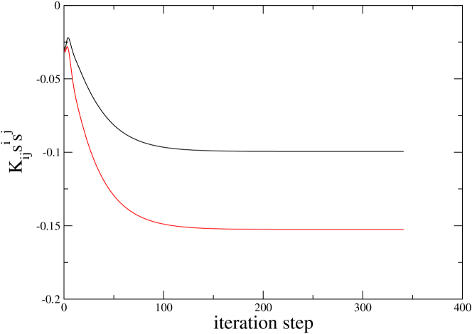
Figure 11.1: Value of $K_{ij}s^{i}s^{j}$ along the iteration of the simultaneous numerical implementation of Eqs.(11.24) and (11.29).

In brief, keeping boundary conditions in geometrical form we gain in flexibility for combining them in different manners. See Ref. [100] for other possibilities, in particular the enforcing of the vanishing of $\theta$ as a condition on the normal part of the shift, $\tilde{b}$, instead of a condition on $\Psi$. In conjunction with Eq. (11.15) for $\bm{V}$, this means that the NEH condition $\bm{\Theta}=0$ can be completely fulfilled by an appropriate choice of the shift $\bm{\beta}$.

12 Conclusion

In this article, we have developed an approach to null hypersurfaces based on the 3+1 formalism of general relativity, the main motivation being the application of the isolated horizon formalism to numerical relativity. Although the geometry of a null hypersurface ${\mathcal{H}}$ can be elegantly studied from a purely intrinsic point of view, i.e. without referring to objects defined outside ${\mathcal{H}}$, the present 3+1 strategy proves to be useful, at least for two reasons. First of all, any 3+1 spacelike slicing $(\Sigma_{t})$ provides a natural normalization of the null normal $\bm{\ell}$ to ${\mathcal{H}}$, along with a projector $\bm{\Pi}$ onto ${\mathcal{H}}$ — fixing the ambiguities inherent to null hypersurfaces. Secondly, this permits to express explicitly ${\mathcal{H}}$’s intrinsic quantities in terms of fields of direct interest for numerical relativity, like the extrinsic curvature $\bm{K}$ of the hypersurface $\Sigma_{t}$ and its the 3-metric $\bm{\gamma}$ [or its conformal representation $(\Psi,\bm{\tilde{\gamma}})$]. In addition, we have adopted a fully 4-dimensional point of view, by introducing an auxiliary null foliation $({\mathcal{H}}_{u})$ in a neighborhood of ${\mathcal{H}}$. Not only this facilitates the link between the null geometry and the 3+1 description, but also reduces the actual computations to standard 4-dimensional tensorial calculus (e.g. involving the spacetime connection $\bm{\nabla}$) and 4-dimensional exterior calculus (e.g. the differential $\bm{\mathrm{d}}\underline{\bm{\ell}}$ and $\bm{\mathrm{d}}\underline{\bm{k}}$ of 1-forms associated with the null normal $\bm{\ell}$ and the ingoing null vector $\bm{k}$, in connection with Frobenius theorem related to the submanifolds ${\mathcal{H}}$ and ${\mathcal{S}}_{t}={\mathcal{H}}\cap\Sigma_{t}$, or the decomposition of the curvature tensor following from Cartan’s structure equations).

Thanks to the projector $\bm{\Pi}$, we have performed a 4-dimensional extension of ${\mathcal{H}}$’s second fundamental form $\bm{\Theta}$, and of the Háj́iček 1-form $\bm{\Omega}$. Besides, we have introduced as a basic object the transversal deformation rate $\bm{\Xi}$. By performing various projections of the Einstein equation, we have recovered, in addition to the null Raychaudhuri equation, the Damour-Navier-Stokes equation, and have derived an evolution equation for $\bm{\Xi}$. Independently of the Einstein equation, the so-called tidal force equation (which involves the Weyl tensor) is recovered. All these equations constitute a set of evolution equations along the null generators of ${\mathcal{H}}$. They hold for any null hypersurface.

Following Háj́iček  and Ashtekar et al., we have then considered non-expanding null hypersurfaces (more specifically non-expanding horizons) as a first step in the modelisation of a black hole horizon in quasi-equilibrium. At this stage, a new geometrical structure enters into the scene, namely the connection $\bm{\hat{\nabla}}$ on ${\mathcal{H}}$ compatible with the degenerate metric $\bm{q}$ and induced by the spacetime connection $\bm{\nabla}$. This can be achieved thanks to the vanishing of the second fundamental form $\bm{\Theta}$ for a non-expanding null hypersurface. The couple $(\bm{q},\bm{\hat{\nabla}})$ then completely characterizes the geometry of a non-expanding horizon. Once the null normal $\bm{\ell}$ is fixed by some 3+1 slicing $(\Sigma_{t})$, this geometry is encoded in the fields $(\bm{q},\bm{\Omega},\kappa,\bm{\Xi})$ evaluated in a spatial cross-section ${\mathcal{S}}_{t}={\mathcal{H}}\cap\Sigma_{t}$. The change in time of these quantities is obtained by specializing the evolution equations to the case $\bm{\Theta}=0$. A number of possible constraints then follow for characterizing a horizon in quasi-equilibrium, beyond being simply non-expanding, leading to a hierarchy of structures on ${\mathcal{H}}$. In particular, an intermediate notion of quasi-equilibrium is provided by the weakly isolated horizon structure introduced by Ashtekar et al. and defined by requiring (i) a time-independent $\bm{\Omega}$ and (ii) $\kappa$ to be constant over ${\mathcal{H}}$. This permits a quasi-local expression of physical parameters, like mass and angular momentum and gives constraints on the 3+1 slicing, even if it does not further constrain the geometry of ${\mathcal{H}}$. On the contrary, the isolated horizon structure, that requires all fields $(\bm{q},\bm{\Omega},\kappa,\bm{\Xi})$ to be time-independent, represents the maximal degree of equilibrium imposed in a quasi-local manner. It really restricts ${\mathcal{H}}$ among all possible non-expanding horizons. It also provides tools for extracting information in the neighborhood of ${\mathcal{H}}$.

Thanks to explicit formulæ  relating $\bm{q}$, $\bm{\Theta}$, $\bm{\Omega}$, $\kappa$ and $\bm{\Xi}$ to 3+1 fields, including the lapse function $N$ and shift vector $\bm{\beta}$, we have then translated the isolated horizon hierarchy into inner boundary conditions onto an excised sphere in the spatial hypersurface $\Sigma_{t}$. This permits us to study the problem of initial data and spacetime evolution in a constrained scheme, making the links with existing results in for numerical relativity. This connection with the 3+1 Cauchy problem illustrates the “down-up” strategy mentioned in the Introduction, i.e. the description of the null geometry on ${\mathcal{H}}$ by constructing it from initial data on a spacelike 2-surface. This provides an alternative point of view to the “up-down” picture, generally considered in the isolated horizon literature, and in which data on spatial slices are determined a posteriori from a given 3-geometry on ${\mathcal{H}}$ as a whole. In conclusion, the tools discussed in this article are aimed to provide a useful setting for studying black holes in realistic astrophysical scenarios involving regimes close to the steady state.

Appendix A Flow of time: various Lie derivatives along $\bm{\ell}$

The choice (4.5) for $\bm{\ell}$, as the tangent vector of ${\mathcal{H}}$’s null generators associated with the parameter $t$, means that $\bm{\ell}$ can be considered as the “advance-in-time” vector associated with $t$. This is also manifest in the relation $\langle\bm{\mathrm{d}}t,\bm{\ell}\rangle=1$ [Eq. (4.6)] or $\bm{\ell}=\bm{t}+\bm{V}+(N-b)\bm{s}$ [Eq. (4.68)], which shows that $\bm{\ell}$ is equal to the coordinate time vector $\bm{t}$ plus some vector tangent to $\Sigma_{t}$ [namely $\bm{V}+(N-b)\bm{s}$]. Therefore in order to describe the “time evolution” of the objects related to ${\mathcal{H}}$, it is natural to introduce the Lie derivative along $\bm{\ell}$. However, it turns out that various kinds of such Lie derivatives can be defined. First of all, there is the Lie derivative along the vector field $\bm{\ell}$ within the spacetime manifold ${\mathcal{M}}$, which is denoted by $\bm{\mathcal{L}}_{\bm{\bm{\ell}}}\,$. But since $\bm{\ell}\in{\mathcal{T}}({\mathcal{H}})$, there is also the Lie derivative along the vector field $\bm{\ell}$ within the manifold ${\mathcal{H}}$, which we denote by ${}^{{\mathcal{H}}}\!\bm{\mathcal{L}}_{\bm{\bm{\ell}}}\,$. Finally, since $\bm{\ell}$ Lie drags the 2-surfaces ${\mathcal{S}}_{t}$ (cf. Sec. 4.2 and Fig. 4.2), one may define within the manifold ${\mathcal{S}}_{t}$ a Lie derivative “along $\bm{\ell}$”, which we denote ${}^{{\mathcal{S}}}\!\bm{\mathcal{L}}_{\bm{\bm{\ell}}}\,$. We present here the precise definitions of these Lie derivatives and the relationships between them.

A.1 Lie derivative along $\bm{\ell}$ within ${\mathcal{H}}$: ${}^{{\mathcal{H}}}\!\bm{\mathcal{L}}_{\bm{\bm{\ell}}}\,$

Since $\bm{\ell}$ is a vector field on ${\mathcal{H}}$, one may naturally construct the Lie derivative along $\bm{\ell}$ of any tensor field $\bm{T}$ on ${\mathcal{H}}$. This results in another tensor field on ${\mathcal{H}}$, which we denote by ${}^{{\mathcal{H}}}\!\bm{\mathcal{L}}_{\bm{\bm{\ell}}}\,\bm{T}$. Now, we may extend $\bm{T}$ into a tensor field on ${\mathcal{M}}$ thanks to the push-forward mapping $\Phi_{*}$ for vectors [cf. Eq. (2.4)] and the operator $\bm{\Pi}^{*}$ for linear forms [cf. Eq. (4.58)]. It is then legitimate to ask for the relation between the Lie derivative $\bm{\mathcal{L}}_{\bm{\bm{\ell}}}\,$ of this 4-dimensional extension within the manifold ${\mathcal{M}}$, and ${}^{{\mathcal{H}}}\!\bm{\mathcal{L}}_{\bm{\bm{\ell}}}\,\bm{T}$.

Firstly we notice that both Lie derivatives coincide onto vectors:

$$\framebox{$\displaystyle\forall\bm{v}\in{\mathcal{T}}({\mathcal{H}}),\quad{}^{{\mathcal{H}}}\!\bm{\mathcal{L}}_{\bm{\bm{\ell}}}\,\bm{v}=\bm{\mathcal{L}}_{\bm{\bm{\ell}}}\,\bm{v}$}.$$ (A.1)

This follows from the very definition of the Lie derivative (cf. Fig. 1.1). Let us now consider an arbitrary 1-form on ${\mathcal{H}}$: $\bm{\varpi}\in{\mathcal{T}}^{*}({\mathcal{H}})$. Then invoking the Leibnitz rule on contractions and using the property (A.1)

$$\forall\bm{v}\in{\mathcal{T}}({\mathcal{H}}),\quad\langle{}^{{\mathcal{H}}}\!\bm{\mathcal{L}}_{\bm{\bm{\ell}}}\,\bm{\varpi},\bm{v}\rangle = {}^{{\mathcal{H}}}\!\bm{\mathcal{L}}_{\bm{\bm{\ell}}}\,\langle\bm{\varpi},\bm{v}\rangle-\langle\bm{\varpi},{}^{{\mathcal{H}}}\!\bm{\mathcal{L}}_{\bm{\bm{\ell}}}\,\bm{v}\rangle$$ (A.2)

$$= \bm{\mathcal{L}}_{\bm{\bm{\ell}}}\,\langle\bm{\varpi},\bm{v}\rangle-\langle\bm{\varpi},\bm{\mathcal{L}}_{\bm{\bm{\ell}}}\,\bm{v}\rangle$$

$$= \bm{\mathcal{L}}_{\bm{\bm{\ell}}}\,\langle\bm{\Pi}^{*}\bm{\varpi},\bm{v}\rangle-\langle\bm{\Pi}^{*}\bm{\varpi},\bm{\mathcal{L}}_{\bm{\bm{\ell}}}\,\bm{v}\rangle$$

$$= \langle\bm{\mathcal{L}}_{\bm{\bm{\ell}}}\,(\bm{\Pi}^{*}\bm{\varpi}),\bm{v}\rangle.$$

We conclude that the 1-forms ${}^{{\mathcal{H}}}\!\bm{\mathcal{L}}_{\bm{\bm{\ell}}}\,\bm{\varpi}$ and $\bm{\mathcal{L}}_{\bm{\bm{\ell}}}\,(\bm{\Pi}^{*}\bm{\varpi})$ coincide on ${\mathcal{T}}({\mathcal{H}})$. Therefore their extensions to ${\mathcal{T}}({\mathcal{M}})$ provided by the projector $\bm{\Pi}$ also coincide, and we can write

$$\forall\bm{\bm{\varpi}}\in{\mathcal{T}}^{*}({\mathcal{H}}),\quad\bm{\Pi}^{*}\,{}^{{\mathcal{H}}}\!\bm{\mathcal{L}}_{\bm{\bm{\ell}}}\,\bm{\varpi}=\bm{\Pi}^{*}\bm{\mathcal{L}}_{\bm{\bm{\ell}}}\,(\bm{\Pi}^{*}\bm{\bm{\varpi}}).$$ (A.3)

By taking tensorial products, we above analysis can be extended straightforwardly to any field $\bm{A}$ of multilinear forms acting on ${\mathcal{T}}_{p}({\mathcal{H}})$, so that we get

$$\framebox{$\displaystyle\forall\bm{\bm{A}}\in{\mathcal{T}}^{*}({\mathcal{H}})^{\otimes n},\quad\bm{\Pi}^{*}\,{}^{{\mathcal{H}}}\!\bm{\mathcal{L}}_{\bm{\bm{\ell}}}\,\bm{A}=\bm{\Pi}^{*}\bm{\mathcal{L}}_{\bm{\bm{\ell}}}\,(\bm{\Pi}^{*}\bm{\bm{A}})$}.$$ (A.4)

A.2 Lie derivative along $\bm{\ell}$ within ${\mathcal{S}}_{t}$: ${}^{{\mathcal{S}}}\!\bm{\mathcal{L}}_{\bm{\bm{\ell}}}\,$

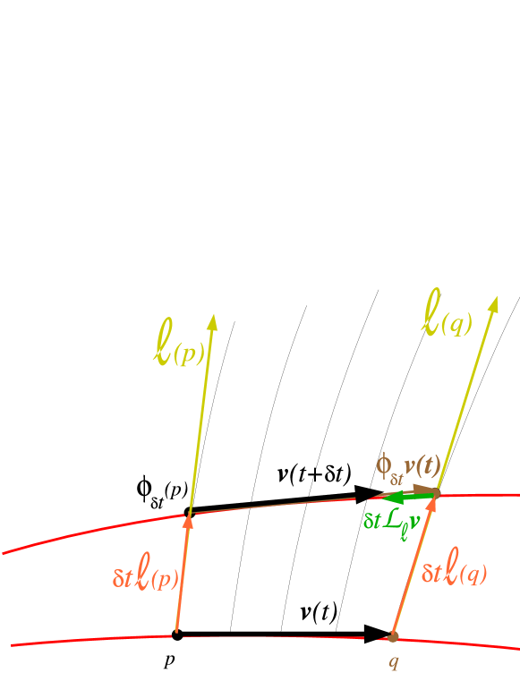
Figure 1.1: Geometrical construction showing that $\bm{\mathcal{L}}_{\bm{\bm{\ell}}}\,\bm{v}\in{\mathcal{T}}({\mathcal{S}}_{t})$ for any vector $\bm{v}$ tangent to the 2-surface ${\mathcal{S}}_{t}$: on ${\mathcal{S}}_{t}$, a vector can be identified by a infinitesimal displacement between two points, $p$ and $q$ say. These points are transported onto the neighbouring surface ${\mathcal{S}}_{t+\delta t}$ along the field lines of the vector field $\bm{\ell}$ (thin lines on the figure) by the diffeomorphism $\phi_{\delta t}$ associated with $\bm{\ell}$: the displacement between $p$ and $\phi_{\delta t}(p)$ is the vector $\delta t\,\bm{\ell}$. The couple of points $(\phi_{\delta t}(p),\phi_{\delta t}(q))$ defines the vector $\phi_{\delta t}\bm{v}(t)$ tangent to ${\mathcal{S}}_{t+\delta t}$. The Lie derivative of $\bm{v}$ along $\bm{\ell}$ is then defined by the difference between the value of the vector field $\bm{v}$ at the point $\phi_{\delta t}(p)$, i.e. $\bm{v}(t+\delta t)$, and the vector transported from ${\mathcal{S}}_{t}$ along $\bm{\ell}$’s field lines, i.e. $\phi_{\delta t}\bm{v}(t)$ : $\bm{\mathcal{L}}_{\bm{\bm{\ell}}}\,{\bm{v}}(t+\delta t)=\lim_{\delta t\rightarrow 0}[\bm{v}(t+\delta t)-\phi_{\delta t}\bm{v}(t)]/\delta t$. Since both vectors $\bm{v}(t+\delta t)$ and $\phi_{\delta t}\bm{v}(t)$ are in ${\mathcal{T}}({\mathcal{S}}_{t+\delta t})$, it is then obvious that $\bm{\mathcal{L}}_{\bm{\bm{\ell}}}\,{\bm{v}}(t+\delta t)\in{\mathcal{T}}({\mathcal{S}}_{t+\delta t})$.

We have seen in Sec. 4.2 that $\bm{\ell}$ Lie drags the 2-surfaces ${\mathcal{S}}_{t}$: ${\mathcal{S}}_{t+\delta t}$ is obtained from the neighbouring surface ${\mathcal{S}}_{t}$ by an infinitesimal displacement $\delta t\bm{\ell}$ of each point of ${\mathcal{S}}_{t}$. As stressed by Damour [60], an immediate consequence of this is that the Lie derivative along $\bm{\ell}$ of any vector tangent to ${\mathcal{S}}_{t}$ is a vector which is also tangent to ${\mathcal{S}}_{t}$:

$$\forall\bm{v}\in{\mathcal{T}}({\mathcal{S}}_{t}),\quad\bm{\mathcal{L}}_{\bm{\bm{\ell}}}\,\bm{v}\in{\mathcal{T}}({\mathcal{S}}_{t}).$$ (A.5)

This is obvious from the geometrical definition of a Lie derivative (see Fig. 1.1). It can also be established “blindly”: consider $\bm{v}\in{\mathcal{T}}({\mathcal{S}}_{t})$; then $\bm{\ell}\cdot\bm{v}=\bm{k}\cdot\bm{v}=0$, so that

$$\bm{\ell}\cdot\bm{\mathcal{L}}_{\bm{\bm{\ell}}}\,\bm{v}=\bm{\ell}\cdot(\bm{\nabla}_{\bm{\ell}}\bm{v}-\bm{\nabla}_{\bm{v}}\bm{\ell})=\underbrace{\bm{\ell}\cdot\bm{\nabla}_{\bm{\ell}}\bm{v}}_{=-\bm{v}\cdot\bm{\nabla}_{\bm{\ell}}\bm{\ell}}-\underbrace{\bm{\ell}\cdot\bm{\nabla}_{\bm{v}}\,\bm{\ell}}_{=0}=-\bm{v}\cdot(\kappa\bm{\ell})=0.$$ (A.6)

and

$$\bm{k}\cdot\bm{\mathcal{L}}_{\bm{\bm{\ell}}}\,\bm{v}=\bm{k}\cdot\bm{\nabla}_{\bm{\ell}}\bm{v}-\bm{k}\cdot\bm{\nabla}_{\bm{v}}\bm{\ell}=-\bm{v}\cdot\bm{\nabla}_{\bm{\ell}}\bm{k}+\bm{\ell}\cdot\bm{\nabla}_{\bm{v}}\bm{k}=\bm{\mathrm{d}}\underline{\bm{k}}(\bm{v},\bm{\ell}).$$ (A.7)

With the expression (5.39) of the exterior derivative of $\underline{\bm{k}}$ and the fact that $\langle\underline{\bm{\ell}},\bm{v}\rangle=0$ and $\langle\underline{\bm{\ell}},\bm{\ell}\rangle=0$, we get immediately

$$\bm{k}\cdot\bm{\mathcal{L}}_{\bm{\bm{\ell}}}\,\bm{v}=0.$$ (A.8)

Equations (A.6) and (A.8), by stating that $\bm{\mathcal{L}}_{\bm{\bm{\ell}}}\,\bm{v}$ is orthogonal to both $\bm{\ell}$ and $\bm{k}$, show that $\bm{\mathcal{L}}_{\bm{\bm{\ell}}}\,\bm{v}$ is tangent to ${\mathcal{S}}_{t}$ [cf. Eq. (4.31)], and therefore establish (A.5). The property (A.5) means that, although $\bm{\ell}\not\in{\mathcal{T}}({\mathcal{S}}_{t})$, $\bm{\mathcal{L}}_{\bm{\bm{\ell}}}\,$ can be viewed as an internal operator on the space ${\mathcal{T}}({\mathcal{S}}_{t})$ of vector fields tangent to ${\mathcal{S}}_{t}$. We will denote it as ${}^{{\mathcal{S}}}\!\bm{\mathcal{L}}_{\bm{\bm{\ell}}}\,$ to stress this feature and rewrite Eq. (A.5) as

$$\framebox{$\displaystyle\forall\bm{v}\in{\mathcal{T}}({\mathcal{S}}_{t}),\quad{}^{{\mathcal{S}}}\!\bm{\mathcal{L}}_{\bm{\bm{\ell}}}\,\bm{v}:=\bm{\mathcal{L}}_{\bm{\bm{\ell}}}\,\bm{v}\in{\mathcal{T}}({\mathcal{S}}_{t})$}.$$ (A.9)

The definition of ${}^{{\mathcal{S}}}\!\bm{\mathcal{L}}_{\bm{\bm{\ell}}}\,$ can be extended to 1-forms on ${\mathcal{S}}_{t}$ by demanding that the Leibnitz rule holds for the contraction of a 1-form and a vector field: if $\bm{\varpi}\in{\mathcal{T}}^{*}({\mathcal{S}}_{t})$ is a 1-form on ${\mathcal{S}}_{t}$, we define the Lie derivative ${}^{{\mathcal{S}}}\!\bm{\mathcal{L}}_{\bm{\bm{\ell}}}\,\bm{\varpi}$ of $\bm{\varpi}$ along $\bm{\ell}$ as the 1-form whose action on vectors is

$$\forall\bm{v}\in{\mathcal{T}}({\mathcal{S}}_{t}),\quad\langle{}^{{\mathcal{S}}}\!\bm{\mathcal{L}}_{\bm{\bm{\ell}}}\,\bm{\varpi},\bm{v}\rangle:=\bm{\mathcal{L}}_{\bm{\bm{\ell}}}\,\langle\bm{\varpi},\bm{v}\rangle-\langle\bm{\varpi},{}^{{\mathcal{S}}}\!\bm{\mathcal{L}}_{\bm{\bm{\ell}}}\,\bm{v}\rangle.$$ (A.10)

Note that the right-hand side of this equation is well defined since ${}^{{\mathcal{S}}}\!\bm{\mathcal{L}}_{\bm{\bm{\ell}}}\,\bm{v}\in{\mathcal{T}}({\mathcal{S}}_{t})$, so that we can apply the 1-form $\bm{\varpi}$ to it. We can extend the definition of the Lie derivative ${}^{{\mathcal{S}}}\!\bm{\mathcal{L}}_{\bm{\bm{\ell}}}\,$ to bilinear forms on ${\mathcal{S}}_{t}$, and more generally to multilinear forms, by means of Leibnitz rule:

$${}^{{\mathcal{S}}}\!\bm{\mathcal{L}}_{\bm{\bm{\ell}}}\,(\bm{\varpi}_{1}\otimes\bm{\varpi}_{2})={}^{{\mathcal{S}}}\!\bm{\mathcal{L}}_{\bm{\bm{\ell}}}\,\bm{\varpi}_{1}\otimes\bm{\varpi}_{2}+\bm{\varpi}_{1}\otimes{}^{{\mathcal{S}}}\!\bm{\mathcal{L}}_{\bm{\bm{\ell}}}\,\bm{\varpi}_{2}.$$ (A.11)

Taking into account the property (A.9), which also holds for any tensorial product of vectors, we finally conclude that the Lie derivative operator ${}^{{\mathcal{S}}}\!\bm{\mathcal{L}}_{\bm{\bm{\ell}}}\,$ is defined for any tensor field on ${\mathcal{S}}_{t}$: it is internal to ${\mathcal{S}}_{t}$ in the sense that it transforms a tensor field on ${\mathcal{S}}_{t}$ into another tensor field on ${\mathcal{S}}_{t}$. This 2-dimensional operator has been introduced by Damour [60, 61] and called by him the “convective derivative”.

Now, any 1-form $\bm{\varpi}\in{\mathcal{T}}^{*}({\mathcal{S}}_{t})$ can also be seen as a 1-form on ${\mathcal{M}}$ thanks to the orthogonal projector $\vec{\bm{q}}$ on ${\mathcal{T}}({\mathcal{S}}_{t})$ : it is the 1-form $\vec{\bm{q}}^{*}\bm{\varpi}$ defined by Eq. (5.11) . Let us then investigate the relation between the “4-dimensional” Lie derivative $\bm{\mathcal{L}}_{\bm{\bm{\ell}}}\,\vec{\bm{q}}^{*}\bm{\varpi}$ and the “2-dimensional” one, ${}^{{\mathcal{S}}}\!\bm{\mathcal{L}}_{\bm{\bm{\ell}}}\,\bm{\varpi}$. The first thing to notice is that the 1-forms $\bm{\mathcal{L}}_{\bm{\bm{\ell}}}\,\vec{\bm{q}}^{*}\bm{\varpi}$ and $\vec{\bm{q}}^{*}\;{}^{{\mathcal{S}}}\!\bm{\mathcal{L}}_{\bm{\bm{\ell}}}\,\bm{\varpi}$ coincide when restricted to ${\mathcal{T}}({\mathcal{S}}_{t})$. Indeed

$$\forall\bm{v}\in{\mathcal{T}}({\mathcal{S}}_{t}),\quad\langle\bm{\mathcal{L}}_{\bm{\bm{\ell}}}\,\vec{\bm{q}}^{*}\bm{\varpi},\bm{v}\rangle = \bm{\mathcal{L}}_{\bm{\bm{\ell}}}\,\langle\vec{\bm{q}}^{*}\bm{\varpi},\bm{v}\rangle-\langle\vec{\bm{q}}^{*}\bm{\varpi},\bm{\mathcal{L}}_{\bm{\bm{\ell}}}\,\bm{v}\rangle$$ (A.12)

$$= \bm{\mathcal{L}}_{\bm{\bm{\ell}}}\,\langle\bm{\varpi},\vec{\bm{q}}(\bm{v})\rangle-\langle\bm{\varpi},\vec{\bm{q}}(\bm{\mathcal{L}}_{\bm{\bm{\ell}}}\,\bm{v})\rangle$$

$$= \bm{\mathcal{L}}_{\bm{\bm{\ell}}}\,\langle\bm{\varpi},\bm{v}\rangle-\langle\bm{\varpi},\bm{\mathcal{L}}_{\bm{\bm{\ell}}}\,\bm{v}\rangle$$

$$= \langle{}^{{\mathcal{S}}}\!\bm{\mathcal{L}}_{\bm{\bm{\ell}}}\,\bm{\varpi},\bm{v}\rangle,$$

where the third equality follows from property (A.5) and the fourth one from the definition (A.10). Hence

$$\forall\bm{\varpi}\in{\mathcal{T}}^{*}({\mathcal{S}}_{t}),\quad{}^{{\mathcal{S}}}\!\bm{\mathcal{L}}_{\bm{\bm{\ell}}}\,\bm{\varpi}=\left.\left(\bm{\mathcal{L}}_{\bm{\bm{\ell}}}\,\vec{\bm{q}}^{*}\bm{\varpi}\right)\right|_{{\mathcal{T}}({\mathcal{S}}_{t})}.$$ (A.13)

Moreover,

$$\forall\bm{\varpi}\in{\mathcal{T}}^{*}({\mathcal{S}}_{t}),\quad\langle\bm{\mathcal{L}}_{\bm{\bm{\ell}}}\,\vec{\bm{q}}^{*}\bm{\varpi},\bm{\ell}\rangle = \bm{\mathcal{L}}_{\bm{\bm{\ell}}}\,\underbrace{\langle\vec{\bm{q}}^{*}\bm{\varpi},\bm{\ell}\rangle}_{=0}-\langle\vec{\bm{q}}^{*}\bm{\varpi},\underbrace{\bm{\mathcal{L}}_{\bm{\bm{\ell}}}\,\bm{\ell}}_{=0}\rangle$$

$$\langle\bm{\mathcal{L}}_{\bm{\bm{\ell}}}\,\vec{\bm{q}}^{*}\bm{\varpi},\bm{\ell}\rangle = 0.$$ (A.14)

Since $\langle\vec{\bm{q}}^{*}\;{}^{{\mathcal{S}}}\!\bm{\mathcal{L}}_{\bm{\bm{\ell}}}\,\bm{\varpi},\bm{\ell}\rangle=0$ (for $\vec{\bm{q}}(\bm{\ell})=0$), we can combine Eqs. (A.13) and (A.14) in

$$\forall\bm{\varpi}\in{\mathcal{T}}^{*}({\mathcal{S}}_{t}),\quad\left.\left(\vec{\bm{q}}^{*}\;{}^{{\mathcal{S}}}\!\bm{\mathcal{L}}_{\bm{\bm{\ell}}}\,\bm{\varpi}\right)\right|_{{\mathcal{T}}({\mathcal{H}})}=\left.\left(\bm{\mathcal{L}}_{\bm{\bm{\ell}}}\,\vec{\bm{q}}^{*}\bm{\varpi}\right)\right|_{{\mathcal{T}}({\mathcal{H}})}.$$ (A.15)

But regarding the direction transverse to ${\mathcal{H}}$ one has

$$\forall\bm{\varpi}\in{\mathcal{T}}^{*}({\mathcal{S}}_{t}),\quad\langle\bm{\mathcal{L}}_{\bm{\bm{\ell}}}\,\vec{\bm{q}}^{*}\bm{\varpi},\bm{k}\rangle = \bm{\mathcal{L}}_{\bm{\bm{\ell}}}\,\underbrace{\langle\vec{\bm{q}}^{*}\bm{\varpi},\bm{k}\rangle}_{=0}-\langle\vec{\bm{q}}^{*}\bm{\varpi},\underbrace{\bm{\mathcal{L}}_{\bm{\bm{\ell}}}\,\bm{k}}_{=[\bm{\ell},\bm{k}]}\rangle$$

$$\langle\bm{\mathcal{L}}_{\bm{\bm{\ell}}}\,\vec{\bm{q}}^{*}\bm{\varpi},\bm{k}\rangle = \langle\bm{\varpi},\vec{\bm{q}}([\bm{k},\bm{\ell}])\rangle,$$ (A.16)

where $[\bm{k},\bm{\ell}]$ denotes the commutator of vectors $\bm{k}$ and $\bm{\ell}$. The right-hand side of Eq. (A.16) is in general different from zero. Indeed, a simple calculation using Eq. (5.39) shows that

$$[k,\ell]^{\alpha}=k^{\mu}(\nabla_{\mu}\ell^{\alpha}+\nabla^{\alpha}\ell_{\mu})-\frac{1}{2N^{2}}\nabla_{\bm{\ell}}\ln\left(\frac{N}{M}\right)\,\ell^{\alpha},$$ (A.17)

so that

$$q^{\alpha}_{\ \,\mu}[k,\ell]^{\mu}=k^{\mu}q^{\alpha\nu}(\nabla_{\mu}\ell_{\nu}+\nabla_{\nu}\ell_{\mu}).$$ (A.18)

For instance a sufficient condition for the right-hand side of Eq. (A.16) to vanish, and then $\bm{\mathcal{L}}_{\bm{\bm{\ell}}}\,\vec{\bm{q}}^{*}\bm{\varpi}$ to coincide with $\vec{\bm{q}}^{*}{}^{{\mathcal{S}}}\!\bm{\mathcal{L}}_{\bm{\bm{\ell}}}\,\bm{\varpi}$, consists in demanding $\bm{\ell}$ to be a Killing vector of spacetime: $\nabla_{\alpha}\ell_{\beta}+\nabla_{\beta}\ell_{\alpha}=0$.

Another writing of Eq. (A.13) is

$$\forall\bm{\varpi}\in{\mathcal{T}}^{*}({\mathcal{S}}_{t}),\quad\vec{\bm{q}}^{*}\;{}^{{\mathcal{S}}}\!\bm{\mathcal{L}}_{\bm{\bm{\ell}}}\,\bm{\varpi}=\vec{\bm{q}}^{*}\bm{\mathcal{L}}_{\bm{\bm{\ell}}}\,\vec{\bm{q}}^{*}\bm{\varpi},$$ (A.19)

where each side of the equality is a 1-form on ${\mathcal{T}}({\mathcal{M}})$ and the operators $\vec{\bm{q}}^{*}$ added with respect to Eq. (A.13) effectively restrict the non-trivial action of these 1-forms to the subspace ${\mathcal{T}}({\mathcal{S}}_{t})$ of ${\mathcal{T}}({\mathcal{M}})$.

By taking tensorial products, the above analysis can be extended easily to any multilinear form $\bm{A}$ acting on ${\mathcal{T}}({\mathcal{S}}_{t})$. In particular Eq. (A.19) can be generalized to

$$\framebox{$\displaystyle\forall\bm{A}\in{\mathcal{T}}^{*}({\mathcal{S}}_{t})^{\otimes n},\quad\vec{\bm{q}}^{*}\;{}^{{\mathcal{S}}}\!\bm{\mathcal{L}}_{\bm{\bm{\ell}}}\,\bm{A}=\vec{\bm{q}}^{*}\bm{\mathcal{L}}_{\bm{\bm{\ell}}}\,\vec{\bm{q}}^{*}\bm{A}$}.$$ (A.20)

Note the similarity between this relation and Eq. (A.4) for ${}^{{\mathcal{H}}}\!\bm{\mathcal{L}}_{\bm{\bm{\ell}}}\,$.

Appendix B Cartan’s structure equations

Many studies about null hypersurfaces and isolated horizons make use of the Newman-Penrose framework, which is based on the complex null tetrad introduced in Sec. 4.6. An alternative approach is Cartan’s formalism which is based on a real tetrad and exterior calculus (see e.g. Chap. 14 of MTW [123] or Chap. V.B of Ref. [46] for an introduction). Cartan’s formalism is at least as powerful as the Newman-Penrose one, although it remains true that the latter is well adapted to null surfaces.

B.1 Tetrad and connection 1-forms

In the present context, it is natural to consider the following bases for, respectively, ${\mathcal{T}}({\mathcal{M}})$ (vector fields) and ${\mathcal{T}}^{*}({\mathcal{M}})$ (1-forms)

$$\bm{e}_{\alpha}=(\bm{\ell},\bm{k},\bm{e}_{2},\bm{e}_{3})\quad\mbox{and}\quad\bm{e}^{\alpha}=(-\underline{\bm{k}},-\underline{\bm{\ell}},\bm{e}^{2},\bm{e}^{3}),$$ (B.1)

where $\bm{e}_{2}$ and $\bm{e}_{3}$ are two vector fields tangent to the 2-surface ${\mathcal{S}}_{t}$ which constitute an orthonormal basis of ${\mathcal{T}}({\mathcal{S}}_{t})$ (with respect to the induced Riemannian metric $\bm{q}$ of ${\mathcal{S}}_{t}$) and $\bm{e}^{2}$ and $\bm{e}^{3}$ are the two 1-forms in ${\mathcal{T}}^{*}({\mathcal{M}})$ such that the basis $(\bm{e}^{\alpha})$ of ${\mathcal{T}}^{*}({\mathcal{M}})$ is the dual of the basis $(\bm{e}_{\alpha})$ of ${\mathcal{T}}({\mathcal{M}})$, i.e. it satisfies

$$\langle\bm{e}^{\alpha},\bm{e}_{\beta}\rangle=\delta^{\alpha}_{\ \,\beta},$$ (B.2)

where $\delta^{\alpha}_{\ \,\beta}$ denotes the Kronecker symbol. The vector basis $(\bm{e}_{\alpha})$ is usually called a tetrad, or moving frame or repère mobile. Note that the ordering $(\bm{e}_{0}=\bm{\ell},\;\bm{e}_{1}=\bm{k})$ and $(\bm{e}^{0}=-\underline{\bm{k}},\;\bm{e}^{1}=-\underline{\bm{\ell}})$ has been chosen to ensure Eq. (B.2) for $\alpha,\beta\in\{0,1\}$, by virtue of the fact that $\bm{\ell}$ and $\bm{k}$ are null vectors and satisfy $\bm{\ell}\cdot\bm{k}=-1$ [Eq. (4.28)]. Note that the tetrad $(\bm{\ell},\bm{k},\bm{e}_{2},\bm{e}_{3})$ is the same as that used to construct the complex Newman-Penrose null tetrad in Sec. 4.6.

Thanks to the properties (4.28) and (4.31), the metric tensor components with respect to the chosen tetrad are

$$g_{\alpha\beta}=\bm{g}(\bm{e}_{\alpha},\bm{e}_{\beta})=\left(\begin{array}[]{cccc}0&-1&\ \,0&\ \,0\\ -1&0&\ \,0&\ \,0\\ 0&0&\ \,1&\ \,0\\ 0&0&\ \,0&\ \,1\end{array}\right).$$ (B.3)

The connection 1-forms of the spacetime connection $\bm{\nabla}$ with respect to the tetrad $(\bm{e}_{\alpha})$ are the sixteen 1-forms $\bm{\omega}^{\beta}_{\ \,\alpha}$ defined by

$$\forall\bm{v}\in{\mathcal{T}}({\mathcal{M}}),\quad\bm{\nabla}_{\bm{v}}\,\bm{e}_{\alpha}=\langle\bm{\omega}^{\mu}_{\ \,\alpha},\bm{v}\rangle\,\bm{e}_{\mu}.$$ (B.4)

The expansions of the connection 1-forms on the basis $(\bm{e}^{\alpha})$ of ${\mathcal{T}}^{*}({\mathcal{M}})$ define the connection coefficients $\Gamma^{\beta}_{\ \,\alpha\gamma}$ of $\bm{\nabla}$ with respect to the tetrad $(\bm{e}_{\alpha})$:

$$\bm{\omega}^{\beta}_{\ \,\alpha}=\Gamma^{\beta}_{\ \,\alpha\mu}\,\bm{e}^{\mu}\qquad\mbox{or}\qquad\Gamma^{\beta}_{\ \,\alpha\gamma}=\langle\bm{e}^{\beta},\bm{\nabla}_{\bm{e}_{\gamma}}\bm{e}_{\alpha}\rangle.$$ (B.5)

By direct computations using the formulas of Sec. 5, we get

$$\bm{\omega}^{0}_{\ \,0}=-\bm{\omega}^{1}_{\ \,1}=\bm{\omega}-N^{-2}\bm{\nabla}_{\bm{\ell}}\sigma\,\underline{\bm{\ell}}$$ (B.6)

$$\bm{\omega}^{1}_{\ \,0}=\bm{\omega}^{0}_{\ \,1}=0$$ (B.7)

$$\bm{\omega}^{a}_{\ \,0}=\bm{\omega}^{1}_{\ \,a}=(\Omega_{a}-\bm{\nabla}_{\bm{e}_{a}}\rho)\,\underline{\bm{\ell}}+\Theta_{ab}\,\bm{e}^{b}$$ (B.8)

$$\bm{\omega}^{a}_{\ \,1}=\bm{\omega}^{0}_{\ \,a}=-\Omega_{a}\,\underline{\bm{k}}-N^{-2}\bm{\nabla}_{\bm{e}_{a}}\sigma\,\underline{\bm{\ell}}+\Xi_{ab}\,\bm{e}^{b}$$ (B.9)

$$\bm{\omega}^{b}_{\ \,a}=-\bm{\omega}^{a}_{\ \,b}=-\Gamma^{b}_{\ \,a0}\,\underline{\bm{k}}-\Gamma^{b}_{\ \,a1}\,\underline{\bm{\ell}}+\Gamma^{b}_{\ \,ac}\,\bm{e}^{c},$$ (B.10)

where $\rho$ is related to the lapse $N$ and the metric factor $M$ by $\rho=\ln(MN)$ [Eq. (4.17)] and we have introduced the abbreviation

$$\sigma:=\frac{1}{2}\ln\left(\frac{N}{M}\right).$$ (B.11)

$\Omega_{a}$, $\Theta_{ab}$ and $\Xi_{ab}$ denote the components of respectively the Háj́iček 1-form $\bm{\Omega}$, the deformation rate $\bm{\Theta}$ and transversal deformation rate $\bm{\Xi}$ with respect to the basis $(\bm{e}^{a})=(\bm{e}^{2},\bm{e}^{3})$ of ${\mathcal{T}}^{*}({\mathcal{S}}_{t})$:

$$\bm{\Omega}=\Omega_{a}\,\bm{e}^{a},\quad\bm{\Theta}=\Theta_{ab}\,\bm{e}^{a}\otimes\bm{e}^{b}\quad\mbox{and}\quad\bm{\Xi}=\Xi_{ab}\,\bm{e}^{a}\otimes\bm{e}^{b}.$$ (B.12)

Note that the above expressions are not restricted to ${\mathcal{T}}({\mathcal{S}}_{t})$ but do constitute 4-dimensional writings of the 1-form $\bm{\Omega}$ and the bilinear forms $\bm{\Theta}$ and $\bm{\Xi}$, since all these forms vanish on the vectors $\bm{e}_{0}=\bm{\ell}$ and $\bm{e}_{1}=\bm{k}$ [cf. Eqs. (5.14), (5.33), and (5.80)]. Note also that since the basis $(\bm{e}_{a})$ is orthonormal, one has $\Theta^{a}_{\ \,b}=\Theta_{ab}$ and $\Xi^{a}_{\ \,b}=\Xi_{ab}$.

The symmetries (or antisymmetries) of the 1-forms $\bm{\omega}^{\beta}_{\ \,\alpha}$ when changing the indices $\alpha$ and $\beta$, as expressed in Eqs. (B.6)-(B.10), are due to the constancy of the components $g_{\alpha\beta}$ of the metric tensor $\bm{g}$ in the basis $\bm{e}^{\alpha}\otimes\bm{e}^{\beta}$ [cf. Eq. (B.3)]. Indeed this constancy, altogether with the metric compatibility relation $\bm{\mathrm{d}}g_{\alpha\beta}=\bm{\omega}_{\alpha\beta}+\bm{\omega}_{\beta\alpha}$ (cf. e.g. Eq. (14.31b) of MTW [123]), implies $\bm{\omega}_{\alpha\beta}=-\bm{\omega}_{\beta\alpha}$, where $\bm{\omega}_{\alpha\beta}:=g_{\alpha\mu}\bm{\omega}^{\mu}_{\ \,\beta}$. In particular $\bm{\omega}^{2}_{\ \,2}=\bm{\omega}^{3}_{\ \,3}=0$.

B.2 Cartan’s first structure equation

Cartan’s first structure equation states that the exterior derivative of each 1-form $\bm{e}^{\alpha}$ is a 2-form which is expressible as a sum of exterior products involving the connection 1-forms:

$$\bm{\mathrm{d}}\bm{e}^{\alpha}=\bm{e}^{\mu}\wedge\bm{\omega}^{\alpha}_{\ \,\mu}.$$ (B.13)

These relations actually express the vanishing of the torsion of the spacetime connection $\bm{\nabla}$.

For $\alpha=0$, Eq. (B.13) results in

$$\bm{\mathrm{d}}\bm{e}^{0} = \bm{e}^{0}\wedge\bm{\omega}^{0}_{\ \,0}+\bm{e}^{1}\wedge\bm{\omega}^{0}_{\ \,1}+\bm{e}^{a}\wedge\bm{\omega}^{0}_{\ \,a}$$

$$-\bm{\mathrm{d}}\underline{\bm{k}} = -\underline{\bm{k}}\wedge(\bm{\omega}-N^{-2}\bm{\nabla}_{\bm{\ell}}\sigma\,\underline{\bm{\ell}})+\bm{e}^{a}\wedge(-\Omega_{a}\,\underline{\bm{k}}-N^{-2}\bm{\nabla}_{\bm{e}_{a}}\sigma\,\underline{\bm{\ell}}+\Xi_{ab}\,\bm{e}^{b})$$

$$\bm{\mathrm{d}}\underline{\bm{k}} = \underline{\bm{k}}\wedge\bm{\omega}-N^{-2}\bm{\nabla}_{\bm{\ell}}\sigma\,\underline{\bm{k}}\wedge\underline{\bm{\ell}}+\underbrace{\Omega_{a}\bm{e}^{a}}_{=\bm{\Omega}}\wedge\underline{\bm{k}}+N^{-2}\bm{\nabla}_{\bm{e}_{a}}\sigma\,\bm{e}^{a}\wedge\underline{\bm{\ell}}$$

$$-\underbrace{\Xi_{ab}\,\bm{e}^{a}\wedge\bm{e}^{b}}_{=0}$$

$$= \underline{\bm{k}}\wedge(\bm{\Omega}-\kappa\underline{\bm{k}})-\underline{\bm{k}}\wedge\bm{\Omega}+N^{-2}\left(-\bm{\nabla}_{\bm{\ell}}\sigma\,\underline{\bm{k}}+\bm{\nabla}_{\bm{e}_{a}}\sigma\,\bm{e}^{a}\right)\wedge\underline{\bm{\ell}}$$

$$= N^{-2}\left(-\bm{\nabla}_{\bm{k}}\sigma\,\underline{\bm{\ell}}-\bm{\nabla}_{\bm{\ell}}\sigma\,\underline{\bm{k}}+\bm{\nabla}_{\bm{e}_{a}}\sigma\,\bm{e}^{a}\right)\wedge\underline{\bm{\ell}}$$

$$\bm{\mathrm{d}}\underline{\bm{k}} = N^{-2}\bm{\mathrm{d}}\sigma\wedge\underline{\bm{\ell}},$$ (B.14)

where we have used the symmetry of $\Xi_{ab}$, as well as the expression (5.35) of $\bm{\omega}$ in terms of $\bm{\Omega}$ and $\underline{\bm{k}}$. Equation (B.14) is nothing but the Frobenius relation (5.39).

For $\alpha=1$, Eq. (B.13) results in

$$\bm{\mathrm{d}}\bm{e}^{1} = \bm{e}^{0}\wedge\bm{\omega}^{1}_{\ \,0}+\bm{e}^{1}\wedge\bm{\omega}^{1}_{\ \,1}+\bm{e}^{a}\wedge\bm{\omega}^{1}_{\ \,a}$$

$$-\bm{\mathrm{d}}\underline{\bm{\ell}} = -\underline{\bm{\ell}}\wedge(-\bm{\omega}+N^{-2}\bm{\nabla}_{\bm{\ell}}\sigma\,\underline{\bm{\ell}})+\bm{e}^{a}\wedge\left[(\Omega_{a}-\bm{\nabla}_{\bm{e}_{a}}\rho)\,\underline{\bm{\ell}}+\Theta_{ab}\,\bm{e}^{b}\right]$$

$$\bm{\mathrm{d}}\underline{\bm{\ell}} = (\bm{\omega}-\bm{\Omega}+\bm{e}^{a}\bm{\nabla}_{\bm{e}_{a}}\rho)\wedge\underline{\bm{\ell}}-\underbrace{\Theta_{ab}\,\bm{e}^{a}\wedge\bm{e}^{b}}_{=0}=(-\kappa\,\underline{\bm{k}}+\bm{e}^{a}\bm{\nabla}_{\bm{e}_{a}}\rho)\wedge\underline{\bm{\ell}}$$

$$= (-\bm{\nabla}_{\bm{\ell}}\,\rho\,\underline{\bm{k}}-\bm{\nabla}_{\bm{k}}\,\rho\,\underline{\bm{\ell}}+\bm{\nabla}_{\bm{e}_{a}}\rho\,\bm{e}^{a})\wedge\underline{\bm{\ell}}$$

$$\bm{\mathrm{d}}\underline{\bm{\ell}} = \bm{\mathrm{d}}\rho\wedge\underline{\bm{\ell}},$$ (B.15)

where we have used the symmetry of $\Theta_{ab}$, as well as Eqs. (5.35) and (2.22). Again, we recover a previously derived Frobenius relation, namely Eq. (2.17).

Finally, for $\alpha=a=2$ or $3$, Cartan’s first structure equation (B.13) results in

$$\bm{\mathrm{d}}\bm{e}^{a} = \bm{e}^{0}\wedge\bm{\omega}^{a}_{\ \,0}+\bm{e}^{1}\wedge\bm{\omega}^{a}_{\ \,1}+\bm{e}^{b}\wedge\bm{\omega}^{a}_{\ \,b}$$

$$= -\underline{\bm{k}}\wedge\left[(\Omega_{a}-\bm{\nabla}_{\bm{e}_{a}}\rho)\,\underline{\bm{\ell}}+\Theta_{ab}\,\bm{e}^{b}\right]-\underline{\bm{\ell}}\wedge(-\Omega_{a}\,\underline{\bm{k}}-N^{-2}\bm{\nabla}_{\bm{e}_{a}}\sigma\,\underline{\bm{\ell}}+\Xi_{ab}\,\bm{e}^{b})$$

$$+\bm{e}^{b}\wedge\left(-\Gamma^{a}_{\ \,b0}\,\underline{\bm{k}}-\Gamma^{a}_{\ \,b1}\,\underline{\bm{\ell}}+\Gamma^{a}_{\ \,bc}\,\bm{e}^{c}\right)$$

$$\bm{\mathrm{d}}\bm{e}^{a} = \left(2\Omega_{a}-\bm{\nabla}_{\bm{e}_{a}}\rho\right)\underline{\bm{\ell}}\wedge\underline{\bm{k}}+\left(\Theta_{ab}-\Gamma^{a}_{\ \,b0}\right)\bm{e}^{b}\wedge\underline{\bm{k}}+\left(\Xi_{ab}-\Gamma^{a}_{\ \,b1}\right)\bm{e}^{b}\wedge\underline{\bm{\ell}}$$ (B.16)

$$+\Gamma^{a}_{\ \,bc}\,\bm{e}^{b}\wedge\bm{e}^{c}.$$

B.3 Cartan’s second structure equation

Cartan’s second structure equation relates the exterior derivative of the connection 1-forms $\bm{\omega}^{\alpha}_{\ \,\beta}$ to the connection curvature:

$$\bm{\mathrm{d}}\bm{\omega}^{\alpha}_{\ \,\beta}=\bm{{\mathcal{R}}}^{\alpha}_{\ \,\beta}-\bm{\omega}^{\alpha}_{\ \,\mu}\wedge\bm{\omega}^{\mu}_{\ \,\beta},$$ (B.17)

where the $\bm{{\mathcal{R}}}^{\alpha}_{\ \,\beta}$ are the sixteen curvature 2-forms associated with the connection $\bm{\nabla}$ and the tetrad $(\bm{e}_{\alpha})$. They are defined in terms of the spacetime Riemann curvature tensor (cf. Sec. 1.2.2) by

$$\forall(\bm{u},\bm{v})\in{\mathcal{T}}({\mathcal{M}})\times{\mathcal{T}}({\mathcal{M}}),\quad\bm{{\mathcal{R}}}^{\alpha}_{\ \,\beta}(\bm{u},\bm{v}):=\mathrm{\bf Riem}(\bm{e}^{\alpha},\bm{e}_{\beta},\bm{u},\bm{v}).$$ (B.18)

Note that due to the symmetry property (1.15) of the Riemann tensor, there are actually only 6, and not 16, independent curvature 2-forms. From Eq. (B.18), the curvature 2-forms can be expressed in terms of the components $R^{\alpha}_{\ \,\beta\gamma\delta}$ of the Riemann tensor with respect to the bases $(\bm{e}_{\alpha})$ and $(\bm{e}^{\alpha})$ [cf. Eq. (1.13)] as

$$\bm{{\mathcal{R}}}^{\alpha}_{\ \,\beta}=R^{\alpha}_{\ \,\beta\mu\nu}\,\bm{e}^{\mu}\otimes\bm{e}^{\nu}=\frac{1}{2}R^{\alpha}_{\ \,\beta\mu\nu}\,\bm{e}^{\mu}\wedge\bm{e}^{\nu},$$ (B.19)

where the second equality follows from the antisymmetry of the Riemann tensor with respect to its last two indices; it clearly exhibits that $\bm{{\mathcal{R}}}^{\alpha}_{\ \,\beta}$ is a 2-form. Conversely, one may express the Riemann tensor in terms of the curvature 2-forms as

$$\mathrm{\bf Riem}=\bm{e}_{\mu}\otimes\bm{e}^{\nu}\otimes\bm{{\mathcal{R}}}^{\mu}_{\ \,\nu}.$$ (B.20)

For $\alpha=\beta=0$, Cartan’s second structure equation (B.17) results in

$$\bm{\mathrm{d}}\bm{\omega}^{0}_{\ \,0}=\bm{{\mathcal{R}}}^{0}_{\ \,0}-\bm{\omega}^{0}_{\ \,1}\wedge\bm{\omega}^{1}_{\ \,0}-\bm{\omega}^{0}_{\ \,a}\wedge\bm{\omega}^{a}_{\ \,0}$$

$$\bm{\mathrm{d}}\left(\bm{\omega}-N^{-2}\bm{\nabla}_{\bm{\ell}}\sigma\,\underline{\bm{\ell}}\right)=\bm{{\mathcal{R}}}^{0}_{\ \,0}-\left(-\Omega_{a}\,\underline{\bm{k}}-N^{-2}\bm{\nabla}_{\bm{e}_{a}}\sigma\,\underline{\bm{\ell}}+\Xi_{ab}\,\bm{e}^{b}\right)\wedge$$

$$\qquad\qquad\qquad\qquad\qquad\qquad\quad\left[(\Omega_{a}-\bm{\nabla}_{\bm{e}_{a}}\rho)\,\underline{\bm{\ell}}+\Theta_{ab}\,\bm{e}^{b}\right],$$ (B.21)

where, according to the definition (B.18) and to the symmetry property (1.15) of the Riemann tensor,

$$\bm{{\mathcal{R}}}^{0}_{\ \,0}=\mathrm{\bf Riem}(\bm{e}^{0},\bm{e}_{0},.,.)=\mathrm{\bf Riem}(-\underline{\bm{k}},\bm{\ell},.,.)=\mathrm{\bf Riem}(\underline{\bm{\ell}},\bm{k},.,.).$$ (B.22)

Expanding Eq. (B.21) [cf. Eq. (1.22)] and using Eq. (B.15) leads to

$$\bm{\mathrm{d}}\bm{\omega} = \mathrm{\bf Riem}(\underline{\bm{\ell}},\bm{k},.,.)-\Omega_{b}\Theta^{b}_{\ \,a}\,\bm{e}^{a}\wedge\underline{\bm{k}}+\Theta_{ac}\Xi^{c}_{\ \,b}\,\bm{e}^{a}\wedge\bm{e}^{b}$$ (B.23)

$$+\bigg{\{}\ \bm{\mathrm{d}}(N^{-2}\bm{\nabla}_{\bm{\ell}}\sigma)+N^{-2}\bm{\nabla}_{\bm{\ell}}\sigma\,\bm{\mathrm{d}}\rho+\Omega^{a}(\Omega_{a}-\bm{\nabla}_{\bm{e}_{a}}\rho)\,\underline{\bm{k}}$$

$$\qquad-\left[N^{-2}\bm{\nabla}_{\bm{e}_{b}}\sigma\Theta^{b}_{\ \,a}+(\Omega_{b}-\bm{\nabla}_{\bm{e}_{b}}\rho)\Xi^{b}_{\ \,a}\right]\bm{e}^{a}\ \bigg{\}}\wedge\underline{\bm{\ell}}.$$

For $\alpha=0$ and $\beta=1$ (or $\alpha=1$ and $\beta=0$), Cartan’s second structure equation (B.17) results in the trivial equation $0=0$. For $\alpha=0$ and $\beta=a$ it gives

$$\bm{\mathrm{d}}\bm{\omega}^{0}_{\ \,a}=\bm{{\mathcal{R}}}^{0}_{\ \,a}-\bm{\omega}^{0}_{\ \,0}\wedge\bm{\omega}^{0}_{\ \,a}-\bm{\omega}^{0}_{\ \,1}\wedge\bm{\omega}^{1}_{\ \,a}-\bm{\omega}^{0}_{\ \,b}\wedge\bm{\omega}^{b}_{\ \,a}$$

$$\bm{\mathrm{d}}\left(-\Omega_{a}\,\underline{\bm{k}}-N^{-2}\bm{\nabla}_{\bm{e}_{a}}\sigma\,\underline{\bm{\ell}}+\Xi_{ab}\,\bm{e}^{b}\right)=\bm{{\mathcal{R}}}^{0}_{\ \,a}$$

$$\qquad-\left(\bm{\omega}-N^{-2}\bm{\nabla}_{\bm{\ell}}\sigma\,\underline{\bm{\ell}}\right)\wedge\left(-\Omega_{a}\,\underline{\bm{k}}-N^{-2}\bm{\nabla}_{\bm{e}_{a}}\sigma\,\underline{\bm{\ell}}+\Xi_{ab}\,\bm{e}^{b}\right)$$

$$\quad+\left(\Omega_{b}\,\underline{\bm{k}}+N^{-2}\bm{\nabla}_{\bm{e}_{b}}\sigma\,\underline{\bm{\ell}}-\Xi_{bc}\,\bm{e}^{c}\right)\wedge\left(-\Gamma^{b}_{\ \,a0}\,\underline{\bm{k}}-\Gamma^{b}_{\ \,a1}\,\underline{\bm{\ell}}+\Gamma^{b}_{\ \,ad}\,\bm{e}^{d}\right).$$

Expanding this expression and using Eqs. (B.14) and (B.15), as well as $\bm{{\mathcal{R}}}^{0}_{\ \,a}=-\mathrm{\bf Riem}(\underline{\bm{k}},\bm{e}_{a},.,.)$, leads to

$$\bm{\mathrm{d}}(\Xi_{ab}\bm{e}^{b}) = -\mathrm{\bf Riem}(\underline{\bm{k}},\bm{e}_{a},.,.)+\bigg{\{}N^{-2}\left(\Omega_{a}\bm{\mathrm{d}}\sigma+\bm{\nabla}_{\bm{e}_{a}}\sigma\,\bm{\mathrm{d}}\rho+\bm{\nabla}_{\bm{e}_{a}}\sigma\,\bm{\omega}\right)$$ (B.25)

$$+\bm{\mathrm{d}}(N^{-2}\bm{\nabla}_{\bm{e}_{a}}\sigma)+\bigg{[}N^{-2}\left(\Omega_{a}\bm{\nabla}_{\bm{\ell}}\sigma+\bm{\nabla}_{\bm{e}_{b}}\sigma\Gamma^{b}_{\ \,a0}\right)-\Omega_{b}\Gamma^{b}_{\ \,a1}\bigg{]}\underline{\bm{k}}$$

$$+\bigg{[}\Xi_{bc}\Gamma^{c}_{\ \,a1}-N^{-2}\left(\Xi_{ab}\bm{\nabla}_{\bm{\ell}}\sigma+\Gamma^{c}_{\ \,ab}\bm{\nabla}_{\bm{e}_{c}}\sigma\right)\bigg{]}\bm{e}^{b}\bigg{\}}\wedge\underline{\bm{\ell}}$$

$$+\left[\bm{\mathrm{d}}\Omega_{a}+\Omega_{a}\bm{\omega}+\left(\Xi_{bc}\Gamma^{c}_{\ \,a0}-\Omega_{c}\Gamma^{c}_{\ \,ab}\right)\bm{e}^{b}\right]\wedge\underline{\bm{k}}-\Xi_{ab}\,\bm{\omega}\wedge\bm{e}^{b}$$

$$-\Xi_{bd}\Gamma^{d}_{\ \,ac}\,\bm{e}^{b}\wedge\bm{e}^{c}.$$

For $\alpha=1$ and $\beta=1$, Cartan’s second structure equation yields the same result as for $\alpha=0$ and $\beta=0$ (since $\bm{\omega}^{1}_{\ \,1}=-\bm{\omega}^{0}_{\ \,0}$ and $\bm{{\mathcal{R}}}^{1}_{\ \,1}=-\bm{{\mathcal{R}}}^{0}_{\ \,0}$), namely Eq. (B.23). For $\alpha=1$ and $\beta=a$, it writes

$$\bm{\mathrm{d}}\bm{\omega}^{1}_{\ \,a}=\bm{{\mathcal{R}}}^{1}_{\ \,a}-\bm{\omega}^{1}_{\ \,0}\wedge\bm{\omega}^{0}_{\ \,a}-\bm{\omega}^{1}_{\ \,1}\wedge\bm{\omega}^{1}_{\ \,a}-\bm{\omega}^{1}_{\ \,b}\wedge\bm{\omega}^{b}_{\ \,a}$$

$$\bm{\mathrm{d}}\left[(\Omega_{a}-\bm{\nabla}_{\bm{e}_{a}}\rho)\,\underline{\bm{\ell}}+\Theta_{ab}\,\bm{e}^{b}\right]=\bm{{\mathcal{R}}}^{1}_{\ \,a}$$

$$\qquad+\left(\bm{\omega}-N^{-2}\bm{\nabla}_{\bm{\ell}}\sigma\,\underline{\bm{\ell}}\right)\wedge\left[(\Omega_{a}-\bm{\nabla}_{\bm{e}_{a}}\rho)\,\underline{\bm{\ell}}+\Theta_{ab}\,\bm{e}^{b}\right]$$

$$\qquad-\left[(\Omega_{b}-\bm{\nabla}_{\bm{e}_{b}}\rho)\,\underline{\bm{\ell}}+\Theta_{bc}\,\bm{e}^{c}\right]\wedge\left(-\Gamma^{b}_{\ \,a0}\,\underline{\bm{k}}-\Gamma^{b}_{\ \,a1}\,\underline{\bm{\ell}}+\Gamma^{b}_{\ \,ad}\,\bm{e}^{d}\right).$$ (B.26)

Expanding this expression and using Eqs. (B.14) and (B.15), as well as $\bm{{\mathcal{R}}}^{1}_{\ \,a}=-\mathrm{\bf Riem}(\underline{\bm{\ell}},\bm{e}_{a},.,.)$, leads to

$$\bm{\mathrm{d}}(\Theta_{ab}\bm{e}^{b}) = -\mathrm{\bf Riem}(\underline{\bm{\ell}},\bm{e}_{a},.,.)+\bigg{\{}\bm{\mathrm{d}}(\bm{\nabla}_{\bm{e}_{a}}\rho-\Omega_{a})+(\Omega_{a}-\bm{\nabla}_{\bm{e}_{a}}\rho)(\bm{\omega}-\bm{\mathrm{d}}\rho)$$ (B.27)

$$+\Gamma^{b}_{\ \,a0}(\bm{\nabla}_{\bm{e}_{b}}\rho-\Omega_{b})\underline{\bm{k}}+\bigg{[}N^{-2}\bm{\nabla}_{\bm{\ell}}\sigma\Theta_{ab}+\Gamma^{c}_{\ \,ab}(\Omega_{c}-\bm{\nabla}_{\bm{e}_{c}}\rho)$$

$$+\Gamma^{c}_{\ \,a1}\Theta_{bc}\bigg{]}\bm{e}^{b}\bigg{\}}\wedge\underline{\bm{\ell}}+\Theta_{bc}\Gamma^{c}_{\ \,a0}\,\bm{e}^{b}\wedge\underline{\bm{k}}+\Theta_{ab}\,\bm{\omega}\wedge\bm{e}^{b}$$

$$-\Theta_{bd}\Gamma^{d}_{\ \,ac}\,\bm{e}^{b}\wedge\bm{e}^{c}.$$

As an application of this relation, we can express the Lie derivative of the second fundamental form along $\bm{\ell}$ restricted to the 2-plane ${\mathcal{T}}({\mathcal{S}}_{t})$, i.e. the quantity $\vec{\bm{q}}^{*}\bm{\mathcal{L}}_{\bm{\bm{\ell}}}\,\bm{\Theta}$. Indeed, by means of the expansion (B.12), let us write $\bm{\mathcal{L}}_{\bm{\bm{\ell}}}\,\bm{\Theta}$ as

$$\bm{\mathcal{L}}_{\bm{\bm{\ell}}}\,\bm{\Theta} = \bm{e}^{a}\otimes\bm{\mathcal{L}}_{\bm{\bm{\ell}}}\,(\Theta_{ab}\bm{e}^{b})+\Theta_{ab}\bm{\mathcal{L}}_{\bm{\bm{\ell}}}\,\bm{e}^{a}\otimes\bm{e}^{b}$$ (B.28)

$$= \bm{e}^{a}\otimes\big{[}\bm{\ell}\cdot\bm{\mathrm{d}}(\Theta_{ab}\bm{e}^{b})+\bm{\mathrm{d}}\underbrace{\langle\Theta_{ab}\bm{e}^{b},\bm{\ell}\rangle}_{=0}\big{]}+\Theta_{ab}\big{(}\bm{\ell}\cdot\bm{\mathrm{d}}\bm{e}^{a}+\bm{\mathrm{d}}\underbrace{\langle\bm{e}^{a},\bm{\ell}\rangle}_{=0}\big{)}\otimes\bm{e}^{b}$$

$$= \bm{e}^{a}\otimes\left[\bm{\ell}\cdot\bm{\mathrm{d}}(\Theta_{ab}\bm{e}^{b})\right]$$

$$+\Theta_{ab}\left[(2\Omega_{a}-\bm{\nabla}_{\bm{e}_{a}}\rho)\underline{\bm{\ell}}+(\Theta^{a}_{\ \,c}-\Gamma^{a}_{\ \,c0})\bm{e}^{c}\right]\otimes\bm{e}^{b},$$

where we have used Cartan’s identity (1.26) to get the second line and Cartan’s first structure equation (B.16) to get the third one. Then

$$\bm{\mathcal{L}}_{\bm{\bm{\ell}}}\,\bm{\Theta}(\bm{e}_{a},\bm{e}_{b})=\bm{\mathrm{d}}(\Theta_{ac}\bm{e}^{c})(\bm{\ell},\bm{e}_{b})+\Theta_{bc}(\Theta^{c}_{\ \,a}-\Gamma^{c}_{\ \,a0}).$$ (B.29)

Applying the 2-form (B.27) to the couple of vectors $(\bm{\ell},\bm{e}_{b})$ results in

$$\bm{\mathrm{d}}(\Theta_{ac}\bm{e}^{c})(\bm{\ell},\bm{e}_{b})=-\mathrm{\bf Riem}(\underline{\bm{\ell}},\bm{e}_{a},\bm{\ell},\bm{e}_{b})+\Theta_{bc}\Gamma^{c}_{\ \,a0}+\kappa\Theta_{ab}.$$ (B.30)

Combining Eqs. (B.29) and (B.30) yields

$$\bm{\mathcal{L}}_{\bm{\bm{\ell}}}\,\bm{\Theta}(\bm{e}_{a},\bm{e}_{b})=\kappa\Theta_{ab}+\Theta_{ac}\Theta^{c}_{\ \,b}-\mathrm{\bf Riem}(\underline{\bm{\ell}},\bm{e}_{a},\bm{\ell},\bm{e}_{b}).$$ (B.31)

Hence

$$\vec{\bm{q}}^{*}\bm{\mathcal{L}}_{\bm{\bm{\ell}}}\,\bm{\Theta}=\kappa\bm{\Theta}+\bm{\Theta}\cdot\vec{\bm{\Theta}}-\vec{\bm{q}}^{*}\mathrm{\bf Riem}(\underline{\bm{\ell}},.,\bm{\ell},.),$$ (B.32)

i.e. we recover Eq. (6.27).

For $\alpha=a$ and $\beta=0$, Cartan’s second structure equation yields the same result as Eq. (B.27), since $\bm{\omega}^{a}_{\ \,0}=\bm{\omega}^{1}_{\ \,a}$ and $\bm{{\mathcal{R}}}^{a}_{\ \,0}=\bm{{\mathcal{R}}}^{1}_{\ \,a}$. For $\alpha=a$ and $\beta=1$, it yields the same result as for $\alpha=0$ and $\beta=a$ (since $\bm{\omega}^{a}_{\ \,1}=\bm{\omega}^{0}_{\ \,a}$ and $\bm{{\mathcal{R}}}^{a}_{\ \,1}=\bm{{\mathcal{R}}}^{0}_{\ \,a}$), namely Eq. (B.25). Finally, for $\alpha=a$ and $\beta=b$, Cartan’s second structure equation writes

$$\bm{\mathrm{d}}\bm{\omega}^{a}_{\ \,b}=\bm{{\mathcal{R}}}^{a}_{\ \,b}-\bm{\omega}^{a}_{\ \,0}\wedge\bm{\omega}^{0}_{\ \,b}-\bm{\omega}^{a}_{\ \,1}\wedge\bm{\omega}^{1}_{\ \,b}-\bm{\omega}^{a}_{\ \,c}\wedge\bm{\omega}^{c}_{\ \,b}$$

$$\bm{\mathrm{d}}\left(-\Gamma^{a}_{\ \,b0}\,\underline{\bm{k}}-\Gamma^{a}_{\ \,b1}\,\underline{\bm{\ell}}+\Gamma^{a}_{\ \,bc}\,\bm{e}^{c}\right)=\Omega^{a}_{\ \,b}$$

$$-\left[(\Omega_{a}-\bm{\nabla}_{\bm{e}_{a}}\rho)\,\underline{\bm{\ell}}+\Theta_{ac}\,\bm{e}^{c}\right]\wedge\left(-\Omega_{b}\,\underline{\bm{k}}-N^{-2}\bm{\nabla}_{\bm{e}_{b}}\sigma\,\underline{\bm{\ell}}+\Xi_{bd}\,\bm{e}^{d}\right)$$

$$-\left(-\Omega_{a}\,\underline{\bm{k}}-N^{-2}\bm{\nabla}_{\bm{e}_{a}}\sigma\,\underline{\bm{\ell}}+\Xi_{ac}\,\bm{e}^{c}\right)\wedge\left[(\Omega_{b}-\bm{\nabla}_{\bm{e}_{b}}\rho)\,\underline{\bm{\ell}}+\Theta_{bd}\,\bm{e}^{d}\right]$$

$$-\left(-\Gamma^{a}_{\ \,c0}\,\underline{\bm{k}}-\Gamma^{a}_{\ \,c1}\,\underline{\bm{\ell}}+\Gamma^{a}_{\ \,cd}\,\bm{e}^{d}\right)\wedge\left(-\Gamma^{c}_{\ \,b0}\,\underline{\bm{k}}-\Gamma^{c}_{\ \,b1}\,\underline{\bm{\ell}}+\Gamma^{c}_{\ \,bf}\,\bm{e}^{f}\right),$$ (B.33)

which leads to

$$\bm{\mathrm{d}}(\Gamma^{a}_{\ \,bc}\bm{e}^{c}) = \mathrm{\bf Riem}(\bm{e}^{a},\bm{e}_{b},.,.)+\bigg{\{}\Gamma^{a}_{\ \,b0}N^{-2}\bm{\mathrm{d}}\sigma+\bm{\mathrm{d}}\Gamma^{a}_{\ \,b1}+\Gamma^{a}_{\ \,b1}\bm{\mathrm{d}}\rho$$ (B.34)

$$+\left[(\bm{\nabla}_{\bm{e}_{a}}\rho-\Omega_{a})\Omega_{b}+(\Omega_{b}-\bm{\nabla}_{\bm{e}_{b}}\rho)\Omega_{a}-\Gamma^{a}_{\ \,c0}\Gamma^{c}_{\ \,b1}+\Gamma^{a}_{\ \,c1}\Gamma^{c}_{\ \,b0}\right]\underline{\bm{k}}$$

$$+\bigg{[}\Xi_{bc}(\Omega_{a}-\bm{\nabla}_{\bm{e}_{a}}\rho)+N^{-2}\left(\Theta^{a}_{\ \,c}\bm{\nabla}_{\bm{e}_{b}}\sigma-\Theta_{bc}\bm{\nabla}_{\bm{e}_{a}}\sigma\right)$$

$$-\Xi^{a}_{\ \,c}(\Omega_{b}-\bm{\nabla}_{\bm{e}_{b}}\rho)-\Gamma^{a}_{\ \,d1}\Gamma^{d}_{\ \,bc}+\Gamma^{a}_{\ \,dc}\Gamma^{d}_{\ \,b1}\bigg{]}\,\bm{e}^{c}\bigg{\}}\wedge\underline{\bm{\ell}}$$

$$+\left[\bm{\mathrm{d}}\Gamma^{a}_{\ \,b0}+\left(\Theta^{a}_{\ \,c}\Omega_{b}-\Omega^{a}\Theta_{bc}-\Gamma^{a}_{\ \,d0}\Gamma^{d}_{\ \,bc}+\Gamma^{a}_{\ \,dc}\Gamma^{d}_{\ \,b0}\right)\bm{e}^{c}\right]\wedge\underline{\bm{k}}$$

$$+\left(\Xi^{a}_{\ \,d}\Theta_{bc}-\Theta^{a}_{\ \,c}\Xi_{bd}+\Gamma^{a}_{\ \,fd}\Gamma^{f}_{\ \,bc}\right)\bm{e}^{c}\wedge\bm{e}^{d}.$$

B.4 Ricci tensor

Having computed the tetrad components of the Riemann tensor via Cartan’s second structure equation, we can evaluate the tetrad components of the Ricci by means of the definition (1.17) of the latter:

$$\bm{R}(\bm{e}_{\alpha},\bm{e}_{\beta})=\mathrm{\bf Riem}(\bm{e}^{\mu},\bm{e}_{\alpha},\bm{e}_{\mu},\bm{e}_{\beta}).$$ (B.35)

For $\alpha=\beta=0$, we get

$$\bm{R}(\bm{\ell},\bm{\ell}) = \mathrm{\bf Riem}(\bm{e}^{\mu},\bm{\ell},\bm{e}_{\mu},\bm{\ell})$$ (B.36)

$$= -\underbrace{\mathrm{\bf Riem}(\underline{\bm{k}},\bm{\ell},\bm{\ell},\bm{\ell})}_{=0}-\underbrace{\mathrm{\bf Riem}(\underline{\bm{\ell}},\bm{\ell},\bm{k},\bm{\ell})}_{=0}+\mathrm{\bf Riem}(\bm{e}^{a},\bm{\ell},\bm{e}_{a},\bm{\ell})$$

$$= -\mathrm{\bf Riem}(\underline{\bm{\ell}},\bm{e}_{a},\bm{e}_{a},\bm{\ell}),$$

where we have used the symmetry property (1.15) of the Riemann tensor. Let us substitute Eq. (B.27) for $\mathrm{\bf Riem}(\underline{\bm{\ell}},\bm{e}_{a},.,.)$. We notice that the long term $\{\ldots\}\wedge\underline{\bm{\ell}}$ vanishes when applied to $(\bm{e}_{a},\bm{\ell})$, as the term $\bm{e}^{b}\wedge\bm{e}^{c}$. Moreover since $\langle\bm{\omega},\bm{\ell}\rangle=\kappa$ [Eq. (5.5)], $\Theta_{ab}\delta^{b}_{\ \,a}=\theta$ [Eq. (5.65)] and $\Theta_{ab}\Gamma^{b}_{\ \,a0}=0$ (by symmetry of $\Theta_{ab}$ and antisymmetry of $\Gamma^{b}_{\ \,a0}$ with respect to the indices $a$ and $b$), we get

$$\bm{R}(\bm{\ell},\bm{\ell})=\bm{\mathrm{d}}(\Theta_{ab}\bm{e}^{b})(\bm{e}_{a},\bm{\ell})+\kappa\theta.$$ (B.37)

Let us express the exterior derivative of the 1-form $\Theta_{ab}\bm{e}^{b}$ by means of formula (1.25):

$$\bm{\mathrm{d}}(\Theta_{ab}\bm{e}^{b})(\bm{e}_{a},\bm{\ell}) = \langle\bm{\nabla}_{\bm{e}_{a}}\,(\Theta_{ab}\bm{e}^{b}),\;\bm{\ell}\rangle-\langle\bm{\nabla}_{\bm{\ell}}\,(\Theta_{ab}\bm{e}^{b}),\;\bm{e}_{a}\rangle$$ (B.38)

$$= -\langle\Theta_{ab}\bm{e}^{b},\;\bm{\nabla}_{\bm{e}_{a}}\bm{\ell}\rangle-\bm{\nabla}_{\bm{\ell}}\Theta_{ab}\langle\bm{e}^{b},\bm{e}_{a}\rangle+\Theta_{ab}\langle\bm{e}^{b},\bm{\nabla}_{\bm{\ell}}\bm{e}_{a}\rangle$$

$$= \Theta_{ab}\left(\langle\bm{e}^{b},\bm{\nabla}_{\bm{\ell}}\bm{e}_{a}\rangle-\langle\bm{e}^{b},\bm{\nabla}_{\bm{e}_{a}}\bm{\ell}\rangle\right)-\bm{\nabla}_{\bm{\ell}}\Theta_{ab}\,\delta^{b}_{\ \,a}$$

$$= \Theta_{ab}\left(\langle\bm{\omega}^{b}_{\ \,a},\bm{\ell}\rangle-\langle\bm{\omega}^{b}_{\ \,0},{\bm{e}_{a}}\rangle\right)-\bm{\nabla}_{\bm{\ell}}\theta$$

$$= \Theta_{ab}\left(\Gamma^{b}_{\ \,a0}-\Theta^{b}_{\ \,a}\right)-\bm{\nabla}_{\bm{\ell}}\theta=-\Theta_{ab}\Theta^{ab}-\bm{\nabla}_{\bm{\ell}}\theta,$$

where we have used the property $\Theta_{ab}\Gamma^{b}_{\ \,a0}=0$ noticed above. Inserting this relation into Eq. (B.37) yields

$$\bm{R}(\bm{\ell},\bm{\ell})=-\bm{\nabla}_{\bm{\ell}}\theta+\kappa\theta-\Theta_{ab}\Theta^{ab}.$$ (B.39)

We thus recover the null Raychaudhuri equation (6.6).

For $\alpha=0$ and $\beta=a$, Eq. (B.35) gives

$$\bm{R}(\bm{\ell},\bm{e}_{a})=\mathrm{\bf Riem}(\underline{\bm{\ell}},\bm{k},\bm{\ell},\bm{e}_{a})-\mathrm{\bf Riem}(\underline{\bm{\ell}},\bm{e}_{b},\bm{e}_{b},\bm{e}_{a}).$$ (B.40)

Substituting Eq. (B.23) for $\mathrm{\bf Riem}(\underline{\bm{\ell}},\bm{k},.,.)$ and Eq. (B.27) for $\mathrm{\bf Riem}(\underline{\bm{\ell}},\bm{e}_{b},.,.)$, we get

$$\bm{R}(\bm{\ell},\bm{e}_{a})=\bm{\mathrm{d}}\bm{\omega}(\bm{\ell},\bm{e}_{a})+\bm{\mathrm{d}}(\Theta^{b}_{\ \,c}\bm{e}^{c})(\bm{e}_{b},\bm{e}_{a})+\theta\Omega_{a}+\Gamma^{c}_{\ \,bc}\Theta^{b}_{\ \,a},$$ (B.41)

where we have used once again the symmetry property $\Theta_{bc}\Gamma^{b}_{\ \,ca}=0$, as well as $\Theta_{bc}=\Theta^{b}_{\ \,c}$. Thanks to Cartan’s identity (1.26), the first term in the right-hand side of Eq. (B.41) writes

$$\bm{\mathrm{d}}\bm{\omega}(\bm{\ell},\bm{e}_{a})=\langle\bm{\mathcal{L}}_{\bm{\bm{\ell}}}\,\bm{\omega}-\bm{\mathrm{d}}\underbrace{\langle\bm{\omega},\bm{\ell}\rangle}_{=\kappa},\ \bm{e}_{a}\rangle=\langle\bm{\mathcal{L}}_{\bm{\bm{\ell}}}\,\bm{\omega},\bm{e}_{a}\rangle-\langle\bm{\mathrm{d}}\kappa,\bm{e}_{a}\rangle.$$ (B.42)

The second term in the right-hand side of Eq. (B.41) is expressed by means of formula (1.25):

$$\bm{\mathrm{d}}(\Theta^{b}_{\ \,c}\bm{e}^{c})(\bm{e}_{b},\bm{e}_{a}) = \langle\bm{\nabla}_{\bm{e}_{b}}(\Theta^{b}_{\ \,c}\bm{e}^{c}),\bm{e}_{a}\rangle-\langle\bm{\nabla}_{\bm{e}_{a}}(\Theta^{b}_{\ \,c}\bm{e}^{c}),\bm{e}_{b}\rangle$$ (B.43)

$$= \bm{\nabla}_{\bm{e}_{b}}\Theta^{b}_{\ \,c}\langle\bm{e}^{c},\bm{e}_{a}\rangle-\Theta^{b}_{\ \,c}\langle\bm{e}^{c},\bm{\nabla}_{\bm{e}_{b}}\bm{e}_{a}\rangle$$

$$-\bm{\nabla}_{\bm{e}_{a}}\Theta^{b}_{\ \,c}\langle\bm{e}^{c},\bm{e}_{b}\rangle+\Theta^{b}_{\ \,c}\langle\bm{e}^{c},\bm{\nabla}_{\bm{e}_{a}}\bm{e}_{b}\rangle$$

$$= \bm{\nabla}_{\bm{e}_{b}}\Theta^{b}_{\ \,a}-\Theta^{b}_{\ \,c}\Gamma^{c}_{\ \,ab}-\bm{\nabla}_{\bm{e}_{a}}\underbrace{\Theta^{b}_{\ \,b}}_{=\theta}+\underbrace{\Theta^{b}_{\ \,c}\Gamma^{c}_{\ \,ba}}_{=0}$$

$$= \langle\bm{\mathrm{d}}\Theta^{b}_{\ \,a},\bm{e}_{b}\rangle-\Gamma^{c}_{\ \,ab}\Theta^{b}_{\ \,c}-\langle\bm{\mathrm{d}}\theta,\bm{e}_{a}\rangle.$$

Inserting expressions (B.42) and (B.43) into Eq. (B.41) leads to

$$\bm{R}(\bm{\ell},\bm{e}_{a}) = \langle\bm{\mathcal{L}}_{\bm{\bm{\ell}}}\,\bm{\omega},\bm{e}_{a}\rangle+\theta\Omega_{a}-\langle\bm{\mathrm{d}}\kappa,\bm{e}_{a}\rangle-\langle\bm{\mathrm{d}}\theta,\bm{e}_{a}\rangle$$ (B.44)

$$+\langle\bm{\mathrm{d}}\Theta^{b}_{\ \,a},\bm{e}_{b}\rangle+\Gamma^{c}_{\ \,bc}\Theta^{b}_{\ \,a}-\Gamma^{c}_{\ \,ab}\Theta^{b}_{\ \,c}\ .$$

We recognize in the last term the component on $\bm{e}^{a}$ of the covariant divergence of $\vec{\bm{\Theta}}$ with respect to the connection $\bm{{}^{2}\!D}$ induced by $\bm{\nabla}$ in the 2-surface ${\mathcal{S}}_{t}$:

$$\left(\bm{{}^{2}\!D}\cdot\vec{\bm{\Theta}}\right)_{a}=\langle\bm{\mathrm{d}}\Theta^{b}_{\ \,a},\bm{e}_{b}\rangle+\Gamma^{c}_{\ \,bc}\Theta^{b}_{\ \,a}-\Gamma^{c}_{\ \,ab}\Theta^{b}_{\ \,c}.$$ (B.45)

Besides

$$\langle\bm{\mathcal{L}}_{\bm{\bm{\ell}}}\,\bm{\omega},\bm{e}_{a}\rangle = \langle\bm{\mathcal{L}}_{\bm{\bm{\ell}}}\,(\bm{\Omega}-\kappa\underline{\bm{k}}),\bm{e}_{a}\rangle=\langle\bm{\mathcal{L}}_{\bm{\bm{\ell}}}\,\bm{\Omega}-\bm{\mathcal{L}}_{\bm{\bm{\ell}}}\,\kappa\;\underline{\bm{k}}-\kappa\bm{\mathcal{L}}_{\bm{\bm{\ell}}}\,{\underline{\bm{k}}},\bm{e}_{a}\rangle$$ (B.46)

$$= \langle\bm{\mathcal{L}}_{\bm{\bm{\ell}}}\,\bm{\Omega}-\kappa\bm{\ell}\cdot\bm{\mathrm{d}}\underline{\bm{k}},\bm{e}_{a}\rangle=\langle\bm{\mathcal{L}}_{\bm{\bm{\ell}}}\,\bm{\Omega}-\kappa N^{-2}\bm{\ell}\cdot(\bm{\mathrm{d}}\sigma\wedge\bm{\ell}),\;\bm{e}_{a}\rangle$$

$$= \langle\bm{\mathcal{L}}_{\bm{\bm{\ell}}}\,\bm{\Omega},\bm{e}_{a}\rangle,$$

so that Eq. (B.44) can be written

$$\bm{R}(\bm{\ell},\bm{e}_{a})=\left\langle\bm{\mathcal{L}}_{\bm{\bm{\ell}}}\,\bm{\Omega}+\theta\,\bm{\Omega}-\bm{\mathrm{d}}(\kappa+\theta)+\bm{{}^{2}\!D}\cdot\vec{\bm{\Theta}},\ \bm{e}_{a}\right\rangle,$$ (B.47)

which is nothing but the Damour-Navier-Stokes equation under the form (6.13).

Finally, let us consider the components of the Ricci tensor relative to ${\mathcal{T}}({\mathcal{S}}_{t})$, i.e. $\bm{R}(\bm{e}_{a},\bm{e}_{b})$. From Eq. (B.35), we get

$$\bm{R}(\bm{e}_{a},\bm{e}_{b}) = -\mathrm{\bf Riem}(\underline{\bm{k}},\bm{e}_{a},\bm{\ell},\bm{e}_{b})-\mathrm{\bf Riem}(\underline{\bm{\ell}},\bm{e}_{a},\bm{k},\bm{e}_{b})$$ (B.48)

$$+\mathrm{\bf Riem}(\bm{e}^{c},\bm{e}_{a},\bm{e}_{c},\bm{e}_{b}).$$

The first term in the right-hand side can be expressed, thanks to Eq. (B.25)

$$-\mathrm{\bf Riem}(\underline{\bm{k}},\bm{e}_{a},\bm{\ell},\bm{e}_{b}) = \bm{\mathrm{d}}(\Xi_{ac}\bm{e}^{c})(\bm{\ell},\bm{e}_{b})-\bm{\nabla}_{\bm{e}_{b}}\Omega_{a}-\Omega_{a}\Omega_{b}-\Xi_{bc}\Gamma^{c}_{\ \,a0}$$ (B.49)

$$+\Gamma^{c}_{\ \,ab}\Omega_{c}+\kappa\Xi_{ab}\ ,$$

whereas Eq. (B.27) yields

$$-\mathrm{\bf Riem}(\underline{\bm{\ell}},\bm{e}_{a},\bm{k},\bm{e}_{b}) = \bm{\mathrm{d}}(\Theta_{ac}\bm{e}^{c})(\bm{k},\bm{e}_{b})-\bm{\nabla}_{\bm{e}_{a}}\bm{\nabla}_{\bm{e}_{b}}\rho+\Gamma^{c}_{\ \,ab}\bm{\nabla}_{\bm{e}_{c}}\rho$$ (B.50)

$$-\bm{\nabla}_{\bm{e}_{a}}\rho\,\bm{\nabla}_{\bm{e}_{b}}\rho+\Omega_{a}\bm{\nabla}_{\bm{e}_{b}}\rho+\Omega_{b}\bm{\nabla}_{\bm{e}_{a}}\rho+\bm{\nabla}_{\bm{e}_{b}}\Omega_{a}$$

$$-\Gamma^{c}_{\ \,ab}\Omega_{c}-\Omega_{a}\Omega_{b}-N^{-2}\bm{\nabla}_{\bm{\ell}}\sigma\,\Theta_{ab}-\Gamma^{c}_{\ \,a1}\Theta_{bc}\ ,$$

and Eq. (B.34) gives

$$\mathrm{\bf Riem}(\bm{e}^{c},\bm{e}_{a},\bm{e}_{c},\bm{e}_{b}) = \bm{\mathrm{d}}(\Gamma^{c}_{\ \,ad}\bm{e}^{d})(\bm{e}_{c},\bm{e}_{b})-\Theta_{ac}\Xi^{c}_{\ \,b}-\Xi_{ac}\Theta^{c}_{\ \,b}+\theta_{(\bm{k})}\Theta_{ab}$$ (B.51)

$$+\theta\Xi_{ab}-\Gamma^{c}_{\ \,db}\Gamma^{d}_{\ \,ac}+\Gamma^{c}_{\ \,dc}\Gamma^{d}_{\ \,ab}.$$

Collecting together Eqs. (B.49), (B.50) and (B.51) enables us to write Eq. (B.48) as

$$\bm{R}(\bm{e}_{a},\bm{e}_{b}) = \bm{\mathrm{d}}(\Xi_{ac}\bm{e}^{c})(\bm{\ell},\bm{e}_{b})-\Gamma^{c}_{\ \,a0}\Xi_{bc}+(\kappa+\theta)\Xi_{ab}+\bm{\mathrm{d}}(\Theta_{ac}\bm{e}^{c})(\bm{k},\bm{e}_{b})$$ (B.52)

$$-\Gamma^{c}_{\ \,a1}\Theta_{bc}+(\theta_{(\bm{k})}-N^{-2}\bm{\nabla}_{\bm{\ell}}\sigma)\Theta_{ab}-\Theta_{ac}\Xi^{c}_{\ \,b}-\Xi_{ac}\Theta^{c}_{\ \,b}$$

$$-\bm{\nabla}_{\bm{e}_{a}}\bm{\nabla}_{\bm{e}_{b}}\rho+\Gamma^{c}_{\ \,ab}\bm{\nabla}_{\bm{e}_{c}}\rho-\bm{\nabla}_{\bm{e}_{a}}\rho\,\bm{\nabla}_{\bm{e}_{b}}\rho+\Omega_{a}\bm{\nabla}_{\bm{e}_{b}}\rho+\Omega_{b}\bm{\nabla}_{\bm{e}_{a}}\rho$$

$$-2\Omega_{a}\Omega_{b}+\bm{\mathrm{d}}(\Gamma^{c}_{\ \,ad}\bm{e}^{d})(\bm{e}_{c},\bm{e}_{b})-\Gamma^{c}_{\ \,db}\Gamma^{d}_{\ \,ac}+\Gamma^{c}_{\ \,dc}\Gamma^{d}_{\ \,ab}.$$

Let us first notice that the last three terms of this expression are nothing but the Ricci tensor ${}^{2}\!\bm{R}$ of the connection $\bm{{}^{2}\!D}$ associated with the induced metric in the 2-surface ${\mathcal{S}}_{t}$, applied to the couple of vectors $(\bm{e}_{a},\bm{e}_{b})$. Indeed, using the moving frame $(\bm{e}_{a})$ in ${\mathcal{S}}_{t}$, the connection 1-forms ${}^{2}\!\bm{\omega}^{b}_{a}$ of $\bm{{}^{2}\!D}$ are given by a formula similar to Eq. (B.5), except that the range of the summation index $\mu$ is now restricted to $\{2,3\}$:

$${}^{2}\!\bm{\omega}^{b}_{\ \,a}=\Gamma^{b}_{\ \,ac}\bm{e}^{c}.$$ (B.53)

Expressing the curvature of $\bm{{}^{2}\!D}$ by means of Cartan’s second structure equation, we get then

$${}^{2}\!\bm{R}(\bm{e}_{a},\bm{e}_{b}) = \left(\bm{\mathrm{d}}({}^{2}\!\bm{\omega}^{c}_{\ \,a})-{}^{2}\!\bm{\omega}^{c}_{\ \,d}\wedge{}^{2}\!\bm{\omega}^{d}_{\ \,a}\right)(\bm{e}_{c},\bm{e}_{b})$$ (B.54)

$$= \bm{\mathrm{d}}(\Gamma^{c}_{\ \,ad}\bm{e}^{d})(\bm{e}_{c},\bm{e}_{b})-\Gamma^{c}_{\ \,db}\Gamma^{d}_{\ \,ac}+\Gamma^{c}_{\ \,dc}\Gamma^{d}_{\ \,ab}.$$

Besides, we may express the term $\bm{\mathrm{d}}(\Xi_{ac}\bm{e}^{c})(\bm{\ell},\bm{e}_{b})$ [resp. $\bm{\mathrm{d}}(\Theta_{ac}\bm{e}^{c})(\bm{k},\bm{e}_{b})$] which appears in the right-hand side of Eq. (B.52) in terms of the Lie derivative $\bm{\mathcal{L}}_{\bm{\bm{\ell}}}\,\bm{\Xi}$ (resp. $\bm{\mathcal{L}}_{\bm{\bm{k}}}\,\bm{\Theta}$). Indeed a computation similar to that which led to Eq. (B.29) for $\bm{\mathcal{L}}_{\bm{\bm{\ell}}}\,\bm{\Theta}$ gives

$$\bm{\mathcal{L}}_{\bm{\bm{\ell}}}\,\bm{\Xi}(\bm{e}_{a},\bm{e}_{b})=\bm{\mathrm{d}}(\Xi_{ac}\bm{e}^{c})(\bm{\ell},\bm{e}_{b})+\Xi_{bc}(\Theta^{c}_{\ \,a}-\Gamma^{c}_{\ \,a0}).$$ (B.55)

and

$$\bm{\mathcal{L}}_{\bm{\bm{k}}}\,\bm{\Theta}(\bm{e}_{a},\bm{e}_{b})=\bm{\mathrm{d}}(\Theta_{ac}\bm{e}^{c})(\bm{k},\bm{e}_{b})+\Theta_{bc}(\Xi^{c}_{\ \,a}-\Gamma^{c}_{\ \,a1}).$$ (B.56)

Inserting the above two equations, as well as Eq. (B.54), into Eq. (B.52) leads to

$$\bm{R}(\bm{e}_{a},\bm{e}_{b}) = \bm{\mathcal{L}}_{\bm{\bm{\ell}}}\,\bm{\Xi}(\bm{e}_{a},\bm{e}_{b})+\bm{\mathcal{L}}_{\bm{\bm{k}}}\,\bm{\Theta}(\bm{e}_{a},\bm{e}_{b})-2\Theta_{ac}\Xi^{c}_{\ \,b}-2\Xi_{ac}\Theta^{c}_{\ \,b}$$ (B.57)

$$+(\kappa+\theta)\Xi_{ab}+(\theta_{(\bm{k})}-N^{-2}\bm{\nabla}_{\bm{\ell}}\sigma)\Theta_{ab}-2\Omega_{a}\Omega_{b}-\bm{{}^{2}\!D}_{\bm{e}_{a}}\bm{{}^{2}\!D}_{\bm{e}_{b}}\rho$$

$$-\bm{{}^{2}\!D}_{\bm{e}_{a}}\rho\,\bm{{}^{2}\!D}_{\bm{e}_{b}}\rho+\Omega_{a}\bm{{}^{2}\!D}_{\bm{e}_{b}}\rho+\Omega_{b}\bm{{}^{2}\!D}_{\bm{e}_{a}}\rho+{}^{2}\!\bm{R}(\bm{e}_{a},\bm{e}_{b}).$$

Appendix C Physical parameters and Hamiltonian techniques

In Sec. 8.6 we introduced quasi-local notions for the physical parameters associated with the horizon, when no matter is present on ${\mathcal{H}}$. In that section we only presented the final results, since the actual derivations involved the use of Hamiltonian techniques not discussed in this article. In this Appendix we aim at providing some intuition on the actual use of these tools. Instead of using a formal presentation (see [15, 12, 107]) we introduce the basic concepts by illustrating them with examples extracted from the isolated horizon literature, always in absence of matter on the horizon.

As indicated in Sec. 8.6, the physical parameters are identified with quantities conserved under certain transformations on the space $\Gamma$ of solutions of Einstein equation. More specifically, these envisaged solutions in $\Gamma$ contain a “fixed” WIH $({\mathcal{H}},[\bm{\ell}])$ as inner boundary. The transformations on $\Gamma$ relevant for the definition of the conserved quantities, are associated with the WIH-symmetries of this inner boundary. An appropriate characterization of this phase space $\Gamma$, where each point is a Lorentzian manifold $({\mathcal{M}},\bm{g})$, must be therefore introduced. This is accomplished by setting a well-posed variational problem associated with spacetimes $({\mathcal{M}},\bm{g})$ containing a “given” WIH. A rigorous presentation of this whole subject requires a careful definition of the involved objects (domain of variation of the dynamical fields, variation of the fields at the boundaries of this domain, etcetera). As mentioned above, we simply aim here at underlying the most relevant steps, through the use of (simplified) examples, referring the reader to the original references for the detailed formulations. As in the rest of the article, we restrict ourselves to the non-extremal case $\kappa\neq 0$.

C.1 Well-posedness of the variational problem

In our study of black hole spacetimes, we are interested in asymptotically flat solutions to Einstein equation with a WIH as inner boundary. In the variational formulation of spacetime dynamics, the presence of boundaries in the manifold generally demands the introduction of boundary terms in the action so as to compensate the variation of this action with respect to the dynamical fields. This is relevant for the differentiability of the action with respect to the dynamical fields as well as for guaranteeing that the derived equations of motion are actually the ones corresponding to the studied problem.

Example C.1

This example shows how the WIH condition (8.2) guarantees the well-posedness of a first order action principle. Details can be found in [10, 12, 108]. An appropriate first order action for our problem can be written in terms of the cotetrad $(\bm{e}^{I})$ and a real 1-form connection ${\bm{A}^{I}}_{J}$, where the capital Latin letters correspond to Lorentz indices which are raised and lowered with the Minkowski metric. We can write the action as

$$S(\bm{e},\bm{A})\sim-\int_{M}\bm{\Sigma}_{IJ}\wedge\bm{F}^{IJ}+\int_{\tau_{\infty}}\bm{\Sigma}_{IJ}\wedge\bm{A}^{IJ}\ ,$$ (C.1)

where

$$\bm{\Sigma}_{IJ} = \frac{1}{2}\epsilon_{IJKL}\bm{e}^{K}\wedge\bm{e}^{L}$$

$${\bm{F}^{J}}_{I} = \bm{\mathrm{d}}{\bm{A}^{J}}_{I}+{\bm{A}^{K}}_{I}\wedge{\bm{A}^{J}}_{K},$$ (C.2)

$\epsilon_{IJKL}$ is the alternating symbol in 4 dimensions and $\tau_{\infty}$ denotes spatial infinity. In order to determine the equations of motion, the action is varied with respect to the fields $\bm{e}^{I}$ and ${\bm{A}^{I}}_{J}$ in a region $M$ of ${\mathcal{M}}$ delimited by two Cauchy surfaces $\Sigma_{-}$ and $\Sigma_{+}$ (on which the variation of the fields, schematically denoted by $\delta(\bm{e},\bm{A})$, vanishes), by spatial infinity $\tau_{\infty}$ and the inner boundary $({\mathcal{H}},[\bm{\ell}])$ (see Fig. 3.1).

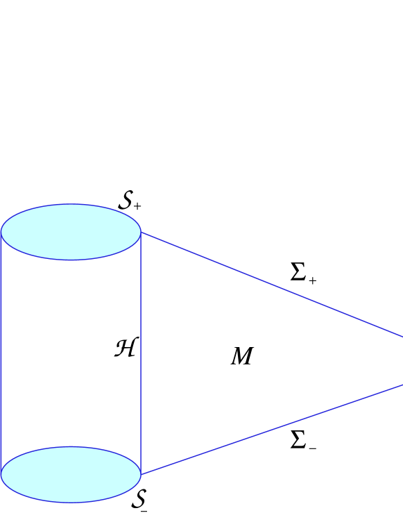
Figure 3.1: Domain of variation in ${\mathcal{M}}$ bounded by two Cauchy surfaces $\Sigma_{-}$ and $\Sigma_{+}$, spatial infinity $\tau_{\infty}$ and the WIH $({\mathcal{H}},[\bm{\ell}])$. ${\mathcal{S}}_{-}$ and ${\mathcal{S}}_{+}$ denote the cross-sections resulting from the intersections of the spatial slices $\Sigma_{-}$ and $\Sigma_{+}$ with the WIH.

In the variation of the action, the bulk term gives rise to a boundary term at infinity, but it is exactly cancelled by the variation of the boundary term at infinity in Eq. (C.1). The resulting variation can be expressed as

$$\delta S(\bm{e},\bm{A})=\int\mathrm{(Equations\ of\ Motion)}\cdot\delta(\bm{e},\bm{A})-\frac{1}{8\pi G}\int_{\mathcal{H}}\delta\bm{\omega}\wedge\bm{{}^{2}\epsilon}\ \ .$$ (C.3)

The problem is well-posed and Einstein equations are recovered as an extremal value of this action ( $\delta S(\bm{e},\bm{A})=0$), if the boundary integral at ${\mathcal{H}}$ vanishes. This is the crucial point we want to make in this example: the WIH condition ${}^{{\mathcal{H}}}\!\bm{\mathcal{L}}_{\bm{\bm{\ell}}}\,\bm{\omega}=0$, together with the NEH conditions and $\delta(\bm{e},\bm{A})=0$ on $\Sigma_{-}$ and $\Sigma_{+}$, suffices to guarantee the vanishing of this boundary term (see [10] for the details).

C.1.1 Phase space and canonical transformations

Once the variational problem is well-posed, we must determine the phase space $\Gamma$. We firstly introduce some general concepts and notation (see, e.g. Refs. [1, 8, 80]).

The phase space is constituted by a pair $(\Gamma,\bm{J})$, where $\Gamma$ is an (infinite-dimensional) manifold in which each point represents a solution to the equations of motion and $\bm{J}$ is a closed two-form on $\Gamma$ known as the symplectic form: $\bm{\mathrm{d}}^{\Gamma}\bm{J}=0$, with $\bm{\mathrm{d}}^{\Gamma}$ the exterior differential in $\Gamma$. We can associate with each function $F:\Gamma\rightarrow\mathbb{R}$, a Hamiltonian vector field $\delta_{F}$ in ${\mathcal{T}}(\Gamma)$ (the space of vector fields on $\Gamma$ in the notation introduced in Sec. 1.2) as follows

$$i_{\delta_{F}}\bm{J}=\bm{\mathrm{d}}^{\Gamma}F\ ,$$ (C.4)

where $i_{\delta_{F}}\bm{J}:=\bm{J}(\delta_{F},\cdot)$. Given two functions $F$ and $G$ with support on $\Gamma$, their Poisson bracket is defined as

$$\{F,G\}=\bm{J}(\delta_{F},\delta_{G})\ \ .$$ (C.5)

The pair $(\Gamma,\bm{J})$ is also known as a symplectic manifold (pre-symplectic if the kernel of $\bm{J}$ is non-trivial). Even though the phase spaces we are interested in are intrinsically infinite-dimensional, we shall skip all the subtleties related to infinite-dimensional symplectic spaces (see for instance [119]).

An infinitesimal transformation on the space $\Gamma$, generated by the vector field $\delta_{\bm{W}}$, is a canonical transformation (also called symplecto-morphism) if it preserves the symplectic form $\bm{J}$

$${}^{\Gamma}\!{\mathcal{L}}_{\delta_{\bm{W}}}\bm{J}=0\ .$$ (C.6)

Using the closed character of $\bm{J}$, this is locally equivalent to the existence of a Hamiltonian function $H_{\bm{W}}$, i.e.

$$\framebox{$\displaystyle\left.\begin{array}[]{l}\hbox{$\delta_{\bm{W}}$ preserves (locally)}\\ \hbox{the Poisson brackets}\end{array}\right\}\Longleftrightarrow\exists H_{\bm{W}}\,\hbox{ such that }\,i_{\delta_{W}}\bm{J}=\bm{\mathrm{d}}^{\Gamma}H_{\bm{W}}\ ,$}$$ (C.9)

Applying this expression to a generic vector field $\delta$ in ${\mathcal{T}}(\Gamma)$, yields

$$\bm{J}(\delta_{\bm{W}},\delta)=\delta H_{\bm{W}}\ ,$$ (C.10)

where the notation $\delta H_{W}:=\bm{\mathrm{d}}^{\Gamma}H_{\bm{W}}(\delta)$ is designed to mimic the intuitive physical notation. The evolution of a function $G$ along the flow of the vector field $\delta_{W}$ on $\Gamma$ (Hamilton equations), can be evaluated as

$$\delta_{\bm{W}}G=\{H_{\bm{W}},G\}\ .$$ (C.11)

In particular, due to the anti-symmetry of $\bm{J}$, $H_{\bm{W}}$ remains constant along the $\delta_{\bm{W}}$ trajectories. With these elements, the general strategy to associate physical parameters with the horizon will proceed via the following steps:

1. Construction of the appropriate phase space $\Gamma$ for our problem.

2. Extension of a given WIH-symmetry of $({\mathcal{H}},[\bm{\ell}])$ to an infinitesimal diffeomorphism $\bm{W}$ on each space-time ${\mathcal{M}}$ of $\Gamma$, giving rise to a family of vector fields $\{\bm{W}\}_{\Gamma}$. Definition of a canonical transformation $\delta_{\bm{W}}$ on $\Gamma$ out of the family $\{\bm{W}\}_{\Gamma}$.

3. Identification of the physical parameter with the associated conserved quantity $H_{\bm{W}}$.

We illustrate these steps by continuing Example C.1 (see again [15, 12]).

Example C.2

Phase space and canonical transformations.

(1) Phase space.

The phase space $\Gamma$ where we describe the dynamics defined by the action (C.1), can be parametrized by the pairs $(\bm{e}^{I},\bm{A}^{I}_{J})$ which satisfy Einstein equations and contain an inner boundary given by a “fixed” WIH $({\mathcal{H}},[\bm{\ell}])$. The so-called conserved current method [56] provides a standard manner to derive the relevant symplectic form from a given action. In our case this results in [12]

$$\bm{J}(\delta_{1},\delta_{2}) = -\frac{1}{16\pi G}\int_{\Sigma}\left(\delta_{1}\bm{\Sigma}^{IJ}\wedge\delta_{2}\bm{A}_{IJ}-\delta_{2}\bm{\Sigma}^{IJ}\wedge\delta_{1}\bm{A}_{IJ}\right)$$ (C.12)

$$+ \frac{1}{8\pi G}\int_{{\mathcal{S}}_{t}}\left(\delta_{1}\bm{{}^{2}\epsilon}\;\delta_{2}\psi-\delta_{2}\bm{{}^{2}\epsilon}\;\delta_{1}\psi\right)\ \ ,$$

where $\psi$ is a function on ${\mathcal{H}}$ such that ${}^{{\mathcal{H}}}\!\bm{\mathcal{L}}_{\bm{\bm{\ell}}}\,\psi:=\kappa_{(\bm{\ell})}$ and $\delta_{1},\delta_{2}$ are arbitrary vector fields on ${\mathcal{T}}(\Gamma)$.

(2) Canonical transformations induced by space-time transformations.

On each point of $\Gamma$, i.e. on each spacetime ${\mathcal{M}}$ represented by a pair $(\bm{e}^{I},\bm{A}^{I}_{J})$, we consider an infinitesimal spacetime diffeomorphism $\bm{W}(\bm{e},\bm{A})$ (we make explicit the dependence of this vector field on the particular spacetime) whose restriction to ${\mathcal{H}}$ is a WIH-symmetry. This family of spacetime vector fields $\{\bm{W}(\bm{e},\bm{A})\}$ permits us to define an infinitesimal transformation $\delta_{\bm{W}}$ on $\Gamma$, which is defined in a point-wise manner (on each point ${\mathcal{M}}$ of $\Gamma$) by its action on the coordinates $(\bm{e}^{I},\bm{A}^{I}_{J})$ of $\Gamma$

$$\left.\left(\delta_{\bm{W}}\bm{e}^{I}\right)\right|_{\mathcal{M}}:={\mathcal{L}}_{\bm{W}(\bm{e},\bm{A})}\bm{e}^{I}\ \ \ \ \ \ \ \left.\left(\delta_{\bm{W}}\bm{A}^{I}_{J}\right)\right|_{\mathcal{M}}:={\mathcal{L}}_{\bm{W}(\bm{e},\bm{A})}\bm{A}^{I}_{J}\ ,$$ (C.13)

where right-hand side terms are evaluated on each spacetime ${\mathcal{M}}$, associated respectively with the pair $(\bm{e}^{I},\bm{A}^{I}_{J})$. In sum, starting from a family of WIH-symmetries $\{\bm{W}(\bm{e},\bm{A})|_{{\mathcal{H}}}\}$ an infinitesimal transformation $\delta_{\bm{W}}$ has been induced in the phase space $\Gamma$ (see Fig. 3.2).

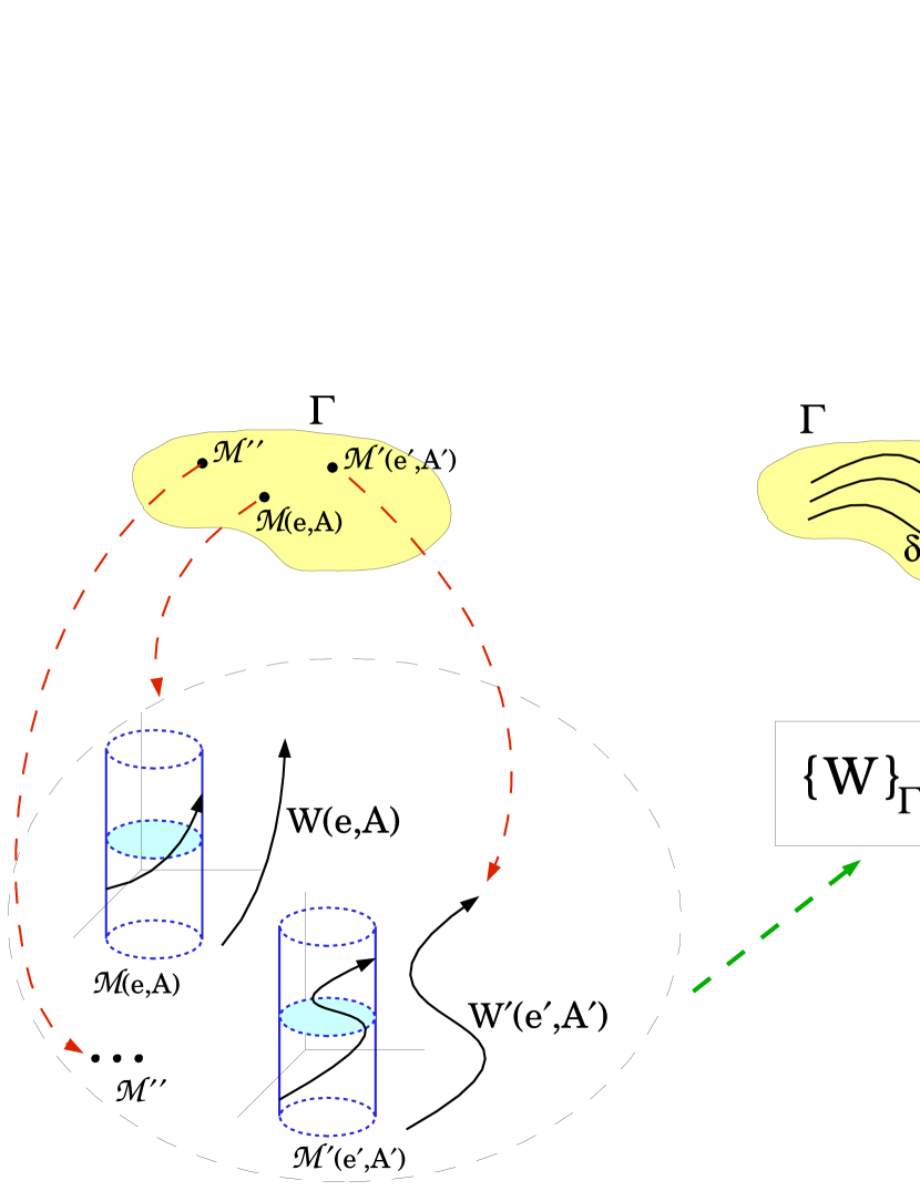
Figure 3.2: Illustration of the construction of a transformation $\delta_{\bm{W}}$ on $\Gamma$ from the family $\{\bm{W}\}_{\Gamma}$ on diffeomorphisms of spacetimes ${\mathcal{M}}$. On each point of $\Gamma$, a spacetime ${\mathcal{M}}(\bm{e},\bm{A})$, we consider a diffeomorphism $\bm{W}(\bm{e},\bm{A})$ whose restriction to ${\mathcal{H}}$ is a WIH-symmetry. The ensemble of these spacetime diffeomorphisms $\{\bm{W}(\bm{e},\bm{A})\}_{\Gamma}$ generates a transformation $\delta_{\bm{W}}$ on $\Gamma$ through Eq. (C.13).

The question now is to find out if such a transformation $\delta_{\bm{W}}$ is a canonical one. According to (C.9), one must contract the vector field $\delta_{\bm{W}}$ with the symplectic form (C.12) and check if the resulting 1-form on $\Gamma$ is (locally) exact. Following (C.10), this contraction is applied on an arbitrary vector field $\delta$

$$\bm{J}(\delta,\delta_{\bm{W}}) = \frac{-1}{8\pi G}\int_{{\mathcal{S}}_{t}}\delta\left[\langle\bm{q}^{*}\bm{W},\bm{\omega}\rangle\bm{{}^{2}\epsilon}\right]-\langle\delta\bm{q}^{*}\bm{W},\bm{\omega}\rangle\bm{{}^{2}\epsilon}+\kappa_{(\bm{W})}\delta\bm{{}^{2}\epsilon}$$ (C.14)

$$+ \frac{1}{16\pi G}\int_{\Sigma_{\infty}}\bm{A}^{IJ}\wedge\langle\bm{W},\Sigma_{IJ}\rangle+\langle\bm{W},\bm{A}^{IJ}\rangle\delta\Sigma_{IJ}\ ,$$

where $\kappa_{(\bm{W})}=\langle\bm{W}-\bm{q}^{*}\bm{W},\bm{\omega}\rangle$.

(3) Conserved quantities and horizon physical parameters.

The term at infinity is related to the standard ADM quantities (whenever $\bm{W}$ is a symmetry of the asymptotic metric at infinity). Consequently, it is associated with the exact variation of a function on $\Gamma$, the corresponding ADM parameter. Likewise, in order to associate a conserved quantity with the horizon ${\mathcal{H}}$ itself, the integral on ${\mathcal{S}}_{t}$ must be written as the exact variation of a function on $\Gamma$. We study this problem for the specific and physically relevant cases of the angular momentum and the energy.

C.2 Applications of examples (C.1) and (C.2)

We offer some more details on the discussion developed in Secs. 8.6.1 and 8.6.2.

C.2.1 Angular momentum

We restrict $\Gamma$ to its subspace $\Gamma_{\bm{\phi}}$ of spacetimes containing a class II WIH. On the inner boundary ${\mathcal{H}}$ of each spacetime ${\mathcal{M}}$, the same rigid azimuthal WIH-symmetry $\bm{\phi}$ is fixed (in fact $\bm{\phi}$ is an isometry of the cross-section ${\mathcal{S}}_{t}$). More specifically, we consider on every spacetime in $\Gamma_{\bm{\phi}}$ a vector field $\bm{\phi}$ which is a $SO(2)$ axial isometry of the induced metric $\bm{q}$ on ${\mathcal{H}}$ with $2\pi$ affine length.

This WIH-symmetry on ${\mathcal{H}}$ is then extended to a vector field $\bm{\varphi}$ on each spacetime ${\mathcal{M}}$. Since we are interested in studying the angular momentum related to the horizon itself, this extension $\bm{\varphi}$ is enforced to vanish outside some compact neighbourhood of the horizon. Evaluating expression (C.14) in this case, results in [12]

$$\bm{J}(\delta,\delta_{\bm{\varphi}})=\delta\left(\frac{-1}{8\pi G}\int_{{\mathcal{S}}_{t}}\bm{\phi}\cdot\bm{\omega}\ \bm{{}^{2}\epsilon}\right)\ .$$ (C.15)

The transformation $\delta_{\bm{\varphi}}$ induces directly a locally canonical transformation on $\Gamma_{\bm{\phi}}$. Making $J_{\mathcal{H}}:=H_{\bm{\varphi}}$, the conserved quantity $J_{{\mathcal{H}}}$ is identified as the angular momentum associated with the horizon and Eq. (8.6.1) follows. We also point out that this expression is conserved under the canonical transformation $\delta_{\bm{\varphi}}$ in $\Gamma$, even if $\bm{\phi}$ is not a WIH-symmetry. However, as mentioned in Sec. 8.6.1, in the absence of a symmetry the physical status of this expression is unclear.

C.2.2 Mass

As discussed in Sec. 8.6.2, the definition of the mass is related to the choice of an evolution vector $\bm{t}$ on each spacetime ${\mathcal{M}}$, which plays now the role of the vector $\bm{W}$ in Example C.2. We fix expression (8.35) as the inner boundary condition for $\bm{t}$. Regarding the outer boundary condition at infinity, we make $\bm{t}$ to approach an observer $\bm{t}_{\infty}$ inertial with respect to the flat metric.

The first law of black hole mechanics (8.36) follows from imposing $\delta_{\bm{t}}$ to be a locally canonical transformation on $\Gamma_{\bm{\phi}}$. Expression (C.14) in this case simplifies to

$$\bm{J}(\delta,\delta_{\bm{t}})=\delta E^{t}_{\mathrm{ADM}}-\left(\frac{\kappa_{(t)}}{8\pi G}\delta a_{\mathcal{H}}+\Omega_{(t)}\delta J_{\mathcal{H}}\right)\ \ ,$$ (C.16)

where $E^{t}_{\mathrm{ADM}}$ corresponds to the ADM energy and $a_{\mathcal{H}}=\int_{{\mathcal{S}}}\bm{{}^{2}\epsilon}$ is the area of ${\mathcal{S}}_{t}$. On each spacetime ${\mathcal{M}}$ in $\Gamma$, $\kappa_{(\bm{t})}$ and $\Omega_{(\bm{t})}$ are constant. However, the actual values of these constants change from one spacetime to another: $\kappa_{(\bm{t})}$ and $\Omega_{(\bm{t})}$ are functions on $\Gamma$. As a necessary condition for $\bm{J}(\cdot,\delta_{t})$ to be an exact variation on $\Gamma$ so as to make $\delta_{\bm{t}}$ a canonical transformation via Eq. (C.10), the form $\bm{J}(\cdot,\delta_{t})$ must be closed. Consequently, functions $\kappa_{(\bm{t})}$ and $\Omega_{(\bm{t})}$ depend on $\Gamma$ only through an explicit dependence on $a_{\mathcal{H}}$ and $J_{\mathcal{H}}$, satisfying

$$\frac{\partial\kappa_{(t)}(a_{\mathcal{H}},J_{\mathcal{H}})}{\partial J_{\mathcal{H}}}=8\pi G\frac{\partial\Omega_{(t)}(a_{\mathcal{H}},J_{\mathcal{H}})}{\partial a_{\mathcal{H}}}\ .$$ (C.17)

If $\delta_{\bm{t}}$ is indeed a canonical infinitesimal transformation, we can write the second term in the right-hand side of Eq.(C.16) as an exact variation $\delta E^{t}_{\mathcal{H}}$, and Eq. (8.36) follows. As mentioned in Sec. 8.6.2, this does not fix the functional forms of $\kappa_{(\bm{t})}(a_{\mathcal{H}},J_{\mathcal{H}})$, $\Omega_{(\bm{t})}(a_{\mathcal{H}},J_{\mathcal{H}})$ and $E^{t}_{\mathcal{H}}$. Finally, these dependences of the physical parameters in $a_{\mathcal{H}}$ and $J_{\mathcal{H}}$, which are the same for all spacetimes in $\Gamma_{\bm{\phi}}$, are fixed by making them to coincide with those of the Kerr family (a subspace of $\Gamma_{\bm{\phi}}$), as explained in Sec. 8.6.2.

Appendix D Illustration with the event horizon of a Kerr black hole

In Examples 2.5, 3.1, 4.6, 5.7 and 6.5, we have considered for simplicity a non-rotating static black hole (Schwarzschild spacetime). It is of course interesting to investigate rotating stationary black holes (Kerr spacetime) as well. In particular, the Háj́iček  1-form which has been found to vanish for a Schwarzschild horizon [Eq. (5.105)] is no longer zero for a Kerr horizon. We discuss here the event horizon ${\mathcal{H}}$ of a Kerr black hole from the 3+1 decomposition introduced in Sec. 10, by considering a foliation $(\Sigma_{t})$ based on Kerr coordinates.

D.1 Kerr coordinates

In standard textbooks, the Kerr solution is presented in Boyer-Lindquist coordinates $(t_{\rm BL},r,\theta,\varphi_{\rm BL})$. However, being a generalization of Schwarzschild coordinates to the rotating case, these coordinates are singular on the event horizon ${\mathcal{H}}$, as discussed in Example 2.5. We consider instead Kerr coordinates, which are regular on ${\mathcal{H}}$. These are the coordinates in which Kerr originally exhibited his solution [104]; they are a generalization of Eddington-Finkelstein coordinates to the rotating case. Denoting them by $(V,r,\theta,\varphi)$, they are such that the curves $V={\rm const}$, $\theta={\rm const}$ and $\varphi={\rm const}$ are ingoing null geodesics (they form a so-called principal null congruence), as in the Eddington-Finkelstein case. As in the Schwarzschild case, we will use the coordinate

$$t:=V-r$$ (D.1)

instead of $V$ [cf. Eq. (2.33)]. The coordinates $(t,r,\theta,\varphi)$ are then simply a spheroidal version of the well-known Kerr-Schild coordinates $(t,x,y,z)$: $t$ is the same coordinate and $(x,y,z)$ are related to $(r,\theta,\varphi)$ by

$$x=(r\cos\varphi-a\sin\varphi)\sin\theta,\quad y=(r\sin\varphi+a\cos\varphi)\sin\theta,\quad$$

$$z=r\cos\theta,$$ (D.2)

where $a$ is the angular momentum parameter of the Kerr solution, i.e. the quotient of the total angular momentum $J$ by the total mass $m$, $a:=J/m$. The relation with the Boyer Lindquist coordinates $(t_{\rm BL},r,\theta,\varphi_{\rm BL})$ is as follows:

$$dt=dt_{\rm BL}+\frac{dr}{\frac{r^{2}+a^{2}}{2mr}-1}\quad\mbox{and}\quad d\varphi=d\varphi_{\rm BL}+\frac{a\,dr}{r^{2}-2mr+a^{2}}\ \ .$$ (D.3)

The metric components with respect to the “3+1” Kerr coordinates $(t,r,\theta,\varphi)$ are given by

$$g_{\mu\nu}dx^{\mu}dx^{\nu} = -\left(1-\frac{2mr}{\rho^{2}}\right)dt^{2}+\frac{4mr}{\rho^{2}}\,dt\,dr-\frac{4amr}{\rho^{2}}\sin^{2}\theta\,dt\,d\varphi$$ (D.4)

$$+\left(1+\frac{2mr}{\rho^{2}}\right)dr^{2}-2a\sin^{2}\theta\left(1+\frac{2mr}{\rho^{2}}\right)dr\,d\varphi$$

$$+\rho^{2}d\theta^{2}+\left(r^{2}+a^{2}+\frac{2a^{2}mr\sin^{2}\theta}{\rho^{2}}\right)\sin^{2}\theta d\varphi^{2},$$

with

$$\rho^{2}:=r^{2}+a^{2}\cos^{2}\theta.$$ (D.5)

The event horizon ${\mathcal{H}}$ is located at

$$r=r_{{\mathcal{H}}}:=m+\sqrt{m^{2}-a^{2}}.$$ (D.6)

Since $r_{{\mathcal{H}}}$ does not depend upon $\theta$ nor $\varphi$, the Kerr coordinates are adapted to ${\mathcal{H}}$, according to the terminology introduced in Sec. 4.8. Note that the metric components given by Eq. (D.4) are all regular at $r=r_{{\mathcal{H}}}$. On the contrary, most of them are singular at $\rho=0$, which, via Eq. (D.5), corresponds to $r=0$ and $\theta=\pi/2$, and, via Eq. (D.2), to the ring $x^{2}+y^{2}=a^{2}$ in the plane $z=0$. This is the ring singularity of Kerr spacetime. Note also that in the limit $a\rightarrow 0$, then $\rho\rightarrow r$ and the line element (D.4) reduces to the line element (2.34) in Eddington-Finkelstein coordinates. The metric (D.4) is clearly stationary and axisymmetric and the two vectors

$$\bm{\xi}_{0}:=\left(\frac{\partial}{\partial t}\right)_{r,\theta,\varphi}\qquad\mbox{and}\qquad\bm{\xi}_{1}:=\left(\frac{\partial}{\partial\varphi}\right)_{t,r,\theta}$$ (D.7)

are two Killing vectors, $\bm{\xi}_{0}$ being associated with the stationarity and $\bm{\xi}_{1}$ with the axial symmetry of the Kerr spacetime.

Remark D.1

The two Killing vectors $\bm{\xi}_{0}$ and $\bm{\xi}_{1}$ are identical to the “standard” two Killing vectors which are formed from the Boyer-Lindquist coordinates:

$$\bm{\xi}_{0}=\left(\frac{\partial}{\partial t_{\rm BL}}\right)_{r,\theta,\varphi_{\rm BL}}\qquad\mbox{and}\qquad\bm{\xi}_{1}=\left(\frac{\partial}{\partial\varphi_{\rm BL}}\right)_{t_{\rm BL},r,\theta}.$$ (D.8)

This properties follows easily from the transformation law (D.3) between the two sets of coordinates. Consequently, the metric coefficients $g_{tt}=\bm{\xi}_{0}\cdot\bm{\xi}_{0}$, $g_{t\varphi}=\bm{\xi}_{0}\cdot\bm{\xi}_{1}$ and $g_{\varphi\varphi}=\bm{\xi}_{1}\cdot\bm{\xi}_{1}$, which can be read on Eq. (D.4) are the same than those for Boyer-Lindquist coordinates, as it can be checked by comparing with e.g. Eq. (33.2) in MTW [123].

D.2 3+1 quantities

Let us consider the foliation of Kerr spacetime by the hypersurfaces $\Sigma_{t}$ of constant Kerr time $t$. From the line element (D.4), we read the corresponding lapse function

$$N=\frac{\rho}{\sqrt{\rho^{2}+2mr}},$$ (D.9)

the shift vector

$$\beta^{i}=\left(\frac{2mr}{\rho^{2}+2mr},0,0\right)\quad\mbox{and}\quad\beta_{i}=\left(\frac{2mr}{\rho^{2}},0,-\frac{2amr}{\rho^{2}}\sin^{2}\theta\right)$$ (D.10)

and the 3-metric

$$\gamma_{ij}=\left(\begin{array}[]{ccc}1+\frac{2mr}{\rho^{2}}&0&-a\left(1+\frac{2mr}{\rho^{2}}\right)\sin^{2}\theta\\ 0&\rho^{2}&0\\ -a\left(1+\frac{2mr}{\rho^{2}}\right)\sin^{2}\theta&0&\frac{A}{\rho^{2}}\sin^{2}\theta\end{array}\right),$$ (D.11)

$$\gamma^{ij}=\left(\begin{array}[]{ccc}\frac{A}{\rho^{2}(\rho^{2}+2mr)}&0&\frac{a}{\rho^{2}}\\ 0&\rho^{-2}&0\\ \frac{a}{\rho^{2}}&0&\frac{1}{\rho^{2}\sin^{2}\theta}\end{array}\right),$$ (D.12)

with

$$A := (r^{2}+a^{2})^{2}-(r^{2}-2mr+a^{2})a^{2}\sin^{2}\theta$$ (D.13)

$$= \rho^{2}(r^{2}+a^{2})+2a^{2}mr\sin^{2}\theta.$$

The unit timelike normal to $\Sigma_{t}$ is deduced from the values of the lapse function and the shift vector via Eq. (3.24), which results in

$$n^{\alpha} = \left(\frac{1}{\rho}\sqrt{\rho^{2}+2mr},-\frac{2mr}{\rho\sqrt{\rho^{2}+2mr}},0,0\right)$$ (D.14)

$$n_{\alpha} = \left(-\frac{\rho}{\sqrt{\rho^{2}+2mr}},0,0,0\right).$$ (D.15)

Finally the extrinsic curvature tensor of $\Sigma_{t}$ is obtained from Eq. (3.42) with $\partial\gamma_{ij}/\partial t=0$:

$$K_{ij} = \left(\begin{array}[]{ccc}\frac{2m(a^{2}\cos^{2}\theta-r^{2})(\rho^{2}+mr)}{\rho^{5}\sqrt{\rho^{2}+2mr}}&\frac{2a^{2}mr\sin\theta\cos\theta}{\rho^{3}\sqrt{\rho^{2}+2mr}}&\frac{am(r^{2}-a^{2}\cos^{2}\theta)\sin^{2}\theta\sqrt{\rho^{2}+2mr}}{\rho^{5}}\\[14.22636pt] {\rm sym.}&\frac{2mr^{2}}{\rho\sqrt{\rho^{2}+2mr}}&-\frac{2a^{3}mr\sin^{3}\theta\cos\theta}{\rho^{3}\sqrt{\rho^{2}+2mr}}\\[14.22636pt] {\rm sym.}&{\rm sym.}&\displaystyle{\frac{2mr\sin^{2}\theta}{\rho\sqrt{\rho^{2}+2mr}}\times\atop\left[r+\frac{a^{2}m(a^{2}\cos^{2}\theta-r^{2})\sin^{2}\theta}{\rho^{4}}\right]}\end{array}\right).$$ (D.19)

As a check of this formula, we may compare it with Eqs. (A2.33)-(A2.38) of Ref. [161].

D.3 Unit normal to ${\mathcal{S}}_{t}$ and null normal to ${\mathcal{H}}$

The 2-surface ${\mathcal{S}}_{t}\subset\Sigma_{t}$ is defined by $r={\rm const}=r_{{\mathcal{H}}}$. Its outward unit normal $\bm{s}$ lying in $\Sigma_{t}$ is obtained from $s_{i}=(\alpha,0,0)$, with $\alpha$ such that $\gamma^{ij}s_{i}s_{j}=1$. We get

$$s_{i} = \left(\rho\sqrt{\frac{\rho^{2}+2mr}{A}},\ 0,\ 0\right),$$ (D.21)

$$s^{i} = \left(\frac{1}{\rho}\sqrt{\frac{A}{\rho^{2}+2mr}},\ 0,\ \frac{a}{\rho}\sqrt{\frac{\rho^{2}+2mr}{A}}\right).$$ (D.22)

As a check, we verify that $\bm{n}$ and $\bm{s}$ given by Eqs. (D.14) and (D.22) coincide with the first two vectors of the orthonormal basis $(\vec{\bm{E}}_{\alpha})$ introduced by King et al. [105] [cf. their Eq. (2.4), noticing that their coordinate vectors are $\left(\partial/\partial V\right)_{r,\theta,\varphi}=\left(\partial/\partial t\right)_{r,\theta,\varphi}$ and $\left(\partial/\partial r\right)_{V,\theta,\varphi}=\left(\partial/\partial r\right)_{t,\theta,\varphi}-\left(\partial/\partial t\right)_{r,\theta,\varphi}$].

We then get the null normal to ${\mathcal{H}}$ associated with the Kerr slicing, $\bm{\ell}$, by inserting expressions (D.9), (D.14) and (D.22) into $\bm{\ell}=N(\bm{n}+\bm{s})$ [Eq. (4.13)]:

$$\ell^{\alpha}=\left(1,\ \frac{\sqrt{A}-2mr}{\rho^{2}+2mr},\ 0,\ \frac{a}{\sqrt{A}}\right).$$ (D.23)

The value on the horizon is obtained by noticing that $A\stackrel{{\scriptstyle{\mathcal{H}}}}{{=}}(2mr_{{\mathcal{H}}})^{2}$; we get $\ell^{\alpha}\stackrel{{\scriptstyle{\mathcal{H}}}}{{=}}(1,0,0,a/(2mr_{{\mathcal{H}}}))$, i.e., from Eq. (D.7),

$$\framebox{$\displaystyle\bm{\ell}\stackrel{{\scriptstyle{\mathcal{H}}}}{{=}}\bm{\xi}_{0}+\Omega_{{\mathcal{H}}}\,\bm{\xi}_{1}$},$$ (D.24)

with

$$\framebox{$\displaystyle\Omega_{{\mathcal{H}}}:=\frac{a}{2mr_{{\mathcal{H}}}}=\frac{a}{2m(m+\sqrt{m^{2}-a^{2}})}$}.$$ (D.25)

Eq. (D.24) shows that on the horizon, the null normal $\bm{\ell}$ is a linear combination of the two Killing vectors $\bm{\xi}_{0}$ and $\bm{\xi}_{1}$ with constant coefficients (compare with the inner boundary (8.35) for the evolution vector $\bm{t}$ in Sec. 8.6.2). It is therefore a Killing vector itself. This implies

$$\bm{\mathcal{L}}_{\bm{\bm{\ell}}}\,\bm{A}\stackrel{{\scriptstyle{\mathcal{H}}}}{{=}}0,$$ (D.26)

for any tensor field $\bm{A}$ which respects the stationarity and axisymmetry of the Kerr spacetime. Another phrasing of this is saying that ${\mathcal{H}}$ is a Killing horizon [36]. Comparing Eq. (D.24) with Eq. (4.80) (taking into account that $\bm{t}=\bm{\xi}_{0}$), we get the surface velocity of ${\mathcal{H}}$ with respect to Kerr coordinates:

$$\framebox{$\displaystyle\bm{V}=\Omega_{{\mathcal{H}}}\,\bm{\xi}_{1}=\Omega_{{\mathcal{H}}}\,\left(\frac{\partial}{\partial\varphi}\right)_{t,r,\theta}$}.$$ (D.27)

Hence the quantity $\Omega_{{\mathcal{H}}}$ can be viewed as the angular velocity of ${\mathcal{H}}$ with respect to the coordinates $(t,r,\theta,\varphi)$. The fact that $\Omega_{{\mathcal{H}}}$ is a constant over ${\mathcal{H}}$ reflects the rigidity theorem of stationary black holes (see e.g. Theorem 4.2 of Ref. [37]; more generally, in the WIH setting of Sec. 8, the constancy of $\Omega_{{\mathcal{H}}}$ guarantees $\bm{t}$ to be a WIH-symmetry on ${\mathcal{H}}$).

D.4 3+1 evaluation of the surface gravity $\kappa$

We will need the orthogonal projector $\vec{\bm{q}}$ on ${\mathcal{S}}_{t}$. Its components with respect to the coordinates $(r,\theta,\varphi)$ are given by the formula $q^{i}_{\ \,j}=\delta^{i}_{\ \,j}-s^{i}s_{j}$; from Eqs. (D.21)-(D.22), we get ($i$ = row index, $j$ = column index)

$$q^{i}_{\ \,j}=\left(\begin{array}[]{ccc}0&0&0\\ 0&1&0\\ \displaystyle-\frac{a}{A}\left(\rho^{2}+2mr\right)&0&1\end{array}\right).$$ (D.28)

We will also need the 1-form $\bm{K}(\bm{s},.)$. From Eqs. (LABEL:e:KE:Kij) and (D.22), we get

$$K_{rj}s^{j} = \frac{m(r^{2}-a^{2}\cos^{2}\theta)}{\rho^{4}(\rho^{2}+2mr)\sqrt{A}}\left[\rho^{2}a^{2}\sin^{2}\theta-2(\rho^{2}+mr)(r^{2}+a^{2})\right]$$

$$K_{\theta j}s^{j} = \frac{2a^{2}mr\sin\theta\cos\theta}{(\rho^{2}+2mr)\sqrt{A}}$$

$$K_{\varphi j}s^{j} = \frac{am\sin^{2}\theta}{\rho^{4}\sqrt{A}}\left[r^{2}(3r^{2}+a^{2}\cos^{2}\theta)+a^{2}(r^{2}-a^{2}\cos^{2}\theta)\right].$$ (D.29)

Let us start by evaluating the non-affinity parameter $\kappa$ from the 3+1 expression (10.10). The first part of this relation is computed from Eqs. (D.23) and (D.9):

$$\ell^{\mu}\nabla_{\mu}\ln N=\frac{m}{\rho^{2}}\frac{r^{2}-a^{2}\cos^{2}\theta}{(\rho^{2}+2mr)^{2}}(\sqrt{A}-2mr).$$ (D.30)

Since $A\stackrel{{\scriptstyle{\mathcal{H}}}}{{=}}(2mr_{{\mathcal{H}}})^{2}$, this implies

$$\ell^{\mu}\nabla_{\mu}\ln N\stackrel{{\scriptstyle{\mathcal{H}}}}{{=}}0,$$ (D.31)

in agreement with Eq. (D.26). The second term in the right-hand side of Eq. (10.10) is computed from Eqs. (D.22) and (D.9)

$$s^{i}D_{i}N=\frac{m}{\rho^{2}}\frac{(r^{2}-a^{2}\cos^{2}\theta)\sqrt{A}}{(\rho^{2}+2mr)^{2}},$$ (D.32)

resulting in the following value on the horizon

$$s^{i}D_{i}N\stackrel{{\scriptstyle{\mathcal{H}}}}{{=}}\frac{2m^{2}r_{{\mathcal{H}}}(r_{{\mathcal{H}}}^{2}-a^{2}\cos^{2}\theta)}{\rho_{{\mathcal{H}}}^{2}(\rho_{{\mathcal{H}}}^{2}+2mr_{{\mathcal{H}}})^{2}},$$ (D.33)

with $\rho_{{\mathcal{H}}}^{2}:=r_{{\mathcal{H}}}^{2}+a^{2}\cos^{2}\theta=2mr_{{\mathcal{H}}}-a^{2}\sin^{2}\theta$. Finally from Eqs. (D.9), (D.29) and (D.22), we evaluate the last term which enters in formula (10.10), namely $NK_{ij}s^{i}s^{j}$. The obtained expression is rather complicated; however combining its value on the horizon with the results (D.31) and (D.33) yields a very simple expression for the non-affinity parameter:

$$\framebox{$\displaystyle\kappa=\frac{r_{{\mathcal{H}}}-m}{2mr_{{\mathcal{H}}}}=\frac{\sqrt{m^{2}-a^{2}}}{2m(m+\sqrt{m^{2}-a^{2}})}$}.$$ (D.34)

Note that $\kappa$ does not depend on $\theta$, in agreement with the fact that ${\mathcal{H}}$, endowed with the null normal $\bm{\ell}$ given by Eq. (D.24), is an isolated horizon [zeroth law of black hole mechanics, cf. Eq. (8.5)]. Actually we recover for $\kappa$ the classical value of the surface gravity of a Kerr black hole (see e.g. Eq. (12.5.4) of Wald [167]).

D.5 3+1 evaluation of the Háj́iček 1-form $\bm{\Omega}$

Let us now compute the Háj́iček 1-form from the 3+1 formula (10.14). From Eqs. (D.9), (D.29) and (D.28), we get

$$\Omega_{\theta} = -\frac{2a^{2}mr\sin\theta\cos\theta}{\rho^{2}+2mr}\left(\frac{1}{\sqrt{A}}+\frac{1}{\rho^{2}}\right)$$ (D.35)

$$\Omega_{\varphi} = -\frac{am\sin^{2}\theta}{\rho^{4}\sqrt{A}}\left[r^{2}(3r^{2}+a^{2}\cos^{2}\theta)+a^{2}(r^{2}-a^{2}\cos^{2}\theta)\right],$$ (D.36)

from which we deduce the following values on the horizon:

$$\Omega_{\theta} \stackrel{{\scriptstyle{\mathcal{H}}}}{{=}} -\frac{a^{2}\sin\theta\cos\theta}{2mr_{{\mathcal{H}}}-a^{2}\sin^{2}\theta}$$ (D.37)

$$\Omega_{\varphi} \stackrel{{\scriptstyle{\mathcal{H}}}}{{=}} \frac{a}{r_{{\mathcal{H}}}}\sin^{2}\theta\frac{(2m^{2}-3mr_{{\mathcal{H}}}+r_{{\mathcal{H}}}^{2})\cos^{2}\theta-r_{{\mathcal{H}}}(r_{{\mathcal{H}}}+m)}{(r_{{\mathcal{H}}}+(2m-r_{{\mathcal{H}}})\cos^{2}\theta)^{2}}.$$ (D.38)

As a check, let us recover the total angular momentum $J_{{\mathcal{H}}}=am$ from the integral (8.6.1) which involves $\bm{\Omega}$. The symmetry generator $\bm{\phi}$ which appears in the integral is of course in the present case the Killing vector $\bm{\xi}_{1}=\left(\partial/\partial{\varphi}\right)_{t,r,\theta}$, so that formula (8.6.1) results in ($G=1$)

$$J_{{\mathcal{H}}}=-\frac{1}{8\pi}\int_{{\mathcal{S}}_{t}}\Omega_{\varphi}\,\bm{{}^{2}\!\epsilon}.$$ (D.39)

Let us express the integral in terms of the coordinates $(\theta,\varphi)$ which span ${\mathcal{S}}_{t}$:

$$J_{{\mathcal{H}}}=-\frac{1}{8\pi}\int_{0}^{\pi}\int_{0}^{2\pi}\Omega_{\varphi}\,\sqrt{q}\,d\theta\,d\varphi,$$ (D.40)

where $q=\det q_{ab}$, with the 2-metric components $q_{ab}$ read from Eq. (D.11):

$$q_{ab}=\left(\begin{array}[]{cc}\rho^{2}&0\\ 0&\displaystyle\frac{A}{\rho^{2}}\sin^{2}\theta\end{array}\right).$$ (D.41)

Hence $\sqrt{q}=\sqrt{A}\sin\theta$, so that $\sqrt{q}\stackrel{{\scriptstyle{\mathcal{H}}}}{{=}}2mr_{{\mathcal{H}}}\sin\theta$ and the integral (D.40) becomes

$$J_{{\mathcal{H}}}=-\frac{2mr_{{\mathcal{H}}}}{8\pi}\int_{0}^{\pi}\int_{0}^{2\pi}\Omega_{\varphi}\,\sin\theta\,d\theta\,d\varphi.$$ (D.42)

Substituting Eq. (D.38) for $\Omega_{\varphi}$, we get

$$J_{{\mathcal{H}}}=-\frac{am}{4}\int_{0}^{\pi}\frac{(2\lambda-1)(\lambda-1)\cos^{2}\theta-\lambda(2\lambda+1)}{(\lambda+(1-\lambda)\cos^{2}\theta)^{2}}\,\sin^{3}\theta\,d\theta,$$ (D.43)

where we have set $\lambda:=r_{{\mathcal{H}}}/(2m)$. It turns out that the above integral is independent of $\lambda$ and is simply equal to $-4$, hence

$$\framebox{$\displaystyle J_{{\mathcal{H}}}=am$},$$ (D.44)

as it should be for a Kerr black hole.

D.6 3+1 evaluation of $\bm{\Theta}$ and $\bm{\Xi}$

In order to apply the formulæ derived in Sec. 10.3.2, let us first compute the second fundamental form $\bm{H}$ of the 2-surface ${\mathcal{S}}_{t}$ (as a hypersurface of $\Sigma_{t}$). From the relation $H_{ij}=D_{k}s_{l}\,q^{k}_{\ \,i}q^{l}_{\ \,j}$ [Eq. (10.30)] and expressions (D.21) and (D.28), we get the following values on the horizon:

$$H_{\theta\theta} \stackrel{{\scriptstyle{\mathcal{H}}}}{{=}} \frac{2mr_{{\mathcal{H}}}^{2}}{\sqrt{(2mr_{{\mathcal{H}}}-a^{2}\sin^{2}\theta)(4mr_{{\mathcal{H}}}-a^{2}\sin^{2}\theta})},$$ (D.45)

$$H_{\theta\varphi} \stackrel{{\scriptstyle{\mathcal{H}}}}{{=}} -\frac{2a^{3}mr_{{\mathcal{H}}}\sin^{3}\theta\cos\theta}{(2mr_{{\mathcal{H}}}-a^{2}\sin^{2}\theta)^{3/2}(4mr_{{\mathcal{H}}}-a^{2}\sin^{2}\theta)^{1/2}},$$ (D.46)

$$H_{\varphi\varphi} \stackrel{{\scriptstyle{\mathcal{H}}}}{{=}} \frac{mr_{{\mathcal{H}}}^{3}\sin^{2}\theta}{4(2mr_{{\mathcal{H}}}-a^{2}\sin^{2}\theta)^{5/2}(4mr_{{\mathcal{H}}}-a^{2}\sin^{2}\theta)^{1/2}}\times$$

$$\left[4m^{3}+9mr_{{\mathcal{H}}}^{2}+3r_{{\mathcal{H}}}^{3}-4a^{2}(r_{{\mathcal{H}}}+3m)\cos 2\theta+a^{4}\frac{m-r_{{\mathcal{H}}}}{r_{{\mathcal{H}}}^{2}}\cos 4\theta\right].$$

We are then in position to evaluate ${\mathcal{H}}$’s second fundamental form $\bm{\Theta}$ via Eq. (10.43): $\bm{\Theta}=N(\bm{H}-\vec{\bm{q}}^{*}\bm{K})$. Using the value of $\bm{K}$ and $\vec{\bm{q}}$ given by Eqs. (LABEL:e:KE:Kij) and (D.28), we get

$$\framebox{$\displaystyle\bm{\Theta}\stackrel{{\scriptstyle{\mathcal{H}}}}{{=}}0$}.$$ (D.48)

Hence we recover the fact that the event horizon of a Kerr black hole is a non-expanding horizon.

Regarding the transversal deformation rate $\bm{\Xi}$, we use the formula $\bm{\Xi}=-1/(2N)\,(\bm{H}-\vec{\bm{q}}^{*}\bm{K})$ [Eq. (10.44)]. Using expressions (D.45)-(LABEL:e:KE:Hpp), (LABEL:e:KE:Kij), (D.28) and (D.9), we get

$$\Xi_{\theta\theta} \stackrel{{\scriptstyle{\mathcal{H}}}}{{=}} -\frac{2mr_{{\mathcal{H}}}^{2}}{2mr_{{\mathcal{H}}}-a^{2}\sin^{2}\theta},$$ (D.49)

$$\Xi_{\theta\varphi} \stackrel{{\scriptstyle{\mathcal{H}}}}{{=}} \frac{2a^{3}mr\sin^{3}\theta\cos\theta}{(2mr_{{\mathcal{H}}}-a^{2}\sin^{2}\theta)^{2}},$$ (D.50)

$$\Xi_{\varphi\varphi} \stackrel{{\scriptstyle{\mathcal{H}}}}{{=}} -\frac{2mr_{{\mathcal{H}}}\sin^{2}\theta}{2mr_{{\mathcal{H}}}-a^{2}\sin^{2}\theta}\left[r_{{\mathcal{H}}}+\frac{a^{2}m(a^{2}\cos^{2}\theta-r_{{\mathcal{H}}}^{2})\sin^{2}\theta}{(2mr_{{\mathcal{H}}}-a^{2}\sin^{2}\theta)^{2}}\right].$$ (D.51)

Contracting with $q^{ab}$ [obtained as the inverse of the matrix (D.41)], we get the transversal expansion scalar

$$\theta_{(\bm{k})}\stackrel{{\scriptstyle{\mathcal{H}}}}{{=}}-\frac{2m+3r_{{\mathcal{H}}}-\frac{a^{2}}{m}\left[1+\left(\frac{m}{r_{{\mathcal{H}}}}-1\right)\cos^{2}\theta\right]}{2(2mr_{{\mathcal{H}}}-a^{2}\sin^{2}\theta)}.$$ (D.52)

As a check, one can easily verify that in the non-rotating limit ($a=0$, $r_{{\mathcal{H}}}=2m$), the values of $\bm{\Omega}$, $\bm{\Xi}$ and $\theta_{(\bm{k})}$ derived above reduce to that obtained in Example 5.7 for the Eddington-Finkelstein slicing of the Schwarzschild horizon [cf. Eqs. (5.104) and (5.105)].

Appendix E Symbol summary

The various metrics and associated connections (intrinsic geometries) used in this article are collected in Table 5.1, whereas the symbols used to describe the extrinsic geometries of the various submanifolds are collected in Table 5.2.

Manifold	Metric	Signature	Compatible	Ricci
			connection	tensor
${\mathcal{M}}$	$\bm{g}$	$(-,+,+,+)$	$\bm{\nabla}$	$\bm{R}$
${\mathcal{H}}$	$\bm{q}$	$(0,+,+)$	$\times$	$\times$
$\Sigma_{t}$	$\bm{\gamma}$	$(+,+,+)$	$\bm{D}$	${}^{3}\!\bm{R}$
$\Sigma_{t}$	$\bm{\tilde{\gamma}}$	$(+,+,+)$	$\bm{\tilde{D}}$	${}^{3}\!\bm{\tilde{R}}$
${\mathcal{S}}_{t}$	$\bm{q}$	$(+,+)$	$\bm{{}^{2}\!D}$	${}^{2}\!\bm{R}$
${\mathcal{S}}_{t}$	$\bm{\tilde{q}}$	$(+,+)$	$\bm{{}^{2}\!\tilde{D}}$	${}^{2}\!\bm{\tilde{R}}$
${\mathcal{H}}$ NEH	$\bm{q}$	$(0,+,+)$	$\bm{\hat{\nabla}}$	not used

Table 5.1: Metric tensors and associated connections used in this article. The symbol ’$\times$’ in the second line means that there is not a unique connection on ${\mathcal{H}}$ compatible with $\bm{q}$, for the latter is degenerate. The last line regards the particular case of a non-expanding horizon.

Submanifold	Projector	Second fundamental	Normal
of ${\mathcal{M}}$	onto it	form(s) / embedding manifold	vector(s)
${\mathcal{H}}$	$\bm{\Pi}$	$\bm{\Theta}$ / $({\mathcal{M}},\bm{g},\bm{\ell})$	$\bm{\ell}$
$\Sigma_{t}$	$\vec{\bm{\gamma}}$	$\bm{K}$ / $({\mathcal{M}},\bm{g})$	$\bm{n}$
${\mathcal{S}}_{t}$	$\vec{\bm{q}}$	$\bm{H}$ / $(\Sigma_{t},\bm{\gamma})$	$\bm{s}$
${\mathcal{S}}_{t}$	$\vec{\bm{q}}$	$\bm{\tilde{H}}$ / $(\Sigma_{t},\bm{\tilde{\gamma}})$	$\bm{\tilde{s}}$
${\mathcal{S}}_{t}$	$\vec{\bm{q}}$	$(\bm{\Theta},\bm{\Xi})$ / $({\mathcal{M}},\bm{g},\bm{\ell})$	$(\bm{\ell},\bm{k})$
${\mathcal{S}}_{t}$	$\vec{\bm{q}}$	$(\vec{\bm{q}}^{*}\bm{K},\bm{H})$ / $({\mathcal{M}},\bm{g})$	$(\bm{n},\bm{s})$
${\mathcal{H}}$ NEH	$\bm{\Pi}$	$0$ / $({\mathcal{M}},\bm{g})$	$\bm{\ell}$

Table 5.2: Extrinsic geometry of various submanifolds of ${\mathcal{M}}$. Note that the projectors $\vec{\bm{\gamma}}$ and $\vec{\bm{q}}$ are orthogonal ones with respect to the ambient metric $\bm{g}$, whereas $\bm{\Pi}$ is not. The notation “$\bm{\Theta}$ / $({\mathcal{M}},\bm{g},\bm{\ell})$” means that the second fundamental form $\bm{\Theta}$ depends not only on the ambient geometry $({\mathcal{M}},\bm{g})$, but also on the choice of the null normal $\bm{\ell}$. The pairs $(\bm{\Theta},\bm{\Xi})$ and $(\vec{\bm{q}}^{*}\bm{K},\bm{H})$ are required for the embedding of the 2-surfaces ${\mathcal{S}}_{t}$ in ${\mathcal{M}}$ because the correct object to describe such an two-dimensional embedding is not a single bilinear form but a type $\left({1\atop 2}\right)$ tensor [see Eqs. (5.83) and (10.45)]. The last line regards the particular case of a non-expanding horizon.

References

- [1] R. Abraham and J. Marsden : Foundations of Mechanics, Addison Wesley (1978).
- [2] F. Acernese et al. (VIRGO collaboration): Status of VIRGO, Class. Quantum Grav. 22, S869 (2005).
- [3] M. Alcubierre : The status of numerical relativity, in Proc. 17th International Conference on General Relativity and Gravitation (GR17), in press [preprint gr-qc/0412019].
- [4] M. Alcubierre and B. Bruegmann: Simple excision of a black hole in 3+1 numerical relativity Phys. Rev. D 63, 104006 (2001).
- [5] M. Alcubierre, B. Bruegmann, D. Pollney, E. Seidel, and R. Takahashi : Black hole excision for dynamic black holes, Phys. Rev. D 64, 061501 (2001).
- [6] M. Ando et al. (TAMA collaboration) : Stable operation of a 300-m laser interferometer with sufficient sensitivity to detect gravitational-wave events within our galaxy, Phys. Rev. Lett. 86, 3950 (2001).
- [7] M. Ansorg : Double-domain spectral method for black hole excision data, Phys. Rev. D 72, 024018 (2005).
- [8] V. Arnold : Mathematical Methods of Classical Mechanics, Springer-Verlag, New York (1989).
- [9] R. Arnowitt, S. Deser, and C.W. Misner, The Dynamics of General Relativity, in Gravitation: an introduction to current research, ed. Louis Witten (New York: Wiley), chapter 7, pp 227–265 (1962); gr-qc/0405109.
- [10] A. Ashtekar, C. Beetle, and S. Fairhurst : Isolated horizons: a generalization of black hole mechanics, Class. Quantum Grav. 16, L1 (1999).
- [11] A. Ashtekar, C. Beetle, O. Dreyer, S. Fairhurst, B. Krishnan, J. Lewandowski, and J. Wiśniewski : Generic isolated horizons and their applications, Phys. Rev. Lett. 85, 3564 (2000).
- [12] A. Ashtekar, C. Beetle, and J. Lewandowski : Mechanics of rotating isolated horizons, Phys. Rev. D 64, 044016 (2001).
- [13] A. Ashtekar, C. Beetle, and J. Lewandowski : Geometry of generic isolated horizons, Class. Quantum Grav. 19, 1195 (2002).
- [14] A. Ashtekar, J. Engle, T. Pawlowski, and C. Van Den Broeck : Multipole moments of isolated horizons, Class. Quantum Grav. 21, 2549 (2004).
- [15] A. Ashtekar, S. Fairhurst, and B. Krishnan : Isolated horizons: Hamiltonian evolution and the first law, Phys. Rev. D 62, 104025 (2000).
- [16] A. Ashtekar and B. Krishnan : Dynamical Horizons: Energy, Angular Momentum, Fluxes and Balance Laws, Phys. Rev. Lett. 89 261101 (2002).
- [17] A. Ashtekar and B. Krishnan : Dynamical Horizons and their Properties, Phys. Rev. D 68, 104030 (2003).
-
[18]
A. Ashtekar and B. Krishnan : Isolated and dynamical horizons
and their applications,
Living Rev. Relativity 7, 10 (2004) [Online article]: cited on
16 October 2005,
http://www.livingreviews.org/lrr-2004-10 - [19] L. Baiotti, I. Hawke, P.J. Montero, F. Löffler, L. Rezzolla, N. Stergioulas, J.A. Font, and E. Seidel : Three-dimensional relativistic simulations of rotating neutron-star collapse to a Kerr black hole, Phys. Rev. D 71, 024035 (2005).
- [20] J.W. Bardeen, B. Carter, and S.W. Hawking : The four laws of black hole mechanics, Commun. Math. Phys., 31, 161 (1973).
- [21] C. Barrabès and P.A. Hogan : Lightlike signals in general relativity and cosmology, Phys. Rev. D 58, 044013 (1998).
- [22] R. Bartnik and J. Isenberg : The constraint equations, in The Einstein equations and the large scale behavior of gravitational fields, Eds. P.T. Chruściel and H. Friedrich, Birkhäuser Verlag, Basel (2004), p. 1.
- [23] T.W. Baumgarte, G.B. Cook, M.A. Scheel, S.L. Shapiro, and S.A. Teukolsky : General relativistic models of binary neutron stars in quasiequilibrium, Phys. Rev. D 57, 7299 (1998).
- [24] T.W. Baumgarte and S.L. Shapiro : Numerical integration of Einstein’s field equations, Phys. Rev. D 59, 024007 (1999).
- [25] T.W. Baumgarte and S.L. Shapiro : Numerical relativity and compact binaries, Phys. Rep. 376, 41 (2003).
- [26] M. Berger and B. Gostiaux : Géométrie différentielle: variétés, courbes et surfaces, Presses Universitaires de France, Paris (1987).
- [27] F. Beyer, B. Krishnan, and E. Schnetter, in preparation.
-
[28]
L. Blanchet : Gravitational Radiation from Post-Newtonian Sources and
Inspiralling Compact Binaries,
Living Rev. Relativity 5, 3 (2002)
[Online article]: cited on 16 October 2005,
http://www.livingreviews.org/lrr-2002-3 - [29] S. Bonazzola, E. Gourgoulhon, P. Grandclément, and J. Novak : Constrained scheme for the Einstein equations based on the Dirac gauge and spherical coordinates, Phys. Rev. D 70, 104007 (2004).
- [30] I.S. Booth : Metric-based Hamiltonians, null boundaries and isolated horizons, Class. Quantum Grav. 18, 4239 (2001).
- [31] I. Booth : Black hole boundaries, Canadian J. Phys., in press [preprint gr-qc/0508107].
- [32] I. Booth, L. Brits, J. A. Gonzalez, and C. Van Den Broeck : Marginally trapped tubes and dynamical horizons, preprint gr-qc/0506119.
- [33] I. Booth and S. Fairhurst : The first law for slowly evolving horizons, Phys. Rev. Lett. 92, 011102 (2004).
- [34] J.M. Bowen and J.W. York : Time-asymmetric initial data for black holes and black-hole collisions, Phys. Rev. D 21, 2047 (1980).
- [35] J. D. Brown and J. W. York, Quasilocal energy and conserved charges derived from the gravitational action, Phys. Rev. D 47, 1407 (1993).
- [36] B. Carter : Killing horizons and orthogonally transitive groups in space-time, J. Math. Phys. 10, 70 (1969).
- [37] B. Carter : General theory of stationary black hole states, in Black holes — Les Houches 1972, Eds. C. DeWitt and B.S. DeWitt, Gordon & Breach Science Publishers, New York (1973), p. 125.
- [38] B. Carter : Perfect fluid and magnetic field conservations laws in the theory of black hole accretion rings, in Active Galactic Nuclei, Eds. C. Hazard and S. Mitton, Cambridge University Press, Cambridge (1979), p. 273.
- [39] B. Carter : The general theory of mechanical, electromagnetic and thermodynamic properties of black holes, in General Relativity: An Einstein Centenary Survey, Eds. S.W. Hawking and W. Israel, Cambridge University Press, Cambridge (1979), p. 294.
- [40] B. Carter : Mathematical foundations of the theory of relativistic stellar and black hole configurations, in Gravitation in Astrophysics, Eds. B. Carter and J.B. Hartle, Plenum Press, New York (1987).
- [41] B. Carter : Outer curvature and conformal geometry of an imbedding, J. Geom. Phys. 8, 53 (1992).
- [42] B. Carter : Basic brane theory, Class. Quantum Grav. 9, S19 (1992).
- [43] B. Carter : Extended tensorial curvature analysis for embeddings and foliations, Contemp. Math. 203, 207 (1997).
- [44] S.A. Caveny, M. Anderson, and R.A. Matzner : Tracking Black Holes in Numerical Relativity, Phys. Rev. D 68 104009 (2003).
- [45] S. Chandrasekhar : The mathematical theory of black holes, Oxford University Press (1992).
- [46] Y. Choquet-Bruhat, C. Dewitt-Morette, and M. Dillard-Bleick : Analysis, manifolds and physics, North-Holland, Amsterdam (1977).
- [47] P.T. Chruściel : On the global structure of Robinson-Trautman space-times, Proc. Roy. Soc. London A, 436, 299 (1992).
- [48] P.T. Chruściel : Black holes, in Proceedings of the Tübingen conference on conformal structure of space-time, Eds. J. Frauendiener, H. Friedrich, Lecture Notes in Physics 604, 61, Springer, Berlin (2002).
- [49] G.B. Cook : Initial data for axisymmetric black-hole collisions, Phys. Rev. D 44, 2983 (1991).
- [50] G.B. Cook : Three-dimensional initial data for the collision of two black holes. II. Quasicircular orbits for equal-mass black holes, Phys. Rev. D 50, 5025 (1994).
-
[51]
G.B. Cook : Initial data for numerical relativity,
Living Rev. Relativity 3, 5 (2000) [Online article]: cited on
16 October 2005,
http://www.livingreviews.org/lrr-2000-5 - [52] G.B. Cook : Corotating and irrotational binary black holes in quasicircular orbits, Phys. Rev. D 65, 084003 (2002).
- [53] G.B. Cook, M.W. Choptuik, M.R. Dubal, S. Klasky, R.A. Matzner, and S.R. Oliveira : Three-dimensional initial data for the collision of two black holes, Phys. Rev. D 47, 1471 (1993).
- [54] G.B. Cook and H. Pfeiffer : Excision boundary conditions for black-hole initial data, Phys. Rev. D 70, 104016 (2004).
- [55] G.B. Cook and J.W. York : Apparent horizons for boosted or spinning black holes, Phys. Rev. D 41, 1077 (1990).
- [56] C. Crnković and E. Witten, in Three Hundred Years of Gravitation, Eds. S.W. Hawking and W. Israel, Cambridge University Press, Cambridge (1987).
- [57] S. Dain : Trapped surfaces as boundaries for the constraint equations, Class. Quantum Grav. 21, 555 (2004).
- [58] S. Dain, J.L. Jaramillo, and B. Krishnan : Existence of initial data containing isolated black holes, Phys. Rev. D 71, 064003 (2005).
- [59] T. Damour : Black-hole eddy currents, Phys. Rev. D 18, 3598 (1978).
- [60] T. Damour : Quelques propriétés mécaniques, électromagnétiques, thermodynamiques et quantiques des trous noirs, Thèse de doctorat d’État, Université Paris 6 (1979).
- [61] T. Damour : Surface effects in black hole physics, in Proceedings of the Second Marcel Grossmann Meeting on General Relativity, Ed. R. Ruffini, North Holland (1982), p. 587.
- [62] M. Demiański and J.P. Lasota : Black holes in an expanding Universe, Nature Phys. Sci. 241, 53 (1973).
- [63] P. Diener : A new general purpose event horizon finder for 3D numerical spacetimes, Class. Quantum Grav. 20, 4901 (2003).
- [64] P. Diener, N. Jansen, A. Khokhlov, and I. Novikov : Adaptive mesh refinement approach to the construction of initial data for black hole collisions, Class. Quantum Grav. 17, 435 (2000).
- [65] O. Dreyer, B. Krishnan, D. Shoemaker, and E. Schnetter : Introduction to isolated horizons in numerical relativity, Phys. Rev. D 67, 024018 (2003).
- [66] D.M. Eardley : Black hole boundary conditions and coordinate conditions, Phys. Rev. D 57, 2299 (1998).
- [67] R.J. Epp : Angular momentum and an invariant quasilocal energy in general relativity, Phys. Rev. D 62, 124018 (2000).
- [68] A.E. Fischer and J.E. Marsden : The initial value problem and the dynamical formulation of general relativity, in General Ralativity: An Einstein Centenary Survey. Eds. S. Hawking and W. Israel, Cambridge University Press, Cambridge (1979).
- [69] S.J. Fletcher and A.W.C. Lun : The Kerr spacetime in generalized Bondi-Sachs coordinates, Class. Quantum Grav. 20, 4153 (2003).
- [70] Y. Fourès-Bruhat (Y. Choquet-Bruhat) : Théorème d’existence pour certains systèmes d’équations aux dérivées partielles non linéaires, Acta Mathematica 88, 141 (1952).
- [71] J.L. Friedman, K. Uryu, and M. Shibata : Thermodynamics of binary black holes and neutron stars, Phys. Rev. D 65, 064035 (2002).
- [72] G.J. Galloway : Maximum principles for null hypersurfaces and null splitting theorems, Ann. Henri Poincaré 1, 543 (2000).
- [73] G.J. Galloway : Null geometry and the Einstein equations, in The Einstein equations and the large scale behavior of gravitational fields, Eds. P.T. Chruściel and H. Friedrich, Birkhäuser Verlag, Basel (2004), p. 379.
- [74] R. Geroch and J.B. Hartle : Distorted black holes, J. Math. Phys. 23, 680 (1982).
- [75] G. González : Status of LIGO data analysis, Class. Quantum Grav. 21, S1575 (2004).
- [76] E. Gourgoulhon : Generalized Damour-Navier-Stokes equation applied to trapping horizons, Phys. Rev. D, in press [preprint gr-qc/0508003].
- [77] E. Gourgoulhon, P. Grandclément, and S. Bonazzola : Binary black holes in circular orbits. I. A global spacetime approach, Phys. Rev. D 65, 044020 (2002).
- [78] E. Gourgoulhon, P. Grandclément, K. Taniguchi, J.-A. Marck, and S. Bonazzola : Quasiequilibrium sequences of synchronized and irrotational binary neutron stars in general relativity: Method and tests, Phys. Rev. D 63, 064029 (2001).
- [79] P. Grandclément, E. Gourgoulhon, and S. Bonazzola : Binary black holes in circular orbits. II. Numerical methods and first results, Phys. Rev. D 65, 044021 (2002).
- [80] V. Guillemin and S. Sternberg : Symplectic techniques in Physics, Cambridge University Press, Cambridge (1984).
- [81] C. Gundlach : Pseudospectral apparent horizon finders: An efficient new algorithm, Phys. Rev. D 57, 863 (1998).
- [82] P. Háj́iček : Exact models of charged black holes. I. Geometry of totally geodesic null hypersurface, Commun. Math. Phys. 34, 37 (1973).
- [83] P. Háj́iček : Can outside fields destroy black holes ?, J. Math. Phys. 15, 1554 (1974).
- [84] P. Háj́iček : Stationary electrovacuum spacetimes with bifurcate horizons, J. Math. Phys. 16, 518 (1975).
- [85] J.B. Hartle : Tidal friction in slowly rotating black holes, Phys. Rev. D 8, 1010 (1973).
- [86] J.B. Hartle : Tidal shapes and shifts on rotating black holes, Phys. Rev. D 9, 2749 (1974).
- [87] S.W. Hawking : Gravitational radiation from colliding black holes, Phys. Rev. Lett. 26, 1344 (1971).
- [88] S.W. Hawking : Black holes in general relativity, Commun. Math. Phys. 25, 152 (1973).
- [89] S.W. Hawking : The event horizon, in Black holes, les astres occlus, Eds. C. DeWitt and B.S. DeWitt, Gordon and Breach, New York (1973).
- [90] S.W. Hawking and G.F.R. Ellis : The large scale structure of space-time, Cambridge University Press, Cambridge (1973).
- [91] S.W. Hawking and J.B. Hartle : Energy and angular momentum flow into a black hole, Commun. Math. Phys. 27, 283 (1972).
- [92] S.W. Hawking and G.T. Horowitz : The gravitational Hamiltonian, action, entropy and surface terms, Class. Quantum Grav. 13, 1487 (1996).
- [93] S.A. Hayward : General laws of black hole dynamics, Phys. Rev. D 49, 6467 (1994).
- [94] S.A. Hayward : Spin-coefficient form of the new laws of black-hole dynamics, Class. Quantum Grav. 11, 3025 (1994).
- [95] S.A. Hayward : Energy and entropy conservation for dynamical black holes, Phys. Rev. D 70, 104027 (2004).
- [96] R.A. d’Inverno : 2+2 formalism and applications, in Relativistic gravitation and gravitational radiation, Eds. J.-A. Marck and J.-P. Lasota, Cambridge University Press (1997), p. 191.
- [97] R.A. d’Inverno : Combining Cauchy and characteristic codes in numerical relativity, in Relativistic gravitation and gravitational radiation, Eds. J.-A. Marck and J.-P. Lasota, Cambridge University Press (1997), p. 213.
- [98] R.A. d’Inverno and J. Smallwood : Covariant 2+2 formulation of the initial-value problem in general relativity, Phys. Rev. D 22, 1233 (1980).
- [99] J.L. Jaramillo, E. Gourgoulhon, and G.A. Mena Marugán : Inner boundary conditions for black hole initial data derived from isolated horizons, Phys. Rev. D 70, 124036 (2004).
- [100] J.L. Jaramillo and F. Limousin : Numerical implementation of isolated horizon boundary conditions, in preparation.
- [101] J. Jezierski : Geometry of null hypersurfaces, in Relativity Today (Proc. 7th Hungarian Relativity Workshop, 2003), Ed. I. Racz, Akadémiai Kiadó, Budapest (2004) [preprint gr-qc/0405108].
- [102] J. Jezierski, J. Kijowski, and E. Czuchry : Geometry of null-like surfaces in general relativity and its application to dynamics of gravitating matter, Rep. Math. Phys. 46, 399 (2000).
- [103] J. Jezierski, J. Kijowski, and E. Czuchry : Dynamics of a self gravitating light-like matter shell: a gauge-invariant Lagrangian and Hamiltonian description, Phys. Rev. D 65, 064036 (2002).
- [104] R.P. Kerr : Gravitational field of a spinning mass as an example of algebraically special metrics, Phys. Rev. Lett. 11, 237 (1963).
- [105] A.R. King, J.P. Lasota, and W. Kundt : Black hole and magnetic fields, Phys. Rev. D 12, 3037 (1975).
- [106] A. Komar : Covariant conservation laws in general relativity, Phys. Rev. 113, 934 (1959).
- [107] M. Korzynski, J. Lewandowski, and T. Pawlowski : Mechanics of multidimensional isolated horizons, Class. Quantum Grav. 22, 2001 (2005).
- [108] B. Krishnan : Isolated Horizons in Numerical Relativity. Ph.D. Thesis, Pennsylvania State University (2002).
- [109] D.N. Kupeli : On null submanifolds in spacetimes, Geom. Dedicata 23, 33 (1987).
- [110] J. Lewandowski : Spacetimes admitting isolated horizons, Class. Quantum Grav. 17 L53-L59 (2000).
- [111] J. Lewandowski and T. Pawlowski : Quasi-local rotating black holes in higher dimension: geometry, Class. Quantum Grav. 22 1573 (2005).
- [112] J. Libson, J. Mass , E. Seidel, W.-M. Suen, and P. Walker, Event horizons in numerical relativity: Methods and tests, Phys. Rev. D 53, 4335 (1996).
- [113] A. Lichnerowicz : L’intégration des équations de la gravitation relativiste et le problème des n corps, J. Math. Pures Appl. 23, 37 (1944); reprinted in A. Lichnerowicz : Choix d’œuvres mathématiques, Hermann, Paris (1982).
- [114] R.W Lindquist : Initial-value problem on Einstein-Rosen manifolds, J. Math. Phys. 4, 938 (1963).
- [115] Proceedings of the 5th International LISA Symposium, held in Noordwijk (12-15 July 2004), Class. Quantum Grav. 22, S125 - S537 (2005).
- [116] C.-C. M. Liu, and S.-T. Yau, Positivity of Quasilocal Mass, Phys. Rev. Lett. 90, 231102 (2003).
- [117] P. Marronetti, G.J. Mathews, and J.R. Wilson : Irrotational binary neutron stars in quasiequilibrium, Phys. Rev. D 60, 087301 (1999).
- [118] M. Mars and J.M.M. Senovilla : Geometry of general hypersurfaces in spacetime: junction conditions, Class. Quantum Grav. 10, 1865 (1993).
- [119] J.E. Marsden and T.S. Ratiu : Introduction to mechanics and symmetry, Springer-Verlag (1999).
- [120] D. Maxwell : Solutions of the Einstein constraint equations with apparent horizon boundary, Commun. Math. Phys. 253, 561 (2004).
- [121] J.E. McClintock and R.A. Remillard : Black hole binaries, in Compact Stellar X-ray Sources, Eds. W.H.G. Lewin and M. van der Klis, Cambridge University Press (Cambridge), in press [preprint astro-ph/0306213].
- [122] C.W. Misner : The method of images in geometrostatics, Ann. Phys. (N.Y.) 24, 102 (1963).
- [123] C.W. Misner, K.S. Thorne, and J.A. Wheeler : Gravitation, Freeman, New York (1973).
- [124] M. Nakahara, Geometry, Topology and Physics, second edition, IOP Publishing Ltd., London (2003).
- [125] T. Nakamura, K. Oohara, and Y. Kojima : General relativistic collapse to black holes and gravitational waves from black holes, Prog. Theor. Phys. Suppl. 90, 1 (1987).
- [126] R. Narayan : Black Holes in Astrophysics, New Journal of Physics 7, 199 (2005).
- [127] E. Newman and R. Penrose : An approach to gravitational radiation by a method of spin coefficients, J. Math. Phys. 3, 566 (1962); errata in J. Math. Phys. 4, 998 (1963).
- [128] P. Nurowski and D.C. Robinson : Intrinsic Geometry of a Null Hypersurface Class. Quantum Grav. 17 4065-4084 (2000).
- [129] N. Ó Murchadha and J.W. York : Initial-value problem of general relativity. I. General formulation and physical interpretation, Phys. Rev. D 10, 428 (1974).
- [130] B. O’Neill : The geometry of Kerr black holes, A K Peters, Wellesley (1995).
- [131] T. Padmanabhan : Gravity and the thermodynamics of horizons, Phys. Rep. 406, 49 (2005).
- [132] R. Penrose : Gravitational collapse and space-time singularities, Phys. Rev. Lett. 14, 57 (1965).
- [133] R. Penrose : The geometry of impulsive gravitational waves, in General Relativity, Ed. O’Rayfeartaigh, Oxford Clarendon (1972), pp. 101-115.
- [134] H.P. Pfeiffer : Initial data for black hole evolutions, Ph.D. thesis, Cornell University (2003); gr-qc/0510016.
- [135] H.P. Pfeiffer : The initial value problem in numerical relativity, in Proc. Miami Waves Conference 2004, in press [preprint gr-qc/0412002].
- [136] H.P. Pfeiffer, S.A. Teukolsky, and G.B. Cook : Quasicircular orbits for spinning binary black holes, Phys. Rev. D 62, 104018 (2000).
- [137] H.P. Pfeiffer and J.W. York : Extrinsic curvature and the Einstein constraints, Phys. Rev. D 67, 044022 (2003).
- [138] H.P. Pfeiffer and J.W. York : Uniqueness and Nonuniqueness in the Einstein Constraints, Phys. Rev. Lett. 95, 091101 (2005).
- [139] E. Poisson : A relativist’s toolkit, Cambridge University Press, Cambridge (2004).
- [140] E. Poisson : The gravitational self-force, in Proc. 17th International Conference on General Relativity and Gravitation (GR17), in press [preprint gr-qc/0410127].
- [141] R.H. Price and K.S. Thorne : Membrane viewpoint on black holes: Properties and evolution of the stretched horizon, Phys. Rev. D 33, 915 (1986).
- [142] M.J. Rees : Black holes in the real universe and their prospects as probes of relativistic gravity, in Future of theoretical physics and cosmology, Ed. G.W. Gibbons, E.P.S. Shellard and S.J. Rankin, Cambridge University Press (Cambridge) (2003), p. 217.
- [143] R.K. Sachs : Gravitational waves in general relativity: VIII. Waves in asymptotically flat space-time, Proc. Roy. Soc. London A270, 103 (1962).
- [144] G. Schäfer and A. Gopakumar : Minimal no-radiation approximation to Einstein’s field equations, Phys. Rev. D 69, 021501 (2004).
- [145] E. Schnetter : Finding apparent horizons and other 2-surfaces of constant expansion, Class. Quantum Grav. 20, 4719 (2003).
- [146] E. Schnetter, F. Herrmann, and D. Pollney : Horizon pretracking, Phys. Rev. D 71, 044033 (2005).
- [147] E. Seidel and W.-M. Suen : Towards a singularity-proof scheme in numerical relativity, Phys. Rev. Lett. 69, 1845 (1992).
- [148] J.M.M. Senovilla : On the existence of horizons in spacetimes with vanishing curvature invariants, JHEP 0311, 046 (2003).
- [149] J.M.M. Senovilla : Trapped submanifolds in Lorentzian geometry, in Proc. XIII Fall Workshop on Geometry and Physics (Murcia, Spain, 2004) [preprint math.DG/0412256].
- [150] M. Shibata and T. Nakamura : Evolution of three-dimensional gravitational waves: Harmonic slicing case, Phys. Rev. D 52, 5428 (1995).
- [151] M. Shibata, K. Uryu, and J.L. Friedman : Deriving formulations for numerical computation of binary neutron stars in quasicircular orbits, Phys. Rev. D 70, 044044 (2004); erratum in Phys. Rev. D 70, 129901(E) (2004).
- [152] L. Smarr and J.W. York : Kinematical conditions in the construction of spacetime, Phys. Rev. D 17, 2529 (1978).
- [153] J.R. Smith et al. : Commissioning, characterization and operation of the dual-recycled GEO 600, Class. Quantum Grav. 21, S1737 (2004).
- [154] H. Stephani : General Relativity. An introduction to the theory of the gravitational field, Cambridge University Press, Cambridge (1990).
- [155] H. Stephani, D. Kramer, M. MacCallum, C. Hoenselaers, and E. Herlt : Exact solutions of Einstein’s field equations, Cambridge University Press, Cambridge (2003).
- [156] J. Stewart : Advanced general relativity, Cambridge University Press, Cambridge (1990).
- [157] N. Straumann : General relativity and relativistic astrophysics, Springer-Verlag, Berlin (1984).
-
[158]
L. B. Szabados :
Quasi-Local Energy-Momentum and Angular Momentum in GR: A Review Article,
Living Rev. Relativity 7, 4 (2004). [Online article]: cited on 16
October 2004,
http://www.livingreviews.org/lrr-2004-4 - [159] P. Szekeres : The gravitational compass, J. Math. Phys. 6, 1387 (1965).
- [160] J. Thornburg : Coordinates and boundary conditions for the general relativistic initial data problem, Class. Quantum Grav. 4, 1119 (1987).
-
[161]
J. Thornburg : Numerical relativity in black hole spacetimes,
PhD Thesis, University of British Columbia (1993);
available at
http://www.aei.mpg.de/~jthorn/phd/html/phd.html - [162] J. Thornburg : Finding apparent horizons in numerical relativity, Phys. Rev. D 54, 4899 (1996).
- [163] J. Thornburg : A fast apparent horizon finder for three-dimensional Cartesian grids in numerical relativity, Class. Quantum Grav. 21, 743 (2004).
- [164] K.S. Thorne : Disk-accretion onto a black hole. II. Evolution of the hole, Astrophys. J. 191, 507 (1974).
- [165] K.S. Thorne, R.H. Price, and D.A. MacDonald : Black holes : the membrane paradigm, Yale University Press, New Haven (1986).
- [166] K. Uryu and Y. Eriguchi : New numerical method for constructing quasiequilibrium sequences of irrotational binary neutron stars in general relativity, Phys. Rev. D 61, 124023 (2000).
- [167] R.M. Wald : General relativity, University of Chicago Press, Chicago (1984).
-
[168]
R.M. Wald :The thermodynamics of black holes,
Living Rev. Relativity 4, 6 (2001) [Online article]: cited on
16 October 2005,
http://www.livingreviews.org/lrr-2001-6 -
[169]
J. Winicour : Characteristic Evolution and Matching,
Living Rev. Relativity 4, 3 (2001) [Online article]: cited on
16 October 2005,
http://www.livingreviews.org/lrr-2001-3 - [170] J.W. York : Conformally invariant orthogonal decomposition of symmetric tensors on Riemannian manifolds and the initial-value problem of general relativity, J. Math. Phys. 14, 456 (1973).
- [171] J.W. York : Kinematics and dynamics of general relativity, in Sources of Gravitational Radiation, Ed. L.L. Smarr, Cambridge University Press, Cambridge (1979), p. 83.
- [172] J.W. York : Initial data for collisions of black holes and other gravitational miscellany, in Frontiers in numerical relativity, Eds. C.R. Evans, L.S. Finn and D.W. Hobill, Cambridge University Press, Cambridge (1989), p. 89.
- [173] J.W. York : Conformal ”thin-sandwich” data for the initial-value problem of general relativity, Phys. Rev. Lett. 82, 1350 (1999).
- [174] J.W. York : Velocities and momenta in an extended elliptic form of the initial value conditions, to appear in Analysis, Manifolds and Geometric Structures in Physics (Elba, 2004), Eds. G. Ferrarese and T. Ruggeri, Pitagora Editrice (Bologna) [preprint gr-qc/0409102].
- [175] R.L. Znajek : Black hole electrodynamics and the Carter tetrad, Mon. Not. R. Astron. Soc. 179, 457 (1977).
- [176] R.L. Znajek : Charged current loops around Kerr holes, Mon. Not. R. Astron. Soc. 182, 639 (1978).