On accretion disks formed in MHD simulations of black-hole–neutron star mergers with accurate microphysics

Abstract

Remnant accretion disks formed in compact object mergers are an important ingredient in the understanding of electromagnetic afterglows of multi-messenger gravitational-wave events. Due to magnetically and neutrino driven winds, a significant fraction of the disk mass will eventually become unbound and undergo r-process nucleosynthesis. While this process has been studied in some detail, previous studies have typically used approximate initial conditions for the accretion disks, or started from purely hydrodynamical simulations. In this work, we analyse the properties of accretion disks formed from near equal-mass black hole-neutron star mergers simulated in general-relativistic magnetohydrodynamics in dynamical spacetimes with an accurate microphysical description. The post-merger systems were evolved until $120\,{\rm ms}$ for different finite-temperature equations of state and black-hole spins. We present a detailed analysis of the fluid properties and of the magnetic-field topology. In particular, we provide analytic fits of the magnetic-field strength and specific entropy as a function of the rest-mass density, which can be used for the construction of equilibrium disk models. Finally, we evolve one of the systems for a total of $350\,\rm ms$ after merger and study the prospect for eventual jet launching. While our simulations do not reach this stage, we find clear evidence of continued funnel magnetization and clearing, a prerequisite for any jet-launching mechanism.

1 Introduction

	$m_{\rm BH}\left[M_{\odot}\right]$	$m_{\rm NS}\left[M_{\odot}\right]$	$m_{b}\left[M_{\odot}\right]$	$q$	$\chi_{\rm BH}$	$\tilde{\chi}$	$M_{b}^{\rm fin}\left[M_{\odot}\right]$	${\chi_{\rm BH}^{\rm fin}}$	${\rm EOS}$
TNT.chit.0.00	$2.20$	$1.40$	$1.55$	$0.636$	$0.00$	$0.00$	$0.013$	$0.73$	TNTYST
TNT.chit.0.15	$2.24$	$1.36$	$1.50$	$0.608$	$0.24$	$0.15$	$0.057$	$0.79$	TNTYST
TNT.chit.0.35	$2.42$	$1.18$	$1.28$	$0.486$	$0.52$	$0.35$	$0.170$	$0.83$	TNTYST
BHBLP.BH.chit.0.00	$2.10$	$1.50$	$1.65$	$0.636$	$0.00$	$0.00$	$0.033$	$0.77$	BHB$\Lambda\Phi$
BHBLP.BH.chit.0.15	$2.14$	$1.46$	$1.60$	$0.608$	$0.24$	$0.15$	$0.073$	$0.82$	BHB$\Lambda\Phi$
BHBLP.BH.chit.0.35	$2.33$	$1.27$	$1.37$	$0.543$	$0.54$	$0.35$	$0.124$	$0.86$	BHB$\Lambda\Phi$

Table 1: Summary of the properties of the initial binaries. The columns list: the gravitational component masses in isolation, $m_{\rm BH}$ and $m_{\rm NS}$, the baryon mass $m_{b}$ of the secondary, the mass ratio $q=m_{\rm NS}/m_{\rm BH}$, the dimensionless spin $\chi_{\rm BH}$ of the BH (primary), the effective spin $\tilde{\chi}:=\chi_{\rm 1}/(1+q)$ of the binary and the $\rm EOS$ describing the nuclear matter. All binaries have a total mass $M_{{}_{\rm ADM}}=3.6\,M_{\odot}$ and are at an initial separation of $45\,{\rm km}$. The NS (secondary) is always nonrotating, $\chi_{\rm NS}=0$. We also state the final, post-merger BH spins $\chi_{\rm BH}^{\rm fin}$ and disk masses $M_{b}^{\rm fin}$ first reported in Most et al. (2020a).

Recently, LIGO has announced early results of the third observing run, indicating the potential detection of several black hole (BH) – neutron star (NS) systems. Two of them, S200105ae and S200115j, have recently been studied by optical follow-up observations (Anand et al., 2021), albeit no kilonova afterglow has so far been detected. Since the kilonova of these systems would be mainly driven by secular disk mass ejecta, a potential non-detection can set tight constraints on the allowed range of parameters. In particular, retaining a sufficient disk mass after the merger of a small mass-ratio system also requires high BH spin (Foucart et al., 2018). Therefore, a non-detection in conjunction with the inferred binary parameters from the inspiral allows to probe the BH spin (Anand et al., 2021; Raaijmakers et al., 2021), and for low-mass BHs also the equation of state (EOS) (Fragione & Loeb, 2021). Several works have also further investigated the prospects for constraining the EOS with BH-NS gravitational-wave events (e.g., Pannarale et al. (2011a); Maselli et al. (2013); Lackey et al. (2014)). While an initial estimate of the amount of mass ejection can easily be done, a more accurate calculation requires more precise knowledge of the amount of unbound disk mass, its nuclear composition, velocity and temperature distributions. In turn, this necessitates a careful investigation of the initial accretion disks from which these mass outflows originate.

The merger and early post-merger of BH-NS systems have been explored in great detail, placing an emphasis on the disk formation, mass ejection and gravitational-wave emission (Shibata & Uryū, 2006; Shibata & Uryu, 2007; Shibata & Taniguchi, 2008; Liu et al., 2008a; Etienne et al., 2009; Kyutoku et al., 2010; Pannarale et al., 2011b; Foucart et al., 2011; Kyutoku et al., 2011; Foucart et al., 2012; Foucart, 2012; Foucart et al., 2013b; Kyutoku et al., 2015). Whereas those simulations have focussed on quasi-circular binaries most relevant for gravitational-wave detections, some simulations have also investigated the merger of eccentric encounters (East et al., 2015). More recent studies have also included finite-temperature equations of state and neutrino transport (Foucart et al., 2013a, 2014, 2015, 2017; Kyutoku et al., 2018), allowing them to investigate the nuclear composition of the mass ejecta. Based on such numerical simulations, it has also been possible to accurately predict the masses of the disks formed in these mergers (Foucart, 2012; Foucart et al., 2018). Although simulations have mainly been performed for mass ratios $q:=m_{2}/m_{1}<1/4$ – where $m_{1,2}$ are the masses of the binary components – a few studies have been conducted for systems in the near equal-mass regime (Hinderer et al., 2019; Foucart et al., 2019; Hayashi et al., 2020), which is also the focus of this work. While some of the remnant accretion disks formed in all of these simulations have been studied with superimposed magnetic fields to understand their long-term evolution (Fernández et al., 2017; Nouri et al., 2018), relatively few general-relativistic BH-NS merger simulations with magnetic fields initially confined to the NS have been conducted. Practically all of them have used polytropic equations of state (Chawla et al., 2010; Etienne et al., 2012b, c; Paschalidis et al., 2015; Kiuchi et al., 2015; Wan, 2017; Ruiz et al., 2018b). To the best of our knowledge, this work presents the first study to self-consistently investigate the merger and post-merger of BH-NS systems with initial NS magnetic fields, finite-temperature equations of state and neutrino leakage, where the latter has been found to reasonably approximate the evolution of the nuclear composition in the cold $\left(T<10\,\rm MeV\right)$ accretion disks present in these systems (Kyutoku et al., 2018).

More specifically, we study the post-merger formation of an accretion disk in nearl equal-mass BH-NS mergers for two finite-temperature EOS and a magnetic field initially confined to the NS. The early post-merger evolution and mass ejection of these systems has been presented in Most et al. (2020a). The follow-up simulations presented here highlight the early magnetic field and composition evolution until $\sim 120\,\rm ms$, and provide a detailed account of the properties of the accretion disk formed in the merger and along its subsequent evolution. Finally, we evolve one of the configurations for up to $350\,\rm ms$ and comment on the prospects of jet launching from such systems.

2 Methods

In this section we provide a short overview of numerical methods and the initial conditions used in this study.

We model the initial BH-NS systems as having irrotational NSs and spinning BHs on quasi-circular orbits (Grandclément, 2006; Papenfort et al., 2021). The initial models are valid solutions of the constraint sector of the Einstein equations constructed using the conformally flat XCTS formalism. The excision boundary conditions on the BH include a Neumann boundary condition on the lapse and a tangential shift condition to control the quasi-local spin of the BH (Caudill et al., 2006). The interior of the BH is initially regularized by extrapolating the solution using an eighth-order Lagrangian polynomial along the radial direction (Etienne et al., 2007; Etienne et al., 2009). The NS is described by either of two EOSs, TNTYST (Togashi et al., 2017) or BHB$\Lambda\Phi$ (Banik et al., 2014) in line with multi-messenger constraints on the NS maximum mass (Margalit & Metzger, 2017; Rezzolla et al., 2018; Ruiz et al., 2018a; Shibata et al., 2019; Nathanail et al., 2021) and radius (Annala et al., 2018; Most et al., 2018; De et al., 2018; Abbott et al., 2018; Raithel et al., 2018). The initial NSs are endowed with an internal dipole field via the vector potential $A_{\varphi}=\varpi^{2}A_{0}\max\left(p-0.04\,p_{\mathbf{max}},0\right)^{2}$, commonly used in these types of simulations (Liu et al., 2008b; Giacomazzo et al., 2011; Etienne et al., 2012b; Kiuchi et al., 2015), where $p_{\mathbf{max}}$ refers to the maximum pressure in the NS. The coefficient, $A_{0}$, is chosen such that the maximum field strength in the center of the star corresponds to $\simeq 10^{14}\,\rm G$. A summary of the initial conditions is given in Tab. 1.

In general, it is both interesting and important to understand the behaviour of a variety of disks in terms of disk masses, compositions and magnetic-field topologies, in order to get a good coverage of the large parameter space. Since we are interested in studying near equal-mass systems consistent also with very massive NS binaries, we focus on systems along the stability line (in terms of spins $\chi$) of the most massive NSs (Most et al., 2020b), as presented in Most et al. (2020a). This assumption correlates the BH mass $M_{\rm BH}$ with the BH spin $\chi_{\rm BH}$, leading to a parametrization only dependent on the maximum mass $M_{\rm TOV}$ of a nonrotating NS (Most et al., 2020b). More details on this construction can be found in Most et al. (2020b).

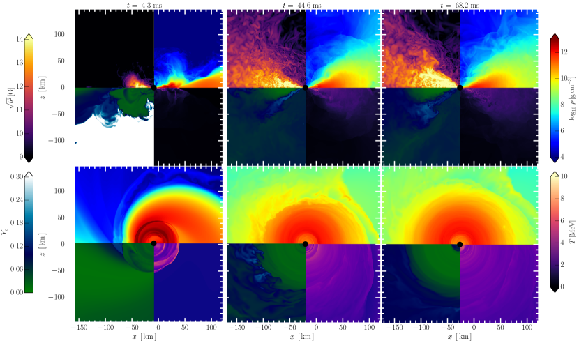
Figure 1: Model TNT.chit.0.35. Shown are the co-moving magnetic energy density $b^{2}$, the rest-mass density $\rho$, the electron fraction $Y_{e}$ and the local fluid temperature $T$. The different rows correspond to meridional (Top) and equatorial (Bottom) views of the accretion disk around the BH. The columns correspond to different times after merger, starting from the early formation of the disk after the star has been tidally disrupted (left column). The centre and right columns then refer to two times where the disk grows due to fall-back accretion of the bound tidal arm, and the onset of a steady accretion flow.

2.1 Numerical methods

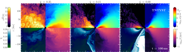
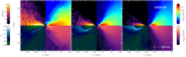
Figure 2: Shown are the evolution of the co-moving magnetic energy density $b^{2}$, the rest-mass density $\rho$, the electron fraction $Y_{e}$ and the local fluid temperature $T$ in the meridional plane. The top row shows models computed using the TNTYST EOS, while the bottom row the BHB$\Lambda\Phi$ EOS. All results are shown at $\simeq 100\,\rm ms$ after merger.

In order to model the dynamical evolution of the BH-NS system, we solve the general-relativistic ideal magnetohydrodynamics (GRMHD) equations together with the Einstein field equations (EFE),

$$\nabla_{\mu}T^{\mu\nu} =-\mathcal{Q}^{\nu}\,,$$ (1)

$$R_{\mu\nu} =8\pi\left(T_{\mu\nu}-\frac{1}{2}g_{\lambda\kappa}T^{\kappa\lambda}g_{\mu\nu}\right)$$

$$+2\nabla_{\left(\mu\right.}Z_{\left.\nu\right)}+\kappa_{1}\left[2n_{\left(\mu\right.}Z_{\left.\nu\right)}-n_{\alpha}Z^{\alpha}g_{\mu\nu}\right]\,,$$ (2)

where $g_{\mu\nu}$ is the four-dimensional Lorentzian spacetime metric, $R_{\mu\nu}$ the corresponding Ricci tensor and $T_{\mu\nu}$ the energy momentum tensor describing the NS matter and the magnetic fields.

The source term $\mathcal{Q}^{\nu}$ represents the energy and momentum loss due to weak interactions. Using the unit normal vector $n_{\mu}$ of the 3+1 slicing of the spacetime (Gourgoulhon, 2012) and the Z-vector $Z_{\mu}$ within the Z4 system (Bona et al., 2003), the EFE are written as a system that allows for the propagation of numerical constraint violations of the Einstein system (Gundlach et al., 2005). We solve the EFE using the Z4c formulation (Hilditch, 2013; Bernuzzi & Hilditch, 2010), which is a conformal variant of the Z4 system (Bona et al., 2003) (see also Alic et al. 2012). Different from Weyhausen et al. (2012), we find that simulations of BH-NS binaries employing the excision formalism on the initial data require additional damping, $\kappa_{1}=0.07$, whereas larger damping leads to instabilities of the spacetime evolution. In addition, we find it beneficial to remove the advection part in the shift condition, which is then given by (Alcubierre et al., 2003; Etienne et al., 2008),

$$\partial_{t}\beta^{i} =B^{i}\,,$$ (3)

$$\partial_{t}B^{i} =\frac{3}{4}\bar{\Gamma}^{i}-\eta B^{i}\,,$$ (4)

with damping parameter $\eta=1.4$.

The ideal-GRMHD equations (Duez et al., 2005; Shibata & Sekiguchi, 2005; Giacomazzo & Rezzolla, 2007) are supplemented by an evolution equation for the magnetic vector potential in the ideal-MHD limit (Del Zanna et al., 2003; Etienne et al., 2010). We additionally impose the Lorenz gauge for the vector potential (Etienne et al., 2012a). Neutrino losses are incorporated using a simplified leakage prescription (Ruffert et al., 1996; Rosswog & Liebendörfer, 2003; Galeazzi et al., 2013), that is appropriate for the low temperatures reached in the tidal disruption of a NS (Deaton et al., 2013; Kyutoku et al., 2018).

These equations are solved using the Frankfurt/IllinoisGRMHD code (FIL) (Most et al., 2019b; Most et al., 2019a). Although FIL is derived from the IllinoisGRMHD code (Etienne et al., 2015), it makes use of a fully fourth-order conservative finite-difference algorithm to discretize the hydrodynamical and electromagnetic flux terms (Del Zanna et al., 2007). Furthermore, it provides routines to use tabulated finite-temperature EOSs and can evolve the electron fraction $Y_{e}$. In addition, FIL solves the Z4c system using fourth-order accurate upwinded finite-differences (Zlochower et al., 2005). Details on the implementation and accuracy of the code can be found in Most et al. (2019b).

FIL is built on top of the Einstein Toolkit (Loeffler et al., 2012; Babiuc-Hamilton et al., 2019). As such, FIL uses a fixed-mesh box-in-box refinement provided by Carpet (Schnetter et al., 2004). Specifically, we use nine nested Cartesian boxes each at doubling resolution. The outer domain extends to $\simeq 6000\,\rm km$ in each direction and the initial compact objects are covered by the two finest domains with a size of $17.7\,\rm km$ and a resolution of $\simeq 215\,\rm m$. Additionally, we impose reflection symmetry along the vertical $z-$direction.

3 Results

In this work, we study the merger and post-merger evolution of near equal-mass BH-NS binaries. Before turning to the properties of the accretion disks formed in such mergers, we first provide a very brief overview of their formation. We do this by considering the fiducial system TNT.chit.0.35. In order to illustrate the disk formation process, we begin by summarizing the dynamical formation of the disk in Fig. 1, which reports the co-moving magnetic energy density $b^{2}$, the rest-mass density $\rho$, the electron fraction $Y_{e}$ and the local fluid temperature $T$. The different rows correspond to meridional (top panels) and equatorial (bottom panels) views of the accretion disk around the BH, while the different columns correspond to different times after the merger. The general dynamics of this process have been studied extensively in purely hydrodynamical simulations (Etienne et al., 2009; Kyutoku et al., 2011; Foucart et al., 2012). In order for a massive disk to form during and after merger, tidal disruption has to occur outside of the innermost stable circular orbit (ISCO) of the BH (Pannarale et al., 2011b; Shibata & Taniguchi, 2011). Starting from the left panel, we can see that shortly after tidal disruption, an initial accretion disk begins to form around the BH. Originating from the cold NS matter, the initial disk is very neutron rich ($Y_{e}<0.05$), but already reaches temperatures $T\lesssim 10\,\rm MeV$. The disk quickly grows in mass and size due to fall-back accretion from the tidal arm (middle column), begins to circularize and a steady accretion flow develops over time. As expected, this happens on the dynamical timescales of the disks, which are proportional to the disk mass $M_{\rm disk}^{b}$, so that the lightest disks circularize first. Initially, the pure neutron matter is far out of beta-equilibrium under these conditions and will rapidly re-equilibrate via beta decay of neutrons, leading to an increasing protonization especially of the low-density parts of the disk. At the same time, the magnetic-field strength is increasing throughout the disk, exceeding $10^{14}\,\rm G$ locally. More details on the magnetic-field evolution will be given in Sec. 3.3. Finally, after more than $50\,\rm ms$ past merger, the disk has settled into an initial quasi-equilibrium, consisting of a very neutron-rich disk, probing rest-mass densities $\lesssim 10^{11}\,\rm g\,cm^{-3}$. A disk formed by this process will then set the initial conditions for the long-term evolution in terms of the accretion flow and mass ejection (Fernández et al., 2015; Fernández et al., 2017).

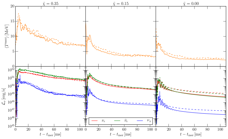
Figure 3: Temperature evolution and neutrino emission of the disk. (Top) time-averaged maximum temperature $\langle T^{\max}\rangle$. (Bottom) neutrino luminosity $\mathcal{L}_{\nu}$. Results are shown for simulations with the TNTYST (solid) and BHB$\Lambda\Phi$ EOSs. The columns represent the different models in terms of their effective spin $\tilde{\chi}$

3.1 Disk properties

One of the most important observables of such a gravitational-wave event would be the associated optical counterparts, in particular the kilonova afterglow (see Metzger, 2017, for a review). In the case of a BH–NS merger with a massive remnant accretion disk, this will be caused primarily by secular (essentially magnetically and neutrino driven) disk mass ejection (Fernández & Metzger, 2013; Fernández et al., 2015; Siegel & Metzger, 2017). In addition, dynamical mass ejection will also lead to an early red kilonova component (Kyutoku et al., 2013; Kyutoku et al., 2015; Foucart et al., 2013b; Kawaguchi et al., 2016). Previous simulations of realistic (e.g., Fernández et al. (2017); Nouri et al. (2018)) or idealised (e.g., Siegel & Metzger (2017); Fernández et al. (2019)) remnant disks have shown that a large fraction of the disk material will become unbound. Therefore, it is important to understand the initial structure of realistic disks formed during merger by the tidal disruption of the NS.

3.1.1 General observations

In this section we will focus on the composition of the disk formed after the merger and will highlight part of its evolution. As discussed in in the previous section using Fig. 1, the disk is formed by the tidal disruption of the NS at merger. The neutron-rich debris then forms an accretion disk, which will become quasi-stationary once the fall-back accretion of matter from the bound part of the tidal tail has ceased. Generically, we find that this happens after roughly $50-70\,\rm ms$.

Having outlined the general stages of the disk formation process, we now present the resulting disks for three different effective spins $\tilde{\chi}:=\chi_{\rm 1}/(1+q)=\left[0.00\,,0.15\,,0.35\right]$ of the binary, performed with both the TNTYST and BHB$\Lambda\Phi$ EOS. In Fig. 2 the rest-mass density $\rho$, electron fraction $Y_{e}$ and temperature $T$ are shown on the equatorial plane for the three effective spins at a time $t\approx 100\,\rm ms$ after merger.

We begin by discussing the evolution of the TNTYST systems (top row), although all conclusions will essentially also hold for the BHB$\Lambda\Phi$ EOS, as can be seen from the bottom row of Fig. 2. This is because the smaller compactness $C=M/R$ of the initial NS for the BHB$\Lambda\Phi$ EOS only leads to an enhancement in the disk mass (Foucart, 2012), consistent with the fact that different EOSs will affect mostly the amount of remnant disk mass, but hardly the spin of the BH or the low-density part of the EOS (Timmes & Swesty, 2000) probed in the accretion disk. Tidal disruption depends on the mass ratio and spin of the BH (Shibata & Taniguchi, 2008) (see also Shibata & Taniguchi (2011) for a review). More precisely, depending on the different effective spins of the BH (and hence also mass ratios), tidal disruption can be enhanced in our set of models (Most et al., 2020a). Indeed, we find that spin enhances the disk mass as expected from previous studies (Foucart et al., 2018), creating the most extended and massive disk for the high-spin system (left panel), with a mass $M^{\rm disk}_{b}=0.17\,M_{\odot}$ (see Tab. 1). At the same time, the zero-spin system TNT.chit.0.00 only reaches disk masses of $M^{\rm disk}_{b}=0.01\,M_{\odot}$. Interestingly, the intermediate case with effective spin $\tilde{\chi}=0.15$ features the highest rest-mass densities of all cases. The magnetic-field strength is highest in the high-spin case, and lowest in the case of zero BH spin. A more detailed discussion of the magnetic-field evolution will be given in Sec. 3.3. The temperature, $T$, also increases monotonically with spin, albeit in all cases the disks are rather cold $T\lesssim 10\,\rm MeV$, and cooling over time.

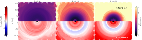
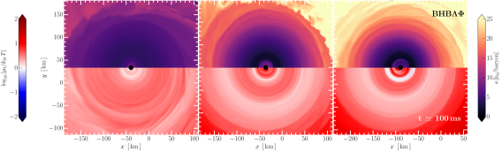
Figure 4: Equatorial view of the entropy $s$ per baryon and the lepton chemical potential $\mu_{\rm l}$, relative to the fluid temperature $T$. The top row shows models computed using the TNTYST EOS, the bottom row BHB$\Lambda\Phi$ models. All results are shown at $\simeq 100\,\rm ms$ after merger.

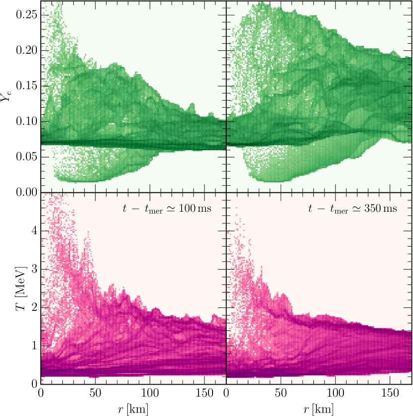
Figure 5: Electron fraction $Y_{e}$ (top panels) and temperature $T$ (bottom panels) sampled as a function of the cylindrical radius $r$ at two times after the merger. Shown are results for model TNT.chit.0.35.

The continued emission of neutrinos leads to a rapid cooling of the disk, which is shown in Fig. 3. Different from the collision of two NSs, where the compression at merger can produce very high temperatures $\gg 10\,\rm MeV$ (Perego et al., 2019; Endrizzi et al., 2020), tidal disruption is not able to significantly heat up the baryonic matter in the simulation. In fact, when comparing the different evolutions of the hottest fluid elements in the simulation domain (top panels of Fig. 3), we find that, at most, temperatures of $15\,\rm MeV$ are reached in the case of TNT.chit.0.35 and about $10\,\rm MeV$ in the lower spin cases. Neutrino emission then leads to a rapid cool-down of the disk to below $10\,\rm MeV$ on a timescale of about $\sim 50\,\rm ms$. The magnitude of neutrino luminosity from the disk is also less for the low-spin models (bottom panels of Fig. 3), consistent with the disks being colder. In all cases the initial neutrino luminosity is at least $10^{50}\,{\rm erg\,s^{-1}}$.

We can further see in Fig. 2 that the “funnel” region is mildly polluted with neutron-rich matter, except in the case of low-spin TNTYST models, which feature lower densities at higher electron fraction. This likely indicates that this matter is closer to beta-equilibrium which corresponds to more symmetric matter at those densities.

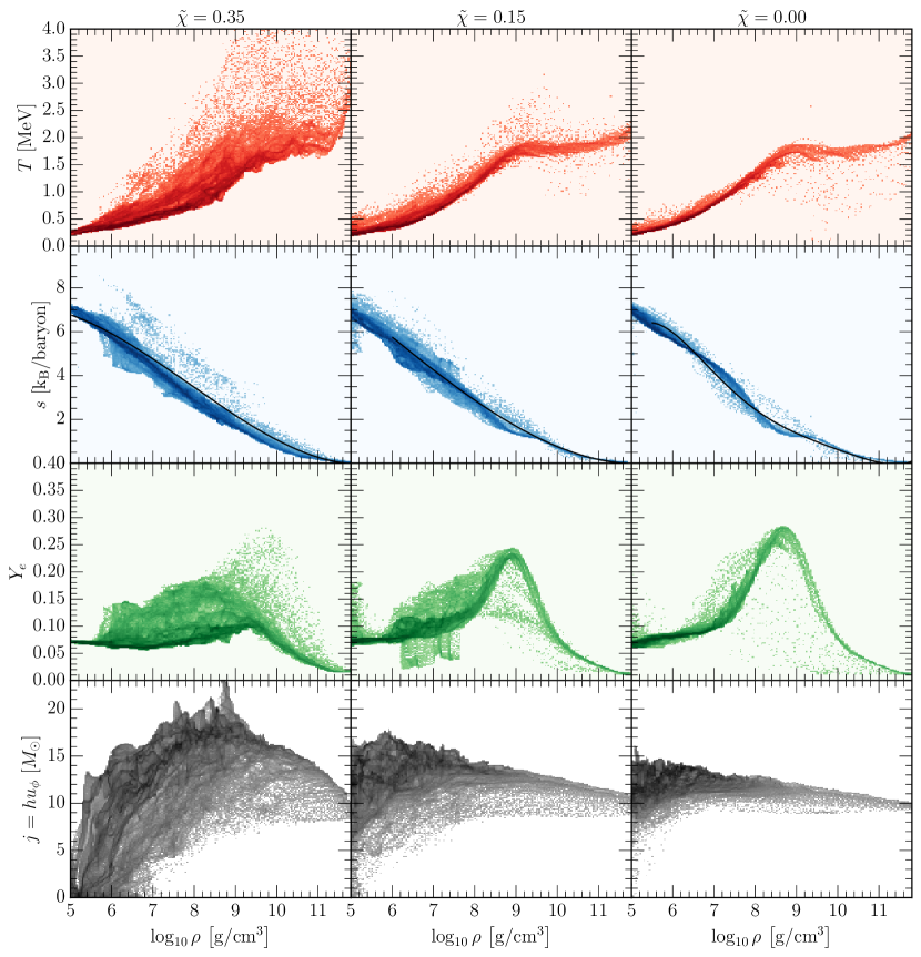
Figure 6: Properties of the accretion disks formed in BH – NS merger simulations using the TNTYST EOS for different effective spins $\tilde{\chi}$ at the same time as in Fig. 2 ($t-t_{\rm mer}\simeq 100\,\rm ms$). Shown are the temperature $T$, specific entropy per baryon $s$, electron fraction $Y_{e}$ and specific angular momentum $j:=hu_{\phi}$ sampled based on their local rest-mass density $\rho$.

3.1.2 Nuclear composition and weak-interactions

When looking at the nuclear composition of the disks, in terms of the electron fraction $Y_{e}$, we can see that the disks become more neutron rich with increasing effective spin. Furthermore, the disks begin to rapidly protonize in the outer layers, since these are transparent to neutrino emission. This can easily be understood when considering that the disks, initially formed from almost pure neutron matter in the tidal disruption process, have a composition that is far from beta-equilibrium under the post-merger conditions. Hence, beta-decay will lead to an increase in the proton–neutron ratio in the disk, that is accompanied by an emission of neutrinos. Quantitatively, this leads to an increase in the electron fraction which easily reaches $Y_{e}\simeq 0.2-0.3$. While this is most pronounced for the medium and zero spin cases (right and middle columns in Fig. 2), we expect that on larger time and lengthscales the disk in the highest-spin case (left column) will exhibit a similar behaviour.

This effect has been closely investigated by De & Siegel (2020), who found that starting with constant specific angular momentum and specific entropy disk equilibria, low-mass disks protonize more quickly and that weak interactions switch-off in these disks. Different from these idealized accretion disks, we find that the protonization is not highest in the center around the BH but largely affects a ring of low-density material. In Fig. 4 the spatial distribution of the specific entropy $s$ and the lepton chemical potential $\mu_{\rm l}$ is reported, for which the latter tends to zero in beta-equilibrium. Indeed, this proton-rich ring quickly beta-equilibrates (blue regions), as $\mu_{\rm l}/k_{B}T\ll 1$. Interestingly, we find that in the case of the $\rm BHB\Lambda\Phi$ models (bottom row) an inner ring of matter close to beta-equilibrium develops, whereas the outer ring is less equilibrated than in the TNTYST cases. This inner ring is seemingly absent for models with the TNTYST EOS (top row). Moreover, we find that our realistic remnant accretion disks feature density-dependent variations of the specific entropy, $s<10$.

To complete our discussion on weak interactions in the disk, we briefly point out the presence of disk self-regulation (Chen & Beloborodov, 2007; Siegel & Metzger, 2017), following the discussion in Siegel & Metzger (2018). While Fig. 4 would imply that large parts of the disk are out of beta-equilibrium and would have to protonize, self-regulation at the inner edge of the disk, will lead to neutronization that maintains $Y_{e}\simeq 0.1$. This is because in this neutrino transparent regime copious $e^{\pm}$-pair production will effectively modify the beta-equilibrium condition (Beloborodov, 2003). The balance between turbulent heating (induced by the magneto-rotational instability, see Sec. 3.3) and neutrino cooling will then establish this reservoir of neutron-rich matter in the inner edge of the disk.

Although this study primarily focusses on obtaining initial conditions for disks after tidal disruption, our long-term simulation (TNT.chit.0.35), was run long enough to exhibit this behaviour. Indeed, as shown in the top panels of Fig. 5, the disk is initially (i.e., at $t-t_{\rm mer}=100\,\rm ms$) very neutron rich with $Y_{e}<0.15$, since it was formed from the neutron-rich matter of the tidal disrupted NS. However, at the final time of our simulation (i.e., at $t-t_{\rm mer}=350\,\rm ms$), large parts of the disk have already begun to protonize, reaching $Y_{e}\simeq 0.2$ at larger distances $r>80\,\rm km$ from the BH, where densities are larger and the cooling less effective. We can also see this by looking at the temperature profiles in the bottom panels of Fig. 5. More specifically, at later times while the main part of the disk cools only slowly, close to the BH and at distances $r<40\,\rm km$, where the densities are smaller and the cooling is more effective, most of the disk matter is even more neutron rich than initially, i.e., having $Y_{e}<0.1$. This is consistent with the onset of self-regulation and broadly agrees with the findings presented in Siegel & Metzger (2018).

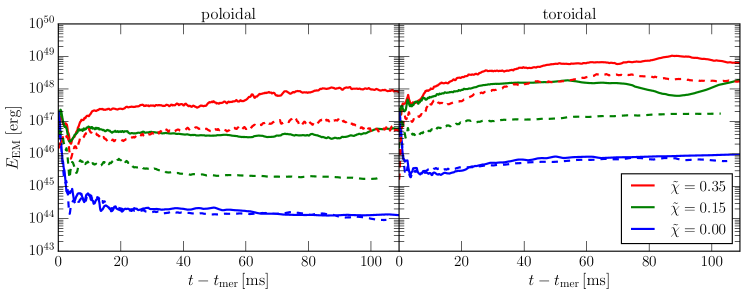
Figure 7: Evolution of the magnetic energy, $E_{\rm EM}$, after the merger at time $t_{\rm mer}$. Shown are the total poloidal (left) and toroidal component (right). The colors refer to the different models in terms of their effective spins, $\tilde{\chi}$. Solid lines represent simulations with the TNTYST and dashed lines with the BHB$\Lambda\Phi$ EOSs.

3.2 Bulk hydrodynamic properties

We now focus on the hydrodynamic properties of the accretion disk. When constructed as equilibrium configurations in axisymmetry (Fishbone & Moncrief, 1976), accretion disks are usually described in terms of the specific angular momenta $j$, specific entropies $s$, disk masses $M_{\rm disk}$, and their electron fractions $Y_{e}$. Typically, those are assumed to be constants in most previous studies (e.g. Siegel & Metzger (2017); Fernández et al. (2019)). Having a set of fully consistent GRMHD simulations of accretion disks formed by tidal disruption in the merger of BH–NS systems, does in fact allow us to compute realistic distributions of the above fluid quantities as functions of the rest-mass density $\rho$. These are shown in Fig. 6 for simulations using the TNTYST EOS. Starting from the top, we first show the temperature distributions that, in all of the three cases, exhibit a flat plateau around $T\simeq 2\,\rm MeV$, which changes to a fall-off for rest-mass densities $\rho<10^{9}\,\rm g\,cm^{-3}$. The entropy profiles (second row from the top) are almost linear in all cases, starting from specific entropies $s<1$ at the highest densities and extending outwards until $s\approx 7-8$ for the lowest densities in the disks, $\rho\simeq 10^{5}\,\rm g\,cm^{-3}$. Interestingly, low-mass disks, i.e., obtained for $\tilde{\chi}=\left[0.00\,,0.15\right]$, seem to feature a small plateau around $\rho\simeq 10^{9}\,\rm g\,cm^{-3}$, corresponding roughly to the transition to the nuclear statistical equilibrium EOS used at low densities. Overall, it is possible to provide an effective fit for the specific entropy in terms of the function

$$s=\sum_{k=0}^{5}c_{k}\left(\log_{10}\left[\rho/\left(\rm g\,cm^{-3}\right)\right]\right)^{k}\,.$$ (5)

where the numerical values for the coefficients $c_{k}$ are provided in Tab. 2.

	$c_{0}$	$c_{1}$	$c_{2}$	$c_{3}$	$c_{4}$	$c_{5}$	$n_{\rm P}$	$n_{\rm T}$
TNT.chit.0.00	$-2.87\times 10^{2}$	$1.81\times 10^{2}$	$-4.32\times 10^{1}$	$5.01$	$-2.85\times 10^{-1}$	$6.41\times 10^{-3}$	$0.63$	$0.81$
TNT.chit.0.15	$1.32\times 10^{1}$	$-5.15\times 10^{-1}$	$-1.92\times 10^{-1}$	$1.19\times 10^{-2}$	$-$	$-$	$0.60$	$0.83$
TNT.chit.0.35	$1.27$	$3.50$	$-6.09\times 10^{-1}$	$2.56\times 10^{-2}$	$-$	$-$	$0.68$	$0.81$
BHB.chit.0.00	$-2.21\times 10^{2}$	$1.44\times 10^{2}$	$-3.53\times 10^{1}$	$4.17$	$-2.42\times 10^{-1}$	$5.53\times 10^{-3}$	$0.67$	$0.87$
BHB.chit.0.15	$2.21\times 10^{1}$	$-3.16$	$6.72\times 10^{-2}$	$3.55\times 10^{-3}$	$-$	$-$	$0.77$	$0.97$
BHB.chit.0.35	$8.39$	$1.39$	$-4.15\times 10^{-1}$	$2.03\times 10^{-2}$	$-$	$-$	$0.67$	$0.87$

Table 2: Numerical coefficients for the fits of the specific entropy $s$ and magnetic-field strengths $B_{\rm P,T}$. See Eqs. (5) and (6) for details.

Focussing on the electron fraction $Y_{e}$, we can continue our earlier discussion around Fig. 4, where a ring-like structure in the disk approaching beta-equilibrium is observable. Looking at $Y_{e}\left(\rho\right)$ (third row from the top in Fig. 6), we can see that the bulk of the matter in the disk follows a tight relation with the rest-mass density. The innermost, densest parts of the disk, i.e., $\rho>10^{10}\,\rm g\,cm^{-3}$, are at very low electron fractions, $Y_{e}<0.05$, thus implying that most of the disk is made of almost pure neutron matter. Moving outwards to lower densities and approaching the beta-equilibrated ring (for $\tilde{\chi}=0.00,0.15$), the electron fraction peaks at $Y_{e}=0.25$ for densities around $\rho=10^{9}\rm\,g\,cm^{-3}$. Instead of continuing to increase as would be predicted in beta-equilibrium, the electron fraction decreases again to below $Y_{e}<0.1$. For the highest-spin case, the situation is slightly different. We can see that a small fraction of the disk material exhibits a similar (beta-equilibrated) $Y_{e}$-peak as in the other cases, but most of the disk remains at electron fractions $Y_{e}<0.1$, indicating that the entire disk remains neutron rich. This is consistent with the weak-interaction “ignition threshold” proposed by De & Siegel (2020).

Concerning the specific angular momentum that governs the structure of the disk (bottom row), we find that depending on the effective spin $\tilde{\chi}$ and, hence, on the disk mass, the distributions look very different. Although there are different definitions of the relativistic angular momentum $j$ in use in the literature (Kozlowski et al., 1978), we have found only minor differences between them when extracted from our simulations. For simplicity, we therefore choose to adopt the one used for massive disks $j:=hu_{\phi}$, where $h$ is the specific enthalpy and $u_{\phi}$ the covariant azimuthal-component of the fluid four-velocity (Kiuchi et al., 2011). For the highest disk mass and spin (left panel), we find for large parts of the disk, $\rho>10^{8}\,\rm g\,cm^{-3}$, that the specific angular momentum is far from being constant, as customarily assumed in simplified models of equilibrium tori. Rather, the specific angular momentum varies in the range $10<hu_{\phi}/M_{\odot}<20$, and decreases further out at low densities $<10^{8}\,{\rm g\,cm^{-3}}$ as required by dynamical stability. Only for lower spins and disk masses, can the specific angular momentum be considered closer to a constant, although also in this case it ranges from $10<hu_{\phi}/M_{\odot}<15$.

In comparison, Fig. 13 in Appendix A, shows the same distributions but for the mergers using the BHB$\Lambda\Phi$ EOS. While the temperature, entropy and electron fraction distributions look overall very similar, the angular momentum distributions are different. For high and medium spin (left and middle panel, bottom row), the results do look comparable, but the zero-spin case features a split of the specific angular momentum in two semi-constant branches.

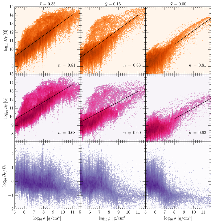
Figure 8: Density-dependent distributions of the poloidal, $B_{\rm P}$, and toroidal, $B_{\rm T}$, components of the magnetic field at the same time as in Fig. 2 ($t-t_{\rm mer}\simeq 100\,\rm ms$). The simulations shown use the TNTYST EOS and $n$ is defined in Eq. (6).

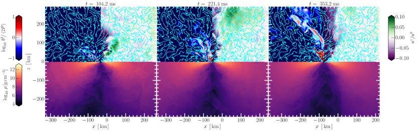
Figure 9: Long-term evolution of the TNTYST.chi.035 system. The top half shows the vertical flow velocity $u^{z}/u^{0}$ and the inverse plasma parameter $\beta:=b^{2}/\left(2p\right)$, computed in terms of the comoving magnetic energy density $b^{2}$ and of the fluid pressure $p$. The lower half of the panel shows the rest-mass density $\rho$. The magnetization of the funnel is steadily growing over time (red regions), while the matter inside the funnel is increasingly inflowing (violet regions), indicating potential funnel clearing on longer timescales.

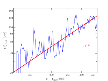
Figure 10: Characteristic scale-height of the magnetized funnel region, where $\langle z\rangle_{\beta=1}$ refers to the average vertical height corresponding to the plasma parameter $\beta=b^{2}/\left(2p\right)=1$. The time is measured relative to the time of merger $t_{\rm mer}$.

3.3 Magnetic-field evolution

While the disk is cooling, the dynamics of the plasma and magnetic instabilities lead to an increase in the magnetic field strength, as shown in Fig. 7, which displays the evolution of the toroidal and poloidal magnetic energy. Note that after the merger, the disruption of the NS leads to a shearing of the magnetic-field lines in its interior, which causes a sudden amplification of the magnetic field (Rezzolla et al., 2011; Etienne et al., 2012b). Because of the geometry of the disruption event, the amplification will mainly affect the toroidal component of the field. The predominantly poloidal parts of the magnetic fields in the center of the disrupted star experience a smaller amplification and are mostly accreted by the BH, as can be seen by the sudden drop in poloidal energy directly after merger (left panel). In the case of the zero-spin binary TNT.chit.0.00, almost the entire NS is accreted and only the weakly magnetized matter in the outermost parts of the original NS remain to form the disk. This is accompanied with a very sharp drop in both components of the magnetic energy. After the merger the magnetorotational instability (MRI) (Velikhov, 1959; Chandrasekhar, 1960; Balbus & Hawley, 1991) will begin to drive an early amplification of the magnetic field, which can be seen by an increase in both poloidal and toroidal field components. A key feature to accurately capture this amplification is with the use of a fourth-order accurate numerical scheme (Most et al., 2019b), which helps to resolve instabilities, such as the MRI, even at lower resolutions in the outer parts of the disk. The use of such schemes can, however, not alleviate the need for resolving the lengthscales associated with physical processes and instabilities. Indeed, we find that the lowest mass disk, case TNT.chit.0.00, leads to a disk of roughly half the size of the other cases, pointing to the need for higher resolutions than we currently employ. The absence of poloidal field growth for this case confirms that the MRI wavelength is not fully resolved in large parts of the disk and that the MRI is likely not active in this simulation. Given the low mass of the disk and the low observational prospects, we choose to not repeat this calculation at higher resolution.

Comparing the evolution of the magnetic energy for different BH spins, we find that the high-spin cases feature larger magnetic energies, with the models with the TNTYST EOS (solid curves), having up to an order of magnitude higher electromagnetic energies than the BHB$\Lambda\Phi$ models (dashed curves). This already points to a mild EOS dependence on the subsequent disk evolution. Moreover, we can already anticipate that the magnetic-field geometry is largely toroidal by comparing the left and right panels in Fig. 7. Since the initial structure of the field geometry might critically affect the timescales of the late-time evolution of the disk (Christie et al., 2019), we next present a detailed analysis of the magnetic-field topology.

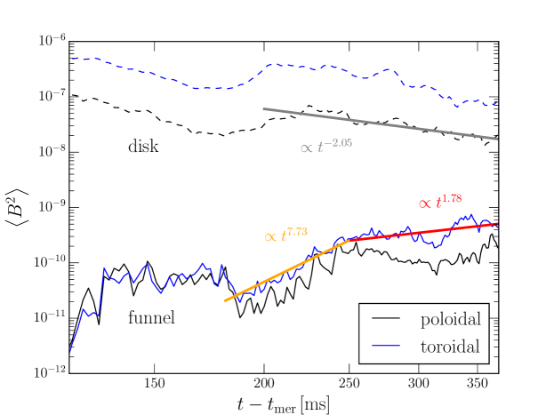
Figure 11: Evolution of the mean magnetic energy density, $\langle B^{2}\rangle$, in terms of poloidal (black) and toroidal (blue) components. The evolution is shown separately for the disk (dashed lines) and for the funnel region (solid lines). The time is measured relative to the time of merger $t_{\rm mer}$.

3.4 Magnetic-field topology

We can further investigate the structure and properties of the magnetic field by looking at density distributions of the poloidal $B_{\rm P}$ and toroidal $B_{\rm T}$ magnetic-field components, as shown in Fig. 8 for the simulations using the TNTYST EOS. Starting from the irrotational case, $\tilde{\chi}=0.00$ (left column), we can see that, overall, the bulk of the poloidal and toroidal fields follows a power-law dependence with the rest-mass density

$$\log_{10}\left[B_{\rm P,T}/{\rm G}\right]=n_{\rm P,T}\log_{10}\left[\rho/\left({\rm g\,cm^{-3}}\right)\right]+\rm const.\,,$$ (6)

where the values of the two coefficients $n_{\rm P,T}$ are reported in Tab. 2.

Note that the toroidal magnetic field peaks at $10^{14}\,G$. The poloidal to toroidal ratio is $B_{\rm P}/B_{\rm T}\simeq 0.1$, and increases locally to $B_{\rm P}/B_{\rm T}\lesssim 10$ for low rest-mass densities $\rho<10^{7}\,\rm g\,cm^{-3}$. This is mainly due to the appearance of the MRI, which causes a sustained replenishing of the poloidal field (Sa̧dowski et al., 2015). Conversely, this also confirms our initial conclusion that the MRI is likely not resolved in the least massive and, hence, smallest of the disks. While this clearly indicates that any subsequent evolution of this disk at current resolution is not feasible, it also allows us to draw an important conclusion about the correct initial conditions for the magnetic field. Namely, that the profiles seen in the third column of Fig. 8 should be indicative for realistic initial magnetic-field topologies in disks formed directly in BH-NS mergers. Since the subsequent magnetic-field evolution is very modest, these distributions represent the initial magnetic-field configuration in the disk as soon is it equilibrates after merger. More importantly, these distributions are rather different from those normally employed in simulations starting from axisymmetric tori in equilibrium, which often even ignore the presence of a toroidal component.

This qualitative behaviour described before is the same for all disks. However, the larger poloidal-toroidal ratio is indicative of the fact that the MRI is active in increasingly larger parts – and at higher densities – of the disks. For the high-spin case, $\tilde{\chi}=0.35$, we can clearly see that the MRI is active throughout the disk and that both poloidal and toroidal field grow beyond the simple power-law behaviour outlined before. Looking at the corresponding Fig. 14 in Appendix A, it is possible to deduce that this behaviour holds also for a different EOS, and that the overall magnitude of the magnetic field remains insensitive to the initial choice of EOS for the inspiraling NS. Nonetheless, the slope coefficients $n_{\rm P,T}$ are slightly larger when compared to the simulations with the TNTYST EOS. Although this change is rather minor, it does hint that the slightly altered distribution of the magnetic field inside the initial NS is partially imprinted onto the disk, as it would be natural to expect.

3.5 Prospects of jet launching

Having discussed the composition structure of the disk and the magnetic field topology present in the accretion disks formed in (low-mass) BH–NS mergers, we now turn to the prospect of launching a jet from these systems. While this process has been thoroughly studied for accretion disks found in supermassive BH accretion (Abramowicz & Fragile, 2013; Porth et al., 2019; Davis & Tchekhovskoy, 2020), only a few attempts have been made in the context of NS mergers, both in ideal (Rezzolla et al., 2011; Paschalidis et al., 2015; Kiuchi et al., 2015; Kawamura et al., 2016; Ruiz et al., 2018b) and resistive MHD Dionysopoulou et al. (2015); Qian et al. (2018). Unless an external field was initially seeded by means of a force-free like magnetosphere (Paschalidis et al., 2015; Ruiz et al., 2020), most simulations have only observed the formation of a helical magnetic-field structure in the funnel region (Kawamura et al., 2016), however, not an actual (relativistic) outflow. In most cases, strong baryon pollution from the disk created large ram pressures preventing the funnel from clearing and attaining a magnetically dominated, force-free state Kiuchi et al. (2014, 2015). Since most of these simulations were run with low resolutions and for short timescales $\lesssim 100\,\rm ms$, it currently remains an open problem to understand under what conditions the magnetization in the funnel would grow over longer timescales. Recent simulations of accretion disks with toroidal magnetic fields indeed indicated that the timescale for magnetic-field growth is significantly longer than for initial poloidal geometries typically used to study jet launching (Liska et al., 2018; Christie et al., 2019). While these studies benefit from having higher resolutions close to the BH horizon, due to the use of better suited spherical coordinate systems, the use of a fully fourth-order numerical scheme allows us to accurately capture magnetic instabilities in the disk with fewer grid points than needed for second-order codes (Most et al., 2019b). Therefore, we evolve one of the systems TNTYST.chi.035 until $\sim 350\,\rm ms$ in order to gauge its prospect for jet launching. Since the BH retains a net linear momentum after merger, we continue to solve the Einstein equations alongside those of GRMHD.

In Fig. 9 we report the evolution of the funnel region in terms of plasma parameter $\beta^{-1}:=b^{2}/\left(2p\right)$ – where $b^{2}$ is the comoving magnetic energy density and $p$ the fluid pressure – and the vertical flow velocity $u^{z}/u^{0}$. Note that while the funnel starts out being only weakly magnetized (left panel), the magnetization grows steadily over time with increasingly larger portions exhibiting $\beta^{-1}>1$ (middle and right panels) in the polar regions above the BH (funnel). The projected magnetic-field lines indicate a twistor shape field geometry as observed previously by Kawamura et al. (2016). At the same time, the funnel regions begins to evacuate on essentially the same timescale. A steadily increasing inflow, indicated by the dark violet regions in Fig. 9, strongly hints to an eventual clearing of the funnel, although large patches are still strongly polluted by disk inflows (lower half of the panels). In order to better quantify the growing magnetization of the funnel, we introduce a characteristic scale-height $\langle z\rangle_{\beta=1}$, which corresponds to the average $z$-coordinate with the plasma parameter $\beta=1$. This parameter may be interpreted as a proxy for how the magnetization of the funnel varies in the vertical direction. We caution that a fully force-free funnel would require $\beta\ll 1$, although such values will in practice not be present until shortly before jet launching. We show the corresponding evolution of the scale-height in Fig. 10. Although there are inherent fluctuations over time, on average we find that the magnetization scale-height is constantly growing with a power law $\langle z\rangle_{\beta=1}\propto t^{\alpha}$, with $\alpha=1.78$. At the end of our simulation, this scale-height extends to about $140\,\rm km$. If this growth was sustained at the same rate, the scale-height would double around $\simeq 500\,\rm ms$. Since the rest-mass densities decrease at larger distances from the BH, it might be possible for this growth to accelerate at sufficient distance from the BH, due to the faster decrease in pressure in those regions.

In order to better understand this behaviour, we have performed a detailed analysis of the magnetic-field topology in the funnel and the disk. To be more precise, we have computed mean magnetic-field energy densities $\langle B^{2}\rangle$ for the toroidal and poloidal components in the funnel and in the disk. We define the funnel region simply in terms of density and angular cut-offs. More specifically, we define the funnel to be within $30^{\circ}$ from the polar axis and contain densities of at most $10^{9}\,\rm g\,cm^{-3}$. The resulting evolution is shown in Fig. 11. We can see that initially the magnetic-field strength is not growing in the funnel region. Only after $\simeq 200\,\rm ms$, when the funnel has begun to clear we do see a rapid growth in magnetic energy following a power law with exponent $\alpha\approx 7.73$, which continues for around $50\,\rm ms$. Afterwards the growth does not stop, but continues at a lower rate. Surprisingly, it turns out that the growth is comparable to the growth of the magnetization scale-height, having an exponent $\alpha\approx 1.78$, consistent with the scaling reported in Fig. 10. At the same time the magnetic energy density in the disk is decreasing, likely because of accretion regions with strong magnetic fields in the accretion disks, which are closest to the ISCO, see Fig. 2.

Finally, we also consider the electromagnetic energy outflowing from the system. This is quantified in terms of the Poynting flux

$$\mathcal{L}_{\rm EM}=\oint T^{t}_{i\,,{\ \rm EM}}{d}S^{i}\,,$$ (7)

extracted on a spherical surface at around $500\,\rm km$ from the BH. Here $T^{\mu\nu}_{\rm EM}$ is the electromagnetic part of the stress-energy tensor (Baumgarte & Shapiro, 2003). The resulting luminosity is shown in Fig. 12. Starting at $10^{45}{\rm erg\,s^{-1}}$ at merger, the Poynting flux steadily increases and saturates at $10^{49}{\rm erg\,s^{-1}}$ after about $300\,\rm ms$.

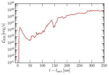
Figure 12: Electromagnetic luminosity $\mathcal{L}_{\rm EM}$ in terms of the Poynting flux for the long-term evolution of model TNTYST.chi.035. The time is measured relative to the time of merger $t_{\rm mer}$.

4 Conclusions

We have presented the results of a series of simulations in full general relativity leading to the formation of accretion disks in the aftermath of the merger of BH-NS systems in the near equal-mass regime parametrized by the maximum mass of a nonrotating NS. Including strong magnetic fields, weak interactions and realistic EOS, the disks have been evolved for $\simeq 100\,\rm ms$ after merger until a quasi-stationary disk equilibrium has been established. We have then provided a detailed comparison of the disk properties for three different disk masses and BH spins. In particular, we have found that the disks, while remaining very cold, $T\lesssim 2\,\rm MeV$, have specific-entropy distributions that follow power-laws in terms of the rest-mass density, $s\propto\rho^{-n}$. Similarly, we were able to confirm that light disks more quickly beta-equilibrate, while more massive disks remain neutron rich (De & Siegel, 2020). Importantly, massive disks have specific angular-momentum distributions that are far from being constant, as instead customarily assumed in simplified simulations starting from axisymmetric tori in equilibrium, and vary in a rather wide range. At the same time, the specific angular momentum distributions of the lighter disks have smaller ranges of variation and may be roughly approximated as constant.

We have also found that the use of different EOSs with significantly different compactnesses leads to changes in the disk mass, while the other properties of the disk seem to be largely unaffected. Having performed simulations with strong magnetic fields in the interior of the NS companion, has allowed us to examine the magnetic-field structure present in the post-merger disk when a quasi-stationarity solution is reached. While previous studies have usually superimposed poloidal magnetic fields (Nouri et al., 2018) or – more realistically – toroidal fields (Christie et al., 2019) on post-merger disks, we were able to find density-dependent scaling laws for realistic magnetic-field configurations, i.e., $B\propto\rho^{m}$. Consistent with previous simulations (Giacomazzo et al., 2011; Rezzolla et al., 2011; Kiuchi et al., 2015) and studies of binary NS mergers (Kiuchi et al., 2014; Kawamura et al., 2016), we find that the field topology is initially strongly toroidal, albeit the onset of the MRI leads to an eventual increase and amplification of the poloidal field.

Although we believe that the results presented in this work will be crucial for future modeling of post-merger accretion disks, some remarks are in order. Owing to the high computational cost of performing BH-NS mergers with accurate descriptions of the microphysics and magnetic-field evolution, we have only investigated the near equal-mass regime. While this might be most indicative for low-mass BH-NS and high-mass NS-NS mergers (see Most et al. (2020c) for a comparison), realistic BH-NS mergers are expected to happen for mass ratios $q<1/4$ (Kruckow et al., 2018). Although disk formation for these systems is largely governed by the spin of the BH (Foucart, 2012; Foucart et al., 2018), it remains to be confirmed if the magnetic-field topology and entropy profiles of the disk found here continue to hold also for these systems. Since the primary formation mechanism, i.e., tidal disruption, operates similarly in all cases, we conjecture that most likely our results should be transferable and therefore also hold qualitatively.

Finally, we have investigated the prospects of jet launching from these disks. Although we have not observed the launching of a jet, we did find strong evidence for continued funnel clearing. We have identified the characteristic funnel magnetization and clearing time scales. In particular we found that the magnetization scale-height of the funnel and the magnetic energy associated with it follow a power law, with the dominant component being $\approx t^{2}$. Interestingly, by the end of our simulation a region extending $140\,\rm km$ above the BH started to reach a strong magnetization as indicated by the plasma beta parameter approaching unity. Finally, we found that a continuous Poynting luminosity of $10^{49}\,{\rm erg\,s^{-1}}$ is driven at late times.

Future work will be required to further investigate whether jet launching is possible in these systems. Crucially, higher resolutions and longer simulation times $>1\,\rm s$ will be needed. In that context it is of particular relevance to point out that the parameter ranges found for realistic accretion disks in terms of composition, disk mass, specific entropy and magnetic-field topology can be used to initialize such simulations, thereby removing the need to perform full numerical relativity simulations to accurately study the long-term evolution of this problem.

Data availability

Data is available upon reasonable request from the Corresponding Author.

Appendix A BHB$\Lambda\Phi$ models

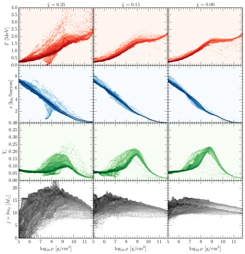
Figure 13: Same as Fig. 6 but for simulations using the BHB$\Lambda\Phi$.

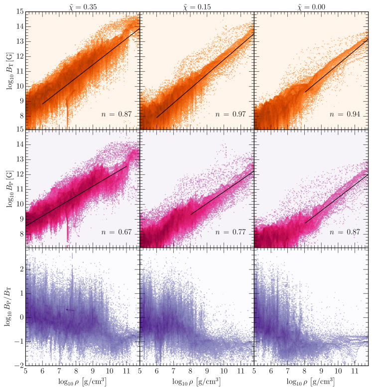
Figure 14: Same as Fig. 8 but using the BHB$\Lambda\Phi$ EOS.

In this appendix, we show the disk properties for models using the BHB$\Lambda\Phi$ EOS. In particular, Fig. 13 shows the hydrodynamical properties, whereas Fig. 14 shows the topology of the magnetic field present in the disk. These figures should be contrasted with the equivalent representations in Figs. 6 and 8, which refer instead to the TNTYST EOS (see Secs. 3.2 and 3.3 for a discussion of those results).

References

- Abbott et al. (2018) Abbott B. P., et al., 2018, Physical Review Letters, 121, 161101
- Abramowicz & Fragile (2013) Abramowicz M. A., Fragile P. C., 2013, Living Rev. Relativity, 16
- Alcubierre et al. (2003) Alcubierre M., Brügmann B., Diener P., Koppitz M., Pollney D., Seidel E., Takahashi R., 2003, Phys. Rev. D, 67, 084023
- Alic et al. (2012) Alic D., Bona-Casas C., Bona C., Rezzolla L., Palenzuela C., 2012, Phys. Rev. D, 85, 064040
- Anand et al. (2021) Anand S., et al., 2021, Nature Astronomy, 5, 46
- Annala et al. (2018) Annala E., Ecker C., Hoyos C., Jokela N., Fernández D. R., Vuorinen A., 2018, Journal of High Energy Physics, 2018, 78
- Babiuc-Hamilton et al. (2019) Babiuc-Hamilton M., et al., 2019, Zenodo
- Balbus & Hawley (1991) Balbus S. A., Hawley J. F., 1991, Astrophys. J., 376, 214
- Banik et al. (2014) Banik S., Hempel M., Bandyopadhyay D., 2014, Astrohys. J. Suppl., 214, 22
- Baumgarte & Shapiro (2003) Baumgarte T. W., Shapiro S. L., 2003, Astrophys. Journal, 585, 921
- Beloborodov (2003) Beloborodov A. M., 2003, Astrophys. J., 588, 931
- Bernuzzi & Hilditch (2010) Bernuzzi S., Hilditch D., 2010, Phys. Rev. D, 81, 084003
- Bona et al. (2003) Bona C., Ledvinka T., Palenzuela C., Zácek M., 2003, Phys. Rev. D, 67, 104005
- Caudill et al. (2006) Caudill M., Cook G. B., Grigsby J. D., Pfeiffer H. P., 2006, Phys. Rev. D, 74, 064011
- Chandrasekhar (1960) Chandrasekhar S., 1960, Proc. Natl. Acad. Sci., 46, 253
- Chawla et al. (2010) Chawla S., Anderson M., Besselman M., Lehner L., Liebling S. L., Motl P. M., Neilsen D., 2010, Phys. Rev. Lett., 105, 111101
- Chen & Beloborodov (2007) Chen W., Beloborodov A. M., 2007, Astrophys. J., 657, 383
- Christie et al. (2019) Christie I. M., Lalakos A., Tchekhovskoy A., Fernández R., Foucart F., Quataert E., Kasen D., 2019, Mon. Not. R. Astron. Soc., 490, 4811
- Davis & Tchekhovskoy (2020) Davis S. W., Tchekhovskoy A., 2020, Ann. Rev. Astron. & Astrophys., 58, 407
- De & Siegel (2020) De S., Siegel D., 2020, arXiv e-prints, p. arXiv:2011.07176
- De et al. (2018) De S., Finstad D., Lattimer J. M., Brown D. A., Berger E., Biwer C. M., 2018, Physical Review Letters, 121, 091102
- Deaton et al. (2013) Deaton M. B., et al., 2013, Astrophys. J., 776, 47
- Del Zanna et al. (2003) Del Zanna L., Bucciantini N., Londrillo P., 2003, Astron. Astrophys., 400, 397
- Del Zanna et al. (2007) Del Zanna L., Zanotti O., Bucciantini N., Londrillo P., 2007, Astron. Astrophys., 473, 11
- Dionysopoulou et al. (2015) Dionysopoulou K., Alic D., Rezzolla L., 2015, Phys. Rev. D, 92, 084064
- Duez et al. (2005) Duez M. D., Liu Y. T., Shapiro S. L., Stephens B. C., 2005, Phys. Rev. D, 72, 024028
- East et al. (2015) East W. E., Paschalidis V., Pretorius F., 2015, Astrophys. J. Lett., 807, L3
- Endrizzi et al. (2020) Endrizzi A., et al., 2020, European Physical Journal A, 56, 15
- Etienne et al. (2007) Etienne Z. B., Faber J. A., Liu Y. T., Shapiro S. L., Baumgarte T. W., 2007, Phys. Rev. D, 76, 101503
- Etienne et al. (2008) Etienne Z. B., Faber J. A., Liu Y. T., Shapiro S. L., Taniguchi K., Baumgarte T. W., 2008, Phys. Rev. D, 77, 084002
- Etienne et al. (2009) Etienne Z. B., Liu Y. T., Shapiro S. L., Baumgarte T. W., 2009, Phys. Rev. D, 79, 044024
- Etienne et al. (2010) Etienne Z. B., Liu Y. T., Shapiro S. L., 2010, Phys. Rev. D, 82, 084031
- Etienne et al. (2012a) Etienne Z. B., Paschalidis V., Liu Y. T., Shapiro S. L., 2012a, Phys. Rev. D, 85, 024013
- Etienne et al. (2012b) Etienne Z. B., Liu Y. T., Paschalidis V., Shapiro S. L., 2012b, Phys. Rev. D, 85, 064029
- Etienne et al. (2012c) Etienne Z. B., Paschalidis V., Shapiro S. L., 2012c, Phys. Rev. D, 86, 084026
- Etienne et al. (2015) Etienne Z. B., Paschalidis V., Haas R., Mösta P., Shapiro S. L., 2015, Class. Quantum Grav., 32, 175009
- Fernández & Metzger (2013) Fernández R., Metzger B. D., 2013, Mon. Not. R. Astron. Soc., 435, 502
- Fernández et al. (2015) Fernández R., Quataert E., Schwab J., Kasen D., Rosswog S., 2015, Mon. Not. R. Astron. Soc., 449, 390
- Fernández et al. (2017) Fernández R., Foucart F., Kasen D., Lippuner J., Desai D., Roberts L. F., 2017, Classical and Quantum Gravity, 34, 154001
- Fernández et al. (2019) Fernández R., Tchekhovskoy A., Quataert E., Foucart F., Kasen D., 2019, Mon. Not. R. Astron. Soc., 482, 3373
- Fishbone & Moncrief (1976) Fishbone L. G., Moncrief V., 1976, Astrophys. J., 207, 962
- Foucart (2012) Foucart F., 2012, Phys. Rev. D, 86, 124007
- Foucart et al. (2011) Foucart F., Duez M. D., Kidder L. E., Teukolsky S. A., 2011, Phys. Rev. D, 83, 024005
- Foucart et al. (2012) Foucart F., Duez M. D., Kidder L. E., Scheel M. A., Szilagyi B., Teukolsky S. A., 2012, Phys. Rev. D, 85, 044015
- Foucart et al. (2013a) Foucart F., et al., 2013a, Phys. Rev. D, 87, 084006
- Foucart et al. (2013b) Foucart F., et al., 2013b, Phys. Rev. D, 88, 064017
- Foucart et al. (2014) Foucart F., et al., 2014, Phys. Rev. D, 90, 024026
- Foucart et al. (2015) Foucart F., et al., 2015, Phys. Rev. D, 91, 124021
- Foucart et al. (2017) Foucart F., et al., 2017, Classical and Quantum Gravity, 34, 044002
- Foucart et al. (2018) Foucart F., Hinderer T., Nissanke S., 2018, Phys. Rev. D, 98, 081501
- Foucart et al. (2019) Foucart F., Duez M. D., Kidder L. E., Nissanke S. M., Pfeiffer H. P., Scheel M. A., 2019, Phys. Rev. D, 99, 103025
- Fragione & Loeb (2021) Fragione G., Loeb A., 2021, Mon. Not. R. Astron. Soc., 503, 2861
- Galeazzi et al. (2013) Galeazzi F., Kastaun W., Rezzolla L., Font J. A., 2013, Phys. Rev. D, 88, 064009
- Giacomazzo & Rezzolla (2007) Giacomazzo B., Rezzolla L., 2007, Class. Quantum Grav., 24, 235
- Giacomazzo et al. (2011) Giacomazzo B., Rezzolla L., Baiotti L., 2011, Phys. Rev. D, 83, 044014
- Gourgoulhon (2012) Gourgoulhon E., 2012, 3+1 Formalism in General Relativity. Lecture Notes in Physics, Berlin Springer Verlag Vol. 846, Springer, doi:10.1007/978-3-642-24525-1
- Grandclément (2006) Grandclément P., 2006, Phys. Rev. D, 74, 124002
- Gundlach et al. (2005) Gundlach C., Martin-Garcia J. M., Calabrese G., Hinder I., 2005, Class. Quantum Grav., 22, 3767
- Hayashi et al. (2020) Hayashi K., Kawaguchi K., Kiuchi K., Kyutoku K., Shibata M., 2020, arXiv e-prints, p. arXiv:2010.02563
- Hilditch (2013) Hilditch D., 2013, International Journal of Modern Physics A, 28, 1340015
- Hinderer et al. (2019) Hinderer T., et al., 2019, Phys. Rev. D, 100, 063021
- Kawaguchi et al. (2016) Kawaguchi K., Kyutoku K., Shibata M., Tanaka M., 2016, Astrophys. J., 825, 52
- Kawamura et al. (2016) Kawamura T., Giacomazzo B., Kastaun W., Ciolfi R., Endrizzi A., Baiotti L., Perna R., 2016, Phys. Rev. D, 94, 064012
- Kiuchi et al. (2011) Kiuchi K., Shibata M., Montero P. J., Font J. A., 2011, Phys. Rev. Lett., 106, 251102
- Kiuchi et al. (2014) Kiuchi K., Kyutoku K., Sekiguchi Y., Shibata M., Wada T., 2014, Phys. Rev. D, 90, 041502
- Kiuchi et al. (2015) Kiuchi K., Sekiguchi Y., Kyutoku K., Shibata M., Taniguchi K., Wada T., 2015, Phys. Rev. D, 92, 064034
- Kozlowski et al. (1978) Kozlowski M., Jaroszynski M., Abramowicz M. A., 1978, Astron. and Astrophys., 63, 209
- Kruckow et al. (2018) Kruckow M. U., Tauris T. M., Langer N., Kramer M., Izzard R. G., 2018, Mon. Not. R. Astron. Soc., 481, 1908
- Kyutoku et al. (2010) Kyutoku K., Shibata M., Taniguchi K., 2010, Phys. Rev. D, 82, 044049
- Kyutoku et al. (2011) Kyutoku K., Okawa H., Shibata M., Taniguchi K., 2011, Phys. Rev. D, 84, 064018
- Kyutoku et al. (2013) Kyutoku K., Ioka K., Shibata M., 2013, Phys. Rev. D, 88, 041503
- Kyutoku et al. (2015) Kyutoku K., Ioka K., Okawa H., Shibata M., Taniguchi K., 2015, Phys. Rev. D, 92, 044028
- Kyutoku et al. (2018) Kyutoku K., Kiuchi K., Sekiguchi Y., Shibata M., Taniguchi K., 2018, Phys. Rev. D, 97, 023009
- Lackey et al. (2014) Lackey B. D., Kyutoku K., Shibata M., Brady P. R., Friedman J. L., 2014, Phys. Rev. D, 89, 043009
- Liska et al. (2018) Liska M. T. P., Tchekhovskoy A., Quataert E., 2018, arXiv e-prints, p. arXiv:1809.04608
- Liu et al. (2008a) Liu Y. T., Shapiro S. L., Etienne Z. B., Taniguchi K., 2008a, Phys. Rev. D, 78, 024012
- Liu et al. (2008b) Liu Y. T., Shapiro S. L., Etienne Z. B., Taniguchi K., 2008b, Phys. Rev. D, 78, 024012
- Loeffler et al. (2012) Loeffler F., et al., 2012, Class. Quantum Grav., 29, 115001
- Margalit & Metzger (2017) Margalit B., Metzger B. D., 2017, Astrophys. J. Lett., 850, L19
- Maselli et al. (2013) Maselli A., Gualtieri L., Ferrari V., 2013, Phys. Rev. D, 88, 104040
- Metzger (2017) Metzger B. D., 2017, Living Reviews in Relativity, 20, 3
- Most et al. (2018) Most E. R., Weih L. R., Rezzolla L., Schaffner-Bielich J., 2018, Phys. Rev. Lett., 120, 261103
- Most et al. (2019a) Most E. R., Papenfort L. J., Dexheimer V., Hanauske M., Schramm S., Stöcker H., Rezzolla L., 2019a, Physical Review Letters, 122, 061101
- Most et al. (2019b) Most E. R., Papenfort L. J., Rezzolla L., 2019b, Mon. Not. R. Astron. Soc., 490, 3588
- Most et al. (2020a) Most E. R., Papenfort L. J., Tootle S., Rezzolla L., 2020a, arXiv e-prints, p. arXiv:2012.03896
- Most et al. (2020b) Most E. R., Weih L. R., Rezzolla L., 2020b, Mon. Not. R. Astron. Soc., 496, L16
- Most et al. (2020c) Most E. R., Papenfort L. J., Weih L. R., Rezzolla L., 2020c, Mon. Not. R. Astron. Soc., 499, L82
- Nathanail et al. (2021) Nathanail A., Most E. R., Rezzolla L., 2021, Astrophys. J. Lett, in press, p. arXiv:2101.01735
- Nouri et al. (2018) Nouri F. H., et al., 2018, Phys. Rev. D, 97, 083014
- Pannarale et al. (2011a) Pannarale F., Rezzolla L., Ohme F., Read J. S., 2011a, Phys. Rev. D, 84, 104017
- Pannarale et al. (2011b) Pannarale F., Tonita A., Rezzolla L., 2011b, Astrophys. Journ., 727, 95
- Papenfort et al. (2021) Papenfort L. J., Tootle S. D., Grandclément P., Most E. R., Rezzolla L., 2021, arXiv e-prints, p. arXiv:2103.09911
- Paschalidis et al. (2015) Paschalidis V., Ruiz M., Shapiro S. L., 2015, Astrophys. J. Lett., 806, L14
- Perego et al. (2019) Perego A., Bernuzzi S., Radice D., 2019, Eur. Phys. J., A55, 124
- Porth et al. (2019) Porth O., et al., 2019, Astrophys. J. Supp., 243, 26
- Qian et al. (2018) Qian Q., Fendt C., Vourellis C., 2018, Astrophys. J., 859, 28
- Raaijmakers et al. (2021) Raaijmakers G., et al., 2021, arXiv e-prints, p. arXiv:2102.11569
- Raithel et al. (2018) Raithel C., Özel F., Psaltis D., 2018, Astrophys. J., 857, L23
- Rezzolla et al. (2011) Rezzolla L., Giacomazzo B., Baiotti L., Granot J., Kouveliotou C., Aloy M. A., 2011, Astrophys. J. Letters, 732, L6
- Rezzolla et al. (2018) Rezzolla L., Most E. R., Weih L. R., 2018, Astrophys. J. Lett., 852, L25
- Rosswog & Liebendörfer (2003) Rosswog S., Liebendörfer M., 2003, Mon. Not. R. Astron. Soc., 342, 673
- Ruffert et al. (1996) Ruffert M., Janka H.-T., Schaefer G., 1996, Astron. Astrophys., 311, 532
- Ruiz et al. (2018a) Ruiz M., Shapiro S. L., Tsokaros A., 2018a, Phys. Rev. D, 97, 021501
- Ruiz et al. (2018b) Ruiz M., Shapiro S. L., Tsokaros A., 2018b, Phys. Rev. D, 98, 123017
- Ruiz et al. (2020) Ruiz M., Paschalidis V., Tsokaros A., Shapiro S. L., 2020, Phys. Rev. D, 102, 124077
- Sa̧dowski et al. (2015) Sa̧dowski A., Narayan R., Tchekhovskoy A., Abarca D., Zhu Y., McKinney J. C., 2015, Mon. Not. R. Astron. Soc., 447, 49
- Schnetter et al. (2004) Schnetter E., Hawley S. H., Hawke I., 2004, Class. Quantum Grav., 21, 1465
- Shibata & Sekiguchi (2005) Shibata M., Sekiguchi Y.-I., 2005, Phys. Rev. D, 72, 044014
- Shibata & Taniguchi (2008) Shibata M., Taniguchi K., 2008, Phys. Rev. D, 77, 084015
- Shibata & Taniguchi (2011) Shibata M., Taniguchi K., 2011, Living Rev. Relativity, 14
- Shibata & Uryū (2006) Shibata M., Uryū K., 2006, Phys. Rev. D, 74, 121503 (R)
- Shibata & Uryu (2007) Shibata M., Uryu K., 2007, Classical and Quantum Gravity, 24, S125
- Shibata et al. (2019) Shibata M., Zhou E., Kiuchi K., Fujibayashi S., 2019, Phys. Rev. D, 100, 023015
- Siegel & Metzger (2017) Siegel D. M., Metzger B. D., 2017, Physical Review Letters, 119, 231102
- Siegel & Metzger (2018) Siegel D. M., Metzger B. D., 2018, Astrophys. J., 858, 52
- Timmes & Swesty (2000) Timmes F. X., Swesty F. D., 2000, Astrophys. J., Supp., 126, 501
- Togashi et al. (2017) Togashi H., Nakazato K., Takehara Y., Yamamuro S., Suzuki H., Takano M., 2017, Nucl. Phys., A961, 78
- Velikhov (1959) Velikhov E. P., 1959, Sov. Phys. JETP, 9, 995
- Wan (2017) Wan M.-B., 2017, Phys. Rev. D, 95, 104013
- Weyhausen et al. (2012) Weyhausen A., Bernuzzi S., Hilditch D., 2012, Phys. Rev. D, D85, 024038
- Zlochower et al. (2005) Zlochower Y., Baker J. G., Campanelli M., Lousto C. O., 2005, Phys. Rev. D, 72, 024021