A new public code for initial data of unequal-mass, spinning compact-object binaries

Abstract

The construction of constraint-satisfying initial data is an essential element for the numerical exploration of the dynamics of compact-object binaries. While several codes have been developed over the years to compute generic quasi-equilibrium configurations of binaries comprising either two black holes, or two neutron stars, or a black hole and a neutron star, these codes are often not publicly available or they provide only a limited capability in terms of mass ratios and spins of the components in the binary. We here present a new open-source collection of spectral elliptic solvers that are capable of exploring the major parameter space of binary black holes (BBHs), binary neutron stars (BNSs), and mixed binaries of black holes and neutron stars (BHNSs). Particularly important is the ability of the spectral-solver library to handle neutron stars that are either irrotational or with an intrinsic spin angular momentum that is parallel to the orbital one. By supporting both analytic and tabulated equations of state at zero or finite temperature, the new infrastructure is particularly geared towards allowing for the construction of BHNS and BNS binaries. For the latter, we show that the new solvers are able to reach the most extreme corners in the physically plausible space of parameters, including extreme mass ratios and spin asymmetries, thus representing the most extreme BNS computed to date. Through a systematic series of examples, we demonstrate that the solvers are able to construct quasi-equilibrium and eccentricity-reduced initial data for BBHs, BNSs, and BHNSs, achieving spectral convergence in all cases. Furthermore, using such initial data, we have carried out evolutions of these systems from the inspiral to after the merger, obtaining evolutions with eccentricities $\lesssim 10^{-4}-10^{-3}$, and accurate gravitational waveforms.

I Introduction

In the era of multi-messenger astronomy, precise initial data (ID) for numerical-relativity simulations is a key ingredient to studying binary compact object mergers in order to model the observable phenomenon in the electromagnetic and gravitational-radiation channels. With the detection of new gravitational-wave sources we have started to obtain a deeper understanding of the parameter space of compact binary mergers. From the first detection of a binary neutron star (BNS) merger GW170817 The LIGO Scientific Collaboration and The Virgo Collaboration (2017) and the exceptionally heavy BNS merger GW190425 Abbott et al. (2020), to the highly asymmetric systems GW190412 The LIGO Scientific Collaboration and the Virgo Collaboration (2020a) and possible black hole neutron star (BHNS) binary GW190814 The LIGO Scientific Collaboration et al. (2020), as well as the $150\,M_{\odot}$ binary black hole (BBH) merger GW190521 The LIGO Scientific Collaboration and the Virgo Collaboration (2020b); our understanding of binary compact-object formation has been confirmed, enriched, and challenged at the same time. In addition, pulsar observations have lead to a rich catalogue of observable neutron stars Manchester et al. (2005); Lynch et al. (2012); Benacquista and Downing (2013); Alsing et al. (2018); Tauris et al. (2017). This includes pulsars giving a strong lower limit on the maximum mass of a neutron star Antoniadis et al. (2013); Cromartie et al. (2020), exhibiting extreme rotational frequencies Hessels et al. (2006), as well as binary-pulsar systems Lattimer (2012); Lorimer (2001) with significant mass asymmetries Martinez et al. (2015); Lazarus et al. (2016); Tauris and Janka (2019), and companions with appreciable spin frequencies Lyne et al. (2004); Stovall et al. (2018).

On the theoretical side, increasingly sophisticated parametric studies on population synthesis and analyses of possible binary-formation channels show a broad range of resulting binary configurations with respect to the total mass and mass ratio (see, e.g., Dominik et al. (2013); Tauris et al. (2017); Kruckow et al. (2018)). It is also known that the viscosity of nuclear matter does not suffice to result in tidal locking of inspiraling binary neutron stars (BNS) Kochanek (1992); Bildsten and Cutler (1992) – although bulk-viscous effects could be important after the merger of a BNS system Alford et al. (2018) – and that the eccentricity of a binary of compact objects is extremely low at merger Kowalska et al. (2011). Furthermore, thanks to the detection of GW170817, all of these results have been accompanied by a number of constraints on the equation of state (EOS) of nuclear matter (see, e.g.,  Margalit and Metzger, 2017; Bauswein et al., 2017; Rezzolla et al., 2018; Ruiz et al., 2018; Annala et al., 2018; Radice et al., 2018; Most et al., 2018; De et al., 2018; Abbott et al., 2018; Montaña et al., 2019; Raithel et al., 2018; Tews et al., 2018; Malik et al., 2018; Koeppel et al., 2019; Shibata et al., 2019; Nathanail et al., 2021).

The observational evidence of rather extreme configurations of compact objects – together with the understanding that unequal-mass systems provide better constraints on the component masses Rodriguez et al. (2014); Most et al. (2020a) – and the constraints on nuclear matter from the first gravitational-wave detections of BNS mergers, underline the necessity of exploring the edges of the parameter space. This is especially true for BNS and BHNS binaries given the degeneracy between tidal and spin effects of the neutron-star companion on the inspiral waveform Favata (2014); Agathos et al. (2015); Harry and Hinderer (2018); Zhu et al. (2018). Investigating possible additional observational channels to discern the exact nature of the given binary is of major importance in these cases that require the construction of accurate ID across the whole viable parameter space.

To date, considerable effort has been put towards the underlying formulation of the equations Cook (2000); Tichy (2017) and their numerical implementation needed to construct state-of-the-art ID solvers such as TwoPunctures Ansorg et al. (2004); Ansorg (2005), SGRID Tichy et al. (2019); Dietrich et al. (2015); Tichy (2006, 2009a, 2009b) for BNS and BBH; using BAM (Brügmann et al., 2008; Moldenhauer et al., 2014; Dietrich et al., 2019) for BNS, BBH, and boson-neutron-star binaries; COCAL Tsokaros and Uryū (2012); Tsokaros et al. (2015, 2016, 2018, 2019) for BNS and BBH; Spells Foucart et al. (2008); Pfeiffer et al. (2003); Pfeiffer (2003); Tacik et al. (2016, 2015, 2016); Ossokine et al. (2015); Mroue and Pfeiffer (2012); Lovelace et al. (2008); Buchman et al. (2012) for BBH, BNS, and BHNS; and the publicly available spectral solver LORENE Lorene Website ; Grandclément (2006); Gourgoulhon et al. (2001); Taniguchi et al. (2001); Taniguchi and Gourgoulhon (2002a, b); Grandclement et al. (2002) for BBH, BNS, and BHNS. Additionally, significant effort has been put into generating binary compact object ID featuring low orbital eccentricities Pfeiffer et al. (2007); Husa et al. (2008); Buonanno et al. (2011); Tichy and Marronetti (2011); Pürrer et al. (2012); Kyutoku et al. (2014), or generalisations to arbitrary eccentricities Moldenhauer et al. (2014).

However, publicly available solvers are severely limited in their capabilities and, even in the case of LORENE, some subsequent developments are not shared publicly (see, e.g., Kyutoku et al. (2014)). Most notably, there is no open-source code including the treatment of spinning neutron stars and eccentricity reduction. In addition, there also exists a portion of the BNS parameter space – namely, the one considering the combination of extreme mass ratio and spins for BNS systems – that has, to date, not been explored in the context of constraint-satisfying ID.

This work aims to fill this gap by providing an open-source collection of ID solvers that are capable of exploring the major parameter space of BBH, BNS and BHNS IDs. In this work we show the ability to construct quasi-equilibrium and eccentricity-reduced ID for BBH, BNS, and BHNS utilising the publicly available Kadath spectral solver libraryGrandclement (2010a).

The Kadath library has been chosen since it is a highly parallelised spectral solver written in C++ and designed for numerical-relativity applicationsGrandclement (2010a). It is equipped with a layer of abstraction that allows equations to be inserted in a LaTeX-like format. In addition to including an array of built-in operations, user-defined operations can also be written incorporated into these equation strings. This capability, together with other ones, allows for readable and extendable source codes.

Overall, with the suite of ID solvers presented here, compact-object binaries of various type (BBH, BNS and BHNS) can be constructed with mass ratio $q\neq 1$ and dimensionless spin parameters $\chi_{1}\neq\chi_{2}\neq 0$. Furthermore, when considering non-vacuum spacetimes, and hence for BHNS and BNS, we are able to solve the relativistic hydrodynamic equations utilising tabulated EOSs and obtain spins near their mass-shedding limit. This is quite an important improvement as many of the present ID solvers need to make use of piece-wise polytropic fits of tabulated EOSs when considering unequal-mass binaries.

The paper is organised as follows. In Sec. II, we will cover the mathematical framework necessary to obtain accurate ID in arbitrary, 3+1 split spacetimes, and that is implemented in these solvers. In Sec. III we describe the system of equations that are solved for each binary type in addition to the iterative scheme implemented to obtain these IDs. Finally, we present our results in Sec. IV for a number of different binaries, followed by a discussion in Sec. V.

II Mathematical background

Starting with a Lorentzian manifold $\left(\mathcal{M},g\right)$ with the standard 3+1 split into spatial and temporal parts of the spacetime the metric takes the form Alcubierre (2008); Gourgoulhon (2012); Rezzolla and Zanotti (2013)

$$g_{\mu\nu}dx^{\mu}dx^{\nu}=-\alpha^{2}dt^{2}+\gamma_{ij}(dx^{i}+\beta^{i}dt)(dx^{j}+\beta^{j}dt)\,,$$ (1)

introducing the spatial metric, $\gamma_{\mu\nu}=g_{\mu\nu}+n_{\mu}n_{\nu}$, and, consequently, the normal vector, $n_{\nu}$, to the spacelike hypersurface, $\Sigma_{t}$, spanned by this construction Gourgoulhon (2007) as well as the coordinate conditions set by the lapse, $\alpha$, and shift, $\beta^{i}$. In this way the manifold is topologically decomposed into a product space $\mathcal{M}=\Sigma_{t}\times\mathbb{R}$ parametrized by a time parameter, $t$. Under very general conditions this leads to a well-posed formulation of the Einstein field equations (EFE) as a Cauchy problem Bruhat (1952); Choquet-Bruhat and Geroch (1969); Choquet-Bruhat and York (1980). In this way, the Einstein equations are cast in to a set of “evolution equations” (normally written as first-order in time partial differential equations in hyperbolic form) and a set of “constraint equations” (normally written as purely spatial second-order partial differential equations in elliptic form). A solution to this latter set is needed to define the ID needed for the evolution of the spacetime.

More specifically, the projection of the EFE along the normal of $\Sigma_{t}$ then leads to the so called Hamiltonian and momentum constraint equations

$$R+K^{2}-K_{ij}K^{ij} =16\pi E\,,$$ (2)

$$D_{j}K^{j}_{\ \,i}-D_{i}K =8\pi j_{i}\,,$$ (3)

with $K_{ij}$ being the extrinsic curvature of $\Sigma_{t}$, $E$ as $j_{i}$ the temporal-like and spatial projections of the energy-momentum tensor $T_{\mu\nu}$, and $D_{i}$ the spatial covariant derivative. In the following sections we will describe our approach to solve these coupled elliptic partial differential equations in further detail.

II.1 eXtended Conformal Thin Sandwich Method

The constraint equations (2) and (3) hide the physical degrees of freedom that one naturally wants to fix in order to solve for a specific compact-object binary configuration. First attempts to disentangle such degrees of freedom were made by Lichnerowicz Lichnerowicz (1944) and later extended by York York (1973). Proceeding with the latter, York introduced a conformally decomposed thin-sandwich (CTS) approach York (1999), which was then further adapted to the extended conformal thin-sandwich method (XTCS) Pfeiffer and York (2003, 2005).

This method combines the conformal decomposition from CTS of the spatial metric with respect to a background metric $\tilde{\gamma}_{ij}$

$$\gamma_{ij}=\Psi^{4}\tilde{\gamma}_{ij}\,,$$ (4)

and the traceless conformal decomposition of the extrinsic curvature

$$K_{ij}=\Psi^{-2}\hat{A}_{ij}+\frac{1}{3}K\gamma_{ij}\,,$$ (5)

with a modified equation for $\alpha$. The resulting system can be solved for the conformal factor, $\Psi$, the shift, $\beta^{i}$, and the lapse, $\alpha$, given the freely specifiable conformal metric, $\tilde{\gamma}_{ij}$, and its time derivative, the trace of the extrinsic curvature, and its time derivative, as well as the matter sources from the projected energy momentum tensor.

To further simplify the equations, we make some general assumptions concerning the freely specifiable quantities. First, we restrict the solutions to a conformally flat metric

$$\gamma_{ij}=\Psi^{4}f_{ij}\,,$$ (6)

where $f_{ij}=\delta_{ij}$ for Cartesian coordinates, but is, in general, more complex for other coordinates (e.g., spherical). Second, we consider a maximal slicing $K=0$ of the spacetime. Third, since we are interested in quasi-equilibrium initial conditions for compact-object binaries for which circularisation is extremely efficient Peters (1964), we further assume the existence of a helical Killing vector $\xi^{\mu}$ Bonazzola et al. (1997); Friedman et al. (2002); Blackburn and Detweiler (1992) given by

$$\xi^{\mu}=t^{\mu}=\alpha n^{\mu}+\beta^{\mu}\,,$$ (7)

in a coordinate system corotating with the binary describing thus a stationary system.

While not strictly necessary but very much natural, following ansatz (7), we additionally assume that our ID refer to a moment of time symmetry, thus with a vanishing time derivative of $\tilde{\gamma}_{ij}$ and $K$. Subsequently, introducing the spatial covariant derivative of the conformally related spatial metric, $\tilde{D}_{i}$, leads to a simplified XCTS system also known as the Isenberg-Wilson-Mathews approximation Wilson and Mathews (1989)

$$\tilde{D}^{2}\Psi =-\frac{1}{8}\Psi^{-7}\hat{A}_{ij}\hat{A}^{ij}-2\pi\Psi^{5}E,$$ (8)

$$\tilde{D}^{2}(\alpha\Psi) =\frac{7}{8}\alpha\Psi^{-7}\hat{A}_{ij}\hat{A}^{ij}+2\pi\alpha\Psi^{5}(E+2S),$$ (9)

$$\tilde{D}^{2}\beta^{i} =-\frac{1}{3}\tilde{D}^{i}\tilde{D}_{j}\beta^{j}+2\hat{A}^{ij}\tilde{D}_{j}(\alpha\Psi^{-6})$$

$$\hskip 11.38109pt+16\pi\alpha\Psi^{4}j^{i}\,,$$ (10)

constituting a coupled system of elliptic partial differential equations. It should be noted that this approximation neglects the gravitational radiation radiated throughout the prior inspiral.

Under these assumptions, the traceless part of the extrinsic curvature is defined by

$$\hat{A}^{ij} :=\frac{\Psi^{6}}{2\alpha}(\tilde{D}^{i}\beta^{j}+\tilde{D}^{j}\beta^{i}-\frac{2}{3}\tilde{\gamma}^{ij}\tilde{D}_{k}\beta^{k}).$$ (11)

$$=\frac{\Psi^{6}}{2\alpha}(\tilde{\mathbb{L}}\beta)^{ij}$$ (12)

where $$\tilde{\mathbb{L}} v^{i}$$ is the conformal longitudinal operator such that when acting on a three-vector

$$(\tilde{\mathbb{L}}v)^{ij} :=\tilde{D}^{i}v^{j}+\tilde{D}^{j}v^{i}-\frac{2}{3}\tilde{\gamma}^{ij}\tilde{D}_{k}v^{k}\,.$$ (13)

The source terms $E$, $S$, and $j^{i}$ are projections of the energy-momentum tensor $T^{\mu\nu}$ and thus depend on the exact nature of the matter or vanish for vacuum spacetimes. These projections will be discussed in detail in Sec. II.5. Finally, to ensure that the system (8)–(10) is well posed, additional boundary conditions must be imposed that will be discussed in the next sections.

II.2 Asymptotically Flat Spacetimes

For isolated, binary systems of compact objects in quasi-equilibrium, we enforce that the spacetime will be asymptotically flat at spatial infinity. Adopting a coordinate system corotating with the binary, this translates to (see e.g., Gourgoulhon (2007))

$$\lim_{r\to\infty}\alpha =1\,,$$ (14)

$$\lim_{r\to\infty}\Psi =1\,,$$ (15)

$$\lim_{r\to\infty}\beta^{i} =\beta^{i}_{{\rm cor}}\,,$$ (16)

where at large distances the shift is essentially given by the corotating shift

$$\beta^{i}_{{\rm cor}}:=\xi^{i}+\dot{a}r^{i}=\Omega\partial^{i}_{\varphi}(\bm{x}_{c})+\dot{a}r^{i}\,,$$ (17)

with $\xi^{i}$ being the spatial part of the helical Killing vector that describes the approximate stationary rotation in the $\varphi$-direction of the binary at infinity. The coefficient $\dot{a}$ will appear in an expansion modelling a finite infall velocity Pfeiffer et al. (2007); Husa et al. (2008); Buonanno et al. (2011), with $\partial^{i}_{\varphi}$ being the standard flat space rotational vector field around a given center $\bm{x}_{c}$. Fine tuning of both $\Omega$ and $\dot{a}$ provides an effective way to reduce the residual orbital eccentricity and a detailed description of how this is implemented in our code is described in Appendix A.

However, the corotating boundary condition for the shift (16) is numerically infeasible when used as an exact boundary condition at spatial infinity, where it diverges. We resolve this by decomposing the shift as

$$\beta^{i} =\beta_{0}^{i}+\beta^{i}_{{\rm cor}}\,,$$ (18)

where $\beta_{0}$ is the part of the shift not involved in the corotation and sometimes referred to as the “inertial” shift. From Eq. (18), together with the condition (16), the boundary condition

$$\lim_{r\to\infty}\beta_{0}^{i} =0\,,$$ (19)

follows trivially. Note that – in constrast to (16) – the condition (19) is well-defined numerically. To see how this condition affects Eq. (10) while already assuming a moment of time symmetry, we can use Eq. (11) and a bit of algebra to rewrite Eq. (10) as

$$2\alpha\Psi^{-6}\tilde{D}_{j}\hat{A}^{ij} =16\pi\alpha\Psi^{4}j^{i}\,.$$ (20)

By using Eq. (12) and the fact that $(\tilde{\mathbb{L}}\partial_{\varphi})^{ij}=0$ for a conformally flat metric Baumgarte and Shapiro (2010); Tichy (2017), both terms in Eq. (17) vanish on entering (20). Hence, we can write $\beta_{0}^{i}$ in (10) instead of $\beta^{i}$ and obtain analytically equivalent solutions related through the decomposition (18).

II.3 Asymptotic quantities

The total energy contained in a spacetime can be defined through the integral of the ADM (Arnowitt-Deser-Misner) Misner et al. (1973) Hamiltonian of General Relativity derived from the Hilbert action, leading to an integral at spatial infinity Gourgoulhon (2007). This is the well-known ADM mass $M_{{}_{\rm ADM}}$. In the case of the asymptotically flat spacetimes considered here, the terms in the integral drop off quickly enough and the integral yields a finite value. Further simplifying the expression by taking advantage of conformal flatness we ultimately arrive at

$$M_{{}_{\rm ADM}} :=-\frac{1}{2\pi}\int_{S_{\infty}}D^{i}\Psi\,ds_{i}\,.$$ (21)

Since this is evaluated at spatial infinity with the spacetime being asymptotically flat, the surface element $ds_{i}$ is the flat surface element of the sphere $S_{\infty}$.

Conversely, an alternative way to measure the mass of a stationary spacetime admitting a Killing vector field $\xi^{i}_{(t)}$ is the Komar mass $M_{{}_{\rm K}}$, which, again, is a surface integral, but can be evaluated anywhere outside the gravitational sources Gourgoulhon (2007). Nonetheless, we compute this quantity again at spatial infinity that, after simplifying the expression for conformal flatness, gives

$$M_{{}_{\rm K}} :=\frac{1}{4\pi}\int_{S_{\infty}}n_{j}\nabla^{i}\xi^{j}_{(t)}\,ds_{i}\,.$$ (22)

By substituting (7) as our Killing vector, we may rewrite (22) as

$$M_{{}_{\rm K}} =\frac{1}{4\pi}\int_{S_{\infty}}D^{i}\alpha\,ds_{i}\,.$$ (23)

Once the ADM mass has been obtained, we quantify the binding energy between two compact objects in a specific binary configuration by comparing the total ADM mass of both constituents in isolation $M_{1,2}$ to the ADM mass of the binary system Baumgarte and Shapiro (2010)

$$E_{b} =M_{{}_{\rm ADM}}-M_{1}-M_{2}=:M_{{}_{\rm ADM}}-M_{\infty}\,.$$ (24)

Finally, the ADM angular and linear momentum can be computed at spatial infinity using

$$J_{{}_{\rm ADM}} :=\frac{1}{8\pi}\int_{S_{\infty}}\hat{A}^{ij}\xi_{i}\,ds_{j}\,,$$ (25)

$$P^{i}_{{}_{\rm ADM}} :=\frac{1}{8\pi}\int_{S_{\infty}}\hat{A}^{ij}\,ds_{j}\,.$$ (26)

II.4 Quasi-local quantities

To fully constrain the system of equations, each compact object must be constrained by its characteristic parameters such as spin and mass. For a given compact object, the rotational state is set by the conformal rotational vector field, $\partial^{i}_{\varphi}$, which is centered on the coordinate center of the compact object, $\bm{x}_{c}$,

$$\xi^{i}_{\rm{(NS,BH)}}:=\partial^{i}_{\varphi}(\bm{x}_{c})\,.$$ (27)

For a black hole, we can measure these quantities quasi-locally on the given excision boundary, i.e., the horizon Ashtekar et al. (2001); Ashtekar and Krishnan (2002, 2003) (see also Jaramillo et al. (2012a, b) for the possible measurement of radiative degrees of freedom). As a simplifying assumption we use the black-hole centered rotational vector field (27) as the Killing vector field on the black-hole horizon. Together with the other assumptions and splitting of the spacetime fields, the quasi-local spin angular momentum is quantified by

$$\mathcal{S} :=\frac{1}{8\pi}\int_{S_{\rm BH}}\hat{A}_{ij}\xi^{i}_{\rm BH}dS^{j}\,,$$ (28)

being a surface integral on the black-hole horizon.

Additionally, the irreducible mass of the black hole (i.e., the mass of the black hole without any angular momentum contribution) is measured by computing the surface area of the horizon. In the case of conformal flatness, this calculation is purely a function of the conformal factor on $S_{{}_{\rm BH}}$

$$M^{2}_{{\rm irr}} :=\frac{1}{16\pi}\int_{S_{\rm BH}}\Psi^{4}dS\,.$$ (29)

With $\mathcal{S}$ and $M_{{\rm irr}}$, the Christodoulou mass $M_{{}_{\rm CH}}$ can be computed, which gives the total mass of the black hole incorporating the contribution from the spin angular momentum

$$M^{2}_{{}_{\rm CH}} :=M^{2}_{{\rm irr}}+\frac{\mathcal{S}^{2}}{4M_{{\rm irr}}^{2}}\,,$$ (30)

from which the dimensionless spin of the black hole can be defined as

$$\chi :=\frac{\mathcal{S}}{M_{{}_{\rm CH}}^{2}}\,.$$ (31)

Hence, for a BBH system, the total mass at infinite separation is

$$M_{{}_{\infty,{\rm BBH}}} :=M_{{}_{\rm CH,1}}+M_{{}_{\rm CH,2}}\,,$$

which is measurable quasi-locally even at finite separations and where $M_{\rm{CH},(1,2)}$ are the Christodoulou masses of the two black holes.

For neutron stars we follow a very similar approach. It has been shown in Tacik et al. (2015) that the quasi-local definition of the spin angular momentum (28) is also applicable – at least in an approximate sense – for a neutron star in a binary system. In this case, instead of integrating over a horizon, the integration sphere has to be placed far enough from the neutron-star center so that it contains all of neutron-star matter. This leads to an approximate but robust measurement of the quasi-local spin $\mathcal{S}_{{}_{\rm QL}}$

$$\mathcal{S}_{{}_{\rm QL}} :=\frac{1}{8\pi}\int_{S_{\rm NS}}\hat{A}_{ij}\xi^{i}_{{}_{\rm NS}}dS^{j}\,.$$ (32)

In contrast to the measurement of the Christodoulou mass $M_{\rm{CH},(1,2)}$ on the horizon of a black hole in a binary system, it is not possible to accurately measure the ADM mass of a single neutron star when in a binary. Rather, we take as $M_{\rm{ADM},(1,2)}$ the ADM mass corresponding to the isolated spinning neutron-star solution having the same baryonic mass $M_{b}$ and dimensionless spin. This then provides the best approximation to the asymptotic ADM mass of the binary neutron-star system as

$$M_{{}_{\infty,{\rm BNS}}} :=M_{{}_{\rm ADM},1}+M_{{}_{\rm{ADM},2}}\,.$$

The baryonic mass $M_{b}$ of the neutron stars at infinite separation, on the other hand, is computed as

$$M_{b} =\int_{V_{\rm NS}}W\rho\Psi^{6}dV\,,$$ (33)

where $dV$ is the flat-space volume element and $W$ is with the Lorentz factor [see Eq. (40) for a definition].

Note, however, that, in analogy with what is done for a quasi-local measure of the spin, a quasi-local definition of the stellar ADM mass can be made as Tichy et al. (2019)

$$M_{{}_{\rm QL}} :=-\int_{V_{\rm NS}}D_{i}D^{i}\Psi dV\,,$$ (34)

which is a volume integral over a volume $V_{\rm NS}$ enclosing the neutron-star matter. It has been shown in Tichy et al. (2019) that this approximate measurement deviates systematically and is not accurate enough to constrain the dimensionless spin of a star in a binary precisely. We use it here only to compare to their results in Sec. IV.3.1. Finally, using Eq. (32) and a robust definition for $M_{{}_{{\rm ADM},(1,2)}}$ we can define the dimensionless spin parameter for each neutron star to be

$$\chi_{\rm{(1,2)}} :=\frac{\mathcal{S}_{\rm{QL,(1,2)}}}{M_{\rm{ADM,(1,2)}}^{2}}\,.$$ (35)

II.5 Matter sources and hydrostatic equilibrium

The matter content of neutron-star constituents is modeled by a perfect fluid Rezzolla and Zanotti (2013)

$$T^{\mu\nu}=\left(e+p\right)u^{\mu}u^{\nu}+pg^{\mu\nu}\,,$$ (36)

where $e=\rho(1+\epsilon)$ is the total energy density, $\rho$ is the rest-mass density, $\epsilon$ the specific internal energy, $p$ the pressure, and $u^{\mu}$ the four-velocity of the fluid. The corresponding source terms entering Eqs. (8)–(10) are

$$E :=\rho hW^{2}-p\,,$$ (37)

$$S^{j}_{\phantom{j}j} :=3p+(E+p)U^{2}\,,$$ (38)

$$j^{i} :=\rho hW^{2}U^{i}\,,$$ (39)

where $S^{ij}$ is the fully spatial projection of the energy-momentum tensor $T^{\mu\nu}$ Rezzolla and Zanotti (2013), $h:=1+\epsilon+p/\rho$ is the relativistic specific enthalpy, and $U^{i}$ the spatial projection of the fluid four-velocity, so that the Lorentz factor $W$ is defined as

$$W^{2}:=(1-U^{2})^{-1}\,.$$ (40)

A general problem with these source terms in combination with a spectral approach is the explicit appearance of the rest-mass density $\rho$ and more specifically its behaviour at the stellar surface. While the limit of $\rho$ going to zero at the surface can be well captured by adapted domains fitted to the neutron-star surface (see Sec. III.2), the very steep drop in magnitude towards the surface – especially for very soft EOSs – poses a challenge to the spectral expansion, which exhibits oscillations whose amplitude grows with increasing the number of collocation points. As a result, this artefact – which is basically a manifestation of the Gibbs phenomenon – affects the residuals of the constraint equations and, therefore, can prevent reaching a fully convergent solution.

Instead of resorting to filtering of the higher-order terms in the expansion of $\rho$, we transform Eqs. (8), (9) and (10) by multiplying them by the ratio $p/\rho$. This quantity has a well-behaved spectral representation and shows no oscillating behavior towards the surface, where it goes to zero for an EOS $p\sim\rho^{\alpha}$ with $\alpha>0$. The resulting system of equations no longer contains explicit occurrences of the rest-mass density in the source terms and, thus, the residuals of the equations are left unperturbed. The degeneracy introduced by $p/\rho$ approaching zero towards the surface is fixed by the matching to the source-free (vacuum) solution of the spacetime.

In addition to being the source terms of the gravitational equations, the stars have to be in hydrostatic equilibrium. The governing equations are the local conservation of the energy-momentum tensor $T_{\mu\nu}$, as well as the conservation of rest-mass

$$\nabla_{\mu}T^{\mu\nu} =0\,,$$ (41)

$$\nabla_{\mu}\left(\rho u^{\mu}\right) =0\,,$$ (42)

where Eq. (41) gives rise to the relativistic Euler equation, which, in the limit of an isentropic fluid configuration, reads

$$u^{\mu}\nabla_{\mu}\left(hu_{\nu}\right)+\nabla_{\nu}h=0\,.$$ (43)

We note that isentropy is a very reasonable assumption for an inspiraling cold and unperturbed neutron star.

Introducing now the spatially projected enthalpy current, $\hat{u}_{i}:=h\gamma_{i}^{\mu}u_{\mu}$, and using the existence of a helical Killing vector, $\xi^{i}$, Eq. (43) can be rewritten into the purely spatial equation Baumgarte and Shapiro (2010); Tichy (2017)

$$D_{i}\left(\frac{h\alpha}{W}+\hat{u}_{j}V^{j}\right)+V^{j}\left(D_{j}\hat{u}_{i}-D_{i}\hat{u}_{j}\right)=0\,,$$ (44)

with the spatial “corotating fluid velocity”, $V^{i}$, defined as

$$V^{i}:=\alpha U^{i}-\xi^{i}\,.$$ (45)

The isentropic relativistic Euler equation has an exact first integral in the two notable cases of a corotating or of an irrotational neutron-star binary in a quasi-circular orbit. In the former case, the spatial velocity in the corotating frame is $V^{i}=0$, while in the latter the second term in Eq. (44) drops due to the fact that $\hat{u}_{i}$ is irrotational and hence its curl is zero by definition. In practice, for an irrotational binary we introduce a velocity potential $\phi$ such that $\hat{u}_{i}=D_{i}\phi$ Shibata (1998); Teukolsky (1998), and thus the last term in Eq. (44) vanishes identically.

Following the same approach, Eq. (42) can also be cast into a purely spatial equation

$$D_{i}\left(\rho WV^{i}\right)=0\,,$$ (46)

which, through $V^{i}$, gives an elliptic equation for the velocity potential $\phi$. Solving the first integral of Eq. (44) in the case of a corotating binary – or together with the condition (46) in the case of an irrotational binary – leads to solutions satisfying hydrostatic equilibrium.

Note that, as discussed above, the appearance of the rest-mass density $\rho$ poses a problem for the spectral expansion. Instead of solving Eq. (46) directly, we recast it in the form

$$\Psi^{6}WV^{i}\tilde{D}_{i}H+\frac{dH}{d\ln\rho}\tilde{D}_{i}(\Psi^{6}WV^{i})=0\,.$$ (47)

After using the conformal decomposition of the spatial metric, introducing the new quantity $H:=\ln h$, and assuming that $d\ln\rho/dH$ is strictly monotonic, we obtain an additional elliptic equation with the Laplacian term hidden in the three-divergence $\tilde{D}_{i}V^{i}$. In practice, however, the Laplacian involves only the derivatives of the velocity potential, $\phi$, which is therefore defined up to a constant to be fixed explicitly in order to obtain a unique and bounded elliptic problem.

In Ref. Tichy (2011), Tichy has generalized the irrotational formulation to uniformly rotating neutron stars in what is referred to as the constant rotational velocity (or CRV) formalism as a way to incorporate neutron-star companions with non-negligible spin angular momentum. In this case, the specific enthalpy current includes a spin component

$$\hat{u}_{i} =D_{i}\phi+s_{i}\,,$$ (48)

$$s^{i} =\omega\xi^{i}_{\rm NS}\,,$$ (49)

where $s_{i}$ is a rotational vector field centered on the stellar center utilising Eq. (27) for the definition of $\xi_{{}_{\rm NS}}$, and which represents a uniform rotation contribution to the fluid velocity parametrized by $\omega$. Note that although the spin velocity field in (48) is fully general, we choose $\xi^{i}_{\text{NS}}$ in (49) such that spin and orbital angular momenta are aligned, which will be the only restriction that we impose here on our ID models that are otherwise arbitrary.

In this general form, the spatial fluid velocity $U^{i}$ and Lorentz factor $W$ become

$$W^{2} =\frac{\hat{u}^{i}\hat{u}_{i}}{h^{2}}+1\,,$$ (50)

$$U^{i} =\frac{\hat{u}^{i}}{hW}\,.$$ (51)

Furthermore, after neglecting a number of terms in Eq. (44) on the assumption that they provide modest contributions given this ansatz (see Tichy (2011); Tsokaros et al. (2015); Tichy (2017) for an in depth discussion) it is possible to obtain an approximate first integral of the type

$$\frac{h\alpha}{W}+D_{i}\phi V^{i}=0\,,$$ (52)

which will consequently be employed for both, irrotational and spinning neutron-star companions.

Finally, to close the aforementioned system for binaries containing matter sources we need to specify an EOS that relates the thermodynamic quantities of rest-mass density, $\rho$, pressure, $p$, and internal energy, $\epsilon$, or, respectively, the relativistic specific enthalpy, $h$. The infrastructure employed in our code supports both analytic EOSs, e.g., single polytropes and piece-wise polytropes, but also tabulated EOSs at zero or finite temperature.

II.6 Black-hole excision boundary conditions

When considering black-hole spacetimes, we follow an excision approach imposing inner boundary conditions on coordinate spheres, namely, 2-spheres corresponding to marginally outer trapped surface (MOTS), and such that the vector field $k^{\mu}$ of outgoing null rays on the surface vanishes on them Cook and Pfeiffer (2004); Caudill et al. (2006). Translating this to the conformally flat XTCS fields yields

$$\beta^{i}|_{S_{\rm BH}} =\alpha\Psi^{-2}\tilde{s}^{i}+\omega\xi^{i}_{\rm BH}\,,$$ (53)

$$\tilde{s}^{i}\tilde{D}_{i}(\alpha\Psi)|_{S_{\rm BH}} =0\,,$$ (54)

$$\tilde{s}^{i}\tilde{D}_{i}\Psi|_{S_{\rm BH}} =-\frac{\Psi}{4}\tilde{D}^{i}\tilde{s}_{i}-\frac{1}{4}\Psi^{-3}\hat{A}_{ij}\tilde{s}^{i}\tilde{s}^{j}\,,$$ (55)

where $\tilde{s}^{i}$ is the conformally normal unit vector on the surface of the excision sphere $S_{\rm BH}$, which simplifies to the flat-space normal vector on a coordinate 2-sphere in the case of conformal flatness considered here. The rotational state of the black hole is set by the flat space rotational vector field (27) centered on the coordinate center of the black hole horizon and parametrized by the angular frequency parameter $\omega$. It has been shown in Cook and Pfeiffer (2004) that the particular choice of the condition (54), albeit being arbitrary, has the advantage that the lapse in the case of non-spherically symmetric solutions is not fixed explicitly and can thus adapt across the horizon.

II.7 Neutron-star boundary conditions

While no excised region needs to be introduced in the presence of a neutron-star companion, and hence there is no requirement for inner spacetime boundary conditions on the spatial hypersurface, there are still two boundary conditions that need to be imposed at the stellar surface. The first one follows from the fact that the stellar mass distribution in the binary is inevitably deformed due to the tidal interaction between the compact objects; this is very different from what happens in the case of a black hole, where the excision surface is defined to be a coordinate sphere of given radius. As will be described in more detail in Sec. III, the deformation of the star is tracked by a surface-adapting domain decomposition with the surface defined in general by $\rho\to 0$, which we translate to the equivalent boundary condition

$$H =0\,.$$ (56)

Secondly, Eq. (47) is only valid inside the neutron star, since it is only defined within the perfect-fluid matter distribution. Even more important, the second-order term $D_{i}V^{i}$ vanishes for $\rho\to 0$, which is readily seen from (46). Therefore, in analogy with the reformulation (47), and exploiting that for finite derivatives ${dH}/{d\ln\rho}=\rho{dH}/{d\rho}\to 0$ for $\rho\to 0$, we can make use of the fact that, by definition, $W\neq 0$ and $\Psi\neq 0$, so that the boundary condition for the elliptic equation (47) can be written as

$$V^{i}\tilde{D}_{i}H =0\,,$$ (57)

on the stellar surface.

III Numerical Implementation

The equations presented in the previous sections constitute a system of coupled, nonlinear, elliptic partial differential equations. The solvers employed in this work are codes built around the Kadath libraryGrandclement (2010a). This spectral solver library is publicly available and uses spectral methods to solve partial differential equations arising in the context of general relativity and theoretical physics. A detailed presentation of the library can be found in Ref. Grandclement (2010a). Here, we just recall the basic features and the additional functionalities that have been added to make this work possible.

The physical space is divided into several numerical domains. In each of them, there is a specific mapping from a set of numerical coordinates (the ones used for the spectral expansion) to the physical ones. The vicinity of each object is described by three domains: a nucleus and two spherical-like shells. In the case of a black hole, the horizon lies at the boundary between the two shells. As in Le Tiec and Grandclément (2018), the radius of the boundary is an unknown of the problem and is found numerically by demanding that the individual mass of each black hole has a specific value. Note that when considering a system with larger mass ratios, i.e., $q\gg 1$, additional spherical shells need to be added to the secondary black hole in order to allow for comparable resolution towards the horizon when compared to the primary black hole. This is important since, even though a solution can potentially be found for the system of equations, the majority of the constraint violations can still accumulate in the vicinity of the horizon of the smaller black hole.

When considering a neutron star, on the other hand, matter occupies the nucleus and the first shell, so that the surface of the star lies at the boundary between the two shells. In this case, the shape of the stellar surface is not know a priori and must be determined numerically by using the boundary condition (56). The fact that the boundary of the domain is a variable has to be taken into account properly when solving the equations. For instance, the physical radius of the stellar domains is no longer isotropic, but a varying field when expressed in terms of the numerical coordinates.

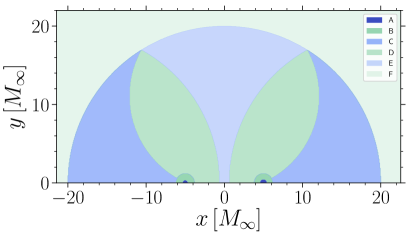
Figure 1: The typical bispherical domain decomposition used in this work. Depicted with different shadings are the various coordinate domains where: regions A are the excised regions of each BH; regions B have a spherical outer radius with an adapted inner radius shared A; regions C, D, and E are the bispherical domains, and region F is the compactified region. Note that this decomposition is rotationally symmetric with respect to the $x$-axis.

The connection between the two components of the binary is done via a set of five domains that implement a bispherical coordinate system. The description is made complete by an additional compactified domain that extends up to spatial infinity by means of the use of a compactified coordinate $1/r$. As a result, the description of a binary system involves a minimum set of twelve domains. An example of this multi-domain setting is shown in Fig. 1 where regions A highlight the excised regions of each BH; regions B have a spherical outer radius with an adapted inner radius shared with region A; regions C, D, and E consist of the bispherical domains (see Ref. Grandclement (2010a) for their details); and region F is the compactified region.

In each domain, the fields are described by their spectral expansion with respect to the numerical coordinates. Chebyshev polynomials are used for variables with no periodicity, such as the radial coordinate, while trigonometrical functions are employed for variables that are periodic, such as the spherical angles of the bispherical coordinates. The choice of the spectral basis, essentially the parity of the functions, can be used to enforce additional conditions, such as regularity on an axis of rotation, or symmetries, like the one with respect to the orbital plane.

Through the spectral representation the residual of the various bulk, boundary, and matching equations is computed. Depending on the operations involved, it is more advantageous to represent the fields either by the coefficients of the spectral expansion or by their values at the collocation points. Once the residuals are known, they are used to find a discrete system by means of a weighted residual method. In the case of the Kadath library, one uses a so-called “tau-method”, which aims at minimising the coefficients of the residuals by expanding the residuals $R$ onto a set of test functions $\xi$ (i.e., the domain basis functions) such that the scalar product $\langle R|\xi\rangle=0$. In the tau method, the equations corresponding to the higher order terms can be replaced in order to enforce boundary and domain matching conditions Grandclément and Novak (2009); Grandclement (2010b). The novel parts of the spectral-solver library introduced in this work refer in particular to the fluid equations needed when solving for neutron stars, as those equations have non-standard properties, such as degeneracies at the surface. Additionally, modifications of the BBH and BNS spaces along with the introduction of a BHNS space and major performance optimisation were essential for this work.

The resulting discretized system is solved by means of a Newton-Raphson iteration. The computation of the Jacobian of the system is done numerically and in parallel thanks to the ability of the code to keep track not only of the value of the fields, but also of their derivative. This is implemented by the use of automatic differentiation (see Sec. 5 of Grandclement (2010a)) and a MPI-parallelised iterative solver.

The equations are, as long as not stated differently, implemented as they are formulated throughout this paper. By using the capabilities of the spectral-solver library, the equations are written in a LaTeX-like format, making changes and generalisations to the system of equations simple and straightforward. Since the solution is known as a spectral expansion of the underlying fields, we generally start generating the solution at very low resolution with largely reduced computational resources needed for the first, coarse solution. Interpolating this solution to a space of higher resolution gives a very good initial guess, so that the Newton-Raphson method generally converges in only a few steps (down to a single one), depending on the previous resolution.

The solvers for the different physical binary systems are coded as stand-alone routines that are linked to the spectral-solver library and used in conjunction with configuration files in order to steer the physical parameters, as well as the different solving stages explained in the next sections III.1–III.3. Additionally, our solvers leverage Kadath’s parallel capabilities, which allows our code to easily scale on high performance computing systems for an efficient calculation of the ID. As a reference, low-resolution ID could be obtained within a couple of hours with $\gtrsim 128$ CPU cores, whereas higher resolution would require $\gtrsim 1000$ and a larger timescale. Noteworthy the solvers scale almost perfectly with increasing number of cores up to $\gtrsim 32000$ cores.

III.1 Binary black-hole (BBH) solver

To obtain BBH ID, we employ an iterative scheme that constructs a BBH system starting from flat-spacetime (i.e., $\alpha=\Psi=1$ and $\beta_{0}^{i}=0$). The system slowly adds constraints over the course of six stages so as to not introduce too many degrees of freedom initially, which could result in the solution diverging prematurely. As noted above, this can be done at very low resolution with only the final step repeated to obtain the desired final resolution.

In the following we describe the different stages and subsets of equations that need to be solved numerically to reach a fully constrained BBH solution.

III.1.1 Pre-conditioning

In the so-called “pre-conditioning stage” , we solve only for Eqs. (8) and (9), while enforcing an initial guess for the fixed radius of the excised region ($R_{\rm BH}={\rm const.}$), for a fixed lapse on the horizon ($\alpha|_{S_{\rm BH}}={\rm const.}$, where $0<\alpha<1$), and a vanishing shift ($\beta_{0}^{i}=0$). This amounts to solving the Laplace equations for $\alpha$ and $\alpha\Psi$, and is used to initialise the scalar fields smoothly over the entire domain decomposition given the inner and outer boundary conditions before introducing terms involving $\beta^{i}$.

III.1.2 Fixed mass and orbital velocity

After the pre-conditioning stage, we solve for the simplest system involving the shift vector field, which is that of an equal mass, corotating BBH system with a fixed orbital frequency, namely that given by a Keplerian estimate obtained using the fixed black-hole masses. Upon inspection of Eq. (53), it is possible to note that in the corotating frame the tangential term will vanish when a black hole is corotating with the binary. Therefore, Eq. (53) reduces to

$$\beta^{i}|_{S_{\rm BH}} =\alpha\Psi^{-2}\tilde{s}^{i}\,.$$

In this stage, we solve Eqs. (9)–(10) while still utilising a fixed value for the lapse at the boundary of both black holes ($\alpha|_{S_{\rm BH}}={\rm const.}$). However, the mass of the black hole is no longer fixed by a constant radius and, instead, the variable radius is solved for by imposing a constant irreducible mass utilising (29).

III.1.3 Corotating binaries

Next, the same system of equations is solved again, but for a fixed equal-mass, corotating system, where the orbital angular frequency $\Omega$ is now fixed by imposing the quasi-equilibrium constraint, i.e., the general-relativistic virial theorem Gourgoulhon and Bonazzola (1994)

$$M_{{}_{\rm ADM}}-M_{{}_{\rm K}}=0\,.$$ (58)

This results in the first fully self-consistent BBH configuration representing a corotating black-hole binary in quasi-circular orbit.

III.1.4 Full system: fixed-lapse boundary conditions

Next, the converged corotating solution is further generalized to arbitrary masses $M_{1,2}$ and dimensionless spins $\chi_{1,2}$ while still utilising a fixed value of the lapse on the horizon. When obtaining such solutions there are a few remarks that are worth making.

First, when changing from an equal-mass binary to an unequal-mass binary, it is important that the total $M_{{}_{\infty,{\rm BBH}}}$ is kept constant; failing to do so, e.g., allowing for differences in $M_{{}_{\infty,{\rm BBH}}}$ as small as $\sim 2\%$, implies that the solution for the shift from the previous stage will deviate too strongly from the final result, thereby causing the overall solution to diverge. Conversely, imposing $M_{{}_{\infty,{\rm BBH}}}={\rm const.}$ allows for changes in the mass $q$ up to a factor of $\sim 4$. Second, using a fixed lapse is essential when solving for a binary for the first time, or when making significant changes to the parameters of a previous solution; failing to do so introduces problems in the subsequent stage of the solver, when von-Neumann boundary conditions are introduced. Finally, large changes in the mass ratio requires incremental solutions and, in some cases, higher resolution to obtain a solution to properly resolve the regions close to the excision boundary.

Note that since, at this stage, the masses are no longer limited to an equal-mass configuration, the “center of mass” of the system is unconstrained and needs to be determined via the condition that the asymptotic net linear momentum of the system is zero, i.e.,

$$P^{i}_{{}_{\rm ADM}}=0\,.$$ (59)

In practice, since our coordinate system is always centered at the origin, the corrections coming from enforcing condition (59) – namely that the helical Killing vector describes a stationary system that is corotating and centered on the center of mass – are added to our helical Killing vector field, which now takes the form

$$\xi^{i}=\Omega\partial_{\phi}^{i}(\bm{x}_{\rm com})\,,$$ (60)

where $\bm{x}_{\rm com}$ represents now the location of the orbital rotation axis, whose origin we define to be the “center of mass” of the system in this context throughout this paper.

III.1.5 Full system: von-Neumann boundary conditions

Finally, the von-Neumann boundary condition is imposed on the excision boundary to relax the necessity to set an arbitrary constant lapse across the horizon Cook and Pfeiffer (2004)

$$D_{\bm{n}}(\alpha\Psi) =0\,,$$ (61)

with $\bm{n}$ being the normal vector field on the excision sphere. However, because this boundary condition introduces a considerable sensitivity to changes in the solution, it is employed only as the final step of the convergence sequence.

III.1.6 Eccentricity Reduction

Strictly speaking the reduction of the eccentricity is not part of the procedure for finding self-consistent initial data of binary systems, which completes with the step in Sec. III.1.5. Such initial data, however, although being an accurate solution of the constraint equations, normally leads to orbital motion that is characterised by a nonzero degree of eccentricity. The amount of eccentricity depends sensitively on the properties of the system (mass ratio and spin) and is most often due to the various assumptions that are tied with the calculation of the initial data, e.g., quasi-circularity, conformal flatness, etc.

Independently of its origin, such eccentricity represents a nuisance that needs to be removed as binaries of stellar-mass compact objects are expected to be quasi-circular in the last stages of the inspiral. In essence, eccentricity is reduced by utilising input values of $\Omega$ and $\dot{a}$ as constants when solving for the new ID. Since $\Omega$ is fixed, Eq. (58) is neglected in the system of equations to be solved. Estimates for $\Omega$ and $\dot{a}$ can either be those derived from approximate treatments, such as post-Newtonian theory [see, e.g., (75) and (74) in Appendix B] or from an iterative eccentricity reduction procedure. In this second approach, corrections to $\Omega$ and $\dot{a}$ are calculated by using the ID in short evolutions and by fitting the orbit using Eqs. (68)-(72) to obtain the corrections $\delta\dot{a}$ and $\delta\Omega$ to the previous estimates Pfeiffer et al. (2007); Husa et al. (2008). The subtleties of this trial-and-error approach are discussed in detail in Appendix A and the included references.

III.2 Binary neutron-star solver

When compared to a BBH system, the BNS solver is much less sensitive to the initial conditions and, therefore, there is no need for additional sub-stages in the solution process. This is partly due to the fact that the iterative scheme is started already with a reasonable initial guess by importing and combining the solutions for static and isolated stars, (i.e., the Tolmann-Oppenheimer-Volkov or TOV equations), but also because the inner boundary conditions on the excision spheres are susceptible to small changes in the case of a BBH. In addition, the gravitational fields and their derivatives are overall smaller and thus the nonlinearities in the equations less severe.

The scalar fields for the lapse $\alpha_{\text{NS}}$ and conformal factor $\Psi_{\text{NS}}$ from the TOV solutions are interpolated onto the BNS domains using a simple product of the two independent solutions at a given Cartesian coordinate $\bm{x}$

$$\alpha_{{}_{\rm BNS}}(\bm{x}) =\alpha_{{}_{\rm NS1}}(\bm{x}-\bm{x}_{c1})\alpha_{{}_{\rm NS2}}(\bm{x}-\bm{x}_{c2})\,,$$ (62)

$$\Psi_{{}_{\rm BNS}}(\bm{x}) =\Psi_{{}_{\rm NS1}}(\bm{x}-\bm{x}_{c1})\Psi_{{}_{\rm NS2}}(\bm{x}-\bm{x}_{c2})\,,$$ (63)

where $\bm{x}-\bm{x}_{c}$ represents the coordinate system with origin in the center of the given compact object. Additionally, the matter is imported into the stellar interior domains and set to zero in all domains outside of the neutron stars. Given the surface of the stars are described by adapted spherical domains, the mapping of the adapted domains must also be updated based on the mappings from the isolated TOV solutions. Finally, the shift is discarded as the solver is more reliable when starting from zero shift.

As described in Sec. II.5, also in the case of a BNS system we are solving Eqs. (8)–(10) scaled by the ratio $p/\rho$, together with Eqs. (52) and (47), with the additional constraints of $\phi|_{x_{c}}=0$ and a fixed $M_{b}$ defined by Eq. (33).

III.2.1 Full System

To close the system of equations, there is still the need of a condition to constrain the orbital frequency, $\Omega$, and, in general, the “center of mass”, $\bm{x}_{\rm com}$. Additionally, the neutron stars – contrary to a black hole – have an anisotropic radius distribution along their adapted surface such that the matter distributions is not constrained to remain at a fixed distance with respect to the origin of the innermost domains. To break this degeneracy, we add two conditions for the two unknowns in terms of the derivative of the enthalpy

$$D_{x}H|_{x_{c_{1,2}}} =0\,,$$ (64)

where $x$ is the coordinate direction along which the two stellar centres are placed and $x_{c_{1,2}}$ are the positions of the fixed centres of the stars along the $x$-axis. Equations (64) are the so-called “force-balance equations” Gourgoulhon et al. (2001) and complete the system needed to obtain the ID in quasi-equilibrium.

III.2.2 Reduced system: fixed linear Momentum

In case of high mass ratios, the full system as implemented in stage III.2.1, together with Eq. (64), yields binary systems with a non-negligible amount of total linear momentum $P^{i}_{{}_{\rm ADM}}$ at infinity. In turn, this leads to an undesirable spurious drift of the center of mass of the system during its evolution. In the same context, we observed that solving Eq. (64) separately for each star produces inconsistent orbital frequencies when considering two stars that differ significantly in spin and in mass. Since adding an extra constraint to fix the total linear momentum renders the system over-determined, and a simple averaging of the two separate solutions for $\Omega$ Dietrich et al. (2015); Tichy et al. (2019) is incompatible for the more challenging configurations involving a high mass ratio combined with extreme rotation states, we follow a different route.

In particular, we take the matter distribution and the orbital frequency $\Omega$ computed from the previous stage and define both to be constant, making Eq. (64) redundant. At this point, we can use the condition

$$P^{i}_{{}_{\rm ADM}} =0\,,$$ (65)

to determine a correction to the location of the axis of rotation of the spatial part of the Killing vector $\xi^{i}$, just as for a BBH configuration.

Doing so necessarily leads to slight differences in the velocity field of the neutron stars due to changes in the velocity potential, which incorporates and adapts to the different velocity contributions. Most importantly, doing so introduces small deviations in $M_{b}$ through the Lorentz factor $W$ present in the integral (33). Since the rest-mass is a fundamental property of the binary from and is conserved throughout the evolution by (42), it is important to enforce that the desired value is specified with precision. We accomplish this by a simple rescaling of the form

$$H\to H =H_{\rm const.}(1+\Delta_{H})\,,$$ (66)

where $H_{\rm const.}$ is the fixed matter distribution from the previous stage and $\Delta_{H}$ is the (small) correction needed to enforce that the baryon mass is the one expressed by Eq. (33).

Ultimately, the first integral Eq. (52) is the only equation that is violated by the rescaling discussed above, although only to a limited extent. While this violation certainly has an impact on the equilibrium of the two stars, this impact is overall negligible. Indeed, numerical-evolution tests spanning throughout the allowed parameter space in terms of mass ratio and spin has shown that the perturbations of the stars are increased insignificantly when compared to the fully self-consistent solutions resulting from stage III.2.1. Furthermore, these perturbations are a priori indistinguishable from those introduced in the binary simply because of the approximate nature of the condition Eq. (52) in the case of high spins. More importantly, numerical evolution of high spin and mass ratio systems without explicitly fixing (65) by using only III.2.1 exhibit the same orbital evolution as the fixed systems, apart from a strong center of mass drift. Thus, the prescription above allows us to have a precise control of the drift of the center of mass and of the baryon mass of the binary.

III.2.3 Eccentricity Reduction

As in the BBH case, in order to reach a solution with reduced orbital eccentricity, the quantities $\Omega$ and $\dot{a}$ need to be fixed via an iterative procedure fitting the trajectories in terms of Eqs. (71) and (72) so as to obtain the intended corrections. Since in this case $\Omega$ has to be fixed, we follow the same approach as in stage III.2.2 and rescale the matter of the original solution from the stage III.2.1. In this way, employing Eq. (65), the ID features both a reduced orbital eccentricity and a very small center-of-mass drift.

III.3 Black-hole neutron-star solver

Finally, to show the flexibility in applying the extended Kadath spectral-solver library, we can use much of the infrastructure presented above for BBHs (section III.1) and BNSs (section III.2) to construct binaries composed of a black hole and a neutron star.

For the initial guess, we currently start with an irrotational, equal-mass system utilising a previously solved BNS ID and an isolated black-hole solution. This provides a very good estimate for $\alpha$ and $\Psi$, as well as for the matter-related quantities $\phi$ and $H$. The shift vector, however, is discarded as this can have a negative impact on the initial convergence. We note that, in principle, it is also possible to start directly from a static TOV and single black-hole initial guess for the spacetime. During the import, spherical shell domains are added outside of the black hole to obtain the same resolution near the excision boundary as that which is near the surface of the neutron star. These additional shells can be removed or added as necessary to obtain the desired resolution.

III.3.1 Initial system: fixed-lapse boundary condition

By combining the two converged datasets, we start our two-stage solver starting with an initial equal-mass and irrotational BHNS system. More specifically, in the first stage we solve the neutron-star part using the same system of equations for the matter component described in Sec. III.2.1. On the other hand, when considering the black-hole component, we utilise the system of equations described Sec. in III.1.4, which fixes the lapse function on the horizon based on the imported isolated black-hole solution. This stage proved necessary as the von-Neumann boundary condition was excessively sensitive and would otherwise result in a diverging solution.

The orbital frequency $\Omega$ of the binary is set solely by Eq. (64), but, unlike for a BNS system where Eq. (64) consists of two distinct equations, we still fix the center of mass by imposing $P^{i}_{{}_{\rm ADM}}=0$ without over-determining the system of equations.

III.3.2 Full system: von-Neumann boundary condition

In this second stage, we repeat the steps just described above, but exchange the constant lapse constraint on the horizon with the von-Neumann boundary condition as described in Sec. III.1.5. Once a first configuration has converged in this stage, all further modifications, such as iterative changes to the spins and the mass ratio, can be made while subsequently resorting only to this final stage.

III.3.3 Eccentricity Reduction

As in the BBH and BNS scenarios, $\Omega$ and $\dot{a}$ are corrected to remove the spurious eccentricity by using the same iterative procedures already mentioned in Secs. III.1.6 and III.2.3. Additionally, the matter is rescaled as discussed in sections III.2.3 and III.2.2 since $\Omega$ is again a fixed quantity at this stage. Finally, we explicitly enforce Eq. (65) to minimised the residual drifts of the center of mass.

IV Results

In the following, we present a collection of ID configurations generated using the procedures described in Sec. III. Such ID is then employed to carry out evolutions of the various binary systems making use of the general-relativistic magnetohydrodynamics code FIL Most et al. (2019a, b), which is derived from the IllinoisGRMHD code (Etienne et al., 2015), but implements high-order (fourth) conservative finite-difference methods (Del Zanna et al., 2007) and can handle temperature and electron-fraction dependent equations of state (EOSs). Neutrino cooling and weak interactions are included in the form of a neutrino leakage scheme (Ruffert et al., 1996; Rosswog and Liebendörfer, 2003; Galeazzi et al., 2013).

FIL makes use of the Einstein Toolkit infrastructure Loeffler et al. (2012). This includes the use of the fixed-mesh box-in-box refinement driver Carpet Schnetter et al. (2004), the apparent horizon finder AHFinderDirect Thornburg (2004) together with QuasiLocalMeasures Schnetter et al. (2006) to measure quasi-local horizon quantities of the black holes. The spacetime evolution is done either by McLachlan Brown et al. (2009); mcl for the BSSNOK formulation Baumgarte and Shapiro (1999); Shibata and Nakamura (1995) or by Antelope Most et al. (2019a) implementing the BSSNOK Baumgarte and Shapiro (1999); Shibata and Nakamura (1995), Z4c Bernuzzi and Hilditch (2010), and CCZ4 Alic et al. (2012, 2013) formulations.

IV.1 Sequences of compact binaries

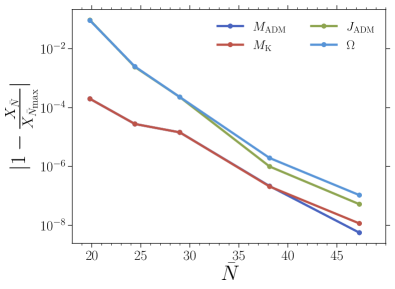
Figure 2: Spectral convergence of the asymptotic quantities described in Sec. II.3 and of the orbital frequency $\Omega$ for an equal-mass BBH system. Shown are the absolute values of the variations of the quantity $X$ at a given effective resolution $\bar{N}$ given by Eq. (67) with respect to the corresponding quantity at the largest effective resolution $\bar{N}_{\rm max}=52$. Clearly the variations decrease exponentially for all quantities considered.

As a first result, and as an effective way to quantify the reliability of our implementations, we perform an initial resolution study to determine if the global properties of the solutions show the expected spectral (i.e., exponential) convergence for increasing number of collocation points. To do so we utilise the asymptotic quantities $M_{{}_{\rm ADM}}$, $M_{{}_{\rm K}}$, $J_{{}_{\rm ADM}}$ defined in Sec. II.3 and the orbital angular velocity $\Omega$ of an equal-mass BBH system. In this context, we define an effective resolution across the whole space following Tacik et al. (2015)

$$\bar{N} :=\left(\sum_{i\in\mathcal{D}}N_{\left(i\right)}\right)^{\frac{1}{3}}\,,$$ (67)

where $N_{\left(i\right)}$ is the total number of points of the $i$-th domain part of the space decomposition $\mathcal{D}$, which is rounded to the closest integer number. In Fig. 2 we report for each quantity $X$ (i.e., $M_{{}_{\rm ADM}},M_{{}_{\rm K}},J_{{}_{\rm ADM}}$, and $\Omega$), the absolute value of the variations of $X$ at a given $\bar{N}$ with respect to the corresponding quantity at the largest value $\bar{N}_{\rm max}$ (i.e., the high-resolution solution). While $M_{{}_{\rm ADM}}$ and $M_{{}_{\rm K}}$ have consistently smaller relative deviations than $J_{{}_{\rm ADM}}$, and $\Omega$, all quantities clearly exhibit the expected spectral convergence.

Next, we present quasi-equilibrium sequences of irrotational BBHs, BNSs, and BHNSs, and compare the corresponding binding energies and orbital angular velocities with the values obtained from fourth-order post-Newtonian (4PN) expressions, namely, Eqs. (77) and (78) (see, Appendix B and (Blanchet, 2014) for a review).

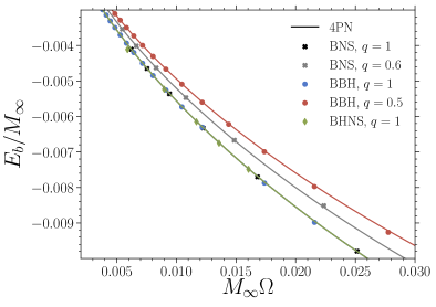
Figure 3: Behaviour of the binding energy [cf. Eq. (24)] as a function of the dimensionless orbital frequency for sequences of irrotational BBH, BNS, and BHNS binaries (coloured filled circles), when compared with the combined with the corresponding 4PN prediction given by Eq. (78) (coloured solid lines). For binaries having the same components, we have considered both equal-mass binaries ($q=1$) and unequal-mass binaries ($q=0.5$ for BBHs and $q=0.6$ for BNSs). Finally, in the case of the BHNS binaries, we have computed a rather extreme equal-mass configurations.

Figure 3, in particular, presents a comparison of the binding energy $E_{b}$ [cf. Eq. eq. 24] of various irrotational compact binaries, namely, BNS (crosses), BBH (filled circles), and BHNS (diamonds), that have either equal masses ($q=1$) or unequal masses ($q=0.5,0.6$). In the case of binaries with at least one neutron star, we model the latter by a single polytrope with $K=100$ and $\Gamma=2$ as a function of the dimensionless orbital frequency $M_{\infty}\Omega$. Note that both for equal-mass and unequal-mass binaries our numerical solutions closely follow the analytical 4PN estimates (solid lines).

Following a similar spirit, Fig. 4 reports the binding energy as a function of the normalised orbital frequency for a selection of equal-mass, irrotational or spinning BNS configurations with spins that are either aligned and anti-aligned to the orbital angular momentum. The EOS used is the same as in Fig. 3 (a single polytrope with $K=100$ and $\Gamma=2$). As can be clearly seen, binaries with spin that are aligned with respect to the orbital angular momentum are less bound than the irrotational counterparts, which, in turn, are less bound than the binaries with anti-aligned spins. This result, which is embodied already in the PN equations (see solid lines), confirms what has been presented in Refs. Dietrich et al. (2015); Tichy et al. (2019) and highlights that binary systems with significant aligned spins will require a larger number of orbits before merging.

IV.2 Evolutions of black-hole binaries

In the following we present the results of the evolutions of BBHs whose ID have been produced with our new spectral solver. Note that our evolutions, although comprehensive of all the relevant cases, do not explore any new aspect of the dynamics of compact binaries that has not been presented already in the literature. Rather, here they are meant to be used mostly as representative test cases and clear proofs of the considerable capabilities of the new spectral-solver library.

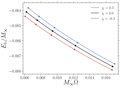
Figure 4: Same as in Fig. 3 but for equal-mass, BNS configurations that are either irrotational ($\chi=0$) or spinning ($\chi=\pm 0.3$), with spins aligned to the orbital angular momentum. Also in this case, the coloured solid lines refer to the 4PN predictions (78), which provide an accurate estimate even in the presence of high spins in the range of the given orbital frequencies.

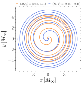
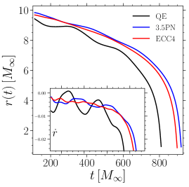
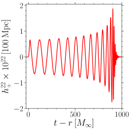
Figure 5: Left: Orbital trajectories of a representative BBH configuration reproducing the properties of the GW150914 event; shown with the light-orange track is the orbit of the primary black hole, while the light-blue track refers to the secondary. Middle: Evolution of the coordinate separation $r(t)$ of the GW150914 ID when considering only the quasi-equilibrium assumption (black solid line), the 3.5PN estimates for $\dot{a}$ and $\Omega$ (blue solid line), or after the fourth iteration (ECC4) of the eccentricity-reduction procedure (red solid line). The inset shows the time derivative of the coordinate separation, $\dot{r}(t)$, for the same datasets. Right: gravitational-wave strain of the $\ell=m=2$ multipole of the $+$ polarization for the ECC4 dataset.

IV.2.1 Representative mass ratio and mixed spins

As a realistic test case to exercise the capabilities of the BBH ID solver, we generate ID based on the GW150914 detection and thus assuming that the mass ratio is $q=0.8055$. The primary black hole is set to have a dimensionless spin of $\chi_{1}=0.31$ and the secondary $\chi_{2}=-0.46$, while we fix the initial separation to $d_{0}=10\,M$; this setup is very similar to the one used in Ref. Wardell et al. (2016). A summary of the dynamics of this binary is offered in Fig. 5, whose different panels report, respectively, the orbital tracks (left panel), the coordinate separation between the two black holes at different stages of the eccentricity-reduction (middle panel), and the corresponding gravitational-wave strain in the $\ell=m=2$ multipole of the $+$ polarization (right panel). Note that the left and right panels refer to the configuration with the smallest eccentricity.

The spins of both black holes are perpendicular to the orbital plane and, as a first step, we generate a corresponding dataset under the assumption of quasi-equilibrium (QE) using Eq. (58). As expected from this raw ID, the actual evolutions reveal that the initial orbital eccentricity is large, as can be can be seen from the black line in the middle panel of Fig. 5; in the same panel, the inset provides a measure of the time derivative of the coordinate separation $\dot{r}(t)$. Fortunately, this problem can be resolved rather straightforwardly and already by simply utilising the 3.5PN estimates for the expansion coefficient, $\dot{a}$ [i.e., Eq. (74)], and for the orbital frequency, $\Omega$ [i.e., Eq. (75)]. As shown with the blue line in the middle panel of Fig. 5, this simple estimate already results in a greatly reduced orbital eccentricity.

An additional reduction can be obtained after performing four iterations of the eccentricity-reduction procedure described in Sec. III.1.6 and Appendix A, where we start from the 3.5PN ID until we obtain an orbital eccentricity of the order of $10^{-4}$; we refer to this ID as “ECC4” hereafter. More specifically, for each iteration of the eccentricity-reduction procedure, the eccentricity is measured using the coordinate separation between the centres of both horizons $r(t)$, and its time derivative $\dot{r}(t)$; the two quantities are then fitted using the ansatzes (68) and (69). We note that both quantities are measured during the first three orbital periods to ensure a consistent measurement of the eccentricity, which, in turn, allow us to obtain accurate corrections to the quantities $\Omega$ and $\dot{a}$ [cf. Eqs. (71) and (72)]. Experience has shown that relying on a single orbit does not yield sufficiently accurate estimates for corrections to $\Omega$ and $\dot{a}$, thus not yielding a significant decrease in the eccentricity. In all cases, we are able to obtain consistent measurements and corrections from $r(t)$ and $\dot{r}(t)$ up to an eccentricity $\lesssim 10^{-3}$. For eccentricities smaller than these and up to an eccentricity $\lesssim 10^{-4}$, we obtain more reliable results using only the parameters fitted from $\dot{r}(t)$, since the fitting parameters for $r(t)$ are unreliable due to the eccentricity having a weak impact on the separation distance – the oscillations are too small to fit – when using the ansatz (68). Indeed, as remarked also by other authors Pfeiffer et al. (2007); Husa et al. (2008); Buonanno et al. (2011); Kyutoku et al. (2014), when considering orbits with eccentricities $\lesssim 10^{-3}$, the correction parameters are very sensitive to the fitting procedure used, to the initial estimates for these parameters, and to the evolution window being analysed.

IV.2.2 Impact of the ID resolution on the gravitational-wave phase

To further quantify the impact of the resolution with which the ID is computed on the overall error budget as seen from an evolution perspective, we run a series of nine simulations utilising the ECC4 initial dataset to determine the convergence of the gravitational phase evolution up to merger. The latter is a good choice being a coordinate independent quantity and the most important in waveform modelling for template matching Hinder and et al. (2013).

This series of nine evolutions consists of a binary constructed with three different ID resolutions, i.e., $\bar{N}=24,38$, and $42$, and evolved with three different evolution resolutions, i.e., $\Delta x_{\rm{LR}}/M=0.024$, $\Delta x_{\rm{MR}}/M=0.019$, and $\Delta x_{\rm{HR}}/M=0.015$. The latter correspond to a number of points across the apparent horizon (AH) of about $n_{\rm{AH}}=35$, $n_{\rm{AH}}=45$ and $n_{\rm{AH}}=55$ respectively. For all cases considered, the spacetime evolution utilises an 8th-order finite-differencing scheme so as to minimise the error in the evolution of the binaries.

	$\left|\Delta\varphi\right|_{{}_{\rm LR}}$	$\left|\Delta\varphi\right|_{{}_{\rm MR}}$	$\left|\Delta\varphi\right|_{{}_{\rm HR}}$	$M_{{}_{\rm ADM}}$ $\left[{M}\right]$	$J_{{}_{\rm ADM}}$ $\left[{M}^{2}\right]$
$\bar{N}=24$	$12.214$	$1.888$	$0.095$	$0.9897$	$0.9572$
$\bar{N}=38$	$12.067$	$1.771$	$0.008$	$0.9899$	$0.9573$
$\bar{N}=42$	$12.067$	$1.770$	$0.000$	$0.9899$	$0.9573$

Table 1: Gravitational-wave phase differences for the $\ell=m=2$ strain mode of the $+$ polarisation as computed at merger when employing either different ID resolutions ($\bar{N}=24,38,42$) or evolution resolutions (LR, MR, HR). Also reported are the corresponding values of the ADM mass $M_{{}_{\rm ADM}}$ and ADM angular momentum $J_{{}_{\rm ADM}}$ as computed from the ID.

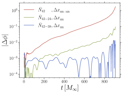
Figure 6: Evolution of the differences in the gravitational-wave phase computed from the $\ell=m=2$ multipole of the $+$ polarization produced by BBH configurations representative of the GW150914 event. Different lines contrast the difference when considering either different effective ID resolutions, i.e., $\bar{N}=24,38,42$), or different evolution resolutions, i.e., low resolution ($\Delta x_{\rm{LR}}$), medium resolution ($\Delta x_{\rm{MR}}$), and high resolution ($\Delta x_{\rm{HR}}$). Note that the contribution of the ID to the final error budget is always subdominant at the evolution resolutions employed here.

In Tab. 1 we report the magnitude of the phase differences at merger of the phases of the $\ell=m=2$ mode gravitational-wave strain. For each of the cases reported, $|\Delta\phi|$ is computed as the difference between the gravitational-wave phase at merger from evolutions at a given resolution (i.e., LR, MR, HR) from ID computed with a given set of collocation points (i.e., $\bar{N}=24,38,42$) relative to the highest-resolution setup (i.e., HR, $\bar{N}=42$). In addition, and as a reference, Tab. 1 reports the various ADM quantities for each ID resolution.

Similarly, but only for a subset of three binaries in Tab. 1, we show in Fig. 6 the full time evolution of the phase differences. In particular, we concentrate on evolutions capturing the differences of the ID datasets with $\bar{N}\in\left\{24,38\right\}$ and evolved at the highest resolution HR. These differences are indicated with blue and green lines in Fig. 6 and are meant to highlight the actual impact of the ID resolution on the error budget of the simulation. In addition, we report with a dark-red line the phase difference that develops when comparing evolutions with ID computed at the highest resolution (i.e., $\bar{N}=42$) between the medium (MR) and high-resolution (HR) setups. By contrast, this line is meant to highlight the actual impact of the evolution resolution on the error budget.

As can be seen already from Fig. 6 and fully deduced from Tab. 1, the total phase error at merger is completely dominated by the evolution resolution, at least for the resolutions considered here. There is only a very weak dependence on the ID resolution, which converges away rapidly with increasing number of collocation points. Stated differently, the ID error contribution is subdominant already with $\bar{N}=24$ and becomes even less relevant as the number of collocation points is increased. As customary in these evolutions, the phase difference increases as the merger is approached and evolution becomes increasingly nonlinear. However, even in the case of the low-$\bar{N}$ ID, the phase difference is always below $\Delta\phi\sim 0.1\,\rm{rad}$. In contrast, the phase difference between the two highest evolution resolutions is one magnitude larger, $\Delta\phi\sim 1.0\,\rm{rad}$, and is dominating over the whole inspiral. These results clearly indicate that for vacuum solutions at the resolutions considered here – and for the ranges of mass ratios and spins explored so far – the ID resolution plays only a minor role for the total phase error budget and rather low resolutions can be used as long as the orbital frequency is fixed by PN estimates or iterative eccentricity reduction.

IV.3 Evolutions of neutron-star binaries

We next present the results of the evolutions of BNS configurations whose quasi-equilibrium initial configurations have been produced with the new solver utilising the Kadath library. Also in this case, our evolutions are here meant to be used mostly as representative test cases and clear proofs of the capabilities of the new spectral-solver library to produce astrophysically useful data, rather than providing new insight into this process.

Reference	$\omega$	$M_{b}$	$M_{{}_{\rm QL}}$	$\mathcal{S}_{{}_{\rm QL}}$	$\mathcal{S}_{{}_{\rm QL}}/M^{2}$
	$[M^{-1}_{\odot}]$	$[M_{\odot}]$	$[M_{\odot}]$	$[M^{2}_{\odot}]$
Tichy+ 2019 Tichy et al. (2019)	$0.00000$	$1.7745$	$1.620$	$-0.0007$	$-0.0003$
this work	$0.00000$	$1.7745$	$1.620$	$-0.0007$	$-0.0003$
Tichy+ 2019 Tichy et al. (2019)	$0.01525$	$1.7745$	$1.626$	$\phantom{-}0.8652$	$\phantom{-}0.3217$
this work	$0.01525$	$1.7745$	$1.626$	$\phantom{-}0.8631$	$\phantom{-}0.3209$

Table 2: Comparison with the properties reported in Ref. Tichy et al. (2019) for either an equal-mass irrotational, or equal-mass spinning BNS configuration using a single polytrope with $K=123.6$ and $\Gamma=2$. Listed are the quantities that can be compared directly: the fixed spin frequency parameter, $\omega$, the fixed baryonic mass, $M_{b}$, the quasi-local ADM mass, $M_{{}_{\rm QL}}$, the spin angular momentum, $\mathcal{S}_{{}_{\rm QL}}$, and the dimensionless spin normalized by $M=1.64\,M_{\odot}$. The agreement is very good and the small differences in the quasi-local measurements are mostly due to the different approaches to perform the measurements.

IV.3.1 Spinning binary neutron stars: a comparison

As a first general test of a BNS system containing spinning companions, we consider the equal-mass, equal-spin BNS model first presented in Ref. Tichy et al. (2019), which is based on a single polytrope with $K=123.6$ and $\Gamma=2$. A similar stellar model was considered also in Ref. Tacik et al. (2015), but unfortunately no updated model was discussed in the subsequent work Ref. Tacik et al. (2016). For this binary, the spin parameter is fixed to $\omega=0.1525$ [cf. Eq. (49)], together with a baryonic mass of $M_{b}=1.7745\,M_{\odot}$, and a coordinate separation of $d=47.2\,M_{\odot}$.

Table 2 offers a comparison of the quasi-local measurements for the mass and spin computed here with the corresponding quantities reported in Ref. Tichy et al. (2019). Note that while there is an excellent agreement in the quasi-local mass computed by (34), there is a small deviation in the quasi-local spin. We believe this difference is due to the method used in Ref. Tichy et al. (2019) to compute the spin, which differs from the one employed here and that follows the one in Ref. Tacik et al. (2015); the differences are however minute and smaller than $0.3\%$.

To further assess the correctness of the implementation of the spin-velocity field given by Eq. (48) and the resulting spin angular momenta, we created a sequence of equal-mass BNS models based on a single polytrope with $K=123.6$ and $\Gamma=2$. The sequences are parameterized by the increasing spin parameter $\omega$ for a fixed mass $M_{{}_{\rm ADM}}=1.64\,M_{\odot}$, thus matching the models given in Tacik et al. (2015, 2016); Tichy et al. (2019). Note that the baryonic mass decreases for increasing spin at fixed $M_{{}_{\rm ADM}}$ due to the growing contribution of the spin angular momentum to the gravitational mass and, thus, has to be adjusted by matching it to single-star models with the same $M_{{}_{\rm ADM}}$ and $\chi$.

The resulting dependency between the spin parameter $\omega$ and dimensionless spin $\chi$ is shown in Fig. 7 and combined with a smoothly interpolated representation of the data given in Ref. Tacik et al. (2015, 2016); Tichy et al. (2019); we note that the results reported in Ref. Tacik et al. (2015) (black dashed line in Fig. 7) were generated with an incorrect first-integral equation and has been corrected in Ref. Tacik et al. (2016) (blue solid line). It is evident from Fig. 7 that all three codes reproduce the same relation at low spin angular momenta and that this is almost linear. However, for larger spin angular momenta the relation becomes nonlinear with the spins increasing rapidly as function of the frequency parameter. Note that for very high spins a difference appears between the values computed here and those reported in Ref. Tichy et al. (2019) (dark-red solid line). As discussed above, we believe this discrepancy originates from different methods employed to compute the quasi-local spin angular momentum; furthermore, since this quantity is defined only approximately, the variations measured are not a source of concern.

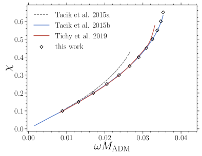
Figure 7: Dimensionless spin $\chi$ as function of the stellar spin frequency parameter $\omega$ for a sequence of BNS configurations using a single polytrope with $K=123.6$ and $\Gamma=2$. The numerical data (open symbols) is compared with the interpolating functions reported in Refs. Tacik et al. (2015, 2016); Tichy et al. (2019), indicating the very good agreement.

IV.3.2 Eccentricity reduction with unequal masses and spins

As done for BBHs, we also employ an iterative eccentricity-reduction procedure on our BNS ID that follows the same logic mentioned above and presented in more detail in Appendix A. As it is natural to expect, BNSs that are increasingly asymmetric in mass and spin exhibit an increase in the initial eccentricity starting from the quasi-equilibrium solution using the force-balance constraint equation (64). Especially in binaries with components with large dimensionless spin, i.e., $\chi\gtrsim 0.6$, the initial eccentricity can be extremely large and becoming larger with increasing spins and decreasing mass ratios.

As a general example of our eccentricity-reduction process involving extreme spins, we generate a BNS configuration using the beta-equilibrium slice of the finite-temperature TNTYST EOS Togashi et al. (2017) with $M_{\infty}=2.7\,M_{\odot}$, $q=0.6875$, $\chi_{1}=0$, and $\chi_{2}=0.6$, where the highly spinning star is also the more massive one.

Starting from the quasi-equilibrium solution, the eccentricity of the orbit is progressively reduced via a total of four steps in which we use the fitting ansatz (69) for the time derivative of the proper separation of both neutron stars. We remark that we employ a Newtonian estimate for the barycentre of both stars to circumvent the high-frequency noise in the location of the stellar centres that appears when defining the stellar centres by a maximum density measurement alone. The eccentricity reduction is performed using a lower resolution ID with $\bar{N}=29$ and a medium evolution resolution of $\Delta x=0.2\,M_{\odot}\,\approx 295\,\rm{m}$. For the construction of the fourth and final eccentricity-reduced dataset, the resolution is increased to $\bar{N}=38$. We note that further increasing/decreasing the resolution of the ID between these two values of $\bar{N}=29,38$ at this stage of the procedure has no substantial effect on the resulting evolution, as we further discuss below (see Sec. IV.3.3).

In Fig. 8 we present the evolution of the proper separation of the initial (black solid line) and final (red solid line) datasets in the eccentricity reduction procedure. In addition, the same system is solved using fixed values of $\Omega$ and $\dot{a}$ estimated from the 3.5PN expression given by Eqs. (74) and (75) (blue solid line), which already provide a considerable reduction of the eccentricity. With the final set of parameters we arrive at a residual eccentricity $\lesssim 10^{-4}$, at which point the mentioned fitting procedure is no longer reliable and further reduction becomes infeasible.

Figure 8 shows that the eccentricity-reduction procedure performs very well even when starting with binary configurations where the high spin of the more massive companion leads to very large initial eccentricities. At the same time, it is also apparent that multiple iterations of the reduction can be skipped by simply starting from the 3.5PN – or higher-order PN estimates – of the initial orbital parameters. We thus recommend to apply these estimates in any case instead of resorting to solutions based on the plain force-balance equation (64) even when no further iterative reduction is conducted. Indeed with very high spins as in this binary, resorting to the 3.5PN expressions leads to eccentricities that are of the same order as those encountered in standard irrotational quasi-equilibrium configurations without eccentricity reduction.

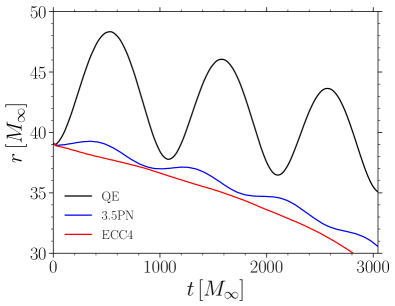
Figure 8: Representative example of the iterative eccentricity reduction for a rapidly spinning BNS system modelled with the TNTYST and with $M_{\infty}=2.7$, $q=0.6875$, $\chi_{1}=0$ and $\chi_{2}=0.6$. Shown is the evolution of the proper separation between the two stars when using only the quasi-equilibrium ID (black line; QE), or when utilising the 3.5PN estimates for $\Omega$ and $\dot{a}$ (blue line; 3.5PN), or when employing the ID from the final step of the eccentricity-reduction procedure (red line; ECC4). Note that the QE condition leads to enormous eccentricities for such a highly spinning binary.

IV.3.3 Impact of the ID resolution on the gravitational-wave phase

In analogy with the results presented in Sec. IV.2.1, we next investigate the impact of the ID resolution and of the evolution resolution using the gravitational-wave phase as our reference quantity. For this purpose, we conduct a series of simulations at varying evolution resolutions, namely $\Delta x_{{}_{\rm LR}}=0.25\,M_{\odot}\approx 369\,{\rm m}$, $\Delta x_{{}_{\rm MR}}=0.2\,M_{\odot}\approx 295\,{\rm m}$ and $\Delta x_{{}_{\rm HR}}=0.145\,M_{\odot}\approx 215\,{\rm m}$, in conjunction with three ID resolutions $\bar{N}_{{}_{\rm ILR}}=29$, $\bar{N}_{{}_{\rm IMR}}=38$ and $\bar{N}_{{}_{\rm IHR}}=47$. In particular, we concentrate on five combinations of these resolutions, considering first the two lower ID resolutions ILR and IMR and using them for the HR evolution resolution. Next, we compare and contrast the results to the highest resolution ID IHR, using it to perform evolutions at the three different evolution resolutions LR, MR and HR. As for the binary model, we resort to an equal-mass binary with individual baryonic masses $M_{b}=1.4946\,M_{\odot}$ at an initial coordinate separation of $52.42\,{\rm km}$ using a tabulated version of the SLy EOS Douchin and Haensel (2000).

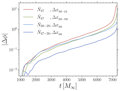
Figure 9: Same as in Fig. 6, but for an equal-mass irrotational BNS system modelled using the SLy EOS. Also in this case, the differences are computed either for different effective ID resolutions ($\bar{N}=29,38,47$) or for different evolution resolutions (LR, MR, HR). Also in this case, the resolution evolution provides the largest contribution to the error budget at least for the resolutions considered here, although increasing the ID resolution can reduce the phase difference for HR evolutions.

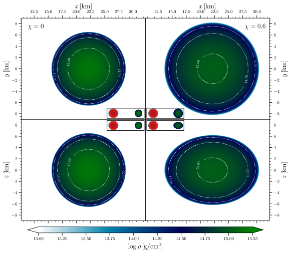
Figure 10: Two-dimensional cuts through the $(x,y)$ (top row) and $(x,z)$ planes (bottom row) of two extreme BNS systems modelled with the TNTYST EOS and having a very small mass ratio ($q=0.455$ corresponding to $M_{1}=2.2\,M_{\odot},M_{2}=1.0\,M_{\odot}$). The left column refers to an irrotational binary ($\chi_{1}=0,\chi_{2}=0$), while the right one to a very large spin asymmetry ($\chi_{1}=0.6,\chi_{2}=0$); the latter is the most extreme BNS configuration considered here. The panels concentrate on the more massive component, but the insets offer views of the whole binaries, where the secondary is marked in red.

We note that in order to remove effects of varying eccentricity at different resolutions introduced by slightly changing orbital parameters – most notably, $\Omega$ – we enforce a well controlled setup with $\Omega$ and $\dot{a}$ fixed by Eqs. (75) and (74), respectively. An alternative route would be to perform a full eccentricity reduction of the orbit to fix both parameters.

As discussed in Sec. IV.2.2, for each simulation we compute the phase evolution of the $\ell=m=2$ mode gravitational-wave strain and present in Fig. 9 the resulting phase errors. We note that – in contrast with what is done for BBHs, where this was not necessary – we exclude the initial phase of the evolution, as the binaries settle down after the junk is radiated away and we align the waveforms at $1000\,M_{\odot}$. When considering the variations in the phase evolution reported in Fig. 9, a few considerations can be made. First, the largest differences in $\Delta\phi$ are measured when considering differences in the evolution resolution (dark-red and green solid lines), with the difference when considering the HR and LR resolutions (dark-red solid line),being larger than when considering the HR and MR resolutions (green solid line). In other words, and as already commented above, the resolution evolution provides the largest contribution to the error budget and having large ID resolution does not provide a more accurate phase evolution for the evolution resolutions considered here. Second, the smallest values of $\Delta\phi$ are obtained when considering the highest evolution resolution and the two largest ID resolutions (dark-blue solid line). Third, using a low ID resolution, i.e., $\bar{N}=29$, but high resolution evolution is already sufficient to obtain an overall difference that is comparable with that obtained with much higher ID resolution, i.e., $\bar{N}=29$, but coarser evolution resolution (light-blue solid line). Finally, note that all the phase differences have roughly the same growth rate, once again indicating that the largest source of error is not the calculation of the ID, but rather the resolution employed in the evolution and, of course, the order of the numerical method employed in the evolution part.

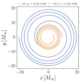
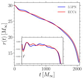
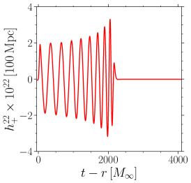
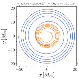
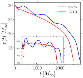
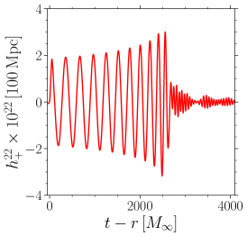
Figure 11: Same as in Fig. 5 when referring to extreme BNS configurations modelled with the TNTYST EOS (see also Fig. 10). The top row reports the orbital trajectories, the evolution of the proper separation after different eccentricity reductions, and the gravitational-wave strain for a irrotational BNS with mass ratio $q=0.455$. The bottom row reports the same quantities for a BNS with the same mass ratio but extreme spin asymmetry, $\chi_{1}=0,\chi_{2}=0.6$. Note that the large angular momentum of the spinning binary leads to more orbits and to a metastable merged object rather than to a black hole.

From there on, we follow the phase difference between the evolution as well as the ID resolutions compared to the highest resolution simulation. Both, the low evolution and ID resolution configurations are dominating the phase error in the early inspiral, while the higher resolution ID starts off with a significantly lower phase error. The slope of the growth of both contributions to the error over time is slightly differing and the evolution error is exceeding the accumulated errors from the low resolution ID towards merger, i.e., $\Delta\phi>1$. While the error using very low resolution ID is still comparable, using higher resolution ID leads to significantly smaller phase errors at merger when compared to the pure evolution error, being $\Delta\phi\approx 1$.

Overall, the result of these numerous simulations indicate that the error on the phase evolution introduced by the ID obtained with $\bar{N}\geq 38$ should be smaller than the typical error introduced by the evolution, especially for long inspirals. At the same time, increasing the ID resolution for evolutions at very high resolutions can improve the accuracy of the waveforms and yield a phase-evolution error that is $\Delta\phi\approx 1$. While a more thorough investigation covering larger portions of the parameter space is necessary for a precise picture of the error budget, it is already clear that that ID involving source terms like a perfect fluid demands higher evolution resolutions in general (cf. Sec. IV.2.2).

IV.3.4 Extreme mass ratios and spins

As a final capability test of the new BNS ID spectral-solver, we consider two configurations that are at the edges of the physically plausible space of parameters, thus generating two particularly extreme configurations. More specifically, we consider binaries built with the TNTYST tabulated EOS and create a first binary configuration at a separation of $30\,M_{\odot}$, with a mass ratio of $q=0.455$ and individual masses $M_{1}=2.2\,M_{\odot},M_{2}=1.0\,M_{\odot}$, so that the total mass of the binary is $M_{\infty}=3.2\,M_{\odot}$. To the best of our knowledge, this is represents the BNS configuration with the smallest mass ratio ever computed.

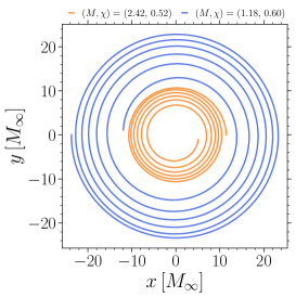
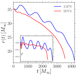
Figure 12: Same as in Figs. 5 and 11 but for a BHNS configuration. Note that the right panel reports the $\ell=m=2$ multipole the $\psi_{4}$ Weyl scalar [(both the real part (red solid line) and its norm (black solid line)] in order to highlight the very short ringdown that would not be visible in the gravitational-wave strain.

Given these masses, we create one BNS configuration with both stars being irrotational, i.e., $\chi_{1}=\chi_{2}=0$, and a corresponding configuration where the more massive companion is spinning extremely rapidly and the less massive component is nonspinning, i.e., $\chi_{1}=0.6,\chi_{2}=0.0$. This second BNS configuration could be seen as a realisation of a recycled binary pulsar in which one star gained a significant amount of matter and angular momentum through an exceptional accretion phase. It is important to remark that a binary configuration with unequal mass and unequal spins, as the one considered here, is more challenging to compute than when the masses are the same or when the spins are the same or, in general, of smaller magnitude.

Interestingly, despite this being a rather extreme configuration, the solver was able to generate this ID accurately and without any particular fixes or changes to the equations discussed in Sec. II.5. Indeed, already at a very low resolution of $\bar{N}=19$ we were able to generate a fully converged solution, which was successively scaled up directly to and resolved at a resolution of $\bar{N}=47$. Finally, before performing the evolution of these BNS configurations, we employed the iterative eccentricity reduction procedure using as reference the low-resolution dataset and thus reaching an orbital eccentricity of $\lesssim 10^{-4}$.

Figure 10 provides a direct measure of the properties of the two configurations by offering a cut through the $(x,y)$ and $(x,z)$ plane of the rest-mass density of the more massive star. The figure is organised in four panels, with the left column referring to the irrotational binary [$(x,y)$ plane on the top row and $(x,z)$ plane on the bottom row], while the right column reports the spinning binary. Also, we employ contour lines around the highest densities reached to help locate the most massive parts of the two stars and include small insets that are representations of the two binaries (the less massive companion is marked in red). As expected, the rapidly spinning star is strongly flattened, extending further out along on the equatorial plane and having a smaller extent along the $z$-axis. Furthermore, because of this distortion, the nuclear region of rest-mass density $\rho>10^{15}\,\rm{g/cm^{3}}$ is smaller as in the irrotational model, despite having the same $M_{{}_{\rm ADM}}$ at infinity.

We evolve both systems and present their trajectories in Fig. 11 following the same convention for the quantities reported in Fig. 5. Here, however, the top row refers to an irrotational binary, while the bottom row reports the same quantities for a BNS with extreme spin asymmetry, $\chi_{1}=0.6,\chi_{2}=0$. It is evident that the system with the highly spinning massive companion takes longer to merge. With the given fixed initial separation the difference amounts to approximately one orbit, which is due to the larger total angular momentum to be radiated away prior to the merger Kastaun et al. (2013); Dietrich et al. (2017); Ruiz et al. (2019); Most et al. (2019c). Finally, in the right panel of Fig. 11 we report the corresponding gravitational-waves strains in the $\ell=m=2$ mode and $+$ polarization. An important consideration to make here is that the binary system having the rapidly spinning companion is not collapsing promptly (red solid line in the right panel of Fig. 11), in contrast to what happens for the irrotational binary (black solid line), whose merged object collapses right after merger. This behaviour clearly suggests that spins can have a potentially important impact in determining the threshold mass to prompt collapse Bauswein et al. (2013); Koeppel et al. (2019) and thus need to be properly modeled to obtain accurate estimates of such masses over the entire physically relevant part of the space of parameters.

IV.4 Evolutions of black-hole–neutron-star binaries

As a final application of our new solvers and as an additional example of its flexibility, we consider the generation of ID representing a BHNS system. More specifically, we have considered a BHNS binary with a mass ratio of $q=0.485$ and a separation of $35.2\,M_{\odot}$ together with aligned spins of $\chi_{{}_{\rm BH}}=0.52$ and $\chi_{{}_{\rm NS}}=0.60$ (see also Most et al. (2020b)) utilising the TNTYST EOS Togashi et al. (2017) to model the nuclear matter. The initial orbital frequency $\Omega$ and the radial inward velocity of the orbit are fixed by the 3.5PN estimates given by Eqs.(74) and (75), using $M_{{}_{\rm ADM}}$ of the neutron star in isolation and $M_{{}_{\rm CH}}$ of the black hole as measured on the horizon. Although the two spins are neglected in these first estimates, they yield sufficiently reasonable initial guess with which to begin the eccentricity reduction procedure. Indeed, after performing four iterative steps, the final eccentricity of our binary is $\lesssim 10^{-3}$, where the resulting corrections for the first three steps of the iterative procedure were obtained using both the coordinate separation $r(t)$ and its derivative $\dot{r}(t)$. We note, however, that for eccentricities below $\sim 5\times 10^{-3}$, the corrections based on $r(t)$ lead to an increasingly eccentric orbit, so that the final (ECC4) ID dataset was obtained using estimates based on $\dot{r}(t)$ only.

In analogy with Figs. 5 and 11, we report in Fig. 12 the orbital trajectories, the evolution of the proper separation after different eccentricity reductions, and the gravitational-wave strain for the BHNS ID with mass ratio $q=0.485$. Note that the system undergoes six orbits in total and exhibits a very low residual eccentricity throughout the inspiral (middle panel). Furthermore, the center of mass that can be deduced already from the orbital tracks stays at the origin of the simulation domain, indicating a successful removal of the total residual linear momentum of the spacetime. Finally, note also that the gravitational-wave signal has a sharp cutoff after merger due to the disruption of the neutron star (this was remarked also in Ref. Foucart et al. (2020)). To highlight this behaviour and to reveal the ringdown, we do not report in the right panel of Fig. 12 the gravitational-wave strain in the $\ell=m=2$ multipole, but the corresponding multipole of the $\psi_{4}$ Weyl scalar [(both the real part (red solid line) and its norm (black solid line)]. It is clear that in this case the ringdown is very visible even if restricted to a couple of oscillations.

As a final remark we note that while our exploration of the space of parameters with the new solver is certainly very limited and aimed mostly at obtaining some reference solution, the calculation of BHNS ID has been successful for all of the cases we have explored and that have been restricted to black-hole spins $\chi\lesssim 0.75$, for which the conformal flatness is still a reasonable assumption. Moving to higher-spin black hole may require additional tuning since it is well known that the conformally flat background metric is not able to reliably reproduce highly spinning black-hole solutions (see Lovelace et al. (2008)).

V Discussion

A considerable effort has been dedicated in recent years to the construction of accurate and realistic initial data representing generic configurations of compact-object binaries in quasi-equilibrium. These configurations – which can either be of two black holes, of two neutron stars, or of a black hole and a neutron star – have then been employed for successful evolutions, starting from the early inspiral and well past merger. All of these simulations have enriched our understanding of merging binaries and helped in the interpretation of the signal from gravitational-wave detectors such as LIGO and Virgo.

While there are laudable examples of publicly available codes generating this type of initial data, these codes often provide only a limited capability in terms of mass ratios and spins of the components in the binary. In particular, there is at present no open-source code including the treatment of spinning neutron stars and an efficient procedure for the reduction of the initial eccentricity. In addition, there also exists a portion of the space of parameters – namely, the one considering the combination of extreme mass ratio and extreme and possibly differing spins for systems of binary neutron stars – that has, to date, not been explored in the context of constraint-satisfying initial data.

The work presented here aimed at filling this gap by providing an open-source collection of elliptic solvers that are capable of exploring a major part of the space of parameters relative to binary black holes (BBHs), binary neutron stars (BNSs), and mixed binaries of black holes and neutron stars (BHNSs). The starting point of our development has been the Kadath library, which is a highly parallelised spectral solver designed for numerical-relativity applicationsGrandclement (2010a). In addition, it is equipped with a layer of abstraction that allows equations to be inserted in a LaTeX-like format.

The set of elliptic equations employed for the calculation of the ID is well-known and has been presented in a number of related works. More specifically, we employ the extended conformal thin-sandwich method (XTCS), where the presence of a black hole is modeled by the usual excision approach using particular inner boundary conditions on the horizons, while the presence of a neutron star is modeled by either pure irrotational or with an additional rotational velocity contribution. By supporting both analytic EOSs, e.g., single polytropes and piece-wise polytropes, but also tabulated EOSs at zero or finite temperature, the new infrastructure is particularly geared towards allowing for the construction of BHNS and BNS binaries. For the latter, we showed that the new spectral solvers are able to reach the most extreme corners in the physically plausible space of parameters, including extreme mass ratios and spin angular momenta, the most extreme computed to date. For a first application of such extreme configurations with stellar companions close to their maximum mass $M_{{}_{\rm TOV}}$ see Most et al. (2020b). In this work we went even further and presented for the temperature-dependent TNTYST two BNS systems with an extreme mass asymmetry of $q=0.455$, a primary component with mass very close to the maximum mass i.e., $M_{1}/M_{{}_{\rm TOV}}>0.98$. These binaries are either irrotational or with large spin asymmetry, where the primary is very rapidly rotating with $\chi_{1}=0.6$. To the best of our knowledge, this is the most extreme BNS configuration computed to date.

As illustrated in terms of a systematic series of examples, the new spectral-solvers are able to construct quasi-equilibrium and eccentricity-reduced ID for BBHs, BNSs, and BHNSs, achieving spectral convergence in all cases. Furthermore, to assess the correctness of the newly constructed binary configurations, we have carried out evolutions of these systems from the inspiral to after the merger, obtaining in all cases a behaviour consistent with the expectations and previous results. An important aspect of these evolutions has been represented by the construction of ID that has only a minimal amount of initial eccentricity. The latter can be particularly large in the case of BNSs with small mass ratios and containing rapidly spinning companions, but is suitably reduced to acceptable values $\lesssim 10^{-4}-10^{-3}$ after employing an iterative eccentricity-reduction procedure, thus leading to accurate gravitational waveforms.

Finally, the evolution of the newly constructed ID has allowed us to obtain a partial first estimate of the error budget introduced by the finite resolution of the ID compared and to contrast it with the error introduced by the resolution employed for the solution of the evolution equations. While it is not in the scope of this paper to achieve a complete quantitative analysis of the impact in the case of different initial configurations, we have shown that the error budget contributed by the ID resolution on the gravitational-wave phase evolution is in general subdominant when compared to the errors introduced throughout the evolution, even for relatively low ID resolutions. Of course, these considerations only strictly apply to the configurations considered here and to the resolutions employed both for the ID and the evolution, which are, however, rather typical or real-life simulations of BHNS and BNSs.

Looking forward, there are multiple aspects of the spectral-solver library presented here that can be improved in the future. First, the current numerical setup inherits an assumed symmetry with respect to the $(x,y)$ plane, so that only spinning configurations with spins aligned or anti-aligned with the orbital angular momentum can be considered. There are at least two different ways to further generalize this setup and thus incorporate spin angular momenta that are not aligned along the $z$-direction: either by generalising the domain decomposition and relaxing the symmetry conditions enforced in the basis functions or by splitting the tensor fields into symmetric and anti-symmetric parts. Second, the system of equations is built and solved in the most straightforward way possible, and often this is not necessarily optimal. Considering that the Jacobian exhibits a structure that is known a priori and that the latter is partly sparse, more efficient nonlinear solvers could be employed, thus reducing the large memory demands and computational costs of solving the system using the full Jacobian. Third, the implementation of the black-hole boundary conditions could be generalized to use locally a Kerr spacetime background as done in Ref. Foucart et al. (2008), thus enabling the solver to cover the parameter space close to maximal black-hole spin angular momentum.

The official release of the codes are available on the Kadath website: https://kadath.obspm.fr.

Appendix A Eccentricity Reduction

To employ the eccentricity-reduction procedure mentioned extensively in the main text, we have essentially utilised the methods detailed in Refs. Buonanno et al. (2011); Foucart et al. (2008) as an effective manner to iteratively reduce the eccentricity of our binary ID. In essence, once a binary evolution is carried out and the distance between the two components – either a coordinate distance in the case of BBHs and BHNSs, or a proper distance in the case of BNSs – $r(t)$ and the corresponding time derivative $\dot{r}(t)$ are measured and fitted using the following ansatzes

$$r(t) =S_{r}(t)-\frac{B_{r}}{\omega_{r}}\cos(\omega_{r}t+\phi_{r})\,,$$ (68)

$$\dot{r}(t) =S_{r}(t)+B_{r}\sin(\omega_{r}t+\phi_{r}),$$ (69)

where $B_{r}$, $\omega_{r}$, and $\phi_{r}$ are fitting parameters from which it is possible to estimate the eccentricity $e$ as

$$e:=-\frac{B}{\omega_{r}d_{0}}\,,$$ (70)

with $d_{0}$ being the initial separation.

The function $S_{r}(t)$ in Eqs. (68) and (69) is freely specifiable and is used to fit, and hence remove any linear regression in the data while the periodic term is used to extract information regarding eccentricity induced oscillations in the orbit. In this work, we have used the following definition of $S_{r}(t)$ to produce the results described in Sec. IV

$$S_{r}(t) \equiv A_{0}+A_{1}t\,.$$

We have tested the use of quadratic terms in the expression for $S_{r}(t)$ and in the time dependencies of the oscillatory terms; however, this had a negligible impact on the fit parameters for the binary configurations considered in this work, hence prompting us to ignore these terms.

At each iteration, we use the fitting parameters $B_{r}$, $\omega_{r}$, and $\phi_{r}$ to estimate the corrections, $\delta\dot{a}$ and $\delta\Omega$, to $\dot{a}$ and $\Omega$ in Eq. (17) using

$$\delta\dot{a} :=-\frac{B\sin\phi}{d_{0}},$$ (71)

$$\delta\Omega :=-\frac{B\omega_{r}\cos\phi}{2\Omega d_{0}},$$ (72)

so that the new shift in Eq. (17) becomes

$$\beta^{i}_{{\rm cor}}=(\Omega+\delta\Omega)\partial^{i}_{\varphi}(\bm{x}_{c})+(\dot{a}+\delta\dot{a})r^{i}\,,$$ (73)

where the values of $\dot{a}$ and $\Omega$ are those obtained from the previous iteration.

This procedure is iterated until the eccentricity is reduced to an acceptable value, which, in all cases discussed in this work, was obtained with four iterations. Note that fits using $r(t)$ provide reasonable corrections until $e\approx 10^{-3}$. Attempting to reduce eccentricity below this threshold required the use of $\dot{r}(t)$ as the oscillations in $r(t)$ are too small to obtain an accurate fit.

Appendix B Post-Newtonian Estimates

In the post-Newtonian framework, the equations of motion describing circular motion in the center-of-mass frame corotating with the binary become much simpler (see Ref. Blanchet (2014), Sec 7.4). In particular, at the 3.5PN order, the quantities $\dot{a}$ and $\Omega$ can be expressed as

$$\dot{a}_{3.5\rm{PN}} =\frac{1}{r}\Bigg{[}-\frac{64}{5}\frac{M^{3}\nu}{r^{3}}\Big{(}1+\gamma\Big{(}-\frac{1751}{336}-\frac{7}{4}\nu\Big{)}\Big{)}\Bigg{]}\,,$$ (74)

$$\Omega^{2}_{3.5\rm{PN}} =\frac{M}{r^{3}}\Bigg{[}1+\Big{(}-3+\nu\Big{)}\gamma+\Big{(}6+\frac{41}{4}\nu+\nu^{2}\Big{)}\gamma^{2}+\Big{(}-10-\frac{75707}{840}+\frac{41}{64}\pi^{2}+22\ln\left(\frac{r}{r_{0}}\right)\nu+\frac{19}{2}\nu^{2}+\nu^{3}\Big{)}\gamma^{3}\Bigg{]}\,.$$ (75)

where $\mu:={M_{1}M_{2}}/{M_{\infty}}$ is the reduced mass,$\nu:=q/(1+q)^{2}=\mu/M_{\infty}$ is the symmetric mass ratio, $r$ is the (coordinate) separation between the centres of the two compact objects, and $r_{0}$ is the logarithmic barycentre defined by,

$$\ln r_{0} :=\frac{1}{M_{\infty}}\left(M_{1}\ln r_{1}+M_{2}\ln r_{2}\right)\,,$$ (76)

where $r_{1}$ and $r_{2}$ are the separation distances of the two compact objects relative to the center-of-mass.

We have therefore used Eqs. (74) and (75) to obtain initial estimates for these quantities and employed them, for instance, in the eccentricity-reduction procedure discussed in Appendix A. Perhaps a bit unexpectedly, we have found that the ID computed in this way provides a much better approximation to quasi-circular orbits of more challenging configurations than ID obtained assuming a quasi-equilibrium. This is even more surprising since the approximations (74) and (75) do not take into account spin or spin-orbit couplings. At the same time, it is important to underline that these estimates do require an accurate measurement of the center-of-mass to determine the radial position of each object relative to center-of-mass. Therefore, quasi-equilibrium is an important initial solution to obtain accurate PN estimates from Eqs. (74) and (75).

Additionally, Eqs. (77) and (78) have been used to compute the binding energy curves shown in Figs. 3 and 4

$$E_{b,3.5\rm{PN}} =-\frac{\mu x}{2}\Bigg{[}1+\Big{(}-\frac{3}{4}-\frac{1}{12}\nu\Big{)}x+\Big{(}-\frac{27}{8}+\frac{19}{8}\nu-\frac{1}{24}\nu^{2}\Big{)}x^{2}+\Big{(}-\frac{675}{64}+\Big{(}\frac{34445}{576}-\frac{205}{96}\pi^{2}\Big{)}\nu-\frac{155}{96}\nu^{2}$$

$$\phantom{=-\frac{\nu x}{2}\Bigg{[}}-\frac{35}{5184}\nu^{3}\Big{)}x^{3}\Bigg{]}\,,$$ (77)

$$E_{b,4\rm{PN}} =E_{b,3.5\rm{PN}}+-\frac{\mu x}{2}\Bigg{[}\Big{(}-\frac{3969}{128}+\frac{448}{15}\nu\ln x+e_{4}\nu+\Big{(}-\frac{498449}{3456}+\frac{3157}{576}\pi^{2}\Big{)}\nu^{2}+\frac{301}{1728}\nu^{3}+\frac{77}{31104}\nu^{4}\Big{)}x^{4}\Bigg{]}\,,$$ (78)

where $x:=\Omega^{{2}/{3}}$ and $e_{4}$ is the 4PN coefficient given by

$$e_{4}:=-\frac{123671}{5760}+\frac{9037}{1536}\pi^{2}+\frac{1792}{15}\ln 2+\frac{896}{15}e\,.$$ (79)