Quasinormal modes of slowly-rotating black holes in dynamical Chern-Simons gravity

Abstract

The detection of gravitational waves from compact binary mergers by the LIGO/Virgo collaboration has, for the first time, allowed us to test relativistic gravity in its strong, dynamical and nonlinear regime, thus opening a new arena to confront general relativity (and modifications thereof) against observations. We consider a theory which modifies general relativity by introducing a scalar field coupled to a parity-violating curvature term known as dynamical Chern-Simons gravity. In this theory, spinning black holes are different from their general relativistic counterparts and can thus serve as probes to this theory. We study linear gravito-scalar perturbations of black holes in dynamical Chern-Simons gravity at leading-order in spin and (i) obtain the perturbed field equations describing the evolution of the perturbed gravitational and scalar fields, (ii) numerically solve these equations by direct integration to calculate the quasinormal mode frequencies for the dominant and higher multipoles and tabulate them, (iii) find strong evidence that these rotating black holes are linearly stable, and (iv) present general fitting functions for different multipoles for gravitational and scalar quasinormal mode frequencies in terms of spin and Chern-Simons coupling parameter. Our results can be used to validate the ringdown of small-spin remnants of numerical relativity simulations of black hole binaries in dynamical Chern-Simons gravity and pave the way towards future tests of this theory with gravitational wave ringdown observations.

I Introduction

General Relativity (GR) has passed a plethora of experimental tests both in the Solar System Will (2014) and in binary pulsars systems Stairs (2003); Wex and Kramer (2020) making it one of the most successful physical theories. These tests probe situations in which gravitational fields are either weak, as in the Solar System, or systems where the field is strong but the system is slowly-varying, as in binary pulsars. However, the observation of gravitational waves (GW) by the LIGO/Virgo collaboration offers a new arena, where the spacetime is highly dynamical and strongly curved, in which the predictions of Einstein’s theory have being once more shown to agree with observations Abbott et al. (2016). Complementary, GW observations also allow one to constrain modifications to GR Yunes et al. (2016); Yagi and Stein (2016); Berti et al. (2018) and with more ground-based and space-based detectors in the future, these constraints will become more stringent (see e.g., Refs. Gnocchi et al. (2019); Toubiana et al. (2020); Perkins et al. (2021); Datta et al. (2021); Gupta et al. (2020)).

But why should one study modifications to GR? There are observational and theoretical anomalies that GR in its simplest form (i.e., without additional “dark” components or a UV completion) fails to answer. These include the late-time acceleration of the Universe Perlmutter et al. (1999); Riess et al. (1998), the anomalous galaxy rotation curves Sofue and Rubin (2001); Bertone and Hooper (2018) and the matter-antimatter asymmetry of the Universe Canetti et al. (2012) and the incompatibility of quantum mechanics with GR. A resolution to these anomalies may reside in a modification to Einstein’s theory that remains consistent with all current observational tests, yet yields deviations in other extreme regimes where the gravitational interaction is simultaneously strong, non-linear and highly dynamical. On the theoretical side, the incompatibility of GR with quantum mechanics has prompted efforts in a variety of unified theories, including string theory and loop quantum gravity.

These issues have served as motivation to study various extensions to GR Clifton et al. (2012); Berti et al. (2015), such as $f(R)$ gravity and scalar-tensor theories Sotiriou (2006); Kobayashi (2019), tensor-vector-scalar theories Skordis (2009), massive gravity de Rham (2014) and bi-gravity Schmidt-May and von Strauss (2016). Whether these attempts at modifying GR have any physical implications, requires one to first derive the predictions of such theories (in a given scenario) which should be followed by a comparison of these predictions against observations.

Although the correct completion of GR is yet unknown, GWs from compact binary coalescence observations can help in constraining and excluding entire arrays of modified theories of gravity. For instance, the GWs emitted in the inspiral of black hole binaries can tell us about the presence of extra radiative degrees of freedom, which provide an extra energy sink to which orbital energy and angular momentum can be extracted from the binary and hence affecting the system’s orbital evolution (see e.g., Ref. Berti et al. (2018)). Here we concentrate on GWs emitted when the newly formed black hole relaxes towards its final equilibrium state, the so-called ringdown. The GWs emitted during the ringdown can be described by a set of quasinormal modes (QNMs) – complex-valued frequencies whose imaginary part dictate how fast the mode decays in time. In GR, the observation of two or more QNMs in the ringdown signal allows one to uniquely infer the properties of the remnant Kerr black hole, similarly to how the observation of emission lines allows one to identify chemical elements Detweiler (1980). This “black hole spectroscopy” thus allows one to test the “Kerr hypothesis” Dreyer et al. (2004); Berti et al. (2006, 2007) i.e., that the BHs found in Nature are described by the Kerr metric. In general, modified theories of gravity do not admit the Kerr metric as a solution (see e.g. Ref. Berti et al. (2015)) and even when they do so Sotiriou and Faraoni (2012); Herdeiro and Radu (2015); Motohashi and Minamitsuji (2018), the presence of the modifications to GR can be probed by perturbations to the Kerr metric Barausse and Sotiriou (2008). This makes BH spectroscopy a powerful probe into beyond-GR physics.

Here we concentrate on modifications to GR which introduce a scalar field non-minimally coupled to squared curvature scalars, known as quadratic gravity theories Yunes and Stein (2011); Yagi et al. (2016). One subset of these theories, known as dynamical Chern-Simons (dCS) gravity Jackiw and Pi (2003), was proposed as an explanation to the matter-antimatter asymmetry of the universe by introducing additional parity-violating gravitational interactions, challenging a fundamental pillar of GR Alexander and Gates (2006); Alexander and Yunes (2009). The theory is poorly constrained by Solar System experiments (see Nakamura et al. (2019) for an overview), and remains unconstrained by both binary pulsars Yagi et al. (2013) and GWs Nair et al. (2019) observations. Nonetheless, first constraints on dCS were obtained through multi-messenger neutron star observations in Ref. Silva et al. (2020).

In dCS, nonrotating BHs are identical to their GR counterparts, but when spun a nontrivial scalar field configuration arises and whose presence affects the spacetime metric. Perturbations of spherically symmetric BHs in dCS were first studied in Ref. Yunes and Sopuerta (2008) who found the system of equation to be coupled and complicated. Later work decoupled these equations and studied them extensively Cardoso and Gualtieri (2009); Molina et al. (2010); Kimura (2018). Here we extend all of these results to axisymmetric, slowly-rotating BHs in dCS gravity and study their QNM spectra and stability.

Executive summary

We study the QNM spectra of slowly-rotating BHs in dCS gravity, generalizing Refs. Cardoso and Gualtieri (2009); Molina et al. (2010) which focused on the non-rotating case. To do so, we consider as a background the BH solution found in Refs. Yunes and Pretorius (2009); Konno et al. (2009) that captures the leading-order corrections due to the dimensionless spin ($a/M$) and Chern-Simons (CS) dimensionless coupling strength ($\alpha/M^{2}$) to the Schwarzschild spacetime. Here $a=J/M$ with $J$ and $M$ the Arnowitt-Deser-Misner angular momentum and mass respectively, while $\alpha$ is the coupling parameter (with dimensions of length squared in geometric units) between of the CS (pseudo-)scalar field and the Pontryagin density in the theory’s action.

We study the most general linear perturbations to this solution, taking into consideration both gravitational and scalar field perturbations. The outcome of this calculation is a pair of coupled, inhomogenous ordinary differential equations (ODEs) for the axial gravitational and scalar perturbations and a single homogeneous equation for the polar gravitational perturbations. All these equations are found to have CS modifications when compared with their counterparts for a slowly-rotating Kerr BH in GR Pani (2013).

With these equations in hand, we numerically calculate the QNM frequencies $\omega$, exploring their dependence on spin and coupling strength. We find that the QNM spectra can be split into two branches: (i) the scalar-led modes, whose frequencies in the limit $\alpha/M^{2}\to 0$ reduce to that of a test scalar field on a slowly-rotating Kerr BH background Witek et al. (2019); Pani (2013); Okounkova et al. (2019) and (ii) the gravitational-led modes, whose frequencies in the limit $\alpha/M^{2}\to 0$ reduce to that of the gravitational modes of a slowly-rotating Kerr background Pani (2013).

Our results show that the isospectrality existent in GR between axial and polar-parity gravitational modes Maggiore (2018) (i.e., the equivalence between the QNM spectra of each parity) is broken due to the scalar field. This was first observed in Molina et al. (2010) in the non-rotating limit and is shown here to persist when rotation is added. The leading order corrections to QNM frequencies introduced by the CS coupling are found to enter at the quadratic order in the CS coupling for both the gravitational and the scalar modes.

	$a/M$	$\alpha/M^{2}$
$\textrm{Re}(\omega_{g}^{\textrm{axial}})$	$\uparrow$	$\uparrow$
$\textrm{Im}(\omega_{g}^{\textrm{axial}})$	$\downarrow$	$\sim$
$\textrm{Re}(\omega_{s})$	$\downarrow$	$\downarrow$
$\textrm{Im}(\omega_{s})$	$\uparrow$	$\sim$
$\textrm{Re}(\omega_{g}^{\textrm{polar}})$	$\uparrow$	$\sim$
$\textrm{Im}(\omega_{g}^{\textrm{polar}})$	$\downarrow$	$\sim$

Table 1: Summary of the behavior of fundamental dominant QNM frequency as we increase either the dimensionless spin $a/M$ or the dimensionless CS coupling $\alpha/M^{2}$ while keeping the other constant. $\uparrow$, $\downarrow$ and $\sim$ indicate an increase, decrease or almost constant behavior of the QNM frequency, respectively. Here, the subscript $g$ represents the gravitational-led and the subscript $s$, the scalar-led mode.

We also found (at fixed spin $a/M$) that the axial gravitational modes decay slower and oscillate faster in dCS than in GR, with the latter being more sensitive to the CS coupling. We find a positive correlation between $a/M$ and $\alpha/M^{2}$ on how they affect the real part of the QNMs: the oscillation frequency increases in the same way by increasing either of the two parameters while keeping the other constant. This correlation is broken when considering decay rates, because changing the CS coupling has a negligible affect on the decay rate whereas a change in the spin parameter leads to longer lived modes. This result is important because it breaks the degeneracy between spin and CS coupling effects present in the real part of the QNM, allowing one to, in principle, constraint dCS gravity with the ringdown part of sufficiently high signal-to-noise-ratio GW events. At fixed spin, these corrections scale with $(\alpha/M^{2})^{2}$ due to dependence of the effective potential on the CS coupling and the coupling between the scalar and axial modes. In Table 1, we summarize how each of the three set of modes behave as we increase either spin or CS coupling while keeping the other constant.

We calculated a large set of QNM frequencies (see Appendix C) which we used to obtain fitting formulas for their real and imaginary parts as function of dimensionless spin and CS coupling [cf. Eqs. (54) and (54)]. Our exploration of the parameter space indicates that the QNMs decay for all values of spin and CS coupling within the limits of the slow rotation and small coupling approximation we use. This provides evidence that slowly rotating BH solutions in dCS gravity are linearly stable against gravito-scalar perturbations.

In the rest of this paper we show how these results were obtained. In Sec. II we give a short overview of dCS gravity and present the slowly-rotating BH solutions in this theory, whose QNM frequencies we are interested in computing. In Sec. III we review some general aspects of BH perturbation theory and derive the master equations that govern linear perturbations of our background BH spacetime. In Sec. IV we explain how these equations can be integrated numerically and in Sec. V we present our numerical results. Finally, in Sec. VI we summarize our main findings and discuss some avenues for future work.

We adopt the following conventions unless stated otherwise: we work in 4-dimensions with metric signature $(-,+,+,+)$ as in Misner et al. (1973). Greek indices ($\alpha,\beta....$) represent spacetime indices, round brackets around indices represent symmetrization, $\partial_{\mu}$ partial derivatives, $\nabla_{\mu}$ covariant derivatives and $\Box=\nabla_{\mu}\nabla^{\mu}$ the d’Alembertian operator. The Einstein summation convention is used throughout and we work in geometrical units in which $G=1=c$.

II Dynamical Chern-Simons Gravity

II.1 Basics

Let us start with a brief review of dCS gravity and establish some notation Alexander and Yunes (2009). In vacuum, the theory is described by the action

$$S=S_{{\mbox{\tiny EH}}}+S_{\vartheta}+S_{{\mbox{\tiny CS}}}\,,$$ (1)

where the Einstein-Hilbert term is

$$S_{{\mbox{\tiny EH}}}=\kappa\int d^{4}x\sqrt{-g}\;R\,,$$ (2)

where $\kappa=(16\pi)^{-1}$, $R$ is the Ricci scalar and $g$ is the determinant of the metric $g_{\alpha\beta}$. The action for the scalar field is

$$S_{\vartheta}=-\frac{1}{2}\int d^{4}x\sqrt{-g}\left[g^{\mu\nu}(\nabla_{\mu}\vartheta)(\nabla_{\nu}\vartheta)+2V(\vartheta)\right]\,,$$ (3)

where $\nabla_{\mu}$ is the covariant derivative operator compatible with the metric, while $V(\vartheta)$ is a potential for the scalar that we set to zero. The scalar field is nonminimally coupled to the Pontryagin density ${}^{*}\!RR$ as

$$S_{{\mbox{\tiny CS}}}=\frac{\alpha}{4}\int d^{4}x\sqrt{-g}\vartheta~{}^{*}\!RR\,,\,\,^{*}\!RR=~{}^{*}\!R^{\mu}{}_{\nu}{}^{\kappa\delta}R^{\nu}{}_{\mu\kappa\delta}\,,$$ (4)

where $\alpha$ is the CS coupling constant with units of [Length]² and ${}^{*}\!R^{\mu}{}_{\nu}{}^{\kappa\delta}$ is the dual Riemann tensor

$${}^{*}\!R^{\mu}{}_{\nu}{}^{\kappa\delta}=\frac{1}{2}\epsilon^{\mu}{}_{\nu\alpha\beta}~{}R^{\alpha\beta}{}^{\kappa\delta}\,,$$ (5)

and $\epsilon^{\mu\nu\alpha\beta}$ is the Levi-Civita tensor.

The field equations are obtained by varying the action in Eq. (1) with respect to the (inverse) metric $g^{\mu\nu}$ and scalar field $\vartheta$. Variation with respect to $g^{\mu\nu}$ gives

$$G_{\mu\nu}+\frac{\alpha}{\kappa}C_{\mu\nu}=\frac{1}{2\kappa}T^{\vartheta}_{\mu\nu}\,,$$ (6)

where $G_{\mu\nu}$ is the Einstein tensor, $C_{\mu\nu}$ is the (trace-free) C-tensor

$$C_{\mu\nu}=(\nabla_{\sigma}\vartheta)\epsilon^{\sigma\delta\alpha}{}_{(\mu}\nabla_{\alpha}R_{\nu)\delta}+(\nabla_{\sigma}\nabla_{\delta}\vartheta)~{}{}^{*}R^{\delta}{}_{(\mu\nu)}{}^{\sigma},$$ (7)

which contains derivatives of the scalar field, and $T^{\vartheta}_{\mu\nu}$ is the canonical scalar field stress-energy tensor

$$T^{\vartheta}_{\mu\nu}=\left[(\nabla_{\mu}\vartheta)(\nabla_{\nu}\vartheta)-\frac{1}{2}g_{\mu\nu}(\nabla^{\sigma}\vartheta)(\nabla_{\sigma}\vartheta)\right]\,.$$ (8)

Variation with respect to $\vartheta$ gives the inhomogenous wave equation

$$\Box\vartheta=-\frac{\alpha}{4}~{}^{*}\!RR\,.$$ (9)

One can show that ${}^{*}\!RR$ vanishes for static, spherically symmetric spacetimes, resulting in $\vartheta=\textrm{const.}$ as the only regular solutions of dCS in BH spacetimes with these symmetries Jackiw and Pi (2003); Yunes and Sopuerta (2008). This is no longer the case when these symmetries are lifted as we will see next.

Throughout this paper, we treat dCS gravity as a low energy effective field theory. What this means is that we will be working perturbatively in the coupling of the theory, considering only small deformations away from GR. Since this topic has been covered in literature in thorough detail, we redirect a reader unfamiliar with this topic to these references Alexander et al. (2021); Delsate et al. (2015); Motohashi and Suyama (2011, 2012).

II.2 Slowly-rotating black holes

Slowly-rotating BH solutions in dCS are known both analytically Konno et al. (2009); Yunes and Pretorius (2009); Yagi et al. (2012); Maselli et al. (2017) and numerically Delsate et al. (2018). Here we will consider the solution found in Refs. Yunes and Pretorius (2009); Konno et al. (2009), which was obtained by solving the field equations (6) and (8) perturbatively to linear order in spin $a$ and to quadratic order in the coupling strength $\alpha$. Following the notation of Yunes and Pretorius (2009), the line element of this solution is

$${d\bar{s}}^{2}=ds^{2}_{\mbox{\tiny SR}}+\frac{5}{4}\frac{\alpha^{2}}{\kappa}\frac{a}{r^{4}}\left(1+\frac{12}{7}\frac{M}{r}+\frac{27}{10}\frac{M^{2}}{r^{2}}\right)\sin^{2}\theta dtd\phi\,,$$

where $d\bar{s}^{2}$ is the background line element for the slowly rotating BH in dCS gravity to leading order in the dimensionless spin parameter and CS coupling constant and $ds^{2}_{\mbox{\tiny SR}}$ is the line element for a slowly-rotating Kerr BH

$$ds^{2}_{\mbox{\tiny SR}} =-f(r)dt^{2}-\frac{4Ma\sin^{2}\theta}{r}dtd\phi+f(r)^{-1}dr^{2}$$

$$\quad+r^{2}d\theta^{2}+r^{2}\sin^{2}\theta d\phi^{2}\,,$$ (11)

and $f(r)=1-2M/r$ is the Schwarzschild factor. The solution also contains a nontrivial scalar field,

$$\bar{\vartheta}=\frac{5}{8}\frac{a\alpha}{M}\frac{\cos\theta}{r^{2}}\left(1+\frac{2M}{r}+\frac{18M^{2}}{5r^{2}}\right)\,.$$ (12)

A far-field analysis shows that the BH has a scalar dipole charge of value $-(5/8)(a\alpha/M)$.

We see from Eq. (II.2) that the metric for slowly-rotating BHs in dCS gravity has an additional modification in the ($t\phi$)-component when compared to the metric in GR given in Eq. (II.2). This modifies the horizon angular frequency $\Omega_{{\mbox{\tiny H}}}$ as observed by a zero angular momentum observer at the horizon location $r_{\mbox{\tiny H}}$ at first order in spin and second order in $\alpha$ Yunes and Pretorius (2009) as

$$\Omega_{\mbox{\tiny H}}=\frac{a}{4M^{2}}-\frac{709\alpha^{2}a}{28672\kappa M^{6}}=\frac{a}{4M^{2}}\left(1-\frac{709}{7168}\zeta\right)\,,$$ (13)

where we defined

$$\zeta=\alpha^{2}/(M^{4}\kappa).$$ (14)

As we will see later, this $\alpha^{2}$-term affects the QNMs.

III Black Hole Perturbation Theory

III.1 Decomposition of the fundamental fields

We consider linear perturbations

$$g_{\mu\nu}=\bar{g}_{\mu\nu}+\epsilon\,\delta_{\mu\nu},\quad\vartheta=\bar{\vartheta}+\epsilon\,\delta\vartheta\,,$$ (15)

to the background BH spacetime [cf. Eqs. (II.2) and (12)], where $\epsilon$ is a bookkeeping parameter and both $\delta g_{\mu\nu}$ and $\delta\vartheta$ are functions of the coordinates of the metric.

The angular dependence of these perturbations can be described by scalar, vector and tensor spherical harmonics. The metric decomposition comes from the transformation properties of the ten components of the perturbation tensor $\delta g_{\mu\nu}$ under a rotation of the frame of origin Regge and Wheeler (1957). These quantities transform as three SO(2) scalars $\delta g_{MN}$, two SO(2) vectors $\delta g_{mN}$ and one SO(2) second rank tensor $\delta g_{ab}$ which can be expanded into a complete basis formed by spherical harmonics of different corresponding ranks. Under a parity transformation (i.e., the simultaneous shifts $\theta\to\pi-\theta$ and $\phi\to\phi+\pi$) the aforementioned metric quantities can be separated into odd (or “axial”) and even (or “polar”) sectors respectively, depending on whether they pick up a factor of $(-1)^{\ell+1}$ and $(-1)^{\ell}$. This allows us to decompose $\delta g_{\mu\nu}$ as

$$\delta g_{\mu\nu}(t,r,\theta,\phi)=\delta g^{\rm odd}_{\mu\nu}(t,r,\theta,\phi)+\delta g^{\rm even}_{\mu\nu}(t,r,\theta,\phi)\,,$$ (16)

where

$$\delta g^{\rm odd}_{\mu\nu}=\begin{pmatrix}0&0&h^{\ell m}_{0}(t,r)S^{\ell m}_{\theta}(\theta,\phi)&h^{\ell m}_{0}(t,r)S^{\ell m}_{\phi}(\theta,\phi)\\ *&0&h^{\ell m}_{1}(t,r)S^{\ell m}_{\theta}(\theta,\phi)&h^{\ell m}_{1}(t,r)S^{\ell m}_{\phi}(\theta,\phi)\\ *&*&0&0\\ *&*&*&0\end{pmatrix}\,,$$ (17)

and

$$\delta g^{\rm even}_{\mu\nu}=\begin{pmatrix}H_{0}^{\ell m}(t,r)Y_{\ell m}(\theta,\phi)&H_{1}^{\ell m}(t,r)Y_{\ell m}(\theta,\phi)&0&0\\ *&H_{2}^{\ell m}(t,r)Y_{\ell m}(\theta,\phi)&0&0\\ *&*&r^{2}K^{\ell m}(t,r)Y_{\ell m}(\theta,\phi)&0\\ *&*&*&r^{2}\sin^{2}\theta K^{\ell m}(t,r)Y_{\ell m}(\theta,\phi)\end{pmatrix}\,,$$ (18)

where the asterisk denotes symmetric components, $Y_{\ell m}(\theta,\phi)$ are the scalar spherical harmonics, while

$$S_{\theta}^{\ell m}(\theta,\phi) =-\frac{1}{\sin\theta}\partial_{\phi}Y_{\ell m}(\theta,\phi)\,,$$ (19)

$$S_{\phi}^{\ell m}(\theta,\phi) =\sin\theta\partial_{\theta}Y_{\ell m}(\theta,\phi)\,,$$ (20)

and a sum over $\ell$ and $m$ in the usual sense ($\ell\geqslant 0$ and $|m|\leqslant\ell$) is implicit. Equations (17) and (18) hold under the Regge-Wheeler gauge Regge and Wheeler (1957), which can be applied in theories with a massless graviton that support the usual two polarizations. In certain modified theories, a graviton can propagate with up to six polarizations, thereby leaving no residual gauge freedom. However, for the case of dCS gravity, GWs continue to propagate with only two polarizations (as measured at future null infinity) Sopuerta and Yunes (2009); Wagle et al. (2019), and thus, one retains enough gauge freedom to impose the Regge-Wheeler gauge. Such a decomposition separates the axial and polar perturbations with different harmonic index $\ell$, i.e., for a given $\ell$, we have two systems of evolution equations, one for the axial sector and one for the polar sector. These separate sets of equations completely characterize the linear response of the system.

Additional fields in the system, such as vectors and scalars, can be decomposed into spherical harmonics of the corresponding type. For scalar fields, we use scalar spherical harmonics and the perturbed scalar field reads

$$\delta\vartheta(t,r,\theta,\phi)=\frac{R_{\ell m}(r,t)}{r}Y_{\ell m}(\theta,\phi)\,.$$ (21)

III.2 Evolution equations for perturbations of a slowly rotating black hole

Having established the background spacetime and explained how the linear perturbations can be decomposed into scalar and tensor harmonics, we can now derive the perturbed form of the field equations in dCS gravity. The procedure is as follows:

• Substitute the linear perturbations (15) into the field equations (6) and (9) and expand to linear order in $\epsilon$.

• Expand the perturbed field equations to linear order in the spin parameter $a$ (slow-rotation approximation) and quadratic order in the coupling parameter $\alpha$ (small-coupling approximation).

• Use the orthogonality properties of the spherical harmonics presented in Appendix A to eliminate the angular dependence of the functions $A^{a}\in\{h_{0},h_{1},H_{0},H_{1},H_{2},K,R\}$, making them functions of $t$ and $r$ only. Moreover, assume an harmonic time-dependence in time, i.e.,

  $$A^{a}_{\ell m}(t,r)=e^{-i\omega t}A_{\ell m}^{a}(r)\,.$$ (22)

• The previous steps yields a system of 11 equations; 10 from the metric field equation (6) and one from the scalar field equation (9). The latter gives the evolution equation for the scalar field perturbations, whereas 3 of the metric equations reduce to the axial gravitational perturbation equation and the remaining 7 give an expression for the polar gravitational perturbation equation.

• This system of equations can then be expressed in general by an equation of the form

  $$\mathcal{D}\Psi_{j}+V_{j}\Psi_{j}=S_{j}[\Psi_{k},\partial_{r}\Psi_{k}]\,,$$ (23)

  where $j\in\{{\mbox{\tiny R}},{\mbox{\tiny RW}},{\mbox{\tiny ZM}}\}$, $k\in\{\{{\mbox{\tiny R}},{\mbox{\tiny RW}},{\mbox{\tiny ZM}}\}-j\}$ with $\{{\mbox{\tiny R}},{\mbox{\tiny RW}},{\mbox{\tiny ZM}}\}$ denoting the scalar, axial and polar gravitational perturbations respectively, $\mathcal{D}$ is a second-order radial differential operator, which in tortoise coordinates $(r_{*})$ reduces to $d^{2}/dr_{*}^{2}$, and $V_{j}$ is the effective potential. The source term $S_{j}$ is found to be a linear combination of the $\Psi_{k}$ master functions and its first radial derivatives, e.g. when $j={\mbox{\tiny R}}$, the master function $\Psi_{\mbox{\tiny R}}=R_{\ell m}$, and the source term $S_{\mbox{\tiny R}}$ is a function of $\Psi_{{\mbox{\tiny RW}}}$ and $\Psi_{{\mbox{\tiny ZM}}}$ and their first radial derivatives.

In the next subsections, we provide the final expressions for the perturbation equations for the scalar and gravitational sectors.

III.2.1 Scalar sector

The full equation describing the scalar field perturbation $R_{\ell m}$ is given by

$$f(r)^{2}\partial_{rr}R_{\ell m}+\frac{2M}{r^{2}}f(r)\partial_{r}R_{\ell m}+\left[\omega^{2}-V^{S}_{\rm eff}(r,a,\alpha^{2})\right]R_{\ell m}$$

$$=\alpha f(r)\left\{\left[g(r)+amh(r)\right]\Psi^{{\mbox{\tiny RW}}}_{\ell m}+amj(r)\partial_{r}\Psi^{{\mbox{\tiny RW}}}_{\ell m}\right\}$$

$$\quad+\alpha a\left\{q_{\ell m}\left[k_{1}(r)\Psi^{{\mbox{\tiny ZM}}}_{\ell-1,m}+k_{2}(r)\partial_{r}\Psi^{{\mbox{\tiny ZM}}}_{\ell-1,m}\right]\right.$$

$$\quad+\left.q_{\ell+1,m}\left[k_{3}(r)\Psi^{{\mbox{\tiny ZM}}}_{\ell+1,m}+k_{4}(r)\partial_{r}\Psi^{{\mbox{\tiny ZM}}}_{\ell+1,m}\right]\right\}\,,$$ (24)

where $f(r)=1-2M/r$,

$$q_{\ell m}=\sqrt{\frac{\ell^{2}-m^{2}}{4\ell^{2}-1}}\,,$$ (25)

and $\partial_{r}$ denotes radial derivatives. In Eq. (III.2.1), the functions $g$, $h$, $j$ and $k_{i}$ ($i=1,\dots,4$) also depend on $\ell$ and the mass of the black hole $M$ in addition to the radial coordinate. Their explicit forms are shown in Appendix B and in a Mathematica notebook Pra .

We also followed Pani (2013) and defined a CS modified Regge-Wheeler function $\Psi^{{\mbox{\tiny RW}}}_{\ell m}$, which to leading order in $a$ is given by

$$\Psi^{{\mbox{\tiny RW}}}_{\ell m}=\frac{f(r)}{r}\left(1+\frac{2mMa}{r^{3}\omega}-\alpha^{2}a\delta\Psi^{{\mbox{\tiny RW}}}(r)\right)h_{1}^{\ell m}\,,$$ (26)

where $h_{1}^{\ell m}$ comes from Eq. (17); the quantiy $\delta\Psi^{RW}(r)$ is a function of the radial coordinate included in the definition to allow us to maintain a form of the left hand side of Eq. (III.2.1) and other perturbed field equations similar to the form held by the Regge-Wheeler and Zerilli-Moncrief equation in GR. Similarly, we introduced the Zerilli-Moncrief function $\Psi^{{\mbox{\tiny ZM}}}_{\ell m}$, which to leading order in $a$ is given by

$$\Psi^{{\mbox{\tiny ZM}}}_{\ell m}=({z_{1}}/{z_{2}})-a({z_{3}}/{z_{4}})+\alpha^{2}a\delta\Psi^{{\mbox{\tiny ZM}}}(r)\,,$$ (27)

where

$$z_{1} =-2iH_{1}^{\ell m}(r-2M)+2K^{\ell m}r^{2}\omega\,,$$ (28a)

$$z_{2} =\left(6M+\lambda_{\ell}r\right)\omega\,,$$ (28b)

$$z_{3} =-4imM\omega\left[H_{1}^{\ell m}(r-2M)+iK^{\ell m}r^{2}\omega\right]$$

$$\quad\times\left\{48M^{3}-24M^{2}r+\lambda_{\ell}r^{3}(\lambda_{\ell}+2r^{2}\omega^{2})\right.$$

$$\quad+\left.2Mr^{2}\left(\lambda_{\ell}^{2}+6r^{2}\omega^{2}\right)\right\}\,,$$ (28c)

$$z_{4} =\ell(\ell+1)r^{4}z_{2}^{3}\,,$$ (28d)

with $\lambda_{\ell}=(\ell+2)(\ell-1)$, and $H_{1}^{\ell m}$ and $K^{\ell m}$ coming from Eq. (18). The quantity $\delta\Psi^{{\mbox{\tiny ZM}}}(r)$ serves a similar purpose to $\delta\Psi^{RW}(r)$. The forms of both $\delta\Psi^{RW}(r)$ and $\delta\Psi^{{\mbox{\tiny ZM}}}(r)$ are provided in a separate Mathematica notebook Pra .

III.2.2 Metric sector

The full equation describing the axial gravitational perturbation $\lambda_{\ell m}$ is given by

$$f(r)^{2} \partial_{rr}\Psi^{{\mbox{\tiny RW}}}_{\ell m}+\frac{2M}{r^{2}}f(r)\partial_{r}\Psi^{{\mbox{\tiny RW}}}_{\ell m}+\left[\omega^{2}-V^{A}_{\rm eff}(r,a,\alpha^{2})\right]\Psi^{{\mbox{\tiny RW}}}_{\ell m}$$

$$=\alpha f(r)\left\{\left[v(r)+amn(r)\right]R_{\ell m}+amp(r)\partial_{r}R_{\ell m}^{\prime}\right\}$$

$$+ a\left\{q_{\ell m}\left[p_{1}(r)\Psi^{{\mbox{\tiny ZM}}}_{\ell-1,m}+p_{2}(r)\partial_{r}\Psi^{{\mbox{\tiny ZM}}}_{\ell-1,m}\right]\right.$$

$$+ \left.q_{\ell+1,m}\left[p_{3}(r)\Psi^{{\mbox{\tiny ZM}}}_{\ell+1,m}+p_{4}(r)\partial_{r}\Psi^{{\mbox{\tiny ZM}}}_{\ell+1,m}\right]\right\}\,,$$ (29)

where the functions $v$, $n$, $p$ and $p_{i}$ ($i=1,\dots,4$) also depend on $\ell$ and $M$ in addition to the radial coordinate. Their explicit forms are given in Appendix B and in a Mathematica notebook available upon request.

Finally, the polar gravitational perturbation $Z_{\ell m}$ satisfies the equation

$$f (r)^{2}\partial_{rr}\Psi^{{\mbox{\tiny ZM}}}_{\ell m}+\frac{2M}{r^{2}}f(r)\partial_{r}\Psi^{{\mbox{\tiny ZM}}}_{\ell m}+\left[\omega^{2}-V^{P}_{\rm eff}(r,a,\alpha^{2})\right]\Psi^{{\mbox{\tiny ZM}}}_{\ell m}$$

$$=\alpha af(r)\left\{q_{\ell m}\left(s_{1}(r)R_{\ell-1,m}+s_{2}(r)\partial_{r}R_{\ell-1,m}\right)\right.$$

$$\quad+q_{\ell+1,m}\left.\left(s_{3}(r)R_{\ell+1,m}+s_{4}(r)\partial_{r}R_{\ell+1,m}\right)\right\}$$

$$\quad+a\left\{q_{\ell m}\left(r_{1}(r)\Psi^{{\mbox{\tiny RW}}}_{\ell-1,m}+r_{2}(r)\partial_{r}\Psi^{{\mbox{\tiny RW}}}_{\ell-1,m}\right)\right.$$

$$\quad+\left.q_{\ell+1,m}\left(r_{3}(r)\Psi^{{\mbox{\tiny RW}}}_{\ell+1,m}+r_{4}(r)\partial_{r}\Psi^{{\mbox{\tiny RW}}}_{\ell+1,m}\right)\right\}\,,$$ (30)

where the functions $s_{i}$ and $r_{i}$ ($i=1,\dots,4$) depend on $r$, $\ell$ and $M$. Their explicit forms are shown in Appendix B and in a Mathematica notebook Pra .

III.2.3 Selection rule and propensity rule

The perturbation equations (III.2.1), (III.2.2) and (30) show explicitly that $\ell$ modes couple to $\ell$ modes and $\ell\pm 1$ modes. However, as for slowly-rotating BHs in GR, these equations possess a selection rule Chandrasekhar and Ferrari (1991); Pani et al. (2012a). In GR and at linear order in spin, the selection rule is that the $\ell$-th axial (polar) mode couples to the $\ell\pm 1$ polar (axial) mode; at second order in spin, this simple selection rule needs to be modified Pani et al. (2012a). Similarly, in dCS gravity and at linear order in spin, the same selection rule applies to the perturbation equations. The only modification is that in dCS gravity we have two fields with axial parity: the scalar field (encoded in $R_{\ell m}$) and the Regge-Wheeler function (encoded in $\Psi_{\ell m}^{{\mbox{\tiny RW}}}$). Thus, in dCS gravity, $R_{\ell m}$ ($\Psi_{\ell m}^{{\mbox{\tiny RW}}}$) couples to $\Psi_{\ell m}^{{\mbox{\tiny RW}}}$ ($R_{\ell m}$) and to $\Psi_{\ell\pm 1,m}^{{\mbox{\tiny ZM}}}$, while $\Psi_{\ell m}^{{\mbox{\tiny ZM}}}$ couples to both $R_{\ell\pm 1,m}$ and $\Psi_{\ell\pm 1,m}^{{\mbox{\tiny RW}}}$.

In addition to this selection rule, the perturbation equations also suggest a propensity rule. More specifically, we see that when $\ell=|m|$, which dominates the linear response of the system, Eq. (25) yields $q_{\ell m}=0$, and thus the coupling of $\ell$ modes with $\ell-1$ modes is suppressed. This is similar in nature to the propensity rule of atomic physics, which states that transitions involving $\ell\to\ell+1$ are favored over those involving $\ell\to\ell-1$ Chandrasekhar and Ferrari (1991). Thus, we expect that the dominant modes are coupled only to the $\ell$ or the $\ell+1$ modes, after imposing the selection rule.

III.3 Simplification of the perturbation equations

Mode coupling between perturbation of different $\ell$-modes leads to a rich spectrum of solutions, but this paper is concerned with the QNM frequencies, which, as it turns out, are not affected by mode coupling to leading order in spin. Indeed, in GR this has been known since the 1990s, thanks to the work of Kojima and others Kojima (1993); Ferrari et al. (2007); Pani et al. (2012b, a). Let us then establish the same result in dCS gravity to leading order in spin and second order in coupling parameter. Without loss of generality, let us rewrite the perturbation equations as

$$A_{\ell m} +ma\tilde{A}_{\ell m}+a(q_{\ell}\hat{P}_{\ell-1,m}+q_{\ell+1}\hat{P}_{\ell+1,m})=0\,,$$ (31)

$$P_{\ell m} +ma\tilde{P}_{\ell m}\,+a(q_{\ell}\hat{A}_{\ell-1,m}+q_{\ell+1}\hat{A}_{\ell+1,m})=0\,.$$ (32)

In these equations, $A_{\ell m}$, $\tilde{A}_{\ell m}$ and $\hat{A}_{\ell\pm 1,m}$ are linear combinations of odd (axial) perturbations, which include the Regge-Wheeler function $\Psi_{\ell m}^{{\mbox{\tiny RW}}}$ and its derivatives, and also the scalar field perturbation $R_{\ell m}$ and its derivatives; we remind the reader that the scalar field perturbations are of odd (axial) parity as seen from Eq. (9). The prefactors of $\alpha^{0}$ and $\alpha^{1}$ have also been suppressed in the above functions for simplicity of notation. Similarly, $P_{\ell m}$, $\tilde{P}_{\ell m}$ and $\hat{P}_{\ell\pm 1,m}$ are linear combinations of polar perturbations encoded in the Zerilli-Moncrief function $\Psi_{\ell m}^{{\mbox{\tiny ZM}}}$ and its derivatives.

In GR, Kojima Kojima (1993) showed using symmetry arguments for the $m=0$ mode that the terms $\hat{P}_{\ell\pm 1,m}$ and $\hat{A}_{\ell\pm 1,m}$ in Eqs. (31) and (32) make no contribution to the QNMs. This argument was later extended to other values of $m$ in Ref. Pani et al. (2012a) for massive vector field perturbations of the slowly-rotating Kerr metric in GR. Following Ref. Pani et al. (2012a), we now extend this argument to slowly rotating BHs in dCS gravity.

Consider a simultaneous transformation,

$$x_{\ell,m}\to \mp x_{\ell,-m}\,, y_{\ell,m}\to \pm y_{\ell,-m}\,,$$

$$m\to -m\,, a\to -a\,,$$ (33)

where $x_{\ell m}$ and $y_{\ell m}$ represent the axial and polar perturbation variables respectively, with indices $(\ell,m)$ given in Eqs. (31) and (32) which remain invariant under such a transformation. The boundary conditions for QNMs of slowly rotating BHs in dCS (see Sec. IV.1) are also invariant under such transformation. Then, in the slow rotation limit, the QNM frequencies can be expanded as

$$\omega=\omega_{0}+ma\omega_{1}+a\omega_{2}+\mathcal{O}(a^{2})\,,$$ (34)

where $\omega_{0}$ is the eigenfrequency of the non-rotating BH in dCS gravity, which in our case is just a Schwarzschild BH. The effective potential presented in Sec. III.2 is proportional to $a^{0}$ and $ma$, but not to $a$ alone (see Appendix B). Hence, $\omega_{2}=0$, because the above potential would not source such a term.

The only terms that could source $\omega_{2}$, at least in principle, are $(\hat{P}_{\ell\pm 1,m},\hat{A}_{\ell\pm 1,m})$. This is because the second terms in Eqs. (31) and (32) are explicitly proportional to $m$, and because $(\tilde{A}_{\ell m},\tilde{P}_{\ell m})$ cannot be inversely proportional to $m$. Whether $(\hat{P}_{\ell\pm 1,m},\hat{A}_{\ell\pm 1,m})$ source $\omega_{2}$ depends on if they are independent of $m$ or not. However, since the second and third terms in Eqs. (31) and (32) are linear in $a$, both the functions $(\tilde{A}_{\ell m},\tilde{P}_{\ell m})$ and $(\hat{P}_{\ell\pm 1,m},\hat{A}_{\ell\pm 1,m})$ must be kept only to ${\cal{O}}(a^{0})$. Therefore, they correspond to perturbations of a non-rotating BH, which is necessarily spherically symmetric, implying in particular that $(\hat{P}_{\ell\pm 1,m},\hat{A}_{\ell\pm 1,m})$ are actually independent of $m$. But since $\omega_{2}$ vanishes by the arguments presented above, it follows that $(\hat{P}_{\ell\pm 1,m},\hat{A}_{\ell\pm 1,m})$ need not be included when computing the QNM spectrum.

Since the mode coupling terms can be neglected, our perturbation equations reduce to

$$f(r)^{2} \partial_{rr}R_{\ell m}+\frac{2M}{r^{2}}f(r)\partial_{r}R_{\ell m}+\left[\omega^{2}-V^{S}_{\rm eff}(r,a,\alpha^{2})\right]R_{\ell m}$$

$$=\alpha f(r)\left\{\left[g(r)+amh(r)\right]\Psi^{{\mbox{\tiny RW}}}_{\ell m}+amj(r)\partial_{r}\Psi^{{\mbox{\tiny RW}}}_{\ell m}\right\}\,,$$

$$f(r)^{2} \partial_{rr}\Psi^{{\mbox{\tiny RW}}}_{\ell m}+\frac{2M}{r^{2}}f(r)\partial_{r}\Psi^{{\mbox{\tiny RW}}}_{\ell m}+\left[\omega^{2}-V^{A}_{\rm eff}(r,a,\alpha^{2})\right]\Psi^{{\mbox{\tiny RW}}}_{\ell m}$$

$$=\alpha f(r)\left\{\left[v(r)+amn(r)\right]R_{\ell m}+amp(r)\partial_{r}R_{\ell m}\right\}\,,$$

$$f(r)^{2} \partial_{rr}\Psi^{{\mbox{\tiny ZM}}}_{\ell m}+\frac{2M}{r^{2}}f(r)\partial_{r}\Psi^{{\mbox{\tiny ZM}}}_{\ell m}+\left[\omega^{2}-V^{P}_{\rm eff}(r,a,\alpha^{2})\right]\Psi^{{\mbox{\tiny ZM}}}_{\ell m}$$

$$=0\,,$$ (35c)

where the values of all these functions are the same as before and are given in Appendix B.

Equations (35) can be recast in a Schrödinger-like form by introducing tortoise coordinates $r_{\ast}$,

$$r_{*}=r+2M\log\left(\frac{r}{2M}-1\right)\,.$$ (36)

However, when solving these equations, we will stick to the form given above to avoid confusion. Note in passing that the tortoise coordinate is typically used to map Schwarzschild coordinates to a horizon-penetrating (typically ingoing Eddington-Finkelstein) coordinate system, which is well adapted to imposing boundary conditions at the BH horizon. The standard transformation known in GR, however, may need to be modified by terms of ${\cal{O}}(\alpha^{2}a^{2})$ to transform a dCS BH to horizon-penetrating coordinates. Since we are here working to a lower order in perturbation theory, we do not need to worry about such details.

III.4 dCS coupling dependence of $\omega$ through a Fermi estimate

As seen from the previous section, for the calculation of the QNM frequencies, the perturbed equations take the form of Eqs. (35). In this subsection, we discuss the dependence of the QNM frequency $\omega$ on the dCS coupling parameter $\alpha$.

From Eq. (35), we see that the polar gravitational sector satisfies a homogeneous equation that lacks a direct coupling to the scalar field, although the effective potential $V_{\rm eff}^{P}$ is dependent on the CS coupling parameter $\alpha$. Thus, the QNM frequencies for the polar sector are proportional to second order in the CS coupling parameter. On the other hand, Eqs. (35) and (35) have a non-vanishing linear-in-$\alpha$ source term in addition to the effective potential having quadratic dependence on the CS coupling parameter.

What does this imply on the dCS corrections to the QNM frequencies $\omega$? We can answer this question with a Fermi estimate in which we replace any radial derivative by a characteristic radius $\partial_{r}\to 1/{\cal{R}}$ and evaluate the equation at this characteristic radius. Doing this in the perturbation equations (35) and (35) gives

$$\left[G({\cal{R}})+\omega^{2}-\left(V^{S}_{1}({\cal{R}})+\alpha^{2}V^{S}_{2}({\cal{R}})\right)\right]R_{lm}=\alpha H({\cal{R}})\Psi^{lm}_{{\mbox{\tiny RW}}}\,,$$ (37a)

$$\left[G({\cal{R}})+\omega^{2}-\left(V^{A}_{1}({\cal{R}})+\alpha^{2}V^{A}_{2}({\cal{R}})\right)\right]\Psi^{lm}_{{\mbox{\tiny RW}}}=\alpha I({\cal{R}})R^{lm}\,,$$ (37b)

where the effective potentials have been written as a linear combination of terms at zeroth and second order in CS coupling parameter and $G({\cal{R}}),H({\cal{R}}),I({\cal{R}})$ are polynomials in the radial coordinate $r$ evaluated at $r={\cal{R}}$, namely

$$G({\cal{R}}) =\frac{f({\cal{R}})^{2}}{r^{2}}+\frac{2Mf({\cal{R}})}{{\cal{R}}^{3}}\,,$$ (38)

$$H({\cal{R}}) =f({\cal{R}})\left[g({\cal{R}})+am\left(h({\cal{R}})+\frac{j({\cal{R}})}{{\cal{R}}}\right)\right]\,,$$ (39)

$$I({\cal{R}}) =f({\cal{R}})\left[v({\cal{R}})+am\left(n({\cal{R}})+\frac{p({\cal{R}})}{{\cal{R}}}\right)\right]\,.$$ (40)

Equations (37a) can be solved for $R_{\ell m}$ and then inserted into Eq. (37b), which leads to an equation for $\omega$ only, since $\Psi^{{\mbox{\tiny RW}}}_{\ell m}$ cancels and the $\omega$ dependence in $H({\cal{R}})$ and $I({\cal{R}})$ cancels when they are multiplied together. Doing so, one finds

$$\left[G+\omega^{2}-\left(V^{S}_{1}+\alpha^{2}V^{S}_{2}\right)\right] \left[G+\omega^{2}-\left(V^{A}_{1}+\alpha^{2}V^{A}_{2}\right)\right]$$

$$=\alpha^{2}I\,H\,,$$ (41)

where we have suppressed the argument of the functions. This is a quadratic equation for $\omega^{2}$, which we can solve perturbatively in $\alpha\ll 1$ to find

$$\omega=\omega_{{\mbox{\tiny GR}}}+\zeta\,\delta\omega+\mathcal{O}(\alpha^{3})\,,$$ (42)

where, recall, $\zeta=\alpha^{2}/(M^{4}\kappa)$ and

$$\omega_{{\mbox{\tiny GR}}} =\left(V^{A}_{\rm eff}-G\right)^{1/2}\,,$$ (43)

$$\delta\omega =\pm\frac{I\,H+(V^{A}_{1}-V^{S}_{1})V^{A}_{2}}{2\left(V^{A}_{1}-G\right)^{1/2}(V^{A}_{1}-V^{S}_{1})}\,.$$ (44)

One may worry that the above Fermi estimate for $\delta\omega$ may diverge because the denominator of Eq. (44) may vanish, but this does not occur anywhere outside the horizon. If we evaluate these expressions at ${\cal{R}}=3M$, which is close to where the effective potentials $V^{A}_{\rm eff}$ and $V^{S}_{\rm eff}$ are extremized, we find for the $\ell=2$ mode at $a=0$ that $M\omega_{{\mbox{\tiny GR}}}=1/3$ ($\approx 0.333$) and $M\delta\omega=-2/81$ ($\approx-0.025$), both of which are close to the real part of the correct numerical answers we will find later. The precise numerical factors, however, do not matter here. What matters is that the above Fermi estimate shows explicitly that the dCS corrections to the QNM frequencies will be of ${\cal{O}}(\alpha^{2})$. These corrections for the axial gravitational sector come from the second order correction to the effective potential as well as linear order coupling with scalar field.

Equation (42) also suggests that the QNM frequencies are even in the CS coupling. We have verified this with our numerical calculations shown in Sec. V by taking $\alpha\to-\alpha$ and found no change in the QNM frequency thereby supporting the results from the Fermi estimate.

IV Calculation of the Quasinormal Modes

The late-time GW signal from a perturbed BH is generally dominated by a sum of exponentially damped sinusoids known as the QNMs. These correspond to the characteristic vibrational modes of the spacetime Press (1971) and are complex valued. The real part represents the temporal oscillations whereas the imaginary part represents an exponentially decaying temporal part of the oscillations. Using the slowly-rotating approximation for finding QNMs of BHs allows us to use well-established numerical methods for their calculation. In this section, we show the boundary conditions and the numerical integration technique that will be used to calculate the QNMs.

IV.1 Boundary conditions

The QNMs are solutions of the inhomogeneous wave equations [Eqs. (35) to (35)] with appropriate boundary conditions. For the case of slowly-rotating BHs, we have two boundaries: one at spatial infinity and the other at the horizon $r_{\mbox{\tiny H}}$. The horizon of the BH described by the metric of Eq. (II.2) coincides with the Schwarzschild horizon (they are both located at $r=2M$ in Schwarzschild-like coordinates) at leading order in spin.

A QNM represents waves which are of purely ingoing at the horizon $r_{\mbox{\tiny H}}$ and purely outgoing at spatial infinity, which are characterized by complex frequency $\omega$ with ${\rm Re}(\omega)\geqslant 0$. These boundary conditions are,

$$\Psi_{j}\propto\bigg{\{}~{}\begin{matrix}e^{-i\omega_{\mbox{\tiny H}}r_{*}}\,,&r\to r_{\mbox{\tiny H}}\,,\\ e^{i\omega r_{*}}\,,&r\to\infty\,,\\ \end{matrix}$$ (45)

where recall that $\Psi_{j}=\{R_{\ell m},\Psi^{{\mbox{\tiny RW}}}_{\ell m},\Psi^{{\mbox{\tiny ZM}}}_{\ell m}\}$, $r_{*}$ is the tortoise coordinate and $\omega_{\mbox{\tiny H}}=\omega-m\Omega_{\mbox{\tiny H}}$, with $\Omega_{\mbox{\tiny H}}$, given by Eq. (13), is the horizon angular frequency for the BH under consideration.

IV.2 Evaluation of the QNMs: direct integration

To compute the QNMs, we use the direct integration method. In this method, we integrate the equations twice, once from finite distance outside the horizon towards spatial infinity, and once from a finite distance far from the horizon but inwards towards the event horizon. The integrations are started using the boundary conditions presented above, with a given choice of $\omega$. We then compare the two numerical solutions at a matching point $r_{m}$ that is somewhere between the horizon and spatial infinity, to check whether the master functions and their radial derivatives are continuous at $r_{m}$. Typically, this is not the case, so we then iterate this process over various values of $\omega$ until one finds a choice of the complex frequency that leads to continuous and differentiable solutions. In practice, this can be done by finding the value of $\omega$ for which the Wronskian $W$ of the two solutions vanishes at $r_{m}$ Maggiore (2018).

However, as simple as this approach appears, it is numerically difficult to implement due to inherent numerical instabilities. If one chooses the wrong value for $\omega$ then the trial integrations will tend to diverge as one approaches spatial infinity (for the outward solution) or as one approaches the BH horizon (for the inward solution). Also, since numerically we cannot start the integrations exactly at the horizon or at spatial infinity, the boundary conditions are not sufficiently accurate in general.

To improve numerical stability, one can improve the boundary conditions by finding analytic asymptotic solutions to the perturbation equations about spatial infinity and the horizon. More specifically, we can write Chandrasekhar and Detweiler (1975),

$$\Psi_{j}\propto\Bigg{\{}~{}\begin{matrix}e^{-i\omega_{\mbox{\tiny H}}r_{*}}\sum_{k=0}^{\infty}(\gamma_{k})_{j}(r-r_{\mbox{\tiny H}})^{k}\,,&r\to r_{\mbox{\tiny H}}\,,\\ \\ e^{i\omega r_{*}}\sum_{k=0}^{\infty}(\eta_{k})_{j}r^{-k}\,,&r\to\infty\,,\\ \end{matrix}$$ (46)

where the coefficients $\gamma_{k}$ and $\eta_{k}$ can be determined order by order in a series expansion of the perturbation equations around spatial infinity or the horizon. These coefficients can all be written entirely in terms of $(\gamma_{0})_{j}$ and $(\eta_{0})_{j}$, but they are long and not illuminating, so we will not present them in the paper, and instead they will be made available through a Mathematica notebook upon request. We will use these boundary conditions for our numerical integrations.

We will here compute the QNMs adapting the procedure in Blázquez-Salcedo et al. (2016) to our case. We begin by constructing two square matrices $W_{\rm o}$ and $W_{\rm e}$, which is four dimensional for the axial case due to the coupling between $\Psi^{{\mbox{\tiny RW}}}_{\ell m}$ and $R_{\ell m}$, and two dimensional for the polar case due to the lack of coupling. The columns of $W_{\rm o,e}$ are independent solutions of the perturbation equations, so

$$W_{\rm o} =\begin{pmatrix}{}_{{\mbox{\tiny H}}}\Psi^{{\mbox{\tiny RW}}\,(1)}_{\ell m}&{}_{{\mbox{\tiny I}}}\Psi^{{\mbox{\tiny RW}}\,(1)}_{\ell m}&{}_{{\mbox{\tiny H}}}\Psi^{{\mbox{\tiny RW}}\,(2)}_{\ell m}&{}_{{\mbox{\tiny I}}}\Psi^{{\mbox{\tiny RW}}\,(2)}_{\ell m}\\[5.0pt] \partial_{r}{}_{{\mbox{\tiny H}}}\Psi^{{\mbox{\tiny RW}}\,(1)}_{\ell m}&\partial_{r}{}_{{\mbox{\tiny I}}}\Psi^{{\mbox{\tiny RW}}\,(1)}_{\ell m}&\partial_{r}{}_{{\mbox{\tiny H}}}\Psi^{{\mbox{\tiny RW}}\,(2)}_{\ell m}&\partial_{r}{}_{{\mbox{\tiny I}}}\Psi^{{\mbox{\tiny RW}}\,(2)}_{\ell m}\\[5.0pt] {}_{{\mbox{\tiny H}}}R_{\ell m}^{(1)}&{}_{{\mbox{\tiny I}}}R_{\ell m}^{(1)}&{}_{{\mbox{\tiny H}}}R_{\ell m}^{(2)}&{}_{{\mbox{\tiny I}}}R_{\ell m}^{(2)}\\[5.0pt] \partial_{r}{}_{{\mbox{\tiny H}}}R_{\ell m}^{(1)}&\partial_{r}{}_{{\mbox{\tiny I}}}R_{\ell m}^{(1)}&\partial_{r}{}_{{\mbox{\tiny H}}}R_{\ell m}^{(2)}&\partial_{r}{}_{{\mbox{\tiny I}}}R_{\ell m}^{(2)}\\[5.0pt] \end{pmatrix},$$

$$W_{\rm e} =\begin{pmatrix}{}_{{\mbox{\tiny H}}}\Psi^{{\mbox{\tiny ZM}}}_{\ell m}&{}_{{\mbox{\tiny I}}}\Psi^{{\mbox{\tiny ZM}}}_{\ell m}\\[5.0pt] \partial_{r}{}_{{\mbox{\tiny H}}}\Psi^{{\mbox{\tiny ZM}}}_{\ell m}&\partial_{r}{}_{{\mbox{\tiny I}}}\Psi^{{\mbox{\tiny ZM}}}_{\ell m}\\ \end{pmatrix}\,,$$ (48)

where, the pre-subscript to the perturbation function ${}_{{\mbox{\tiny H}},{\mbox{\tiny I}}}\Psi$ denote whether the solutions is obtained by integration from the horizon to $r_{m}$, or from spatial infinity to $r_{m}$, while the superscripts $\Psi^{(1),(2)}$ denote two solutions evaluated with different initial conditions at the boundaries.

In principle, any set of independent solutions will do for the calculation of these $W_{\rm o,e}$ matrices, but in this paper we make the following choices. For the even sector, we choose the solution to be that obtained by integrating the perturbation equations with the boundary conditions in Eq. (46) and $[(\gamma_{0})_{{\mbox{\tiny ZM}}},(\eta_{0})_{{\mbox{\tiny ZM}}}]=(1,1)$. For the odd sector, we choose the two solutions to be those obtained by integrating with the boundary conditions in Eq. (46) and with $[(\gamma_{0})_{{\mbox{\tiny RW}}},(\eta_{0})_{{\mbox{\tiny RW}}},(\gamma_{0})_{{\mbox{\tiny R}}},(\eta_{0})_{{\mbox{\tiny R}}}]=(1,1,0,0)$ or with $[(\gamma_{0})_{{\mbox{\tiny RW}}},(\eta_{0})_{{\mbox{\tiny RW}}},(\gamma_{0})_{{\mbox{\tiny R}}},(\eta_{0})_{{\mbox{\tiny R}}}]=(0,0,1,1)$. In general, these solutions are linearly independent, unless $\omega$ is the correct QNM frequency, in which case

$${\rm det}(W)|_{r=r_{m}}=0\,.$$ (49)

We can use a root-finding algorithm to find the $\omega$ such that the Wronskian vanishes at the matching point.

Using this method, we have calculated the QNMs of a slowly-rotating BH in dCS gravity. In practice, all numerical integrations that start at the horizon are initiated at $r_{\rm initial,r_{+}}=(2+10^{-4})M$, while those that start at spatial infinity are initiated at $r_{\rm initial,i_{0}}=60M$, with the matching always performed at $r_{m}=20M$. We have checked the numerical stability of the QNM frequencies against changes in the values of $r_{\rm initial,r_{+}}$, $r_{\rm initial,i_{0}}$ and $r_{m}$. All numerical integrations are done with the NDSolve package of Mathematica, with accuracy and precision set to 10 digits.

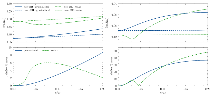
Figure 1: Comparison between the fundamental dominant $\ell=m=2$ gravitational and scalar QNMs calculated using the exact Kerr metric and its expansion to leading-order in $a$. The dependence of the real (imaginary) part of the frequency on the spin $a$ is shown in the left (right) top panel. The left (right) bottom panel shows the relative error defined by Eq. (52). The colors distinguish the scalar (green) and gravitational (blue) QNMs. Unsurprisingly, we see that the relative percent error $\delta\omega$ increases with spin $a/M$, doing so faster for the imaginary part of the frequency, although the absolute error is $\mathcal{O}(a^{2})$. The legends shown in the left panels apply to the corresponding right panels as well.

V Numerical Results

In this section, we present our numerical results for the QNM frequencies. For clarity, we have divided this section into three parts. First, we take the GR limit (i.e., $\alpha/M^{2}=0$) of our equation and discuss the associated QNMs of a slowly-rotating Kerr BH with the metric expanded to leading-order in spin. We compare these results with the exact Kerr QNMs obtained using Leaver’s continued fraction method Leaver (1985). This preliminary step will give us an estimate of where the slow-rotation approximation breaks down and how the numerical errors due to this approximation compare against the modifications to the QNM frequencies due to the CS coupling. Second, we consider a nonzero CS coupling $\alpha/M^{2}$ and study in detail how the QNMs behave as functions of this coupling and of the BH spin. Third, we construct fitting formulas for the real and imaginary parts of the QNMs, valid within the errors associated to the slow-rotation approximation.

In the main body of this paper, we will show numerical results for the fundamental $n=0$, $\ell=m=2$ frequencies since these are dominant for tensorial perturbations. We leave our results for the QNM frequencies for the fundamental mode with $\ell=2$, $\ell=3$ and $\ell=4$ modes, and all $m$ modes to Appendix C. To aid in the presentation of these numerical results, we will work with dimensionless parameters by rescaling $a$, $\alpha$ and $\omega$ as

$$a\to a/M,\quad\alpha\to\alpha/M^{2},\quad\textrm{and}\quad\omega\to\omega M\,.$$ (50)

In our numerical calculations, we work in code units, in which $M=1$, thus making the code quantities $a$, $\alpha$ and $\omega$ dimensionless.

V.1 Slow rotation: GR

The calculation of the QNMs of a slow-rotating Kerr BH in GR were presented in Pani (2013), but to our knowledge a comparison between these results and those obtained using the exact Kerr metric has not appeared in the literature. See Maselli et al. (2020); Hatsuda and Kimura (2020) for complementary studies. This comparison is important for our purposes for two reasons. First, it will tell us up to what values of $a$ we can trust our slow-rotation approximation. Second, it will tell us whether the errors due to this approximation are degenerate with modifications to the GR QNMs introduced by the CS coupling. We refer the interested reader to Ayzenberg et al. (2016) for a similar analysis, but in a different context.

In the GR limit ($\alpha/M^{2}=0$) the perturbation equations [cf. Eqs. (III.2.1), (III.2.2) and (30)] decouple and each of them reduces to equations of the form

$$f(r)^{2}y^{\prime\prime}_{\ell m}+(2/r^{2})f(r)y^{\prime}_{\ell m}+[\omega^{2}+v_{\rm eff}(r,a)]y_{\ell m}=0\,,$$ (51)

for the field variables and effective potential pairs $\{y_{\ell m},\,v_{\rm eff}\}=\{R_{\ell m},\,V^{S}_{\rm eff}\}$, $\{\Psi^{{\mbox{\tiny RW}}}_{\ell m},\,V^{A}_{\rm eff}\}$ and $\{\Psi^{{\mbox{\tiny ZM}}}_{\ell m},\,V^{P}_{\rm eff}\}$. For the gravitational perturbations these equations agree with those in Pani (2013), whereas for the scalar perturbation they agree with the small-$a$ limit of that in Brill et al. (1972). Moreover, in this limit, the axial and the polar gravitational equation become isospectral.

As a benchmark for our numerical code, we calculated the gravitational and scalar QNMs of a Schwarzschild BH by taking the nonrotating limit ($a=0$). We find excellent agreement with the well-known result summarized e.g. in Berti et al. (2009); Ber . Next, we computed the QNMs associated with Eq. (51) and compared them against the QNMs obtained using the exact Kerr metric (i.e., without performing any small-$a$ expansion) by means of the continuous fraction method Leaver (1985) and tabulated in Berti et al. (2009); Ber

Figure 1 presents the results of this exercise, focusing on the fundamental mode with $\ell=m=2$. The top panels show a comparison between the behavior of the real (left) and the imaginary (right) parts of the QNM frequencies for the slowly-rotating Kerr metric (solid) and the exact Kerr metric (dashed) as a function of the spin parameter $a$ for both the scalar (green curves) and the gravitational modes (blue curves). The bottom panels show the relative percent error due to the slow rotation approximation, which we define via

$$\delta(\rm{Im}\,\omega) =\left|1-(\rm{Im}\,\omega_{{\mbox{\tiny SR}}})/(\rm{Im}\,\omega_{{\mbox{\tiny K}}})\right|\times 100\,,$$ (52a)

$$\delta(\rm{Re}\,\omega) =\left|1-(\rm{Re}\,\omega_{{\mbox{\tiny SR}}})/(\rm{Re}\,\omega_{{\mbox{\tiny K}}})\right|\times 100\,,$$ (52b)

where, $\omega_{{\mbox{\tiny K}}}$ are the QNM frequencies calculated from the exact Kerr metric Leaver (1985); Berti et al. (2009), whereas $\omega_{{\mbox{\tiny SR}}}$ are the QNM frequencies we calculated for the Kerr metric expanded to linear order in $a/M$.

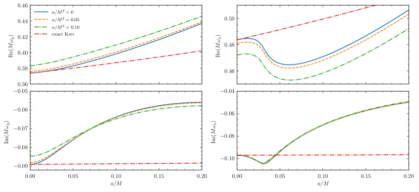
Figure 2: Real (Imaginary) parts of the QNM frequencies for the $n=0$, $\ell=m=2$ mode as a function of the spin parameter for slowly rotating BHs in dCS gravity with different CS couplings $\alpha/M^{2}$ are shown in the top (bottom) panels for the axial gravitation-led (left) and scalar-led (right) modes. Additionally, we have also shown the exact Kerr QNMs for BHs in GR for quick comparison calculated in Berti et al. (2009). The individual QNM frequencies increase for the gravitational-led modes with spin parameter $a/M$ as well as with the CS coupling $\alpha/M^{2}$, whereas the scalar-led modes increase with spin parameter, but decrease with the CS coupling. The imaginary part of $M\omega_{g}^{\rm axial}$ decreases slightly in magnitude with increasing $\alpha/M^{2}$ for spins $a/M\lesssim 0.06$, while it increases slightly in magnitude for spins $a/M\gtrsim 0.06$. Since our slow-rotation approximation is valid up to spin values of approximately at most $0.04$, overall these modes become less damped in dCS gravity. The legends apply to all panels.

We can extract several conclusions from this figure. First, the relative error introduced by the slow-rotation approximation is larger for the imaginary part of the frequency than for the real part. For instance, when $a/M=0.1$, the relative error is approximately eight times larger on the imaginary part than on the real part for both gravitational and scalar-led modes. In addition, we also find that the absolute error $|\omega_{{\mbox{\tiny SR}}}-\omega_{{\mbox{\tiny K}}}|$ is of $\mathcal{O}(a^{2})$ for both the real and imaginary parts of the QNM frequencies. This naturally follows from the fact that the error should indeed be of $\mathcal{O}(a^{2})$, since we have evaluated $\omega$ to leading order in the spin parameter. The results show that the approximation introduces errors smaller than $10\%$ when $a/M\lesssim 0.2$ for the real part and $a/M\lesssim 0.04$ for the imaginary part. Here, we have not included the errors due to our numerical integration scheme since the total error is dominated by the error introduced in the slow rotation approximation.

V.2 Slow rotation: dCS

In this subsection, we show how the QNM frequencies discussed in the previous subsection are modified by the presence of a nonzero CS coupling $\alpha/M^{2}$ for the dominant $n=0$, $\ell=m=2$ mode. Tabulated values for the QNM frequencies for the fundamental mode with $\ell=2,~{}\ell=3,~{}$ and $\ell=4$ and all $m$ can be found in Appendix C.

As we discussed in Sec. III.2.3, our calculations are valid to linear order in spin $a/M$, but second-order in the CS coupling $\alpha/M^{2}$. Recall that the polar QNM frequencies [governed by Eq. (35)] are independent of the coupling with the scalar field or with the axial parity sector due to the dependence of the effective potential on the CS coupling  Cano et al. (2020). We therefore focus on the coupled system of Eqs. (35) and (35) and the Eq. (35) separately and use the numerical procedure described in Sec. IV to calculate the QNMs in different parity sectors.

V.2.1 Axial gravitational and scalar sector

Our results for the fundamental modes are summarized in Figs. 2 and 3.

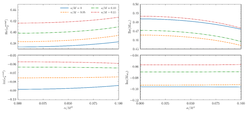
Figure 3: Real (Imaginary) parts of of the QNM frequencies as a function of the CS coupling for slowly rotating BH in dCS gravity for different values of the spin parameter $a$ are shown in the top (bottom) panels for the gravitational-led (left) and scalar-led (right) modes. We see that increasing the spin $a/M$ shifts the curves upward in all panels. In addition, we see that the real part of $M\omega_{g}^{\rm axial}$ increases as we increase the CS coupling, whereas it decreases for the real part of $M\omega_{s}$. This is behavior happens for all constant-spin curves. For higher spins, we see that the changes to the decay rates are negligible as the CS coupling is increased for both sectors. This behavior may be a consequence of the slow rotation approximation we use. Finally, for a fixed value of spin, the curves exhibit a quadratic order dependence on the CS coupling supporting our estimate in Sec. III.4. The legends apply to all panels.

In Fig. 2 we show the dependence of the real and imaginary values of gravitational- and scalar-led QNMs as function of spin parameter $a/M$ for $\alpha/M^{2}=\{0,0.05,0.10\}$. In Fig. 3 we complement this analysis, by showing the dependence of the QNMs on $\alpha/M^{2}$ for $a/M=\{0,0.05,0.10,0.15\}$. These two figures can be thought of as showing the slow-rotation corrections to the non-rotating BH QNM frequencies in dCS and the dCS modifications to the GR QNM frequencies respectively.

As seen from Figs. 2 and 3, the behaviors of the real and the imaginary part for gravitational-led and the scalar-led sectors are distinct. Thus, we present individual analysis for each.

• Real gravitational-led QNM (top left panel of Figs. 2 and 3). The $\textrm{Re}(\omega_{g}^{\rm axial})$ increases with BH spin just as in GR (see Sec. V.1) for constant CS coupling, and it increases as the CS coupling increases for constant spin.

• Imaginary gravitational-led QNM (bottom left panel of Figs. 2 and 3). The $\textrm{Im}(\omega_{g}^{\rm axial})$ decreases with BH spin for a constant CS coupling just like in GR, whereas it remains constant with increasing CS coupling for a constant spin.

• Real scalar-led QNM (top right panel of Figs. 2 and 3). The $\textrm{Re}(\omega_{s})$ initially shows a sinusoidal behavior as we increase spin and hold the CS coupling constant up to $a=0.05$, and then it increases with BH spin. On the other hand, the $\textrm{Re}(\omega_{s})$ decreases monotonically with the CS coupling while keeping the BH spin constant.

• Imaginary scalar-led QNM (bottom right panel of Figs. 2 and 3). The $\textrm{Im}(\omega_{s})$ initially increases with BH spin for constant CS coupling, reaches a minimum and then decreases again. On the other hand, the $\textrm{Im}(\omega_{s})$ remains essentially constant as we change the CS coupling for constant spin.

Figures 2 and 3 shows that the real part of QNM frequencies has a similar functional behavior with spin, for different values of the CS coupling. These frequencies depend quadratically on the CS coupling, as required by the order reduction scheme employed in this paper (see e.g. Ref. Yunes and Pretorius (2009)), which is also displayed in the figures.

The modes presented above show a non-monotonic behavior with respect to the spin parameter in contrast with the equations being linear in this parameter. This is mainly because the equations (35) are nonlinear in the QNM frequency $\omega$ (this can be seen explicitly from the occurrences of $\omega$ in the various functions these equations). Since we are not linearizing $\omega$ with respect to the spin parameter to avoid loss of information from the equations, we obtain a nonlinear behavior for the QNM frequencies of the gravitational-led modes and, more evidently, for the scalar-led modes.

These results have interesting implications for GW observations. GW detectors will be sensitive directly only to the gravitational wave modes, not the scalar modes. Focusing on the real part of $\omega_{g}^{\rm axial}$, we then see that there is a degeneracy through a positive correlation between $\alpha$ and $a$; increasing $a$ while keeping $\alpha$ constant has the same effect as increasing $\alpha$ while keeping $a$ constant. However, this correlation breaks when considering the imaginary part of $\omega_{g}^{\rm axial}$; increasing $a$ leads to longer lived modes (smaller imaginary frequencies) for constant $\alpha$, while increasing $\alpha$ does not change much the lifetime for constant $a$. This then suggests that, in principle it may be possible to separate the effects of spin and CS coupling parameter given a ringdown observation that is loud enough.

V.2.2 Polar gravitational sector

The results for the fundamental modes for the polar gravitational sector is summarized in Fig. 4. We show the dependence of the real and imaginary values of polar gravitational QNMs as a function of spin parameter $a/M$ for $\alpha/M^{2}=\{0,0.05,0.10\}$. Tabulated values for the QNM frequencies for the fundamental mode with $\ell=2$ and $\ell=3$ and $\ell=4$ for all $|m|\leqslant\ell$ can be found in Appendix C.

As seen from Fig. 4, the behavior of the real and the imaginary part for polar gravitational sector is distinct. Therefore, we present individual analysis for each.

• Real gravitational-led QNM (left panel of Fig. 4). The $\textrm{Re}(\omega_{g}^{\rm polar})$ increases with BH spin just as in GR (see Sec. V.1) for constant CS coupling, while it remains almost constant as the CS coupling increases for constant spin.

• Imaginary gravitational-led QNM (right panel of Fig. 4). The $\textrm{Im}(\omega_{g}^{\rm polar})$ decreases with BH spin for a constant CS coupling just like in GR, whereas it remains almost constant with increase in CS coupling for a constant spin.

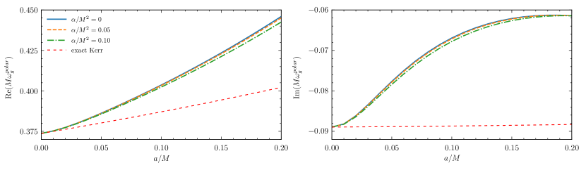
Figure 4: Real (left panel) and imaginary parts (right panel) of the QNM frequencies for the $n=0$, $\ell=m=2$ polar gravitational-led mode as functions of the spin parameter for slowly rotating BHs in dCS gravity with different CS couplings $\alpha/M^{2}$. We have also shown the exact Kerr QNMs for BHs in GR for comparison taken from Berti et al. (2009). The individual QNM frequencies increase for the polar gravitational-led modes with spin parameter $a/M$, but decrease slightly with the CS coupling $\alpha/M^{2}$. The imaginary part is also almost constant in magnitude with increasing $\alpha$, suggesting that damping of modes is almost independent of the CS coupling. The legends apply to all panels.

The modes decay for all values of spin parameter and CS coupling within the limits of our approximation, giving strong evidence that slowly-rotating BHs in dCS gravity are linearly stable against gravito-scalar perturbations, extending the results of Molina et al. (2010); Kimura (2018) to small spins.

V.2.3 Regime of validity of numerical results and implications

In interpreting the figures, especially Fig. 2, one must be careful to take into account the approximate nature of our results. The numerical calculations we have performed are only valid in the slow-rotation approximation (to leading order in the BH spin and second order in the CS coupling). This is why we included a discussion in Sec. V.1, which quantify approximately the error in the slow-rotation approximation. When the spin is large enough that this error becomes comparable to the dCS correction, then our numerical results should not be trusted any longer. This occurs roughly at $a/M\gtrsim 0.2$ for $\textrm{Re}(\omega_{g,s})$, $a/M\gtrsim 0.05$ for $\textrm{Im}(\omega_{g})$ and $a/M\gtrsim 0.07$ for $\textrm{Im}(\omega_{s})$, for both axial or polar modes due to their isospectrality, where we have a maximum relative error of around $10\%$ due to the slow rotation approximation as shown in Fig. 1. Therefore, to be conservative, henceforth we restrict our attention to the regime $a/M\leqslant 0.0375$, where the errors introduced by the slow-rotation approximation are very small and the dCS corrections we have calculated are meaningful.

Our results allow us to estimate the magnitude of the dCS deviations with respect to the GR QNMs. As an example, let us saturate the best constraint to date on the CS coupling parameter, $\alpha^{1/2}\leqslant 8.5$ km (at 90% confidence), obtained in Silva et al. (2020), and consider the smallest remnant BH mass observed so far ($M\approx 18\,M_{\odot}$), the product of the event GW170608 Abbott et al. (2017). Combining this value of $M$ with the maximum value of $\alpha$ allowed from Silva et al. (2020), we find $\alpha/M^{2}\approx 0.1$. We can now use the data presented in Tables 4 and 5 (see also Fig. 2) to find that the maximum deviations from the GR QNMs is about $2\%$ ($2\%$) for the oscillation frequency and about $9\%$ ($6\%$) for the decay rate for the fundamental dominant $\ell=m=2$ axial gravitational- (scalar-) led modes and a BH with spin $a/M=0.0375$ (i.e., at the upper limit of our slow-rotation approximation).

Let us re-iterate that a GW detector responds only to gravitational degrees of freedom that propagate from the source to the detector (taken to be at spatial infinity), which in dCS gravity was shown to consist of the standard “plus” and “cross” transverse-traceless polarization modes, just as in GR Wagle et al. (2019). This means that in practice only deviations to the gravitational-led modes can be used to test dCS gravity, since these are the modes that affect the detector. To constrain the modest deviations predicted here one would require a very high signal-to-noise ratio event, in addition to detection and characterization of at least two ringdown modes (to break degeneracies between mass, spin and dCS coupling). One should bear in mind however, that the small deviations found here may be a consequence of the small-spin approximation. For BHs in dCS gravity, the larger the spin, the larger the deformations away from the Kerr metric become, which in turn may reflect on larger deviations in the QNM frequencies. This implies that tests of dCS gravity through BH spectroscopy would benefit from an extension of our work to larger spin values.

V.3 Fitting formulas for the QNMs

We have calculated a large catalog of QNM frequencies from which we can construct ready-to-use fitting formulas for the fundamental mode with $\ell=m=2$, as well as other multipoles. This catalog allows for the fast evaluation of QNM frequencies without having to redo the numerical calculations, which are computationally non-trivial, requiring approximately $20$ hours of CPU time per curve in the figures above. We first focus our attention on the axial gravitational- and scalar-led modes. For a given value of $\alpha$, and a given value of $n$, $\ell$ and $m$, let us use the fitting functions

$$M\omega_{g}(M,a) =a_{g}+b_{g}\left(1-a/M\right)^{c_{g}}\,,$$ (53a)

$$M\omega_{s}(M,a) =a_{s}+b_{s}\left(1-a/M\right)^{c_{s}}\,,$$ (53b)

where $(a_{g},b_{g},c_{g})$ and $(a_{s},b_{s},c_{s})$ are fitting coefficients for the axial gravitational-led and the scalar-led sectors of the QNMs, respectively. Table 2 presents the numerical values of these coefficients for the fundamental dominant $n=0$, $\ell=2$, $m=2$ mode, and selected values of the CS coupling $\alpha/M^{2}$.

The fitting coefficients show a quadratic dependence on $\alpha$, in agreement with the arguments presented in Sec. III.4. Thus, we can fit $(a_{g},b_{g},c_{g})$ and $(a_{s},b_{s},c_{s})$ as functions of $\zeta=\alpha^{2}/(M^{4}\kappa)$, recasting the fitting functions in Eq. (53) to their final form, given by

$$M\omega_{g}^{\rm axial}(M,a,\alpha) =f_{1}+f_{2}\kappa\zeta+\left(f_{3}+f_{4}\kappa\zeta\right)$$

$$\quad\times\left(1-a/M\right)^{f_{5}+f_{6}\kappa\zeta}\,,$$ (54a)

$$M\omega_{s}(M,a,\alpha) =g_{1}+g_{2}\kappa\zeta+\left(g_{3}+g_{4}\kappa\zeta\right)$$

$$\quad\times\left(1-a/M\right)^{g_{5}+g_{6}\kappa\zeta}\,,$$ (54b)

These fitting coefficients vary for different values of $n$, $\ell$, and $m$. For the fundamental dominant mode. i.e., $n=0$ and $\ell=m=2$, the fitting coefficients are presented in Table 3. These functional forms are only chosen for simplicity, and to stay in line with the form for rotating BHs in GR given in Berti et al. (2006).

$\alpha/M^{2}$	$a^{r}_{g}$	$b^{r}_{g}$	$c^{r}_{g}$	$a^{i}_{g}$	$b^{i}_{g}$	$c^{i}_{g}$
$0.00$	$0.7081$	$-0.3350$	$0.5502$	$0.5854$	$-0.6756$	$0.3964$
$0.05$	$0.8836$	$-0.5084$	$0.3787$	$0.5132$	$-0.6023$	$0.4169$
$0.10$	$0.8814$	$-0.4990$	$0.4536$	$0.5042$	$-0.5897$	$0.3399$

$\alpha/M^{2}$	$a^{r}_{s}$	$b^{r}_{s}$	$c^{r}_{s}$	$a^{i}_{s}$	$b^{i}_{s}$	$c^{i}_{s}$
$0.00$	$0.0309$	$0.4566$	$0.8835$	$0.5062$	$-0.6053$	$0.0140$
$0.05$	$0.0314$	$0.4534$	$0.8836$	$0.5033$	$-0.6024$	$0.0240$
$0.10$	$0.0334$	$0.4422$	$0.9184$	$0.4528$	$-0.5523$	$0.0684$

Table 2: Fitting coefficients for Eqs. (53a) (top) and Eq. (53b) (bottom) with fixed CS coupling parameter, to model both the real (superscript $r$) and imaginary (superscript $i$) QNM frequencies describing the gravitational (top) and scalar (bottom) sectors.

	$f_{1}$	$f_{2}$	$f_{3}$	$f_{4}$	$f_{5}$	$f_{6}$	% error
$\textrm{Re}(\omega_{g})$	$0.7814$	$9.4099$	$-0.4092$	$-8.2154$	$0.4547$	$3.5368$	$0.4$
$\textrm{Im}(\omega_{g})$	$0.5454$	$-1.4771$	$-0.6360$	$2.0641$	$0.3950$	$-1.2499$	$0.7$

	$g_{1}$	$g_{2}$	$g_{3}$	$g_{4}$	$g_{5}$	$g_{6}$	% error
$\textrm{Re}(\omega_{s})$	$0.0326$	$-1.3089$	$0.4528$	$-0.1552$	$0.8750$	$5.1813$	$0.4$
$\textrm{Im}(\omega_{s})$	$0.4943$	$-0.4121$	$-0.5929$	$0.2087$	$0.0348$	$-1.4985$	$0.7$

Table 3: Fitting coefficients for Eqs. (54) (top) and (54) (bottom) for the $n=0,\,\ell=2,\,m=2$ mode, which allow us to approximate both the real and the imaginary parts of the QNM frequencies as a function of both the spin and the CS coupling.

The average (maximum) relative error of these fit to our data is $0.4\%$ ($0.6\%$) and $0.7\%$ ($0.9\%$) for the real and imaginary parts of the axial gravitational-led modes respectively, and $0.4\%$ ($0.6\%$) and $1.6\%$ ($1.86\%$) for the $\textrm{Re}(\omega_{s})$ and $\textrm{Im}(\omega_{s})$ respectively in the regime $a/M\leqslant 0.0375$ and $\zeta\leqslant 0.01/(\kappa M^{4})$. We can fit the QNM frequencies of other $\ell=2$ multipoles and other higher multipoles with the same functional form as that presented above. The numerical values of these fitting functions and their average errors are tabulated in Appendix C.

Let us now focus on the polar modes. The functional forms for the fitting function describing the polar gravitational QNMs can be obtained using a similar treatment. We will choose a functional form similar to that in Eq. (54) but with $f_{2}=0=f_{4}$. The fitting equation for the $\ell=m=2$ will then be

$$M\,\textrm{Re}(\omega_{g}^{\rm polar}(M,a,\alpha))$$

$$\quad=0.907205\,-0.53423(1-a/M)^{0.483296\,-5.57144\kappa\zeta}\,,$$ (55a)

$$M\,\textrm{Im}(\omega_{g}^{\rm polar}(M,a,\alpha))$$

$$\quad=0.511681\,-0.601668(1-a/M)^{0.382411\,-2.17102\kappa\zeta}\,,$$ (55b)

In the limit $a\to 0$, these fitting functions also recover the polar QNM frequencies for non-rotating BH in dCS Molina et al. (2010); Cardoso and Gualtieri (2009) with a $0.1\%$ error in both the real and imaginary parts. The average (maximum) relative error of these fits to our data is $0.12\%\,(0.28\%)$ and $0.67\%\,(1.15\%)$ for the real and imaginary parts respectively.

In Fig. 5 we show the behavior of the real and imaginary parts of the QNM frequencies as a function of the dimensionless spin $a/M$ and the CS coupling constant $\alpha/M^{2}$ in the form of a heat map. This figure clear shows the positive correlation on the dependency of the axial gravitational-led mode with respect to changes in spin and CS coupling, as discussed in Sec. V. We also see how the imaginary part for the axial gravitational sector is almost independent of the strength of the CS coupling. Altogether, this figure complements our conclusions from Sec. V.

In addition, in Fig. 6 we present a second heat map that shows the fractional difference between the dCS QNM frequencies relative to their GR values, as function of both $a/M$ and $\alpha/M^{2}$. To do so, we used the fitting formulas (54) and (55) to calculate

$$\delta(\rm{Re}\,\omega) =1-(\rm{Re}\,\omega)/(\rm{Re}\,\omega_{\rm{GR}})\,,$$ (56a)

$$\delta(\rm{Im}\,\omega) =1-(\rm{Im}\,\omega)/(\rm{Im}\,\omega_{\rm{GR}})\,,$$ (56b)

This complements the results shown in previous section and include information about how strong the deviation gets as the strength of the CS coupling is increased. We see in particular that the imaginary part of the axial gravitational-led mode is the most sensitive, with a maximum percent change of about $6\%$ relative to its GR value.

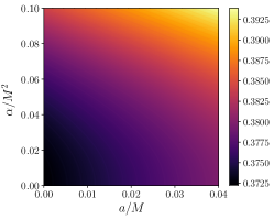
(a) $\textrm{Re}(\omega_{g}^{\textrm{axial}})$

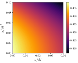
(b) $\textrm{Re}(\omega_{s})$

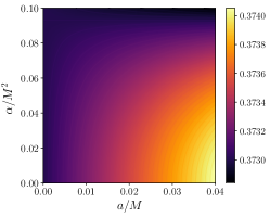
(c) $\textrm{Re}(\omega_{g}^{\textrm{polar}})$

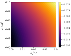
(d) $\textrm{Im}(\omega_{g}^{\textrm{axial}})$

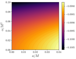
(e) $\textrm{Im}(\omega_{s})$

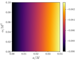
(f) $\textrm{Im}(\omega_{g}^{\textrm{polar}})$

Figure 5: Values of the QNM frequencies as functions of dimensionless spin ($a/M$) and CS coupling ($\alpha/M^{2}$) relative to their GR values as calculated with Eq. (56). Top row: from the left-most to right-most panel we show the values of the real part of the axial gravitational-led, the scalar-led and polar gravitational-led modes. Bottom row: the same, but for the imaginary part.

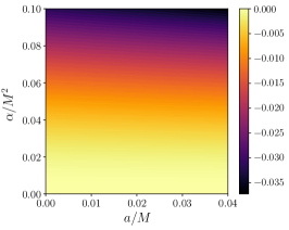
(a) $\delta\,\textrm{Re}(\omega_{g}^{\textrm{axial}})$

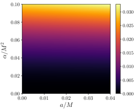
(b) $\delta\,\textrm{Re}(\omega_{s})$

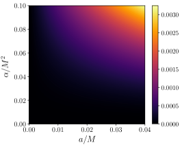
(c) $\delta\,\textrm{Re}(\omega_{g}^{\textrm{polar}})$

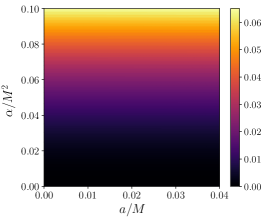
(d) $\delta\,\textrm{Im}(\omega_{g}^{\textrm{axial}})$

(e) $\delta\,\textrm{Im}(\omega_{s})$

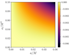
(f) $\delta\,\textrm{Im}(\omega_{g}^{\textrm{polar}})$

Figure 6: Fractional difference between the dCS QNM frequencies with respect to their GR values [calculated with Eq. (56)] as functions of dimensionless spin ($a/M$) and CS coupling ($\alpha/M^{2}$) parameters. Top row: from the left-most to right-most panel we show the fractional changes to the real part of the axial gravitational-led, the scalar-led and polar gravitational-led modes. Bottom row: the same, but for the imaginary part. In all cases, we see that the deviations become larger as we increase both $a/M$ and $\alpha/M^{2}$. For the range of these two parameters considered here, the largest deviation (of about $6\%$) occurs for the imaginary part of axial gravitational-led mode (bottom-left panel).

VI Discussion

We investigated the QNMs of slowly-rotating BHs in dCS gravity. We began by finding the perturbation equations that describe the evolution of scalar and tensorial perturbations. These triply-coupled set of ODEs generalize the slowly rotating versions of the Regge-Wheeler and the Zerilli-Moncrief master equations to the case of dCS gravity. Using symmetry arguments, we showed that not all terms in these equations contribute to the QNM frequencies, thus simplifying our set of equations into two sets: two coupled equations for the axial and the scalar sectors, and an homogeneous equation describing the polar sector; the latter was found to be independent of the coupling with the scalar field but included a CS modification to the effective potential thereby modifying the QNM frequencies.

We then solved these equations to calculate numerically the QNM frequencies. We found that the dCS corrections to the QNM frequencies scale with the square of the CS coupling. This was verified by means of a Fermi estimate as well as numerically. We also found that, in general, slowly-rotating BHs in dCS gravity have a decay time that is mostly independent of the CS coupling, so these BHs return to their stationary configuration on the same time-scale as in GR, but oscillating faster. Indeed, their (real) frequency of oscillation increases with the CS coupling at fixed spin-value for the axial gravitational-led modes, whereas it decreases for scalar-led modes while remaining effectively remaining almost constant (slightly decreasing) for polar gravitation-led modes. Finally, we constructed fitting functions for the real and imaginary parts of the gravitational and scalar QNM frequencies as a function of the BH mass, spin and CS coupling for the fundamental ($n=0$) mode and all $\ell\leqslant 4$ harmonics. We also found that the modes decay for all values of spin and CS coupling, a strong evidence that BHs described by Eq. (II.2) are stable against gravito-scalar perturbations, thus extending the results of Molina et al. (2010); Kimura (2018) to include spin. We have also verified our findings with those of Cano et al. (2020) who calculated the scalar QNM frequencies for a rotating BH solution in dCS gravity for a scalar field satisfying a homogeneous wave equation instead of Eq. (9).

What are the observational implications of our findings? Since GW detectors are capable of measuring only gravitational effects through GWs, the scalar modes of ringdown are not detectable with current technology. As a result, let us now focus only on the gravitational sector. Specifically in the axial gravitational sector, we find a degeneracy through a positive correlation between $a$ and $\alpha$ for the oscillatory frequencies; this is because the QNM frequency increases with increasing $a$ while keeping $\alpha$ constant and vice versa. This correlation is, however, found to break when considering the decay rates, because a change in the CS coupling barely affects the decay rate whereas a change in the spin parameter leads to longer lived modes. This result suggests that it may be possible to separate the effects of spin and the CS coupling for a loud enough ringdown observation.

The work presented here allows for many extensions along different directions. First, as it should be clear from our paper, we have here only considered perturbations to leading-order in the spin parameter. A natural extension of our work then would be to go to higher order in spin, which should produce more accurate results for BHs that are not as slowly spinning. Extending this calculation to second order, however, will be very difficult because of mode coupling between the odd- and even-parity sectors, just as in the GR case Pani et al. (2012a).

Another interesting extension of our work would be to develop a continued fraction approach for the calculation of the QNM frequencies in dCS gravity. Such a method was introduced by Leaver long ago, but its extension to modified gravity theories is not obvious Molina et al. (2010). One could therefore use dCS gravity as a toy problem to extend such methods, and then compare the results from the continued fraction method to the numerical results found in this paper. Additionally, this method can then be used in calculating the overtones for QNMs in dCS gravity, which is a limitation of the direct integration method used by us. Knowing the fundamental mode and at least one overtone, one can in principle constrain these modified theories of gravity using BH spectroscopy Isi and Farr (2021); Ota and Chirenti (2020, 2021).

The results that we presented in this paper can also serve as a way to verify numerical simulation of BH binaries that result in slowly-rotating BH remnants, such as the head-on collisions performed in Okounkova et al. (2019). A natural and important extension of our work, would be to extend the validity of our calculations to larger values of spin. Currently, the only way to find the QNM frequencies of not-slowly-spinning BHs in dCS is through numerical relativity simulations of BH mergers which are computationally expensive. Another interesting path for future research would then be to find a modified Teukolsky equation for dCS gravity. Such a task, however, may not be possible given that the BHs of dCS gravity are Petrov type I and not Petrov type D Yagi et al. (2012); Owen et al. (2021), as assumed in the work of Teukolsky Teukolsky (1973); Press and Teukolsky (1973).

Another interesting calculation would be to map our theory-specific numerical results to the theory-agnostic QNM parametrization introduced in Maselli et al. (2020) (see also Carullo (2021)). Our numerical results could also be used to quantify the error in theory-agnostic QNMs calculations due to the geometrical optics approximation, as done in Glampedakis et al. (2017); Glampedakis and Silva (2019); Silva and Glampedakis (2020). Yet another possible avenue for future work is to apply the tools developed here to study the oscillation spectra of rotating neutron stars in dCS gravity Yagi et al. (2013); Gupta et al. (2018). Such an analysis could have applications to GW asteroseismology Andersson and Kokkotas (1998); Pratten et al. (2020).

Finally, these results technically allow for the construction of ringdown templates that could be used by the LIGO-Virgo-Kagra collaboration to place constraints on dCS gravity. This would of course only be possible for ringdown signals produced by slowly-rotating BH remnants, which in turn only occurs when the inspiraling binary components have the right spin magnitude and orientation prior to merger. Whether the remnant is spinning or not, however, cannot currently be determined accurately enough because the signals detected so far do not have sufficiently high signal-to-noise ratio Colpi and Sesana (2017), and thus the posteriors on the spin are very wide Abbott et al. (2019, 2021). Moreover, such ringdown tests would require the unambiguous detection of more than one QNM mode Kokkotas and Schmidt (1999); Ota and Chirenti (2020); Jiménez Forteza et al. (2020) As the signal-to-noise ratio increases, it may be possible to carry out such a test, and in the meantime, it would be highly desirable to extend our results to more rapidly rotating BH backgrounds.

Appendix A Spherical Harmonics – orthogonality relations

In this appendix, we are providing some useful orthogonality relations for scalar, vector and tensor spherical harmonics. The scalar spherical harmonics satisfy a fundamental identity,

$$Y^{\ell m}_{,\theta\theta}+\cot\theta\,Y^{\ell m}_{,\theta}+\frac{1}{\sin^{2}\theta}Y^{\ell m}_{,\phi\phi}=-\ell(\ell+1)Y^{\ell m}\,.$$ (57)

They also satisfy the orthogonality relation given by

$$\langle Y^{\ell m},Y^{\ell^{\prime}m^{\prime}}\rangle=\delta^{\ell\ell^{\prime}}\delta^{mm^{\prime}}\,.$$ (58)

Vector spherical harmonics hold the following orthogonality relations,

$$\langle Y^{\ell m}_{a},Y^{\ell m}_{a}\rangle=\langle S^{\ell m}_{a},S^{\ell m}_{a}\rangle=(\ell-1)(\ell+2)+2\,,$$ (59)

where the polar and axial vector harmonics have been defined as

$$Y^{\ell m}_{a} =\left(Y^{\ell m}_{,\theta},Y^{\ell m}_{,\phi}\right)\,,$$

$$S^{\ell m}_{a} =\left(-\frac{Y^{\ell m}_{,\theta}}{\sin\theta},\sin\theta\,Y^{\ell m}_{,\theta}\right)\,.$$ (60)

Finally, the tensor spherical harmonics are given by

$$\langle Z^{\ell m}_{ab},Z^{\ell^{\prime}m^{\prime}}_{ab}\rangle =\langle S^{\ell m}_{ab},S^{\ell^{\prime}m^{\prime}}_{ab}\rangle$$

$$=2\ell(\ell-1)(\ell+1)(\ell+2)\delta^{\ell\ell^{\prime}}\delta^{mm^{\prime}}\,.$$ (61)

There are additional orthogonality relations which can be found in Pani (2013). The additional relations that we have used in this work are

$$\cos\theta\,Y^{\ell m}=q_{\ell+1,m}Y^{\ell+1,m}+ q_{\ell,m}Y^{\ell-1,m}\,,$$

$$\sin\theta\,Y^{\ell m}_{,\theta}=q_{\ell+1,m}\ell Y^{\ell+1,m}- q_{\ell,m}(\ell+1)Y^{\ell-1,m}$$

$$A_{\ell^{\prime}m^{\prime}}~{}\langle Y^{\ell m},\,\sin\theta\,Y^{\ell^{\prime}m^{\prime}}_{,\theta}\rangle =(\ell-1)q_{\ell m}A_{\ell-1,m}$$

$$-(\ell+2)q_{\ell+1,m} A_{\ell+1,m}\,,$$ (62)

where $q_{\ell m}$ is defined in Eq. (25). $A_{\ell m}$ is the operator defined to separate the angular dependence of the linearized field equations within the slow-rotation approximation.

Appendix B Coefficients of the perturbation equations

In this Appendix, we list the explicit forms of the coefficients appearing in the perturbation equations presented in Sec. III.2. These coefficients have prefactors of a combination of $\alpha,a$ and $m$ which have already been shown in the expression for the perturbation equations. However, it is worth noting that there is no direct correspondence between these coefficients. The potentials are given by:

$$V^{S}_{\rm eff} =\left(1-\frac{2M}{r}\right)\left[\frac{\ell(\ell+1)}{r^{2}}+\frac{2M}{r^{3}}\right]+2am\omega\left[\frac{4M}{r^{3}}-\alpha^{2}\frac{189M^{2}+120Mr+70r^{2}}{112\kappa r^{8}}\right]\,,$$ (63)

$$V^{A}_{\rm eff} =\left(1-\frac{2M}{r}\right)\left[\frac{\ell(\ell+1)}{r^{2}}-\frac{6M}{r^{3}}+\frac{am}{\omega}\frac{24M\left(3r-7M\right)}{\ell(\ell+1)r^{6}}\right]+2am\omega\left[\frac{4M}{r^{3}}\right.$$

$$\quad-\left.\alpha^{2}\frac{1}{112\kappa\lambda_{\ell}\ell(\ell+1)Mr^{13}\omega^{2}}\sum_{i=0}^{6}\Theta_{i}(r,\ell,\omega)M^{i}r^{6-i}\right]\,,$$ (64)

$$V^{P}_{\rm eff} =\left(1-\frac{2M}{r}\right)\left[\frac{2M}{r^{3}}+\frac{1}{3}\lambda_{\ell}\left(\frac{1}{r^{2}}+\frac{2\lambda_{\ell}(\ell^{2}+\ell+1)}{(6M+\lambda_{\ell}r)^{2}}\right)\right]$$

$$\quad+\frac{4amM}{r^{8}\ell(\ell+1)\left(\lambda_{\ell}r+6M\right)^{4}\omega}\left[\sum_{i=0}^{7}\xi_{i}(r,\ell,\omega)M^{i}r^{7-i}-\frac{\alpha^{2}}{448Mr^{5}\kappa}\sum_{i=0}^{10}\upsilon_{i}(r,\ell,\omega)M^{i}r^{10-i}\right]\,.$$ (65)

where $\lambda_{\ell}=(\ell+2)(\ell-1)$ and the functions $\xi_{i}$ are the same as those found for slowly rotating Kerr BHs in GR Pani (2013). We also provide all other functions in a Mathematica notebook that can be made available upon request. The other functions in the perturbed field equations that contribute to the QNM frequencies [See Eqs. (35)] are given by

$$g(r) =\frac{6i\lambda_{\ell}\ell(\ell+1)M}{r^{5}\omega}\,,$$ (66a)

$$h(r) =-\frac{i\left(r^{4}\omega^{2}\left(12(2\ell(\ell+1)-1)M^{2}+15Mr+5r^{2}\right)+144M^{3}(2M-r)\right)}{2Mr^{9}\omega^{2}}\,,$$ (66b)

$$j(r) =\frac{72iM^{2}(r-2M)}{r^{8}\omega^{2}}\,,$$ (66c)

and

$$v(r) =-\frac{6iM\omega}{\kappa r^{5}}\,,$$ (67a)

$$n(r) =\frac{i\left(-4224M^{4}+3306M^{3}r+48M^{2}r^{2}\left(r^{2}\omega^{2}-15\right)+5Mr^{3}+15r^{4}\right)}{4\kappa l(l+1)Mr^{9}}\,,$$ (67b)

$$p(r) =\frac{12iM(12M-5r)(2M-r)}{\kappa\ell(\ell+1)r^{8}}\,.$$ (67c)

All the other functions such as $k_{i},p_{i},s_{i}$ and $r_{i}$ ($i=1,\dots,4)$ are rather lengthy and non-illuminating and hence not provided here. Instead these can be found in a Mathematica notebook which can be made available upon request.

Appendix C QNM frequencies of different multipoles and fitting coefficients

In this appendix, we have tabulated the values of QNM frequencies for all multipoles of $\ell=2$ and $\ell=3$. $\ell=4$ values have been compiled into a data file available upon request. In the following tables, we have shown the values for the real and imaginary parts of the QNM frequencies for both gravitational- and scalar-led modes.

We then proceed to present the numerical values for the fitting functions shown in Eqs. (54) for both the gravitational and scalar QNM frequencies. We have also calculated the average percent error in these fits and presented these in our tables below.

Axial gravitational and scalar sectors

$a/M$	$\alpha/M^{2}$	$m=-2$	$m=-1$	$m=0$	$m=1$	$m=2$
	$0.0$	$.3737,.0889$	$.3737,.0889$	$.3737,.0889$	$.3737,.0889$	$.3737,.0889$
$0.0$	$0.05$	$.3757,.0879$	$.3757,.0879$	$.3757,.0879$	$.3757,.0879$	$.3756,.0879$
	$0.1$	$.3828,.0846$	$.3829,.0846$	$.3829,.0846$	$.3829,.0846$	$.3828,.0846$
	$0.0$	$.3723,.0881$	$.3729,.0887$	$.3737,.0889$	$.3743,.0887$	$.3749,.0881$
$0.01$	$0.05$	$.3744,.0872$	$.375,.0877$	$.3757,.0879$	$.3763,.0877$	$.3770,.0871$
	$0.1$	$.3816,.0839$	$.3822,.0844$	$.3829,.0846$	$.3836,.0844$	$.3845,.0839$
	$0.0$	$.3709,.0859$	$.3723,.0881$	$.3737,.0889$	$.3749,.0881$	$.3764,.0857$
$0.02$	$0.05$	$.373,.085$	$.3744,.0872$	$.3757,.0879$	$.377,.0871$	$.3786,.0849$
	$0.1$	$.3806,.0821$	$.3816,.0839$	$.3829,.0846$	$.3845,.0839$	$.3865,.0823$
	$0.0$	$.3693,.0829$	$.3716,.0871$	$.3737,.0889$	$.3756,.0870$	$.3783,.0825$
$0.03$	$0.05$	$.3716,.0822$	$.3737,.0862$	$.3829,.0846$	$.3778,.0862$	$.3806,.0819$
	$0.1$	$.3796,.0796$	$.3811,.0831$	$.3829,.0846$	$.3854,.0832$	$.3889,.0799$
	$0.0$	$.3678,.0796$	$.3709,.0859$	$.3737,.0889$	$.3764,.0857$	$.3805,.0792$
$0.04$	$0.05$	$.3702,.0791$	$.373,.085$	$.3671,.0926$	$.3786,.0849$	$.3829,.0788$
	$0.1$	$.3786,.0769$	$.3806,.0821$	$.3829,.0846$	$.3865,.0823$	$.3915,.0773$

Table 4: QNM frequencies for axial gravitational-led sector with $n=0,\,\ell=2$ for slowly rotating BHs in dCS gravity. The format used is $M$($\textrm{Re}(\omega),-\textrm{Im}(\omega)$). To save space, the leading zeros have been omitted.

$a/M$	$\alpha/M^{2}$	$m=-2$	$m=-1$	$m=0$	$m=1$	$m=2$
	$0.0$	$.4836,.0967$	$.4836,.0967$	$.4836,.0967$	$.4836,.0967$	$.4836,.0967$
$0.0$	$0.05$	$.4810,.0967$	$.4810,.0967$	$.4810,.0967$	$.4810,.0967$	$.4810,.0967$
	$0.1$	$.4720,.0970$	$.4720,.0970$	$.4720,.0970$	$.4720,.0970$	$.4720,.0970$
	$0.0$	$.4817,.0976$	$.4828,.0969$	$.4836,.0967$	$.4843,.0969$	$.4846,.0967$
$0.01$	$0.05$	$.4790,.0976$	$.4801,.0970$	$.4810,.0967$	$.4816,.097$	$.4819,.0976$
	$0.1$	$.470,.0979$	$.4711,.0973$	$.4720,.0970$	$.4726,.0972$	$.4729,.0979$
	$0.0$	$.4787,.1010$	$.4817,.0976$	$.4836,.0967$	$.4846,.0976$	$.4839,.1004$
$0.02$	$0.05$	$.4759,.1010$	$.4790,.0976$	$.4810,.0967$	$.4819,.0976$	$.4812,.1004$
	$0.1$	$.4667,.1012$	$.4701,.0979$	$.4720,.0970$	$.4729,.0979$	$.4718,.1008$
	$0.0$	$.4719,.1085$	$.4803,.0988$	$.4836,.0967$	$.4846,.0987$	$.4782,.1044$
$0.03$	$0.05$	$.4689,.1082$	$.4776,.0988$	$.4810,.0967$	$.4819,.0987$	$.4754,.1040$
	$0.1$	$.4577,.1082$	$.4686,.0992$	$.4720,.0970$	$.4727,.0991$	$.4652,.1038$
	$0.0$	$.4537,.107$	$.4787,.1007$	$.4836,.0967$	$.4840,.1004$	$.4692,.1005$
$0.04$	$0.05$	$.4512,.107$	$.4759,.1010$	$.4810,.0967$	$.4812,.1006$	$.4666,.1002$
	$0.1$	$.4424,.1049$	$.4667,.1012$	$.4720,.0970$	$.4718,.1008$	$.4573,.0994$

Table 5: Same as Table 4 but for the scalar-led sector with $n=0,\,\ell=2$.

$a/M$	$\alpha/M^{2}$	$m=-3$	$m=-2$	$m=-1$	$m=0$	$m=1$	$m=2$	$m=3$
	$0.0$	$.5994,.0927$	$.5994,.0927$	$.5994,.0927$	$.5994,.0927$	$.5994,.0927$	$.5994,.0927$	$.5994,.0927$
$0.0$	$0.05$	$.6078,.0911$	$.6078,.0911$	$.6078,.0911$	$.6078,.0911$	$.6078,.0911$	$.6078,.0911$	$.6078,.0911$
	$0.1$	$.6381,.1251$	$.6381,.1251$	$.6381,.1251$	$.6381,.1251$	$.6381,.1251$	$.6381,.1251$	$.6380,.1251$
	$0.0$	$.5970,.0911$	$.5979,.0919$	$.5987,.0925$	$.5994,.0927$	$.6001,.0925$	$.6007,.0919$	$.6013,.0911$
$0.01$	$0.05$	$.6055,.0896$	$.6063,.0904$	$.6069,.0909$	$.6078,.0911$	$.6085,.0909$	$.6092,.0904$	$.6100,.0895$
	$0.1$	$.6347,.1263$	$.6363,.1256$	$.6373,.1251$	$.6381,.1251$	$.6387,.1254$	$.6389,.1260$	$.6386,.1267$
	$0.0$	$.5941,.0874$	$.5961,.0900$	$.5979,.0919$	$.5994,.0927$	$.6007,.0919$	$.6019,.0899$	$.6035,.0871$
$0.02$	$0.05$	$.6032,.0859$	$.6048,.0885$	$.6063,.0904$	$.6092,.0904$	$.5799,.0955$	$.6108,.0884$	$.6128,.0858$
	$0.1$	$.6265,.1254$	$.6322,.1267$	$.6363,.1256$	$.6381,.1251$	$.6390,.1260$	$.6375,.1269$	$.6354,.1250$
	$0.0$	$.5912,.0829$	$.5942,.0874$	$.5971,.0911$	$.5994,.0927$	$.6013,.0911$	$.6034,.0871$	$.6064,.0825$
$0.03$	$0.05$	$.6008,.0816$	$.6032,.0859$	$.6055,.0896$	$.6078,.0911$	$.6100,.0895$	$.6128,.0858$	$.6162,.0816$
	$0.1$	$.6198,.1209$	$.6265,.1254$	$.6347,.1263$	$.6381,.1251$	$.6386,.1267$	$.6354,.1250$	$.6348,.1200$
	$0.0$	$.5883,.0787$	$.5922,.0844$	$.5961,.0900$	$.5994,.0927$	$.6019,.0899$	$.6053,.0841$	$.6099,.0782$
$0.04$	$0.05$	$.5984,.0775$	$.6016,.0829$	$.6048,.0885$	$.6078,.0911$	$.6108,.0884$	$.6150,.0830$	$.6202,.0777$
	$0.1$	$.6146,.1161$	$.6218,.1225$	$.6322,.1267$	$.6381,.1251$	$.6375,.1269$	$.6347,.1217$	$.6363,.1150$

Table 6: Same as Table 4 but for the axial gravitational-led sector with $n=0,\,\ell=3$.

$a/M$	$\alpha/M^{2}$	$m=-3$	$m=-2$	$m=-1$	$m=0$	$m=1$	$m=2$	$m=3$
	$0.0$	$.6753,.0965$	$.6753,.0965$	$.6753,.0965$	$.6753,.0965$	$.6753,.0965$	$.6753,.0965$	$.6753,.0965$
$0.0$	$0.05$	$.6656,.0969$	$.6656,.0969$	$.6656,.0969$	$.6656,.0969$	$.6656,.0969$	$.6656,.0969$	$.6656,.0969$
	$0.1$	$.6381,.1251$	$.6381,.1251$	$.6381,.1251$	$.6381,.1251$	$.6381,.1251$	$.6381,.1251$	$.6381,.1251$
	$0.0$	$.6714,.0974$	$.6731,.0969$	$.6744,.0966$	$.6753,.0965$	$.6759,.0966$	$.6761,.0968$	$.6758,.0971$
$0.01$	$0.05$	$.6616,.0979$	$.6634,.0973$	$.6647,.0970$	$.6656,.0969$	$.6661,.0973$	$.6662,.0973$	$.6658,.0976$
	$0.1$	$.6347,.1263$	$.6363,.1256$	$.6373,.1251$	$.6381,.1251$	$.6387,.1254$	$.6390,.1260$	$.6386,.1267$
	$0.0$	$.6630,.0989$	$.6693,.0979$	$.6731,.0969$	$.6753,.0965$	$.6761,.0968$	$.6750,.0974$	$.6720,.0969$
$0.02$	$0.05$	$.6525,.0994$	$.6593,.0985$	$.6634,.0973$	$.6656,.0969$	$.6662,.0973$	$.6648,.0979$	$.6614,.0971$
	$0.1$	$.6265,.1254$	$.6322,.1267$	$.6363,.1256$	$.6381,.1251$	$.6390,.1260$	$.6375,.1269$	$.6354,.1250$
	$0.0$	$.6515,.0961$	$.6630,.0989$	$.6715,.0973$	$.6753,.0965$	$.6758,.0972$	$.6720,.0969$	$.6679,.0919$
$0.03$	$0.05$	$.6411,.0959$	$.6526,.0994$	$.6616,.0979$	$.6656,.0969$	$.6658,.0976$	$.6614,.0971$	$.6572,.0917$
	$0.1$	$.6198,.1209$	$.6265,.1254$	$.6347,.1263$	$.6381,.1251$	$.6386,.1267$	$.6354,.1250$	$.6348,.1200$
	$0.0$	$.6428,.0903$	$.6551,.0976$	$.6693,.0979$	$.6753,.0965$	$.6750,.0974$	$.6689,.0939$	$.6671,.0855$
$0.04$	$0.05$	$.6326,.0902$	$.6446,.0976$	$.6593,.0985$	$.6656,.0969$	$.6648,.0979$	$.6582,.0938$	$.6563,.0852$
	$0.1$	$.6146,.1161$	$.6218,.1225$	$.6322,.1267$	$.6381,.1251$	$.6375,.1269$	$.6347,.1218$	$.6363,.1150$

Table 7: Same as Table 4 but for the scalar-led sector with $n=0,\,\ell=3$.

$m$	$f_{1}$	$f_{2}$	$f_{3}$	$f_{4}$	$f_{5}$	$f_{6}$	% error
$2$	$0.7814$	$9.4099$	$-0.4092$	$-8.2154$	$0.4546$	$3.5368$	$0.4$
$1$	$0.7156$	$4.0846$	$-0.3431$	$-2.8854$	$0.2028$	$5.2968$	$0.2$
$0$	$0.6864$	$0.60529$	$-0.3137$	$0.60431$	$\approx 0$	$\approx 0$	$0.02$
$-1$	$0.8109$	$-21.339$	$-0.4382$	$22.535$	$-0.2552$	$24.736$	$0.3$
$-2$	$0.8669$	$-24.001$	$-0.4942$	$25.188$	$-0.4277$	$34.662$	$0.3$

$m$	$f_{1}$	$f_{2}$	$f_{3}$	$f_{4}$	$f_{5}$	$f_{6}$	% error
$2$	$0.5454$	$-1.4771$	$-0.6360$	$2.0641$	$0.395$	$-1.2499$	$0.7$
$1$	$0.4953$	$-1.5226$	$-0.5854$	$2.1208$	$0.1549$	$-1.6087$	$0.5$
$0$	$0.4327$	$0.44203$	$-0.5222$	$0.15251$	$\approx 0$	$\approx 0$	$0.04$
$-1$	$0.4951$	$0.13356$	$-0.5851$	$0.46337$	$0.1453$	$-0.18332$	$0.6$
$-2$	$0.505$	$3.826$	$-0.5956$	$-3.2381$	$0.404$	$-1.4359$	$0.6$

Table 8: Same as Table 3 but for the axial gravitational-led sector and the $n=0,\,\ell=2$ mode for real (top) and imaginary (bottom) parts.

$m$	$g_{1}$	$g_{2}$	$g_{3}$	$g_{4}$	$g_{5}$	$g_{6}$	% error
$2$	$0.0358$	$-1.309$	$0.4527$	$-0.15518$	$0.875$	$5.1813$	$0.4$
$1$	$0.4108$	$-8.4164$	$0.07448$	$7.0422$	$0.267$	$8.7201$	$0.6$
$0$	$0.755$	$-1.3916$	$-0.2705$	$-0.014878$	$\approx 0$	$\approx 0$	$0.1$
$-1$	$0.2332$	$-5.1311$	$0.2517$	$3.7652$	$0.5398$	$4.8022$	$0.7$
$-2$	$0.09331$	$32.873$	$0.3645$	$-33.706$	$0.6074$	$7.751$	$0.4$

$m$	$g_{1}$	$g_{2}$	$g_{3}$	$g_{4}$	$g_{5}$	$g_{6}$	% error
$2$	$0.4943$	$-0.41208$	$-0.5929$	$0.20877$	$0.03482$	$-1.4985$	$1.6$
$1$	$0.4565$	$0.34382$	$-0.5519$	$-0.53517$	$-0.1934$	$-2.8791$	$1.5$
$0$	$0.5237$	$-0.66988$	$-0.6199$	$0.47395$	$\approx 0$	$\approx 0$	$0.2$
$-1$	$0.4395$	$-1.6133$	$-0.5347$	$1.4324$	$-0.2306$	$-6.1669$	$1.2$
$-2$	$0.6585$	$-13.538$	$-0.79$	$11.594$	$-0.5339$	$38.21$	$1.9$

Table 9: Same as Table 3 but for the scalar-led sector and the $n=0,\,\ell=2$ mode for real (top) and imaginary (bottom) parts.

$m$	$f_{1}$	$f_{2}$	$f_{3}$	$f_{4}$	$f_{5}$	$f_{6}$	% error
$3$	$1.233$	$-14.389$	$-0.6342$	$17.589$	$0.4971$	$-3.4131$	$0.2$
$2$	$1.058$	$-23.33$	$-0.4581$	$25.753$	$0.4438$	$-41.871$	$0.3$
$1$	$0.9376$	$-40.147$	$-0.339$	$44.144$	$0.2295$	$6.0011$	$0.1$
$0$	$0.8008$	$1.8508$	$-0.202$	$2.0534$	$\approx 0$	$\approx 0$	$0.1$
$-1$	$0.4219$	$-11.592$	$0.1769$	$15.583$	$0.4033$	$9.1724$	$0.05$
$-2$	$0.3243$	$-20.236$	$0.2745$	$24.276$	$0.5383$	$24.935$	$1.2$
$-3$	$0.2394$	$-19.856$	$0.3595$	$23.803$	$0.6471$	$29.555$	$1.6$

$m$	$f_{1}$	$f_{2}$	$f_{3}$	$f_{4}$	$f_{5}$	$f_{6}$	% error
$3$	$0.5702$	$3.2919$	$-0.6672$	$0.25096$	$0.5459$	$0.94723$	$3.9$
$2$	$0.5219$	$-8.7958$	$-0.6164$	$10.14$	$0.4255$	$-41.399$	$0.5$
$1$	$0.5218$	$-0.1413$	$-0.6106$	$-3.3617$	$0.1519$	$-19.551$	$3.5$
$0$	$0.4929$	$0.6282$	$-0.5811$	$-4.164$	$\approx 0$	$\approx 0$	$2.5$
$-1$	$0.5013$	$0.74239$	$-0.5901$	$-4.2191$	$0.1513$	$-19.53$	$4.5$
$-2$	$0.5151$	$-4.5501$	$-0.6043$	$0.9326$	$0.3959$	$-20.313$	$4.6$
$-3$	$0.5943$	$4.3365$	$-0.6836$	$-8.0688$	$0.5481$	$-17.372$	$4.2$

Table 10: Same as Table 3 but for the axial gravitational-led sector and the $n=0,\,\ell=3$ mode.

$m$	$g_{1}$	$g_{2}$	$g_{3}$	$g_{4}$	$g_{5}$	$g_{6}$	% error
$3$	$0.3327$	$47.358$	$0.3429$	$-51.198$	$0.7484$	$-75.948$	$0.3$
$2$	$0.2805$	$15.019$	$0.3965$	$-18.848$	$0.5196$	$-9.7528$	$0.2$
$1$	$0.5433$	$-3.161$	$0.1326$	$-0.54931$	$0.2796$	$1.0592$	$0.1$
$0$	$0.7772$	$5.2469$	$-0.102$	$-8.9636$	$-0.002274$	$0.2666$	$0.0$
$-1$	$0.3250$	$-2.8674$	$0.3509$	$-0.83273$	$0.508$	$-0.5176$	$0.1$
$-2$	$0.0359$	$6.9322$	$0.6421$	$-10.778$	$0.9033$	$-9.3872$	$0.2$
$-3$	$0.1106$	$-4.7023$	$0.5367$	$2.9615$	$0.842$	$6.626$	$3.0$

$m$	$g_{1}$	$g_{2}$	$g_{3}$	$g_{4}$	$g_{5}$	$g_{6}$	% error
$3$	$0.7327$	$-7.5698$	$-0.8297$	$4.5338$	$0.4339$	$-2.4478$	$3.5$
$2$	$0.4974$	$0.56638$	$-0.5926$	$-3.6759$	$0.2108$	$0.9019$	$3.1$
$1$	$0.4444$	$7.1089$	$-0.5377$	$-10.199$	$-0.03791$	$-1.074$	$2.8$
$0$	$0.5231$	$-0.92939$	$-0.6165$	$-2.1366$	$\approx 0$	$\approx 0$	$2.5$
$-1$	$0.4454$	$7.1024$	$-0.5385$	$-10.188$	$-0.08306$	$2.8145$	$2.7$
$-2$	$0.4852$	$-2.369$	$-0.5797$	$-0.76727$	$0.03384$	$15.112$	$2.8$
$-3$	$0.6379$	$-0.79127$	$-0.731$	$-2.4876$	$0.3901$	$1.2141$	$5.1$

Table 11: Same as Table 3 but for the scalar-led sector and the $n=0,\,\ell=3$ mode.

Polar gravitational sector

$a/M$	$\alpha/M^{2}$	$m=-2$	$m=-1$	$m=0$	$m=1$	$m=2$
	$0.0$	$.3737,.0889$	$.3737,.0889$	$.3737,.0889$	$.3737,.0889$	$.3737,.0889$
$0.0$	$0.05$	$.3737,.0889$	$.3737,.0889$	$.3737,.0889$	$.3737,.0889$	$.3737,.0889$
	$0.1$	$.3737,.0889$	$.3737,.0889$	$.3737,.0889$	$.3737,.0889$	$.3737,.0889$
	$0.0$	$.3726,.0881$	$.3730,.0888$	$.3737,.0889$	$.3744,.0888$	$.3751,.0882$
$0.01$	$0.05$	$.3726,.0881$	$.3730,.0888$	$.3737,.0889$	$.3744,.0888$	$.3751,.0882$
	$0.1$	$.3726,.0881$	$.3731,.0887$	$.3737,.0889$	$.3744,.0887$	$.3752,.0883$
	$0.0$	$.3712,.0861$	$.3725,.0882$	$.3737,.0889$	$.3751,.0882$	$.3768,.0859$
$0.02$	$0.05$	$.3712,.0861$	$.3725,.0882$	$.3737,.0889$	$.3751,.0882$	$.3768,.0859$
	$0.1$	$.3712,.0861$	$.3726,.0883$	$.3737,.0889$	$.3752,.0883$	$.3768,.0861$
	$0.0$	$.3699,.0832$	$.3719,.0872$	$.3737,.0889$	$.3759,.0873$	$.3789,.0829$
$0.03$	$0.05$	$.3699,.0832$	$.3719,.0874$	$.3737,.0889$	$.3759,.0873$	$.3789,.0829$
	$0.1$	$.3699,.0832$	$.3719,.0875$	$.3737,.0889$	$.3759,.0874$	$.3789,.0832$
	$0.0$	$.3682,.0801$	$.3711,.0862$	$.3737,.0889$	$.3767,.0859$	$.3811,.0799$
$0.04$	$0.05$	$.3682,.0805$	$.3713,.0861$	$.3737,.0889$	$.3810,.0801$	$.3829,.0788$
	$0.1$	$.3682,.0809$	$.3713,.0863$	$.3737,.0889$	$.3766,.0859$	$.3805,.0809$

Table 12: QNM frequencies for polar gravitational-led sector with $n=0,\,\ell=2$ for slowly rotating BHs in dCS gravity. The format used is $M$($\textrm{Re}(\omega),-\textrm{Im}(\omega)$). To save space, the leading zeros have been omitted.

$a/M$	$\alpha/M^{2}$	$m=-3$	$m=-2$	$m=-1$	$m=0$	$m=1$	$m=2$	$m=3$
	$0.0$	$.5994,.0927$	$.5994,.0927$	$.5994,.0927$	$.5994,.0927$	$.5994,.0927$	$.5994,.0927$	$.5994,.0927$
$0.0$	$0.05$	$.5994,.0927$	$.5994,.0927$	$.5994,.0927$	$.5994,.0927$	$.5994,.0927$	$.5994,.0927$	$.5994,.0927$
	$0.1$	$.5994,.0927$	$.5994,.0927$	$.5994,.0927$	$.5994,.0927$	$.5994,.0927$	$.5994,.0927$	$.5994,.0927$
	$0.0$	$.5972,.0911$	$.5980,.0920$	$.5987,.0925$	$.5994,.0927$	$.6001,.0925$	$.6008,.0919$	$.6014,.0911$
$0.01$	$0.05$	$.5972,.0912$	$.5980,.0920$	$.5988,.0925$	$.5994,.0927$	$.6001,.0925$	$.6008,.0920$	$.6014,.0911$
	$0.1$	$.5971,.0913$	$.5980,.0921$	$.5988,.0925$	$.5994,.0927$	$.6001,.0926$	$.6008,.0919$	$.6015,.0912$
	$0.0$	$.5947,.0874$	$.5963,.0901$	$.5980,.0919$	$.5994,.0927$	$.6008,.0919$	$.6022,.0899$	$.6038,.0872$
$0.02$	$0.05$	$.5947,.0875$	$.5963,.0901$	$.5980,.0919$	$.5994,.0927$	$.6008,.0920$	$.6022,.0900$	$.6038,.0872$
	$0.1$	$.5946,.0877$	$.5961,.0901$	$.5980,.0920$	$.5994,.0927$	$.6008,.0920$	$.6021,.0902$	$.6037,.0876$
	$0.0$	$.5917,.0831$	$.5945,.0874$	$.5972,.0911$	$.5994,.0927$	$.6015,.0911$	$.6038,.0872$	$.6069,.0827$
$0.03$	$0.05$	$.5915,.0832$	$.5945,.0875$	$.5972,.0912$	$.5994,.0927$	$.6015,.0911$	$.6038,.0873$	$.6068,.0828$
	$0.1$	$.5912,.0835$	$.5942,.0877$	$.5973,.0913$	$.5994,.0927$	$.6015,.0912$	$.6037,.0876$	$.6066,.0832$
	$0.0$	$.5888,.0787$	$.5927,.0845$	$.5964,.0901$	$.5994,.0927$	$.6022,.0899$	$.6047,.0869$	$.6103,.0785$
$0.04$	$0.05$	$.5987,.0790$	$.5925,.0846$	$.5964,.0901$	$.5994,.0927$	$.6022,.0900$	$.6045,.0869$	$.6102,.0787$
	$0.1$	$.5882,.0794$	$.5922,.0849$	$.5965,.0903$	$.5994,.0927$	$.6022,.0902$	$.6041,.0872$	$.6099,.0792$

Table 13: Same as Table 4 but for the polar gravitational-led sector with $n=0,\,\ell=3$.

$m$	$f_{1}$	$f_{3}$	$f_{5}$	$f_{6}$	% error
$2$	$0.9072$	$-0.5342$	$0.4833$	$-5.5714$	$0.1$
$1$	$0.7535$	$-0.3800$	$0.2582$	$-0.77801$	$0.1$
$0$	$0.6868$	$-0.3132$	$\approx 0$	$\approx 0$	$0.02$
$-1$	$0.6921$	$-0.3185$	$-0.1322$	$-0.3766$	$0.01$
$-2$	$0.7417$	$-0.3681$	$-0.2339$	$0.2931$	$0.01$

$m$	$f_{1}$	$f_{3}$	$f_{5}$	$f_{6}$	% error
$2$	$0.5117$	$-0.6017$	$0.3824$	$-2.171$	$0.7$
$1$	$0.5005$	$-0.5899$	$0.1328$	$0.1733$	$0.4$
$0$	$0.4351$	$-0.5239$	$\approx 0$	$\approx 0$	$0.02$
$-1$	$0.5001$	$-0.5895$	$0.1335$	$0.2283$	$0.4$
$-2$	$0.5158$	$-0.6058$	$0.3924$	$-2.0636$	$0.7$

Table 14: Same as Table 3 but for the polar gravitational-led sector and the $n=0,\,\ell=2$ mode for real (top) and imaginary (bottom) parts.

$m$	$f_{1}$	$f_{3}$	$f_{5}$	$f_{6}$	% error
$3$	$1.039$	$-0.4406$	$0.7068$	$-1.2427$	$0.1$
$2$	$1.048$	$-0.449$	$0.3923$	$-0.5770$	$0.1$
$1$	$0.8921$	$-0.2927$	$0.2417$	$-0.1956$	$0.1$
$0$	$0.7998$	$-0.2004$	$\approx 0$	$\approx 0$	$0.1$
$-1$	$0.413$	$0.1865$	$0.4049$	$-0.2653$	$0.1$
$-2$	$0.3065$	$0.2931$	$0.5563$	$-0.5452$	$0.1$
$-3$	$0.2187$	$0.381$	$0.6709$	$-0.7868$	$0.1$

$m$	$f_{1}$	$f_{3}$	$f_{5}$	$f_{6}$	% error
$3$	$0.6027$	$-0.6965$	$0.5076$	$1.8342$	$0.9$
$2$	$0.5094$	$-0.6032$	$0.3823$	$-2.1546$	$0.7$
$1$	$0.5022$	$-0.5953$	$0.1296$	$0.2921$	$0.3$
$0$	$0.5364$	$-0.6291$	$\approx 0$	$\approx 0$	$0.1$
$-1$	$0.4608$	$-0.5539$	$0.1397$	$-1.0851$	$0.3$
$-2$	$0.5074$	$-0.6012$	$0.375$	$-2.0335$	$0.7$
$-3$	$0.5912$	$-0.6851$	$0.5286$	$-0.7794$	$0.8$

Table 15: Same as Table 3 but for the polar gravitational-led sector and the $n=0,\,\ell=3$ mode.

References

- Will (2014) C. M. Will, “The confrontation between general relativity and experiment,” Living Reviews in Relativity 17, 4 (2014).
- Stairs (2003) I. H. Stairs, “Testing general relativity with pulsar timing,” Living Reviews in Relativity 6, 5 (2003).
- Wex and Kramer (2020) N. Wex and M. Kramer, “Gravity Tests with Radio Pulsars,” Universe 6, 156 (2020).
- Abbott et al. (2016) B. P. Abbott et al. (LIGO Scientific, Virgo), “Tests of general relativity with GW150914,” Phys. Rev. Lett. 116, 221101 (2016), [Erratum: Phys.Rev.Lett. 121, 129902 (2018)], arXiv:1602.03841 [gr-qc] .
- Yunes et al. (2016) N. Yunes, K. Yagi, and F. Pretorius, “Theoretical Physics Implications of the Binary Black-Hole Mergers GW150914 and GW151226,” Phys. Rev. D 94, 084002 (2016), arXiv:1603.08955 [gr-qc] .
- Yagi and Stein (2016) K. Yagi and L. C. Stein, “Black Hole Based Tests of General Relativity,” Class. Quant. Grav. 33, 054001 (2016), arXiv:1602.02413 [gr-qc] .
- Berti et al. (2018) E. Berti, K. Yagi, and N. Yunes, “Extreme Gravity Tests with Gravitational Waves from Compact Binary Coalescences: (I) Inspiral-Merger,” Gen. Rel. Grav. 50, 46 (2018), arXiv:1801.03208 [gr-qc] .
- Gnocchi et al. (2019) G. Gnocchi, A. Maselli, T. Abdelsalhin, N. Giacobbo, and M. Mapelli, “Bounding alternative theories of gravity with multiband GW observations,” Phys. Rev. D 100, 064024 (2019), arXiv:1905.13460 [gr-qc] .
- Toubiana et al. (2020) A. Toubiana, S. Marsat, S. Babak, E. Barausse, and J. Baker, “Tests of general relativity with stellar-mass black hole binaries observed by LISA,” Phys. Rev. D 101, 104038 (2020), arXiv:2004.03626 [gr-qc] .
- Perkins et al. (2021) S. E. Perkins, N. Yunes, and E. Berti, “Probing Fundamental Physics with Gravitational Waves: The Next Generation,” Phys. Rev. D 103, 044024 (2021), arXiv:2010.09010 [gr-qc] .
- Datta et al. (2021) S. Datta, A. Gupta, S. Kastha, K. G. Arun, and B. S. Sathyaprakash, “Tests of general relativity using multiband observations of intermediate mass binary black hole mergers,” Phys. Rev. D 103, 024036 (2021), arXiv:2006.12137 [gr-qc] .
- Gupta et al. (2020) A. Gupta, S. Datta, S. Kastha, S. Borhanian, K. G. Arun, and B. S. Sathyaprakash, “Multiparameter tests of general relativity using multiband gravitational-wave observations,” Phys. Rev. Lett. 125, 201101 (2020), arXiv:2005.09607 [gr-qc] .
- Perlmutter et al. (1999) S. Perlmutter et al. (Supernova Cosmology Project), “Measurements of and from 42 high redshift supernovae,” Astrophys. J. 517, 565–586 (1999), arXiv:astro-ph/9812133 .
- Riess et al. (1998) A. G. Riess et al. (Supernova Search Team), “Observational evidence from supernovae for an accelerating universe and a cosmological constant,” Astron. J. 116, 1009–1038 (1998), arXiv:astro-ph/9805201 .
- Sofue and Rubin (2001) Y. Sofue and V. Rubin, “Rotation curves of spiral galaxies,” Ann. Rev. Astron. Astrophys. 39, 137–174 (2001), arXiv:astro-ph/0010594 .
- Bertone and Hooper (2018) G. Bertone and D. Hooper, “History of dark matter,” Rev. Mod. Phys. 90, 045002 (2018), arXiv:1605.04909 [astro-ph.CO] .
- Canetti et al. (2012) L. Canetti, M. Drewes, and M. Shaposhnikov, “Matter and Antimatter in the Universe,” New J. Phys. 14, 095012 (2012), arXiv:1204.4186 [hep-ph] .
- Clifton et al. (2012) T. Clifton, P. G. Ferreira, A. Padilla, and C. Skordis, “Modified Gravity and Cosmology,” Phys. Rept. 513, 1–189 (2012), arXiv:1106.2476 [astro-ph.CO] .
- Berti et al. (2015) E. Berti et al., “Testing General Relativity with Present and Future Astrophysical Observations,” Class. Quant. Grav. 32, 243001 (2015), arXiv:1501.07274 [gr-qc] .
- Sotiriou (2006) T. P. Sotiriou, “f(R) gravity and scalar-tensor theory,” Class. Quant. Grav. 23, 5117–5128 (2006), arXiv:gr-qc/0604028 [gr-qc] .
- Kobayashi (2019) T. Kobayashi, “Horndeski theory and beyond: a review,” Rept. Prog. Phys. 82, 086901 (2019), arXiv:1901.07183 [gr-qc] .
- Skordis (2009) C. Skordis, “The Tensor-Vector-Scalar theory and its cosmology,” Class. Quant. Grav. 26, 143001 (2009), arXiv:0903.3602 [astro-ph.CO] .
- de Rham (2014) C. de Rham, “Massive Gravity,” Living Rev. Rel. 17, 7 (2014), arXiv:1401.4173 [hep-th] .
- Schmidt-May and von Strauss (2016) A. Schmidt-May and M. von Strauss, “Recent developments in bimetric theory,” J. Phys. A 49, 183001 (2016), arXiv:1512.00021 [hep-th] .
- Detweiler (1980) S. L. Detweiler, “Black holes and gravitational waves III. The resonant frequencies of rotating holes,” Astrophys. J. 239, 292–295 (1980).
- Dreyer et al. (2004) O. Dreyer, B. J. Kelly, B. Krishnan, L. S. Finn, D. Garrison, and R. Lopez-Aleman, “Black hole spectroscopy: Testing general relativity through gravitational wave observations,” Class. Quant. Grav. 21, 787–804 (2004), arXiv:gr-qc/0309007 .
- Berti et al. (2006) E. Berti, V. Cardoso, and C. M. Will, “On gravitational-wave spectroscopy of massive black holes with the space interferometer LISA,” Phys. Rev. D 73, 064030 (2006), arXiv:gr-qc/0512160 .
- Berti et al. (2007) E. Berti, J. Cardoso, V. Cardoso, and M. Cavaglia, “Matched-filtering and parameter estimation of ringdown waveforms,” Phys. Rev. D 76, 104044 (2007), arXiv:0707.1202 [gr-qc] .
- Sotiriou and Faraoni (2012) T. P. Sotiriou and V. Faraoni, “Black holes in scalar-tensor gravity,” Phys. Rev. Lett. 108, 081103 (2012), arXiv:1109.6324 [gr-qc] .
- Herdeiro and Radu (2015) C. A. R. Herdeiro and E. Radu, “Asymptotically flat black holes with scalar hair: a review,” Int. J. Mod. Phys. D 24, 1542014 (2015), arXiv:1504.08209 [gr-qc] .
- Motohashi and Minamitsuji (2018) H. Motohashi and M. Minamitsuji, “General Relativity solutions in modified gravity,” Phys. Lett. B 781, 728–734 (2018), arXiv:1804.01731 [gr-qc] .
- Barausse and Sotiriou (2008) E. Barausse and T. P. Sotiriou, “Perturbed Kerr Black Holes can probe deviations from General Relativity,” Phys. Rev. Lett. 101, 099001 (2008), arXiv:0803.3433 [gr-qc] .
- Yunes and Stein (2011) N. Yunes and L. C. Stein, “Non-Spinning Black Holes in Alternative Theories of Gravity,” Phys. Rev. D 83, 104002 (2011), arXiv:1101.2921 [gr-qc] .
- Yagi et al. (2016) K. Yagi, L. C. Stein, and N. Yunes, “Challenging the Presence of Scalar Charge and Dipolar Radiation in Binary Pulsars,” Phys. Rev. D 93, 024010 (2016), arXiv:1510.02152 [gr-qc] .
- Jackiw and Pi (2003) R. Jackiw and S. Y. Pi, “Chern-Simons modification of general relativity,” Phys. Rev. D 68, 104012 (2003), arXiv:gr-qc/0308071 [gr-qc] .
- Alexander and Gates (2006) S. H. S. Alexander and S. J. Gates, Jr., “Can the string scale be related to the cosmic baryon asymmetry?” JCAP 0606, 018 (2006), arXiv:hep-th/0409014 [hep-th] .
- Alexander and Yunes (2009) S. Alexander and N. Yunes, “Chern-Simons Modified General Relativity,” Phys. Rept. 480, 1–55 (2009), arXiv:0907.2562 [hep-th] .
- Nakamura et al. (2019) Y. Nakamura, D. Kikuchi, K. Yamada, H. Asada, and N. Yunes, “Weakly-gravitating objects in dynamical Chern–Simons gravity and constraints with gravity probe B,” Class. Quant. Grav. 36, 105006 (2019), arXiv:1810.13313 [gr-qc] .
- Yagi et al. (2013) K. Yagi, L. C. Stein, N. Yunes, and T. Tanaka, “Isolated and Binary Neutron Stars in Dynamical Chern-Simons Gravity,” Phys. Rev. D 87, 084058 (2013), [Erratum: Phys. Rev.D93,no.8,089909(2016)], arXiv:1302.1918 [gr-qc] .
- Nair et al. (2019) R. Nair, S. Perkins, H. O. Silva, and N. Yunes, “Fundamental Physics Implications for Higher-Curvature Theories from Binary Black Hole Signals in the LIGO-Virgo Catalog GWTC-1,” Phys. Rev. Lett. 123, 191101 (2019), arXiv:1905.00870 [gr-qc] .
- Silva et al. (2020) H. O. Silva, A. M. Holgado, A. Cárdenas-Avendaño, and N. Yunes, “Astrophysical and theoretical physics implications from multimessenger neutron star observations,” (2020), arXiv:2004.01253 [gr-qc] .
- Yunes and Sopuerta (2008) N. Yunes and C. F. Sopuerta, “Perturbations of Schwarzschild Black Holes in Chern-Simons Modified Gravity,” Phys. Rev. D 77, 064007 (2008), arXiv:0712.1028 [gr-qc] .
- Cardoso and Gualtieri (2009) V. Cardoso and L. Gualtieri, “Perturbations of Schwarzschild black holes in Dynamical Chern-Simons modified gravity,” Phys. Rev. D 80, 064008 (2009), [Erratum: Phys.Rev.D 81, 089903 (2010)], arXiv:0907.5008 [gr-qc] .
- Molina et al. (2010) C. Molina, P. Pani, V. Cardoso, and L. Gualtieri, “Gravitational signature of Schwarzschild black holes in dynamical Chern-Simons gravity,” Phys. Rev. D 81, 124021 (2010), arXiv:1004.4007 [gr-qc] .
- Kimura (2018) M. Kimura, “Stability analysis of Schwarzschild black holes in dynamical Chern-Simons gravity,” Phys. Rev. D 98, 024048 (2018), arXiv:1807.05029 [gr-qc] .
- Yunes and Pretorius (2009) N. Yunes and F. Pretorius, “Dynamical Chern-Simons Modified Gravity. I. Spinning Black Holes in the Slow-Rotation Approximation,” Phys. Rev. D 79, 084043 (2009), arXiv:0902.4669 [gr-qc] .
- Konno et al. (2009) K. Konno, T. Matsuyama, and S. Tanda, “Rotating black hole in extended Chern-Simons modified gravity,” Prog. Theor. Phys. 122, 561–568 (2009), arXiv:0902.4767 [gr-qc] .
- Pani (2013) P. Pani, “Advanced Methods in Black-Hole Perturbation Theory,” Int. J. Mod. Phys. A 28, 1340018 (2013), arXiv:1305.6759 [gr-qc] .
- Witek et al. (2019) H. Witek, L. Gualtieri, P. Pani, and T. P. Sotiriou, “Black holes and binary mergers in scalar Gauss-Bonnet gravity: scalar field dynamics,” Phys. Rev. D 99, 064035 (2019), arXiv:1810.05177 [gr-qc] .
- Okounkova et al. (2019) M. Okounkova, L. C. Stein, M. A. Scheel, and S. A. Teukolsky, “Numerical binary black hole collisions in dynamical Chern-Simons gravity,” Phys. Rev. D 100, 104026 (2019), arXiv:1906.08789 [gr-qc] .
- Maggiore (2018) M. Maggiore, Gravitational Waves. Vol. 2: Astrophysics and Cosmology (Oxford University Press, 2018).
- Misner et al. (1973) C. W. Misner, K. S. Thorne, and J. A. Wheeler, Gravitation (W. H. Freeman, San Francisco, 1973).
- Alexander et al. (2021) S. Alexander, G. Gabadadze, L. Jenks, and N. Yunes, “Chern-Simons caps for rotating black holes,” Phys. Rev. D 104, 064033 (2021), arXiv:2104.00019 [hep-th] .
- Delsate et al. (2015) T. Delsate, D. Hilditch, and H. Witek, “Initial value formulation of dynamical Chern-Simons gravity,” Phys. Rev. D 91, 024027 (2015), arXiv:1407.6727 [gr-qc] .
- Motohashi and Suyama (2011) H. Motohashi and T. Suyama, “Black hole perturbation in parity violating gravitational theories,” Phys. Rev. D 84, 084041 (2011), arXiv:1107.3705 [gr-qc] .
- Motohashi and Suyama (2012) H. Motohashi and T. Suyama, “Black hole perturbation in non-dynamical and dynamical Chern-Simons gravity,” Phys. Rev. D 85, 044054 (2012), arXiv:1110.6241 [gr-qc] .
- Yagi et al. (2012) K. Yagi, N. Yunes, and T. Tanaka, “Slowly Rotating Black Holes in Dynamical Chern-Simons Gravity: Deformation Quadratic in the Spin,” Phys. Rev. D 86, 044037 (2012), [Erratum: Phys.Rev.D 89, 049902 (2014)], arXiv:1206.6130 [gr-qc] .
- Maselli et al. (2017) A. Maselli, P. Pani, R. Cotesta, L. Gualtieri, V. Ferrari, and L. Stella, “Geodesic models of quasi-periodic-oscillations as probes of quadratic gravity,” Astrophys. J. 843, 25 (2017), arXiv:1703.01472 [astro-ph.HE] .
- Delsate et al. (2018) T. Delsate, C. Herdeiro, and E. Radu, “Non-perturbative spinning black holes in dynamical Chern–Simons gravity,” Phys. Lett. B 787, 8–15 (2018), arXiv:1806.06700 [gr-qc] .
- Regge and Wheeler (1957) T. Regge and J. A. Wheeler, “Stability of a schwarzschild singularity,” Phys. Rev. 108, 1063–1069 (1957).
- Sopuerta and Yunes (2009) C. F. Sopuerta and N. Yunes, “Extreme and Intermediate-Mass Ratio Inspirals in Dynamical Chern-Simons Modified Gravity,” Phys. Rev. D 80, 064006 (2009), arXiv:0904.4501 [gr-qc] .
- Wagle et al. (2019) P. Wagle, A. Saffer, and N. Yunes, “Polarization modes of gravitational waves in Quadratic Gravity,” Phys. Rev. D 100, 124007 (2019), arXiv:1910.04800 [gr-qc] .
- (63) https://github.com/pratikwagle/Quasinormal-modes-of-slowly-rotating-black-holes-in-dynamical-Chern-Simons-gravity.git.
- Chandrasekhar and Ferrari (1991) S. Chandrasekhar and V. Ferrari, “On the Non-Radial Oscillations of Slowly Rotating Stars Induced by the Lense-Thirring Effect,” Proceedings of the Royal Society of London Series A 433, 423–440 (1991).
- Pani et al. (2012a) P. Pani, V. Cardoso, L. Gualtieri, E. Berti, and A. Ishibashi, “Perturbations of slowly rotating black holes: massive vector fields in the Kerr metric,” Phys. Rev. D 86, 104017 (2012a), arXiv:1209.0773 [gr-qc] .
- Kojima (1993) Y. Kojima, “Coupled Pulsations between Polar and Axial Modes in a Slowly Rotating Relativistic Star,” Progress of Theoretical Physics 90, 977–990 (1993).
- Ferrari et al. (2007) V. Ferrari, L. Gualtieri, and S. Marassi, “A new approach to the study of quasi-normal modes of rotating stars,” Phys. Rev. D 76, 104033 (2007), arXiv:0709.2925 [gr-qc] .
- Pani et al. (2012b) P. Pani, V. Cardoso, L. Gualtieri, E. Berti, and A. Ishibashi, “Black hole bombs and photon mass bounds,” Phys. Rev. Lett. 109, 131102 (2012b), arXiv:1209.0465 [gr-qc] .
- Press (1971) W. H. Press, “Long Wave Trains of Gravitational Waves from a Vibrating Black Hole,” Astrophys. J. Lett. 170, L105–L108 (1971).
- Chandrasekhar and Detweiler (1975) S. Chandrasekhar and S. Detweiler, “The quasi-normal modes of the schwarzschild black hole,” Proceedings of the Royal Society of London. Series A, Mathematical and Physical Sciences 344, 441–452 (1975).
- Blázquez-Salcedo et al. (2016) J. L. Blázquez-Salcedo, C. F. B. Macedo, V. Cardoso, V. Ferrari, L. Gualtieri, F. S. Khoo, J. Kunz, and P. Pani, “Perturbed black holes in Einstein-dilaton-Gauss-Bonnet gravity: Stability, ringdown, and gravitational-wave emission,” Phys. Rev. D 94, 104024 (2016), arXiv:1609.01286 [gr-qc] .
- Leaver (1985) E. W. Leaver, “An analytic representation for the quasi normal modes of Kerr black holes,” Proc. Roy. Soc. Lond. A 402, 285–298 (1985).
- Maselli et al. (2020) A. Maselli, P. Pani, L. Gualtieri, and E. Berti, “Parametrized ringdown spin expansion coefficients: a data-analysis framework for black-hole spectroscopy with multiple events,” Phys. Rev. D 101, 024043 (2020), arXiv:1910.12893 [gr-qc] .
- Hatsuda and Kimura (2020) Y. Hatsuda and M. Kimura, “Semi-analytic expressions for quasinormal modes of slowly rotating Kerr black holes,” Phys. Rev. D 102, 044032 (2020), arXiv:2006.15496 [gr-qc] .
- Ayzenberg et al. (2016) D. Ayzenberg, K. Yagi, and N. Yunes, “Can the Slow-Rotation Approximation be used in Electromagnetic Observations of Black Holes?” Class. Quant. Grav. 33, 105006 (2016), arXiv:1601.06088 [astro-ph.HE] .
- Brill et al. (1972) D. R. Brill, P. L. Chrzanowski, C. Martin Pereira, E. D. Fackerell, and J. R. Ipser, “Solution of the scalar wave equation in a Kerr background by separation of variables,” Phys. Rev. D 5, 1913–1915 (1972).
- Berti et al. (2009) E. Berti, V. Cardoso, and A. O. Starinets, “Quasinormal modes of black holes and black branes,” Class. Quant. Grav. 26, 163001 (2009), arXiv:0905.2975 [gr-qc] .
-
(78)
https://pages.jh.edu/eberti2/ringdown
https://centra.tecnico.ulisboa.pt/network/grit/files/ringdown. - Cano et al. (2020) P. A. Cano, K. Fransen, and T. Hertog, “Ringing of rotating black holes in higher-derivative gravity,” Phys. Rev. D 102, 044047 (2020), arXiv:2005.03671 [gr-qc] .
- Abbott et al. (2017) B. . P. . Abbott et al. (LIGO Scientific, Virgo), “GW170608: Observation of a 19-solar-mass Binary Black Hole Coalescence,” Astrophys. J. 851, L35 (2017), arXiv:1711.05578 [astro-ph.HE] .
- Isi and Farr (2021) M. Isi and W. M. Farr, “Analyzing black-hole ringdowns,” (2021), arXiv:2107.05609 [gr-qc] .
- Ota and Chirenti (2020) I. Ota and C. Chirenti, “Overtones or higher harmonics? Prospects for testing the no-hair theorem with gravitational wave detections,” Phys. Rev. D 101, 104005 (2020), arXiv:1911.00440 [gr-qc] .
- Ota and Chirenti (2021) I. Ota and C. Chirenti, “Black hole spectroscopy horizons for current and future gravitational wave detectors,” (2021), arXiv:2108.01774 [gr-qc] .
- Owen et al. (2021) C. B. Owen, N. Yunes, and H. Witek, “Petrov type, principal null directions, and Killing tensors of slowly rotating black holes in quadratic gravity,” Phys. Rev. D 103, 124057 (2021), arXiv:2103.15891 [gr-qc] .
- Teukolsky (1973) S. A. Teukolsky, “Perturbations of a rotating black hole. 1. Fundamental equations for gravitational electromagnetic and neutrino field perturbations,” Astrophys. J. 185, 635–647 (1973).
- Press and Teukolsky (1973) W. H. Press and S. A. Teukolsky, “Perturbations of a Rotating Black Hole. II. Dynamical Stability of the Kerr Metric,” Astrophys. J. 185, 649–674 (1973).
- Carullo (2021) G. Carullo, “Accelerating modified gravity detection from gravitational-wave observations using the Parametrized ringdown spin expansion coefficients formalism,” (2021), arXiv:2102.05939 [gr-qc] .
- Glampedakis et al. (2017) K. Glampedakis, G. Pappas, H. O. Silva, and E. Berti, “Post-Kerr black hole spectroscopy,” Phys. Rev. D 96, 064054 (2017), arXiv:1706.07658 [gr-qc] .
- Glampedakis and Silva (2019) K. Glampedakis and H. O. Silva, “Eikonal quasinormal modes of black holes beyond General Relativity,” Phys. Rev. D 100, 044040 (2019), arXiv:1906.05455 [gr-qc] .
- Silva and Glampedakis (2020) H. O. Silva and K. Glampedakis, “Eikonal quasinormal modes of black holes beyond general relativity. II. Generalized scalar-tensor perturbations,” Phys. Rev. D 101, 044051 (2020), arXiv:1912.09286 [gr-qc] .
- Gupta et al. (2018) T. Gupta, B. Majumder, K. Yagi, and N. Yunes, “I-Love-Q Relations for Neutron Stars in dynamical Chern Simons Gravity,” Class. Quant. Grav. 35, 025009 (2018), arXiv:1710.07862 [gr-qc] .
- Andersson and Kokkotas (1998) N. Andersson and K. D. Kokkotas, “Towards gravitational wave asteroseismology,” Mon. Not. Roy. Astron. Soc. 299, 1059–1068 (1998), arXiv:gr-qc/9711088 .
- Pratten et al. (2020) G. Pratten, P. Schmidt, and T. Hinderer, “Gravitational-Wave Asteroseismology with Fundamental Modes from Compact Binary Inspirals,” Nature Commun. 11, 2553 (2020), arXiv:1905.00817 [gr-qc] .
- Colpi and Sesana (2017) M. Colpi and A. Sesana, “Gravitational Wave Sources in the Era of Multi-Band Gravitational Wave Astronomy,” in An Overview of Gravitational Waves: Theory, Sources and Detection, edited by G. Auger and E. Plagnol (2017) pp. 43–140, arXiv:1610.05309 [astro-ph.HE] .
- Abbott et al. (2019) B. P. Abbott et al. (LIGO Scientific, Virgo), “GWTC-1: A Gravitational-Wave Transient Catalog of Compact Binary Mergers Observed by LIGO and Virgo during the First and Second Observing Runs,” Phys. Rev. X 9, 031040 (2019), arXiv:1811.12907 [astro-ph.HE] .
- Abbott et al. (2021) R. Abbott et al. (LIGO Scientific, Virgo), “GWTC-2: Compact Binary Coalescences Observed by LIGO and Virgo During the First Half of the Third Observing Run,” Phys. Rev. X 11, 021053 (2021), arXiv:2010.14527 [gr-qc] .
- Kokkotas and Schmidt (1999) K. D. Kokkotas and B. G. Schmidt, “Quasinormal modes of stars and black holes,” Living Rev. Rel. 2, 2 (1999), arXiv:gr-qc/9909058 .
- Jiménez Forteza et al. (2020) X. Jiménez Forteza, S. Bhagwat, P. Pani, and V. Ferrari, “Spectroscopy of binary black hole ringdown using overtones and angular modes,” Phys. Rev. D 102, 044053 (2020), arXiv:2005.03260 [gr-qc] .
- (99) ““xAct: Efficient tensor computer algebra for the Wolfram Language”,” http://www.xact.es/.