Formation of black hole and accretion disk in a massive high-entropy stellar core collapse

Abstract

We present the first numerical result of fully general relativistic axisymmetric simulations for the collapse of a rotating high-entropy stellar core to a black hole and an accretion disk. The simulations are performed taking into account the relevant microphysics. We adopt as initial condition a spherical core with constant electron fraction ($Y_{e}=0.5$) and entropy per baryon $s$ = 8 $k_{B}$, and angular velocity is superimposed. In the early phase, the core collapses in a homologous manner. Then, it experiences a weak bounce due to the gas pressure of free nucleons. Because the bounce is weak, the core collapses eventually to a black hole. Subsequent evolution depends on initial angular velocity. When the rotation is not fast, a geometrically thin (but optically thick) accretion disk is formed, and shock waves are formed in the inner part of the disk. For the moderately rotating case, the thin accretion disk expands eventually to be a geometrically thick torus after sufficient accumulation of the thermal energy generated at the shocks. Furthermore, convection occurs inside the torus. Neutrino luminosities vary violently with time because of the convective motion. For the rapidly rotating case, by contrast, a geometrically thick torus is formed soon after the black hole formation, and convective activity is weak due to the presence of epicyclic mode.

1. Introduction

Gamma-ray bursts (GRBs) have been one of the most outstanding phenomena in the universe since their discovery in 1967 (Klebesadel et al., 1973) because of their huge energy emitted in a short timescale (isotopic equivalent luminosities of $10^{49}$–$10^{52}$ ergs/s in short duration of $\sim 0.01$–1000 s) and in addition, violent time variability of $\delta t\sim 1$ ms in time profiles of gamma-ray emission. GRBs are basically divided, in terms of their duration, into short bursts (SGRBs), for which duration is shorter than 2 s, and long bursts (LGRBs), for which duration is longer than 2 s. Recent observations have found GRBs with overlapped features of the two populations (Gehrels et al., 2006; Gal-Yam et al., 2006), and it is also suggested that a new classification may be necessary (Zhang et al., 2009; Lü et al., 2010). However, the large amount of energy release, short duration, and variability timescale indicate that GRBs may be universally associated with accretion processes onto a compact object of stellar-mass size (Piran, 1999). Because a rotating black hole is the most efficient converter of gravitational binding energy in nature, it is now widely believed that many of central engines of GRBs are composed of a rotating black hole surrounded by a massive and hot accretion disk.

Although progenitors of GRBs have not been fully clarified yet, there are accumulating observational evidences that LGRBs are associated with collapse of massive stars (Woosley & Bloom, 2006). (For reviews on progenitors of SGRBs, see e.g., Nakar (2007) and Lee & Ramirez-Ruiz (2007)). The first solid evidence for the connection between LGRBs and supernovae came from spectroscopic identification of a supernova component (SN2003dh) in the afterglow of GRB030329 (Hjorth et al., 2003; Stanek et al., 2003; Kawabata et al., 2003). To date, at least six other connections between LGRBs and supernovae have been reported: GRB980425 with SN1998bw (Galama et al., 1998; Kulkarni et al., 1998); XRF020903 (Soderberg et al., 2005); GRB021211 with SN2002lt (Della Valle et al., 2003) GRB031203 with SN2003lw (Malesani et al., 2004; Cobb et al., 2004; Thomsen et al., 2004; Gal-Yam et al., 2004); GRB050525a with SN2005nc (Della Valle et al., 2006b) and GRB060218 with SN2006aj (Campana et al., 2006; Pian et al., 2006; Mirabal et al., 2006; Modjaz et al., 2006; Sollerman et al., 2006); All the GRB-associated supernovae are TypeIb/c. In addition, there are a wide variety of circumstance evidences (Woosley & Bloom, 2006): E.g., observed association of afterglows of LGRBs with star forming regions in their host galaxies (Christensen et al., 2004; Fruchter et al., 2006; Savaglio et al., 2009; Svensson et al., 2010), and late time bumps resembled supernova components in light curves of LGRBs (Zeh et al., 2004, 2005, 2006).

The observational association between GRBs and supernovae has provided strong support to a scenario, so-called collapsar model, in which LGRBs are assumed to be originated in the collapse of a massive stellar core to a black hole (Woosley, 1993). MacFadyen & Woosley (1999) outlined possible scenarios of driving LGRBs. In the collapsar model, a central core of a massive star is required to be rotating rapidly enough that a massive accretion disk can be formed around a black hole. Then, pair annihilation of neutrinos emitted from the accretion disk to electron-positron pairs could supply sufficient energy to induce relativistic outflows (Eichler et al., 1989; Meszaros & Rees, 1992; Narayan et al., 1992; Mochkovitch et al., 1993). The relativistic outflows are expected to form a GRB fireball. In addition, it is suggested that strong magnetic fields of order $10^{15}$ G, if they are present, could play an active role in driving the relativistic outflows (Nakamura et al., 1992; Narayan et al., 1992; Lyuikov, 2006).

There are three possible varieties in collapsar model (Heger et al., 2003): In Type I (MacFadyen & Woosley, 1999) and Type II (MacFadyen et al., 2001) collapsar models, a proto-neutron star is assumed to be formed initially and a shock wave is launched. Then, in the Type I collapsar, the proto-neutron star collapses promptly to a black hole because the shock wave is weak, while in the Type II collapsar, a black hole is formed by a fallback process long after the proto-neutron star formation. In the Type III collapsar model (Heger et al., 2003; Fryer et al., 2001), a black hole is directly formed without formation of proto-neutron star.

Recently, two LGRBs (GRB060505 and GRB060614) which are not likely to be accompanied by a supernova were discovered (Fynbo et al., 2006; Gehrels et al., 2006; Gal-Yam et al., 2006; Della Valle et al., 2006a). The host galaxy of GRB0600505 is a star-forming galaxy similar to that of canonical LGRBs. Such LGRBs might be associated with the Type I or Type III collapsar. Note that there is debate about the lack of supernova feature in GRB06014 (Cobb et al., 2006; Dado et al., 2008) and it has been discussed that the duration of GRB060505 is about 4 second and it may be a short GRB (Ofek et al., 2007).

Because the observed supernovae associated with LGRBs are Type Ib/c and the relativistic jets have to reach the stellar surface (Zhang & Woosley, 2004), the progenitors should have lost their envelope before the onset of stellar core collapse; otherwise a peculiar evolution path is required. Due to these reasons, the progenitors of LGRBs are now believed to be rapidly rotating massive Wolf-Rayet (WR) stars. However, ordinary WR stars are known to be accompanied by strong stellar winds driven by radiation pressure which lead to a rapid spin-down of the stellar core. Here, a serious problem concerning collapsar model is that according to stellar evolution calculations, it is very difficult to produce pre-collapse cores which satisfy both the requirement of collapsar model and the association of Type Ib/c supernova, if magnetic torques and standard mass-loss rates are taken into account (Woosley & Heger, 2006).

To resolve the above dilemma, several models have been proposed (see Fryer et al. (2007) for a review). Izzard et al. (2004) and Podsiadlowski et al. (2004) proposed binary-interaction models, in which the tidal force in a close binary keeps a helium star in synchronous, rapid rotation. van den Heuvel & Yoon (2007) showed that a helium star in a close binary with a compact companion (i.e., neutron star or black hole) can retain sufficient angular momentum to form a progenitor of a GRB. Fryer & Heger (2005) suggested a binary-merger model and showed that a merger of two helium cores during the common-envelope inspiral phase can produce a rapidly rotating core which satisfies the requirement of the collapsar models.

On the other hand, Yoon & Langer (Yoon & Langer, 2005, 2006; Yoon et al., 2006) and Woosley & Heger (Woosley & Heger, 2006) recently showed that a single star can fulfill the requirements of the collapsar models if it is initially rapidly rotating ($\gtrsim 50$% of the Keplerian velocity at the equatorial surface) and of low metallicity ($Z/Z_{\odot}\lesssim 0.1$). Note that the low metallicity could keep the stellar radius smaller and also reduce the mass loss (Woosley & Heger, 2006). Both effects suppress the loss of angular momentum from the star. The rapid rotation results in a short mixing timescale, which could help achieving a chemically homogeneous state throughout the hydrogen burning phase. In this case, a single star could become a rapidly rotating WR star without losing the hydrogen envelope through the stellar wind, avoiding the red giant phase that otherwise would cause a significant decrease of the core angular momentum due to magnetic torques (Yoon & Langer, 2006). It is also noted that the chemically homogeneous evolution is likely to occur for the tidally spun-up star in a binary system (Cantiello et al., 2007).

There are several supports to the chemically-homogeneous-evolution model. Recent observations have indicated that LGRBs may prefer a low metallicity environment (Fruchter et al., 2006; Stanek et al., 2006; Modjaz et al., 2008; Svensson et al., 2010). If the binary merger model resulted in most of the LGRB progenitors, such dependency would not be found.

Gravitational collapse of population III (Pop III) stars, which are assumed to be formed from metal-free gas, may be accompanied by LGRB at a very high redshift (Schneider et al., 2002; Bromm & Loeb, 2006). Numerical simulations have suggested that Pop III stars would be predominantly very massive with $M\gtrsim 100M_{\odot}$ (Omukai & Para, 2001, 2003; Nakamura & Umemura, 2001; Abel et al., 2002; Bromm et al., 2002). Such a massive star may collapse directly to a black hole without producing supernova explosion (Type III collapsar).

In addition, an attempt to constrain the characteristics of LGRB progenitors has been made by Campana et al. (2008), who studied in detail an absorption pattern in the X-ray spectrum of GRB060218 and found an extremely low O/N ratio in the surrounding of the progenitor, reaching a conclusion that only a progenitor star characterized by a fast rotation and subsolar metallicity could explain it.

All of the above progenitor models of LGRBs are anomalous in the sense that they are different from the progenitors of ordinary supernovae. Qualitatively speaking, the progenitor models should produce a core of larger angular momentum than the ordinary supernova cores. Also, the central entropy of the core would be higher than the ordinary supernova cores because of its high mass: The chemically homogeneous models tend to predict a well-mixed, larger core with higher central entropy than the ordinary supernova core. It is also expected that the object formed after the binary merger will have a higher entropy, if the mass ratio of merging stars is not far from unity (Suzuki et al., 2007; Gaburov et al., 2008). Thus, LGRB progenitor cores may be modeled by a rapidly rotating, higher-entropy core, regardless of their formation processes. Based on this assumption, in this paper, we perform collapse simulations of a very massive stellar core with a fairly high value of entropy ($s=8k_{B}$ per baryon) to study effects of higher-entropy.

A number of hydrodynamic simulations have been performed for studying gravitational collapse of such rapidly rotating, higher-entropy core in the context of collapsar model: for the Type I collapsar model, see Proga et al. (2003), Fujimoto et al. (2006), Dessart et al. (2008), Nakataki (2009), Harikae et al. (2009), Lopez-Camara et al. (2009), and Ott et al. (2011); for the Type II collapsar model, see MacFadyen et al. (2001); for the Type III collapsar model, see Fryer et al. (2001), Shibata & Shapiro (2002), Sekiguchi & Shibata (2007), Suwa et al. (2007b), and Liu et al. (2007)). Most of the simulations were performed in the Newtonian or pseudo-Newtonian gravity (MacFadyen et al., 2001; Fryer et al., 2001; Proga et al., 2003; Fujimoto et al., 2006; Suwa et al., 2007b; Dessart et al., 2008; Harikae et al., 2009; Lopez-Camara et al., 2009). In such simulations, inner regions of core ($r\lesssim 5$–$20r_{\rm S}$ where $r_{\rm S}$ is the Schwarzschild radius) are excised, and consequently, increase of the overall efficiency of accretion according to the black hole spin from $\approx 6$% (zero spin) to $\approx 42$% (maximal spin) cannot be taken into account. The black hole spin has significant effects on structure of the accretion disk, because it dramatically changes the spacetime metric near the black hole, where most of accretion power is released (Chen & Beloborodov, 2007).

Also, to guarantee formation of a centrifugally supported accretion disk at radii larger than the excised radius, most of Newtonian studies adopted angular momentum distributions that are well above the threshold of the disk formation: The specific angular momentum $j$ for a large fraction of the core is assumed to be much larger than that at the innermost stable circular orbit (ISCO), $j_{\rm ISCO}$. In such cases, gravitational energy will not be effectively converted into thermal energy due to the large radii. Rather these models rely on subsequent hypothetical viscous heating for generating large amount of energy. By constant, Lee & Ramirez-Ruiz (2006) performed simulations of low angular momentum accretion flows into a black hole in the Newtonian framework. They found that a thin accretion disk is formed for $j\lesssim 1.9r_{\rm S}c$ while a thick torus is formed for $j\lesssim 2.1r_{\rm S}c$ (see also Lopez-Camara et al. (2009)). Harikae et al. (2009) also found similar results.

To self-consistently follow formation of a black hole and a surrounding disk, a fully general relativistic simulation for the collapse of rapidly rotating massive star was first performed by Shibata & Shapiro (2002). Unfortunately, they could not follow the subsequent evolution of an accretion disk around the black hole. Sekiguchi & Shibata (2007) and Liu et al. (2007) performed fully general relativistic simulations of collapsar, successfully following formation of an accretion disk and an early evolution of the disk. Recently, Ott et al. (2011) performed simulations in the context of the collapsar scenario and extracting the gravitational wave signature from it. Nakataki (2009) performed a long-term general relativistic simulation in a fixed Kerr black hole background. However, in these general relativistic simulations, relevant microphysical processes such as neutrino cooling were not taken into account.

In this paper, we for the first time report the results of fully general relativistic simulations for the collapse of a rapidly rotating, high-entropy core, taking into account detailed microphysics; a nuclear-theory-based finite-temperature equation of state (EOS), weak interaction processes such as electron capture and pair-neutrino processes, and neutrino cooling. We focus on self-consistently clarifying the formation process of a rotating black hole and surrounding accretion disk, and subsequent long-term evolution of this system. We will show how the black hole is formed and evolved, and also clarify the physical condition for the disk or torus in the vicinity of the black hole. In particular, this is the first work that clarifies the geometrical structure, thermal property (such as chemical composition, chemical potentials, and entropy), neutrino optical depth, and neutrino luminosities of the accretion disk in the framework of full general relativity.

The paper is organized as follows. We first briefly summarize the basic equations, the input physics, and numerical setup in Section 2. The main results are described in Section 3. Discussion of our results together with prospects for GRB production are given in Section 4. Section 5 is devoted to a summary. Throughout this paper, $\hbar$, $k_{B}$, $c$, and $G$ denote the Planck’s constant, the Boltzmann’s constant, the velocity of light, and the gravitational constant, respectively. We adopt the geometrical unit $c=G=1$ in Sections 2.1 and 2.2, which is commonly used in numerical relativity.

2. Setting

2.1. Einstein’s equation and gauge conditions

The standard variables in the 3+1 decomposition of Einstein’s equation are the three-dimensional metric $\gamma_{ij}$ and the extrinsic curvature $K_{ij}$ on the three-dimensional hypersurface defined by (York, 1979)

$$\gamma_{\mu\nu} \equiv g_{\mu\nu}+n_{\mu}n_{\nu},$$ (1)

$$K_{\mu\nu} \equiv -\frac{1}{2}\hbox{$\,{\cal L}\!\!\!$--}_{n}\gamma_{\mu\nu},$$ (2)

where $g_{\mu\nu}$ is the spacetime metric, $n_{\mu}$ is the unit normal to a three-dimensional hypersurface, and $\hbox{$\,{\cal L}\!\!\!$--}_{n}$ is the Lie derivative with respect to the unit normal $n^{\mu}$. Then we can write the line element in the form

$$ds^{2}=-\alpha^{2}dt^{2}+\gamma_{ij}(dx^{i}+\beta^{i}dt)(dx^{j}+\beta^{j}dt),$$ (3)

where $\alpha$ and $\beta^{i}$ are the lapse function and the shift vector which describe the gauge degree of freedom.

Numerical simulation is performed in the BSSN formulation (Shibata & Nakamura, 1995; Baumgarte & Shapiro, 1999) in which the spatial metric $\gamma_{ij}$ is conformally decomposed as $\gamma_{ij}=e^{4\phi}\tilde{\gamma}_{ij}$ where the condition $\det(\tilde{\gamma}_{ij})=1$ is imposed for the conformal metric $\tilde{\gamma}_{ij}$. From this condition, the conformal factor is written as $\phi=\frac{1}{12}\ln\gamma$ and $\gamma\equiv\det(\gamma_{ij})$. The extrinsic curvature $K_{ij}$ is decomposed into the trace part $K$ and the traceless part $A_{ij}$ as $K_{ij}=A_{ij}+(1/3)\gamma_{ij}K$ . The traceless part $A_{ij}$ is conformally decomposed as $A_{ij}=e^{4\phi}\tilde{A}_{ij}$. Consequently, the fundamental quantities for the evolution equation are now split into $\phi,\tilde{\gamma}_{ij}$, $K$, and $\tilde{A}_{ij}$. Furthermore, the auxiliary variable $F_{i}\equiv\delta^{jk}\partial_{k}\tilde{\gamma}_{ij}$ is introduced in the BSSN formulation (Shibata & Nakamura, 1995).

To stably follow the spacetime after appearance of a black hole, we evolve $W\equiv e^{-2\phi}$ instead of $\phi$ following Marronetti et al. (2008). The primary reason is that $\phi$ diverges at the center of a black hole in the vertex-center grid. With the choice of $W$, such pathology can be avoided, as first pointed out by Campanelli et al. (2006), in which $\chi\equiv e^{-4\phi}$ was used instead of $W$. Merits of using $W$ are that (i) the equation for the Ricci tensor is slightly simplified, (ii) no singular term appears in the evolution equations even for $W\rightarrow 0$, and (iii) the determinant of $\gamma_{ij}$ is always positive (Marronetti et al., 2008; Yamamoto et al., 2008).

We assume axial and equatorial symmetries of the spacetime and the so-called Cartoon method (Shibata, 2000, 2003a; Alcubierre et al., 2001) is adopted to avoid possible problems around the coordinate singularities of the cylindrical coordinates. In the present code, we use a 4th-order finite difference scheme in the spatial direction and a 3rd-order Runge-Kutta scheme in the time integration. The advection terms such as $\beta^{i}\partial_{i}\phi$ are evaluated by a 4th-order upwind scheme (Brügmann et al., 2008).

As the gauge conditions for the lapse, we use a dynamical slicing (cf. Alcubierre & Brügmann, 2001):

$$\partial_{t}\alpha=-2K\alpha.$$ (4)

It is known that this dynamical slicing enables to perform a long-term evolution of neutron stars as well as has a strong singularity avoidance property in the black hole spacetime. The shift vector is determined by solving the following dynamical equation (Shibata, 2003b)

$$\partial_{t}\beta^{k}=\tilde{\gamma}^{kl}(F_{l}+\Delta t\partial_{t}F_{l}).$$ (5)

Here the second term in the right-hand side is necessary for numerical stability, and $\Delta t$ denotes the numerical timestep.

2.2. Hydrodynamic equations coupled to general relativistic leakage scheme

Recently, Sekiguchi (2010a, b) developed a fully general relativistic hydrodynamic code implementing a nuclear-theory-based finite-temperature EOS, self-consistent electron and positron captures, and neutrino cooling by a general relativistic leakage scheme. Neutrino heating is not included in the current version of leakage scheme. Since we assume the axial and equatorial symmetry of the spacetime, the hydrodynamics equations are solved in the cylindrical coordinates $(\varpi,\varphi,z)$ where $\varpi=\sqrt{x^{2}+y^{2}}$. We follow Sekiguchi (2010b) for a solution of the hydrodynamic equations to which the readers may refer for the details. In this section, we adopt the geometrical unit $c=G=1$.

2.2.1 Energy-momentum conservation equation

The basic equations of general relativistic hydrodynamics with neutrinos are

$$\nabla_{\alpha}(T^{\rm Total})^{\alpha}_{\ \beta}=\nabla_{\alpha}\left[(T^{\rm F})^{\alpha}_{\ \beta}+(T^{\nu})^{\alpha}_{\ \beta}\right]=0,$$ (6)

where $(T^{\rm Total})_{\alpha\beta}$ is the total energy-momentum tensor, and $(T^{\rm F})_{\alpha\beta}$ and $(T^{\nu})_{\alpha\beta}$ are the energy-momentum tensor of fluids and neutrinos, respectively. Following Sekiguchi (2010b), the neutrino energy-momentum tensor is decomposed into ’trapped-neutrino’ ($(T^{\nu,{\rm T}})_{\alpha\beta}$) and ’streaming-neutrino’ ($(T^{\nu,{\rm S}})_{\alpha\beta}$) parts as

$$(T^{\nu})_{\alpha\beta}=(T^{\nu,{\rm T}})_{\alpha\beta}+(T^{\nu,{\rm S}})_{\alpha\beta}.$$ (7)

Here, the trapped-neutrino part phenomenologically represents neutrinos which interact sufficiently frequently with matter, and the streaming-neutrino part describes a phenomenological flow of neutrinos streaming out of the system. Liebendörfer et al. (2009) developed a more sophisticate method in terms of the distribution functions of trapped and streaming neutrinos in the Newtonian framework.

Streaming-neutrinos are produced with a leakage rate $Q^{\rm leak}_{\alpha}$, according to

$$\nabla_{\alpha}(T^{\nu,{\rm S}})^{\alpha}_{\ \beta}=Q^{\rm leak}_{\beta}.$$ (8)

On the other hand, the trapped-neutrino part is combined with the fluid part as

$$T_{\alpha\beta}\equiv(T^{\rm F})_{\alpha\beta}+(T^{\nu,{\rm T}})_{\alpha\beta}.$$ (9)

Then the equation for $T_{\alpha\beta}$ is

$$\nabla_{\alpha}T^{\alpha}_{\ \beta}=-Q^{\rm leak}_{\beta}.$$ (10)

We solve Eqs. (8) and (10) for the energy-momentum conservation equation.

The energy-momentum tensor of the fluid and trapped-neutrino parts ($T_{\alpha\beta}$) is treated as that of the perfect fluid,

$$T_{\alpha\beta}=(\rho+\rho\varepsilon+P)u_{\alpha}u_{\beta}+Pg_{\alpha\beta},$$ (11)

where $\rho$ and $u^{\alpha}$ are the rest mass density and the 4-velocity. The specific internal energy density ($\varepsilon$) and the pressure ($P$) are the sum of contributions from the baryons (free protons, free neutrons, $\alpha$-particles, and heavy nuclei), leptons (electrons, positrons, and trapped-neutrinos), and photons as,

$$P = P_{B}+P_{e}+P_{\nu}+P_{ph},$$ (12)

$$\varepsilon = \varepsilon_{B}+\varepsilon_{e}+\varepsilon_{\nu}+\varepsilon_{ph},$$ (13)

where subscripts ’$B$’, ’$e$’, ’$ph$’, and ’$\nu$’ denote the components of baryons, electrons and positrons, photons, and trapped-neutrinos, respectively.

The streaming-neutrino part, on the other hand, is set to be a general form of

$$(T^{\nu,{\rm S}})_{\alpha\beta}=En_{\alpha}n_{\beta}+F_{\alpha}n_{\beta}+F_{\beta}n_{\alpha}+P_{\alpha\beta},$$ (14)

where $F_{\alpha}n^{\alpha}=P_{\alpha\beta}n^{\alpha}=0$. In order to close the system, we need an explicit expression of $P_{\alpha\beta}$. In this paper, we adopt a simple form $P_{\alpha\beta}=\chi E\gamma_{\alpha\beta}$ with $\chi=1/3$. Then we solve Eq. (8) in a high resolution shock capturing scheme (Sekiguchi, 2010b).

The closure relation employed in this paper is not very physical. Also, recall that we do not consider the so-called neutrino heating in this paper. To treat the neutrino heating accurately, a more sophisticated closure relation is required. However, such a study is beyond the scope of this paper. A more sophisticated treatment of neutrino transport equations, together with incorporating the neutrino heating, will be needed in the future (e.g., Shibata et al., 2011).

2.2.2 Lepton-number conservation equations

The conservation equations of the lepton fractions are written schematically as

$$\!\!\frac{dY_{e}}{dt}=-\gamma_{e},$$ (15)

$$\!\!\frac{dY_{\nu_{e}}}{dt}=\gamma_{\nu_{e}},$$ (16)

$$\!\!\frac{dY_{\bar{\nu}_{e}}}{dt}=\gamma_{\bar{\nu}_{e}},$$ (17)

$$\!\!\frac{dY_{\nu_{x}}}{dt}=\gamma_{\nu_{x}},$$ (18)

where $Y_{e}$, $Y_{\nu_{e}}$, $Y_{\bar{\nu}_{e}}$, and $Y_{\nu_{x}}$ denote the fractions per baryon number for electrons, electron neutrinos, electron anti-neutrinos, and $\mu$ and $\tau$ neutrinos and anti-neutrinos, respectively. Here we consider, as local reactions, the electron capture, the positron capture, electron-positron pair annihilation, plasmon decay, and the Bremsstrahlung radiation of pair neutrinos, where $\nu$ and $\bar{\nu}$ denote the three flavors of neutrinos and anti-neutrinos.

The source terms are given by

$$\gamma_{e}=\gamma_{\nu_{e}}^{\rm local}-\gamma_{\bar{\nu}_{e}}^{\rm local},$$ (19)

$$\!\!\gamma_{\nu_{e}}=\gamma_{\nu_{e}}^{\rm local}-\gamma_{\nu_{e}}^{\rm leak},$$ (20)

$$\!\!\gamma_{\bar{\nu}_{e}}=\gamma_{\bar{\nu}_{e}}^{\rm local}-\gamma_{\bar{\nu}_{e}}^{\rm leak},$$ (21)

$$\!\!\gamma_{\nu_{x}}=\gamma_{\nu_{x}}^{\rm local}-\gamma_{\nu_{x}}^{\rm leak},$$ (22)

where $\gamma^{\rm local}$’s and $\gamma^{\rm leak}$’s are the local production and leakage rates of each species of neutrinos, respectively. Because $\gamma^{\rm local}_{\nu}$ ’s are characterized by the timescale of weak-interaction processes $t_{\rm wp}\sim|Y_{e}/\dot{Y}_{e}|$ which can be much shorter than the dynamical timescale (e.g., Bruenn, 1985), a straightforward explicit solution of Eqs. (15)–(18) leads, in general, to a numerical instability. Therefore we follow the procedure proposed in Sekiguchi (2010b) to solve the equations stably in an explicit manner.

First, in each timestep $n$, the conservation equation of the total lepton fraction ($Y_{l}=Y_{e}-Y_{\nu_{e}}+Y_{\bar{\nu}_{e}}$),

$$\!\!\frac{dY_{l}}{dt}=-\gamma_{l},$$ (23)

is solved together with the conservation equation of $Y_{\nu_{x}}$, Eq. (18), in advance of solving the whole of the lepton conservation equations (Eqs. (15) – (18)). Then, assuming that the $\beta$-equilibrium is achieved, values of the lepton fractions in the $\beta$-equilibrium ($Y_{e}^{\beta}$, $Y_{\nu_{e}}^{\beta}$, and $Y_{\bar{\nu}_{e}}^{\beta}$) are calculated from the evolved value of $Y_{l}$.

Second, regarding $Y_{\nu_{e}}^{\beta}$ and $Y_{\bar{\nu}_{e}}^{\beta}$ as the maximum allowed values of the neutrino fractions in the next timestep $n+1$, the source terms are limited so that each value of $Y_{\nu}$’s in the timestep $n+1$ cannot exceed that of $Y_{\nu}^{\beta}$ ’s. This limiter procedure enables to solve explicitly the whole of the lepton conservation equations (Eqs. (15) – (18)).

Third, the following conditions are checked,

$$\mu_{p}+\mu_{e}<\mu_{n}+\mu_{\nu_{e}},$$ (24)

$$\mu_{n}-\mu_{e}<\mu_{p}+\mu_{\bar{\nu}_{e}},$$ (25)

where $\mu_{p}$, $\mu_{n}$, $\mu_{e}$, $\mu_{\nu_{e}}$, and $\mu_{\bar{\nu}e}$ are the chemical potentials of protons, neutrons, electrons, electron neutrinos, and electron anti-neutrinos, respectively. If both conditions are satisfied, the values of the lepton fractions in the timestep $n+1$ are set to be those in the $\beta$-equilibrium value; $Y_{e}^{\beta}$, $Y_{\nu_{e}}^{\beta}$, and $Y_{\bar{\nu}_{e}}^{\beta}$. On the other hand, if either or both conditions are not satisfied, the lepton fractions in the timestep $n+1$ is set to be those obtained by solving the whole of the lepton-number conservation equations.

2.3. Microphysics

2.3.1 Equation of state

In this paper, we employ a tabulated EOS derived by Shen et al. (1998), which is based on the Brückner-Hartree-Fock-type relativistic mean field theory. The maximum gravitational mass of a cold spherical neutron star in this EOS is much larger than the canonical neutron star mass $\approx 1.4M_{\odot}$ as $\approx 2.2M_{\odot}$ (Shen et al., 1998). The framework of the relativistic mean field theory is extended with the Thomas-Fermi spherical cell model approximation to describe not only the homogeneous matter but also an inhomogeneous one.

The thermodynamical quantities of dense matter at various sets of $(\rho,Y_{p},T)$ are calculated to construct the numerical data table for simulation. Here $Y_{p}$ is the total proton fraction per baryon number. The original table covers a range of density $10^{5.1}$–$10^{15.4}$ g/cm³, proton fraction $0.0$–$0.56$, and temperature $0$–$100$ MeV, which are required for supernova simulation. The original table has been extended to higher density (Sumiyoshi et al., 2007, 2008) and higher temperature (Nakazato et al., 2008) ranges of $10^{5.1}$–$10^{17}$ g/cm³ and $0$–$400$ MeV, which are required for following black hole formation (Sumiyoshi et al., 2006).

It should be noted that the causality is guaranteed to be satisfied in this framework, whereas the sound velocity sometimes exceeds the velocity of the light in the non-relativistic framework, e.g., in the EOS by Lattimer & Swesty (1991). This is one of the benefits of the relativistic EOS.

To consistently calculate the pressure and the internal energy of electrons and positrons, the charge neutrality condition $Y_{p}=Y_{e}$ should be solved to determine the electron chemical potential $\mu_{e}$ for each value of the baryon rest mass density $\rho$ and the temperature $T$ in the EOS table. Namely, it is required to solve the equation

$$n_{e}(\mu_{e},T)\equiv n_{-}-n_{+}=\frac{\rho Y_{e}}{m_{u}}$$ (26)

in terms of $\mu_{e}$ for given values of $\rho$, $T$, and $Y_{e}\ (=Y_{p})$. Here, $m_{u}=931.49432$ MeV is the atomic mass unit, and $n_{-}$ and $n_{+}$ are the total number densities (i.e., including electron-positron pairs) of electrons and positrons, respectively. Then, assuming that electrons and positrons obey the Fermi-Dirac distribution, the number density, the pressure, and the internal energy density of electrons and positrons are calculated in a standard manner (e.g., Cox & Giuli, 1968).

The pressure and the specific internal energy density of photons are given by

$$P_{r}=\frac{a_{r}T^{4}}{3},\ \ \varepsilon_{r}=\frac{a_{r}T^{4}}{\rho},$$ (27)

where $a_{r}=(\pi^{2}k_{B}^{4})/(15c^{3}\hbar^{3})$ is the radiation constant.

In this paper, trapped-neutrinos are assumed to interact sufficiently frequently with matter that be thermalized. Therefore they are described as ideal Fermi gases with the matter temperature. From the numerically evolved neutrino fractions $Y_{\nu}^{\rm evol}$, the chemical potentials of neutrinos ($\mu_{\nu}$) are calculated by solving

$$Y_{\nu}^{\rm evol}=Y_{\nu}(\mu_{\nu},T)=\frac{m_{u}}{\rho}n_{\nu}(\mu_{\nu},T).$$ (28)

Then the pressure and the internal energy of trapped-neutrinos are calculated in the same manner as for electrons, using $\mu_{\nu}$ and the matter temperature.

2.3.2 Weak interaction and leakage rate

Following Sekiguchi (2010b), the leakage rates are defined by

$$\!\!Q_{\nu}^{\rm leak}=(1-e^{-b\tau_{\nu}})Q_{\nu}^{\rm diff}+e^{-b\tau_{\nu}}Q_{\nu}^{\rm local},$$ (29)

$$\!\!\gamma_{\nu}^{\rm leak}=(1-e^{-b\tau_{\nu}})\gamma_{\nu}^{\rm diff}+e^{-b\tau_{\nu}}\gamma_{\nu}^{\rm local},$$ (30)

where $\tau_{\nu}$ is the optical depth of neutrinos and $b$ is a parameter which is typically set as $b^{-1}=2/3$. The optical depth can be computed from the cross sections following an often employed prescription (Ruffert et al., 1996; Rosswog & Liebendörfer, 2003): The optical depth is calculated by

$$\tau_{\nu}={\rm min}\left[\tau^{\varpi}_{\nu},\tau^{z}_{\nu},\tau^{r}_{\nu}\right],$$ (31)

where $\tau_{\nu}^{\varpi}$, $\tau_{\nu}^{z}$, and $\tau_{\nu}^{r}$ are the optical depths along $\varpi$, $z$, and the radial directions, respectively. We calculate, for example, $\tau_{\nu}^{z}$ by

$$\tau_{\nu}^{z}(\varpi,z)=\int_{z}^{z_{\rm out}}\kappa_{\nu}(\varpi,z^{\prime})dz^{\prime},$$ (32)

where $\kappa_{\nu}$ is the opacity and $z_{\rm out}$ denotes the outer boundary in the $z$-direction. $\tau_{\nu}^{\varpi}$ and $\tau_{\nu}^{r}$ are calculated in a similar manner.

Then, because $Q^{\rm leak}_{\nu}$ should be regarded as the emissivity of neutrinos measured in the fluid rest frame, $Q^{\rm leak}_{\alpha}$ is defined as (Shibata et al., 2007; Sekiguchi, 2010a, b)

$$Q^{\rm leak}_{\alpha}=Q^{\rm leak}_{\nu}u_{\alpha}.$$ (33)

As the local production reactions of neutrinos, we consider the electron and positron captures ($\gamma_{\nu_{e}}^{\rm ec}$ and $\gamma_{\bar{\nu}_{e}}^{\rm pc}$) following Fuller et al. (1985), the electron-positron pair annihilation ($\gamma_{\nu_{e}\bar{\nu}_{e}}^{\rm pair}$ for electron-type neutrinos and $\gamma_{\nu_{x}\bar{\nu}_{x}}^{\rm pair}$ for the other type) following Cooperstein et al. (1986), the plasmon decays ($\gamma_{\nu_{e}\bar{\nu}_{e}}^{\rm plas}$ and $\gamma_{\nu_{x}\bar{\nu}_{x}}^{\rm plas}$) following Ruffert et al. (1996), and the Bremsstrahlung processes ($\gamma_{\nu_{e}\bar{\nu}_{e}}^{\rm Brems}$ and $\gamma_{\nu_{x}\bar{\nu}_{x}}^{\rm Brems}$) following Burrows et al. (2006). Then, the local reaction rates for the neutrino fractions are

$$\gamma_{\nu_{e}}^{\rm local}=\gamma_{\nu_{e}}^{\rm ec}+\gamma_{\nu_{e}\bar{\nu}_{e}}^{\rm pair}+\gamma_{\nu_{e}\bar{\nu}_{e}}^{\rm plas}+\gamma_{\nu_{e}\bar{\nu}_{e}}^{\rm Brems},$$ (34)

$$\gamma_{\bar{\nu}_{e}}^{\rm local}=\gamma_{\bar{\nu}_{e}}^{\rm pc}+\gamma_{\nu_{e}\bar{\nu}_{e}}^{\rm pair}+\gamma_{\nu_{e}\bar{\nu}_{e}}^{\rm plas}+\gamma_{\nu_{e}\bar{\nu}_{e}}^{\rm Brems},$$ (35)

$$\gamma_{\nu_{x}}^{\rm local}=\gamma_{\nu_{x}\bar{\nu}_{x}}^{\rm pair}+\gamma_{\nu_{x}\bar{\nu}_{x}}^{\rm plas}+\gamma_{\nu_{x}\bar{\nu}_{x}}^{\rm Brems}.$$ (36)

Similarly, the local neutrino energy emission rate $Q_{\nu}^{\rm local}$ is given by

$$Q_{\nu}^{\rm local}=Q_{\nu_{e}}^{\rm ec}+Q_{\bar{\nu}_{e}}^{\rm pc} + 2\,(Q_{\nu_{e}\bar{\nu}_{e}}^{\rm pair}+Q_{\nu_{e}\bar{\nu}_{e}}^{\rm plas}+Q_{\nu_{e}\bar{\nu}_{e}}^{\rm Brems})$$ (37)

$$+ 4\,(Q_{\nu_{x}\bar{\nu}_{x}}^{\rm pair}+Q_{\nu_{x}\bar{\nu}_{x}}^{\rm plas}+Q_{\nu_{x}\bar{\nu}_{x}}^{\rm Brems})\ .$$

The explicit forms of the local rates in Eqs. (34)–(37) are found in Sekiguchi (2010b).

We follow the recent work by Rosswog & Liebendörfer (2003) for the diffusive neutrino emission rates $\gamma_{\nu}^{\rm diff}$ and $Q_{\nu}^{\rm diff}$ in Eqs. (29) and (30). The explicit forms of $\gamma_{\nu}^{\rm diff}$ and $Q_{\nu}^{\rm diff}$ are found in Sekiguchi (2010b).

2.4. Initial model

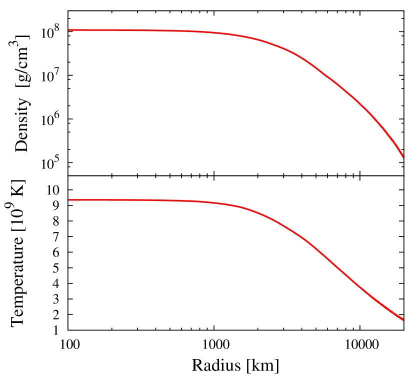
Figure 1.— Radial profiles of density (upper panel) and temperature (lower panel) of the initial configuration.

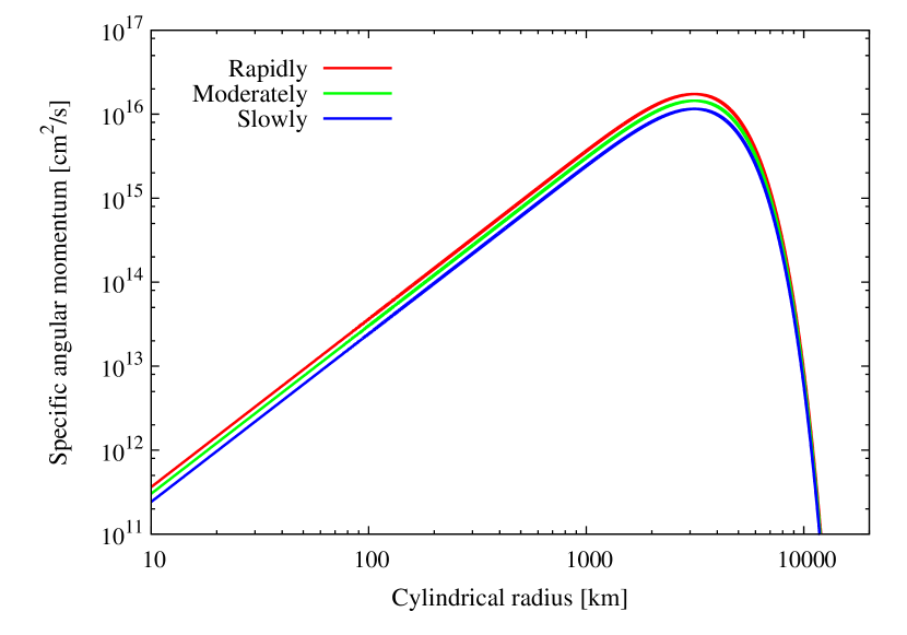
Figure 2.— Radial profiles of specific angular momentum for the slowly, moderately, and rapidly rotating models.

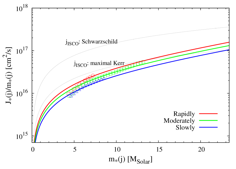
Figure 3.— Distributions of the averaged specific angular momentum for slowly (blue curve), moderately (green curve), and rapidly (red curve) rotating models. The specific angular momentum required to support a fluid element in a circular orbit at ISCO around a Schwarzschild black hole and a maximally rotating Kerr black hole of mass $m_{*}(j)$ is shown together (black dotted curves). The blue triangles, green squares, and red circles indicate the numerical results for the path along which specific angular momentum and mass of the black hole formed in the collapse of the slowly, moderately, and rapidly rotating models follow, respectively (see Sec. 3).

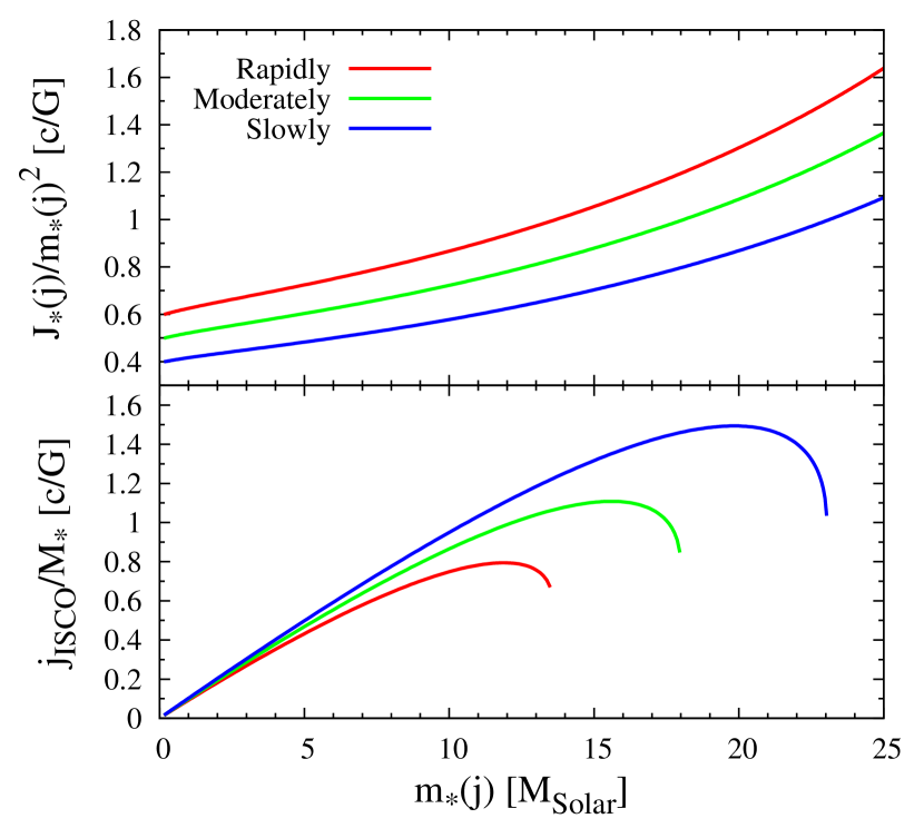
Figure 4.— The spin parameter distribution, $q_{*}(j)$, and the specific angular momentum at ISCO, $j_{\rm ISCO}(j)/M_{*}$, in units of $c/G$, where $M_{*}$ is the total baryon mass.

Because there are no realistic models of rotating progenitors derived by multi-dimensional pre-collapse evolution calculations or no binary progenitor models, we prepare approximate initial models in the following manner (Nakazato et al., 2007). We first calculate a spherical equilibrium configuration with a constant electron fraction of $Y_{e}=0.5$ and with a constant entropy per baryon $s=8k_{B}$. We set the central density to be $\rho_{c}\approx 10^{8}$ g/cm³. The corresponding central temperature is $T_{c}\approx 9\times 10^{9}$ K, which is higher than the critical temperature for the photo-dissociation of heavy nuclei to occur. Following Nakazato et al. (2007), we define the outer boundary of the ’iron core’ to be where the temperature is $5\times 10^{9}$ K. Note that most of heavy nuclei in inner parts of this ’iron core’ in fact are already photo-dissociated. Then the mass and the radius of the core are $M_{\rm iron}\approx 13M_{\odot}$ and $r_{\rm iron}\approx 7000$ km. In numerical simulation we follow a region of $r_{\rm tot}\approx 14000$ km ($>r_{\rm iron}$) in which the total mass of $M_{\rm tot}\approx 23M_{\odot}$ is enclosed. The radial profiles of density and temperature are shown in Figure 1.

For the purpose of reference, we note that our initial model might correspond to entropy per baryon for a star with initial mass of $\approx$ 120–$130M_{\odot}$ (Bond et al., 1984). However, a recent study (Waldman, 2008) predicts that such massive stars will undergo a pulsational pair instability and considerable mass loss, resulting in hydrostatic degenerate iron cores of mass with $\sim 3M_{\odot}$, which is different from the initial model adopted in this paper. The 300 $M_{\odot}$ progenitor used by Fryer et al. (2001) has a central entropy of $\sim 8k_{B}$ per baryon. However such a very massive model does not form an iron core in hydrostatic fashion, but rather goes unstable much earlier burning phase. Note that these are results in a spherical single star with solar metallicity. Anomalous stars, such as stars in interacting binary and Pop III stars, might form such high-entropy cores (Nakazato et al., 2007).

Little is also known about the angular momentum distribution in the progenitor core. Thus, we employ the following rotation profile

$$\Omega(\varpi)=\Omega_{0}\exp\left[-\frac{1}{2}\frac{R_{c}^{2}}{(\varpi^{2}+R_{c}^{2})}\right]\exp\left[-\frac{\varpi^{2}}{R_{0}^{2}}\right],$$ (38)

where $\varpi=\sqrt{x^{2}+y^{2}}$, and $\Omega$, $R_{0}$, and $R_{c}$ are parameters which control the degree of differential rotation. The exponential cut-off factor is introduced by a practical reason for numerical simulation: if the specific angular momentum in the outer region of the core is too large, the matter escapes from the computational domain. However, the most part of the ’iron core’ is almost uniformly rotating. We fix the values of $R_{0}$ and $R_{c}$ as $R_{0}=r_{\rm tot}/5$ and $R_{c}=r_{\rm tot}/8$, respectively. We vary $\Omega_{0}$ as 0, 0.4, 0.5 and 0.6 rad/s (hereafter referred to as spherical, slowly rotating, moderately rotating, and rapidly rotating models). The rotation period in the central region is $\approx 10$–15 s. This is by one order of magnitude longer than the dynamical timescale $(G\rho_{c})^{-1/2}\sim 0.4$ s. Thus, the progenitor star is not assumed to be rapidly rotating. The profiles of specific angular momentum along the cylindrical radius are plotted in Figure 2.

Figure 3 plots an averaged specific angular momentum distribution defined by $J_{*}(j)/m_{*}(j)$. Here, $j$ is the specific angular momentum of a fluid element, which is a conserved quantity in axially symmetric spacetime in the absence of viscosity. $m_{\ast}(j)$ is a rest mass distribution as a function of $j$, which is the integrated baryon rest mass of fluid elements with the specific angular momentum less than $j$, defined by (Shibata & Shapiro, 2002)

$$m_{\ast}(j)\equiv 2\pi\int_{j^{\prime}<j}\rho_{\ast}r^{2}drd(\cos\theta).$$ (39)

Similarly, $J_{*}(j)$ is an angular momentum distribution defined by

$$J_{\ast}(j)\equiv 2\pi\int_{j^{\prime}<j}\rho_{\ast}j^{\prime}r^{2}drd(\cos\theta).$$ (40)

These conserved quantities are often used in general relativistic study to predict a possible outcome of the collapse (Shibata & Shapiro, 2002; Shapiro, 2004; Sekiguchi & Shibata, 2004).

It should be noted that the specific angular momentum considered in this paper is rather small for a large fraction of fluid elements, in the sense that it is smaller than the angular momentum required for a fluid element to stay outside the innermost stable circular orbit (ISCO), $j_{\rm ISCO}$, around a Schwarzschild black hole. In this sense, our model is ’sub-Keplerian’. This is by contrast with many of previous models in which the specific angular momentum of well above $j_{\rm ISCO}$ is usually imposed (e.g., MacFadyen & Woosley (1999), but see Lee & Ramirez-Ruiz (2006), Lopez-Camara et al. (2009), and Harikae et al. (2009)). In the present condition, the fluid elements of such small specific angular momentum form a black hole, while those of large specific angular momentum does a disk (torus).

Now, to infer the evolution of a black hole surrounded by accreting materials, let us consider ISCO around a hypothetical black hole located at the center. If the value of $j$ of a fluid element is smaller than that at the ISCO, $j_{\rm ISCO}$, for the hypothetically formed black hole, the fluid element will fall into the seed black hole eventually. The value of $j_{\rm ISCO}$ will change as the ambient fluid elements accrete into the black hole. If $j_{\rm ISCO}$ increases as a result of the accretion, more ambient fluid elements will fall into the black hole. On the other hand, if $j_{\rm ISCO}$ decreases during the accretion, the accretion into the black hole will be suppressed, and then, the black hole will approach to a quasi-stationary state with a small accretion rate.

To estimate the value of $j_{\rm ISCO}$, we assume that the spacetime metric can be instantaneously approximated by that of a Kerr spacetime of mass $m_{*}(j)$ and the non-dimensional spin parameter $q_{*}(j)\equiv cJ_{*}(j)/Gm_{*}(j)^{2}$. On these approximations, we may compute $j_{\rm ISCO}$ of a black hole (e.g., Shapiro & Teukolsky, 1983).

For all the models considered in this paper, $q_{*}(j)$ is smaller than unity for a fraction of fluid elements with small specific angular momentum. As a result of this fact, these fluid elements can form a black hole in the dynamical timescale. However, this will not be the case for the initial condition with $q_{*}(j)>1$ in an inner region. In this case, a black hole will not be formed directly because the Kerr space time with the spin parameter greater than unity contains a naked singularity. Instead, a rotating oblate object will be the outcome (Saijo & Hawke, 2009; Sekiguchi & Shibata, 2004). Such an oblate object will be unstable against nonaxisymmetric deformation, and then, angular momentum will be transported by the hydrodynamic torque from the inner region to the outer one. As a result of a sufficient amount of angular momentum transport, a black hole will be eventually formed (Zink et al., 2007). This suggests that the timescale for black hole formation may be determined by the timescale for the angular momentum transport. We do not consider this possibility in this paper.

Figure 4 plots the spin parameter distribution ($q_{*}(j)$) and $j_{\rm ISCO}(j)=j_{\rm ISCO}[m_{*}(j),q_{*}(j)]$ as functions of $m_{*}(j)$. This figure clearly indicates that the value of $j_{\rm ISCO}(j)$ takes the maximum at $m_{*}(j)\approx 12,16,$ and 20$M_{\odot}$ for the rapidly, moderately, and slowly rotating models, respectively. These values show a possible final value of black hole mass, which is smaller than the total mass of the system. This indicates that a certain fraction of the material with mass $>M_{\odot}$ will form a disk around the black hole. It should be noted that the curves of Figures 3 and 4 indicate the possible evolution path of the black hole only approximately. In determining $j_{\rm ISCO}$ as a function of $m_{*}(j)$, we assume that a fluid element of smaller value of $j$ falls into black hole earlier. However, this is not always the case in the dynamical evolution of the system, because the material in the outer region near the rotation axis has a small value of $j$ and falls into the black hole in a late time.

2.5. Analysis of black hole and accretion disk

The formation of a black hole is ascertained by finding apparent horizon (Shibata, 1997). Then, we calculate two geometrical quantities which possibly characterize mass of a black hole. One is an irreducible mass defined by

$$M_{\rm irr}=\frac{c^{2}}{G}\sqrt{\frac{A_{H}}{16\pi}},$$ (41)

where $A_{H}$ is the area of the apparent horizon. The other mass is associated with the circumference proper length along the equatorial surface $C_{e}$:

$$M_{ce}=\frac{c^{2}}{G}\frac{C_{e}}{4\pi}.$$ (42)

This should agree with the mass of a Kerr black hole in the stationary axisymmetric spacetime. Note that in the case of a Schwarzschild black hole $M_{\rm irr}=M_{ce}$.

We also estimate black hole mass using an approximate conservation law,

$$M_{\rm con}=M_{\rm ADM}-M_{*,r>r_{AH}},$$ (43)

where $M_{\rm ADM}$ is the ADM mass of the system and $M_{*,r>r_{\rm AH}}$ is the rest mass of baryons located outside the apparent horizon. It is suggested that $M_{ce}$ may be a good indicator of mass of a black hole even in the presence of a massive accretion disk (Shibata, 2007). As we shall see in Section 3, $M_{ce}$ and $M_{\rm con}$ agree approximately with each other, and thus, we use $M_{ce}$ as the black hole mass, namely,

$$M_{\rm BH}\equiv M_{ce}\approx M_{\rm con}.$$ (44)

The non-dimensional spin parameter $q$ of a Kerr black hole can be calculated from the ratio between polar and equatorial circumferential radii of event horizon, $C_{p}$ and $C_{e}$,

$$\frac{C_{p}}{C_{e}}=\frac{\sqrt{2\hat{r}_{+}}}{\pi}\int_{0}^{\pi/2}d\theta\sqrt{1-\frac{q^{2}}{2\hat{r}_{+}}\sin^{2}\theta},$$ (45)

where $\hat{r}_{+}=1+\sqrt{1-q^{2}}$. The definition of $M_{\rm irr}$ for a Kerr black hole,

$$\frac{M_{\rm irr}}{M_{\rm BH}}=\sqrt{\frac{1}{2}\left(1+\sqrt{1-q^{2}}\right)}$$ (46)

may be also used to estimate the black hole spin. However, by contrast with $M_{ce}$, $C_{p}/C_{e}$ and $M_{\rm irr}/M_{\rm BH}$ are not very good indicators of the black hole spin when a massive disk presents (Shibata, 2007). In the case of equilibrium configuration of a black hole surrounded by a massive disk, it was found that a spin parameter estimated by Eqs. (45) and (46) decreases with the increase of disk mass and with the decrease of the inner edge of a disk. Accordingly, a spin parameter estimated by Eqs. (45) and (46) may contain an error of $\Delta q\sim 0.1$ because a massive accretion disk falling into a black hole is formed in the present study.

We note that we approximately calculate $C_{p}$, $C_{e}$, $M_{\rm BH}$, and $M_{\rm irr}$ measuring the geometrical quantities of apparent horizon. The disagreement between the event horizon and the apparent horizon may be large if the spacetime is not stationary, e.g., during the mass accretion phase in which the black hole mass dynamically increases. This fact makes the reliability of these methods worse. It should be noted that the dynamical horizon formalism (e.g., Schnetter et al., 2006) could be used to obtain more reliable estimation for mass and angular momentum of a dynamical black hole.

Instead of using Eqs. (45) and (46), we estimate angular momentum of a black hole using the conservation law,

$$J_{\rm BH}\equiv J_{\rm con}=J_{\rm tot}-J_{r>r_{AH}}-\Delta J_{\nu},$$ (47)

where $J_{\rm tot}$ is the total angular momentum of the system, $J_{r>r_{\rm AH}}$ is the amount of angular momentum located outside the apparent horizon, and $\Delta J_{\nu}$ is the amount of angular momentum carried away by neutrinos. We here ignore a small contribution of $\Delta J_{\nu}$. Then, we adopt the quantity

$$q_{\rm BH}\equiv\frac{cJ_{\rm con}}{GM_{\rm BH}^{2}}$$ (48)

as an approximate indicator of the non-dimensional spin parameter of a black hole.

An accretion disk will be formed in the collapse of the rotating models. Because it is difficult to strictly define disk mass, we approximately estimate it by

$$M_{\rm disk}\equiv\int_{\rho>\rho_{\rm cut},\,r_{\rm AH}<r<r_{\rm cut}}\rho_{*}d^{3}x,$$ (49)

where $\rho_{\rm cut}$ is a cutoff density which characterizes density near the surface of the accretion disk, $r_{\rm AH}$ is radius of apparent horizon, and $r_{\rm cut}$ is a cutoff radius which characterize the size of the accretion disk. Although $M_{\rm disk}$ is no more than an approximate indicator, the disk mass may be estimated by $M_{\rm disk}$ in a reasonable accuracy: When $\rho_{\rm cut}$ is larger than the surface density, slight change of $\rho_{\rm cut}$ will result in large change of $M_{\rm disk}$. By contrast, in the case that $\rho_{\rm cut}$ is smaller than the surface density, $M_{\rm disk}$ will not change much even if $\rho_{\rm cut}$ is decreased to some extent, because density outside the disk is low. We choose $\rho_{\rm cut}$ so that $M_{\rm disk}$ is not largely affected by a small change in $\rho_{\rm cut}$ and typically set $\rho_{\rm cut}=10^{10}$ g/cm³.

In this paper, we basically consider two rates, mass accretion rate into a black hole ($\dot{M}_{\rm BH}$) and mass infalling rate onto an accretion disk ($\dot{M}_{\rm disk}$), which are associated with time evolution of $M_{\rm BH}$ and $M_{\rm disk}$, respectively. The total mass infalling rate onto the system of a black hole surrounded by an accretion rate is then approximately given by $\dot{M}=\dot{M}_{\rm BH}+\dot{M}_{\rm disk}$.

2.6. Grid Setting

Table 1Summary of the regridding procedure

	$\Phi_{c}\leq 0.0125$	$\leq\Phi_{c}\leq 0.025$	$\leq\Phi_{c}\leq 0.05$	$\leq\Phi_{c}\leq 0.1$	$\Phi_{c}\leq 0.2$	$\Phi_{c}\geq 0.2$
$\Delta x_{0}$ (km)	10.1	4.8	2.2	0.98	0.45	0.22
$\delta$	0.008	0.0075	0.007	0.0065	0.006	0.0065
$N$	316	412	524	652	796	960
$L$ (km)	14600	13300	11800	10100	8700	7700
$\Delta x_{0}$ (km)	5.8	2.5	1.1	0.47	0.22	0.097
$\delta$	0.0075	0.007	0.0065	0.006	0.0055	0.005
$N$	400	520	656	812	980	1200
$L$ (km)	14600	13300	11800	10100	8700	7700

In numerical simulations, we adopt a nonuniform grid, in which the grid spacing is increased according to the rule

$$dx_{j+1}=(1+\delta)dx_{j},\ \ \ \ dz_{l+1}=(1+\delta)dz_{l},$$ (50)

where $dx_{j}\equiv x_{j+1}-x_{j}$, $dz_{l}\equiv z_{l+1}-z_{l}$, and $\delta$ is a constant. In addition, a regridding technique (Shibata & Shapiro, 2002; Sekiguchi & Shibata, 2005) is adopted to assign a sufficiently large number of grid points inside the collapsing core, saving the CPU time efficiently. The regridding is carried out whenever the characteristic radius of the collapsing star decreases by a factor of 2–3. At each regridding, the minimum grid spacing is decreased by a factor of $\sim 2$ and the geometrical factor $\delta$ is changed slightly.

All the quantities on the new grid are calculated using the fifth-order Lagrange interpolation. However, for the fluid quantities such as $\rho$ and $h$, the fifth-order interpolation could fail because the interpolation may give negative values of $\rho$ and $h-1$. In such cases, we adopt the linear interpolation to calculate the quantities on the new grid, based on the prescription proposed by Yamamoto et al. (2008). In each regridding, we solve the Hamiltonian constraint equation numerically.

To avoid discarding a large amount of the matter in the outer region (i.e., for approximately keeping the location of outer boundary), we also increase the grid number at each regridding. For the regridding, we define a relativistic gravitational potential $\Phi_{c}\equiv 1-\alpha_{c}~{}(\Phi_{c}>0)$ where $\alpha_{c}$ is the central value of the lapse function. Because $\Phi_{c}$ is approximately proportional to $M/R$ where $M$ and $R$ are characteristic mass and radius of the core, $\Phi_{c}^{-1}$ can be used as a measure of the characteristic length scale of the stellar core for the regridding.

To check the convergence of results, a simulation in a finer grid resolution is also performed. Table 1 summarizes the regridding parameters ($N$ and $L$ are mesh number and computational domain) of each level of the regridding procedure for normal (upper) and higher (lower) resolutions.

3. Results

3.1. Spherical model

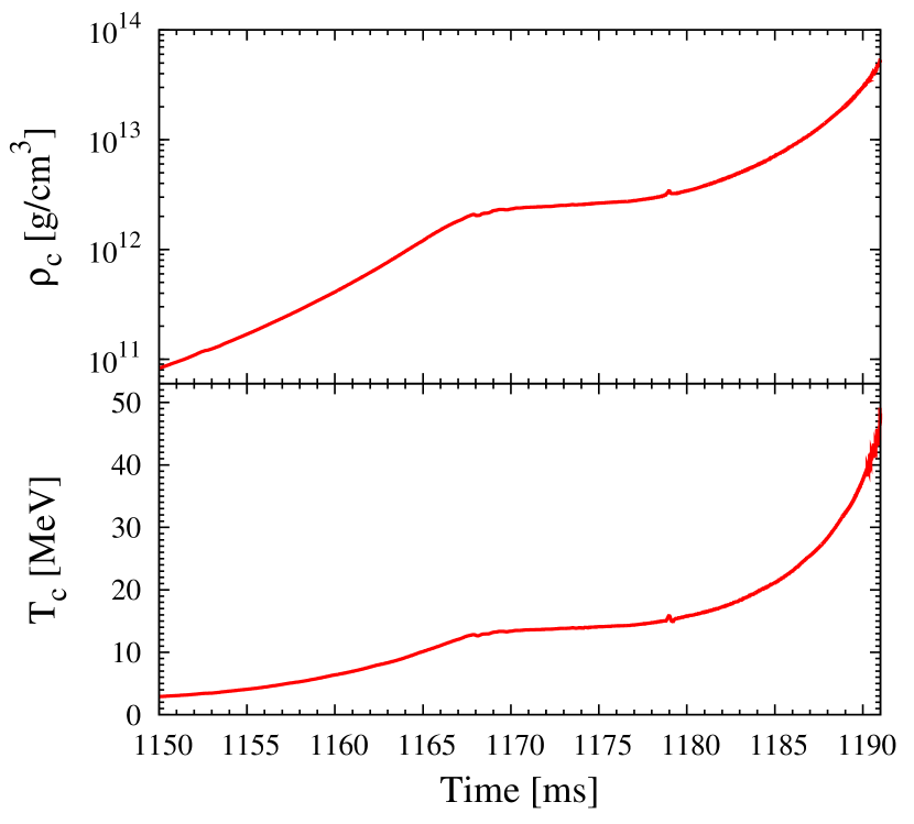
Figure 5.— Time evolution of the central values of density and temperature for the spherical model. The collapsing core experiences weak bounce at $t\approx 1168$ ms. We note that apparent horizon is formed at $t\approx 1193$ ms.

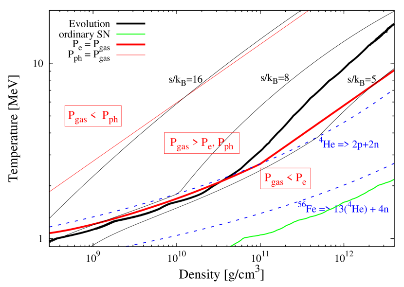
Figure 6.— Evolution path of the central values of density and temperature for the spherical model in $\rho$-$T$ plane (thick black solid curve). The thick and thin red solid curves show the boundary at which the condition $P_{e}=P_{\rm gas}$ or $P_{r}=P_{\rm gas}$ is satisfied. The thin black solid curves show evolution paths with constant entropy per baryon for $s/k_{B}=5$, 8 and 16. The two blue dashed curves denote the values of $(\rho,T)$ with which ⁵⁶Fe or ⁴He will be half by mass due to the photo-dissociation. An evolution path of the central values of density and temperature for an ordinary supernova core (Sekiguchi 2010b, see the text for details) is shown together (solid green curve).

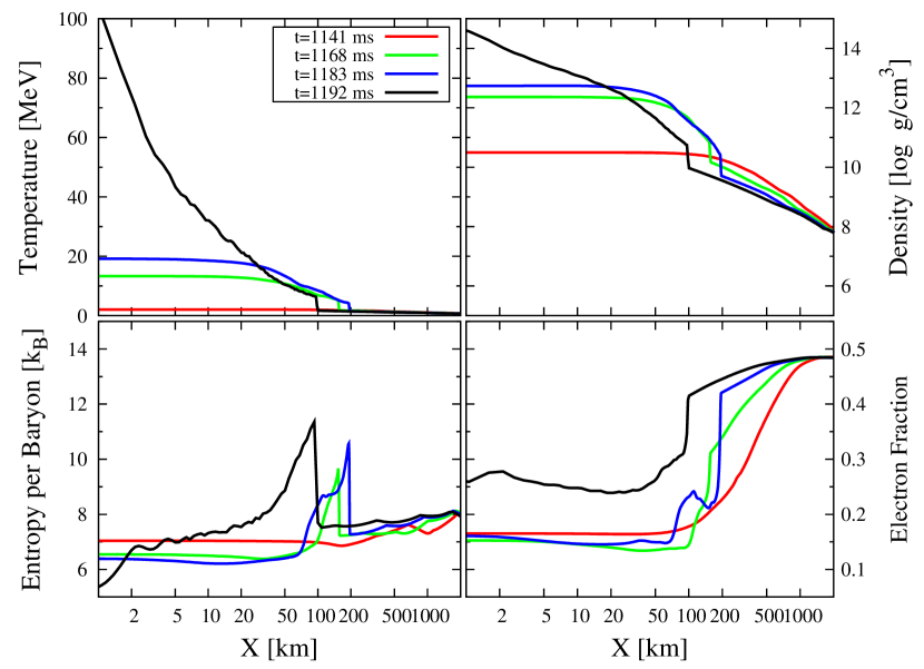
Figure 7.— Radial profiles of temperature, density, entropy per baryon, and electron fraction along the radial coordinate in the equator at $t\approx 1141$, 1168 (bounce), 1179 (shock stall), and 1192 (just before the apparent horizon formation) ms. Formation of a shock for $t\gtrsim 1168$ ms is due to the weak bounce.

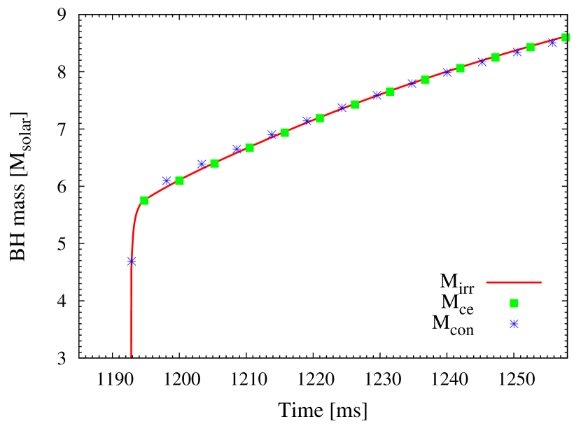
Figure 8.— Time evolution of black hole mass for the spherical model.

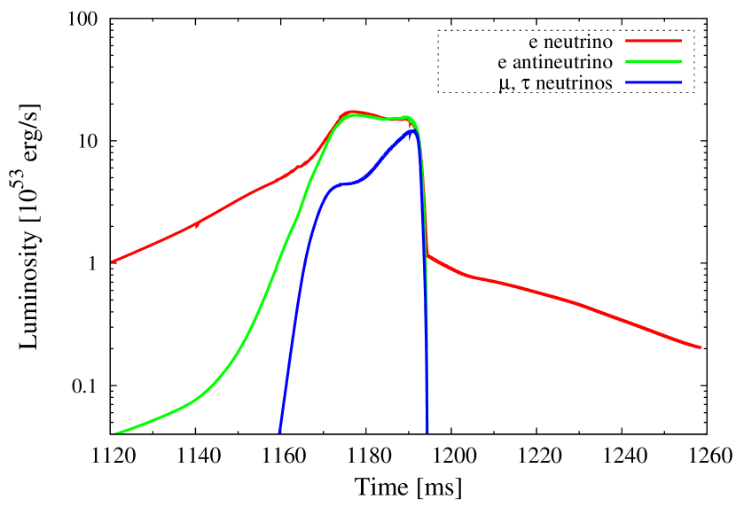
Figure 9.— Time evolution of neutrino luminosities for the spherical model. Note that the black hole is formed at $t\approx 1193$ ms.

In this section, we describe the features of collapse dynamics for the spherical model as a baseline for the rotational models described later. As in the core collapse of an ordinary supernova for which the central value of entropy per baryon is $s/k_{B}\sim 1$, gravitational collapse is triggered by the electron capture and the photo-dissociation of heavy nuclei. Then the collapse in the early phase proceeds in a homologous manner. Because of the higher value of the entropy per baryon ($s/k_{B}=8$), most of heavy nuclei are resolved into heliums by the photo-dissociation (cf. Figure 6). As the collapse proceeds and as a result, temperature increases, heliums are resolved into free nucleons ($p$, $n$). As we shall see below, due to the higher entropy and the resulting difference in the baryon composition, the collapse dynamics in a late phase is different from that of an ordinary supernova core.

3.1.1 Gas pressure dominated bounce

It is known that an ordinary supernova core experiences a bounce when the central density exceeds the nuclear density ($\rho_{\rm nuc}\sim 2\times 10^{14}$ g/cm³) above which the pressure increases drastically due to the repulsive nuclear force. In the present case, the collapse is not decelerated by the nuclear force but by the thermal gas pressure $P_{\rm gas}$ at a density far below $\rho_{\rm nuc}$. Such a feature of dynamics was already reported in the recent simulations (Fryer et al., 2001; Nakazato et al., 2007; Suwa et al., 2007b). We reconfirm this previous discovery and clarify the origin of this phenomena in more detail in the following.

The evolution of the central values of density and temperature for the spherical model is shown in Figure 5. At $t\approx 1168$ ms the core experiences a weak bounce (see also Figure 7). The central density at the bounce is below the nuclear density ($\approx 2\times 10^{12}$ g/cm³) and the central value of the temperature is $\approx 13$ MeV. At these values of central density and temperature, the pressure in the inner core is dominated by the thermal pressure of gas composed primarily of free nucleons and heliums.

This situation is different from that for $t\lesssim 1160$ ms, for which the pressure in most region of the inner part is dominated by the degenerate pressure of relativistic electrons. Because the adiabatic index of non-relativistic gas is $\Gamma=5/3$, which is much larger than that for relativistic degenerate electrons, $\Gamma\approx 4/3$, the collapse is decelerated due to a sudden increase of the pressure. The radial profiles of temperature, density, entropy, and entropy per baryon at the bounce along the equator are shown in Figure 7. This figure shows that the profiles do not vary significantly after the bounce, for $1168\lesssim t\lesssim 1183$ ms.

The critical value of entropy per baryon for the gas-pressure-dominated bounce to occur may be approximately estimated as follows. We plot paths along which entropy per baryon is constant in Figure 6 (see the thin black curves). For $s/k_{B}\lesssim 5$, paths of $P_{e}=P_{\rm gas}$ and constant entropy do not intersect. For $s/k_{B}\gtrsim 16$, on the other hand, the gas-pressure-dominated bounce cannot occur because the pressure is always dominated by the radiation pressure of photons (see the thin red curve in Figure 6). Therefore, most of the results obtained in this paper would be applied qualitatively to models with $5\lesssim s/k_{B}\lesssim 16$.

3.1.2 Shock stall and Black hole formation

As in the case of ordinary core collapse, a shock wave is formed at the gas-pressure-dominated bounce, and then, it propagates outward (see Figure 7). Because this bounce is weak, the shock wave is stalled soon after the bounce, at $t\approx 1179$ ms (cf. Figure 5). Near the stalled shock, a region of negative gradient of electron fraction ($\partial Y_{e}/\partial r<0$) is formed (see the blue curve in Figure 7) because neutrinos carry away the lepton number from the shock-heated region. It is known that such a configuration is unstable to convection. However, because the thermally supported hot inner core quickly ($\sim 10$ ms) collapses to a black hole, convection does not play an important role by contrast with the case of ordinary supernovae.

Figure 8 plots the time evolution of black hole mass for the spherical model. Note that the three masses of the black hole (see Section 2.5) approximately agree with each other (see Figure 8). Apparent horizon is formed at $t\approx 1193$ ms. After the apparent horizon formation, we continue the simulation using a hydrodynamic excision technique (Hawke et al., 2005), similar to adopted in Sekiguchi & Shibata (2007).

Black hole mass at the moment of its formation is $\approx 5.8M_{\odot}$, which is much larger than the maximum mass of cold spherical neutron stars ($M_{\rm coldNS,max}\approx 2.2M_{\odot}$ for Shen’s EOS). This is because the maximum mass of a hot neutron star can be much larger than the canonical value $M_{\rm coldNS,max}$ due to the higher entropy. It is found that approximate average value of the entropy is $s/k_{B}\sim 7$ just before the black hole formation (see Figure 7). Nakazato et al. (2007) calculated the maximum mass of a hot neutron star using Shen’s EOS. According to their result, the maximum mass is $\approx 5.6M_{\odot}$ for an isentropic core of $s/k_{B}\approx 7$ with $Y_{e}=0.1$, which agrees approximately with our present result. After the formation of the black hole, its mass increases gradually as the accretion of the material from the outer region proceeds. In the first $\sim 100$ ms, the mass accretion rate into the black hole is $\dot{M}_{\rm BH}\sim 30M_{\odot}$ s^-1.

3.1.3 Neutrino luminosities

Figure 9 plots the time evolution of neutrino luminosities for the spherical model. Before the weak bounce, average energy of $\mu$ and $\tau$ neutrinos is largest and electron neutrinos are dominantly emitted and emissivity of electron anti-neutrinos is much smaller because electrons are mildly degenerate with the electron degeneracy parameter of $\eta_{e}\sim 4(>1)$ and the positron fraction, responsible for anti-neutrino emission, is small. Note that the temperature is relatively low as $T\sim$ a few MeV. At leading order, ignoring the blocking terms due to weak degeneracy of neutrinos, energy emission rates associated with the electron capture and with the positron capture are, respectively, written as

$$Q^{\rm ec}_{\nu_{e}} \propto X_{p}F_{5}(\eta_{e}),$$ (51)

$$Q^{\rm pc}_{\bar{\nu}_{e}} \propto X_{n}F_{5}(-\eta_{e}).$$ (52)

Here, the Fermi-Dirac integrals are approximately given by (e.g., Fuller et al., 1985)

$$F_{5}(-\eta_{e}) \approx 120e^{-\eta_{e}},$$ (53)

$$F_{5}(\eta_{e}) \approx \frac{\eta_{e}^{6}}{6}+\frac{5\pi^{2}}{6}\eta_{e}^{4}+\frac{7\pi^{2}}{6}\eta_{e}^{2}+\frac{31\pi^{2}}{126}-120e^{-\eta_{e}},$$ (54)

which give, for $\eta_{e}\sim 4$, $F_{5}(\eta_{e})\sim 3000$ and $F_{5}(-\eta_{e})\sim 2$. For this stage, it is found $X_{p}/X_{n}\sim 0.1$ where $X_{n}$ and $X_{p}$ are the neutron and proton fractions. Therefore, the relation of $Q^{\rm ec}_{\nu_{e}}\gg Q^{\rm pc}_{\bar{\nu}_{e}}$ holds.

After the weak bounce, the degeneracy parameter becomes low as $\eta_{e}\sim 1.5$ because high temperature of $T\gtrsim 10$ MeV is achieved. In this case, $F_{5}(\eta_{e})\sim 300$ and $F_{5}(-\eta_{e})\sim 30$, and electron neutrinos and electron anti-neutrinos are approximately identically emitted for $X_{p}/X_{n}\sim 0.1$ because $Q^{\rm ec}_{\nu_{e}}\sim Q^{\rm pc}_{\bar{\nu}_{e}}$.

The peak luminosities of electron neutrinos ($\approx 1.8\times 10^{54}$ erg/s) and anti-neutrinos ($1.6\times 10^{54}$ erg/s) are achieved soon after the bounce (at $t\approx 1176$ ms) because neutrinos in the hot postshock region, where the density is not so large that optical depth for neutrinos is small, are copiously emitted. These luminosities remain approximately constant until black hole is formed. This happens due to the following competing effects; as a result of neutrino emission, thermal energy in the neutrino emission region is decreased, whereas as a result of compression associated with the collapse, temperature in the neutrino emission region is increased.

The peak luminosities of $\mu$ and $\tau$ neutrinos, on the other hand, are achieved just before the black hole formation. This is because the temperature significantly increases (see Figure 7) due to the adiabatic compression to enhance the pair production channel of neutrinos. Note that pair processes of neutrino production depend strongly on the temperature as $Q^{\rm pair}_{\nu\bar{\nu}}\propto T^{9}$. Just before the black hole formation, luminosities of all the species of neutrinos become approximately identical. This shows that the pair production process is dominant.

Soon after the black hole formation at $t\approx 1193$ ms, neutrino luminosities decrease drastically because the main neutrino-emission region is swallowed by the black hole. For the spherically symmetric case, i.e., in the absence of an accretion disk formation, neutrino luminosities damp monotonically as the density of infalling material decreases. The total energies emitted b neutrinos over the entire time of the simulation are $E_{\nu,{\rm tot}}\approx 8.3\times 10^{52}$, $5.2\times 10^{52}$, and $4.5\times 10^{52}$ erg for electron neutrinos, electron anti-neutrinos, and total of $\mu$ and $\tau$ neutrinos, respectively.

Before closing this subsection, we briefly compare our results for the spherical model with those in Nakazato et al. (2007), who performed spherically symmetric general relativistic simulations in which the Boltzmann equation is solved for neutrino transfer with relevant weak interaction processes. Note that the evolution after the black hole formation was not followed in their simulations because they adopted the so-called Misner-Sharp coordinates (Misner & Sharp, 1964), by which evolution of black hole cannot be followed. According to their results for a model with the initial entropy of $s/k_{B}=7.5$, the maximum neutrino luminosities achieved are $L_{\nu_{e}}\approx L_{\bar{\nu}_{e}}\approx 8\times 10^{53}$ erg/s and $L_{\nu_{x}}\approx 4\times 10^{53}$ erg/s, which are by a factor of 2–3 smaller than those in our results. The primary reason for this is that their computation was finished before the peak luminosity is reached due to the choice of their time coordinate, which is not suitable for following black hole evolution. However, the qualitative feature of luminosity curves for each species of neutrinos in our simulation agrees with that in Nakazato et al. (2007) for the phase before the black hole formation.

3.2. Moderately rotating model

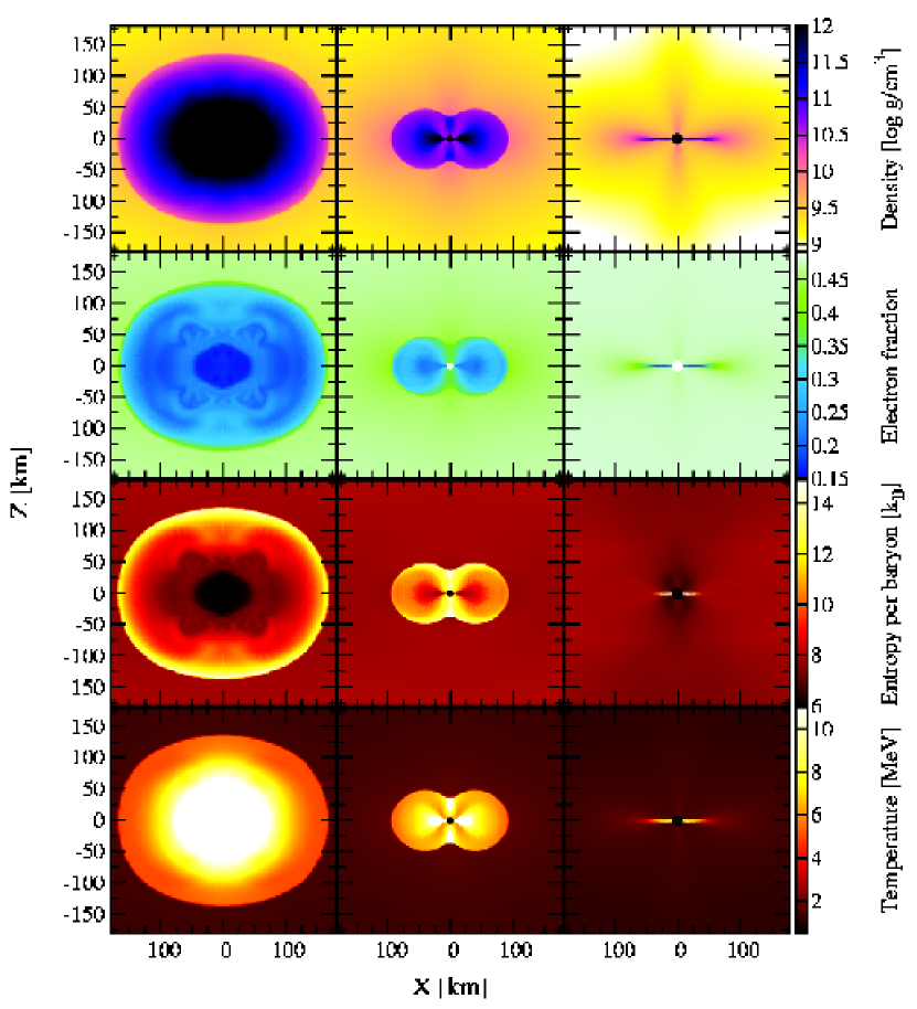
Figure 10.— Contours of rest mass density (panels in the first row), electron fraction (panels in the second row), entropy per baryon (panels in the third row), and temperature (panels in the fourth row) at $t\approx 1367$ (left panels), 1374 (middle panels), and 1444 (right panels) for the moderately rotating model. The black regions in the contours of rest mass density and entropy per baryon, and the white regions in the contours of electron fraction at $t=1374$ and 1444 ms are inside the apparent horizon.

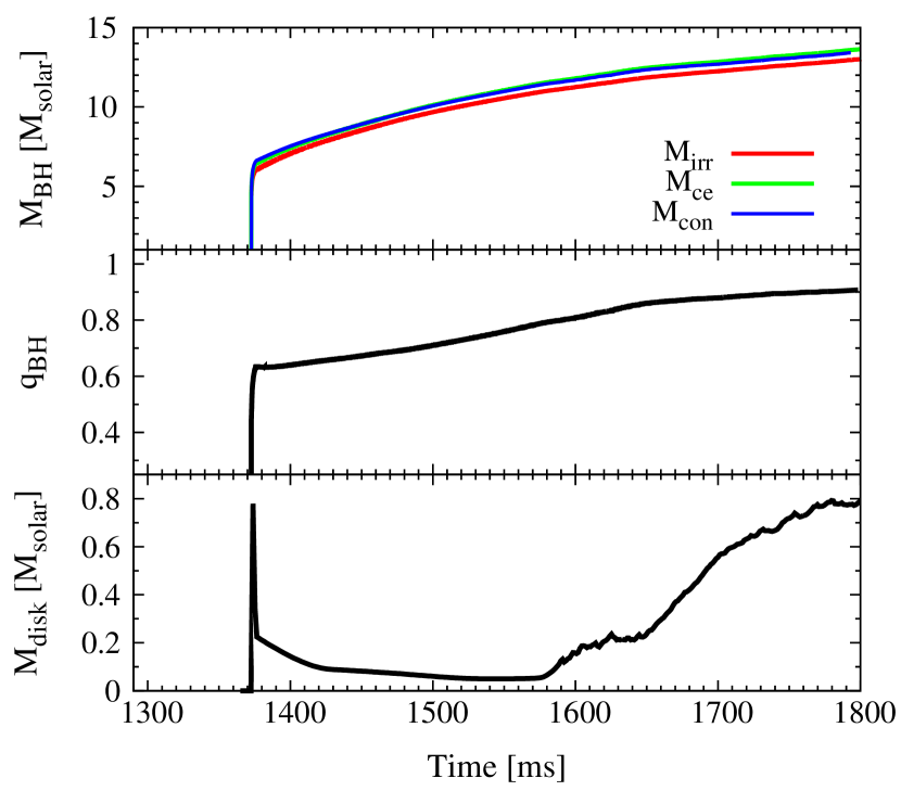
Figure 11.— Time evolution of mass (the top panel) and the non-dimensional spin parameter (the lower panel) of the black hole and disk mass (the bottom panel) for the moderately rotating model.

Figure 12.— Mass accretion rate into the black hole $dM_{\rm BH}/dt\equiv\dot{M}_{\rm BH}$ (the upper panel) and an efficiency of neutrino emission $L_{\nu}/\dot{M}_{\rm BH}c^{2}$ (the lower panel) as functions of time after the black hole (BH) formation for the moderately rotating model.

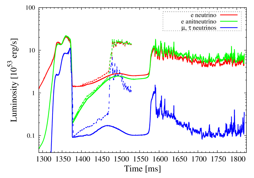
Figure 13.— Time evolution of neutrino luminosities for the moderately rotating model for the lower (solid curves) and finer (dashed curves) resolutions. A black hole is formed at $t\approx 1373$ ms.

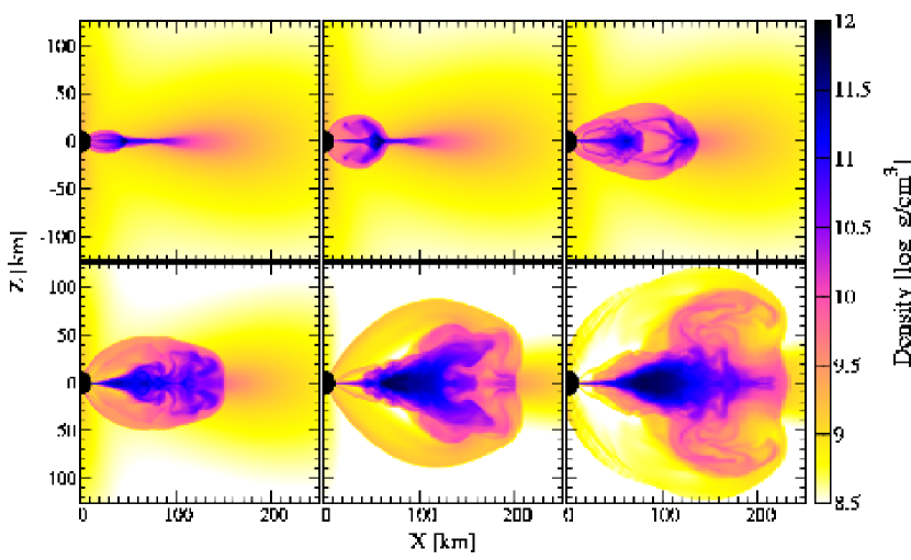
Figure 14.— Contours of rest mass density at $t\approx 1578$ (top left), 1584 (top middle), 1591 (top right), 1644 (bottom left), 1706 (bottom middle), and 1800 ms (bottom right) for the moderately rotating model.

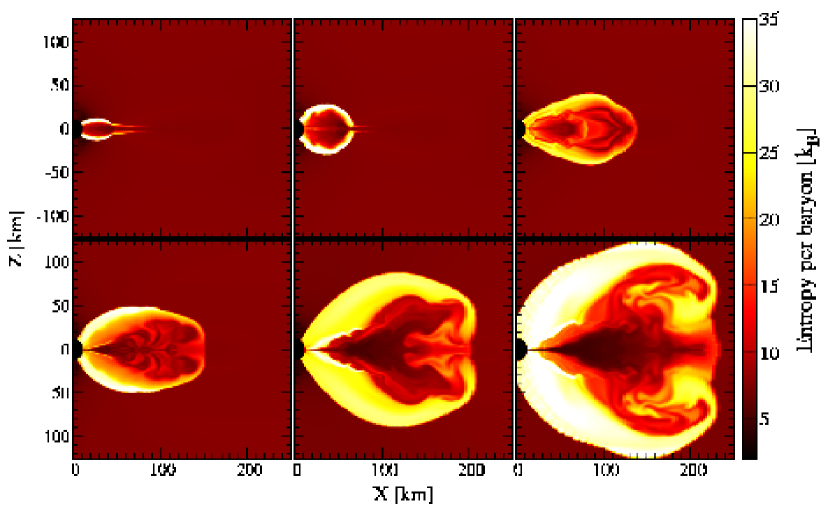
Figure 15.— Contours of entropy per baryon for the moderately rotating model. The selected time slices are the same as those in Figure 14.

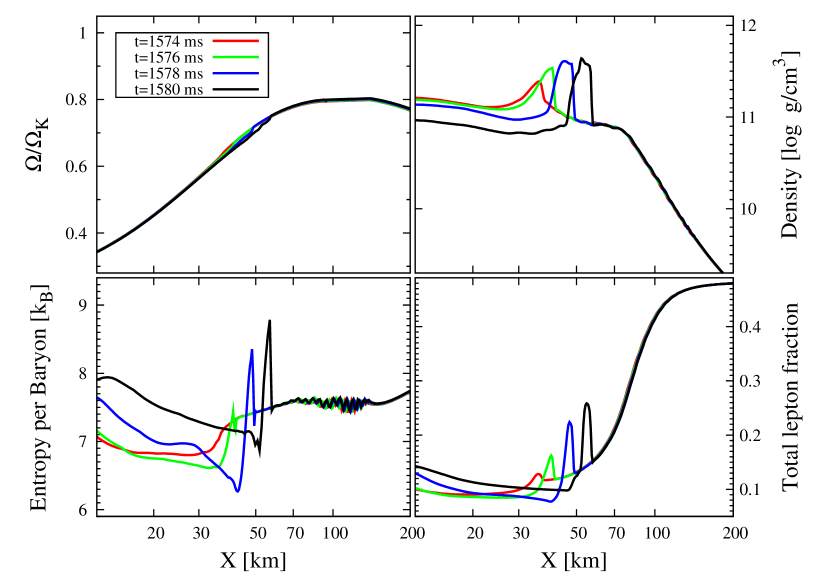
Figure 16.— Profiles of $\Omega/\Omega_{\rm K}$, density, entropy per baryon, and total lepton fraction along the radial direction in the equator at $t\approx 1574$, 1576, 1578, and 1580 ms.

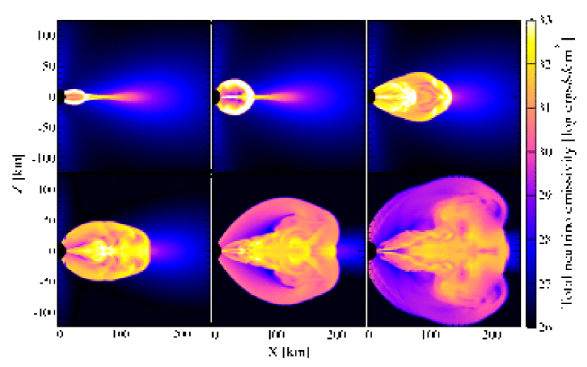
Figure 17.— Contours of the total neutrino emissivity for the moderately rotating model. The selected time slices are the same as those in Figure 14.

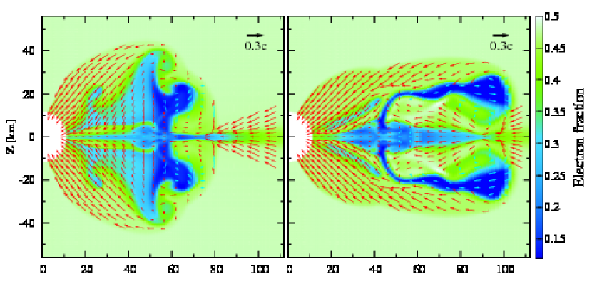
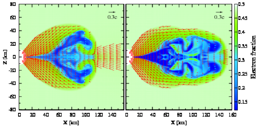
Figure 18.— Contours of electron fraction with velocity fields at $t\approx 1589$ (top left panel), 1590 (top right panel), 1596 (bottom left panel), and 1644 ms (bottom right panel).

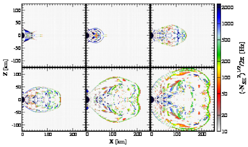
Figure 19.— Contours of the Solberg-Hoiland frequency for the moderately rotating model. The selected time slices are the same as those in Figure 14.

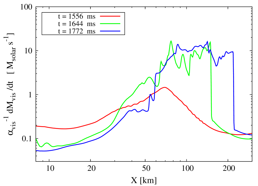
Figure 20.— Profiles of $\dot{M}_{\rm vis}$ along the radial direction in the equator in the geometrically-thin-disk phase (at $t\approx 1556$ ms) and the convective phase (at $t\approx 1644$ and $1574$ ms).

The basic features of rotational core collapse until the black hole formation are qualitatively the same as those of the spherical model: Gravitational collapse is triggered primarily by the photo-dissociation of heavy nuclei; the gas-pressure-dominated bounce occurs at a subnuclear density; a weak shock wave is formed at the bounce and is stalled quickly; a black hole is formed soon after the bounce in $\approx 30$–50 ms. After the black hole formation, on the other hand, the dynamics of infalling material is modified by the centrifugal force; an accretion disk is formed around the black hole as the material with sufficient specific angular momentum falls into the central region. We first describe the feature of the collapse for the moderately rotating model in Sections 3.2.1, 3.2.2 and 3.2.3. Then, we discuss dependence of the dynamics of the accretion disk formation and properties of the disk on the amount of rotation in Section 3.4. It is found that the process of the accretion disk formation and properties of the disk depend sensitively on the amount of rotation initially given.

3.2.1 Black hole and thin accretion disk formation

In this subsection, we describe features of dynamics of the first $\sim$ 200 ms after the black hole formation. We note that time duration of this phase depends on the grid resolution but the evolution process does not depend qualitatively on it. Figure 10 plots contours of density, electron fraction, entropy per baryon, and temperature at selected time slices around black hole formation epoch. As in the collapse for the spherical model, the weak bounce occurs at $t\approx 1339$ ms, and then, convectively unstable regions with negative gradients of electron fraction appear when the shock wave is stalled. However, because the core immediately collapses to a black hole, the convection is only weakly activated and plays a minor role (see the left and middle panels in Figure 10). Accompanied with the black hole formation, a geometrically thin, ’sub-Keplerian’ disk is formed around the black hole (see below for details). Note that the disk is geometrically thin not due to the neutrino cooling (because the disk is optically thick), but mainly due to the ram pressure of infalling material (see Eq. 57 and the discussion below).

Figure 11 plots the time evolution of mass and spin parameter of the black hole as well as disk mass ($M_{\rm disk}$). At $t\approx 1373$ ms, a black hole of $M_{\rm BH}\approx 6.5M_{\odot}$ with spin parameter of $q_{\rm BH}\approx 0.6$ is formed. The initial mass of the black hole is larger than that in the spherical collapse because the threshold mass for the black hole formation is larger due to effect of the rotation (the centrifugal force). Note that $M_{ce}$ seems to be a good indicator of mass of a black hole even in the presence of a massive accretion disk as suggested in Shibata (2007), because the time evolution of $M_{\rm con}$ and $M_{ce}$ approximately agrees with each other. The upper panel in Figure 12 plots the time evolution of mass accretion rate into the black hole ($\dot{M}_{\rm BH}$). The mass accretion rate soon (10 ms) after the black hole formation is high as $\dot{M}_{\rm BH}\approx 40M_{\odot}$ s^-1. The mass accretion rate decreases gradually with time, but even at $t\sim 1800$ ms, it is still as high as $\dot{M}_{\rm BH}\sim 5$–$10M_{\odot}$ s^-1 (see the upper panel in Figure 12).

Figure 13 plots the time evolution of neutrino luminosities for the moderately rotating model. As in the spherical model, electron neutrinos are dominantly emitted before the weak bounce, and electron neutrinos and electron anti-neutrinos are approximately identically emitted after the bounce. The luminosity curves of electron neutrinos ($\approx 1.6\times 10^{54}$ erg/s) and anti-neutrinos ($1.4\times 10^{54}$ erg/s) achieve the first peak soon after the weak bounce (at $t\approx 1330$ ms). By contrast with the spherical model, the second peak appears in the neutrino luminosity curves at $t\approx 1360$ ms. Because oblate (or torus-like) neutrino ’sphere’ is formed after the bounce due to the rotation, the optical depth of neutrinos is smaller in the $z$-direction (see the middle panels in Figure 10). As a result, neutrinos are more efficiently emitted in the $z$-direction and this effect constitutes the second peak. In this phase, more electron anti-neutrinos are emitted than electron neutrinos ($Q^{\rm ec}_{\nu_{e}}\lesssim Q^{\rm pc}_{\bar{\nu}_{e}}$) because the electrons inside the torus is only weakly degenerate $\eta_{e}\sim 1$ due to high temperature and the fraction of neutrons is larger than that of protons as $X_{p}/X_{n}\sim 0.2$, enhancing the reaction of $n+e^{+}\rightarrow p+\bar{\nu}_{e}$.

Soon after the black hole is formed, most of the material inside the oblate structure is quickly swallowed by the black hole because they do not have enough angular momentum to retain in the orbit around the formed black hole. However, a small amount of the material with sufficient angular momentum forms a geometrically thin accretion disk around the black hole (see the right panels in Figure 10). Mass of the geometrically thin disk just after the black hole formation is $M_{\rm disk}\approx 0.2M_{\odot}$ and subsequently decreases to be $\approx 0.1M_{\odot}$ (see the bottom panel in Figure 11) because material with high density located near the rotational axis, which does not have sufficient angular momentum and does not constitute the disk, is swallowed by the black hole. Then the thin-disk mass relaxes to a quasi-stationary value of $\sim 0.1M_{\odot}$ and the net mass infall rate onto the thin disk vanishes approximately ($\dot{M}_{\rm disk}\sim 0$). (For sudden increase of $M_{\rm disk}$ at $t\approx 1580$ ms, see Section 3.2.2.)

The rest mass density and temperature of the thin disk are initially $\sim 10^{11}$ g/cm³ and $\sim 8$ MeV (see Figure 10), and accordingly, the thin disk is optically thick to neutrinos with the maximum optical depth of $\tau_{\nu}\sim 4$ (which increases as the material with high angular momentum falls onto the thin disk). At the same time, shocks are formed in the inner part of the thin disk, converting kinetic energy of infalling materials into thermal energy (see Lee & Ramirez-Ruiz (2006) for discussion of a similar phenomenon).

The shock is successively formed due to infall of the material with angular momentum not large enough to retain the orbit around the black hole. After hitting the surface in the inner region of the disk, such material falls into the black hole quickly because of its insufficient specific angular momentum, and contributes to a rapid growth of the black hole. A part of the thermal energy generated at the shock is advected together into the black hole (see discussion below).

The thermal energy is also carried away by neutrinos because the cooling timescale of neutrino emission, $t_{\rm cool}$, is short due to the low density and small pressure scale height of the disk, $H$ (although the optical depth is greater than unity), as

$$t_{\rm cool}\sim\frac{H\tau_{\nu}}{c}\approx 0.12\,\left(\frac{H}{10\,{\rm km}}\right)\left(\frac{\tau_{\nu}}{4}\right)\,{\rm ms}.$$ (55)

This is much shorter than the advection time scale approximately given by

$$t_{\rm adv}\sim\frac{R_{\rm disk}}{v_{\rm adv}}\approx 1.7\,\left(\frac{R_{\rm disk}}{50{\rm km}}\right)\left(\frac{v_{\rm adv}}{0.1c}\right)^{-1}\,{\rm ms},$$ (56)

where $R_{\rm disk}(\approx r_{\rm ISCO}\gg H)$ and $v_{\rm adv}$ are characteristic radius of the disk and characteristic advection velocity.

The pressure scale height may be approximately determined by the following force balance relation (Sekiguchi & Shibata, 2007):

$${P_{\rm disk}-P_{\rm ram}\over H}\sim\frac{GM_{\rm BH}\rho_{\rm disk}H}{R_{\rm disk}^{\ 3}},$$ (57)

where $\rho_{\rm disk}$ and $P_{\rm disk}$ are characteristic density and pressure of the disk, and $P_{\rm ram}$ is the ram pressure of the infalling material, respectively. Equation (57) gives

$$\frac{H}{R_{\rm disk}}\sim\left(\frac{P_{\rm disk}-P_{\rm ram}}{10^{30}\ {\rm dyn/cm}^{2}}\right)^{1/2}\,\left(\frac{\rho_{\rm disk}}{10^{10}\ {\rm g/cm}^{3}}\right)^{1/2}.$$ (58)

Because the density and temperature retain to be low due to rapid advection and copious neutrino emission, $P_{\rm disk}\sim 10^{30}$ dyn/cm² is as small as the ram pressure, approximately written as

$$P_{\rm ram}\sim\rho_{\rm f}v_{\rm f}^{2}\sim 10^{30}\,\left(\frac{\rho_{\rm f}}{10^{10}\,{\rm g/cm}^{3}}\right)\ {\rm dyn/cm}^{2},$$ (59)

where $\rho_{\rm f}$ and $v_{\rm f}\sim(2GM_{\rm BH}/R_{\rm disk})^{1/2}\sim 0.4$–0.5$c$ are the density and velocity of the infalling material, respectively. Since $|P_{\rm disk}-P_{\rm ram}|\ll P_{\rm disk}$, the pressure scale height is very small as $H/R_{\rm disk}\ll 1$ in the early stage of the thin disk.

The lower panel in Figure 12 plots an efficiency of neutrino emission defined by $L_{\nu,{\rm tot}}/(\dot{M}_{\rm BH}c^{2})$, where $L_{\nu,{\rm tot}}$ is the total neutrino luminosity. The efficiency is low as $\sim 0.01$ in the thin accretion disk phase (until $\approx 200$ ms after the black hole formation). On the other hand, order of magnitude of the thermal energy generated at the shock in the inner region of the thin disk is estimated to give

$$\frac{GM_{\rm BH}\dot{M}}{r} \sim 0.1\dot{M}_{\rm BH}c^{2}$$ (60)

$$\sim 5\times 10^{54}\left(\frac{\dot{M}_{\rm BH}}{30M_{\odot}~{}{\rm s}^{-1}}\right)\,{\rm erg/s},$$

where $r\sim 0.1GM_{\rm BH}/c^{2}$ is the distance from the black hole. Here, it is assumed that most of the material falling onto the system experiences the shock heating (i.e., the total mass accretion rate $\dot{M}$ is used) and an approximation of $\dot{M}=\dot{M}_{\rm BH}+\dot{M}_{\rm disk}\approx\dot{M}_{\rm BH}$ is used.

Thus, the neutrino luminosity is by one order of magnitude smaller than that the energy generated at the shock. This indicates that the amount of material which experiences the shock heating is much smaller than that swallowed into the black hole because of small geometrical cross section with the disk. As the material with high specific angular momentum falls onto the disk and the size of the disk increases, neutrino luminosities and the shock heating efficiency increase (see Figure 13 and the lower panel in Figure 12). (For decrease of neutrino luminosities at $t\approx 1470$ ms, see Section 3.2.2.)

Because the total mass of the material surrounding the black hole is much larger than that in the spherical model, the neutrino luminosity remains high $>10^{53}$ erg/s even after the black hole formation (see Figure 13). For $\sim 200$ ms after the thin disk formation, the luminosity slightly increases but is kept to be $\sim 2\times 10^{53}$ erg/s. Because the duration of the neutrino emission from the thin disk is much longer than that before the black hole formation, neutrinos are likely to be primarily emitted from the accretion disk (torus), not during the black hole formation, in the moderately rotating model.

3.2.2 Disk expansion and torus formation

Figures 14 and 15 plot contours of density and entropy per baryon at selected time slices $\sim 200$–400 ms after the black hole formation. It is found that the geometrically thin accretion disk formed in the early stage expands to form a geometrically thick accretion torus. Note that the disk is also ’sub-Keplerain’ in this stage (see the top-left panel in Figure 16). The feature of dynamics can be explained as follows.

As the material with higher specific angular momentum in the outer region falls onto the disk, the density and mass of the disk increases (see the bottom panel in Figure 11). This situation is different from that in the early evolution of the geometrically thin disk, in which the material with small specific angular momentum dominantly falls. As a result, neutrino optical depth increases and neutrino cooling timescale becomes longer (cf. Eq. (55)). This helps further storing thermal energy inside the disk and the pressure scale height increases (see the top-left panel in Figure 15).

As the thermal energy is stored, the disk height $H$ increases according to Eq. (57). The density and the temperature ($T_{\rm disk}$) inside the disk eventually increase to be $\gtrsim 10^{11}$ g/cm³ and $\gtrsim 10$ MeV (and hence, $P_{\rm disk}\gtrsim 10^{30}$ dyn/cm²). At the same time, the ram pressure decreases to be $\lesssim 0.1P_{\rm disk}$ ($\ll P_{\rm disk}$) because the density of the infalling material decreases to $\lesssim 10^{9}$ g/cm³. Consequently, $H$ increases to be $\sim R_{\rm disk}$ (see the top-middle panels in Figures 14 and 15). For $H\gtrsim R_{\rm disk}$, the approximate force balance relation (57) changes to

$$(P_{\rm disk}-P_{\rm ram})\sim\frac{GM_{\rm BH}\rho_{\rm disk}}{H}.$$ (61)

Because the binding due to the gravitational force by the black hole decreases as $H$ increases, the disk expands forming a shock wave once the condition $H\gtrsim R_{\rm disk}$ is satisfied (Sekiguchi & Shibata, 2007). Figure 16 shows that the shock is formed at $t\approx 1576$ ms.

The neutrino opacities decrease as the disk expands (density and temperature decrease), and accordingly, the cooling timescale becomes shorter. Then, the shock wave is stalled and the disk relaxes to a new geometrically thick state. The shock becomes a standing accretion shock and expands gradually because the material with higher specific angular momentum continuously falls onto the shock and also because the ram pressure of the infalling material continues to decrease (see the bottom panels in Figures 14 and 15).

Note that when the pressure scale height, and thus, the optical depth become sufficiently large, the neutrino-cooling timescale becomes longer than the advection timescale into black hole, and consequently, neutrinos are trapped in the accretion flow. This can be seen in the time evolution of neutrino luminosities plotted in Figure 13: At $t\approx 1490$ ms, neutrino luminosities start decreasing slightly. The trapping of neutrinos are also found in a steady high-density accretion disk model (Di Matteo et al., 2002; Chen & Beloborodov, 2007). Note also that similar decrease of neutrino luminosities has been found in the simulations of ordinary core collapse soon after the onset of neutrino trapping (e.g., Liebendörfer et al., 2001).

Figure 17 plots contours of the total neutrino emissivity at selected time slices $\sim 200$–400 ms after the black hole formation. Neutrino luminosities are significantly enhanced after the thick torus formation. The reason for this is mainly that the amount of material which experiences the shock heating increases. The disk is optically thick to neutrinos at first and becomes optically thin as the disk expands. Then, neutrinos trapped inside the torus are emitted. This feature is somewhat similar to the so-called ’neutrino burst’ associated with the early shock formation in the ordinary supernova explosion.

After the expansion, the total luminosity reaches $\approx 2\times 10^{54}$ erg/s because amount of material which experiences the shock heating significantly increases. Then the efficiency of neutrino emission is as high as $L_{\nu,{\rm tot}}/(\dot{M}_{\rm BH}c^{2})\sim 0.1$ (see the lower panel in Figure 12). These agree approximately with the generation rate of thermal energy by infalling material on the standing shock,

$$\frac{GM_{\rm BH}\dot{M}}{r} \sim 0.1\dot{M}c^{2}$$ (62)

$$\sim 2\times 10^{54}{\rm erg/s}\left(\frac{\dot{M}}{10M_{\odot}~{}{\rm/s}}\right),$$

where a characteristic value of $\dot{M}=\dot{M}_{\rm BH}+\dot{M}_{\rm disk}\sim 10M_{\odot}$ s^-1 is adopted (see the bottom panel in Figure 11 and the upper panel in Figure 12). The high efficiency indicates that neutrino optical depth is not very high for the neutrino-emission region and that advection of the thermal energy into the black hole is not very large in this phase because of the quick neutrino emission.

3.2.3 Convective activities

After the formation of the geometrically thick torus, convective motions are excited near the shocked region in the torus. The origin of the convection is explained as follows.

The shock heating is more efficient in an inner part of the torus because kinetic energy of infalling material is larger (see the top-left panel in Figure 15). On the other hand, the neutrino cooling is less efficient in the inner part of the torus because of its higher density and resulting larger optical depth. Then, the entropy per baryon becomes higher in the shocked inner region of the torus (see Figure 15), and consequently, regions of negative entropy gradient along the radial direction near the equatorial plane are developed. Also, because neutrinos are trapped and $\beta$-equilibrium is achieved in the inner part of the torus, the total lepton fraction increases inward. These tendencies are enhanced as the accretion of the material with higher angular momentum proceeds.

The condition for convective instabilities to occur is given by the so-called Solberg-Hoiland criterion (e.g., Tassoul, 1978),

$$N_{\rm SH}^{\ 2}=N_{\rm BV}^{\ 2}+\kappa^{2}<0,$$ (63)

where $N_{\rm BV}$ is the Brunt-Väisälä frequency given by (e.g., Lattimer & Mazurek, 1981)

$$N_{\rm BV}^{\ 2} = \frac{g_{\rm eff}}{\rho}\left(\frac{\partial\rho}{\partial P}\right)_{s,Y_{l}}$$ (64)

$$\times\left[\left(\frac{\partial P}{\partial s}\right)_{\rho,Y_{l}}\left(\frac{ds}{dr}\right)+\left(\frac{\partial P}{\partial Y_{l}}\right)_{\rho,s}\left(\frac{dY_{l}}{dr}\right)\right],$$

and $\kappa$ is the epicyclic frequency which may be written for nearly circular orbits as (e.g., Binney & Tremaine, 1987)

$$\kappa^{2}=\varpi\frac{d\Omega^{2}}{d\varpi}+4\Omega^{2}.$$ (65)

Figure 16 plots the profiles of angular velocity, total lepton fraction, and entropy per baryon along the radial direction in the equator after the convection sets in. It is clearly shown that negative entropy gradient is formed in several regions inside the torus, and drives convection (see Figures 14 and 15). Rotation does not play an important role in suppressing the convective activities because the angular velocity $\Omega$ is smaller than the Kepler angular velocity given by

$$\Omega_{\rm K}=\left[\sqrt{\frac{r^{3}}{GM_{\rm BH}}}+q_{\rm BH}\frac{GM_{\rm BH}}{c^{3}}\right]^{-1},$$ (66)

(see the top-left panel in Figure 16), and thus, Coriolis force is not large enough.

The convective flows cannot move freely because the material infalling from the outside of the torus prevents the free expansion of the convective components (see the top-middle panel in Figure 14). Figure 18 plots contours of electron fraction with velocity fields. Interacting with the thin accretion flows, a part of the convective flows is swerved to form finger-like structure (see the top-right panel in Figure 18). Then, the convective components form a swirl. Note that regions with velocity shear appear at the interface between the convective fingers and the accretion flows (see the right panel in Figure 18), and hence, the Kelvin-Helmholtz instability could be developed at the interface, generating turbulent motions (see the bottom-left panel in Figure 18).

In addition, oscillations of the standing shock wave are induced. Such shock oscillations are proposed in a different context to explain quasi-periodic oscillations of X-ray binaries (Molteni et al., 1996) and found in a recent Newtonian simulation of sub-Keplerian accretion flows around a black hole (Giri et al., 2010).

Associated with the convective motions, many shock waves are formed and accretion flows show very complicated features. Because of interplay of the neutrino-trapping, the Kelvin-Helmholtz instability, and the convective shock, the accretion flow remains convectively unstable. Figure 19 shows the Solberg-Hoiland frequency, $N_{\rm SH}$ defined in Eq. (63). The effective gravity appeared in Eq. (64) is approximately evaluated using the Newtonian gravity as $g_{\rm eff}=GM_{\rm BH}/r^{2}$. As this figure shows, several regions inside the standing shock remain convectively unstable.

As a natural consequence of the convective activities of the accretion flow, neutrino luminosities vary violently in time (see Figure 13). If GRBs are driven by the pair annihilation of neutrinos and anti-neutrinos, such time-variability may explain the observed time-variability of GRB light curves. Furthermore, electrons in the convective regions are only weakly degenerate due to the high entropy and temperature. Consequently, the emissivities of electron neutrinos and electron anti-neutrinos are approximately identical ($Q^{\rm ec}_{\nu_{e}}\sim Q^{\rm pc}_{\bar{\nu}_{e}}$). This is favorable for the pair annihilation of neutrinos to electron-positron pairs because its rate is proportional to $L_{\nu}L_{\bar{\nu}}$ (see Section 4.3). We finally note that the total energies emitted in neutrinos over the entire time of the simulations are $E_{\nu,{\rm tot}}\approx 3.8\times 10^{53}$, $3.9\times 10^{53}$, and $9.4\times 10^{52}$ erg for electron neutrinos, electron anti-neutrinos, and total of $\mu$ and $\tau$ neutrinos.

3.2.4 Effect of viscosity and formation of viscous accretion disk

Finally we remark possible effects of viscosity in the evolution of the accretion disk, which are not taken into account in our simulation. Assuming that the disk (or torus) can be described by the standard disk model with $\alpha$-viscosity (Shakura & Sunyaev, 1973), mass accretion rate of disk material into the black hole due to the viscous transport of angular momentum ($\dot{M}_{\rm vis}$) is written as

$$\dot{M}_{\rm vis}\sim 4\pi\alpha_{\rm vis}PH\Omega^{-1},$$ (67)

where $\alpha_{\rm vis}$ is the viscous parameter and the pressure scale height is approximately estimated by

$$H\approx\sqrt{\frac{P}{\rho}\frac{r^{\ 3}}{GM_{\rm BH}}}\,.$$ (68)

Figure 20 plots characteristic values of $\dot{M}_{\rm vis}$ along the radial direction in the equatorial plane in the geometrically-thin-disk phase (at $t\approx$ 1556 ms), early (at $t\approx$ 1644 ms) and late (at $t\approx$ 1772 ms) stages of the convective phase. During the evolution of the accretion disk, viscosity is not likely to play an active role as described in the following.

In the geometrically-thin-disk phase, the predicted viscous mass accretion rate is small as $\dot{M}_{\rm vis}\lesssim 0.1M_{\odot}$ s^-1 for a relatively large viscous parameter of $\alpha_{\rm vis}=0.1$. Then characteristic timescale for viscous mass accretion is $\sim 1$ s because the disk mass is $M_{\rm disk}\sim 0.1M_{\odot}$ (see Figure 11), which is much longer than the duration of the geometrically-thin-disk phase $\sim 200$ ms.. Thus, the viscosity will not play an important role in the geometrically-thin-disk phase.

In the convective phase, the viscous mass accretion rate becomes large as $\dot{M}_{\rm vis}\sim M_{\odot}$ s^-1 for $\alpha_{\rm vis}=0.1$. On the other hand, the mass infall rate onto the torus is $\dot{M}_{\rm disk}\sim 3$–$4M_{\odot}$ s^-1 (see Figure 11), which is larger than the viscous mass accretion rate. Thus, effect of viscosity is not likely to play a central role and the disk will accumulate mass even in the presence of the viscosity.

The disk will spread outward with accumulating mass until the viscous mass accretion rate exceeds the infall mass accretion rate onto the disk ($\dot{M}_{\rm disk}\sim 4\pi R_{\rm disk}^{2}\rho_{\rm f}v_{\rm f}$). When $\dot{M}_{\rm disk}$ becomes smaller and the torus becomes more massive due to accretion of material from outer regions, the viscosity will play an important role on evolution and dynamics of the torus. Over the past decade, many groups have studied properties of the viscous accretion disk around a black hole (Popham et al., 1999; Narayan et al., 2001; Di Matteo et al., 2002; Kohri & Mineshige, 2002; Kohri et al., 2005; Gu et al., 2006; Chen & Beloborodov, 2007; Kawanaka & Mineshige, 2007). Such studies have successfully explained the energetics of LGRBs.

It should be note that in the viscous accretion phase, the material with low angular momentum will also fall in the vicinity of the black hole and shock dissipation of the infall kinetic energy will also occur. Material with high angular momentum can dissipate their infall kinetic energy on the standing shock before they reach the centrifugal barrier. The amount of such materials depends on the initial density and rotational profile yet poorly known. There might be substantial amount of mass accretion and energy generation due to such processes.

3.3. Dependence on grid resolution and numerical accuracy

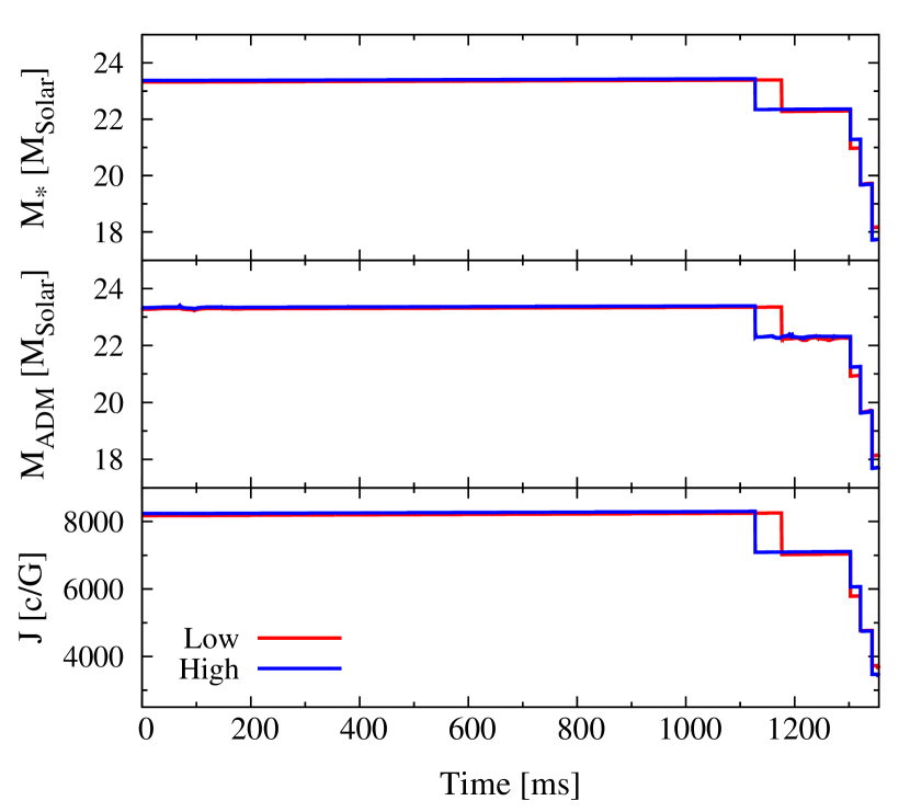
Figure 21.— Time evolution of the total baryon mass (the top panel), the total ADM mass (the middle panel), and the total angular momentum (the bottom panel) for the moderately rotating model. The red and blue curves correspond to the results in the lower resolution and in the higher resolution, respectively.

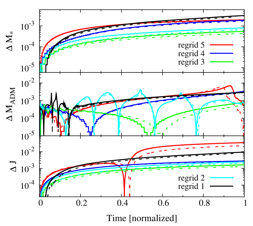
Figure 22.— Time evolution (normalized) in each regrid level of the total baryon mass (the top panel), the total ADM mass (the middle panel), and the total angular momentum (the bottom panel) for the moderately rotating model. The solid curves correspond to the results in the lower resolution and the dashed curves to those in the higher resolution.

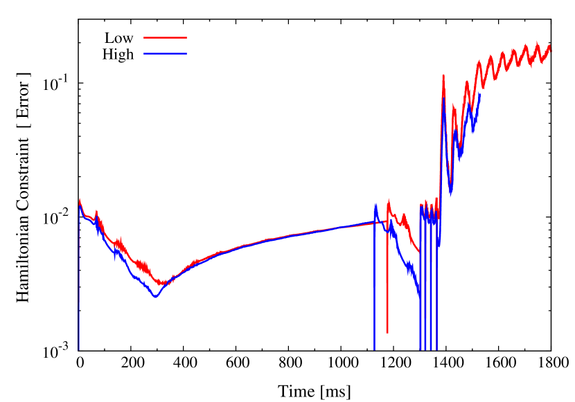
Figure 23.— Time evolution of the Hamiltonian constraint error for the moderately rotating model. The red and blue curves correspond to the results in the lower resolution and in the higher resolution, respectively.

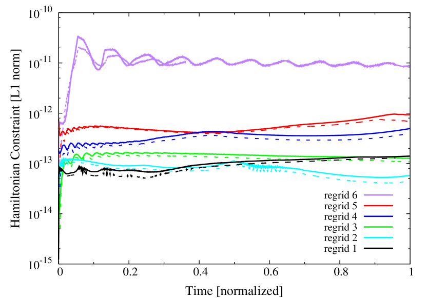
Figure 24.— Time evolution (normalized) in each regrid level of L1 norm of the Hamiltonian constraint for the moderately rotating model. The solid curves correspond to the results in the lower resolution and the dashed curves to those in the higher resolution.

Because the present simulation is long-term one, we here describe dependence of results on the grid resolution and numerical accuracy. In Figure 13, we compare the time evolution of neutrino luminosities derived both in the high (dashed curves) and low (solid curves) resolution runs. The neutrino luminosities in the two grid resolutions agree very well until the black hole formation, indicating that converged results are obtained for such phase. In the geometrically thin disk phase, on the other hand, the luminosities in the finer resolution are systematically higher than those in the lower resolution. This is because the vertical structure of the geometrically thin disk and shock-heated region are more accurately resolved in the finer resolution, and hence, the maximum temperature is higher in the finer resolution. Also, the geometrically thin disk more quickly expands to be the geometrically thick disk. This is because the thermal energy is more efficiently stored in the disk because neutrino opacities are larger due to the higher density and temperature. These results indicates the importance of resolving the vertical structure of the geometrically thin disk for the quantitative study. If the grid resolution is not sufficient, a geometrically thin disk may remain thin instead of expanding to be thick torus.

Note that the effects of grid resolution works in a positive manner in our results, that is, the transition of a thin disk to a thick disk is more likely to occur. We therefore safely conclude that qualitative feature of our results does not depend on the grid resolution.

To check the accuracy of our results, conservations of the baryon mass ($M_{*}$), the ADM mass ($M_{\rm ADM}$) (e.g, York, 1979), and the total angular momentum ($J$), as well as violations of the Hamiltonian constraint are monitored during the simulation. Figure 21 displays the time evolution of these quantities. The several discontinuous changes correspond to the regridding procedures where outer low density region which does not affect the evolution of the central region is discarded. In each regridding level, $M_{*}$, $M_{\rm ADM}$, and $J$ conserve well. To see this more quantitatively, we display the time evolution of error in each level of the regridding until the black hole formation in Figure 21. The error is given by

$$\Delta Q_{{\rm regrid\,}i}(t)=\left|\frac{Q_{{\rm regrid\,}i}(t)-Q_{{\rm regrid\,}i}(0)}{Q_{{\rm regrid\,}i}(0)}\right|,$$ (69)

where $Q_{{\rm regrid\,}i}$ denotes the conserved quantities $M_{*}$, $M_{\rm ADM}$, and $J$ in the $i$-th regrid level. For the purpose of facilitating visualization, the time is normalized by the duration of each regridding level.

The error of conservation of total baryon mass grows monotonically in time, while it is small as $O(10^{-3})$. A part of the error is caused by the outer boundary conditions for fluid quantities where a simple copy is imposed. The error of the ADM mass shows an oscillating behavior caused by the regridding procedure, and also is small as $\lesssim 1$%. The error in total angular momentum is also small as a few percent, indicating good accuracy of conservation. Note that after the black hole formation, we start to adopt the excision procedure in solving hydrodynamic equations, and consequently, these quantities do not conserve.

Figure 23 plots the time evolution of the Hamiltonian constraint error defined by Shibata (2003a)

$${\rm ERROR}={1\over M_{*}}\int\rho_{*}|V|d^{3}x,$$ (70)

$$V={\displaystyle\tilde{\Delta}\psi-{\psi\over 8}\tilde{R}+2\pi E\psi^{5}+{\psi^{5}\over 8}\tilde{A}_{ij}\tilde{A}^{ij}-{\psi^{5}\over 12}K^{2}\over\displaystyle|\tilde{\Delta}\psi|+\Big{|}{\psi\over 8}\tilde{R}\Big{|}+2\pi\rho_{h}\psi^{5}+{\psi^{5}\over 8}\tilde{A}_{ij}\tilde{A}^{ij}+{\psi^{5}\over 12}K^{2}},$$ (71)

where where $\psi\equiv e^{\phi}$, and $\tilde{\Delta}$ denotes the Laplacian with respect to $\tilde{\gamma}_{ij}$. Namely, we use $\rho_{*}$ as a weight factor for the average. This weight factor is introduced to monitor whether the main bodies of the system (inner cores and dense matter regions), in which we are interested, are accurately computed or not.

The several distinct spikes correspond to the regridding procedures where the Hamiltonian constraint equation is solved numerically. Until the black hole is formed, the constraint violation is very small as $\lesssim 10^{-2}$ and no signal of the increase is seen. After the black hole formation, degree of the violation becomes worse because of the excision procedure. However, the violation is still small as $\sim 10^{-1}$, indicating the good accuracy of the simulation. Note that the integration in Eq. (70) includes the inside the black hole. Figure 24 plots the time evolution (normalized) of the L1 norm of the Hamiltonian constraint in each regrid level. Again, the violation does not show the signal of rapid increase.

3.4. Dependence on rotation

In this section, we describe dependence of the formation process of the black hole and surrounding accretion disk, the convective activities inside the disk, and the emissivity of neutrinos, on the degree of initial rotation.

3.4.1 Slowly rotating model

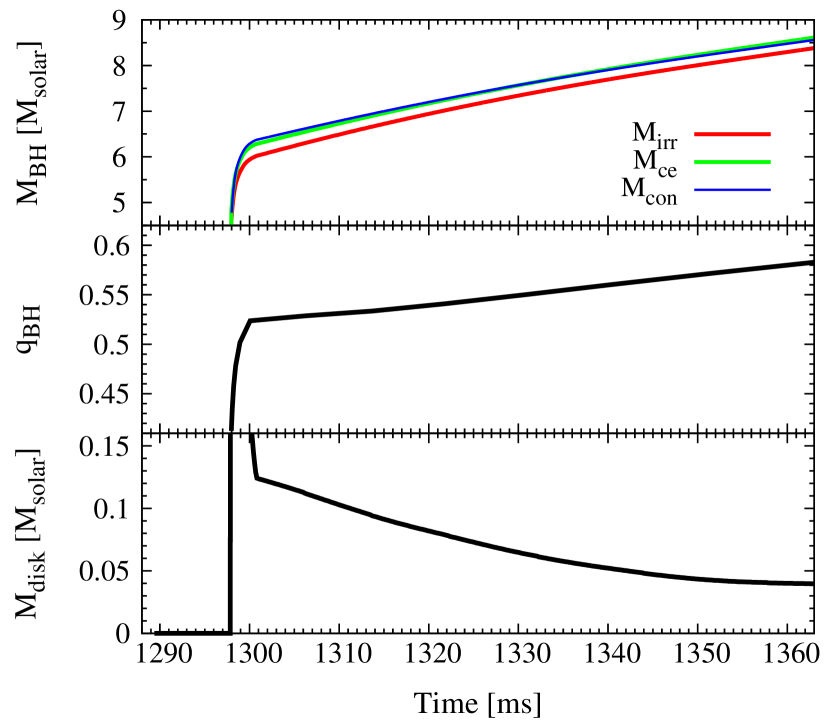
Figure 25.— Time evolution of mass (the top panel) and the non-dimensional spin parameter (the middle panel) of the black hole and disk mass (the bottom panel) for the slowly rotating model.

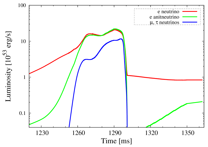
Figure 26.— Time evolution of neutrino luminosities for the slowly rotating model.

Figure 27.— Mass accretion rate into the black hole $dM_{\rm BH}/dt\equiv\dot{M}_{\rm BH}$ (the upper panel) and efficiency of neutrino emission $L_{\nu}/\dot{M}_{\rm BH}c^{2}$ (the lower panel) as functions of time after the black hole (BH) formation for the slowly rotating model.

In the slowly rotating model, a black hole with $M_{\rm BH}\approx 6.3M_{\odot}$ and $q_{\rm BH}\approx 0.53$ is formed at $t\approx 1298$ ms. The mass and spin parameter are only slightly smaller than those in the moderately rotating model. Figure 25 plots the time evolution of mass and spin parameter of the black hole as well as disk mass. The mass accretion rate into the black hole soon (10 ms) after the black hole formation is $\dot{M}_{\rm BH}\approx 45M_{\odot}$ s^-1 (see the upper panel in Figure 27), which is slightly larger than that in the moderately rotating model. The spin parameter remains modest but gradually increases as in the moderately rotating model.

As in the collapse of the moderately rotating model, a geometrically thin (but optically thick) accretion disk is formed soon after the black hole formation. In this case, a fraction of the material that forms the disk is smaller than that for the moderately rotating model due to lower specific angular momentum of fluid elements in the slowly rotating model, and hence, the disk mass is smaller as $M_{\rm disk}\sim 0.05M_{\odot}$ than that in the moderately rotating model and $\dot{M}_{\rm disk}<0$ (see the bottom panel in Figure 25). However, a part of the material that falls onto the disk still produces shock waves in the inner part of the disk. Thermal energy generated at the shock is not efficiently stored in the disk in the early stage because most of the shocked material is advected into the black hole and neutrinos carry away thermal energy. Then, the disk remains geometrically thin for a long time (at least $\gtrsim 100$ ms) after the formation of the black hole.

Figure 26 plots the time evolution of neutrino luminosities. Before the black hole formation, the luminosity curves are similar to those in the moderately rotating model. It is found that the geometrically thin accretion disk emits $\approx 10^{53}$ erg/s by neutrinos. This magnitude is by factor of $\sim 2$ smaller than that for the moderately rotating model. The efficiency of neutrino emission is $L_{\nu,{\rm tot}}/(\dot{M}_{\rm BH}c^{2})\approx 0.002$–0.003, which is by factor of $\sim 3$ smaller than that for the moderately rotating model (see the lower panel in Figure 27), indicating that less amount of material experiences the shock heating, and that more thermal energy is advected into the black hole before released by neutrinos due to slower rotation and resulting shorter advection timescale.

We do not find any enhancement of neutrino luminosity after the black hole formation in our simulation time. However, after the free-fall timescale of $\sim$seconds, the material with higher specific angular momentum may eventually form a dense disk. Then, thermal energy may be stored inside the disk, and the disk may expand to be a geometrically thick torus when the ram pressure of the infalling material becomes sufficiently small. Furthermore, provided that the total mass accretion rate is sufficiently high as $\dot{M}\gtrsim M_{\odot}$ s^-1, neutrinos will be trapped in the inner region of the disk, and convective activities may set in as in the moderately rotation model (see discussion in Section 4.1). If so, it is expected that neutrino luminosities are enhanced and show rapid time-variability as in the moderately rotating model.

3.4.2 Rapidly rotating model

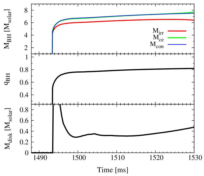
Figure 28.— Time evolution of mass (the top panel) and the non-dimensional spin parameter (the lower panel) of the black hole and disk mass (the bottom panel) for the rapidly rotating model.

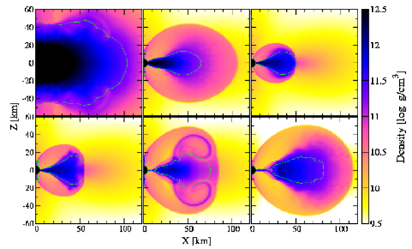
Figure 29.— Contours of rest mass density at $t\approx 1495$ (top left), 1497 (top middle), 1499 (top right), 1500 (bottom left), 1502 (bottom middle), and 1535 ms (bottom right) for the rapidly rotating model. The green curves indicate the region where $\tau_{\nu}=5$ for electron neutrinos.

Figure 30.— Mass accretion rate into the black hole $dM_{\rm BH}/dt\equiv\dot{M}_{\rm BH}$ (the upper panel) and efficiency of neutrino emission $L_{\nu}/\dot{M}_{\rm BH}c^{2}$ (the lower panel) as functions of time after the black hole (BH) formation for the rapidly rotating model.

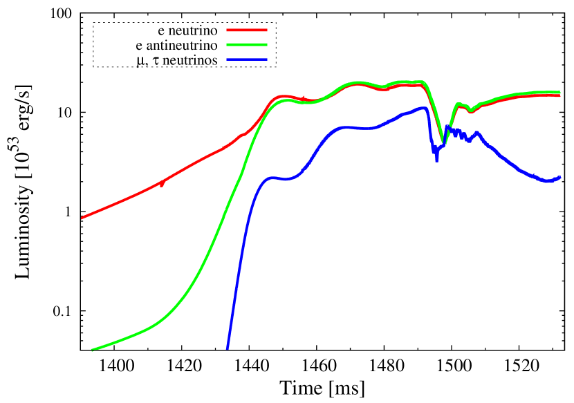
Figure 31.— Time evolution of neutrino luminosities for the rapidly rotating model. Note that the black hole is formed at $t\approx 1494$ ms.

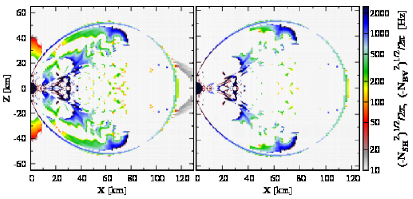
Figure 32.— Contours of the Brunt-Väisälä frequency (left panel) and the Solberg-Hoiland frequency defined by Eq. (63) (right panel) at $t\approx 1534$ ms for the rapidly rotating model.

In the rapidly rotating model, a black hole is first formed at $t\approx 1494$ ms with mass of $\approx 6.8M_{\odot}$ and the non-dimensional spin parameter of $\approx 0.8$. Figure 28 plots the time evolution of mass and spin parameter of the black hole together with disk mass. The spin parameter is much larger than that in the moderately rotating model as expected form Figure 4.

In the rapidly rotating model, the disk formation process is qualitatively different from that in the moderately rotating model. Figure 29 plots contours of rest mass density at selected time slices. The contour curve of $\tau_{\nu_{e}}=5$ is shown together as an approximate boundary of occurrence of the neutrino trapping. Inside this curve, neutrinos are trapped because $t_{\rm adv}(\sim R_{\rm disk}/v_{\rm adv}\sim R_{\rm disk}/0.1c)\sim t_{\rm cool}(\sim H\tau_{\nu}/c)$ for $R_{\rm disk}\sim 2H$.

In the moderately rotating model, a geometrically thin accretion disk is first formed, and then, it expands to be a geometrically thick torus. In the rapidly rotating model, by contrast, a geometrically thick torus is formed immediately after the black hole formation because the pressure gradient and the angular momentum of the fluid near the equator are large enough that it retains an orbit outside the ISCO. The disk at this phase is still ’sub-Keplerian’ with $\Omega/\Omega_{K}\approx 0.8$ at its maximum and the pressure gradient plays a role in the immediate torus formation. Reflecting the torus formation, $M_{\rm disk}$ is much larger as $\approx 0.4M_{\odot}$ than that in the slowly and moderately rotating models (see the bottom panel in Figure 28). Shock waves formed at the weak bounce are not swallowed into the black hole and a torus-shaped standing accretion shock remains around the black hole.

Associated with the torus formation, the mass accretion rate into the black hole just after the black hole formation shows non-monotonic behavior by contrast with the slowly and rapidly rotating models (see the upper panel in Figure 30). The mass accretion rate quickly drops to be $\dot{M}_{\rm BH}\approx 20M_{\odot}$ s^-1 at $t\approx 6$ ms after the black hole formation because of the centrifugal and pressure-supported hangup of the torus. The subsequent oscillating behavior is due to mass accretion associated with the oscillation of the torus. Then the mass accretion rate decreases quickly with time because the centrifugal force of the infalling material prevents the rapid accretion into the black hole. Note that the pressure gradient plays a role also in this phase. The mass accretion is expected to cease when $M_{\rm BH}\approx 12M_{\odot}$.

Figure 31 plots the neutrino luminosities as a function of time. Until the onset of the weak bounce (until the first local peak), the luminosity curves are similar to those in other models. After the weak bounce occurs, the material near the rotation axis starts collapsing, and as a result, the temperature increases due to compression and the optical depth near the rotation axis relatively decreases. Then, second local peak (at $t\approx 1475$ ms) associated with a substantial emission from the vicinity of rotation axis appears. This is the same feature as found in the slowly and moderately rotating models. In the rapidly rotating model, in addition, third local peak appears just before black hole formation at $t\approx 1494$ ms. This is due to the fact that a dense torus, which subsequently falls into the black hole, is formed (see the first panel in Figure 29) and emits a large amount of neutrinos just before swallowed by the black hole.

After the black hole formation, the luminosities decrease slightly. However, a dense torus surrounding the black hole is formed in a short time scale. Then, the luminosity increases again, and becomes as large as the second and third peaks with the total luminosity $\sim 3\times 10^{54}$ erg/s. Approximate generation rate of thermal energy at the shock on the surface of the torus due to infalling material is

$$\frac{GM_{\rm BH}\dot{M}}{r} \sim 0.1\dot{M}c^{2}$$ (72)

$$\sim 4\times 10^{54}\left(\frac{\dot{M}}{20M_{\odot}~{}{s^{-1}}}\right)\,{\rm erg/s}.$$

Thus, the neutrinos are emitted by converting infall kinetic energy of the material to the thermal energy.

Convective motions are also observed in the rapidly model as in the moderately rotating model. A large-scale circulation is formed associated with the formation of the thick, (mainly) centrifugally supported torus (see the bottom-middle panel in Figure 29). However, successive large-scale circulations, appeared in the moderately rotating model, do not occur in the rapidly rotating model, although small-scale convective activities are driven (see the bottom-right panel in Figure 29). This is due to the stabilizing effect of the epicyclic frequency (see Eq. (63)). Figure 32 plots the Brunt-Väisälä frequency (see Eq. (64)) and the Solberg-Hoiland frequency defined by Eq. (63). As shown in this figure, there exist regions with negative gradients of entropy per baryon and lepton fraction ($N^{\ 2}_{\rm BV}<0$) inside the thick torus (see the left panel in Figure 32). However, most of the low-frequency modes are suppressed by the stabilizing epicyclic mode and only the higher-frequency modes are present. Consequently, large-scale circulation modes are suppressed and only small-scale convective modes appear.

Due to the absence of large-scale convective modes, effects of the convection on neutrino luminosities are likely to be minor. Indeed, no violent time-variability is observed after the thick torus formation. The small bumps in luminosities at $t\approx 1500$–1510 ms are associated with the large-scale circulation (see the bottom-middle panel in Figure 29).

The total mass of the torus is $\sim 7$% of the black hole mass and gradually increases (see Figure 28). The self-gravity of the torus may play a role in a later phase; the torus may be unstable against non-axisymmetric perturbation and this may affect evolution of the torus because angular momentum transport and redistribution inside the torus are enhanced. To strictly clarify the evolution of such massive torus, a three-dimensional numerical simulation may be needed. This is one of the issues left for the future.

Finally, we remark possible effects of viscosity in the rapidly rotating model. Assuming that the torus can be described by the standard disk model, the mass accretion rate associated with a hypothetical viscous stress is estimated as $\dot{M}_{\rm vis}\sim 3$–$5M_{\odot}$ s^-1 for $\alpha_{\rm vis}=0.1$ (cf. Eq. (67)). Because the mass infalling rate onto the torus is $\dot{M}_{\rm disk}\approx 8M_{\odot}$ s^-1 at the late phase (see the bottom panel in Figure 28), the viscosity is not expected to play a crucial role for the evolution of the torus at an early phase simulated in this paper.

However, in a later phase, when the mass infalling rate onto the torus becomes smaller, the viscosity is expected to play an important role. Then, an ADAF-type (accretion dominated accretion flow) accretion flow may be the outcome in the presence of a large viscosity. A high-velocity outflow may be accompanied because the accretion rate is likely to be very high (e.g., Narayan et al., 2001). The high black hole spin may also play an important role for driving a high-velocity outflow because the heating rate is enhanced near the ISCO and the mass accretion is suppressed due to the small black hole radius.

4. Discussions

4.1. Effect of the black hole spin on disk property and neutrino emissivity

The black hole formed after the core collapse is in general not a Schwarzschild black hole but a rotating black hole ($q_{\rm BH}\gtrsim 0.5$ for our models). In addition, a high spin state with $q_{\rm BH}\gtrsim 0.8$ is easily achieved during the evolution of the black hole. Thus, it is necessary to take into account the effects associated with such a high black hole spin to build plausible models in the collapsar scenario.

The spin of a black hole is known to play a crucial role on the evolution of the accretion disk (Chen & Beloborodov, 2007). The inner edge of the disk (or torus) around a rapidly rotating black hole comes closer to the black hole than that around a Schwarzschild black hole, and consequently, the temperature and density of the disk reach higher values. These significantly enhance neutrino luminosities. In addition, due to the higher density and temperature, the disk becomes more opaque to neutrinos, and neutrinos are often trapped in the inner regions of the disk. This leads to formation of regions with negative entropy gradient, and convection is induced. As a result of convection, neutrino luminosity curves may become highly variable.

Here, it should be noted that the trapping of neutrinos and occurrence of convective motions are not likely to be special consequences of the high mass accretion rate ($\dot{M}\sim 10M_{\odot}$ s^-1) achieved in our models. According to results of a general relativistic study by Chen & Beloborodov (2007), the neutrino trapping occurs even with a moderate mass accretion rate of $\dot{M}\sim M_{\odot}$ s^-1 for accretion flows around a rapidly rotating Kerr black hole. For accretion flows around a Schwarzschild black hole, by contrast, the neutrino trapping does not occur even with a high mass accretion rate of $\dot{M}\sim 10M_{\odot}$ s^-1 (Chen & Beloborodov, 2007). This illustrates that the black hole spin plays a crucial role on the properties of accretion flows around a black hole. They also find that the neutrino trapping occurs in the vicinity of the black hole ($r\lesssim 20GM_{\rm BH}/c^{2}$), as in our case. This indicates the importance of resolving the regions in the vicinity of the black hole because the seed of convection is formed there. (We note that the enhancement of neutrino luminosities due to the convection was not found in previous pseudo-Newtonian studies because a rather wide region near the black hole was excised in these studies.)

4.2. Comparison with CDAFs

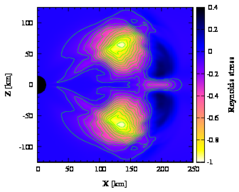
Figure 33.— The $r\varphi$-component of the Reynolds stress tensor ${{\hbox{\boldmath$t$}}}_{r\varphi}$ normalized so that the maximum amplitude of negative sign is unity.

Presence of convective accretion flow, named as convection-dominated accretion flow (CDAF), was first predicted by Narayan & Yi (1994) in their studies of a self-similar solution of advection-dominated accretion flows (ADAFs). Later, CDAFs were found in numerical studies of ADAFs around a black hole (Stone et al., 1999; Igumenshchev & Abramowicz, 2000). They found as a remarkable property of CDAF that the convection transports the angular momentum inward rather than outward.

To see whether this is the case in the present simulation, we calculate the $r\varphi$-component of the Reynolds stress tensor, ${{\hbox{\boldmath$t$}}}_{r\varphi}=\langle\delta v_{r}\delta v_{\varphi}\rangle$, where $\delta v_{i}=v_{i}-\langle v_{i}\rangle$ is the velocity fluctuation and $\langle\ \ \rangle$ denotes time-averaging (Igumenshchev & Abramowicz, 2000). Note that negative (positive) sign of ${{\hbox{\boldmath$t$}}}_{r\varphi}$ corresponds to the inward (outward) transfer of the angular momentum. Figure 33 plots contour of ${{\hbox{\boldmath$t$}}}_{r\varphi}$ in the $x$-$z$ plane. This figure clearly shows that there are regions with negative values of ${{\hbox{\boldmath$t$}}}_{r\varphi}$ near the outer surface of the torus. Convection in these regions transports the angular momentum inward, generating flows with higher angular momentum in an inner region. Such flows will then move outward forming circulations.

While the CDAF-like accretion flows are formed in the outer part of the torus, flows in the inner region are similar to those of neutrino-dominated accretion flows (NDAFs) (Popham et al., 1999). Furthermore, the torus is accompanied by the quasi-radial flows which consist of the material with low angular momentum and the outer geometrically thin accretion flows near the equatorial plane. Narayan et al. (2001) found that transition between CDAF and NDAF are determined by a characteristic radius $r_{\rm out}$: Flows injected from $r\gtrsim r_{\rm out}$ form CDAFs, and those injected from $r\lesssim r_{\rm out}$ form NDAFs. In terms of the specific angular momentum, transition between CDAF and NDAF may be determined by a characteristic specific angular momentum $j_{\rm out}$: The material with $j\gtrsim j_{\rm out}$ form CDAFs and those with $j\lesssim j_{\rm out}$ form NDAFs. As found in the present simulation, the accretion flows in the moderately rotating collapsar model will be characterized by the inner NDAF-like and outer CDAF-like parts.

4.3. Application to Gamma-ray bursts

We now turn to application of our results to LGRBs. We consider, as two possible ways of the energy deposition process, the neutrino pair annihilation and the Blandford-Znajek process (Blandford & Znajek, 1977). Because both of which processes are not included in our numerical simulation, we give an order estimate of the energy deposition rates for the purpose of clarifying the potential of driving relativistic jets in our models.

The annihilation rate of neutrinos and anti-neutrinos into electron-positron pairs has been calculated as a mechanism to power GRBs by several groups (Ruffert et al., 1997; Popham et al., 1999; Asano & Fukuyama, 2000, 2001; Salmonson & Wilson, 2001; Setiawan et al., 2004, 2006; Birkl et al., 2007; Harikae et al., 2010a, b; Zalamea & Beloborodov, 2011). The energy from the neutrino pair annihilation should be deposited in a baryon-poor region in order to generate highly relativistic outflows. The funnel region near the rotational axis above the torus is a promising place for this purpose.

Here, we an order estimate of the total energy deposition rate by the neutrino pair annihilation ($\dot{E}_{\nu\bar{\nu}}$). The deposition rate is proportional to $\dot{M}^{9/4}M_{\rm BH}^{-3/2}$ (Beloborodov, 2008). In this estimation, the neutrino luminosity is assumed to be originated from a viscous heating. In our present calculation, the neutrino luminosity is determined by mass accretion rate of the infalling material which experiences the shock heating and increases thermal energy of the disk. However, the dependence of the pair-annihilation rate on the mass infall rate $\dot{M}$ is essentially the same for thick torus phase. Due to this strong dependence on the mass accretion rate, the energy deposition by the neutrino pair-annihilation will be important only for an early phase of the LGRB formation.

In the geometrically thin disk, the efficiency of the neutrino pair annihilation for a rapidly rotating black hole may be written, according to a recent general relativistic study by Zalamea & Beloborodov (2011), as

$$({\rm eff})_{\nu\bar{\nu}}\equiv\frac{\dot{E}_{\nu\bar{\nu}}}{L_{\nu,\,{\rm tot}}}\sim 0.01\left(\frac{\dot{M}}{M_{\odot}\,{\rm s}^{-1}}\right)^{5/4}\left(\frac{M_{\rm BH}}{10\,M_{\odot}}\right)^{-3/2},$$ (73)

where $L_{\nu,\,{\rm tot}}$ is the total neutrino luminosity. In the present simulation, the expected energy deposition rate by neutrino pair annihilation is quite high as $\dot{E}_{\nu\bar{\nu}}\sim 10^{53}$ erg/s for $M_{\rm BH}\sim 10M_{\odot}$, $\dot{M}\sim 10M_{\odot}$ s^-1, and $L_{\nu,\,{\rm tot}}\sim 10^{54}$ erg/s in an early phase of disk evolution for $\sim 1$ s.

The efficiency of the neutrino pair annihilation depends strongly on the geometry of the disk. In particular, (eff)${}_{\nu\bar{\nu}}$ is proportional to $V^{-1}_{\rm ann}$, where $V_{\rm ann}$ is characteristic volume above the disk (Mochkovitch et al., 1993; Liu et al., 2010; Zalamea & Beloborodov, 2011). Liu et al. (2010) calculated the vertical structure of geometrically-thick accretion flows in the pseudo-Newtonian gravity and estimated the energy deposition rate. They found that the efficiency could be enhanced by an order of magnitude. In this case, a very large energy deposition rate by neutrino pair annihilation of $\dot{E}_{\nu\bar{\nu}}\sim 10^{54}$ erg/s may be expected.

The outgoing Poynting power at the horizon in the Blandford-Znajek process is given by (Blandford & Znajek, 1977; Thorne et al., 1986)

$$\dot{E}_{\rm BZ}\approx\frac{c}{32}\,q_{\rm BH}^{2}\,(B_{H}^{\perp})^{2}\,R_{H}^{2}\,\frac{\Omega_{B}(\Omega_{H}-\Omega_{B})}{\Omega_{H}^{2}},$$ (74)

where $B_{H}^{\perp}$ is magnitude of magnetic fields normal to the horizon, $R_{H}\sim GM_{\rm BH}/c^{2}$ is the radius of the horizon, and $\Omega_{H}$ and $\Omega_{B}$ are the angular velocities of the horizon and the magnetic field lines.

McKinney (2005) suggested an approximate fitting formula for the estimation of the field strength based on results of general relativistic magnetohydrodynamical simulations. According to his formula, the outgoing Poynting power in the Blandford-Znajek process is given by

$$\dot{E}_{\rm BZ}\sim 10^{52}\,f_{\Omega_{H}}\,q_{\rm BH}^{2}\left(\frac{\dot{M}}{M_{\odot}\,{\rm s}^{-1}}\right)\,{\rm erg/s},$$ (75)

where $f_{\Omega_{H}}$ is a parameter which depends strongly on the angular velocity and the most optimistic condition $\Omega_{B}=\Omega_{H}/2$ is assumed. According to the result of McKinney (2005), $\gtrsim 10$% of the total outgoing power may be used to produce the LGRB jet. Thus, the outgoing jet power will be $\dot{E}_{\rm BZ,jet}\sim 10^{51}f_{\Omega_{H}}q^{2}_{\rm BH}(\dot{M}/(M_{\odot}\,{\rm s}^{-1}))$ erg/s for our models.

The Blandford-Znajek power will eventually become much larger than the deposition rate by the neutrino pair-annihilation because the power depends more weakly on the mass accretion rate. Even in a late phase with $\dot{M}\sim 0.1M_{\odot}$ s^-1, a jet power of $\dot{E}_{\rm BZ,jet}\sim 10^{51}$ erg/s may be achieved if the black hole is sufficiently rapidly rotating ($q_{\rm BH}\gtrsim 0.9$ for which $f_{\Omega_{H}}\gtrsim 10$), accumulating the angular momentum of infalling material. Note also that magnetic fields may be amplified in the torus due to the magneto-rotational instability and/or convection (Balbus & Hawley, 1991, 1998).

4.4. Gravitational waves from anisotropic neutrino emission

A cosmological population of core-collapse supernovae is one of the most important sources of gravitational wave backgrounds (Buonanno et al., 2005). Gravitational waves (GWs) associated with anisotropic neutrino emission are particularly important because they generate a burst of GWs accompanying with the memory effect, the so-called burst with memory (Braginskii & Thorne, 1987). GW memory due to anisotropic neutrino emission could contaminate, at low frequencies around 0.1Hz, the inflationary GW (Buonanno et al., 2005; Hiramatsu et al., 2005; Suwa et al., 2007a), which is one of the targets of future space GW detectors such as DECIGO (Seto et al., 2001) and BBO (Ungarelli et al., 2005). Here, we give an order estimate of the amplitude of GWs associated with anisotropic neutrino emission.

The amplitude of GWs due to anisotropic neutrino emission is given by (Mueller & Janka, 1997; Kotake et al., 2007; Suwa & Murase, 2009). Taking characteristic values of total neutrino luminosity of $\sim 10^{54}$ erg/s from our simulation results and assuming a duration of neutrino emission of $\Delta t_{\nu}\sim 1$ s (cf. the moderately rotating model), the amplitude may be estimated as

$$h_{\nu}\sim 2\times 10^{-24}\left(\frac{10\,{\rm Gpc}}{D}\right)\left(\frac{L_{\nu}}{10^{54}\,{\rm erg/s}}\right)\left(\frac{\Delta t_{\nu}}{1\,{\rm s}}\right),$$ (76)

where $D$ is the distance to the source. This value is as large as that calculated by Suwa et al. (2007a) for the collapse of $300M_{\odot}$ PopIII stellar core collapse. Note that the initial core mass in Suwa et al. (2007a) is about three times larger than ours. The peak neutrino luminosities achieved in their results are by a factor of $\sim 10$ larger than those in our results, while the duration in their results is by a factor of $\sim 10$ shorter than that in the moderately rotating model, because they failed to find convective activities in the accretion torus.

If long-term neutrino emission as found in the present simulations is universal for the Pop III stellar collapse, the GW memory due to anisotropic neutrino emission could significantly contaminate the inflationary GW.

5. Summary

In this paper, we performed axisymmetric simulations of very massive stellar core collapsing to a system composed of a rotating black hole and surrounding disk in full general relativity. We took into account a nuclear-theory-based finite-temperature EOS (Shen’s EOS), weak interaction processes such as electron capture and pair-neutrino processes, and neutrino cooling, which is handled by a general relativistic leakage scheme (Sekiguchi, 2010a, b).

Progenitor models of LGRBs suggested in the literatures (e.g., Fryer et al., 2007)) raise a possibility that they may have an entropy higher than that of ordinary supernova cores. In this work, we employed a core with a high entropy of $s/k_{B}=8$ as the initial condition. Because the distribution of angular momentum in very massive stars is highly uncertain, we employed four models (spherical, slowly rotating, moderately rotating, and rapidly rotating models) by superimposing a profile of rotational angular velocity in a parametric manner. The initial models adopted in this paper are not rapidly rotating in the sense that the rotation velocity imposed is much smaller than that required to retain the ISCO around a Schwarzschild black hole and that considered in previous studies (e.g., MacFadyen & Woosley (1999), see also Lopez-Camara et al. (2009) and references therein).

As in the collapse of ordinary supernova cores, gravitational collapse sets in due to photo-dissociation of heavy nuclei and electron capture. However, the collapse dynamics and properties of neutrino emission are different from those of ordinary supernova cores. The characteristics of the collapse of high-entropy cores are summarized as follows:

1. The gravitational contraction is decelerated by the thermal gas-pressure of free nucleons at a subnuclear density and the core experiences a weak bounce (the gas-pressure-dominated bounce). This is a result of the high entropy. We reconfirmed this previous discovery (Nakazato et al., 2007; Suwa et al., 2007b) and clarified the physical origin in detail: We clarified that the weak bounce is universal for the collapse of the core with $s/k_{B}\approx 5$–16.

2. Because the gas-pressure-dominated bounce is too weak to halt the infalling material, a black hole is formed soon after the bounce (within $\sim 30$ ms). The mass of the black hole at the moment of its formation ($\sim 5.8$–$7M_{\odot}$) is much larger than the maximum mass of a cold neutron star ($\approx 2.2M_{\odot}$for the Shen’s EOS). This is also due to the high entropy (high thermal pressure). Just before the black hole formation, the pair-neutrino production processes are enhanced because the temperature increases due to the adiabatic compression (due to neutrino trapping). As a result, approximately the same amount of electron neutrinos and anti-neutrinos are emitted. The mass accretion rate into the black hole just after the black hole formation and the total neutrino luminosity just before the black hole formation are $\sim 40M_{\odot}$ s^-1 and $\sim 4\times 10^{54}$ erg/s depending weakly on the degree of rotation. Thus the maximum efficiency for the neutrino emission is $L_{\nu}/(\dot{M}c^{2})\sim 6$%.

3. In the moderately rotating model, a geometrically thin accretion disk is first formed around the black hole and shocks are formed on its surface, generated by the infalling material. As the thermal energy is stored in the disk, it expands eventually to be a geometrically thick accretion torus. After the thick torus formation, convective activities, which are similar to those in CDAFs (Narayan et al., 2001), set in because a region with negative entropy gradient emerges in the inner part of the torus, due to occurrence of the neutrino trapping. The neutrino luminosities are $L_{\nu_{e}}+L_{\bar{\nu}_{e}}\sim 10^{54}$ erg/s, and show violent time-variability. Here we emphasize that the source of thermal-energy generation, which is eventually dissipated by neutrinos, is the shock heating of infalling materials. The high spin of a black hole is likely to play a crucial role on the evolution of the accretion disk, convective activities, and the enhancement of neutrino luminosities.

4. The evolution process of the accretion disk and neutrino emissivity depend strongly on the degree of initial rotation. In the slowly rotating model, the disk remains geometrically thin for a long time, and hence, the neutrino emissivity also remains relatively small ($L\sim 10^{53}$ erg/s) for more than 100 ms. In the rapidly rotating model, by contrast, a geometrically thick torus is immediately formed after the black hole formation, and luminosities of neutrinos emitted from the torus are as high as $10^{54}$ erg/s even at its formation. However, the convection is suppressed by the stabilizing epicyclic mode due to the rapid rotation and no violent time-variability is observed in the neutrino luminosities.

5. Irrespective of the degree of rotation, long-lived disk or torus surrounding the black hole is a primary emitter of neutrinos because of its high luminosity and long lifetime $\mathrel{\raise 1.29167pt\hbox{$>$}\mkern-14.0mu\lower 2.58334pt\hbox{$\sim$}}1$ s. This implies that anisotropic emission of neutrinos comes mainly from the accretion disk (torus) surrounding a black hole, not from the dense matter collapsing to a black hole. For a correct estimation of gravitational-wave background by anisotropic neutrino emission, it may be necessary to understand the physical condition of the accretion disk or torus (see below).

Finally, we comment on major limitations of the present study. First, we adopt initial conditions which are not based on latest theoretical models of stellar evolution. We are going to perform simulations adopting more realistic initial models soon. Second, the present simulations are performed on the assumption of axial symmetry. The accretion disk formed in the present simulations may become unstable against non-axisymmetric instabilities (e.g., Korobkin et al., 2011; Taylor et al., 2011; Kiuchi et al., 2011). Competition between non-axisymmetric instabilities and convective instabilities should be explored. Third, we do not take account of the neutrino heating. A simple approximated procedure of including effects of neutrino heating is adopted by O’Connor & Ott (2011) in which stellar core collapse to a black hole is studied by a spherically symmetric fully general relativistic simulation. We also plan to study effects of neutrino heating using a recently developed formulation (Shibata et al., 2011). Fourth, we do not consider effects of magnetic fields which will play a role during the collapse (e.g., Barkov & Komissarov, 2008; Komissarov & Barkov, 2009) and subsequent evolution of the disk (e.g., Penna et al., 2010; Barkov & Baushev, 2011) if progenitor cores have large magnetic fields. We plan to perform simulations taking account of magnetic fields using a general relativistic magnetohydrodynamic code we have developed (Shibata & Sekiguchi, 2005).

References

- Abel et al. (2002) Abel, T., Bryan, G. L., & Norman, M. L. 2002, Science, 295, 93
- Alcubierre & Brügmann (2001) Alcubierre, M., & Brügmann, B. 2001, Phys. Rev. D, 63, 104006
- Alcubierre et al. (2001) Alcubierre, M., Brügmann, B., Holz, D., Takahashi, R., Brandt, S., Seidel, E., Thornburg, J., & Ashtekar, A. 2001, Int. J. Mod. Phys. D, 10, 273
- Asano & Fukuyama (2000) Asano, K., & Fukuyama, T. 2000, ApJ, 531, 949
- Asano & Fukuyama (2001) Asano, K., & Fukuyama, T. 2001, ApJ, 546, 1019
- Balbus & Hawley (1991) Balbus, S. A., & Hawley, J. F. 1991, ApJ, 376, 214
- Balbus & Hawley (1998) Balbus, S. A., & Hawley, J. F. 1998, Rev. Mod. Phys., 70, 1
- Barkov & Baushev (2011) Barkov, M. V., & Bauchev, A. N. 2011, New. Astron., 16, 46
- Barkov & Komissarov (2008) Barkov, M. V., & Komissarov, S. S. 2008, MNRAS, 385, L28
- Baumgarte & Shapiro (1999) Baumgarte, T. W., & Shapiro, S. L. 1999, Phys. Rev. D, 59, 024007
- Beloborodov (2008) Beloborodov, A. M. 2008, in AIP Conf. Proc. 1054, Cool Discs, Hot Flows: The Varying Faces of Accreting Compact Objects, ed. M. Axelsson (Melville, NY: AIP), 51
- Binney & Tremaine (1987) Binney, J., & Tremaine, S. 1987, Galactic Dynamics (Princeton, NJ: Princeton Univ. Press)
- Birkl et al. (2007) Birkl, R., Aloy, M. A., Janka, H.-T., Müller, E. 2007, A&A, 463, 51
- Blandford & Znajek (1977) Blandford, R. D., & Znajek, R. L. 1977, MNRAS, 179, 433
- Bond et al. (1984) Bond, J. R., Arnett, W. D., & Carr, B. J. 1984, ApJ, 280, 825
- Braginskii & Thorne (1987) Braginskii, V. B., & Thorne, K. S. 1987, Nature, 327, 123
- Bromm et al. (2002) Bromm, V., Coppi, P. S., & Larson, R. B. 2002, ApJ, 564, 23
- Bromm & Loeb (2006) Bromm, V., & Loeb, A. 2006, ApJ, 642, 382
- Bruenn (1985) Bruenn, S. W. 1985, ApJS, 58, 771
- Brügmann et al. (2008) Brügmann, B., González, J. A., Hannam, M., Husa, S., Sperhake, U., & Tichy, W. 2008, Phys. Rev. D, 77, 024027
- Buonanno et al. (2005) Buonanno, A., Sigl, G., Raffelt, G. G., Janka, H.-T., Müller, E. 2005, Phys. Rev. D, 72, 084001
- Burrows et al. (2006) Burrows, A., Reddy, S., & Thompson, T. A. 2006, Nucl. Phys. A, 777, 356
- Campana et al. (2006) Campana, S., et al. 2006, Nature, 442, 1008
- Campana et al. (2008) Campana, S., et al. 2008, ApJ, 683, L9
- Campanelli et al. (2006) Campanelli, M., Lousto, C. O., Marronetti, P., & Zlochower, Y. 2006, Phys. Rev. Lett., 96, 111101
- Cantiello et al. (2007) Cantiello, M., Yoon, S.-C., Langer, N., & Livio, M. 2007, A&A, 465, L29
- Chen & Beloborodov (2007) Chen, W.-X., & Beloborodov, A. M. 2007, ApJ, 657, 383
- Christensen et al. (2004) Christensen, L., Hjorth, J., & Gorosabel, J. 2004, A&A, 425, 913
- Cobb et al. (2004) Cobb, B. E., Bailyn, C. D., van Dokkum, P. G., Buxton, M. M., & Bloom, J. S. 2004, ApJ, 608, L93
- Cobb et al. (2006) Cobb, B. E., Bailyn, C. D., van Dokkum, P. G., & Natarajan, P. 2006, ApJ, 651, L85
- Cooperstein et al. (1986) Cooperstein, J., van den Horn, L. J., & Baron, E. A. 1986, ApJ, 309, 653
- Cox & Giuli (1968) Cox, J. P., & Giuli, R. T. 1968, Principles of Stellar Structure, (New York: Gordon and Breach)
- Dado et al. (2008) Dato, S., Dar, A., De Rujula, A., & Plaga, R. 2008, ApJ, 678, 353
- Della Valle et al. (2003) Della Valle, M., et al. 2003, A&A, 406, L33
- Della Valle et al. (2006a) Della Valle, M., et al. 2006a, Nature, 444, 1050
- Della Valle et al. (2006b) Della Valle, M., et al. 2006b, ApJ, 642, L103
- Dessart et al. (2008) Dessart, L., Burrows, A., Livne, E., & Ott, C. D. 2008, ApJ, 673, L43
- Di Matteo et al. (2002) Di Matteo, T., Perna, R., & Narayan, R. 2002, ApJ, 579, 706
- Eichler et al. (1989) Eichler, D., Livio, M., Piran, T., & Schramm, D. N. 1989, Nature, 340, 126
- Fruchter et al. (2006) Fruchter, A. S., et al. 2006, Nature, 441, 463
- Fryer et al. (2001) Fryer, C. L., Woosley, S. E., & Heger, A. 2001, ApJ, 550, 372
- Fryer & Heger (2005) Fryer, C. L., & Heger, A. 2005, ApJ, 623, 302
- Fryer et al. (2007) Fryer, C. L., et al. 2007, PASP, 119, 1211
- Fujimoto et al. (2006) Fujimoto, S., Kotake, K., Yamada, S., Hashimoto, M., & Sato, K. 2006, ApJ, 644, 1040
- Fuller et al. (1985) Fuller, G. M., Fowler, W. A., & Newman, M. J. 1985, ApJ, 293, 1
- Fynbo et al. (2006) Fynbo, J. P. U., et al. 2006, Nature, 444, 1047
- Gaburov et al. (2008) Gaburov, E., Lombardi, J. C., & Portegies Zwart, S. 2008, MNRAS, 383, L5
- Gal-Yam et al. (2004) Gal-Yam, A., et al. 2004, ApJ, 609, L59
- Gal-Yam et al. (2006) Gal-Yam, A., et al. 2006, Nature, 444, 1053
- Galama et al. (1998) Galama, T. J., et al. 1998, Nature, 395, 670
- Gehrels et al. (2006) Gehrels, N., et al. 2006, Nature, 444, 1044
- Giri et al. (2010) Giri, K., Chakrabarti, S. K., Samanta, M. M., & Ryu, D. 2010, MNRAS, 403, 516
- Gu et al. (2006) Gu, W.-M., Liu, T., & Lu, J.-F. 2006, ApJ, 643, L87
- Harikae et al. (2009) Harikae, S., Takiwaki, T., & Kotake, K. 2009, ApJ, 704, 354
- Harikae et al. (2010a) Harikae, S., Kotake, K., & Takiwaki, T. 2010a, ApJ, 713, 304
- Harikae et al. (2010b) Harikae, S., Kotake, K., Takiwaki, T., & Sekiguchi, Y. 2010b, ApJ, 720, 614
- Hawke et al. (2005) Hawke, I., Löffer, F., & Nerozzi, A. 2005, Phys. Rev. D, 71, 104006
- Heger et al. (2003) Heger, A., Fryer, C. L., Woosley, S. E., Langer, N., & Hartmann, D. H. 2003, ApJ, 591, 288
- Hiramatsu et al. (2005) Hiramatsu, T., Kotake, K., Kudoh, H., & Taruya, A. 2005, MNRAS, 364, 1063
- Hjorth et al. (2003) Hjorth, J., et al. 2003, Nature, 423, 847
- Igumenshchev & Abramowicz (2000) Igumenshchev, I. V., & Abramowicz, M. A. 2000, ApJS, 130, 463
- Izzard et al. (2004) Izzard, R. G., Ramirez-Ruiz, E., & Tout, C. A. 2004, MNRAS, 348, 1215
- Kawabata et al. (2003) Kawabata, K. S., et al. 2003, ApJ, 593, L19
- Kawanaka & Mineshige (2007) Kawanaka, N., & Mineshige, S. 2007, ApJ, 662, 1156
- Kiuchi et al. (2011) Kiuchi, K., Shibata, M., Montero, P. J., & Font, J. A. 2011, submitted to Phys. Rev. Lett.
- Klebesadel et al. (1973) Klebesadel, R. W., Strong, I. B., & Olson, R. A. 1973, ApJ, 182, L85
- Kohri & Mineshige (2002) Kohri, K., & Mineshige, S. 2002, ApJ, 577, 311
- Kohri et al. (2005) Kohri, K., Narayan, R., & Piran, T. 2005, ApJ, 629, 341
- Komissarov & Barkov (2009) Komissarov, S. S., & Barkov, M. V. 2009, MNRAS, 397, 1153
- Korobkin et al. (2011) Korobkin, O., Abdikamalov, E. B., Schnetter, E., Stergioulas, N., & Zink, B. 2011, Phys. Rev. D, 83, 043007
- Kotake et al. (2007) Kotake, K., Ohnishi, N., & Yamada, S. 2007, ApJ, 655, 406
- Kulkarni et al. (1998) Kulkarni, S. R., et al. 1998, Nature, 395, 663
- Lattimer & Mazurek (1981) Lattimer, J. M., & Mazurek, T. J. 1981, ApJ, 246, 955
- Lattimer & Swesty (1991) Lattimer, J. M., & Swesty, F. D. 1991, Nucl. Phys. A, 535, 331
- Lee & Ramirez-Ruiz (2006) Lee, W. H., & Ramirez-Ruiz, E. 2006, ApJ, 641, 961
- Lee & Ramirez-Ruiz (2007) Lee, W. H., & Ramirez-Ruiz, E. 2007, New J. Phys., 9, 17
- Lee et al. (2005) Lee, W. H., Ramirez-Ruiz, E., & Page, D. 2005, ApJ, 632, 421
- Liebendörfer et al. (2009) Liebendörfer, M., Whitehouse, S. C., & Fischer, T. 2009, ApJ, 698, 1174
- Liebendörfer et al. (2001) Liebendörfer, M., Mezzacappa, A., Thielemann, F.-K., Messer, O. E., Hix, W. R., & Bruenn, S. W. 2001, Phys. Rev. D, 63, 103004
- Liu et al. (2010) Liu, T., Gu, W.-M., Dai, Z.-G., & Lu, J.-F. 2010, ApJ, 709, 851
- Liu et al. (2007) Liu, Y. T., Shapiro, S. L., & Stephens, B. C. 2007, Phys. Rev. D, 76, 084017
- Lopez-Camara et al. (2009) Lopez-Camara, D., Lee, W. H., & Ramirez-Ruiz, E. 2009, ApJ, 692, 804
- Lü et al. (2010) Lü, H.-E., Liang, E.-W., Zhang, B.-B., & Zhang, B. 2010, ApJ, 725, 1965
- Lyuikov (2006) Lyutikov, M. 2006, New J. Phys., 8, 119
- MacFadyen & Woosley (1999) MacFadyen, A. I., & Woosley, S. E. 1999, ApJ, 524, 262
- MacFadyen et al. (2001) MacFadyen, A. I., Woosley, S. E., & Heger, A. 2001, ApJ, 550, 410
- Malesani et al. (2004) Malesani, D., et al. 2004, ApJ, 609, L5
- Marronetti et al. (2008) Marronetti, P., Tichy, W., Brügmann, B., González, J., & Sperhake, U. 2008, Phys. Rev. D, 77, 064010
- McKinney (2005) McKinney, J. C. 2005, ApJ, 630, L5
- Meszaros & Rees (1992) Meszaros, P., & Rees, M. J. 1992, MNRAS, 257, 29P
- Mirabal et al. (2006) Mirabal, N., Halpern, J. P., An, D., Thorstensen, J. R., & Terndrup, D. M. 2006, ApJ, 643, L99
- Misner & Sharp (1964) Misner, C. W., & Sharp, D. H. 1964, Phys. Rev., 136, 571
- Modjaz et al. (2006) Modjaz, M., et al. 2006, ApJ, 645, L21
- Modjaz et al. (2008) Modjaz, M., et al. 2008, AJ, 135, 1136
- Molteni et al. (1996) Molteni, D., Sponholz, H., & Chakrabarti, S. K. 1996, ApJ, 457, 805
- Mochkovitch et al. (1993) Mochkovitch, R., Hernanz, M., Isern, J., & Martin, X. 1993, Nature, 361, 236
- Mueller & Janka (1997) Mueller, E., & Janka, H.-T. 1997, A&A, 317, 140
- Nakataki (2009) Nagataki, S. 2009, ApJ, 704, 937
- Nakamura et al. (1992) Nakamura, T., Shibazaki, N., Murakami, Y., & Yoshida, A. 1992, Prog. Theor. Phys., 87, 879
- Nakamura & Umemura (2001) Nakamura, F., & Umemura, M. 2001, ApJ, 548, 19
- Nakazato et al. (2007) Nakazato, K., Sumiyoshi, K., & Yamada, S. 2007, ApJ, 666, 1140
- Nakazato et al. (2008) Nakazato, K., Sumiyoshi, K., & Yamada, S. 2008, Phys. Rev. D, 77, 103006
- Nakar (2007) Nakar, E. 2007, Phys. Rep., 442, 166
- Narayan et al. (1992) Narayan, R., Paczynski, B., & Piran, T. 1992, ApJ, 395, L83
- Narayan et al. (2001) Narayan, R., Piran, T., & Kumar, P. 2001, ApJ, 557, 949
- Narayan & Yi (1994) Narayan, R., & Yi, I. 1994, ApJ, 428, L13
- O’Connor & Ott (2011) O’Connor, E., & Ott, C. D. 2011, ApJ, 730, 70
- Ofek et al. (2007) Ofek, E. O., et al. 2007, ApJ, 662, 1129
- Omukai & Para (2001) Omukai, K., & Palla, F. 2001, ApJ, 561, L55
- Omukai & Para (2003) Omukai, K., & Palla, F. 2003, ApJ, 589, 677
- Ott et al. (2011) Ott, C. D., et al. 2011, Phys. Rev. Lett., 106, 161103
- Penna et al. (2010) Penna, R. F., McKinnery, J. C., Narayan, R., Tchekhovskoy, A., Shefee, R., & McClintock, J. E. 2010, MNRAS, 408, 752
- Pian et al. (2006) Pian, E., et al. 2006, Nature, 442, 1011
- Piran (1999) Piran, T. 1999, Phys. Rep., 314, 575
- Podsiadlowski et al. (2004) Podsiadlowski, P., Mazzali, P. A., Nomoto, K., Lazzati, D., & Cappellaro, E. 2004, ApJ, 607, L17
- Popham et al. (1999) Popham, R., Woosley, S. E., & Fryer, C. 1999, ApJ, 518, 356
- Proga et al. (2003) Proga, D., MacFadyen, A. I., Armitage, P. J., & Begelman, M. C. 2003, ApJ, 599, L5
- Qian & Woosley (1996) Qian, Y.-Z., & Woosley, S. E. 1996, ApJ, 471, 331
- Rosswog & Liebendörfer (2003) Rosswog, S., & Liebendörfer, M. 2003, MNRAS, 342, 673
- Ruffert et al. (1996) Ruffert, M., Janka, H.-T., & Schäfer, G. 1996, A&A, 311, 532
- Ruffert et al. (1997) Ruffert, M., Janka, H.-T., Takahashi, K., & Schäfer, G. 1997, A&A, 319, 122
- Saijo & Hawke (2009) Saijo, M., & Hawke, I., 2009, Phys. Rev. D, 80, 064001
- Salmonson & Wilson (2001) Salmonson, J. D., & Wilson, J. R. 2001, ApJ, 561, 950
- Savaglio et al. (2009) Savaglio, S., Glazebrook, K., & Le Borgne, D. 2009, ApJ, 691, 182
- Schneider et al. (2002) Schneider, R., Guetta, D., & Ferrara, A. 2002, MNRAS, 334, 173
- Schnetter et al. (2006) Schnetter, E., Krishnan, D., & Beyer, F., 2006, Phys. Rev. D, 74, 024028
- Sekiguchi (2010a) Sekiguchi, Y. 2010a, Class. Quant. Grav., 27, 114107
- Sekiguchi (2010b) Sekiguchi, Y. 2010b, Prog. Theor. Phys., 124, 331
- Sekiguchi & Shibata (2004) Sekiguchi, Y., & Shibata, M. 2004, Phys. Rev. D, 70, 084005
- Sekiguchi & Shibata (2005) Sekiguchi, Y., & Shibata, M. 2005, Phys. Rev. D, 71, 084013
- Sekiguchi & Shibata (2007) Sekiguchi, Y., & Shibata, M. 2007, Prog. Theor. Phys., 117, 1029
- Setiawan et al. (2004) Setiawan, S., Ruffert, M., & Janka, H.-T. 2004, MNRAS, 352, 753
- Setiawan et al. (2006) Setiawan, S., Ruffert, M., & Janka, H.-T. 2006, A&A, 458, 553
- Seto et al. (2001) Seto, N., Kawamura, S., & Nakamura, T. 2001, Phys. Rev. Lett., 87, 221103
- Shakura & Sunyaev (1973) Shakura, N. I., & Sunyaev, R. A. 1973, A&A, 24, 337
- Shapiro (2004) Shapiro, S. L. 2004, ApJ, 610, 913
- Shapiro & Teukolsky (1983) Shapiro, S. L., & Teukolsky, S. A. 1983, Black Holes, White Dwarfs, and Neutron Stars: The Physics of Compact Objects (New York; Wiley-Interscience)
- Shen et al. (1998) Shen, H., Toki, H., Oyamatsu, K., & Sumiyoshi, K. 1998, Nucl. Phys. A, 637, 435
- Shibata (1997) Shibata, M. 1997, Phys. Rev. D, 55, 2002
- Shibata (2000) Shibata, M. 2000, Prog. Theor. Phys., 104, 325
- Shibata (2003a) Shibata, M. 2003a, Phys. Rev. D, 67, 024033
- Shibata (2003b) Shibata, M. 2003b, ApJ, 595, 992
- Shibata (2007) Shibata, M. 2007, Phys. Rev. D, 76, 064035
- Shibata et al. (2011) Shibata, M., Kiuchi, K., Sekiguchi, Y., & Suwa, Y. 2011, to appear in Prog. Theor. Phys.
- Shibata & Nakamura (1995) Shibata, M., & Nakamura, T. 1995, Phys. Rev. D, 52, 5428
- Shibata & Sekiguchi (2005) Shibata, M., & Sekiguchi, Y. 2005, Phys. Rev. D, 72, 044014
- Shibata et al. (2007) Shibata, M., Sekiguchi, Y., & Takahashi, R. 2007, Prog. Theor. Phys., 118, 257
- Shibata & Shapiro (2002) Shibata, M., & Shapiro, S. L. 2002, ApJ, 572, L39
- Soderberg et al. (2005) Soderberg, A. M., et al. 2005, ApJ, 627, 877
- Sollerman et al. (2006) Sollerman, J., et al. 2006, A&A, 454, 503
- Stanek et al. (2003) Stanek, K. Z., et al. 2003, ApJ, 591, L17
- Stanek et al. (2006) Stanek, K. Z., et al. 2006, Acta Astronomica, 56, 333
- Stone et al. (1999) Stone, J. M., Pringle, J. E., & Begelman, M. C. 1999, MNRAS, 310, 1002
- Sumiyoshi et al. (2007) Sumiyoshi, K., Yamada, S., & Suzuki, H. 2007, ApJ, 667, 382
- Sumiyoshi et al. (2008) Sumiyoshi, K., Yamada, S., & Suzuki, H. 2008, ApJ, 688, 1176
- Sumiyoshi et al. (2006) Sumiyoshi, K., Yamada, S., Suzuki, H., & Chiba, S. 2006, Phys. Rev. Lett., 97, 091101
- Suwa & Murase (2009) Suwa, Y., & Murase, K. 2009, Phys. Rev. D, 80, 123008
- Suwa et al. (2007a) Suwa, Y., Takiwaki, T., Kotake, K., & Sato, K. 2007a, ApJ, 665, L43
- Suwa et al. (2007b) Suwa, Y., Takiwaki, T., Kotake, K., & Sato, K. 2007b, PASJ, 59, 771
- Suzuki et al. (2007) Suzuki, T. K., Nakasato, N., Baumgardt, H., Ibukiyama, A., Makino, J., & Ebisuzaki, T. 2007, ApJ, 668, 435
- Svensson et al. (2010) Svensson, K. M., Levan, A. J., Tanvir, N. R., Fruchter, A. S., & Strolger, L.-G. 2010, MNRAS, 405, 57
- Tassoul (1978) Tassoul, J.-L. 1978, Theory of Rotating Stars (Princeton; Princeton Univ. Press)
- Taylor et al. (2011) Taylor, P. A., Miller, J. C., & Podsiadlowski, P. 2011, MNRAS, 410, 2385
- Thomsen et al. (2004) Thomsen, B., et al. 2004, A&A, 419, L21
- Thorne et al. (1986) Thorne, K. S., Price, R.=H., & MacDonald, D. 1986, Black Holes: The Membrane Paradigm (New Haven: Yale Univ. Press)
- Ungarelli et al. (2005) Ungarelli, C., Corasaniti, P., Mercer, R., & Vecchio, A. 2005, Class. Quant. Grav., 22, S955
- van den Heuvel & Yoon (2007) van den Heuvel, E. P. J., & Yoon, S.-C. 2007, Ap&SS, 311, 177
- Waldman (2008) Waldman, R. 2008, ApJ, 685, 1103
- Woosley (1993) Woosley, S. E. 1993, ApJ, 405, 273
- Woosley & Bloom (2006) Woosley, S. E., & Bloom, J. S. 2006, ARA&A, 44, 507
- Woosley & Heger (2006) Woosley, S. E., & Heger, A. 2006, ApJ, 637, 914
- Woosley et al. (2002) Woosley, S. E., Heger, A., & Weaver, T. A. 2002, Rev. Mod. Phys., 74, 1015
- Yamamoto et al. (2008) Yamamoto, T., Shibata, M., & Taniguchi, K. 2008, Phys. Rev. D, 78, 064054
- Yoon & Langer (2005) Yoon, S.-C., & Langer, N. 2005, A&A, 443, 643
- Yoon & Langer (2006) Yoon, S.-C., & Langer, N. 2006, in ASP Conf. Ser. 353, Stellar Evolution at Low Metallicity: Mass Loss, Explosions, Cosmology, ed. H. Lamers et al. (San Francisco: ASP), 63
- Yoon et al. (2006) Yoon, S.-C., Langer, N., & Norman, C. 2006, A&A, 460, 199
- York (1979) York, J. W. 1979, Kinematics and Dynamics of General Relativity, in Sources of Gravitational Radiation, ed. L. Smarr (Cambridge; Cambridge Univ. Press)
- Zalamea & Beloborodov (2011) Zalamea, I., & Beloborodov, A. M. 2011, MNRAS, 410, 2302
- Zeh et al. (2004) Zeh, A., Klose, S., & Hartmann, D. H. 2004, ApJ, 609, 952
- Zeh et al. (2005) Zeh, A., Kann, D. A., Klose, S., & Hartmann, D. H. 2005, Nuovo Cimento C, 28, 617
- Zeh et al. (2006) Zeh, A., Klose, S., & Kann, D. A. 2006, ApJ, 637, 889
- Zhang & Woosley (2004) Zhang, W., & Woosley, S. E. 2004, ApJ, 608, 365
- Zhang et al. (2009) Zhang, B., et al. 2009, ApJ, 703, 1696
- Zink et al. (2007) Zink, B., Stergioulas, N., Hawke, I., Ott, C. D., Schnetter, E., & Müller, E. 2007, Phys. Rev. D, 76, 024019