Gravitational Waves from the Merger of Binary Neutron Stars in a Fully General Relativistic Simulation

Abstract

We performed 3D numerical simulations of the merger of equal-mass binary neutron stars in full general relativity using a new large scale supercomputer. We take the typical grid size as $(505,505,253)$ for $(x,y,z)$ and the maximum grid size as $(633,633,317)$. These grid numbers enable us to put the outer boundaries of the computational domain near the local wave zone and hence to calculate gravitational waveforms of good accuracy (within $\sim 10\%$ error) for the first time. To model neutron stars, we adopt a $\Gamma$-law equation of state in the form $P=(\Gamma-1)\rho\varepsilon$, where $P$, $\rho$, $\varepsilon$ and $\Gamma$ are the pressure, rest mass density, specific internal energy, and adiabatic constant. It is found that gravitational waves in the merger stage have characteristic features that reflect the formed objects. In the case that a massive, transient neutron star is formed, its quasi-periodic oscillations are excited for a long duration, and this property is reflected clearly by the quasi-periodic nature of waveforms and the energy luminosity. In the case of black hole formation, the waveform and energy luminosity are likely damped after a short merger stage. However, a quasi-periodic oscillation can still be seen for a certain duration, because an oscillating transient massive object is formed during the merger. This duration depends strongly on the initial compactness of neutron stars and is reflected in the Fourier spectrum of gravitational waves. To confirm our results and to calibrate the accuracy of gravitational waveforms, we carried out a wide variety of test simulations, changing the resolution and size of the computational domain.

1 Introduction

Binary neutron stars such as the Hulse-Taylor binary pulsar [1] adiabatically inspiral as a result of the radiation reaction of gravitational waves, and they eventually merge. The latest statistical study suggests that such mergers could occur approximately once per year within a distance of about 30 Mpc in the most optimistic scenario.[2] Even in the most conservative scenario, the event rate would be approximately once per year within a distance of about 400 Mpc.[2] This implies that the merger of binary neutron stars is one promising source for kilo-meter-size laser interferometric detectors, such as LIGO, TAMA, GEO600 and VIRGO.[3]

The waveform in the merger stage of binary neutron stars is believed to have two characteristic frequencies. One is that of quasi-normal modes (QNMs) of a black hole that is likely formed in the final stage of the merger in most cases. Perturbation studies have revealed that the frequency of the fundamental quadrupole QNM, $f_{\rm QNM}$, is between $\sim 0.1(\pi M_{\rm BH})^{-1}$ and $\sim 0.5(\pi M_{\rm BH})^{-1}$, where $M_{\rm BH}$ is the gravitational mass of the black hole.[4] The frequency depends strongly on the angular momentum parameter of the black hole $q=J/M_{\rm BH}^{2}$ where $J$ denotes the angular momentum, and is higher for larger $q$. (For example, for $q=0$, $f_{\rm QNM}=0.1(\pi M_{\rm BH})^{-1}$ and for $q\mathrel{\raise 1.29167pt\hbox{$<$}\mkern-14.0mu\lower 2.58334pt\hbox{$\sim$}}1$, $f_{\rm QNM}\mathrel{\raise 1.29167pt\hbox{$<$}\mkern-14.0mu\lower 2.58334pt\hbox{$\sim$}}0.5(\pi M_{\rm BH})^{-1}$.) Studies of quasiequilibrium configurations just before merger suggest that the value of $q$ for a black hole formed after a merger is $\sim 0.8-1$ [5] (see also Table I). Then, the frequency of dominant QNMs is [4]

$$f_{\rm QNM}\sim(0.25-0.5)(\pi M_{\rm BH})^{-1}\approx(5-10)~{}{\rm kHz}\biggl{(}{3M_{\odot}\over M_{\rm BH}}\biggr{)},$$ (1)

where $M_{\odot}$ denotes the solar mass. This frequency will be rather high, so that it may be difficult to detect QNMs of black holes, even with advanced laser interferometric detectors such as LIGO II or resonant mass detectors, in the near future.

The other characteristic frequency is associated with fundamental oscillation modes of a merged massive object formed transiently after the onset of a merger. Numerical simulations in the frameworks of Newtonian,[6, 7] post-Newtonian,[8, 9, 10, 11] semi-relativistic,[12] and fully general relativistic (GR) gravity [13, 14] have indicated that the frequency is approximately between $\sim 2$ and $\sim 3$ kHz, depending on the equations of state and the compactness of neutron stars. Therefore, it is also too high for first generation laser interferometric detectors to detect. However, in contrast to the frequency of QNMs of a formed black hole, it is not extremely high, and it may be in the frequency range for advanced laser interferometric detectors, such as LIGO II,[15] or resonant mass detectors in the near future. This implies that from gravitational waves induced by such fundamental oscillations, it may be possible to obtain information on the dynamical merger stage and the nature of transient massive neutron stars, which will be useful in understanding the nature of neutron stars.

Numerical hydrodynamic simulations employing full general relativity provide the best approach for understanding the waveforms from the merger of binary neutron stars. Over the last few years, numerical methods for solving coupled Einstein equations and hydrodynamic equations have been developed,[16, 13, 17] and now such simulations are feasible. The purpose of this paper is to investigate the waveforms in the merger stage using a fully GR simulation carried out on a large scale supercomputer which has become available recently. This is the first paper that investigates gravitational waveforms from the merger of binary neutron stars using full general relativity with good accuracy.

A minimum grid number for extracting gravitational waveforms in numerical relativity is estimated in the following manner. Since it is impossible to carry out a simulation from the late inspiraling stage to the merger stage, due to the limitation on computational resources, we usually start simulations from innermost orbits of binaries. Assuming that a binary is in a circular orbit with a Kepler angular velocity, the wavelength of gravitational waves in this orbit is estimated as

$$\lambda_{\rm IO}={\pi\over\Omega_{\rm IO}}\approx 70M\biggl{(}{0.125\over(M\Omega_{\rm IO})^{2/3}}\biggr{)}^{3/2}\approx 70M\biggl{(}{a\over 8M}\biggr{)}^{3/2},$$ (2)

where $\Omega_{\rm IO}$, $M$, and $a$ denote the angular velocity of the innermost orbit, gravitational mass and orbital separation, respectively. Since the system becomes more compact after the onset of the merger, the typical wavelength of gravitational waves is shorter in the merger stage. Thus, the wavelength given in Eq. (2) is the longest one throughout a simulation. This implies that the location of the outer boundaries in the computational domain, $L$, has to be larger than $\lambda_{\rm IO}$, i.e.,

$$L\geq\lambda_{\rm IO}.$$ (3)

On the other hand, the grid size $\Delta x$ has to be small enough to resolve neutron stars and a black hole that is likely formed after the merger in many cases. The shortest length scale in the simulation appears to be the radius of the formed black hole, $2M$. Here we assume that the mass of the black hole is approximately equal to the initial total gravitational mass $M$. Requiring the radius to be covered by at least 10 grid points, we stipulate a upper bound as

$$\Delta x\leq 0.2M.$$ (4)

From the constraints (3) and (4), the required minimum grid number for covering one dimension is estimated as

$$N=2{L\over\Delta x}\geq 700\biggl{(}{0.125\over(M\Omega_{\rm IO})^{2/3}}\biggr{)}^{3/2}\approx 700\biggl{(}{a\over 8M}\biggr{)}^{3/2},$$ (5)

where the factor 2 appears because both plus and minus directions need to be covered as the computational domain.

In previous works,[13, 14] we performed simulations using FACOM VPP300 in the data processing center of the National Astronomical Observatory of Japan (NAOJ). The available memory of this machine was $\sim 30$ GBytes, so that the maximum grid size we used was $(293,293,147)$ for $(x,y,z)$. With this grid size, $L$ was typically $\sim\lambda_{0}/3$, where $\lambda_{0}$ denotes the wavelength of gravitational waves for the $l=|m|=2$ mode at $t=0$. Thus, we were not able to calculate gravitational waves in the early stage accurately nor to investigate the convergence of waveforms while varying $L$ and $\Delta x$ for a wide range in the previous simulations. Since the wavelength of gravitational waves becomes short during the merger, $L$ becomes comparable to the wavelength $\lambda$, and thus the situation is improved in late stages of the merger. Even so, the outer boundaries were still located in the local wave zone (i.e., $L\mathrel{\raise 1.29167pt\hbox{$<$}\mkern-14.0mu\lower 2.58334pt\hbox{$\sim$}}\lambda$), and therefore the accuracy of extracted gravitational waves is suspect.

Since April 2001, a more powerful vector-parallel supercomputer FACOM VPP5000 has been available at NAOJ. About $700$ GBytes memory is available on this machine. Thus, it is possible to use 2–3 times as large $N$ as that in previous simulations carried out on VPP300. This allows us to take $L$ as $\mathrel{\raise 1.29167pt\hbox{$<$}\mkern-14.0mu\lower 2.58334pt\hbox{$\sim$}}\lambda_{0}$, keeping a grid spacing of $\Delta x\sim 0.2M$. This implies that gravitational waves can be computed fairly accurately throughout the simulation. In addition, with this new supercomputer, it is possible to investigate the convergence of waveforms as the size of the computational domain $L$ (and the location of the wave extraction at $\sim L$) is increased from $\ll\lambda_{0}$ to $\sim\lambda_{0}$. In the merger stage, the wavelength of gravitational waves becomes between $\sim\lambda_{0}/3$ and $\sim\lambda_{0}/2$, since a merged object is compact. As a result, the accuracy of the extracted gravitational waveforms is significantly improved, and it is feasible to draw scientifically meaningful conclusions regarding gravitational waveforms, luminosity and spectra.

The paper is organized as follows. In §2, we review the basic equations, gauge conditions and methods for setting initial conditions that we currently adopt in fully GR simulations of binary neutron star mergers. In §3, we summarize the methods used for analysis of gravitational waves. In §4, numerical results are presented, paying particular attention to gravitational waveforms. Section 5 is devoted to a summary. Throughout this paper, we adopt geometrical units in which $G=c=1$, where $G$ and $c$ are the gravitational constant and the speed of light. Latin and Greek indices denote spatial components (1–3) and space-time components (0–3), respectively. $\delta_{ij}(=\delta^{ij})$ denotes the Kronecker delta. We use Cartesian coordinates $x^{k}=(x,y,z)$ as the spatial coordinates and $t=x^{0}$ denotes the time coordinate.

2 Formulation

2.1 Basic equations

We solve the Einstein and GR hydrodynamic equations without any approximation by numerical simulation. Our formulation for a numerical solution of these coupled equations is described in detail in Refs. SN,gw3p2 and gr3d, and therefore, we here only briefly review the basic equations.

We write the line element in the form

$$ds^{2}=g_{\mu\nu}dx^{\mu}dx^{\nu}=(-\alpha^{2}+\beta_{k}\beta^{k})dt^{2}+2\beta_{i}dx^{i}dt+\gamma_{ij}dx^{i}dx^{j},$$ (6)

where $g_{\mu\nu}$, $\alpha$, $\beta^{i}~{}(\beta_{i}=\gamma_{ij}\beta^{j})$, and $\gamma_{ij}$ are the 4D metric, lapse function, shift vector, and 3D spatial metric, respectively. Following Refs. SN,gw3p2 and gr3d, we define the quantities as

$$\gamma={\rm det}(\gamma_{ij})\equiv e^{12\phi},$$ (7)

$$\tilde{\gamma}_{ij}\equiv e^{-4\phi}\gamma_{ij},$$ (8)

$$\tilde{A}_{ij}\equiv e^{-4\phi}\Bigl{(}K_{ij}-{1\over 3}\gamma_{ij}K\Bigr{)},$$ (9)

where $K_{ij}$ is the extrinsic curvature, and $K$ its trace. With this definition, ${\rm det}(\tilde{\gamma}_{ij})$ is required to be unity. In the numerical computations, we evolve $\phi$, $\tilde{\gamma}_{ij}$, $K$, and $\tilde{A}_{ij}$ in time, instead of $\gamma_{ij}$ and $K_{ij}$. We note that the indices of $\tilde{A}_{ij}$ ($\tilde{A}^{ij}$) are raised (lowered) in terms of $\tilde{\gamma}^{ij}$ ($\tilde{\gamma}_{ij}$). Hereafter, we use $D_{i}$ and $\tilde{D}_{i}$ as the covariant derivatives with respect to $\gamma_{ij}$ and $\tilde{\gamma}_{ij}$, respectively: We define $\Delta=D^{i}D_{i}$ and $\tilde{\Delta}=\tilde{D}^{i}\tilde{D}_{i}$.

As the matter source of the Einstein equation, we adopt a perfect fluid, for which the energy-momentum tensor is written

$$T_{\mu\nu}=(\rho+\rho\varepsilon+P)u_{\mu}u_{\nu}+Pg_{\mu\nu},$$ (10)

where $\rho$, $\varepsilon$, $P$, and $u_{\mu}$ are the baryon rest-mass density, specific internal energy density, pressure, and four-velocity, respectively. We give initial conditions using polytropic equations of state as

$$P=\kappa\rho^{\Gamma},~{}~{}~{}~{}~{}~{}~{}\Gamma=1+{1\over n},$$ (11)

where $\kappa$ and $n$ are a polytropic constant and a polytropic index. In the numerical time evolution, we use a $\Gamma$-law equation of state of the form

$$P=(\Gamma-1)\rho\varepsilon.$$ (12)

In the absence of shocks, the polytropic form of the equations of state is preserved. We set $n=0.8$ ($\Gamma=2.25$) and 1 ($\Gamma=2$) as a reasonable qualitative approximation to moderately stiff equations of state for neutron stars.[20]

The hydrodynamic equations [continuity, Euler and energy (or entropy) equations] are written in the forms

$$\partial_{t}\rho_{*}+\partial_{i}(\rho_{*}v^{i})=0,$$ (13)

$$\partial_{t}(\rho_{*}\hat{u}_{k})+\partial_{i}(\rho_{*}\hat{u}_{k}v^{i})=-\alpha e^{6\phi}\partial_{k}(P+P_{\rm art})-\rho_{*}\biggl{[}wh\partial_{k}\alpha-\hat{u}_{j}\partial_{k}\beta^{j}$$

$$\hskip 142.26378pt+{\alpha e^{-4\phi}\hat{u}_{i}\hat{u}_{j}\over 2wh}\partial_{k}\tilde{\gamma}^{ij}-{2\alpha h(w^{2}-1)\over w}\partial_{k}\phi\biggr{]},$$ (14)

$$\partial_{t}e_{*}+\partial_{i}(e_{*}v^{i})=\dot{e}_{\rm art},$$ (15)

where $\partial_{\mu}=\partial/\partial x^{\mu}$, $\rho_{*}=\rho we^{6\phi}$, $h=1+\varepsilon+P/\rho$, $w=\alpha u^{t}$, $\hat{u}_{k}=hu_{k}$, $e_{*}=(\rho\varepsilon)^{1/\Gamma}we^{6\phi}$, and

$$v^{i}\equiv{u^{i}\over u^{t}}=-\beta^{i}+\gamma^{ij}{u_{j}\over u^{t}}=-\beta^{i}+{\alpha\tilde{\gamma}^{ij}\hat{u}_{j}\over whe^{4\phi}}.$$ (16)

Here, $P_{\rm art}$ and $\dot{e}_{\rm art}$ are artificial viscous terms.[16] In numerical simulation, we solve Eqs. (13)–(15) to carry out the evolution of $\rho_{*}$, $\hat{u}_{k}$ and $e_{*}$.

Once $\hat{u}_{i}$ is obtained, $w$ is determined from the normalization relation of the four-velocity, $u^{\mu}u_{\mu}=-1$, which can be written as

$$w^{2}=1+e^{-4\phi}\tilde{\gamma}^{ij}\hat{u}_{i}\hat{u}_{j}\biggl{[}1+{\Gamma e_{*}^{\Gamma}\over\rho_{*}(we^{6\phi})^{\Gamma-1}}\biggr{]}^{-2}.$$ (17)

The Einstein equation is split into constraint and evolution equations. The Hamiltonian and momentum constraint equations are written as

$$R_{k}^{~{}k}-\tilde{A}_{ij}\tilde{A}^{ij}+{2\over 3}K^{2}=16\pi\rho_{\rm H},$$ (18)

$$D_{i}\tilde{A}^{i}_{~{}j}-{2\over 3}D_{j}K=8\pi J_{j},$$ (19)

or, equivalently

$$\tilde{\Delta}\psi={\psi\over 8}\tilde{R}_{k}^{~{}k}-2\pi\rho_{\rm H}\psi^{5}-{\psi^{5}\over 8}\Bigl{(}\tilde{A}_{ij}\tilde{A}^{ij}-{2\over 3}K^{2}\Bigr{)},$$ (20)

$$\tilde{D}_{i}(\psi^{6}\tilde{A}^{i}_{~{}j})-{2\over 3}\psi^{6}\tilde{D}_{j}K=8\pi J_{j}\psi^{6},$$ (21)

where $\psi\equiv e^{\phi}$, $\rho_{\rm H}\equiv T^{\mu\nu}n_{\mu}n_{\nu}$ and $J_{i}\equiv-T^{\mu\nu}n_{\mu}\gamma_{\nu i}$ with $n_{\mu}=(-\alpha,0)$. Here, $R_{ij}$ denotes the Ricci tensor with respect to $\gamma_{ij}$, and $R_{k}^{~{}k}$ the Ricci scalar. These constraint equations are solved only at $t=0$ to set initial conditions (see §2.3).

Following Refs. SN,gw3p2 and gr3d, we write the evolution equations for the geometric variables as

$$(\partial_{t}-\beta^{l}\partial_{l})\tilde{\gamma}_{ij}=-2\alpha\tilde{A}_{ij}+\tilde{\gamma}_{ik}\beta^{k}_{~{},j}+\tilde{\gamma}_{jk}\beta^{k}_{~{},i}-{2\over 3}\tilde{\gamma}_{ij}\beta^{k}_{~{},k},$$ (22)

$$(\partial_{t}-\beta^{l}\partial_{l})\tilde{A}_{ij}=e^{-4\phi}\biggl{[}\alpha\Bigl{(}R_{ij}-{1\over 3}e^{4\phi}\tilde{\gamma}_{ij}R_{k}^{~{}k}\Bigr{)}-\Bigl{(}D_{i}D_{j}\alpha-{1\over 3}e^{4\phi}\tilde{\gamma}_{ij}\Delta\alpha\Bigr{)}\biggr{]}$$

$$\hskip 71.13188pt+\alpha(K\tilde{A}_{ij}-2\tilde{A}_{ik}\tilde{A}_{j}^{~{}k})+\beta^{k}_{~{},i}\tilde{A}_{kj}+\beta^{k}_{~{},j}\tilde{A}_{ki}-{2\over 3}\beta^{k}_{~{},k}\tilde{A}_{ij}$$

$$\hskip 71.13188pt-8\pi\alpha\Bigl{(}e^{-4\phi}S_{ij}-{1\over 3}\tilde{\gamma}_{ij}S_{k}^{~{}k}\Bigr{)},$$ (23)

$$(\partial_{t}-\beta^{l}\partial_{l})\phi={1\over 6}\Bigl{(}-\alpha K+\beta^{k}_{~{},k}\Bigr{)},$$ (24)

$$(\partial_{t}-\beta^{l}\partial_{l})K=\alpha\Bigl{[}\tilde{A}_{ij}\tilde{A}^{ij}+{1\over 3}K^{2}\Bigr{]}-\Delta\alpha+4\pi\alpha(\rho_{\rm H}+S_{k}^{~{}k}),$$ (25)

where $``~{}{,i}~{}^{\prime\prime}$ denotes the partial derivative and $S_{ij}\equiv T^{\mu\nu}\gamma_{\mu i}\gamma_{\nu j}$. We solve these evolution equations to carry out the evolution of $\tilde{\gamma}_{ij}$, $\tilde{A}_{ij}$, $\phi$ and $K$.

For the computation of $R_{ij}$, we decompose

$$R_{ij}=\tilde{R}_{ij}+R^{\phi}_{ij},$$ (26)

where $\tilde{R}_{ij}$ is the Ricci tensor with respect to $\tilde{\gamma}_{ij}$, and

$$R^{\phi}_{ij}=-2\tilde{D}_{i}\tilde{D}_{j}\phi-2\tilde{\gamma}_{ij}\tilde{\Delta}\phi+4\tilde{D}_{i}\phi\tilde{D}_{j}\phi-4\tilde{\gamma}_{ij}\tilde{D}_{k}\phi\tilde{D}^{k}\phi.$$ (27)

$\tilde{R}_{ij}$ is written as

$$\tilde{R}_{ij}={1\over 2}\biggl{[}\delta^{kl}(-h_{ij,kl}+h_{ik,lj}+h_{jk,li})+2\partial_{k}(f^{kl}\tilde{\Gamma}_{l,ij})-2\tilde{\Gamma}^{l}_{kj}\tilde{\Gamma}^{k}_{il}\biggr{]},$$ (28)

where we split $\tilde{\gamma}_{ij}$ and $\tilde{\gamma}^{ij}$ as $\delta_{ij}+h_{ij}$ and $\delta^{ij}+f^{ij}$, respectively. $\tilde{\Gamma}^{k}_{ij}$ is the Christoffel symbol with respect to $\tilde{\gamma}_{ij}$, and $\tilde{\Gamma}_{k,ij}=\tilde{\gamma}_{kl}\tilde{\Gamma}^{l}_{ij}$. Because of the definition det$(\tilde{\gamma}_{ij})=1$, we have $\tilde{\Gamma}^{k}_{ki}=0$.

In addition to the Laplacian of $h_{ij}$, $\tilde{R}_{ij}$ involves terms linear in $h_{ij}$ as $\delta^{kl}h_{ik,lj}$ and $\delta^{kl}h_{jk,li}$. To perform numerical simulation stably, we introduce an auxiliary variable $F_{i}=\delta^{jl}\partial_{l}\tilde{\gamma}_{ij}$,[18] which evolves according to the evolution equation

$$(\partial_{t}-\beta^{l}\partial_{l})F_{i} = -16\pi\alpha J_{i}+2\alpha\Bigl{\{}f^{kj}\tilde{A}_{ik,j}+f^{kj}_{~{}~{},j}\tilde{A}_{ik}-{1\over 2}\tilde{A}^{jl}h_{jl,i}+6\phi_{,k}\tilde{A}^{k}_{~{}i}-{2\over 3}K_{,i}\Bigr{\}}$$ (29)

$$+ \delta^{jk}\Bigl{\{}-2\alpha_{,k}\tilde{A}_{ij}+\beta^{l}_{~{},k}h_{ij,l}+\Bigl{(}\tilde{\gamma}_{il}\beta^{l}_{~{},j}+\tilde{\gamma}_{jl}\beta^{l}_{~{},i}-{2\over 3}\tilde{\gamma}_{ij}\beta^{l}_{~{},l}\Bigr{)}_{,k}\Bigr{\}}.$$

In the numerical simulations, we evaluate $\delta^{kl}\tilde{\gamma}_{ik,lj}$ in Eq. (28) as $F_{i,j}$.

In the evolution equation for $\tilde{A}_{ij}$, we compute $R_{k}^{~{}k}$ directly as $R_{ij}\gamma^{ij}=e^{-4\phi}(\tilde{R}_{ij}+R^{\phi}_{ij})\tilde{\gamma}^{ij}$ to suppress violation of the condition $\tilde{A}_{i}^{~{}i}=0$. We do not substitute the Hamiltonian constraint equation in this case because the Hamiltonian constraint is not exactly satisfied in numerical simulations, and its violation could systematically accumulate to eventually violate the condition $\tilde{A}_{i}^{~{}i}=0$ significantly.

In addition to the above formulation for the basic equations, we adopt a transformation for computation of $\tilde{R}_{k}^{~{}k}$. In computing $\tilde{R}_{k}^{~{}k}=\tilde{\gamma}^{ij}\tilde{R}_{ij}$, there exist two linear terms in $h_{ij}$, $\tilde{\gamma}^{ij}\delta^{kl}h_{ij,kl}$ and $\tilde{\gamma}^{ij}F_{i,j}$. Although they are linear in $h_{ij}$, these terms should be small outside the strong field zone, because they are composed of the trace part of $h_{ij}$ ($\delta^{ij}h_{ij}$) and a vector component of $h_{ij}$ ($F_{i}$), respectively. The magnitude of the term associated with $F_{i}$ is controlled by the choice of the spatial gauge condition, and in our choice of the gauge (see §3), it is maintained to be small outside the strong field zone.[19] As shown in (30), the other term is essentially the nonlinear term and should be small. However, in numerical calculations, the nonlinearity is not guaranteed in the form $\tilde{\gamma}^{ij}\delta^{kl}h_{ij,kl}$. Thus, to guarantee the nonlinear nature of this term, we rewrite it as

$$\tilde{\gamma}^{ij}\delta^{kl}h_{ij,kl}=-\delta^{kl}h_{ij,k}f^{ij}_{~{}~{},l}.$$ (30)

As a result of these procedures, $\tilde{R}_{k}^{~{}k}$ is maintained to be small outside the strong field zone.

2.2 Gauge conditions

We adopt the approximate maximal slice (AMS) condition $K\approx 0$ as the time slicing condition, and an approximate minimal distortion (AMD) gauge condition as the spatial gauge condition.[19, 16]

The equation imposing maximal slicing, $K=0=\partial_{t}K$, is set up from the right-hand side of Eq. (25) as

$$\Delta\alpha=\alpha\biggl{(}\tilde{A}_{ij}\tilde{A}^{ij}+{1\over 3}K^{2}\biggr{)}+4\pi\alpha(\rho_{\rm H}+S_{k}^{~{}k})\equiv 4\pi S_{\alpha}.$$ (31)

In Eq. (31), we leave $K$ on the right-hand side, because it is not possible to guarantee it to be exactly zero in numerical simulations.

To impose the AMS condition, we solve the following parabolic-type equation for $\ln\alpha$ at each timestep, until an approximate convergence is achieved:

$$\partial_{\tau}\ln\alpha =\Delta\ln\alpha+(D_{k}\ln\alpha)(D^{k}\ln\alpha)-4\pi(\rho_{\rm H}+S_{k}^{~{}k})-\tilde{A}_{ij}\tilde{A}^{ij}-{1\over 3}K^{2}+f_{\alpha}K\rho_{*}^{1/2}.$$

(32)

Here $\tau$ is a control parameter, and $f_{\alpha}$ is a constant for which we take to be of $O(1)$. In solving Eq. (32) at each timestep, we substitute a trial function of $\alpha$, which is extrapolated as $\alpha(x^{i})=2\alpha_{-1}(x^{i})-\alpha_{-2}(x^{i})$, where $\alpha_{-1}$ and $\alpha_{-2}$ are the lapse functions at previous timesteps, and then carry out iteration to achieve convergence. We typically carry out this iteration for about 30 steps.

The last term of Eq. (32) is introduced as a driver to achieve $K=0$: Assuming that convergence is achieved and that the right-hand side of Eq. (32) becomes zero, the evolution equation for $K$ can be written

$$(\partial_{t}-\beta^{l}\partial_{l})K=-f_{\alpha}\alpha K\rho_{*}^{1/2}.$$ (33)

Thus, if $K$ is zero initially and convergence is completely achieved, the maximal slicing condition $K=0$ is preserved. Even when the convergence is incomplete and $K$ deviates from zero, the right-hand side of Eq. (33) causes $|K|$ to approach to zero on the local dynamical timescale $\sim\rho_{*}^{-1/2}$. Hence, the condition $K=0$ is expected to be satisfied approximately.

To impose the AMD gauge condition, we solve the simple elliptic-type equations

$$\Delta_{\rm flat}P_{i}=S_{i},~{}~{}~{}~{}~{}\Delta_{\rm flat}\eta=-S_{i}x^{i},$$ (34)

where $\Delta_{\rm flat}$ is the Laplacian in the flat 3D space, and

$$S_{i}\equiv 16\pi\alpha J_{i}+2\tilde{A}_{ij}(\tilde{D}^{j}\alpha-6\alpha\tilde{D}^{j}\phi)+{4\over 3}\alpha\tilde{D}_{i}K.$$ (35)

The equations for $P_{i}$ and $\eta$ are solved under the outer boundary conditions as

$$P_{x}={C_{xx}x\over r^{3}}+{C_{xy}y\over r^{3}}+O(r^{-4}),~{}~{}~{}P_{y}={C_{yx}x\over r^{3}}+{C_{yy}y\over r^{3}}+O(r^{-4}),$$

$$~{}~{}~{}~{}~{}P_{z}={C_{zz}z\over r^{3}}+O(r^{-4}),~{}~{}~{}\eta={C_{\eta}\over r}+O(r^{-3}),$$

where $C_{xx},C_{xy},C_{yx},C_{yy},C_{zz}$, and $C_{\eta}$ are constants computed from the volume integrations of $S_{i}x^{j}$ and $S_{i}x^{i}$. Here, to derive these boundary conditions, we assume that the system is composed of two identical neutron stars.

From $P_{i}$ and $\eta$, we determine $\beta^{i}$ as

$$\beta^{j}=\delta^{ji}\biggl{[}{7\over 8}P_{i}-{1\over 8}(\eta_{,i}+P_{k,i}x^{k})\biggr{]}.$$ (36)

Hence, $\beta^{i}$ satisfies an elliptic-type equation of the form

$$\delta_{ij}\Delta_{\rm flat}\beta^{i}+{1\over 3}\beta^{k}_{~{},kj}=S_{j}.$$ (37)

As described in Ref. gw3p2, if the action

$$I=\int d^{3}x(\partial_{t}{\tilde{\gamma}_{ij}})(\partial_{t}{\tilde{\gamma}_{kl}})\tilde{\gamma}^{ik}\tilde{\gamma}^{jl}$$ (38)

is minimized with respect to $\beta^{i}$, we obtain the equation of a minimal distortion gauge condition [21] for $\beta^{i}$ as

$$\tilde{\gamma}_{jk}\tilde{\Delta}\beta^{k}+{1\over 3}\tilde{D}_{j}\tilde{D}_{i}\beta^{i}+\tilde{R}_{jk}\beta^{k}=S_{j}.$$ (39)

Thus, the equation for $\beta^{i}$ in the AMD gauge condition is obtained by ignoring the coupling terms between $\beta^{i}$ and $h_{ij}$ in Eq. (39). Since the ignored terms are expected to be small,[19] we can expect that $I$ is approximately minimized in the AMD gauge condition. By ignoring these coupling terms, the equation for $\beta^{i}$ is significantly simplified, enabling us to impose the spatial gauge condition with a relatively cheap computational cost.

The other benefit of the AMD gauge condition is that $F_{i}$ is guaranteed to be small everywhere except in the strong field region just around a highly relativistic object.[19] This implies that the transverse condition $\delta^{ij}\partial_{i}\tilde{\gamma}_{jk}=0$ approximately holds for $\tilde{\gamma}_{ij}$ in the wave zone, helping extraction of gravitational waves near the outer boundaries of the computational domain.

One drawback of the AMD gauge condition together with the maximum slicing is that the resolution quickly becomes bad in high density regions whenever the matter source collapses to a black hole. To improve the resolution, we modify the AMD gauge condition around a black hole formation region, subtracting the radial part of $\beta^{k}$ with a method described in Refs. gw3p2,bina and binas.

2.3 Solution for initial conditions

Even just before the merger, binary neutron stars that are not extremely compact are in a quasiequilibrium state because the timescale of the gravitational radiation reaction at Newtonian order $\sim 5/\{64\Omega(M_{\rm N}\Omega)^{5/3}\}$ [20] (where $M_{\rm N}$ and $\Omega$ denote the Newtonian total mass of system and the orbital angular velocity of binary neutron stars) is several times longer than the orbital period. Thus, for a realistic simulation of the merger, we should prepare a quasiequilibrium state as the initial condition. In simulations carried out to this time, we have constructed such initial data sets in the following manner.

First, we assume the existence of a helical Killing vector,

$$\ell^{\mu}=\biggl{(}{\partial\over\partial t}\biggr{)}^{\mu}+\Omega\biggl{(}{\partial\over\partial\varphi}\biggr{)}^{\mu}.$$ (40)

Since the emission of gravitational waves violates the helical symmetry, this assumption does not strictly hold in reality. However, as mentioned above, the emission timescale of gravitational waves is several times longer than the orbital period, even just before the merger (cf. Table I), so that this assumption is acceptable for computing an approximate quasiequilibrium state.

In this paper, we consider irrotational binary neutron stars with polytropic equations of state. The assumption of an irrotational velocity field with the existence of the helical Killing vector yields the first integral of the Euler equation,[24]

$${h\over u^{t}}+hu_{k}V^{k}={\rm const},$$ (41)

where $V^{k}=v^{k}-\ell^{k}$. Because of the irrotational velocity field, $u_{i}$ can be written as

$$u_{i}=h^{-1}D_{i}\Phi,$$ (42)

where $\Phi$ denotes the scalar velocity potential that satisfies the elliptic-type PDE [24]

$$D_{i}(\rho\alpha h^{-1}D^{i}\Phi)-D_{i}[\rho\alpha h^{-1}(\ell^{i}+\beta^{i})]=0.$$ (43)

The details of numerical methods for obtaining $\Phi$ are given in Ref. UE.

Initial conditions for geometric variables are obtained by solving the constraint equations (18) and (19) and equations for gauge conditions. Currently, we restrict our attention only to initial conditions in which $h_{ij}=0=\partial_{t}h_{ij}$ and $K=0$.

Using the conformal factor $\psi\equiv e^{\phi}$, $\hat{A}_{ij}=\psi^{6}\tilde{A}_{ij}$ and $\hat{A}^{ij}=\psi^{6}\tilde{A}^{ij}$, the Hamiltonian and momentum constraint equations can be rewritten in the forms

$$\Delta_{\rm flat}\psi=-2\pi\rho_{\rm H}\psi^{5}-{1\over 8}\hat{A}_{ij}\hat{A}^{ij}\psi^{-7}\equiv S_{\psi},$$ (44)

$$\hat{A}^{~{}j}_{i~{},j}=8\pi J_{i}\psi^{6}.$$ (45)

The momentum constraint equation is further rewritten as elliptic-type equations using two methods. In one method, we use the York decomposition [27] as

$$\hat{A}_{ij}=W_{i,j}+W_{j,i}-{2\over 3}\delta_{ij}\delta^{kl}W_{k,l}.$$ (46)

Then, denoting $W_{i}$ as [19]

$$W_{i}={7\over 8}B_{i}-{1\over 8}(\chi_{,i}+B_{k,i}x^{k}),$$ (47)

where $\chi$ and $B_{i}$ are auxiliary functions, Eq. (45) can be decomposed into two simple elliptic-type equations,

$$\Delta_{\rm flat}B_{i}=8\pi J_{i}\psi^{6},~{}~{}~{}~{}~{}\Delta_{\rm flat}\chi=-8\pi J_{i}x^{i}\psi^{6}.$$ (48)

Since $J_{i}\psi^{6}~{}(=\rho_{*}\hat{u}_{i})$ is nonzero only in the strong field region, the solution of the momentum constraint equation can be accurately obtained even when outer boundary conditions are imposed near the strong field zone. This method is in particular useful in the case that $J_{i}\psi^{6}$ is a priori given.

In the second method, we write $\tilde{A}_{ij}$ in terms of $\beta^{i}$ as [28]

$$\tilde{A}_{ij}={1\over 2\alpha}\biggl{(}\delta_{ik}\beta^{k}_{~{},j}+\delta_{jk}\beta^{k}_{~{},i}-{2\over 3}\delta_{ij}\beta^{k}_{~{},k}\biggr{)},$$ (49)

where we use $h_{ij}=0=\partial_{t}h_{ij}$ at $t=0$. Then, the equation for $\beta^{i}$ is

$$\delta_{ij}\Delta_{\rm flat}\beta^{j}+{1\over 3}\partial_{i}\partial_{j}\beta^{j}+\partial_{j}\ln\biggl{(}{\psi^{6}\over\alpha}\biggr{)}\biggl{(}\partial_{i}\beta^{j}+\delta_{ik}\delta^{jl}\partial_{l}\beta^{k}-{2\over 3}\delta^{j}_{~{}i}\partial_{k}\beta^{k}\biggr{)}=16\pi\alpha J_{i}.$$ (50)

Thus, $\tilde{A}_{ij}$ can be obtained from either Eq. (46) or Eq. (49). Quasiequilibrium states are obtained by solving equations for $\beta^{i}$ instead of those for $W_{i}$,[25, 26] because we do not know $J_{i}\psi^{6}$ a priori in this case, and also because we need to obtain $\beta^{i}$ to solve the hydrostatic equations. Thus, to obtain a quasiequilibrium state, we solve Eqs. (41), (43), (44), (50), and (51) (see below) iteratively until sufficient convergence is achieved.

In the following, modifying $u_{i}$ for a fixed density configuration, we slightly reduce the angular momentum and/or add an approaching velocity to quasiequilibrium states at $t=0$ to slightly accelerate the merger. Whenever we add such perturbations, we recompute the equations for $W_{i}$ and $\psi$ for the perturbed values of $u_{i}$ to guarantee that the constraint equations are satisfied at $t=0$. Then, to adjust the gauge conditions, we also recompute Eq. (50) and then Eq. (51) for given $\rho_{*},u_{i},K_{ij}$ and $\psi$.

In addition to the constraint equations, we solve an elliptic-type equation for $\alpha$ to impose $K=0=\partial_{t}K$ initially. In the conformally flat 3D space, this equation is written

$$\Delta_{\rm flat}(\alpha\psi)=2\pi\alpha\psi^{5}(\rho_{\rm H}+2S_{k}^{~{}k})+{7\over 8}\alpha\psi^{-7}\hat{A}_{ij}\hat{A}^{ij}\equiv S_{\alpha\psi}.$$ (51)

Equations for $\psi$, $\alpha\psi$, $B_{i}$ and $\chi$ are solved under outer boundary conditions as

$$\psi=1+{C_{\psi}\over r}+O(r^{-3}),~{}~{}~{}\alpha\psi=1+{C_{\alpha\psi}\over r}+O(r^{-3}),~{}~{}~{}B_{x}={C^{\prime}_{xx}x+C^{\prime}_{xy}y\over r^{3}}+O(r^{-4}),$$

$$B_{y}={C^{\prime}_{yx}x+C^{\prime}_{yy}y\over r^{3}}+O(r^{-4}),~{}~{}~{}B_{z}={C^{\prime}_{zz}z\over r^{3}}+O(r^{-4}),~{}~{}~{}\chi={C_{\chi}\over r}+O(r^{-3}),$$

where $C_{\psi},C_{\alpha\psi}$, $C^{\prime}_{xx},C^{\prime}_{xy},C^{\prime}_{yx},C^{\prime}_{yy},C^{\prime}_{zz}$, and $C_{\chi}$ are constants that can be computed from the volume integrations of $S_{\psi}$, $S_{\alpha\psi}$, $J_{i}x^{j}$ and $J_{i}x^{i}$. Here, to derive these boundary conditions, we assume that the system is composed of two identical neutron stars.

2.4 Definitions of quantities

In numerical simulations, we often refer to the total baryon rest-mass, ADM mass and angular momentum of the system, which are given by

$$M_{*} \equiv\int d^{3}x\rho_{*},$$ (52)

$$M_{\rm ADM} \equiv-{1\over 2\pi}\oint_{r\rightarrow\infty}D^{i}\psi dS_{i}$$ (53)

$$=\int d^{3}x\biggl{[}\rho_{\rm H}e^{5\phi}+{e^{5\phi}\over 16\pi}\biggl{(}\tilde{A}_{ij}\tilde{A}^{ij}-{2\over 3}K^{2}-\tilde{R}_{k}^{~{}k}e^{-4\phi}\biggr{)}\biggr{]},$$

$$J \equiv{1\over 8\pi}\oint_{r\rightarrow\infty}\varphi^{i}\tilde{A}_{i}^{~{}j}e^{6\phi}dS_{j}$$ (54)

$$=\int d^{3}xe^{6\phi}\biggl{[}J_{i}\varphi^{i}+{1\over 8\pi}\biggl{(}\tilde{A}_{i}^{~{}j}\partial_{j}\varphi^{i}-{1\over 2}\tilde{A}_{ij}\varphi^{k}\partial_{k}\tilde{\gamma}^{ij}+{2\over 3}\varphi^{j}\partial_{j}K\biggr{)}\biggr{]},~{}~{}~{}$$

where $dS_{j}=r^{2}D_{j}rd(\cos\theta)d\varphi$ and $\varphi^{j}=-y(\partial_{x})^{j}+x(\partial_{y})^{j}$. Here, $M_{*}$ is a conserved quantity, and it uniquely specifies a model of stable binary neutron stars for a given $\Gamma$. $M_{\rm ADM}$ and $J$ decrease as a result of the radiation reaction of gravitational waves.

At $t=0$, the ADM mass and angular momentum are given in the conformal flat three space with $K=0$ as

$$M_{\rm ADM0}=\int d^{3}x\biggl{(}\rho_{\rm H}\psi^{5}+{1\over 16\pi\psi^{7}}\hat{A}_{ij}\hat{A}^{ij}\biggr{)},$$ (55)

$$J_{0}=\int d^{3}xJ_{i}\varphi^{i}\psi^{6}.$$ (56)

From these quantities, we define a nondimensional angular momentum parameter as $q\equiv J_{0}/M_{\rm ADM0}^{2}$.

Instead of $M_{*}$, we specify a model of binary neutron stars using the compactness $(M/R)_{\infty}$, which is defined as the ratio of the ADM mass to the circumferential radius of a spherical neutron star in isolation (see Tables I and II). To specify a model, we also use the ratio of the total baryon rest-mass of the system to the maximum allowed mass of spherical neutron stars for a given equation of state $M_{*\rm max}^{\rm sph}$,

$$R_{\rm mass}\equiv{M_{*}\over M_{*\rm max}^{\rm sph}}.$$ (57)

In addition to the above quantities, we use the relation between the baryon rest-mass and specific angular momentum that we define as

$$M_{*}(j)=\int_{j^{\prime}>j}d^{3}x^{\prime}\rho_{*}(x^{\prime}),$$ (58)

where $j$ denotes the specific angular momentum $j\equiv hu_{i}\varphi^{i}$. Here, $M_{*}(j)/M_{*}$ denotes a baryon rest-mass fraction whose specific angular momentum is larger than a value $j$ (i.e., $M_{*}(j=0)/M_{*}=1$).

Physical units enter the problem only through the polytropic constant $\kappa$, which can be chosen arbitrarily or else completely scaled out of the problem. Since $\kappa^{n/2}$ (in geometrical units $c=G=1$) has the dimension of length, dimensionless variables can be constructed as

$$\bar{M}_{*}=M_{*}\kappa^{-n/2},~{}~{}~{}\bar{M}_{\rm ADM}=M_{\rm ADM}\kappa^{-n/2},~{}~{}~{}\bar{R}=R\kappa^{-n/2},$$

$$\bar{J}=J\kappa^{-n},~{}~{}~{}\bar{\rho}=\rho\kappa^{n},~{}~{}~{}{\rm and}~{}~{}~{}\bar{\Omega}=\Omega\kappa^{n/2}.$$ (59)

In the following, we present only these dimensionless quantities.

2.5 Code tests and accuracy estimation of simulations

Several test simulations, including the spherical collapse of dust, stability of spherical stars, mode analysis of spherical stars, and evolution of rotating stars, have been carried out to check the accuracy of the numerical code. A list of these test simulations and their results are given in Ref. gr3d. (See also Ref. rot1.)

For the simulations presented in this paper, we monitored the violation of the Hamiltonian constraint, conservation of the baryon rest-mass, conservation of the ADM mass [$M_{\rm ADM}+$(energy loss through gravitational radiation) should be conserved] and conservation of angular momentum [$J+$(angular momentum loss through gravitational radiation]. Simulations were stopped when the conservation of the ADM mass was significantly violated.

As described in Ref. bina, the violation of the Hamiltonian constraint is locally measured by the equation as

$$f_{\psi}\equiv{\Bigl{|}\tilde{\Delta}\psi-{\psi\over 8}\tilde{R}_{k}^{~{}k}+2\pi\rho_{\rm H}\psi^{5}+{\psi^{5}\over 8}\Bigl{(}\tilde{A}_{ij}\tilde{A}^{ij}-{2\over 3}K^{2}\Bigr{)}\Bigr{|}\over|\tilde{\Delta}\psi|+|{\psi\over 8}\tilde{R}_{k}^{~{}k}|+|2\pi\rho_{\rm H}\psi^{5}|+{\psi^{5}\over 8}\Bigl{(}|\tilde{A}_{ij}\tilde{A}^{ij}|+{2\over 3}K^{2}\Bigr{)}}.$$ (60)

We briefly discuss the magnitude of $f_{\psi}$ and conservation of the mass and angular momentum in the Appendix.

3 Analysis of gravitational waves

As in Ref. gw3p2, we analyze gravitational waveforms using two methods. In both cases, we extract gravitational waves near the outer boundaries of the computational domain.

In one method, we compute the following quantities along the $z$-axis:

$$\bar{h}_{+}\equiv{z_{\rm obs}\over 2M_{\rm ADM0}(M/R)_{\infty}}(\tilde{\gamma}_{xx}-\tilde{\gamma}_{yy}),\hskip 14.22636pt\bar{h}_{\times}\equiv{z_{\rm obs}\over M_{\rm ADM0}(M/R)_{\infty}}\tilde{\gamma}_{xy}.$$ (61)

Here $z_{\rm obs}$ denotes the location at which we extract gravitational waves. Since the gauge condition we adopt is approximately transverse and traceless in the wave zone, $\bar{h}_{+}$ and $\bar{h}_{\times}$ are expected to be appropriate measures of gravitational waves emitted. The amplitude of gravitational waves will be largest along the $z$-axis as a result of our choice of the orbital plane, so that $\bar{h}_{+,\times}$ can be used to measure the maximum amplitude of gravitational waves. We also note that $\bar{h}_{+}$ and $\bar{h}_{\times}$ are composed only of $|m|=2$ modes, because other modes vanish along the $z$-axis.

The amplitude of gravitational waves for equal-mass binaries along the $z$-axis in the quadrupole formula is

$$h_{\rm GW}={M_{\rm N}^{2}\over z_{\rm obs}a},$$ (62)

where $M_{\rm N}$ is a Newtonian mass and $a$ an orbital separation. At the point of contact of two spherical stars in a circular orbit, we have

$$h_{\rm GW}={M_{\rm N}(M/R)_{\infty}\over z_{\rm obs}}.$$ (63)

Thus, by normalizing the amplitude by $M_{\rm ADM0}$ and $(M/R)_{\infty}$, as in Eq. (61), the maximum values of $\bar{h}_{+}$ and $\bar{h}_{\times}$ are scaled to become approximately unity.

To search for the dominant frequency of gravitational waves, we compute the Fourier spectra defined as

$$\bar{h}_{+,\times}(f)=\int^{t_{f}}_{t_{i}}e^{2\pi ift}\bar{h}_{+,\times}dt.$$ (64)

In the analysis, we choose $t_{f}$ to be the time at which we stop simulation, for simplicity. Before $t<z_{\rm obs}$, no waves propagate to $z_{\rm obs}$, so that we choose $t_{i}\approx z_{\rm obs}$.

Gravitational waves are also measured in terms of the gauge invariant Moncrief variables in a flat spacetime in the following manner.[23] First, we carry out a coordinate transformation for the three-metric from Cartesian coordinates to spherical polar coordinates, and then split $\gamma_{ij}$ as $\eta_{ij}+\sum_{lm}\zeta_{ij}^{lm}$, where $\eta_{ij}$ is the flat metric in spherical polar coordinates and $\zeta_{ij}^{lm}$ is given by

$$\zeta_{ij}^{lm}= \left(\begin{array}[]{lll}\displaystyle H_{2lm}Y_{lm}&h_{1lm}Y_{lm,\theta}&h_{1lm}Y_{lm,\varphi}\\ \ast&r^{2}(K_{lm}Y_{lm}+G_{lm}W_{lm})&r^{2}G_{lm}X_{lm}\\ \ast&\ast&r^{2}\sin^{2}\theta(K_{lm}Y_{lm}-G_{lm}W_{lm})\\ \end{array}\right)$$ (72)

$$+\left(\begin{array}[]{ccc}0&-C_{lm}\partial_{\varphi}Y_{lm}/\sin\theta&C_{lm}\partial_{\theta}Y_{lm}\sin\theta\\ \ast&r^{2}D_{lm}X_{lm}/\sin\theta&-r^{2}D_{lm}W_{lm}\sin\theta\\ \ast&\ast&-r^{2}D_{lm}X_{lm}\sin\theta\\ \end{array}\right).$$

Here, $\ast$ denotes the relation of symmetry. The quantities $H_{2lm}$, $h_{1lm}$, $K_{lm}$, $G_{lm}$, $C_{lm}$ and $D_{lm}$ are functions of $r$ and $t$, and are calculated by performing integrations over a two-sphere of given radius [see Ref. SN for details]. Also, $Y_{lm}$ is the spherical harmonic function, and $W_{lm}$ and $X_{lm}$ are defined as

$$W_{lm}\equiv\Bigl{[}(\partial_{\theta})^{2}-\cot\theta\partial_{\theta}-{1\over\sin^{2}\theta}(\partial_{\varphi})^{2}\Bigl{]}Y_{lm},\hskip 14.22636ptX_{lm}\equiv 2\partial_{\varphi}\Bigl{[}\partial_{\theta}-\cot\theta\Bigr{]}Y_{lm}.~{}~{}~{}~{}~{}$$ (73)

The gauge invariant variables of even and odd parities are then defined as

$$R_{lm}^{\rm E}(t,r)\equiv\sqrt{2(l-2)!\over(l+2)!}\Bigl{\{}4k_{2lm}+l(l+1)k_{1lm}\Bigr{\}},$$ (74)

$$R_{lm}^{\rm O}(t,r)\equiv\sqrt{2(l+2)!\over(l-2)!}\biggl{(}{C_{lm}\over r}+r\partial_{r}D_{lm}\biggr{)},$$ (75)

where

$$k_{1lm} \equiv K_{lm}+l(l+1)G_{lm}+2r\partial_{r}G_{lm}-2{h_{1lm}\over r},$$ (76)

$$k_{2lm} \equiv{H_{2lm}\over 2}-{1\over 2}{\partial\over\partial r}\Bigl{[}r\{K_{lm}+l(l+1)G_{lm}\}\Bigr{]}.$$ (77)

Using the above variables, the energy luminosity and angular momentum flux of gravitational waves can be calculated as

$${dE\over dt}={r^{2}\over 32\pi}\sum_{l,m}\Bigl{[}|\partial_{t}R_{lm}^{\rm E}|^{2}+|\partial_{t}R_{lm}^{\rm O}|^{2}\Bigr{]},$$ (78)

$${dJ\over dt}={r^{2}\over 32\pi}\sum_{l,m}\Bigl{[}|m(\partial_{t}R_{lm}^{\rm E})R_{lm}^{\rm E}|+|m(\partial_{t}R_{lm}^{\rm O})R_{lm}^{\rm O}|\Bigr{]}.$$ (79)

The total radiated energy and angular momentum are calculated from

$$\Delta E=\int dt{dE\over dt},\hskip 14.22636pt\Delta J=\int dt{dJ\over dt}.$$ (80)

We have computed modes with $l=2$, 3 and 4, and found that even modes with $l=|m|=2$ are dominant. For this reason, in the following, we focus only on these modes.

4 Numerical results

4.1 Products after merger

In Table I, we list several quantities that characterize quasiequilibrium states of irrotational binary neutron stars used as initial conditions in the present simulations. All quantities are dimensionless and appropriately scaled with respect to $\kappa$. We choose binaries at innermost orbits for which the Lagrange points appear at the inner edge of neutron stars.[5] Since the orbits of such binaries are stable, we reduce the angular momentum slightly to accelerate the merger. Also, we add an approaching velocity at $t=0$ for some cases (see discussion below). The values of $M_{\rm ADM}$ and $q$ listed in Table I are those of quasiequilibrium states before reducing the angular momentum and before adding the approaching velocity. Note that the frequency of gravitational waves for these quasiequilibria are given by

$$f_{\rm QE}={\Omega_{0}\over\pi}\approx 960~{}{\rm Hz}\biggl{(}{2.8M_{\odot}\over M_{\rm ADM0}}\biggr{)}\biggl{(}{C_{0}\over 0.12}\biggr{)}^{3/2},$$ (81)

where $\Omega_{0}$ denotes the angular velocity of quasiequilibrium states. Thus, the orbital period of the quasiequilibria, $P_{t=0}$, is

$$P_{t=0}\approx 2.08~{}{\rm msec}\biggl{(}{2.8M_{\odot}\over M_{\rm ADM0}}\biggr{)}^{-1}\biggl{(}{C_{0}\over 0.12}\biggr{)}^{-3/2}.$$ (82)

Here, $C_{0}$ is a compactness parameter of orbits defined as

$$C_{0}\equiv(M_{\rm ADM0}\Omega_{0})^{2/3}\sim{M_{\rm ADM0}\over a},$$ (83)

where $a$ denotes the initial orbital separation. Products of the merger which we found when we stopped simulations are also described in Table I, in the last column.

Table 1: A list of several quantities for quasiequilibria of irrotational binary neutron stars with $\Gamma=2.25$ and $2$. The compactness of each star in isolation, $(M/R)_{\infty}$, the maximum density, $\bar{\rho}_{\rm max}=\kappa^{n}\rho_{\rm max}$, the total baryon rest-mass, $\bar{M}_{*}=\kappa^{-n/2}M_{*}$, the ADM mass at $t=0$, $\bar{M}_{\rm ADM0}=\kappa^{-n/2}M_{\rm ADM0}$, $q=J_{0}/M_{\rm ADM0}^{2}$, $\hat{P}_{t=0}\equiv P_{t=0}/M_{\rm ADM0}$, the orbital compactness, $C_{0}\equiv(M_{\rm ADM0}\Omega_{0})^{2/3}$, the ratio of the emission timescale of gravitational waves to the orbital period at Newtonian order, $R_{\tau}=5(M_{\rm ADM0}\Omega_{0})^{-5/3}/128\pi$, the ratio of the baryon rest-mass of each star to the maximum allowed mass for a spherical star, $R_{\rm mass}\equiv M_{*}/M_{*~{}\rm max}^{\rm sph}$, and products we found when we stopped simulations are listed. All quantities are normalized by $\kappa$ appropriately to be dimensionless: We can rescale the mass to a desirable value by appropriately choosing $\kappa$. Here, $M_{*~{}\rm max}^{\rm sph}$ denotes the maximum allowed mass of a spherical star ($\bar{M}_{*~{}\rm max}^{\rm sph}\approx 0.162$ at $\bar{\rho}_{\rm max}\approx 0.524$ for $\Gamma=2.25$ and $\bar{M}_{*~{}\rm max}^{\rm sph}\approx 0.180$ at $\bar{\rho}_{\rm max}\approx 0.32$ for $\Gamma=2$). BH and NS mean “black hole” and “neutron star”. MA (marginal) implies that we were not able to determine the product.

Model	$\Gamma$	$(M/R)_{\infty}$	$\bar{\rho}_{\rm max}$	$\bar{M}_{*}$	$\bar{M}_{\rm ADM}$	$q$	$\hat{P}_{\rm t=0}$	$C_{0}$	$R_{\tau}$	$R_{\rm mass}$	Product
(A)	2.25	0.12	0.139	0.186	0.173	1.02	233	0.0897	5.1	1.15	NS
(B)	2.25	0.14	0.169	0.216	0.198	0.97	182	0.106	3.4	1.33	BH
(C)	2.25	0.16	0.202	0.244	0.220	0.93	145	0.124	2.3	1.51	BH
(D)	2.25	0.17	0.220	0.257	0.231	0.92	130	0.132	2.0	1.59	BH
(E)	2	0.10	0.0695	0.224	0.211	1.07	315	0.0735	8.5	1.24	NS
(F)	2	0.11	0.0798	0.242	0.227	1.03	271	0.0813	6.6	1.35	MA
(G)	2	0.12	0.0910	0.261	0.243	1.00	236	0.0892	5.2	1.44	BH
(H)	2	0.14	0.117	0.292	0.270	0.94	184	0.105	3.4	1.62	BH
(I)	2	0.16	0.149	0.320	0.292	0.90	146	0.123	2.3	1.78	BH

4.1.1 Set-up for computational grids

We have performed the simulations using a fixed uniform grid and assuming reflection symmetry with respect to the $z=0$ plane. (i.e., the equatorial plane is chosen as the orbital plane.) The typical grid size is (505, 505, 253) for $(x,y,z)$. The largest grid size is (633, 633, 317). To investigate numerical effects associated with the location of outer boundaries, we performed simulations choosing smaller grid sizes. The grid covers the region $-L\leq x,y\leq L$ and $0\leq z\leq L$, where $L$ is a constant. The grid spacing is determined from the condition that the major diameter of each star is covered with 33 grid points initially. To investigate effects of numerical dissipation and diffusion, we also choose larger grid spacing in the calibration. With a (505, 505, 253) grid size, the computational memory required is about 120 GBytes, and the computational time for one model is typically about 100 CPU hours for about 10000 timesteps using 32 processors on FACOM VPP5000 in the data processing center of NAOJ.

Table 2: List of the various parameter values in the simulation for models (A), (B), (C), (D), (E), (F), (G), (H) and (I): The model, the compactness, the $q$ parameter at $t=0$, the ratio of the approaching velocity to orbital velocity, the grid number, $L$ in units of $\lambda_{0}$, $L$ in units of $M_{\rm ADM0}$, and the grid number inside the initial gravitational mass length $M_{\rm ADM0}/\Delta x$ are listed. Here, $v_{\rm orb}\equiv(M_{\rm ADM0}\Omega_{0})^{1/3}=C_{0}^{1/2}$.

Model	$(M/R)_{\infty}$	$q$	$v_{\rm app}/v_{\rm orb}$	Grid number	$L/\lambda_{0}$	$L/M_{\rm ADM}$	$M_{\rm ADM}/\Delta x$
(A-0)	0.12	1.00	0	(293, 293, 147)	0.322	37.5	3.90
(A-1)	0.12	1.00	0.1	(313, 313, 157)	0.344	40.1	3.90
(A-2)	0.12	1.00	0	(505, 505, 253)	0.556	64.7	3.90
(A-3)	0.12	1.00	0	(377, 377, 189)	0.556	64.7	2.91
(B-0)	0.14	0.95	0	(293, 293, 147)	0.343	31.1	4.69
(B-1)	0.14	0.96	0.1	(313, 313, 157)	0.366	31.1	4.69
(B-2)	0.14	0.95	0	(505, 505, 253)	0.592	53.7	4.69
(B-3)	0.14	0.95	0	(377, 377, 189)	0.592	53.7	3.50
(C-0)	0.16	0.91	0	(293, 293, 147)	0.364	26.3	5.55
(C-2)	0.16	0.91	0	(505, 505, 253)	0.628	45.4	5.55
(C-3)	0.16	0.91	0	(633, 633, 317)	0.788	56.9	5.55
(D-0)	0.17	0.89	0	(313, 313, 157)	0.398	26.0	6.00
(E-1)	0.10	1.06	0.01	(505, 505, 253)	0.492	77.6	3.25
(F-1)	0.11	1.02	0.01	(505, 505, 253)	0.514	69.5	3.62
(G-0)	0.12	0.99	0.01	(249, 249, 125)	0.263	30.9	4.01
(H-1)	0.14	0.93	0.02	(505, 505, 253)	0.569	52.3	4.82
(I-1)	0.16	0.89	0.02	(505, 505, 253)	0.606	44.1	5.71

To perform an accurate simulation excluding spurious effects associated with imposing outer boundary conditions in a local zone, $L$ should be larger than the wavelength of gravitational waves, $\lambda$. Using almost the entire capacity of the supercomputer VPP-5000 at NAOJ, it is possible to extend $L$ as large as $\mathrel{\raise 1.29167pt\hbox{$>$}\mkern-14.0mu\lower 2.58334pt\hbox{$\sim$}}\lambda$. However, such a large simulation is limited by the computational time assigned to us. Since the grid spacing should be smaller than 1/30 of the diameter of each star to avoid large numerical dissipation and diffusion (see below), the size of the computational domain along each axis, $L$, becomes about 0.5–0.6 $\lambda_{0}$ in this work. (Here, $\lambda_{0}=\pi/\Omega_{0}$.) This implies that gravitational waves in the early stage are not very accurately computed. On the other hand, the wavelength of quasi-periodic waves of the merged object excited during merger is much smaller than $\lambda_{0}$ and $L$, so that the waveforms in the merger stage can be computed accurately. This point is discussed in detail in §4.2.

4.1.2 Set-up for initial data

As found in Ref. USE, orbits for all irrotational binaries of equal mass with $\Gamma<2.5$ are dynamically stable from infinite separation to the innermost orbit at which Lagrange points appear at the inner edges of neutron stars. Thus, the merger in reality should be triggered by the radiation reaction of gravitational waves. As argued above, however, the radiation reaction in early stages during which $\lambda>L$ is not accurately computed with our current computational resources. To induce prompt merger by destabilizing the orbital motion, we slightly decrease the angular momentum at $t=0$ from the equilibrium value (by less than $1\%$).

Using the quadrupole formula, the angular momentum loss in one orbital period $\Delta J_{\rm one}$ is estimated as $4\pi M_{\rm ADM0}C_{0}^{2}/5$,[20] and hence the ratio of $\Delta J_{\rm one}$ to the total angular momentum $J$ is estimated as

$${\Delta J_{\rm one}\over J}={4\pi\over 5q}C_{0}^{2}\approx 3.6\%\biggl{(}{1\over q}\biggr{)}\biggl{(}{C_{0}\over 0.12}\biggr{)}^{2}.$$ (84)

Thus, the artificial decrease of the orbital angular momentum by $1\%$ is much smaller than the loss through gravitational radiation in one orbital period.

As we mentioned in Ref. bina, we also performed several test simulations with small grid number varying the depletion factor in the range 0 – 2%, but we found that the qualitative results for the merger stage are not modified at all. The depletion only affects the evolution of the late inspiraling stage before the hydrodynamic interaction of two neutron stars sets in.

To investigate the effect of the approaching velocity on the product and gravitational waveforms, as well as to accelerate the merger in some cases, we also add an approaching velocity $v_{\rm app}$ for some models by changing the component of the four-velocity as

$$u_{x}=(u_{x})_{\rm original}-{v_{\rm app}\over 2}{x\over|x|},$$ (85)

where we assume that the center of mass of two stars is located along the $x$-axis at $t=0$. For $\Gamma=2$, we add $v_{\rm app}$ as in Ref. bina. Explicitly, we set $v_{\rm app}=(0.01-0.02)v_{\rm orb}$, where the orbital velocity $v_{\rm orb}$ is defined as $(M_{\rm ADM0}\Omega_{0})^{1/3}=C_{0}^{1/2}$. The order of magnitude of this approaching velocity is in approximate agreement (within a factor of 2–3) with that induced by the radiation reaction of gravitational waves.[29] For $\Gamma=2.25$, $v_{\rm app}$ was basically chosen to be zero. To investigate its effect for comparison, we choose a large nonzero value for some models as $v_{\rm app}=0.1v_{\rm orb}$ (see §4.2.3).

These treatments of the initial conditions could cause a certain systematic deviation from a realistic merger in the early stages of the simulation, i.e., before the hydrodynamic interaction of the two neutron stars sets in. Obviously, a more realistic simulation taking into account the radiation reaction in early stages with a large computational domain or with improved wave extraction techniques [30] is desirable. However, as we see below, qualitative and even quantitative results for the merger stage are not affected strongly by these initial conditions, nor by the few percent artificial decrease of the angular momentum.

Figure 1: Snapshots of the density contours for $\rho$ in the equatorial plane for model (A-2). The contour curves are drawn for $\rho/\rho_{0}=10^{-0.3j}$, where $\rho_{0}$ is the maximum value of $\rho_{0}$ at $t=0$ (here $\rho_{0}=0.139\kappa^{-n}$), for $j=0,1,2,\cdots,10$. The maximum density at each time step is found in Fig. 4. Vectors indicate the local velocity field $(v^{x},v^{y})$, and the scale is shown in the upper right-hand corner. $P_{\rm t=0}$ denotes the orbital period of the quasiequilibrium configuration given at $t=0$. The length scale is shown in units of $GM_{\rm ADM0}/c^{2}$, where $M_{\rm ADM0}$ is the gravitational mass at $t=0$. Note that $t=3.18P_{t=0}\approx 740M_{\rm ADM0}$. Each panel does not necessarily represent contours of a constant time interval.

Figure 2: The same as Fig. 1, but for model (B-2). The contour curves are drawn for $\rho/\rho_{0}=10^{-0.3j}$ for $j=0,1,2,\cdots,10$. Here, $\rho_{0}=0.52\kappa^{-n}$, which is the critical density of stability for spherical stars against gravitational collapse. The thick solid circle in the final panel indicates the apparent horizon.

Figure 3: The same as Fig. 2, but for model (C-3).

Figure 4: Evolution of the maximum value of $\rho$ and $\alpha$ at $r=0$ for model (A-2) (dashed curves), (B-2) (long-dashed curves), (C-3) (solid curves) and (D-0) (dotted-dashed curves). Solid circles denote the time slices which we choose to generate the contour plots displayed in Figs. 1–3. Note that the merger starts at $t\sim P_{t=0}$ for each model and that apparent horizons are formed when $\alpha(r=0)$ becomes $\sim 0.04$–0.05.

4.1.3 Characteristics of merger for $\Gamma=2.25$

In Figs. 1–3, we display the density contour curves and velocity vectors for $\rho$ and $v^{i}$ at selected timesteps for simulations of models (A-2), (B-2) and (C-3). Time evolutions of the maximum density for $\rho$ and $\alpha$ at $r=0$ for models (A-2), (B-2), (C-3) and (D-0) are also shown in Fig. 4. The maximum density and central value of the lapse function at timesteps selected in Figs. 1–3 are plotted in Fig. 4.

In the merger for model (A), the product we found when we stopped the simulation at $t\approx 3.3P_{t=0}$, where $P_{t=0}=2\pi/\Omega_{0}$, is a massive neutron star. However, the merged object does not promptly settle down to an axisymmetric rotating neutron star. Soon after the onset of the merger, the merged object develops spiral arms (see fourth panel of Fig. 1), because it is rapidly rotating, and hence appears to be dynamically unstable with respect to formation of bar and spiral arms. The spiral arms do not spread widely outward, but wind about the central core (see fifth panel). After the winding, spiral arms develop again (see sixth panel), and subsequently wind about the core after a short time (see seventh panel). After repeating this process several times, the merged object gradually settles into an ellipsoidal rotating star (see eighth and ninth panels). During these oscillations, gravitational waves of fairly large amplitude are excited over a long timescale. This gravitational radiation eventually triggers the collapse of this massive neutron star to a black hole (see discussion in §4.2).

The total baryon rest-mass of the binary for model (A) is $\approx 16\%$ larger than the maximum allowed value of a spherical star in isolation. Even with such a large mass, the merged object does not collapse to a black hole within a couple of dynamical timescales. As indicated in Fig. 1, the merger proceeds very gradually, because the approaching velocity at the point of the contact of two stars is not very large. Consequently, the shock heating does not appear to play an important role in merging. Indeed, the function $P/\rho^{\Gamma}$, which represents the change of the entropy, increases by at most 10$\%$ from the initial value (i.e., $\kappa$) around the central region of the merged object. This implies that the rotational centrifugal force plays an important role for supporting the self-gravity of such a massive neutron star. To illustrate the importance of the rotation in supporting the large mass, the angular velocity along $x$ and $y$-axes, defined as $|v^{y}/x|$ and $|v^{x}/y|$, are displayed in Fig. 5. These plots show that the formed massive neutron star is differentially rotating, and the magnitude of the angular velocity is of order of the Kepler velocity, i.e., $\Omega M_{\rm ADM}(R/M_{\rm ADM})^{3/2}=O(1)$, where $R$ is the characteristic radius of the merged object ($\approx 5M_{\rm ADM}$).

Figure 5: The angular velocity in units of $M_{\rm ADM0}^{-1}$ along $x$ and $y$ axes at $t/P_{t=0}=3.18$ for model (A-2).

Figure 6: Evolution of the maximum values of $\rho$ and $\alpha$ at $r=0$ for models (A-2) (solid curves), (A-3) (dashed curves), (B-2) (solid curves) and (B-3) (dashed curves).

For models (B), (C) and (D), in which $(M/R)_{\infty}\geq 0.14$, a black hole is formed in the present simulations. For all the cases, we were able to locate apparent horizons in the last stage of the simulations using our apparent horizon finder.[31] However, the formation process is slightly different for each of these models (cf. Fig. 4). For model (D), a black hole is formed soon after the first contact of the two neutron stars at $t\sim P_{t=0}$ (see Fig. 4). For model (C), the formation timescale is slightly longer. In this case, the merged object first experiences a bounce (see fifth and sixth panels in Fig. 3, and Fig. 4), and then collapses into a black hole. For model (B), the formation timescale to a black hole is even longer. In this case, the merged object quasi-radially oscillates for several times after the first contact. Indeed, the lapse function at $r=0$ does not monotonically approach to zero, as shown in Fig. 4. The collapse toward a black hole seems to set in after the angular momentum is dissipated through gravitational radiation. (Indeed, the angular momentum decreases by a large amount of $O(10\%)$ from the late inspiral to the merger stages; see §4.2 and Table III.) As we show in §4.2, the difference in the formation process of black holes is significantly reflected by the waveform of gravitational waves (cf. Fig. 9) and the Fourier spectra (cf. Fig. 13).

To investigate the effect of resolution on numerical results, we compare the time evolution of the maximum density and the central lapse function for models (A-2) and (A-3) and for models (B-2) and (B-3) in Fig. 6. In these comparisons, we fix the location of the outer boundaries, while the grid spacing for (A-3) and (B-3) is 1.34 times larger than that for (A-2) and (B-2), respectively (see Table II). Figure 6 indicates that convergence is achieved fairly well. It also shows that with lower resolution, the numerical dissipation of the angular momentum is larger, so that the merger happens earlier. Also, high density peaks are captured less accurately, because of larger numerical diffusion. This makes the formation timescale of a black hole longer. It is interesting to note that, if we use much lower resolution, model (B) might not result in black hole formation in several rotational periods of the merger object, because of a large numerical diffusion. This result indicates that to determine the criterion of black hole formation and the formation timescale accurately, we need to perform better-resolved numerical simulations.

A noteworthy result for models (B), (C) and (D) is that the baryon rest-mass fraction outside the apparent horizon at its formation is less than $1\%$ of the total rest-mass. This implies that the fraction of the baryon rest-mass in the disk around the black hole is very small. We expect that the mass fraction of the disk is much less than 1% of the total baryon rest-mass in these cases. In the following, we describe the reason for these results.

Figure 7: (a) $M_{*}(j)/M_{*}$ as a function of $j/M_{\rm ADM0}$ for models (A) (dotted curve), (B) (dashed curve) and (C) (solid curve). (b) The same as (a), but for models (G) (dotted curve), (H) (dashed curve) and (I) (solid curve).

In Fig. 7(a), we plot $M_{*}(j)/M_{*}$ as a function of $j/M_{\rm ADM0}$ for models (A), (B) and (C) at $t=0$. It is found that there is no fluid element for which $j/M_{\rm ADM0}>1.6$ for any model. (We also plot this curve for $\Gamma=2$ in Fig. 7(b). This indicates that the spectrum of the specific angular momentum depends very weakly on $\Gamma$. Thus, the following conclusion holds irrespective of the value of $\Gamma$ and the compactness of the neutron stars.) This small value of the specific angular momentum of all the fluid elements at $t=0$ plays an important role for determining the final outcome.

As we found in the present simulations [as well as in Refs. bina and binas] a quite large fraction of the fluid elements are eventually swallowed into the black hole whenever it is formed [i.e., for (B)–(D) as well as (G)–(I) (see Table I)]. Gravitational radiation carries energy from the system, but it is likely $\mathrel{\raise 1.29167pt\hbox{$<$}\mkern-14.0mu\lower 2.58334pt\hbox{$\sim$}}1\%$ of $M_{\rm ADM0}$ (see §4.2 and Table III). Thus, the ADM mass of the formed black holes is approximately equal to the initial value of the system. In contrast to the much smaller value for the energy, the angular momentum is dissipated by gravitational waves by $\sim 10\%$ of the initial value before the formation of black holes (see Table III). These facts imply that $q=J/M_{\rm ADM}^{2}$ of formed black holes is not equal to the initial value, $\sim 0.9$–$0.95$ but to $\sim 0.8$–$0.85$ for models (B)–(D). The specific angular momentum of a test particle in the innermost stable circular orbit around a Kerr black hole of mass $M_{\rm ADM}$ and $q=0.8$ (0.9) is $\approx 2.4M_{\rm ADM}$ $(2.1M_{\rm ADM})$. Fluid elements with the specific angular momentum less than this value have to be swallowed into black holes. Therefore, Fig. 7 shows that no fluid element for irrotational binary neutron stars just before the merger has large specific angular momentum large enough to form a disk around the formed black hole. For a disk formation, a certain transport mechanism of the angular momentum, such as a hydrodynamic interaction, is necessary. Since the black holes are formed in the dynamical timescale of the system, this mechanism has to be very effective to increase the specific angular momentum of the fluid elements by more than 40 % in such short timescale. However, such a rapid process is unlikely to work, as indicated by the present simulations.

Figure 8: Evolution of the maximum values of $\rho$ and $\alpha$ at $r=0$ for models (E-1) (solid curve), (F-1) (solid curve),(G-0) (dashed curve), (H-1) (solid curve) and (I-1) (solid curve). Note that the merger starts at $t\mathrel{\raise 1.29167pt\hbox{$>$}\mkern-14.0mu\lower 2.58334pt\hbox{$\sim$}}P_{t=0}$ for each model and that apparent horizons are formed when $\alpha(r=0)$ becomes $\sim 0.04$.

4.1.4 Dependence of merger on $\Gamma$

The results of the simulation for $\Gamma=2$ are qualitatively the same as those for $\Gamma=2.25$, shown in Figs. 1–6. As an example, we display the maximum value of $\rho$ and $\alpha$ at $r=0$ as a function of time for models (E-1), (F-1), (G-0), (H-1) and (I-1) in Fig. 8. Black holes are formed for models (G)–(I), and a neutron star is formed for model (E). For model (F), a black hole is likely formed at some $t\mathrel{\raise 1.29167pt\hbox{$>$}\mkern-14.0mu\lower 2.58334pt\hbox{$\sim$}}3P_{t=0}\approx 800M_{\rm ADM0}$. However, it is difficult to determine the time of formation accurately, because numerical error accumulates for $t\mathrel{\raise 1.29167pt\hbox{$>$}\mkern-14.0mu\lower 2.58334pt\hbox{$\sim$}}3P_{t=0}$, resulting in inaccurate computation. We can be sure that at least the formation time would be $\mathrel{\raise 1.29167pt\hbox{$>$}\mkern-14.0mu\lower 2.58334pt\hbox{$\sim$}}3P_{t=0}$, as in the case of model (A).

Comparison of Figs. 4 and 8 reveals that the time evolutions of the merger in models (E), (G), (H) and (I) for $\Gamma=2$ are similar to those in models (A), (B), (C) and (D) for $\Gamma=2.25$, respectively. A noteworthy point is that even if the value of $R_{\rm mass}$ or $(M/R)_{\infty}$ are identical, the evolution process of the merger depends on $\Gamma$; e.g., the compactness of the neutron stars in model (A) is identical to that in model (G), but the behavior of $\alpha$ at $r=0$ and $\rho_{\rm max}$ differ for the two. The minimum value of $R_{\rm~{}mass}$ for prompt formation of a black hole (i.e., for formation of a black hole without any transient object) is $\sim 1.5$ for $\Gamma=2.25$ and $\sim 1.6$ for $\Gamma=2$. Thus, for softer equations of state (i.e., for smaller $\Gamma$), this value is larger.

In terms of the compactness $(M/R)_{\infty}$, the minimum value for prompt formation of a black hole is $\sim 0.16$ for $\Gamma=2.25$ and $\sim 0.14$ for $\Gamma=2$. Thus, for softer equations of state, this value is smaller. The compactness of a realistic neutron star of mass $1.4M_{\odot}$ is likely in the range between 0.14 and 0.21, because the theory of neutron stars tells us that the radius is likely between 10 and 15km.[20] Thus, in a realistic merger, a black hole is likely formed soon after the onset of the merger for softer equations of state (with $\Gamma\mathrel{\raise 1.29167pt\hbox{$<$}\mkern-14.0mu\lower 2.58334pt\hbox{$\sim$}}2$), while for stiffer equations of state (with $\Gamma\mathrel{\raise 1.29167pt\hbox{$>$}\mkern-14.0mu\lower 2.58334pt\hbox{$\sim$}}2.25$), a transient object could be formed before forming a black hole in the merger of low mass binary neutron stars.

4.2 Gravitational waveforms

4.2.1 Character of waveforms and luminosity

In Fig. 9, we plot $\bar{h}_{+}$ and $\bar{h}_{\times}$ as functions of retarded time $(t-z_{\rm obs})/P_{\rm t=0}$ for models (A-2), (B-2) and (C-2). (In the following, we always normalize the retarded time by $P_{t=0}$.) These results are obtained in a simulation with $(505,505,253)$ grid number. The waveforms are quite similar in these three cases for times satisfying $t-z_{\rm obs}\mathrel{\raise 1.29167pt\hbox{$<$}\mkern-14.0mu\lower 2.58334pt\hbox{$\sim$}}P_{t=0}$, but they vary as the merger proceeds toward the final outcomes.

Figure 9: $\bar{h}_{+}$ and $\bar{h}_{\times}$ as functions of the retarded time for models (A-2), (B-2) and (C-2).

In the case of massive neutron star formation [model (A)], quasi-periodic gravitational waves of fairly large amplitude, which are excited due to nonaxisymmetric deformation and oscillation of the merged object, are emitted after the merger sets in. The wavelengths of these quasi-periodic waves are likely associated with several fundamental oscillation modes of the merged object, because the quasi-periodic oscillation is not a simple sine-cosine curve, but has a modulation. Since the radiation reaction timescale is much longer than the dynamical (rotational) timescale of a massive neutron star, the quasi-periodic waves will be emitted for many rotational cycles (see below).

Even for the case of black hole formation, quasi-periodic gravitational waves are excited due to the nonaxisymmetric oscillation of a transient merged object before collapsing to a black hole. Since the formation timescale of the black hole is different for models (B) and (C), depending on the initial compactness of the neutron stars, the duration of the emission of the quasi-periodic waves induced by the nonaxisymmetric oscillation of the merged objects is also different. Because the computation crashed soon after the formation of the apparent horizon, we cannot draw a definite conclusion from the present simulation with regard to gravitational waves in the last stage. However, we can expect that after the formation of black holes, QNMs of the black holes are excited and gravitational waves are eventually damped. To complete waveforms up to the ringing tail of QNMs, we need either to develop an implementation such as horizon excision [33] or to use the perturbative extraction technique recently developed by Baker, Campanelli and Lousto.[34]

The properties mentioned above are also reflected in the energy luminosity, as shown in Fig. 10. Here, we display the luminosity for $l=|m|=2$ modes as functions of the retarded time for (A-2), (B-2) and (C-2). We plot two luminosity curves that are extracted at $r_{\rm obs}\approx L$ (solid curves) and $\approx 0.77L$ (dashed curves), respectively. It is found that during the early stage (i.e., for $t-r_{\rm obs}\mathrel{\raise 1.29167pt\hbox{$<$}\mkern-14.0mu\lower 2.58334pt\hbox{$\sim$}}P_{t=0}$), the luminosity extracted at $r_{\rm obs}\approx 0.77L$ is larger than that at $r_{\rm obs}\approx L$. This is because the wavelength of gravitational waves is longer than $L$ during this stage, and hence gravitational waves are not accurately extracted from the metric. However, for $t-r_{\rm obs}\mathrel{\raise 1.29167pt\hbox{$>$}\mkern-14.0mu\lower 2.58334pt\hbox{$\sim$}}P_{t=0}$, the two curves agree fairly well, because the wavelength becomes shorter than $r_{\rm obs}$, and consequently accurate extraction of gravitational waves becomes possible. We also note that it is difficult to obtain a smooth curve of $dE/dt$, because computing the energy luminosity requires taking time derivative of the gauge invariant quantity, which introduces a fairly large numerical noise.

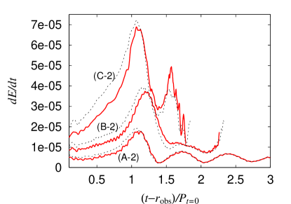
Figure 10: Luminosity of gravitational waves as functions of the retarded time for models (A-2), (B-2) and (C-2). Solid and dashed curves represent the luminosity computed at $r_{\rm obs}\approx L$ and $0.77L$, respectively. $r_{\rm obs}$ denotes the radius at which the gauge invariant variables are extracted. For $t-r_{\rm obs}\mathrel{\raise 1.29167pt\hbox{$<$}\mkern-14.0mu\lower 2.58334pt\hbox{$\sim$}}P_{t=0}$, the wavelength of gravitational waves is longer than $L$, but for $t-r_{\rm obs}\mathrel{\raise 1.29167pt\hbox{$>$}\mkern-14.0mu\lower 2.58334pt\hbox{$\sim$}}1.2P_{t=0}$, it becomes shorter than $L$ (see Fig. 9). The unit of luminosity is $c^{5}/G\approx 3.63\times 10^{59}$ erg/sec.

Table 3: Total radiated energy and angular momentum in units of their initial values. We estimated the fluxes at $r_{\rm obs}\approx L$. If we estimated them at $r_{\rm obs}\approx 0.77L$, they are overestimated by $\sim 20\%$, because of inaccurate extraction of gravitational waves in the early stages during which the gravitational wavelength is longer than $L$.

Model	$\Delta E/M_{\rm ADM0}$	$\Delta J/J_{0}$
(A-2)	0.5%	8%
(B-2)	0.6%	10%
(C-2)	0.9%	12%
(E-1)	0.3%	6%
(F-1)	0.3%	7%
(H-1)	0.6%	10%

We list the total radiated energy $\Delta E$ and angular momentum $\Delta J$ in Table III. A typical magnitude of $\Delta J/J_{0}$ is $\sim 10\%$, which is consistent with the decrease of the angular momentum $J$ computed by Eq. (54). (It was impossible to confirm the consistency of the change of $M_{\rm ADM}$ due to radiation reaction, because $M_{\rm ADM}$ varies by $\mathrel{\raise 1.29167pt\hbox{$<$}\mkern-14.0mu\lower 2.58334pt\hbox{$\sim$}}10\%$ during simulations due to numerical error; see discussion in the Appendix.) It should be noted that $\Delta J/J_{0}$ is much larger than $\Delta E/M_{\rm ADM0}$, because the approximate relation $\Delta J\sim\Delta E/\Omega$ holds, and hence

$${(\Delta J/J_{0})\over(\Delta E/M_{\rm ADM0})}\sim 10\biggl{(}{1\over q}\biggr{)}\biggl{(}{0.1\over M_{\rm ADM0}\Omega}\biggr{)},$$ (86)

where $\Omega$ here denotes a typical magnitude of the angular velocity.

During the early stages ($t\mathrel{\raise 1.29167pt\hbox{$<$}\mkern-14.0mu\lower 2.58334pt\hbox{$\sim$}}P_{t=0}$), the luminosity of gravitational waves gradually increases, reaching a peak. The peak luminosity is approximately proportional to $(M/R)_{\infty}^{5}$, as expected from the quadrupole formula. However, after the peak is reached, the behavior of the curve depends strongly on the outcome of the merger.

For model (C-2), in which a black hole is formed in a short timescale at $t\sim 2P_{t=0}$ ($t-r_{\rm obs}\sim 1.7P_{t=0}$), a sharp peak is found before the black hole is formed. This peak is likely associated with an oscillation for a short-lived transient merged object. It is likely that peaks associated with QNMs appear after this peak, and the luminosity is eventually damped. For model (B-2), a long-lived transient object emits quasi-periodic gravitational waves for a certain duration. Consequently, the luminosity remains fairly large for a longer timescale than for model (C-2).

In the simulations with models (B) and (C), the computation crashed soon after the formation of an apparent horizon, and hence it was not possible to observe gravitational waves associated with QNMs of the formed black hole. If it could be extracted, the peak associated with QNMs would appear at $(t-r_{\rm obs})/P_{t=0}\sim 2$ for model (C-2) and $\sim 2.5$ for model (B-2), before the luminosity is damped to zero.

For the case of neutron star formation [model (A-2)], the evolution of the luminosity is very different from that for the other models after the first peak is reached. In this case, the luminosity oscillates with average amplitude $dE/dt\sim 5\times 10^{-6}$ after formation of the massive neutron star. We here estimate the approximate timescale for gravitational radiation reaction.

The binding energy of the massive neutron star is approximately

$$W\sim{M^{2}\over R}=0.2M\biggl{(}{5M\over R}\biggr{)},$$ (87)

where $M$ is the gravitational mass and $R$ is a typical radius of the massive neutron star $\sim 5M$. The ratio of the kinetic energy $T$ to $W$ is expected to be between 0.1 and 0.2, so that

$$T\sim(0.02-0.04)M\biggl{(}{5M\over R}\biggr{)}.$$ (88)

Assuming that the energy luminosity remains $\sim 10^{-6}$, as indicated in Fig. 10, and that the emission timescale is approximately derived by dividing $T$ by $dE/dt$, we obtain

$$t_{\rm GW}\sim{T\over dE/dt}\mathrel{\raise 1.29167pt\hbox{$<$}\mkern-14.0mu\lower 2.58334pt\hbox{$\sim$}}0.1{\rm sec}\biggl{(}{M\over 3M_{\odot}}\biggr{)}\biggl{(}{5M\over R}\biggr{)}\biggl{(}{5\times 10^{-6}\over dE/dt}\biggr{)}.$$ (89)

Thus, within $\sim 0.1$ sec (or $\sim 50P_{t=0}$), the massive neutron star will collapse into a black hole. As argued in Ref. BSS, there are many other processes of dissipation and transport of angular momentum inside the massive neutron star, in addition to the emission of gravitational waves. However, the characteristic timescale for such processes is much longer than 1 sec. Thus, the emission timescale of gravitational waves would be shortest in this case. On the other hand, if $t_{\rm GW}$ were longer than 10 seconds, other processes, such as magnetic braking effect, could be more important than the effect of gravitational radiation.[32]

Figure 11: $\bar{h}_{+}$ and $\bar{h}_{\times}$ as functions of the retarded time for models (E-1) and (H-1).

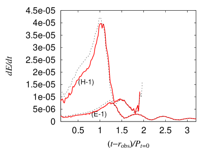
Figure 12: The same as Fig. 10 but for models (E-1) and (H-1).

All features mentioned above for $\Gamma=2.25$ are also found in gravitational waveforms for $\Gamma=2$. In Fig. 11, we display $\bar{h}_{+}$ and $\bar{h}_{\times}$ for models (E-1) and (H-1). In Fig. 12, we also display the luminosity for these models. For model (H-1), a black hole is formed, while for (E-1), a neutron star is the outcome. As in the $\Gamma=2.25$ case, this feature is well reflected in Figs. 11 and 12: Quasi-periodic oscillations are seen over a long duration for model (E-1), while for model (H-1), such oscillations are found only for a short timescale.

For model (E-1), the luminosity remains $\sim 10^{-6}$ after formation of a massive neutron star. Thus, the emission timescale of gravitational waves from a formed massive neutron star is likely shorter than 1 sec, as shown in Eq. (89). This implies that, as in the case of model (A), it eventually collapses into a black hole, due to the angular momentum dissipation through gravitational waves.

4.2.2 Gravitational wave spectra

In Fig. 13, spectra of gravitational waves are displayed for $\Gamma=2.25$ [models (A-2), (B-2) and (C-2) on the left] and for $\Gamma=2$ [models (F-1) and (H-1) on the right]. Since the computation crashed soon after formation of the black hole, the spectra of models (B-2), (C-2) and (H-1) are incomplete on the high frequency side [i.e., for $f_{\rm GW}/f_{\rm QE}\mathrel{\raise 1.29167pt\hbox{$>$}\mkern-14.0mu\lower 2.58334pt\hbox{$\sim$}}4$, where $f_{\rm QE}$ is given in Eq. (81)]. In these cases, QNMs of black holes would be excited in the last stage of black hole formation. However, as mentioned in §1, the frequency would be very high ($f_{\rm GW}>5~{}{\rm kHz}\sim 5f_{\rm QE}$). Here, we focus only on the spectra for quasi-periodic oscillations of merged objects for which $f_{\rm GW}\sim(2-3)~{}{\rm kHz}$, so that the incompleteness with regard to the spectra on the higher frequency side is not a problem. For the spectra of model (A), it should be kept in mind that the peak associated with the quasi-periodic oscillations is underestimated in Fig. 13, because quasi-periodic waves will be emitted perhaps to $t\sim 100P_{t=0}$, as indicated in Eq. (89). For all models, we should also point out that in the real spectra of the coalescing binaries, $\bar{h}_{+,\times}\propto f_{\rm GW}^{-7/6}$ for $f_{\rm GW}\mathrel{\raise 1.29167pt\hbox{$<$}\mkern-14.0mu\lower 2.58334pt\hbox{$\sim$}}f_{\rm QE}$,[37] which is not taken into account in the present results.

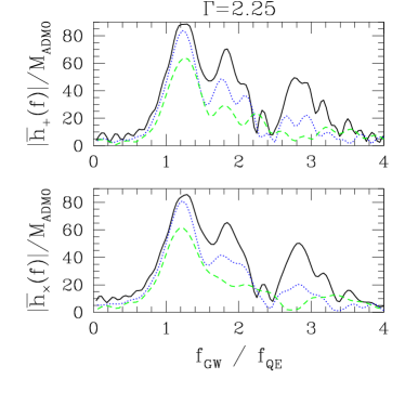
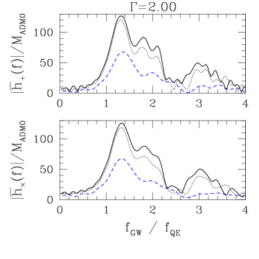
Figure 13: Fourier spectra of $\bar{h}_{+}$ and $\bar{h}_{\times}$ for models (A-2) (solid curve), (B-2) (dotted curve) and (C-2) (dashed curve) [left], and for models (E-1) (solid curve), (F-1) (dotted curve) and (H-1) (dashed curve) [right].

From Fig. 13, we find two typical frequencies of the quasi-periodic oscillation for each $\Gamma$:

$$f_{\rm QPO} \sim \left\{\begin{array}[]{ll}\displaystyle 1.8f_{\rm QE}\approx 1.7~{}{\rm kHz}\biggl{(}{2.8M_{\odot}\over M_{\rm ADM0}}\biggr{)}\biggl{(}{C_{0}\over 0.12}\biggr{)}^{3/2}&\\ \displaystyle 2.8f_{\rm QE}\approx 2.7~{}{\rm kHz}\biggl{(}{2.8M_{\odot}\over M_{\rm ADM0}}\biggr{)}\biggl{(}{C_{0}\over 0.12}\biggr{)}^{3/2}&\end{array}\right.{\rm for}~{}\Gamma=2.25,\$$ (92)

$$f_{\rm QPO} \sim \left\{\begin{array}[]{ll}\displaystyle 1.8f_{\rm QE}\approx 1.7~{}{\rm kHz}\biggl{(}{2.8M_{\odot}\over M_{\rm ADM0}}\biggr{)}\biggl{(}{C_{0}\over 0.12}\biggr{)}^{3/2}&\\ \displaystyle 3.0f_{\rm QE}\approx 2.9~{}{\rm kHz}\biggl{(}{2.8M_{\odot}\over M_{\rm ADM0}}\biggr{)}\biggl{(}{C_{0}\over 0.12}\biggr{)}^{3/2}&\end{array}\right.{\rm for}~{}\Gamma=2.\$$ (95)

This shows that the ratio of $f_{\rm QPO}$ to $f_{\rm QE}$ is not very sensitive to $(M/R)_{\infty}$. However, this ratio for higher frequencies $\sim 3f_{\rm QE}$ depends on the stiffness (or $\Gamma$) of the equations of state. The numerical results indicate that this ratio is larger for softer equations of state for a peak of higher frequency. (This fact agrees with the results of Newtonian and post Newtonian simulations. [7, 10, 12]) As pointed out in Ref. C, from the frequencies of quasi-periodic oscillations, we could constrain the stiffness of equations of state.

As explained above, the peaks of the Fourier spectra that are associated with the quasi-periodic oscillations are determined by its accumulated cycles. Hence, if we would not find a large peak, we could conclude that a black hole is formed in a short timescale after merger. This implies that even without detecting QNMs or other signals of the black hole, it is possible to obtain evidence for black hole formation. On the other hand, if we would find a large peak, we could conclude that a massive neutron star is formed, at least temporarily. The criterion for the formation of black holes depends on the compactness and stiffness of the equations of state of the merging neutron stars. Thus, this information is also useful for constraining the equations of state.

From gravitational waves emitted in the inspiraling stage with post-Newtonian templates of waveforms,[35] the masses of the two neutron stars, and hence, the total mass, will be determined.[37] As mentioned above, from the intensity of the peak of the spectra associated with quasi-periodic oscillations, we can infer the compactness (for a given stiffness of an equation of state). This combined observation could constrain the relation between the compactness and mass of neutron stars. In this way, it is likely possible to strongly constrain nuclear equations of state using observed quantities such as the intensity of the Fourier peak of quasi-periodic oscillation, the ratio of $f_{\rm QPO}$ to $f_{\rm QE}$, and the total mass of the system.

Since $f_{\rm QPO}$ is rather high, it may be difficult to detect quasi-periodic oscillation by first generation, kilometer-size laser interferometers, such as LIGO I. However, resonant-mass detectors and/or specially designed advanced interferometers, such as LIGO II, may be capable in the future to detect such high frequency gravitational waves. These detectors will provide us a wide variety of information on neutron star physics.

4.2.3 Calibrations

To assess the accuracy and robustness of our results as well as to investigate the influence of the approximate initial conditions on gravitational waveforms, we performed several test simulations.

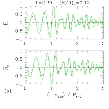
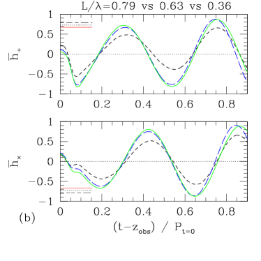
Figure 14: (a): $\bar{h}_{+}$ and $\bar{h}_{\times}$ for models (A-2) (solid curve) and (A-0) (dashed curve). (b): $\bar{h}_{+}$ and $\bar{h}_{\times}$ for models (C-3) (solid curve), (C-2) (long dashed curve) and (C-0) (dashed curve). The horizontal solid, dotted and dashed lines drawn near the vertical axis denote the theoretical amplitudes at $t=0$ computed in the 2.5, second post-Newtonian and quadrupole approximations.

As mentioned above, the numerical accuracy of the gravitational wave amplitude depends on the location of the outer boundaries $L$ and the grid spacing $\Delta x$. It is indicated that (1) smaller $L(<\lambda)$ and larger $\Delta x$ result in the underestimation of $\bar{h}_{+,\times}$ and (2) smaller $L(\ll\lambda)$ also induces spurious modulation of $\bar{h}_{+,\times}$ (by which $\bar{h}_{+,\times}$ deviate from zero systematically). However, we will show that with the typical grid size adopted in the present work ($L\mathrel{\raise 1.29167pt\hbox{$>$}\mkern-14.0mu\lower 2.58334pt\hbox{$\sim$}}0.6\lambda$), these numerical errors are sufficiently suppressed.

First, we investigate the convergence of the wave amplitude resulting when the computational domain is enlarged. In Fig. 14 (a), we compare the merger waveforms for model (A) with (293,293,147) [(A-0)] and (505,505,253) [(A-2)] grid numbers. We note that $L\sim\lambda_{\rm QP}$ for the smaller grid number and $L\sim 2\lambda_{\rm QP}$ for the large grid number, where $\lambda_{\rm QP}$ here denotes the wavelength of quasi-periodic gravitational waves emitted by a formed massive neutron star. Figure 14 (a) shows that the amplitude of gravitational waves from quasi-periodic oscillations is not sensitive to $L$. This indicates that a value of $L$ that is $\mathrel{\raise 1.29167pt\hbox{$>$}\mkern-14.0mu\lower 2.58334pt\hbox{$\sim$}}\lambda_{\rm QP}$ is sufficiently large for computing waveforms associated with quasi-periodic oscillations of a formed massive neutron star. On the other hand, it is not clear if convergence is achieved for the wave amplitude for $t\mathrel{\raise 1.29167pt\hbox{$<$}\mkern-14.0mu\lower 2.58334pt\hbox{$\sim$}}P_{t=0}$.

Table 4: Amplitudes of $\bar{h}_{+,\times}$ at $t=0$ for several levels of the post-Newtonian approximation.

Model	quadrupole	1PN	1.5PN	2PN	2.5PN
(A)	0.755	0.611	0.738	0.705	0.681
(B)	0.766	0.594	0.760	0.712	0.676
(C)	0.785	0.578	0.793	0.727	0.671
(E)	0.735	0.620	0.712	0.690	0.675
(H)	0.759	0.590	0.752	0.705	0.670

To evaluate the numerical error in the amplitude for $t\mathrel{\raise 1.29167pt\hbox{$<$}\mkern-14.0mu\lower 2.58334pt\hbox{$\sim$}}P_{t=0}$, we compare the waveforms for models (C-0), (C-2) and (C-3) in Fig. 14 (b), in which $L/\lambda_{0}=0.36$, 0.63, and 0.79, respectively. In addition to the waveforms, the amplitudes predicted from the post-Newtonian theory are shown by horizontal lines. Here, the wave amplitude of the $|m|=2$ modes (sum of $l=2$ to $l=6$ modes) for a binary of equal point mass in circular orbits can be written as

$${M_{\rm tot}v^{2}\over D}\biggl{[}1-{17\over 8}v^{2}+2\pi v^{3}-{15917\over 2880}v^{4}-{17\over 4}\pi v^{5}\biggr{]}$$ (96)

at the 2.5 post-Newtonian order,[35, 36] where $M_{\rm tot}$ is the sum of the gravitational masses of the two stars in isolation (hence $M_{\rm tot}\not=M_{\rm ADM0}$ for a finite separation, due to the existence of the binding energy between the two stars) and $v=(M_{\rm tot}\Omega_{0})^{1/3}$. We list the amplitudes of $\bar{h}_{+,\times}$ for several levels of the post-Newtonian approximation in Table IV. It is seen that the amplitude converges to $\sim 0.7$ for each model. Figure 14 (b) indicates that for model (C-0), the amplitude is underestimated by 30–40 %, but as $L$ increases, a convergence is achieved. The wave amplitudes for models (C-2) and (C-3) are nearly coincident and also agree with the 2.5 post-Newtonian amplitudes within $<10\%$ error. Thus, with these computational domains with $L\mathrel{\raise 1.29167pt\hbox{$>$}\mkern-14.0mu\lower 2.58334pt\hbox{$\sim$}}0.6\lambda_{0}$, the amplitude seems to be computed within $10\%$ error, and hence we may assume that the error on the wave amplitude calculated for models (B-2), (C-2), and (H-1), shown in Figs. 9 and 11, is less than $10\%$. This conclusion agrees with that of our recent numerical experiment on gravitational waveforms from inspiraling binary neutron stars in quasiequilibrium states.[29]

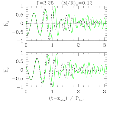
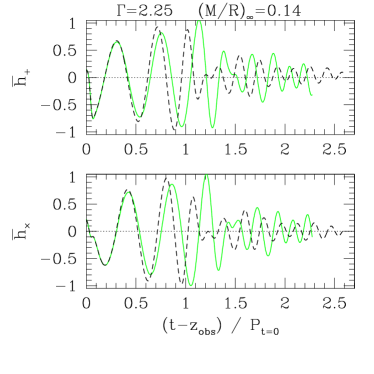
Figure 15: Left: $\bar{h}_{+}$ and $\bar{h}_{\times}$ as functions of the retarded time for models (A-2) (solid curve) and (A-3) (dashed curve). Right: The same as (a) but for (B-2) (solid curve) and (B-3) (dashed curve).

Next, we investigate the effect of the grid resolution ($\Delta x$) on gravitational waveforms. In Fig. 15, we show $\bar{h}_{+}$ and $\bar{h}_{\times}$ for models (A-2) and (A-3) and models (B-2) and (B-3) for comparison. At a glance, we find that the global properties in the waveforms are similar with regard to results for high and low resolution. However, two differences are also found : (1) since the merger starts earlier, due to larger numerical dissipation, merger waveforms start earlier for simulations with lower resolution; (2) the wave amplitude is underestimated for lower resolution. Property (2) can be understood in the following manner. In the simulation with lower resolution, the density gradient is less accurately computed. The wave amplitude becomes higher in association with the formation of higher density peaks. Thus, the lower resolution results in underestimation of the gravitational wave amplitude. [This property has been found in many Newtonian simulations using Eulerian codes; e.g., Ref. RJ.]

It is desirable to further investigate the convergence improving the resolution in order to draw definite conclusions about whether the convergence of the waveforms is fully achieved. However, it is pragmatically difficult to do this with the current computational resources, because a simulation with a large grid size, e.g., (633, 633, 317), would take a very long computational time, perhaps $\mathrel{\raise 1.29167pt\hbox{$>$}\mkern-14.0mu\lower 2.58334pt\hbox{$\sim$}}200$–250 CPU hours, which is about 1/3 of the computational time assigned to us. In the future, it will be feasible to improve the resolution using better computational resources. In addition, an adaptive mesh refinement (AMR) technique for high density regions might be necessary to save computational time and memory.[38]

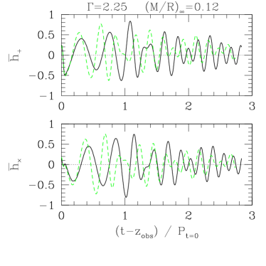
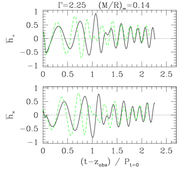
Figure 16: Left: $\bar{h}_{+}$ and $\bar{h}_{\times}$ for models (A-0) (solid curve) and (A-1) (dashed curve). Right: The same as (a) but for models (B-0) (solid curve) and (B-1) (dashed curve). The amplitude is underestimated by 30–40 % in the early stages ($t\mathrel{\raise 1.29167pt\hbox{$<$}\mkern-14.0mu\lower 2.58334pt\hbox{$\sim$}}P_{t=0}$), because the computational domain in these simulations is too small (see Figs. 9 and 14 for comparison).

Finally, we investigate the effect of an approaching velocity, which we ignored in our main simulations for $\Gamma=2.25$. In this test, we perform a simulation with a large approaching velocity as $v_{\rm app}=0.1v_{\rm orb}$ for $(M/R)_{\infty}=0.12$ [model (A-1)], and for $(M/R)_{\infty}=0.14$ [model (B-1)] with (313,313,157) grid number. For model (B-1), we also decrease the reduction factor of the angular momentum by 1% (see Table II). In Fig. 16, we show $\bar{h}_{+}$ and $\bar{h}_{\times}$ for these two cases. For comparison, we also plot the waveforms of models (A-0) and (B-0). Because of the approaching velocity, the waveforms before merger starts are very different for the two cases; the wavelength becomes short for models (A-1) and (B-1) soon after the simulations start. However, the quasi-periodic waveforms after the onset of the hydrodynamic interaction of two neutron stars are quite similar. This is because the quasi-periodic waves are associated with the fundamental oscillation modes of merged objects, which appear to depend weakly on the approaching velocity. Thus, we may conclude that the waveforms in the merger do not depend strongly on the approaching velocity, as long as $v_{\rm app}$ is not extremely large, i.e., as long as $\leq 0.1v_{\rm orb}$.

We note that $\bar{h}_{+}$ in Fig. 16 deviates from zero in the late stages for $t-z_{\rm obs}\mathrel{\raise 1.29167pt\hbox{$>$}\mkern-14.0mu\lower 2.58334pt\hbox{$\sim$}}1.5P_{t=0}$ [in particular for model (B)]. This spurious effect results from the fact that the outer boundaries are too close to the strong field zone. Indeed, this numerical effect disappears when we increased the grid number to enlarge the computational domain (compare with Fig. 9).

5 Summary

Using a new large scale supercomputer at NAOJ, we have performed fully GR simulations for the merger of equal mass binary neutron stars, particularly focusing on gravitational waveforms. Since the computational domain is much larger than that used in previous simulations, gravitational waveforms can be computed much more accurately than those reported in Refs. bina and binas. In the following, we summarize the results obtained in this paper.

The merger process and final products depend strongly on the compactness and the stiffness of the equations of state for the merging neutron stars. For binaries of less compact neutron stars, massive neutron stars are formed, at least temporarily. In contrast, black holes are formed in the merger of sufficiently compact neutron stars on a dynamical timescale. However, the formation timescale of a black hole depends strongly on the compactness of the neutron stars. The criterion regarding compactness for prompt formation of a black hole depends also on the stiffness of equations of state. For $\Gamma=2.25$ and 2, threshold values are $\sim 0.16$ and $\sim 0.14$, respectively.

The nature of the gravitational waveforms during the merger depend sensitively on the compactness (or mass) of the merging neutron stars. For mergers of less compact binaries, such as in models (A), (E) and (F), a transient massive neutron star is formed, and survives for the emission timescale of gravitational radiation, which is much longer than the dynamical timescale. Such massive neutron stars are highly nonaxisymmetric, so that quasi-periodic gravitational waves associated with nonaxisymmetric deformation are emitted. These quasi-periodic waves have typical frequencies of $\sim 2-3$ kHz, which yield Fourier peaks in the frequency domain of gravitational waves. The ratio of the peak frequency to the frequency at innermost orbits, $f_{\rm QPO}/f_{\rm QE}$, is not sensitive to the compactness, but depends on the stiffness of the equations of state. This indicates that its observation could constrain the stiffness of the equations of state.[7] It is also found that the luminosity of quasi-periodic gravitational waves is fairly large, so that a massive transient neutron star likely collapses into a black hole eventually, due to the angular momentum dissipation through gravitational radiation.

In models of slightly larger compactness, such as models (B) and (G), a transient massive object is also formed after merger sets in. This massive object is also highly nonaxisymmetric. Since the lifetime of such a transient massive object is fairly long, it causes characteristic peaks associated with the quasi-periodic oscillation in the Fourier domain of gravitational waves. However, for models with large compactness, such as models (C), (D), (H) and (I), the merged object collapses into a black hole on a dynamical timescale (i.e., on a few rotational periods of the merged objects), and hence quasi-periodic gravitational waves are excited only on a short timescale.

The intensity of the peaks in the Fourier spectra of gravitational waves associated with the nonaxisymmetric, quasi-periodic oscillations of the merged object depends on the lifetime of the transient massive object. If the transient object is long-lived, the peak becomes high, while if it collapses into a black hole in a few oscillation periods, the peaks are small. Therefore, from the intensity of the peak associated with the quasi-periodic oscillation, it may be possible to determine the object formed after the merger in future observations.

To this time, we have performed simulations focusing on binaries of two identical neutron stars. Although all the binary neutron stars observed so far are composed of neutron stars of two nearly identical masses,[39] it seems that there is no fundamental reason for the production of such symmetric systems. In the merger of two neutron stars of unequal mass, the merger process would be different from that for identical neutron stars. Since a less massive star is less compact, it is likely to be tidally disrupted before the dynamical instability of the orbital motion sets in. In this case, the tidally disrupted star could form accretion disks around the more massive companion. Sufficient accretion to the massive companion is likely to trigger gravitational collapse and the formation of a black hole. As a result, a system consisting of a black hole surrounded by accretion disks might be formed. Associated with the change of the merger process, gravitational waveforms would be modified.[40] To survey possible outcomes in the merger of binary neutron stars, it is obviously necessary to perform simulations for two neutron stars of unequal mass.

It is also desirable to improve the implementation of the initial conditions. In simulations carried out to this time, we have used quasiequilibrium states of a conformally flat three-metric as the initial conditions for simplicity. The conformal flatness approximation becomes a source of a certain systematic error when attempting to obtain realistic quasiequilibrium states. As a result, this approximation introduces a systematic error on the initial conditions and subsequent merger simulation. Since the magnitude of the ignored terms in the conformal flatness approximation seems to be small, we expect that this effect is not very serious. However, this conclusion is not entirely certain. To rule out this problem, it is necessary to perform simulations using more realistic quasiequilibrium states of generic three geometries as initial conditions.[41]

In addition, there are technical issues requiring improvement. As discussed above and in the Appendix, black hole forming region does not have good resolution in our current computation. Obviously, it is necessary to improve the resolution around the black hole forming region. Since we have to prepare a large computational domain $L$, which is at least equal to the wavelength of gravitational waves, using restricted computational speed and memory, it is desirable to develop numerical techniques such as the AMR technique or nested grid technique to overcome this problem. This is also an issue to be resolved in the future.

Acknowledgments

Numerical computations were performed on the FACOM VPP 5000 machines at the data processing center of NAOJ. This work was in part supported by a Grant-in-Aid (No. 13740143) of the Japanese Ministry of Education, Science, Sports, Culture, and Technology and also in part by NSF Grant PHY00-71044.

Appendix A Accuracy

We have monitored the degree of violation of the Hamiltonian constraint, conservation of the baryon rest-mass, ADM mass and angular momentum during numerical simulation.

We have found that $f_{\psi}$ is less than 0.1 for a region in which $\rho$ is larger than $\sim 10^{-3}\rho_{\rm max}$, where $\rho_{\rm max}$ is the maximum value of $\rho$. For a less dense region, $f_{\psi}$ is often $O(0.1)$, because low density regions are not well resolved in the finite differencing scheme we used for the hydrodynamic equations. When the merged object starts collapsing, $f_{\psi}$ increases to $O(0.1)$, even in a high density region. This indicates that the resolution in the black hole forming region is not very good either.

The baryon rest-mass was found to be conserved within the truncation error in all computations. This is because no mass is ejected outside the computational domain, which is wide enough.

In the case of massive neutron star formation, the ADM mass is conserved within 10% error throughout the simulation. At the last moment, at which excessive numerical error seems to accumulate, the simulation crashes, and the error of the ADM mass suddenly diverges, as shown in Fig. 17. Such a crash took place typically at some time in the range $t=700$ – $900M_{\rm ADM}$ (see §4). In the case of black hole formation, the ADM mass is conserved within 10% error until the merged object starts collapsing into a black hole. The error systematically increases whenever the lapse at the center approaches to zero, and the error in the conservation of the ADM mass is typically $\sim 20\%$ at the time of the formation of the apparent horizon (see Fig. 17). After this formation, the error rapidly increases to $O(1)$, and the computation crashes, at which time the error is of order unity. The main source of the error in the ADM mass appears to be the volume integral of $\tilde{R}_{k}^{~{}k}$, because it includes the second spatial derivative of $\tilde{\gamma}_{ij}$, and hence loses accuracy easily whenever $\tilde{\gamma}_{ij}$ has a steep gradient.

The angular momentum is conserved within $\sim 5\%$ error throughout the simulation in the case of massive neutron star formation, as discussed in §4 (except for the last moment, at which excessive numerical error accumulates). For black hole formation cases, the angular momentum is conserved within $\sim 5\%$ error until the merged object starts collapsing. The error increases when the lapse at the center approaches to zero. The error for conservation in the angular momentum is typically $\sim 10\%$ at the time of the formation of the apparent horizon. After the formation, the error increases to $O(1)$.

Figure 17: Evolution of $M_{\rm ADM}$ and $J$ as functions of $t/P_{t=0}$ for models (A-2) (dashed curve), (B-2) (long-dashed curve) and (C-2) (solid curve). An apparent horizon is formed at $t/P_{t=0}\approx 2.5$ for (B-2) and $t/P_{t=0}\approx 2$ for (C-2). We do not add loss due to gravitational waves to $M_{\rm ADM}$ and $J$.

The divergence of the numerical error after formation of the apparent horizon is likely due either to the lack of numerical resolution around black hole forming region or to the inappropriate choice of the spatial gauge. However, at present it is not clear to us whether one of these is the actual source.

References

-
[1]
R. A. Hulse and J. H. Taylor, Astrophys. J. 201
(1975), L55.
J. H. Taylor and J. M. Weisberg, Astrophys. J. 345 (1989), 434. -
[2]
V. Kalogera, R. Narayan, D. N. Spergel and J. H. Taylor,
astro-ph/0012038: See also
E. S. Phinney, Astrophys. J. 380 (1991), L17:
R. Narayan, T. Piran and A. Shemi, Astrophys. J. 379 (1991), L17. -
[3]
For example,
K. S. Thorne, in Proceeding of Snowmass
95 Summer Study on Particle and Nuclear Astrophysics and
Cosmology, eds. E. W. Kolb and R. Peccei (World Scientific,
Singapore, 1995), p. 398, and references therein.
M. Ando et al. (the TAMA collaboration), Phys. Rev. Lett. 86 (2001), 3950. -
[4]
E. W. Leaver, Proc. R. Soc. London A402 (1985), 285.
T. Nakamura, K. Oohara and Y. Kojima, Prog. Theor. Phys. Suppl. No. 90 (1987), 1. - [5] K. Uryū, M. Shibata and Y. Eriguchi, Phys. Rev. D 62 (2000), 104015.
- [6] F. Rasio and S. L. Shapiro, Astrophys. J. 401 (1992), 226; ibid 432 (1994), 242.
- [7] X. Zang, J. M. Centrella and S. L. W. McMillan, Phys. Rev. D 50 (1994), 6247; ibid 54 (1996), 7261.
- [8] K. Oohara, T. Nakamura and M. Shibata, Prog. Theor. Phys. Suppl. No. 128 (1997), 183.
- [9] M. Ruffert, H.-Th. Janka and G. Schäfer, Astron. Astrophys. 311 (1996), 532.
- [10] J. A. Faber and F. A. Rasio, Phys. Rev. D 62 (2000), 064012; ibid 63 (2001), 044012.
- [11] S. Ayal, T. Piran, R. Oechslin, M. B. Davies and S. Rosswog, Astrophys. J. 550 (2001), 846.
- [12] R. Oechslin, S. Rosswog and F. Thielmann, gr-qc/0111005.
- [13] M. Shibata and K. Uryū, Phys. Rev. D 61 (2000), 064001.
-
[14]
M. Shibata and K. Uryū,
in Proceedings of
Gravitational Waves: A Challenge to Theoretical Astrophysics, eds.
V. Ferrari, J. C. Miller and L. Rezzolla
(The Abdus Salam ICTP Publications, 2001), p. 137.
in Proceedings of 20th Texas Symposium on Relativistic Astrophysics, eds. J. C. Wheeler and H. Martel (AIP conference proceedings 586, 2001), p. 717 (astro-ph/0104409). - [15] A. Buonanno and Y. Chen, private communication.
- [16] M. Shibata, Phys. Rev. D 60 (1999), 104502.
-
[17]
K. Oohara and T. Nakamura, Prog. Theor. Phys. Suppl. No. 136
(1999), 270.
W.-M. Suen, Prog. Theor. Phys. Suppl. No. 136 (1999), 251.
J. Font et al., gr-qc/0110047. - [18] M. Shibata and T. Nakamura, Phys. Rev. D 52 (1995), 5428.
- [19] M. Shibata, Prog. Theor. Phys. 101 (1999), 1199.
- [20] e.g., S. L. Shapiro and S. A. Teukolsky, Black Holes, White Dwarfs, and Neutron Stars, Wiley Interscience (New York, 1983).
- [21] L. Smarr and J. W. York, Phys. Rev. D 17 (1978), 1945.
-
[22]
M. Shibata, T. W. Baumgarte, and S. L. Shapiro,
Phys. Rev. D 61 (2000), 044012.
M. Shibata, T. W. Baumgarte, and S. L. Shapiro, Astrophys. J. 542 (2000), 453. - [23] V. Moncrief, Ann. of Phys. 88 (1974), 323.
-
[24]
M. Shibata, Phys. Rev. D 58 (1998), 024012.
S. A. Teukolsky, Astrophys. J. 504 (1998), 442. See also,
S. Bonazzola, E. Gourgoulhon and J.-A. Marck, Phys. Rev. D 56 (1997), 7740.
H. Asada, Phys. Rev. D 57 (1998), 7292. -
[25]
K. Uryū and Y. Eriguchi, Phys. Rev. D 61 (2000), 124023.
See also Ref. \citenGBM for another method. - [26] E. Gourgoulhon et al., Phys. Rev. D 63 (2001), 064029.
- [27] J. W. York, Jr., in Sources of Gravitational Radiation, ed. L. L. Smarr (Cambridge University Press, 1979), p. 83.
- [28] J. R. Wilson and G. J. Mathews, Phys. Rev. Lett. 75 (1995), 4161.
- [29] M. Shibata and K. Uryū, Phys. Rev. D 64 (2001), 104017.
-
[30]
N. Bishop et al., Phys. Rev. Lett. 76 (1996), 4303.
A. M. Abrahams et al., Phys. Rev. Lett. 80 (1998), 1812.
L. Rezzolla et al., Phys. Rev. D 59 (1999), 064001. - [31] M. Shibata, Phys. Rev. D 55 (1997), 2002: M. Shibata and K. Uryū, Phys. Rev. D 62 (2000), 087501.
- [32] T. W. Baumgarte, S. L. Shapiro, and M. Shibata, Astrophys. J. Lett. 528 (2000), L29.
- [33] For example, M. Alcubierre et al., Phys. Rev. D 64 (2001), 061501.
-
[34]
J. Baker, M. Campanelli and C. Lousto, gr-qc/0104063.
J. Baker et al., Phys. Rev. Lett. 87 (2001), 121103, and references cited therein. - [35] L. Blanchet, B. R. Iyer, C. M. Will and A. G. Wiseman, Class. Quant. Grav. 13 (1996), 575.
- [36] L. Blanchet, Phys. Rev. D 51 (1995), 2559.
-
[37]
C. Cutler and E. E. Flanagan, Phys. Rev. D 49
(1994), 2658.
E. Poisson and C. M. Will, ibid 52 (1995), 848. - [38] M. Berger and J. Oliger, J. Comp. Phys. 53 (1984), 484.
- [39] E. S. Phinney and S. R. Kulkarni, Annu. Rev. Astron. Astrophys. 32 (1994), 591.
- [40] T. Nakamura and K. Oohara, Prog. Theor. Phys. 86 (1991), 73.
- [41] K. Uryū and M. Shibata, in preparation.