Global General Relativistic MHD Simulation of a Tilted Black-Hole Accretion Disk

Abstract

This paper presents a continuation of our efforts to numerically study accretion disks that are misaligned (tilted) with respect to the rotation axis of a Kerr black hole. Here we present results of a global numerical simulation which fully incorporates the effects of the black hole spacetime as well as magnetorotational turbulence that is the primary source of angular momentum transport in the flow. This simulation shows dramatic differences from comparable simulations of untilted disks. Accretion onto the hole occurs predominantly through two opposing plunging streams that start from high latitudes with respect to both the black-hole and disk midplanes. This is due to the aspherical nature of the gravitational spacetime around the rotating black hole. These plunging streams start from a larger radius than would be expected for an untilted disk. In this regard the tilted black hole effectively acts like an untilted black hole of lesser spin. Throughout the duration of the simulation, the main body of the disk remains tilted with respect to the symmetry plane of the black hole; thus there is no indication of a Bardeen-Petterson effect in the disk at large. The torque of the black hole instead principally causes a global precession of the main disk body. In this simulation the precession has a frequency of $3(M_{\odot}/M)$ Hz, a value consistent with many observed low-frequency quasi-periodic oscillations. However, this value is strongly dependent on the size of the disk, so this frequency may be expected to vary over a large range.

1 Introduction

Black-hole accretion has long been postulated to power the energetic emissions seen from quasars, active galactic nuclei (AGN), and many galactic X-ray sources; there is now ample observational evidence to support such claims (e.g. Krolik, 1999; McClintock & Remillard, 2005). Black-hole accretion flows are also of interest as laboratories to test predictions of general relativity. However, the nature of such flows is complex, involving time-dependent, multi-dimensional dynamics with generically little symmetry. Hence numerical simulations play an integral role in advancing our understanding.

Many simulations of black-hole accretion flows have been carried out over the past three decades, both in the hydrodynamic (e.g. Wilson, 1972; Hawley et al., 1984; Hawley, 1991) and magnetohydrodynamic (MHD) (e.g. Koide et al., 1999; Gammie et al., 2003; De Villiers & Hawley, 2003b) regimes. A common assumption in nearly all of the work to date has been that the symmetry plane of the central black hole is aligned with the midplane of the accretion flow, at least in some averaged sense. However, there is compelling observational evidence in several black-hole X-ray binaries (BHBs), e.g. GRO J1655-40 (Orosz & Bailyn, 1997) and XTE J1550-564 (Hannikainen et al., 2001; Orosz et al., 2002), and AGN, e.g. NGC 3079 (Kondratko et al., 2005), NGC 1068 (Caproni et al., 2006), and NGC 4258 (Caproni et al., 2007), suggesting that misaligned (or tilted) black holes may be common (see also Maccarone, 2002). This claim relies on the observation of relativistic bipolar jets (thought to be aligned with the spin axis of the black hole) that are not perpendicular to the plane of the accretion disk observed at large scales.

There are also compelling theoretical arguments that many black holes should be tilted. First, the formation avenues for many black-hole - disk systems favor, or at least allow for, a tilted configuration (Fragile et al., 2001). In stellar mass binaries, the orientation of the outer disk is fixed by the binary orbit, whereas the orientation of the black hole is determined by how it became part of the system, whether through a supernova explosion or multi-body interaction. If the black hole formed from a member of a preexisting binary through a supernova, then the black hole could be tilted if the explosion were asymmetric. If the black hole joined the binary through multi-body interactions, such as binary capture or replacement, then there would have been no preexisting symmetry, so the resulting system would nearly always harbor a tilted black hole. This same argument can be extended to AGN in which merger events reorient the central black hole or its fuel supply and result in repeated tilted configurations.

If an accretion disk is misaligned or tilted, it will be subject to Lense-Thirring precession. For an ideal test particle in a slightly tilted orbit at a radius $r$ around a black hole of mass $M$ and specific angular momentum $a$, this precession occurs at an angular frequency $\Omega_{\rm LT}\approx 2aM/r^{3}$. Close to the black hole, this is comparable to the orbital angular frequency $\Omega=(M/r^{3})^{1/2}/[1+a(M/r^{3})^{1/2}]\approx\Omega_{\rm Kep}$. However, because of its strong radial dependence, Lense-Thirring precession becomes much weaker far from the hole. Therefore, a disk will experience a differential precession that will tend to twist and warp it.

A warping disturbance can be communicated through a disk in either a diffusive or wave-like manner. In the diffusive case, the warping is limited by secular (i.e. “viscous”) responses within the disk. In such a case, Lense-Thirring precession is expected to dominate out to a unique, nearly constant transition radius (Bardeen & Petterson, 1975; Kumar & Pringle, 1985), inside of which the disk is expected to be flat and aligned with the black-hole midplane, and outside of which the disk is also expected to be flat but in a plane determined by the angular momentum vector of the gas reservoir. This is what we term a “Bardeen-Petterson” configuration. Interestingly, data for the two black-hole X-ray binaries previously mentioned are best fit by disk components with inclinations that differ from their binary measurements. The best-fit inclinations are more consistent with inclination constraints derived from the radio jets (Davis et al., 2006), possibly suggesting Bardeen-Petterson configurations. Caproni et al. (2006) also claim that the observations of NGC 1068 are consistent with the predictions of the Bardeen-Petterson effect. Confirmation could come through observations of relativistically broadened reflection features (Fragile et al., 2005).

The Bardeen-Petterson result is expected to apply for Keplerian disks whenever the dimensionless stress parameter $\alpha$ (Shakura & Sunyaev, 1973) is larger than the ratio of the disk semi-thickness $H$ to the radius $r$ at all radii. Given that $\alpha$ is usually considered to be significantly less than one, this implies very geometrically “thin” disks. Unfortunately, current computational limitations prevent us from conducting global simulations of disks that are this thin. On the other hand, the Bardeen-Petterson regime may not be that common in real disks. Neglecting relativistic correction factors, the innermost, radiation pressure and electron scattering dominated portions of radiatively efficient accretion disks satisfy

$$\frac{H}{r}\sim\varepsilon^{-1}\left(\frac{L}{L_{\rm Edd}}\right)\left(\frac{r}{r_{G}}\right)^{-1},$$ (1)

where $\varepsilon\sim 0.1$ is the radiative efficiency, $L/L_{\rm Edd}$ is the luminosity in units of Eddington, and $r_{G}=GM/c^{2}$ is the gravitational radius. Note that equation (1) is independent of whether the stress is chosen to be proportional to gas pressure, radiation pressure, or some combination of the two. We therefore conclude that the Bardeen-Petterson regime will be relevant in radiatively efficient disks near the black hole only for very small Eddington ratios $L/L_{\rm Edd}\lesssim\alpha\varepsilon<<1$. Moreover, radiatively less efficient, geometrically slim and thick flows will clearly not be in the Bardeen-Petterson regime.

Global simulations of tilted disks that have $H/r>\alpha$ are computationally feasible. In this regime Lense-Thirring precession is expected to produce warps that propagate in a wave-like manner (Papaloizou & Lin, 1995). In Fragile & Anninos (2005) we presented results from the first fully general relativistic three-dimensional hydrodynamic numerical studies of tilted thick-disk accretion onto rapidly rotating (Kerr) black holes. We found that, although Lense-Thirring precession did cause the disk to warp, the warping only occurred inside a radius in the disk at which the precession time became comparable to other dynamical timescales, primarily the azimuthal sound-crossing time. After the differential warping ended and the evolution became quasi-static, the disks underwent near solid-body precession at rates consistent with some low-frequency quasi-periodic oscillations (QPOs).

In this paper we extend the results of Fragile & Anninos (2005) to include magnetic fields. The inclusion of magnetic fields is important because it is now widely believed that local stresses within black-hole accretion disks are generated by turbulence that results from the magnetorotational instability (MRI; Balbus & Hawley, 1991). Here we report on our first global general relativistic MHD (GRMHD) simulation of a tilted accretion disk around a moderately rapidly rotating black hole ($a/M=0.9$). The simulation is initialized starting from the analytic solution for an axisymmetric torus around a rotating black hole. A weak poloidal magnetic field is added to the torus to seed the MRI. After the torus is initialized, the black hole is tilted by an angle $\beta_{0}=15^{\circ}$ relative to the disk through a transformation of the metric. The system is then allowed to evolve. This paper reports the results as follows: In §2 we describe the numerical procedures used in this GRMHD simulation. In §3 we present the results of this simulation. In §4 we summarize our findings and draw conclusions.

2 Numerical Methods

This work is carried out using the Cosmos++ astrophysical magnetohydrodynamics code (Anninos et al., 2005). Similar to our predecessor code Cosmos (Anninos & Fragile, 2003), Cosmos++ includes several schemes for solving the GRMHD equations. The fluid equations can be solved using a traditional artificial viscosity scheme, non-oscillatory central difference methods, or a new hybrid dual energy (internal and total) method. For this work, we use the artificial viscosity formulation, mainly because of its speed and robustness. With the magnetic fields we solve the induction equation in an advection-split form and apply a hyperbolic divergence cleanser to maintain an approximately divergence-free magnetic field. For clarity and notation sake, we present the full evolution equations for mass, internal energy, momentum, and magnetic induction as solved in this work. Throughout this paper we use units where $G=c=1$ and the metric signature is ($-$,$+$,$+$,$+$). We use the standard notation in which four- and three-dimensional tensor quantities are represented by Greek and Latin indices, respectively.

The evolution equations are

$$\partial_{t}D+\partial_{i}(DV^{i}) = 0~{},$$ (2)

$$\partial_{t}E+\partial_{i}(EV^{i}) = -P\partial_{t}W-\left(P+Q\right)\partial_{i}(WV^{i})~{},$$ (3)

$$\partial_{t}S_{j}+\partial_{i}(S_{j}V^{i}) = \frac{1}{4\pi}\partial_{t}(\sqrt{-g}B_{j}B^{0})+\frac{1}{4\pi}\partial_{i}(\sqrt{-g}B_{j}B^{i})$$ (4)

$${}+\left(\frac{S^{\mu}S^{\nu}}{2S^{0}}-\frac{\sqrt{-g}}{8\pi}B^{\mu}B^{\nu}\right)\partial_{j}g_{\mu\nu}-\sqrt{-g}~{}\partial_{j}\left(P+P_{B}+Q\right)~{},$$

$$\partial_{t}\mathcal{B}^{j}+\partial_{i}(\mathcal{B}^{j}V^{i}) = \mathcal{B}^{i}\partial_{i}V^{j}+g^{ij}~{}\partial_{i}\psi~{},$$ (5)

$$\partial_{t}\psi+c_{h}^{2}\partial_{i}\mathcal{B}^{i} = -\frac{c_{h}^{2}}{c_{p}^{2}}\psi~{},$$ (6)

where $g_{\mu\nu}$ is the 4-metric, $g$ is the 4-metric determinant, $W=\sqrt{-g}u^{0}$ is the relativistic boost factor, $D=W\rho$ is the generalized fluid density, $V^{i}=u^{i}/u^{0}$ is the transport velocity, $u^{\mu}=g^{\mu\nu}u_{\nu}$ is the fluid 4-velocity, $S_{\mu}=W(\rho h+2P_{B})u_{\mu}$ is the covariant momentum density, $E=We=W\rho\epsilon$ is the generalized internal energy density, $P$ is the fluid pressure, $Q$ is the artificial viscosity used for shock capturing, and $c_{h}$ and $c_{p}$ are coefficients to determine the strength of the hyperbolic and parabolic pieces of the divergence cleanser. There are two representations of the magnetic field in these equations: $B^{\mu}$ is the rest frame magnetic induction used in defining the stress tensor

$$T^{\mu\nu}=\left(\rho h+2P_{B}\right)u^{\mu}u^{\nu}+\left(P+P_{B}\right)g^{\mu\nu}-\frac{1}{4\pi}B^{\mu}B^{\nu}$$ (7)

and

$$\mathcal{B}^{\mu}=W(B^{\mu}-B^{0}V^{\mu})$$ (8)

is the divergence-free ($\partial\mathcal{B}^{i}/\partial x^{i}=0$), spatial ($\mathcal{B}^{0}=0$) representation of the field. The time component of the magnetic field $B^{0}$ is recovered from the orthogonality condition $B^{\mu}u_{\mu}=0$

$$B^{0}=-\frac{W}{g}\left(g_{0i}\mathcal{B}^{i}+g_{ij}\mathcal{B}^{j}V^{i}\right)~{}.$$ (9)

The relativistic enthalpy is

$$h=1+\frac{\Gamma P}{(\Gamma-1)\rho}+\frac{Q}{\rho}~{},$$ (10)

where we have assumed an equation of state of the form $P=(\Gamma-1)\rho\epsilon$. Finally, $P_{B}=||B||^{2}/8\pi=g_{\mu\nu}B^{\mu}B^{\nu}/8\pi$ is the magnetic pressure. We use the scalar $Q$ from Anninos et al. (2005) with $k_{q}=2.0$ and $k_{l}=0.3$. We fix the divergence cleanser coefficients to be $c_{h}=c_{\rm cfl}\Delta x_{\rm min}/\Delta t$ and $c_{p}^{2}=c_{h}$, where $c_{\rm cfl}=0.7$ is the Courant coefficient, $\Delta x_{\rm min}$ is the minimum covariant zone length, and $\Delta t$ is the evolution timestep. For simplicity, we hold the timestep fixed at $\Delta t=c_{\rm cfl}\Delta x_{\rm min}$ throughout the simulation.

These GRMHD equations are evolved in a “tilted” Kerr-Schild polar coordinate system $({t},{r},{\vartheta},{\varphi})$. This coordinate system is related to the usual (untilted) Kerr-Schild coordinates $({t},{r},{\theta},{\phi})$ through a simple rotation about the ${y}$-axis by an angle $\beta_{0}$, such that

$$\left(\begin{array}[]{c}\sin{{\vartheta}}\cos{{\varphi}}\\ \sin{{\vartheta}}\sin{{\varphi}}\\ \cos{{\vartheta}}\end{array}\right)=\left(\begin{array}[]{ccc}\cos{\beta_{0}}&0&-\sin{\beta_{0}}\\ 0&1&0\\ \sin{\beta_{0}}&0&\cos{\beta_{0}}\end{array}\right)\left(\begin{array}[]{c}\sin{{\theta}}\cos{{\phi}}\\ \sin{{\theta}}\sin{{\phi}}\\ \cos{{\theta}}\end{array}\right)~{}.$$ (11)

The full tilted metric terms are provided in Fragile & Anninos (2005) [see also Fragile & Anninos (2007)]. The computational advantages of the “horizon-adapted” Kerr-Schild form of the Kerr metric were first described in Papadopoulos & Font (1998) and Font et al. (1998). The primary advantage is that, unlike Boyer-Lindquist coordinates, there are no singularities in the metric terms at the event horizon, so the computational mesh can extend into the hole’s interior. In principle, this should keep the inner boundary causally disconnected from the flow, although numerically there is still some communication.

The simulation is carried out on a spherical polar mesh with nested resolution layers. The base grid contains $32^{3}$ mesh zones and covers the full $4\pi$ steradians. Varying levels of refinement are added on top of this base layer; each refinement level doubles the resolution relative to the previous layer. The main simulation, referenced as Model 915h, has two levels of refinement, thus achieving a peak resolution equivalent to a $128^{3}$ simulation. For comparison we also discuss results from an equivalent untilted simulation (Model 90h) with the same resolution. As an argument that our results are reasonably well converged, we also include results from two other tilted simulations: one with a single refinement layer and an equivalent resolution of $64^{3}$ (Model 915m) and another that starts from a base grid of $24\times 24\times 32$ and adds three layers of refinement for an equivalent resolution of $192\times 192\times 256$ (Model 915vh). The evolution times for these simulations differ as described below. In all cases, the full refinement covers the region $r_{\rm min}\leq r\leq r_{\rm max}$, $0.075\pi=\vartheta_{1}\leq\vartheta\leq\vartheta_{2}=0.925\pi$, $0\leq\varphi\leq 2\pi$, where $r_{\rm min}=0.98r_{\rm BH}=1.41r_{G}$ and $r_{\rm max}=120r_{G}$ are the inner and outer boundaries of the grid, respectively, and $r_{\rm BH}=1.43r_{G}$ is the black-hole horizon radius. The primary motivation for using a nested grid is to allow us to maintain a reasonable Courant-limited timestep without sacrificing any spatial resolution within the disk nor completely excluding the region near the pole. The gain in computational efficiency is significant since, for a polar mesh, the timestep scales as $\Delta t\sim r_{\rm min}\sin\vartheta_{\rm min}\Delta\varphi$. By underresolving the polar region, we gain by increasing both $\vartheta_{\rm min}$ and $\Delta\varphi$. With 2 levels of refinement, we are able to use a timestep that is a factor of 11.8 larger than what we could use if our most refined layer extended all the way to the pole. The main drawback of this approach is that we are unable to resolve the region in which jets are expected to form.

In the radial direction we use a logarithmic coordinate of the form $\eta\equiv 1.0+\ln(r/r_{\rm BH})$. The spatial resolution near the black-hole horizon is $\Delta r\approx 0.05r_{G}$; near the initial pressure maximum of the torus, the resolution is $\Delta r\approx 0.5r_{G}$. Both are considerably smaller than the initial characteristic MRI wavelength $\lambda_{\mathrm{MRI}}\equiv 2\pi v_{\mathrm{A}}/\Omega\approx 2.5r_{G}$. This also gives us a large number of zones inside the plunging region. In the angular direction, in addition to the nested grids, we use a concentrated latitude coordinate $x_{2}$ of the form $\vartheta=x_{2}+\frac{1}{2}(1-h)\sin(2x_{2})$ with $h=0.5$, which concentrates resolution toward the midplane of the disk. As a result $r_{\rm center}\Delta\vartheta=0.3r_{G}$ near the midplane while it is a factor of $\sim 3$ larger for the fully refined zones near the pole. The grid used in Models 915h and 90h is shown in Figure 1.

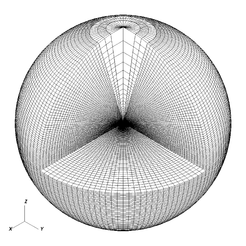
Figure 1: Plot of the grid geometry used for the main simulation (Model 915h). The initial torus is aligned in the symmetry plane of the grid, while the black hole is not.

Since we cover the full $4\pi$ steradians, the only “external” boundaries are the inner and outer radial boundaries, where we apply outflow conditions: Fluid variables are set the same in the external boundary zone as in the neighboring internal zone, except for velocity, which is chosen to satisfy

$$V^{r}_{\mathrm{ext}}=\left\{\begin{array}[]{cc}V^{r}_{\mathrm{int}}&\mathrm{when~{}}V^{r}\mathrm{~{}points~{}off~{}the~{}grid}~{},\\ -V^{r}_{\mathrm{int}}&\mathrm{when~{}}V^{r}\mathrm{~{}points~{}onto~{}the~{}grid}~{}.\end{array}\right.$$ (12)

In the azimuthal direction we apply periodic boundaries at $\varphi=0$ and $2\pi$. Since Cosmos++ is a zone-centered code, we do not have to treat the pole ($\vartheta=0$ or $\pi$) directly. Instead unboosted scalar quantities, such as the gas pressure $P$, in the “ghost” zones across the pole are filled with real data from the corresponding zone located $180^{\circ}$ away in azimuth. Unboosted vector quantities, such as velocity $V^{i}$, are similarly filled with data from appropriate real zones, albeit with the signs reversed for the $\vartheta$ and $\varphi$ components to maintain a consistent sense of coordinate direction across the pole. Boosted quantities, since they contain the metric determinant $\sqrt{-g}$, are reflected across the pole so they extrapolate to zero there. This treatment differs from the pure reflecting boundaries used in other works (e.g. De Villiers et al., 2003; McKinney, 2006) in its treatment of the unboosted variables. For untilted black holes the difference is relatively minor. However, for tilted black holes, our approach makes the pole more transparent to the fluid.

We initialize these simulations starting from the analytic solution for an axisymmetric torus around a rotating black hole (Chakrabarti, 1985). To provide a link with an untilted model already in the literature, we start with identical torus conditions as model KDP of De Villiers et al. (2003), which is the relativistic analog of model GT4 of Hawley (2000). In our initialization, the torus is defined by: the black-hole spacetime, specifically the spin of the black hole; the inner radius of the torus $r_{in}$; the radius of the pressure maximum of the torus $r_{\rm center}$; and the power-law exponent $q$ used in defining the specific angular momentum distribution,

$$\ell=-u_{\phi}/u_{t}=k\Lambda^{2-q}~{}.$$ (13)

As in model KDP, $a/M=0.9$, $r_{\rm in}=15r_{G}$, $r_{\rm center}=25r_{G}$, and $q=1.68$. Knowledge of $r_{\rm center}$ leads directly to a determination of $\ell_{\rm center}$ by setting it equal to the geodesic value at that radius. The numerical value of $k$ comes directly from the choice of $q$ and the determination of $\Lambda_{\rm center}$, where

$$\frac{1}{\Lambda^{2}}=-\frac{g_{t\phi}+\ell g_{tt}}{\ell g_{\phi\phi}+\ell^{2}g_{t\phi}}~{}.$$ (14)

Finally, having chosen $r_{in}$ we can obtain $u_{in}=u_{t}(r_{in})$, the surface binding energy of the torus, from $u_{t}^{-2}=g^{tt}-2\ell g^{t\phi}+\ell^{2}g^{\phi\phi}$.

The solution of the torus variables can now be specified. The internal energy of the torus is (De Villiers et al., 2003)

$$\epsilon(r,\theta)=\frac{1}{\Gamma}\left[\frac{u_{in}f(\ell_{in})}{u_{t}(r,\theta)f(\ell(r,\theta))}\right]~{},$$ (15)

where $\ell_{in}=\ell(r_{in})$ is the specific angular momentum of the fluid at the surface and

$$f(\ell)=\left|1-k^{2/n}\ell^{\alpha}\right|^{1/\alpha}~{},$$ (16)

where $n=2-q$ and $\alpha=(2n-2)/n$. Assuming an isentropic equation of state $P=\rho\epsilon(\Gamma-1)=\kappa\rho^{\Gamma}$, the density is given by $\rho=\left[\epsilon(\Gamma-1)/\kappa\right]^{1/(\Gamma-1)}$. As in model KDP, we take $\Gamma=5/3$ and $\kappa=0.01$ (arbitrary units). Finally, the angular velocity of the fluid is specified by

$$\Omega=V^{\phi}=-\frac{g_{t\phi}+\ell g_{tt}}{g_{\phi\phi}+\ell g_{t\phi}}~{}.$$ (17)

The dependence of $\Lambda$ on $\ell$ in equation (14) for Kerr black holes means that the solution requires an iterative procedure. However, we can get an approximate solution by taking the Schwarzschild form (i.e. ignoring $g_{t\phi}$)

$$\Lambda^{2}=-\frac{g_{\phi\phi}}{g_{tt}}~{}.$$ (18)

The error introduced by doing so is small and only affects the initial torus configuration, which will already be unstable to the MRI due to the seed magnetic fields being added. Thus, this slightly simplified treatment has no real consequence for the evolution. We note that the same procedure is followed in De Villiers et al. (2003).

Once the torus is constructed, it is seeded with a weak magnetic field in the form of poloidal loops along the isobaric contours within the torus. The initial magnetic field vector potential is (De Villiers & Hawley, 2003a)

$$A_{\varphi}=\left\{\begin{array}[]{ccc}b(\rho-\rho_{\rm cut})&\mathrm{for}&\rho\geq\rho_{\rm cut}~{},\\ 0&\mathrm{for}&\rho<\rho_{\rm cut}~{}.\end{array}\right.$$ (19)

The non-zero spatial magnetic field components are then $\mathcal{B}^{r}=-\partial_{\vartheta}A_{\varphi}$ and $\mathcal{B}^{\vartheta}=\partial_{r}A_{\varphi}$. The parameter $\rho_{\rm cut}=0.5*\rho_{\rm max,0}$ is used to keep the field a suitable distance inside the surface of the torus, where $\rho_{\rm max,0}$ is the initial density maximum within the torus. Using the constant $b$ in equation (19), the field is normalized such that initially $\beta_{\rm mag}=P/P_{B}\geq\beta_{\rm mag,0}=10$ throughout the torus. This initialization is slightly different than De Villiers & Hawley (2003b), who use a volume integrated $\beta_{\rm mag}$ to set the field strength; the difference is such that $\beta_{\rm mag,0}=100$ in their work is roughly comparable to $\beta_{\rm mag,0}=10$ here.

In the background region not specified by the torus solution, we set up a rarefied non-magnetic plasma accreting into the black hole (Komissarov, 2006). The density and pressure have the form

$$\rho=10^{-3}\rho_{\rm max,0}\exp\left(\frac{-3r}{r_{\rm center}}\right)~{}~{},~{}~{}P=\kappa\rho^{\Gamma}~{}.$$ (20)

The radial velocity has the form

$$V^{r}=\frac{g^{tr}}{g^{tt}}\left[1-\left(\frac{r_{G}}{r}\right)^{4}\right]~{}.$$ (21)

This introduces inflow through the horizon without creating large velocity jumps at the torus surface. This background is initially more dense than the static background used by De Villiers et al. (2003). However, since this background reservoir is not replenished at the outer boundary, it is rapidly depleted and has virtually no long-term dynamical impact on the problem. Numerical floors are placed on $\rho$ and $e$ at approximately $10^{-10}$ and $10^{-16}$ of their initial maxima, respectively. These floors are very seldom applied once the initial background is replaced by evolved disk material.

The final step of the initialization is to tilt the black hole by an angle $\beta_{0}=15^{\circ}$ relative to the disk (and the grid) by transforming the Kerr metric. The full transformation is provided in Fragile & Anninos (2005) [see also Fragile & Anninos (2007)]. Thus, while the torus is responding to the action of the MRI, it will also experience a gravitomagnetic torque from the tilted black hole.

3 Results

In the main simulation (915h) the torus is evolved for a total of 10 orbital periods ($10t_{\rm orb}$) as measured at $r=r_{\rm center}$, which corresponds to $\sim 350$ orbits near $r_{\rm ISCO}=2.32r_{G}$, the coordinate radius of the innermost stable circular orbit (for prograde orbits in the symmetry plane of the black hole). The very high resolution simulation (915vh) is only run for half as long ($5t_{\rm orb}$), while the lower resolution simulation (915m) is run for twice as long ($20t_{\rm orb}$). Figure 2 shows snapshots of the disk from Model 915h at times $t=0$, 1, 2, 4, 7, and $10t_{\rm orb}$. The first orbit is dominated by winding of the magnetic field lines and nonlinear growth of the MRI. Both of these cause rapid redistributions of disk material and angular momentum. The initial torus is stretched radially and material begins to accrete onto the hole and is also carried out to large radii. A strong current sheet forms in the initial symmetry plane of the disk through differential winding.

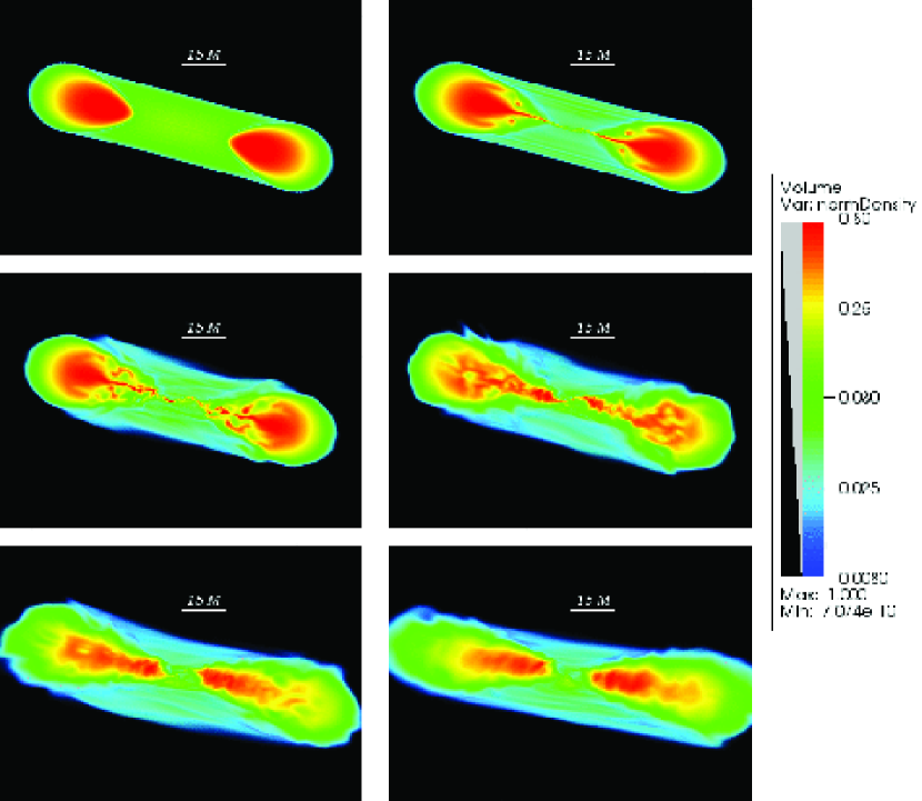
Figure 2: Volume visualization of the logarithm of density (scaled from $0.008\rho_{\rm max,0}$ to $0.8\rho_{\rm max,0}$) at (a) $t=0$, (b) 1, (c) 2, (d) 4, (e) 7, and (f) $10t_{\rm orb}$. Half of the disk has been cut away to reveal the cross section. The black hole spin axis is oriented vertically in each frame so that the initial torus is tilted $15^{\circ}$ to the right.

From orbits 1-2, MRI driven turbulence begins to grow in the inner parts of the disk. At the same time, some bending of the disk due to the differential precession from the hole becomes apparent. The MRI is fully developed through most of the disk around orbit 2.

By about orbit 7-8, the disk has reached a quasi-steady state. In the remainder of this section we detail the properties of the resultant structure. We follow an “inside-out” track, starting from key features of the flow near the hole and working toward larger radii. Where practical, we draw attention to similarities and differences between the quasi-steady structure that results in this simulation and the untilted simulations of De Villiers et al. (2003). In particular, we draw attention to the fact that some features, such as the inner torus and plunging region, are significantly altered, while others, such as the main body and coronal envelope, show very similar properties. Again, because of the varying levels of refinement along the poles, we do not discuss the evacuated funnel or funnel-wall jet in this paper.

3.1 Global Structure

3.1.1 Plunging Streams

Perhaps the most striking feature in the tilted disk at late times are the two opposing streams that start from high latitudes both with respect to the black-hole symmetry plane and the disk midplane (Fragile et al., 2007). Figure 3 shows a zoomed-in view of the region around the black hole including these streams. Note that stream 1 remains entirely above the black-hole symmetry plane, while stream 2 remains below. Clearly the material in each stream is in a plunging orbit into the black hole. Hence, we refer to these features as the “plunging streams.”

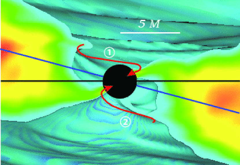
Figure 3: Zoomed in view of the inner $10r_{G}$ of the accretion flow revealing two opposing, high-latitude streams of material connecting the disk to the horizon (indicated by arrows). Data is taken from the last frame of the simulation ($t=10t_{\rm orb}$). To emphasize the plunging streams, the scaling in this figure is adjusted from that used in Fig. 2 by adding a density isosurface at $\rho=0.024\rho_{\rm max,0}$. The figure is oriented as in Fig. 2 with the black-hole spin axis vertical. The black-hole symmetry plane (black line) and initial disk midplane (blue line) are marked for reference. Note that stream 1 remains entirely above both planes while stream 2 remains below.

Figure 4 captures the plunging streams from a different perspective. This image is a view looking down the angular momentum axis of the black hole onto a single isodensity surface. The two opposing streams are clearly visible in the interior region of the disk as well as two relatively evacuated lobes.

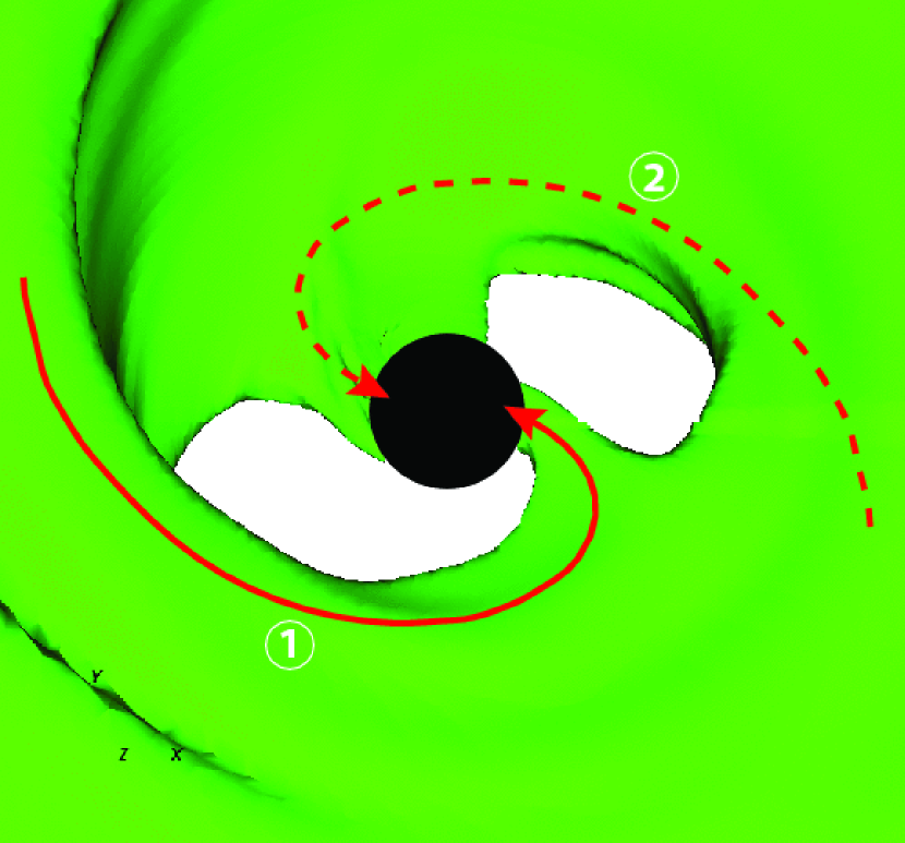
Figure 4: Isodensity contour at $\rho=0.1\rho_{\rm max,0}$ from the same time slice as Fig. 3 ($t=10t_{\rm orb}$) viewed down the angular momentum axis of the black hole. The initial disk angular momentum axis (and polar axis of the grid) is tilted $15^{\circ}$ to the right in this image. One plunging stream (indicated by solid arrow) starts near the left edge of the figure and connects to the hole on the right. This stream lies entirely above the black-hole symmetry plane and corresponds to stream 1 in Fig. 3. The opposing stream (stream 2) remains below the black-hole symmetry plane and is seen connecting with the horizon on the left.

As material passes through the plunging streams it undergoes strong differential precession. As we show below, the precession totals approximately $180^{\circ}$, accounting for how the material in the plunging streams is able to enter the black hole from the opposite azimuth from which it began its plunge without ever passing through the symmetry plane of the hole.

Two very important points to make about these streams is that they appear to be stable and stationary. They begin forming as early as $t=7t_{\rm orb}$ and last until the end of the simulation. During this time their azimuthal location does not change appreciably. The interesting questions are why do these opposing plunging streams form and why do they start from such high latitude with respect to the black-hole symmetry plane and disk midplane? The answers, of course, are related and the fundamental cause is the aspherical nature of the gravitational spacetime around the rotating black hole. This is best illustrated by considering the dependence of $r_{\rm ISCO}$ on inclination for orbits that are circular in the sense that they have constant coordinate radius. Briefly, $r_{\rm ISCO}$ is the radius at which the quantity

$$R\equiv A^{2}\left(\frac{\mathrm{d}r}{\mathrm{d}\tau}\right)^{2}=\left[E(r^{2}+a^{2})-aL_{z}\right]^{2}-\Delta\left[r^{2}+(L_{z}-aE)^{2}+Q\right]$$ (22)

and its first two derivatives equal zero, i.e. $R=R^{\prime}=R^{\prime\prime}=0$, where $E$, $L_{z}$, and $Q$ are the energy, angular momentum, and Carter constant, respectively, describing orbits around Kerr black holes (Hughes, 2001) and $A=r^{2}+a^{2}\cos^{2}\theta$ and $\Delta=r^{2}-2Mr+a^{2}$. Following Hughes (2001), we can eliminate $Q$ in favor of the inclination $i$ defined as

$$\cos i=\frac{L_{z}}{(L_{z}+Q)^{1/2}}~{}.$$ (23)

Figure 5 illustrates this dependence for a few selected cases of $a$. The key point of the formula and the plot is that orbital stability around a rotating black hole is strongly dependent on the inclination of the orbit. Notice that the unstable region increases monotonically for increasing inclination.

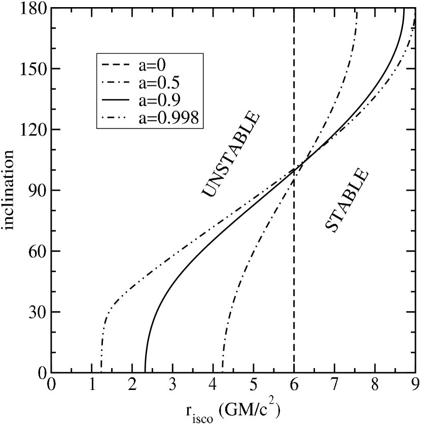
Figure 5: Plot of the inclination dependence of $r_{ISCO}$ for black-hole spins $a=0$, 0.5, 0.9, and 0.998. Inclinations $0\leq i\leq 90^{\circ}$ represent prograde orbits, whereas inclinations $90^{\circ}\leq i\leq 180^{\circ}$ represent retrograde orbits.

We can make better use of the information in Figure 5 by converting it to a polar plot (using only the prograde orbits) and overlaying it onto a plot of data from the simulation, as is done in Figure 6. Such a polar plot creates a representation of the prograde “ISCO surface” (symmetric about the spin axis of the black hole), which gives a clear indication of where the most unstable regions of the spacetime are. Note that the plunging orbits highlighted previously start near where the disk first encounters the ISCO surface. More precisely, the streams start near the largest cylindrical radius ($r\cos\vartheta$) of the ISCO surface, measured with respect to the angular momentum axis of the disk. This explains why the plunging streams start at such high inclinations relative to the black-hole symmetry plane and the disk midplane and why there are only two streams. The plunging region is no longer azimuthally symmetric from the perspective of the disk.

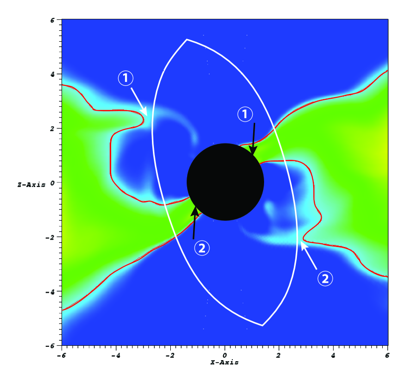
Figure 6: Meridional plot ($\varphi=0$) through the final dump ($t=10t_{\rm orb}$) of the simulation showing a pseudocolor representation of the logarithm of density (scaled from $0.008\rho_{\rm max,0}$ to $0.8\rho_{\rm max,0}$ as in previous figures) and an isocontour of density at $\rho=0.024\rho_{\rm max,0}$ (red curve). Unlike previous figures, this one is shown oriented in the sense of the grid, so that the black hole is tilted $15^{\circ}$ to the left. The plot is overlaid with a polar plot of the “ISCO surface” for prograde orbits about an $a=0.9$ black hole (white curve). This surface is symmetric about the spin axis of the hole. Notice that the plunging streams from Figs. 3 and 4 start near the largest cylindrical radius ($r\cos\vartheta$) of this surface (indicated by white arrows) and connect with the horizon approximately $180^{\circ}$ away in azimuth (indicated by black arrows).

Another point to take away from Figures 5 and 6 is that $r_{\rm ISCO}$ is larger for larger inclinations. Thus, for a given black-hole spin, plunging orbits will always start further away from the hole for more tilted disks. The tilted black hole effectively acts like an untilted black hole of lower spin, which would likewise have a larger $r_{\rm ISCO}$.

3.1.2 Inner Torus

In our tilted simulation, the plunging streams appear to connect directly to the main disk body without a clearly identifiable intermediate “inner torus”. This appears to be a particular result of the tilted simulation and not, for instance, due to the differences in the coordinates used in our simulation (Kerr-Schild) versus those used in De Villiers et al. (2003) (Boyer-Lindquist) or numerical techniques. We base this statement on the fact that our own untilted simulation in Kerr-Schild coordinates shows an inner torus very similar to the one described in De Villiers et al. (2003). For instance, Figure 7 shows the shell-averaged density and pressure as a function of radius for our tilted and untilted simulations. Shell averaged quantities are computed over the most refined grid as follows:

$$\langle\mathcal{Q}\rangle_{A}(r,t)=\frac{1}{A}\int^{2\pi}_{0}\int^{\vartheta_{2}}_{\vartheta_{1}}\mathcal{Q}\sqrt{-g}\mathrm{d}\vartheta\mathrm{d}\varphi~{},$$ (24)

where $A=\int^{2\pi}_{0}\int^{\vartheta_{2}}_{\vartheta_{1}}\sqrt{-g}\mathrm{d}\vartheta\mathrm{d}\varphi$ is the surface area of the shell. The data in Figure 7 has also been time-averaged over the final orbit, $9t_{\rm orb}=t_{\rm min}\leq t\leq t_{\rm max}=10t_{\rm orb}$, where time averages are defined as

$$\langle\mathcal{Q}\rangle_{t}=\frac{1}{t_{\rm max}-t_{\rm min}}\int^{t_{\rm max}}_{t_{\rm min}}\mathcal{Q}\mathrm{d}t~{}.$$ (25)

In the untilted simulation, both the density and the pressure show local maxima near $4.5r_{G}$, indicating an inner torus. The tilted simulation, on the other hand, shows only marginal evidence for local maxima near $10r_{G}$.

Figure 7: Plot of $\langle\langle\rho\rangle_{A}\rangle_{t}$ (solid line) and $\langle\langle P\rangle_{A}\rangle_{t}$ (dashed line) as a function of radius for equivalent (a) tilted $\beta_{0}=15^{\circ}$ (915h) and (b) untilted $\beta_{0}=0^{\circ}$ (90h) simulations. For both simulations, the data has been time-averaged over the interval $t=9$ to $10t_{\rm orb}$. The density and pressure have been normalized by their respective maxima at $t=0$, which are the same in both simulations.

Another check of the presence of an inner torus is to look at the distribution of specific angular momentum in the disk. Because the inner torus is partially supported by pressure gradients, some portion of the flow must be locally super-geodesic. In Figure 8 we plot the density-weighted shell average of the specific angular momentum $\langle\ell\rangle_{A}=\langle\rho\ell\rangle_{A}/\langle\rho\rangle_{A}$ as a function of radius, again time-averaged over the interval $t=9$ to $10t_{\rm orb}$. We compare this against the specific angular momentum distribution of circular orbits with inclinations of $15^{\circ}$ and $0^{\circ}$. These are calculated from the following expression

$$\ell=\frac{N_{1}+\Delta(Mr)^{1/2}N_{2}^{1/2}\cos i}{D}~{},$$ (26)

where

$$N_{1}=-aMr\left(3r^{2}+a^{2}-4Mr\right)\cos^{2}i~{},$$ (27)

$$N_{2}=r^{4}+a^{2}\sin^{2}i\left(a^{2}+2r^{2}-4Mr\right)~{},$$ (28)

and

$$D=a^{2}\left(2r^{2}+a^{2}-3Mr\right)\sin^{2}i+r^{4}+4M^{2}r^{2}-4r^{3}M-Mra^{2}~{},$$ (29)

which comes from noting that for circular orbits $R=R^{\prime}=0$ from equation (22) and from the definition $\ell=L_{z}/E$. Both simulations show a nearly geodesic angular momentum distribution through most of the disk with a small region of super-geodesic flow inside $10r_{G}$. This region clearly corresponds to the inner torus in the untilted simulation. It also suggests that there should be an inner torus in the tilted simulation, though, again, this is not as evident in the plots of density and pressure.

Figure 8: Plot of the density-weighted time- and shell-averaged specific angular momentum $\langle\langle\ell\rangle_{A}\rangle_{t}$ (thick line) as a function of radius for equivalent (a) tilted $\beta_{0}=15^{\circ}$ (915h) and (b) untilted $\beta_{0}=0^{\circ}$ (90h) simulations. For both simulations, the data has been time-averaged over the interval $t=9$ to $10t_{\rm orb}$. In each plot a comparison is provided with the specific angular momentum of circular orbits with inclinations of $15^{\circ}$ and $0^{\circ}$, respectively (dashed line). For reference we also include the initial angular momentum distribution in the midplane of the torus (thin line).

Another indication that the inner torus is less prominent in the tilted simulation than the untilted one comes from comparing the total rest mass in the near-hole region ($r<r_{\rm cut}=10r_{G}$). This is done in Figure 9, where we plot the time histories of the total (volume-integrated) rest mass

$$\left\langle\rho u^{0}\right\rangle_{V}=\int^{2\pi}_{0}\int^{\pi}_{0}\int^{r_{\rm cut}}_{r_{\rm min}}D\mathrm{d}r\mathrm{d}\vartheta\mathrm{d}\varphi~{}.$$ (30)

At $t=10t_{\rm orb}$, the inner torus is 42% less massive in Model 915h.

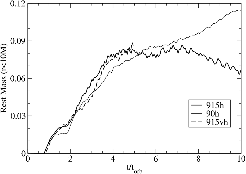
Figure 9: Total rest mass in the near-hole region ($r<10r_{G}$) as a function of time for the tilted (915h & 915vh) and untilted (90h) simulations. The mass and time are normalized by the initial mass and orbital period of the torus, respectively.

When present, the inner torus usually performs two functions: regulating the accretion of matter into the black hole and serving as the launching point for the funnel-wall jet. Therefore, we may expect a weaker funnel-wall jet (to be discussed in future work) and a higher mass accretion rate in our tilted-disk simulation relative to the untilted simulation due to the less prominent inner torus in the former. We compute the mass accretion rate

$$\dot{M}(r)=\int^{2\pi}_{0}\int^{\pi}_{0}DV^{r}\mathrm{d}\vartheta\mathrm{d}\varphi$$ (31)

100 times per $t_{\rm orb}$ (about every $8M$) at each of the external grid boundaries. Figure 10a shows a plot comparing $\dot{M}(r_{\rm min})$ for our equivalent tilted and untilted simulations. When averaged over the quasi-steady state of each simulation (from $t=7$ to $10t_{\rm orb}$), $\langle\dot{M}\rangle_{t}$ into the hole for the tilted simulation (915h) is $7.2\times 10^{-6}$, while for the untilted one (90h), it is $4.9\times 10^{-6}$. There is a clear tendancy toward a higher $\dot{M}$ in the tilted-disk simulation.

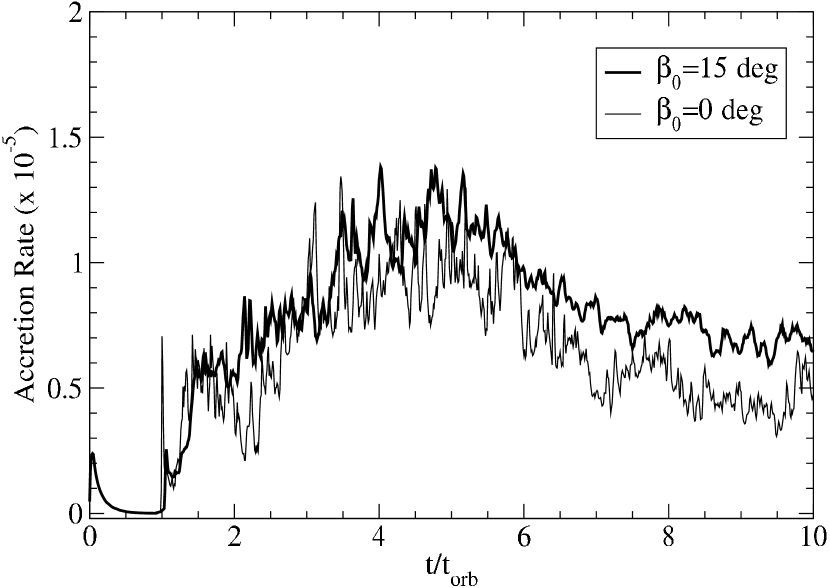
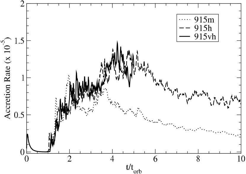
Figure 10: (a) Plot of the mass accretion history from Model 915h with $\beta_{0}=15^{\circ}$ (thick line) and Model 90h with $\beta_{0}=0^{\circ}$ (thin line). The accretion rate and time are normalized by the initial mass and orbital period of the torus, respectively. (b) Plot of mass accretion rate, comparing our medium (915m), high (915h), and very high (915vh) resolution tilted disk simulations. The very high resolution simulation was only run to $t=5t_{\rm orb}$.

Figure 10b compares $\dot{M}$ of the tilted disk simulation at three different resolutions. Due to the chaotic nature of the mass accretion we do not expect the individual peaks to match; yet we are encouraged that the overall shape and magnitude of the two high-resolution models (915h and 915vh) are very consistent, suggesting we are reasonably well converged. The medium resolution simulation (Model 915m), on the other hand, is clearly underresolved.

3.1.3 Main Disk Body & Coronal Envelope

The main disk body does not differ substantially between the tilted and untilted simulations, except in the notable fact that the tilted disk precesses (as discussed in §3.2.2 below). Likewise, the coronal envelope, which extends above and below the disk, shows very similar properties in all our simulations. The material in the coronal envelope is characterized by low density and rough magnetic equipartition ($\beta_{\rm mag}\approx 1$). By contrast the main body of the disk is generally gas-pressure dominated ($\beta_{\rm mag}\ll 1$). Therefore, a plot of $\beta_{\rm mag}$ and $\rho$, such as Figure 11, provides a convenient means to identify these two regions. As found in De Villiers et al. (2003), the material in the coronal envelope moves mostly radially outward, yet has ($-hu_{t}<1$). This suggests that the material may be gravitationally bound, in which case it must circulate back to the disk at large radii. However, we point out that this definition of binding energy ignores the contribution of the magnetic fields, so some of this material may in fact escape the system. We plan to examine outflows from tilted disks more thoroughly in future work.

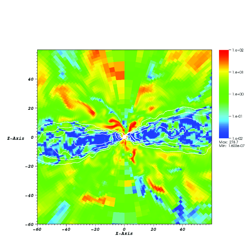
Figure 11: Azimuthal slice through the simulation along $\varphi=0$ taken from the final dump ($t=10t_{\rm orb}$). The ratio of magnetic pressure to gas pressure ($\beta_{\rm mag}^{-1}$) is represented as a pseudocolor plot. The colors are scaled logarithmically and cover the range $10^{-2}\leq\beta_{\rm mag}\leq 10^{2}$. The gas density is given by isocontours at $\rho=10^{-2}$, $10^{-1.5}$, $10^{-1}$, and $10^{-0.5}\rho_{\rm max,0}$. As with Fig. 6, this figure is oriented in the sense of the grid, so that the black hole is tilted $15^{\circ}$ to the left. The apparent tilt of the disk is actually due its precession about the black-hole spin axis, such that the angular momentum axis of the disk is no longer in the plane of this image; the disk has not actually realigned with the hole. We remind the reader that the region near the poles is not sufficiently resolved, so caution should be used when interpreting results there.

Because the disk is precessing, its angular momentum axis does not remain aligned with the grid. Therefore, an azimuthal slice through the disk at late times, such as Figure 11, may give the impression that the disk has aligned with the symmetry plane of the black hole when indeed this is not the case. We now turn to the question of disk alignment and precession.

3.2 Results Specific to A Tilted Disk

3.2.1 Tilt

One key diagnostic for describing the global response of a tilted disk subject to Lense-Thirring precession is the tilt between the angular momenta of the black hole and disk as a function of radius and time. For example, in the Bardeen-Petterson solution, no time variability is observed, and the tilt transitions from nearly zero close to the black hole to a non-zero asymptote at large radii.

As in Fragile & Anninos (2005), we recover the tilt from the simulation data using the definition

$$\beta(r)=\arccos\left[\frac{\mathbf{J}_{\rm BH}\cdot\mathbf{J}_{\rm Disk}(r)}{|\mathbf{J}_{\rm BH}||\mathbf{J}_{\rm Disk}(r)|}\right]~{},$$ (32)

where

$$\mathbf{J}_{\rm BH}=\left(-aM\sin\beta_{0}\hat{x},0,aM\cos\beta_{0}\hat{z}\right)$$ (33)

is the angular momentum vector of the black hole and

$$\mathbf{J}_{\rm Disk}(r)=\left[(J_{\rm Disk})_{1}\hat{x},(J_{\rm Disk})_{2}\hat{y},(J_{\rm Disk})_{3}\hat{z}\right]$$ (34)

is the angular momentum vector of the disk in an asymptotically flat space. This is given by

$$(J_{\rm Disk})_{\rho}=\frac{\epsilon_{\mu\nu\sigma\rho}L^{\mu\nu}S^{\sigma}}{2\sqrt{-S^{\alpha}S_{\alpha}}}~{},$$ (35)

where

$$L^{\mu\nu}=\int\left(x^{\mu}T^{\nu 0}-x^{\nu}T^{\mu 0}\right)\mathrm{d}^{3}x,$$ (36)

and $S^{\sigma}=\int T^{\sigma 0}\mathrm{d}^{3}x$. The equations for $L^{\mu\nu}$ and $S^{\sigma}$ are integrated over concentric radial shells of the most-refined grid layer, e.g.

$$S^{\sigma}(r)=\int^{2\pi}_{0}\int^{\vartheta_{2}}_{\vartheta_{1}}T^{\sigma 0}\sqrt{-g}\Delta r\mathrm{d}\vartheta\mathrm{d}\varphi~{}.$$ (37)

The unit vector $\hat{y}$ points along the axis about which the black hole is initially tilted and $\hat{z}$ points along the initial angular momentum axis of the disk.

In Figure 12, we show the radial profile of $\beta$ time averaged over the interval $9t_{\rm orb}\leq t\leq 10t_{\rm orb}$. Recall $\beta_{0}=15^{\circ}$ for this simulation. This profile remains fairly consistent over many orbital times once the quasi-steady state is reached, so the time-averaged data gives a good representation for all $t\gtrsim 7t_{\rm orb}$. The variability from this time-averaged profile is generally $\lesssim 20\%$ and is generally carried by moderate amplitude waves traveling through the disk. The increase in tilt at $r\lesssim 10r_{G}$ is attributable to the high latitude plunging streams described in §3.1.1.

Figure 12: Plot of the tilt $\langle{\beta}\rangle_{t}$ as a function of radius through the disk. The data for this plot has been time averaged from $t=9$ to $10t_{\rm orb}$. The initial tilt was $\beta_{0}=15^{\circ}$.

One very obvious characteristic of the profile in Figure 12 is that $\beta$ does not approach zero except perhaps very close to the hole. Thus we do not see evidence for the Bardeen-Petterson effect in this simulation. This is not surprising since the Bardeen-Petterson solution is only expected for thin disks ($H/r<\alpha$). This is not the applicable regime for this simulation, as we illustrate in Figure 13, which shows $H/r$ and $\alpha$ plotted as functions of $r$. The scale height $H(r)$ is defined in each radial shell as one-half the distance ($0.5r\Delta\vartheta$) between the two points where $\rho=\rho_{max}/e$, where we use the time-averaged density along the $\varphi=0$ azimuthal slice. The dimensionless stress parameter $\alpha$ in the disk is taken to be

$$\alpha=\left\langle\frac{|u^{r}u^{\varphi}||B||^{2}-B^{r}B^{\varphi}|}{4\pi P}\right\rangle_{A}~{}.$$ (38)

We restrict the calculation of $\alpha$ to only bound material ($-hu_{t}<1$). Using these definitions we find $H/r\sim 0.2$ and $\alpha\lesssim 0.01$ through most of the disk.

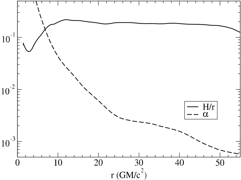
Figure 13: Plot of the scale height $\langle H\rangle_{t}/r$ and magnetic stress parameter $\langle\alpha\rangle_{t}$, time averaged over the interval $7t_{\rm orb}\leq t\leq 10t_{\rm orb}$. This plot shows that this simulation falls into the thick-disk limit $H/r>\alpha$.

Since warps in slim disks are expected to propagate as bending waves, it may seem unusual at first that we see little evidence for such waves in Figure 12. For instance, Lubow et al. (2002) provides an analysis of the theory of bending waves in nearly Keplerian, weakly inclined disks and predicts that the tilt $\beta$ should be a time-independent, oscillatory function of radius (see also Marković & Lamb, 1998). However, using equation (16) of Lubow et al. (2002), we estimate the wavelength of such oscillations for our simulation to be

$$\lambda\approx\frac{\pi r^{9/4}}{(6a)^{1/2}}\left(\frac{H}{r}\right)\sim 50M$$ (39)

at $r=10r_{G}$. This is strongly radially dependent ($\lambda\propto r^{9/4}$ with $H/r\sim\mathrm{constant}$), so oscillations of $\beta$ are essentially absent outside $r=10r_{G}$, consistent with what is shown in Figure 12.

The same conclusion, that $\beta$ is not expected to oscillate outside $r=10r_{G}$ for this simulation, is also reached by considering equation (22) of Lubow et al. (2002). That equation defines a dimensionless variable

$$x=\left(\frac{24a}{\epsilon^{2}}\right)^{1/2}\frac{r^{-(h+1/4)}}{h+1/4}~{},$$ (40)

which is used to identify the transition radius between oscillatory behavior and asymptotic behavior, where $h$ and $\epsilon$ are used to parameterize the radial dependence of the disk scale height $H/r=\epsilon r^{h-1}$. Whenever $x>>1$ (small $r$), oscillations should be prominent, whereas whenever $x<<1$ (large $r$), $\beta$ tends to the outer boundary value. For our simulation, with $\epsilon\approx 0.2$ and $h\approx 1$, $x=1$ at $r\approx 10r_{G}$. Thus, from both approaches, it is clear that our simulation does not satisfy the criteria to develop large oscillations in $\beta$ within the main body of the disk.

Inside $r=10r_{G}$, the density of the disk drops off rapidly and the dynamics are dominated by the plunging streams, which are not accounted for in the model of Lubow et al. (2002). Nevertheless, we appear to capture one-half of one wavelength of a bending wave oscillation inside $r=10r_{G}$, based on Figure 12. Thus, overall our results seem to be generally consistent with the predictions of Lubow et al. (2002).

3.2.2 Precession

A second useful diagnostic for tilted disks is the twist $\gamma$ of the disk as a function of radius and time. We define the precession angle (twist) as

$$\gamma(r)=\arccos\left[\frac{\mathbf{J}_{\rm BH}\times\mathbf{J}_{\rm Disk}(r)}{|\mathbf{J}_{\rm BH}\times\mathbf{J}_{\rm Disk}(r)|}\cdot\hat{y}\right]~{},$$ (41)

From this definition, $\gamma(r)=0$ throughout the disk at $t=0$. In order to capture twists larger than $180^{\circ}$, we also track the projection of $\mathbf{J}_{\rm BH}\times\mathbf{J}_{\rm Disk}(r)$ onto $\hat{x}$, allowing us to break the degeneracy in $\arccos$. A time-averaged plot of $\gamma$ is provided in Figure 14.

Figure 14: Plot of the twist $\langle\gamma\rangle_{t}$ as a function of radius through the disk. The data for this plot has been time averaged from $t=9$ to $10t_{\rm orb}$. Initially the twist was zero throughout the disk. The disk matter has precessed roughly $\sim 180^{\circ}$ by the time it reaches the hole. The shape of this twist profile remains fairly constant throughout the simulation.

As described in our previous work (Fragile & Anninos, 2005), we expect differential Lense-Thirring precession to dominate whenever the precession timescale $t_{\rm LT}=\Omega_{\rm LT}^{-1}=g^{tt}/g^{t\phi}$ is shorter than local dynamical timescales in the disk (Bardeen & Petterson, 1975; Kumar & Pringle, 1985). We consider three possible limiting timescales: the mass accretion timescale $t_{\rm acc}=r/\overline{V}^{r}$, where $\overline{V}^{r}=\langle\langle\rho V^{r}\rangle_{A}/\langle\rho\rangle_{A}\rangle_{t}$ is the density-weighted average inflow velocity; the sound-crossing time $t_{cs}=r/\overline{c}_{s}$, where $\overline{c}_{s}=\langle\langle\rho c_{s}\rangle_{A}/\langle\rho\rangle_{A}\rangle_{t}$ is a density-weighted average of the local sound speed; and the Alfvén crossing time $t_{A}=r/\overline{V}_{A}$, where $\overline{V}_{A}$ is a density-weighted average of the local Alfvén speed. The local sound speed is recovered from the fluid state through the relation $c_{s}^{2}=\Gamma(\Gamma-1)P/[(\Gamma-1)\rho+\Gamma P]$. The Alfvén speed is

$$v_{A}=\sqrt{\frac{||B||^{2}}{4\pi\rho h+||B||^{2}}}~{}.$$ (42)

Since $c_{s}$ and $v_{A}$ are defined in the frame of the fluid, it is not strictly accurate to compare $t_{cs}$ and $t_{A}$ to quantities defined using the coordinate time (such as $t_{\rm LT}$ and $\Omega^{-1}$). However, we are mostly concerned with the timescales in the main body of the disk where such discrepancies are small. From Figure 15, we can see that the Lense-Thirring precession timescale is longer than the sound-crossing time at virtually all radii.

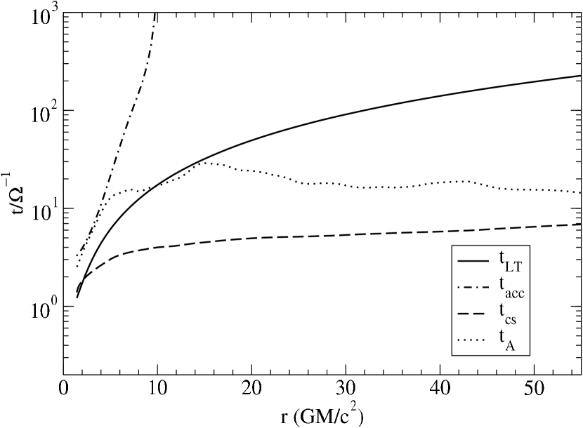
Figure 15: Plot comparing various timescales within the disk, including the Lense-Thirring precession timescale $t_{\rm LT}$, the accretion timescale $t_{\rm acc}$, the sound-crossing time $t_{\rm cs}$, and the Alfvén crossing time $t_{\rm A}$. All timescales are normalized by the local orbital period in the midplane of the black hole, $\Omega^{-1}$. The data for this plot has been time averaged from $t=9t_{\rm orb}$ to $t=10t_{\rm orb}$.

Since the sound-crossing time is short compared to the precession timescale throughout the bulk of the disk, pressure waves strongly couple the disk material. The disk, thus, responds as a single entity to the torque of the black-hole and precesses as a global structure. Such global precession has been noted before in low Mach number hydrodynamic disks (Nelson & Papaloizou, 2000; Fragile & Anninos, 2005). To estimate the precession period, we have plotted $\gamma$, averaged over the bulk of the disk ($20\leq r/r_{G}\leq 50$), as a function of time in Figure 16. A linear fit to this plot yields a precession period of $T_{\rm prec}\approx 0.3(M/M_{\odot})$ s, which corresponds to about $80t_{\rm orb}$. This is longer than the evolution time of all of our models, so we have had to extrapolate the full precession period. However, Model 915m is run to $20t_{\rm orb}$ and shows a nearly linear growth of precession over the full simulation.

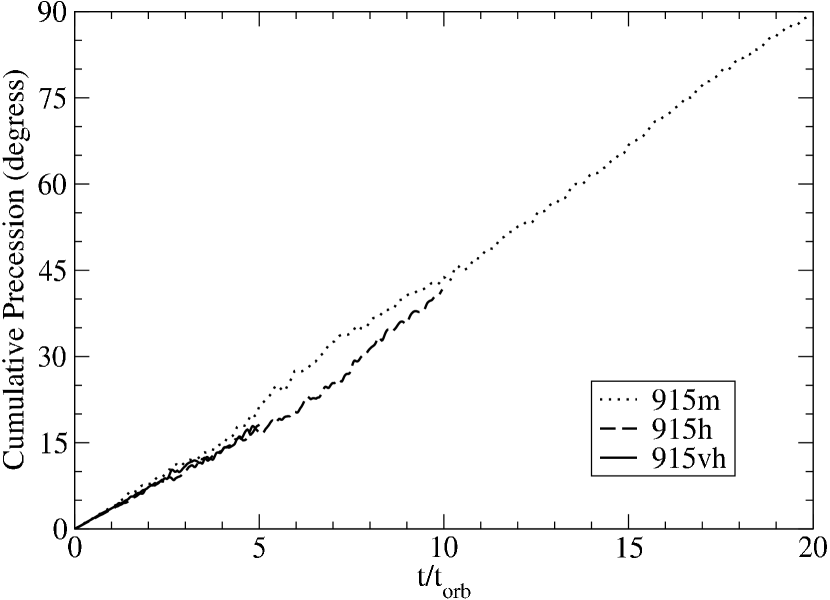
Figure 16: Plot of the twist $\gamma$, averaged over the bulk of the disk ($20\leq r/r_{G}\leq 50$), as a function of time. The slope of this plot can be used to estimate the precession period of the disk as a whole, which is $0.3(M/M_{\odot})$ s.

Classically, we expect the precession period for a solid-body rotator with angular momentum $J$ subject to a torque $\tau$ to be $T_{\rm prec}=2\pi(\sin\beta)(J/\tau)$ (Liu & Melia, 2002). Assuming a radial dependence to the surface density of the form $\Sigma=\Sigma_{i}(r/r_{i})^{-\zeta}$ and ignoring higher order general relativistic corrections, we have $J=2\pi M^{1/2}\Sigma_{i}r_{i}^{\zeta}r_{0}^{5/2-\zeta}[1-(r_{i}/r_{o})^{5/2-\zeta}]/(5/2-\zeta)$ and $\tau=4\pi(\sin\beta)aM^{3/2}\Sigma_{i}[1-(r_{i}/r_{o})^{1/2+\zeta}]/[r_{i}^{1/2}(1/2+\zeta)]$, where $r_{i}$ and $r_{o}$ are the inner and outer radii of the evolved disk, respectively. Therefore,

$$T_{\rm prec}=\frac{\pi(1+2\zeta)}{(5-2\zeta)}\frac{r_{o}^{5/2-\zeta}r_{i}^{1/2+\zeta}\left[1-(r_{i}/r_{o})^{5/2-\zeta}\right]}{aM\left[1-(r_{i}/r_{o})^{1/2+\zeta}\right]}~{}.$$ (43)

For $r_{i}=10r_{G}$, $r_{o}=50r_{G}$, and $\zeta=0$ (the value we find in our simulation), equation (43) predicts $T_{\rm prec}=0.3(M/M_{\odot})$ s, which is the same as the observed value in the simulation. Note that equation (43) differs from the test particle Lense-Thirring precession period because $T_{\rm prec}$ depends on the total torque integrated over the entire disk.

4 Discussion

In this paper we studied the evolution of an MRI turbulent disk that was tilted with respect to the spin axis of a modestly fast rotating black hole. Although this prescription can lead to a Bardeen-Petterson configuration for some disk parameters, we did not see evidence for this in this simulation, as alignment of the disk with the equatorial plane of the black hole did not occur. This is not surprising since this simulation was carried out in the thick-disk regime where $H/r>\alpha$ and warps produced in the disk propagate as waves (Papaloizou & Lin, 1995), rather than diffusively as in the Bardeen-Petterson case. Since the expected bending wavelength (Lubow et al., 2002) turned out to be longer than the radial extent of the disk in the simulation, little warping of the disk was observed. Instead the unwarped disk precessed uniformly. The extrapolated precession period $T_{\rm prec}\approx 0.3(M/M_{\odot})$ s equates to periods of $\approx 3$ s and $\approx 3$ d for black holes of mass $M=10M_{\odot}$ and $M=10^{6}M_{\odot}$, respectively. Such global disk precession could explain certain variability features observed from accreting black holes, such as low-frequency QPOs (LFQPOs) (Stella et al., 1999; Liu & Melia, 2002; Schnittman et al., 2006), since the observer’s viewing angle of the inner, X-ray emitting region of the disk would vary periodically.

If the inner disk is optically thick enough to produce relativistically-broadened reflection features, such as an iron K$\alpha$ line, then such precession should also be observable through periodic changes in both the shape and strength of the lines (Fragile et al., 2005). These changes should be correlated with the phase of the corresponding LFQPO. Such a correlation has been observed in GRS 1915+105 (Miller & Homan, 2005), although only between line strength and QPO phase; those data were not sufficiently resolved to determine the line shape.

Generally, we expect the precession period to be given by equation (43), which has a strong dependence on the radial distribution of the disk ($\propto r_{o}^{5/2-\zeta}r_{i}^{1/2+\zeta}$). One idea to consider is that the outer radius may correspond to the truncation radius proposed to explain the hard state of black hole X-ray binaries (e.g. Esin et al. (1997), but see also Rykoff et al. (2007)). In this case our simulated disk would represent the hot, geometrically thick flow that fills the region inside the truncation radius. The LFQPO would then correspond to the precession frequency of this inner flow, in which case it should scale as $r_{o}^{-5/2+\zeta}$. Sobczak et al. (2000) explored the dependence of the LFQPO frequency on spectral fitting parameters, including what would be the truncation radius in the context of the suggested hard state model. They studied two sources, XTE J1550-564 and GRO J1655-40, and found opposite trends between frequency and radius. For XTE J1550-564 the observed frequency was $\nu_{\rm LFQPO}\sim 5$ Hz, and the observed truncation radius was $r_{o}/r_{G}=2.7(10M_{\odot}/M)(D/6\rm{~{}kpc})(\cos\theta)^{-1/2}$. From equation (43) we would expect

$$\frac{r_{o}}{r_{G}}=\left[\frac{5-2\zeta}{\pi(1+2\zeta)}\right]^{2/(5-\zeta)}\left(\frac{a}{M}\right)^{2/(5-\zeta)}\left(\frac{r_{i}}{r_{G}}\right)^{-(1+2\zeta)/(5-2\zeta)}\left(\nu M\right)^{-2/(5-\zeta)}~{}.$$ (44)

In our simulation we found $\zeta\approx 0$, which gives $r_{o}\approx 33r_{G}$ for $M=10M_{\odot}$ and $\nu=5$ Hz. This is considerably larger than the observed value. However, some of the discrepancy may be attributable to the large uncertainties in the parameters used to describe this source, including its distance, mass, and inclination. Also, if the surface density in XTE J1550-564 depends strongly on radius, which was not the case for our simulated disk, then our prediction would change significantly. Further observational studies along this line are needed to test this prediction more thoroughly.

Although the main body of the disk was not significantly altered by the tilt, we did find significant differences in the inner regions of the flow when compared with untilted simulations. First, a tilted disk encounters the generalized ISCO surface at a larger radius than an untilted disk. This causes the plunging region to start further out. The binding energy of the innermost material in the disk is therefore less than it would be for an aligned disk, and the overall radiative efficiency should then be reduced.

On the other hand, tilting the disk appears to produce a higher overall mass accretion rate (shown here in Figure 10a; also discussed in Lodato & Pringle, 2006). A tilted accretion disk will therefore have a lower surface density than an untilted disk with the same accretion rate. This may affect the emergent spectrum, especially for hot, optically thin flows. On the other hand for flows that are effectively optically thick, Davis et al. (2005) found that the emergent spectra are remarkably independent of the overall stress and surface density.

We also found that the plunging region is not axially symmetric. Instead, accretion onto the hole in the tilted-disk case occurs through two discrete streams of material that leave the disk at high latitudes with respect to the black-hole and disk symmetry planes. This may affect the magnitude of magnetic torques exerted by the plunging region on the disk. An interesting question for future work is how these streams vary on the timescale of the precession of the disk. We intend to explore the detailed properties of the plunging region and innermost disk in a future paper.

The tilted disk also seems not to have formed a clearly identifiable inner torus. This could be significant because the inner torus serves as a launching point for the matter-dominated, funnel-wall jet. The absence of a prominent inner torus may lead to a weaker matter jet. However, the present simulation is not suited to addressing this issue because of the poor and varying resolution used near the pole. Instead, we plan to explore jets and outflows from tilted disks in future work.

In many respects the tilted disk simulation exhibited properties consistent with an untilted disk around a black hole of lower spin. These included the larger plunging radius, higher mass accretion rate, and less prominent inner torus. Thus black-hole tilt could hamper efforts to estimate black-hole spin based on such properties. Indeed, it is commonly stated that astrophysical black hole spacetimes depend on just two parameters: mass and spin. But it should be remembered that the observed properties of black hole accretion disks also depend on their inclinations with respect to the spin axes of their central black holes. This inclination should be a target of future observational programs that use accretion disks as surrogates to study properties of black holes.

References

- Anninos & Fragile (2003) Anninos, P., & Fragile, P. C. 2003, ApJS, 144, 243
- Anninos et al. (2005) Anninos, P., Fragile, P. C., & Salmonson, J. D. 2005, ApJ, 635, 723
- Balbus & Hawley (1991) Balbus, S. A., & Hawley, J. F. 1991, ApJ, 376, 214
- Bardeen & Petterson (1975) Bardeen, J. M., & Petterson, J. A. 1975, ApJ, 195, L65
- Caproni et al. (2007) Caproni, A., Abraham, Z., Livio, M., & Mosquera Cuesta, H. J. 2007, MNRAS
- Caproni et al. (2006) Caproni, A., Abraham, Z., & Mosquera Cuesta, H. J. 2006, ApJ, 638, 120
- Chakrabarti (1985) Chakrabarti, S. K. 1985, ApJ, 288, 1
- Davis et al. (2005) Davis, S. W., Blaes, O. M., Hubeny, I., & Turner, N. J. 2005, ApJ, 621, 372
- Davis et al. (2006) Davis, S. W., Done, C., & Blaes, O. M. 2006, ApJ, 647, 525
- De Villiers & Hawley (2003a) De Villiers, J., & Hawley, J. F. 2003a, ApJ, 589, 458
- De Villiers & Hawley (2003b) De Villiers, J., & Hawley, J. F. 2003b, ApJ, 592, 1060
- De Villiers et al. (2003) De Villiers, J., Hawley, J. F., & Krolik, J. H. 2003, ApJ, 599, 1238
- Esin et al. (1997) Esin, A. A., McClintock, J. E., & Narayan, R. 1997, ApJ, 489, 865
- Font et al. (1998) Font, J. A., Ibáñez, J. M. ., & Papadopoulos, P. 1998, ApJ, 507, L67
- Fragile & Anninos (2005) Fragile, P. C., & Anninos, P. 2005, ApJ, 623, 347
- Fragile & Anninos (2007) Fragile, P. C., & Anninos, P. 2007, ApJ, 666, xxx
- Fragile et al. (2007) Fragile, P. C., Anninos, P., Blaes, O. M., & Salmonson, J. D. 2007, in proceedings of the 11th Marcel Grossmann Meeting on General Relativity (astro-ph/0701272)
- Fragile et al. (2001) Fragile, P. C., Mathews, G. J., & Wilson, J. R. 2001, ApJ, 553, 955
- Fragile et al. (2005) Fragile, P. C., Miller, W. A., & Vandernoot, E. 2005, ApJ, 635, 157
- Gammie et al. (2003) Gammie, C. F., McKinney, J. C., & Tóth, G. 2003, ApJ, 589, 444
- Hannikainen et al. (2001) Hannikainen, D., Campbell-Wilson, D., Hunstead, R., McIntyre, V., Lovell, J., Reynolds, J., Tzioumis, T., & Wu, K. 2001, Astrophysics and Space Science Supplement, 276, 45
- Hawley (1991) Hawley, J. F. 1991, ApJ, 381, 496
- Hawley (2000) Hawley, J. F. 2000, ApJ, 528, 462
- Hawley et al. (1984) Hawley, J. F., Smarr, L. L., & Wilson, J. R. 1984, ApJS, 55, 211
- Hughes (2001) Hughes, S. A. 2001, Phys. Rev. D, 64, 064004
- Koide et al. (1999) Koide, S., Shibata, K., & Kudoh, T. 1999, ApJ, 522, 727
- Komissarov (2006) Komissarov, S. S. 2006, MNRAS, 368, 993
- Kondratko et al. (2005) Kondratko, P. T., Greenhill, L. J., & Moran, J. M. 2005, ApJ, 618, 618
- Krolik (1999) Krolik, J. H. 1999, Active Galactic Nuclei : From the Central Black Hole to the Galactic Environment (Princeton, N. J. : Princeton University Press)
- Kumar & Pringle (1985) Kumar, S., & Pringle, J. E. 1985, MNRAS, 213, 435
- Liu & Melia (2002) Liu, S., & Melia, F. 2002, ApJ, 573, L23
- Lodato & Pringle (2006) Lodato, G., & Pringle, J. E. 2006, MNRAS, 368, 1196
- Lubow et al. (2002) Lubow, S. H., Ogilvie, G. I., & Pringle, J. E. 2002, MNRAS, 337, 706
- Maccarone (2002) Maccarone, T. J. 2002, MNRAS, 336, 1371
- Marković & Lamb (1998) Marković , D., & Lamb, F. K. 1998, ApJ, 507, 316
- McClintock & Remillard (2005) McClintock, J. E., & Remillard, R. A. 2005, in Compact Stellar X-ray Sources, in press (astro-ph/0306213)
- McKinney (2006) McKinney, J. C. 2006, MNRAS, 368, 1561
- Miller & Homan (2005) Miller, J. M., & Homan, J. 2005, ApJ, 618, L107
- Nelson & Papaloizou (2000) Nelson, R. P., & Papaloizou, J. C. B. 2000, MNRAS, 315, 570
- Orosz & Bailyn (1997) Orosz, J. A., & Bailyn, C. D. 1997, ApJ, 477, 876
- Orosz et al. (2002) Orosz, J. A., et al. 2002, ApJ, 568, 845
- Papadopoulos & Font (1998) Papadopoulos, P., & Font, J. A. 1998, Phys. Rev. D, 58, 24005
- Papaloizou & Lin (1995) Papaloizou, J. C. B., & Lin, D. N. C. 1995, ApJ, 438, 841
- Rykoff et al. (2007) Rykoff, E. S., Miller, J. M., Steeghs, D., & Torres, M. A. P. 2007, ArXiv Astrophysics e-prints
- Schnittman et al. (2006) Schnittman, J. D., Homan, J., & Miller, J. M. 2006, ApJ, 642, 420
- Shakura & Sunyaev (1973) Shakura, N. I., & Sunyaev, R. A. 1973, A&A, 24, 337
- Sobczak et al. (2000) Sobczak, G. J., McClintock, J. E., Remillard, R. A., Cui, W., Levine, A. M., Morgan, E. H., Orosz, J. A., & Bailyn, C. D. 2000, ApJ, 531, 537
- Stella et al. (1999) Stella, L., Vietri, M., & Morsink, S. M. 1999, ApJ, 524, L63
- Wilson (1972) Wilson, J. R. 1972, ApJ, 173, 431