A constrained scheme for Einstein equations based on Dirac gauge and spherical coordinates

Abstract

We propose a new formulation for 3+1 numerical relativity, based on a constrained scheme and a generalization of Dirac gauge to spherical coordinates. This is made possible thanks to the introduction of a flat 3-metric on the spatial hypersurfaces $t={\rm const}$, which corresponds to the asymptotic structure of the physical 3-metric induced by the spacetime metric. Thanks to the joint use of Dirac gauge, maximal slicing and spherical components of tensor fields, the ten Einstein equations are reduced to a system of five quasi-linear elliptic equations (including the Hamiltonian and momentum constraints) coupled to two quasi-linear scalar wave equations. The remaining three degrees of freedom are fixed by the Dirac gauge. Indeed this gauge allows a direct computation of the spherical components of the conformal metric from the two scalar potentials which obey the wave equations. We present some numerical evolution of 3-D gravitational wave spacetimes which demonstrates the stability of the proposed scheme.

I Introduction and motivations

Motivated by the construction of the detectors LIGO, GEO600, TAMA and VIRGO, as well as by the space project LISA, numerical studies of gravitational wave sources are numerous (see BaumgS03 ; Lehne01 for recent reviews). The majority of them are performed within the framework of the so-called 3+1 formalism of general relativity, also called Cauchy formulation, in which the spacetime is foliated by a family of spacelike hypersurfaces. We propose here a new strategy within this formalism, based on a constrained scheme and spherical coordinates, which is motivated as follows.

I.1 Motivations for a constrained scheme

In the 3+1 formalism, the Einstein equations are decomposed in a set of four constraint equations and a set of six dynamical equations York79 ; BaumgS03 . The constraint equations give rise to elliptic (or sometime parabolic) partial differential equations (PDE), whereas the PDE type of the dynamical equations depends on the choice of the coordinate system. Various strategies can then be contemplated: (i) free evolution scheme: solving the constraint equations only to get the initial data and performing the time evolution via the dynamical equations, without enforcing the constraints; (ii) partially constrained scheme: using some of the constraints to compute some of the metric components during the evolution and (iii) fully constrained scheme: solving the four constraint equations at each time step.

In the eighties, partially constrained schemes, with only the Hamiltonian constraint enforced, have been widely used in 2-D (axisymmetric) computations (e.g. Bardeen and Piran BardeP83 , Stark and Piran StarkP85 , Evans Evans86 ). Still in the 2-D axisymmetric case, fully constrained schemes have been used by Evans Evans89 and Shapiro and Teukolsky ShapiT92 for non-rotating spacetimes, and by Abrahams, Cook, Shapiro and Teukolsky AbrahCST94 for rotating ones. We also notice that the recent (2+1)+1 axisymmetric code of Choptuik et al. ChoptHLP03 is based on a constrained scheme too.

Regarding the 3-D case, almost all numerical studies to date are based on free evolution schemes. It turned out that the free evolution scheme directly applied to the standard 3+1 equations (sometimes called ADM formulation) failed due to the development of constraint-violating modes. An impressive amounts of works have then been devoted these last years to finding stable evolution schemes (see ShinkY03 for an extensive review and LindbSKPST04 for a very recent work in this area). Among them, a large number of authors have tried to introduce coordinates and auxiliary variables so that the dynamical equations become a first-order symmetric hyperbolic system. However these approaches have revealed very limited success in practice. Another approach has become very popular in the last few years: the so-called BSSN formulation, originally devised by Shibata and Nakamura ShibaN95 and re-introduced by Baumgarte and Shapiro BaumgS99 . It has shown a much improved stability with respect to the standard ADM formulation. Indeed the most successful computations in numerical relativity to date are based on that formulation (e.g. ShibaU00 ; ShibaU01 ).

All the approaches mentioned above favor first-order hyperbolic equations with respect to elliptic equations. In particular, they employ a free-evolution scheme, avoiding to solve the (elliptic) constraint equations. The main reason is neither mathematical nor physical, but rather a technical one: for most numerical techniques, solving elliptic equations is CPU time expensive. In this article, we present an approach which is based on the opposite strategy, namely to use as much as possible elliptic equations and as few hyperbolic equations as possible. More precisely we propose to use a fully constrained-evolution scheme and to solve the minimum number of hyperbolic equations: the two wave equations corresponding to the two degrees of freedom of the gravitational field. The main advantages of this procedure are that (i) elliptic equations are much more stable than hyperbolic ones, in particular their mathematical well-posedness is usually established, (ii) the constraint-violating modes that plague the free-evolution schemes do not exist by construction in a fully constrained evolution, (iii) the equations describing stationary spacetimes are usually elliptic and are naturally recovered when taking the steady-state limit of the proposed scheme. Besides, let us point that some very efficient (i.e. requiring a modest CPU time) numerical techniques (based on spectral methods) are now available to solve elliptic equations BonazM90 ; GrandBGM01 . Very recently some scheme has been proposed in which the constraints, re-written as time evolution equations, are satisfied up to the time discretization error GentlGKM03 . On the contrary, our scheme guarantees that the constraints are fulfilled within the precision of the space discretization error (which can have a much better accuracy, thanks to the use of spectral methods).

To achieve this aim, we use maximal slicing, as long as a generalization of Dirac gauge to curvilinear coordinates. This gauge fixes the spatial coordinates $(x^{i})$ in each hypersurface $t={\rm const}$. It has been introduced by Dirac in 1959 Dirac59 as a way to fix the coordinates in the Hamiltonian formulation of general relativity, prior to its quantization (see Deser03 for a discussion). Dirac gauge has been discussed in the context of numerical relativity first by Smarr and York, in their search for a radiation gauge in general relativity SmarrY78a . But they disregarded it as being not covariant under coordinate transformation $(x^{i})\mapsto(x^{i^{\prime}})$ in the hypersurface $t={\rm const}$. They preferred the minimal distortion gauge, which is fully covariant and allows for an arbitrary choice of the coordinates $(x^{i})$ in the initial hypersurface. Here we show that if one introduces a flat 3-metric on each spatial hypersurface, in addition to the physical 3-metric induced by the spacetime metric, the Dirac gauge can be made covariant. This enables the use of curvilinear coordinates, whereas Dirac original formulation was only for Cartesian coordinates. However, contrary to the minimal distortion gauge, this generalized Dirac gauge still determines fully the coordinates in the initial slice (up to some inner boundary conditions if the slice contains some holes).

I.2 Motivations for spherical coordinates

Since the astrophysical objects we want to model (neutron stars and black holes) have spherical topology, it is natural to use spherical coordinates $(x^{i})=(r,\theta,\varphi)$ to describe them. In particular, spherical coordinates and spherical components of tensor fields enable one to treat properly the boundary conditions (i) at the surface of fluid stars, as well as at some black hole (apparent) horizon, and (ii) at spatial infinity or at the edge of the computational domain. For a binary system, two systems of spherical coordinates (each centered on one of the objects) have proved to be successful in the treatment of binary neutron stars GourgGTMB01 and binary black holes GrandGB02 .

I.2.1 Outer boundary conditions

For elliptic equations, spherical coordinates allow a natural $1/r$ compactification which permits to impose boundary conditions at spatial infinity BonazGM98 ; GrandBGM01 . In this way, the imposed boundary conditions are exact.

For wave equations from a central source, a spherical boundary of the numerical domain of integration allows to set non-reflecting boundary conditions NovakB04 . Moreover the use of spherical components of the metric tensor allows, in the Dirac gauge, an easy extraction of the wave components. This results from the asymptotic transverse and traceless (TT) behavior of Dirac gauge and the fact that a TT tensor wave propagating in the radial direction is well described with spherical components.

I.2.2 Black hole excision

Spherical coordinates clearly facilitate black hole excision. Moreover for stationary problems, one has usually to set the lapse to zero on some sphere $r={\rm const}$, in order to preserve the time-independent behavior of slicing of stationary spacetimes GourgGB02 ; HannaECB03 . As we discuss in Appendix A, using spherical components of the metric tensor and shift vector is crucial is setting boundary condition on an excised 2-sphere with vanishing lapse function. In fact, because of the degeneracy of the operator acting on the above quantities when the lapse is zero, one can impose boundary conditions on certain components, and not on the others. In Cartesian components (i.e. linear combinations of spherical components), the imposition of boundary conditions could not be done simply.

I.2.3 Fulfilling the Dirac gauge

We will show that, when using spherical coordinates, the Dirac gauge condition can be imposed easily on spherical components of the metric tensor. Indeed, we propose to use the Dirac gauge to compute directly some metric components from the other ones. This seems difficult with Cartesian components (even with spherical coordinates).

I.2.4 Spherical coordinates and numerical techniques

Despite the above strong advantages and although they have been widely used for 2-D (axisymmetric) computations BardeP83 ; StarkP85 ; Evans86 ; Evans89 ; ShapiT92 ; AbrahCST94 ; NakamOK87 ; BrandS95a ; BrandS95b , spherical coordinates are not well spread in 3-D numerical relativity. A few exceptions are the time evolution of pure gravitational wave spacetimes by Nakamura et al. NakamOK87 and the attempts of computing 3-D stellar core collapse by Stark Stark89 . This situation is mostly due to the massive usage of finite difference methods, which have difficulties to treat the coordinate singularities on the axis $\theta=0$ and $\theta=\pi$, and at the origin $r=0$. On the contrary, spectral methods employed mostly in our group BonazGM99b ; GrandBGM01 and Cornell group PfeifKST03 , deal without any difficulty with the singularities inherent to spherical coordinates. Let us note that in other fields of numerical simulation, like stellar hydrodynamics, spherical coordinates are well spread, for instance in the treatment of supernovae DimmeFM02 ; DimmeNFIM04 .

I.3 Plan of the paper

We start the present study by introducing in Sec. II a conformal decomposition of the 3+1 Einstein equations which is fully covariant with respect to a background flat metric. This differs slightly from previous conformal decompositions (e.g. ShibaN95 ; BaumgS99 ) by the fact that our conformal metric is a genuine tensor field, and not a tensor density. Then in Sec. III we re-write the conformal 3+1 Einstein equations in terms of the covariant derivative with respect to the flat background metric. This enables us to introduce the (generalized) Dirac gauge in Sec. IV and to simplify accordingly the equations. We introduce as the basic object of our formulation the difference $\bm{h}$ between the inverse conformal metric and the inverse flat metric. At the end of Sect. IV, we present an explicit wave equation for $\bm{h}$. In Sec. V, we introduce spherical coordinates and explicit the equations in terms of tensor components with respect to an orthonormal spherical frame. We show how the Dirac gauge can then be used to deduce some metric components from the others in a quasi-algebraic way. The resolution of the dynamical 3+1 equations is then reduced to the resolution of two (scalar) wave equations. A numerical application is presented in Sec. VI, where it is shown that the proposed scheme can evolve stably pure gravitational wave spacetimes. Finally Sec. VII gives the concluding remarks. This article is intended to be followed by another study which focuses on the treatment of boundary conditions at black hole horizon(s). Here we present only in Appendix A a preliminary discussion about the type and the number of inner boundary conditions for black hole spacetimes.

II Covariant 3+1 conformal decomposition

II.1 3+1 formalism

We refer the reader to BaumgS03 and York79 for an introduction to the 3+1 formalism of general relativity. Here we simply summarize a few key equations, in order mainly to fix the notations. The spacetime (or at least the part of it under study) is foliated by a family of spacelike hypersurfaces $\Sigma_{t}$, labeled by the time coordinate $t$. We denote by $\bm{n}$ the future directed unit normal to $\Sigma_{t}$. By definition $\bm{n}$, considered as a 1-form, is parallel to the gradient of $t$:

$$\bm{n}=-N{\bf d}t.$$ (1)

The proportionality factor $N$ is called the lapse function. It ensures that $\bm{n}$ satisfies to the normalization relation $n_{\mu}n^{\mu}=-1$.

The metric $\bm{\gamma}$ induced by the spacetime metric $\bm{g}$ onto each hypersurface $\Sigma_{t}$ is given by the orthogonal projector onto $\Sigma_{t}$:

$$\bm{\gamma}:=\bm{g}+\bm{n}\otimes\bm{n}.$$ (2)

Since $\Sigma_{t}$ is assumed to be spacelike, $\bm{\gamma}$ is a positive definite Riemannian metric. In the following, we call it the 3-metric and denote by $\bm{D}$ the covariant derivative associated with it. The second fundamental tensor characterizing the hypersurface $\Sigma_{t}$ is its extrinsic curvature $\bm{K}$, given by the Lie derivative of $\bm{\gamma}$ along the normal vector $\bm{n}$:

$$\bm{K}:=-{1\over 2}\pounds_{\bm{n}}\bm{\gamma}.$$ (3)

One introduces on each hypersurface $\Sigma_{t}$ a coordinate system $(x^{i})=(x^{1},x^{2},x^{3})$ which varies smoothly between neighboring hypersurfaces, so that $(x^{\alpha})=(t,x^{1},x^{2},x^{3})$ constitutes a well-behaved coordinate system of the whole spacetime. We denote by $\left({\partial/\partial x^{\alpha}}\right)=\left({\partial/\partial t},{\partial/\partial x^{i}}\right)=\left({\partial/\partial t},{\partial/\partial x^{1}},{\partial/\partial x^{2}},{\partial/\partial x^{3}}\right)$ the natural vector basis associated with this coordinate system. The 3+1 decomposition of the basis vector $\partial/\partial t$ defines the shift vector $\bm{\beta}$ of the spatial coordinates ($x^{i}$):

$$\frac{\partial}{\partial t}=N\bm{n}+\bm{\beta}\qquad\mbox{with}\qquad\bm{n}\cdot\bm{\beta}=0.$$ (4)

The metric components $g_{\alpha\beta}$ with respect to the coordinate system $(x^{\alpha})$ are expressed in terms of the lapse function $N$, the shift vector components $\beta^{i}$ and the 3-metric components $\gamma_{ij}$ according to

$$g_{\mu\nu}\,dx^{\mu}\,dx^{\nu}=-N^{2}dt^{2}+\gamma_{ij}(dx^{i}+\beta^{i}dt)(dx^{j}+\beta^{j}dt).$$ (5)

In the 3+1 formalism, the matter energy-momentum tensor $\bm{T}$ is decomposed as

$$\bm{T}=E\,\bm{n}\otimes\bm{n}+\bm{n}\otimes\bm{J}+\bm{J}\otimes\bm{n}+\bm{S},$$ (6)

where the energy density $E$, the momentum density $\bm{J}$ and the strain tensor $\bm{S}$, all of them as measured by the observer of 4-velocity $\bm{n}$, are given by the following projections: $E:=T_{\mu\nu}n^{\mu}n^{\nu}$, $J_{\alpha}:=-\gamma_{\alpha}^{\ \,\mu}T_{\mu\nu}n^{\nu}$, $S_{\alpha\beta}:=\gamma_{\alpha}^{\ \,\mu}\gamma_{\beta}^{\ \,\nu}T_{\mu\nu}$. By means of the Gauss and Codazzi relations, the Einstein field equation is equivalent to the following system of equations (see e.g. Eqs. (23), (24) and (39) of York York79 ):

$$R+K^{2}-K_{ij}K^{ij}=16\pi E,$$ (7)

$$D_{j}K_{i}^{\ \,j}-D_{i}K=8\pi J_{i},$$ (8)

$$\frac{\partial}{\partial t}K_{ij} - \pounds_{\bm{\beta}}K_{ij}=-D_{i}D_{j}N+N\big{[}R_{ij}-2K_{ik}K^{k}_{\ j}$$ (9)

$$+KK_{ij}+4\pi\left((S-E)\gamma_{ij}-2S_{ij}\right)\big{]}.$$

Equation (7) is called the Hamiltonian constraint, Eq. (8) the momentum constraint and Eqs. (9) the dynamical equations. In these equations $K$ denotes the trace of the extrinsic curvature: $K:=K^{i}_{\ \,i}$, $S:=S^{i}_{\ \,i}$, $R_{ij}$ the Ricci tensor associated with the 3-metric $\bm{\gamma}$ and $R:=R^{i}_{\ \,i}$ the corresponding scalar curvature. These equations must be supplemented by the kinematical relation (3) between $\bm{K}$ and $\bm{\gamma}$:

$$\frac{\partial}{\partial t}\gamma_{ij}-\pounds_{\bm{\beta}}\gamma_{ij}=-2NK_{ij}.$$ (10)

II.2 Conformal metric

York York72 has shown that the dynamical degrees of freedom of the gravitational field are carried by the conformal “metric” $\bm{\hat{\gamma}}$ defined by

$$\hat{\gamma}_{ij}:=\gamma^{-1/3}\,\gamma_{ij},$$ (11)

where

$$\gamma:=\det\gamma_{ij}.$$ (12)

The quantity defined by Eq. (11) is a tensor density of weight $-2/3$, which has unit determinant and which is invariant in any conformal transformation of $\gamma_{ij}$. It can be seen as representing the equivalence class of conformally related metrics to which the 3-metric $\bm{\gamma}$ belongs. The conformal “metric” (11) has been used notably in the BSSN formulation ShibaN95 ; BaumgS99 , along with an “associated” covariant derivative $\bm{\hat{D}}$. However, since $\bm{\hat{\gamma}}$ is a tensor density and not a tensor field, there is not a unique covariant derivative associated with it. In particular one has $\bm{D}\bm{\hat{\gamma}}=0$, so that the covariant derivative $\bm{D}$ introduced in Sec. II.1 is “associated” with $\bm{\hat{\gamma}}$, in addition to $\bm{\hat{D}}$. As a consequence, some of the formulas presented in Refs. ShibaN95 , BaumgS99 or AlcubBDKPST03 have a meaning only for Cartesian coordinates.

To clarify the meaning of $\bm{\hat{D}}$ and to allow for the use of spherical coordinates, we introduce an extra structure on the hypersurfaces $\Sigma_{t}$, namely a metric $\bm{f}$ with the following properties: (i) $\bm{f}$ has a vanishing Riemann tensor (flat metric), (ii) $\bm{f}$ does not vary from one hypersurface to the next one along the spatial coordinates lines:

$$\frac{\partial}{\partial t}f_{ij}=0,$$ (13)

and (iii) the asymptotic structure of the physical metric $\bm{\gamma}$ is given by $\bm{f}$:

$$\gamma_{ij}\sim f_{ij}\qquad\mbox{at spatial infinity}.$$ (14)

This last relation expresses the asymptotic flatness of the hypersurfaces $\Sigma_{t}$, which we assume in this article.

The inverse metric is denoted by $f^{ij}$ : $f^{ik}f_{kj}=\delta^{i}_{\ \,j}$. We denote by $\bm{{\cal D}}$ the unique covariant derivative associated with $\bm{f}$: ${\cal D}_{k}f_{ij}=0$ and define

$${\cal D}^{i}:=f^{ij}{\cal D}_{j}.$$ (15)

Thanks to the flat metric $\bm{f}$, we can properly define the conformal metric $\bm{\tilde{\gamma}}$ as

$$\tilde{\gamma}_{ij}:=\Psi^{-4}\,\gamma_{ij}\qquad\mbox{or}\qquad\gamma_{ij}=:\Psi^{4}\,\tilde{\gamma}_{ij},$$ (16)

where the conformal factor $\Psi$ is defined by

$$\Psi:=\left({\gamma\over f}\right)^{1/12},$$ (17)

$\gamma$ and $f$ being respectively the determinant of $\bm{\gamma}$ [cf. Eq. (12)] and the determinant of $\bm{f}$ with respect to the coordinates $(x^{i})$:

$$f:=\det f_{ij}.$$ (18)

Being expressible as the quotient of two determinants, $\Psi$ is a scalar field on $\Sigma_{t}$. Indeed a change of coordinates $(x^{i})\mapsto(x^{i^{\prime}})$ induces the following changes in the determinants: $\gamma^{\prime}=(\det J)^{2}\gamma$ and $f^{\prime}=(\det J)^{2}f$, where $J$ denotes the Jacobian matrix $J^{i}_{\ \,i^{\prime}}:={\partial x^{i}/\partial x^{i^{\prime}}}$. It is then obvious that $\gamma^{\prime}/f^{\prime}=\gamma/f$, which shows the covariance of $\gamma/f$. Since $\Psi$ is a scalar field, $\bm{\tilde{\gamma}}$ defined by Eq. (16) is a tensor field on $\Sigma_{t}$ and not a tensor density as the quantity defined by Eq. (11) and considered in the BSSN formulation ShibaN95 ; BaumgS99 ; BaumgS03 . Moreover, $\Psi$ being always strictly positive (for $\gamma$ and $f$ are strictly positive), $\bm{\tilde{\gamma}}$ is a Riemannian metric on $\Sigma_{t}$. Actually it is the member of the conformal equivalence class of $\bm{\gamma}$ which has the same determinant as the flat metric $\bm{f}$:

$$\det\tilde{\gamma}_{ij}=f.$$ (19)

In this respect, our approach agrees with the point of view of York in Ref. York99 , who prefers to introduce a specific member of the conformal equivalence class of $\bm{\gamma}$ instead of manipulating tensor densities such as (11). In our case, we use the extra-structure $\bm{f}$ to pick out the representative member of the conformal equivalence class by the requirement (19).

We define the inverse conformal metric $\tilde{\gamma}^{ij}$ by the requirement

$$\tilde{\gamma}_{ik}\,\tilde{\gamma}^{kj}=\delta_{i}^{\ \,j},$$ (20)

which is equivalent to

$$\tilde{\gamma}^{ij}=\Psi^{4}\,\gamma^{ij}\qquad\mbox{or}\qquad\gamma^{ij}=\Psi^{-4}\,\tilde{\gamma}^{ij}.$$ (21)

Since $\bm{\tilde{\gamma}}$ is a well defined metric on $\Sigma_{t}$, there is a unique covariant derivative associated with it, which we denote by $\bm{\tilde{D}}$: $\tilde{D}_{k}\tilde{\gamma}_{ij}=0$. The covariant derivatives $\bm{\tilde{D}}\bm{T}$ and $\bm{{\cal D}}\bm{T}$ of any tensor field $\bm{T}$ of type $\left({p\atop q}\right)$ on $\Sigma_{t}$ are related by the formula

$$\tilde{D}_{k}T^{i_{1}\ldots i_{p}}_{\quad\quad j_{1}\ldots j_{q}} = {\cal D}_{k}T^{i_{1}\ldots i_{p}}_{\quad\quad j_{1}\ldots j_{q}}+\sum_{r=1}^{p}\Delta^{i_{r}}_{\ \,lk}\,T^{i_{1}\ldots l\ldots i_{p}}_{\quad\quad\quad j_{1}\ldots j_{q}}$$ (22)

$$-\sum_{r=1}^{q}\Delta^{l}_{\ \,j_{r}k}\,T^{i_{1}\ldots i_{p}}_{\quad\quad j_{1}\ldots l\ldots j_{q}},$$

where $\bm{\Delta}$ denotes the following type $\left({1\atop 2}\right)$ tensor field:

$$\Delta^{k}_{\ \,ij}:={1\over 2}\tilde{\gamma}^{kl}\left({\cal D}_{i}\tilde{\gamma}_{lj}+{\cal D}_{j}\tilde{\gamma}_{il}-{\cal D}_{l}\tilde{\gamma}_{ij}\right).$$ (23)

$\Delta^{k}_{\ \,ij}$ can also be viewed as the difference between the Christoffel symbols of $\tilde{D}_{i}$ ($\tilde{\Gamma}^{k}_{\ \,ij}$) and those of ${\cal D}_{i}$ ($\bar{\Gamma}^{k}_{\ \,ij}$):

$$\Delta^{k}_{\ \,ij}=\tilde{\Gamma}^{k}_{\ \,ij}-\bar{\Gamma}^{k}_{\ \,ij}.$$ (24)

The general formula for the variation of the determinant applied to the matrix $\tilde{\gamma}_{ij}$ writes, once combined with Eq. (19),

$$\delta\ln f=\delta\ln\tilde{\gamma}=\tilde{\gamma}^{ij}\,\delta\tilde{\gamma}_{ij},$$ (25)

for any infinitesimal variation $\delta$ which obeys Leibniz rule. In the special case $\delta={\cal D}_{k}$, we deduce immediately that

$$\tilde{\gamma}^{ij}{\cal D}_{k}\tilde{\gamma}_{ij}=2\Delta^{l}_{\ \,kl}=0.$$ (26)

A useful property of $\bm{\tilde{D}}$ is that the divergence with respect to it of any vector field $\bm{V}$ coincides with the divergence with respect to the flat covariant derivative $\bm{{\cal D}}$:

$$\tilde{D}_{k}V^{k}={\cal D}_{k}V^{k}\ .$$ (27)

This follows from the standard expression of the divergence in terms of partial derivatives with respect to the coordinates $(x^{i})$, and from Eq. (19).

II.3 Conformal decomposition

We represent the traceless part of the extrinsic curvature by

$$A^{ij}:=\Psi^{4}\left(K^{ij}-{1\over 3}K\gamma^{ij}\right).$$ (28)

Again, contrary to the $A^{ij}$ of the BSSN formulation ShibaN95 ; BaumgS99 , this quantity is a tensor field and not a tensor density. We introduce the following related type $\left({0\atop 2}\right)$ tensor field:

$$\tilde{A}_{ij}:=\tilde{\gamma}_{ik}\tilde{\gamma}_{jl}A^{kl}=\Psi^{-4}\left(K_{ij}-{1\over 3}K\gamma_{ij}\right),$$ (29)

which can be seen as $A^{ij}$ with the indices lowered by $\tilde{\gamma}_{ij}$, instead of $\gamma_{ij}$. Both $A^{ij}$ and $\tilde{A}_{ij}$ are traceless, in the sense that

$$\gamma_{ij}A^{ij}=\tilde{\gamma}_{ij}A^{ij}=0\qquad\mbox{and}\qquad\gamma^{ij}\tilde{A}_{ij}=\tilde{\gamma}^{ij}\tilde{A}_{ij}=0.$$ (30)

The Ricci tensor $\bm{R}$ of the covariant derivative $\bm{D}$ (associated with the physical 3-metric $\bm{\gamma}$) is related to the Ricci tensor $\bm{\tilde{R}}$ of the covariant derivative $\bm{\tilde{D}}$ (associated with the conformal metric $\bm{\tilde{\gamma}}$) by:

$$R_{ij} = \tilde{R}_{ij}-2\tilde{D}_{i}\tilde{D}_{j}\Phi+4\tilde{D}_{i}\Phi\,\tilde{D}_{j}\Phi$$ (31)

$$-2\left(\tilde{D}^{k}\tilde{D}_{k}\Phi+2\tilde{D}_{k}\Phi\,\tilde{D}^{k}\Phi\right)\,\tilde{\gamma}_{ij},$$

where

$$\Phi:=\ln\Psi$$ (32)

and we have introduced the notation [in the same spirit as in Eq. (15)]

$$\tilde{D}^{i}:=\tilde{\gamma}^{ij}\tilde{D}_{j}.$$ (33)

The trace of Eq. (31) gives

$$R=\Psi^{-4}\left(\tilde{R}-8\tilde{D}_{k}\tilde{D}^{k}\Phi-8\tilde{D}_{k}\Phi\,\tilde{D}^{k}\Phi\right),$$ (34)

where we have introduced the scalar curvature of the metric $\tilde{\gamma}_{ij}$:

$$\tilde{R}:=\tilde{\gamma}^{ij}\tilde{R}_{ij}.$$ (35)

An equivalent form of Eq. (34) is $R=\Psi^{-4}\tilde{R}-8\Psi^{-5}\tilde{D}_{k}\tilde{D}^{k}\Psi$, which agrees with Eq. (54) of York York79 .

Thanks to Eq. (34), the Hamiltonian constraint (7) can be re-written

$$\tilde{D}_{k}\tilde{D}^{k}\Phi+\tilde{D}_{k}\Phi\tilde{D}^{k}\Phi={\tilde{R}\over 8}-\Psi^{4}\left(2\pi E+{1\over 8}\tilde{A}_{kl}A^{kl}-{K^{2}\over 12}\right).$$ (36)

This equation is equivalent to Eq. (70) of York York79 . The momentum constraint (8) becomes

$$\tilde{D}_{j}A^{ij}+6A^{ij}\tilde{D}_{j}\Phi-{2\over 3}\tilde{D}^{i}K=8\pi\Psi^{4}J^{i},$$ (37)

which agrees with Eq. (44) of Alcubierre et al. AlcubABSS00 in the special case of Cartesian coordinates (these Authors are using the quantity $\Phi^{\prime}=\Phi+1/12\>\ln f$, with $f=1$ in Cartesian coordinates).

The trace of the dynamical equation (9) [combined with the Hamiltonian constraint (7)] gives rise to an evolution equation for the trace $K$ of the extrinsic curvature:

$$\frac{\partial K}{\partial t} - \beta^{k}\tilde{D}_{k}K=-\Psi^{-4}\left(\tilde{D}_{k}\tilde{D}^{k}N+2\tilde{D}_{k}\Phi\,\tilde{D}^{k}N\right)$$ (38)

$$+N\left[4\pi(E+S)+\tilde{A}_{kl}A^{kl}+{K^{2}\over 3}\right],$$

whereas the traceless part of Eq. (9) becomes

$$\frac{\partial A^{ij}}{\partial t} - \pounds_{\bm{\beta}}A^{ij}-{2\over 3}\tilde{D}_{k}\beta^{k}\,A^{ij}=-\Psi^{-6}\left(\tilde{D}^{i}\tilde{D}^{j}Q-{1\over 3}\tilde{D}_{k}\tilde{D}^{k}Q\>\tilde{\gamma}^{ij}\right)+\Psi^{-4}\Bigg{\{}N\left(\tilde{\gamma}^{ik}\tilde{\gamma}^{jl}\tilde{R}_{kl}+8\tilde{D}^{i}\Phi\,\tilde{D}^{j}\Phi\right)$$ (39)

$$+4\left(\tilde{D}^{i}\Phi\,\tilde{D}^{j}N+\tilde{D}^{j}\Phi\,\tilde{D}^{i}N\right)-{1\over 3}\left[N\left(\tilde{R}+8\tilde{D}_{k}\Phi\tilde{D}^{k}\Phi\right)+8\tilde{D}_{k}\Phi\tilde{D}^{k}N\right]\,\tilde{\gamma}^{ij}\Bigg{\}}$$

$$+N\left[KA^{ij}+2\tilde{\gamma}_{kl}A^{ik}A^{jl}-8\pi\left(\Psi^{4}S^{ij}-{1\over 3}S\tilde{\gamma}^{ij}\right)\right],$$

where we have introduced the scalar field

$$Q:=\Psi^{2}N.$$ (40)

$Q$ has the property to gather the second order derivatives of $N$ and $\Psi$ in Eq. (39). Moreover, in the stationary case, it has no asymptotic monopolar term (decaying like $1/r$), as discussed in GourgGB02 . An elliptic equation for $Q$ is obtained by combining Eqs. (36) and (38):

$$\tilde{D}_{k}\tilde{D}^{k}Q = \Psi^{2}\Bigg{[}\Psi^{4}N\left(4\pi S+{3\over 4}\tilde{A}_{kl}A^{kl}+{K^{2}\over 2}\right)$$ (41)

$$+N\left({1\over 4}\tilde{R}+2\tilde{D}_{k}\Phi\,\tilde{D}^{k}\Phi\right)+2\tilde{D}_{k}\Phi\,\tilde{D}^{k}N$$

$$-\Psi^{4}\left(\frac{\partial K}{\partial t}-\beta^{k}\tilde{D}_{k}K\right)\Bigg{]}.$$

The trace and traceless parts of the kinematical relation (10) between $\bm{K}$ and $\bm{\gamma}$ result respectively in

$$\frac{\partial\Psi}{\partial t}=\beta^{k}\tilde{D}_{k}\Psi+{\Psi\over 6}\left(\tilde{D}_{k}\beta^{k}-NK\right)$$ (42)

and

$$\frac{\partial\tilde{\gamma}^{ij}}{\partial t}-\pounds_{\bm{\beta}}\tilde{\gamma}^{ij}-{2\over 3}\tilde{D}_{k}\beta^{k}\,\tilde{\gamma}^{ij}=2NA^{ij}.$$ (43)

III Einstein equations in terms of the flat covariant derivative

It is worth to write the Einstein equations, not in terms of the conformal covariant derivative $\bm{\tilde{D}}$, as done above, but in terms of the flat covariant derivative $\bm{{\cal D}}$, because (i) numerical resolution usually proceeds through linear operators expressed in terms of $\bm{{\cal D}}$ (and deals with non-linearities via iterations), and (ii) the Dirac gauge we aim to use is expressed in terms of $\bm{{\cal D}}$.

III.1 Ricci tensor of $\bm{\tilde{D}}$ in terms of the flat derivatives of $\bm{\tilde{\gamma}}$

The Ricci tensor $\bm{\tilde{R}}$ of the covariant derivative $\bm{\tilde{D}}$ which appears in the equations of Sec. II.3 can be expressed in terms of the flat covariant derivatives of the conformal metric $\bm{\tilde{\gamma}}$ as

$$\tilde{R}_{ij} = -{1\over 2}\tilde{\gamma}^{kl}\left({\cal D}_{k}{\cal D}_{l}\tilde{\gamma}_{ij}-{\cal D}_{k}{\cal D}_{i}\tilde{\gamma}_{lj}-{\cal D}_{k}{\cal D}_{j}\tilde{\gamma}_{il}\right)$$ (44)

$$+{1\over 2}{\cal D}_{k}\tilde{\gamma}^{kl}\left({\cal D}_{i}\tilde{\gamma}_{lj}+{\cal D}_{j}\tilde{\gamma}_{il}-{\cal D}_{l}\tilde{\gamma}_{ij}\right)$$

$$-\Delta^{k}_{\ \,il}\Delta^{l}_{\ \,jk}.$$

This equation agrees with Eq. (2.17) of ShibaN95 , provided it is restricted to Cartesian coordinates, for which ${\cal D}_{i}\rightarrow\partial_{i}$ and $\Delta^{k}_{\ \,ij}\rightarrow\tilde{\Gamma}^{k}_{\ \,ij}$. After some manipulations, Eq. (44) can be written as

$$\tilde{R}_{ij} = -{1\over 2}\Big{(}\tilde{\gamma}^{kl}{\cal D}_{k}{\cal D}_{l}\tilde{\gamma}_{ij}+\tilde{\gamma}_{ik}{\cal D}_{j}H^{k}+\tilde{\gamma}_{jk}{\cal D}_{j}H^{k}$$ (45)

$$+H^{k}{\cal D}_{k}\tilde{\gamma}_{ij}+{\cal D}_{i}\tilde{\gamma}^{kl}{\cal D}_{k}\tilde{\gamma}_{lj}+{\cal D}_{j}\tilde{\gamma}^{kl}{\cal D}_{k}\tilde{\gamma}_{il}\Big{)}$$

$$-\Delta^{k}_{\ \,il}\Delta^{l}_{\ \,jk},$$

where we have introduced the vector field

$$H^{i}:={\cal D}_{j}\tilde{\gamma}^{ij}=-\tilde{\gamma}^{kl}\Delta^{i}_{\ \,kl}$$ (46)

[the second equality results from Eq. (23)]. If we restrict ourselves to Cartesian coordinates (${\cal D}_{i}\rightarrow\partial_{i}$, $\Delta^{i}_{\ \,kl}\rightarrow\tilde{\Gamma}^{i}_{\ \,kl}$), the quantity $H^{i}$ coincides with minus the “conformal connection functions” $\tilde{\Gamma}^{i}$ introduced by Baumgarte and Shapiro BaumgS99 : $\tilde{\Gamma}^{i}=-H^{i}$. Moreover after some rearrangements, the expression (45) for the Ricci tensor can be shown to agree with Eq. (22) of BaumgS99 . The motivation for the writing (45) of the Ricci tensor traces back to Nakamura, Oohara and Kojima NakamOK87 ; it consists in letting appear a Laplacian acting on $\tilde{\gamma}_{ij}$ [first term on the right-hand side of Eq. (45)] and put all the other second order derivatives of $\tilde{\gamma}_{ij}$ into derivatives of $H^{i}$. This is very similar to the decomposition of the 4-dimensional Ricci tensor which motivates the introduction of harmonic coordinates; note that in general the principal part of the Ricci tensor contains 4 terms with second-order derivatives of the metric; we have only 3 in Eq. (45) because $\det\tilde{\gamma}_{ij}=f$.

Starting from Eq. (45), we obtain, after some computations, an expression of the Ricci tensor in terms of the flat covariant derivatives of $\tilde{\gamma}^{ij}$, instead of $\tilde{\gamma}_{ij}$:

$$\tilde{\gamma}^{ik}\tilde{\gamma}^{jl}\tilde{R}_{kl} = {1\over 2}\Bigg{(}\tilde{\gamma}^{kl}{\cal D}_{k}{\cal D}_{l}\tilde{\gamma}^{ij}-\tilde{\gamma}^{ik}{\cal D}_{k}H^{j}-\tilde{\gamma}^{jk}{\cal D}_{k}H^{i}+H^{k}{\cal D}_{k}\tilde{\gamma}^{ij}-{\cal D}_{l}\tilde{\gamma}^{ik}{\cal D}_{k}\tilde{\gamma}^{jl}-\tilde{\gamma}_{kl}\tilde{\gamma}^{mn}{\cal D}_{m}\tilde{\gamma}^{ik}\,{\cal D}_{n}\tilde{\gamma}^{jl}$$ (47)

$$+\tilde{\gamma}^{ik}\tilde{\gamma}_{ml}{\cal D}_{k}\tilde{\gamma}^{mn}\,{\cal D}_{n}\tilde{\gamma}^{jl}+\tilde{\gamma}^{jl}\tilde{\gamma}_{kn}{\cal D}_{l}\tilde{\gamma}^{mn}\,{\cal D}_{m}\tilde{\gamma}^{ik}+{1\over 2}\tilde{\gamma}^{ik}\tilde{\gamma}^{jl}{\cal D}_{k}\tilde{\gamma}_{mn}\,{\cal D}_{l}\tilde{\gamma}^{mn}\Bigg{)}.$$

If we restrict ourselves to Cartesian coordinates, the terms with second derivatives of $\tilde{\gamma}^{ij}$, i.e. the first three terms in the above equation, agree with Eq. (12) of AlcubBMS99 .

The curvature scalar $\tilde{R}$ defined from the Ricci tensor $\bm{\tilde{R}}$ by Eq. (35) is basically minus the flat divergence of $\bm{H}$ plus some quadratic terms:

$$\tilde{R}=-{\cal D}_{k}H^{k}+{1\over 4}\tilde{\gamma}^{kl}{\cal D}_{k}\tilde{\gamma}^{ij}{\cal D}_{l}\tilde{\gamma}_{ij}-{1\over 2}\tilde{\gamma}^{kl}{\cal D}_{k}\tilde{\gamma}^{ij}{\cal D}_{j}\tilde{\gamma}_{il}.$$ (48)

III.2 Definition of the potentials $h^{ij}$

We will numerically solve not for the conformal metric $\bm{\tilde{\gamma}}$ but for the deviation $\bm{h}$ of the inverse conformal metric $\tilde{\gamma}^{ij}$ from the inverse flat metric, defined by the formula

$$\tilde{\gamma}^{ij}=:f^{ij}+h^{ij}.$$ (49)

$\bm{h}$ is a symmetric tensor field on $\Sigma_{t}$ of type $\left({2\atop 0}\right)$ (“twice contravariant tensor” $h^{ij}$) and we will manipulate it as such, without introducing any bilinear form (“twice covariant tensor” $h_{ij}$) dual to it.

The flat covariant derivatives of $\bm{h}$ coincide with those of $\tilde{\gamma}^{ij}$: ${\cal D}_{k}\tilde{\gamma}^{ij}={\cal D}_{k}h^{ij}$. In particular the vector field $\bm{H}$ introduced in Eq. (46) is the flat divergence of $\bm{h}$:

$$H^{i}={\cal D}_{j}h^{ij}.$$ (50)

Thanks to the splitting (49), we can express the differential operator $\tilde{\gamma}^{kl}{\cal D}_{k}{\cal D}_{l}$ which appears in the equations listed in Sec. III.1 as $\tilde{\gamma}^{kl}{\cal D}_{k}{\cal D}_{l}=\Delta+h^{kl}{\cal D}_{k}{\cal D}_{l}$ , where $\Delta$ is the Laplacian operator associated with the flat metric:

$$\Delta:=f^{kl}{\cal D}_{k}{\cal D}_{l}={\cal D}_{k}{\cal D}^{k}.$$ (51)

III.3 Einstein equations in terms of $\bm{h}$ and $\bm{{\cal D}}$

Inserting Eq. (48) into the combination (41) of the Hamiltonian constraint and the trace of the spatial part of the dynamical Einstein equations leads to

$$\Delta Q = -h^{kl}{\cal D}_{k}{\cal D}_{l}Q-H^{k}{\cal D}_{k}Q+\Psi^{6}\left[N\left(4\pi S+{3\over 4}\tilde{A}_{kl}A^{kl}+{K^{2}\over 2}\right)-\frac{\partial K}{\partial t}+\beta^{k}{\cal D}_{k}K\right]$$ (52)

$$+\Psi^{2}\left[N\left(-{1\over 4}{\cal D}_{k}H^{k}+{1\over 16}\tilde{\gamma}^{kl}{\cal D}_{k}h^{ij}{\cal D}_{l}\tilde{\gamma}_{ij}-{1\over 8}\tilde{\gamma}^{kl}{\cal D}_{k}h^{ij}{\cal D}_{j}\tilde{\gamma}_{il}+2\tilde{D}_{k}\Phi\,\tilde{D}^{k}\Phi\right)+2\tilde{D}_{k}\Phi\,\tilde{D}^{k}N\right].$$

The momentum constraint (37) writes

$${\cal D}_{j}A^{ij}+\Delta^{i}_{\ \,kl}A^{kl}+6A^{ij}{\cal D}_{j}\Phi-{2\over 3}\tilde{\gamma}^{ij}{\cal D}_{j}K=8\pi\Psi^{4}J^{i},$$ (53)

with the following expression for $\Delta^{i}_{\ \,kl}$, alternative to Eq. (23):

$$\Delta^{k}_{\ \,ij}=-{1\over 2}\left({\cal D}^{k}\tilde{\gamma}_{ij}+h^{kl}{\cal D}_{l}\tilde{\gamma}_{ij}+\tilde{\gamma}_{il}{\cal D}_{j}h^{kl}+\tilde{\gamma}_{lj}{\cal D}_{i}h^{kl}\right).$$ (54)

Taking into account property (27), the trace relation (42) can be expressed as

$$\frac{\partial\Phi}{\partial t}-\beta^{k}{\cal D}_{k}\Phi={1\over 6}\left({\cal D}_{k}\beta^{k}-NK\right).$$ (55)

The combination (38) of the trace of the dynamical Einstein equations with the Hamiltonian constraint equations becomes

$$\frac{\partial K}{\partial t}-\beta^{k}{\cal D}_{k}K=-\Psi^{-4}\big{(}\Delta N+h^{kl}{\cal D}_{k}{\cal D}_{l}N+H^{k}{\cal D}_{k}N$$

$$\ +2\tilde{D}_{k}\Phi\,\tilde{D}^{k}N\big{)}+N\left[4\pi(E+S)+\tilde{A}_{kl}A^{kl}+{K^{2}\over 3}\right].$$ (56)

After some computations, the traceless kinematical relation (43) and the traceless part (39) of the dynamical Einstein equations become respectively

$$\frac{\partial h^{ij}}{\partial t}-\pounds_{\bm{\beta}}h^{ij}-{2\over 3}{\cal D}_{k}\beta^{k}\;h^{ij} = 2NA^{ij}-(L\beta)^{ij},$$ (57)

$$\frac{\partial A^{ij}}{\partial t}-\pounds_{\bm{\beta}}A^{ij}-{2\over 3}{\cal D}_{k}\beta^{k}\;A^{ij} = {N\over 2\Psi^{4}}\left(\Delta h^{ij}-{\cal D}^{i}H^{j}-{\cal D}^{j}H^{i}+{2\over 3}{\cal D}_{k}H^{k}\,f^{ij}\right)$$ (58)

$$-{1\over 2\Psi^{6}}\left({\cal D}^{i}h^{jk}+{\cal D}^{j}h^{ik}-{\cal D}^{k}h^{ij}-{2\over 3}H^{k}f^{ij}\right){\cal D}_{k}Q+{\cal S}^{ij},$$

where ${\cal S}^{ij}$ is given by

$${\cal S}^{ij} := \Psi^{-4}\Bigg{\{}N\left({\tilde{R}}_{*}^{ij}+8\tilde{D}^{i}\Phi\tilde{D}^{j}\Phi\right)+4\left(\tilde{D}^{i}\Phi\tilde{D}^{j}N+\tilde{D}^{j}\Phi\tilde{D}^{i}N\right)-{1\over 3}\Big{[}N\left(({\tilde{R}}_{*}+8\tilde{D}_{k}\Phi\tilde{D}^{k}\Phi)\tilde{\gamma}^{ij}-{\cal D}_{k}H^{k}h^{ij}\right)$$ (59)

$$+8\tilde{D}_{k}\Phi\tilde{D}^{k}N\tilde{\gamma}^{ij}\Big{]}\Bigg{\}}+N\left[KA^{ij}+2\tilde{\gamma}_{kl}A^{ik}A^{jl}-8\pi\left(\Psi^{4}S^{ij}-{1\over 3}S\,\tilde{\gamma}^{ij}\right)\right]$$

$$-\Psi^{-6}\left[\tilde{\gamma}^{ik}\tilde{\gamma}^{jl}{\cal D}_{k}{\cal D}_{l}Q+{1\over 2}\left(h^{ik}{\cal D}_{k}h^{lj}+h^{kj}{\cal D}_{k}h^{il}-h^{kl}{\cal D}_{k}h^{ij}\right){\cal D}_{l}Q-{1\over 3}\left(\tilde{\gamma}^{kl}{\cal D}_{k}{\cal D}_{l}Q\;\tilde{\gamma}^{ij}+H^{k}{\cal D}_{k}Q\,h^{ij}\right)\right],$$

with

$${\tilde{R}}_{*}^{ij} := {1\over 2}\Bigg{[}h^{kl}{\cal D}_{k}{\cal D}_{l}h^{ij}-h^{ik}{\cal D}_{k}H^{j}-h^{jk}{\cal D}_{k}H^{i}+H^{k}{\cal D}_{k}h^{ij}-{\cal D}_{l}h^{ik}{\cal D}_{k}h^{jl}-\tilde{\gamma}_{kl}\tilde{\gamma}^{mn}{\cal D}_{m}h^{ik}{\cal D}_{n}h^{jl}$$ (60)

$$+\tilde{\gamma}_{nl}{\cal D}_{k}h^{mn}\left(\tilde{\gamma}^{ik}{\cal D}_{m}h^{jl}+\tilde{\gamma}^{jk}{\cal D}_{m}h^{il}\right)+{1\over 2}\tilde{\gamma}^{ik}\tilde{\gamma}^{jl}{\cal D}_{k}h^{mn}{\cal D}_{l}\tilde{\gamma}_{mn}\Bigg{]},$$

$${\tilde{R}}_{*} := {1\over 4}\tilde{\gamma}^{kl}{\cal D}_{k}h^{mn}{\cal D}_{l}\tilde{\gamma}_{mn}-{1\over 2}\tilde{\gamma}^{kl}{\cal D}_{k}h^{mn}{\cal D}_{n}\tilde{\gamma}_{ml}.$$ (61)

Finally the notation $(L\beta)^{ij}$ in Eq. (57) stands for the conformal Killing operator associated with the flat metric $\bm{f}$ and applied to the vector field $\bm{\beta}$:

$$(L\beta)^{ij}:={\cal D}^{i}\beta^{j}+{\cal D}^{j}\beta^{i}-{2\over 3}{\cal D}_{k}\beta^{k}\;f^{ij}.$$ (62)

The writing (58) with the introduction of ${\cal S}^{ij}$ by Eq. (59) is performed in order to single out the part which is linear in the first and second derivatives of $h^{ij}$ (a term like $h^{kl}{\cal D}_{k}{\cal D}_{l}h^{ij}$ or $h^{ik}{\cal D}_{k}h^{lj}{\cal D}_{l}Q$ being considered as non-linear). In particular the quantities ${\tilde{R}}_{*}^{ij}$ and ${\tilde{R}}_{*}$ arise from the decomposition of the Ricci tensor (47) and Ricci scalar (48) in linear and quadratic parts:

$$\tilde{\gamma}^{ik}\tilde{\gamma}^{jl}\tilde{R}_{kl}={1\over 2}\left(\Delta h^{ij}-{\cal D}^{i}H^{j}-{\cal D}^{j}H^{i}\right)+{\tilde{R}}_{*}^{ij},$$ (63)

$${\tilde{R}}=-{\cal D}_{k}H^{k}+{\tilde{R}}_{*}.$$ (64)

Consequently ${\cal S}^{ij}$ contains no linear terms in the first and second-order spatial derivatives of $h^{ij}$. Regarding the time derivatives of $h^{ij}$ (encoded in $A^{ij}$), it contains only one linear term, in $NKA^{ij}$. Note also that the covariant form $\tilde{\gamma}_{ij}$ of the conformal metric which appears in the expressions of ${\tilde{R}}_{*}^{ij}$ and ${\tilde{R}}_{*}$ is the inverse of the matrix $\tilde{\gamma}^{ij}$, and therefore can be expressed as a quadratic function of $h^{ij}$, thanks to the fact that $\tilde{\gamma}=f$.

IV Maximal slicing and Dirac gauge

IV.1 Definitions and discussion

Let us now turn to the choice of coordinates, to fully specify the PDE system to be solved. First regarding the foliation $\Sigma_{t}$, we choose maximal slicing:

$$K=0.$$ (65)

This well-known type of slicing has been introduced by Lichnerowicz Lichn44 and popularized by York York79 ; SmarrY78a . It is often disregarded in 3-D numerical relativity because it leads to an elliptic equation for the lapse function (cf. discussion in Sec. I.1). However it has very nice properties: beside the well-known singularity avoidance capability SmarrY78b , it has been shown to be well adapted to the propagation of gravitational waves SmarrY78a ; ShibaN95 .

Regarding the choice of the three coordinates $(x^{i})$ on each slice $\Sigma_{t}$, we consider the Dirac gauge. In Dirac’s original definition Dirac59 , it corresponds to the requirement

$$\frac{\partial}{\partial x^{j}}\left(\gamma^{1/3}\gamma^{ij}\right)=0.$$ (66)

This writing makes sense only with Cartesian type coordinates. In order to allow for any type of coordinates, we define the generalized Dirac gauge as

$${\cal D}_{j}\left[\left({\gamma\over f}\right)^{1/3}\gamma^{ij}\right]=0.$$ (67)

Obviously this covariant definition is made possible thanks to the introduction of the flat metric $\bm{f}$ on $\Sigma_{t}$. We recognize in Eq. (67) the flat divergence of the conformal metric:

$${\cal D}_{j}\tilde{\gamma}^{ij}=0.$$ (68)

Since ${\cal D}_{j}f^{ij}=0$, this condition is equivalent to the vanishing of the flat divergence of the potential $h^{ij}$:

$${\cal D}_{j}h^{ij}=0,$$ (69)

Another equivalent definition of the Dirac gauge is requiring that the vector $\bm{H}$ vanishes [cf. Eq. (46)]:

$$H^{i}=0.$$ (70)

As discussed in Sec. I.1, the Dirac gauge has been considered as a candidate for a radiation gauge by Smarr and York SmarrY78a but disregarded in profit of the minimal distortion gauge which allows for any choice of coordinates in the initial slice. On the contrary Dirac gauge fully specifies (up to some boundary conditions) the coordinates in the slices $\Sigma_{t}$, including the initial one. This property allows the search for stationary solutions of the proposed system of equations. In particular this allows to get quasi-stationary initial conditions for the time evolution. In this respect note that the numerous conformally flat initial data computed to date (see Ref. BaumgS03 for a review) automatically fulfill Dirac gauge, since the conformal flatness of the spatial metric $\bm{\gamma}$ is equivalent to the condition $\bm{h}=0$.

Another strong motivation for choosing the Dirac gauge is that it simplifies drastically the principal linear part of the Ricci tensor $\bm{\tilde{R}}$ associated with the conformal metric: as seen on Eq. (47) or Eq. (60), this Ricci tensor, considered as a partial differential operator acting on $\bm{h}$ reduces to the elliptic term $\tilde{\gamma}^{kl}{\cal D}_{k}{\cal D}_{l}h^{ij}$ in that gauge. Consequently, the second order part of the right hand side of Eq. (58) reduces to a flat Laplacian $\Delta h^{ij}$. This reduction of the Ricci tensor to a Laplacian has been the main motivation of the promotion of $\bm{H}$ as an independent variable in the BSSN formulation ShibaN95 ; BaumgS99 . A related property of the Dirac gauge is that thanks to it, the curvature scalar $\tilde{R}$ of the conformal metric does not contain any second order derivative of $\tilde{\gamma}^{ij}$ [set $H^{k}=0$ in Eq. (48)].

Note that although Dirac gauge and minimal distortion gauge differ in the general case, both gauges result asymptotically in transverse-traceless (TT) coordinates (cf. Sec. IV of Ref. SmarrY78a ), which are well adapted to the treatment of gravitational radiation. Both gauges are analogous to Coulomb gauge in electrodynamics. In 1994, Nakamura Nakam94 has used a gauge, called pseudo-minimal shear, which is related to the Dirac gauge, for it writes ${\cal D}^{j}({\partial\tilde{\gamma}_{ij}/\partial t})=0$, while Dirac gauge implies ${\cal D}_{j}({\partial\tilde{\gamma}_{ij}/\partial t})=0$. Note however that this pseudo-minimal shear does not fix the coordinates on the initial time slice, contrary to Dirac gauge: as the minimal distortion condition, it only rules the time evolution of the coordinate system. The exact Dirac gauge has been employed recently in two numerical studies, by Kawamura, Oohara and Nakamura KawamON03 , who call it the pseudo-minimal distortion condition, and by Shibata, Uryu and Friedman ShibaUF04 .

Finally let us mention that Andersson and Moncrief AnderMo03 have shown recently that the Cauchy problem for 3+1 Einstein equations is locally strongly well posed for a coordinate system quite similar to maximal slicing + Dirac gauge, namely constant mean curvature ($K=t$) and spatial harmonic coordinates (${\cal D}_{j}\left[\left({\gamma/f}\right)^{1/2}\gamma^{ij}\right]=0$).

IV.2 Einstein equations within maximal slicing and Dirac gauge

Thanks to the choices (65) and (70), the combination (52) of the Hamiltonian constraint and the trace of the spatial part of the dynamical Einstein equations simplifies somewhat

$$\Delta Q=-h^{kl}{\cal D}_{k}{\cal D}_{l}Q+\Psi^{6}\left[N\left(4\pi S+{3\over 4}\tilde{A}_{kl}A^{kl}\right)\right]$$

$$\quad+2\Psi^{2}\left[N\left({{\tilde{R}}_{*}\over 8}+\tilde{D}_{k}\Phi\tilde{D}^{k}\Phi\right)+\tilde{D}_{k}\Phi\tilde{D}^{k}N\right],$$ (71)

where we have let appear the quadratic quantity ${\tilde{R}}_{*}$ defined by Eq. (61). Note that thanks to Dirac gauge, the right hand side of the above equation does not contain any second order derivative of $h^{ij}$.

The momentum constraint (53) becomes

$${\cal D}_{j}A^{ij}+\Delta^{i}_{\ \,kl}A^{kl}+6A^{ij}{\cal D}_{j}\Phi=8\pi\Psi^{4}J^{i}.$$ (72)

Now, taking the (flat) divergence of Eq. (57) and using the fact that $\partial/\partial t$ commutes with ${\cal D}_{i}$, thanks to property (13), the Dirac gauge leads to an expression of the divergence of $A^{ij}$ which does not contain any time derivative of the shift vector nor any second derivative of $h^{ij}$:

$${\cal D}_{j}A^{ij} = -{A^{ij}\over N}{\cal D}_{j}N+{1\over 2N}\Bigg{[}\Delta\beta^{i}+{1\over 3}{\cal D}^{i}\left({\cal D}_{j}\beta^{j}\right)$$ (73)

$$+h^{kl}{\cal D}_{k}{\cal D}_{l}\beta^{i}+{1\over 3}h^{ik}{\cal D}_{k}\left({\cal D}_{l}\beta^{l}\right)\Bigg{]}.$$

Inserting this relation into the momentum constraint equation (72) results in an elliptic equation for $\bm{\beta}$:

$$\Delta\beta^{i} + {1\over 3}{\cal D}^{i}\left({\cal D}_{j}\beta^{j}\right)=16\pi N\Psi^{4}J^{i}+2A^{ij}{\cal D}_{j}N$$ (74)

$$-12NA^{ij}{\cal D}_{j}\Phi-2N\Delta^{i}_{\ \,kl}A^{kl}$$

$$-h^{kl}{\cal D}_{k}{\cal D}_{l}\beta^{i}-{1\over 3}h^{ik}{\cal D}_{k}{\cal D}_{l}\beta^{l}.$$

Thanks to maximal slicing, the kinematical trace relation (55) reduces to

$$\frac{\partial\Phi}{\partial t}-\beta^{k}{\cal D}_{k}\Phi={1\over 6}{\cal D}_{k}\beta^{k}.$$ (75)

The combination (56) of the trace of the dynamical Einstein equations with the Hamiltonian constraint equations becomes an elliptic equation for the lapse function:

$$\Delta N = \Psi^{4}N\left[4\pi(E+S)+\tilde{A}_{kl}A^{kl}\right]-h^{kl}{\cal D}_{k}{\cal D}_{l}N$$ (76)

$$-2\tilde{D}_{k}\Phi\,\tilde{D}^{k}N.$$

In Dirac gauge + maximal slicing, the time evolution system (57)-(58) becomes

$$\frac{\partial h^{ij}}{\partial t} - \pounds_{\bm{\beta}}h^{ij}-{2\over 3}{\cal D}_{k}\beta^{k}\;h^{ij}=2NA^{ij}-(L\beta)^{ij}$$ (77)

$$\frac{\partial A^{ij}}{\partial t} - \pounds_{\bm{\beta}}A^{ij}-{2\over 3}{\cal D}_{k}\beta^{k}\;A^{ij}={N\over 2\Psi^{4}}\Delta h^{ij}+{\cal S}^{ij}$$ (78)

$$-{1\over 2\Psi^{6}}\left({\cal D}^{i}h^{jk}+{\cal D}^{j}h^{ik}-{\cal D}^{k}h^{ij}\right){\cal D}_{k}Q,$$

where ${\cal S}^{ij}$ is slightly simplified to

$${\cal S}^{ij} = \Psi^{-4}\Bigg{\{}N\left({\tilde{R}}_{*}^{ij}+8\tilde{D}^{i}\Phi\tilde{D}^{j}\Phi\right)+4\left(\tilde{D}^{i}\Phi\tilde{D}^{j}N+\tilde{D}^{j}\Phi\tilde{D}^{i}N\right)-{1\over 3}\Big{[}N\left(({\tilde{R}}_{*}+8\tilde{D}_{k}\Phi\tilde{D}^{k}\Phi)\tilde{\gamma}^{ij}\right)$$ (79)

$$+8\tilde{D}_{k}\Phi\tilde{D}^{k}N\,\tilde{\gamma}^{ij}\Big{]}\Bigg{\}}+2N\left[\tilde{\gamma}_{kl}A^{ik}A^{jl}-4\pi\left(\Psi^{4}S^{ij}-{1\over 3}S\,\tilde{\gamma}^{ij}\right)\right]$$

$$-\Psi^{-6}\left[\tilde{\gamma}^{ik}\tilde{\gamma}^{jl}{\cal D}_{k}{\cal D}_{l}Q+{1\over 2}\left(h^{ik}{\cal D}_{k}h^{lj}+h^{kj}{\cal D}_{k}h^{il}-h^{kl}{\cal D}_{k}h^{ij}\right){\cal D}_{l}Q-{1\over 3}\left(\tilde{\gamma}^{kl}{\cal D}_{k}{\cal D}_{l}Q\;\tilde{\gamma}^{ij}\right)\right],$$

with

$${\tilde{R}}_{*}^{ij} = {1\over 2}\Bigg{[}h^{kl}{\cal D}_{k}{\cal D}_{l}h^{ij}-{\cal D}_{l}h^{ik}{\cal D}_{k}h^{jl}-\tilde{\gamma}_{kl}\tilde{\gamma}^{mn}{\cal D}_{m}h^{ik}{\cal D}_{n}h^{jl}+\tilde{\gamma}_{nl}{\cal D}_{k}h^{mn}\left(\tilde{\gamma}^{ik}{\cal D}_{m}h^{jl}+\tilde{\gamma}^{jk}{\cal D}_{m}h^{il}\right)$$ (80)

$$+{1\over 2}\tilde{\gamma}^{ik}\tilde{\gamma}^{jl}{\cal D}_{k}h^{mn}{\cal D}_{l}\tilde{\gamma}_{mn}\Bigg{]}.$$

The quadratic term ${\tilde{R}}_{*}$ in Eq. (79) is unchanged and is given by Eq. (61). The Lie derivatives along the shift vector field $\bm{\beta}$ which appear in Eqs. (77) and (78) can be expressed in terms of the flat covariant derivative $\bm{{\cal D}}$ by the standard formula:

$$\pounds_{\bm{\beta}}h^{ij} = \beta^{k}{\cal D}_{k}h^{ij}-h^{kj}{\cal D}_{k}\beta^{i}-h^{ik}{\cal D}_{k}\beta^{j},$$ (81)

$$\pounds_{\bm{\beta}}A^{ij} = \beta^{k}{\cal D}_{k}A^{ij}-A^{kj}{\cal D}_{k}\beta^{i}-A^{ik}{\cal D}_{k}\beta^{j}.$$ (82)

IV.3 Wave equation for $h^{ij}$

As discussed in Sec. IV.1, one of the main motivations for using Dirac gauge is that it changes the second order operator acting on $h^{ij}$ in Eq. (78) to a mere Laplacian. It is therefore tempting to write the first order time evolution system (77)-(78) as a (second order) wave equation for $h^{ij}$. Note that the first order operator $\partial/\partial t-\pounds_{\bm{\beta}}$ which appear on the l.h.s. of the system (77)-(78) is nothing but the Lie derivative along the vector $N\bm{n}$. Its square is

$$\left(\frac{\partial}{\partial t}-\pounds_{\bm{\beta}}\right)^{2}h^{ij}=\frac{\partial^{2}h^{ij}}{\partial t^{2}}-2\pounds_{\bm{\beta}}\frac{\partial h^{ij}}{\partial t}+\pounds_{\bm{\beta}}\pounds_{\bm{\beta}}h^{ij}-\pounds_{\bm{\dot{\beta}}}h^{ij},$$ (83)

with the short-hand notation

$$\dot{\beta}^{i}:=\frac{\partial\beta^{i}}{\partial t}.$$ (84)

Applying the operator $\partial/\partial t-\pounds_{\bm{\beta}}$ to Eq. (77) and inserting Eqs. (83) and (78) in the result leads to the wave equation

$$\frac{\partial^{2}h^{ij}}{\partial t^{2}} - {N^{2}\over\psi^{4}}\Delta h^{ij}-2\pounds_{\bm{\beta}}\frac{\partial h^{ij}}{\partial t}+\pounds_{\bm{\beta}}\pounds_{\bm{\beta}}h^{ij}=\pounds_{\bm{\dot{\beta}}}h^{ij}+{4\over 3}{\cal D}_{k}\beta^{k}\left(\frac{\partial}{\partial t}-\pounds_{\bm{\beta}}\right)h^{ij}-{N\over\Psi^{6}}{\cal D}_{k}Q\left({\cal D}^{i}h^{jk}+{\cal D}^{j}h^{ik}-{\cal D}^{k}h^{ij}\right)$$ (85)

$$+{1\over N}\left[\left(\frac{\partial}{\partial t}-\pounds_{\bm{\beta}}\right)N\right]\left[\left(\frac{\partial}{\partial t}-\pounds_{\bm{\beta}}\right)h^{ij}-{2\over 3}{\cal D}_{k}\beta^{k}h^{ij}+(L\beta)^{ij}\right]+{2\over 3}\left[\left(\frac{\partial}{\partial t}-\pounds_{\bm{\beta}}\right){\cal D}_{k}\beta^{k}-{2\over 3}({\cal D}_{k}\beta^{k})^{2}\right]h^{ij}$$

$$+2N{\cal S}^{ij}-\left(\frac{\partial}{\partial t}-\pounds_{\bm{\beta}}\right)(L\beta)^{ij}+{2\over 3}{\cal D}_{k}\beta^{k}(L\beta)^{ij}.$$

Note that the left-hand side of the above equation contains all the second-order derivatives (both in time and space) of $h^{ij}$, at the linear order. Actually the only second-order derivative of $h^{ij}$ on the right-hand side is the non-linear term $h^{kl}{\cal D}_{k}{\cal D}_{l}h^{ij}$ contained in ${\cal S}^{ij}$ via ${\tilde{R}}^{ij}_{*}$ [cf. Eqs. (79) and (80)].

Let us rewrite Eq. (85) as a flat-space tensorial wave equation:

$$\square h^{ij}=\sigma^{ij}+(L\dot{\beta})^{ij},$$ (86)

where $\square$ denotes the d’Alembert operator associated with the flat metric $\bm{f}$ [cf. Eq. (51)]:

$$\square:=-\frac{\partial^{2}}{\partial t^{2}}+\Delta$$ (87)

and $\sigma^{ij}$ is given by

$$\sigma^{ij} := \left(1-{N^{2}\over\psi^{4}}\right)\Delta h^{ij}-2\pounds_{\bm{\beta}}\frac{\partial h^{ij}}{\partial t}+\pounds_{\bm{\beta}}\pounds_{\bm{\beta}}h^{ij}-\pounds_{\bm{\dot{\beta}}}h^{ij}-{4\over 3}{\cal D}_{k}\beta^{k}\left(\frac{\partial}{\partial t}-\pounds_{\bm{\beta}}\right)h^{ij}+{N\over\Psi^{6}}{\cal D}_{k}Q\left({\cal D}^{i}h^{jk}+{\cal D}^{j}h^{ik}-{\cal D}^{k}h^{ij}\right)$$ (88)

$$-{1\over N}\left[\left(\frac{\partial}{\partial t}-\pounds_{\bm{\beta}}\right)N\right]\left[\left(\frac{\partial}{\partial t}-\pounds_{\bm{\beta}}\right)h^{ij}-{2\over 3}{\cal D}_{k}\beta^{k}h^{ij}+(L\beta)^{ij}\right]-{2\over 3}\left[\left(\frac{\partial}{\partial t}-\pounds_{\bm{\beta}}\right){\cal D}_{k}\beta^{k}-{2\over 3}({\cal D}_{k}\beta^{k})^{2}\right]h^{ij}$$

$$-2N{\cal S}^{ij}-\pounds_{\bm{\beta}}(L\beta)^{ij}-{2\over 3}{\cal D}_{k}\beta^{k}(L\beta)^{ij}.$$

Note that we have not included into $\sigma^{ij}$ the term

$$\frac{\partial}{\partial t}(L\beta)^{ij}=(L\dot{\beta})^{ij}$$ (89)

which appears in the right-hand side of Eq. (85). Consequently this term appears explicitly in the right-hand side of Eq. (86).

At a given time step during the evolution, $\sigma^{ij}$ is considered as a fixed source in Eq. (86), so that the problem is reduced to solving a flat space wave equation. Since $\bm{{\cal D}}$ and $\square$ commute (thanks to the time-independence of $\bm{f}$), the source $\sigma^{ij}+(L\dot{\beta})^{ij}$ must be divergence-free in order for the solution $h^{ij}$ of Eq. (86) to satisfy Dirac gauge (69). This means that one must have

$${\cal D}_{j}(L\dot{\beta})^{ij}=-{\cal D}_{j}\sigma^{ij},$$ (90)

or, from the definition (62) of the conformal Killing operator and the vanishing of $\bm{f}$’s Riemann tensor,

$$\Delta{\dot{\beta}}^{i}+{1\over 3}{\cal D}^{i}\left({\cal D}_{j}{\dot{\beta}}^{j}\right)=-{\cal D}_{j}\sigma^{ij}.$$ (91)

The above elliptic equation fully determines $\bm{\dot{\beta}}$ (up to some boundary conditions), and therefore, by direct time integration, $\bm{\beta}$. This shows clearly that the shift vector propagates the Dirac spatial coordinates $(x^{i})$ from one slice $\Sigma_{t}$ to the next one. Hence we recover the traditional interpretation of the shift vector. On the other side, $\bm{\beta}$ can be computed from the combination (74) of the momentum constraint and Dirac gauge condition. Both ways must yield the same result. However, from the numerical point of view, they may not be equivalent (due to numerical errors) and a strategy to compute the best value of $\bm{\beta}$ must be devised.

Note that, since we reduce the time evolution problem to a second-order wave equation for $h^{ij}$, at each step, the extrinsic curvature term $A^{ij}$ must be deduced from the time derivative of $h^{ij}$ and the spatial derivatives of the shift vector by inverting Eq. (77):

$$A^{ij}={1\over 2N}\left[(L\beta)^{ij}+\frac{\partial h^{ij}}{\partial t}-\pounds_{\bm{\beta}}h^{ij}-{2\over 3}{\cal D}_{k}\beta^{k}\,h^{ij}\right].$$ (92)

IV.4 Transverse traceless decomposition

The generalized Dirac gauge, expressed as Eq. (69), makes the potential $\bm{h}$ a transverse tensor field with respect to the metric $\bm{f}$. However, the trace of $\bm{h}$ with respect to the metric $\bm{f}$,

$$h:=f_{ij}h^{ij},$$ (93)

does not vanish in general, except in the linearized approximation. Therefore $\bm{h}$ is not a transverse and traceless (TT) tensor field. Since this latter property would considerably help the treatment of the wave equation, we perform a TT decomposition of $\bm{h}$ according to (see e.g. Sec. 7-4.2 of ADM ArnowDM62 )

$$h^{ij}=:{\bar{h}}^{ij}+{1\over 2}\left(h\,f^{ij}-{\cal D}^{i}{\cal D}^{j}\phi\right),$$ (94)

where $\phi$ is a solution of the Poisson equation

$$\Delta\phi=h$$ (95)

satisfying $\phi=0$ at spatial infinity. Then the trace of the term ${1/2}\left(h\,f^{ij}-{\cal D}^{i}{\cal D}^{j}\phi\right)$ on the right-hand side of Eq. (94) is equal to $h$. Moreover this term is divergence-free. We conclude that if $\bm{h}$ is transverse (Dirac gauge), then $\bm{\bar{h}}$ defined by Eq. (94) is a TT tensor:

$${\cal D}_{j}{\bar{h}}^{ij}=0\qquad\mbox{and}\qquad f_{ij}{\bar{h}}^{ij}=0.$$ (96)

We then decompose Eq. (86) into a trace part, and a traceless one, to get

$$\square h=\sigma,$$ (97)

$$\square{\bar{h}}^{ij}={\bar{\sigma}}^{ij}+(L\dot{\beta})^{ij},$$ (98)

where $\sigma:=f_{ij}\sigma^{ij}$ and ${\bar{\sigma}}^{ij}$ is the traceless part of $\sigma^{ij}$ given by the decomposition analogous to (94):

$$\sigma^{ij}=:{\bar{\sigma}}^{ij}+{1\over 2}\left(\sigma\,f^{ij}-{\cal D}^{i}{\cal D}^{j}\Upsilon\right),$$ (99)

with $\Delta\Upsilon=\sigma$. Note that the quantity $(L\dot{\beta})^{ij}$ is trace-free by the very definition of operator $L$ [Eq. (62)].

The search for the potentials $h^{ij}$ can then proceed along the following steps: compute the trace $\sigma$ of the effective source $\sigma^{ij}$ [Eq. (88)] and solve the Poisson equation

$$\Delta\Upsilon=\sigma,$$ (100)

with the boundary condition $\Upsilon=0$ at spatial infinity. This leads to a regular solution for $\Upsilon$ because $\sigma$ is a fast decaying source, due to the fact that Eq. (86) is the traceless part, with respect to the metric $\bm{\tilde{\gamma}}$, of the dynamical Einstein equations and that $\bm{\tilde{\gamma}}\sim\bm{f}$ asymptotically. The next step is to insert $\Upsilon$ and $\sigma$ into Eq. (99) to compute ${\bar{\sigma}}^{ij}$. Then one has to solve the TT wave equation (98) for ${\bar{h}}^{ij}$. A resolution technique based on spherical coordinates and spherical tensor components will be presented in Sec. V.3. Using this technique, the resolution of Eq. (98) is reduced to the resolution of two scalar d’Alembert equations. Then one may solve the scalar d’Alembert equation

$$\square\phi=\Upsilon$$ (101)

for $\phi$ and compute the trace $h$ not by solving the d’Alembert equation (97) but directly as the Laplacian of $\phi$ [cf. Eq. (95)]. Inserting $h$ and $\phi$ into Eq. (94) leads then to $h^{ij}$. An alternative approach to get $h$ will be discussed in Sec. V.4. It is algebraic [thus does not require to solve any d’Alembert equation like (97) or (101)] and has the advantage to enforce the condition on the determinant of $\tilde{\gamma}^{ij}$ [Eq. (19)].

V A resolution scheme based on spherical coordinates

As discussed in Sec. I.2, spherical coordinates have many advantages when treating neutron star or black hole spacetimes. Moreover, as we shall see below, the use of tensor components with respect to a spherical basis allow to compute three of the metric components $\tilde{\gamma}^{ij}$ directly from the Dirac gauge condition (68). In this section we therefore specialize the coordinates $(x^{i})$ on each hypersurface $\Sigma_{t}$ to spherical ones. Moreover we expand all the tensor fields onto a spherical basis which is orthonormal with respect to the flat metric.

V.1 Spherical orthonormal basis

We introduce on $\Sigma_{t}$ a coordinate system $x^{i}=(r,\theta,\varphi)$ of spherical type, i.e. $r$ spans the range $[0,+\infty)$, $\theta$ the range $[0,\pi]$ (co-latitude angle), $\varphi$ the range $[0,2\pi)$ (azimuthal angle) and the components of the flat metric $\bm{f}$ with respect to these coordinates are

$$f_{ij}={\rm diag}\,(1,\;r^{2},\;r^{2}\sin^{2}\theta).$$ (102)

The determinant $f$ [Eq. (18)] is then $f=r^{4}\sin^{2}\theta$.

From the natural vector basis associated with the coordinates $(r,\theta,\varphi)$, $\left({\partial/\partial x^{i}}\right)=\left({\partial/\partial r},{\partial/\partial\theta},{\partial/\partial\varphi}\right)$, we construct the following vector fields:

$$\bm{e}_{r}:=\frac{\partial}{\partial r},\quad\bm{e}_{\theta}:={1\over r}\frac{\partial}{\partial\theta},\quad\bm{e}_{\varphi}:={1\over r\sin\theta}\frac{\partial}{\partial\varphi}.$$ (103)

$(\bm{e}_{\hat{i}})=(\bm{e}_{r},\bm{e}_{\theta},\bm{e}_{\varphi})$ forms a basis of the vector space tangent to $\Sigma_{t}$. Moreover, this basis is orthonormal with respect to the flat metric $\bm{f}$: $f_{\hat{i}\hat{j}}={\rm diag}(1,1,1)$. Notice that we are denoting with a hat the generic indices ${\hat{i}},{\hat{j}},...$ associated with this basis, but we denote by $r,\theta,\varphi$ (without a hat) indices of specific components on this basis.

Given a tensor field $\bm{T}$ of type $\left({p\atop q}\right)$, the components of the covariant derivative $\bm{{\cal D}}\bm{T}$ in the orthonormal basis $\bm{e}_{{\hat{i}}_{1}}\otimes\cdots\otimes\bm{e}_{{\hat{i}}_{p}}\otimes\cdots\otimes\bm{e}^{{\hat{j}}_{1}}\otimes\cdots\otimes\bm{e}^{{\hat{j}}_{q}}\otimes\bm{e}^{\hat{k}}$ are given by

$${\cal D}_{\hat{k}}T^{{\hat{i}}_{1}\ldots{\hat{i}}_{p}}_{\quad\quad{\hat{j}}_{1}\ldots{\hat{j}}_{q}} = e_{\hat{k}}^{\ \,l}\frac{\partial}{\partial x^{l}}T^{{\hat{i}}_{1}\ldots{\hat{i}}_{p}}_{\quad\quad{\hat{j}}_{1}\ldots{\hat{j}}_{q}}$$ (104)

$$+\sum_{r=1}^{p}\hat{\Gamma}^{{\hat{i}}_{r}}_{\ \,\hat{l}\hat{k}}\,T^{{\hat{i}}_{1}\ldots\hat{l}\ldots{\hat{i}}_{p}}_{\quad\quad\quad{\hat{j}}_{1}\ldots{\hat{j}}_{q}}$$

$$-\sum_{r=1}^{q}\hat{\Gamma}^{\hat{l}}_{\ \,{\hat{j}}_{r}\hat{k}}\,T^{{\hat{i}}_{1}\ldots{\hat{i}}_{p}}_{\quad\quad{\hat{j}}_{1}\ldots\hat{l}\ldots{\hat{j}}_{q}},$$

where $e_{\hat{k}}^{\ \,l}:={\rm diag}(1,1/r,1/(r\sin\theta))$ is the change-of-basis matrix defined by Eq. (103), and the $\hat{\Gamma}^{\hat{k}}_{\ \,\hat{i}\hat{j}}$ are the connection coefficients of $\bm{{\cal D}}$ associated with the orthonormal frame $(\bm{e}_{\hat{i}})$; these coefficients all vanish, except for

$$\hat{\Gamma}^{r}_{\ \,\theta\theta}=-\hat{\Gamma}^{\theta}_{\ \,r\theta}=-r^{-1}\ ,\qquad\hat{\Gamma}^{r}_{\ \,\varphi\varphi}=-\hat{\Gamma}^{\varphi}_{\ \,r\varphi}=-r^{-1}\ ,$$

$$\hat{\Gamma}^{\theta}_{\ \,\varphi\varphi}=-\hat{\Gamma}^{\varphi}_{\ \,\theta\varphi}=-(r\tan\theta)^{-1}.$$ (105)

V.2 Resolution of elliptic equations

V.2.1 Scalar Poisson equations

We have to solve two scalar elliptic equations: the Hamiltonian constraint (combined with the trace of the dynamical Einstein equations) Eq. (71) for $Q$ and the maximal slicing equation (76) for $N$. Both equations are not strictly Poisson equations since they contain $Q$ and $N$ on their right-hand side. Moreover the right-hand side of Eq. (71) is non-linear in $Q$ (through $\Phi=(\ln N-\ln Q)/2$). Therefore these equations must be solved by iterations, solving for a Poisson equation at each step. Since we are using spherical coordinates, it is natural to perform an expansion on spherical harmonics $Y_{\ell}^{m}(\theta,\varphi)$. The resolution of the scalar Poisson equation is then reduced to the resolution of a system of second order ordinary differential equations in $r$ for each couple $(\ell,m)$. We refer the reader to Ref. GrandBGM01 for further details.

V.2.2 Vector elliptic equation for the shift

As we have seen in Sec. IV.2, the Dirac gauge condition once inserted into the momentum constraint equation gives rise to the elliptic equation (74). Using the derivation formula (104) with the explicit values (105) of the connection coefficients, we obtain the following components of this equation with respect to the orthonormal frame $(\bm{e}_{\hat{i}})$:

$$\frac{\partial^{2}\beta^{r}}{\partial r^{2}}+{2\over r}\frac{\partial\beta^{r}}{\partial r}+{1\over r^{2}}\left(\Delta_{\theta\varphi}\beta^{r}-2\beta^{r}-2\frac{\partial\beta^{\theta}}{\partial\theta}-2{\beta^{\theta}\over\tan\theta}-{2\over\sin\theta}\frac{\partial\beta^{\varphi}}{\partial\varphi}\right)+{1\over 3}\frac{\partial\Theta}{\partial r}=S(\bm{\beta})^{r}$$ (106)

$$\frac{\partial^{2}\beta^{\theta}}{\partial r^{2}}+{2\over r}\frac{\partial\beta^{\theta}}{\partial r}+{1\over r^{2}}\left(\Delta_{\theta\varphi}\beta^{\theta}+2\frac{\partial\beta^{r}}{\partial\theta}-{\beta^{\theta}\over\sin^{2}\theta}-2{\cos\theta\over\sin^{2}\theta}\frac{\partial\beta^{\varphi}}{\partial\varphi}\right)+{1\over 3r}\frac{\partial\Theta}{\partial\theta}=S(\bm{\beta})^{\theta}$$ (107)

$$\frac{\partial^{2}\beta^{\varphi}}{\partial r^{2}}++{2\over r}\frac{\partial\beta^{\varphi}}{\partial r}+{1\over r^{2}}\left(\Delta_{\theta\varphi}\beta^{\varphi}+{2\over\sin\theta}\frac{\partial\beta^{r}}{\partial\varphi}+2{\cos\theta\over\sin^{2}\theta}\frac{\partial\beta^{\theta}}{\partial\varphi}-{\beta^{\varphi}\over\sin^{2}\theta}\right)+{1\over 3r\sin\theta}\frac{\partial\Theta}{\partial\varphi}=S(\bm{\beta})^{\varphi},$$ (108)

where $\Delta_{\theta\varphi}$ denotes the angular Laplacian:

$$\Delta_{\theta\varphi}:=\frac{\partial^{2}}{\partial\theta^{2}}+{1\over\tan\theta}\frac{\partial}{\partial\theta}+{1\over\sin^{2}\theta}\frac{\partial^{2}}{\partial\varphi^{2}},$$ (109)

$S(\bm{\beta})^{\hat{i}}$ stands for the right-hand side of Eq. (74) and $\Theta:={\cal D}_{k}\beta^{k}$ is the divergence of $\bm{\beta}$ with respect to the flat connection $\bm{{\cal D}}$. In terms of the components with respect to the orthonormal frame $(\bm{e}_{\hat{i}})$, it reads

$$\Theta=\frac{\partial\beta^{r}}{\partial r}+{2\beta^{r}\over r}+{1\over r}\left(\frac{\partial\beta^{\theta}}{\partial\theta}+{\beta^{\theta}\over\tan\theta}+{1\over\sin\theta}\frac{\partial\beta^{\varphi}}{\partial\varphi}\right).$$ (110)

As for the scalar elliptic equations for $Q$ and $N$ discussed above, the right-hand side $S(\bm{\beta})^{\hat{i}}$ of Eqs. (106)-(108) depend (linearly) on $\bm{\beta}$, both explicitly and via $A^{ij}$ [see Eqs. (74) and (92)]. Thus an iterative resolution must be contemplated.

Equations (106)-(108) constitute a coupled system, since each equation contains all the components of $\bm{\beta}$. However, we can decouple the system by proceedings as follows. First, taking the (flat) divergence of this vector system, and taking into account that $\bm{{\cal D}}$ and $\Delta$ commute (flat metric), we get a scalar Poisson equation for $\Theta$ only:

$$\Delta\Theta={3\over 4}\,{\cal D}_{\hat{k}}S(\bm{\beta})^{\hat{k}}.$$ (111)

Assuming this equation is solved for $\Theta$, we use Eq. (110) to replace the terms containing angular components in Eq. (106) to get a decoupled equation for $\beta^{r}$:

$$\frac{\partial^{2}\beta^{r}}{\partial r^{2}} + {4\over r}\frac{\partial\beta^{r}}{\partial r}+{2\beta^{r}\over r^{2}}+{1\over r^{2}}\Delta_{\theta\varphi}\beta^{r}=$$ (112)

$$S(\bm{\beta})^{r}-{1\over 3}\frac{\partial\Theta}{\partial r}+{2\over r}\Theta.$$

This equation can be solved by expanding $\beta^{r}$ in spherical harmonics. An alternative approach is to set

$$\chi:=r\beta^{r}$$ (113)

which reduces Eq. (112) to an ordinary Poisson equation:

$$\Delta\chi=rS(\bm{\beta})^{r}-{r\over 3}\frac{\partial\Theta}{\partial r}+2\Theta.$$ (114)

This is not surprising since $\chi$ is actually a scalar field on $\Sigma_{t}$: $\chi=f_{ij}r^{i}\beta^{j}$, where $\bm{r}$ denotes the “position” vector field:

$$\bm{r}:=r\,\bm{e}_{r}=x\,\bm{e}_{x}+y\,\bm{e}_{y}+z\,\bm{e}_{z},$$ (115)

$(x,y,z)$ and $(\bm{e}_{x},\bm{e}_{y},\bm{e}_{z})$ being respectively the Cartesian coordinates and Cartesian frame canonically associated with the spherical coordinates $(r,\theta,\varphi)$. Indeed, contrary to $\bm{e}_{r}$, which is singular at the origin $r=0$, $\bm{r}$ is a regular vector field [this is obvious from the second equality in Eq. (115)]. Being the scalar product of $\bm{\beta}$ and $\bm{r}$ (with respect to $\bm{f}$), $\chi$ is then a regular scalar.

Let us now discuss the resolution of the angular part. We introduce a poloidal potential $\eta$ and a toroidal potential $\mu$ such that $\bm{\beta}$ is expanded as (see also § 13.1 of Ref. MorseF53 and § A.2.a of Ref. VillaB02 ):

$$\bm{\beta}=\beta^{r}\bm{e}_{r}+\left[r\bm{{\cal D}}\eta-(\bm{e}_{r}\cdot\bm{{\cal D}}\eta)\,\bm{r}\right]+\bm{r}\times\bm{{\cal D}}\mu,$$ (116)

where the scalar product and the vectorial product are taken with respect to the flat metric $\bm{f}$. Note that the terms containing $\eta$ and $\mu$ are by construction tangent to the sphere $r={\rm const}$ and that $\bm{r}\times\bm{{\cal D}}\mu$ is nothing but the angular momentum operator of Quantum Mechanics applied to $\mu$. An alternative expression is $\bm{r}\times\bm{{\cal D}}\mu=-\bm{{\cal D}}\times(\mu\,\bm{r})$. In term of components, Eq. (116) results in

$$\beta^{\theta} = \frac{\partial\eta}{\partial\theta}-{1\over\sin\theta}\frac{\partial\mu}{\partial\varphi}$$ (117)

$$\beta^{\varphi} = {1\over\sin\theta}\frac{\partial\eta}{\partial\varphi}+\frac{\partial\mu}{\partial\theta}.$$ (118)

It can be shown easily that the potentials $\eta$ and $\mu$ obey to the following relations:

$$\Delta_{\theta\varphi}\eta = r\Theta-r\frac{\partial\beta^{r}}{\partial r}-2\beta^{r}$$ (119)

$$\Delta_{\theta\varphi}\mu = \bm{r}\cdot(\bm{{\cal D}}\times\bm{\beta})$$ (120)

$$= \frac{\partial\beta^{\varphi}}{\partial\theta}+{\beta^{\varphi}\over\tan\theta}-{1\over\sin\theta}\frac{\partial\beta^{\theta}}{\partial\varphi}.$$

These formulas show that $\eta$ and $\mu$ are uniquely defined (up to the addition of some function of $r$). $\Theta$, $\beta^{r}=\chi/r$ and the scalar $\bm{r}\cdot(\bm{{\cal D}}\times\bm{\beta})$ being expandable in (scalar) spherical harmonics, Eqs. (119) and (120) show also that $\eta$ and $\mu$ are expandable in spherical harmonics $Y_{\ell}^{m}(\theta,\varphi)$. The computation of $\eta$ and $\mu$ from the components $(\beta^{r},\beta^{\theta},\beta^{\varphi})$ can then be performed from Eqs. (119)-(120) by a mere division by $-\ell(\ell+1)$ (eigenvalue of the operator $\Delta_{\theta\varphi}$ corresponding to the eigenfunction $Y_{\ell}^{m}(\theta,\varphi)$). In the following we call this type of computation a quasi-algebraic one.

By a straightforward computation, it can be shown that the part (107)-(108) of the original system is equivalent to the two Poisson equations

$$\Delta\eta = \eta_{S}-{2\beta^{r}\over r^{2}}-{1\over 3}\,{\Theta\over r}$$ (121)

$$\Delta\mu = \mu_{S},$$ (122)

where $\eta_{S}$ and $\mu_{S}$ are the poloidal and toroidal potentials of the source $\bm{S(\beta)}$ [they can thus be determined from $\bm{S(\beta)}$ by formulas (119)-(120) with $\beta^{\hat{i}}$ replaced by $S(\bm{\beta})^{\hat{i}}$].

Having reduced the complicated coupled PDE system (106)-(108) to Poisson type equations (111), (112), (114), (121) and (122), various strategies can be devised to get the solution. In all of them, we take advantage of the fact that the Poisson equation (122) for the toroidal part is fully decoupled from the others to solve it first and hence get $\mu$. Similarly the Poisson equation (111) for the divergence is decoupled from the other equations. So we can solve it to get $\Theta$. Then we plug $\Theta$ on the right-hand side of Eq. (112) and solve it to get $\beta^{r}$. An alternative approach is to solve the Poisson equation (114) for $\chi$ and obtain $\beta^{r}$ as $\chi/r$. Then we have the following options: (i) deduce $\eta$ from Eq. (119); (ii) solve the Poisson equation (121) to get $\eta$. Method (ii) requires to solve an additional Poisson equation, while method (i) requires only a division by $-\ell(\ell+1)$ of the coefficients of spherical harmonics expansions, making a total of three scalar Poisson equations to solve the system. However method (i) involves the radial derivative of $\beta^{r}$ which may result in a low order of differentiability of the numerical solution.

V.3 Resolution of the tensor wave equation

V.3.1 Spherical components

By means of the derivation formula (104) with the explicit values (105) of the connection coefficients, the tensor wave equation (98) can be written explicitly in terms of the components ${\bar{h}}^{\hat{i}\hat{j}}$ of the TT part of $\bm{h}$ with respect to the orthonormal spherical basis:

$$-\frac{\partial^{2}{\bar{h}}^{rr}}{\partial t^{2}} + \frac{\partial^{2}{\bar{h}}^{rr}}{\partial r^{2}}+{2\over r}\frac{\partial{\bar{h}}^{rr}}{\partial r}+{1\over r^{2}}\Bigg{[}\Delta_{\theta\varphi}{\bar{h}}^{rr}-4{\bar{h}}^{rr}-4\frac{\partial{\bar{h}}^{r\theta}}{\partial\theta}-{4{\bar{h}}^{r\theta}\over\tan\theta}-{4\over\sin\theta}\frac{\partial{\bar{h}}^{r\varphi}}{\partial\varphi}+2{\bar{h}}^{\theta\theta}+2{\bar{h}}^{\varphi\varphi}\Bigg{]}={\bar{S}}^{rr},$$ (123)

$$-\frac{\partial^{2}{\bar{h}}^{r\theta}}{\partial t^{2}} + \frac{\partial^{2}{\bar{h}}^{r\theta}}{\partial r^{2}}+{2\over r}\frac{\partial{\bar{h}}^{r\theta}}{\partial r}+{1\over r^{2}}\Bigg{[}\Delta_{\theta\varphi}{\bar{h}}^{r\theta}-\left(4+{1\over\sin^{2}\theta}\right){\bar{h}}^{r\theta}+2\frac{\partial{\bar{h}}^{rr}}{\partial\theta}-2\frac{\partial{\bar{h}}^{\theta\theta}}{\partial\theta}-2{\cos\theta\over\sin^{2}\theta}\frac{\partial{\bar{h}}^{r\varphi}}{\partial\varphi}-{2{\bar{h}}^{\theta\theta}\over\tan\theta}$$ (124)

$$-{2\over\sin\theta}\frac{\partial{\bar{h}}^{\theta\varphi}}{\partial\varphi}+{2{\bar{h}}^{\varphi\varphi}\over\tan\theta}\Bigg{]}={\bar{S}}^{r\theta},$$

$$-\frac{\partial^{2}{\bar{h}}^{r\varphi}}{\partial t^{2}} + \frac{\partial^{2}{\bar{h}}^{r\varphi}}{\partial r^{2}}+{2\over r}\frac{\partial{\bar{h}}^{r\varphi}}{\partial r}+{1\over r^{2}}\Bigg{[}\Delta_{\theta\varphi}{\bar{h}}^{r\varphi}-\left(5+{1\over\tan^{2}\theta}\right){\bar{h}}^{r\varphi}+{2\over\sin\theta}\frac{\partial{\bar{h}}^{rr}}{\partial\varphi}+2{\cos\theta\over\sin^{2}\theta}\frac{\partial{\bar{h}}^{r\theta}}{\partial\varphi}-2\frac{\partial{\bar{h}}^{\theta\varphi}}{\partial\theta}$$ (125)

$$-{2\over\sin\theta}\frac{\partial{\bar{h}}^{\varphi\varphi}}{\partial\varphi}-{4{\bar{h}}^{\theta\varphi}\over\tan\theta}\Bigg{]}={\bar{S}}^{r\varphi},$$

$$-\frac{\partial^{2}{\bar{h}}^{\theta\theta}}{\partial t^{2}} + \frac{\partial^{2}{\bar{h}}^{\theta\theta}}{\partial r^{2}}+{2\over r}\frac{\partial{\bar{h}}^{\theta\theta}}{\partial r}+{1\over r^{2}}\Bigg{[}\Delta_{\theta\varphi}{\bar{h}}^{\theta\theta}-{2{\bar{h}}^{\theta\theta}\over\sin^{2}\theta}+4\frac{\partial{\bar{h}}^{r\theta}}{\partial\theta}-4{\cos\theta\over\sin^{2}\theta}\frac{\partial{\bar{h}}^{\theta\varphi}}{\partial\varphi}+2{\bar{h}}^{rr}+{2{\bar{h}}^{\varphi\varphi}\over\tan^{2}\theta}\Bigg{]}={\bar{S}}^{\theta\theta},$$ (126)

$$-\frac{\partial^{2}{\bar{h}}^{\theta\varphi}}{\partial t^{2}} + \frac{\partial^{2}{\bar{h}}^{\theta\varphi}}{\partial r^{2}}+{2\over r}\frac{\partial{\bar{h}}^{\theta\varphi}}{\partial r}+{1\over r^{2}}\Bigg{[}\Delta_{\theta\varphi}{\bar{h}}^{\theta\varphi}-2\left(1+{2\over\tan^{2}\theta}\right){\bar{h}}^{\theta\varphi}+{2\over\sin\theta}\frac{\partial{\bar{h}}^{r\theta}}{\partial\varphi}+2\frac{\partial{\bar{h}}^{r\varphi}}{\partial\theta}$$ (127)

$$+2{\cos\theta\over\sin^{2}\theta}\left(\frac{\partial{\bar{h}}^{\theta\theta}}{\partial\varphi}-\frac{\partial{\bar{h}}^{\varphi\varphi}}{\partial\varphi}\right)-{2{\bar{h}}^{r\varphi}\over\tan\theta}\Bigg{]}={\bar{S}}^{\theta\varphi},$$

$$-\frac{\partial^{2}{\bar{h}}^{\varphi\varphi}}{\partial t^{2}} + \frac{\partial^{2}{\bar{h}}^{\varphi\varphi}}{\partial r^{2}}+{2\over r}\frac{\partial{\bar{h}}^{\varphi\varphi}}{\partial r}+{1\over r^{2}}\Bigg{[}\Delta_{\theta\varphi}{\bar{h}}^{\varphi\varphi}-{2{\bar{h}}^{\varphi\varphi}\over\sin^{2}\theta}+{4\over\sin\theta}\frac{\partial{\bar{h}}^{r\varphi}}{\partial\varphi}+4{\cos\theta\over\sin^{2}\theta}\frac{\partial{\bar{h}}^{\theta\varphi}}{\partial\varphi}+2{\bar{h}}^{rr}+{2{\bar{h}}^{\theta\theta}\over\tan^{2}\theta}$$ (128)

$$+{4{\bar{h}}^{r\theta}\over\tan\theta}\Bigg{]}={\bar{S}}^{\varphi\varphi},$$

where ${\bar{S}}^{\hat{i}\hat{j}}$ denotes the right-hand side of Eq. (98) : ${\bar{S}}^{\hat{i}\hat{j}}:={\bar{\sigma}}^{\hat{i}\hat{j}}+(L\dot{\beta})^{\hat{i}\hat{j}}$. These equations must be supplemented by the TT conditions [Eq. (96)], which read, in term of components with respect to $(\bm{e}_{\hat{i}})$,

$$\frac{\partial{\bar{h}}^{rr}}{\partial r}+{2{\bar{h}}^{rr}\over r}+{1\over r}\left[\frac{\partial{\bar{h}}^{r\theta}}{\partial\theta}+{1\over\sin\theta}\frac{\partial{\bar{h}}^{r\varphi}}{\partial\varphi}-{\bar{h}}^{\theta\theta}-{\bar{h}}^{\varphi\varphi}+{{\bar{h}}^{r\theta}\over\tan\theta}\right]\ =\ 0$$ (129)

$$\frac{\partial{\bar{h}}^{r\theta}}{\partial r}+{3{\bar{h}}^{r\theta}\over r}+{1\over r}\left[\frac{\partial{\bar{h}}^{\theta\theta}}{\partial\theta}+{1\over\sin\theta}\frac{\partial{\bar{h}}^{\theta\varphi}}{\partial\varphi}+{1\over\tan\theta}\left({\bar{h}}^{\theta\theta}-{\bar{h}}^{\varphi\varphi}\right)\right]\ =\ 0$$ (130)

$$\frac{\partial{\bar{h}}^{r\varphi}}{\partial r}+{3{\bar{h}}^{r\varphi}\over r}+{1\over r}\left[\frac{\partial{\bar{h}}^{\theta\varphi}}{\partial\theta}+{1\over\sin\theta}\frac{\partial{\bar{h}}^{\varphi\varphi}}{\partial\varphi}+{2{\bar{h}}^{\theta\varphi}\over\tan\theta}\right]\ =\ 0,$$ (131)

$${\bar{h}}^{rr}+{\bar{h}}^{\theta\theta}+{\bar{h}}^{\varphi\varphi}=0.$$ (132)

As discussed in Sec. IV.4, the TT conditions and the $\square$ operator commute, so provided that the source $\bm{\bar{S}}$ is TT, the solution $\bm{\bar{h}}$ will also be TT.

For the steady state case (${\partial/\partial t}=0$) or for an implicit time scheme, we need to invert the full operator on the left hand side of the system (123)-(128). One immediately notices that this system couples all the components $h^{\hat{i}\hat{j}}$.

A natural idea to solve the system (123)-(128) would be to expand $\bm{\bar{h}}$ onto a a basis of tensor spherical harmonics. Notice that, contrarily to scalar spherical harmonics, there are several types of tensor ones (for a review, see Thorn80 ). A first family has been introduced by Mathews Mathe62 and Zerilli Zeril70 ; they are called pure orbital harmonics in Thorn80 and are eigenvectors of the angular Laplacian (109) acting on tensors. A second family is made of pure spin harmonics ReggeW57 ; Zeril70 which are very well suited for describing gravitational radiation in the radiation zone (where one supposes that the wave vector is parallel to the radial direction). However, it should be realized that all families of tensor spherical harmonics are based on a longitudinal/transverse decomposition with a notion of transversality different from the one used here: in our acceptation, transverse means divergence-free [Eqs. (69) and (96)], whereas in tensor spherical harmonics literature, transverse means orthogonal with respect to the radial vector $\bm{e}_{r}$. Asymptotically both notions coincide, but this is not the case at finite $r$. From the very definition of Dirac gauge [Eqs. (69)], it is clear that the notion of transversality relevant to our problem is the divergence-free one. As shown by Mathews Mathe62 and explicited in the quadrupolar case by Teukolsky Teuko82 , it is possible a form linear combinations of tensor spherical harmonics which are divergence-free. We propose here a different route, which is actually simpler. We do not perform any expansion onto the tensor spherical harmonics, but use directly the traceless and divergence-free properties to reduce the tensor wave equation to two scalar wave equations, reflecting the two degree of freedoms of a TT symmetric tensor.

Before presenting this method, let us comment upon another tentative of decoupling the system (123)-(128) that one might naively contemplate. It would consist in solving separately each equation (123),…,(128) by treating as source the terms with ${\bar{h}}^{\hat{k}\hat{l}}$ ($k\not=i$ or $l\not=j$) so that only an operator acting on the component ${\bar{h}}^{\hat{i}\hat{j}}$ would appear on the left-hand side. Of course, since the other components of $\bm{\bar{h}}$ would be present on the right-hand side, such a method would require some iteration. However this method is not applicable, due to the bad behavior of the truncated operator (i.e. the operator which acts only on ${\bar{h}}^{\hat{i}\hat{j}}$ in the component ${\hat{i}\hat{j}}$): for a regular source, it gives a non-regular solution. Take for instance Eq. (123) in the stationary case (${\partial/\partial t}=0$): the operator acting on ${\bar{h}}^{rr}$ is

$${\cal O}{\bar{h}}^{rr}:=\frac{\partial^{2}{\bar{h}}^{rr}}{\partial r^{2}}+{2\over r}\frac{\partial{\bar{h}}^{rr}}{\partial r}+{1\over r^{2}}\left(\Delta_{\theta\varphi}{\bar{h}}^{rr}-4{\bar{h}}^{rr}\right).$$ (133)

Now ${\bar{h}}^{rr}=\chi/r^{2}$, where $\chi=f_{ik}f_{jl}{\bar{h}}^{ij}r^{k}r^{l}$ is a regular scalar field on $\Sigma_{t}$ [see Eq. (142) below]. ${\bar{h}}^{rr}$ is therefore expandable in scalar spherical harmonics $Y_{\ell}^{m}(\theta,\varphi)$. For a given $(\ell,m)$, the behavior of ${\bar{h}}^{rr}$ near the origin $r=0$ must therefore be

$${\bar{h}}^{rr}\sim r^{n}\,Y_{\ell}^{m}(\theta,\varphi),$$ (134)

where $n$ is some positive integer, in order for ${\bar{h}}^{rr}$ to be regular. Inserting this expression into Eq. (133) results in

$${\cal O}{\bar{h}}^{rr}=\left[n(n-1)+2n-\ell(\ell+1)-4\right]r^{n-2}\,Y_{\ell}^{m}(\theta,\varphi).$$ (135)

Thus we get a regular solution of the homogeneous equation ${\cal O}{\bar{h}}^{rr}=0$ near $r=0$ only if, for any $\ell$, there exists a strictly positive integer $n$ such that $n^{2}+n-\ell(\ell+1)-4=0$. However in general, this last equation does not admit any integer solution $n$. The generalization to the time-dependent case is straightforward. Moreover, even if $r=0$ is excluded from the computational domain (for example when treating black holes), a similar regularity problem appears in the other equations on the axis $\theta=0$ or $\pi$.

V.3.2 Reduction to two scalar wave equations

As mentioned above, it is possible to use the four TT conditions (129)-(132) to decouple the system (123)-(128) and to reduce it to the resolution of two scalar wave equations.

A first way to proceed is to manipulate directly equations (123)-(132). For instance, inserting the first divergence-free condition (129) into (123) and using the traceless condition (132) results in the disappearing of the terms involving ${\bar{h}}^{r\theta}$, ${\bar{h}}^{r\varphi}$, ${\bar{h}}^{\theta\theta}$ and ${\bar{h}}^{\varphi\varphi}$:

$$-\frac{\partial^{2}{\bar{h}}^{rr}}{\partial t^{2}}+\frac{\partial^{2}{\bar{h}}^{rr}}{\partial r^{2}}+{6\over r}\frac{\partial{\bar{h}}^{rr}}{\partial r}+{1\over r^{2}}\left(\Delta_{\theta\varphi}{\bar{h}}^{rr}+6{\bar{h}}^{rr}\right)={\bar{S}}^{rr}.$$ (136)

To perform a more systematic treatment, as well as to gain some insight, it is worth to introduce the scalar product (with respect to $\bm{f}$) of $\bm{\bar{h}}$ with the position vector $\bm{r}$ defined by Eq. (115):

$$V^{i}:=f_{kl}\,{\bar{h}}^{ik}r^{l},$$ (137)

or, in term of components,

$$V^{\hat{i}}=(r{\bar{h}}^{rr},r{\bar{h}}^{r\theta},r{\bar{h}}^{r\varphi}).$$ (138)

Note that the vector field $\bm{V}$ thus defined is regular (for $\bm{f}$, $\bm{\bar{h}}$ and $\bm{r}$ are regular tensor fields on $\Sigma_{t}$). From the identities $\square V^{i}=f_{kl}r^{l}\square{\bar{h}}^{ik}+2{\cal D}_{k}{\bar{h}}^{ik}$ and ${\cal D}_{i}V^{i}=f_{kl}r^{l}{\cal D}_{i}{\bar{h}}^{ik}+f_{ij}{\bar{h}}^{ij}$ and the TT character of $\bm{\bar{h}}$, we deduce immediately that the $(rr,r\theta,r\varphi)$ part of the system (123)-(128) with the TT conditions (129)-(132) is equivalent to the vector wave equation

$$\square V^{i}=f_{kl}{\bar{S}}^{ik}r^{l}\quad\mbox{with}\quad{\cal D}_{i}V^{i}=0.$$ (139)

Let us introduce the (regular) scalar field $\chi$ as the scalar product (with respect to $\bm{f}$) of $\bm{r}$ and $\bm{V}$,

$$\chi:=f_{kl}r^{k}V^{l}=rV^{r}=r^{2}{\bar{h}}^{rr}.$$ (140)

From the identity $\square\chi=f_{kl}r^{k}\square V^{l}+2{\cal D}_{k}V^{k}$ and the divergence-free character of $\bm{V}$, we see that Eq. (139) implies the following scalar wave equation

$$\square\chi=r^{2}{\bar{S}}^{rr}.$$ (141)

Solving this equation immediately provides ${\bar{h}}^{rr}$ by

$${\bar{h}}^{rr}={\chi\over r^{2}}.$$ (142)

Note that inserting this last relation into Eq. (136) would have lead directly to Eq. (141).

We then proceed as for the vector Poisson equation treated in Sec. V.2.2, namely we perform the radial/angular decomposition of $\bm{V}$ following Eq. (116):

$$\bm{V}=V^{r}\bm{e}_{r}+\left[r\bm{{\cal D}}\eta-(\bm{e}_{r}\cdot\bm{{\cal D}}\eta)\,\bm{r}\right]+\bm{r}\times\bm{{\cal D}}\mu.$$ (143)

Combining the above equation with Eq. (138), we see that the potentials $\eta$ and $\mu$ are related to the components ${\bar{h}}^{r\theta}$ and ${\bar{h}}^{\theta\theta}$ by

$${\bar{h}}^{r\theta} = {1\over r}\left(\frac{\partial\eta}{\partial\theta}-{1\over\sin\theta}\frac{\partial\mu}{\partial\varphi}\right)$$ (144)

$${\bar{h}}^{r\varphi} = {1\over r}\left({1\over\sin\theta}\frac{\partial\eta}{\partial\varphi}+\frac{\partial\mu}{\partial\theta}\right).$$ (145)

Performing the same decomposition of the source, we get:

$${\bar{S}}^{r\theta} = {1\over r}\left(\frac{\partial\eta_{\bar{S}}}{\partial\theta}-{1\over\sin\theta}\frac{\partial\mu_{\bar{S}}}{\partial\varphi}\right),$$ (146)

$${\bar{S}}^{r\varphi} = {1\over r}\left({1\over\sin\theta}\frac{\partial\eta_{\bar{S}}}{\partial\varphi}+\frac{\partial\mu_{\bar{S}}}{\partial\theta}\right).$$ (147)

Given ${\bar{S}}^{r\theta}$ and ${\bar{S}}^{r\varphi}$, $\eta_{\bar{S}}$ and $\mu_{\bar{S}}$ are computed from the analog of Eqs. (119)-(120) by

$$\Delta_{\theta\varphi}\eta_{\bar{S}} = r\left(\frac{\partial{\bar{S}}^{r\theta}}{\partial\theta}+{{\bar{S}}^{r\theta}\over\tan\theta}+{1\over\sin\theta}\frac{\partial{\bar{S}}^{r\varphi}}{\partial\varphi}\right)$$ (148)

$$\Delta_{\theta\varphi}\mu_{\bar{S}} = r\left(\frac{\partial{\bar{S}}^{r\varphi}}{\partial\theta}+{{\bar{S}}^{r\varphi}\over\tan\theta}-{1\over\sin\theta}\frac{\partial{\bar{S}}^{r\theta}}{\partial\varphi}\right).$$ (149)

As already discussed in Sec. V.2.2, the potentials $\eta_{\bar{S}}$ and $\mu_{\bar{S}}$ are expandable in scalar spherical harmonics $Y_{\ell}^{m}(\theta,\varphi)$. Equations (148)-(149) are then algebraic ($\Delta_{\theta\varphi}u\rightarrow-\ell(\ell+1)u$) in terms of the coefficients of the spherical harmonics expansion.

The angular part of the vector wave equation (139) is equivalent to the following system, analogous to Eqs. (121)-(122) with $\Theta=0$ (since $\bm{V}$ is divergence-free) and $V^{r}=r{\bar{h}}^{rr}$:

$$\square\eta = \eta_{\bar{S}}-{2{\bar{h}}^{rr}\over r},$$ (150)

$$\square\mu = \mu_{\bar{S}}.$$ (151)

We can see here that the equation for $\mu$ is fully decoupled from the other equations, contrarily to that for $\eta$ which contains ${\bar{h}}^{rr}$. Actually the divergence-free condition ${\cal D}_{i}V^{i}=0$ relates $\eta$ to ${\bar{h}}^{rr}$ by Eq. (119) (with $V^{r}=r{\bar{h}}^{rr}=\chi/r$):

$$\Delta_{\theta\varphi}\eta=-r\left(r\frac{\partial{\bar{h}}^{rr}}{\partial r}+3{\bar{h}}^{rr}\right)=-\frac{\partial\chi}{\partial r}-{\chi\over r}.$$ (152)

This last equation can be used to compute $\eta$, once ${\bar{h}}^{rr}$ has been obtained as the solution of (136) [or from the system (141)-(142)], instead of solving the wave equation (150).

At this stage, there remains to compute the angular components ${\bar{h}}^{\theta\theta}$, ${\bar{h}}^{\theta\varphi}$ and ${\bar{h}}^{\varphi\varphi}$. They can be deduced fully from the other components, by means of the TT relations (130)-(132). Indeed, using the traceless condition (132), the transverse conditions (130) and (131) can be written as

$$\frac{\partial}{\partial\theta}(\sin^{2}\theta\>{\bar{h}}^{\varphi\varphi})-{1\over\sin\theta}\frac{\partial}{\partial\varphi}(\sin^{2}\theta\>{\bar{h}}^{\theta\varphi}) = T^{\theta},$$ (153)

$${1\over\sin\theta}\frac{\partial}{\partial\varphi}(\sin^{2}\theta\>{\bar{h}}^{\varphi\varphi})+\frac{\partial}{\partial\theta}(\sin^{2}\theta\>{\bar{h}}^{\theta\varphi}) = T^{\varphi},$$ (154)

with

$$T^{\theta} := \sin^{2}\theta\left(r\frac{\partial{\bar{h}}^{r\theta}}{\partial r}+3{\bar{h}}^{r\theta}-\frac{\partial{\bar{h}}^{rr}}{\partial\theta}-{{\bar{h}}^{rr}\over\tan\theta}\right),$$ (155)

$$T^{\varphi} := -\sin^{2}\theta\left(r\frac{\partial{\bar{h}}^{r\varphi}}{\partial r}+3{\bar{h}}^{r\varphi}\right).$$ (156)

Taking the angular divergence and the angular curl of Eqs. (153)-(154), as in Eqs. (148)-(149), we get the system

$$\Delta_{\theta\varphi}(\sin^{2}\theta\>{\bar{h}}^{\varphi\varphi}) = \frac{\partial T^{\theta}}{\partial\theta}+{T^{\theta}\over\tan\theta}+{1\over\sin\theta}\frac{\partial T^{\varphi}}{\partial\varphi}$$ (157)

$$\Delta_{\theta\varphi}(\sin^{2}\theta\>{\bar{h}}^{\theta\varphi}) = \frac{\partial T^{\varphi}}{\partial\theta}+{T^{\varphi}\over\tan\theta}-{1\over\sin\theta}\frac{\partial T^{\theta}}{\partial\varphi}.$$ (158)

Again, this system is algebraic in the spherical harmonics representation, and therefore can be easily solved to get $\sin^{2}\theta\>{\bar{h}}^{\varphi\varphi}$ and $\sin^{2}\theta\>{\bar{h}}^{\theta\varphi}$, after $T^{\theta}$ and $T^{\varphi}$ have been evaluated by means of Eqs. (155)-(156). The components ${\bar{h}}^{\varphi\varphi}$ and ${\bar{h}}^{\theta\varphi}$ are then obtained by a division by $\sin^{2}\theta$. Finally ${\bar{h}}^{\theta\theta}$ is obtained by the traceless condition (132):

$${\bar{h}}^{\theta\theta}=-{\bar{h}}^{\varphi\varphi}-{\bar{h}}^{rr}.$$ (159)

In conclusion we propose to solve the tensor wave equation (98) by solving two scalar wave equations: for $\chi$ [Eq. (141)] and for $\mu$ [Eq. (151)]. ${\bar{h}}^{rr}$ is then obtained by dividing $\chi$ by $r^{2}$ [Eq. (142)]. $\eta$ is obtained from $\chi$ by the quasi-algebraic equation (152). From $\mu$ and $\eta$, we compute ${\bar{h}}^{r\theta}$ and ${\bar{h}}^{r\varphi}$ from Eqs. (144)-(145). Then solving the quasi-algebraic equations (157) and (158) gives ${\bar{h}}^{\varphi\varphi}$ and ${\bar{h}}^{\theta\varphi}$. Finally ${\bar{h}}^{\theta\theta}$ is computed by the traceless condition (159). The advantage of this procedure consists in solving only for two scalar wave equations which are linearly decoupled. This guarantees numerical stability, at least in the linear case.

V.3.3 Asymptotic behavior

Providing that the source ${\bar{S}}^{ij}$ is decaying sufficiently fast, the general asymptotic outgoing solutions of the two scalar wave equations to be solved, Eqs. (141) and (151), have the form

$$\chi\sim{1\over r}{\cal F}_{\chi}(t-r,\theta,\varphi)\quad\mbox{and}\quad\mu\sim{1\over r}{\cal F}_{\mu}(t-r,\theta,\varphi),$$ (160)

where ${\cal F}_{\chi}$ and ${\cal F}_{\mu}$ are two bounded functions. From Eq. (152), we then get the following asymptotic behavior for the potential $\eta$:

$$\eta\sim{1\over r}{\cal F}_{\eta}(t-r,\theta,\varphi),$$ (161)

where ${\cal F}_{\eta}$ is a bounded function. The asymptotic behavior of the components ${\bar{h}}^{rr}$, ${\bar{h}}^{r\theta}$ and ${\bar{h}}^{r\varphi}$ follow immediately from Eqs. (142), (144) and (145):

$${\bar{h}}^{rr} \sim {1\over r^{3}}{\cal F}_{\chi}(t-r,\theta,\varphi),$$ (162)

$${\bar{h}}^{r\theta} \sim {1\over r^{2}}{\cal F}_{1}(t-r,\theta,\varphi),$$ (163)

$${\bar{h}}^{r\varphi} \sim {1\over r^{2}}{\cal F}_{2}(t-r,\theta,\varphi),$$ (164)

where ${\cal F}_{1}$ and ${\cal F}_{2}$ are two bounded functions. This faster than $O(1/r)$ decay shows that the $({\bar{h}}^{rr},{\bar{h}}^{r\theta},{\bar{h}}^{r\varphi})$ part of $\bm{\bar{h}}$ does not transport any wave, as expected (cf. the asymptotic TT structure of Dirac gauge discussed in Sec. IV.1).

Thanks to the terms $r{\partial{\bar{h}}^{r\theta}/\partial r}$ and $r{\partial{\bar{h}}^{r\varphi}/\partial r}$ in Eqs. (155)-(156), it can be shown easily that the asymptotic behavior of ${\bar{h}}^{\theta\varphi}$ and ${\bar{h}}^{\varphi\varphi}$ deduced from Eqs. (162)-(164) are

$${\bar{h}}^{\varphi\varphi}\sim-{1\over r}h_{+}(t-r,\theta,\varphi)\quad\mbox{and}\quad{\bar{h}}^{\theta\varphi}\sim{1\over r}h_{\times}(t-r,\theta,\varphi),$$ (165)

where $h_{+}$ and $h_{\times}$ are two bounded functions. From Eqs. (159), (162) and (165), one gets

$${\bar{h}}^{\theta\theta}\sim{1\over r}h_{+}(t-r,\theta,\varphi).$$ (166)

Contemplating Eqs. (165) and (166), we recover the usual behavior of a radiating metric in the TT gauge, $h_{+}$ and $h_{\times}$ being the two gravitational wave modes.

V.4 Computing the trace $h$ by enforcing the unit value of the determinant of $\tilde{\gamma}^{\hat{i}\hat{j}}$

Having solved the TT wave equation for $\bm{\bar{h}}$, there remains to determine the trace $h=f_{ij}h^{ij}$ to reconstruct $\bm{h}$ by Eq. (94), and then the conformal metric $\bm{\tilde{\gamma}}=\bm{f}+\bm{h}$. $h$ can be obtained by solving the scalar wave equation (97). However, $h$ can also be computed in order to enforce a relation arising from the very definition of the conformal metric, namely that the determinant of the components $\tilde{\gamma}^{ij}$ is equal to the inverse of that of the flat metric: $\det\tilde{\gamma}^{ij}=f^{-1}$ [cf. Eq. (19)]. It is easy to show this is equivalent to the following requirement about the orthonormal components:

$$\det\tilde{\gamma}^{\hat{i}\hat{j}}=1.$$ (167)

Replacing $\tilde{\gamma}^{\hat{i}\hat{j}}$ by $f^{\hat{i}\hat{j}}+h^{\hat{i}\hat{j}}$, this relation writes

$$\left|\begin{array}[]{lll}1+h^{rr}&h^{r\theta}&h^{r\varphi}\\ h^{r\theta}&1+h^{\theta\theta}&h^{\theta\varphi}\\ h^{r\varphi}&h^{\theta\varphi}&1+h^{\varphi\varphi}\end{array}\right|=1.$$ (168)

Expanding the determinant and using $h=h^{rr}+h^{\theta\theta}+h^{\varphi\varphi}$ results in

$$h = -h^{rr}h^{\theta\theta}-h^{rr}h^{\varphi\varphi}-h^{\theta\theta}h^{\varphi\varphi}+(h^{r\theta})^{2}+(h^{r\varphi})^{2}$$ (169)

$$+ (h^{\theta\varphi})^{2}-h^{rr}h^{\theta\theta}h^{\varphi\varphi}-2h^{r\theta}h^{r\varphi}h^{\theta\varphi}+h^{rr}(h^{\theta\varphi})^{2}$$

$$+ h^{\theta\theta}(h^{r\varphi})^{2}+h^{\varphi\varphi}(h^{r\theta})^{2}.$$

This relation shows clearly that among the six components $h^{\hat{i}\hat{j}}$ only five of them are independent. The Dirac gauge adds three relations between the $h^{\hat{i}\hat{j}}$, leaving two independent components: the two dynamical degrees of freedom of the gravitational field. Equation (169) shows also that, at the linear order in $h^{\hat{i}\hat{j}}$, the condition $\det\tilde{\gamma}^{\hat{i}\hat{j}}=1$ is equivalent to $h=0$.

We propose to use Eq. (169) in a numerical code to compute $h$, in order to enforce the condition (167) by means of the following iterative procedure: initialize $h^{\hat{i}\hat{j}}$ by the TT part ${\bar{h}}^{\hat{i}\hat{j}}$ obtained as a solution of the wave equation (98); then (i) compute $h$ from Eq. (169); (ii) solve the Poisson equation (95) to get $\phi$; (iii) insert the values of $h$ and $\phi$ into Eq. (94) to get $h^{\hat{i}\hat{j}}$; (iv) go to (i). In practice, this procedure converges up to machine accuracy (sixteen digits) within at a few iterations.

V.5 A constrained scheme for Einstein equations

Let us sketch the constrained scheme we propose to solve the full 3-D time dependent Einstein equations. Our aim here is not to provide a detailed numerical algorithm, but to show how the Dirac gauge condition, in conjunction with the use of spherical coordinates, leads to a method of resolution in which the constraints are automatically satisfied and the time evolution equations are reduced to only two scalar wave equations.

At a given time step, one has to solve the two scalar Poisson equations (71) and (76) to get respectively $Q$ and $N$, and therefore the conformal factor $\Psi=(Q/N)^{1/2}$. The Hamiltonian constraint is then automatically satisfied. We have outlined the resolution technique of these two scalar Poisson in Sec. V.2.1. Let us stress here that a very efficient numerical technique to solve within spherical coordinates scalar Poisson equations with non-compact support has been presented in Ref. GrandBGM01 .

Then one has to solve the vector elliptic equation (74) to get the shift vector $\bm{\beta}$, following the procedure presented in Sec. V.2.2. The momentum constraint is then automatically satisfied.

The next equation to be solved is the TT tensor wave equation (98) for $\bm{\bar{h}}$, which arises from the Einstein dynamical equation (78). As detailed in Sec. V.3, by fully exploiting the TT character of $\bm{\bar{h}}$, the resolution of this equation is reduced to the resolution of two scalar wave equations for two scalar potentials $\chi$ and $\mu$ [Eqs. (141) and (151)]. From $\chi$ and $\mu$ one can reconstruct all the components of $\bm{\bar{h}}$ by taking some derivatives or inverting some angular Laplacian (which reduces to a mere division by $-\ell(\ell+1)$ on spherical harmonics expansions).

Then the trace $h$ of $\bm{h}$ is determined algebraically through Eq. (169) which ensures that $\det\tilde{\gamma}_{ij}=f$ [Eq. [19)]. From $h$ and $\bm{\bar{h}}$, one reconstructs $\bm{h}$ via Eq. (94), at the price of solving the Poisson equation (95) for $\phi$.

Finally, from $\bm{h}$, $\bm{\beta}$ and $N$, one has to compute the conformal extrinsic curvature $A^{ij}$ via Eq. (92).

In the above scheme, the only equations which are not satisfied by construction are (i) Eq. (75) which relates the time derivative of the conformal factor $\Psi$ to the divergence of the shift vector $\bm{\beta}$ and (ii) Eq. (97) which is the trace part of the wave equation for $\bm{h}$. These two scalar equations must however be fulfilled by the solution and could be used as evaluators of the numerical error. Alternatively, Eq. (75) could be enforced as a condition on ${\cal D}_{k}\beta^{k}$ in the resolution of the elliptic equation (74) for $\bm{\beta}$.

In the above discussion, we have not mentioned the inner boundary conditions to set on some excised black hole. This point is discussed briefly in Appendix A and will be the main subject of a future study.

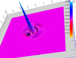
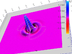
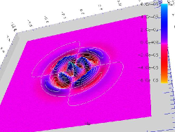
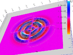
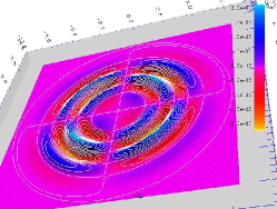
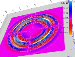
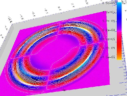
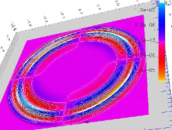
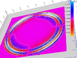
Figure 1: Evolution of the $h^{\varphi\varphi}$ component of $\bm{h}$ in the plane $\theta=\pi/2$, between $t=0$ (upper left) and $t=8r_{0}$ (lower right). The various snapshots are separated by a constant time interval $\Delta t=r_{0}$. The size of the depicted square is $16r_{0}$, so that the wave extraction surface at $R_{\rm ext}=8r_{0}$ is given by the circle inscribed in this square.

VI First results from a numerical implementation

VI.1 Short description of the code

We have implemented the constrained scheme given in Sec. V.5 in a numerical code designed to evolve vacuum spacetimes within maximal slicing and Dirac gauge. The code is constructed upon the C++ library Lorene Lorene . It uses multidomain spectral methods BonazGM98 ; BonazGM99b to solve the partial-differential equations within spherical coordinates. The scalar Poisson solver is that of Ref. GrandBGM01 , whereas the vector Poisson equation for the shift is solved via the method (ii) presented in Sec. V.2.2. The scalar wave equations for $\chi$ and $\mu$ [Eqs. (141) and (151)] are integrated forward in time by means of the technique presented in Ref. NovakB04 , namely a second-order semi-implicit Crank-Nicholson scheme with efficient outgoing-wave boundary conditions. By “efficient” we mean that all wave modes with spherical harmonics indices $\ell=0$, $1$ and $2$ are extracted at the outer boundary without any spurious reflection. This is far better than the Sommerfeld boundary condition commonly used in numerical relativity and which is valid only for the mode $\ell=0$.

Various concentric shell-like domains are used, the outermost one being compactified, to bring spatial infinity to the computational domain. The compactified domain is employed to solve all the elliptic equations, allowing for the correct asymptotic flatness boundary conditions. On the contrary, the wave equations are solved only in the non-compactified domains, the outgoing-wave boundary condition NovakB04 being imposed at the boundary between the last non-compactified shell and the compactified one. Further details upon the numerical code will be presented in a future publication.

VI.2 Initial data and computational setting

We have employed the code to evolve pure 3-D gravitational wave spacetimes, as in the two BSSN articles ShibaN95 ; BaumgS99 . Initial data have been obtained by means of the conformal thin sandwich formalism York99 ; PfeifY03 . The freely specifiable parameters of this formalism are $\bm{\tilde{\gamma}}$, ${\partial\bm{\tilde{\gamma}}/\partial t}$, $K$ and ${\partial K/\partial t}$. In accordance with our choice of maximal slicing, we set $K=0$ and ${\partial K/\partial t}=0$. Moreover, we use momentarily static data, ${\partial\bm{\tilde{\gamma}}/\partial t}=0$, along with a conformal metric $\bm{\tilde{\gamma}}$ resulting from

$$\chi(t=0) = {\chi_{0}\over 2}\,r^{2}\exp\left(-{r^{2}\over r_{0}^{2}}\right)\,\sin^{2}\theta\,\sin 2\varphi$$ (170)

$$\mu(t=0) = 0.$$ (171)

The constant numbers $\chi_{0}$ and $r_{0}$ parametrize respectively the amplitude and the width of the initial wave packet. Let us recall that, within Dirac gauge, the two scalars $\chi$ and $\mu$ fully specify $\bm{h}$ and thus $\bm{\tilde{\gamma}}$: $(\chi,\mu)$ determine a unique TT tensor $\bm{\bar{h}}$ according to the decomposition presented in Sec. V.3.2 and the full $\bm{h}$ is reconstructed from the trace $h$ computed in order to ensure $\det\tilde{\gamma}^{ij}=f^{-1}$, following the method given in Sec. V.4. It can be shown that the metric defined by Eq. (170)-(171) corresponds to an even-parity Teukolsky wave Teuko82 with $M=2$. These initial data are similar to those used by Baumgarte and Shapiro BaumgS99 except theirs correspond to a $M=0$ (axisymmetric) Teukolsky wave. In particular, we choose an amplitude $\chi_{0}=10^{-3}$ similar to that in Ref. BaumgS99 .

A total of 6 numerical domains have been used: a spherical nucleus of radius $r=r_{0}$, surrounded by 4 spherical shells of outer radius $r=2r_{0}$, $4r_{0}$, $6r_{0}$ and $8r_{0}$, and an external compactified domain of inner radius $r=8r_{0}$. The outgoing wave boundary conditions discussed above are set at $r=8r_{0}$, which we call the wave extraction radius $R_{\rm ext}$. In particular, this means that we do not solve for $\bm{h}$ for $r>8r_{0}$. Consequently we set $\bm{h}$ to zero in the region $r>8r_{0}$. More precisely, we perform a smooth matching of the value of $\bm{h}$ at $r=6r_{0}$ to zero at $r=8r_{0}$. This means that we solving all the Einstein equations only for $r<6r_{0}$. For $r\in[6r_{0},\infty)$ we are solving the Einstein equations only for the lapse $N$, the shift vector $\bm{\beta}$ and the conformal factor $\Psi$, with $\bm{h}$ set to zero in the $r>8r_{0}$ part of their source terms. We take into account the symmetries present in the initial data (170)-(171): (i) symmetry with respect to the plane $\theta=\pi/2$ and (ii) symmetry with respect to the transformation $\varphi\mapsto\varphi+\pi$. Accordingly, the computational coordinate $\theta$ spans the interval $[0,\pi/2]$ only and $\varphi$ the interval $[0,\pi)$. In each domain, the following numbers of collocations points (= numbers of polynomials in the spectral expansions) are used: $N_{r}\times N_{\theta}\times N_{\varphi}=17\times 9\times 8$. The corresponding memory requirement is 260 MB. This modest value allows the computation to be performed on a laptop. We have used two different time steps $\delta t=10^{-2}r_{0}$ and $\delta t=5\,10^{-3}r_{0}$, to investigate the effects of time discretization.

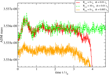
Figure 2: Evolution of the ADM mass for three different computational settings, corresponding to different values of the time step $\delta t$ and the wave extraction radius $R_{\rm ext}$.

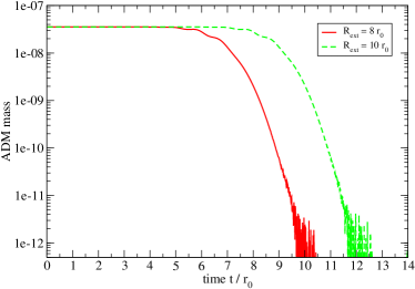
Figure 3: Evolution of the ADM mass (logarithmic scale, contrary to Fig. 2) for two different values of the wave extraction radius $R_{\rm ext}$.

VI.3 Results

The time evolution of the component $h^{\varphi\varphi}$ of $\bm{h}$ is shown in Fig. 1. All the wave packet leaves the computational domain $r<8r_{0}$ around $t\sim 8r_{0}$ and we do not notice on Fig. 1 any spurious reflexion.

In order to test the code, we have monitored the ADM mass defined by

$$M_{\rm ADM}={1\over 16\pi}\oint_{\infty}\left[{\cal D}^{j}\gamma_{ij}-{\cal D}_{i}\left(f^{kl}\gamma_{kl}\right)\right]dS^{i},$$ (172)

where the integral is taken over a sphere of radius $r=+\infty$ and where we have adapted the original definition ArnowDM62 to general coordinates (i.e. non asymptotically Cartesian) by the explicit introduction of the flat metric $\bm{f}$. The above integral can be re-written in terms of the conformal metric and conformal factor:

$$M_{\rm ADM}=-{1\over 16\pi}\oint_{\infty}\left(8{\cal D}_{i}\Psi+f_{ij}{\cal D}_{k}h^{jk}-{\cal D}_{i}h\right)dS^{i}.$$ (173)

Within Dirac gauge, the second term in the integrand vanishes identically, whereas the last one does not contribute to the integral, due to the fast decay of $h$ (at least $O(r^{-2})$) implied by Eq. (169). Therefore the expression for the ADM mass reduces to the flux of the gradient of the conformal factor:

$$M_{\rm ADM}=-{1\over 2\pi}\oint_{\infty}{\cal D}_{i}\Psi\,dS^{i}.$$ (174)

Hence the expression of ADM mass in Dirac gauge is identical to the well known expression for conformally flat hypersurfaces. The evolution of the ADM mass computed by means of Eq. (174) (let us recall that the sphere at $r=\infty$ belongs to our computational domain) is presented in Fig. 2. For $t<3r_{0}$, one sees that the ADM mass is conserved, as it should be, with an accuracy of four digits. Moreover, Fig. 2 shows that the main source of error in the ADM mass is the finite value of the time step $\delta t$. For $t>3r_{0}$, the ADM mass starts to decrease, reflecting the fact that that the wave is leaving the domain $r\leq R_{\rm ext}$. Note that by increasing the wave extraction radius from $R_{\rm ext}=8r_{0}$ to $R_{\rm ext}=10r_{0}$, we get a conservation of the ADM mass up to $t\simeq 5r_{0}$ (dashed curved in Fig. 2). In Fig. 3, we present the evolution of the ADM mass on a longer timescale. We see clearly that, after remaining constant (the part shown in Fig. 2), the ADM mass decreases by four orders of magnitude after $t\simeq 10r_{0}$ (resp. $t\simeq 12r_{0}$) for the wave extraction radius $R_{\rm ext}=8r_{0}$ (resp. $R_{\rm ext}=10r_{0}$). The very small value of the ADM mass at late times demonstrates that all the wave packet has leaved the domain $r\leq R_{\rm ext}$ and no spurious reflection has occurred. This is due to the efficient outgoing wave boundary conditions NovakB04 set at the wave extraction radius.

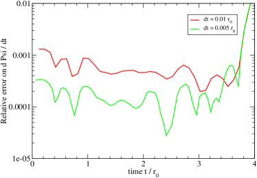
Figure 4: Relative error $\varepsilon$ [Eq. (175)] on the time derivative of the conformal factor $\Psi$ in the central domain ($r\leq r_{0}$).

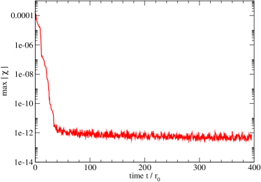
Figure 5: Evolution of the maximum of absolute value of the potential $\chi$ [Eq. (140)] for the long term run.

Another test is provided by Eq. (75) which relates the time derivative of the conformal factor $\Psi$ to the divergence of the shift vector $\bm{\beta}$. As mentioned in Sec. V.5, this equation must hold but is not enforced in our scheme. In a given numerical domain we define the relative error on Eq. (75) by

$$\varepsilon:={\left|{\partial\Phi/\partial t}-\beta^{k}{\cal D}_{k}\Phi-{1\over 6}{\cal D}_{k}\beta^{k}\right|\over{\rm max}\left|{\partial\Phi/\partial t}\right|+{\rm max}\left|\beta^{k}{\cal D}_{k}\Phi+{1\over 6}{\cal D}_{k}\beta^{k}\right|},$$ (175)

where the max are taken on the considered domain. We represent the value of $\varepsilon$ in the domain where it is the largest, namely the nucleus ($r\leq r_{0}$), in Fig. 4. We see that Eq. (75) is actually very well satisfied. The error is in fact dominated by the time discretization (second order scheme), and is as low as a few $10^{-4}$ for $\delta t=5\;10^{-3}r_{0}$. The increase of $\varepsilon$ at $t\sim 4r_{0}$ is spurious and is due to the arrival of the wave packet in the wave extraction domain $6r_{0}\leq r\leq 8r_{0}$.

To check the long term stability of the code, we have let it run well after the wave packet has leaved the area $r<8r_{0}$, namely until $t=400r_{0}$. This very long time scale is similar with that used in Ref. BaumgS99 to assess the stability of the BSSN scheme. We found no instability to develop. In particular the maximum value of the potential $\chi$ remains at the round-off error value of $10^{-12}$ that has been reached at $t\sim 40r_{0}$ (see Fig. 5).

VII Summary and conclusions

We have introduced on each hypersurface $t={\rm const}$ of the 3+1 formalism a flat 3-metric $\bm{f}$, in addition to the (physical) 3-metric $\bm{\gamma}$ induced by the spacetime 4-metric $\bm{g}$, in such a way that asymptotically both metrics coincide. This allows us to define properly the conformal metric $\bm{\tilde{\gamma}}$ and not to stick to Cartesian coordinates. A flat metric is introduced anyway, more or less explicitly, when performing numerical computations. We have written the 3+1 equations entirely in terms of the covariant derivative associated with the flat metric $\bm{f}$.

The Dirac gauge is expressed simply in terms of this flat metric as the vanishing of the divergence with respect to $\bm{f}$ of the conformal metric $\bm{\tilde{\gamma}}$. Moreover in spherical components, the Dirac gauge reduces the resolution of the equations for $\bm{\tilde{\gamma}}$ to two scalar wave equations. The remaining four components $\tilde{\gamma}^{ij}$ are then obtained from the condition $\det\tilde{\gamma}^{ij}=\det f^{ij}$ and the three components of the Dirac condition ${\cal D}_{j}\tilde{\gamma}^{ij}=0$. This clearly shows that the gravitational field has two degrees of freedom and this exhibits the TT wave behavior of the metric at infinity. Let us stress that the usage of spherical coordinates and spherical components is essential for the reduction to two scalar wave equations. To our knowledge, this is the first time that a differential gauge is used to directly compute some of the metric components, thus decreasing the number of PDE to be solved. Previously, this was done only for algebraic gauges (i.e. setting some of the metric components to zero).

Contrary to e.g. the minimal distortion gauge SmarrY78a or the “Gamma-driver” gauge AlcubB01 , the Dirac gauge completely fix the coordinates (up to some boundary conditions) in the initial hypersurface $\Sigma_{0}$. This implies that initial data must be prepared within this gauge, which might be regarded as a drawback (for instance an analytic expression for the Kerr solution is not known in Dirac gauge). On the contrary, an advantage of the full coordinate fixing is to allow to compute stationary solutions by simply setting ${\partial/\partial t}=0$ in the various equations. For instance, Shibata, Uryu and Friedman ShibaUF04 have recently proposed to use the Dirac gauge to compute quasiequilibrium configurations of binary neutron stars.

In addition to the Dirac gauge, the use of the maximal slicing results in an elliptic equation for the lapse function. Another elliptic equation for the conformal factor $\Psi$ (or equivalently for $Q:=\Psi^{2}N$) arises from the Hamiltonian constraint. The Dirac gauge itself, in conjunction with the momentum constraint, results in an elliptic equation for the shift $\bm{\beta}$. The maximal slicing relates the divergence of $\bm{\beta}$ to the time derivative of the conformal factor.

Solving the above equations implies that the four constraints are fulfilled by the solution. As already mentioned in the Introduction, some authors have proposed very recently a scheme in which the constraints, re-written as time evolution equations, are satisfied up to the time discretization errors GentlGKM03 . On the contrary, in our scheme the constraints are fulfilled within the precision of the space discretization errors (which can be very low with a modest computational cost, thanks to spectral methods).

It is worth noticing that the five elliptic equations of the widely used Isenberg-Wilson-Mathews approximation to General Relativity Isenb78 ; IsenbN80 ; WilsoM89 (see also Ref. FriedUS02 ) are naturally recovered in our scheme by simply setting $\bm{h}=0$: they are the equations for $N$, $Q$ and $\bm{\beta}$.

We have demonstrated the viability of the proposed constrained scheme by numerically computing the evolution of a gravitational wave packet in a vacuum spacetime. The numerical evolution has been found to be both very accurate and stable. We are also made confident by existing constrained schemes for vector equations which have proved to be successful: the divergence-free hydro scheme of Ref. VillaB02 (the constraint being that the velocity field is divergence-free) and some MHD schemes in cylindrical coordinates KeppeT99 (the constraint being that the magnetic field is divergence-free).

In this paper we have focused on space slices with $\mathbb{R}^{3}$ topology, except for Appendix A where we briefly discuss the properties of degenerate second order operators and the number of boundary conditions at the surface of excised holes with vanishing lapse. In a future work, we shall focus on black hole spacetimes.

Appendix A Degenerate elliptic operators on a black hole horizon

In our view, a numerical scheme for black hole spacetimes should recover known stationary solutions in coordinate-time independent form (i.e. with the $\partial/\partial t$ coordinate vector coinciding with the Killing vector of stationarity). Indeed we require arbitrary long term evolution of steady state, or quasi-steady state, black hole spacetimes. For classical solutions (Kerr) in usual coordinates, this requirement results in a vanishing lapse on the horizon (see discussion in Refs. GourgGB02 ; HannaECB03 ). Therefore we excise from our computational domain a sphere $\cal H$ (or two spheres for binary systems) with $N=0$ as a boundary condition on that sphere and choose spherical coordinates such that $r=1$ on $\cal H$ .

In this case, the spatial operator acting on $\bm{h}$ in Eq. (85) must not be merely the Laplacian $\Delta$ but

$$\blacktriangle h^{ij}:=N\Delta h^{ij}-{\cal D}_{k}N\left({\cal D}^{i}h^{jk}+{\cal D}^{j}h^{ik}-{\cal D}^{k}h^{ij}\right).$$ (176)

This operator is formed by writing ${\cal D}_{k}Q=\Psi^{2}{\cal D}_{k}N+2N\Psi{\cal D}_{k}\Psi$ in the right-hand side of Eq. (85) and gathering the ${\cal D}_{k}N$ term with the $\Delta h^{ij}$ one. The operator $\blacktriangle$ is degenerate, because of the vanishing of $N$ at the boundary $\cal H$. Similarly, the operator acting on the shift vector $\bm{\beta}$ is degenerate on $\cal H$ (cf. Eq. (74) with $A^{ij}$ given by Eq. (92) which contains a division by the lapse $N$). Letting the unknown $u$ be a component of $h^{ij}$ or $\beta^{i}$, these equations are of the kind

$$N\Delta u+\epsilon\,{\cal D}_{i}N{\cal D}^{i}u=S,$$ (177)

with the associated homogeneous equation

$$N\Delta u+\epsilon\,{\cal D}_{i}N{\cal D}^{i}u=0,$$ (178)

where $N=0$ and $\partial N/\partial r>0$ at $r=1$, $\epsilon=\pm 1$ and $S$ is some effective source. Since Eq. (177) is linear, a solution is a linear combination of a particular solution and a homogeneous solution, i.e. a solution of Eq. (178). In the non-degenerate case, since Eq. (178) is of second order, we have two independent homogeneous solutions, which allow us to impose two boundary conditions. In the degenerate case ($N=0$ at $r=1$), the number of regular homogeneous solutions depends upon the sign of $\epsilon$: two for $\epsilon=-1$ and only one for $\epsilon=+1$. To illustrate this, let us consider the following one-dimensional second order equation analogue to Eq. (178) with $x=r-1$:

$$x{d^{2}u\over dx^{2}}+\epsilon{du\over dx}=0,\qquad\mbox{with}\ x\in[0,1].$$ (179)

The involved second-order operator is clearly degenerate at $x=0$. For $\epsilon=-1$, we have two independent homogeneous solutions:

$$u_{1}(x)={\rm const}\qquad\mbox{and}\qquad u_{2}(x)=x^{2},$$ (180)

whereas for $\epsilon=1$, the two independent homogeneous solutions are

$$u_{1}(x)={\rm const}\qquad\mbox{and}\qquad u_{2}(x)=\ln x.$$ (181)

The last one is clearly not regular at $x=0$, so that in this case, one can use only one homogeneous solution to satisfy a Dirichlet boundary condition.

This behavior of the degenerate operator can also be understood by considering the parabolic (heat-like) equation associated with Eq. (178):

$${\partial u\over\partial t}=N\Delta u+\epsilon\,{\cal D}_{i}N{\cal D}^{i}u.$$ (182)

The solution of the elliptic equation (178) is the eigenfunction corresponding to the zero eigenvalue of the spatial operator acting on the right-hand side of Eq. (182). In other words, the solution $u$ we search for is the relaxed solution of the heat-like equation (182). When $N\rightarrow 0$, Eq. (182) becomes an advection equation near $r=1$, for which the number of boundary conditions at $r=1$ is zero or one depending whether the “effective velocity” $-\epsilon\,{\cal D}_{i}N=-\epsilon\,{\partial N\over\partial r}\bm{e}_{r}$ is ingoing or outgoing at the boundary $r=1$.

For the spherical components of the shift vector, we have $\epsilon=-1$, so that a boundary condition can always be given at $r=1$, in addition to the boundary condition at $r=\infty$. Regarding the spherical components of the metric potential $h^{ij}$, $\epsilon=1$ for $h^{rr}$, which means that no boundary condition can be set at $r=1$ in addition to $h^{rr}=0$ at $r=\infty$. On the contrary, $\epsilon=-1$ for the potential $\mu$ introduced in Eqs. (144)-(145). These points shall be studied more in details in a future work. It is worth to mention that the boundary conditions for $h^{ij}$ at $r=1$ determine fully the coordinates within the Dirac gauge.

References

- (1) T.W. Baumgarte and S.L. Shapiro, Phys. Rep. 376, 41 (2003).
- (2) L. Lehner, Class. Quantum Grav. 18, R25 (2001).
- (3) J.W. York, in Sources of Gravitational Radiation, edited by L.L. Smarr (Cambridge University Press, Cambridge, 1979), p. 83.
- (4) J.M. Bardeen and T. Piran, Phys. Rep. 96, 205 (1983).
- (5) R.F. Stark and T. Piran, Phys. Rev. Lett. 55, 891 (1985).
- (6) C.R. Evans, in Dynamical Spacetimes and Numerical Relativity, edited by J. Centrella (Cambridge University Press, Cambridge, 1986).
- (7) C.R. Evans, in Frontiers in Numerical Relativity, edited by C.R. Evans, L.S. Finn, and D.W. Hobill (Cambridge University Press, Cambridge, 1989), p. 194.
- (8) S.L. Shapiro and S.A. Teukolsky, Phys. Rev. D 45, 2739 (1992).
- (9) A.M. Abrahams, G.B. Cook, S.L. Shapiro, and S.A. Teukolsky, Phys. Rev. D 49, 5153 (1994).
- (10) M.W. Choptuik, E.W. Hirschmann, S.L. Liebling, and F. Petrorius, Class. Quantum Grav. 20, 1857 (2003).
- (11) M. Anderson and R.A. Matzner, preprint gr-qc/0307055.
- (12) H. Shinkai and G. Yoneda, to appear in Progress in Astronomy and Astrophysics (Nova Science Publ.), preprint gr-qc/0209111.
- (13) L. Lindblom, M.A. Scheel, L.E. Kidder, H.P. Pfeiffer, D. Shoemaker, and S.A. Teukolsky, Phys. Rev. D 69, 124025 (2004).
- (14) M. Shibata and T. Nakamura, Phys. Rev. D 52, 5428 (1995).
- (15) T.W. Baumgarte and S.L. Shapiro, Phys. Rev. D 59, 024007 (1999).
- (16) M. Shibata and K. Uryu, Phys. Rev. D 61, 064001 (2000).
- (17) M. Shibata and K. Uryu, Phys. Rev. D 64, 104017 (2001).
- (18) S. Bonazzola and J.-A. Marck, J. Comput. Phys. 87, 201 (1990).
- (19) P. Grandclément, S. Bonazzola, E. Gourgoulhon, and J.-A. Marck, J. Comput. Phys. 170, 231 (2001).
- (20) A.P. Gentle, N.D. George, A. Kheyfets, and W.A. Miller, Class. Quantum Grav. 21, 83 (2004).
- (21) P.A.M. Dirac, Phys. Rev. 114, 924 (1959).
- (22) S. Deser, Int. J. Mod. Phys. A 19S1, 99 (2004).
- (23) L. Smarr and J.W. York, Phys. Rev. D 17, 1945 (1978).
- (24) E. Gourgoulhon, P. Grandclément, K. Taniguchi, J.-A. Marck, and S. Bonazzola, Phys. Rev. D 63, 064029 (2001).
- (25) P. Grandclément, E. Gourgoulhon, and S. Bonazzola, Phys. Rev. D 65, 044021 (2002).
- (26) S. Bonazzola, E. Gourgoulhon, and J.-A. Marck, Phys. Rev. D 58, 104020 (1998).
- (27) J. Novak and S. Bonazzola, J. Comput. Phys. 197, 186 (2004).
- (28) E. Gourgoulhon, P. Grandclément, and S. Bonazzola, Phys. Rev. D 65, 044020 (2002).
- (29) M.D. Hannam, C.R. Evans, G.B. Cook, and T.W. Baumgarte, Phys. Rev. D 68, 064003 (2003).
- (30) T. Nakamura, K. Oohara, and Y. Kojima, Prog. Theor. Phys. Suppl. 90, 1 (1987).
- (31) S.R. Brandt and E. Seidel, Phys. Rev. D 52, 856 (1995).
- (32) S.R. Brandt and E. Seidel, Phys. Rev. D 52, 870 (1995).
- (33) R.F. Stark, in Frontiers in Numerical Relativity, edited by C.R. Evans, L.S. Finn, and D.W. Hobill (Cambridge University Press, Cambridge, 1989), p. 281.
- (34) S. Bonazzola, E. Gourgoulhon, and J.-A. Marck, J. Comput. Applied Math. 109, 433 (1999).
- (35) H.P. Pfeiffer, L.E. Kidder, M.A. Scheel, and S.A. Teukolsky, Comput. Phys. Commun. 152, 253 (2003).
- (36) H. Dimmelmeier, J.A. Font, and E. Mueller, Astron. Astrophys. 388, 917 (2002).
- (37) H. Dimmelmeier, J. Novak, J.A. Font, J.Ma. Ibáñez, and E. Mueller, preprint astro-ph/0407174.
- (38) J.W. York, Phys. Rev. Lett. 28, 1082 (1972).
- (39) M. Alcubierre, B. Brügmann, P. Diener, M. Koppitz, D. Pollney, E. Seidel, and R. Takahashi, Phys. Rev. D 67, 084023 (2003).
- (40) J.W. York, Phys. Rev. Lett. 82, 1350 (1999).
- (41) M. Alcubierre, G. Allen, B. Brügmann, E. Seidel, and W.-M. Suen, Phys. Rev. D 62, 124011 (2000).
- (42) M. Alcubierre, B. Brügmann, M. Miller, and W.-M. Suen, Phys. Rev. D 60, 064017 (1999).
- (43) A. Lichnerowicz, J. Math. Pures Appl. 23, 37 (1944).
- (44) L. Smarr and J.W. York, Phys. Rev. D 17, 2529 (1978).
- (45) T. Nakamura, in Relativistic Cosmology, Proceedings of the 8th Nishinomiya-Yukawa Memorial Symposium, edited by M. Sasaki (Universal Academy Press, Tokyo, 1994), p. 155.
- (46) M. Kawamura, K. Oohara and T. Nakamura, Prog. Theor. Phys., submitted, preprint astro-ph/0306481.
- (47) M. Shibata, K. Uryu and J.L. Friedman, Phys. Rev. D, in press, preprint gr-qc/0407036.
- (48) L. Andersson and V. Moncrief, Ann. Henri Poincaré 4, 1 (2003).
- (49) R. Arnowitt, S. Deser, and C.W. Misner, in Gravitation: an introduction to current research, edited by L. Witten (Wiley, New York, 1962), p. 277.
- (50) K.S. Thorne, Rev. Mod. Phys. 52, 299 (1980).
- (51) J. Matthews, J. Soc. Ind. Appl. Math. 10, 768 (1962).
- (52) F.J. Zerilli, J. Math. Phys. 11, 2203 (1970).
- (53) T. Regge and J.A. Wheeler, Phys. Rev. 108, 1063 (1957).
- (54) S.A. Teukolsky, Phys. Rev D 26, 745 (1982).
- (55) P.M. Morse and H. Feshbach, Methods of theoretical physics, McGraw-Hill, New York (1953).
- (56) L. Villain and S. Bonazzola, Phys. Rev. D 66, 123001 (2002).
- (57) http://www.lorene.obspm.fr
- (58) H.P. Pfeiffer and J.W. York, Phys. Rev. D 67, 044022 (2003).
- (59) M. Alcubierre and B. Brügmann, Phys. Rev. D 63, 104006 (2001).
- (60) J. A. Isenberg : Waveless approximation theories of gravity, preprint University of Maryland, unpublished (1978).
- (61) J. Isenberg and J. Nester, in General Relativity and Gravitation, edited by A. Held (Plenum, New York, 1980), Vol. 1.
- (62) J. R. Wilson and G. J. Mathews, in Frontiers in numerical relativity, edited by C. R. Evans, L. S. Finn and D. W. Hobill (Cambridge University Press, Cambridge, England, 1989).
- (63) J. L. Friedman, K. Uryu, and M. Shibata, Phys. Rev. D 65, 064035 (2002).
- (64) R. Keppens and G. Tóth, Phys. Plasma 6, 1461 (1999).