The naked singularity in the global structure of critical collapse spacetimes

Abstract

We examine the global structure of scalar field critical collapse spacetimes using a characteristic double-null code. It can integrate past the horizon without any coordinate problems, due to the careful choice of constraint equations used in the evolution. The limiting sequence of sub- and supercritical spacetimes presents an apparent paradox in the expected Penrose diagrams, which we address in this paper. We argue that the limiting spacetime converges pointwise to a unique limit for all $r>0$, but not uniformly. The $r=0$ line is different in the two limits. We interpret that the two different Penrose diagrams differ by a discontinuous gauge transformation. We conclude that the limiting spacetime possesses a singular event, with a future removable naked singularity.

I Introduction

The critical collapse of scalar fields gives rise to a new class of thought experiments in general relativity Choptuik:1993jv ; Gundlach:2002sx . It has been suggested that a weak singularity may be visible to a distant observer during the collapse of a scalar field Israel:1986 ; Burko:1998az . With the presence of such potentially problematic phenomena, one can ask to what degree cosmic censorship is violated. The spirit of the cosmic censorship conjecture is that the evolution of spacetimes as seen by distant observers in asymptotically flat regions is determined uniquely by the Einstein equations. If visible infinite curvature arises in the evolution from regular initial data, one might have cause for concern about the classical completeness of Einstein’s theory of gravity. The critical collapse is a fine-tuned limit, and “strong cosmic censorship” has been formulated to exclude such rare cases with zero measure in the space of initial conditions. It is nevertheless instructive to understand the nature of this singularity, and how such a limit can be taken.

Recently, Martin-Garcia and Gundlach Martin-Garcia:2003gz have numerically constructed a self-consistent discretely self-similar spacetime which they argued to be related to the evolutionary critical collapse solutions. They proposed the existence of a future Cauchy horizon emanating from the critical collapse event, on which new data must be specified. The authors proceeded to find a unique way of specifying this data which can result in a regular future spacetime.

In this paper, we consider the problem from a different perspective. Instead of searching for the critical solution of Einstein equations by first taking the limit of discrete self-similarity, we study the constructive sequence of non-critical global spacetimes. We then search for a unique limit as we approach criticality. Posed in such a way, the existence of a Cauchy horizon would be very unexpected: each spacetime in the limit sequence has no Cauchy horizon, so why would it form in the limit? To study the problem, we developed a characteristic code which can track a scalar field collapse interior to the horizon. In Section II, we outline a conceptual paradox in the search for a global critical spacetime structure. In Section III, we derive the scalar field equations of motion with spherical symmetry. We proceed to solve these equations numerically in Section IV. The numerical results are presented in Section V, where we explain our proposed solution to the apparent paradox.

II The apparent paradox

Consider a collapsing scalar field with amplitude characterized by a parameter $p$. For small amplitudes $p<p_{*}$, the field collapses and re-expands. For large amplitudes $p>p_{*}$, a black hole forms. An interesting question is to examine the behavior when $p=p_{*}$. One can consider two limits, one from below and one from above. If we consider a sequence of subcritical spacetimes with collapsing scalar fields as they approach $p_{*}$ from below, we might expect the global structure of the resulting spacetime to be Minkowski, i.e. a triangle shown in the left panel of Fig. 1. If we consider the limit of a sequence of supercritical spacetimes from above, we expect each stage to have a global Schwarzschild structure. As the parameter decreases, the mass of the resulting black hole approaches zero, and one expects the limiting spacetime to resemble a Schwarzschild spacetime with zero mass, shown in the right panel of Fig. 1. In this limit, $r=0$ coincides with the horizon and becomes null (and infinitely redshifted). The global structure looks quadrangular, quite unlike the argued spacetime in the other limit.

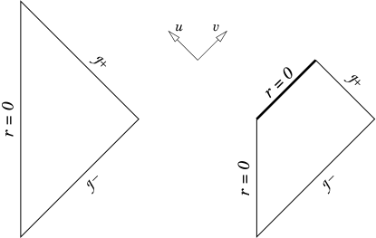
Figure 1: Two possible global structures of a critical collapse spacetime. The left is the diagram expected taking a limit of subcritical collapses, while the right diagram is a zero mass black hole resulting from the limit sequence of supercritical collapse.

This suggests several possible interpretations. Perhaps the two limits are different, and the limiting spacetime depends on the direction from which the limit was taken. Or one of the limits is only an incomplete description of spacetime, and might be extensible to the same global structure. Or perhaps the limit is not convergent from either direction, and oscillates in such a way that more data must be specified on a spontaneously formed Cauchy horizon Martin-Garcia:2003gz . Our study suggests a slightly different physical interpretation of the global structure.

Critical spacetimes are only known as numerical solutions, which makes questions about global structure hard to answer. It is most easily studied in characteristic coordinates which follow light ray propagation Garfinkle:1995jb . In the subsequent section we will describe our formulation and implementation of the numerical procedures.

III Spherically Symmetric Scalar Field Collapse

The spherically symmetric $(n+2)$-dimensional spacetime metric can be written as

$$ds^{2}=e^{-2\sigma}d\vec{x}^{2}+e^{2\mu}d\Omega^{2},$$ (1)

where $d\Omega^{2}$ is the metric of a unit $n$-dimensional sphere with curvature $K=1$, and the two-manifold metric $d\gamma^{2}=e^{-2\sigma}d\vec{x}^{2}$ is conformally flat. The dynamics of the scalar field collapse are described by the reduced action

$$S \propto \int d^{2}x\,e^{n\mu}\Big{\{}-2(\nabla\phi)^{2}-2n(\nabla\sigma\cdot\nabla\mu)$$

$$\hskip 50.00008pt+n(n-1)\left[(\nabla\mu)^{2}+Ke^{-2(\sigma+\mu)}\right]\Big{\}},$$

where integration and differential operators are with respect to the flat two-metric $d\vec{x}^{2}$. Variation of the above action with respect to the fields $\phi$, $\mu$ and $\sigma$ gives equations of motion

$$\Box\phi+n(\nabla\mu\cdot\nabla\phi)=0,$$ (3a)

$$\Box\mu+n(\nabla\mu)^{2}-(n-1)Ke^{-2(\sigma+\mu)}=0,$$ (3b)

$$\Box\sigma-\frac{n}{2}\left\{\Box\mu+(\nabla\mu)^{2}\right\}-(\nabla\phi)^{2}=0,$$ (3c)

while the two constraint equations are recovered by variation with respect to the (flat) metric

$$\text{Traceless}\left\{\mu_{;ab}+\mu_{,a}\mu_{,b}+2\mu_{(,a}\sigma_{,b)}+{\textstyle\frac{2}{n}}\phi_{,a}\phi_{,b}\right\}=0.$$ (4)

For the particular case of spherically symmetric scalar field collapse in four dimensions ($n=2$), the equations of motion (3) can be simplified by introducing auxiliary field variables $r=e^{\mu}$ and $\varphi=r\phi$:

$$\Box(r^{2})=2e^{-2\sigma},$$ (5a)

$$\Box\varphi=\frac{\Box r}{r}\,\varphi,$$ (5b)

$$\Box\sigma=\frac{\Box r}{r}+(\nabla\phi)^{2}.$$ (5c)

This form of the dynamical equations is better suited for numerical evolution.

IV Characteristic Code

We discretize and evolve the collapsing scalar field spacetime in double-null coordinates $d\vec{x}^{2}=-2\,du\,dv$, where the radial characteristics of the wave equations are made explicit: the outgoing characteristic propagates at constant $u$ in the direction of increasing $v$, while the incoming characteristic propagates at constant $v$ in the direction of increasing $u$. This approach has a number of advantages over some of the more traditional spacetime slicings.

The characteristic code only propagates information along characteristics at a numerical speed equal to the true characteristic speed. The numerical domain of dependence is no larger than the physical domain of dependence, and the code still maintains full (second order) accuracy. Horizons are not particularly special as far as ingoing null characteristics are concerned. This allows us to follow collapse all the way to the singularity. Even as an outgoing characteristic hits a singularity and the floating point numbers denormalize, this does not affect any of the other characteristics, which can be integrated to fill the whole maximally extended spacetime determined by the initial data. To illustrate this point, in Fig. 2 we present Penrose and Kruskal diagrams of a spacetime with a large black hole formed in the collapse of the scalar field wavepacket.

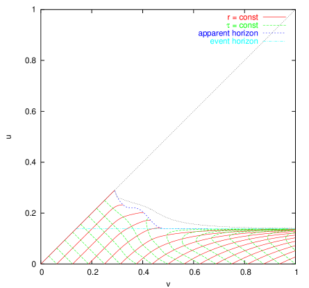
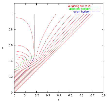
Figure 2: Penrose (left) and Kruskal (right) style diagrams of the spacetime with a large black hole produced in the collapse of a sine-squared scalar field wavepacket (14). The grid lines on the Penrose diagram show observers at constant radius and the proper time according to their clocks (note that the plot is rotated $45^{\circ}$ compared to Fig. 1; the diagonal line $u=v$ is the origin $r=0$). The Kruskal diagram shows the trajectories of outgoing null rays as emitted from the center of spacetime at subsequent moments of time. The code sees both real and apparent horizons, as well as the formation of the spacelike singularity (small region around which is excised). Note that the apparent and event horizons are not the same, as the spacetime is not static.

The two-dimensional metric $d\gamma^{2}$ has a residual gauge freedom under redefinition of the null coordinates $u\mapsto U(u)$, $v\mapsto V(v)$. These two free functions (of a single variable) are used to define the coordinate $v$ on the initial slice and to map the central point $r=0$ to a straight line in the $(u,v)$ plane:

$$v|_{u=0}=\sqrt{2}\,r,\hskip 10.00002ptu|_{r=0}=v.$$ (6)

The second gauge condition is particularly convenient, since it places the central point at a known location on the grid when discretizing.

The initial conditions are specified on a surface of constant $u$ by giving a scalar field profile $\phi(v)$. Together with the gauge choice (6), this determines the rest of the variables. In particular, $\sigma(v)$ is obtained by integrating the outgoing ($vv$) constraint equation (4)

$$\sigma|_{u=0}=-\frac{1}{2}\int\phi_{,v}^{2}vdv.$$ (7)

The integration is implemented as a fourth order Runge-Kutta algorithm with a fixed step. Although strictly speaking it is not necessary, as the evolution code is second order, it is no more complicated than a second order integrator would be.

Although the constraint equations follow from the dynamical equations, their use might be required for stability Gundlach:1997rk . Using the outgoing constraint equation for evolution (rather than just for initial conditions) is not a good idea, however. It becomes degenerate on the apparent horizon, where the outgoing light rays become (marginally) trapped $r_{,v}=0$. The incoming constraint equation is perfectly fine, though, and could be followed all the way to the center of the spacetime, whether it is singular or not. By introducing an auxiliary field variable $\tau=\sigma+\frac{1}{2}\ln\left(-\sqrt{2}\,r_{,u}\right)$, the incoming constraint equation (4) can be written in a form that is very simple to integrate

$$\tau_{,u}=-\frac{1}{2}\frac{\phi_{,u}^{2}}{(\ln r)_{,u}}.$$ (8)

To integrate the incoming constraint, one would need to know the values of $\tau$ on the initial slice $u=\text{const}$. These can be found by integration of the equation

$$\tau_{,v}=-\frac{1}{2}\phi_{,v}^{2}v-\frac{1}{2v}\left[1-e^{-2\tau}\right],$$ (9)

which is obtained by combining the constraints with the evolution equation (5a) to solve for $r_{,u}$ on the initial slice.

Having discussed our gauge choice, initial conditions and constraint equations, we now come to the discretization of the evolution equations. The covariant differential operators in the evolution equations (5) are with respect to a flat metric, so in null coordinates they are written simply as

$$\Box x=-2\partial_{u}\partial_{v}x,\hskip 10.00002pt(\nabla x)^{2}=-2(\partial_{u}x)(\partial_{v}x),$$ (10)

where $x$ denotes any one of the three dynamical variables in equations (5). We discretize by finite differencing on a rectilinear $(u,v)$ grid with equal spacing $du=dv=\Delta$, which to second order accuracy gives

$$(\Box x)_{\times} = -\frac{2}{\Delta^{2}}\left[x_{++}+x_{--}-x_{+-}-x_{-+}\right],$$ (11)

$$(\nabla x)^{2}_{\times} = -\frac{1}{2\Delta^{2}}\left[(x_{++}-x_{--})^{2}-(x_{-+}-x_{+-})^{2}\right],$$

where the differential operators are evaluated at the center of a grid cell (see Fig. 3).

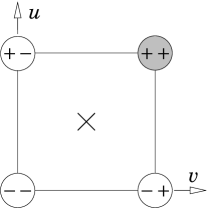
Figure 3: Discretization on a $(u,v)$ grid.

The code takes a step by using discretized evolution equations to find the values of the fields at the $(++)$ grid point (shaded node in Fig. 3). The only non-trivial operation involved in this is finding $r_{++}$ accurate to second order, which is done by solving equation (5a) discretized in the following fashion:

$$r_{++}^{2}+r_{--}^{2}-r_{+-}^{2}-r_{-+}^{2}=$$ (12)

$$\hskip 10.00002pt\frac{\Delta}{\sqrt{2}}\exp(-\tau_{+-}-\tau_{-+})(r_{++}+r_{+-}-r_{-+}-r_{--}).$$

The rest is then straightforward, as the right hand sides of equations (5b,c) become known.

As the code advances to the next slice of constant $u$, the very first point on the grid ($u=v$) is the center of the spacetime ($r=0$) and has to be treated specially. The asymptotic form of the evolution equations at $r=0$

$$\textstyle\nabla r\cdot\nabla\phi=0,\hskip 10.00002pt\sigma=-\frac{1}{2}\ln(\nabla r)^{2}$$ (13)

is used to calculate the values of the fields in the center.

V Results

We tested the code on the collapse of a scalar field with various initial conditions. In particular, we used pulse

$$\phi(v)=\left\{\begin{array}[]{cc}p\sin^{2}4\pi v,&\frac{1}{4}<v<\frac{1}{2}\\ 0&\text{otherwise}\\ \end{array}\right.$$ (14)

and kink

$$\phi(v)=\left\{\begin{array}[]{cc}p+p\tanh\left[5\tan\pi(\frac{4}{3}v-\frac{1}{2})\right],&v<\frac{3}{4}\vskip 3.0pt plus 1.0pt minus 1.0pt\\ 2p,&v\geq\frac{3}{4}\\ \end{array}\right.$$ (15)

field profiles in our simulations. Both profiles are fairly smooth functions with field energy density having compact support on the initial slice. This avoids the interference of long-range tails in the initial data on the late-time evolution.

All runs shown in this paper used 65536 uniformly spaced grid points. The critical scaling of black hole mass is shown in Fig. 4. It agrees well with the literature Choptuik:1993jv ; Hod:1997az . Our achievable dynamic range shows scaling over three orders of magnitude in black hole mass without the use of adaptive mesh refinement. This is sufficient for our study. Further improvements in dynamic range can be sought after using adaptive mesh refinement techniques or adopting an initial gauge which places ingoing null rays on a grid more densely near the collapse point Garfinkle:1995jb . As the grid resolution is increased, the double arithmetic precision and round-off errors become the main obstacles in the quest for higher dynamical range.

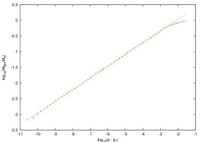
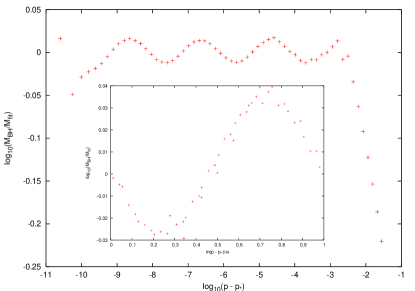
Figure 4: Black hole mass scaling for single kink wave, given by equation (15). The upper panel shows a power law fit to the numerical data with critical exponent $\gamma\approx 0.373$ which holds over three orders of magnitude in black hole masses, corresponding to nine orders of magnitude in the tuning parameter. The lower panel shows the residual after the power law fit, demonstrating periodic fine structure due to discrete self-similarity of the collapse. Its period $\omega\approx 4.63$ corresponds to the value of the echoing parameter $\Delta\approx 3.45$. The lower panel inset shows the residual mapped to a single period (outlier points removed), illustrating that the numerical data is in good agreement with a periodic modulation of the black hole mass.

Fig. 7 shows the Penrose diagram of a subcritical spacetime just below the threshold of black hole formation. The lines of constant radius $r$ are drawn as solid curves, and the proper time along such lines are drawn as dashed curves. Most of the scalar field mass is shed before $u\sim 0.6$, but the field oscillating on ever smaller scales creates near-singular curvature in the center of spacetime.

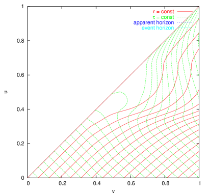
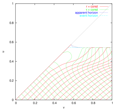
Figure 5: Penrose diagram for subcritical collapse.

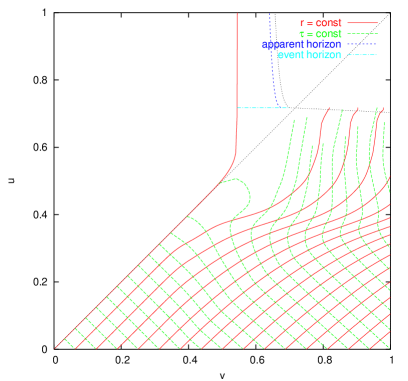
Figure 6: Penrose diagram for supercritical collapse with $M_{\text{BH}}/M_{0}\approx 0.046$.

Figure 7: Re-gauged supercritical collapse of Fig. 7. The re-gauging was done at the postprocessing stage from the same simulation run. One sees the clear similarity with the subcritical collapse shown in Fig. 7.

When we examine the Penrose diagram of a supercritical collapse as shown in Fig. 7, we see the formation of a horizon near $u\approx 0.55$. The code evolves well inside the event horizon, and we can identify the apparent horizon in the interior of the black hole. The lines of constant $r$ become spacelike beyond the apparent horizon. All the larger radii outside the black hole pile up at the horizon in this diagram.

We can pose the question if the spacetime described by Fig. 7 could possibly be the same as Fig. 7. Our original gauge choice from equation (6) fixes the $r=0$ line to coincide with $u=v$. It does not have to be this way; the null coordinates leave the possibility for a global gauge change $u\mapsto U(u)$. One can try to “un-pile” the lines of constant $r$ observers for the supercritical collapse spacetime in Fig. 7 by defining a gauge change $U(u)$ such that the second $r$ curve coincides with that in a subcritical collapse spacetime of Fig. 7. The result is shown in Fig. 7.

This stretching is rather sudden and throws the $r=0$ line into an almost null direction, but all the other finite $r$’s appear to coincide. This is non-trivial, since the residual gauge freedom is a single function of one variable, which we used to fix one value $r$. If the spacetimes are equivalent, the other $r$ and $t$ should fall into place, and similarly if the spacetimes are different they should diverge. We indeed see that the proper time and outer radii move into place, as would be expected in a convergent spacetime. It is also clear that the $r=0$ line is not convergent, and the limiting spacetime experiences infinite curvature at that one point. To address the future of this singular event, we can look at the spacetime of the limiting sequence of super- and subcritical collapses.

We now discuss the global structure of the critical spacetime. Our first question is the nature of the $r=0$ line in the course of the singular collapse event. An observer moving at some finite radius $r$ sees the collapse of a scalar field to a point, and a rebound. This is true for both the supercritical and subcritical collapse, since even when a black hole forms, the majority of the initial scalar field energy escapes, and the black hole only contains an ever smaller fraction of the initial mass as the parameter is tuned to criticality. Long after the field rebounds, the observer can measure the gravitational redshift to adjacent interior radii, and concludes that there is no redshift for most radii. In the supercritical scenario, there are significant redshifts at scales $r\lesssim M_{\text{BH}}$. But for any fixed radius observer, as one takes the limit of $p\rightarrow p^{*}$, the sphere of influence of the ever diminishing black hole mass shrinks to zero, and the spacetime converges pointwise to Minkowski at $r>0$. The convergence is not uniform, since for any given redshift difference $\epsilon$ between the observer and a fiducial interior radius, one can construct a radius $r\sim M/\epsilon$ inside which the redshift is larger than $\epsilon$. In the two limits $p\rightarrow p^{*}_{+}$ and $p\rightarrow p^{*}_{-}$, the spacetimes converge pointwise everywhere except for the line $r=0$.

A simple analogy is a singular weak field star. Consider a sequence of spacetimes with a single star of mass $M_{*}$ and radius $r_{*}=M_{*}/\epsilon$. The Newtonian potential outside the star is $V(r)=-M_{*}/r$ for $r>M_{*}/\epsilon$. To simplify the argument, we make the potential continuous and constant interior to its radius $V(r)=\epsilon$. For small values of $\epsilon$, the spacetime is in the weak field regime everywhere to order $\epsilon$. If we take a sequence of such space times with fixed $\epsilon$ and decreasing $M_{*}$, the maximal curvature $R\propto\epsilon^{3}/M_{*}^{2}$ increases without bound. There appears to be an illusory naked singularity in that limit. We can ask what the limiting spacetime looks like as $M_{*}\rightarrow 0$. The obvious answer would be empty Minkowski space. The convergence to this space is pointwise, but not uniform. In the limit, $V_{0}(r)=\lim_{M_{*}\rightarrow 0}M_{*}/r$. $V_{0}(r)$ converges to 0 pointwise, but not uniformly, so in the limit, $V_{0}(r)=0$ everywhere except for $r=0$, and it is undefined at that point. This is a removable singularity since we can define $V_{0}(0)\equiv\lim_{r\rightarrow 0}V_{0}(r)=0$, which is a unique and physically acceptable solution. We suggest that the future of the singular collapse is likewise regular everywhere, with a removable singularity at $r=0$ in the future of the collapse event.

The apparent paradox in the Penrose diagram seen in Fig. 1 arises from the gauge choice at $r=0$. This one line is poorly defined in the limit, since it becomes singular. The left panel describes the physical spacetime in the critical collapse limit, and the right one is related by a singular gauge change.

Our analysis takes a very different approach from Martin-Garcia and Gundlach Martin-Garcia:2003gz . These authors solve an elliptic equation satisfying an ansatz of discretely self-similar critical collapse. We took a limit of a series of hyperbolic initial value problems. Those authors found a possibility of specifying new Cauchy data in the elliptic solution, which is never an option for our evolutionary approach. The qualitative solution for their unique regular extension looks similar to our critical spacetime.

VI Conclusions

We have implemented a characteristic code in double-null coordinates and used it to study the global spacetime structure of a critical collapse of a scalar field. We reproduce the standard critical behavior and universal scaling. We compare the limiting spacetime from the subcritical and the supercritical collapse limits. These two limits appear qualitatively different. Based on the numerical simulations, we conjecture that the two limits converge pointwise to the same spacetime, but not uniformly. In particular, the $r=0$ line is not convergent, but all other points appear to converge pointwise. The two apparently different solutions then only differ by a gauge change. The apparent naked singularity in the upper limit obtained by the sequence of spacetimes with ever decreasing black hole mass becomes a removable singularity in the limit.

We conclude that the nature of the limiting critical collapse space time requires a careful definition of the order in which limits are taken, since the convergence is not uniform. For any collapse parameter $p$ within the critical value $|p-p^{*}|=\delta>0$, one can find sufficiently small radii within which the supercritical and subcritical solutions differ. Conversely, for any fixed $r>0$, one can find a value $\delta(r)$ where the super and sub critical space times agree to some tolerance $\epsilon$ at radius $r$. There is a unique limit, with no new Cauchy data that emits from the singular event.

References

- (1) M. W. Choptuik, Universality and scaling in gravitational collapse of a massless scalar field, Phys. Rev. Lett. 70, 9 (1993).
- (2) C. Gundlach, Critical phenomena in gravitational collapse, Phys. Rept. 376, 339 (2003) [gr-qc/0210101].
- (3) W. Israel, The formation of black holes in nonspherical collapse and cosmic censorship, Canadian Journal of Physics 64, 120 (1986).
- (4) L. M. Burko, The singularity in supercritical collapse of a spherical scalar field, Phys. Rev. D 58, 084013 (1998) [gr-qc/9803059].
- (5) J. M. Martin-Garcia and C. Gundlach, Global structure of Choptuik’s critical solution in scalar field collapse, Phys. Rev. D 68, 024011 (2003) [gr-qc/0304070].
- (6) D. Garfinkle, Choptuik scaling in null coordinates, Phys. Rev. D 51, 5558 (1995) [gr-qc/9412008].
- (7) C. Gundlach and J. Pullin, Instability of free evolution in double null coordinates, Class. Quant. Grav. 14, 991 (1997) [gr-qc/9606022].
- (8) S. Hod and T. Piran, Fine-structure of Choptuik’s mass-scaling relation, Phys. Rev. D 55, 440 (1997) [gr-qc/9606087].