The initial value problem as it relates to numerical relativity

Abstract

Spacetime is foliated by spatial hypersurfaces in the 3+1 split of General Relativity. The initial value problem then consists of specifying initial data for all fields on one such a spatial hypersurface, such that the subsequent evolution forward in time is fully determined. On each hypersurface the 3-metric and extrinsic curvature describe the geometry. Together with matter fields such as fluid velocity, energy density and rest mass density, the 3-metric and extrinsic curvature then constitute the initial data. There is a lot of freedom in choosing such initial data. This freedom corresponds to the physical state of the system at the initial time. At the same time the initial data have to satisfy the Hamiltonian and momentum constraint equations of General Relativity and can thus not be chosen completely freely. We discuss the conformal transverse traceless and conformal thin sandwich decompositions that are commonly used in the construction of constraint satisfying initial data. These decompositions allow us to specify certain free data that describe the physical nature of the system. The remaining metric fields are then determined by solving elliptic equations derived from the constraint equations. We describe initial data for single black holes and single neutron stars, and how we can use conformal decompositions to construct initial data for binaries made up of black holes or neutron stars. Orbiting binaries will emit gravitational radiation and thus lose energy. Since the emitted radiation tends to circularize the orbits over time, one can thus expect that the objects in a typical binary move on almost circular orbits with slowly shrinking radii. This leads us to the concept of quasi-equilibrium which essentially assumes that time derivatives are negligible in corotating coordinates, for binaries on almost circular orbits. We review how quasi-equilibrium assumptions can be used to make physically well motivated approximations that simplify the elliptic equations we have to solve.

Keywords: numerical relativity, compact binaries, black holes, neutron stars, gravitational waves, initial data

1 Introduction

After the first direct detection of a gravitational wave signal emitted by a binary black holes system [1, 2], the problem of faithfully simulating the evolution of binary systems of compact objects has become increasingly important. The detectors (LIGO [3, 4], VIRGO [5, 6], GEO600 [7]) use laser interferometry to measure the strains associated with passing gravitational waves [8], and offer much higher sensitivity than previous experiments aimed at direct detection of these waves. Additional detectors such as KAGRA [9] or the space borne eLISA/NGO [10] and DECIGO [11] are in planning and construction stages. In all these detectors, the measured strains are tiny and contaminated by noise. For detection and especially parameter estimation, it is thus necessary to compare the observed signals to theoretical gravitational wave templates that describe different systems.

One of the most promising sources for gravitational wave detectors is the inspiral and merger of compact objects such as black holes or neutron stars. Due to the emission of gravitational waves, the binary loses energy and the orbit tightens until finally the two objects merge. As long as the two compact objects are far apart, post-Newtonian calculations [12] can give highly accurate approximations for the orbital motion and the gravitational waves emitted by the binary. When the two objects get closer, the post-Newtonian expansion becomes more and more inaccurate and eventually breaks down. Thus the full non-linear equations of General Relativity have to be solved and computer simulations are used to obtain numerical answers [13]. From each of these computer simulations we can then extract a gravitational wave template for the simulated system. In order to start such numerical simulations we need to specify initial data that describe the initial state of the binary system. These initial data should be chosen as accurately and as realistically as possible. Otherwise the subsequent numerical evolution may not simulate the kind of system the detectors observe.

In this paper we will concentrate on how one can construct reliable initial data. In Sec. 2 we describe the basic equations that are used in numerical relativity. This is followed in Sec. 3 by a discussion of several conformal decompositions that are used to derive the equations commonly used in the construction of initial data. Sections 4 and 5 describe various methods to construct initial data for single and binary black holes, and Sec. 6 presents possible improvements. We proceed in Sec. 7 by introducing equations that are needed to describe neutron star matter. In Secs. 8 and 9 we discuss single and binary neutron star data, while Sec. 10 deals with mixed binaries. Section 11 provides a short overview of the most common computer codes that are used to compute initial data. We provide some conclusions in Sec. 12. Throughout we will use geometric units where $G=c=1$.

2 Numerical relativity

In this section we introduce the basic equations of numerical relativity. We start by discussing some equations of General Relativity and explain how they are reformulated for use in numerical simulations.

2.1 General Relativity

We recall here some of the basic equations of General Relativity with the purpose of illustrating our notation.

In Relativity theory 3-dimensional space and time are unified into 4-dimensional spacetime. In the simplest case of a flat spacetime distances in this 4-dimensional spacetime are measured as

$$ds^{2}=(dx^{1})^{2}+(dx^{2})^{2}+(dx^{3})^{2}-(dx^{0})^{2},$$ (1)

where $x^{1}$, $x^{2}$, $x^{3}$ are the usual Cartesian coordinates of Euclidean space, and $x^{0}$ is time. Usually this distance is written as

$$ds^{2}=g_{\mu\nu}dx^{\mu}dx^{\nu},$$ (2)

where the indices $\mu$ and $\nu$ run from 0 to 3, and we use the Einstein summation convention and sum over repeated indices. Here $g_{\mu\nu}$ are the components of a symmetric tensor called the spacetime metric or 4-metric. For flat spacetime in Cartesian coordinates we have $g_{\mu\nu}=\mbox{diag}(-1,1,1,1)$, but if we change coordinates $g_{\mu\nu}$ will have different values. The inverse of the 4-metric will be denoted as $g^{\mu\nu}$. Throughout we will use Greek letters to denote 4-dimensional indices that run from 0 to 3. Later when we refer to the spatial components of tensors we will use letters from the middle of the Latin alphabet. An example is the spatial 3-metric $\gamma_{ij}=\mbox{diag}(1,1,1)$ of flat space, where both $i$ and $j$ run from 1 to 3.

We denote the 4-dimensional covariant derivative operator by $\nabla_{\alpha}$. It is defined by

$$\nabla_{\alpha}g_{\mu\nu}=0$$ (3)

in order to be compatible with the 4-metric. The covariant derivative of any tensor can be given in terms of partial derivatives and the Christoffel symbols

$$\Gamma^{\alpha}_{\mu\nu}=\frac{1}{2}g^{\alpha\rho}(\partial_{\nu}g_{\rho\mu}+\partial_{\mu}g_{\rho\nu}-\partial_{\rho}g_{\mu\nu}).$$ (4)

For example, the covariant derivative of a 4-vector $V^{\mu}$ can be computed from

$$\nabla_{\alpha}V^{\mu}=\partial_{\alpha}V^{\mu}+\Gamma^{\mu}_{\alpha\nu}V^{\nu}.$$ (5)

If matter or energy is present, spacetime will become curved and the 4-metric has to be determined from the Einstein equations

$$^{4}R_{\mu\nu}-\frac{1}{2}g_{\mu\nu}{}^{4}R=8\pi T_{\mu\nu}.$$ (6)

Here $T_{\mu\nu}$ is the stress-energy tensor of matter. The Ricci tensor ${}^{4}R_{\mu\nu}={}^{4}R_{\mu\rho\nu}^{\ \ \ \ \rho}$ and the Ricci Scalar ${}^{4}R={}^{4}R_{\mu\nu}g^{\mu\nu}$ are both related to the Riemann tensor ${}^{4}R^{\mu}_{\ \nu\alpha\beta}$, defined by [14]

$${}^{4}R_{\alpha\beta\mu}^{\ \ \ \ \nu}\omega_{\nu}:=(\nabla_{\alpha}\nabla_{\beta}-\nabla_{\beta}\nabla_{\alpha})\omega_{\mu},$$ (7)

where $\omega_{\mu}$ is any one-form. Indices on all tensors can be raised and lowered with the spacetime metric $g_{\mu\nu}$. We will follow the sign conventions of Misner, Thorne and Wheeler [15], so that the Riemann tensor when computed from the Christoffel symbols in Eq. (4) is given by

$$^{4}R^{\mu}_{\ \nu\alpha\beta}=\partial_{\alpha}\Gamma^{\mu}_{\nu\beta}-\partial_{\beta}\Gamma^{\mu}_{\nu\alpha}+\Gamma^{\mu}_{\rho\alpha}\Gamma^{\rho}_{\nu\beta}-\Gamma^{\mu}_{\rho\beta}\Gamma^{\rho}_{\nu\alpha}.$$ (8)

As we have seen any tensor of any rank can be written using the index notation introduced above. However, sometimes it can be advantageous to use index free notation. We use $\vec{u}$ to denote a 4-vector $u^{\mu}$ and $\undertilde{\omega}$ to denote a one-form $\omega_{\mu}$. The contraction of the two is then written as $\vec{u}\cdot\undertilde{\omega}=u^{\mu}\omega_{\mu}$.

2.2 The 3+1 split of spacetime

Since both the 4-metric and the Ricci tensor are symmetric, it is clear that the Einstein equations in (6) are ten independent equations for the ten independent components of the 4-metric. From Eq. (8) we see that these ten equations are linear in the second derivatives and quadratic in the first derivatives of the 4-metric. However, only six of these ten equations contain second time derivatives. These six second order in time equations represent evolution equations. The other four are not evolution equations, but rather represent constraints that the 4-metric has to satisfy.

If we can solve the Einstein equations in (6) we obtain the 4-metric everywhere in space and time. While a solution for all of spacetime is certainly very useful, in practice it is possible to find such direct solutions of Eq. (6) only in rare cases where one assumes symmetries such as time independence and axisymmetry. In addition, in many astrophysical problems of interest it may not be necessary to find a solution for all of time. One usually would like to start from some given initial conditions at some initial time and then to calculate the state of the system at some later time. For example, for a particle in classical mechanics one starts by giving the initial position and velocity, and then calculates position and velocity at a later time. We would like to do the same for General Relativity and specify initial data (i.e. some fields and their time derivatives) at some initial time and then calculate these fields at a later time. In order to do this we use the 3+1 split of spacetime [16]: We foliate spacetime by spacelike 3-dimensional hypersurfaces or slices, i.e. surfaces with a normal vector $n^{\mu}$ that is timelike. As time coordinate $x^{0}$ we use a function $t$ which is constant on each hypersurface, but increases as we go from one hypersurface to the next. We then define the lapse by

$$\alpha:=\sqrt{\frac{-1}{g^{\mu\nu}\partial_{\mu}t\partial_{\nu}t}}=\sqrt{\frac{-1}{g^{00}}}.$$ (9)

The normal vector thus must satisfy

$$n_{\mu}=-\alpha\partial_{\mu}t=(-\alpha,0,0,0)$$ (10)

in order for it to be normalized such that

$$g^{\mu\nu}n_{\mu}n_{\nu}=-1.$$ (11)

The minus sign in Eq. (10) is chosen such that $n^{\mu}$ points in the future direction of increasing $t$. Notice that while $n^{\mu}$ is orthogonal to each hypersurface, $n^{\mu}$ is not in general tangent to lines of constant spatial coordinates $x^{i}=const$, since we are still free to choose arbitrary spatial coordinates on each hypersurface. Indeed the tangent vector $t^{\mu}$ to lines of constant spatial coordinates is given by

$$t^{\mu}=(\partial_{t})^{\mu}=(1,0,0,0),$$ (12)

where we have normalized $t^{\mu}$ such that

$$t^{\mu}\partial_{\mu}t=1.$$ (13)

The latter also implies

$$t^{\mu}n_{\mu}=-\alpha$$ (14)

from which it follows that

$$t^{\mu}=\alpha n^{\mu}+\beta^{\mu},$$ (15)

where $\beta^{\mu}$ is an arbitrary spatial vector, i.e. any vector that satisfies $\beta^{\mu}n_{\mu}=0$. Once the foliation is given the lapse $\alpha$ and the normal vector $n^{\mu}$ are fixed. Yet the direction of the vector $t^{\mu}$ still depends on the choice of spatial coordinates on each hypersurface. This freedom to choose spatial coordinates is encapsulated in the spatial vector $\beta^{\mu}=(0,\beta^{i})$, which is called the shift vector.

2.3 3-metric, spatial covariant derivative and extrinsic curvature

We now define the 3-metric as

$$\gamma_{\mu\nu}=g_{\mu\nu}+n_{\mu}n_{\nu}$$ (16)

which is the projection of the 4-metric onto the hypersurface with normal vector $n^{\mu}$. This is a proper 4-tensor whose indices can be raised and lowered with the 4-metric $g_{\mu\nu}$. Since $n_{i}=0$ we find $\gamma_{ij}=g_{ij}$ and $\gamma^{i}_{j}=g^{i}_{j}=\delta^{i}_{j}$. From Eq. (16) we also find $\gamma^{0\nu}=\gamma^{\mu\nu}n_{\mu}/(-\alpha)=0$ and thus $\gamma^{ik}\gamma_{kj}=\gamma^{i\nu}\gamma_{\nu j}=\gamma^{i\nu}g_{\nu j}=\gamma^{i}_{j}=\delta^{i}_{j}$.

From Eqs. (12) and (15) we find that

$$g_{00}=g_{\mu\nu}t^{\mu}t^{\nu}=-\alpha^{2}+g_{\mu\nu}\beta^{\mu}\beta^{\nu}=-\alpha^{2}+\gamma_{ij}\beta^{i}\beta^{j}$$ (17)

and

$$g_{0j}=g_{\mu j}t^{\mu}=-\alpha n_{j}+\beta_{j}=\beta_{j}$$ (18)

where $\beta_{j}=g_{\mu j}\beta^{\mu}=\gamma_{ij}\beta^{i}$. Using the latter two equations, the line element in Eq. (2) can now be written as

$$ds^{2}=-\alpha^{2}dt^{2}+\gamma_{ij}(dx^{i}+\beta^{i}dt)(dx^{j}+\beta^{j}dt).$$ (19)

The 3-metric defined in Eq. (16) can be used to project any tensor $T^{\alpha_{1}\alpha_{2}...}_{\ \ \ \ \ \beta_{1}\beta_{2}...}$ onto the spatial hypersurface. The resulting tensor $S^{\alpha_{1}\alpha_{2}...}_{\ \ \ \ \ \beta_{1}\beta_{2}...}=\gamma^{\alpha_{1}}_{\gamma_{1}}\gamma^{\alpha_{2}}_{\gamma_{2}}...\gamma_{\beta_{1}}^{\delta_{1}}\gamma_{\beta_{2}}^{\delta_{2}}...T^{\gamma_{1}\gamma_{2}...}_{\ \ \ \ \ \delta_{1}\delta_{2}...}$ is called a spatial tensor since it is orthogonal to $n_{\alpha}$ in each index. Note that the indices on any spatial tensor can be raised or lowered by using either the 3-metric $\gamma_{ij}$ or the 4-metric $g_{\mu\nu}$. The result will be the same since $\gamma_{\mu\nu}n^{\nu}=0$.

We define the spatial covariant derivative of any spatial tensor $S^{\alpha_{1}\alpha_{2}...}_{\ \ \ \ \ \beta_{1}\beta_{2}...}$ as

$$D_{\mu}S^{\alpha_{1}\alpha_{2}...}_{\ \ \ \ \ \beta_{1}\beta_{2}...}:=\gamma_{\mu}^{\rho}\gamma^{\alpha_{1}}_{\gamma_{1}}\gamma^{\alpha_{2}}_{\gamma_{2}}...\gamma_{\beta_{1}}^{\delta_{1}}\gamma_{\beta_{2}}^{\delta_{2}}...\nabla_{\rho}S^{\gamma_{1}\gamma_{2}...}_{\ \ \ \ \ \delta_{1}\delta_{2}...},$$ (20)

where we have projected all free indices onto the spatial hypersurface. From Eq. (16) it immediately follows that

$$D_{\mu}\gamma_{\alpha\beta}=0,$$ (21)

so that the spatial covariant derivative operator $D_{\mu}$ is compatible with the 3-metric $\gamma_{\alpha\beta}$. This also implies that the spatial covariant derivative $D_{i}S^{k_{1}k_{2}...}_{\ \ \ \ \ l_{1}l_{2}...}$ of any spatial tensor $S^{k_{1}k_{2}...}_{\ \ \ \ \ l_{1}l_{2}...}$ can be computed with the help of 3-dimensional Christoffel symbols, which can be computed from the 3-metric $\gamma_{ij}$.

In order to describe the curvature of a $t=const$ hypersurface one introduces the extrinsic curvature

$$K_{\mu\nu}:=-\gamma^{\alpha}_{\mu}\gamma^{\beta}_{\nu}\nabla_{\alpha}n_{\beta}.$$ (22)

It can be shown that $K_{\mu\nu}$ is symmetric and also given by

$$K_{\mu\nu}=-\frac{1}{2}\pounds_{n}\gamma_{\mu\nu},$$ (23)

where $\pounds_{n}$ is the Lie derivative (see A) along the vector $n^{\mu}$. We can thus express $K_{ij}$ also as (see A.4)

$$K_{ij}=-\frac{1}{2\alpha}(\partial_{t}\gamma_{ij}-D_{i}\beta_{j}-D_{j}\beta_{i}),$$ (24)

which tells us how time derivatives of the 3-metric are related to the extrinsic curvature. From its definition in Eq. (22) it is clear that the extrinsic curvature tells us how the normal vector $n^{\mu}$ changes across a $t=const$ hypersurface. It thus measures how this hypersurface is curved with respect to the 4-dimensional space it is embedded in. However, the 3-dimensional space within each hypersurface can be curved as well. This so called intrinsic curvature is described by the 3-dimensional Riemann tensor $R^{i}_{\ jkl}$ that can be computed from the 3-metric $\gamma_{ij}$ and its resulting 3-dimensional Christoffel symbols using Eqs. (4) and (8) for $\gamma_{ij}$ instead of $g_{\mu\nu}$. We will see below how the curvature of spacetime described by the 4-dimensional Riemann tensor ${}^{4}R^{\mu}_{\ \nu\alpha\beta}$ is related to the extrinsic curvature $K_{ij}$ and the intrinsic curvature $R^{i}_{\ jkl}$. Also notice that in three dimensions, the Riemann tensor has the same number of independent components and carries the same information as the 3-dimensional Ricci tensor $R_{jl}=R^{i}_{\ jil}$.

2.4 Einstein’s equations and the 3+1 split

Going back to our example of a particle in classical mechanics, we see that the 3-metric $\gamma_{ij}$ is analogous to the particle position, while the extrinsic curvature $K_{ij}$ is analogous to its velocity. Of course, in order to compute the time evolution of a particle we also need the equation of motion that tells us the time derivative of the velocity. In our case we will use Einsteins equations to find additional equations that tell us how $K_{ij}$ evolves in time. This is done by relating the 4-dimensional Riemann tensor ${}^{4}R_{\alpha\beta\mu\nu}$ to the 3-dimensional Riemann tensor $R_{\alpha\beta\mu\nu}$ with the help of the Gauss-Codazzi and Codazzi-Mainardi relations given by (see e.g. [17] or [18])

$$R_{\alpha\beta\mu\nu}+K_{\alpha\mu}K_{\beta\nu}-K_{\alpha\nu}K_{\beta\mu}=\gamma_{\alpha}^{\alpha^{\prime}}\gamma_{\beta}^{\beta^{\prime}}\gamma_{\mu}^{\mu^{\prime}}\gamma_{\nu}^{\nu^{\prime}}{}^{4}R_{\alpha^{\prime}\beta^{\prime}\mu^{\prime}\nu^{\prime}}$$ (25)

and

$$D_{\beta}K_{\alpha\mu}-D_{\alpha}K_{\beta\mu}=\gamma_{\alpha}^{\alpha^{\prime}}\gamma_{\beta}^{\beta^{\prime}}\gamma_{\mu}^{\mu^{\prime}}{}^{4}R_{\alpha^{\prime}\beta^{\prime}\mu^{\prime}\nu}n^{\nu}.$$ (26)

One can also show that

$$\nabla_{\mu}n_{\nu}=-K_{\mu\nu}-n_{\mu}(\nabla_{\nu}+n_{\nu}n^{\rho}\nabla_{\rho})\ln\alpha=-K_{\mu\nu}-n_{\mu}D_{\nu}\ln\alpha.$$ (27)

By looking at the different projections of the Einstein equations (6) onto $n^{\mu}$ and $\gamma^{\mu\nu}$ and using Eqs. (25), (26), (27) and (7) we find that Einstein’s equations split into the evolution equations

$$\partial_{t}\gamma_{ij} = -2\alpha K_{ij}+\pounds_{\beta}\gamma_{ij}$$ (28)

$$\partial_{t}K_{ij} = \alpha(R_{ij}-2K_{il}K^{l}_{j}+KK_{ij})-D_{i}D_{j}\alpha+\pounds_{\beta}K_{ij}$$ (29)

$$-8\pi\alpha S_{ij}+4\pi\alpha\gamma_{ij}(S-\rho)$$

and the so called Hamiltonian and momentum constraint equations

$$R-K_{ij}K^{ij}+K^{2} = 16\pi\rho$$ (30)

$$D_{j}(K^{ij}-\gamma^{ij}K) = 8\pi j^{i}.$$ (31)

Here $R_{ij}$ and $R$ are the Ricci tensor and scalar computed from $\gamma_{ij}$, $D_{i}$ is the derivative operator compatible with $\gamma_{ij}$ and all indices here are raised and lowered with the 3-metric $\gamma_{ij}$. The source terms $\rho$, $j^{i}$, $S_{ij}$ and $S=\gamma^{ij}S_{ij}$ are projections of the stress-energy tensor $T_{\mu\nu}$ given by

$$\rho = T_{\mu\nu}n^{\mu}n^{\nu}$$

$$j^{i} = -T_{\mu\nu}n^{\mu}\gamma^{\nu i}$$

$$S^{ij} = T_{\mu\nu}\gamma^{\mu i}\gamma^{\nu j}$$ (32)

and correspond to the energy density, flux and stress-tensor seen by an observer moving with 4-velocity $n^{\mu}$.

2.5 Constraints, gauge freedom and physical degrees of freedom

The evolution equations in Eqs. (28) and (29) tell us how we can obtain $\gamma_{ij}$ and $K_{ij}$ at any time, if we are given $\gamma_{ij}$ and $K_{ij}$ at some initial time. As one can see, the constraint equations (30) and (31) do not contain any time derivatives and thus are equations that need to be satisfied on each spatial hypersurface. Thus when we construct initial data, we have to ensure that both $\gamma_{ij}$ and $K_{ij}$ satisfy the constraint equations at the initial time. It can then be shown that the evolution equations will preserve the constraints. For this reason constructing initial data is a non-trivial task in the sense that we cannot freely choose the 12 fields $\gamma_{ij}$ and $K_{ij}$. Rather these fields are subject to the 4 constraints in Eqs. (30) and (31). This leaves us with only 8 freely specifiable fields. However, in General Relativity we are free to choose any coordinates we like. Since there are 4 coordinates that we can freely choose, the 8 freely specifiable fields in $\gamma_{ij}$ and $K_{ij}$ can really contain only 4 physical fields that are independent of our coordinate choice. Since we specify both $\gamma_{ij}$ and its time derivative $K_{ij}$ (see Eq. (24)) 2 of these 4 fields are merely time derivatives of the other 2 fields. Thus we are dealing with only 2 physical degrees of freedom, as expected for gravity.

The freedom to choose coordinates is usually referred to as gauge freedom and connected to the choice of lapse $\alpha$ shift $\beta^{i}$. If we only change the 3 spatial coordinates, all components of $\gamma_{ij}$ and $K_{ij}$ as well as the shift will change in general, but the spatial hypersurfaces themselves are unchanged, so that the normal vector $n^{\mu}$ and the lapse $\alpha$ will not change. If we change the time coordinate $t$, the hypersurfaces themselves will also change so that now $n^{\mu}$ and the lapse $\alpha$ will change as well [19].

3 Conformal decompositions and initial data construction

As already mentioned, the initial data $\gamma_{ij}$ and $K_{ij}$ cannot be freely chosen, since they must satisfy the constraint equations (30) and (31). However, since the constraint equations alone cannot determine the initial data either, Eqs. (30) and (31) do not have unique solutions and are thus not directly useful in constructing initial data. For this reason so called conformal decompositions have been developed. Using these decompositions it is possible to start by specifying arbitrary $\gamma_{ij}$ and $K_{ij}$ that may not satisfy the constraints. In a second step these $\gamma_{ij}$ and $K_{ij}$ are then modified in such a way that they satisfy the constraints. This second step involves solving certain elliptic equations for 4 auxiliary quantities that are used to compute the final constraint satisfying $\gamma_{ij}$ and $K_{ij}$. These elliptic equations have the great advantage that they generally have unique solutions once appropriate boundary conditions are specified (see B). Except for simple cases with many symmetries these elliptic equations are usually solved numerically [20].

Following Lichnerowicz [21] and York [22, 23] we start by decomposing the 3-metric $\gamma_{ij}$ into a conformal factor $\psi$ and a conformal metric $\bar{\gamma}_{ij}$ such that

$$\gamma_{ij}=\psi^{4}\bar{\gamma}_{ij}.$$ (33)

Using this decomposition the Ricci scalar can be written as

$$R=\psi^{-4}\bar{R}-8\psi^{-5}\bar{D}_{k}\bar{D}^{k}\psi.$$ (34)

Here $\bar{D}_{k}$ is the derivative operator compatible with the conformal metric $\bar{\gamma}_{ij}$ and $\bar{R}$ the Ricci scalar computed from $\bar{\gamma}_{ij}$. It is also possible to verify that for any symmetric and tracefree tensor $M^{ij}$ we have [24]

$$D_{j}M^{ij}=\psi^{-10}\bar{D}_{j}\bar{M}^{ij}$$ (35)

if we define

$$\bar{M}^{ij}=\psi^{10}M^{ij}.$$ (36)

Let us also introduce a symmetric tracefree differential operator $L$. It is defined by its action on any vector $W^{i}$ by

$$(LW)^{ij}:=D^{i}W^{j}+D^{j}W^{i}-\frac{2}{3}\gamma^{ij}D_{k}W^{k}.$$ (37)

It is sometimes referred to as conformal Killing form since it is related to the Lie derivative of the tensor density $\gamma^{-1/3}\gamma_{ij}$ of weight $-2/3$, where $\gamma=\det(\gamma_{ij})$. Using Eq. (244) we find

$$\pounds_{W}(\gamma^{-1/3}\gamma_{ij})=\gamma^{-1/3}(LW)_{ij}.$$ (38)

So if $W^{i}$ is a Killing vector of the metric $\gamma^{-1/3}\gamma_{ij}$ with $\pounds_{W}(\gamma^{-1/3}\gamma_{ij})=0$, we will have $(LW)^{ij}=0$. Notice that in general $\gamma^{-1/3}\gamma_{ij}$ is not the same as the conformal metric $\bar{\gamma}_{ij}$.

One can show that

$$(LW)^{ij}=\psi^{-4}(\bar{L}W)^{ij},$$ (39)

where $(\bar{L}W)^{ij}:=\bar{D}^{i}W^{j}+\bar{D}^{j}W^{i}-\frac{2}{3}\bar{\gamma}^{ij}\bar{D}_{k}W^{k}$ is computed using the conformal metric.

Next, the extrinsic curvature is split into its trace $K=\gamma_{ij}K^{ij}$ and its tracefree part $A^{ij}$ by writing it as

$$K^{ij}=A^{ij}+\frac{1}{3}\gamma^{ij}K.$$ (40)

The tracefree part is rescaled as

$$A^{ij}=\psi^{-10}\bar{A}^{ij}.$$ (41)

Note that the factor of $\psi^{-10}$ in Eq. (41) has been picked so that Eq. (35) applies to $A^{ij}$.

Inserting Eqs. (34), (40) and (41) into the Hamiltonian constraint (30) yields

$$8\bar{D}_{k}\bar{D}^{k}\psi-\bar{R}\psi+\psi^{-7}\bar{A}^{ij}\bar{A}_{ij}-\frac{2}{3}\psi^{5}K=-16\pi\psi^{5}\rho,$$ (42)

where indices on the barred quantities are raised and lowered with $\bar{\gamma}_{ij}$. We will use this equation for the Hamiltonian constraint to compute the conformal factor in the different conformal decompositions discussed below. Note, however, that these decompositions differ in how $\bar{A}^{ij}$ is split further.

3.1 The conformal transverse traceless decomposition

We consider first the conformal transverse traceless (CTT) decomposition, where we split [25]

$$\bar{A}^{ij}=\bar{M}^{ij}+\frac{1}{\bar{\sigma}}(\bar{L}W)^{ij}$$ (43)

in two pieces. Here $\bar{M}^{ij}$ is tracefree but otherwise arbitrary and $\bar{\sigma}$ is some positive weighting factor that we can choose. The vector $W^{i}$ will be computed below.

The Hamiltonian constraint is written as in Eq. (42) with $\bar{A}^{ij}$ defined as in Eq. (43). When we insert Eqs. (40), (41) and (43) into the momentum constraint (31) we find

$$\bar{D}_{j}\left[\frac{1}{\bar{\sigma}}(\bar{L}W)^{ij}\right]+\bar{D}_{j}\bar{M}^{ij}-\frac{2}{3}\psi^{6}\bar{D}^{i}K=8\pi\psi^{10}j^{i}.$$ (44)

Both Eqs. (42) and (44) are elliptic equations. The weighting factor is often simply set to $\bar{\sigma}=1$. In this case we obtain the standard CTT decomposition often called the York-Lichnerowicz decomposition [21, 22, 23]. However, other choices are possible. For example, for $\bar{\sigma}=\psi^{-6}$ we obtain the so called physical CTT decomposition [20].

Let us now discuss how Eqs. (42) and (44) are used in practice. We start with some reasonable guess or approximation for the physical situation we want to describe. For example, if we want to find initial data for two black holes we could simply take the superposition of the 3-metrics and extrinsic curvatures for two single black hole solutions . Since the superposition principle does not hold in a non-linear theory like General Relativity, this superposition will at best be an approximate solution that we denote here by $\gamma_{ij}^{approx}$ and $K^{ij}_{approx}$. Hence $\gamma_{ij}^{approx}$ and $K^{ij}_{approx}$ will not satisfy the Hamiltonian and momentum constraints. However, using the above CTT decomposition we can now construct a $\gamma_{ij}$ and $K^{ij}$ that will satisfy the constraints if we set

$$\bar{\gamma}_{ij} = \gamma_{ij}^{approx},$$

$$K = K_{approx}=\gamma_{ij}^{approx}K^{ij}_{approx},$$

$$\bar{M}^{ij} = K^{ij}_{approx}-\frac{1}{3}\gamma^{ij}_{approx}K_{approx},$$ (45)

and then solve Eqs. (42) and (44) for $\psi$ and $W^{i}$. Once we have these solutions we can use Eq. (33) and Eqs. (40), (41) and (43) to obtain a $\gamma_{ij}$ and $K^{ij}$ that are now guaranteed to satisfy the Hamiltonian and momentum constraints.

3.2 The conformal thin sandwich approach

A form of the conformal thin sandwich formalism (called the Wilson-Mathews approach [26, 27]) was first introduced under the assumption that the conformal metric is flat, i.e. $\bar{\gamma}_{ij}=\delta_{ij}$. Here we relax this assumption and present the more general conformal thin sandwich (CTS) decomposition proposed by York [28]. Like the CTT decomposition, it starts again with the conformal metric decomposition in Eq. (33). However, in order to have a direct handle on time derivatives one also introduces

$$\bar{u}_{ij}:=\partial_{t}\bar{\gamma}_{ij}$$ (46)

and demands that

$$\partial_{t}\bar{\gamma}=0,$$ (47)

i.e. that the time evolution of conformal factor be chosen such that the determinant of the conformal metric $\bar{\gamma}$ is instantaneously constant. The latter condition yields

$$\bar{u}_{ij}=\psi^{-4}(\partial_{t}\gamma_{ij}-\frac{1}{3}\gamma_{ij}\partial_{t}\ln\gamma),$$ (48)

where $\gamma=\det(\gamma_{ij})$. Together with $\partial_{t}\ln\gamma=\gamma^{ij}\partial_{t}\gamma_{ij}$, Eqs. (24) and (40) we obtain

$$\bar{u}_{ij}=\psi^{-4}(-2\alpha A_{ij}+(L\beta)_{ij}).$$ (49)

Using Eq. (39) for $W^{i}=\beta^{i}$, Eq. (49) can be rewritten as

$$\bar{A}^{ij}=\frac{1}{2\bar{\alpha}}\left[(\bar{L}\beta)^{ij}-\bar{u}^{ij}\right],$$ (50)

where we have defined

$$\bar{\alpha}=\psi^{-6}\alpha.$$ (51)

Inserting Eqs. (34), (40) and (50) into the Hamiltonian constraint (30) yields again Eq. (42), but this time with $\bar{A}^{ij}$ defined according Eq. (50). When we insert Eqs. (40) and (50) into the momentum constraint (31) we find

$$\bar{D}_{j}\left[\frac{1}{2\bar{\alpha}}\left\{(\bar{L}\beta)^{ij}-\bar{u}^{ij}\right\}\right]-\frac{2}{3}\psi^{6}\bar{D}^{i}K=8\pi\psi^{10}j^{i}.$$ (52)

From Eqs. (50) and (52) we can see that the CTS equations can be obtained from the CTT equations by setting

$$\bar{\sigma} = 2\bar{\alpha},$$

$$W^{i} = \beta^{i},$$

$$\bar{M}^{ij} = -\frac{\bar{u}^{ij}}{2\bar{\alpha}}.$$ (53)

Up to this point the CTS approach may not seem to differ very much from the conformal transverse traceless approach. Once we specify $\bar{\gamma}_{ij}$, $\bar{u}^{ij}$, $K$ and $\bar{\alpha}$, we can solve Eqs. (42) and (52) for $\psi$ and $\beta^{i}$ and then use Eq. (33) and Eqs. (40) and (50) to obtain a $\gamma_{ij}$ and $K^{ij}$ that are now guaranteed to satisfy the Hamiltonian and momentum constraints. Notice, however, that we do not just obtain initial data for the 3-metric and extrinsic curvature in this way. We also obtain a preferred lapse $\alpha=\psi^{6}\bar{\alpha}$ and shift $\beta^{i}$.

So far $\bar{\alpha}$ was an arbitrarily chosen function. It is possible to relate it to the time derivative of $K$. From Eqs. (29) and (30) we find that

$$\partial_{t}K=\beta^{i}D_{i}K-D_{i}D^{i}\alpha+\alpha\left(A^{ij}A_{ij}+\frac{1}{3}K^{2}\right)+4\pi\alpha(S+\rho).$$ (54)

Thus the lapse $\alpha$ is related to $\partial_{t}K$. Using Eqs. (51) and (42), Eq. (54) can be rewritten as an elliptic equation for $\bar{\alpha}$. We find

$$\bar{D}_{i}\bar{D}^{i}\bar{\alpha} + \bar{\alpha}\left[\frac{3}{4}\bar{R}-\frac{7}{4\psi^{8}}\bar{A}^{ij}\bar{A}_{ij}+\frac{\psi^{4}}{6}K^{2}+42(\bar{D}_{i}\ln\psi)(\bar{D}^{i}\ln\psi)\right]$$ (55)

$$+14\bar{D}_{i}\bar{\alpha}\bar{D}^{i}\ln\psi+\psi^{-2}(\partial_{t}K-\beta^{i}\bar{D}_{i}K)=4\pi\bar{\alpha}\psi^{4}(S+4\rho).$$

With the latter it is now possible to specify $\partial_{t}K$ instead of $\bar{\alpha}$. The fact that we can directly specify the time derivatives $\bar{u}^{ij}$ and $\partial_{t}K$ is usually exploited when one wants to construct initial data in quasi-equilibrium situations, where a coordinate system exists in which the time derivatives of 3-metric and extrinsic curvature either vanish or are small in some way, as we will discuss below.

Often Eq. (55) for $\bar{\alpha}$ is rewritten as an equation for $\psi\alpha$ and thus $\alpha$. Using Eqs. (51), (42) and (55) we obtain

$$\bar{D}_{i}\bar{D}^{i}(\psi\alpha) - \psi\alpha\left[\frac{1}{8}\bar{R}+\frac{5}{12}\psi^{4}K^{2}+\frac{7}{8}\psi^{-8}\bar{A}^{ij}\bar{A}_{ij}+2\pi\psi^{4}(\rho+2S)\right]$$ (56)

$$=-\psi^{5}(\partial_{t}K-\beta^{i}\bar{D}_{i}K).$$

3.3 Boundary conditions at spatial infinity

The conformal decompositions discussed above result in elliptic equations that require boundary conditions. In the case of the CTT decomposition we have to solve Eqs. (42) and (44) for $\psi$ and $W^{i}$. This is usually done in asymptotically inertial coordinates, i.e. coordinates such that the 4-metric approaches the Minkowski metric $\mbox{diag}(-1,1,1,1)$ at spatial infinity which we denote by $r\to\infty$. In this case we obtain

$$\lim_{r\to\infty}\alpha=1,\ \ \ \lim_{r\to\infty}\beta^{i}=0,\ \ \ \lim_{r\to\infty}\gamma_{ij}=\delta_{ij},\ \ \ \lim_{r\to\infty}K^{ij}=0.$$ (57)

Usually we also choose

$$\lim_{r\to\infty}\bar{\gamma}_{ij}=\delta_{ij},$$ (58)

so that Eq. (33) implies

$$\lim_{r\to\infty}\psi=1.$$ (59)

To ensure $\lim_{r\to\infty}K^{ij}=0$ we usually choose

$$\lim_{r\to\infty}\bar{M}^{ij}=0=\lim_{r\to\infty}K,$$ (60)

which together with Eqs. (40), (41) and (43) yields

$$\lim_{r\to\infty}W^{i}=0.$$ (61)

Once Eqs. (42) and (44) are supplemented by the boundary conditions (59) and (61) at infinity we will obtain unique solutions for $\psi$ and $W^{i}$.

In the case of the CTS decomposition we have to solve Eqs. (42), (52) and (55) for $\psi$, $\beta^{i}$ and $\bar{\alpha}$. If we again work in asymptotically inertial coordinates which result in Eq. (57) at spatial infinity, we find again Eq. (59), as well as

$$\lim_{r\to\infty}\bar{\alpha}=1$$ (62)

and

$$\lim_{r\to\infty}\beta^{i}=0.$$ (63)

However, sometimes it is convenient to work in a corotating frame, which is obtained by changing the spatial coordinates such that they rotate with a constant angular velocity $\Omega$ with respect to the asymptotically inertial coordinates at infinity that are used in Eq. (57). When we change coordinates to this corotating frame the 4-metric components change such that now

$$\lim_{r\to\infty}\alpha=1,\ \ \ \lim_{r\to\infty}\beta^{i}=\lim_{r\to\infty}\Omega\Phi^{i},\ \ \ \lim_{r\to\infty}\gamma_{ij}=\delta_{ij},\ \ \ \lim_{r\to\infty}K^{ij}=0.$$ (64)

Here $\Phi^{i}$ is an asymptotic rotational Killing vector at spatial infinity. Hence the boundary conditions for $\psi$ and $\bar{\alpha}$ are unchanged, while the boundary condition for the shift becomes

$$\lim_{r\to\infty}\beta^{i}=\Omega\Phi^{i}.$$ (65)

Together with these boundary conditions the elliptic equations (42), (52) and (55) have unique solutions, provided no other boundaries are present.

Notice that the shift condition (65) can be problematic for some numerical codes since $\beta_{i}\beta^{i}\to\Omega^{2}r^{2}$ as $r\to\infty$, so that the shift becomes infinite at spatial infinity. This problem is usually avoided by replacing the shift $\beta^{i}$ by

$$\beta^{i}=B^{i}+\Omega\Phi^{i}$$ (66)

in equations such as (50) and (52). These equations contain the shift only in the form $(\bar{L}\beta)^{ij}$, and since

$$(\bar{L}\Phi)^{ij}=0$$ (67)

when $\bar{\gamma}_{ij}$ is flat, Eqs. (50) and (52) still have the same form, only with $\beta^{i}$ replaced by $B^{i}$. The boundary condition for $B^{i}$ then is simply

$$\lim_{r\to\infty}B^{i}=0.$$ (68)

3.4 ADM quantities at spatial infinity and the Komar integral

The ADM mass $M^{ADM}_{\infty}$ and angular momentum $J^{ADM}_{\infty}$ at spatial infinity ($r\rightarrow\infty$) are given by

$$M^{ADM}_{\infty}=\sqrt{-P^{ADM}_{\mu\ \infty}P^{ADM}_{\nu\ \infty}\eta^{\mu\nu}},$$ (69)

$$P^{ADM}_{0\ \infty}=\frac{1}{16\pi}\int_{S_{\infty}}(\gamma_{ij,i}-\gamma_{ii,j})d{S}^{j},$$ (70)

$$P^{ADM}_{i\ \infty}=\frac{1}{8\pi}\int_{S_{\infty}}({K}_{ij}-K\eta_{ij})d{S}^{j},$$ (71)

and

$$J^{ADM}_{\infty}=\frac{1}{8\pi}\int_{S_{\infty}}({K}_{ij}\Phi^{j}-K\Phi_{i})d{S}^{i}.$$ (72)

Here $\Phi^{i}$ is again the asymptotic rotational Killing vector at spatial infinity. Note that these definitions are valid only in coordinates where the 4-metric approaches the Minkowski metric at spatial infinity. In this case lower and upper spatial indices do not need to be distinguished, so that summation is implied over any repeated spatial indices. The integrals here are over a closed sphere (denoted by $S_{\infty}$) at spatial infinity. In spherical coordinates $d{S}^{j}$ is given by $4\pi r^{2}(\sin\theta\cos\phi,\sin\theta\sin\phi,\cos\theta)d\theta d\phi$. $M^{ADM}_{\infty}$ and $J^{ADM}_{\infty}$ tell us how much mass and angular momentum is contained in the entire spacetime . In the case where $\gamma_{ij}$ in Eq. (33) is conformally flat (and if $P^{ADM}_{i\ \infty}=0$) the ADM mass simplifies to

$$M^{ADM}_{\infty}=-\frac{1}{2\pi}\int_{S_{\infty}}\partial_{j}\psi d{S}^{j}.$$ (73)

If the spacetime possess a Killing vector $\xi^{\mu}$, i.e. a vector satisfying

$$\pounds_{\xi}g_{\mu\nu}=\nabla_{(\mu}\xi_{\nu)}=0,$$ (74)

then the Komar integral [29, 30, 14]

$$I_{K}(\xi,S)=-\frac{1}{8\pi}\oint_{S}{\epsilon}_{\alpha\beta\mu\nu}\nabla^{\mu}\xi^{\nu}dx^{\alpha}\wedge dx^{\beta}$$ (75)

integrated over any closed 3-surface $S$ containing the sources yields a value that is independent of $S$.

For a time-like Killing vector that is normalized to $\xi^{\mu}\xi_{\mu}=-1$ at spatial infinity $I_{K}(\xi,S)=M^{ADM}_{\infty}$, while for an axial Killing vector that approaches the asymptotic rotational Killing vector $\Phi^{\mu}$ at spatial infinity $I_{K}(\xi,S)=-2J^{ADM}_{\infty}$ [30]. We now consider a helical Killing vector $\xi^{\mu}$ that is given by

$$\xi^{\mu}=\alpha T^{\mu}+\Omega\Phi^{\mu}$$ (76)

at spatial infinity, where $T^{\mu}$ and $\Phi^{\mu}$ are the asymptotic time-translation and rotational Killing vectors at spatial infinity and $\Omega$ is a constant. If $\xi^{a}$ is normalized such that

$$\lim_{r\rightarrow\infty}\xi^{a}n_{a}=-1,$$ (77)

then the Komar integral over a sphere at $r\rightarrow\infty$ becomes [30, 31]

$$I_{K}(\xi,S)=M^{ADM}_{\infty}-2\Omega J^{ADM}_{\infty}.$$ (78)

3.5 Quasi-equilibrium assumptions for the metric variables of binary systems

We now make some additional simplifying assumptions to better deal with quasi-equilibrium situations. For concreteness, let us discuss a binary system made up of two orbiting objects that could be stars or black holes. Such a system will radiate gravitational waves that carry away energy. Thus over time the two objects will spiral towards each other. According to post-Newtonian predictions [32, 33] the orbits circularize on a timescale which is much shorter than the inspiral timescale due to the emission of gravitational waves. The same circularization effect has also been shown in the extreme mass ratio limit in Kerr spacetime [34, 35, 36]. Hence when we set up initial data we often assume that the binary is in an approximately circular orbit. The circular orbital motion then can be transformed away by changing to a corotating coordinate system, i.e. a coordinate system that rotates with the orbital angular velocity of the binary with respect to asymptotically inertial coordinates. In this corotating system the two objects do not move, which means $\partial_{t}g_{\mu\nu}$ vanishes at least approximately. This implies that the time evolution vector $t^{\mu}$ is an approximate symmetry of the spacetime, which in turn implies the existence of an approximate helical Killing vector $\xi^{\mu}$ (see e.g. [31, 37]) with

$$\pounds_{\xi}g_{\mu\nu}\approx 0.$$ (79)

Here $\pounds_{\xi}$ is the Lie derivative (see A.3) with respect to the vector $\xi^{\mu}$. Corotating coordinates are understood as the coordinates chosen such that $t^{\mu}$ lies along $\xi^{\mu}$, such that

$$\xi^{\mu}=t^{\mu}={\alpha}n^{\mu}+\beta^{\mu}.$$ (80)

Since we are considering orbiting binaries, this Killing vector would have to be a helical Killing vector, which means that at spatial infinity ($r\rightarrow\infty$)

$$n^{\mu}=T^{\mu}\ \ \mbox{and}\ \ \beta^{\mu}=\Omega\Phi^{\mu},$$ (81)

where $T^{\mu}$ and $\Phi^{\mu}$ are the asymptotic time-translation and rotational Killing vectors at spatial infinity and $\Omega$ is the angular velocity with which the binary rotates. In asymptotically inertial coordinates we have $T^{\mu}=(1,0,0,0)$ and $\Phi^{\mu}=(0,-x^{2}+x_{CM}^{2},x^{1}-x_{CM}^{1},0)$, where we have chosen the rotational Killing vector to correspond to a rotation about the a line through the center of mass $x_{CM}^{i}$ parallel to $x^{3}$-axis.

An approximate helical Killing vector with $\pounds_{\xi}g_{\mu\nu}\approx 0$ implies that the Lie derivatives with respect to $\xi^{\mu}$ of all 3+1 quantities similarly vanish approximately. For the initial data construction using the CTS decomposition we will use

$$\pounds_{\xi}\bar{\gamma}_{ij}\approx\pounds_{\xi}K\approx 0.$$ (82)

In a corotating coordinate system where the time evolution vector $t^{\mu}$ lies along $\xi^{\mu}$, the time derivatives of these metric variables are then equal to zero. From $\partial_{t}\bar{\gamma}_{ij}=0$ it follows that $\bar{u}^{ij}$ in Eq. (50) vanishes. The assumption $\partial_{t}K=0$ can be used in Eq. (55) to find $\bar{\alpha}$.

As we have seen above, the approximate helical Killing vector has the form $\xi^{\mu}=\alpha T^{\mu}+\Omega\Phi^{\mu}$ at spatial infinity, where $\Omega$ is the orbital angular velocity of the binary. It is clear that circular orbits are only possible for one particular value of $\Omega$, for a given distance between the two components of the binary. We will now discuss a method that can be used to find this $\Omega$. If we insert $\xi^{a}$ as given in Eq. (80) into Eq. (75) we obtain

$$I_{K}(\xi,S) = I_{K}({\alpha}n,S)+I_{K}(\beta,S)$$ (83)

$$= \frac{1}{4\pi}\int_{S}\bar{\nabla}_{i}{\alpha}d\bar{S}^{i}-\frac{1}{4\pi}\int_{S}\bar{K}_{ij}\beta^{i}d\bar{S}^{j}.$$

Using Eq. (81) we find that the second term integrated at $r\rightarrow\infty$ is

$$I_{K}(\beta,S_{\infty})=-2\Omega\frac{1}{8\pi}\int_{S_{\infty}}\bar{K}_{ij}\Phi^{j}d\bar{S}^{i}=-2\Omega J^{ADM}_{\infty}.$$ (84)

Therefore combining Eqs. (78), (83) and (84) the condition

$$I_{K}({\alpha}n,S_{\infty})=M^{ADM}_{\infty}$$ (85)

must hold if the helical Killing vector of Eq. (80) exists. This condition can then be used to fix the value of $\Omega$.

The term $I_{K}({\alpha}n,S_{\infty})$ is often called the Komar mass. For asymptotically flat stationary spacetimes the equality of Komar and ADM mass has already been shown in [38]. It is closely related to the virial theorem in general relativity [39] and was first used in [40, 41] to determine the orbital angular velocity $\Omega$ for binary black hole initial data.

3.6 Apparent horizons of black holes

As is well known, black holes are enclosed in so called event horizons. An event horizon is defined as the boundary of a spacetime region from where nothing can escape to spatial infinity. Thus in order to find the event horizon we need to know the entire future spacetime. Hence this definition is not very useful when we want to construct initial data on a single spatial slice. For this reason the concept of apparent horizons has been introduced. One considers outgoing photons and considers the spatial 2-surface $\cal{S}$ that is given by the location of these outgoing photons at time $t$. In flat spacetime this surface will expand, so that its area increases (if the photons are outgoing). An apparent horizon is defined as the outermost closed surface where this expansion is zero. This concept captures the idea of no escape from a black hole, but this time the definition involves only a single spatial slice. Let $s^{\mu}$ be the outward pointing spatial normal vector (with $s^{\mu}n_{\mu}=0$) of the surface $\cal{S}$, normalized to

$$s^{\mu}s_{\mu}=1.$$ (86)

The induced metric on $\cal{S}$ is then given by

$$h_{\mu\nu}=\gamma_{\mu\nu}-s_{\mu}s_{\nu}.$$ (87)

If we denote its determinant by $h$, the surface area of $\cal{S}$ is given by integrating $\sqrt{h}$ over $\cal{S}$. We now define the outgoing lightlike vector

$$l^{\mu}=n^{\mu}+s^{\mu}.$$ (88)

The expansion can then be defined as

$$\Theta=\frac{\pounds_{l}\sqrt{h}}{\sqrt{h}}=-\frac{1}{2}h^{\mu\nu}\pounds_{l}h_{\mu\nu}.$$ (89)

Using $h^{\mu\nu}\pounds_{s}h_{\mu\nu}=-2D_{i}s^{i}$ and $h^{\mu\nu}\pounds_{n}h_{\mu\nu}=2K_{ij}s^{i}s^{j}-2K$, we find

$$\Theta=(\gamma^{ij}-s^{i}s^{j})(D_{i}s_{j}-K_{ij}).$$ (90)

The apparent horizon is now defined as a surface on which $\Theta=0$. In order to find this surface it is convenient to define it as the location where a function $F(x^{i})=0$. The normal vector then becomes

$$s^{i}=D^{i}F/u,\ \ \mbox{with }u=\sqrt{(D_{i}F)(D^{i}F)}.$$ (91)

Inserting into Eq. (90) we obtain

$$\Theta=\left[\gamma^{ij}-\frac{(D^{i}F)(D^{j}F)}{u^{2}}\right]\left(\frac{D_{i}D_{j}F}{u}-K_{ij}\right)=0$$ (92)

as the equation that determines the location of the apparent horizon [17]. A review on algorithms for finding apparent horizons can be found in [42]. Given a spacetime with an event horizon and given a particular slicing, we can try to find the apparent horizon on each slice by solving Eq. (92). When they exist, the apparent horizons at different times $t$ form a world tube through spacetime, that will either be inside or coincide with the event horizon [43].

3.7 Quasi-equilibrium boundary conditions at black hole horizons

As we will see below (when we discuss puncture initial data) it is possible to construct black hole initial data without any inner boundaries at or inside the black hole horizons. However, in many cases such as e.g. Misner or Bowen-York, or superimposed Kerr-Schild initial data one needs a boundary condition at each black hole as well. Here we will discuss quasi-equilibrium boundary conditions introduced by Cook et al. [44, 45, 46] that can be imposed at the apparent horizon of each black hole within the CTS approach. As clarified in [47], the assumptions required for these quasi-equilibrium boundary conditions are essentially the same as those required of an isolated horizon [48, 49, 50].

One starts by picking some surface $\cal{S}$ (e.g. a coordinate sphere) that one wishes to make into an apparent horizon in equilibrium. To ensure that $\cal{S}$ is indeed an apparent horizon one imposes

$$\Theta|_{\cal{S}}=0.$$ (93)

Since this horizon is supposed to be in equilibrium, one further demands that the shear of outgoing null rays on $\cal{S}$ should be [50, 47]

$$\sigma_{\mu\nu}|_{\cal{S}}=0.$$ (94)

Finally, coordinates adapted to equilibrium should be chosen such that the apparent horizon does not move as we evolve from the initial slice at $t$ to the next one at $t+dt$. A photon moving along the outgoing light ray given by $l^{\mu}$ of Eq. (88) moves along the curve $\frac{dx^{\mu}}{d\lambda}=l^{\mu}$, where $\lambda$ is the parameter along the curve. This curve intersects the slice at $t+dt$ for $dx^{0}=l^{0}d\lambda=dt$, and thus at $n^{0}d\lambda=dt$, which yields $d\lambda=\alpha dt$. So in the time interval $dt$ a photon moves in the direction $\alpha l^{\mu}$ while a point with constant spatial coordinates moves in the direction $t^{\mu}$. We could now choose our coordinates such that $t^{\mu}-\alpha l^{\mu}=0$, which would ensure that all photons that make up the surface $\cal{S}$ stay at the same spatial coordinate. However, for the surface $\cal{S}$ to remain unchanged it is sufficient when each photon only moves along the surface. So a less restrictive condition is to demand that

$$s_{\mu}(t^{\mu}-\alpha l^{\mu})|_{\cal{S}}=0,$$ (95)

which implies that this difference has no component perpendicular to $\cal{S}$. It is equivalent to

$$s_{i}\beta^{i}|_{\cal{S}}=\alpha|_{\cal{S}}$$ (96)

and is interpreted as a boundary condition on the component of the shift perpendicular to $\cal{S}$.

Following [46] we now introduce a conformally rescaled normal vector and surface metric by defining

$$h_{ij} = \psi^{4}\bar{h}_{ij},$$ (97)

$$s^{i} = \psi^{-2}\bar{s}^{i}.$$ (98)

Combining Eqs. (90), (93) and the CTS definitions for $K_{ij}$ in Eqs. (40), (41) and (50) we arrive at [44, 45, 51]

$$\bar{s}^{i}\bar{D}_{i}\ln\psi|_{\cal{S}}=\left\{-\frac{1}{4}\bar{h}^{ij}\bar{D}_{i}\bar{s}_{j}+\frac{K}{6}\psi^{2}-\frac{\psi^{-4}}{8\bar{\alpha}}[(\bar{L}\beta)^{ij}-\bar{u}^{ij}]\bar{s}_{i}\bar{s}_{j}\right\}\Bigg{|}_{\cal{S}}.$$ (99)

This is a Robin-type boundary condition on the conformal factor, derived under the assumption (93) of vanishing expansion, that defines the apparent horizon.

So far we have boundary conditions only for the conformal factor and the component of the shift perpendicular to $\cal{S}$. If we define the parallel component by

$$\beta_{\parallel}^{i}=h^{i}_{j}\beta^{j},$$ (100)

it can be shown [46] that the vanishing shear assumption (94) leads to

$$(\bar{d}^{(i}\beta_{\parallel}^{j)}-\frac{1}{2}\bar{h}^{ij}\bar{d}_{k}\beta_{\parallel}^{k})|_{\cal{S}}=\frac{1}{2}(\bar{h}^{i}_{k}\bar{h}^{j}_{l}-\frac{1}{2}\bar{h}^{ij}\bar{h}_{kl})\bar{u}^{kl}|_{\cal{S}},$$ (101)

where $\bar{d}^{i}$ is the derivative operator compatible with the 2-metric $\bar{h}_{ij}$. So if $\bar{u}^{ij}=0$, $\beta_{\parallel}^{i}$ is a conformal Killing vector of the metric $\bar{h}_{ij}$ on $\cal{S}$. In practice one uses

$$\beta^{i}|_{\cal{S}}=(\alpha s^{i}+\Omega_{r}\chi^{i})|_{\cal{S}}$$ (102)

as boundary condition for the shift. Here $\chi^{i}$ is a rotational conformal Killing vector on $\bar{h}_{ij}$ with affine length of $2\pi$ and with $\chi^{i}s_{i}=0$. The constant $\Omega_{r}$ is can be chosen to change the spin of the black hole.

Finally, we also need a boundary condition for $\bar{\alpha}$. Several conditions will work [46]. The simplest choice is to use a Dirichlet boundary condition where one prescribes a value for $\alpha\psi$ on $\cal{S}$.

4 Black hole initial data for single black holes

We will now discuss how one can construct initial data for single black holes. We will present several analytic black hole solutions to the Einstein equations. These solutions represent single stationary black holes. Since they are obtained by solving the Einstein equations they automatically satisfy the constraints.

4.1 Non-spinning black holes

A non-spinning spherically symmetric black hole of mass $m$ can be described by the Schwarzschild metric

$$ds^{2}=-\left(1-\frac{2m}{r_{s}}\right)dt^{2}+\frac{dr_{s}^{2}}{1-2m/r_{s}}+r_{s}^{2}(d\theta^{2}+\sin^{2}\theta d\phi^{2}),$$ (103)

where $0\leq r_{s}\leq\infty$. The event horizon is located at $r_{s}=2m$. The region $r_{s}\leq 2m$ is inside the black and at $r_{s}=0$ there is a physical singularity where curvature invariants are infinite. However, this metric is rarely used in numerical relativity because it has a coordinate singularity at $r_{s}=2m$. We can change the radial coordinate by setting

$$r_{s}=r\psi^{2},$$ (104)

where we have defined

$$\psi=1+\frac{m}{2r}.$$ (105)

From this we obtain the metric in isotropic coordinates

$$ds^{2}=-\left(\frac{1-\frac{m}{2r}}{1+\frac{m}{2r}}\right)^{2}dt^{2}+\psi^{4}\left[dr^{2}+r^{2}(d\theta^{2}+\sin^{2}\theta d\phi^{2})\right],$$ (106)

where $0\leq r\leq\infty$. As we can see the 3-metric is now conformally flat. The event horizon is at $r=m/2$. Notice however, that the new $r$ coordinate does not cover the inside of the black hole since $r_{s}\geq 2m$ for any $r$. For $r\to\infty$ the metric becomes flat. Indeed, there is another asymptotically flat region at $r=0$. This can be seen by performing the coordinate transformation

$$r=\left(\frac{m}{2}\right)^{2}\frac{1}{r^{\prime}},$$ (107)

which maps the region with $r<m/2$ into $r^{\prime}>m/2$. As one can easily verify, the 3-metric in Eq. (106) remains conformally flat under this transformation. Its new conformal factor is $\psi^{\prime}=1+\frac{m}{2r^{\prime}}$, i.e. it is invariant under this transformation. The transformation in Eq. (107) is thus an isometry. This shows that at $r=0$ (i.e. $r^{\prime}\to\infty$) we obtain another asymptotically flat region.

One can also switch to Cartesian spatial coordinates, which yields

$$ds^{2}=-\left(\frac{1-\frac{m}{2r}}{1+\frac{m}{2r}}\right)^{2}dt^{2}+\psi^{4}\left(dx^{2}+dy^{2}+dz^{2}\right),$$ (108)

where now $r=\sqrt{x^{2}+y^{2}+z^{2}}$. If we apply the 3+1 split we find

$$\alpha=\frac{1-\frac{m}{2r}}{1+\frac{m}{2r}},\ \ \ \beta^{i}=0,\ \ \ \gamma_{ij}=\psi^{4}\delta_{ij},\ \ \ K_{ij}=0,$$ (109)

which is often used as initial data for a single non-spinning black hole.

4.2 Black holes with spin

In order to describe a spinning black hole one can use the Kerr metric that is also an exact solution to Einstein’s equations. The 4-metric in so called Kerr-Schild coordinates (see e.g. [15]) is given by

$$ds^{2}=(\eta_{\mu\nu}+2Hk_{\mu}k_{\nu})dx^{\mu}dx^{\nu}.$$ (110)

where we the $x^{\mu}$ stand for $(t,x,y,z)$, $\eta_{\mu\nu}$ is the Minkowski metric, and

$$H = \frac{mr}{r^{2}+a^{2}(z/r)^{2}}$$ (111)

$$k_{\mu}dx^{\mu} = -dt-\frac{r(xdx+ydy)-a(xdy-ydx)}{r^{2}+a^{2}}-\frac{zdz}{r}.$$ (112)

Here $m$ is the mass and $a$ is the spin parameter which takes values in the range $0\leq a\leq m$. The function $r$ here depends on $(x,y,z)$ and is given implicitly by

$$x^{2}+y^{2}=(r^{2}+a^{2})\left[1-\frac{z^{2}}{r^{2}}\right].$$ (113)

The event horizon is located at $r=m+\sqrt{m^{2}-a^{2}}$. The physical curvature singularity occurs on a ring given by $x^{2}+y^{2}=a^{2}$ and $z=0$, which is inside the event horizon. If $a$ is non-zero, no spatial slicing exists in which the 3-metric can be written in a conformally flat way [52]. The Kerr-Schild metric in 3+1 form is given by [53]

$$\alpha=\frac{1}{\sqrt{1+2Hk_{0}k_{0}}},\ \ \ \beta_{i}=2Hk_{0}k_{i},\ \ \ \gamma_{ij}=\delta_{ij}+2Hk_{i}k_{j},$$ (114)

while the extrinsic curvature

$$K_{ij}=\frac{D_{i}\beta_{j}+D_{j}\beta_{i}}{2\alpha},$$ (115)

can be obtained by using the derivative operator $D_{i}$ compatible with the 3-metric. The Kerr-Schild coordinates described here are horizon penetrating in the sense that there is no coordinate singularity in $\gamma_{ij}$ and $K_{ij}$ at the horizon, and that they cover both the inside and outside of the black hole.

5 Initial data for black hole binaries

The binary black hole problem is more complicated and no analytic solutions to the Einstein equations are known. Here we will discuss several approaches to set up initial for a black hole binary. We do not attempt to discuss every possible method, rather we will focus on some of the most widely used approaches.

5.1 Black holes at rest

It is possible to find analytic initial data for $N$ black holes at rest. We start by observing that

$$K_{ij}=0$$ (116)

satisfies the momentum constraint (31) for the case of vacuum where $\rho=0=j^{i}$. We further choose the 3-metric to be conformally flat, i.e. we set

$$\bar{\gamma}_{ij}=\delta_{ij}$$ (117)

for the conformal metric of Eq. (33). Thus the Hamiltonian constraint (42) simplifies to

$$\bar{D}^{2}\psi=0,$$ (118)

where $\bar{D}_{i}=\partial_{i}$ is the flat space derivative operator. A solution that satisfies the boundary condition (59) is given by

$$\psi_{BL}=1+\sum_{A=1}^{N}\frac{m_{A}}{2r_{A}}$$ (119)

Here $A$ labels the black holes, so that $m_{A}$ is the mass of black hole $A$, and $r_{A}=\sqrt{(x-c_{A}^{x})^{2}+(y-c_{A}^{y})^{2}+(z-c_{A}^{z})^{2}}$ is the conformal distance from the black hole center located at $(x,y,z)=(c_{A}^{x},c_{A}^{y},c_{A}^{z})$. These initial data are known as Brill-Lindquist initial data [54, 55] and result in $N$ black holes at rest that will fall toward each other if evolved forward in time. They are a straightforward generalization of the Schwarzschild solution in isotropic coordinates presented above. Notice that the conformal factor in Eq. (119) is a solution of Eq. (118) only on $\mathbb{R}^{3}\setminus\{c_{1}^{i},c_{2}^{i},...\}$, i.e. there are singular points that have to be removed from the manifold. The total ADM mass of these data is given by $M^{ADM}_{\infty}=\sum_{A=1}^{N}m_{A}$.

The main difference between Brill-Lindquist initial data and the Schwarzschild metric in isotropic coordinates is that we now have $N+1$ different asymptotically flat regions. One is located at $r=\infty$, the others are at $r_{A}=0$ for $A=1,...,N$. An observer sitting near $r=\infty$ will observe $N$ black holes, while an observer sitting in one of the other asymptotically flat regions will see only one black horizon. Due to this asymmetry the asymptotically flat regions are not isometric to each other as was the case for a single Schwarzschild black hole. However, an approach due to Misner [56] allows us to construct another solution to Eq. (118) where the 3-metric has two isometric asymptotically flat hypersurfaces connected by $N$ black holes. The case of two black holes that satisfies this isometry condition is known as Misner initial data. This solution is written in terms of an infinite series expansion. As in the case of Brill-Lindquist data there are singular points, but this time there are an infinite number of singular points for each black hole.

5.2 Puncture initial data

It is possible to generalize Brill-Lindquist data to an arbitrary number of moving black holes that have non-vanishing $K_{ij}$. We present here so called puncture initial data which is one of the main initial data types used in numerical relativity. We start again with the conformally flat metric in Eq. (117), but this time we only assume

$$K=0.$$ (120)

Furthermore, we use the CTT decomposition with $\bar{\sigma}=1$ and choose

$$\bar{M}^{ij}=0$$ (121)

in Eq. (43). Then Eq. (44) simplifies to

$$\bar{D}^{2}W^{i}+\frac{1}{3}\bar{D}^{i}\bar{D}_{j}W^{j}=0.$$ (122)

A solution of this equation is [57]

$$W^{i}=-\frac{1}{4r}\left(7P^{i}+n^{i}n_{j}P^{j}\right)+\frac{1}{r^{2}}\epsilon_{ijk}n^{j}S^{k},$$ (123)

where $r=\sqrt{(x-c^{x})^{2}+(y-c^{y})^{2}+(z-c^{z})^{2}}$, $n^{i}=(x^{i}-c^{i})/r$, and $c^{i}$, $P^{i}$ and $S^{i}$ are constant vectors. Using Eq. (43) this yields the conformal Bowen-York extrinsic curvature [57]

$$\bar{A}^{ij}_{BY}=\frac{3}{2r^{2}}[P^{i}n^{j}+P^{j}n^{i}-(\delta^{ij}-n^{i}n^{j})P^{k}n_{k}]+\frac{3}{r^{3}}(n^{i}\epsilon^{jkl}+n^{j}\epsilon^{ikl})S_{k}n_{l}.$$ (124)

Since the momentum constraint in Eqs. (31) and (44) is a linear equation, linear superpositions of several such solutions will again be a solution. We can thus generalize Brill-Lindquist data by writing

$$\bar{A}^{ij} = \sum_{A}\Bigg{\{}\frac{3}{2r_{A}^{2}}[P_{A}^{i}n_{A}^{j}+P_{A}^{j}n_{A}^{i}-(\delta^{ij}-n_{A}^{i}n_{A}^{j})P_{A}^{k}n_{Ak}]$$ (125)

$$+\frac{3}{r_{A}^{3}}(n_{A}^{i}\epsilon^{jkl}+n_{A}^{j}\epsilon^{ikl})S_{Ak}n_{Al}\Bigg{\}},$$

where again $A$ labels the black holes,

$$r_{A}=\sqrt{(x-c_{A}^{x})^{2}+(y-c_{A}^{y})^{2}+(z-c_{A}^{z})^{2}},\ \ \ n_{A}^{i}=(x^{i}-c_{A}^{i})/r_{A}$$ (126)

and $c_{A}^{i}$, $P_{A}^{i}$ and $S_{A}^{i}$ are constant vectors. One can show that the ADM momentum and angular momentum for this extrinsic curvature are given by

$$P^{ADM}_{i\ \infty}=\sum_{A}P_{A}^{i},\ \ \ J^{ADM}_{i\ \infty}=\sum_{A}\left(\epsilon^{ijk}c_{Aj}P_{Ak}+S_{A}^{i}\right)$$ (127)

at $r=\infty$. Thus the vectors $P_{A}^{i}$ and $S_{A}^{i}$ can be interpreted as momentum and spin of black hole $A$.

The next step is to solve the Hamiltonian constraint (42). As we have seen in Eq. (119), Brill-Lindquist data are singular at each black hole. Inserting the ansatz

$$\psi=\psi_{BL}+u$$ (128)

into Eq. (42) we obtain

$$\bar{D}^{2}u+\eta\left(1+\frac{u}{\psi_{BL}}\right)^{-7}=0,$$ (129)

where we have introduced

$$\eta=\frac{1}{8\psi_{BL}^{7}}\bar{A}_{ij}\bar{A}^{ij}.$$ (130)

As we can see from Eq. (119), $\psi_{BL}\sim 1/r_{A}$ near $r_{A}=0$. From Eq. (125) we find $\bar{A}_{ij}\bar{A}^{ij}\sim 1/r_{A}^{6}$ near $r_{A}=0$. Thus $\eta\sim r_{A}$ near $r_{A}=0$. Therefore we expect $u$ to be regular at $r_{A}=0$. Indeed, Brandt and Brügmann [58] have shown that Eq. (129) can be solved on $\mathbb{R}^{3}$ without any points removed. Then $u$ will be at least $C^{2}$ at $r_{A}=0$. This method is known as the puncture approach. It constitutes a significant simplification since it obviates the need for any boundary conditions at $r_{A}=0$, that would need to be specified if we were to solve on $\mathbb{R}^{3}\setminus\{c_{1}^{i},c_{2}^{i},...\}$ instead. This approach is widely used by the numerical relativity community. It allows us to set up $N$ black holes with both momentum and spin and like Brill-Lindquist data it results in a solution with $N+1$ asymptotically flat regions.

Note that the ADM mass depends on $u$ and thus is not equal to the sum of the mass parameters $m_{A}$, which therefore are referred to as bare masses that do not have a direct physical meaning.

5.3 Bowen-York initial data

Puncture initial data do not have an isometry. But Bowen and York [57] have shown that the solution to the momentum constraint in Eq. (124) can be generalized to

$$\bar{A}^{ij}_{\pm} = \frac{3}{2r^{2}}[P^{i}n^{j}+P^{j}n^{i}-(\delta^{ij}-n^{i}n^{j})P^{k}n_{k}]$$ (131)

$$\pm\frac{3b^{2}}{2r^{4}}[P^{i}n^{j}+P^{j}n^{i}+(\delta^{ij}-5n^{i}n^{j})P^{k}n_{k}]$$

$$+\frac{3}{r^{3}}(n^{i}\epsilon^{jkl}+n^{j}\epsilon^{ikl})S_{k}n_{l}.$$

The $\bar{A}^{ij}_{\pm}$ represent two inversion symmetric solutions, i.e. solutions that are isometric under the transformation $r=b^{2}/r^{\prime}$. Here $r=b$ is the radius that constitutes the fixed-point set of the isometry. Since the momentum constraint is linear we can again consider superpositions of this $\bar{A}^{ij}_{\pm}$ to generate multi hole solutions. The process of constructing momentum constraint solutions with isometry from $\bar{A}^{ij}_{\pm}$ is rather complex and again results in an infinite-series sum. However, it is possible to evaluate this sum numerically [59]. With the solution for $\bar{A}^{ij}$ at hand, the Hamiltonian constraint (42) becomes

$$\bar{D}^{2}\psi+\frac{1}{8}\psi^{-7}\bar{A}_{ij}\bar{A}^{ij}=0,$$ (132)

which is an elliptic equation that has to be solved numerically. The boundary condition at infinity is again Eq. (59). This time, however, we also need a boundary condition at each black hole. It is derived by demanding isometry at each black hole and reads

$$N_{A}^{i}\bar{D}_{i}\psi\Big{|}_{r_{A}=b_{A}}=-\frac{\psi}{2r_{A}}\Bigg{|}_{r_{A}=b_{A}}.$$ (133)

It needs to be imposed at the surfaces given by $r_{A}=b_{A}$ which constitutes the fixed-point set of the isometry at each hole. Here $N_{A}^{i}$ is the normal to the surface $r_{A}=b_{A}$. The presence of these inner boundaries complicates the numerical method, when we compare with the puncture approach. For this reason these initial data are rarely used in practice. Furthermore, in many applications one is interested only in the spacetime outside the black holes, so that it is not important whether the initial data indeed possess an isometry.

5.4 Superimposed Kerr-Schild initial data

As we have seen above, both puncture initial data as well as Bowen-York initial data are generalizations of the Schwarzschild solution in isotropic coordinates. Both use a conformally flat 3-metric and make use of analytic solutions to the momentum constraints, the so called Bowen-York extrinsic curvature given in Eqs. (124) and (131). Let us consider a single black hole with spin only, i.e. the extrinsic curvature is given by Eq. (124) with $c^{i}=0=P^{i}$ and a non-zero $S^{i}$. Once we solve the Hamiltonian constraint for the conformal factor $\psi$, we obtain valid initial data. These data, however, cannot be a spatial slice of the stationary Kerr spacetime, since no spatial slicing of Kerr exists with a conformally flat 3-metric [52, 60, 61]. This means that these initial data do not describe a stationary situation. Rather, we obtain a black hole that is surrounded by gravitational waves, of which some will move out and carry away some of the angular momentum. In fact, if we increase the magnitude of $S^{i}$, the ADM mass also increases so that the dimensionless spin ratio $|S^{i}|/M_{ADM}^{2}$ does not increase above about $0.928$ [62, 63]. Hence we cannot come close to the extreme Kerr limit of $|S^{i}|/M_{ADM}^{2}=1$. Analogous effects occur if we consider a single moving black hole with $S^{i}=0$ and a non-zero $P^{i}$. Again the data contain gravitational waves that themselves will contain some of the momentum.

For this reason another approach has been developed [53, 64] where one starts from the single spinning Kerr solution given in Eq. (110). In order to obtain a moving black hole, the 4-metric of Eq. (110) can be boosted. Due to its special structure the 4-metric in Eq. (110) is invariant under boosts. After the boost it is given by

$$g_{\mu^{\prime}\nu^{\prime}}=\eta_{\mu^{\prime}\nu^{\prime}}+2H^{\prime}k_{\mu^{\prime}}k_{\nu^{\prime}}.$$ (134)

where $H^{\prime}$ and $k_{\mu^{\prime}}$ can be obtained by transforming the expressions in Eqs. (111) and (112) like a scalar and a vector respectively. Since $Hk_{\mu}k_{\nu}$ in the 4-metric drops off away from the black hole, a superposition of two boosted black holes of the form

$$g_{\mu\nu}=\eta_{\mu\nu}+2H^{1}k^{1}_{\mu}k^{1}_{\nu}+2H^{2}k^{2}_{\mu}k^{2}_{\nu},$$ (135)

will be an approximate solution to Einstein’s equations, that does not satisfy the constraints exactly. This approximation can then be used, as explained after Eq. (45), to generate constraint satisfying initial data. This idea has first been used within the context of the CTT decomposition [64]. More recently it has been also used within the CTS approach to generate very highly spinning black hole binaries [63]. Since all time derivatives are assumed to be zero in corotating coordinates, one has to specify only the conformal 3-metric and the trace of the extrinsic curvature. They are then superposed according to

$$\bar{\gamma}_{ij} = \delta_{ij}+\sum_{A}e^{-r_{A}^{2}/w_{A}^{2}}({\gamma}^{A}_{ij}-\delta_{ij})$$ (136)

$$K = \sum_{A}e^{-r_{A}^{2}/w_{A}^{2}}K^{A},$$ (137)

where ${\gamma}^{A}_{ij}$ and $K^{A}$ are the the conformal 3-metric and the trace of the extrinsic curvature of the boosted spinning Kerr-Schild black hole $A$. Here $e^{-r_{A}^{2}/w_{A}^{2}}$ is a Gaussian weighting factor that depends on a length scale $w_{A}$ and the conformal distance $r_{A}$ from black hole $A$. This factor is similar to the attenuation factors in [64, 65]. It ensures that near each black hole we have a metric that is very close to a single black hole solution. The length scale $w_{A}$ is chosen to be larger than the size of black hole $A$, but smaller than the distance to the nearest neighboring black hole.

As boundary conditions [63] uses Eqs. (59), (62) and (65) at infinity. The apparent horizon $\cal{S}_{A}$ of black hole $A$ is chosen to be the coordinate location of the event horizon of the boosted spinning black hole $A$ in the superposition. For the conformal factor and the shift Eqs. (99) and (102) are used as boundary conditions on $\cal{S}_{A}$. The lapse boundary condition there is given by

$$\alpha\psi|_{\cal{S}_{A}}=1+\sum_{A}e^{-r_{A}^{2}/w_{A}^{2}}(\alpha^{A}-1)|_{\cal{S}_{A}}.$$ (138)

With this approach it is possible to construct initial data with very highly spinning black holes. In [63] a dimensionless spin of 0.9997 is achieved. Further improvements for such data constructed within the CTS approach are presented in [66].

5.5 Conformally flat CTS binary black hole data

The CTS approach can also be used with conformally flat initial data [45, 46, 51, 67]. In this case we assume all time derivatives are zero and simply set

$$\bar{\gamma}_{ij} = \delta_{ij}$$ (139)

$$K = 0.$$ (140)

As boundary conditions at infinity one uses Eqs. (59), (62) and (65). The fact that we are dealing with black holes is incorporated into the initial data by specifying two conformal coordinate spheres $\cal{S}_{A}$ where one imposes the apparent horizon boundary conditions (99) and (102) for the conformal factor and the shift. Usually one uses

$$\frac{d\alpha\psi}{dr}\Big{|}_{\cal{S}_{A}}=0$$ (141)

for the lapse boundary condition at the apparent horizons. Such conformally flat data are easier to construct than superimposed Kerr-Schild type initial data. But they suffer from the same problems as puncture initial data, in that one cannot generate highly spinning black holes.

5.6 Excision versus puncture approaches

When we construct puncture initial data, we have no inner boundary conditions and thus obtain data everywhere. However, if we use the apparent horizon boundary conditions (99) and (102) to construct black holes, in either the superimposed Kerr-Schild or the conformally flat CTS approach, we obviously obtain initial data only outside the apparent horizon. The lack of data inside the black holes leads to complications when we evolve such data numerically. First of all, one needs to use a more complicated topology for the numerical domain, where two spheres have to be excised. This approach is called black hole excision. Once this is done, one might think that it should be possible to evolve only the outside of the black holes, since nothing physical can come out of a black hole horizon. This means we should impose no boundary condition on any physical field or mode at the horizon, since no physical mode can enter the numerical domain outside the horizon. This approach works well for evolution systems such as the generalized harmonic evolution system [68, 69] that have no superluminal modes, when using their standard gauges. We note however, that the often used BSSNOK system [70] as well as the Z4c system [71, 72] possess superluminal gauge modes that can cross the horizons, when the usual moving puncture formalism [73, 74] is used. Thus one needs boundary conditions for some modes, which further complicates the numerics. For this reason, one sometimes fills the black hole interiors [75, 76, 77, 78] with approximate data when using the BSSNOK system. Both black hole excision and black hole filling techniques can work. Nevertheless puncture initial data are easier to evolve with the BSSNOK system using the moving puncture formalism, since neither excision nor filling are then required. For evolutions with the generalized harmonic evolution system, black hole excision is required even for puncture initial data, since the system in its standard form cannot handle the divergences in the conformal factor and the Bowen-York extrinsic curvature. Notice, however, that with a recent modification of the generalized harmonic system, where the 3-metric is conformally rescaled as in the BSSNOK system, it has been possible to evolve Brill-Lindquist initial data without excision [79].

5.7 Quasi-circular orbits

Above we have discussed the examples of puncture and superimposed Kerr-Schild initial data. In both cases we can freely choose the momentum of both black holes. As we have discussed already in Sec. 3.5, we expect most binaries to be in circular orbits with a slowly shrinking radius. The question thus arises how one should pick the black hole momenta for such a quasi-circular configurations.

For punctures an answer has been given in [31, 37]. We construct puncture initial data (using the standard CTT decomposition) for two black holes. We choose the center of mass to be at rest and let $P_{1}^{i}$ and $P_{2}^{i}$ be perpendicular to the line connecting the two black holes. The momenta are then characterized by the parameter $P=|P_{1}^{i}|=|P_{2}^{i}|$. It is assumed that an approximate helical Killing vector $\xi^{\mu}$ satisfying Eq. (79) exists for the correct choice of $P$. We choose coordinates, i.e. a lapse and shift such that the time evolution vector $t^{\mu}=\xi^{\mu}$. In these coordinates all time derivatives should approximately be zero. We then use $\partial_{t}K=0$ to turn the evolution equation (54) into an elliptic equation for the lapse. We find Eq. (56) with $K=0=\bar{R}$ and $\rho=0=S$ for punctures in vacuum. This elliptic equation can be solved for $\alpha$, with the puncture ansatz

$${\alpha}\psi=1-\left(\frac{c_{1}m_{1}}{2r_{1}}+\frac{c_{2}m_{2}}{2r_{2}}\right)+v,$$ (142)

where $v$ is a function that is regular at $r_{A}=0$. Then Eq. (56) becomes

$$\nabla^{2}v=\frac{7}{8}({\alpha}\psi)\psi^{-8}\bar{A}_{ij}\bar{A}^{ij}.$$ (143)

The value of the lapse needs to be specified at $r\to\infty$ and in the other two asymptotically flat regions at $r_{1}=0$ and $r_{2}=0$. For $r\to\infty$ we use $\alpha=1$. The other two values $\alpha|_{r_{1}=0}=-c_{1}$ and $\alpha|_{r_{2}=0}=-c_{2}$ are adjusted together with $P$ until the equality of Komar integral and ADM mass of Eq. (85) is satisfied in all three asymptotically flat regions. This yields a unique $P$.

For initial data constructed within the CTS decomposition it is somewhat easier to find the black hole momenta corresponding to the quasi-circular orbits, since we can directly set certain time derivatives to zero, as required when the time evolution vector $t^{\mu}$ is chosen to lie along an approximate helical Killing vector $\xi^{\mu}$. To then solve the CTS equations for say the superimposed Kerr-Schild initial data, we need to specify the value of $\Omega$ in the shift boundary condition (65). We can then simply adjust $\Omega$ (as well as the corresponding boost velocities of the individual Kerr-Schild holes) until Eq. (85) is satisfied.

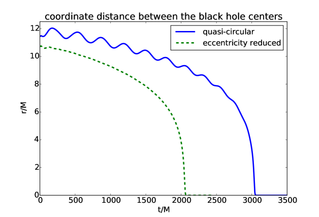
Figure 1: This plot shows the coordinate distance $r$ for two different binary black hole simulations versus time. In both cases the mass ratio is 3 and the spins are pointing along the orbital angular momentum with dimensionless spin magnitude of 0.4 for the smaller and 0.6 for the larger black hole. Both simulations are starting from puncture initial data, but with slightly different initial separations and black hole momenta. The solid line corresponds to the quasi-circular setup where we have only tangential momentum, chosen by the equality of Komar integral and ADM mass. The broken line is for data where we have added a small radial momentum and tuned the tangential momentum to obtain less eccentric orbits [80].

When we use Eq. (85) to choose the black hole momenta, we obtain quasi-circular initial data. These initial data can then be evolved to study the orbits of the black hole binaries. For both punctures and the superimposed Kerr-Schild initial data constructed within the CTS approach, we find that the orbits are reasonably circular inspiral orbits. The solid line in Fig. 1 shows the evolution of the coordinate distance between the two black holes when we start from puncture initial data and choose the initial momenta perpendicular to the line connecting the two black holes, and use the equality of Komar integral and ADM mass (discussed above) to determine the magnitude of the initial black hole momentum parameter. As we can see the distance between the two black holes is not monotonically decreasing during the inspiral due to some residual eccentricity. This can be explained by the fact that in this case the initial data are constructed in an approximation that assumes that the orbits are exactly circular, i.e. both black holes have only tangential momentum. Yet, in a real inspiral the black holes also have a small inward momentum component. This means the initial momenta are not the ones needed for a realistic inspiral situation. The situation can be improved if we also allow for a radial momentum component and adjust the tangential momentum magnitude. When this is done according to the prescription described in [80] we obtain an inspiral with much less eccentricity, as shown by the broken line in Fig. 1. By using such methods [81, 82, 83, 84, 85, 80] it is possible to achieve eccentricities on the order of $10^{-4}$ for puncture initial data.

As already mentioned, for initial data constructed within the CTS approach we also find eccentric orbits comparable to the solid line in Fig. 1, if we assume a helical Killing vector and construct orbits with only tangential velocity. The reason is again that a true inspiral does not have exactly a helical symmetry. However, as described in [51, 86] one can replace this helical symmetry by an inspiral symmetry, i.e. by assuming that the approximate Killing vector has the form

$$\xi_{insp}^{0} = 1,$$

$$\xi_{insp}^{i} = \Omega(-x^{2}+x_{CM}^{2},x^{1}-x_{CM}^{1},0)+\frac{v_{r}}{r_{12}}(x^{i}-x_{CM}^{i}),$$ (144)

where we have added a radial component to the helical vector and assume that orbital angular velocity is along the $x^{3}$-direction. Here $v_{r}$ is the radial velocity, $x_{CM}^{i}$ the center of mass position and $r_{12}$ the distance between the two black holes. We can now adjust $\Omega$ and $v_{r}$ to mimic true inspiral orbits. In comoving coordinates we still have

$$\xi^{\mu}=t^{\mu}=\alpha n^{\mu}+\beta^{\mu},$$ (145)

so that at spatial infinity the shift now must have the form

$$\lim_{r\to\infty}\beta^{i}=\xi_{insp}^{i}.$$ (146)

Within the CTS equations we can now use Eq. (146) as a boundary condition on the shift at $r\to\infty$. Using an iterative method [51, 86] it is possible to tune the values of $\Omega$ and $v_{r}$ to achieve very low eccentricities on the order of $5\times 10^{-5}$ [86] for conformally flat CTS initial data. Similar results can also obtained using superimposed Kerr-Schild CTS initial data [63]. In fact, this kind of eccentricity reduction works better for CTS based initial data than for CTT puncture initial data. The CTS decomposition gives us a direct handle on the shift (via Eq. (146)) and allows us to directly set certain time derivatives to zero. It produces a preferred lapse and shift that when used in the evolution, result in coordinates that are well adapted to quasi-equilibrium. For CTT based initial data one does not have such a preferred lapse and shift. Hence oscillations in the coordinate distance $r$ are not due to real eccentricity alone, but also due to the fact that the coordinates are still evolving as well. This problem is quite visible after eccentricity reduction in Fig. 1. The broken line shows a dip during the first $200M$ of the evolution. This non-monotonic behavior makes it harder to define or measure eccentricity, so that the reduction procedure works less well.

6 Toward more realistic binary black hole initial data

As discussed above, two orbiting black holes will emit gravitational radiation. From post-Newtonian calculations we expect to see a so called chirp signal during the inspiral phase, i.e. a gravitational wave with slowly increasing amplitude and frequency (see e.g. broken line in Fig. 2). The initial data should reflect this and contain such gravitational waves. However, when we construct conformally flat initial data using either the CTT or CTS approach, the resulting conformal factor will be monotonically decreasing as we move away from the black holes. Hence the 3-metric does not contain any wiggles. The same is true for the extrinsic curvature. This means that the initial slice of our spacetime contains no gravitational radiation at all, even though we have two orbiting black holes. This is clearly unrealistic, even though the data satisfy the constraints by construction. When such data are evolved in time the system starts to radiate and over time fills the spatial slice with gravitational waves.

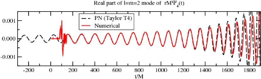
Figure 2: The solid line shows the gravitational waveform for a binary black hole simulation starting from puncture initial data with masses $m_{1}=0.25M$, $m_{2}=0.75M$ and spins of $S_{1}=0.4M^{2}$, $S_{2}=0.6M^{2}$ aligned with the orbital angular momentum. A post-Newtonian Taylor T4 waveform (broken line) has been matched to the numerical waveform by minimizing the difference in the time interval from $350M$ to $1100M$.

The results of a evolution starting from conformally flat puncture initial data is shown in Fig. 2. The solid line depicts the dominant mode of the Weyl scalar $\Psi_{4}$ which encodes the emitted gravitational waves. This mode has been extracted at a distance of about $90M$ from the center of mass. As we can see, there is no gravitational wave signal until disturbances from the black holes reach the extraction radius at a time of about $90M$. At this time we see a strong transient high frequency signal. This signal is usually referred to as junk radiation, since it is an artifact of the unrealistic initial data. The broken line shows the same mode computed from a corresponding post-Newtonian calculation, which contains no such junk radiation. Similar problems also occur for superimposed Kerr-Schild type data, because each individual black hole in the superposition is a stationary black hole solution of Einstein’s equations that does not contain any gravitational waves.

6.1 Post-Newtonian based initial data

We know that post-Newtonian calculations can be highly accurate during the inspiral phase before the black holes merge. This is also the regime in which we would like to construct initial data. It thus seems natural that we should try to incorporate post-Newtonian information into the initial data construction. Notice, however, that post-Newtonian theory is an approximation that assumes low velocities ($v/c\ll 1$) and weak gravity ($GM/r\ll 1$). While black holes may be moving slowly enough when they are still well separated, their gravitational fields are always strong near each black hole. For this reason post-Newtonian theory alone can give us reliable initial data only away from each black hole. In [87, 88] post-Newtonian initial data in ADMTT gauge [89] has been investigated. In this gauge one can directly obtain the 3-metric and the extrinsic curvature as post-Newtonian expansions. It is then possible to resum these expansion so that they take the form

$$\gamma^{PN}_{ij}=\psi_{PN}^{4}\delta_{ij}+h_{ij}^{TT}$$ (147)

and

$$K_{PN}^{ij}=\psi_{PN}^{-10}\left(\bar{A}_{BY}^{ij}+k^{ij}_{TT}\right)$$ (148)

with

$$\psi_{PN}=1+\sum_{A=1}^{2}\frac{E_{A}}{2r_{A}}.$$ (149)

Here $E_{A}$ are the energies of the point particles used in the post-Newtonian theory, $h_{ij}^{TT}$ and $k^{ij}_{TT}$ are higher order post-Newtonian terms that we do not write out here, and $\bar{A}_{BY}^{ij}$ is the Bowen-York extrinsic curvature given in Eq. (125) with $S_{A}^{i}=0$. As we can see the conformal factor is of Brill-Lindquist form as in Eq. (119). Thus these approximate initial data look very similar to puncture initial data. The main difference is the appearance of the extra terms $h_{ij}^{TT}$ and $k^{ij}_{TT}$, so that the 3-metric is no longer conformally flat. It is thus clear that these data do indeed contain black holes, even though the post-Newtonian expressions were derived using point particles. Following the approach in [87, 88] we can now construct constraint satisfying initial data by using the CTT decomposition with the free data

$$\bar{\gamma}_{ij} = \psi_{PN}^{-4}\gamma^{PN}_{ij}$$ (150)

$$\bar{M}^{ij} = \psi_{PN}^{10}\left(K_{PN}^{ij}-\frac{1}{3}\gamma_{PN}^{ij}K_{PN}\right)$$ (151)

$$K = 0$$ (152)

and using the puncture ansatz

$$\psi=\psi_{PN}+u$$ (153)

for the conformal factor. Inserting these expressions in Eqs. (42) and (44) we obtain elliptic equations for $u$ and $W^{i}$. These equations can be solved if we impose the boundary conditions

$$\lim_{r\to\infty}u=0$$ (154)

and Eq. (61). We then obtain initial data that satisfy Hamiltonian and momentum constraints. This was first done in [87] using a near zone approximation for the term $h_{ij}^{TT}$ in Eq. (147), but the full $h_{ij}^{TT}$ was later calculated in [88], and used to solve the constraints in [90]. As we can see from Eq. (153) the conformal factor gets modified when we solve for the constraint Eqs. (42) and (44). This leads in general to an increase in the ADM mass. Such changes are common when we use one of the conformal decompositions to find constraint satisfying data from approximate data. In [87] and [90] it was found that for the case of the post-Newtonian data in ADMTT gauge, this change in the mass can be prevented by also modifying the post-Newtonian conformal factor to

$$\psi_{PN}\to\psi_{PN}-q\frac{m_{1}m_{2}}{2r_{12}}\left(\frac{1}{2r_{1}}+\frac{1}{2r_{2}}\right).$$ (155)

This modification (parameterized by the number $q$) counters the effect of the term $u$ in Eq. (153) on the ADM mass. The parameter $q$ should be chosen such that the resulting initial data after solving the constraints in Eqs. (42) and (44) are as close as possible to the original post-Newtonian data. How exactly one best quantifies this closeness is still an open issue. A partial answer has been given e.g. in [87] where $q$ was chosen such that the binding energy after solving the constraints is as close as possible to the post-Newtonian binding energy.

In Fig. (3) we show the dominant $l=m=2$ mode of the gravitational waveform for different initial data.

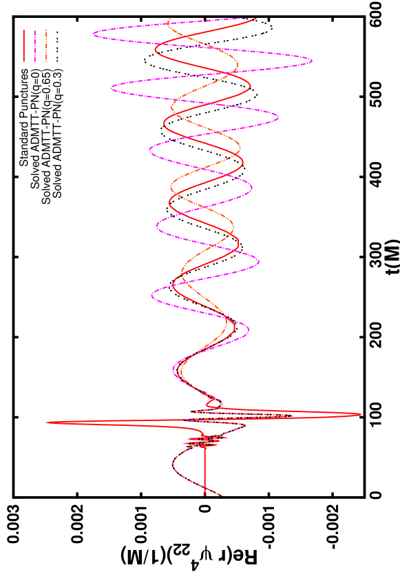
Figure 3: Results from the simulation of two non-spinning equal mass black holes starting from an initial coordinate separation of $10M$. The solid line shows the gravitational waveform for a binary black hole simulation starting from standard puncture initial data. Up to a time of about $t=90M$ we see no signal, because no waves are built into puncture data. After this time we see a strong junk signal. The other lines show the gravitational waveform when we start with post-Newtonian based initial data (with different values for the parameter $q$), where waves are built in from the start. These signals still contain junk radiation but with a reduced amplitude.

As we can see, the ADMTT based initial data leads to better waveforms with reduced junk radiation. Similar improvements in the waveform even exist if we do not solve the constraint equations and just directly use the approximate post-Newtonian data [91, 78].

6.2 Approximate initial data from matching

As we have seen, post-Newtonian theory can give very useful input when we want to construct initial data with gravitational waves already built into the initial slice. Yet, as discussed in the previous subsection, post-Newtonian theory is not valid near a black hole. In fact one had to judiciously resum the post-Newtonian expressions to even obtain black holes. These resummations were guided by the aim to make the post-Newtonian data similar to puncture initial data, because the latter contains well understood black holes. Of course this resummation is ad hoc, and it is not clear if we really obtain a good approximation near the black holes and whether the black holes are in equilibrium. In fact, since there is still some amount of junk radiation, we do know that they are not really equilibrium. For this reason an alternative method based on asymptotic matching has been proposed [92, 93, 94, 95]. In this method one matches a post-Newtonian 4-metric to two different perturbed black hole metrics (one for each black hole) to obtain an approximate solution everywhere. Then no ad hoc resummations are necessary, and we obtain an approximation that is valid everywhere. The most sophisticated data of this kind to date has been presented in [95], where a post-Newtonian 4-metric for circular orbits containing outgoing gravitational waves has been matched to two tidally perturbed Schwarzschild metrics. When we evolve initial data coming from this approximate 4-metric without solving the constraint equations, we find that the data have waves built in from the start and that there is less junk radiation than for puncture initial data [78]. However, somewhat surprisingly the junk radiation in the dominant $l=m=2$ mode has still about the same size as the one coming from the resummed ADMTT gauge post-Newtonian data discussed in the previous subsection, at least for a black hole separation of $10M$. However, further studies are necessary as it is likely that the situation will improve once we move the black holes further apart, since the then all the approximations used in the matching will improve.

In [96] the two tidally deformed black hole 4-metrics from [95] (but not the post-Newtonian 4-metric) have been used to construct a superposition as in Eqs. (136) and (137). This superposition thus contains black holes with the correct tidal deformations, but without any realistic gravitational waves, since the matched post-Newtonian 4-metric is not included. The constraint equations are then solved for this superposition following the methods described in Sec.5.4 within the CTS approach. The only difference is that as boundary condition at each black hole, [96] uses a Dirichlet condition for the shift, since tidally deformed black holes do not have a vanishing shear, so that Eq. (102) may not be appropriate. When these data are evolved, junk radiation is reduced when compared to conformally flat or superimposed Kerr-Schild data.

7 Matter equations for perfect fluids

So far we have been discussing how one can create initial data for vacuum solutions such as black holes. When we need initial data for situations where matter is involved, we have to consider additional equations that describe this matter. Here we will concentrate on matter that can be described as a perfect fluid. This is sufficient for e.g. neutron stars.

7.1 Perfect fluids

For a perfect fluid the stress-energy tensor is given by

$$T^{\mu\nu}=[\rho_{0}(1+\epsilon)+P]u^{\mu}u^{\nu}+Pg^{\mu\nu}.$$ (156)

Here $\rho_{0}$ is the mass density (which is proportional the number density of baryons), $P$ is the pressure, $\epsilon$ is the internal energy density divided by $\rho_{0}$ and $u^{\mu}$ is the 4-velocity of the fluid. The matter variables in Eq.(2.4) are then

$$\rho = \alpha^{2}[\rho_{0}(1+\epsilon)+P]u^{0}u^{0}-P$$

$$j^{i} = \alpha[\rho_{0}(1+\epsilon)+P]u^{0}u^{0}(u^{i}/u^{0}+\beta^{i})$$

$$S^{ij} = [\rho_{0}(1+\epsilon)+P]u^{0}u^{0}(u^{i}/u^{0}+\beta^{i})(u^{j}/u^{0}+\beta^{j})+P\gamma^{ij},$$ (157)

where $u^{0}=-n_{\mu}u^{\mu}/\alpha$.

From $\nabla_{\nu}T^{\mu\nu}=0$ we obtain the relativistic Euler equation

$$[\rho_{0}(1+\epsilon)+P]u^{\nu}\nabla_{\nu}u^{\mu}=-(g^{\mu\nu}+u^{\mu}u^{\nu})\nabla_{\nu}P,$$ (158)

which together with the continuity equation

$$\nabla_{\nu}(\rho_{0}u^{\nu})=0$$ (159)

governs the fluid. The five fluid Eqs. (158) and (159) are not enough to determine the the six quantities $\rho_{0}$, $\epsilon$, $P$ and $u^{i}$. We thus also need an equation of state of the form

$$P=P(\rho_{0},\epsilon)$$ (160)

to close the system of fluid equations. In many cases it is also useful to introduce the specific enthalpy

$$h=1+\epsilon+P/\rho_{0},$$ (161)

because then the Euler equation can be simplified to

$$u^{\nu}\nabla_{\nu}(hu_{\mu})+\nabla_{\mu}h=0.$$ (162)

Using $u^{\mu}u_{\mu}=-1$, the latter can also be written as

$$\vec{u}\cdot d\undertilde{p}=0.$$ (163)

Here $\vec{u}$ is the fluid velocity 4-vector and the one-form $\undertilde{p}$ has the components

$$p_{\mu}=hu_{\mu}.$$ (164)

The dot in Eq. (163) indicates contraction of the vector $\vec{u}$ with the first index of the two-form $d\undertilde{p}$.

7.2 Expansion, shear and rotation of a fluid

Using the projector

$$P_{\mu\nu}=g_{\mu\nu}+u_{\mu}u_{\nu},$$ (165)

covariant derivatives of the fluid 4-velocity we can be split into

$$\nabla_{\nu}u_{\mu}=\frac{1}{3}\theta P_{\mu\nu}+\varsigma_{\mu\nu}+\omega_{\mu\nu}-a_{\mu}u_{\nu},$$ (166)

where the expansion, shear, rotation and acceleration of the fluid are defined as

$$\theta=P^{\mu\nu}\nabla_{\mu}u_{\nu},$$ (167)

$$\varsigma_{\mu\nu}=P_{\mu}^{\mu^{\prime}}P_{\nu}^{\nu^{\prime}}\nabla_{(\mu^{\prime}}u_{\nu^{\prime})}-\frac{1}{3}\theta P_{\mu\nu},$$ (168)

$$\omega_{\mu\nu}=P_{\mu}^{\mu^{\prime}}P_{\nu}^{\nu^{\prime}}\nabla_{[\nu^{\prime}}u_{\mu^{\prime}]}$$ (169)

and

$$a_{\mu}=u^{\nu}\nabla_{\nu}u_{\mu}.$$ (170)

If the 4-velocity is of the form

$$u^{\mu}=f\tilde{u}^{\mu},$$ (171)

where $f$ is any scalar function, it immediately follows from $P_{\mu\nu}u^{\nu}=0$ that

$$\theta=fP^{\mu\nu}\nabla_{\mu}\tilde{u}_{\nu},$$ (172)

$$\varsigma_{\mu\nu}=fP_{\mu}^{\mu^{\prime}}P_{\nu}^{\nu^{\prime}}\nabla_{(\mu^{\prime}}\tilde{u}_{\nu^{\prime})}-\frac{1}{3}\theta P_{\mu\nu},$$ (173)

$$\omega_{\mu\nu}=fP_{\mu}^{\mu^{\prime}}P_{\nu}^{\nu^{\prime}}\nabla_{[\nu^{\prime}}\tilde{u}_{\mu^{\prime}]}.$$ (174)

From the latter is is clear that if the velocity is derived from a potential $\phi$, i.e. if $h\undertilde{u}=\undertilde{p}=d\phi$, we immediately obtain $\omega_{\mu\nu}=0$, which characterizes an irrotational fluid.

8 Single neutron stars

8.1 Non-spinning neutron stars

Let us consider a static spherically symmetric star. In this case the Einstein equations can be solved exactly. The metric outside the star is given by the Schwarzschild metric of Eq. (103), but with $m$ replaced by $m(r_{s*})$, where $r_{s*}$ is the star radius (in standard Schwarzschild coordinates) and

$$m(r_{s})=\int_{0}^{r_{s}}dr^{\prime}4\pi r^{\prime 2}\rho_{E}$$ (175)

is the gravitational mass inside radius $r_{s}$ and

$$\rho_{E}=\rho_{0}(1+\epsilon).$$ (176)

Inside the star the metric is given by

$$ds^{2}=-e^{2\phi}dt^{2}+(1-2m(r_{s})/r_{s})^{-1}dr_{s}^{2}+r_{s}^{2}(d\theta^{2}+\sin^{2}\theta d\phi^{2}),$$ (177)

where $m(r_{s})$, $\Phi(r_{s})$ and also $P(r_{s})$ are found by integrating the Tolman-Oppenheimer-Volkoff (TOV) equations [97, 98]

$$\frac{dm}{dr_{s}} = 4\pi r_{s}^{2}\rho_{E}$$ (178)

$$\frac{dP}{dr_{s}} = -\frac{(\rho_{E}+P)(m+4\pi r_{s}^{3}P)}{r_{s}(r_{s}-2m)}$$ (179)

$$\frac{d\Phi}{dr_{s}} = \frac{m+4\pi r_{s}^{3}P}{r_{s}(r_{s}-2m)}$$ (180)

together with some equation of state that allows us to obtain $\rho_{E}$ from $P$. The TOV equations are ordinary differential equations that have to be integrated out from $r_{s}=0$ to the radius where $P=0$, which is the location of the star surface ($r_{s}=r_{s*}$). At $r_{s}=0$ we start with $m=0$ and some value of $P=P_{c}$ which determines the core pressure and thus the total mass of the star. We also have to start with some particular $\Phi$ at $r_{S}=0$. We can set this value to 1 at first. The final $\Phi(r)$ can be obtained by adding a constant to it such that $2\Phi(r_{s*})=\ln(1-2m(r_{s*})/r_{s*})$. This shift in $\Phi$ ensures that the metric is continuous at the star surface. It is possible, and often convenient, to transform the TOV metric to isotropic coordinates by using the transformation given in Eqs. (104) and (105). From the TOV metric it is then easy to obtain the 3-metric and extrinsic curvature.

8.2 Spinning neutron stars

The metric for a spinning neutron star is no longer spherically symmetric. Instead one assumes a stationary and axisymmetric metric of the form

$$ds^{2}=-e^{A+B}dt^{2}+e^{2C}(dr^{2}+r^{2}d\theta^{2})+e^{A-B}r^{2}\sin^{2}\theta(d\phi-\omega dt)^{2},$$ (181)

where $A$, $B$, $C$ and $\omega$ are functions of $r$ and $\theta$ only. If matter is again treated as a perfect fluid and an equation of state is provided, one obtains a system of three field equations and one equation expressible as a line integral [99], both inside the star and in the vacuum region on the outside. This system of equations is rather complicated and we will not go through its derivation here. It can only be solved numerically. Several groups have worked on this problem in the past. A freely available public code (called RNS) that can solve the system of equations has been developed by Stergioulas and Friedman [100]. However, the most accurate results by far have been achieved by Ansorg et al. [99, 101]. It is also worth mentioning that the metric outside a spinning star is not given by the Kerr metric that is valid for a rotating black hole. A review about a single spinning neutron stars can be found in [102].

9 Binary neutron star initial data

Binary neutron stars, like binary black holes, will be on approximately circular orbits if they have been inspiraling already for a long time. We can thus use many of the same methods as for black holes when we construct binary neutron star initial data. Thus again we can assume that an approximate helical or inspiral Killing vector $\xi^{\mu}$ as in Eq. (5.7) should exist. So again we can choose coordinates where Eq. (80) holds, and in which time derivatives of metric variables can be approximated by zero. As mentioned previously, such a situation can be captured best by using the CTS decomposition, which we will use almost exclusively for the binary neutron star initial data described below. We will also restrict ourselves to the case of a conformally flat metric as in Eq. (117). Since gravity in neutron stars is weaker and rotational velocities are lower than in black holes, conformal flatness is generally a good approximation for neutron stars. Notice however, that a very interesting non-conformally flat method, named the waveless formulation, has been developed [103, 104, 105, 106]. In this formulation one obtains the same fluid equations as described below. The equations for the metric variables are essentially the CTS equations, plus one additional elliptic equation for the conformal metric. This extra equation is derived from the evolution equation for the extrinsic curvature by using a particular gauge to rewrite $R_{ij}$ in Eq. (29) as an elliptic operator acting on the conformal metric. Thus the conformal metric does not need to be assumed to be of a particular form, rather it is computed from the additional elliptic equation. Instead one needs to specify as free data the time derivative of a conformally rescaled tracefree extrinsic curvature, in addition to the time derivative of the conformal metric.

The main difference between binary neutron star initial data and binary black hole initial data is that we now also have to find quasi-equilibrium configurations for the matter, when we solve the Euler and continuity equations in Eqs. (158) and (159). Notice, however, that the stars have only a finite extent so that we will use the same boundary conditions for the metric variables as in Sec. 3.3 at infinity.

As in the black hole case, we will not discuss every possible method to construct binary neutron star initial data here. Rather we will concentrate on conceptual issues, as well as on describing the most widely used methods.

9.1 Corotating binary neutron stars

In order to construct initial data for two neutron stars in a corotating configuration, we assume again a helical Killing vector $\xi^{\mu}$. The fact that the two stars are corotating means that the orbital period and both star spin periods all have the same value. Thus each fluid element is at rest in corotating coordinates. This idea is captured by assuming that the fluid in each star flows along the Killing vector $\xi^{\mu}$, i.e. that the fluid 4-velocity is

$$u^{\mu}=u^{0}\xi^{\mu}.$$ (182)

In this case it is easy to show that the continuity equation (159) is identically satisfied. Furthermore one can show that the Euler equation leads to (see e.g. problem 16.17 in [107])

$$[\rho_{0}(1+\epsilon)+P]d\ln(u_{\mu}\xi^{\mu})=-dP,$$ (183)

where $\xi^{\mu}$ is the assumed helical Killing vector. With the help of the first law of thermodynamics ($d[\rho_{0}(1+\epsilon)]=[\rho_{0}(1+\epsilon)+P]d\rho_{0}/\rho_{0}$) this equation can be integrated to yield

$$u_{\mu}\xi^{\mu}=\frac{C\rho_{0}}{\rho_{0}(1+\epsilon)+P},$$ (184)

where $C$ is a constant of integration that is different for each star. Using Eqs. (182) and (161) we arrive at

$$h=-Cu^{0},$$ (185)

which tells us the value of the specific enthalpy for each point inside the star.

If we assume a polytropic equation of state

$$P=\kappa\rho_{0}^{1+1/n},$$ (186)

we can express the mass density, the pressure and the internal energy in terms of $h$. We obtain

$$\rho_{0} = \kappa^{-n}\left(\frac{h-1}{n+1}\right)^{n}$$

$$P = \kappa^{-n}\left(\frac{h-1}{n+1}\right)^{n+1}$$

$$\epsilon = n\left(\frac{h-1}{n+1}\right).$$ (187)

The constant $n$ here is known as the polytropic index, and $\kappa$ is a constant.

In order to construct binary neutron star initial data we have to solve the five elliptic equations in Eqs. (42), (52) and (56) with the matter terms given by Eqs. (7.1), (185) and (9.1). This is done through an iterative procedure [108] as described in subsection 9.4.

Examples of such corotating initial data can be found in [109, 110, 111, 112, 108]. The problem with such data is that it is very unlikely for two neutron stars to have spin periods that are both synchronized with the orbital period. As pointed out by Bildsten and Cutler [113], the two neutron stars cannot be tidally locked, because the viscosity of neutron star matter is too low. Hence barring other effects, like magnetic dipole radiation, the spin of each star remains approximately constant. This means that initial data sequences of corotating configurations for different separations cannot be used to approximate the inspiral of two neutron stars.

9.2 Irrotational binary neutron stars

Since corotating configurations are unrealistic, many groups use initial data for irrotational stars. The advantage is that, sequences of irrotational configurations can be used to approximate the inspiral of two neutron stars without spin. Of course, for such configurations the fluid velocity will not be along the helical Killing vector, which we will still assume to exist approximately. Thus the fluid velocity is now written as

$$u^{\mu}=u^{0}\left(\xi^{\mu}+V^{\mu}\right),$$ (188)

where $u^{0}=-u^{\mu}n_{\mu}/\alpha$, and $V^{\mu}$ is a purely spatial vector with $V^{\mu}n_{\mu}=0$ that describes the fluid velocity relative to the Killing vector $\xi^{\mu}$.

In order to find the enthalpy for a quasi-equilibrium situation we insert Eq. (188) into Euler Eq. (163) to obtain

$$\vec{\xi}\cdot d\undertilde{p}+\vec{V}\cdot d\undertilde{p}=0.$$ (189)

Note that for any vector $\vec{v}$ and form $\undertilde{\omega}$ the Cartan identity

$$\pounds_{v}\undertilde{\omega}=\vec{v}\cdot d\undertilde{\omega}+d(\vec{v}\cdot\undertilde{\omega})$$ (190)

holds, where $\pounds_{v}\undertilde{\omega}$ is the Lie derivative of $\undertilde{\omega}$ along $\vec{v}$. The dot in Eq. (190) indicates contraction of a vector with the first index of a form. Using the Cartan identity to replace $\vec{\xi}\cdot d\undertilde{p}$, Eq. (189) simplifies to

$$\pounds_{\xi}\undertilde{p}-d(\vec{\xi}\cdot\undertilde{p})+\vec{V}\cdot d\undertilde{p}=0.$$ (191)

The first term in this equation term will be dropped since $\vec{\xi}$ is an approximate Killing vector, i.e.

$$\pounds_{\xi}\undertilde{p}=\pounds_{t}\undertilde{p}\approx 0,$$ (192)

where we again have used corotating coordinates as in Eq. (80).

From Eq. (163) we can see that setting

$$\undertilde{p}=d\phi$$ (193)

will automatically solve the Euler equation. The function $\phi$ is a velocity potential from which we can then derive $p_{\mu}=hu_{\mu}$. Notice that a fluid with a velocity coming from a potential, according to $hu_{\mu}=\nabla_{\mu}\phi$, has zero rotation (see Eqs. (171) and (174)), hence the name irrotational configuration for the initial data constructed in this section.

If we insert Eq. (193) together with assumption (192) into Eq. (191) we finally obtain

$$d(\vec{\xi}\cdot\undertilde{p})=0,$$ (194)

which implies that

$$hu_{\mu}\xi^{\mu}=C,$$ (195)

where $C$ is a constant that may be different in each star. Inserting $\xi^{\mu}=u^{\mu}/u^{0}-V^{\mu}$ from Eq. (188) and using $u_{\mu}u^{\mu}=-1$ we arrive at

$$\frac{h}{u^{0}}+V^{k}D_{k}\phi=-C$$ (196)

As in the case of corotating configurations this last equation can be used to find the specific enthalpy. Note that $u^{0}$ can be obtained from $u_{\mu}u^{\mu}=-1$.

Using Eqs. (188) and (193) one can show that the continuity equation (159) becomes [114, 115, 116]

$$D_{i}\left[\frac{\rho_{0}\alpha}{h}D^{i}\phi-\rho_{0}\alpha u^{0}(\beta^{i}+\xi^{i})\right]=0,$$ (197)

where we have again dropped some Lie derivatives with respect to the Killing vector $\vec{\xi}$. More details about this derivation will be provided in the next section, where we consider the more general case of spinning stars. Compared to the corotating configuration, the irrotational case yields the additional elliptic Eq. (197), that we need to solve for the velocity potential $\phi$ together we the other elliptic equations for the metric variables in Eqs. (42), (52), (56). Such irrotational binary neutron stars have been produced by many groups [117, 118, 119, 120, 121, 122, 123, 124, 125, 126].

9.3 Binary neutron stars with arbitrary spins

We will now consider the general case of neutron stars with spin. First we assume that the binary is in an approximately circular orbit and that the spin of each star remains approximately constant. As in the case of binary black holes (see e.g. [31, 37]) this implies the existence of an approximate helical Killing vector $\xi^{\mu}$ with $\pounds_{\xi}g_{\mu\nu}\approx 0$. In order to clarify the meaning of the approximate sign we now briefly discuss two cases.

If both star spins are parallel to the orbital angular momentum we have $\pounds_{\xi}g_{\mu\nu}=O(P_{o}/T_{ins})$, where the inspiral timescale $T_{ins}$ is much longer than the orbital timescale $P_{o}$. I.e. in a corotating coordinate system all metric time derivatives are of order $O(P_{o}/T_{ins})$ and thus small. For arbitrary spins the situation becomes more complicated. We can again use corotating coordinates, but in this coordinate system the spin vectors will be precessing on an orbital timescale $P_{o}$. This means there are matter currents that change on a timescale $P_{o}$, and thus $\pounds_{\xi}u_{\mu}$ cannot be zero [116] even approximately! On the other hand, the matter distribution itself only changes on the much longer inspiral timescale $T_{ins}$. In this case it is useful to consider gravity to be made up of gravitoelectric and gravitomagnetic fields [127, 15]. The gravitoelectric parts of the metric are sourced by the matter distribution and thus change only on the timescale $T_{ins}$, while the gravitomagnetic parts of the metric are sourced by matter currents and thus change on the shorter timescale $P_{o}$. However, the gravitomagnetic parts are smaller than the gravitoelectric parts by $O(v/c)$ [127, 15]. Thus we now have $\pounds_{\xi}g_{\mu\nu}=O(v/c)\approx 0$, where we assume that the orbital velocity $v$ is smaller than the speed of light.

We start again by writing the fluid velocity as in Eq. (188) and use again the Cartan identity to bring the Euler equation into the form in Eq. (191). However, this time we cannot assume that $\pounds_{\xi}\undertilde{p}$ is zero. Also, since both stars are spinning, the fluid flow is no longer purely irrotational, so that now we write

$$h\undertilde{u}=\undertilde{p}=d\phi+\undertilde{w},$$ (198)

where $d\phi$ and $\undertilde{w}$ denote the irrotational and rotational pieces of the velocity. Here $\undertilde{w}$ is chosen to be purely spatial, i.e. such that $\vec{n}\cdot\undertilde{w}=0$. It is clear that $d\phi$ describes the orbital or center of mass motion of the star, while $\undertilde{w}$ is due to the star spin.

Using Eq. (198) together with the Cartan identity (190), the last term in Eq. (191) becomes

$$\vec{V}\cdot d\undertilde{p}=\vec{V}\cdot d\undertilde{w}=\pounds_{V}\undertilde{w}-d(\vec{V}\cdot\undertilde{w})$$ (199)

so that Eq. (191) is equivalent to

$$d(\vec{\xi}\cdot\undertilde{p}+\vec{V}\cdot\undertilde{w})=\pounds_{\xi}(d\phi+\undertilde{w})+\pounds_{V}\undertilde{w}=\pounds_{\xi}d\phi+\pounds_{\xi+V}\undertilde{w}.$$ (200)

Notice that according to Eqs. (188) and (198)

$$\vec{\xi}+\vec{V}=\frac{1}{hu^{0}}(\vec{\nabla}\phi+\vec{w})$$ (201)

so that Eq. (200) finally becomes

$$d(\vec{\xi}\cdot\undertilde{p}+\vec{V}\cdot\undertilde{w})=\pounds_{\xi}d\phi+\pounds_{\frac{\nabla\phi}{hu^{0}}}\undertilde{w}+\pounds_{\frac{w}{hu^{0}}}\undertilde{w}.$$ (202)

Following [116], we will now argue that all three terms on the right hand side of Eq. (202) are small. Since the center of mass motion described by $d\phi$ should be unchanged along the approximate symmetry vector $\vec{\xi}$, we will assume that

$$\pounds_{\xi}d\phi\approx 0.$$ (203)

As we have explained, the spin and thus $\undertilde{w}$ changes along $\vec{\xi}$. However, if we go along the center of mass direction given by $\vec{\nabla}\phi$, we expect the spin to be unchanged. Thus we assume

$$\pounds_{\frac{\nabla\phi}{hu^{0}}}\undertilde{w}\approx 0.$$ (204)

Furthermore we assume that

$$\pounds_{\frac{w}{hu^{0}}}\undertilde{w}\approx 0,$$ (205)

which tells us that the spinning motion of the star does not change if we go along the direction of this spinning motion.

Figure 4: Schematic picture of a star and its spin $S$: The star starts on the bottom and then moves along a circular arc. Its center follows the Killing vector $\vec{\xi}$. The star spin $S$ is approximately unchanged over an orbital timescale. The point $P$ becomes point $P^{\prime}$ if we follow the orbit of the Killing vector, while it becomes point $Q$ if we follow the center of mass motion parallel to $\vec{\nabla}\phi$. The orbital fluid speed (excluding the spin) at $P$ and $P^{\prime}$ are the same. Yet, the fluid motion due to the spin at $P^{\prime}$ is not the same as at $P$. Rather it should be approximately the same as at $P$ and $Q$.

The foregoing argument is also illustrated in Fig. 4, which schematically depicts the star over a quarter orbit. As the star moves, its spin stays approximately constant and its center moves along the Killing vector $\vec{\xi}$. If we start at point $P$ and follow $\vec{\xi}$ we end up at point $P^{\prime}$. If instead we follow the center of mass motion parallel to $\vec{\nabla}\phi$ we arrive at $Q$. As we can see the orbital fluid speed (excluding the spin) at $P$ and $P^{\prime}$ are the same, which is the origin of assumption 203. However, the fluid motion due to the spin at $P$ and $P^{\prime}$ are not the same. Rather we expect the spin motion to be approximately the same at point $P$ and $Q$, which supports assumption 204.

Using the three assumptions in Eqs. (203), (204) and (205), we can integrate Eq. (202) and obtain

$$C=\vec{\xi}\cdot\undertilde{p}+\vec{V}\cdot\undertilde{w}=\left(\frac{\vec{u}}{u^{0}}-\vec{V}\right)\cdot h\undertilde{u}+\vec{V}\cdot\undertilde{w}=-\frac{h}{u^{0}}-V^{i}D_{i}\phi,$$ (206)

where $C$ is the constant of integration. This last equation is again used to find $h$. It reduces to Eq. (185) in the corotating case where $\vec{V}=0$, and has exactly the same form as Eq. (196) for the irrotational case. In order to to find $u^{0}$ we use

$$-1=\vec{u}\cdot\undertilde{u}=(\gamma^{\mu\nu}-n^{\mu}n^{\nu})u_{\mu}u_{\nu}=\gamma^{\mu\nu}u_{\mu}u_{\nu}-(n_{0}u^{0})^{2}.$$ (207)

We now multiply by $h^{2}$, use Eq. (198) and solve for $u^{0}$. We find

$$u^{0}=\sqrt{h^{2}-(D_{i}\phi+w_{i})(D^{i}\phi+w^{i})}/(h\alpha).$$ (208)

If we insert Eq. (208) into the integrated Euler equation (206) we can solve for $h$. This yields

$$h=\sqrt{L^{2}-(D_{i}\phi+w_{i})(D^{i}\phi+w^{i})},$$ (209)

where we use the abbreviations

$$L^{2}=\frac{b+\sqrt{b^{2}-4\alpha^{4}[(D_{i}\phi+w_{i})w^{i}]^{2}}}{2\alpha^{2}}$$ (210)

and

$$b=[(\xi^{i}+\beta^{i})D_{i}\phi-C]^{2}+2\alpha^{2}(D_{i}\phi+w_{i})w^{i}.$$ (211)

We now rewrite the continuity Eq. (159) as

$$0 = g^{\mu\nu}\nabla_{\mu}[\rho_{0}u^{0}(\xi_{\nu}+V_{\nu})]=(\xi^{\mu}+V^{\mu})\nabla_{\mu}(\rho_{0}u^{0})+\rho_{0}u^{0}[g^{\mu\nu}(\nabla_{\mu}\xi_{\nu}+\nabla_{\mu}V_{\nu})]$$ (212)

$$= \pounds_{\xi}(\rho_{0}u^{0})+V^{i}D_{i}(\rho_{0}u^{0})+\rho_{0}u^{0}[g^{\mu\nu}\pounds_{\xi}g_{\mu\nu}+(\gamma^{\mu\nu}-n^{\mu}n^{\nu})\nabla_{\mu}V_{\nu}]$$

$$= \pounds_{\xi}(\rho_{0}u^{0})+V^{i}D_{i}(\rho_{0}u^{0})+\rho_{0}u^{0}[g^{\mu\nu}\pounds_{\xi}g_{\mu\nu}+D_{i}V^{i}+V^{\nu}n^{\mu}\nabla_{\mu}n_{\nu}.$$

Using Eq. (27) and collecting terms we obtain

$$D_{i}(\alpha\rho_{0}u^{0}V^{i})+\alpha\pounds_{\xi}(\rho_{0}u^{0})+\alpha\rho_{0}u^{0}g^{\mu\nu}\pounds_{\xi}g_{\mu\nu}=0.$$ (213)

Since $\vec{\xi}$ is an approximate Killing vector we can drop the last term. We also assume that

$$\pounds_{\xi}(\rho_{0}u^{0})\approx 0$$ (214)

since the matter density should be constant along the symmetry vector $\vec{\xi}$. As we can see Eq. (213) is identically satisfied in the corotating case where $V^{i}=0$. For all other cases Eq. (213) can be turned into an elliptic equation for $\phi$. To do this, first notice that combining Eqs. (188) and (198) yields

$$\vec{V}=\frac{\vec{\nabla}\phi+\vec{w}}{hu^{0}}-\vec{\xi}.$$ (215)

If we project this equation onto the spatial slice using $\gamma^{\mu}_{\nu}$ we find

$$V^{i}=\frac{D^{i}\phi+w^{i}}{hu^{0}}-(\xi^{i}+\beta^{i}).$$ (216)

When the latter is inserted into Eq. (213) we obtain

$$D_{i}\left[\frac{\rho_{0}\alpha}{h}(D^{i}\phi+w^{i})-\rho_{0}\alpha u^{0}(\beta^{i}+\xi^{i})\right]=0.$$ (217)

Notice that this expression reduces to Eq. (197) in the irrotational case where $w^{i}=0$.

Equation (217) is only valid inside the star and we have to provide a boundary condition at the star surface where $\rho_{0}=0$. This condition can be obtained directly from Eq. (217) in the limit of $\rho_{0}\to 0$ but $D_{i}\rho_{0}\neq 0$. We find [116]

$$(D^{i}\phi)D_{i}\rho_{0}+w^{i}D_{i}\rho_{0}=hu^{0}(\beta^{i}+\xi^{i})D_{i}\rho_{0}.$$ (218)

Notice that the rotational velocity piece $w^{i}$ can be freely chosen. In [128] it is demonstrated that

$$w^{i}=\epsilon^{ijk}\omega^{j}(x^{k}-x^{k}_{C*})$$ (219)

is a good choice, that results in almost rigidly rotating fluid configurations with low expansion and shear. Here $x^{k}_{C*}$ denotes the location of the star center and $\omega^{j}$ is an arbitrarily chosen vector that determines the star spin. Summation over the repeated indices $j$ and $k$ is implied

To close the system of equations we need again an equation of state. The simplest choice is the polytrope given in Eq. (186), which again results in Eqs. (9.1). However, other choices are possible. For example, [129] uses piecewise polytropic equations of state to approximate several realistic equations of state at zero temperature.

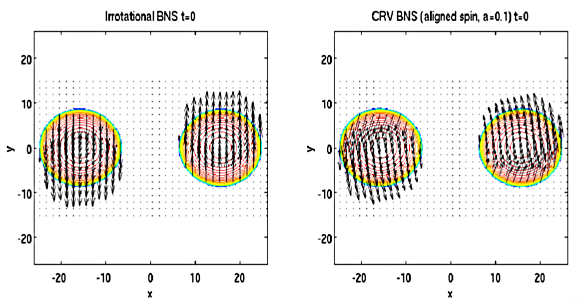
Figure 5: Two examples of binary neutron star initial data. Shown are contour lines of the density and the velocity vectors of fluid elements in the orbital plane. For an irrotational binary (left plot) the fluid velocity is perpendicular to the line connecting the star centers. For counterclockwise spinning stars (right plot) the fluid velocity is modified due to the additional rotational piece $w^{i}$ in Eq. (198).

Figure 5 shows velocity vectors of fluid elements in the orbital plane for two binaries. In the irrotational case (on the left) the fluid velocity is in the orbital direction. For the case where both stars are spinning (right plot) the fluid velocity has an additional rotational contribution due to $w^{i}$ in Eq. (198).

The same set of equations discussed above has also been used in [130, 131]. Notice, however, that [130] erroneously assumes $\pounds_{\xi}\undertilde{p}=0=\pounds_{V}\undertilde{w}$. But as shown in the appendix of [116], $\pounds_{\xi}\undertilde{p}$ cannot be approximately zero for generic spins. Fortunately the two errors incurred by the latter two assumptions cancel, so that the right hand side of Eq. (200) is again zero, and all other equations follow as shown above.

Spinning binary neutron initial data constructed with the method described above are evolved in [131], and the star spins are monitored using a newly defined quasi-local neutron star spin. It is found that the star spins follow post-Newtonian predictions during the inspiral of the two stars. This indicates that the above formalism together with the choice for $w^{i}$ in Eq. (219) works and results in realistic star spins.

9.4 Iteration procedures required to construct binary neutron star initial data

As we have discussed above, the construction of binary neutron star initial data requires us to solve the elliptic equations of the CTS approach in Eqs. (42), (52) and (56) coupled to the matter equations which are given by Eqs. (217) and (209) for stars in general rotation states or only Eq. (185) for corotating configurations. Both Eq. (209) and Eq. (185) are algebraic equations that specify the specific enthalpy $h$ given the other fields that obey elliptic equations. The situation is complicated by the fact that the star surfaces are at the location where $h=1$, so that one cannot know where the star surfaces will be before solving all coupled equations. Thus we do not know in which regions we indeed have to include matter terms in Eqs. (42), (52) and (56). Notice also that the values of the matter terms are undefined if we blindly use the equation of state in regions where $h<1$ (see e.g. Eqs. (9.1)).

For these reasons the Eqs. (42), (52), (56), (217) and (209) are solved using an iterative procedure [128], that can be outlined as follows: (i) We first come up with an initial guess for $h$ in each star (in practice we often choose Tolman-Oppenheimer-Volkoff solutions). (ii) Next, we solve the 6 coupled elliptic equations in Eqs. (42), (52), (56) and (217) for this given $h$. (iii) Then we use Eq. (209) to update $h$ in each star. After updating $h$ we go back to step (ii) and iterate until all equations are satisfied up to a given tolerance.

There is however one major ingredient missing in the above outline. Our entire method assumes a symmetry vector $\vec{\xi}$ of the form (5.7). Thus we need particular values for $\Omega$ and $x_{CM}^{1}$. Now, the star surfaces move between iteration steps. If we simply specify constant values for $\Omega$ and $x_{CM}^{1}$, it turns out that the stars drift away and that the iteration becomes unstable. We thus have to find a way to keep the stars from drifting. This is usually done by adjusting $\Omega$ and $x_{CM}^{1}$ such that the star center does not move when we update $h$ using Eq. (209). Notice that Eq. (209) depends on $\Omega$ and $x_{CM}^{1}$ through $\xi^{i}$ which is contained in $b$ from Eq. (211). The star centers $x_{C*1/2}^{1}$ are defined by the maxima of $h$ along the $x^{1}$-axis, given by $\partial_{1}h|_{x_{C*1/2}^{1}}=0$. In [128, 129] it is shown that the latter can be expressed as

$$\partial_{1}\ln\left[\alpha^{2}-\left(\beta^{i}+\xi^{i}+\frac{w^{i}}{hu^{0}}\right)\left(\beta_{i}+\xi_{i}+\frac{w_{i}}{hu^{0}}\right)\right]\Bigg{|}_{x_{C*1/2}^{1}}=-2\partial_{1}\ln\Gamma\big{|}_{x_{C*1/2}^{1}}$$ (220)

where

$$\Gamma=\frac{\alpha u^{0}\left[1-\left(\beta^{i}+\xi^{i}+\frac{w^{i}}{hu^{0}}\right)\frac{D_{i}\phi}{\alpha^{2}hu^{0}}-\frac{w_{i}w^{i}}{(\alpha hu^{0})^{2}}\right]}{\sqrt{1-\left(\beta^{i}+\xi^{i}+\frac{w^{i}}{hu^{0}}\right)\left(\beta_{i}+\xi_{i}+\frac{w_{i}}{hu^{0}}\right)\frac{1}{\alpha^{2}}}}.$$ (221)

We then update $\Omega$ and $x_{CM}^{1}$ by solving Eq. (220) for $\Omega$ and $x_{CM}^{1}$ so that the star centers $x_{C*1/2}^{1}$ remain in the same location, when we update $h$ according to Eq. (209). Equation (220) is often called the force balance equation [118]. One noteworthy caveat is that we evaluate the derivative of $\ln\Gamma$ in Eq. (220) for the $\Omega$ and $x_{CM}^{1}$ before the update.

Finally, the complete iteration procedure involves the following main steps [128]: (1) We first come up with an initial guess for $h$ in each star, in practice we often choose Tolman-Oppenheimer-Volkoff solutions for each. (2) Next, we solve the 6 coupled elliptic equations in Eqs. (42), (52), (56) and (217) for this given $h$. (3) We adjust $\Omega$ and $x_{CM}^{1}$ using the force balance Eq. (220). (4) Then we use Eq. (209) to update $h$ in each star. The constant $C$ has a different value for each star. We adjust the value for each star such that it keeps a prescribed rest mass. After updating $h$ we go back to step (2) and iterate until all equations are satisfied up to a given tolerance.

Notice however, that sometimes other conditions are used instead of the force balance Eq. (220). As first found in [125], for massive stars in can be helpful to determine $x_{CM}^{1}$ by demanding that the ADM linear momentum be zero [132, 133, 129, 126].

9.5 General orbits and low eccentricity orbits

If we evolve the quasi-circular (i.e. with $v_{r}=0$ in Eq. (5.7)) binary neutron star initial data described in the previous sections, we find that the orbits are roughly circular inspiral orbits. However, as in the case of black holes (see e.g. Fig. 1), the distance between the stars exhibits small oscillations, which are a sign of residual eccentricity caused by our assumption of exactly circular orbits. As for black holes, we would like to adjust $\Omega$ and $v_{r}$ in Eq. (5.7), to obtain less eccentric orbits when we evolve such initial data. There is, however, one immediate problem. The value of $\Omega$ is determined by the force balance Eq. (220), and thus cannot be readily changed.

In [134] a method has been developed that lets us construct orbits with arbitrary eccentricity. The extra parameter $e$ describing this eccentricity can then be adjusted along with $v_{r}$ to find low eccentricity orbits when the data are evolved. We now describe how the symmetry vector $\xi^{\mu}$ can be modified to account for non-circular orbits. We make the following two assumptions: (i) $\xi^{\mu}$ is along the motion of the star center. (ii) Without inspiral, each star center moves along a segment of an elliptic orbit at apoapsis. Since we only need a small segment of an elliptic orbit near apoapsis, we will approximate this segment by the circle inscribed into the orbit there. Then the radii of the inscribed circles are

$$r_{c{1/2}}=(1-e)d_{1/2},$$ (222)

where $d_{1}$ and $d_{2}$ are the distances of the particles from the center of mass at apoapsis and $e$ is the eccentricity parameter for the elliptic orbit [134]. These two inscribed circles are centered on the points

$$x^{1}_{c{1/2}}=x^{1}_{C*1/2}\mp r_{c{1/2}}=x^{1}_{CM}+e(x^{1}_{C*1/2}-x^{1}_{CM}),$$ (223)

where we have used $d_{1/2}=|x^{1}_{C*1/2}-x^{1}_{CM}|$ and assumed that apoapsis occurs on the $x^{1}$-axis. (The minus and plus sign in the middle term of Eq. (223) corresponds to the subscripts $1$ and $2$, respectively.) Assumptions (i) and (ii) then tell us that the symmetry vector for elliptic orbits with inspiral must have the form

$$\xi_{1/2}^{0} = 1,$$

$$\xi_{1/2}^{i} = \Omega(-x^{2},x^{1}-x_{c1/2}^{1},0)+\frac{v_{r}}{r_{12}}(x^{i}-x_{CM}^{i}).$$ (224)

The eccentricity parameter $e$ that appears in $x^{1}_{c1/2}$ and the radial velocity $v_{r}$ can now be freely chosen to obtain any orbit we want. Using this new symmetry vector $\vec{\xi}_{1/2}$, we can still solve the initial data equations with the same methods as described above. In order to obtain a true inspiral orbit with low eccentricity, we have to adjust both $e$ and $v_{r}$. A procedure (similar to the one for black holes in [51, 86]) to minimize the eccentricity has been developed in [129]. A similar approach has been also been applied in [135] and [126] for purely irrotational stars. Notice, however, that in [135] and [126] only quasi-circular orbits are considered and $\Omega$ and $v_{r}$ are directly adjusted. Similarly [131] considers quasi-circular orbits using the methods for spinning stars discussed above and also directly adjusts $\Omega$ and $v_{r}$.

As we have seen, it is possible to construct binary neutron star initial data for spinning stars on arbitrary orbits. Nevertheless, due the many technical complications discussed above, other simpler approaches are sometimes still used. For example, one can use simple superpositions of single stars without solving the constraints and the matter equations [136, 137], or possibly with only the constraint equations solved [138], or one can modify the velocity field of irrotational stars to introduce spin [139]. Of course such simple methods introduce additional errors that are not well understood.

10 Initial data for black hole - neutron star binaries

Binaries made up of one black hole and one neutron star can be constructed by combining the methods for black holes and neutron stars discussed above. As we have seen, there are a considerable number of choices on how one can construct both black holes and neutron stars, thus there are many possible combinations of these choices when it comes to mixed binaries.

10.1 Simple approaches

One of the simplest approaches is used in [140], where the black hole is assumed to be much more massive than the neutron star. The black hole is described by using the Kerr-Schild metric. The matter equations and constraints are then only solved in a small patch around the neutron star, which is assumed to be irrotational. The rest of the spacetime is approximated to be given by the Schwarzschild metric.

As with neutron star binaries it is possible to use superpositions of single neutron star and single black hole solutions. In [141, 142] a boosted TOV star solution is superimposed with a boosted black hole metric to obtain highly eccentric orbits. This superposition solves the constraint equations only approximately, and the fluid is not in true equilibrium. Yet if the one starts from large separations the errors due to a simple superposition are small. This approach has also been extended [138] to using this superposition as free data in the CTS decomposition and then solving the constraint Eqs. (42) and (52), but without solving the equilibrium fluid equations. This method has recently also been generalized to spinning neutron stars by using a solution for a single spinning star in the superposition [143].

10.2 Non-spinning black hole - neutron stars binaries

Several other more comprehensive approaches exist for general mass ratios. In [144] the 3-metric is assumed to be conformally flat. Both black hole and neutron star are assumed to be non-spinning. Then the CTS Eqs. (42), (52), (56), together with the matter Eqs. (196) and (197) can be solved to set up an irrotational neutron star. The black hole is introduced by imposing the quasi-equilibrium apparent horizon boundary conditions (99) and (102) on a coordinate sphere. The $\Omega_{r}$ in Eq. (102) is adjusted such that the black hole spin is zero. Again an iteration procedure, as described above for neutron star binaries, is used. During the iterations, the center of mass $x^{i}_{CM}$ is fixed by demanding that the ADM momentum $P_{i\ \infty}^{ADM}=0$, while $\Omega$ is computed from the force balance Eq. (220) at the center of the star. Similar methods are also used in [145]. The main difference is that $\Omega_{r}$ in Eq. (102) has the same magnitude as $\Omega$ so that the black hole has only approximately zero spin. This approximation is later improved in [146]. In [147] the same methods as in [145] are used, except that the conformal metric is set to be the Kerr-Schild metric.

All the approaches that use the quasi-equilibrium apparent horizon boundary conditions result in initial data only outside the black hole. For this reason a puncture based approach has been developed in [148, 149]. One assumes a conformally flat metric as in Eq. (117) and sets $K=0$. Then Eq. (42) can again be used with the puncture ansatz in Eqs. (128) and (119) with the black hole bare mass $m_{1}$ and $m_{2}=0$, to find the conformal factor $\psi$. Similarly, we solve Eq. (56) for the lapse with the ansatz in Eq. (142) with $m_{2}=0$. The extrinsic curvature is written as

$$\bar{A}^{ij}=(\bar{L}W)^{ij}+\bar{A}^{ij}_{BY},$$ (225)

where $\bar{A}^{ij}_{BY}$ is the Bowen-York extrinsic curvature given in Eq. (124) containing the black hole momentum (the spin is set to zero). The latter equation corresponds to the CTT decomposition with $\bar{\sigma}=1$ and $\bar{M}^{ij}=\bar{A}^{ij}_{BY}$. We then use Eq. (44) to find $W^{i}$, where we note that $\bar{D}_{j}\bar{M}^{ij}=0=K$. As noted in [148, 149], the fluid equations contain the shift, which we thus need to find. The shift is computed by rewriting the momentum constraint (52) of the CTS decomposition as

$$\bar{D}_{j}(\bar{L}\beta)^{ij}-2\bar{A}^{ij}_{BY}\bar{D}_{j}\bar{\alpha}=16\pi\bar{\alpha}\psi^{10}j^{i}.$$ (226)

All terms in this equation are regular at the black hole center ($r_{1}=0$), as are all terms in the other elliptic equations. We can thus solve all elliptic equations for the metric variables ($u$ from Eq. (128), $v$ from Eq. (142), $W^{i}$ and $\beta^{i}$) everywhere and do not need to excise any regions. This approach has been used together with the fluid Eq. (185) for corotating stars [148, 149] and also with Eqs. (196) and (197) for irrotational stars [150]. As in other approaches, $\Omega$ is determined from the force balance Eq. (220). The black hole momentum parameter $P^{i}$ in $\bar{A}^{ij}_{BY}$ is picked such that $P_{i\ \infty}^{ADM}=0$. In order to find the center of mass $x^{i}_{CM}$, [150] chooses $J_{\infty}^{ADM}$ such that it corresponds to the post-Newtonian angular momentum.

10.3 Spinning black hole - neutron stars binaries

In order to deal with highly spinning black holes it is useful to again consider a conformal metric that is of Kerr-Schild form in the vicinity of the black hole. This has been done [151, 132] within the CTS approach. Following [151, 132], we again assume that all time derivatives such $\bar{u}_{ij}$ and $\partial_{t}K$ can be set to zero. We then have to specify the conformal 3-metric and the trace of the extrinsic curvature. They are set to

$$\bar{\gamma}_{ij} = \delta_{ij}+e^{-r_{1}^{4}/w^{4}}({\gamma}^{1}_{ij}-\delta_{ij})$$ (227)

$$K = e^{-r_{1}^{4}/w^{4}}K^{1},$$ (228)

where ${\gamma}^{1}_{ij}$ and $K^{1}$ are the the conformal 3-metric and the trace of the extrinsic curvature of a boosted spinning Kerr-Schild black hole. The boost velocity is given by

$$v^{i}_{BH}=\Omega\epsilon^{i3k}c^{k}_{BH},$$ (229)

where $c^{i}_{BH}$ is coordinate location of the black hole center with respect to the center of mass. The weighting factor $w$ is chosen such that the conformal metric is flat at the neutron star. The exponential damping of the form $e^{-r_{1}^{4}/w^{4}}$ used here is necessary [151] to avoid the deviations from quasi-equilibrium reported in [145]. When then solve the CTS Eqs. (42), (52) and (56) together with e.g. the fluid Eqs. (196) and (197) for an irrotational neutron star.

We assume that the approximate symmetry vector is given by

$$\xi_{sym}^{0} = 1,$$

$$\xi_{sym}^{i} = \Omega(-x^{2}+x_{CM}^{2},x^{1}-x_{CM}^{1},0)+\frac{v_{r}}{r_{12}}(x^{i}-x_{CM}^{i})+v^{i}_{GT},$$ (230)

where we have added the term $v^{i}_{GT}$ corresponding to a Galilean transformation of the helical inspiral vector, in order take into account the fact that the system may move since it radiates linear momentum. Again we assume that orbital angular velocity is along the $x^{3}$-direction. Here $v_{r}$ is the radial velocity, $x_{CM}^{i}$ the center of mass position and $r_{12}$ the distance between the black hole and the neutron star. In comoving coordinates we still have $\xi_{sym}^{\mu}=t^{\mu}=\alpha n^{\mu}+\beta^{\mu}$, so that at spatial infinity the shift now must have the form

$$\lim_{r\to\infty}\beta^{i}=\xi_{sym}^{i}.$$ (231)

As boundary conditions for $\psi$ and $\alpha$ we again use Eqs. (59) and (62) at infinity.

The apparent horizon $\cal{S}$ of the black hole is chosen to be the coordinate location of the event horizon of the boosted black hole in the superposition. For the conformal factor and the shift Eqs. (99) and (102) are used as boundary conditions on $\cal{S}$. The lapse boundary condition there is given by

$$\alpha|_{\cal{S}}=e^{-r_{1}^{4}/w^{4}}\alpha^{1}|_{\cal{S}},$$ (232)

where $\alpha^{1}$ is the lapse of the boosted black hole.

This set of equations again has to be solved iteratively. When low eccentricity orbits are desired, $\Omega$ and $v_{r}$ are computed by an eccentricity reduction procedure as in [51, 86]. We can thus not use the force balance equation (220) to center the star. Rather we fix the positions of both star and black hole centers (say at given locations on the $x^{1}$-axis), and then translate the specific enthalpy $h$ computed in each iteration so that its maximum occurs at the fixed star center. Finally, $P_{i\ \infty}^{ADM}=0$ is enforced by adjusting $v^{i}_{GT}$. This is called boost control in [133] and is particularly useful for very compact stars. The details of this procedure can be found in [151, 132, 133].

With this approach it is possible to construct initial data for neutron stars that are orbiting highly spinning black holes. So far this has only been done for irrotational stars, but the approach could easily be generalized to spinning stars using the methods explained in Sec. 9.3.

11 Numerical codes used to construct initial data for binaries

Many different computer codes have been used over the years to compute initial data. Here we only mention the ones that are currently most widely used.

One of the most widely used codes is the publicly available Lorene library [152]. Lorene provides a domain decomposition into several spherical-like shells. In each shell, spectral methods in spherical coordinates are employed to solve the relevant elliptic equations. Spectral expansions in terms of spherical harmonics and Chebyshev polynomials are used in the angular coordinates and the radial coordinate, respectively. In order to impose boundary conditions at infinity the outermost shell is compactified by using the inverse of the radius as a coordinate. The shells can be deformed so that a neutron star surface can be at a domain boundary, which allows for easy imposition of surface boundary conditions. For a binary, two sets of domains are used, that are centered around each compact object. These domains are embedded in a larger domain that extends to infinity. The Lorene library has been used in several codes. Among them are the codes that were used to construct binary black hole data [41], binary neutron star data [117, 118, 122, 123, 125] and also mixed binaries [144, 147, 146].

Most numerical simulations starting from binary black hole initial data of puncture type, use the spectral puncture solver described in [153]. This method uses a coordinate transformation that maps all of space into a finite cube. After mapping, the punctures are located along two parallel edges of one of the cube faces, while spatial infinity is mapped to the opposing face. This means that in the interior of the domain $\psi$ will be $C^{\infty}$. Equation (129) is then solved by means of a pseudo-spectral method, where expansions in Chebyshev and Fourier polynomials are used. This solver is publicly available as the TwoPunctures thorn of the Einstein Toolkit [154].

Many initial data sets for binary black holes [46, 51, 63, 67] mixed binaries [132, 133] and neutron star binaries [131, 126] have been computed using the spells framework [155]. In this framework space is covered by computational domains that are made up of hexahedra, spherical shells, and cylindrical shells. Within each domain appropriate spectral expansions are used. For example, Chebyshev polynomials are used in all three directions in hexahedra, spherical harmonics are used in the angular directions of shells and Chebyshev polynomials the radial direction, Fourier polynomials are used in the angular direction of cylindrical shells. The domains can be distorted by coordinate transformations, so that usually grids with domains are used that touch but do not overlap. For neutron stars, the star surface is put at a domain boundary.

The first evolutions of binary neutron stars with realistic spins [156, 129] were performed using initial data computed with the SGRID code [108, 128, 129]. This code uses coordinate transformations [157] that compactify all of the space outside the neutron stars into two cubical domains. In each of these domains the star surface is one of the cube faces and spatial infinity is mapped into an edge of the opposing face. Two more domains are introduced for each star that cover the inside of each star. The outer one of these is again cubical with the star surface located on one of the faces. The coordinate transformations contain adjustable functions so that arbitrary star surfaces are possible. As long as the matter distribution is $C^{\infty}$ inside each domain, the solutions of elliptic equations such as Eqs. (42), (52), (56), and (217) are expected to be $C^{\infty}$ as well. In SGRID these equations are thus solved by means of a pseudo-spectral method, which converges exponentially if the solutions are $C^{\infty}$. This code has also been used to construct the post-Newtonian based binary black initial data studied in [90].

The codes mentioned up to here use spectral methods which tend to be more efficient than finite difference methods due to their faster rate of convergence when the computed solutions are $C^{\infty}$. However, the simulations of binary neutron stars and mixed binaries on highly eccentric orbits in [143] have used a finite differencing code [138] to construct the initial data. This code uses a full approximation storage implementation of the multigrid algorithm with adaptive mesh refinement as described in [158].

Recently the so called COCAL code has been developed [159, 160, 161, 130]. It is different from the codes mentioned before and is based on the Komatsu-Eriguchi-Hachisu method [162] for computing equilibrium spinning neutron star models. In this method elliptic equations are solved by using Green’s functions for the Laplace operator. Any additional or non-linear terms in the equations are added to the source terms, and the equations are then solved iteratively. The COCAL code uses several overlapping spherical shells. The Green’s functions include terms for different boundary conditions. The integrals over the Green’s functions is performed numerically by expanding into spherical harmonics. A comparison of COCAL and Lorene in [130] shows that COCAL gives the same results up to a difference of 0.05%.

12 Conclusions

The construction of initial data in General Relativity is a well established field of study these days. As we have seen, such initial data have to satisfy both the Hamiltonian and momentum constraints in Eqs. (30) and (31). In order to solve these constraints, conformal decompositions have been developed, that result in elliptic equations which can be solved numerically. The two most common approaches are the CTT and CTS decompositions discussed in Secs. 3.1 and 3.2. In both cases one has to specify certain free data such as the conformal metric and boundary conditions. Once specified one can then construct constraint satisfying initial data. As we have seen both decompositions can be and have been used to construct various types of initial data. The answer to the question of which one is preferable depends on what one tries to achieve. If we have a way to supply approximate initial data (e.g. using post-Newtonian input) that almost satisfy the constraints one can use either the CTT or CTS decomposition to construct constraint satisfying initial data. In this case it does not matter much which decomposition one chooses, except maybe that the CTT equations are slightly simpler. On the other hand, if one tries to construct binary initial data solely from quasi-equilibrium conditions (e.g. for two objects on quasi-circular orbits), it is better to use the CTS decomposition because it allows us to directly specify certain time derivatives (which would be zero for quasi-equilibrium). This is why this method is used for most types of binary neutron star initial data, and also for many binary black hole initial data.

The main ideas for constructing binary black hole or binary neutron star data are very similar. However, neutron stars contain matter and cannot simply be modeled by certain boundary conditions on the black hole horizon. This fact adds extra complications that make the actual construction of initial data containing neutron stars more challenging. More equations have to be solved and the numerical iteration procedures become more complex because the star surfaces change during the iterations. Nevertheless, the quality (in terms of astrophysical realism) of current binary initial data containing one or two neutron stars is just as good as the quality of binary black hole initial data. One possible exception is the addition of gravitational waves to the initial data, which thus far has only been carried out for binary black hole initial data. This addition, however, could in principle be done for neutron stars with the same methods as for black holes, e.g. by using post-Newtonian input.

Appendix A Lie derivatives

We collect here some useful equations about Lie derivatives.

A.1 Lie derivative of a tensor

Let $T^{\alpha...}_{\ \ \ \ \beta...}$ be a tensor with any number of indices. The Lie derivative of this tensor with respect to the vector $v^{\mu}$ is then given by

$$\pounds_{v}T^{\alpha...}_{\ \ \ \ \beta...}=v^{\mu}\rhd_{\mu}T^{\alpha...}_{\ \ \ \ \beta...}-T^{\mu...}_{\ \ \ \ \beta...}\rhd_{\mu}v^{\alpha}-...+T^{\alpha...}_{\ \ \ \ \mu...}\rhd_{\beta}v^{\mu}+...,$$ (233)

where $\rhd_{\mu}$ is any derivative operator such as $\partial_{\mu}$ or the covariant derivative $\nabla_{\mu}$.

Applied to the metric (using $\rhd_{\mu}=\nabla_{\mu}$) we thus obtain

$$\pounds_{v}g_{\mu\nu}=\nabla_{\mu}v_{\nu}+\nabla_{\nu}v_{\mu},$$ (234)

which results in Killings equation $\nabla_{(\mu}v_{\nu)}=0$ if $g_{\mu\nu}$ has a symmetry such that $\pounds_{v}g_{\mu\nu}=0$.

A.2 Lie and covariant derivatives of a tensor density

Recall that for any invertible matrix $A$ we have

$$\ln|\det A|=\tr(\ln A),$$ (235)

where $\det$ and $\tr$ denote determinant and trace. If we change $A$ by $\delta A$, its determinant $\det A$ thus changes according to

$$\delta\ln|\det A|=\tr(A^{-1}\delta A).$$ (236)

Applied to the metric $g_{\mu\nu}$ the latter can be rewritten as

$$\delta\sqrt{|g|}=\frac{1}{2}\sqrt{|g|}g^{\mu\nu}\delta g_{\mu\nu},$$ (237)

where $g=\det g_{\mu\nu}$. We can use Eq. (237) to find partial derivatives of $\sqrt{|g|}$ with the result

$$\partial_{\rho}\sqrt{|g|}=\frac{1}{2}\sqrt{|g|}g^{\mu\nu}\partial_{\rho}g_{\mu\nu}.$$ (238)

We can also use Eq. (237) to define the covariant derivative and the Lie derivative of $\sqrt{|g|}$. These definitions yield

$$\nabla_{\rho}\sqrt{|g|}:=\frac{1}{2}\sqrt{|g|}g^{\mu\nu}\nabla_{\rho}g_{\mu\nu}=0.$$ (239)

and

$$\pounds_{v}\sqrt{|g|}:=\frac{1}{2}\sqrt{|g|}g^{\mu\nu}\pounds_{v}g_{\mu\nu}=\sqrt{|g|}\nabla_{\rho}v^{\rho}.$$ (240)

A tensor density of weight $w$ is defined as

$$\mathfrak{T}^{\alpha...}_{\ \ \ \ \beta...}:=|g|^{w/2}T^{\alpha...}_{\ \ \ \ \beta...},$$ (241)

where $T^{\alpha...}_{\ \ \ \ \beta...}$ is a tensor. From Eq. (239) we immediately find that

$$\nabla_{\rho}\mathfrak{T}^{\alpha...}_{\ \ \ \ \beta...}=|g|^{w/2}\nabla_{\rho}T^{\alpha...}_{\ \ \ \ \beta...}=|g|^{w/2}\nabla_{\rho}(|g|^{-w/2}\mathfrak{T}^{\alpha...}_{\ \ \ \ \beta...}).$$ (242)

From Eq. (240) we obtain

$$\pounds_{v}\mathfrak{T}^{\alpha...}_{\ \ \ \ \beta...}=|g|^{w/2}\pounds_{v}T^{\alpha...}_{\ \ \ \ \beta...}+w|g|^{w/2}T^{\alpha...}_{\ \ \ \ \beta...}\nabla_{\rho}v^{\rho}.$$ (243)

Using Eq. (233) we can rewrite the latter as

$$\pounds_{v}\mathfrak{T}^{\alpha...}_{\ \ \ \ \beta...} = v^{\mu}\rhd_{\mu}\mathfrak{T}^{\alpha...}_{\ \ \ \ \beta...}-\mathfrak{T}^{\mu...}_{\ \ \ \ \beta...}\rhd_{\mu}v^{\alpha}-...+\mathfrak{T}^{\alpha...}_{\ \ \ \ \mu...}\rhd_{\beta}v^{\mu}+...$$ (244)

$$+w\mathfrak{T}^{\alpha...}_{\ \ \ \ \beta...}\rhd_{\mu}v^{\mu},$$

where $\rhd_{\mu}$ stands for either $\nabla_{\mu}$ or $\partial_{\mu}$. From Eq. (243) we see that $\pounds_{v}\mathfrak{T}^{\alpha...}_{\ \ \ \ \beta...}$ is again a tensor density of weight $w$.

A.3 Why symmetries are best expressed in terms of Lie derivatives

If a tensor density has a symmetry along some vector $\vec{\xi}$, a coordinate system exists such that this symmetry is along one of the coordinates lines, say the coordinate lines along which only the $x^{0}$ coordinate varies. In these coordinates we have

$$\frac{\partial}{\partial x^{0}}\mathfrak{T}^{\alpha...}_{\ \ \ \ \beta...}=0$$ (245)

if $\mathfrak{T}^{\alpha...}_{\ \ \ \ \beta...}$ has this symmetry. Now note that in these coordinates

$$\vec{\xi}=\frac{\partial}{\partial x^{0}}$$ (246)

which implies

$$\xi^{\alpha}=(1,0,...),$$ (247)

so that

$$\partial_{\mu}\xi^{\alpha}=0.$$ (248)

Using the latter together with $\rhd_{\mu}=\partial_{\mu}$ in Eq. (244), we obtain

$$\pounds_{\xi}\mathfrak{T}^{\alpha...}_{\ \ \ \ \beta...}=\xi^{\mu}\partial_{\mu}\mathfrak{T}^{\alpha...}_{\ \ \ \ \beta...}+0=\frac{\partial}{\partial x^{0}}\mathfrak{T}^{\alpha...}_{\ \ \ \ \beta...}=0.$$ (249)

Thus the the Lie derivative of any tensor density vanishes if it has a symmetry in the direction of $\vec{\xi}$. This gives us a coordinate independent criterion we can use to describe symmetries.

A.4 Useful Lie derivatives in the 3+1 formalism

From Eqs. (12) and (233) using $\rhd_{\mu}=\partial_{\mu}$ it follows that

$$\pounds_{t}T^{\alpha...}_{\ \ \ \ \beta...}=\partial_{t}T^{\alpha...}_{\ \ \ \ \beta...}.$$ (250)

In order to derive Eq. (24) it is useful to consider

$$\pounds_{\alpha n}\gamma_{\mu\nu}=\alpha n^{\rho}\rhd_{\rho}\gamma_{\mu\nu}+\gamma_{\rho\nu}\rhd_{\mu}(\alpha n^{\rho})+\gamma_{\mu\rho}\rhd_{\nu}(\alpha n^{\rho})=\alpha\pounds_{n}\gamma_{\mu\nu},$$ (251)

where we have used $\gamma_{\rho\nu}n^{\rho}=0$. Thus

$$K_{\mu\nu}=-\frac{1}{2\alpha}\pounds_{\alpha n}\gamma_{\mu\nu}=-\frac{1}{2\alpha}(\pounds_{t}\gamma_{\mu\nu}-\pounds_{\beta}\gamma_{\mu\nu})$$ (252)

which results in Eq. (24), once we use

$$\pounds_{\beta}\gamma_{ij}=D_{i}\beta_{j}+D_{j}\beta_{i}$$ (253)

and Eq. (250).

Appendix B Elliptic Equations

We mention here some properties of elliptic equations that are important for the construction of initial data.

B.1 Classification of second order partial differential equations

Consider a second order partial differential equation for the function $u=u(x^{l})$ of the form

$$a^{ij}\partial_{i}\partial_{j}u+F(x^{l},u,\partial_{l}u)=0,$$ (254)

where $F$ is a function of $x^{l}$, as well as $u$ and its first derivatives, and the matrix $a^{ij}$ is a function of $x^{l}$ and possibly $u$. When $a^{ij}$ is independent of $u$ and $F$ is linear in $u$ the partial differential equation is called linear. If $a^{ij}$ also depends on $u$ but $F$ is linear in $u$ the equation is sometimes called quasi-linear. If $F$ is not linear in $u$ the equation is called non-linear.

The term $a^{ij}\partial_{i}\partial_{j}u$ with the highest derivatives is referred to as the principal part of the equation, and determines the type of the equation. If the eigenvalues of $a^{ij}$ are all positive or all negative for all $x^{l}$, the equation is called elliptic. If one or more eigenvalues are zero, the equation is called parabolic. If no zero eigenvalues exist, but some eigenvalues are positive while others are negative the equation is called hyperbolic.

The definition for elliptic equations can be extended to systems of equations of the form

$$a^{ij}_{AB}\partial_{i}\partial_{j}u^{B}+F_{A}(x^{l},u^{C},\partial_{l}u^{C})=0,$$ (255)

where $u^{C}$ now stands for a vector of functions. The system of equations is called elliptic if [163]

$$a^{ij}_{AB}\xi_{i}\xi_{j}\geq c|\xi_{i}|^{2},$$ (256)

for all $\xi_{i}$, all $x^{l}$ and some constant $c>0$.

B.2 Finding solutions of elliptic equations

Many useful theorems about the existence and uniqueness of solutions, as well as how one can construct solutions, are known for linear elliptic equations (see e.g. [163, 164]). Unfortunately, much less is known about strongly coupled non-linear systems of elliptic equations, such as the the CTS system given by Eqs. (42), (52) and (55). For example, in [165] it is demonstrated that there are cases where this system does not admit one unique solution, but instead has several branches of solutions. It is beyond the scope of this article to detail the conditions under which the CTT or CTS systems are known to have unique solutions, and under which conditions not much is known. Note, however, that some of these conditions are listed in [166], and that important results can be found in [167, 168, 169].

Here we follow a more practical approach and simply note that in most cases of interest to us, we can numerically construct solutions to both the CTT and CTS systems. In order to do so we use the same methods as for linear elliptic equations, i.e. we treat the elliptic equations as boundary value problems. This means that in addition to the elliptic equations, we also have to supply boundary conditions at the boundaries of the domain in which we want to solve the elliptic equations. Only then can we obtain unique solutions. These conditions are usually obtained from physical considerations and are imposed at spatial infinity, at black hole horizons, or at star surfaces. For computational reasons one sometimes further divides the domain of interest into several adjacent computational domains. In this case one also has to specify boundary conditions at these domain boundaries. Since these boundaries are artificial, one simply demands continuity of the functions $u^{C}$ and their normal derivatives across such computational domain boundaries.

References

- [1] B. P. Abbott et al. Observation of Gravitational Waves from a Binary Black Hole Merger. Phys. Rev. Lett., 116(6):061102, 2016.
- [2] B. P. Abbott et al. GW150914: First results from the search for binary black hole coalescence with Advanced LIGO. Phys. Rev., D93(12):122003, 2016.
- [3] B. Abbott et al. LIGO: The Laser Interferometer Gravitational-Wave Observatory. Rept. Prog. Phys., 72:076901, 2009.
- [4] J. Aasi et al. Advanced LIGO. Classical and Quantum Gravity, 32(7):074001, 2015.
- [5] F. Acernese et al. The Virgo 3 km interferometer for gravitational wave detection. J. Opt. A: Pure Appl. Opt., 10:064009, 2008.
- [6] F. Acernese et al. Advanced Virgo: a second-generation interferometric gravitational wave detector. Classical and Quantum Gravity, 32(2):024001, 2015.
- [7] H. Grote and (for the LIGO Scientific Collaboration). The status of GEO 600. Class. Quant. Grav., 25:114043, 2008.
- [8] Bernard Schutz. Gravitational wave astronomy. Class. Quantum Grav., 16:A131–A156, 1999.
- [9] Kentaro Somiya. Detector configuration of KAGRA: The Japanese cryogenic gravitational-wave detector. Class.Quant.Grav., 29:124007, 2012.
- [10] Pau Amaro-Seoane, Sofiane Aoudia, Stanislav Babak, Pierre Binetruy, Emanuele Berti, et al. Low-frequency gravitational-wave science with eLISA/NGO. Class.Quant.Grav., 29:124016, 2012.
- [11] Seiji Kawamura, Masaki Ando, Naoki Seto, Shuichi Sato, Takashi Nakamura, et al. The Japanese space gravitational wave antenna: DECIGO. Class.Quant.Grav., 28:094011, 2011.
- [12] Toshifumi Futamase and Yousuke Itoh. The post-newtonian approximation for relativistic compact binaries. Living Reviews in Relativity, 10(2), 2007.
- [13] Frans Pretorius. Binary Black Hole Coalescence. 2007. arXiv:0710.1338.
- [14] R. M. Wald. General Relativity. The University of Chicago Press, Chicago, 1984.
- [15] C. W. Misner, K. S. Thorne, and J. A. Wheeler. Gravitation. W. H. Freeman, San Francisco, 1973.
- [16] R. Arnowitt, S. Deser, and C. W. Misner. The dynamics of general relativity. In L. Witten, editor, Gravitation: An Introduction to Current Research, pages 227–265. John Wiley, New York, 1962. arXiv:gr-qc/0405109.
- [17] Miguel Alcubierre. Introduction to 3+1 Numerical Relativity. Oxford University Press, New York, 2008.
- [18] É. Gourgoulhon. 3+1 Formalism in General Relativity: Bases of Numerical Relativity. Lecture Notes in Physics. Springer Berlin Heidelberg, 2012.
- [19] David Hilditch. Dual Foliation Formulations of General Relativity. 2015. arXiv:1509.02071.
- [20] Gregory B. Cook. Initial data for numerical relativity. Living Rev. Rel., 3:5, 2000.
- [21] A. Lichnerowicz. L’intégration des équations de la gravitation relativiste et la problème des n corps. J. Math Pures et Appl., 23:37, 1944.
- [22] James W. York Jr. Gravitational degrees of freedom and the initial-value problem. Phys. Rev. Lett., 26:1656, 1971.
- [23] James W. York Jr. Role of conformal three-geometry in the dynamics of gravitation. Phys. Rev. Lett., 28:1082, 1972.
- [24] James W. York, Jr. and Tsvi Piran. The initial value problem and beyond. In Richard A. Matzner and Lawrence C. Shepley, editors, Spacetime and Geometry: The Alfred Schild Lectures, pages 147–176. University of Texas Press, Austin (Texas), 1982.
- [25] Harald P. Pfeiffer and Jr. York, James W. Extrinsic curvature and the einstein constraints. Phys. Rev., D67:044022, 2003.
- [26] James R. Wilson and Grant J. Mathews. Instabilities in close neutron star binaries. Phys. Rev. Lett., 75:4161, 1995.
- [27] James R. Wilson, Grant J. Mathews, and Pedro Marronetti. Relativistic Numerical Method for Close Neutron Star Binaries. Phys. Rev., D54:1317–1331, 1996.
- [28] J. W. York. Conformal ‘thin-sandwich’ data for the initial-value problem of general relativity. Phys. Rev. Lett., 82:1350–1353, 1999.
- [29] A. Komar. Covariant conservation laws in general relativity. Phys. Rev., 113:934–936, 1959.
- [30] A. Ashtekar and A. Magnon-Ashtekar. On conserved quantities in general relativity. J. Math. Phys., 20(5):793–800, 1979.
- [31] Wolfgang Tichy, Bernd Brügmann, and Pablo Laguna. Gauge conditions for binary black hole puncture data based on an approximate helical Killing vector. Phys. Rev., D68:064008, 2003.
- [32] P. C. Peters and J. Mathews. Gravitational radiation from point masses in a Keplerian orbit. Phys. Rev., 131:435–439, 1963.
- [33] P. C. Peters. Gravitational radiation and the motion of two point masses. Phys. Rev., 136:B1224–B1232, 1964.
- [34] Fintan D. Ryan. Effect of gravitational radiation reaction on nonequatorial orbits around a Kerr black hole. Phys. Rev., D53:3064–3069, 1996.
- [35] Daniel Kennefick and Amos Ori. Radiation-reaction-induced evolution of circular orbits of particles around Kerr black holes. Phys. Rev., D53:4319–4326, 1996.
- [36] Daniel Kennefick. Stability under radiation reaction of circular equatorial orbits around Kerr black holes. Phys. Rev. D, 58:064012, 1998.
- [37] Wolfgang Tichy and Bernd Brügmann. Quasi-equilibrium binary black hole sequences for puncture data derived from helical Killing vector conditions. Phys. Rev. D, 69:024006, 2004.
- [38] R. Beig. Arnowitt-deser-misner energy and . Phys. Lett. A, 69:153–155, 1978.
- [39] Eric Gourgoulhon and Silvano Bonazzola. A formulation of the virial theorem in general relativity. Classical and Quantum Gravity, 11(2):443, 1994.
- [40] Eric Gourgoulhon, Philippe Grandclément, and Silvano Bonazzola. Binary black holes in circular orbits. I. A global spacetime approach. Phys. Rev. D, 65:044020, 2002.
- [41] Philippe Grandclément, Eric Gourgoulhon, and Silvano Bonazzola. Binary black holes in circular orbits. II. Numerical methods and first results. Phys. Rev. D, 65:044021, 2002.
- [42] Jonathan Thornburg. Event and apparent horizon finders for 3+1 numerical relativity. Living Reviews in Relativity, 10(3), 2007.
- [43] S. W. Hawking and G. F. R. Ellis. The Large Scale Structure of Spacetime. Cambridge University Press, Cambridge, England, 1973.
- [44] Gregory B. Cook. Corotating and irrotational binary black holes in quasi-circular orbits. Phys. Rev. D, 65:084003, 2002.
- [45] Gregory B. Cook and Harald P. Pfeiffer. Excision boundary conditions for black hole initial data. Phys. Rev., D70:104016, 2004.
- [46] Matthew Caudill, Gregory B. Cook, Jason D. Grigsby, and Harald P. Pfeiffer. Circular orbits and spin in black-hole initial data. Phys. Rev., D74:064011, 2006.
- [47] José Luis Jaramillo, Eric Gourgoulhon, and Guillermo A. Mena Marugan. Inner boundary conditions for black hole initial data derived from isolated horizons. Phys. Rev. D, 70:124036, 2004. gr-qc/0407063.
- [48] Abhay Ashtekar, Christopher Beetle, Olaf Dreyer, Stephen Fairhurst, Badri Krishnan, Jerzy Lewandowski, and Jacek Wisniewski. Generic isolated horizons and their applications. Phys. Rev. Lett., 85:3564–3567, 2000.
- [49] Olaf Dreyer, Badri Krishnan, Deirdre Shoemaker, and Erik Schnetter. Introduction to Isolated Horizons in Numerical Relativity. Phys. Rev. D, 67:024018, 2002.
- [50] Abhay Ashtekar and Badri Krishnan. Dynamical horizons and their properties. Phys. Rev. D, 68:104030, 2003.
- [51] Harald P. Pfeiffer et al. Reducing orbital eccentricity in binary black hole simulations. Class. Quant. Grav., 24:S59–S82, 2007.
- [52] Alcides Garat and Richard H. Price. Nonexistence of conformally flat slices of the Kerr spacetime. Phys. Rev. D, 61:124011, 2000.
- [53] Richard A. Matzner, Mijan F. Huq, and Deirdre Shoemaker. Initial data and coordinates for multiple black hole systems. Phys. Rev. D, 59:024015, 1999.
- [54] D. Brill and R. Lindquist. Interaction energy in geometrostatics. Phys. Rev., 131(1):471–476, 1963.
- [55] Richard W. Lindquist. Initial-value problem on Einstein-Rosen manifolds. Jour. Math. Phys., 4(7):938, 1963.
- [56] C. W. Misner. The method of images in geometrostatics. Ann. Phys., 24:102, 1963.
- [57] Jeffrey M. Bowen and James W. York, Jr. Time-symmetric initial data for black holes and black hole collisions. Phys. Rev. D, 21(8):2047–2056, 1980.
- [58] Steve Brandt and Bernd Brügmann. A simple construction of initial data for multiple black holes. Phys. Rev. Lett., 78(19):3606–3609, 1997.
- [59] G. B. Cook. Initial data for axisymmetric black-hole collisions. Phys. Rev. D, 44(10):2983–3000, 1991.
- [60] Juan Antonio Valiente Kroon. On the nonexistence of conformally flat slices in the Kerr and other stationary space-times. Phys. Rev. Lett., 92:041101, 2004.
- [61] Juan Antonio Valiente Kroon. Asymptotic expansions of the Cotton-York tensor on slices of stationary space-times. Class. Quant. Grav., 21:3237–3250, 2004.
- [62] Sergio Dain, Carlos O. Lousto, and Ryoji Takahashi. New conformally flat initial data for spinning black holes. Phys. Rev. D, 65:104038, 2002.
- [63] Geoffrey Lovelace, Robert Owen, Harald P. Pfeiffer, and Tony Chu. Binary-black-hole initial data with nearly-extremal spins. Phys. Rev., D78:084017, 2008.
- [64] Pedro Marronetti and Richard A. Matzner. Solving the initial value problem of two black holes. Phys. Rev. Lett., 85:5500–5503, 2000. gr-qc/0009044.
- [65] Erin Bonning, Pedro Marronetti, David Neilsen, and Richard Matzner. Physics and initial data for multiple black hole spacetimes. Phys. Rev., D68:044019, 2003.
- [66] Serguei Ossokine, Francois Foucart, Harald P. Pfeiffer, Michael Boyle, and Béla Szilágyi. Improvements to the construction of binary black hole initial data. Class. Quant. Grav., 32:245010, 2015.
- [67] Luisa T. Buchman, Harald P. Pfeiffer, Mark A. Scheel, and Bela Szilagyi. Simulations of non-equal mass black hole binaries with spectral methods. Phys. Rev., D86:084033, 2012.
- [68] Frans Pretorius. Numerical relativity using a generalized harmonic decomposition. Class. Quant. Grav., 22:425–452, 2005.
- [69] Frans Pretorius. Evolution of binary black hole spacetimes. Phys. Rev. Lett., 95:121101, 2005.
- [70] Thomas W. Baumgarte and Stuart L. Shapiro. Numerical integration of einstein’s field equations. Phys. Rev., D59:024007, 1998.
- [71] Sebastiano Bernuzzi and David Hilditch. Constraint violation in free evolution schemes: Comparing BSSNOK with a conformal decomposition of Z4. Phys. Rev., D81:084003, 2010.
- [72] Milton Ruiz, David Hilditch, and Sebastiano Bernuzzi. Constraint preserving boundary conditions for the Z4c formulation of general relativity. Phys. Rev., D83:024025, 2011.
- [73] Manuela Campanelli, Carlos O. Lousto, Pedro Marronetti, and Yosef Zlochower. Accurate evolutions of orbiting black-hole binaries without excision. Phys. Rev. Lett., 96:111101, 2006.
- [74] John G. Baker, Joan Centrella, Dae-Il Choi, Michael Koppitz, and James van Meter. Gravitational wave extraction from an inspiraling configuration of merging black holes. Phys. Rev. Lett., 96:111102, 2006.
- [75] Zachariah B. Etienne, Joshua A. Faber, Yuk Tung Liu, Stuart L. Shapiro, and Thomas W. Baumgarte. Filling the holes: Evolving excised binary black hole initial data with puncture techniques. Phys. Rev., D76:101503, 2007.
- [76] J.David Brown, Olivier Sarbach, Erik Schnetter, Manuel Tiglio, Peter Diener, et al. Excision without excision: The Relativistic turducken. Phys.Rev., D76:081503, 2007.
- [77] J. David Brown, Peter Diener, Olivier Sarbach, Erik Schnetter, and Manuel Tiglio. Turduckening black holes: An Analytical and computational study. Phys. Rev., D79:044023, 2009.
- [78] George Reifenberger and Wolfgang Tichy. Alternatives to standard puncture initial data for binary black hole evolution. Phys.Rev., D86:064003, 2012.
- [79] P. Mösta, L. Andersson, J. Metzger, B. Szilágyi, and J. Winicour. The Merger of Small and Large Black Holes. Class. Quant. Grav., 32(23):235003, 2015.
- [80] Wolfgang Tichy and Pedro Marronetti. A Simple method to set up low eccentricity initial data for moving puncture simulations. Phys. Rev., D83:024012, 2011.
- [81] Pedro Marronetti, Wolfgang Tichy, Bernd Brügmann, José González, and Ulrich Sperhake. High-spin binary black hole mergers. Phys. Rev., D77:064010, 2008.
- [82] Pedro Marronetti, Wolfgang Tichy, Bernd Brügmann, José González, Mark Hannam, Sascha Husa, and Ulrich Sperhake. Binary black holes on a budget: Simulations using workstations. Class. Quant. Grav., 24:S43–S58, 2007.
- [83] Bernd Brügmann, José A. González, Mark Hannam, Sascha Husa, Ulrich Sperhake, and Wolfgang Tichy. Calibration of Moving Puncture Simulations. Phys. Rev., D77:024027, 2008.
- [84] Sascha Husa, Mark Hannam, Jose A. Gonzalez, Ulrich Sperhake, and Bernd Bruegmann. Reducing eccentricity in black-hole binary evolutions with initial parameters from post-Newtonian inspiral. Phys. Rev., D77:044037, 2008.
- [85] Benny Walther, Bernd Bruegmann, and Doreen Mueller. Numerical black hole initial data with low eccentricity based on post-Newtonian orbital parameters. Phys. Rev., D79:124040, 2009.
- [86] Michael Boyle, Duncan A. Brown, Lawrence E. Kidder, Abdul H. Mroué, Harald P. Pfeiffer, Mark A. Scheel, Gregory B. Cook, and Saul A. Teukolsky. High-accuracy comparison of numerical relativity simulations with post-Newtonian expansions. Phys. Rev., D76:124038, 2007.
- [87] Wolfgang Tichy, Bernd Brügmann, Manuela Campanelli, and Peter Diener. Binary black hole initial data for numerical general relativity based on post-Newtonian data. Phys. Rev., D67:064008, 2003. gr-qc/0207011.
- [88] Bernard J. Kelly, Wolfgang Tichy, Manuela Campanelli, and Bernard F. Whiting. Black hole puncture initial data with realistic gravitational wave content. Phys. Rev., D76:024008, 2007.
- [89] P. Jaranowski and G. Schäfer. Third post-Newtonian higher order ADM Hamiltonian dynamics for two-body point-mass systems. Phys. Rev. D, 57:7274–7297, 1998.
- [90] George Reifenberger. Binary Black Hole Mergers: Alternatives to standard Puncture Initial Data and the Impact on gravitational Waveforms. PhD thesis, Florida Atlantic University, 2013.
- [91] Bernard J. Kelly, Wolfgang Tichy, Yosef Zlochower, Manuela Campanelli, and Bernard F. Whiting. Post-Newtonian Initial Data with Waves: Progress in Evolution. Class. Quant. Grav., 27:114005, 2010.
- [92] Kashif Alvi. An approximate binary-black-hole metric. Phys. Rev. D, 61:124013, 2000.
- [93] Nicolas Yunes, Wolfgang Tichy, Benjamin J. Owen, and Bernd Brügmann. Binary black hole initial data from matched asymptotic expansions. Phys. Rev., D74:104011, 2006.
- [94] Nicolas Yunes and Wolfgang Tichy. Improved initial data for black hole binaries by asymptotic matching of post-newtonian and perturbed black hole solutions. Phys. Rev., D74:064013, 2006. gr-qc/0601046.
- [95] Nathan K. Johnson-McDaniel, Nicolas Yunes, Wolfgang Tichy, and Benjamin J. Owen. Conformally curved binary black hole initial data including tidal deformations and outgoing radiation. Phys. Rev., D80:124039, 2009.
- [96] Tony Chu. Including realistic tidal deformations in binary black-hole initial data. Phys. Rev., D89(6):064062, 2014.
- [97] R. C. Tolman. Static solutions of Einstein’s field equations for spheres of fluids. Phys. Rev., 55:364, 1939.
- [98] J. R. Oppenheimer and G. Volkoff. On massive neutron cores. Phys. Rev., 55:374, 1939.
- [99] M. Ansorg, A. Kleinwächter, and R. Meinel. Highly accurate calculation of rotating neutron stars. Astron. Astroph., 381:L49, 2002. astro-ph/0111080.
- [100] N. Stergioulas and J. L. Friedman. Comparing models of rapidly rotating relativistic stars constructed by two numerical methods. Astrophys. J., 444:306, 1995.
- [101] M. Ansorg, A. Kleinwächter, and R. Meinel. Highly accurate calculation of rotating neutron stars: Detailed description of the numerical methods. Astron. Astrophys., 405:711, 2003.
- [102] N. Stergioulas. Rotating stars in relativity. Living Rev. Relativity, 6:3, 2003.
- [103] Silvano Bonazzola, Eric Gourgoulhon, Philippe Grandclement, and Jerome Novak. A Constrained scheme for Einstein equations based on Dirac gauge and spherical coordinates. Phys. Rev., D70:104007, 2004.
- [104] Masaru Shibata, Koji Uryu, and John L. Friedman. Deriving formulations for numerical computation of binary neutron stars in quasicircular orbits. Phys. Rev., D70:044044, 2004. [Erratum: Phys. Rev.D70,129901(2004)].
- [105] Shin’ichirou Yoshida, Benjamin C. Bromley, Jocelyn S. Read, Koji Uryu, and John L. Friedman. Models of helically symmetric binary systems. Class. Quant. Grav., 23:S599–S614, 2006.
- [106] Koji Uryu, Francois Limousin, John L. Friedman, Eric Gourgoulhon, and Masaru Shibata. Non-conformally flat initial data for binary compact objects. Phys. Rev., D80:124004, 2009.
- [107] Alan P. Lightman, William H. Press, Richard H. Price, and Saul A. Teukolsky. Problem Book in Relativity and Gravitation. Princeton University Press, Princeton, NJ, 1975.
- [108] Wolfgang Tichy. A new numerical method to construct binary neutron star initial data. Class. Quant. Grav., 26:175018, 2009.
- [109] T. W. Baumgarte, G. B. Cook, M. A. Scheel, S. L. Shapiro, and S. A. Teukolsky. Binary Neutron Stars in General Relativity: Quasi- Equilibrium Models. Phys. Rev. Lett., 79:1182–1185, 1997.
- [110] T. W. Baumgarte, G. B. Cook, M. A. Scheel, S. L. Shapiro, and S. A. Teukolsky. General Relativistic Models of Binary Neutron Stars in Quasiequilibrium. Phys. Rev., D57:7299–7311, 1998.
- [111] G. J. Mathews, P. Marronetti, and J. R. Wilson. Relativistic Hydrodynamics in Close Binary Systems: Analysis of Neutron-Star Collapse. Phys. Rev., D58:043003, 1998.
- [112] Pedro Marronetti, Grant J. Mathews, and James R. Wilson. Binary neutron star systems: From the Newtonian regime to the last stable orbit. Phys. Rev., D58:107503, 1998.
- [113] L. Bildsten and C. Cutler. Tidal interactions of inspiraling compact binaries. Astrophys. J., 400:175, 1992.
- [114] M. Shibata. Relativistic formalism for computation of irrotational binary stars in quasiequilibrium states. Phys. Rev. D, 58:024012, 1998.
- [115] S. Teukolsky. Irrotational binary neutron stars in quasi-equilibrium in general relativity. Astrophys. J., 504:442–449, 1998.
- [116] Wolfgang Tichy. Initial data for binary neutron stars with arbitrary spins. Phys. Rev., D84:024041, 2011.
- [117] Silvano Bonazzola, Eric Gourgoulhon, and Jean-Alain Marck. Numerical models of irrotational binary neutron stars in general relativity. Phys. Rev. Lett., 82:892–895, 1999.
- [118] Eric Gourgoulhon, Philippe Grandclement, Keisuke Taniguchi, Jean-Alain Marck, and Silvano Bonazzola. Quasiequilibrium sequences of synchronized and irrotational binary neutron stars in general relativity. I. Method and tests. Phys. Rev., D63:064029, 2001.
- [119] Pedro Marronetti, Grant J. Mathews, and James R. Wilson. Irrotational binary neutron stars in quasi-equilibrium. Phys. Rev., D60:087301, 1999.
- [120] Koji Uryu and Yoshiharu Eriguchi. A new numerical method for constructing quasi-equilibrium sequences of irrotational binary neutron stars in general relativity. Phys. Rev., D61:124023, 2000.
- [121] Pedro Marronetti and Stuart L. Shapiro. Relativistic models for binary neutron stars with arbitrary spins. Phys. Rev., D68:104024, 2003.
- [122] Keisuke Taniguchi and Eric Gourgoulhon. Quasiequilibrium sequences of synchronized and irrotational binary neutron stars in general relativity. III: Identical and different mass stars with gamma = 2. Phys. Rev., D66:104019, 2002.
- [123] Keisuke Taniguchi and Eric Gourgoulhon. Various features of quasiequilibrium sequences of binary neutron stars in general relativity. Phys. Rev., D68:124025, 2003.
- [124] Koji Uryu, Francois Limousin, John L. Friedman, Eric Gourgoulhon, and Masaru Shibata. Binary neutron stars in a waveless approximation. Phys. Rev. Lett., 97:171101, 2006.
- [125] Keisuke Taniguchi and Masaru Shibata. Binary Neutron Stars in Quasi-equilibrium. Astrophys.J.Suppl., 188:187, 2010.
- [126] Roland Haas et al. Simulations of inspiraling and merging double neutron stars using the Spectral Einstein Code. Phys. Rev., D93(12):124062, 2016.
- [127] Vladimir B. Braginsky, Carlton M. Caves, and Kip S. Thorne. Laboratory Experiments to Test Relativistic Gravity. Phys. Rev., D15:2047, 1977.
- [128] Wolfgang Tichy. Constructing quasi-equilibrium initial data for binary neutron stars with arbitrary spins. Phys.Rev., D86:064024, 2012.
- [129] Tim Dietrich, Niclas Moldenhauer, Nathan K. Johnson-McDaniel, Sebastiano Bernuzzi, Charalampos M. Markakis, Bernd Brügmann, and Wolfgang Tichy. Binary Neutron Stars with Generic Spin, Eccentricity, Mass ratio, and Compactness - Quasi-equilibrium Sequences and First Evolutions. Phys. Rev., D92(12):124007, 2015.
- [130] Antonios Tsokaros, Koji Uryu, and Luciano Rezzolla. New code for quasiequilibrium initial data of binary neutron stars: Corotating, irrotational, and slowly spinning systems. Phys. Rev., D91(10):104030, 2015.
- [131] Nick Tacik et al. Binary Neutron Stars with Arbitrary Spins in Numerical Relativity. Phys. Rev., D92(12):124012, 2015.
- [132] Francois Foucart, Matthew D. Duez, Lawrence E. Kidder, and Saul A. Teukolsky. Black hole-neutron star mergers: effects of the orientation of the black hole spin. Phys. Rev., D83:024005, 2011.
- [133] Katherine Henriksson, François Foucart, Lawrence E. Kidder, and Saul A. Teukolsky. Initial data for high-compactness black hole–neutron star binaries. Class. Quant. Grav., 33(10):105009, 2016.
- [134] Niclas Moldenhauer, Charalampos M. Markakis, Nathan K. Johnson-McDaniel, Wolfgang Tichy, and Bernd Brügmann. Initial data for binary neutron stars with adjustable eccentricity. Phys. Rev., D90(8):084043, 2014.
- [135] Koutarou Kyutoku, Masaru Shibata, and Keisuke Taniguchi. Reducing orbital eccentricity in initial data of binary neutron stars. Phys. Rev., D90(6):064006, 2014.
- [136] Roman Gold, Sebastiano Bernuzzi, Marcus Thierfelder, Bernd Brugmann, and Frans Pretorius. Eccentric binary neutron star mergers. Phys. Rev., D86:121501, 2012.
- [137] Petr Tsatsin and Pedro Marronetti. Initial data for neutron star binaries with arbitrary spins. Phys.Rev., D88:064060, 2013.
- [138] William E. East, Fethi M. Ramazanoglu, and Frans Pretorius. Conformal Thin-Sandwich Solver for Generic Initial Data. Phys. Rev., D86:104053, 2012.
- [139] Wolfgang Kastaun, Filippo Galeazzi, Daniela Alic, Luciano Rezzolla, and Jose A. Font. Black hole from merging binary neutron stars: How fast can it spin? Phys. Rev., D88(2):021501, 2013.
- [140] Thomas W. Baumgarte, Monica L. Skoge, and Stuart L. Shapiro. Black hole-neutron star binaries in general relativity: Quasiequilibrium formulation. Phys. Rev. D, 70:064040, 2004.
- [141] Branson C. Stephens, William E. East, and Frans Pretorius. Eccentric Black Hole-Neutron Star Mergers. Astrophys. J., 737:L5, 2011.
- [142] William E. East, Frans Pretorius, and Branson C. Stephens. Eccentric black hole-neutron star mergers: effects of black hole spin and equation of state. Phys. Rev., D85:124009, 2012.
- [143] William E. East, Vasileios Paschalidis, and Frans Pretorius. Eccentric mergers of black holes with spinning neutron stars. Astrophys. J., 807(1):L3, 2015.
- [144] Philippe Grandclement. Accurate and realistic initial data for black hole-neutron star binaries. Phys. Rev., D74:124002, 2006. [Erratum: Phys. Rev.D75,129903(2007)].
- [145] Keisuke Taniguchi, Thomas W. Baumgarte, Joshua A. Faber, and Stuart L. Shapiro. Quasiequilibrium black hole-neutron star binaries in general relativity. Phys. Rev., D75:084005, 2007.
- [146] Keisuke Taniguchi, Thomas W. Baumgarte, Joshua A. Faber, and Stuart L. Shapiro. Relativistic black hole-neutron star binaries in quasiequilibrium: Effects of the black hole excision boundary condition. Phys. Rev., D77:044003, 2008.
- [147] Keisuke Taniguchi, Thomas W. Baumgarte, Joshua A. Faber, and Stuart L. Shapiro. Quasiequilibrium sequences of black-hole-neutron-star binaries in general relativity. Phys. Rev., D74:041502, 2006.
- [148] Masaru Shibata and Koji Uryu. Merger of black hole-neutron star binaries in full general relativity. Class. Quant. Grav., 24:S125–S138, 2007.
- [149] Masaru Shibata and Koji Uryu. Merger of black hole-neutron star binaries: Nonspinning black hole case. Phys. Rev., D74:121503, 2006.
- [150] Koutarou Kyutoku, Masaru Shibata, and Keisuke Taniguchi. Quasiequilibrium states of black hole-neutron star binaries in the moving-puncture framework. Phys. Rev., D79:124018, 2009.
- [151] Francois Foucart, Lawrence E. Kidder, Harald P. Pfeiffer, and Saul A. Teukolsky. Initial data for black hole-neutron star binaries: A Flexible, high-accuracy spectral method. Phys. Rev., D77:124051, 2008.
- [152] Philippe Grandclément, Silvano Bonazzola, Eric Gourgoulhon, and Jean-Alain Marck. A multi-domain spectral method for scalar and vectorial Poisson equations with non-compact sources. Journal of Computational Physics, 170:231–260, 2001.
- [153] Marcus Ansorg, Bernd Brügmann, and Wolfgang Tichy. A single-domain spectral method for black hole puncture data. Phys. Rev., D70:064011, 2004.
- [154] Frank Löffler, Joshua Faber, Eloisa Bentivegna, Tanja Bode, Peter Diener, Roland Haas, Ian Hinder, Bruno C Mundim, Christian D Ott, Erik Schnetter, Gabrielle Allen, Manuela Campanelli, and Pablo Laguna. The einstein toolkit: a community computational infrastructure for relativistic astrophysics. Classical and Quantum Gravity, 29(11):115001, 2012.
- [155] Harald P. Pfeiffer, Lawrence E. Kidder, Mark A. Scheel, and Saul A. Teukolsky. A multidomain spectral method for solving elliptic equations. Comput. Phys. Commun., 152:253–273, 2003.
- [156] Sebastiano Bernuzzi, Tim Dietrich, Wolfgang Tichy, and Bernd Bruegmann. Mergers of binary neutron stars with realistic spin. Phys.Rev., D89:104021, 2014.
- [157] Marcus Ansorg. Multi-Domain Spectral Method for Initial Data of Arbitrary Binaries in General Relativity. Class. Quant. Grav., 24:S1–S14, 2007.
- [158] Frans Pretorius and Matthew W. Choptuik. Adaptive mesh refinement for coupled elliptic-hyperbolic systems. J. Comput. Phys., 218:246–274, 2006.
- [159] Koji Uryu and Antonios Tsokaros. A new code for equilibriums and quasiequilibrium initial data of compact objects. Phys. Rev., D85:064014, 2012.
- [160] Antonios Tsokaros and Koji Uryu. Binary black hole circular orbits computed with COCAL. J. Eng. Math., 82:1, 2012.
- [161] Koji Uryu, Antonios Tsokaros, and Philippe Grandclement. New code for equilibriums and quasiequilibrium initial data of compact objects. II. Convergence tests and comparisons of binary black hole initial data. Phys. Rev., D86:104001, 2012.
- [162] H. Komatsu, Y. Eriguchi, and I. Hachisu. Rapidly rotating general relativistic stars - I. Numerical method and its application to uniformly rotating polytropes. Mon. Not. R. Astron. Soc., 237:355–379, 1989.
- [163] W.C.H. McLean. Strongly Elliptic Systems and Boundary Integral Equations. Cambridge University Press, 2000.
- [164] L.C. Evans. Partial Differential Equations. Graduate studies in mathematics. American Mathematical Society, 2010.
- [165] Harald P. Pfeiffer and James W. York, Jr. Uniqueness and non-uniqueness in the Einstein constraints. Phys. Rev. Lett., 95:091101, 2005.
- [166] Robert Bartnik and Jim Isenberg. The Constraint equations. In 50 Years of the Cauchy Problem in General Relativity: Summer School on Mathematical Relativity and Global Properties of Solutions of Einstein’s Equations Cargese, Corsica, France, 29 July - August 10 2002, 2002.
- [167] Murray Cantor. The existence of non-trivial asymptotically flat initial data for vacuum spacetimes. Communications in Mathematical Physics, 57(1):83–96, 1977.
- [168] M. Cantor and D. Brill. The Laplacian on asymptotically flat manifolds and the specification of scalar curvature. Compositio Mathematica, 43(3):317–329, 1981.
- [169] David Maxwell. Solutions of the Einstein constraint equations with apparent horizon boundary. Commun. Math. Phys., 253:561–583, 2004.