Various features of quasiequilibrium sequences of binary neutron stars in general relativity

Abstract

Quasiequilibrium sequences of binary neutron stars are numerically calculated in the framework of the Isenberg-Wilson-Mathews (IWM) approximation of general relativity. The results are presented for both rotation states of synchronized spins and irrotational motion, the latter being considered as the realistic one for binary neutron stars just prior to the merger. We assume a polytropic equation of state and compute several evolutionary sequences of binary systems composed of different-mass stars as well as identical-mass stars with adiabatic indices $\gamma=2.5,2.25,2$, and $1.8$. From our results, we propose as a conjecture that if the turning point of binding energy (and total angular momentum) locating the innermost stable circular orbit (ISCO) is found in Newtonian gravity for some value of the adiabatic index $\gamma_{0}$, that of the ADM mass (and total angular momentum) should exist in the IWM approximation of general relativity for the same value of the adiabatic index.

I Introduction

The final stage of coalescing binary neutron stars is one of the most promising sources of gravitational waves for ground-based laser interferometers such as GEO600, LIGO, TAMA300, and VIRGO CutleT02 . It is also considered as one of the candidates for short-duration gamma-ray burst sources NarayPP92 . With accurate templates of gravitational waves from coalescing binary neutron stars, it may be possible to extract informations from signals observed by the above interferometers Tagos01 , through the matched filtering technique TanakT00 . Therefore, it is essential to theoretically predict the wave form of gravitational radiation as well as to understand the details of the physics of binary neutron stars. With such a motivation, many efforts have been invested in this topic (some recent reviews can be found in BaumgS03 ; Blanc02b ) When summarizing these researches, it is convenient to separate the evolution of binary neutron stars into three phases. The first one is the pointlike inspiral in which the separation between the two stars is much larger than the radius of one star, and the binary system evolves adiabatically. In this stage, the post-Newtonian expansion works excellently, and accurate gravitational wave forms have been calculated BlancFIJ02 ; Blanc02b ; DamouIJS03 . The second phase is the intermediate one or hydrodynamical inspiral in which the separation between the two components is as small as a few times of the radius of one star. This phase is also inspiraling, the time scale of the orbital shrink being still larger than the orbital period, hence the qualifier of quasiequilibrium given to it. What differs this phase from the pointlike inspiral is that the tidal deformation of the stars is no longer negligible, making necessary a hydrodynamical treatment, in addition to general relativity. The final phase is the merger, in which the two stars coalesces dynamically. The first successful merger computations have been obtained by Shibata et al. four years ago Shiba99 ; ShibaU00 ; ShibaTU03 , and various groups are currently working on this subject OoharN99 ; KawamON03 ; FontGIMRSSST02 ; DuezMSB03 .

In the present paper, we focus on the intermediate phase (hydrodynamical inspiral). This phase is interesting because one might get informations on the equation of state of nuclear matter FaberGRT02 . Furthermore, the most realistic initial data for computing the merger are given at the end point of sequences in the hydrodynamical inspiral ShibaTU03 .

Various approaches to compute binary neutron star models in the hydrodynamical inspiral phase have been considered: (i) (semi-)analytical LaiRS93 ; TanigN00 and (ii) numerical HachiE84a ; HachiE84b ; UryuE98 ; TanigGB01 ; TanigG02a in Newtonian gravity, (iii) (semi-)analytical LombaRS97 ; TanigS97 ; ShibaT97 ; Tanig99 and (iv) numerical Shiba96 in the post-Newtonian approximation, and (v) numerical in the framework of general relativity BaumgCSST97 ; MarroMW98 ; BonazGM99a ; GourGTMB01 ; TanigG02b ; UryuE00 ; UryuSE00 ; UsuiUE99 ; UsuiE02 ; MarroS03 . Binary neutron stars gradually decrease their orbital separations as a result of the emission of gravitational radiation. However, it is still impossible to integrate the Einstein’s equations for the thousands of orbits of the hydrodynamical inspiral. Fortunately the time scale of the orbit shrink being much longer than the orbital period, the hydrodynamical inspiral phase can be approximated by a sequence of steady-state (quasiequilibrium) configurations. In order to combine general relativity and quasiequilibrium, we adopt the conformal-flatness condition for the spatial part of the metric — the so-called Isenberg-Wilson-Mathews (IWM) approximation of general relativity Isenb78 ; IsenbN80 ; WilsoM89 (see FriedUS02 for a discussion). This treatment postpones one of the goals of the study of the hydrodynamical inspiral, i.e. the theoretical prediction of the wave form of gravitational radiation. Accordingly, we focus on the evolution of various physical parameters during the hydrodynamical inspiral and investigate the nature of the innermost orbit (mass-shedding or orbital instability).

To get a quasiequilibrium configuration of binary neutron stars, we have to specify the rotation state of the system. About ten years ago, Kochaneck Kocha92 and Bildsten and Cutler BildsC92 concluded that the irrotational flow is much more realistic than the synchronized rotation, because the shear viscosity of nuclear matter is far too low to synchronize the spins of the stars with the orbital motion by the dynamical merging. The formulation for solving quasiequilibrium configurations of irrotational binary neutron stars in general relativity has been proposed by several authors BonazGM97 ; Asada98 ; Shiba98 ; Teuko98 . In the present work, we have calculated not only irrotational configurations but also synchronized ones in order to exhibit the differences between these two extreme states. Beside the type of rotation, some equation of state for neutron star matter must be specified to get a binary model. Although some realistic equation of state arising from nuclear physics (see e.g. Haens03 ) has to be used, we adopt here the polytropic one for simplicity. Nevertheless we vary the adiabatic index in the range $\gamma=1.8$ to $3$ to cover the large range of nuclear equations of state published in the literature. Quasiequilibrium sequences of binary neutron stars based on a selection of realistic equations of state will be presented in a future work.

Under the above assumptions, we have computed quasiequilibrium sequences of binary systems composed of neutron stars with different masses. In the three known binary neutron star systems (observed as binary pulsars with a large mass companion), the two components have almost the same mass: the relative difference between the masses of the two stars are 4 % for PSR B1913+16 ThorsC99 ; TayloW89 , less than 0.1 % for PSR B1534+12 ThorsC99 ; Stairs98 , and about 1 % for PSR B2127+11C ThorsC99 . Until now, all studies on quasiequilibrium sequences of binary neutron stars in the framework of general relativity have dealt with only identical-mass binary systems, except for our previous work TanigG02b (hereafter Paper III). In that article we have also presented quasiequilibrium sequences of binary neutron stars with a polytropic equation of state. However, we limited ourselves to the adiabatic index $\gamma=2$, because it was the first step to relativistic different-mass binary systems. In the present article, we enlarge the range of adiabatic index, investigating softer equations of state ($\gamma=1.8$) and stiffer ones ($\gamma=2.25$, $2.5$ and $3$).

The plan of the article is as follows: Section II provides a brief summary of the assumptions, basic equations, and numerical methods which we adopt. Some code tests not shown in previous articles of this series are given in Sec. III, and the numerical results are presented in Sec. IV. Section V is devoted to the discussions and we conclude the paper with a summary in Sec. VI. Through the paper, we use units in which $c=G=1$, where $c$ is the speed of light and $G$ the gravitational constant.

II Method

The details about our method and basic equations have been already given in previous papers of this series (Refs. GourGTMB01 and TanigGB01 , hereafter Paper I and II respectively). We refer the interested reader to those articles and simply summarize here the basic assumptions, the basic equations and our numerical method.

II.1 Assumptions

Firstly, we assume the binary system to be in a quasiequilibrium state. This assumption comes from the fact that the time scale $t_{\rm GW}$ of the orbital shrink driven by the emission of gravitational radiation is longer than the orbital period $P_{\rm orb}$. Indeed the following relation holds:

$${t_{\rm GW}\over P_{\rm orb}}\simeq 1.1\Bigl{(}{d\over 6M_{\rm tot}}\Bigr{)}^{5/2}\Bigl{(}{M_{\rm tot}\over 4\mu}\Bigr{)},$$ (1)

where $d$, $M_{\rm tot}$, and $\mu$ denote respectively the separation between two stars, the total mass, and the reduced mass. Hence for an equal-mass system, $t_{\rm GW}>P_{\rm orb}$ for $d>6M_{\rm tot}$. It is well known that apart from shrinking the orbits, the reaction to gravitational radiation circularizes them. This implies a continuous spacetime symmetry, called helical symmetry BonazGM97 ; FriedUS02 and represented by the Killing vector:

$$\mbox{\boldmath${l}$}={\partial\over\partial t}+\Omega{\partial\over\partial\varphi},$$ (2)

where $\Omega$ is the orbital angular velocity and $\partial/\partial t$ and $\partial/\partial\varphi$ are the natural frame vectors associated with the time coordinate $t$ and the azimuthal coordinate $\varphi$ of an asymptotic inertial observer.

The second assumption is applied to the stress-energy tensor, which we require to have the perfect fluid form:

$$T_{\mu\nu}=(e+p)u_{\mu}u_{\nu}+p\,g_{\mu\nu},$$ (3)

where $e$ denotes the fluid proper energy density, $p$ the fluid pressure, $u_{\mu}$ the fluid 4-velocity, and $g_{\mu\nu}$ the spacetime metric. This constitutes a very good approximation for neutron star matter.

The third assumption concerns the fluid motion inside each star. We consider both cases of synchronized (also called corotating) motion and irrotational flow. Note that while only the latter state can be regarded as realistic Kocha92 ; BildsC92 , we consider both states in order to exhibit the difference between them and thus investigate the hydrodynamical effects on the main properties of the binary system.

The fourth assumption regards the (zero-temperature) equation of state. We choose a polytropic one:

$$p=\kappa n^{\gamma},$$ (4)

where $n$ is the fluid baryon number density, and $\kappa$ and $\gamma$ are some constants. In the present article, we consider that the two stars in the binary system have the same $\kappa$ and $\gamma$, even if they have different masses.

Finally, we assume that the spatial part of the metric is conformally flat, which corresponds to the Isenberg-Wilson-Mathews (IWM) approximation of general relativity Isenb78 ; IsenbN80 ; WilsoM89 (see FriedUS02 for a discussion). In this approximation, the spacetime metric takes the form:

$$ds^{2}=-(N^{2}-B_{i}B^{i})dt^{2}-2B_{i}\,dt\,dx^{i}+A^{2}f_{ij}dx^{i}dx^{j},$$ (5)

$N$ being the lapse function, $B^{i}$ the shift vector of co-orbiting coordinates, $A$ the conformal factor, and $f_{ij}$ the flat spatial metric. The accuracy of this approximation should be checked (see Sec. III.A of Paper I). The comparison between the IWM results presented here and the non-conformally flat ones will be performed elsewhere Limou03 .

II.2 Partial differential equations to be solved

Under the assumptions listed above, we have derived the equations to be integrated in Paper I. Here we present only some outline of them.

The gravitational field equations have been obtained within the 3+1 decomposition of the Einstein’s equation York79 . The constraint equations are treated in the so-called conformal thin-sandwich approach (see Cook00 ; BaumgS03 for a review), which enables to take into account the helical symmetry of spacetime. The trace of the spatial part of the Einstein equation combined with the Hamiltonian constraint results in two equations:

$$\underline{\Delta}\nu = 4\pi A^{2}(E+S)+A^{2}K_{ij}K^{ij}-\overline{\nabla}_{i}\nu\overline{\nabla}^{i}\beta,$$ (6)

$$\underline{\Delta}\beta = 4\pi A^{2}S+{3\over 4}A^{2}K_{ij}K^{ij}-{1\over 2}(\overline{\nabla}_{i}\nu\overline{\nabla}^{i}\nu+\overline{\nabla}_{i}\beta\overline{\nabla}^{i}\beta),$$ (7)

where $\overline{\nabla}_{i}$ stands for the covariant derivative associated with the flat 3-metric $f_{ij}$ and $\underline{\Delta}:=\overline{\nabla}^{i}\overline{\nabla}_{i}$ for the associated Laplacian operator. The quantities $\nu$ and $\beta$ are defined by $\nu:=\ln N$ and $\beta:=\ln(AN)$, and $K_{ij}$ denotes the extrinsic curvature tensor of the $t={\rm const}$ hypersurfaces. $E$ and $S$ are respectively the matter energy density and the trace of the stress tensor, both as measured by the observer whose 4-velocity is the unit normal $n^{\mu}$ to the $t={\rm const}$ hypersurfaces (Eulerian observer):

$$E := T_{\mu\nu}n^{\mu}n^{\nu},$$ (8)

$$S := A^{2}f_{ij}T^{ij}.$$ (9)

We have also to solve the momentum constraint, which writes

$$\underline{\Delta}N^{i}+{1\over 3}\overline{\nabla}^{i}(\overline{\nabla}_{j}N^{j})=-16\pi NA^{2}(E+p)U^{i}+2NA^{2}K^{ij}\overline{\nabla}_{j}(3\beta-4\nu),$$ (10)

where $N^{i}:=B^{i}+\Omega(\partial/\partial\varphi)^{i}$ denotes the shift vector of nonrotating coordinates.

Apart from the gravitational field equations, we have to solve the fluid equations. The equations governing the quasiequilibrium state are the Euler equation and the equation of baryon number conservation. Both cases of irrotational and synchronized motions admit a first integral of the relativistic Euler equation (see Sec. II of Paper I), which is written as

$$H+\nu-\ln\Gamma_{0}+\ln\Gamma={\rm const.},$$ (11)

where $H:=\ln h$ is the logarithm of the fluid specific enthalpy:

$$h:={e+p\over m_{\rm B}n},$$ (12)

$m_{\rm B}$ being the mean baryon mass. $\Gamma_{0}$ is the Lorentz factor between the co-orbiting observer (we denote his 4-velocity by $v^{\mu}$) and the Eulerian observer:

$$\Gamma_{0}:=-n^{\mu}v_{\mu},$$ (13)

and $\Gamma$ is the Lorentz factor between the fluid and the co-orbiting observers:

$$\Gamma:=-v^{\mu}u_{\mu}.$$ (14)

For a synchronized motion, the equation of baryon number conservation is trivially satisfied, whereas for an irrotational flow, it is written as

$$\zeta H\underline{\Delta}\Psi+\overline{\nabla}^{i}H\overline{\nabla}_{i}\Psi=A^{2}h\Gamma_{\rm n}U^{i}_{0}\overline{\nabla}_{i}H+\zeta H[\overline{\nabla}^{i}\Psi\overline{\nabla}_{i}(H-\beta)+A^{2}hU^{i}_{0}\overline{\nabla}_{i}\Gamma_{\rm n}],$$ (15)

where $\Psi$ is the velocity potential and $\zeta$ the thermodynamical coefficient:

$$\zeta:={d\ln H\over d\ln n}.$$ (16)

$\Gamma_{\rm n}$ denotes the Lorentz factor between the fluid and the Eulerian observer:

$$\Gamma_{\rm n}:=-n^{\mu}u_{\mu},$$ (17)

and $U^{i}_{0}$ is the orbital 3-velocity with respect to the Eulerian observers:

$$U^{i}_{0}=-{B^{i}\over N}.$$ (18)

Within the IWM approximation, the three Lorentz factors introduced so far have the following expressions:

$$\Gamma_{0} = (1-A^{2}f_{ij}U^{i}_{0}U^{j}_{0})^{-1/2},$$ (19)

$$\Gamma_{\rm n} = (1-A^{2}f_{ij}U^{i}U^{j})^{-1/2},$$ (20)

$$\Gamma = \Gamma_{\rm n}\Gamma_{0}(1-A^{2}f_{ij}U^{i}U^{j}_{0}),$$ (21)

where $U^{i}$ is the fluid 3-velocity with respect to the Eulerian observer: $U^{i}=U^{i}_{0}$ for synchronized binary systems, whereas

$$U^{i}={1\over A^{2}\Gamma_{\rm n}h}\overline{\nabla}^{i}\Psi$$ (22)

for irrotational ones.

II.3 Numerical method

Before going further, let us recall shortly the numerical method that we employ, including the special technique to treat the case of non-integer polytropic indices $n=1/(\gamma-1)$ BonazGM98 ; TanigGB01 .

Through this series of works, we have developed a numerical code which is based on a multidomain spectral method with surface-fitted coordinates BonazGM99b ; GrandBGM01 . This code is built upon the C++ library LORENE lorene .

One of the merits of considering multiple domains is to allow for boundary conditions at infinity, by compactifying the outermost domain. Another merit is that we can separate the region including the matter from the other ones. This property results in accurate computations, by setting at the boundary between two domains the discontinuities which might occur at the stellar surface. Nevertheless, some infinite gradient in the baryon density appears at the surface for stiff equations of state ($\gamma\geq 2$). (Even for $\gamma<2$, if the polytropic index $n$ is not an integer, higher derivatives of density diverge at the stellar surface). In order to overcome this, we have introduced a regularization technique in Ref. BonazGM98 and Paper II and we employ it in the present version of the code.

Figure 1: Relative error in the virial theorem of stationary binary figures in general relativity as a function of the orbital separation. Solid, dotted, and dashed curves correspond to relative errors in the three variants of the relativistic virial theorem (see text). Left (right) panel is for synchronized (irrotational) binary systems. Both of them are calculated for identical-mass binaries with the adiabatic index $\gamma=2.5$ and the compactness $M/R=0.16~{}{\rm vs}~{}0.16$.

Figure 2: Same as Fig. 1 but for $\gamma=2.25$ and $M/R=0.14~{}{\rm vs}~{}0.14$.

Figure 3: Same as Fig. 1 but for $\gamma=1.8$ and $M/R=0.10~{}{\rm vs}~{}0.10$.

III Code tests

Numerous tests of the numerical code have already been presented in Papers I, II, III and Ref. TanigG02a . Consequently we presents here tests only regarding (i) the global numerical error measured by the virial theorem, (ii) the numerical error in the first law of binary neutron star thermodynamics, (iii) the comparison with previous numerical solutions, and (iv) the convergence to post-Newtonian results at large separation.

III.1 Virial theorem

The virial theorem has proved to be a useful tool to check the global error in numerical solutions for stationary fluid systems (see e.g. BonazGM98 ). A general relativistic version of the virial theorem has been obtained by Gourgoulhon and Bonazzola GourgB94 for stationary spacetimes. It has been recently extended to binary star spacetimes within the IWM approximation by Friedman, Uryu and Shibata FriedUS02 . The virial relation is equivalent to require

$$M_{\rm ADM}=M_{\rm Komar},$$ (23)

where $M_{\rm ADM}$ is the ADM mass:

$$M_{\rm ADM}=-{1\over 2\pi}\oint_{\infty}\overline{\nabla}^{i}A^{1/2}dS_{i},$$ (24)

and $M_{\rm Komar}$ is a Komar-type mass, defined by

$$M_{\rm Komar}={1\over 4\pi}\oint_{\infty}\overline{\nabla}^{i}NdS_{i}.$$ (25)

The virial theorem obtained by Friedman, Uryu and Shibata FriedUS02 (see also Eq. (5.7) of Ref. ShibaU01 ) writes

$$VE(FUS) = \int\Bigl{[}2NA^{3}S+{3\over 8\pi}NA^{3}K_{i}^{j}K_{j}^{i}+{1\over 4\pi}NA(\overline{\nabla}_{i}\beta\overline{\nabla}^{i}\beta-\overline{\nabla}_{i}\nu\overline{\nabla}^{i}\nu)\Bigr{]}\,d^{3}x$$ (26)

$$= 0.$$

By a straightforward manipulation, this integral can be recast in the form of the virial theorem as obtained by Gourgoulhon and Bonazzola GourgB94 :

$$VE(GB) = \int\Bigl{[}2A^{3}S+{3\over 8\pi}A^{3}K_{i}^{j}K_{j}^{i}+{1\over 4\pi}A(\overline{\nabla}_{i}\beta\overline{\nabla}^{i}\beta-\overline{\nabla}_{i}\nu\overline{\nabla}^{i}\nu-2\overline{\nabla}_{i}\beta\overline{\nabla}^{i}\nu)\Bigr{]}\,d^{3}x$$ (27)

$$= 0.$$

Let us stress that the above identity has been derived by Gourgoulhon and Bonazzola GourgB94 only for stationary spacetimes and that its validity for IWM spacetimes with helical symmetry has been obtained by Friedman, Uryu and Shibata FriedUS02 .

As error indicators for our numerical solutions, we have evaluated the quantities

$$\Bigl{|}{M_{\rm ADM}-M_{\rm Komar}\over M_{\rm ADM}}\Bigr{|},$$ (28)

$$\Bigl{|}{VE(FUS)\over M_{\rm ADM}}\Bigr{|},$$ (29)

$$\Bigl{|}{VE(GB)\over M_{\rm ADM}}\Bigr{|}.$$ (30)

The results are presented in Figs. 1 – 3 as a function of the orbital separation $d_{G}$, defined by the distance between the two “center of mass” (see Eq. (128) of Paper I for a precise definition). In each figure, the left (resp. right) panel is for synchronized (resp. irrotational) binaries. The vertical axis denotes the relative virial errors defined by Eqs. (28)-(30). One can notice in these panels a sudden change in the slope of the curves around the middle of the sequences. This is due to the fact that we use five computational domains for each star and the space around it in the case of large separation and four domains for small separation, inducing a change in the accuracy of the computation. However, since such discrete changes are only a factor two or three better even if we use five computational domains for close separation, we decided to use four domains in order to save computational time. The order of magnitude of the virial error is $\sim 10^{-5}$ through the sequence. This is sufficient to discuss the physics of binary systems accurately.

III.2 First law of binary neutron star thermodynamics

The first law of binary neutron star thermodynamics within the IWM approximation has been derived by Friedman, Uryu and Shibata FriedUS02 . It is written as

$$\delta M_{\rm ADM}=\Omega\,\delta J,$$ (31)

where $\delta M_{\rm ADM}$ and $\delta J$ are respectively the changes in ADM mass and total angular momentum along a constant baryon number sequence, and $\Omega$ denotes the orbital angular velocity. Since the relation (31) is not enforced in our code, we may use it to gauge the numerical error. The relative error $|(\delta M_{\rm ADM}-\Omega\delta J)/\delta M_{\rm ADM}|$ has been evaluated for some selected points in the sequences by means of a second order polynomial fitting. It is found that this error is smaller than a few $10^{-3}$ for large separations and $1\times 10^{-2}$ for medium separations. However, it becomes a few % or worse for close configurations and around the turning point ($\delta M_{\rm ADM}=0$) of the ADM mass.

III.3 Comparison with previous numerical results

We have compared our results with the irrotational sequences computed by Uryu, Shibata and Eriguchi UryuSE00 . Since only data at the sequence end points are listed in Ref. UryuSE00 , we have compared for end point configurations only and listed the results in Table 1. In the same table, results of Shibata and Uryu ShibaU01 are also given for comparison in the case $\gamma=2$. It is found that the ADM mass agree with each other at the order of $10^{-3}$, and that the orbital angular velocity as well as the total angular momentum agree at a few %. The orbital angular velocity of our results is a few % smaller than that of Uryu, Shibata and Eriguchi because the end point of our sequences is still a few % (in term of $\Omega$) far from the mass-shedding limit, as discussed below (Sec. IV.1). On the other hand, the difference in the total angular momentum $J$ seems to arise from some systematic error in Ref. UryuSE00 . Indeed our values for $J$ are smaller that of Ref. UryuSE00 , although our binaries have a slightly larger separation. Moreover, the new results given by them in Refs. ShibaU01 ; Uryu03 for the case of $\gamma=2$ agrees with ours at the order of $10^{-3}$, while being slightly smaller than our result as expected.

III.4 Comparison with point-mass post-Newtonian computations at large separation

This last type of test will be presented in Sec. IV.3 (see Figs. 22 – 23).

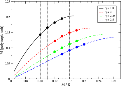
Figure 4: Single static neutron star models in the compactness - gravitational mass plane. The right end of each curve is the maximum mass model. The gravitational mass $M$ is rescaled by the polytropic constant $\kappa$: $\bar{M}=\kappa^{-1/(2(\gamma-1))}\,M$. The dots correspond to values of compactness considered in the present work.

Figure 5: Equatorial to polar ratio of the radial derivative of the enthalpy (cusp indicator) as a function of the orbital separation. Left (right) panel is for synchronized (irrotational) binary systems with the adiabatic index $\gamma=2.5$. Solid, dotted, dashed, and long-dashed curves denote the cases of compactness $M/R=0.14~{}{\rm vs}~{}0.14$, $0.16~{}{\rm vs}~{}0.16$, $0.18~{}{\rm vs}~{}0.18$, and $0.20~{}{\rm vs}~{}0.20$, respectively.

Figure 6: Same as Fig. 5 but for $\gamma=2.25$. Solid, dotted, dashed, and long-dashed curves denote the cases of compactness $M/R=0.12~{}{\rm vs}~{}0.12$, $0.14~{}{\rm vs}~{}0.14$, $0.16~{}{\rm vs}~{}0.16$, and $0.18~{}{\rm vs}~{}0.18$, respectively.

Figure 7: Same as Fig. 5 but for $\gamma=1.8$. Solid, dotted, dashed, and long-dashed curves denote the cases of compactness $M/R=0.08~{}{\rm vs}~{}0.08$, $0.10~{}{\rm vs}~{}0.10$, $0.12~{}{\rm vs}~{}0.12$, and $0.14~{}{\rm vs}~{}0.14$, respectively.

Figure 8: Same as Fig. 5 but for different-mass binary systems compared with an identical-mass binary system. The solid curve denotes the case of identical-mass binary system with compactness $M/R=0.16~{}{\rm vs}~{}0.16$. Thin and thick dashed curves are, respectively, for the more massive and less massive star of a different-mass binary system with $M/R=0.16~{}{\rm vs}~{}0.18$.

Figure 9: Same as Fig. 8 but for $\gamma=2.25$ The solid curve denotes the case of identical-mass binary system with compactness $M/R=0.14~{}{\rm vs}~{}0.14$. Thin and thick dashed curves are, respectively, for the more massive and less massive star of a different-mass binary system with $M/R=0.14~{}{\rm vs}~{}0.16$.

Figure 10: Same as Fig. 8 but for $\gamma=1.8$ The solid curve denotes the case of identical-mass binary system with compactness $M/R=0.10~{}{\rm vs}~{}0.10$. Thin and thick dashed curves are, respectively for the more massive and less massive star of a different-mass binary system with $M/R=0.10~{}{\rm vs}~{}0.12$.

Figure 11: Equatorial to polar ratio of the radial derivative of the enthalpy (cusp indicator) as a function of the orbital separation. Left (right) panel is for synchronized (irrotational) binary systems with the compactness $M/R=0.14~{}{\rm vs}~{}0.14$. Solid, dotted, dashed, and long-dashed curves denote the cases of adiabatic indices $\gamma=2.5$, 2.25, 2, and 1.8, respectively.

IV Numerical results

The spirit of the quasiequilibrium approach is to model the (gravitational-radiation driven) evolution of a neutron star binary by a sequence of steady-state circular-orbit configurations. Along the sequence the baryon number is kept constant, since no matter loss occurs during the evolution of each star, until the end of the inspiral stage. Such constant-baryon-number sequences are called evolutionary sequences.

We have computed numerous evolutionary sequences, for different values of the adiabatic index $\gamma$ and various compactness. We have used 5 (resp. 4) domains for each star and the space around it in the case of a large (resp. small) separation. In each domain, the number of collocation points of the spectral method is chosen to be $N_{r}\times N_{\theta}\times N_{\varphi}=25\times 17\times 16$ or $33\times 25\times 24$, where $N_{r}$, $N_{\theta}$, and $N_{\varphi}$ denote the number of collocation points in respectively the radial, polar, and azimuthal directions.

As in Paper III, we parametrize the difference in baryon mass between the two stars by the values of compactness of the stars like $[(M/R)_{\infty,\rm star~{}1}$ vs $(M/R)_{\infty,\rm star~{}2}]$, where $(M/R)_{\infty}$ denotes the compactness of the considered star at infinite separation or equivalently that of an isolated spherical star with the same baryon number. Hereafter, we abbreviate $(M/R)_{\infty,\rm star~{}1}$ vs $(M/R)_{\infty,\rm star~{}2}$ as $M/R$ for simplicity. According to recent nuclear equations of state, the compactness of a $M=1.4\,M_{\odot}$ neutron star is in the range $0.12\leq M/R\leq 0.20$, depending on the equation of state Haens03 . We therefore explore this range of compactness for our polytropic equations of state. We display the compactness parameters used for each adiabatic index $\gamma$ in Fig. 4. For each couple of values $(\gamma,M/R)$, one can see in Fig. 4 how far the considered model is from the maximum mass configuration.

Since we have already shown numerous results for $\gamma=2$ in Paper III, we focus here on results for $\gamma=2.5$, $2.25$, and $1.8$. We also consider the case $\gamma=3$ in Sec. V. However note that this value is too large for a realistic equation of state of neutron star.

IV.1 End points of the sequences

The start of mass exchange between the two stars marks the end of the existence of quasiequilibrium configurations. This mass-shedding corresponds to the appearance of a cusp at the surface of the lightest star (or both stars in the equal-mass case). This cusp reveals the vanishing of the gradient of enthalpy in the direction of the companion. Hence we consider the equatorial to polar ratio of the radial derivative of the enthalpy

$$\chi:={(\partial H/\partial r)_{\rm eq,comp}\over(\partial H/\partial r)_{\rm pole}}$$ (32)

as a dimensionless cusp indicator: $\chi=1$ at infinite separation, whereas $\chi=0$ when the cusp appears. The variation of $\chi$ along various evolutionary sequences is shown in Figs. 5 – 7 for identical-mass binary systems and in Figs. 8 – 10 for different-mass systems compared with identical-mass ones. The horizontal axis presents the orbital coordinate separation between the two coordinate centers (maxima of density), $d$, normalized by the summation of the coordinate radii of stars in the direction of their companions ($a_{1}$ and $a_{1}^{\prime}$):

$${\tilde{d}}:=\frac{d}{a_{1}+a_{1}^{\prime}}.$$ (33)

This dimensionless quantity is an indicator of the contact between the two stars: ${\tilde{d}}=1$ corresponds to the two stellar surfaces touching each other. Note here that $d$, $a_{1}$, and $a_{1}^{\prime}$ are all coordinate lengths, our coordinates being defined by the line element (5).

From Figs. 5 – 7, one can see that the lines seem to focus toward the point $d/(a_{1}+a_{1}^{\prime})=1$ and $\chi=0$ in the case of synchronized binary systems. This implies that synchronized binary systems of identical-mass stars in quasiequilibrium end their sequences by the contact between the two stars. It is worth to point out that the curves for all cases of compactness take almost the same tracks, but very slightly deviate from each other: the curves of larger compactness are located below those of smaller compactness. On the other hand, in the case of irrotational binary systems, the curves seem to reach $\chi=0$ at ${\tilde{d}}>1$. This means that the end point of quasiequilibrium sequences of irrotational binary systems is a detached configuration with a cusp point. Let us recall that in Paper II, we have found the same result in the Newtonian regime. This tendency is enhanced for the case of larger compactness. Note here that in Figs. 5 and 6, the curves with larger compactness in the case of irrotational binary systems turn slightly toward the vertical axis around $\chi\sim 0.5$. This comes from the numerical error.

The quasiequilibrium sequences should exist up to $\chi=0$. However, the multidomain spectral method we employ cannot handle cusp-like figures because in the surface-fitted coordinate procedure we assume that the stellar surface is smooth (see Sec. IV.E of Paper I for a detailed discussion of this point). Indeed our numerical scheme fails to converge when $\chi\rightarrow 0$. Monitoring the convergence by the relative difference $\delta H$ between the enthalpy fields of two successive computational steps, we hardly reach $\delta H<10^{-5}$ for synchronized binary systems when the orbital separation is such that $\chi\sim 0.4$. For irrotational configurations, although it is still possible to reach $\delta H\sim 10^{-6}$ when the orbital separation is such that $\chi\sim 0.4-0.5$, small but unphysical oscillations of the stellar surface appear. This results in the spurious (albeit slight) change of direction near the end of some curves in Figs. 5 and 6. These tendencies are enhanced for stiffer equation of state (larger values of $\gamma$) and more compact stars (larger values of $M/R$). Therefore, we stop the computations around $\chi\sim 0.4-0.5$.

We compare the evolution of the cusp indicator $\chi$ for different-mass binaries with that for identical-mass ones in Figs. 8 – 10. When extrapolating the curves toward $\chi=0$, the sequences seem to terminate by a cusp at the surface of the lightest star, both for synchronized and irrotational systems, while the heaviest star keeps its shape close to a spherical one. It is worth to note here that as soon as the two masses differ, even slightly, the sequence of a synchronized binary system terminates by a detached mass-shedding limit (Roche limit). Indeed the line for the less massive star is always located below that for identical-mass stars which reach $\chi=0$ at ${\tilde{d}}=1$. This implies that the line for the less massive star seems to always reach $\chi=0$ at ${\tilde{d}}>1$.

In Fig. 11, the evolution of $\chi$ is shown for a fixed value of the compactness parameter, $M/R=0.14~{}{\rm vs}~{}0.14$, and various values of the adiabatic index $\gamma$. It appears clearly that the curves of small $\gamma$ are located below those of large $\gamma$. This means that at fixed relative orbital separation ${\tilde{d}}$ and fixed compactness, a configuration with small $\gamma$ is closer to the mass-shedding limit than a configuration with large $\gamma$. The reason is that stars with small adiabatic index have centrally concentrated structures with some extended low density halos. Such low density outer layers result in a smaller $\chi$.

Figure 12: Relative change in central energy density as a function of the orbital separation between the centers of mass of each star. Left (right) panel is for synchronized (irrotational) binary systems with the adiabatic index $\gamma=2.5$. Solid, dotted, dashed, and long-dashed curves denote identical-mass binary systems with compactness $M/R=0.14~{}{\rm vs}~{}0.14$, 0.16 vs 0.16, 0.18 vs 0.18, and 0.20 vs 0.20, respectively.

Figure 13: Same as Fig. 12 but for $\gamma=2.25$. Solid, dotted, dashed, and long-dashed curves denote identical-mass binary systems with compactness $M/R=0.12~{}{\rm vs}~{}0.12$, 0.14 vs 0.14, 0.16 vs 0.16, and 0.18 vs 0.18, respectively.

Figure 14: Same as Fig. 12 but for $\gamma=1.8$ Solid, dotted, dashed, and long-dashed curves denote identical-mass binary systems with compactness $M/R=0.08~{}{\rm vs}~{}0.08$, 0.10 vs 0.10, 0.12 vs 0.12, and 0.14 vs 0.14, respectively.

Figure 15: Relative change in central energy density as a function of the cusp indicator $\chi$. Left (right) panel is for synchronized (irrotational) binary systems with the adiabatic index $\gamma=2.5$. Solid curves with open circle, square, diamond, and triangle denote identical-mass binary systems of compactness $M/R=0.14~{}{\rm vs}~{}0.14$, 0.16 vs 0.16, 0.18 vs 0.18, and 0.20 vs 0.20, respectively. Thick and thin dotted curves are for the less and more massive stars of the binary system with $M/R=0.14~{}{\rm vs}~{}0.16$, thick and thin dashed curves for those with $M/R=0.16~{}{\rm vs}~{}0.18$, and thick and thin long-dashed curves for those with $M/R=0.18~{}{\rm vs}~{}0.20$.

Figure 16: Same as Fig. 15 but for $\gamma=2.25$. Solid curves with open circle, square, diamond, and triangle denote identical-mass binary systems of compactness $M/R=0.12~{}{\rm vs}~{}0.12$, 0.14 vs 0.14, 0.16 vs 0.16, and 0.18 vs 0.18, respectively. Thick and thin dotted curves correspond respectively to the less and more massive stars of the binary system with $M/R=0.12~{}{\rm vs}~{}0.14$, thick and thin dashed curves for those with $M/R=0.14~{}{\rm vs}~{}0.16$, and thick and thin long-dashed curves for those with $M/R=0.16~{}{\rm vs}~{}0.18$.

Figure 17: Same as Fig. 15 but for $\gamma=1.8$. Solid curves with open circle, square, diamond, and triangle denote identical-mass binary systems of compactness $M/R=0.08~{}{\rm vs}~{}0.08$, 0.10 vs 0.10, 0.12 vs 0.12, and 0.14 vs 0.14, respectively. Thick and thin dotted curves are for the less and more massive stars of the binary system with $M/R=0.08~{}{\rm vs}~{}0.10$, thick and thin dashed curves for those with $M/R=0.10~{}{\rm vs}~{}0.12$, and thick and thin long-dashed curves for those with $M/R=0.12~{}{\rm vs}~{}0.14$.

Figure 18: Relative change in central energy density as a function of the cusp indicator $\chi$. Left (right) panel is for synchronized (irrotational) binary systems with compactness $M/R=0.14~{}{\rm vs}~{}0.14$. Solid, dotted, dashed, and long-dashed curves denote the cases of $\gamma=2.5$, 2.25, 2, and 1.8, respectively.

IV.2 Relative change in central density

Let us now examine the relative change in central energy density along an evolutionary sequence. In Figs. 12 – 14 in depicted the variation of the quantity

$$\delta e_{c}:={e_{c}-e_{c,\infty}\over e_{c,\infty}},$$ (34)

where $e_{c}$ and $e_{c,\infty}$ denote the central proper energy density of respectively the actual star and an isolated spherical star with the same baryon mass (or in other words, that at infinite separation). One can see from these figures that for all sequences the central energy density decreases as the orbit shrinks. It is also found that this decrease is larger for larger compactness, at fixed adiabatic index and rotation state. Note that the magnitude of the decrease is very different between the synchronized case and the irrotational one: $\sim 10\%$ for synchronized binaries versus a few $\%$ for irrotational ones.

The relative change in central energy density is presented as a function of the cusp indicator $\chi$ in Figs. 15 – 17, in order to evaluate the total change at the end of the sequence ($\chi=0$). It is found from these figures that the central energy density for large compactness decreases more than that for small compactness. Furthermore, we can see that the decreasing track of central energy density is determined by the compactness of the star itself and not by that of its companion, even though the value itself is affected by the companion star. This effect is clearly found for synchronized binary systems. For irrotational systems, since the amount of decrease is very small and the curves include some numerical errors, it is not clear whether the decrease depends only on the compactness of the star and not on that of its companion. However the same tendency could be found, in particular in the case of a soft equation of state like $\gamma=1.8$ (see Fig. 17). Note here that the slight changes of direction in the curves around $\chi\sim 0.5$ for large compactness in the irrotational case in Figs. 15 and 16 is due to the numerical error discussed in the previous subsection IV.1.

Although the sequences stop at around $\chi\simeq 0.4$, it is possible to predict how much the central energy density decreases at the mass-shedding limit by extrapolating the curves in Figs. 15 – 17. For instance, the central energy density of synchronized binary systems with $\gamma=2.25$ may decrease by 10 % – 15 % in the range of $M/R=0.12~{}{\rm vs}~{}0.12$ – 0.18 vs 0.18.

Figure 18 is shown in order to investigate the behavior of the relative change in central energy density when varying the adiabatic index and keeping the compactness fixed. It is found that the rate of decrease is lower for larger adiabatic indices. This is because the larger the adiabatic index, the closer the matter to the incompressible state in which the central energy density does not change.

Figure 19: ADM mass and total angular momentum of the binary system as a function of the orbital angular velocity. Top (bottom) panels are for identical-mass (different-mass) binary systems of compactness $M/R=0.16~{}{\rm vs}~{}0.16$ ($M/R=0.16~{}{\rm vs}~{}0.18$) with the adiabatic index $\gamma=2.5$. In each panel, the solid curve denotes the synchronized case, and the dashed one the irrotational one.

Figure 20: Same as Fig. 19 but for $\gamma=2.25$. Top (bottom) panels are for identical-mass (different-mass) binary systems of compactness $M/R=0.14~{}{\rm vs}~{}0.14$ ($M/R=0.14~{}{\rm vs}~{}0.16$).

Figure 21: Same as Fig. 19 but for $\gamma=1.8$. Top (bottom) panels are for identical-mass (different-mass) binary systems of compactness $M/R=0.10~{}{\rm vs}~{}0.10$ ($M/R=0.10~{}{\rm vs}~{}0.12$).

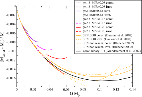
Figure 22: Relative binding energy along evolutionary sequences of equal-mass binary neutron stars, compared with (i) analytical results at the 3rd post-Newtonian order for point-masses by Damour et al. 2000 DamouJS00 , Damour et al. 2002 DamouGG02 and Blanchet 2002 Blanc02a , and with (ii) numerical results for corotating binary black holes by Grandclément et al. 2002 GrandGB02 . $\Omega$ is the orbital angular velocity and $M_{0}$ is twice the gravitational mass of a single static neutron star (resp. black hole) of the same baryon number (resp. same horizon area) as that defining the considered sequence.

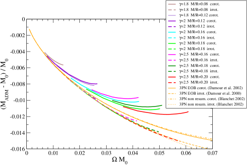
Figure 23: Enlargement of Fig. 22 in the neutron star region, with some additional sequences.

IV.3 ADM mass and total angular momentum

The variation of the ADM mass $M_{\rm ADM}$ and total angular momentum $J$ along an evolutionary sequence is presented in Figs. 19 – 21. These figures show that a turning point (minimum of $M_{\rm ADM}$ or $J$) appears for synchronized binaries with $\gamma=2.5$ and $2.25$. On the other hand, we cannot find it in the synchronized case with $\gamma=1.8$ and in any of irrotational sequences. Note that the position along the sequence of the turning point in the ADM mass and the total angular momentum coincide with each other, as expected from Eq. (31). The turning points are also found in the different-mass case for synchronized binary systems with $\gamma=2.5$ and 2.25. However, their position is closer to the end point of the sequence than that in the identical-mass case. Since, as mentioned above, we stop the computation slightly before the end point of quasiequilibrium sequences, there remains the possibility that the turning point may exist in the range $0<\chi<0.4$, even if we do not find it in the synchronized case with $\gamma=1.8$ and in the irrotational case. The complete discussion about the existence of the turning point for various adiabatic indices and compactness will be presented in Sec. V.

In Figs. 22 – 23, we present the ADM mass as a function of the orbital angular velocity, as in Figs. 19 – 21, but with a scaling defined by twice the gravitational mass of the single static neutron star of the same baryon number as that of the sequence, $M_{0}$ (whereas in Figs. 19 – 21, the scaling was set by the polytropic constant $\kappa$). Note that $M_{0}$ can also be viewed as the ADM mass at infinite separation. This enables us to compare with third order post-Newtonian results for point-mass particles obtained in the Effective One Body (EOB) approach by Damour et al. DamouJS00 ; DamouGG02 or in the standard non-resummed post-Newtonian framework by Blanchet Blanc02a . This also enables us to compare with corotating binary black holes, according to the numerical results by Grandclément et al. GrandGB02 . We note from these figures that the irrotational binary neutron star sequences are very close to the 3PN irrotational ones (dashed and dotted fine curves). Moreover, all curves converges at large separation (small value of $\Omega M_{0}$), which can be considered as a check of our numerical computations, especially the way $\Omega$ is determined (cf. Sec. IV.D.2 of Paper I).

Another interesting feature shown in Fig. 22 is the good agreement between the irrotational binary neutron star sequence with high compactness ($M/R=0.20$) and the binary black hole sequence. The latter is made of corotating black holes, but for $\Omega M_{0}\leq 0.06$, the spin effects are not very important, so that it is meaningful to compare the corotating black hole sequence up to $\Omega M_{0}\leq 0.06$ with the irrotational neutron star sequence. Finally, we notice from Fig. 23 that at a given compactness and separation, the configuration with smaller adiabatic index is more bound. Conversely, at a given adiabatic index and separation, the configuration with higher compactness is more bound.

Figure 24: Axial ratios $a_{2}/a_{1}$ (thick curves) or $a_{3}/a_{1}$ (thin curves) as a function of the cusp indicator $\chi$ along sequences with the adiabatic index $\gamma=2.5$. The left (right) panel is for synchronized (irrotational) binaries. Solid, dotted, dashed, and long-dashed curves correspond to $M/R=0.14~{}{\rm vs}~{}0.14$, 0.16 vs 0.16, 0.18 vs 0.18, and 0.20 vs 0.20, respectively.

Figure 25: Same as Fig. 24 but for $\gamma=2.25$. Solid, dotted, dashed, and long-dashed curves correspond to $M/R=0.12~{}{\rm vs}~{}0.12$, 0.14 vs 0.14, 0.16 vs 0.16, and 0.18 vs 0.18, respectively.

Figure 26: Same as Fig. 24 but for $\gamma=1.8$. Solid, dotted, dashed, and long-dashed curves correspond to $M/R=0.08~{}{\rm vs}~{}0.08$, 0.10 vs 0.10, 0.12 vs 0.12, and 0.14 vs 0.14, respectively.

Figure 27: Axial ratios as a function of the cusp indicator $\chi$. Left (right) is for synchronized (irrotational) binary systems with compactness $M/R=0.14~{}{\rm vs}~{}0.14$. Solid, dotted, dashed, and long-dashed curves correspond to the adiabatic indices $\gamma=2.5$, 2.25, 2, and 1.8, respectively. Thick and thin curves are respectively for the axial ratios $a_{2}/a_{1}$ and $a_{3}/a_{1}$.

IV.4 Deformation of the stars

The variation of the stellar shape along an evolutionary sequence is presented in Figs. 24 – 26. In these figures, we depict the (coordinate) axial ratio $a_{2}/a_{1}$ and $a_{3}/a_{1}$ as a function of the cusp indicator $\chi$. This allows one to speculate about the values of the axial ratios at the end point of the sequence, because the curves are close to straight lines. Since $\chi=0$ corresponds to the end point of the sequence (mass-shedding limit), we can evaluate the deformation of the stars at the end of the sequence by extrapolating the curves to $\chi=0$. The axial ratios at the end of the sequences are thus predicted to be $a_{2}/a_{1}\sim 0.7$ and $a_{3}/a_{1}\sim 0.6$ for synchronized binary systems with $\gamma=2.5$, and $a_{2}/a_{1}\sim 0.67-0.72$ and $a_{3}/a_{1}\sim 0.7-0.75$ for irrotational ones with $\gamma=2.5$. It is also possible to perceive that for the same value of $\chi$ the stars with larger compactness are closer to the spherical figure than those of smaller compactness.

We also present the change of the axial ratios along the sequence in Fig. 27 by fixing the compactness and varying the adiabatic index. It is clearly seen from this figure that that the deformation of the star is larger for larger adiabatic index.

IV.5 Contours of baryon density

Isocontours of the baryon density of various binary systems are shown in Figs. 28 – 30. There are two panels for different-mass binary systems in each figure. The left panel shows the result for the synchronized case while the right one is that for the irrotational case. In each panel, the left-hand side star is the less massive star. It is clearly seen that the lighter star is tidally deformed and elongated while the more massive star does not deviate very much from the spherical shape.

      

Figure 28: Isocontours of the baryon density for binary systems with the adiabatic index $\gamma=2.5$ and the compactness $M/R=0.16~{}{\rm vs}~{}0.18$. The left panel is for the synchronized case with the orbital separation $d_{G}/R_{\rm poly}=1.356$, while the right panel is for the irrotational one with $d_{G}/R_{\rm poly}=1.393$. The orbital axis is located on $x=0$ in each panel. The thick solid lines denote the surface of the stars.

      

Figure 29: Isocontours of the baryon density for binary systems with the adiabatic index $\gamma=2.25$ and the compactness $M/R=0.14~{}{\rm vs}~{}0.16$. The left panel is for the synchronized case with the orbital separation $d_{G}/R_{\rm poly}=1.765$, while the right panel is for the irrotational one with $d_{G}/R_{\rm poly}=1.775$. The orbital axis is located on $x=0$ in each panel.

      

Figure 30: Isocontours of the baryon density for binary systems with the adiabatic index $\gamma=1.8$ and the compactness $M/R=0.10~{}{\rm vs}~{}0.12$. The left panel is for the synchronized case with the orbital separation $d_{G}/R_{\rm poly}=4.391$, while the right panel is for the irrotational one with $d_{G}/R_{\rm poly}=4.257$. The orbital axis is located on $x=0$ in each panel.

IV.6 Tables of results

Finally, we summarize our numerical results about constant baryon number sequences in Tables 2 – 13. In each table, we first give the orbital separation defined as the distance $d_{G}$ between the two “center of mass” (see Eq. (128) of Paper I for a precise definition), in polytropic units:

$$\bar{d}_{G}:={d_{G}\over R_{\rm poly}},$$ (35)

where $R_{\rm poly}$ is the length constructed from the the polytropic constant $\kappa$ and the adiabatic index $\gamma$:

$$R_{\rm poly}:=\kappa^{1/2(\gamma-1)}.$$ (36)

We also list in Tables 2 – 13 the relative separation $\tilde{d}$ defined by Eq. (33) (let us recall that ${\tilde{d}}=1$ indicates the contact between the two stars). Next we give the dimensionless orbital angular velocity:

$$\bar{\Omega}:=\Omega\kappa^{1/2(\gamma-1)},$$ (37)

the dimensionless ADM mass:

$$\bar{M}:=M\kappa^{-1/2(\gamma-1)},$$ (38)

the dimensionless baryon mass:

$$\bar{M}_{\rm B}:=M_{\rm B}\kappa^{-1/2(\gamma-1)},$$ (39)

and the dimensionless total angular momentum:

$$\bar{J}:=J\kappa^{-1/(\gamma-1)}.$$ (40)

The absolute values of the relative errors in the virial theorem, $|VE(M)|$, $|VE(FUS)|$, and $|VE(GB)|$, are defined by Eqs. (28) – (30). $\delta e_{c}$ is the relative change in central energy density defined by Eq. (34). In the tables, primes denote values for the more massive star, and the symbol $\dagger$ denotes the turning point in the ADM mass (and the total angular momentum) along the sequence.

V Discussion

As shown by Friedman et al. FriedUS02 , the minimum (turning point) in the ADM mass in a constant baryon number sequence locates the appearance of a secular (resp. dynamical) instability for synchronized (resp. irrotational) binaries, thus defining the innermost stable circular orbit (ISCO). The frequency at the ISCO is a potentially observable parameter by the gravitational wave detectors, and thus a very interesting quantity. The position of the ISCO for identical-mass binary systems is depicted as a function of the compactness parameter in Fig. 31. In this figure, the Newtonian results are shown as $M/R=0$. The corresponding values of $\chi$ for the irrotational binaries are slightly different from those in Paper II. This is because we have improved our numerical code to decrease the aliasing error which appears in the spectral method CanutHQZ88 .

Several things can be found and predicted from Fig. 31. Firstly, the turning points are found for synchronized binary systems for $\gamma\geq 2$ and for irrotational ones for $\gamma\geq 2.5$. This last finding agrees with the results of Uryu et al. UryuSE00 . The turning point might exist for adiabatic index slightly lower than 2 for synchronized binary systems and 2.5 for irrotational ones. However, since it is very difficult for our numerical code to calculate quasiequilibrium figures of $\chi<0.4$ for mildly relativistic cases and $\chi<0.5$ for highly relativistic ones, we cannot determine the exact value of the minimum adiabatic index which has the turning point. Secondly, the quantity $\chi$ at the turning point increases proportionally to the compactness of the stars. This implies that the relative orbital separation at the turning point increases with the increase of the compactness. We should comment here that the tendency for the irrotational binary system with $\gamma=3$ was formerly given by Uryu et al. UryuSE00 . Thirdly, the inclination of lines for synchronized binary systems is larger than that for irrotational ones. Fourthly, we may assert that a turning point is found in Newtonian calculations for some value of the adiabatic index $\gamma$, it should exist in the general relativistic computations (within the IWM approximation) for the same value of $\gamma$, because the lines in Fig. 31 have a positive slope. It is worth to point out that even if the turning point is not found in the Newtonian sequences, the possibility to find it in the general relativistic computations does not vanish. In Fig. 31, some vertical lines which denote the maximum values of compactness for stable spherical stars are depicted. They show the limit of the existence of the turning point for each adiabatic index. Then, for a given adiabatic index, the turning point could exist from a compactness $M/R>0$ to the maximum $(M/R)_{\rm max}$ taking into account the fact that the line of the turning point has a positive inclination.

Figure 31: Positions of the turning points of the ADM mass (and total angular momentum) in the sequence as a function of the compactness parameter. Solid curve with filled circle is for the irrotational binary system with $\gamma=3$. Dotted with open square, dashed with open diamond, and long-dashed with open triangle denote the results of synchronized binary systems with $\gamma=2.5$, 2.25, and 2, respectively. Vertical solid, dotted, dashed, and long-dashed lines are maximum values of compactness for stable spherical stars (at $\chi=1$) for $\gamma=3$, 2.5, 2.25, 2, and 1.8, respectively.

VI Summary

We have developed a numerical code for computing quasiequilibrium sequences of binary neutron stars through the series of works GourGTMB01 ; TanigGB01 ; TanigG02a ; TanigG02b . In the present article, we have presented the results of relativistic computations of both synchronized and irrotational rotation states, for polytropic equations of state with several adiabatic indices. We have considered not only binary systems composed of identical-mass stars but also different-mass systems. We have investigated the behaviors of various physical quantities along constant baryon number sequences (evolutionary sequences): the relative change in central energy density, the ADM mass, the total angular momentum, the shape of the figures, as well as the location of the end point and that of the turning point in the ADM mass and angular momentum.

As one of interesting results, we propose, as a conjecture, that if the turning points defining the ISCO are found for the Newtonian calculations for some adiabatic index $\gamma$, they should exist in the general relativistic computations for the same value of $\gamma$. Of course, this conjecture is derived from the results of non-realistic cases such as synchronized binary systems or irrotational ones with $\gamma=3$. Furthermore, since the inclination of lines in Fig. 31 is positive, it is not possible to exactly predict whether or not a turning point appears in the IWM approximation when there is no turning point in the Newtonian calculation. However, if the computations of irrotational binary systems for $\chi<0.2$ could be obtained in the future with sufficient accuracy in Newtonian gravity, which is easier to be calculated than in the relativistic framework, it would be possible to speculate about the turning points in the IWM approximation without computations.

The numerical results presented in this article are freely available from http://www.lorene.obspm.fr/data/ This web page provides binary data files containing the whole binary neutron stars configurations as well as some codes to read them.

Table 1: Comparison with the results of Uryu, Shibata and Eriguchi UryuSE00 and Shibata and Uryu ShibaU01 ; Uryu03 .

	$M/R$	$\bar{M}_{\rm B}$	$0.5\times\bar{M}$	$M_{\rm B}\Omega$	$J/M_{\rm ADM}^{2}$	$d_{G}/M_{\rm ADM}$
$\gamma=2.5$
this work	0.14	0.08742	0.07974	0.01836	0.9563	8.815
Uryu et al.	0.14	0.0874	0.0797	0.0189	0.981	8.56
$\gamma=2.25$
this work	0.12	0.09316	0.08639	0.01414	1.004	10.42
Uryu et al.	0.12	0.0932	0.0864	0.0145	1.03	10.3
this work	0.14	0.1080	0.09886	0.01825	0.9521	8.812
Uryu et al.	0.14	0.108	0.0988	0.0189	0.975	8.52
$\gamma=2$
this work	0.12	0.1299	0.1211	0.01423	0.9972	10.42
Uryu et al.	0.12	0.130	0.121	0.0144	1.02	10.3
this work	0.14	0.1461	0.1347	0.01809	0.9474	8.805
Uryu et al.	0.14	0.146	0.135	0.0187	0.971	8.52
Shibata & Uryu	0.14	0.14614	0.1347	0.01885	0.9419	8.554
$\gamma=1.8$
this work	0.10	0.1725	0.1635	0.01038	1.065	12.88
Uryu et al.	0.10	0.173	0.164	0.0106	1.08	12.6
this work	0.12	0.1920	0.1803	0.01394	0.9947	10.49
Uryu et al.	0.12	0.192	0.180	0.0143	1.02	10.2
this work	0.14	0.2065	0.1924	0.01767	0.9456	8.871
Uryu et al.	0.14	0.207	0.192	0.0185	0.967	8.50

Table 2: Orbital angular velocity, ADM mass, total angular momentum, virial errors, axial ratios, relative change in central energy density, and the cusp indicator $\chi$ along constant baryon number sequences of identical mass binaries in synchronized motion, for various compactness. The symbol $\dagger$ denotes the turning point of the sequences.

Identical mass stars, Synchronized case, $\gamma=2.5$
$\bar{d}_{G}$	$\tilde{d}$	$\bar{\Omega}$	$\bar{M}$	$\bar{J}$	$|VE(M)|$	$|VE(GB)|$	$|VE(FUS)|$	$a_{2}/a_{1}$	$a_{3}/a_{1}$	$\delta e_{\rm c}$	$\chi$
$M/R=0.14~{}{\rm vs}~{}0.14,~{}~{}\bar{M}_{\rm B}=0.08742~{}{\rm vs.}~{}0.08742$
2.186	2.238	0.1126	0.1601	2.964(-2)	1.174(-5)	2.242(-5)	2.123(-5)	0.9689	0.9512	-1.397(-2)	0.8927
1.822	1.829	0.1452	0.1599	2.857(-2)	8.314(-6)	1.627(-5)	1.529(-5)	0.9443	0.9134	-2.447(-2)	0.8072
1.640	1.607	0.1681	0.1599	2.819(-2)	6.026(-6)	1.204(-5)	1.130(-5)	0.9187	0.8771	-3.453(-2)	0.7232
1.531	1.461	0.1851	0.1599	2.806(-2)	3.095(-5)	5.471(-5)	5.052(-5)	0.8924	0.8426	-4.397(-2)	0.6408
$\dagger$ 1.487	1.398	0.1928	0.1599	2.805(-2)	2.776(-5)	4.804(-5)	4.397(-5)	0.8774	0.8240	-4.897(-2)	0.5948
1.458	1.352	0.1983	0.1599	2.806(-2)	2.640(-2)	4.414(-5)	4.020(-5)	0.8650	0.8091	-5.288(-2)	0.5573
1.421	1.290	0.2056	0.1599	2.810(-2)	2.633(-5)	4.088(-5)	3.712(-5)	0.8454	0.7865	-5.864(-2)	0.4984
1.395	1.242	0.2111	0.1599	2.815(-2)	2.766(-5)	4.321(-5)	4.045(-5)	0.8274	0.7665	-6.343(-2)	0.4445
$M/R=0.16~{}{\rm vs}~{}0.16,~{}~{}\bar{M}_{\rm B}=0.1005~{}{\rm vs.}~{}0.1005$
2.004	2.127	0.1336	0.1816	3.579(-2)	1.736(-5)	3.375(-5)	3.200(-5)	0.9647	0.9435	-1.840(-2)	0.8729
1.822	1.916	0.1523	0.1815	3.519(-2)	1.450(-5)	2.846(-5)	2.689(-5)	0.9523	0.9238	-2.455(-2)	0.8279
1.640	1.694	0.1759	0.1814	3.471(-2)	1.155(-5)	2.198(-5)	2.063(-5)	0.9316	0.8930	-3.417(-2)	0.7564
1.495	1.500	0.1998	0.1814	3.450(-2)	5.189(-5)	9.531(-5)	8.895(-5)	0.9021	0.8527	-4.663(-2)	0.6603
$\dagger$ 1.453	1.439	0.2077	0.1814	3.449(-2)	4.664(-5)	8.490(-5)	7.876(-5)	0.8894	0.8364	-5.156(-2)	0.6204
1.422	1.392	0.2139	0.1814	3.450(-2)	4.221(-5)	7.586(-5)	6.990(-5)	0.8780	0.8222	-5.580(-2)	0.5849
1.367	1.300	0.2258	0.1814	3.457(-2)	3.944(-5)	6.632(-5)	6.120(-5)	0.8510	0.7903	-6.496(-2)	0.5026
1.349	1.265	0.2301	0.1814	3.462(-2)	4.404(-5)	6.957(-5)	6.392(-5)	0.8390	0.7767	-6.862(-2)	0.4663
$M/R=0.18~{}{\rm vs}~{}0.18,~{}~{}\bar{M}_{\rm B}=0.1131~{}{\rm vs.}~{}0.1131$
1.822	2.019	0.1582	0.2016	4.191(-2)	2.354(-5)	4.687(-5)	4.417(-5)	0.9599	0.9342	-2.481(-2)	0.8489
1.640	1.794	0.1824	0.2016	4.133(-2)	1.872(-5)	3.723(-5)	3.505(-5)	0.9434	0.9084	-3.410(-2)	0.7885
1.531	1.651	0.2000	0.2015	4.110(-2)	3.294(-5)	5.649(-5)	4.700(-5)	0.9277	0.8853	-4.231(-2)	0.7339
1.459	1.551	0.2135	0.2015	4.100(-2)	3.069(-5)	5.196(-5)	4.248(-5)	0.9129	0.8648	-4.958(-2)	0.6845
$\dagger$ 1.409	1.479	0.2235	0.2015	4.098(-2)	6.083(-5)	1.115(-4)	1.021(-4)	0.8999	0.8474	-5.568(-2)	0.6418
1.368	1.414	0.2327	0.2015	4.100(-2)	5.309(-5)	9.712(-5)	8.790(-5)	0.8858	0.8292	-6.189(-2)	0.5967
1.313	1.322	0.2458	0.2015	4.110(-2)	4.138(-5)	7.013(-5)	6.147(-5)	0.8605	0.7986	-7.200(-2)	0.5182
1.295	1.287	0.2505	0.2015	4.116(-2)	4.174(-5)	6.643(-5)	5.739(-5)	0.8493	0.7857	-7.606(-2)	0.4840
$M/R=0.20~{}{\rm vs}~{}0.20,~{}~{}\bar{M}_{\rm B}=0.1250~{}{\rm vs.}~{}0.1250$
1.822	2.140	0.1632	0.2200	4.847(-2)	3.860(-5)	7.632(-5)	7.280(-5)	0.9670	0.9442	-2.554(-2)	0.8694
1.568	1.814	0.1994	0.2199	4.760(-2)	5.257(-5)	9.409(-5)	8.084(-5)	0.9464	0.9110	-3.973(-2)	0.7906
1.459	1.665	0.2192	0.2198	4.737(-2)	4.707(-5)	8.401(-5)	7.058(-5)	0.9310	0.8878	-4.949(-2)	0.7350
1.422	1.613	0.2266	0.2198	4.733(-2)	4.499(-5)	8.008(-5)	6.666(-5)	0.9243	0.8780	-5.357(-2)	0.7113
$\dagger$ 1.366	1.530	0.2389	0.2198	4.729(-2)	4.199(-5)	7.341(-5)	5.976(-5)	0.9114	0.8600	-6.098(-2)	0.6674
1.313	1.448	0.2515	0.2198	4.733(-2)	7.023(-5)	1.310(-4)	1.182(-4)	0.8955	0.8389	-6.954(-2)	0.6149
1.259	1.355	0.2658	0.2199	4.745(-2)	6.260(-5)	1.099(-4)	9.640(-5)	0.8727	0.8102	-8.066(-2)	0.5419
1.229	1.299	0.2740	0.2199	4.756(-2)	6.800(-5)	1.030(-4)	9.569(-5)	0.8560	0.7904	-8.789(-2)	0.4901

Table 3: Same as Table 2 but for different mass binary systems. The prime denotes the values for the more massive star.

Different mass stars, Synchronized case, $\gamma=2.5$
$\bar{d}_{G}$	$\tilde{d}$	$\bar{\Omega}$	$\bar{M}$	$\bar{J}$	$|VE(M)|$	$|VE(GB)|$	$|VE(FUS)|$	$a_{2}/a_{1}$	$a_{3}/a_{1}$	$\delta e_{\rm c}$	$\chi$
								$a_{2}^{\prime}/a_{1}^{\prime}$	$a_{3}^{\prime}/a_{1}^{\prime}$	$\delta e_{\rm c}^{\prime}$	$\chi^{\prime}$
$M/R=0.14~{}{\rm vs}~{}0.16,~{}~{}\bar{M}_{\rm B}=0.08742~{}{\rm vs.}~{}0.1005$
2.004	2.080	0.1305	0.1708	3.224(-2)	1.331(-5)	2.585(-5)	2.443(-5)	0.9535	0.9300	-1.939(-2)	0.8452
								0.9691	0.9480	-1.740(-2)	0.8833
1.822	1.870	0.1489	0.1707	3.170(-2)	1.120(-5)	2.191(-5)	2.066(-5)	0.9365	0.9051	-2.617(-2)	0.7888
								0.9581	0.9300	-2.318(-2)	0.8419
1.640	1.647	0.1721	0.1707	3.127(-2)	8.836(-6)	1.663(-5)	1.558(-5)	0.9072	0.8651	-3.711(-2)	0.6960
								0.9398	0.9017	-3.217(-2)	0.7763
1.531	1.500	0.1894	0.1706	3.113(-2)	3.528(-5)	6.227(-5)	5.704(-5)	0.8768	0.8267	-4.752(-2)	0.6040
								0.9218	0.8758	-4.031(-2)	0.7148
$\dagger$ 1.482	1.429	0.1981	0.1706	3.111(-2)	3.086(-5)	5.309(-5)	4.804(-5)	0.8567	0.8027	-5.387(-2)	0.5443
								0.9105	0.8604	-4.506(-2)	0.6775
1.440	1.362	0.2062	0.1706	3.112(-2)	2.918(-5)	4.788(-5)	4.367(-5)	0.8337	0.7764	-6.056(-2)	0.4767
								0.8984	0.8445	-4.989(-2)	0.6383
1.421	1.330	0.2100	0.1707	3.114(-2)	3.091(-5)	4.906(-5)	4.524(-5)	0.8209	0.7624	-6.395(-2)	0.4396
								0.8921	0.8365	-5.228(-2)	0.6181
$M/R=0.16~{}{\rm vs}~{}0.18,~{}~{}\bar{M}_{\rm B}=0.1005~{}{\rm vs.}~{}0.1131$
2.004	2.179	0.1364	0.1917	3.904(-2)	2.247(-5)	4.390(-5)	4.177(-5)	0.9606	0.9393	-1.936(-2)	0.8634
								0.9732	0.9541	-1.793(-2)	0.8951
1.822	1.965	0.1554	0.1916	3.839(-2)	1.908(-5)	3.759(-5)	3.562(-5)	0.9468	0.9181	-2.585(-2)	0.8150
								0.9640	0.9385	-2.372(-2)	0.8588
1.640	1.740	0.1792	0.1915	3.787(-2)	1.493(-5)	2.948(-5)	2.783(-5)	0.9238	0.8859	-3.608(-2)	0.7380
								0.9491	0.9144	-3.256(-2)	0.8023
1.495	1.546	0.2032	0.1915	3.762(-2)	2.677(-5)	4.474(-5)	3.698(-5)	0.8908	0.8413	-4.943(-2)	0.6339
								0.9286	0.8838	-4.357(-2)	0.7295
$\dagger$ 1.437	1.461	0.2145	0.1915	3.760(-2)	5.030(-5)	9.113(-5)	8.363(-5)	0.8701	0.8156	-5.715(-2)	0.5705
								0.9165	0.8666	-4.967(-2)	0.6879
1.386	1.380	0.2253	0.1915	3.763(-2)	4.373(-5)	7.603(-5)	6.901(-5)	0.8447	0.7858	-6.571(-2)	0.4947
								0.9025	0.8479	-5.620(-2)	0.6415
1.356	1.329	0.2330	0.1915	3.768(-2)	4.533(-5)	7.403(-5)	6.775(-5)	0.8249	0.7637	-7.168(-2)	0.4364
								0.8924	0.8349	-6.062(-2)	0.6086
$M/R=0.18~{}{\rm vs}~{}0.20,~{}~{}\bar{M}_{\rm B}=0.1131~{}{\rm vs.}~{}0.1250$
1.822	2.077	0.1608	0.2108	4.506(-2)	2.951(-5)	5.847(-5)	5.549(-5)	0.9561	0.9304	-2.583(-2)	0.8400
								0.9699	0.9471	-2.465(-2)	0.8763
1.640	1.848	0.1852	0.2107	4.445(-2)	4.642(-5)	8.175(-5)	7.062(-5)	0.9381	0.9029	-3.555(-2)	0.7760
								0.9578	0.9268	-3.349(-2)	0.8282
1.459	1.604	0.2164	0.2107	4.407(-2)	3.889(-5)	6.799(-5)	5.682(-5)	0.9050	0.8567	-5.182(-2)	0.6657
								0.9366	0.8935	-4.770(-2)	0.7485
$\dagger$ 1.389	1.502	0.2308	0.2107	4.403(-2)	5.752(-5)	1.047(-4)	9.380(-5)	0.8838	0.8294	-6.127(-2)	0.5987
								0.9238	0.8747	-5.560(-2)	0.7027
1.349	1.440	0.2399	0.2107	4.405(-2)	5.591(-5)	9.670(-5)	8.621(-5)	0.8672	0.8091	-6.800(-2)	0.5479
								0.9142	0.8613	-6.114(-2)	0.6695
1.313	1.378	0.2487	0.2107	4.411(-2)	5.155(-5)	8.475(-5)	7.485(-5)	0.8476	0.7860	-7.556(-2)	0.4883
								0.9035	0.8468	-6.699(-2)	0.6332
1.295	1.345	0.2534	0.2107	4.415(-2)	5.715(-5)	8.631(-5)	7.711(-5)	0.8354	0.7722	-7.967(-2)	0.4522
								0.8971	0.8384	-7.031(-2)	0.6120

Table 4: Same as Table 2 but for irrotational binaries.

Identical mass stars, Irrotational case, $\gamma=2.5$
$\bar{d}_{G}$	$\tilde{d}$	$\bar{\Omega}$	$\bar{M}$	$\bar{J}$	$|VE(M)|$	$|VE(GB)|$	$|VE(FUS)|$	$a_{2}/a_{1}$	$a_{3}/a_{1}$	$\delta e_{\rm c}$	$\chi$
$M/R=0.14~{}{\rm vs}~{}0.14,~{}~{}\bar{M}_{\rm B}=0.08742~{}{\rm vs.}~{}0.08742$
2.185	2.266	0.1129	0.1600	2.765(-2)	1.044(-5)	1.994(-5)	1.865(-5)	0.9678	0.9729	-4.680(-4)	0.9344
1.821	1.865	0.1459	0.1598	2.599(-2)	6.162(-6)	1.208(-5)	1.095(-5)	0.9403	0.9474	-1.371(-3)	0.8693
1.565	1.552	0.1803	0.1596	2.487(-2)	1.366(-5)	2.090(-5)	1.565(-6)	0.8903	0.9018	-3.843(-3)	0.7422
1.491	1.446	0.1930	0.1595	2.458(-2)	2.819(-5)	5.056(-5)	4.520(-5)	0.8608	0.8751	-5.587(-3)	0.6573
1.454	1.383	0.1999	0.1595	2.445(-2)	2.273(-5)	4.210(-5)	3.612(-5)	0.8384	0.8548	-6.944(-3)	0.5839
1.436	1.346	0.2036	0.1595	2.439(-2)	1.021(-5)	2.298(-5)	1.561(-5)	0.8230	0.8407	-7.880(-3)	0.5286
1.417	1.302	0.2075	0.1595	2.434(-2)	1.346(-5)	1.706(-6)	1.353(-5)	0.8027	0.8219	-9.217(-3)	0.4548
1.406	1.272	0.2100	0.1595	2.432(-2)	4.416(-5)	3.417(-5)	5.155(-5)	0.7881	0.8079	-1.036(-2)	0.4062
$M/R=0.16~{}{\rm vs}~{}0.16,~{}~{}\bar{M}_{\rm B}=0.1005~{}{\rm vs.}~{}0.1005$
2.003	2.159	0.1341	0.1814	3.313(-2)	1.458(-5)	2.834(-5)	2.643(-5)	0.9630	0.9688	-7.015(-4)	0.9216
1.821	1.952	0.1531	0.1813	3.215(-2)	1.132(-5)	2.204(-5)	2.023(-5)	0.9489	0.9557	-1.217(-3)	0.8873
1.638	1.735	0.1770	0.1811	3.119(-2)	6.595(-6)	1.327(-5)	1.170(-5)	0.9244	0.9332	-2.361(-3)	0.8262
1.492	1.541	0.2014	0.1810	3.048(-2)	1.761(-5)	2.864(-5)	2.062(-5)	0.8868	0.8992	-4.562(-3)	0.7261
1.455	1.486	0.2085	0.1810	3.031(-2)	4.860(-5)	9.070(-5)	8.259(-5)	0.8719	0.8857	-5.510(-3)	0.6815
1.418	1.424	0.2161	0.1809	3.016(-2)	3.861(-5)	7.434(-5)	6.531(-5)	0.8512	0.8669	-6.816(-3)	0.6118
1.381	1.341	0.2242	0.1809	3.003(-2)	2.983(-5)	1.013(-5)	3.139(-5)	0.8160	0.8343	-9.212(-3)	0.4776
1.370	1.311	0.2268	0.1809	2.999(-2)	9.006(-5)	8.473(-5)	1.159(-4)	0.8023	0.8212	-1.048(-2)	0.4336
$M/R=0.18~{}{\rm vs}~{}0.18,~{}~{}\bar{M}_{\rm B}=0.1131~{}{\rm vs.}~{}0.1131$
2.003	2.268	0.1396	0.2015	3.957(-2)	2.342(-5)	4.589(-5)	4.303(-5)	0.9687	0.9744	-6.386(-4)	0.9336
1.638	1.836	0.1837	0.2012	3.738(-2)	1.217(-5)	2.452(-5)	2.199(-5)	0.9377	0.9457	-2.020(-3)	0.8558
1.529	1.695	0.2018	0.2011	3.676(-2)	2.773(-5)	4.855(-5)	3.709(-5)	0.9180	0.9278	-3.182(-3)	0.8051
1.456	1.595	0.2156	0.2010	3.636(-2)	2.364(-5)	4.107(-5)	2.932(-5)	0.8986	0.9103	-4.452(-3)	0.7522
1.382	1.480	0.2313	0.2009	3.601(-2)	5.059(-5)	9.859(-5)	8.570(-5)	0.8674	0.8821	-6.561(-3)	0.6514
1.345	1.395	0.2399	0.2009	3.583(-2)	6.626(-5)	6.451(-5)	9.658(-5)	0.8335	0.8505	-9.023(-3)	0.5141
1.327	1.347	0.2443	0.2009	3.574(-2)	2.324(-4)	2.930(-4)	3.523(-4)	0.8126	0.8305	-1.139(-2)	0.4510
1.308	1.298	0.2489	0.2008	3.565(-2)	4.501(-4)	5.946(-4)	6.889(-4)	0.7909	0.8094	-1.453(-2)	0.4008
$M/R=0.20~{}{\rm vs}~{}0.20,~{}~{}\bar{M}_{\rm B}=0.1250~{}{\rm vs.}~{}0.1250$
1.821	2.178	0.1642	0.2197	4.471(-2)	3.029(-5)	6.026(-5)	5.617(-5)	0.9650	0.9712	-9.649(-4)	0.9219
1.565	1.860	0.2011	0.2194	4.304(-2)	1.725(-5)	3.517(-5)	3.136(-5)	0.9407	0.9487	-2.287(-3)	0.8590
1.383	1.608	0.2372	0.2192	4.196(-2)	2.926(-5)	5.391(-5)	3.697(-5)	0.9005	0.9124	-5.184(-3)	0.7493
1.346	1.549	0.2458	0.2191	4.177(-2)	2.349(-5)	4.314(-5)	2.574(-5)	0.8855	0.8989	-6.292(-3)	0.6993
1.328	1.512	0.2504	0.2191	4.168(-2)	3.678(-5)	8.046(-5)	5.968(-5)	0.8733	0.8877	-7.089(-3)	0.6457
1.309	1.464	0.2548	0.2191	4.155(-2)	9.508(-5)	1.215(-4)	1.618(-4)	0.8540	0.8697	-8.684(-3)	0.5621
1.291	1.417	0.2593	0.2191	4.141(-2)	3.268(-4)	4.764(-4)	5.496(-4)	0.8347	0.8515	-1.113(-2)	0.5015
1.272	1.370	0.2640	0.2190	4.126(-2)	6.048(-4)	8.985(-4)	1.013(-3)	0.8157	0.8334	-1.426(-2)	0.4565

Table 5: Same as Table 4 but for different mass binary systems. The prime denotes the values for the more massive star.

Different mass stars, Irrotational case, $\gamma=2.5$
$\bar{d}_{G}$	$\tilde{d}$	$\bar{\Omega}$	$\bar{M}$	$\bar{J}$	$|VE(M)|$	$|VE(GB)|$	$|VE(FUS)|$	$a_{2}/a_{1}$	$a_{3}/a_{1}$	$\delta e_{\rm c}$	$\chi$
								$a_{2}^{\prime}/a_{1}^{\prime}$	$a_{3}^{\prime}/a_{1}^{\prime}$	$\delta e_{\rm c}^{\prime}$	$\chi^{\prime}$
$M/R=0.14~{}{\rm vs}~{}0.16,~{}~{}\bar{M}_{\rm B}=0.08742~{}{\rm vs.}~{}0.1005$
2.003	2.112	0.1309	0.1707	2.978(-2)	1.129(-5)	2.193(-5)	2.036(-5)	0.9509	0.9581	-1.012(-3)	0.8976
								0.9677	0.9725	-5.307(-4)	0.9307
1.821	1.906	0.1496	0.1705	2.888(-2)	8.442(-6)	1.665(-5)	1.521(-5)	0.9316	0.9402	-1.799(-3)	0.8516
								0.9553	0.9609	-9.288(-4)	0.9004
1.638	1.687	0.1732	0.1704	2.800(-2)	4.911(-6)	9.372(-6)	8.187(-6)	0.8967	0.9083	-3.597(-3)	0.7634
								0.9339	0.9411	-1.813(-3)	0.8466
1.528	1.540	0.1908	0.1703	2.751(-2)	1.560(-5)	2.468(-5)	1.816(-5)	0.8576	0.8730	-6.068(-3)	0.6577
								0.9116	0.9209	-2.942(-3)	0.7884
1.491	1.484	0.1974	0.1703	2.735(-2)	3.031(-5)	5.431(-5)	4.769(-5)	0.8372	0.8545	-7.402(-3)	0.5939
								0.9012	0.9115	-3.515(-3)	0.7598
1.455	1.420	0.2045	0.1702	2.721(-2)	1.747(-5)	3.441(-5)	2.640(-5)	0.8071	0.8270	-9.393(-3)	0.4892
								0.8881	0.8996	-4.267(-3)	0.7218
1.436	1.382	0.2082	0.1702	2.715(-2)	9.138(-7)	1.224(-5)	1.942(-5)	0.7863	0.8075	-1.095(-2)	0.4182
								0.8798	0.8922	-4.740(-3)	0.6966
$M/R=0.16~{}{\rm vs}~{}0.18,~{}~{}\bar{M}_{\rm B}=0.1005~{}{\rm vs.}~{}0.1131$
1.821	2.002	0.1562	0.1913	3.515(-2)	1.487(-5)	2.951(-5)	2.721(-5)	0.9428	0.9508	-1.527(-3)	0.8751
								0.9618	0.9673	-8.614(-4)	0.9142
1.638	1.782	0.1805	0.1912	3.413(-2)	9.770(-6)	1.956(-5)	1.748(-5)	0.9153	0.9256	-2.943(-3)	0.8067
								0.9442	0.9510	-1.622(-3)	0.8697
1.565	1.688	0.1921	0.1911	3.374(-2)	2.498(-5)	4.281(-5)	3.331(-5)	0.8976	0.9096	-4.048(-3)	0.7612
								0.9333	0.9411	-2.188(-3)	0.8416
1.492	1.588	0.2051	0.1910	3.336(-2)	2.221(-5)	3.699(-5)	2.737(-5)	0.8726	0.8870	-5.704(-3)	0.6917
								0.9187	0.9278	-3.017(-3)	0.8028
1.455	1.534	0.2122	0.1910	3.319(-2)	2.025(-5)	3.301(-5)	2.328(-5)	0.8548	0.8710	-6.916(-3)	0.6365
								0.9092	0.9192	-3.593(-3)	0.7766
1.419	1.471	0.2198	0.1910	3.302(-2)	3.680(-5)	7.472(-5)	6.303(-5)	0.8280	0.8465	-8.712(-3)	0.5381
								0.8974	0.9085	-4.332(-3)	0.7425
1.393	1.417	0.2254	0.1909	3.291(-2)	2.161(-5)	6.228(-6)	2.607(-5)	0.7996	0.8197	-1.111(-2)	0.4382
								0.8867	0.8988	-5.015(-3)	0.7090
$M/R=0.18~{}{\rm vs}~{}0.20,~{}~{}\bar{M}_{\rm B}=0.1131~{}{\rm vs.}~{}0.1250$
1.821	2.115	0.1617	0.2106	4.146(-2)	2.407(-5)	4.781(-5)	4.445(-5)	0.9530	0.9605	-1.310(-3)	0.8967
								0.9682	0.9735	-7.934(-4)	0.9281
1.565	1.798	0.1984	0.2103	3.987(-2)	3.436(-5)	6.119(-5)	4.780(-5)	0.9182	0.9287	-3.278(-3)	0.8090
								0.9456	0.9527	-1.931(-3)	0.8699
1.492	1.701	0.2115	0.2102	3.945(-2)	3.030(-5)	5.434(-5)	4.047(-5)	0.9003	0.9124	-4.498(-3)	0.7614
								0.9345	0.9426	-2.605(-3)	0.8405
1.419	1.596	0.2263	0.2101	3.904(-2)	2.503(-5)	4.469(-5)	3.043(-5)	0.8736	0.8884	-6.432(-3)	0.6828
								0.9191	0.9287	-3.631(-3)	0.7987
1.382	1.534	0.2343	0.2101	3.886(-2)	1.287(-5)	2.740(-5)	1.110(-5)	0.8507	0.8675	-8.001(-3)	0.5961
								0.9089	0.9194	-4.359(-3)	0.7693
1.364	1.497	0.2386	0.2100	3.876(-2)	1.977(-5)	1.155(-5)	3.520(-5)	0.8320	0.8501	-9.495(-3)	0.5208
								0.9026	0.9138	-4.810(-3)	0.7503
1.346	1.457	0.2429	0.2100	3.866(-2)	1.021(-4)	1.261(-4)	1.631(-4)	0.8119	0.8309	-1.178(-2)	0.4581
								0.8951	0.9070	-5.342(-3)	0.7258

Table 6: Same as Table 2 but for $\gamma=2.25$.

Identical mass stars, Synchronized case, $\gamma=2.25$
$\bar{d}_{G}$	$\tilde{d}$	$\bar{\Omega}$	$\bar{M}$	$\bar{J}$	$|VE(M)|$	$|VE(GB)|$	$|VE(FUS)|$	$a_{2}/a_{1}$	$a_{3}/a_{1}$	$\delta e_{\rm c}$	$\chi$
$M/R=0.12~{}{\rm vs}~{}0.12,~{}~{}\bar{M}_{\rm B}=0.09316~{}{\rm vs.}~{}0.09316$
2.925	2.304	0.07708	0.1734	3.724(-2)	8.099(-6)	1.407(-5)	1.317(-5)	0.9726	0.9578	-1.402(-2)	0.9002
2.701	2.113	0.08635	0.1733	3.646(-2)	7.249(-6)	1.259(-5)	1.174(-5)	0.9649	0.9457	-1.787(-2)	0.8712
2.251	1.714	0.1117	0.1732	3.510(-2)	4.990(-6)	8.736(-6)	8.072(-6)	0.9354	0.9019	-3.171(-2)	0.7650
2.026	1.492	0.1296	0.1731	3.462(-2)	2.062(-5)	3.400(-5)	3.093(-5)	0.9027	0.8580	-4.536(-2)	0.6549
1.936	1.392	0.1383	0.1731	3.452(-2)	1.853(-5)	2.870(-5)	2.572(-5)	0.8808	0.8307	-5.355(-2)	0.5840
$\dagger$ 1.881	1.327	0.1440	0.1731	3.450(-2)	1.659(-5)	2.505(-5)	2.232(-5)	0.8626	0.8091	-5.978(-2)	0.5263
1.845	1.278	0.1481	0.1731	3.451(-2)	1.695(-5)	2.373(-5)	2.153(-5)	0.8471	0.7912	-6.468(-2)	0.4773
1.813	1.231	0.1519	0.1731	3.455(-2)	1.961(-5)	2.624(-5)	2.560(-5)	0.8297	0.7721	-6.961(-2)	0.4231
$M/R=0.14~{}{\rm vs}~{}0.14,~{}~{}\bar{M}_{\rm B}=0.1080~{}{\rm vs.}~{}0.1080$
2.701	2.229	0.09129	0.1985	4.535(-2)	1.297(-5)	2.327(-5)	2.192(-5)	0.9704	0.9535	-1.770(-2)	0.8879
2.251	1.821	0.1177	0.1983	4.366(-2)	9.395(-6)	1.688(-5)	1.573(-5)	0.9468	0.9171	-3.086(-2)	0.7986
2.026	1.600	0.1362	0.1982	4.302(-2)	7.380(-6)	1.267(-5)	1.170(-5)	0.9222	0.8820	-4.332(-2)	0.7109
1.936	1.505	0.1451	0.1982	4.285(-2)	3.392(-5)	5.874(-5)	5.399(-5)	0.9067	0.8611	-5.055(-2)	0.6580
1.846	1.402	0.1551	0.1982	4.275(-2)	2.858(-5)	4.793(-5)	4.339(-5)	0.8849	0.8336	-5.987(-2)	0.5862
$\dagger$ 1.808	1.354	0.1597	0.1982	4.274(-2)	2.765(-5)	4.403(-5)	3.958(-5)	0.8726	0.8186	-6.473(-2)	0.5464
1.756	1.284	0.1663	0.1982	4.277(-2)	2.930(-5)	4.107(-5)	3.686(-5)	0.8511	0.7936	-7.250(-2)	0.4779
1.724	1.235	0.1707	0.1982	4.283(-2)	3.209(-5)	4.785(-5)	4.456(-5)	0.8335	0.7740	-7.811(-2)	0.4228
$M/R=0.16~{}{\rm vs}~{}0.16,~{}~{}\bar{M}_{\rm B}=0.1219~{}{\rm vs.}~{}0.1219$
2.701	2.364	0.09540	0.2215	5.416(-2)	2.248(-5)	4.136(-5)	3.929(-5)	0.9754	0.9609	-1.775(-2)	0.9039
2.251	1.943	0.1227	0.2213	5.214(-2)	1.703(-5)	3.126(-5)	2.936(-5)	0.9569	0.9309	-3.044(-2)	0.8295
2.026	1.720	0.1417	0.2211	5.134(-2)	1.374(-5)	2.462(-5)	2.291(-5)	0.9384	0.9029	-4.208(-2)	0.7592
1.936	1.625	0.1507	0.2211	5.110(-2)	2.577(-5)	4.027(-5)	3.303(-5)	0.9271	0.8867	-4.864(-2)	0.7185
1.801	1.474	0.1663	0.2211	5.086(-2)	5.052(-5)	9.016(-5)	8.315(-5)	0.9027	0.8536	-6.189(-2)	0.6334
$\dagger$ 1.736	1.394	0.1749	0.2211	5.082(-2)	4.393(-5)	7.597(-5)	6.912(-5)	0.8851	0.8313	-7.040(-2)	0.5746
1.666	1.298	0.1850	0.2211	5.088(-2)	4.497(-5)	6.625(-5)	5.946(-5)	0.8582	0.7992	-8.194(-2)	0.4876
1.630	1.241	0.1906	0.2211	5.097(-2)	5.881(-5)	8.377(-5)	7.738(-5)	0.8384	0.7769	-8.920(-2)	0.4250
$M/R=0.18~{}{\rm vs}~{}0.18,~{}~{}\bar{M}_{\rm B}=0.1347~{}{\rm vs.}~{}0.1347$
2.701	2.522	0.09878	0.2419	6.251(-2)	3.691(-5)	6.915(-5)	6.619(-5)	0.9800	0.9677	-1.825(-2)	0.9190
2.251	2.084	0.1267	0.2416	6.018(-2)	2.898(-5)	5.451(-5)	5.162(-5)	0.9656	0.9434	-3.085(-2)	0.8576
2.026	1.854	0.1461	0.2415	5.922(-2)	2.451(-5)	4.556(-5)	4.254(-5)	0.9517	0.9211	-4.208(-2)	0.8011
1.891	1.709	0.1603	0.2414	5.878(-2)	3.901(-5)	6.457(-5)	5.406(-5)	0.9386	0.9011	-5.190(-2)	0.7505
1.712	1.502	0.1832	0.2414	5.842(-2)	7.229(-5)	1.321(-4)	1.219(-4)	0.9098	0.8605	-7.132(-2)	0.6458
$\dagger$ 1.662	1.439	0.1904	0.2414	5.839(-2)	6.523(-5)	1.173(-4)	1.074(-4)	0.8975	0.8445	-7.864(-2)	0.6036
1.577	1.320	0.2043	0.2414	5.849(-2)	5.633(-5)	9.448(-5)	8.565(-5)	0.8673	0.8072	-9.472(-2)	0.5033
1.554	1.284	0.2082	0.2414	5.855(-2)	6.519(-5)	1.036(-4)	9.563(-5)	0.8562	0.7943	-9.980(-2)	0.4677

Table 7: Same as Table 6 but for different mass binary systems. The prime denotes the values for the more massive star.

Different mass stars, Synchronized case, $\gamma=2.25$
$\bar{d}_{G}$	$\tilde{d}$	$\bar{\Omega}$	$\bar{M}$	$\bar{J}$	$|VE(M)|$	$|VE(GB)|$	$|VE(FUS)|$	$a_{2}/a_{1}$	$a_{3}/a_{1}$	$\delta e_{\rm c}$	$\chi$
								$a_{2}^{\prime}/a_{1}^{\prime}$	$a_{3}^{\prime}/a_{1}^{\prime}$	$\delta e_{\rm c}^{\prime}$	$\chi^{\prime}$
$M/R=0.12~{}{\rm vs}~{}0.14,~{}~{}\bar{M}_{\rm B}=0.09316~{}{\rm vs.}~{}0.1080$
2.701	2.169	0.08889	0.1859	4.063(-2)	9.821(-6)	1.738(-5)	1.630(-5)	0.9595	0.9400	-1.916(-2)	0.8577
								0.9744	0.9576	-1.665(-2)	0.8980
2.476	1.970	0.1005	0.1858	3.983(-2)	8.511(-6)	1.508(-5)	1.407(-5)	0.9464	0.9208	-2.513(-2)	0.8113
								0.9663	0.9443	-2.161(-2)	0.8655
2.251	1.763	0.1148	0.1858	3.912(-2)	7.046(-6)	1.249(-5)	1.160(-5)	0.9254	0.8914	-3.421(-2)	0.7396
								0.9538	0.9245	-2.894(-2)	0.8167
2.026	1.539	0.1330	0.1857	3.858(-2)	1.413(-5)	1.996(-5)	1.610(-5)	0.8872	0.8419	-4.929(-2)	0.6154
								0.9322	0.8925	-4.051(-2)	0.7370
1.936	1.440	0.1418	0.1857	3.845(-2)	2.219(-5)	3.581(-5)	3.212(-5)	0.8610	0.8105	-5.851(-2)	0.5336
								0.9187	0.8737	-4.719(-2)	0.6889
1.891	1.385	0.1466	0.1857	3.842(-2)	2.220(-5)	3.382(-5)	3.011(-5)	0.8430	0.7899	-6.427(-2)	0.4782
								0.9100	0.8621	-5.120(-2)	0.6590
$\dagger$ 1.866	1.353	0.1494	0.1857	3.841(-2)	2.148(-5)	3.200(-5)	2.882(-5)	0.8308	0.7763	-6.788(-2)	0.4410
								0.9045	0.8549	-5.365(-2)	0.6401
$M/R=0.14~{}{\rm vs}~{}0.16,~{}~{}\bar{M}_{\rm B}=0.1080~{}{\rm vs.}~{}0.1219$
2.476	2.090	0.1054	0.2099	4.857(-2)	1.519(-5)	2.769(-5)	2.606(-5)	0.9564	0.9340	-2.429(-2)	0.8402
								0.9716	0.9524	-2.183(-2)	0.8829
2.251	1.879	0.1203	0.2098	4.769(-2)	1.287(-5)	2.347(-5)	2.200(-5)	0.9404	0.9103	-3.265(-2)	0.7821
								0.9615	0.9358	-2.899(-2)	0.8415
2.026	1.655	0.1390	0.2097	4.698(-2)	9.989(-6)	1.804(-5)	1.681(-5)	0.9128	0.8721	-4.600(-2)	0.6867
								0.9449	0.9097	-4.003(-2)	0.7761
1.891	1.509	0.1529	0.2097	4.671(-2)	4.124(-5)	7.177(-5)	6.596(-5)	0.8840	0.8353	-5.852(-2)	0.5926
								0.9285	0.8858	-4.988(-2)	0.7155
1.846	1.457	0.1580	0.2097	4.665(-2)	3.974(-5)	6.562(-5)	5.982(-5)	0.8704	0.8188	-6.391(-2)	0.5494
								0.9212	0.8756	-5.397(-2)	0.6893
$\dagger$ 1.790	1.386	0.1649	0.2097	4.662(-2)	4.089(-5)	5.949(-5)	5.379(-5)	0.8485	0.7932	-7.193(-2)	0.4807
								0.9101	0.8606	-5.989(-2)	0.6502
1.765	1.353	0.1682	0.2097	4.662(-2)	3.651(-5)	5.655(-5)	5.304(-5)	0.8361	0.7793	-7.610(-2)	0.4425
								0.9043	0.8530	-6.290(-2)	0.6300
$M/R=0.16~{}{\rm vs}~{}0.18,~{}~{}\bar{M}_{\rm B}=0.1219~{}{\rm vs.}~{}0.1347$
2.251	2.010	0.1248	0.2314	5.600(-2)	2.279(-5)	4.251(-5)	4.018(-5)	0.9528	0.9266	-3.174(-2)	0.8189
								0.9687	0.9465	-2.973(-2)	0.8655
2.026	1.783	0.1440	0.2313	5.514(-2)	3.483(-5)	5.659(-5)	4.793(-5)	0.9324	0.8966	-4.399(-2)	0.7440
								0.9558	0.9253	-4.055(-2)	0.8120
1.891	1.638	0.1580	0.2313	5.474(-2)	3.189(-5)	5.143(-5)	4.267(-5)	0.9126	0.8693	-5.496(-2)	0.6747
								0.9437	0.9065	-4.995(-2)	0.7641
1.801	1.536	0.1687	0.2312	5.456(-2)	3.025(-5)	4.807(-5)	3.943(-5)	0.8933	0.8441	-6.480(-2)	0.6098
								0.9325	0.8899	-5.812(-2)	0.7212
$\dagger$ 1.709	1.421	0.1811	0.2312	5.448(-2)	4.422(-5)	7.306(-5)	6.528(-5)	0.8638	0.8081	-7.820(-2)	0.5146
								0.9165	0.8674	-6.886(-2)	0.6626
1.689	1.394	0.1840	0.2312	5.449(-2)	4.380(-5)	7.051(-5)	6.284(-5)	0.8551	0.7980	-8.179(-2)	0.4871
								0.9121	0.8614	-7.165(-2)	0.6468
1.666	1.362	0.1874	0.2312	5.450(-2)	4.438(-5)	6.860(-5)	6.099(-5)	0.8440	0.7852	-8.614(-2)	0.4523
								0.9067	0.8542	-7.496(-2)	0.6277

Table 8: Same as Table 6 but for irrotational binaries.

Identical mass stars, Irrotational case, $\gamma=2.25$
$\bar{d}_{G}$	$\tilde{d}$	$\bar{\Omega}$	$\bar{M}$	$\bar{J}$	$|VE(M)|$	$|VE(GB)|$	$|VE(FUS)|$	$a_{2}/a_{1}$	$a_{3}/a_{1}$	$\delta e_{\rm c}$	$\chi$
$M/R=0.12~{}{\rm vs}~{}0.12,~{}~{}\bar{M}_{\rm B}=0.09316~{}{\rm vs.}~{}0.09316$
2.924	2.331	0.07722	0.1733	3.503(-2)	7.443(-6)	1.278(-5)	1.184(-5)	0.9720	0.9764	-3.975(-4)	0.9392
2.699	2.145	0.08654	0.1732	3.399(-2)	6.429(-6)	1.096(-6)	1.004(-5)	0.9639	0.9689	-6.208(-4)	0.9189
2.249	1.756	0.1121	0.1730	3.186(-2)	3.645(-6)	5.956(-6)	5.181(-6)	0.9318	0.9390	-1.880(-3)	0.8364
2.023	1.540	0.1302	0.1729	3.081(-2)	1.034(-5)	1.390(-5)	1.027(-5)	0.8949	0.9051	-3.891(-3)	0.7350
1.933	1.440	0.1390	0.1728	3.041(-2)	1.791(-5)	2.913(-5)	2.545(-5)	0.8689	0.8813	-5.503(-3)	0.6559
1.887	1.384	0.1438	0.1728	3.023(-2)	1.578(-5)	2.575(-5)	2.189(-5)	0.8500	0.8640	-6.695(-3)	0.5929
1.842	1.315	0.1490	0.1728	3.006(-2)	8.452(-6)	1.842(-5)	1.320(-5)	0.8223	0.8385	-8.430(-3)	0.4915
1.818	1.272	0.1518	0.1728	2.998(-2)	7.529(-6)	4.168(-6)	4.072(-6)	0.8017	0.8194	-9.802(-3)	0.4169
$M/R=0.14~{}{\rm vs}~{}0.14,~{}~{}\bar{M}_{\rm B}=0.1080~{}{\rm vs.}~{}0.1080$
2.699	2.260	0.09153	0.1984	4.244(-2)	1.166(-5)	2.069(-5)	1.923(-5)	0.9696	0.9746	-5.469(-4)	0.9320
2.249	1.863	0.1182	0.1981	3.989(-2)	7.237(-6)	1.255(-5)	1.123(-5)	0.9440	0.9507	-1.557(-3)	0.8653
1.933	1.555	0.1460	0.1979	3.813(-2)	1.479(-5)	2.111(-5)	1.534(-5)	0.8979	0.9084	-4.220(-3)	0.7377
1.843	1.451	0.1562	0.1978	3.767(-2)	2.958(-5)	5.118(-5)	4.526(-5)	0.8710	0.8838	-6.024(-3)	0.6533
1.797	1.390	0.1617	0.1978	3.745(-2)	2.347(-5)	4.246(-5)	3.576(-5)	0.8502	0.8647	-7.406(-3)	0.5789
1.774	1.353	0.1647	0.1977	3.735(-2)	1.372(-5)	3.164(-5)	2.314(-5)	0.8352	0.8509	-8.379(-3)	0.5209
1.752	1.309	0.1677	0.1977	3.726(-2)	1.877(-5)	2.257(-6)	1.639(-5)	0.8148	0.8320	-9.855(-3)	0.4447
1.742	1.289	0.1690	0.1977	3.722(-2)	4.311(-5)	2.740(-5)	4.625(-5)	0.8052	0.8229	-1.068(-2)	0.4127
$M/R=0.16~{}{\rm vs}~{}0.16,~{}~{}\bar{M}_{\rm B}=0.1219~{}{\rm vs.}~{}0.1219$
2.699	2.396	0.09567	0.2213	5.089(-2)	1.986(-5)	3.624(-5)	3.404(-5)	0.9749	0.9799	-4.866(-4)	0.9442
2.249	1.985	0.1232	0.2210	4.795(-2)	1.381(-5)	2.503(-5)	2.292(-5)	0.9548	0.9611	-1.302(-3)	0.8911
2.024	1.769	0.1425	0.2208	4.649(-2)	9.182(-6)	1.624(-5)	1.431(-5)	0.9339	0.9418	-2.449(-3)	0.8342
1.934	1.677	0.1518	0.2207	4.592(-2)	2.305(-5)	3.618(-5)	2.759(-5)	0.9208	0.9297	-3.308(-3)	0.7978
1.843	1.580	0.1620	0.2206	4.536(-2)	2.066(-5)	3.166(-5)	2.288(-5)	0.9030	0.9134	-4.559(-3)	0.7458
1.753	1.472	0.1737	0.2206	4.483(-2)	4.918(-5)	8.947(-5)	8.036(-5)	0.8757	0.8885	-6.554(-3)	0.6574
1.707	1.404	0.1800	0.2205	4.459(-2)	2.734(-5)	5.954(-5)	4.726(-5)	0.8515	0.8664	-8.228(-3)	0.5623
1.662	1.307	0.1868	0.2205	4.434(-2)	1.526(-4)	1.638(-4)	2.070(-4)	0.8080	0.8257	-1.237(-2)	0.4113
$M/R=0.18~{}{\rm vs}~{}0.18,~{}~{}\bar{M}_{\rm B}=0.1347~{}{\rm vs.}~{}0.1347$
2.699	2.554	0.09906	0.2417	5.897(-2)	3.207(-5)	5.974(-5)	5.656(-5)	0.9798	0.9846	-4.427(-4)	0.9555
2.249	2.126	0.1274	0.2413	5.570(-2)	2.405(-5)	4.480(-5)	4.156(-5)	0.9643	0.9702	-1.115(-3)	0.9137
1.889	1.765	0.1614	0.2410	5.310(-2)	1.304(-5)	2.334(-5)	2.046(-5)	0.9337	0.9419	-3.042(-3)	0.8284
1.708	1.562	0.1849	0.2408	5.189(-2)	2.551(-5)	4.151(-5)	2.837(-5)	0.8982	0.9095	-5.944(-3)	0.7225
1.663	1.502	0.1918	0.2407	5.161(-2)	5.802(-5)	1.087(-4)	9.491(-5)	0.8826	0.8952	-7.211(-3)	0.6665
1.640	1.467	0.1953	0.2407	5.147(-2)	4.481(-5)	8.930(-5)	7.347(-5)	0.8704	0.8841	-8.092(-3)	0.6150
1.618	1.420	0.1989	0.2407	5.132(-2)	4.391(-5)	3.902(-5)	6.787(-5)	0.8509	0.8661	-9.735(-3)	0.5322
1.595	1.369	0.2026	0.2406	5.113(-2)	2.193(-4)	2.871(-4)	3.426(-4)	0.8288	0.8456	-1.248(-2)	0.4615

Table 9: Same as Table 8 but for different mass binary systems. The prime denotes the values for the more massive star.

Different mass stars, Irrotational case, $\gamma=2.25$
$\bar{d}_{G}$	$\tilde{d}$	$\bar{\Omega}$	$\bar{M}$	$\bar{J}$	$|VE(M)|$	$|VE(GB)|$	$|VE(FUS)|$	$a_{2}/a_{1}$	$a_{3}/a_{1}$	$\delta e_{\rm c}$	$\chi$
								$a_{2}^{\prime}/a_{1}^{\prime}$	$a_{3}^{\prime}/a_{1}^{\prime}$	$\delta e_{\rm c}^{\prime}$	$\chi^{\prime}$
$M/R=0.12~{}{\rm vs}~{}0.14,~{}~{}\bar{M}_{\rm B}=0.09316~{}{\rm vs.}~{}0.1080$
2.699	2.200	0.08910	0.1858	3.794(-2)	8.995(-6)	1.576(-5)	1.458(-5)	0.9582	0.9643	-8.350(-4)	0.9072
								0.9737	0.9778	-4.042(-4)	0.9404
2.474	2.006	0.1008	0.1857	3.678(-2)	7.210(-6)	1.246(-5)	1.134(-5)	0.9440	0.9512	-1.386(-3)	0.8716
								0.9651	0.9697	-6.597(-4)	0.9182
2.249	1.805	0.1152	0.1856	3.561(-2)	5.310(-6)	8.974(-6)	7.943(-6)	0.9210	0.9298	-2.511(-3)	0.8119
								0.9515	0.9570	-1.166(-3)	0.8822
2.023	1.587	0.1337	0.1854	3.447(-2)	1.322(-5)	1.850(-5)	1.394(-5)	0.8772	0.8896	-5.215(-3)	0.6903
								0.9273	0.9346	-2.322(-3)	0.8165
1.933	1.487	0.1427	0.1854	3.403(-2)	2.179(-5)	3.612(-5)	3.144(-5)	0.8447	0.8598	-7.435(-3)	0.5874
								0.9117	0.9203	-3.193(-3)	0.7718
1.887	1.429	0.1476	0.1853	3.382(-2)	1.794(-5)	3.037(-5)	2.523(-5)	0.8190	0.8363	-9.171(-3)	0.4967
								0.9014	0.9108	-3.804(-3)	0.7411
1.865	1.395	0.1501	0.1853	3.373(-2)	1.079(-5)	2.103(-5)	1.498(-5)	0.8010	0.8196	-1.042(-2)	0.4320
								0.8953	0.9052	-4.177(-3)	0.7220
$M/R=0.14~{}{\rm vs}~{}0.16,~{}~{}\bar{M}_{\rm B}=0.1080~{}{\rm vs.}~{}0.1219$
2.474	2.126	0.1058	0.2097	4.508(-2)	1.322(-5)	2.378(-5)	2.199(-5)	0.9546	0.9613	-1.128(-3)	0.8959
								0.9707	0.9753	-5.989(-4)	0.9314
2.249	1.921	0.1208	0.2096	4.371(-2)	1.029(-5)	1.834(-5)	1.665(-5)	0.9370	0.9449	-1.971(-3)	0.8498
								0.9598	0.9651	-1.026(-3)	0.9020
2.024	1.704	0.1398	0.2094	4.235(-2)	6.653(-6)	1.100(-5)	9.575(-6)	0.9055	0.9158	-3.843(-3)	0.7620
								0.9411	0.9477	-1.950(-3)	0.8509
1.888	1.560	0.1539	0.2093	4.156(-2)	1.779(-5)	2.613(-5)	1.900(-5)	0.8706	0.8841	-6.333(-3)	0.6606
								0.9221	0.9303	-3.088(-3)	0.7974
1.843	1.506	0.1592	0.2092	4.132(-2)	3.381(-5)	5.868(-5)	5.142(-5)	0.8523	0.8674	-7.640(-3)	0.5990
								0.9135	0.9224	-3.646(-3)	0.7720
1.797	1.444	0.1648	0.2092	4.108(-2)	2.288(-5)	4.357(-5)	3.482(-5)	0.8245	0.8418	-9.591(-3)	0.4945
								0.9028	0.9126	-4.365(-3)	0.7394
1.775	1.407	0.1678	0.2092	4.097(-2)	1.923(-6)	1.354(-5)	1.255(-6)	0.8037	0.8225	-1.127(-2)	0.4210
								0.8963	0.9066	-4.813(-3)	0.7184
$M/R=0.16~{}{\rm vs}~{}0.18,~{}~{}\bar{M}_{\rm B}=0.1219~{}{\rm vs.}~{}0.1347$
2.249	2.053	0.1253	0.2312	5.166(-2)	1.895(-5)	3.502(-5)	3.236(-5)	0.9503	0.9576	-1.579(-3)	0.8813
								0.9675	0.9727	-9.161(-4)	0.9207
2.024	1.833	0.1448	0.2310	5.011(-2)	1.339(-5)	2.445(-5)	2.196(-5)	0.9274	0.9364	-2.956(-3)	0.8192
								0.9533	0.9594	-1.667(-3)	0.8812
1.934	1.740	0.1542	0.2309	4.951(-2)	2.925(-5)	4.763(-5)	3.735(-5)	0.9129	0.9231	-3.985(-3)	0.7790
								0.9445	0.9514	-2.218(-3)	0.8570
1.798	1.591	0.1702	0.2307	4.863(-2)	2.434(-5)	3.878(-5)	2.804(-5)	0.8797	0.8927	-6.541(-3)	0.6784
								0.9261	0.9344	-3.513(-3)	0.8038
1.753	1.535	0.1762	0.2307	4.835(-2)	2.135(-5)	3.350(-5)	2.248(-5)	0.8614	0.8761	-7.923(-3)	0.6138
								0.9175	0.9265	-4.165(-3)	0.7783
1.708	1.467	0.1826	0.2306	4.808(-2)	8.588(-7)	1.681(-5)	4.205(-7)	0.8290	0.8463	-1.042(-2)	0.4858
								0.9068	0.9167	-5.008(-3)	0.7446
1.694	1.443	0.1845	0.2306	4.800(-2)	3.132(-5)	2.533(-5)	4.673(-5)	0.8158	0.8340	-1.178(-2)	0.4422
								0.9028	0.9131	-5.317(-3)	0.7318

Table 10: Same as Table 2 but for $\gamma=1.8$.

Identical mass stars, Synchronized case, $\gamma=1.8$
$\bar{d}_{G}$	$\tilde{d}$	$\bar{\Omega}$	$\bar{M}$	$\bar{J}$	$|VE(M)|$	$|VE(GB)|$	$|VE(FUS)|$	$a_{2}/a_{1}$	$a_{3}/a_{1}$	$\delta e_{\rm c}$	$\chi$
$M/R=0.08~{}{\rm vs}~{}0.08,~{}~{}\bar{M}_{\rm B}=0.1485~{}{\rm vs.}~{}0.1485$
7.747	2.340	0.02361	0.2852	0.1200	3.257(-6)	4.951(-6)	4.521(-6)	0.9771	0.9657	-1.777(-2)	0.9005
6.887	2.058	0.02800	0.2850	0.1155	2.891(-6)	4.363(-6)	3.941(-6)	0.9668	0.9499	-2.546(-2)	0.8546
6.026	1.763	0.03396	0.2849	0.1112	2.427(-6)	3.637(-6)	3.258(-6)	0.9475	0.9218	-3.873(-2)	0.7729
5.596	1.605	0.03779	0.2848	0.1092	2.044(-6)	3.034(-6)	2.689(-6)	0.9305	0.8985	-4.931(-2)	0.7047
5.165	1.434	0.04243	0.2848	0.1074	3.124(-6)	5.190(-6)	4.906(-6)	0.9026	0.8625	-6.482(-2)	0.5977
4.907	1.316	0.04571	0.2847	0.1066	2.566(-6)	3.873(-6)	3.543(-6)	0.8743	0.8285	-7.806(-2)	0.4951
4.820	1.271	0.04692	0.2847	0.1064	7.892(-6)	9.143(-6)	7.958(-6)	0.8604	0.8128	-8.351(-2)	0.4476
4.734	1.222	0.04818	0.2847	0.1062	1.199(-5)	1.547(-5)	1.478(-5)	0.8432	0.7937	-8.954(-2)	0.3890
$M/R=0.10~{}{\rm vs}~{}0.10,~{}~{}\bar{M}_{\rm B}=0.1725~{}{\rm vs.}~{}0.1725$
6.887	2.319	0.02980	0.3281	0.1432	6.430(-6)	1.044(-5)	9.675(-6)	0.9768	0.9649	-2.239(-2)	0.8962
6.026	2.004	0.03608	0.3279	0.1376	5.553(-6)	8.969(-6)	8.212(-6)	0.9646	0.9459	-3.351(-2)	0.8404
5.596	1.840	0.04010	0.3278	0.1349	4.987(-6)	8.040(-6)	7.310(-6)	0.9544	0.9309	-4.212(-2)	0.7959
5.166	1.668	0.04494	0.3277	0.1323	4.330(-6)	7.046(-6)	6.344(-6)	0.9390	0.9089	-5.424(-2)	0.7311
4.908	1.559	0.04834	0.3277	0.1310	9.463(-6)	1.178(-5)	9.255(-6)	0.9253	0.8903	-6.412(-2)	0.6760
4.563	1.401	0.05362	0.3276	0.1294	1.203(-5)	1.661(-5)	1.410(-5)	0.8970	0.8541	-8.209(-2)	0.5678
4.391	1.311	0.05665	0.3275	0.1288	1.290(-5)	1.597(-5)	1.336(-5)	0.8743	0.8269	-9.420(-2)	0.4855
4.305	1.260	0.05828	0.3275	0.1286	1.476(-5)	2.046(-5)	1.787(-5)	0.8586	0.8090	-1.013(-1)	0.4309
$M/R=0.12~{}{\rm vs}~{}0.12,~{}~{}\bar{M}_{\rm B}=0.1920~{}{\rm vs.}~{}0.1920$
6.887	2.607	0.03112	0.3622	0.1666	1.307(-5)	2.246(-5)	2.123(-5)	0.9835	0.9753	-2.125(-2)	0.9255
6.026	2.264	0.03764	0.3620	0.1598	1.153(-5)	1.970(-5)	1.841(-5)	0.9755	0.9623	-3.144(-2)	0.8865
5.166	1.907	0.04679	0.3617	0.1533	9.487(-6)	1.618(-5)	1.490(-5)	0.9597	0.9377	-4.980(-2)	0.8129
4.736	1.718	0.05287	0.3616	0.1503	8.299(-6)	1.421(-5)	1.296(-5)	0.9451	0.9162	-6.503(-2)	0.7487
4.306	1.514	0.06043	0.3614	0.1478	1.520(-5)	2.794(-5)	2.682(-5)	0.9198	0.8813	-8.808(-2)	0.6444
4.047	1.375	0.06589	0.3614	0.1466	2.016(-5)	3.009(-5)	2.594(-5)	0.8928	0.8471	-1.084(-1)	0.5414
3.961	1.324	0.06791	0.3613	0.1464	2.084(-5)	3.036(-5)	2.618(-5)	0.8797	0.8314	-1.169(-1)	0.4939
3.875	1.268	0.07004	0.3613	0.1461	2.752(-5)	4.055(-5)	3.707(-5)	0.8630	0.8120	-1.262(-1)	0.4351
$M/R=0.14~{}{\rm vs}~{}0.14,~{}~{}\bar{M}_{\rm B}=0.2065~{}{\rm vs.}~{}0.2065$
6.456	2.748	0.03511	0.3868	0.1803	2.378(-5)	4.247(-5)	4.065(-5)	0.9860	0.9791	-2.779(-2)	0.9353
5.165	2.168	0.04808	0.3863	0.1690	1.918(-5)	3.423(-5)	3.209(-5)	0.9728	0.9572	-5.268(-2)	0.8686
4.305	1.754	0.06196	0.3860	0.1622	2.654(-5)	3.947(-5)	3.317(-5)	0.9493	0.9209	-8.992(-2)	0.7588
3.875	1.523	0.07163	0.3858	0.1595	2.584(-5)	3.656(-5)	2.994(-5)	0.9225	0.8832	-1.238(-1)	0.6452
3.703	1.419	0.07625	0.3857	0.1587	3.486(-5)	5.796(-5)	5.063(-5)	0.9042	0.8592	-1.428(-1)	0.5729
3.617	1.363	0.07876	0.3857	0.1584	3.603(-5)	5.962(-5)	5.219(-5)	0.8915	0.8436	-1.541(-1)	0.5259
3.531	1.302	0.08141	0.3857	0.1582	4.031(-5)	6.668(-5)	5.910(-5)	0.8753	0.8243	-1.668(-1)	0.4674
3.488	1.269	0.08280	0.3857	0.1581	5.067(-5)	8.384(-5)	7.517(-5)	0.8653	0.8127	-1.735(-1)	0.4325

Table 11: Same as Table 10 but for different mass binary systems. The prime denotes the values for the more massive star.

Different mass stars, Synchronized case, $\gamma=1.8$
$\bar{d}_{G}$	$\tilde{d}$	$\bar{\Omega}$	$\bar{M}$	$\bar{J}$	$|VE(M)|$	$|VE(GB)|$	$|VE(FUS)|$	$a_{2}/a_{1}$	$a_{3}/a_{1}$	$\delta e_{\rm c}$	$\chi$
								$a_{2}^{\prime}/a_{1}^{\prime}$	$a_{3}^{\prime}/a_{1}^{\prime}$	$\delta e_{\rm c}^{\prime}$	$\chi^{\prime}$
$M/R=0.08~{}{\rm vs}~{}0.10,~{}~{}\bar{M}_{\rm B}=0.1485~{}{\rm vs.}~{}0.1725$
7.747	2.473	0.02440	0.3067	0.1335	5.001(-6)	7.956(-6)	7.382(-6)	0.9734	0.9617	-1.912(-2)	0.8890
								0.9860	0.9781	-1.478(-2)	0.9354
6.887	2.178	0.02892	0.3066	0.1285	4.532(-6)	7.170(-6)	6.587(-6)	0.9614	0.9440	-2.745(-2)	0.8377
								0.9801	0.9683	-2.097(-2)	0.9064
6.457	2.027	0.03174	0.3065	0.1259	4.226(-6)	6.671(-6)	6.095(-6)	0.9521	0.9307	-3.360(-2)	0.7990
								0.9756	0.9610	-2.545(-2)	0.8849
6.026	1.872	0.03505	0.3064	0.1235	3.877(-6)	6.127(-6)	5.562(-6)	0.9388	0.9124	-4.190(-2)	0.7457
								0.9695	0.9513	-3.136(-2)	0.8561
5.596	1.709	0.03898	0.3063	0.1212	3.464(-6)	5.487(-6)	4.950(-6)	0.9188	0.8858	-5.353(-2)	0.6682
								0.9607	0.9377	-3.937(-2)	0.8161
5.166	1.533	0.04373	0.3063	0.1191	3.302(-6)	5.186(-6)	4.666(-6)	0.8850	0.8439	-7.073(-2)	0.5442
								0.9474	0.9180	-5.064(-2)	0.7576
4.907	1.412	0.04708	0.3062	0.1181	1.115(-5)	1.408(-5)	1.234(-5)	0.8485	0.8021	-8.565(-2)	0.4191
								0.9355	0.9012	-5.985(-2)	0.7077
$M/R=0.10~{}{\rm vs}~{}0.12,~{}~{}\bar{M}_{\rm B}=0.1725~{}{\rm vs.}~{}0.1920$
6.887	2.454	0.03047	0.3452	0.1543	9.525(-6)	1.601(-5)	1.504(-5)	0.9742	0.9621	-2.353(-2)	0.8881
								0.9852	0.9770	-2.031(-2)	0.9306
6.026	2.124	0.03687	0.3450	0.1482	8.344(-6)	1.394(-5)	1.295(-5)	0.9606	0.9417	-3.526(-2)	0.8279
								0.9780	0.9649	-3.005(-2)	0.8943
5.166	1.777	0.04589	0.3447	0.1423	6.858(-6)	1.155(-5)	1.056(-5)	0.9321	0.9015	-5.722(-2)	0.7095
								0.9637	0.9420	-4.757(-2)	0.8257
4.736	1.587	0.05189	0.3446	0.1398	6.736(-6)	1.128(-5)	1.016(-5)	0.9030	0.8636	-7.636(-2)	0.5973
								0.9505	0.9220	-6.204(-2)	0.7658
4.563	1.504	0.05469	0.3446	0.1389	1.792(-5)	2.685(-5)	2.361(-5)	0.8844	0.8408	-8.701(-2)	0.5296
								0.9429	0.9110	-6.981(-2)	0.7329
4.477	1.460	0.05618	0.3445	0.1385	1.819(-5)	2.616(-5)	2.282(-5)	0.8724	0.8267	-9.316(-2)	0.4873
								0.9384	0.9046	-7.415(-2)	0.7137
4.391	1.414	0.05775	0.3445	0.1381	2.022(-5)	2.732(-5)	2.379(-5)	0.8577	0.8099	-9.998(-2)	0.4366
								0.9332	0.8974	-7.888(-2)	0.6922
$M/R=0.12~{}{\rm vs}~{}0.14,~{}~{}\bar{M}_{\rm B}=0.1920~{}{\rm vs.}~{}0.2065$
5.596	2.217	0.04239	0.3742	0.1643	1.547(-5)	2.693(-5)	2.543(-5)	0.9668	0.9498	-4.044(-2)	0.8488
								0.9803	0.9685	-4.070(-2)	0.9029
5.166	2.028	0.04744	0.3740	0.1609	1.408(-5)	2.449(-5)	2.298(-5)	0.9568	0.9346	-5.145(-2)	0.8035
								0.9747	0.9592	-5.124(-2)	0.8746
4.736	1.832	0.05359	0.3739	0.1576	1.263(-5)	2.166(-5)	2.077(-5)	0.9411	0.9119	-6.719(-2)	0.7359
								0.9663	0.9456	-6.600(-2)	0.8333
4.305	1.622	0.06120	0.3737	0.1548	2.080(-5)	2.979(-5)	2.463(-5)	0.9137	0.8748	-9.125(-2)	0.6256
								0.9527	0.9245	-8.739(-2)	0.7696
4.047	1.483	0.06670	0.3736	0.1534	2.426(-5)	3.658(-5)	3.140(-5)	0.8843	0.8383	-1.124(-1)	0.5161
								0.9397	0.9055	-1.053(-1)	0.7123
3.961	1.432	0.06872	0.3736	0.1530	2.527(-5)	3.762(-5)	3.233(-5)	0.8700	0.8213	-1.211(-1)	0.4652
								0.9340	0.8975	-1.125(-1)	0.6880
3.875	1.378	0.07086	0.3736	0.1526	3.746(-5)	4.675(-5)	4.142(-5)	0.8518	0.8007	-1.300(-1)	0.4028
								0.9273	0.8883	-1.205(-1)	0.6601

Table 12: Same as Table 10 but for irrotational binaries.

Identical mass stars, Irrotational case, $\gamma=1.8$
$\bar{d}_{G}$	$\tilde{d}$	$\bar{\Omega}$	$\bar{M}$	$\bar{J}$	$|VE(M)|$	$|VE(GB)|$	$|VE(FUS)|$	$a_{2}/a_{1}$	$a_{3}/a_{1}$	$\delta e_{\rm c}$	$\chi$
$M/R=0.08~{}{\rm vs}~{}0.08,~{}~{}\bar{M}_{\rm B}=0.1485~{}{\rm vs.}~{}0.1485$
7.746	2.369	0.02363	0.2851	0.1147	3.139(-6)	4.714(-6)	4.269(-6)	0.9772	0.9804	-3.530(-4)	0.9387
6.024	1.812	0.03401	0.2848	0.1033	2.178(-6)	3.112(-6)	2.689(-6)	0.9480	0.9527	-1.476(-3)	0.8488
5.593	1.663	0.03785	0.2847	0.1004	1.839(-6)	2.535(-6)	2.128(-6)	0.9317	0.9373	-2.346(-3)	0.7966
5.162	1.504	0.04251	0.2845	0.09736	7.196(-6)	9.673(-6)	8.089(-6)	0.9050	0.9122	-4.010(-3)	0.7077
4.989	1.433	0.04465	0.2845	0.09616	7.030(-6)	9.188(-6)	7.585(-6)	0.8887	0.8968	-5.091(-3)	0.6494
4.816	1.354	0.04699	0.2844	0.09497	7.099(-6)	9.516(-6)	7.831(-6)	0.8648	0.8745	-6.631(-3)	0.5585
4.730	1.306	0.04825	0.2844	0.09439	6.175(-6)	9.979(-6)	8.045(-6)	0.8468	0.8576	-7.741(-3)	0.4858
4.643	1.245	0.04959	0.2844	0.09384	5.887(-7)	1.112(-5)	7.910(-6)	0.8190	0.8315	-9.440(-3)	0.3770
$M/R=0.10~{}{\rm vs}~{}0.10,~{}~{}\bar{M}_{\rm B}=0.1725~{}{\rm vs.}~{}0.1725$
6.885	2.353	0.02983	0.3280	0.1365	6.157(-6)	9.913(-6)	9.110(-6)	0.9769	0.9806	-4.665(-4)	0.9372
5.163	1.730	0.04504	0.3275	0.1221	3.685(-6)	5.585(-6)	4.817(-6)	0.9401	0.9457	-2.309(-3)	0.8202
4.732	1.557	0.05100	0.3273	0.1183	3.314(-6)	4.566(-6)	3.868(-6)	0.9155	0.9225	-3.970(-3)	0.7353
4.559	1.483	0.05377	0.3272	0.1168	1.302(-5)	1.906(-5)	1.611(-5)	0.9004	0.9085	-5.156(-3)	0.6850
4.387	1.400	0.05682	0.3271	0.1153	1.205(-5)	1.747(-5)	1.439(-5)	0.8787	0.8881	-6.775(-3)	0.6030
4.300	1.352	0.05846	0.3271	0.1146	1.163(-5)	1.773(-5)	1.438(-5)	0.8626	0.8730	-7.880(-3)	0.5375
4.257	1.324	0.05931	0.3271	0.1142	1.048(-5)	1.804(-5)	1.426(-5)	0.8516	0.8628	-8.589(-3)	0.4921
4.213	1.291	0.06019	0.3271	0.1139	3.464(-6)	1.495(-5)	9.870(-6)	0.8371	0.8492	-9.611(-3)	0.4333
$M/R=0.12~{}{\rm vs}~{}0.12,~{}~{}\bar{M}_{\rm B}=0.1920~{}{\rm vs.}~{}0.1920$
6.885	2.640	0.03115	0.3621	0.1600	1.266(-5)	2.172(-5)	2.045(-5)	0.9837	0.9874	-3.748(-4)	0.9574
5.163	1.965	0.04691	0.3615	0.1434	8.636(-6)	1.438(-5)	1.300(-5)	0.9604	0.9654	-1.553(-3)	0.8831
4.733	1.787	0.05303	0.3613	0.1390	7.042(-6)	1.150(-5)	1.015(-5)	0.9464	0.9522	-2.537(-3)	0.8373
4.302	1.599	0.06064	0.3610	0.1346	5.564(-6)	8.300(-6)	7.114(-6)	0.9227	0.9297	-4.481(-3)	0.7542
4.043	1.475	0.06617	0.3608	0.1320	2.167(-5)	3.418(-5)	2.909(-5)	0.8983	0.9069	-6.804(-3)	0.6687
3.870	1.375	0.07034	0.3607	0.1303	1.597(-5)	2.778(-5)	2.177(-5)	0.8685	0.8790	-9.350(-3)	0.5475
3.827	1.342	0.07146	0.3607	0.1298	1.084(-5)	2.310(-5)	1.594(-5)	0.8555	0.8669	-1.028(-2)	0.4923
3.783	1.302	0.07260	0.3607	0.1294	1.727(-5)	4.221(-7)	1.228(-5)	0.8366	0.8495	-1.204(-2)	0.4192
$M/R=0.14~{}{\rm vs}~{}0.14,~{}~{}\bar{M}_{\rm B}=0.2065~{}{\rm vs.}~{}0.2065$
6.025	2.602	0.03877	0.3865	0.1691	2.183(-5)	3.889(-5)	3.688(-5)	0.9833	0.9874	-6.324(-4)	0.9554
4.302	1.840	0.06217	0.3856	0.1501	1.315(-5)	2.284(-5)	2.060(-5)	0.9518	0.9576	-3.291(-3)	0.8510
3.872	1.633	0.07197	0.3853	0.1452	2.359(-5)	3.504(-5)	2.722(-5)	0.9282	0.9354	-6.118(-3)	0.7701
3.699	1.543	0.07664	0.3851	0.1433	2.193(-5)	3.218(-5)	2.409(-5)	0.9128	0.9210	-8.110(-3)	0.7146
3.613	1.495	0.07919	0.3850	0.1423	3.590(-5)	6.044(-5)	5.216(-5)	0.9025	0.9113	-9.426(-3)	0.6751
3.527	1.441	0.08186	0.3850	0.1414	3.051(-5)	5.176(-5)	4.295(-5)	0.8884	0.8981	-1.111(-2)	0.6173
3.440	1.372	0.08469	0.3849	0.1404	2.422(-6)	1.779(-5)	4.755(-5)	0.8629	0.8744	-1.382(-2)	0.5056
3.414	1.344	0.08555	0.3849	0.1401	3.859(-5)	2.961(-5)	4.862(-5)	0.8498	0.8624	-1.561(-2)	0.4548

Table 13: Same as Table 12 but for different mass binary systems. The prime denotes the values of the more massive star.

Different mass stars, Irrotational case, $\gamma=1.8$
$\bar{d}_{G}$	$\tilde{d}$	$\bar{\Omega}$	$\bar{M}$	$\bar{J}$	$|VE(M)|$	$|VE(GB)|$	$|VE(FUS)|$	$a_{2}/a_{1}$	$a_{3}/a_{1}$	$\delta e_{\rm c}$	$\chi$
								$a_{2}^{\prime}/a_{1}^{\prime}$	$a_{3}^{\prime}/a_{1}^{\prime}$	$\delta e_{\rm c}^{\prime}$	$\chi^{\prime}$
$M/R=0.08~{}{\rm vs}~{}0.10,~{}~{}\bar{M}_{\rm B}=0.1485~{}{\rm vs.}~{}0.1725$
6.885	2.215	0.02895	0.3065	0.1219	4.305(-6)	6.716(-6)	6.103(-6)	0.9616	0.9662	-9.151(-4)	0.8936
								0.9802	0.9832	-3.373(-4)	0.9453
6.024	1.920	0.03510	0.3063	0.1155	3.552(-6)	5.429(-6)	4.824(-6)	0.9395	0.9453	-1.994(-3)	0.8253
								0.9697	0.9732	-6.930(-4)	0.9125
5.593	1.766	0.03905	0.3062	0.1122	3.105(-6)	4.674(-6)	4.078(-6)	0.9202	0.9271	-3.162(-3)	0.7635
								0.9611	0.9651	-1.058(-3)	0.8852
5.162	1.601	0.04382	0.3060	0.1089	7.671(-6)	9.319(-6)	7.207(-6)	0.8878	0.8966	-5.419(-3)	0.6543
								0.9482	0.9529	-1.730(-3)	0.8435
4.903	1.489	0.04719	0.3059	0.1069	1.043(-5)	1.441(-5)	1.228(-5)	0.8520	0.8631	-7.873(-3)	0.5200
								0.9370	0.9422	-2.395(-3)	0.8061
4.817	1.444	0.04841	0.3059	0.1063	9.242(-6)	1.367(-5)	1.134(-5)	0.8315	0.8438	-9.215(-3)	0.4389
								0.9323	0.9378	-2.694(-3)	0.7902
4.774	1.418	0.04905	0.3059	0.1059	8.011(-6)	1.343(-5)	1.090(-5)	0.8176	0.8308	-1.009(-2)	0.3862
								0.9296	0.9353	-2.863(-3)	0.7811
$M/R=0.10~{}{\rm vs}~{}0.12,~{}~{}\bar{M}_{\rm B}=0.1725~{}{\rm vs.}~{}0.1920$
6.024	2.169	0.03693	0.3448	0.1401	7.857(-6)	1.298(-5)	1.192(-5)	0.9609	0.9660	-1.175(-3)	0.8892
								0.9782	0.9818	-5.580(-4)	0.9388
5.163	1.838	0.04600	0.3445	0.1322	6.053(-6)	9.781(-6)	8.722(-6)	0.9333	0.9399	-2.852(-3)	0.8010
								0.9643	0.9686	-1.246(-3)	0.8938
4.732	1.661	0.05204	0.3443	0.1282	1.283(-5)	1.715(-5)	1.347(-5)	0.9055	0.9138	-4.959(-3)	0.7081
								0.9516	0.9566	-2.071(-3)	0.8520
4.474	1.544	0.05636	0.3442	0.1258	1.261(-5)	1.659(-5)	1.277(-5)	0.8764	0.8865	-7.252(-3)	0.6017
								0.9403	0.9460	-2.903(-3)	0.8141
4.387	1.501	0.05794	0.3441	0.1249	1.869(-5)	2.749(-5)	2.371(-5)	0.8614	0.8724	-8.269(-3)	0.5423
								0.9356	0.9415	-3.263(-3)	0.7979
4.301	1.451	0.05959	0.3441	0.1241	1.429(-5)	2.389(-5)	1.952(-5)	0.8386	0.8511	-9.973(-3)	0.4497
								0.9301	0.9363	-3.730(-3)	0.7790
4.257	1.421	0.06046	0.3440	0.1238	7.698(-6)	1.907(-5)	1.365(-5)	0.8218	0.8354	-1.128(-2)	0.3869
								0.9270	0.9333	-3.992(-3)	0.7679
$M/R=0.12~{}{\rm vs}~{}0.14,~{}~{}\bar{M}_{\rm B}=0.1920~{}{\rm vs.}~{}0.2065$
6.025	2.445	0.03824	0.3742	0.1602	1.616(-5)	2.830(-5)	2.665(-5)	0.9739	0.9786	-8.166(-4)	0.9281
								0.9845	0.9881	-5.401(-4)	0.9581
5.163	2.087	0.04756	0.3738	0.1513	1.334(-5)	2.314(-5)	2.141(-5)	0.9575	0.9631	-1.799(-3)	0.8753
								0.9754	0.9796	-1.121(-3)	0.9284
4.302	1.709	0.06143	0.3733	0.1421	2.074(-5)	3.023(-5)	2.431(-5)	0.9170	0.9249	-5.224(-3)	0.7401
								0.9548	0.9602	-2.910(-3)	0.8598
4.043	1.583	0.06698	0.3731	0.1394	1.937(-5)	2.788(-5)	2.166(-5)	0.8900	0.8995	-7.801(-3)	0.6417
								0.9433	0.9493	-4.155(-3)	0.8205
3.957	1.537	0.06902	0.3731	0.1384	1.873(-5)	2.699(-5)	2.066(-5)	0.8759	0.8863	-9.045(-3)	0.5853
								0.9384	0.9447	-4.742(-3)	0.8034
3.871	1.484	0.07118	0.3730	0.1375	1.973(-5)	3.222(-5)	2.534(-5)	0.8540	0.8660	-1.078(-2)	0.4933
								0.9327	0.9393	-5.420(-3)	0.7832
3.801	1.430	0.07298	0.3730	0.1368	6.762(-6)	6.274(-6)	4.582(-6)	0.8234	0.8377	-1.374(-2)	0.3815
								0.9272	0.9341	-6.047(-3)	0.7634