Long-term evolution of a merger-remnant neutron star in general relativistic magnetohydrodynamics I: Effect of magnetic winding

Abstract

Long-term ideal and resistive magnetohydrodynamics (MHD) simulations in full general relativity are performed for a massive neutron star formed as a remnant of binary neutron star mergers. Neutrino radiation transport effects are taken into account as in our previous papers. The simulation is performed in axial symmetry and without considering dynamo effects as a first step. In the ideal MHD, the differential rotation of the remnant neutron star amplifies the magnetic-field strength by the winding in the presence of a seed poloidal field until the electromagnetic energy reaches $\sim 10\%$ of the rotational kinetic energy, $E_{\rm kin}$, of the neutron star. The timescale until the maximum electromagnetic energy is reached depends on the initial magnetic-field strength and it is $\sim 1$ s for the case that the initial maximum magnetic-field strength is $\sim 10^{15}$ G. After a significant amplification of the magnetic-field strength by the winding, the magnetic braking enforces the initially differentially rotating state approximately to a rigidly rotating state. In the presence of the resistivity, the amplification is continued only for the resistive timescale, and if the maximum electromagnetic energy reached is smaller than $\sim 3$% of $E_{\rm kin}$, the initial differential rotation state is approximately preserved. In the present context, the post-merger mass ejection is induced primarily by the neutrino irradiation/heating and the magnetic winding effect plays only a minor role for the mass ejection.

I Introduction

Theoretical exploration for the evolution of the merger remnants of binary neutron stars has become a hot topic in this decade [1], because such systems can shine as an electromagnetic counterpart of gravitational waves emitted in their inspiral stage and the signals bring us a variety of information for the nature of the merger process and neutron stars that cannot be obtained only by the gravitational-wave observation, as the first observation of the binary neutron star merger shows [2, 3]. There are a variety of the possibilities for the remnants of the binary neutron star mergers [1] and for the corresponding electromagnetic counterparts [4, 5]. Irrespective of the possibilities, the key for the strong electromagnetic emission is the mass ejection from the remnant. Thus, one important aspect of the theoretical study is to clarify the properties of the ejecta such as total mass, typical velocity, and typical elements.

The promising component of the remnant that induces the mass ejection is a disk (or torus) surrounding the central compact object, which is either a massive neutron star or a black hole. The reason for this is that the disk is differentially rotating, approximately with the Keplerian rotational profile, and is likely to be magnetized because the disk matter stems from neutron stars. In this situation, the magnetorotational instability (MRI) [6] is activated, and as a result, a turbulence would be developed, enhancing the turbulence viscosity. The resulting viscous heating and angular momentum transport inevitably enhance the activity of the disk, and eventually, the mass ejection is induced [7, 8, 9, 10, 12, 11, 13, 14, 15, 16, 17, 18]. In addition, the amplified magnetic field could eventually constitute a aligned poloidal magnetic field along the rotational axis and this could further enhance the mass ejection efficiency [10, 14, 14, 15]. With these considerations, numerical simulations have been extensively performed in the last decade to clarify the details of the mass ejection from the accretion disks.

Although many works have been done for exploring the evolution of the accretion disks formed as remnants of the neutron-star merger, there are only a few works for directly evolving the remnant massive neutron star for a long timescale of $\gtrsim 1$ s [11, 17] (more specifically, no long-term magnetohydrodynamics (MHD) simulation has been done: but see [19] for a short-term simulation). A unique property of the remnant massive neutron stars is found in their angular velocity profile, $\Omega(\varpi)$, where $\varpi$ is the cylindrical radius: Reflecting the nearly irrotational velocity field of the pre-merger stage of two neutron stars, the inner region of the remnant neutron stars should be differentially rotating with the angular velocity that increases with the cylindrical radius ($d\Omega/d\varpi>0$; e.g., Ref. [20]). This situation is in contrast to that for the disk rotating around a central object, which approximately has a Keplerian profile, i.e., the angular velocity decreases with the increase of the cylindrical radius, and thus, unstable to the MRI. For the inner region of the remnant neutron stars (in particular for the central part of it) for which $d\Omega/d\varpi>0$, the MRI does not play any role.

However, irrespective of the sign of $d\Omega/d\varpi$, the winding of the magnetic-field lines occurs in the presence of a seed poloidal magnetic field together with differential rotation. In contrast to the MRI for which the growth of the magnetic-field strength exponentially proceeds, the (toroidal) magnetic-field strength increases only linearly with time by the winding. Nevertheless, the growth rate is not still negligible in the presence of the rapid rotation because the amplification factor is approximately written as $\Omega t$ (e.g., Refs. [21, 22, 23]) and $\Omega\sim 5000\,{\rm rad/s}$ (see Sec. III) for the merger remnants. Thus in $0.2$ s, the magnetic field can be amplified by $\sim 10^{3}$ times unless strong resistive processes are present. That is, even in the presence of a seed poloidal magnetic field typically of $10^{13}$–$10^{14}$ G (which may be a conservative value for the merger remnants [24]), the (toroidal) magnetic field could be amplified to the order of $10^{16}$–$10^{17}$ G in $\sim 0.2$ s after the merger. The resulting magnetic pressure could be a substantial fraction of the matter pressure, and hence, the MHD effect could play an important role for the late time evolution of the remnant neutron star.

Motivated by this consideration, we perform general relativistic MHD (GRMHD) simulations for a massive neutron star formed as a remnant of equal-mass binary neutron star mergers: As in our series of papers [25, 11, 17], we employ a numerical result of a simulation for binary neutron star mergers as the initial condition and perform an axisymmetric simulation. We solve Einstein’s equation, GRMHD equations, and neutrino-radiation hydrodynamics equations altogether. Both the ideal and resistive MHD simulations are performed. We here note that the origin of the resistivity of the neutron stars is not certain. The purpose here is to simply show that in the presence of a hypothetical resistive MHD process, the evolution of the remnant massive neutron stars can be significantly modified.

In the assumption of axial symmetry, the poloidal magnetic field is not amplified even when the toroidal-field strength is significantly enhanced, due to the anti-dynamo property [26]. As a first step toward more detailed exploration of this topic, we do not consider any dynamo effects for the growth of the magnetic-field strength in this paper. Thus, we focus only on the growth of the toroidal magnetic field and its effect on the evolution of the remnant neutron star. The effect of the dynamo is planned to be studied in the subsequent work.

The paper is organized as follows: In Sec. II, we summarize the basic equations employed in the present numerical simulation paying particular attention to the GRMHD equations and our method for solving resistive MHD equations. Section III presents numerical results of the simulations paying particular attention to the growth of the magnetic-field energy by the winding and the resulting mass ejection. Section IV is devoted to a summary. In Appendix A, a number of the results of test simulations for our newly developed resistive MHD implementation are presented. Throughout this paper, we use the geometrical units of $c=1=G$ where $c$ and $G$ denote the speed of light and the gravitational constant, respectively (but $c$ is often recovered to clarify the units in the following sections). Latin and Greek indices denote the spacetime and space components, respectively. In Sec. II, we suppose to use Cartesian coordinates for the spatial components whenever equations are written.

II Basic equations and method for numerical computations

II.1 Brief summary

In this work, we numerically solve Einstein’s equation, ideal or resistive MHD equations, evolution equations for the lepton fractions including the electron fraction, and (approximate) neutrino-radiation transfer equations. Except for the MHD parts (see the following subsections for details), the numerical implementation is the same as that in our latest viscous-hydrodynamics work [16, 17]: Einstein’s equation is solved using the original version of the Baumgarte-Shapiro-Shibata-Nakamura formalism [28] together with the puncture formulation [29], Z4c constraint propagation prescription [30], and 5th-order Kreiss-Oliger dissipation. The axial symmetry for the geometric variables is imposed using the cartoon method [31, 32] with the 4th-order accuracy in space. For evolving the lepton fractions, we take into account electron and positron capture, electron-positron pair annihilation, nucleon-nucleon bremstrahlung, and plasmon decay [11, 17]. We employ a tabulated equation of state based on the DD2 equation of state [33] for a relatively high-density part and the Timmes (Helmhoitz) equation of state for the low-density part [34]. In this tabulated equation of state, thermodynamics quantities such as $\varepsilon$, $P$, and $h$ are written as functions of $\rho$, $Y_{e}$, and $T$ where $\varepsilon$, $P$, $h(=c^{2}+\varepsilon+P/\rho)$, $\rho$, $Y_{e}$ and $T$ are the specific internal energy, pressure, specific enthalpy, rest-mass density, electron fraction, and matter temperature, respectively. We choose the lowest rest-mass density to be $0.1\,{\rm g/cm^{3}}$ in the table, and the atmosphere density for $\rho_{*}:=\rho u^{t}\sqrt{-g}$ in the hydrodynamics simulation is chosen to be $10^{3}\,{\rm g/cm^{3}}$ in the central region of $r\leq 100$ km and it is decreased down to $1\,{\rm g/cm^{3}}$ with the dependence of $\propto r^{-3}$ in the outer region (i.e., for the far region it is $1\,{\rm g/cm^{3}}$). Here $u^{\mu}$ and $g$ denote the four velocity of the fluid and the determinant of the spacetime metric $g_{\mu\nu}$, respectively. $\rho_{*}$ obeys the continuity equation in the form of

$$\partial_{t}\rho_{*}+\partial_{i}(\rho_{*}v^{i})=0,$$ (1)

where $v^{i}=u^{i}/u^{t}$ is the three velocity, $dx^{i}/dt$. From Eq. (1), the conserved rest mass is defined by

$$M_{*}:=\displaystyle\int\rho_{*}d^{3}x.$$ (2)

II.2 Maxwell’s equations

First we write down the equations for the electromagnetic fields, which are derived from Maxwell’s equations:

$$\nabla_{\mu}F^{\mu\nu}=-4\pi j^{\nu},$$ (3)

$$\nabla_{\mu}{}^{\ast}F^{\mu\nu}=0.$$ (4)

Here $\nabla_{\mu}$ is the covariant derivative with the respect to $g_{\mu\nu}$, $F^{\mu\nu}$ is the electromagnetic tensor, $j^{\mu}$ is the current four vector, and ${}^{\ast}F^{\mu\nu}$ is the dual of $F^{\mu\nu}$ defined by

$${}^{\ast}F_{\mu\nu}:={1\over 2}\epsilon_{\mu\nu\alpha\beta}F^{\alpha\beta},$$ (5)

with $\epsilon_{\mu\nu\alpha\beta}$ the Levi-Civita tensor of $\epsilon_{txyz}=\sqrt{-g}$. Using the unit timelike vector normal to the spacelike hypersurface, $n^{\mu}$, we define the electric and magnetic fields by

$$E^{\mu} := F^{\mu\nu}n_{\nu},$$ (6)

$$B^{\mu} := {1\over 2}n_{\alpha}\epsilon^{\alpha\mu\nu\beta}F_{\nu\beta},$$ (7)

and thus, the electromagnetic tensor and its dual are written as

$$F^{\mu\nu} = n^{\mu}E^{\nu}-n^{\nu}E^{\mu}+\epsilon^{\mu\nu\alpha}B_{\alpha},$$ (8)

$${}^{\ast}F_{\mu\nu} = \epsilon_{\mu\nu\alpha}E^{\alpha}-n_{\mu}B_{\nu}+n_{\nu}B_{\mu},$$ (9)

where $\epsilon^{\nu\alpha\beta}=n_{\mu}\epsilon^{\mu\nu\alpha\beta}$. Since $E^{\mu}n_{\mu}=B^{\mu}n_{\mu}=0$, $E^{t}=B^{t}=0$. Note the definition of $n_{\mu}=-\alpha\nabla_{\mu}t$ with $\alpha$ the lapse function.

Then Maxwell’s equations are written in terms of $E^{\mu}$ and $B^{\mu}$ as follows: For the constraint equations,

$$D_{k}E^{k}=4\pi\rho_{\rm e},$$ (10)

$$D_{k}B^{k}=0,$$ (11)

and for the evolution equations,

$$\partial_{t}E^{i}-\mathscr{L}_{\beta}E^{i}=\alpha KE^{i}-D_{k}\left(\alpha\epsilon^{kij}B_{j}\right)-4\pi\alpha\bar{j}^{i},~{}~{}~{}~{}$$ (12)

$$\partial_{t}B^{i}-\mathscr{L}_{\beta}B^{i}=\alpha KB^{i}+D_{k}\left(\alpha\epsilon^{kij}E_{j}\right),$$ (13)

where $\rho_{\rm e}:=-j^{a}n_{a}$ and $\bar{j}^{i}:=\gamma^{i}_{~{}k}j^{k}$ with $\gamma_{ij}$ the spatial metric defined by $\gamma_{\mu\nu}:=g_{\mu\nu}+n_{\mu}n_{\nu}$. $D_{k}$ denotes the covariant derivative with respect to $\gamma_{ij}$, $\beta^{i}$ the shift vector, $K$ the trace of the extrinsic curvature $K_{ij}$, and $\mathscr{L}_{\beta}$ denotes the Lie derivative with respect to $\beta^{i}$. We numerically solve the evolution equations in the forms [27]

$$\partial_{t}{\cal{E}}^{i}=-\partial_{k}\left(\beta^{i}{\cal{E}}^{k}-\beta^{k}{\cal{E}}^{i}+\alpha\epsilon^{kij}{\cal{B}}_{j}\right)$$

$$~{}~{}~{}~{}~{}~{}~{}~{}~{}~{}~{}~{}-4\pi\left({\cal{J}}^{i}-Q\beta^{i}\right),$$ (14)

$$\partial_{t}{\cal{B}}^{i}=-\partial_{k}\left(\beta^{i}{\cal{B}}^{k}-\beta^{k}{\cal{B}}^{i}-\alpha\epsilon^{kij}{\cal{E}}_{j}\right),$$ (15)

where ${\cal{E}}^{i}:=\sqrt{\gamma}\,E^{i}$, ${\cal{B}}^{i}:=\sqrt{\gamma}\,B^{i}$, ${\cal{J}}^{i}:=\sqrt{-g}\,\bar{j}^{i}$, and $Q:=\sqrt{\gamma}\,\rho_{\rm e}$ with $\gamma={\rm det}(\gamma_{ij})$ (in curvilinear coordinates, the definition should be appropriately modified by excluding the contribution of the coordinates in $\gamma$). We note $(-g)=\alpha^{2}\gamma$. In this notation, the constraint equations are written in the simple forms as

$$\partial_{i}{\cal{E}}^{i} = 4\pi Q,$$ (16)

$$\partial_{i}{\cal{B}}^{i} = 0.$$ (17)

To close the equations, we in general need the Ohm’s law, for which we here write as

$$j^{\mu}=\tilde{\rho}_{\rm e}u^{\mu}+\sigma_{\rm c}\left(F^{\mu\nu}u_{\nu}+\alpha_{\rm d}{}^{\ast}F^{\mu\nu}u_{\nu}\right),$$ (18)

where $\tilde{\rho}_{\rm e}:=-j^{\mu}u_{\mu}=w^{-1}(\rho_{\rm e}-\sigma_{\rm c}E^{\mu}u_{\mu}+\sigma_{\rm c}\alpha_{\rm d}B^{\mu}u_{\mu})$ is the charge density observed in the frame comoving with the fluid, and $\sigma_{\rm c}$ is the conductivity with $w:=-n_{\mu}u^{\mu}=\alpha u^{t}$. Note that the resistivity is defined by $\eta:=1/(4\pi\sigma_{\rm c})$. The third term in the right-hand side of Eq. (18) denotes a dynamo term (in the simplest version) with $\alpha_{\rm d}$ being the so-called $\alpha$-dynamo parameter (see, e.g., Ref. [35] for the dynamo theory and Ref. [36] for the relativistic formulation). The dynamo term is a phenomenological one and we do not consider it in this paper (i.e., $\alpha_{\rm d}=0$) except for Appendix A.5. Note that $F^{\mu\nu}u_{\nu}$ and $-{}^{\ast}F^{\mu\nu}u_{\nu}(=:b^{\mu})$ denote the electric and magnetic fields in the frame comoving with the fluid.

In the ideal MHD case for which we suppose $\sigma_{\rm c}\rightarrow\infty$, it is convenient to write the electromagnetic tensor in terms of the magnetic field in the frame comoving with the fluid, $b^{\mu}$, as

$$F^{\mu\nu} = \epsilon^{\mu\nu\alpha\beta}u_{\alpha}b_{\beta},$$ (19)

$${}^{\ast}F^{\mu\nu} = b^{\mu}u^{\nu}-b^{\nu}u^{\mu}.$$ (20)

Then, it becomes trivial that the corresponding electric field, $F^{\mu\nu}u_{\nu}$, vanishes. Then, the condition of $F^{\mu\nu}u_{\nu}=0$ with Eq. (8) gives the electric field, ${\cal{E}}^{i}$, as

$${\cal{E}}^{i}=-{1\over w}\epsilon^{ijk}u_{j}{\cal{B}}_{k},$$ (21)

and thus, ${\cal{E}}^{\mu}u_{\mu}(={\cal{E}}^{i}u_{i})=0$.

In the ideal MHD case, the current is not determined from Eq. (18) due to the fact that $\sigma_{\rm c}\rightarrow\infty$. Instead, it has to be determined from Eq. (12) for ${\cal{E}}^{i}$ given by Eq. (21). Thus, only Eq. (13) or (15) becomes the evolution equation for the electromagnetic field, which determines the magnetic-field evolution. Using Eq. (21), this equation is written in the well-known form as

$$\partial_{t}{\cal{B}}^{i}=\partial_{k}\left({\cal{B}}^{k}v^{i}-{\cal{B}}^{i}v^{k}\right).$$ (22)

II.3 Ideal MHD

In the ideal MHD, the energy-momentum tensor is written as

$$T_{\mu\nu}=\left(\rho h+{b^{2}\over 4\pi}\right)u_{\mu}u_{\nu}+\left(P+{b^{2}\over 8\pi}\right)g_{\mu\nu}-b_{\mu}b_{\nu},$$ (23)

where $b^{2}=b^{\mu}b_{\mu}$. Here, we have the relations as

$$\alpha b^{t} = B^{k}u_{k},$$ (24)

$$wb_{i} = B_{i}+B^{k}u_{k}u_{i},$$ (25)

$$w^{2}b^{2} = B^{2}+(B^{k}u_{k})^{2},$$ (26)

with $B^{2}=B^{k}B_{k}$, and thus, the energy-momentum tensor is also written in terms of $B^{k}$.

For evolving the MHD equations, we define $S_{0}:=\sqrt{\gamma}\,T^{\mu\nu}n_{\mu}n_{\nu}$ and $S_{i}:=-\sqrt{\gamma}\,T^{\mu\nu}n_{\mu}\gamma_{\nu i}$, which are written as

$$S_{0} = \rho_{*}hw-\sqrt{\gamma}P+{\sqrt{\gamma}\over 4\pi}\left[B^{2}-{1\over 2w^{2}}\left\{B^{2}+(B^{k}u_{k})^{2}\right\}\right],$$

$$S_{i} = \rho_{*}hu_{i}+{\sqrt{\gamma}\over 4\pi}\left(B^{2}u_{i}-B^{k}u_{k}B_{i}\right).$$ (28)

Their evolution equations are

$$\partial_{t}S_{0}+\partial_{j}\Big{[}S_{0}v^{j}+\sqrt{\gamma}P_{\rm tot}(v^{j}+\beta^{j})-{\sqrt{-g}\over 4\pi w}B^{k}u_{k}B^{j}\Big{]}$$

$$~{}~{}~{}=\sqrt{-g}K_{ij}S^{ij}-S_{k}D^{k}\alpha,$$ (29)

$$\partial_{t}S_{i}+\partial_{j}\Big{[}S_{i}v^{j}+\sqrt{-g}P_{\rm tot}\delta_{i}^{~{}j}$$

$$~{}~{}~{}~{}~{}~{}~{}~{}~{}~{}~{}~{}~{}~{}-{\sqrt{-g}\over 4\pi w^{2}}B^{j}(B_{i}+u_{i}B^{k}u_{k})\Big{]}$$

$$~{}~{}~{}=-S_{0}\partial_{i}\alpha+S_{k}\partial_{i}\beta^{k}-{1\over 2}\sqrt{\gamma}S_{jk}\partial_{i}\gamma^{jk},$$ (30)

where $P_{\rm tot}:=P+b^{2}/8\pi$ and $S_{ij}:=\gamma_{i}^{~{}\mu}\gamma_{j}^{~{}\nu}T_{\mu\nu}$.

Multiplying $B^{i}$ to Eq. (28), we obtain $B^{i}S_{i}=\rho_{*}hB^{i}u_{i}$. Thus, Eq. (28) is rewritten as

$$S_{i}+{\sqrt{\gamma}\over 4\pi\rho_{*}h}B^{k}S_{k}B_{i}=\left(\rho_{*}h+{\sqrt{\gamma}\over 4\pi}B^{2}\right)u_{i}.$$ (31)

Using this, the normalization relation of $u^{\mu}$ is written in terms of $\gamma_{ij}$, $\rho_{*}$, $S_{i}$, and $B^{i}$ as

$$\gamma^{ij}\left(S_{i}+{\sqrt{\gamma}\over 4\pi\rho_{*}h}B^{k}S_{k}B_{i}\right)\left(S_{j}+{\sqrt{\gamma}\over 4\pi\rho_{*}h}B^{k}S_{k}B_{j}\right)$$

$$\times\left(\rho_{*}h+{\sqrt{\gamma}\over 4\pi}B^{2}\right)^{-2}+1=w^{2}.$$ (32)

Hence, for given (evolved) values of $\gamma_{ij}$, $\rho_{*}$, $S_{i}$, $S_{0}$, and $B^{i}$ together with a given equation of state, this equation together with Eq. (LABEL:eqS0) constitute simultaneous equations for $h$ and $w$, and thus, they are used for the so-called primitive recovery procedure in the ideal MHD. Our numerical approach for the primitive recovery when employing tabulated equations of state is essentially the same as that in the viscous hydrodynamics case [25].

II.4 MHD in general cases

In the general MHD case, not only the magnetic field but also the electric field are explicitly included in the energy-momentum tensor as

$$T_{\mu\nu} = \rho hu_{\mu}u_{\nu}+Pg_{\mu\nu}$$ (33)

$$+ {1\over 4\pi}\Biggl{[}{E^{2}+B^{2}\over 2}\left(\gamma_{\mu\nu}+n_{\mu}n_{\nu}\right)-E_{\mu}E_{\nu}-B_{\mu}B_{\nu}$$

$$~{}~{}~{}~{}~{}+\left(n_{\mu}\epsilon_{\nu\alpha\beta}+n_{\nu}\epsilon_{\mu\alpha\beta}\right)E^{\alpha}B^{\beta}\Biggr{]},$$

where $E^{2}=E_{k}E^{k}$. We note that in the ideal MHD case, using Eq. (21) together with the fact that $E^{i}/\sqrt{E_{k}E^{k}}$, $B^{i}/\sqrt{B_{k}B^{k}}$, and $\gamma^{ij}u_{j}/\sqrt{\gamma^{kl}u_{k}u_{l}}$ can constitute the orthonormal bases of the three space, the energy-momentum tensor of Eq. (23) is derived in a straightforward manner.

For the general MHD case, $S_{0}$ and $S_{i}$ are written as

$$S_{0} = \rho_{*}hw-\sqrt{\gamma}P+{1\over 8\pi}\sqrt{\gamma}\left(E^{2}+B^{2}\right),$$ (34)

$$S_{i} = \rho_{*}hu_{i}+{\sqrt{\gamma}\over 4\pi}\epsilon_{ijk}E^{j}B^{k},$$ (35)

and their evolution equations are

$$\partial_{t}S_{0}+\partial_{j}\Bigg{[}S_{0}v^{j}+\sqrt{\gamma}\left(P-{E^{2}+B^{2}\over 8\pi}\right)(v^{j}+\beta^{j})$$

$$~{}~{}~{}~{}~{}~{}~{}~{}~{}~{}~{}~{}~{}~{}+{1\over 4\pi}\sqrt{-g}\epsilon^{jkl}E_{k}B_{l}\Bigg{]}$$

$$~{}~{}~{}=\sqrt{-g}K_{ij}S^{ij}-S_{k}D^{k}\alpha,$$ (36)

$$\partial_{t}S_{i}+\partial_{j}\Bigg{[}S_{i}v^{j}+\sqrt{-g}\left(P+{E^{2}+B^{2}\over 8\pi}\right)\delta_{i}^{~{}j}$$

$$~{}~{}-{\sqrt{-g}\over 4\pi}\Big{(}E_{i}E^{j}+B_{i}B^{j}\Big{)}-{\sqrt{\gamma}\over 4\pi}(v^{j}+\beta^{j})\epsilon_{ikl}E^{k}B^{l}\Bigg{]}$$

$$~{}~{}~{}=-S_{0}\partial_{i}\alpha+S_{k}\partial_{i}\beta^{k}-{1\over 2}\sqrt{-g}S_{jk}\partial_{i}\gamma^{jk},$$ (37)

where

$$S_{ij} = \rho hu_{i}u_{j}+P\gamma_{ij}$$ (38)

$$+{1\over 4\pi}\left[-E_{i}E_{j}-B_{i}B_{j}+{1\over 2}\gamma_{ij}(E^{2}+B^{2})\right].~{}~{}~{}$$

Using Eq. (35), the normalization relation for $u^{\mu}$ is written as

$$\gamma^{il}\left(S_{i}-{\sqrt{\gamma}\over 4\pi}\epsilon_{ijk}E^{j}B^{k}\right)\left(S_{l}-{\sqrt{\gamma}\over 4\pi}\epsilon_{ljk}E^{j}B^{k}\right)(\rho_{*}h)^{-2}$$

$$+1=w^{2}.$$ (39)

Thus, for the resistive MHD, this equation together with Eq. (34) constitute the simultaneous equations for $h$ and $w$ for given (evolved) values of $\gamma_{ij}$, $\rho_{*}$, $S_{i}$, $S_{0}$, $B^{i}$, and $E^{i}$, and are used for the primitive recovery procedure.

Practically, we solve the MHD equations (both in ideal and resistive MHD) using the cylindrical coordinates $(\varpi,\varphi,z)$ in this work. For this procedure, we write the equations for $S_{0}$, $S_{y}$, $\rho_{*}$, and the conservation equations for the lepton fraction in a conservative form as in our viscous hydrodynamics simulations [16, 17]. This is in particular important to guarantee the conservation of the rest mass and angular momentum in numerical computation.

II.5 Numerical methods for solving Maxwell’s equations

We solve the ideal MHD equations mostly in the same method as described in Ref. [37]: We evolve the hydrodynamics equations for $S_{0}$, $S_{i}$, $\rho_{*}$, and the lepton fraction using a high-resolution shock capturing scheme (a 3rd-order upwind scheme). In the new implementation, one improvement is made for solving the induction equation on the evolution of the magnetic field, ${\cal{B}}^{k}$. The previous implementation solved the equations for ${\cal{B}}^{x}$ and ${\cal{B}}^{z}$ using a constraint transport scheme [38] and that for ${\cal{B}}^{y}$ by an upwind scheme, which is the same as for evolving $S_{0}$, $S_{i}$, and $\rho_{*}$. However, we were aware of the fact that this method was so diffusive that the magnetic-field energy was spuriously decreased with a short timescale within 100 ms with the typical grid resolution of the grid spacing $\sim 200$ m (we use the grid resolution of DD2-135M of Ref. [17] for most of the present simulations and that of DD2-135L of Ref. [17] for 4 test simulations). Thus, for a long-term simulation with the duration more than seconds, this scheme is practically useless (although a sophisticated high-order scheme may solve this problem). In the new implementation, we solve the induction equation for ${\cal{B}}^{x}$ and ${\cal{B}}^{z}$ by a high-resolution upwind scheme, which is the same as for evolving $S_{0}$, $S_{i}$, and $\rho_{*}$, and the induction equation for ${\cal{B}}^{y}$ by the 4th-order centered finite differencing with the operation of the 5th-order Kreiss-Oliger dissipation. To approximately preserve the divergence-free condition of Eq. (17), a divergence cleaning is introduced (in the same manner as in the resistive MHD scheme: see below). We find that in this method, the stable numerical evolution is feasible and also spurious oscillation is suppressed with the reasonable choice for the coefficient of the Kreiss-Oliger term. By this procedure, the diffusive evolution of the magnetic field is suppressed in a much better manner than in our previous implementation. The maximum error size of the divergence-free condition, which is defined by $|(\partial_{i}{\cal{B}}^{i})\varDelta x/{\cal{B}}^{z}|$ where $\varDelta x$ is the grid spacing that covers remnant neutron stars, remains to be $\sim 10^{-5}$ for the entire simulation time in the present numerical resolution.

In the resistive MHD, we also employ the same shock capturing scheme as that employed in the ideal MHD for the hydrodynamics part that evolve $S_{0}$, $S_{i}$, $\rho_{*}$, and the lepton fraction. On the other hand, Maxwell’s equations are solved in a different procedure. In addition, we change the method of the time evolution depending on the magnitude of the conductivity. In the following, we describe the methods for the low- and high-conductivity cases separately, focusing only on the case that the timescale of $1/(4\pi\sigma_{\rm c})$ is shorter than the time step interval of the numerical simulation, $\varDelta t$: A partially implicit scheme is employed for appropriately handling the equation of the electric field for the high values of $\sigma_{\rm c}$.

For the low-conductivity case, we evolve the electromagnetic equations using the method that is used for evolving geometrical variables and incorporating a divergence cleaning prescription. Specifically, we rewrite Eqs. (14) and (15) in the forms:

$$\partial_{t}{\cal{E}}^{i}=-\partial_{k}\left(\beta^{i}{\cal{E}}^{k}-\beta^{k}{\cal{E}}^{i}+\alpha\epsilon^{kij}{\cal{B}}_{j}\right)$$

$$~{}~{}~{}~{}~{}~{}~{}~{}~{}~{}~{}~{}-4\pi\left({\cal{J}}^{i}-Q\beta^{i}\right),$$ (40)

$$\partial_{t}{\cal{B}}^{i}=-\partial_{k}\left(\beta^{i}{\cal{B}}^{k}-\beta^{k}{\cal{B}}^{i}-\alpha\epsilon^{kij}{\cal{E}}_{j}\right),$$

$$~{}~{}~{}~{}~{}~{}~{}~{}~{}~{}~{}-\alpha\gamma^{1/2}\gamma^{ij}\partial_{j}\phi_{B}$$ (41)

$$\partial_{t}\phi_{B}=\beta^{k}\partial_{k}\phi_{B}-\alpha\kappa\phi_{B}-\alpha\gamma^{-1/2}\partial_{k}{\cal{B}}^{k},$$ (42)

where $\phi_{B}$ is a new auxiliary variable associated with the divergence cleaning, $\kappa$ is a constant, and ${\cal{J}}^{i}-Q\beta^{i}$ is written as

$${\cal{J}}^{i}-Q\beta^{i} = Qv^{i}+\sigma_{\rm c}\alpha_{\rm d}{\cal{B}}^{k}u_{k}(v^{i}+\beta^{i})$$ (43)

$$+ \alpha\sigma_{\rm c}\Big{[}wA^{i}_{~{}j}{\cal{E}}^{j}+\epsilon^{ijk}u_{j}{\cal{B}}_{k}$$

$$~{}~{}~{}~{}~{}~{}+\alpha_{\rm d}\left(-w{\cal{B}}^{i}+\epsilon^{ijk}u_{j}{\cal{E}}_{k}\right)\Big{]},$$

with $A^{i}_{~{}j}=\delta^{i}_{~{}j}-w^{-2}\bar{u}^{i}u_{j}$ and $\bar{u}^{i}=\gamma^{ij}u_{j}$. We notice that in our scheme, we always evaluate $Q$ by $\partial_{k}{\cal{E}}^{k}/4\pi$.

In numerical implementation, the transport terms in Eqs. (40) and (41) are evaluated by the 4th-order centered finite differencing, and the transport term in Eq. (42) is evaluated by the 4th-order upwind scheme as done for the geometric variables. Whenever we evolve ${\cal{E}}^{i}$, ${\cal{B}}^{i}$, and $\phi_{B}$, we operate the Kreiss-Oliger dissipation procedure in the same manner as we do for the geometric variables.

To evolve the system, we basically use the 4th-order Runge-Kutta scheme but for ${\cal{E}}^{i}$ we partially employ an implicit scheme. This is implemented in the following manner: In Eq. (40), we move the term of $4\pi\sigma_{\rm c}\alpha wA^{i}_{~{}j}{\cal{E}}^{j}$ that appears in the current term to the left-hand side and write the left-hand side of the evolution equation in the form

$$\partial_{t}{\cal{E}}^{i}+4\pi\sigma_{\rm c}\alpha wA^{i}_{~{}j}{\cal{E}}^{j}$$

$$={1\over\varDelta t}\left({\cal{E}}^{i}+4\pi\sigma_{\rm c}\alpha wA^{i}_{~{}j}{\cal{E}}^{j}\varDelta t-{\cal{E}}^{i}_{0}\right)$$

$$:={1\over\varDelta t}\left(M^{i}_{~{}j}{\cal{E}}^{j}-{\cal{E}}^{i}_{0}\right),$$ (44)

where ${\cal{E}}^{i}_{0}$ denotes the values of ${\cal{E}}^{i}$ in a previous time-step and $M^{i}_{~{}j}=(1+\zeta)\delta^{i}_{~{}j}-\zeta\bar{u}^{i}u_{j}/w^{2}$ with $\zeta=4\pi\sigma_{\rm c}\alpha w\varDelta t$. Here, the inverse of $M^{i}_{~{}j}$ is simply written as

$$(M^{-1})^{i}_{~{}j}={1\over 1+\zeta}\delta^{i}_{~{}j}+{\zeta\over(1+\zeta)(w^{2}+\zeta)}\bar{u}^{i}u_{j}.$$ (45)

Thus, the updated values of ${\cal{E}}^{i}$ is easily obtained in each Runge-Kutta time step as

$${\cal{E}}^{i} = (M^{-1})^{i}_{j}\biggl{[}{\cal{E}}^{j}_{0}-\varDelta t\,F_{T}^{j}$$

$$-4\pi\varDelta t\Big{\{}Qv^{j}-\sigma_{\rm c}(-\alpha_{\rm d}{\cal{B}}^{k}u_{k})(v^{j}+\beta^{j})$$

$$~{}~{}~{}+\alpha\sigma_{\rm c}\Big{(}\epsilon^{jkl}u_{k}{\cal{B}}_{l}+\alpha_{\rm d}(-w{\cal{B}}^{j}+\epsilon^{jkl}u_{k}{\cal{E}}_{0l})\Big{)}\Big{\}}\biggr{]},$$

(46)

where $F_{T}^{j}$ denotes the term associated with the transport term, which is evaluated in the explicit manner. We suppose that $\alpha_{\rm d}$ is small (or zero) and thus the last term of Eq. (II.5) is not included for the implicit prescription, although it is straightforward to include it.

As we illustrate in Appendix A, this implementation enables to solve several test-bed problems successfully even for the case that $\sigma_{\rm c}$ is large such that $\zeta\gg 1$. The electromagnetic fields are also evolved stably even in the absence of the upwind scheme.

For the high-conductivity case close to the ideal MHD case (specifically for $\zeta\geq 100$ in our present implementation), we modify this procedure. The reason for the modification is that the equation of the magnetic field approximately reduces to the induction equation (with a weak diffusion term: see below) as

$$\partial_{t}{\cal{B}}^{i}\approx\partial_{k}(v^{i}{\cal{B}}^{k}-v^{k}{\cal{B}}^{i})+O(\sigma_{\rm c}^{-1}).$$ (47)

Here in Eq. (47) we omit the divergence cleaning term for simplicity, although we include it in the practical simulations. As a natural consequence of reducing approximately to a transport equation, for the case of the long resistive dissipation timescale, the centered finite differencing could introduce a long-term growing unstable mode in numerical computation, in particular for the evolution of the poloidal magnetic field leading to the violation of divergence-free condition of $\partial_{k}{\cal{B}}^{k}=0$ (note that this condition is written only by the poloidal-field component in the axially symmetric case). Below, we first derive Eq. (47) from Eq. (41).

For the case that $\zeta(=4\pi\sigma_{\rm c}\alpha w\varDelta t)\gg 1$, the expression of the solution by the implicit method of Eq. (46) should be mathematically modified by replacing $(M^{-1})^{i}_{~{}j}$ by

$$(M^{-1})^{i}_{~{}j}={1\over\zeta}\delta^{i}_{~{}j}+{1\over w^{2}+\zeta}\bar{u}^{i}u_{j}.$$ (48)

This is easily understood that the stiff term associated with $\sigma_{\rm c}$ in the right-hand side of the evolution equation for ${\cal{E}}^{i}$ enforces the exponential decay of the initial electric field. Then, Eq. (46) is rewritten into the form

$${\cal{E}}^{i} = (M^{-1})^{i}_{j}\left({\cal{E}}^{j}_{0}-\varDelta t\,F^{j}-4\pi\varDelta t(Qv^{j}+\alpha_{\rm d}\sigma_{\rm c}d^{j})\right)$$ (49)

$$~{}~{}~{}~{}~{}~{}-{1\over w}\epsilon^{jkl}u_{k}{\cal{B}}_{l}$$

$$=: \tilde{\cal{E}}^{i}-{1\over w}\epsilon^{jkl}u_{k}{\cal{B}}_{l},$$

where $d^{j}={\cal{B}}^{k}u_{k}(v^{j}+\beta^{j})+\alpha(-w{\cal{B}}^{j}+\epsilon^{jkl}u_{k}{\cal{E}}_{0l})$ denotes the term associated with the dynamo. Hence, the terms associated with the transport for ${\cal{E}}^{i}$ (see Eq. (41)) is rewritten as

$$-\beta^{i}{\cal{B}}^{k}+\beta^{k}{\cal{B}}^{i}+\alpha\epsilon^{kij}{\cal{E}}_{j}$$

$$=v^{i}{\cal{B}}^{k}-v^{k}{\cal{B}}^{i}+\alpha\epsilon^{kij}\tilde{\cal{E}}_{j}.$$ (50)

Thus, Eq. (47) is derived from Eq. (41) (here we suppose again that $\alpha_{\rm d}$ is small).

As in the ideal MHD case, the transport part of Eq. (47) should be evaluated by using an upwind scheme for the numerical stability. On the other hand, the last term of Eq. (50) constitutes a diffusion term in Eq. (41), which can be evaluated by the centered finite differencing. In our numerical implementation, the transport term is handled in the same manner as in the ideal MHD case, while the diffusion term is handled by the 4th-order centered finite differencing. In addition, the divergence cleaning and 5th-order Kreiss-Oliger dissipation are implemented as in the relatively low conductivity case.

Before closing this subsection, we briefly comment on our artificial prescription for handling the region in which the electromagnetic energy density is much larger than the rest-mass energy density, because such regions often cannot be solved accurately in the MHD simulation. In the present paper, if the ratio of $B^{2}/(4\pi\rho c^{2})$ (in the ideal MHD case) or $(E^{2}+B^{2})/(8\pi\rho c^{2})$ (in the resistive MHD case) is larger than $10^{3}$, we set $u_{i}=0$ artificially. In addition, if $w(=\alpha u^{t})$ exceeds $5$ or $\varepsilon$ exceeds $10^{3}$ after the primitive-recover process, we also artificially set $u_{i}=0$ and $\varepsilon$ is determined from the condition that the temperature is $kT=0.1$ MeV where $k$ is the Boltzmann constant. The reason for this is that in these high-electromagnetic-energy cases, the primitive recovery often fails. The region with these extreme conditions appears for the case that the magnetic winding proceeds significantly and as a result a strong outflow is driven from the neutron-star surface toward a low-density atmosphere. In the absence of these artificial prescriptions, the computation often crashed in our current implementation. Since we give up resolving the region with $w\geq 5$, we cannot explore a very-high Lorentz-factor jet in the present simulations.

II.6 Initial condition and relevant timescales

As in our series of the papers [25, 11, 17], the initial condition for the matter field is supplied from the result of a simulation for binary neutron star mergers. Specifically, we employ the DD2-135M model of Ref. [17]: a merger remnant of binary neutron stars with each neutron-star mass $1.35M_{\odot}$. As touched in Sec. II.5, four simulations are also performed using a lower-resolution model, DD2-135L, to check the dependence of the results on the grid resolution.

We then superimpose electromagnetic fields for which the energy density is much smaller than the internal and kinetic energy density of the fluid. In this work, we initially give a poloidal magnetic field written in the form

$${\cal{B}}^{\varpi} = -{1\over\varpi}\partial_{z}A_{\varphi},$$ (51)

$${\cal{B}}^{z} = {1\over\varpi}\partial_{\varpi}A_{\varphi},$$ (52)

where

$$A_{\varphi}=A_{0}\varpi^{2}\,{\rm max}\left({P\over P_{\rm max}}-\delta_{A},0\right),$$ (53)

with $\delta_{A}=10^{-5}$ and $P_{\rm max}$ is the maximum pressure. $A_{0}$ determines the initial field strength. With this setting, the magnetic field is present for a high-density region with $\rho\gtrsim 10^{11.5}\,{\rm g/cm^{3}}$. The toroidal magnetic field is set to be zero (${\cal{B}}^{y}=0$) initially. The electric field is determined by the ideal MHD condition (21). We also performed two ideal MHD simulations with $\delta_{A}=10^{-2}$ (for which the settings agree approximately with Bh-R0-Y and Bh-R0-N in Table 1). Irrespective of the values of $\delta_{A}$, the magnetic-field is strong only inside the remnant massive neutron star for which the magnetic-field effect appears in the most remarkable manner in the present context (i.e., in the axisymmetric simulation with no dynamo effect). Indeed, it is found that the results on the evolution of the electromagnetic energy and angular velocity profile depend only weakly on the value of $\delta_{A}$. Thus in the following, we focus only on the results of $\delta_{A}=10^{-5}$.

As Eq. (53) shows, we pay attention to the MHD effect only for the high-density region, i.e., for the remnant neutron star, and do not pay attention to the MHD effect in the disk. Because the angular velocity of the disk decreases along the cylindrical-radius direction, the MRI would play a crucial role for its evolution. For exploring the evolution, we need a long-term non-axisymmetric simulation that can capture the effects of turbulent motion and resulting effective viscosity induced. This is beyond the scope of this paper.

We also performed simulations initially with a purely toroidal magnetic field of

$${\cal{B}}^{y}=A_{0}\varpi z\,{\rm max}\left({P\over P_{\rm max}}-10^{-5},0\right).$$ (54)

Here the dependence on the coordinates, $\varpi z$, stems from the required symmetry for ${\cal{B}}^{y}$ in the axially and planely (with respect to the $z=0$ plane) symmetric assumption. In axisymmetric simulations with this initial condition, the magnetic field should be simply preserved or decay with the timescale determined by $\sigma_{\rm c}$ (cf. Eq. (59) below). In Appendix B, we show that our implementation can derive the expected numerical results.

Table 1 lists the initial conditions (with the purely poloidal magnetic field). $\hat{B}_{\rm init}$ and $E_{\rm B}$ denote the maximum value of ${\cal{B}}^{z}\gamma^{-1/3}(=B^{z}\gamma^{-1/6})$ and the electromagnetic energy at the initial state. Here, the electromagnetic energy is defined by

$$E_{\rm B}={1\over 8\pi}\int(B^{2}+E^{2})\sqrt{-g}\,d^{3}x.$$ (55)

Note that $E^{2}$ is much smaller than $B^{2}$. Since the volume of the neutron star is of the order of $10^{19}\,{\rm cm}^{3}$, the volume averaged magnetic-field strength is initially $\sim 10^{15}$ G for $E_{\rm B}\sim 10^{48}$ erg. The labels, Bv, Bh, Bm, and Bl, in the model name of Table 1 refer to the initial magnetic-field strength (very high, high, medium, and low).

Because the remnant neutron star which we employ is differentially rotating, with this setting, the toroidal magnetic-field strength is initially increased linearly with time by the winding effect as (e.g., Refs. [21, 22, 23])

$$B^{T}\approx B^{\varpi}_{0}{d\Omega\over d\ln\varpi}t,$$ (56)

where $B^{\varpi}_{0}$ is the initial local magnitude of the $\varpi$ component of the magnetic field. This growth continues until the magnetic-field energy increases to $\sim 10\%$ of the rotational kinetic energy, $E_{\rm kin}$, of the neutron star. Thus the winding timescale is defined approximately by

$$\tau_{\rm wind} := \sqrt{{E_{\rm kin}\over E_{B,0}}}(\Omega_{\rm max}-\Omega_{0})^{-1}$$ (57)

$$\approx 0.2\,{\rm s}\left({E_{\rm kin}\over 10^{53}\,{\rm erg}}\right)^{1/2}\left({E_{B,0}\over 10^{47}\,{\rm erg}}\right)^{-1/2}$$

$$~{}~{}~{}~{}~{}\times\left({\Omega_{\rm max}-\Omega_{0}\over 5000\,{\rm rad/s}}\right)^{-1},$$

where $\Omega_{\rm max}$ and $\Omega_{0}$ denote the maximum value of the angular velocity and angular velocity at the center, respectively. $E_{B,0}$ is the initial magnetic-field energy, and $E_{\rm kin}$ is defined by

$$E_{\rm kin}:={1\over 2}\int\rho_{*}hu_{\varphi}v^{\varphi}d^{3}x.$$ (58)

For the model employed in this paper, the initial value of $E_{\rm kin}$ is $\approx 1.16\times 10^{53}$ erg. In the estimate of Eq. (57), we supposed that the region of the maximum angular velocity would be located in an outer region of the remnant massive neutron star (see, e.g., Ref. [16]) and it governs the winding and the growth of the electromagnetic energy. Also, we assumed that a part of the poloidal magnetic field for which the electromagnetic energy is $\sim 10\%$ of $E_{B,0}$ contributes to the winding.

In the case of the finite value of $\sigma_{\rm c}$, the electromagnetic fields are dissipated. The dissipation timescale is approximately written as

$$\tau_{\rm dis} \approx {4\pi\ell^{2}\sigma_{\rm c}\over c^{2}}$$ (59)

$$= 0.13\,{\rm s}\left({\ell\over 3\,{\rm km}}\right)^{2}\left({\sigma_{\rm c}\over 10^{8}\,{\rm s}^{-1}}\right),$$

where $\ell$ denotes the typical variation scale of the magnetic field. Because we do not know the typical size of $\sigma_{\rm c}$, we pay attention to the cases for which $\tau_{\rm dis}$ is comparable to $\tau_{\rm wind}$, i.e., $\sigma_{\rm c}=10^{7}$–$10^{9}\,{\rm s}^{-1}$.

For the case of $\tau_{\rm dis}\gg\tau_{\rm wind}$, obviously, the resistive dissipation does not play a role. By contrast, for $\tau_{\rm dis}\ll\tau_{\rm wind}$, the magnetic field is diffused out before the magnetic winding significantly amplifies the magnetic-field strength. Also, the winding effect does not directly determine the final magnetic-field profile for $\tau_{\rm dis}\ll\tau_{\rm wind}$. This point is understood by the following model for the evolution of ${\cal{B}}^{y}$, for which the evolution equation is approximately written as

$$\partial_{t}{\cal{B}}^{y}\approx\varpi{\cal{B}}^{i}\partial_{i}\Omega+\eta\Delta{\cal{B}}^{y},$$ (60)

where $\Delta$ denotes the Laplacian operator (different from $\varDelta$). Here, we picked up only the terms related to the winding and resistive dissipation. For this equation, we consider a toy model in which the first term in the right-hand side is not time-varying as $\varpi{\cal{B}}^{i}\partial_{i}\Omega=F(x^{i})=:\eta\Delta F_{2}(x^{i})$. Then, it is easily found that for $t\ll\tau_{\rm dis}$, the magnetic winding approximately determines the solution as ${\cal{B}}^{y}\approx tF(x^{i})$. On the other hand, for $t\gtrsim\tau_{\rm dis}$, the asymptotic solution is ${\cal{B}}^{y}\approx-F_{2}(x^{i})$. Thus, the winding history is not reflected, although the order of magnitude of $F_{2}$ is written as $\sim\Omega\tau_{\rm dis}|{\cal{B}}^{i}|$, which reflects the winding in $t\leq\tau_{\rm dis}$. We note that near the rotational axis, $F\propto\varpi^{3}$, and hence, $F_{2}\propto\varpi^{5}$. Thus, even if ${\cal{B}}^{y}$ is positive during the winding, the final relaxed value for it can be negative.

Table 1: Initial condition and set-up for the numerical simulation. We list the maximum value of $\hat{B}_{\rm init}={\cal{B}}^{z}\gamma^{-1/3}$, the magnetic-field energy, and the value of $\sigma_{\rm c}^{-1}$ in units of milliseconds. The last column shows the on or off of the irradiation/heating and pair-annihilation of neutrinos. For all the initial conditions, the total baryon mass is $M_{*}=2.95M_{\odot}$, the gravitational mass is $M=2.64M_{\odot}$, the total rotational kinetic energy is $E_{\rm kin}\approx 1.16\times 10^{53}$ erg, and the total angular momentum is $J=4.65\times 10^{49}$ g cm²/s.

Model	$\hat{B}_{\rm init}$ (G)	$E_{\rm B}$ (erg)	$\sigma_{\rm c}\,{\rm(s^{-1})}$	Pair & Heat.
Bv-R0-Y	$4.4\times 10^{15}$	$9.4\times 10^{47}$	$\infty$	On
Bh-R0-Y	$2.2\times 10^{15}$	$2.4\times 10^{47}$	$\infty$	On
Bh-R0-N	$2.2\times 10^{15}$	$2.4\times 10^{47}$	$\infty$	Off
Bh-Rw-Y	$2.2\times 10^{15}$	$2.4\times 10^{47}$	$10^{11}$	On
Bh-Rl-Y	$2.2\times 10^{15}$	$2.4\times 10^{47}$	$10^{9}$	On
Bh-Rm-Y	$2.2\times 10^{15}$	$2.4\times 10^{47}$	$10^{8}$	On
Bh-Rh-Y	$2.2\times 10^{15}$	$2.4\times 10^{47}$	$10^{7}$	On
Bm-R0-Y	$1.1\times 10^{15}$	$5.9\times 10^{46}$	$\infty$	On
Bm-R0-N	$1.1\times 10^{15}$	$5.9\times 10^{46}$	$\infty$	Off
Bm-Rl-Y	$1.1\times 10^{15}$	$5.9\times 10^{46}$	$10^{9}$	On
Bm-Rm-Y	$1.1\times 10^{15}$	$5.9\times 10^{46}$	$10^{8}$	On
Bm-Rh-Y	$1.1\times 10^{15}$	$5.9\times 10^{46}$	$10^{7}$	On
Bl-Rl-Y	$5.6\times 10^{14}$	$1.5\times 10^{46}$	$10^{9}$	On

III Evolution of a remnant neutron star

III.1 Summary of the evolution

Table 1 lists the models for which we performed simulations. The initial electromagnetic-field energy is varied among $1.5\times 10^{46}$–$9.4\times 10^{47}$ erg. With this setting, the magnetic winding timescale is approximately 0.1–1 s.

The simulations are performed for the ideal MHD models (referred to as R0 in the model name) and for the resistive MHD models with $\sigma_{\rm c}=10^{7}$, $10^{8}$, $10^{9}$, and $10^{11}\,{\rm s}^{-1}$ (referred to as Rh, Rm, Rl, and Rw in the model name). For $\sigma_{\rm c}=10^{11}\,{\rm s}^{-1}$, the dissipation timescale by the resistivity is $\sim 100$ s, which is much longer than the winding timescale in our setting. Thus, this model is employed to check that the ideal MHD results are approximately reproduced in the resistive MHD implementation.

For most of the models, neutrino effects including the irradiation/heating and pair annihilation are taken into account as in our previous papers [25, 17]. To clarify the importance of the neutrino effects on the evolution of the massive neutron stars and on the mass ejection, for the ideal MHD case, we perform two simulations in which the effects of both the neutrino irradiation/heating and neutrino pair annihilation are switched off (models Bh-R0-N and Bm-R0-N: in the presence of the neutrino effects, the model is referred to with the label Y).

As we touched in Secs. II.5 and II.6, numerical simulations were performed with two grid resolutions for two ideal MHD (Bh-R0-Y and Bh-R0-N) and two resistive MHD (Bh-Rw-Y and Bh-Rl-Y) cases. By comparing the results of two different resolutions, we find that the numerical results depend weakly on the grid resolution (see Appendix C). Specifically, for the lower grid resolution, the amplification of the magnetic-field strength is suppressed, and thus, the maximum magnetic-field energy becomes smaller, in particular in the presence of the neutrino irradiation/heating and pair-annihilation effects. For the resistive MHD simulation, we also find that the dissipation is spuriously enhanced for the lower grid resolution. However, besides these quantitative effects, the evolution process of the neutron star is not modified qualitatively by changing the grid resolution.

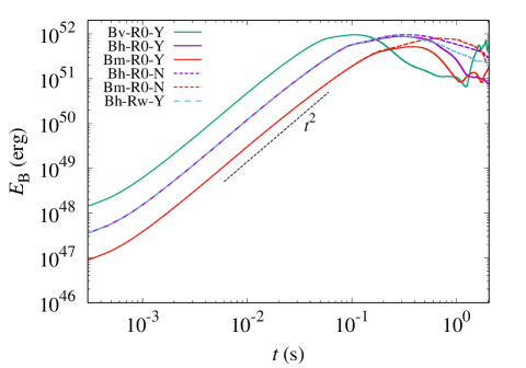
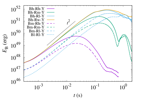
Figure 1: Evolution of the electromagnetic energy for all the ideal MHD models, Bv-R0-Y, Bh-R0-Y, Bh-R0-N, Bm-R0-Y, Bm-R0-N, and for a resistive model with a high conductivity, Bh-Rw-Y (left panel) and for all the resistive models employed in this paper (right panel).

In the present context, the typical MHD process in the remnant neutron star of neutron-star mergers in the presence of an initial seed poloidal magnetic field is governed by the magnetic winding effect, for which the growth timescale of the toroidal magnetic-field energy is written approximately by Eq. (57). When the electromagnetic energy exceeds a few % of the rotational kinetic energy of the remnant neutron star (for this case $E_{\rm kin}\approx 1.16\times 10^{53}$ erg), the magnetic braking starts playing an important role. As a consequence, the angular momentum in the neutron star is redistributed and the differentially rotating configuration of the angular velocity is enforced to approach a (approximately) rigidly rotating one. Then, the angular velocity in the central region exceeds $\sim 5000$ rad/s (i.e., the rotational period is $\sim 1.2$ ms). After the toroidal magnetic-field strength is significantly increased by the winding, the mass outflow from the neutron-star surface is enhanced by the increased magnetic pressure (although the mass ejection in the present context is driven primarily by the neutrino irradiation/heating: see Sec. III.2). After the magnetic braking works significantly, the increase of the angular velocity in the central region is decelerated. In addition, the magnetic-field profile in the neutron star is modified significantly by the mass outflow (and resulting magnetic-flux escape) process. The detail on these findings is described in Sec. III.1.1.

In the presence of only low resistivity (i.e., a high value of $\sigma_{\rm c}$), the evolution process of the remnant neutron star is essentially the same as in the ideal MHD case. In the presence of a high resistivity with which the dissipation timescale of the magnetic field is shorter than the winding timescale, not only the winding but also the magnetic-field dissipation plays an important role. For such cases, the magnetic winding does not occur significantly and the magnetic-field effect on the angular velocity profile is minor (see Sec. III.1.2 for details).

III.1.1 Ideal MHD

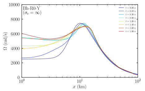
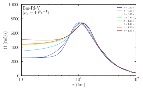
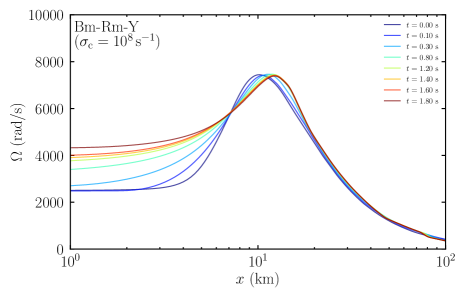
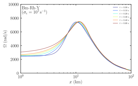
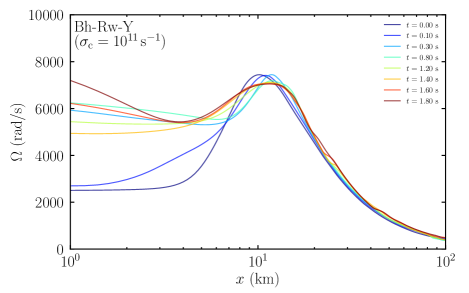
Figure 2: Evolution of the angular velocity profile for models Bh-R0-Y (top left), Bm-R0-Y (top right), Bm-Rl-Y (middle left), Bm-Rm-Y (middle right), Bm-Rh-Y (bottom left), and Bh-Rw-Y (bottom right). We note that due to the neutrino cooling, the remnant neutron star contracts and its central region spins up. For model Bm-Rh-Y, the increase of the angular velocity is predominantly due to this effect.

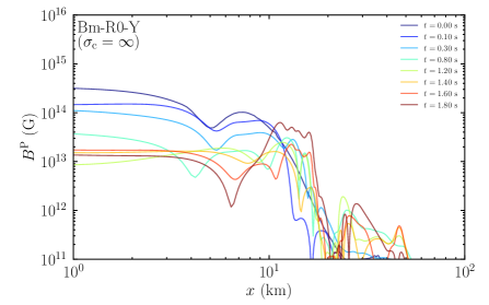
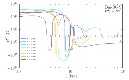
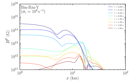
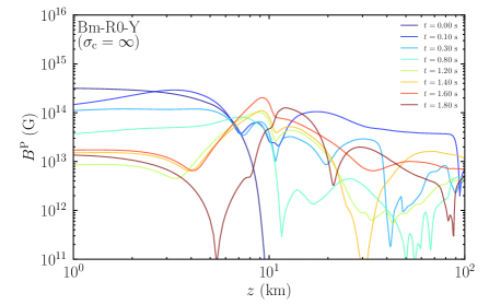
Figure 3: Poloidal (left) and toroidal (right) magnetic-field strength along the $x$-direction with $z=1$ km at selected time slices for models Bm-R0-Y (top panel), Bm-R0-N (2nd top panel), and Bm-Rm-Y (3rd panel). The bottom panel shows the poloidal and toroidal magnetic-field strengths along the $z$-direction with $x=1$ km for model Rm-B0-Y. The field strengths of the poloidal and toroidal components are defined by $B^{P}=\sqrt{{\cal{B}}^{x}{\cal{B}}_{x}+{\cal{B}}^{z}{\cal{B}}_{z}}\gamma^{-1/2}$ and $B^{T}={\rm sign}({\cal{B}}^{y})\sqrt{{\cal{B}}^{y}{\cal{B}}_{y}}\gamma^{-1/2}(\approx{\cal{B}}^{y}\gamma^{-1/3})$, respectively.

Figure 1 shows the electromagnetic energy as a function of time. The left panel plots the results for all the ideal MHD models together with one resistive model of a high conductivity (Bh-Rw-Y) and the right panel plots those for all the resistive MHD models. In the ideal MHD cases, the electromagnetic energy, $E_{\rm B}$, is initially increased by the magnetic winding effect by several orders of magnitude. In this early stage, $E_{\rm B}$ is approximately proportional to $t^{2}$ irrespective of the models (including the resistive MHD models except for the case of $\sigma_{\rm c}=10^{7}\,{\rm s}^{-1}$ for which the resistive dissipation timescale is quite short; the order of 10 ms).

For the ideal MHD case, after $E_{\rm B}$ exceeds $\sim 3\%$ of $E_{\rm kin}$, the increases of $E_{\rm B}$ is decelerated (i.e., the slope of $E_{\rm B}$ becomes shallower than $t^{2}$), indicating that the winding effect is weaken and the magnetic braking becomes important. However, the increase of $E_{\rm B}$ still continues until it reaches $\sim 10\%$ of $E_{\rm kin}$, and then, the growth of the electromagnetic field is saturated. The saturation energy is slightly smaller for the smaller initial field strength. This is primarily due to the fact that more magnetic fluxes are escaped associated with the mass outflow for longer-term evolution, and may be partly due to the numerical dissipation, i.e., in the longer-term evolution the damage by the numerical dissipation is more serious: We note that the simulations are always performed for $\sim 10^{3}$ rotational period of the neutron star.

The saturated energy is slightly higher in the absence of the neutrino irradiation/heating and pair-annihilation effects. Our interpretation for this is that in the absence of these effects, the mass outflow from the neutron star is suppressed (cf. Sec. III.2), resulting escape of the magnetic flux (associated with the mass outflow) is also suppressed, and as a result, the amplification of the electromagnetic field proceeds to a higher level.

As we already mentioned briefly, the mass ejection is driven primarily by the neutrino irradiation/heating (see Sec. III.2 for details). However, with the increase of the electromagnetic energy toward the saturation, the mass ejection from the neutron star is slightly enhanced. This is due to the magnetic pressure primarily resulting from the significantly amplified toroidal magnetic field. By this enhancement of the outflow, a part of the magnetic flux escapes from the neutron star, and as a result, the total electromagnetic energy decreases. However, the decrease rate becomes eventually low ($E_{\rm B}$ eventually shows the oscillatory behavior) and the electromagnetic energy in average appears to relax to $\sim 10^{51}$ erg, i.e., $\sim 1\%$ of the rotational kinetic energy of the neutron star. We note that the rotational kinetic energy does not change significantly by the magnetic braking effects because it is always larger by more than one order of magnitude than the electromagnetic energy, and thus, the magnetic-field effect is minor. Instead, the rotational kinetic energy slightly increases with time because the neutron star contracts due to the emission of neutrinos of total energy of $\sim 10^{53}$ erg, and hence, the neutron star slightly spins up in the absence of the electromagnetic effect, as shown in Ref. [17].

For the nearly ideal MHD case, i.e., for the resistive MHD case with a tiny resistivity (high conductivity, $\sigma_{\rm c}=10^{11}\,{\rm s}^{-1}$; model Bh-Rw-Y), the curve of $E_{\rm B}$ is similar to the corresponding ideal MHD model (Bh-R0-Y) as found in the left panel of Fig. 1. This is natural because for this model, the resistive dissipation timescale is quite long $\sim 100$ s (cf. Eq. (59)). In the late stage with $t\gtrsim 1$ s, the disagreement between the results for models Bh-R0-Y and Bh-Rw-Y is not negligible. Our interpretation for this is that the formulation and the finite-differencing scheme are not completely the same for the ideal and resistive MHD computations; e.g., in the resistive MHD we solve the equations for the electric field but in the ideal MHD we do not. In particular, for regions in which the electromagnetic energy density is much higher than the rest-mass energy density, we have to introduce an artificial treatment to avoid the crush of the computation, and for such regions the prescription becomes different in the two MHD implementations. Hence, in the long-term simulation, the numerical error accumulated by such an artificial treatment could cause this difference (accordingly, for $t\gtrsim 1$ s, the numerical results are not very accurate).

Associated with the magnetic braking by the amplified toroidal magnetic fields, the angular velocity profile of the neutron star is always modified for the ideal MHD case (see top two panels of Fig. 2). As we mentioned in Sec. I, initially, the angular velocity is an increase function of $\varpi$ in the central region of the neutron star. This profile is modified and approaches gradually a rigidly rotating state for the region in which the strong magnetic field is present. Figure 2 illustrates that the angular velocity in the central region is increased by a factor of $\sim 2$ by this effect. Thus, the degree of the differential rotation is reduced by the winding. The timescale for this process is determined by the Alfvén timescale [21, 22]

$$\tau_{\rm a} = {R\over B^{T}/\sqrt{4\pi\rho h}}$$ (61)

$$\approx 0.11\,{\rm s}\left({R\over 10\,{\rm km}}\right)\left({B^{T}\over 10^{15}\,{\rm G}}\right)^{-1}\left({\rho\over 10^{15}\,{\rm g/cm^{3}}}\right)^{1/2},$$

where $R$, $B^{T}$, and $\rho$ denote the typical radius, toroidal magnetic-field strength, and rest-mass density of the neutron star, and we set $h\approx 1$ for simplicity. Unless the magnetic-field profile is significantly modified, after the magnetic braking occurs, the angular velocity should basically show oscillatory behavior with the timescale of $\tau_{\rm a}$, because the angular velocity approximately obeys a hyperbolic equation [21]. However, in the present context, the poloidal magnetic flux is significantly escaped by the neutrino-driven mass outflow and a simple oscillation is not seen. We also note that in the non-axisymmetric case, the turbulence and dynamo effects also would modify the magnetic-field profile significantly [23].

The top and bottom panels of Fig. 3 show the poloidal (left) and toroidal (right) magnetic-field strength along $x$-direction with $z=1$ km (top) and along the $z$-direction with $x=1$ km (bottom) for model Rm-B0-Y. The poloidal and toroidal magnetic-field strengths are defined, respectively, by $\sqrt{{\cal{B}}^{x}{\cal{B}}_{x}+{\cal{B}}^{z}{\cal{B}}_{z}}\gamma^{-1/2}$ and ${\rm sign}({\cal{B}}^{y})\sqrt{{\cal{B}}^{y}{\cal{B}}_{y}}\gamma^{-1/2}(\approx{\cal{B}}^{y}\gamma^{-1/3})$. It is found that the toroidal-field strength (absolute value) is increased far beyond $10^{15}$ G inside the neutron star quite uniformly. By contrast, the maximum value of the poloidal field strength does not increase but rather decreases in the late phase. This decrease is due to the fact that associated with the matter outflow, the magnetic flux is ejected from the neutron star. By this process, instead, a strong poloidal field is produced in the polar direction outside the neutron star (see the bottom panels of Fig. 3): The typical poloidal-field strength at the neutron-star pole is $\sim 10^{14}$ G and $\sim 10^{13}$ G at $z\sim 100$ km.

Associated with the mass outflow from the neutron-star surface, magnetic-fluxes escape toward a large $\varpi$ and large $z$ direction. Because the angular velocity of the escaped matter decreases with the motion toward $\varpi$-direction, the generation of a negative toroidal magnetic field is proceeded along the field lines of the escaped matter. This effect subsequently makes the toroidal magnetic field in the neutron star negative. For model Bm-R0-Y, the mass outflow from the neutron-star surface is appreciably caused by the neutrino-driven wind. As a result, the region with the negative toroidal field expands gradually with time (see the top-right panel of Fig. 3). By contrast, for model Bm-R0-N, the neutrino-driven wind is absent and the mass outflow from the neutron-star surface is weak. Consequently, the region with the negative toroidal field appears only in the vicinity of the neutron star surface (see the second-top-right panel of Fig. 3).

As indicated in Fig. 3, the toroidal magnetic-field energy dominates over the poloidal magnetic-field one after the significant winding: The poloidal-field energy is $<0.1\%$ of the toroidal field energy. However, this may be an artifact in axisymmetric computations in which no dynamo effect is present [26]. In reality, the poloidal-field strength may become much higher than the present results.

III.1.2 Resistive MHD

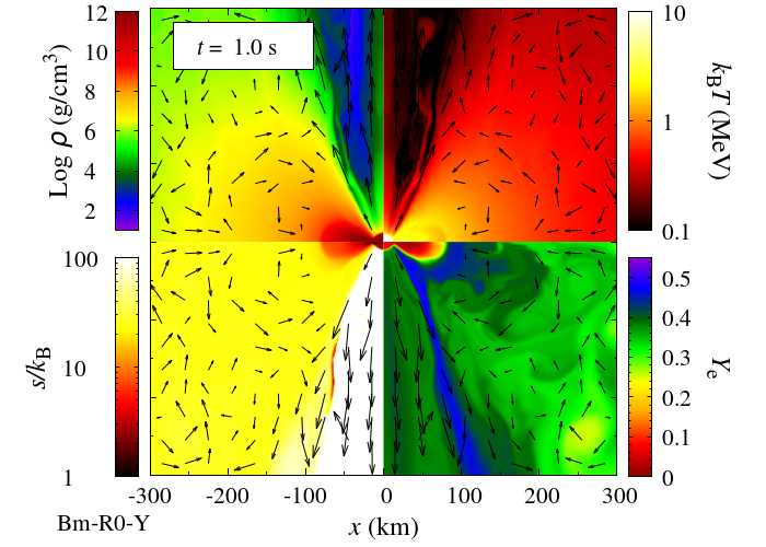
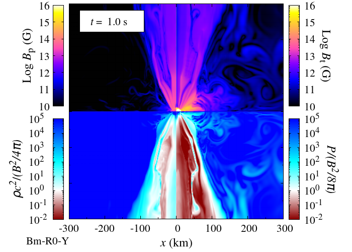
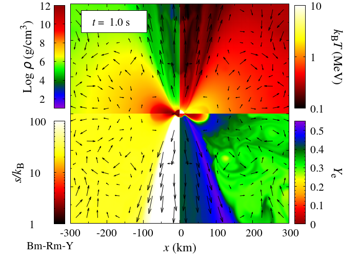
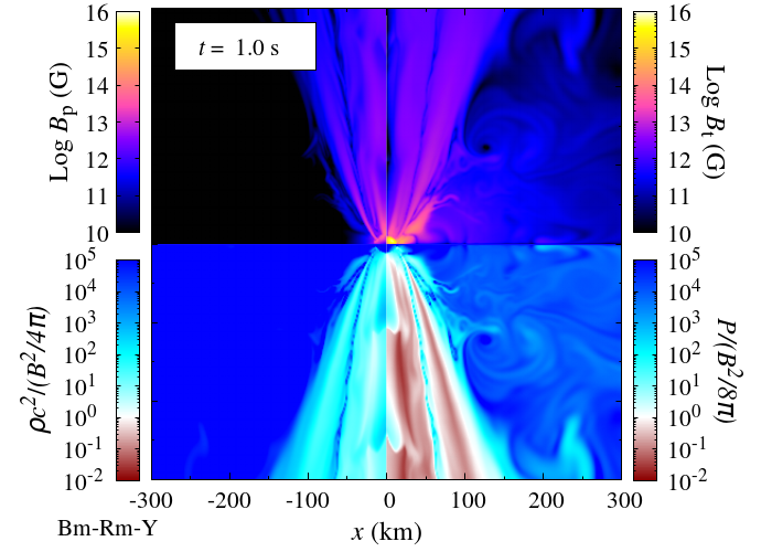
Figure 4: Profiles for the density, temperature, specific entropy, electron fraction (left for these four plots), poloidal and toroidal magnetic-field strength, the ratio of the rest-mass to magnetic energy density, and the ratio of the gas pressure to the magnetic pressure (right for these four plots) after the saturation of the growth of the electromagnetic field for models Bm-R0-Y (top panels) and Bm-Rm-Y (bottom panels).

For the resistive MHD models with low values of the conductivity (i.e., high resistivity), the magnetic-field strength and the maximum value of $E_{\rm B}$ reached by the magnetic winding depend on the values of $\sigma_{\rm c}$, and thus, are different from those for the ideal MHD case (see the right panel of Fig. 1 as well as Figs. 2 and 3). Specifically, the maximum magnetic-field strength depends on the ratio, $\tau_{\rm dis}/\tau_{\rm wind}=:R_{\tau}$: For smaller values of $R_{\tau}$ (i.e., $R_{\tau}\lesssim 1$), the maximum values of the magnetic-field strength and $E_{\rm B}$ are smaller because the resistive dissipation of the electromagnetic energy proceeds faster than the magnetic winding. Thus, for the smaller values of the initial electromagnetic energy, these maximum values are smaller for a given value of $\sigma_{\rm c}$. This is found clearly from the results for $\sigma_{\rm c}=10^{7}$ and $10^{8}\,{\rm s}^{-1}$ (compare the results of models Bh-Rm-Y and Bh-Rh-Y with Bm-Rm-Y and Bm-Rh-Y, respectively). By contrast, for $R_{\tau}\gtrsim 1$, the resistive effect is not very remarkable: For example, the maximum value of $E_{\rm B}$ always exceeds 1% of the rotational kinetic energy, $E_{\rm kin}$, because the magnetic winding sufficiently proceeds until the saturation of the growth is reached: See the results with $\sigma_{\rm c}\geq 10^{9}\,{\rm s}^{-1}$.

We note that irrespective of the maximum value of $E_{\rm B}$ reached, the toroidal magnetic-field energy dominates over the poloidal magnetic-field one in the end as in the ideal MHD case. Again, this could be an artifact in axisymmetric computations with no dynamo effect in which the poloidal field cannot be amplified [26]. In the non-axisymmetric case, this is unlikely to be the case, and hence, the poloidal field may be also enhanced in the later stage.

For the case that the maximum value of $E_{\rm B}$ is smaller than $\sim 3\%$ of $E_{\rm kin}$, the effect of the magnetic braking is weak, and hence, the differential rotation is modified weakly. As found from the middle-right and bottom-left panels of Fig. 2, the angular velocity near the rotational axis ($x=0$) does not increase appreciably for $\sigma_{\rm c}\leq 10^{8}\,{\rm s}^{-1}$ (see also footnote 1). By contrast, the angular-velocity profile for $\sigma_{\rm c}\geq 10^{9}\,{\rm s}^{-1}$ evolves in a similar manner to that in the ideal MHD case (compare the top-left and bottom-right panels or the top-right and middle-left panels of Fig. 2).

The third row of Fig. 3 shows the evolution of the magnetic-field profile near the equatorial plane for a resistive model (Bm-Rm-Y). Figure 3 illustrates that the magnetic-field strength depends strongly on $\sigma_{\rm c}$: For $\sigma_{\rm c}\leq 10^{8}\,{\rm s}^{-1}$, the magnetic field is dissipated in $0.1$ s and the resulting field strength is by 1–2 orders of magnitude smaller than that in the ideal MHD case (compare the top and third-top panels of Fig. 3). For model Bm-Rm-Y, the toroidal field component varies from the positive to negative values in the neutron star for late times. As we mentioned our interpretation for this by an analysis at the end of Sec. II, this reflects the resistive evolution of the toroidal magnetic field in axial symmetry.

For the case that the resistive dissipation timescale is short, $\lesssim 0.1$ s, the thermal energy is generated in the phase in which the neutrino-driven mass outflow is most efficient. However, for such cases, $R_{\tau}$ is small, $<1$, and hence, the electromagnetic energy caused by the winding is much smaller than the rotational kinetic energy and internal energy of the neutron star. Hence, the generated thermal energy plays only a minor role for the mass outflow and evolution of the neutron star (although this may contribute a bit to enhancing the mass ejection). For $R_{\tau}\gtrsim 1$, the electromagnetic energy reached is $\sim 10\%$ of the rotational kinetic energy. For such cases, however, the dissipation timescale is quite long; in our present setting, it is longer than $\sim 1$ s. Since the timescale for launching the neutrino-driven outflow is shorter than or as short as this timescale, the thermal energy generated by the resistive dissipation is not likely to play a major role for the evolution of the remnant neutron stars and mass ejection.

III.1.3 Outcome after the winding

Figure 4 displays the profiles for the density, temperature, specific entropy, electron fraction (left for these four plots), poloidal and toroidal magnetic-field strength, the ratio of the rest-mass to magnetic energy density, and the ratio of the gas pressure to the magnetic pressure (right for these four plots) after the saturation of the electromagnetic energy is reached for models Bm-R0-Y (ideal MHD model: top panels) and Bm-Rm-Y (moderately high resistivity model: bottom panels). These plots show that the system is composed of a massive neutron star surrounded by a disk and an outflow driven from the polar region of the neutron star toward the $z$-direction irrespective of the presence or absence of the resistivity.

However, by comparing the profiles for the two models, two quantitative differences are found. First, the magnetic-field strength for Bm-R0-Y is stronger than for Bm-Rm-Y as we already mentioned in Sec. III.1.2 (see Fig. 3). This is clearly reflected outside the neutron star in Fig. 4. Second, the property of the outflow driven from the polar surface of the neutron star depends on the strength of an MHD effect: In the presence of the strong MHD pressure (i.e., the ideal MHD case), the matter density in the polar region is smaller, and also, the velocity of the outflow is higher. This modifies the electron fraction of the matter in the polar region and ejecta: The electron fraction is lower for model Bm-R0-Y for which the outflow velocity is higher and the effect of the neutrino irradiation to the ejecta is weaker (see also Sec. III.2).

III.1.4 Remark: Comparison with previous work

In the present work, we find that the massive neutron star does not contract significantly and its structure is not modified essentially, after the magnetic winding and braking processes. This conclusion is in contrast to previous work [39, 40, 41], which showed that differentially rotating neutron stars significantly contract, and if they are hypermassive, they collapse to a black hole, after the magnetic winding effect and associated angular momentum transport by the magnetic braking take place. The major reason for the absence of the significant contraction is that in the present work, a realistic angular velocity profile is determined by the merger simulation (i.e., $d\Omega/d\varpi>0$ in the central region of the neutron star) while in Refs. [39, 40, 41], they assumed that the angular velocity decreases steeply with the cylindrical radius. For $d\Omega/d\varpi>0$, the centrifugal force in the central region of the neutron star increases after the magnetic winding and subsequent magnetic braking proceed, whereas for $d\Omega/d\varpi<0$ (in the previous work), the centrifugal force in the central region decreases by the magnetic-field effects, and hence, the eventual collapse of the hypermassive neutron stars to a black hole can occur. Moreover, the outward angular momentum transport proceeds efficiently for $d\Omega/d\varpi<0$, while for $d\Omega/d\varpi>0$ (the present case) an inward angular momentum transport occurs. Our present work indicates that the choice of the angular velocity profile is an important factor for exploring a realistic evolution process of the hypermassive neutron stars in numerical simulations.

III.2 Ejecta

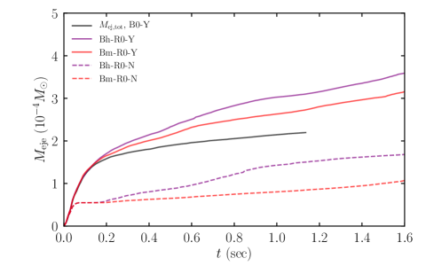
Figure 5: Ejecta mass as a function of time for the ideal MHD cases. Model B0-Y refers to the result in the absence of the magnetic-field effect but with the neutrino effects.

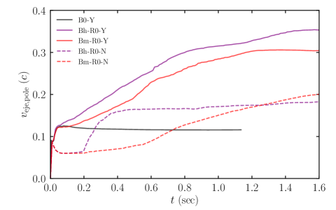
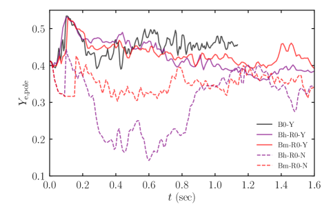
Figure 6: Average velocity (left panel) and electron fraction (right panel) of the ejecta as functions of time for the ideal MHD simulations and for one simulation without the MHD effect (B0-Y).

As we reported in our previous papers [25, 11, 17], the mass ejection proceeds from the remnant of binary neutron star mergers through the neutrino irradiation/heating even in the absence of any other effects like the MHD and viscous effects. The rest mass of this neutrino-irradiation component is not very large as $\lesssim 10^{-3}M_{\odot}$ [25, 17]. In the context of the present paper, the mass ejection may be enhanced by the MHD effect that results primarily from the amplified toroidal magnetic field. In this subsection, we pay attention to this enhancement. Because we finally find that the mass ejection by the magnetic pressure enhanced by the magnetic winding in the neutron star is a minor effect, we here pay attention to this topic focusing only on the ideal MHD results.

The ejecta component is determined using the same criterion as in Refs. [16, 17]; we identify a matter component with $|hu_{t}|>h_{\rm min}$ as the ejecta. Here $h_{\rm min}$ denotes the minimum value of the specific enthalpy in the adopted equation-of-state table, which is $\approx 0.9987c^{2}$. For the matter escaping from a sphere of $r=r_{\rm ext}$, we define the ejection rates of the rest mass and energy (kinetic energy plus internal energy) at a given radius and time by

$$\dot{M}_{\rm eje} := \oint\rho\sqrt{-g}u^{i}dS_{i},$$ (62)

$$\dot{E}_{\rm eje} := \oint\rho\hat{e}\sqrt{-g}u^{i}dS_{i},$$ (63)

where $\hat{e}:=h\alpha u^{t}-P/(\rho\alpha u^{t})$. The surface integral is performed at $r=r_{\rm ext}$ with $dS_{i}=\delta_{ir}r_{\rm ext}^{2}\sin\theta d\theta d\varphi$ for the ejecta component. $r_{\rm ext}$ is chosen to be 1000 km in this work.

$\rho\sqrt{-g}u^{t}(=\rho_{*})$ obeys the continuity equation for the rest mass (see Eq. (1)), and thus, the time integration for it is a conserved quantity. Also in the absence of gravity and magnetic-field effects, $\rho\hat{e}\sqrt{-g}u^{t}$ obeys the energy conservation equation, and far from the central region, the sum of its time integration and its gravitational potential energy are approximately conserved (assuming that the electromagnetic energy is much smaller than the kinetic energy). Thus, the total rest mass and energy (excluding the gravitational potential energy and electromagnetic energy) of the ejecta (which escape away from a sphere of $r=r_{\rm ext}$) are calculated by

$$M_{\rm eje,esc}(t) := \int^{t}\dot{M}_{\rm eje}dt,$$ (64)

$$E_{\rm eje,esc}(t) := \int^{t}\dot{E}_{\rm eje}dt.$$ (65)

Far from the central object, $E_{\rm eje,esc}$ is approximated by

$$E_{\rm eje,esc}\approx M_{\rm eje,esc}c^{2}+U+T_{\rm kin}+{GMM_{\rm eje,esc}\over r_{\rm ext}},$$ (66)

where $U$ and $T_{\rm kin}$ are the values of the internal energy and kinetic energy of the ejecta at $r_{\rm ext}\rightarrow\infty$, respectively. The last term of Eq. (66) approximately denotes the contribution of the gravitational potential energy of the matter at $r=r_{\rm ext}$ with $M$ being the total gravitational mass of the system [16]. Since the ratio of the internal energy to the kinetic energy of the ejecta decreases with its expansion, we may approximate $U/T_{\rm kin}\approx 0$, and hence, $E_{\rm eje,esc}$ by $E_{\rm eje,esc}\approx M_{\rm eje,esc}c^{2}+T_{\rm kin}+GMM_{\rm eje,esc}/r_{\rm ext}$ for the region far from the central object. We then define the average velocity of the ejecta (for the component that escapes from a sphere of $r=r_{\rm ext}$) by

$$v_{\rm eje}:=\sqrt{{2(E_{\rm eje,esc}-M_{\rm eje,esc}c^{2}-GMM_{\rm eje,esc}/r_{\rm ext})\over M_{\rm eje,esc}}}.$$ (67)

In the setting of the present paper, the mass outflow and resulting ejection occur only from the polar region of the neutron star (cf. Fig. 4), because we do not take into account the realistic evolution of the disk surrounding the neutron star, and mass outflow does not occur from it. Thus, in the present work, we perform the surface integral of Eqs. (62) and (63) only for $\theta\leq 15^{\circ}$ where $\theta$ denotes the polar angle. Since the initial condition of our simulations is prepared using the result of a merger simulation for binary neutron stars, the dynamical ejecta component is present from the beginning in the computational domain [17]. However, the dynamical ejecta component is located primarily near the equatorial plane. Thus, with the restriction for the surface integral of $\theta\leq 15^{\circ}$, we can focus approximately on the post-merger mass ejection, which comes primarily from the polar region of the neutron star in the present context.

Figure 5 shows the rest mass of the post-merger ejecta component as a function of time for four ideal MHD simulations. For comparison, we also plot the result in the absence of the magnetic field (but with the neutrino effects: model B0-Y) [17]. Figure 5 shows that the mass ejection is driven primarily by the neutrino irradiation/heating and pair-annihilation heating toward the polar region, because the rest mass of the ejecta in the absence of these neutrino effects is less than half of that in their presence and also less than that in the absence of the magnetic-field effect (model B0-Y). By comparing the results of models Bh-R0-Y and Rm-R0-Y with that of model B0-Y, it is still found that the magnetic pressure enhanced by the magnetic winding increases the ejecta mass. However, as obviously found from Fig. 5, the rest mass of this ejecta component is of the order of $10^{-4}M_{\odot}$ and by two orders of magnitude smaller than that of the viscosity-driven ejecta, which comes from disks (tori) around the neutron star [11, 17]. Therefore, the MHD effect that stems from the winding in the neutron star does not contribute appreciably to increasing the ejecta mass. This is likely to be due to the facts that (i) the MHD effect can strip the material only in a thin polar surface layer of the neutron star for which the total rest mass is tiny and (ii) the gravitational potential near the neutron star is so deep that the mass ejection cannot efficiently occur from its surface.

The present work indicates that the mass ejection by the MHD effect from the neutron star is much less significant than the viscosity-driven mass ejection from disks (tori) surrounding the neutron star. These results suggest that the major source of the mass ejection from the remnant of binary neutron star mergers may be the disk, not the remnant neutron star. However, this speculation should be explored in the future by the simulations in which other important effects such as dynamo effects are taken into account.

A noticeable MHD effect is found in the average velocity and electron fraction of the ejecta (see Fig. 6; cf. Fig. 4 as well). In the absence of the MHD effect (model B0-Y), the average velocity of the ejecta is at most $0.15c$. However, in the presence of the strong MHD effect (models Bh-R0-Y and Bm-R0-Y) the average velocity of the ejecta is enhanced to be $\sim 0.3c$ at $t\sim 1$ s. The comparison of the results for models Bh-R0-Y and Bm-R0-Y with Bh-R0-N and Bm-R0-N (models with no irradiation and pair-annihilation of neutrinos) shows that the neutrino effects also enhance the average velocity by the magnitude similar to that by the MHD effect.

Due to the acceleration by the MHD effect, the influence of the irradiation/heating by neutrinos to the electron fraction of the ejecta becomes weak: In the absence of the MHD effect, the electron fraction of the ejecta becomes always high, $\gtrsim 0.45$, due to the irradiation both by electron neutrinos and anti electron neutrinos, while in the presence of the MHD effect, the electron fraction becomes slightly lower, $\sim 0.4$. For example, for the ideal MHD models Rh-B0-Y and Rm-B0-Y, the electron fraction in the polar region is as high as $\gtrsim 0.4$ before the magnetic field is amplified, but it decreases below $0.4$ after the growth of the magnetic field and associated onset of the accelerated mass outflow. This is due to the fact that the neutron-rich nature of the matter outflowed originally from the neutron-star surface is preserved stronger. Thus, the MHD effect in the neutron star does not contribute much to increasing the ejecta mass, but still has the influence to modify the property of the outflow and ejecta. However, this effect is not as strong as the neutrino irradiation/heating effect (compare models Bh-R0-Y and Bm-R0-Y with Bh-R0-N and Bm-R0-N) as already mentioned.

IV Summary

We performed ideal and resistive MHD simulations for a remnant neutron star of binary neutron star mergers in general relativity with neutrino effects. As a first step, we paid attention to the effect of the magnetic winding for the evolution of the remnant neutron star and resulting mass ejection. The initial matter profile for the simulations was obtained from a merger simulation. A seed poloidal magnetic field, for which the electromagnetic energy is much smaller than the rotational kinetic and internal energy of the system, was initially superimposed inside the remnant neutron star, and we focused only on the evolution of it; we did not pay attention to the MHD evolution of the disk (torus) surrounding the neutron star.

Because of the magnetic winding effect, the toroidal magnetic field is generated and amplified in this setting. Since the toroidal magnetic-field strength increases linearly with time, the electromagnetic-field energy increases as $\propto t^{2}$ in the early growth stage. When the electromagnetic-field energy exceeds $\sim 3\%$ of the rotational kinetic energy, the magnetic braking plays an important role for the redistribution of the angular momentum inside the neutron star. For the ideal MHD case, this always occurs and, as a result of the angular momentum redistribution, the angular velocity, which is initially an increase function of the cylindrical radius, is enforced to approach a rigidly rotating state for the region in which the magnetic braking works well. The maximum electromagnetic energy reached is $\sim 10\%$ of the rotational kinetic energy of the neutron star, i.e., the maximum value of $E_{\rm B}$ is $\sim 10^{52}$ erg. By the angular-momentum redistribution, the rotational kinetic energy of the neutron star is not significantly changed, while at the late stage, the electromagnetic energy relaxes to $\sim 10^{51}$ erg after the magnetic braking is exerted, because the magnetic flux escapes from the neutron star associated with the mass outflow.

For the resistive MHD simulation, the maximum electromagnetic energy reached by the winding effect depends strongly on the magnitude of the conductivity; specifically, the maximum value is determined by the ratio, $R_{\tau}=\tau_{\rm dis}/\tau_{\rm wind}$. For $R_{\tau}\gtrsim 1$, the magnetic winding proceeds until the electromagnetic energy reaches $\sim 10\%$ of the rotational kinetic energy as in the ideal MHD case. On the other hand, for $R_{\tau}<1$, the resistive dissipation plays a role for suppressing the growth of the electromagnetic energy. If the electromagnetic energy does not reach $\sim 3\%$ of the rotational kinetic energy, the magnetic braking effect is weak, and hence, the differentially rotating state of the neutron star is preserved; the increase of the angular velocity near the central region is suppressed.

It is also found that the magnetic field amplified by the winding in the neutron star does not contribute much to enhancing the mass ejection; for the mass ejection from the neutron star, the neutrino effects such as neutrino irradiation/heating and pair-annihilation heating are more important than the MHD effect. Our interpretation for this result is that (i) the MHD effect in the neutron star can strip the material only in the thin polar surface region of the neutron star for which the total rest mass is tiny and (ii) the gravitational potential near the neutron star is so deep that the mass outflow cannot be efficient. The present result suggests that the major source of the mass ejection from the remnant of binary neutron star mergers may not be remnant neutron star but the disk surrounding it. However, this speculation should be examined in more detail by the simulations in which other important effects such as dynamo effects are taken into account.

In the present work, we performed axisymmetric simulations. This implies that we might overlook important MHD effects. One important missing effect is the turbulence induced by Parker [42] and Taylor instabilities [43] (e.g., Ref. [44]). As we showed in this paper, the toroidal magnetic field is inevitably amplified in the presence of a seed poloidal magnetic field. It is well-known that in the presence of the strong toroidal magnetic fields, (non-axisymmetric) Parker and Taylor instabilities can induce a turbulence, which could further induce the magnetic-field amplification through the dynamo effect. It is not clear at all what happens in such a situation. In addition, it is not very clear what the final configuration of the magnetic field profile is after the onset of the turbulence (e.g., Ref. [45]). To explore these questions, we obviously need three-dimensional MHD simulations in the subsequent work. An alternatively phenomenological approach is to incorporate a dynamo term to induce the turbulence state [35, 36]. By this prescription, we do not need three-dimensional simulations: An axisymmetric simulation would be reasonable to obtain some insight on the effect of the turbulence. We plan to perform simulations with a dynamo term in the subsequent work.

Appendix A Test-bed simulations for resistive MHD implementation

We here present the results for a suit of test-bed simulations performed with our resistive MHD implementation. We employed several test-bed problems introduced in Ref. [36] (see also Refs. [46, 47, 48, 49]): the problems of self-similar current sheet, resistive shock tube, and resistive rotor. We also performed test simulations for the propagation of the electromagnetic wave packet in the flat spacetime and for a dynamo closure.

A.1 Self-similar current sheet

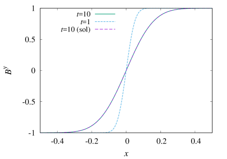
Figure 7: Numerical solution of $B^{y}$ at $t=1$ (dotted curve) and 10 (solid curve) with the analytic solution of Eq. (68) at $t=10$ (dashed curve).

This test-bed problem was first proposed in Ref. [46] and subsequently employed in many references [47, 48, 36, 49]. This is the test to check whether the magnetic field correctly diffuses out with the special-relativistic resistive MHD implementation in the limit that the gas pressure is much higher than the magnetic pressure. In the one dimensional problem in which all the quantities depend only on the $x$ coordinate, an approximate (nearly exact) solution is written, e.g., in the following form:

$$B^{y}(x,t)=C\,{\rm erf}\left({\sqrt{\sigma_{\rm c}}x\over\sqrt{t}}\right),$$ (68)

where erf denotes the error function and $C$ is a constant with $C^{2}/8\pi$ much smaller than the gas pressure. Here we set $C=1$ as the choice of the units for simplicity. Note that our notation for the basic MHD equations is different from the previous papers because of the presence of the factor $4\pi$ in front of $j^{\mu}$ in Eq. (3).

Following Ref. [36], we employ the initial condition at $t=1$ as $\rho=1$, $p=50$, $E^{i}=1$, $u_{i}=0$, $B^{x}=B^{z}=0$, and $B^{y}=B^{y}(x,t=1)$. The $\Gamma$-law equation of state, $p=(\Gamma-1)\rho\varepsilon$ with $\Gamma=4/3$ is employed. $\sigma_{\rm c}$ is set to be $100$ (the resistivity is $1/(4\pi\sigma_{\rm c})$). The computational domain is set up as $x=[-0.6:0.6]$ which is covered by 201 uniform grid points. The simulation is performed until $t=10$. Figure 7 plots $B^{y}$ at $t=1$ and $10$. For $t=10$, we also plot the functional form of $B^{y}$ described in Eq. (68). Figure 7 illustrates that our implementation can reproduce the solution well. In this setting the maximum relative error is $\approx 2.5\times 10^{-4}$.

A.2 Resistive shock tube

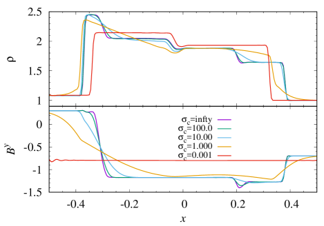
Figure 8: Numerical solutions of $\rho$ (upper panel) and $B^{y}$ (lower panel) for the shock tube test with $\sigma_{\rm c}=10^{10}$, $10^{2}$, 10, 1, and $10^{-3}$. The lower panel plots $B^{y}$ (not $\hat{B}^{y}$).

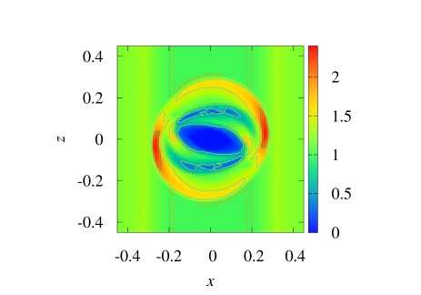
Figure 9: The results of the resistive rotor problem for $\sigma_{\rm c}=10^{10}$ (left) and $1$ (right). The upper and lower panels show $p$ and $E^{z}$, respectively.

This problem was first proposed in Ref. [47]. The initial condition for this problem proposed in Ref. [36] is

$$(\rho,p,v^{x},v^{y},v^{z},\hat{B}^{x},\hat{B}^{y}.\hat{B}^{z})$$

$$=\left\{\begin{array}[]{ll}(1.08,0.95,0.4,0.3,0.2,2.0,0.3,0.3)&{\rm for}~{}x<0,\\ (1.0,1.0,-0.45,-0.2,0.2,2.0,-0.7,0.5)&{\rm for}~{}x\geq 0,\\ \end{array}\right.$$

where $\hat{B}^{i}=B^{i}/\sqrt{4\pi}$ (this renormalization is necessary to align the unit with the previous work) and $v^{i}=u^{i}/u^{t}$. The initial electric field is given by $E^{i}=-\epsilon^{ijk}v_{j}B_{k}$. The $\Gamma$-law equation of state with $\Gamma=5/3$ is employed. $\sigma_{\rm c}$ is chosen to be $10^{-3}$, 1, 10, $10^{2}$, and $10^{10}$. The computation is performed from $t=0$ to $0.55$ covering the computational domain of $x=[-0.5:0.5]$ by 401 uniform grid points. The results are shown for $\rho$ and $B^{y}$ in Fig. 8 as in Ref. [36]. A small unphysical oscillation could be seen for the curves of $\rho$ and $B^{y}$ in the absence of the Kreiss-Oliger dissipation for evolving Maxwell’s equations. However, this dissipation term with a small coefficient of $1/640$ cures the unphysical oscillation. We find that the numerical solutions are quite similar to those found in Ref. [36].

A.3 Resistive rotor

This is a two-dimensional problem with the coordinates $(x,z)$ and the initial condition proposed in Ref. [36] is given in the following manner. Inside a radius of $r=\sqrt{x^{2}+z^{2}}\leq 0.1$, a uniformly rotating medium with $\rho=10$ and the uniform angular velocity of $\Omega=8.5$ is prepared (i.e., $v^{x}=-z\Omega$ and $v^{z}=x\Omega$). Outside the circle of $r=0.1$, on the other hand, we set $\rho=1$ and $\Omega=0$. For the entire region, the pressure and the magnetic field are initially uniform as $p=1$ and $(\hat{B}^{x},\hat{B}^{y},\hat{B}^{z})=(1,0,0)$. The initial electric field is again determined by $E^{i}=-\epsilon^{ijk}v_{j}B_{k}$. The $\Gamma$-law equation of state with $\Gamma=4/3$ is employed, and the system is evolved from $t=0$ to $0.3$.

The computational domain is chosen to be $x=[-0.5:0.5]$ and $z=[-0.5:0.5]$ and is covered by a uniform grid of $401\times 401$ points. This problem is numerically solved for $\sigma_{\rm c}=10^{10}$ (nearly ideal MHD case) and $1$. The results for the profiles of the pressure and $z$-component of the electric field are shown in Fig. 9. By comparing these results with Fig. 3 of Ref. [36], we find a good (qualitative/semi-quantitative) agreement.

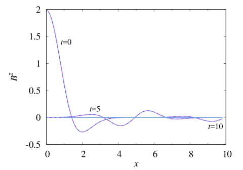
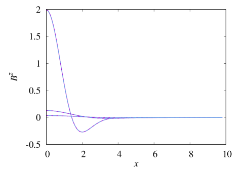
Figure 10: Left: Propagation of electromagnetic waves ($B^{z}$) in the flat spacetime for $\sigma_{\rm c}=0$ at $t=0$, 5, 10, and 15. At $t=15$, the amplitude is much smaller than unity entirely. The solid and dashed curves show the numerical and exact solutions, respectively. Right: Dispersion of electromagnetic waves in the flat spacetime for $4\pi\sigma_{\rm c}=50$ at $t=0$, 50, and 100. The solid and dashed curves show the numerical and exact solutions, respectively (both curves approximately agree). For $x<0$, the solution has the reflection symmetry for both panels (and we do not plot it).

A.4 Evolving electromagnetic fields

To check that our implementation for evolving the electromagnetic fields works well in a practical computational domain, we also performed several test-bed simulations in three spatial dimensions varying the value of $\sigma_{\rm c}$ from $0$ to high values. For $\sigma_{\rm c}=0$ and $\sigma_{\rm c}\rightarrow\infty$ in the flat spacetime of $u_{i}=0$, it is easy to derive analytic solutions for the electromagnetic equations, and thus, we compare the results of the simulations with these analytic solutions.

For $\sigma_{\rm c}=0$, the electromagnetic fields obey wave equations in vacuum, and general solutions for the basic equations are easily derived. For example, an axisymmetric general solution for the dipole radiation is written as

$$B^{r} = {1\over r}{\partial\over\partial r}\left({f(r+t)-f(r-t)\over r}\right)\cos\theta,$$

$$B^{\theta} = -{1\over 2r^{2}}{\partial\over\partial r}\left[r{\partial\over\partial r}\left({f(r+t)-f(r-t)\over r}\right)\right]\sin\theta,~{}~{}$$ (71)

and $B^{\varphi}=0$. For this case, $E^{\varphi}$ is only non-zero component of $E^{i}$ and it is derived straightforwardly from the field equation. Here, $f(u)$ is an arbitrary regular function, and for $f(u)=-ue^{-u^{2}/2}$, the initial condition becomes

$$B^{x} = xze^{-r^{2}/2},$$

$$B^{y} = yze^{-r^{2}/2},$$

$$B^{z} = (2-x^{2}-y^{2})e^{-r^{2}/2},$$ (72)

and $E^{i}=0$. Note here that we choose the width of the wave packet (i.e., unity) as the unit of the length in this problem.

We then evolve this wave packet in the domain of $x=[-10:10]$, $y=[-10:10]$, and $z=[0:10]$ with the grid spacing of $dx=0.1$. The reflection-symmetric boundary condition is imposed on the $z=0$ plane and an outgoing wave boundary condition is imposed on the outer boundaries. The left panel of Fig. 10 plots the numerical profiles of $B^{z}$ along the $x$ axis at $t=0$, 5, 10, and 15 (solid curves) together with the analytic solutions (dashed curves). Note that at $t=15$, the wave packet already propagated away from the computational domain. The relative error of the numerical solution to the analytic one, e.g., at $t=5$, is of order $10^{-3}$ with this setting (except for the outer boundaries). This illustrates that our implementation can well follow the propagation of the electromagnetic waves.

For large values of $\sigma_{\rm c}$, on the other hand, the field equations relax to parabolic ones. For the parabolic equations with the initial condition of Eq. (72), a solution for the dipole magnetic field is written as

$$B^{r} = 2\left(1+{t\over 2\pi\sigma_{\rm c}}\right)^{-5/2}\exp\left(-{r^{2}\over 2+t/\pi\sigma_{\rm c}}\right)\cos\theta,$$

$$B^{\theta} = -{1\over r}\left(1+{t\over 2\pi\sigma_{\rm c}}\right)^{-5/2}\left(2-{r^{2}\over 1+t/2\pi\sigma_{\rm c}}\right)$$

$$\times\exp\left(-{r^{2}\over 2+t/\pi\sigma_{\rm c}}\right)\cos\theta,$$

$$B^{\varphi} = 0.$$ (73)

We again evolve this wave packet in the domain of $x=[-10:10]$, $y=[-10:10]$, and $z=[0:10]$ with $dx=0.1$ and $4\pi\sigma_{\rm c}=50$. The right panel of Fig. 10 plots the profiles of $B^{z}$ along the $x$ axis at $t=0$, 50, and 100 (solid curves) together with the analytic solutions (dashed curves). With the chosen grid resolution, the maximum relative error size is $\approx 4\%$ at $t=100$ (except for the region near the outer boundaries). The largest error is always located near the region at which $B^{z}=0$, and for other regions, the accuracy is much better.

A.5 Steady dynamo

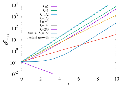
Figure 11: The maximum value of $B^{y}$ for the steady dynamo test for $\sigma_{\rm c}=10$ and $\alpha_{\rm d}=0.2$ with $\lambda_{x}=2$, $1$, $1/2$, $1/3$, $2/7$, $1/4$, $2/9$, $a=0.1$, and $b=0$ (no perturbation in the $z$ direction) and with $\lambda_{x}=1/4$, $\lambda_{z}=1/2$, $a=0.1$, and $b=0.01$. Note that the fastest growing mode has the wavelength of $1/2$ while for the marginally stable mode it is $1/4$. $\lambda$ in the inset of the plot implies $\lambda_{x}$.

Following Ref. [36], we also performed this simple test to check that our implementation works well in the presence of a dynamo term. In this test-bed problem, again, we pay attention only to solving the electromagnetic field setting $u_{i}=0$.

First we assume that $B^{x}=E^{x}=0$, and $B^{y}$, $B^{z}$, $E^{y}$, and $E^{z}$ are functions of $\exp(i\omega t-ikx)$ where $\omega$ and $k$ are the angular frequency and the wave number. Then, the following dispersion relation is derived:

$$\omega^{2}-4\pi i\sigma_{\rm c}\omega-k^{2}\pm 4\pi\sigma_{\rm c}\alpha_{\rm d}k=0.$$ (74)

For this equation, we find that the exponential growth mode is present for the case that $k<4\pi\sigma_{\rm c}\alpha_{\rm d}$, and the resultant expression of $\omega$ is

$$\omega=2\pi i\sigma_{\rm c}\left(1-\sqrt{1-(k/2\pi\sigma_{\rm c})^{2}+k\alpha_{\rm d}/\pi\sigma_{\rm c}}\right),$$ (75)

and for the fastest growing mode with $k=2\pi\sigma_{\rm c}\alpha_{\rm d}$, this becomes

$$\omega=-2\pi i\sigma_{\rm c}\left(\sqrt{1+\alpha_{\rm d}^{2}}-1\right).$$ (76)

Because the basic equation is linear in $E^{i}$ and $B^{i}$, it is straightforward to extend this analysis in the multidimensional case as long as we focus only on the transverse component. That is, for the case that we initially prepare two independent modes proportional to, e.g., $\exp(i\omega t-ik_{x}x)$ and $\exp(i\omega t-ik_{z}z)$ where $k_{x}$ and $k_{z}$ are the wave numbers, the stability of the system is determined simply by analyzing the dispersion relations in the $x$ and $z$ direction independently. Taking into account this fact, we perform two-dimensional simulations setting the region of $x=[-1:1]$ and $z=[-1:1]$ with the periodic boundary conditions in both coordinates.

We then prepare the following initial condition:

$$B^{x} = -b\cos(k_{z}z),$$ (77)

$$B^{y} = a\sin(k_{x}x)+b\sin(k_{z}z),$$ (78)

$$B^{z} = -a\cos(k_{x}x),$$ (79)

and $E^{i}$ is determined by the ideal MHD condition. Here, $a$ and $b$ are constants. In this setting, for the case that $2\lambda_{i}\sigma_{\rm c}\alpha_{\rm d}>1$, the initial seed field should grow exponentially with time, where $\lambda_{i}:=2\pi/k_{i}$ ($i$ is $x$ or $z$) denotes the wave length. Note that our setting of the computational domain can follow the waves only with $\lambda_{i}\leq 2$. Thus, the simulations are performed for $\sigma_{\rm c}=10$ and $\alpha_{\rm d}=0.2$. For this setting, the fastest growing mode has $\lambda_{i}=1/2$ while the marginally stable mode has $\lambda_{i}=1/4$ (i.e., the mode with $\lambda_{i}>1/4$ is unstable).

Figure 11 plots the evolution of the maximum value of $B^{y}$ for $\sigma_{\rm c}=10$ and $\alpha_{\rm d}=0.2$ with $\lambda_{x}=2$, $1$, $1/2$, $1/3$, $2/7$, $1/4$, $2/9$, $a=0.1$, and $b=0$ (no perturbation in the $z$ direction) and with $\lambda_{x}=1/4$, $\lambda_{z}=1/2$, $a=0.1$, and $b=0.01$. The growth rates of the unstable modes are well captured in each simulation. This figure illustrates that our implementation can derive the predicted results irrespective of the prepared initial conditions.

Appendix B Resistive evolution of the massive neutron star with purely toroidal magnetic field

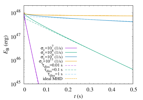
Figure 12: Evolution of the magnetic-field energy for the remnant massive neutron star initially with a purely toroidal magnetic field for $\sigma_{\rm c}=10^{7}$, $10^{8}$, $10^{9}$, and $10^{11}\,{\rm s}^{-1}$ (solid curves). The dashed lines denote $\propto\exp(-t/\tau_{\rm diss})$ with $\tau_{\rm diss}=0.01$, $0.1$, and $1.0$ s for $\sigma_{\rm c}=10^{7}$, $10^{8}$, and $10^{9}$ ${\rm s}^{-1}$, which are consistent with Eq. (59). The result by the ideal MHD implementation is also shown by the dotted curve, which agrees approximately with the curve for $\sigma_{\rm c}=10^{11}\,{\rm s}^{-1}$.

In this section, we present the results for the resistive MHD evolution of the merger remnant neutron star with purely toroidal magnetic fields and demonstrate that our implementation can follow the resistive dissipation of the toroidal magnetic field successfully.

Figure 12 plots the evolution of the electromagnetic energy for the remnant massive neutron star, for which a purely toroidal magnetic field of Eq. (54) is superimposed at $t=0$, in the axisymmetric resistive MHD simulations with $\sigma_{\rm c}=10^{7}$, $10^{8}$, $10^{9}$, and $10^{11}\,{\rm s}^{-1}$ (solid curves). The result of an ideal MHD simulation is shown together (dashed curve). Since the toroidal magnetic field is simply superimposed and thus the initial condition is not exactly in an equilibrium state, the electromagnetic energy initially decreases by 10–20% even in the absence of the resistivity during the early relaxation stage. The subsequent long-term gradual decrease of the electromagnetic energy for the ideal MHD case would be partly due to the numerical dissipation or diffusion. Note again that this evolution process is valid only in the assumption of the axial symmetry. In general cases, non-axisymmetric instability such as Parker and Taylor instability [42, 43] could occur and the evolution process could be significantly modified.

For the resistive MHD case, the magnetic field decreases exponentially with time after the early relaxation stage. The short-dashed slopes denote the relation of $\propto\exp(-t/\tau_{\rm diss})$ where $\tau_{\rm diss}$ is the decay timescale, and are plotted for approximately fitting the curves for the resistive MHD results. It is found that the dissipation timescale of the magnetic field is $\approx 0.01$, $0.1$, and $1.0$ s for $\sigma_{\rm c}=10^{7}$, $10^{8}$, and $10^{9}\,{\rm s}^{-1}$, which are consistent with the timescales estimated by Eq. (59). For $\sigma_{\rm c}=10^{11}\,{\rm s}^{-1}$, the dissipation timescale would be $\sim 10^{2}$ s, and much longer than the simulation time. Therefore, the result for this case agrees approximately with that in the ideal MHD simulation: Our ideal and resistive MHD implementations can derive approximately the identical results.

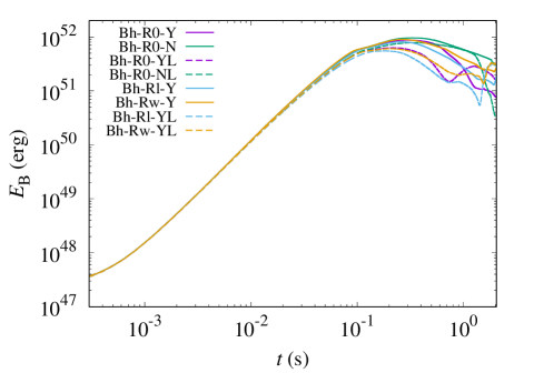
Figure 13: Evolution of the electromagnetic energy for two ideal MHD models Bh-R0-Y, Bh-R0-N and for two resistive MHD models Bh-Rw-Y and Bh-Rl-Y with two different grid resolutions. The solid and dashed curves show the results for $\varDelta x=200$ m and $\varDelta x=250$ m, respectively.

Appendix C Grid resolution dependence

As a convergence test, we performed numerical simulations with two lower grid resolutions for two ideal MHD (Bh-R0-Y and Bh-R0-N) and two resistive MHD (Bh-Rw-Y and Bh-Rl-Y) cases. Figure 13 is the same as Fig. 1 but for the comparison in the evolution of the electromagnetic energy for two different resolutions. The solid and dashed curves show the results for the cases that the neutron star is resolved with the grid spacing of $\varDelta x=200$ m and $\varDelta x=250$ m, respectively.

As found from Fig. 13, the growth of the magnetic-field strength by the winding effect is followed with the lower grid resolution fairly well. However, the amplification of the magnetic-field strength is suppressed for the lower resolution, and thus, the maximum magnetic-field energy becomes smaller. This effect is not appreciable for the case that the effects of the neutrino irradiation/heating and pair-annihilation are switched off. However, in the presence of these neutrino effects, the suppression is quite large: The maximum magnetic-field strength for the lower resolution is by a factor of $\sim 2$ smaller than for the higher one. It appears that the mass ejection associated with these neutrino effects enhance the magnetic-field dissipation or magnetic flux outflow from the neutron star. Thus the poor convergence is likely to be associated with a poor convergence in the neutrino transfer (cf. Ref. [25]).

For the resistive MHD simulations, we also find the tendency similar to that found for the ideal MHD case with neutrino effects. That is, the dissipation or magnetic flux escape from the neutron star is spuriously enhanced for the lower grid resolution. However, overall, the evolution process of the neutron star is not modified qualitatively by the grid resolution.

References

- [1] M. Shibata and K. Hotokezaka, Ann. Rev. Nucl. Part. Sci. 69, 41 (2019).
- [2] B. P. Abbott et al., Phys. Rev. Lett. 119, 161101 (2017).
- [3] LIGO Scientic and VIRGO Collaborations, Astrophys. J. 848, L12 (2017).
- [4] B. D. Metzger and E. Berger, Astrophys. J. 746, 48 (2012).
- [5] K. Hotokezaka and T. Piran, Mon. Not. R. Astron. Soc. 450, 1430 (2015).
- [6] S. A. Balbus and J. F. Hawley, Rev. Mod. Phys. 70, 1 (1998).
- [7] R. Fernández and B. D. Metzger, Mon. Not. Royal Astron. Soc. 435, 502 (2013).
- [8] B. D. Metzger and R. Fernández, Mon. Not. Royal Astron. Soc. 441, 3444 (2014).
- [9] O. Just, A. Bauswein, R. A. Pulpillo, S. Goriely, and H.-Th. Janka Mon. Not. Royal Astron. Soc. 448, 541 (2015).
- [10] D. M. Siegel and B. D. Metzger, Phys. Rev. Lett. 119, 231102 (2017): Astrophys. J. 858, 52 (2018).
- [11] S. Fujibayashi, K. Kiuchi, N. Nishimura, Y. Sekiguchi, and M. Shibata, Astrophys. J. 860, 64 (2018).
- [12] R. Fernández, A. Tchekhovskoy, E. Quataert, F. Foucart, and D. Kasen, Mon. Not. R. Astron. Soc. 482, 3373 (2019).
- [13] A. Janiuk, Astrophys. J. 882, 2 (2019).
- [14] I. M. Christie et al., Mon. Not. R. Astron. Soc. 490, 4811 (2019).
- [15] J. M. Miller et al., Phys. Rev. D 100, 023008 (2019).
- [16] S. Fujibayashi, M. Shibata, S. Wanajo, K. Kiuchi, K. Kyutoku, and Y. Sekiguchi, Phys. Rev. D 101, 083029 (2020).
- [17] S. Fujibayashi, S. Wanajo, K. Kiuchi, K. Kyutoku, Y. Sekiguchi, and M. Shibata, Astrophys. J. 901, 122 (2020).
- [18] R. Fernández, F. Foucart, and J. Lippuner, submitted to Mon. Not. R. Astron. Soc. (arXiv: 2005.14208).
- [19] P. Mösta, D. Radice, R. Haas, E. Schnetter, and S. Bernuzzi, Astrophys. J. 901, L37 (2020).
- [20] M. Shibata, K. Taniguchi, and K. Uryū, Phys. Rev. D 71, 084021 (2005).
- [21] S. L. Shapiro, Astrophys. J. 544, 397 (2000).
- [22] M. Shibata, Y.-T. Liu. S. L. Shapiro, and B. C. Stephens, Phys. Rev. D 74, 104026 (2006).
- [23] L. Sun, M. Ruiz, and S. L. Shapiro, Phys. Rev. D 99, 064057 (2019).
- [24] K. Kiuchi, K. Kyutoku, Y. Sekiguchi, M. Shibata, and T. Wada, Phys. Rev. D 90, 041502 (2014); K. Kiuchi, P. Cerda-Duran, K. Kyutoku, Y. Sekiguchi, and M. Shibata, Phys. Rev. D 92, 124034 (2015); K. Kiuchi et al., Phys. Rev. D 97, 124039 (2018).
- [25] S. Fujibayashi, Y. Sekiguchi, K. Kiuchi, and M. Shibata, Astrophys. J. 846, 114 (2017).
- [26] T. G. Cowling, Mon. Not. R. Astron. Spoc. 94 , 39 (1933).
- [27] M. Shibata, Numerical Relativity (World Scientific, Singapore, 2016).
- [28] M. Shibata and T. Nakamura, Phys. Rev. D 52, 5428(1995): T. W. Baumgarte and S. L. Shapiro, Phys. Rev. D 59, 024007(1998).
- [29] M. Campanelli, C. O. Lousto, P. Marronetti, and Y. Zlochower, Phys. Rev. Lett. 96, 111101 (2006): J. G. Baker, J. Centrella, D.-I. Choi, M. Koppitz, and J. van Meter, Phys. Rev. Lett. 96, 111102 (2006).
- [30] D. Hilditch, S. Bernuzzi, M. Thierfelder, Z. Cao, W. Tichy, and B. Brügmann, Phys. Rev. D 88, 084057 (2013).
- [31] M. Alcubierre, et al., Int. J. Mod. Phys. D 10, 273 (2001).
- [32] M. Shibata, Prog. Theor. Phys. 104 (2000), 325; M. Shibata, Phys. Rev. D 67 (2003), 024033; M. Shibata and Y. Sekiguchi, Prog. Theor. Phys. 127, 535 (2012).
- [33] S. Banik, M. Hempel, and D. Bandyophadyay, Astrophys. J. Suppl. Ser. 214, 22 (2014).
- [34] F. X. Timmes and F. D. Swesty, Astrophys. J. Suppl. 126, 501 (2000).
- [35] A. Brandenburg and K. Subramanian, Phys. Rep. 417, 1 (2005).
- [36] N. Bucciantini and L. Del Zanna, Mon. Not. R. Astron. Soc. 428, 71 (2013).
- [37] M. Shibata and Y. Sekiguchi, Phys. Rev. D 72, 044014 (2005).
- [38] C. R. Evans and J. F. Hawley, Astrophys. J. 332, 659 (1988).
- [39] D. Duez, Y.-T. Liu, S. L. Shapiro, M. Shibata, and B. C. Stephens, Phys. Rev. Lett. 96, 031101 (2006).
- [40] M. Shibata, M. D. Duez, Y.-T. Liu, S. L. Shapiro, and B. C. Stephens, Phys. Rev. Lett. 96, 031102 (2006).
- [41] M. D. Duez, Y.-T. Liu, S. L. Shapiro, M. Shibata, and B. C. Stephens, Phys. Rev. D 73, 104515 (2006).
- [42] E. N. Parker, Astrophys. J., 121, 49 (1955).
- [43] R. J. Tayler, Mon. Not. R. Astron. Soc., 161, 365 (1973).
- [44] K. Kiuchi, S. Yoshida, and M. Shibata, Astron. and Astrophys. 532, A30 (2011).
- [45] V. Duez, J. Braithwaite, and S. Mathis, Astrophys. J., 724, L34 (2010).
- [46] S. S. Komissarov, Mon. Not. R. Astron. Soc. 382, 995 (2007).
- [47] M. Dumbser and O. Zanotti, J. Comput. Phys., 228, 6991 (2009).
- [48] C. Palenzuela, L. Lehner, O. Reula, and L. Rezzolla, Mon. Not. R. Astron. Soc. 394, 1727 (2009).
- [49] Q. Qian, C. Fendt, S. Noble, and M. Bugli, Astrophys. J. 834, 29 (2017).