Hybrid equation of state approach in binary neutron-star merger simulations

Abstract

We investigate the use of hybrid equations of state in binary neutron-star simulations in full general relativity, where thermal effects are included in an approximate way through the adiabatic index $\Gamma_{\text{th}}$. We employ a newly developed finite-temperature equation of state derived in the Brueckner-Hartree-Fock approach and carry out comparisons with the corresponding hybrid versions of the same equation of state, investigating how different choices of $\Gamma_{\text{th}}$ affect the gravitational-wave signal and the hydrodynamical properties of the remnant. We also perform comparisons with the widely used SFHo equation of state, detailing the differences between the two cases. Overall, we determine that when using a hybrid equation of state in binary neutron-star simulations, the value of thermal adiabatic index $\Gamma_{\text{th}}\approx 1.7$ best approximates the dynamical and thermodynamical behavior of matter computed using complete, finite-temperature equations of state.

I Introduction

The numerical simulation of neutron star (NS) mergers requires as a most essential input the equation of state (EOS) of the stellar matter under the relevant conditions of particle composition, partial densities, and temperature.

Comparing and contrasting the results of simulations and of the observed gravitational-wave signal, then allows to constrain theoretical models for the EOS and extract quantitatively the essential features of the EOS. The availability of such data has already permitted this selection process and, in the future, rapid progress is to be expected towards the identification of “the” EOS of dense nuclear matter Abbott et al. (2017, 2018).

Theoretical EOSs have been computed in various approaches, in particular for cold nuclear matter, but much less for hot matter up to the temperatures (about 50 MeV) occurring during the merger. In this article we propose and analyze a finite-temperature EOS derived within the Brueckner-Hartree-Fock (BHF) many-body approach that has already been shown to satisfy all current experimental and observational constraints on nuclear matter Wei et al. (2019a), in particular those imposed by the merger event GW170817 Burgio et al. (2018); Wei et al. (2019b).

We perform here the first binary NS merger simulations with this EOS and investigate, in particular, the effects of different approximations for the treatment of finite temperature in the simulations, following Ref. Bauswein et al. (2010). The motivation is to understand how much the widely used “hybrid-EOS” approach impacts the gravitational-wave properties in binary NS mergers; indeed, since this approach remains the only viable choice when using a zero-temperature EOS, it is important to examine which differences are to be expected with respect to simulations where finite-temperature versions of the same EOS are employed. In this context, the understanding of the best setup to be used in the approximate description is of great importance and can be carried out only by considering the full temperature-dependent EOS. In particular, we have carried out a number of simulations of merging NSs in full general relativity, employing two fully tabulated, temperature dependent EOSs and neutrino-leakage scheme for the treatment of neutrinos. At the same time, we have performed similar simulations employing hybrid EOSs whose cold part is represented by the slice at $T=0$ of the temperature-dependent EOSs and where we have considered a variety of values for the thermal adiabatic index $\Gamma_{\text{th}}$. In this way, and summarising the results of a number of simulations, we conclude that the value of $\Gamma_{\text{th}}\approx 1.7$ best approximates the complete, finite-temperature EOS in binary NS simulations.

The article is organized as follows. We first review in Sec. II the computation of the EOS in the BHF formalism, with different approximation for the finite-temperature part. Our numerical setup and methods are introduced in Sec. III. Results of the simulations are presented in Sec. IV, and conclusions are drawn in Sec. V. Technical details regarding the evaluation of gravitational-wave signal properties are given in the Appendix.

II Equation of state at finite temperature

II.1 The microscopic BHF approach: the V18 EOS

We only provide here a brief overview of the formalism, and refer to the various indicated references for full details, while a more detailed analysis can be found in Lu et al. (2019). We here compute the EOS in the BHF approach for asymmetric nuclear matter at finite temperature Baldo (1999); Nicotra et al. (2006a, b); Li et al. (2010); Burgio et al. (2011); Burgio and Schulze (2010); Bloch and De Dominicis (1958); Lejeune et al. (1986); Baldo and Ferreira (1999). The essential ingredient of this approach is the interaction matrix $K$, which satisfies the following equations

$$K(n_{B},x_{p};E)=V+V\,\real\sum_{1,2}\frac{\ket{12}(1-n_{1})(1-n_{2})\bra{12}}{E-e_{1}-e_{2}+i0}K(n_{B},x_{p};E)\>$$ (1)

and

$$U_{1}(n_{B},x_{p})=\real\sum_{2}n_{2}\expectationvalue{K(n_{B},x_{p};e_{1}+e_{2})}{12}_{a}\,,$$ (2)

where $n(k)$ is a Fermi distribution, $x_{p}\equiv n_{p}/n_{B}$ is the proton fraction, and $n_{p}$ and $n_{B}$ are the proton and the total baryon number densities, respectively. (In the following, we will also use the notation $\rho_{i}\equiv m_{N}n_{i}$ and $\rho\equiv m_{N}n_{B}$ for the rest-mass densities, where $m_{N}=1.67\times 10^{-24}\,{\rm g}$ is the nucleon mass). Here, $E$ is the starting energy and $e(k)\equiv k^{2}\!/2m+U(k)$ is the single-particle energy. The multi-indices $1,2$ denote in general momentum, isospin, and spin. In the present calculations, we adopt the Argonne $V_{18}$ Wiringa et al. (1995) potential as a realistic nucleon-nucleon interaction $V$ supplemented with compatible microscopic three-nucleon forces (TBF), derived by employing the same meson-exchange parameters as the two-body potential Zuo et al. (2002); Li et al. (2008); Li and Schulze (2008); Grangé et al. (1989).

Regarding the extension to finite temperature, we use the so-called frozen-correlations approximation Nicotra et al. (2006a, b); Li et al. (2010); Burgio et al. (2011); Baldo and Ferreira (1999), and approximate the single-particle potentials $U_{n,p}(k)$ by the ones calculated at $T=0$. Within this approximation, the nucleonic free energy density has the following simplified expression,

$$f_{N}=\sum_{i=n,p}\quantity[2\sum_{k}n_{i}(k)\quantity({k^{2}\over 2m_{i}}+{1\over 2}U_{i}(k))-Ts_{i}]\,,$$ (3)

where

$$s_{i}=-2\sum_{k}\quantity(n_{i}(k)\ln n_{i}(k)+\quantity[1-n_{i}(k)]\ln\quantity[1-n_{i}(k)])\,,$$ (4)

is the entropy density for the component $i$ treated as a free Fermi gas with spectrum $e_{i}(k)$. From the total free energy density $f=f_{N}+f_{L}$ including lepton contributions, all relevant observables can be computed in a thermodynamically consistent way, namely one defines the chemical potentials

$$\mu_{i}=\partialderivative{f}{n_{i}}\,,$$ (5)

which allow to calculate the composition of betastable stellar matter, and then the total pressure $p$ and the specific internal energy $\epsilon$

$$p = n_{B}^{2}\partialderivative{(f/n_{B})}{n_{B}}=\sum_{i}\mu_{i}n_{i}-f\,,$$ (6)

$$\epsilon = \frac{f+Ts}{\rho}\,,\quad s=-\partialderivative{f}{T}\,,$$ (7)

so that $e\equiv\rho(1+\epsilon)$ is the total energy density.

In practice, numerical parametrizations for the free energy density of symmetric nuclear matter (SNM) and pure neutron matter (PNM) were given in Ref. Lu et al. (2019), and for asymmetric nuclear matter a parabolic approximation for the $x_{p}$ dependence is used Burgio and Schulze (2010); Zuo et al. (2004); Bombaci and Lombardo (1991); Zuo et al. (1999),

$$f(n_{B},T,x_{p}) \approx f_{\text{SNM}}(n_{B},T)$$

$$+(1-2x_{p})^{2}\quantity[f_{\text{PNM}}(n_{B},T)-f_{\text{SNM}}(n_{B},T)]\,.$$

This specifies the EOS for arbitrary values of baryon density, proton fraction, and temperature, which can then be employed in merger simulations, or simply for computing the mass-radius relation of cold and hot NSs by solving the Tolmann-Oppenheimer-Volkov (TOV) equations for charge-neutral betastable matter including leptons. We also report that the V18 EOS becomes acausal at $n_{B}=0.75\,\text{fm}^{-3}$ ($\rho\approx 1.3\times 10^{15}$ g/cm³; see, e.g., Ref. Taranto et al. (2013)); this density, however, is far from ever being reached in the simulations (see Fig. 4 and related discussion).

Since our EOS, which hereafter we refer to as the V18 EOS, accounts only for homogeneous matter in the core region of the NS, we properly extend the EOS, for every temperature and proton fraction, with an EOS for the crust, which we define as that covering the range in rest-mass densities $\rho\lesssim 10^{14}\,\text{g/cm}^{3}$. In particular, we choose the Shen EOS Shen et al. (2011) for that purpose. Furthermore, an artificial low-density background atmosphere, $\rho\lesssim 10^{3}\,\text{g/cm}^{3}$, evolved as discussed in Radice et al. (2014a), is used in all our simulations.

II.2 The phenomenological SFHo EOS

As an alternative to the temperature-dependent V18 EOS and to extend and strengthen the results of our comparison we have also considered an alternative temperature-dependent EOS, namely, the phenomenological SFHo EOS Hempel and Schaffner-Bielich (2010); Hempel et al. (2012). We recall that phenomenological approaches are commonly used in simulations of core-collapse supernovae and NS mergers, where a wide range of densities, temperatures, and charge fractions, describing both clustered and homogeneous matter, has to be covered. Some of the most commonly used finite-temperature EOSs are the ones by Lattimer & Swesty Lattimer and Swesty (1991) and Shen et al. Shen et al. (1998). In both cases, matter is modelled as a mixture of heavy nuclei treated in the single-nucleus approximation, $\alpha$ particles, and free neutrons and protons immersed in a uniform gas of leptons and photons. In the former case, nuclei are described within the liquid-drop model, and a simplified Skyrme interaction is used for nucleons; in the latter case a relativistic mean field (RMF) model based on the TM1 interaction Sugahara and Toki (1994) is used for nucleons. In both approaches, all light nuclei are ignored, except for alpha particles. This drawback has been overcome in the SFHo EOS model of Hempel & Schaffner-Bielich (HS) Hempel and Schaffner-Bielich (2010) and Hempel et al. Hempel et al. (2012), which goes beyond the single-nucleus approximation, and takes into account a statistical ensemble of nuclei and interacting nucleons. Nuclei are described as classical Maxwell-Boltzmann particles, and nucleons are treated within the RMF model employing different parameterizations.

Figure 1: Left panel: pressure $p$ and energy density $e$ of betastable matter at $T=0$ as a function of the baryon number density. Right panel: thermal pressure and internal energy density, Eqs. (9), (10) at different temperatures. Results with V18 and SFHo EOSs are compared.

Here, we adopt the new SFHo EOS Steiner et al. (2013), which is based on the HS EOS but implemented with a new RMF parameterization fitted to some NS radius determinations. The new RMF parameters are varied to ensure that saturation properties of nuclear matter are correctly reproduced. In particular, the nuclear incompressibility $K=245\,\text{MeV}$ turns out to be compatible with the currently acceptable range of $240\pm 20\,\text{MeV}$ Colò et al. (2004), which agrees with that predicted from the giant monopole resonances. Moreover, the new parameterization ensures that the symmetry energy at saturation density $J=32.8\,\text{MeV}$ is well within the empirical range $28.5-34.9\,\text{MeV}$ Fiorella Burgio and Fantina (2018), and that the NS maximum mass $M_{\text{TOV}}=2.06\,M_{\odot}$ is (marginally) compatible with the currently strongest observational constraint $M>2.14^{+0.10}_{-0.09}\,M_{\odot}$ Cromartie et al. (2020).

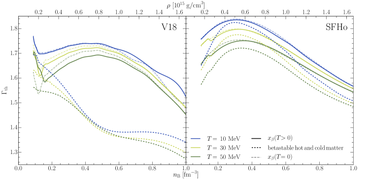
Figure 2: Adiabatic index of betastable matter, Eq. (12), as a function of density at different temperatures. Dashed curves show results obtained from betastable hot and cold matter, while for the solid (dash-dotted) curves the proton fraction is fixed to the one of betastable hot (cold) matter (see discussion in the text).

As an illustration of the properties of these two temperature-dependent EOSs, Fig. 1 shows the pressure $p$ and energy density $e$ of betastable matter as a function of the baryon number density for both the V18 and SFHo EOSs. In particular, in the left panel we display the energy density (solid lines) and pressure (dashed curves) as a function of the baryon density obtained at $T=0$ for the V18 case, and the SFHo EOS. We notice that the V18 EOS is stiffer than SFHo and this will play an important role in the discussion and interpretation of the simulation results. In the right panel, on the other hand, we display the thermal contributions to the betastable EOS defined as

$$p_{\text{th}}(\rho,T) \equiv p(\rho,T)-p(\rho,0)\>,$$ (9)

$$e_{\rm th}(\rho,T) \equiv\rho\quantity[\epsilon(\rho,T)-\epsilon(\rho,0)]\>,$$ (10)

for different temperatures ($T=30,50\,\text{MeV}$) and where $e_{\rm th}$ is the internal energy density. One can notice that in the V18 case the overall thermal effects are smaller than in SFHo, of the order of a few percent at high density, even at the fairly high temperature $T=50\,\text{MeV}$ considered here (see Carbone (2019) for a study on uncertainties of finite-temperature properties of neutron matter). In Ref. Lu et al. (2019) we examined in detail for the V18 case the intricate interplay between the nucleonic and leptonic contributions to the betastable EOS, which are of equal importance.

II.3 Hybrid-EOS approach

An approach often employed in simulations of NS mergers Janka et al. (1993); Bauswein et al. (2010); Baiotti et al. (2008); Hotokezaka et al. (2011); Kiuchi et al. (2014); De Pietri et al. (2016); Endrizzi et al. (2016); Hanauske et al. (2017); Ciolfi et al. (2017); Shibata and Kiuchi (2017); Radice et al. (2018a, b); Alford et al. (2018); Endrizzi et al. (2018); Kiuchi et al. (2019); De Pietri et al. (2020) is the so-called “hybrid-EOS”, in which pressure and the specific internal energy can be expressed as the sum of a “cold” contribution, obeying a zero-temperature EOS, and of a “thermal” contribution obeying the ideal-fluid EOS (see Rezzolla and Zanotti (2013) for details). In this approach, the relation between the thermal pressure and the internal energy density of betastable matter can be expressed as

$$p_{\text{th}}(\rho,T)=e_{\rm th}(\Gamma_{\text{th}}-1)\,.$$ (11)

where $\Gamma_{\text{th}}$ is the thermal adiabatic index appearing in the ideal-fluid approximation. In a temperature-dependent approach, this quantity becomes dependent on density and temperature, i.e., $\Gamma_{\text{th}}\equiv 1+p_{\text{th}}/e_{\rm{th}}$, and this dependence is illustrated in Fig. 2 with dashed curves for the V18 (left panel) and for the SFHo EOS (right panel). Note that there is a clear density dependence, whereas the temperature dependence turns out to be less pronounced. Overall, the thermal adiabatic index remains above $1.5$ at all densities in the SFHo case, but decreases below 1.5 in the V18 case, consistent with the thermal pressures shown in Fig. 1.

In temperature-dependent EOSs to be used in numerical simulations, the adiabatic index is usually not defined for betastable matter (featuring different proton fractions in hot and cold matter), but can be computed at constant proton fraction as

$$\Gamma_{\text{th}}(\rho,T)\equiv 1+\frac{p(\rho,x_{\beta},T)-p(\rho,x_{\beta},0)}{\rho\quantity[\epsilon(\rho,x_{\beta},T)-\epsilon(\rho,x_{\beta},0)]}\,,$$ (12)

where $x_{\beta}$ is the betastable proton fraction at either ($\rho,T>0$) or ($\rho,T=0$). This leads to different numerical values that are also displayed in Fig. 2, where the solid (dash-dotted) curves display results with $x_{\beta}$ taken at $T>0\,(T=0)$ for the V18 (left panel) and the SFHo EOS (right panel), respectively. We note that this procedure yields values $1.5\lesssim\Gamma_{\text{th}}\lesssim 1.7$ for the V18 EOS, and $1.6\lesssim\Gamma_{\text{th}}\lesssim 1.8$ for the SFHo EOS, whereas the average value for the betastable matter is smaller in both cases. We point out, however, that in the merger simulations the matter in the early remnant is usually not in beta equilibrium and therefore all the values shown in Fig. 2 can only give qualitative indications of effective $\Gamma_{\text{th}}$ values. This will be discussed in more detail later.

In fact, three-dimensional hydrodynamical calculations of NS mergers in the conformally flat approximation of general relativity reported in Ref. Bauswein et al. (2010) have questioned the validity of a constant-$\Gamma_{\text{th}}$ approximation in the hybrid-EOS approach (originally chosen as $\Gamma_{\text{th}}\approx 1.5$ Janka et al. (1993)), especially in the postmerger phase, where thermal effects are most relevant. Strong variations were found in both the oscillation frequency of the forming hypermassive NS (HMNS), and the delay time between the merger and black-hole formation, with respect to the simulations with a fully consistent treatment of the temperature. It is one of our goals here to reconsider – by comparing and contrasting fully general-relativistic simulations with temperature-dependent and hybrid EOSs – the issue of the most appropriate constant value of $\Gamma_{\text{th}}$ to be employed when adding a thermal component to the EOS.

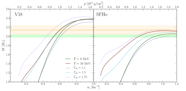
Figure 3: Gravitational mass as a function of the central rest-mass density relations for $T=0$ and $T=50\,\text{MeV}$ with full temperature treatment, and different choices of constant $\Gamma_{\text{th}}=1.1,1.5,1.75$ at $T=50\,\text{MeV}$. Dashed orange and green lines, together with the shaded regions of the same color, refer to the observational constraints of Refs. Cromartie et al. (2020); Antoniadis et al. (2013), respectively.

II.4 Macroscopical properties of the V18 and SFHo EOSs

Given the widespread recent use of hybrid EOSs Kiuchi et al. (2014); Takami et al. (2014, 2015); Rezzolla and Takami (2016); De Pietri et al. (2016); Endrizzi et al. (2016); Hanauske et al. (2017); Ciolfi et al. (2017); Shibata and Kiuchi (2017); Radice et al. (2018a, b); Alford et al. (2018); Endrizzi et al. (2018); Kiuchi et al. (2019); De Pietri et al. (2020) and the scarcity of fully temperature dependent EOSs (that are effectively restricted to a handful Banik et al. (2014); Typel et al. (2010); Steiner et al. (2013); Hempel et al. (2012); Togashi et al. (2016); Most et al. (2020)), the determination of the most realistic value to be used for $\Gamma_{\text{th}}$ is not purely academic. Indeed, even at the lowest-order approximation, $\Gamma_{\text{th}}$ has an impact on the stability of the merger remnant and hence of its lifetime before collapsing to a black hole. This is most easily shown in Fig. 3, which reports sequences of nonrotating equilibrium models as a function of the central rest-mass density (or baryon number density) for the V18 EOS (left panel) and the SFHo EOS (right panel). Different curves refer to different temperatures (i.e., $T=0$ and $T=50\,\text{MeV}$), using the exact temperature dependence and three different choices of constant $\Gamma_{\text{th}}=1.1,1.5,1.75$. In other words, we use Eq. (10) at $T=50\,\text{MeV}$ and the estimate of the thermal adiabatic index to compute the thermal contribution to the pressure, Eq. (11) .

Note the weak dependence of the maximum TOV mass on the temperature, so that for the V18 EOS we have that $M_{\text{TOV}}(T=0)\equiv M_{\text{TOV}}=2.387\,M_{\odot}$ at a central rest-mass density $\rho_{c}=1.58\times 10^{15}\,\text{g/cm}^{3}$ (corresponding to a baryon number density $n_{c}=0.96\,\text{fm}^{-3}$), while $M_{\text{TOV}}(T=50\,\text{MeV})=2.372\,M_{\odot}$ at $\rho_{c}=1.53\times 10^{15}\,\text{g/cm}^{3}$ ($n_{c}=0.93\,\text{fm}^{-3}$). This is mainly due to the competition of three different effects for fixed density and increasing temperature, namely a) the increase of the thermal pressures of neutrons and protons, b) the increase of the isospin symmetry due to beta-stability, which reduces the baryonic pressure, and c) the increase of the lepton thermal pressure. In particular, the V18 EOS is characterized by large values of the symmetry energy which increases with temperature and density, and this is due to the strongly repulsive character of the microscopic three-body forces. This implies a strong increase of the isospin symmetry with temperature and density Lu et al. (2019).

In Fig. 3, left panel, the $\Gamma_{\text{th}}=1.5$ approximation at $T=50\,\text{MeV}$ happens to yield a very similar result as the full calculation, hence we can conclude that for the V18 EOS, the value of the adiabatic thermal index $\Gamma_{\text{th}}=1.5$ represents the best approximation for betastable matter at finite temperature as it is the one that best mimics the effects of a full temperature dependence. The proton fraction $x_{p}$ corresponding to betastability is quite different at $T=0$ and finite $T$ at given baryon density, and therefore the $\Gamma_{\text{th}}$ computed in this way is different from the one calculated at the same $x_{p}$ in both cold and hot matter, using either the $x_{p}$ of cold matter or the one of hot matter in Eq. (12). The latter is the choice made in the numerical simulations and, according to Fig. 2, typical values of $\Gamma_{\text{th}}\sim 1.7$ in this choice correspond to typical values of $\Gamma_{\text{th}}\sim 1.5$ in the betastable procedure, which is the one used in Fig. 3.

On the other hand, $\Gamma_{\text{th}}=1.1$ and 1.75 predict lower and higher $M_{\text{TOV}}$, respectively, according to the lower and higher thermal pressure they provide. One can appreciate the opposite effects of $p_{\text{th}}$ and $e_{\rm th}$ on the maximum mass: when including only $e_{\rm th}$ ($\Gamma_{\text{th}}=1.1$ curves featuring very small $p_{\rm th}$), $M_{\text{TOV}}$ decreases with respect to the cold $M_{\text{TOV}}(T=0)$, whereas including also $p_{\text{th}}$ (FT, $\Gamma_{\text{th}}$=1.5, 1.75 curves) $M_{\text{TOV}}$ increases again. For the V18 FT EOS there is nearly compensation between both effects due to a relatively low thermal pressure, induced by a strong change of the proton fraction in hot vs cold matter, and the related changes of hadronic and leptonic contributions to the pressure that compete with each other, as explained before.

The right panel of Fig. 3 reports the corresponding results for the SFHo case, and in this case we can note a larger temperature dependence of the maximum TOV mass when compared to the V18 case; in turn, this relates to the higher thermal pressure and adiabatic index for the SFHo. This is due to the smaller change of the proton fraction with increasing temperature, which causes a larger thermal pressure, at variance with the V18 EOS case. Consequently, the full calculation at $T=50\,\text{MeV}$ seems to be better reproduced by the $\Gamma_{\text{th}}\simeq 1.7$ approximation here.

The maximum masses are then $M_{\text{TOV}}(T=0)\equiv M_{\text{TOV}}=2.058\,M_{\odot}$, with a central rest mass density $\rho_{c}=1.90\times 10^{15}\,\text{g/cm}^{3}$ ($n_{c}=1.15\,\text{fm}^{-3}$), and $M_{\text{TOV}}(T=50\,\text{MeV})=2.126\,M_{\odot}$, with $\rho_{c}=1.68\times 10^{15}\,\text{g/cm}^{3}$ ($n_{c}=1.02\,\text{fm}^{-3}$). These values, together with other useful information such as the rotation frequencies at the mass-shedding limit, are summarized in Table 1.

Table 1: Properties of the maximum mass configurations of both static and maximally rotating stars with Kepler frequency at temperatures $T=0$ and $50\,\text{MeV}$: gravitational and baryonic masses $M$ and $M_{B}$, and the equatorial radius $R$.

EOS	$f$	$T$	$M$	$M_{B}$	$R$
	[Hz]	[MeV]	[$\,M_{\odot}$]	[$\,M_{\odot}$]	[km]
V18	0	0	2.387	2.913	10.86
	0	50	2.372	2.785	11.40
	1770	0	2.845	3.385	14.17
	1590	50	2.724	3.102	15.00
SFHo	0	0	2.058	2.448	10.30
	0	50	2.126	2.450	11.81
	1741	0	2.472	2.911	13.73
	1376	50	2.413	2.726	15.98

Finally, we note that the merger remnant is expected to be rotating differentially and to support a mass which is upper bounded only by the threshold mass to prompt collapse to a black hole, that can be estimated to be Koeppel et al. (2019)

$$M_{\text{th}}=M_{\text{TOV}}\quantity(3.06-\frac{1.01}{1-1.34\,M_{\text{TOV}}/R_{\text{TOV}}})\>.$$ (13)

For the V18 EOS, the threshold mass Eq. (13) amounts to $M_{\text{th}}=3.04\,M_{\odot}$ with $M_{\text{TOV}}/R_{\text{TOV}}=0.324$, whereas in the SFHo case $M_{\text{th}}=2.86\,M_{\odot}$, being $M_{\text{TOV}}/R_{\text{TOV}}=0.295$ (in geometrized units with $c=1=G=M_{\odot}$).

III Initial data and numerical procedure of merger simulations

The mathematical and numerical setup considered here is similar to the one discussed in great detail in Ref. Papenfort et al. (2018); we review here only the main aspects and differences with respect to this reference, referring the interested reader to the latter for additional information. We consider initial data for irrotational binary neutron stars computed using the multi-domain spectral-method code LORENE LORENE ; Gourgoulhon et al. (2001). All initial data have been modeled considering a zero-temperature, beta-equilibrated cut of the full EOS table (which will be labeled from now on as “cold EOS”), and involve, in our case, equal-masses binaries with a gravitational mass $M=1.35\,M_{\odot}$ at infinite separation (corresponding to a total baryonic mass $M_{\rm b}=2.97\,M_{\odot}$ with the V18 EOS and $M_{\rm b}=2.96\,M_{\odot}$ with the SFHo EOS), and an initial separation between the stellar centers of 45 km.

We then proceed to study two different implementations of our finite-temperature EOS:

(a) The fully-tabulated (FT) case, in which a local temperature is obtained by inverting the $e(\rho,x_{p},T)$ entries in the EOS table, using the values of the internal energy density $e$, rest-mass density $\rho$, and proton fraction $x_{p}$ obtained through the solution of the hydrodynamics equations at a given timestep. This temperature is then used to obtain the total pressure $p(\rho,x_{p},T)$ from the same EOS table.

(b) The “hybrid-EOS” method discussed in Sec. II.3, where finite-temperature effects, caused in particular by shock heating during the postmerger phase, are taken into account by enhancing the zero-temperature EOS with an ideal fluid contribution Janka et al. (1993); Rezzolla and Zanotti (2013). In this method, the local pressure is approximated by

$$p=p_{c}+\rho(\epsilon-\epsilon_{c})(\Gamma_{\text{th}}-1)\,,$$ (14)

using the values $\epsilon_{c}(\rho)$ and $p_{c}(\rho)$ of the cold EOS table for betastable matter and the local propagated values of $\rho$ and $\epsilon$. In this case no local temperature (and no proton fraction) can be extracted during the simulation. The adiabatic index $\Gamma_{\text{th}}$ is a constant both in space and time, constrained mathematically and from first principles to be $1\leq\Gamma_{\text{th}}\leq 2$ Carbone and Schwenk (2019). However, in order to properly compare a simulation of type (b) with the corresponding simulation of type (a), the cold part of the hybrid EOS is chosen to match the $T=0$ slice of the temperature-dependent EOS. In this way, the solutions of type (a) and (b) are identical during the inspiral – when shocks are absent or minute and confined to the stellar surfaces – but start to differ after the merger, when thermal effects develop. Clearly, we consider the simulations of type (a) as the most realistic ones and iterate the values of $\Gamma_{\text{th}}$ in simulations of type (b) to find the closest match in the bulk behavior of the matter.

Overall, for our V18 EOS we consider five different binary merger simulations, namely the reference FT case [i.e., one simulation of type (a)] and four additional simulations in which the value of $\Gamma_{\text{th}}$ is varied [i.e., four simulations of type (b)]. In particular, we consider the limiting case of $\Gamma_{\text{th}}=1.1$, representative of the “cold” case with almost absent thermal effects – the case $\Gamma_{\text{th}}=1.5$, which best approximates the V18 EOS in the betastable regime at $T=50\,\text{MeV}$ according to Figs. 2 and 3 – the case $\Gamma_{\text{th}}=1.7$, which best approximates the FT results in the simulations – and, finally, the case $\Gamma_{\text{th}}=1.75$ with the largest thermal contributions, which also represents a common choice in the literature (see Refs. Bauswein et al. (2010); Takami et al. (2015) for discussions on the use of different $\Gamma_{\text{th}}$). In addition, we also perform three more simulations with the SFHo EOS, one in the FT regime and two using the hybrid-EOS approach with $\Gamma_{\text{th}}=1.5$ and $\Gamma_{\text{th}}=1.75$.

All simulations are performed in full GR using the fourth-order finite-differencing code of McLachlan Brown et al. (2009), which is part of the publicly available Einstein Toolkit Loeffler et al. (2012). The code solves the CCZ4 formulation of the Einstein equations Alic et al. (2012, 2013); Bezares et al. (2017), with a “1+log” slicing condition and a “Gamma driver” shift condition (see, e.g., Refs. Alcubierre et al. (2003); Pollney et al. (2007)). The general-relativistic hydrodynamics equations are solved using the WhiskyTHC code Radice et al. (2014b, a, 2015), which uses either finite-volume or high-order finite-differencing high-resolution shock-capturing methods. We employ, in particular, the local Lax-Friedrichs Riemann solver (LLF) and the high-order MP5 primitive reconstruction Suresh and Huynh (1997); Radice and Rezzolla (2012). For the time integration of the coupled set of hydrodynamic and Einstein equations we use the method of lines with an explicit third-order Runge-Kutta method, with a Courant-Friedrichs-Lewy (CFL) number of $0.15$ to compute the timestep.

Although matter compression and shocks increase the temperature of the remnant to several tens of MeV Radice et al. (2010), neutrino emission acts as cooling mechanism and is implemented in the temperature-dependent simulations as only in the latter the electron fraction is consistently evolved in time. In these cases, we treat the effects on matter due to weak reactions using the gray (energy-averaged) neutrino-leakage scheme described in Refs. Galeazzi et al. (2013); Radice et al. (2016), and evolve free-streaming neutrinos according to the ${\rm M0}$ heating scheme introduced in Refs. Radice et al. (2016, 2018b).

To ensure the non-linear stability of the spacetime evolution, we add a fifth-order Kreiss-Oliger-type artificial dissipation Kreiss and Oliger (1973). We employ an adaptive-mesh-refinement approach, where the grid hierarchy is handled by the Carpet driver Schnetter et al. (2004). Such a hierarchy consists of six refinement levels with a grid resolution varying from $h_{5}=0.16\,M_{\odot}$ (i.e., $\sim 236\,{\rm m}$) for the finest level, corresponding to about 40 points covering the NS radius on the equatorial plane at the beginning of the simulation for both the V18 and SFHo models, to $h_{0}=5.12\,M_{\odot}$ (i.e., $\sim 7.5\,{\rm km}$) for the coarsest level, whose outer boundary is at $1024\,M_{\odot}$ (i.e., $\sim 1515\,{\rm km}$). To reduce computational costs, we adopt a reflection symmetry across the $z=0$ plane. While the V18 simulations presented here follow the remnant evolution for a timescale of at least $20\,{\rm ms}$, the SFHo simulations are stopped a few milliseconds after the collapse to a black hole.

Before concluding this Section, a couple of remarks are useful. First, the hybrid-EOS simulations are carried out using the betastable tables at $T=0$, so that the simulation is “forced” to treat betastable matter, corrected with the already-described finite-temperature effects. The FT simulation, on the other hand, is free to drive away from the betastable condition, and indeed this is what happens starting from the very beginning, as we will discuss in the next Section. Second, the simulations employing the V18 EOS discussed here represent the first application of such recently derived and publicly available temperature-dependent EOS V (18).

     

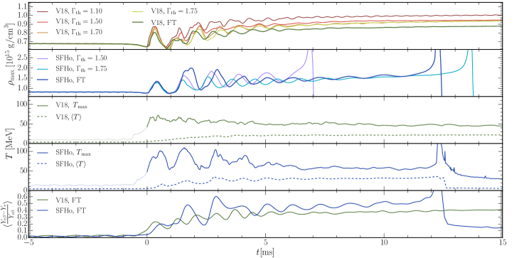
Figure 4: Maximum values of rest-mass density (upper panels) and temperature (third and fourth panels from the top, only for the simulations using the FT EOSs) as a function of time. The evolution of the average temperature $\expectationvalue{T}$, Eq. (15), is also displayed. A lighter color is chosen for the inspiral phase, where such temperatures are meant as representative only and do not reflect an accurate description of the thermodynamics of the matter. The average deviation from beta-stability, Eq. (16), is also represented in the lowest panel for both FT EOSs.

      

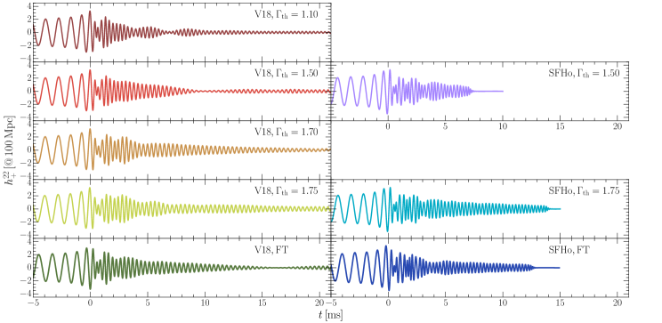
Figure 5: Gravitational waveforms over a time scale of about 20 ms after the merger for the V18 and SFHo EOSs obtained for gravitational masses $2\times 1.35\,M_{\odot}$, comparing different choices of constant $\Gamma_{\text{th}}=1.1,1.5,1.7,1.75$ and the FT EOSs.

IV Numerical results

In the following we present the results of our binary NS mergers simulations. Technical details regarding the extraction of the gravitational-wave signal are given in the Appendix.

IV.1 Bulk dynamics

Following the considerations made in Sec. II for the V18 EOS and the chosen total binary mass $2.7\,M_{\odot}$, the merger simulations do not feature an immediate collapse to a black hole, but produce a metastable HMNS up to the largest time $t\approx 20\,{\rm ms}$ that we reached in the simulations. At that time, the remnant is still stabilized by differential rotation and finite temperature contributions to the pressure. This feature seems to be compatible with the multimessenger analysis of the GW170817 event Gill et al. (2019). On the other hand, the simulations performed with the SFHo EOS lead to a rather rapid collapse into a black hole, which seems to be in contrast with the expected amount of mass ejected in the GW170817 event.

Figure 4 shows in the two top panels the evolution of the maximum rest-mass density, $\rho_{\text{max}}$, for the different cases we have studied, while the third and fourth panel report the evolution of both the maximum and the density-weighted average temperature

$$\expectationvalue{T}\equiv\frac{\int dV\rho\,T}{\int dV\rho}\>,$$ (15)

where the average is performed on the $z=0$ plane, after applying a low-density threshold of $10^{13}\,\text{g/cm}^{3}$ to avoid contamination from the very light but very hot matter ejected; only for the SFHo case, we change this threshold to $10^{10}\,\text{g/cm}^{3}$ in order to also calculate the averaged quantities even after the collapse. A lighter color is chosen for the inspiral phase, where such temperatures are meant as representative only and do not reflect an accurate description of the thermodynamics of the matter. A similar behavior (and even larger inspiral temperatures) has been found also for other temperature-dependent EOSs, e.g., Refs. Most et al. (2019a, b); Perego et al. (2019). In the lowest panel we also show for both FT EOSs the density-weighted average relative deviation from beta stability

$$\expectationvalue{\frac{\Delta Y_{e\beta}}{Y_{e}}}\equiv\frac{\int dV\rho\ \frac{|Y_{e\beta}-Y_{e}|}{Y_{e\beta}}}{\int dV\rho}\>,$$ (16)

where $Y_{e\beta}(\rho,T)$ represents the electron fraction calculated pointwise on the $z=0$ plane assuming beta equilibrium at the density $\rho$ and temperature $T$ of each point. For the V18 EOS it stabilizes at a fairly large reduction of about 40%, which will be discussed later in more detail. We set our time coordinate such that $t=t_{\rm merg}=0$, where $t_{\rm merg}$ is the time of the merger and corresponds to the maximum of the gravitational-wave amplitude, for all the cases we study.

When considering V18-EOS simulations, we find that, unsurprisingly, the $\Gamma_{\text{th}}=1.1$ simulation produces the remnant with the highest maximum rest-mass density ($\rho_{\rm max}\approx 10^{15}\,\text{g/cm}^{3}$), which decreases to about $0.94\times 10^{15}\,\text{g/cm}^{3}$ with increasing $\Gamma_{\text{th}}$. Indeed, this is simply the consequence of the fact that increasing the thermal support against gravity leads to a less dense remnant. Interestingly, the temperature-dependent EOS leads to a remnant with an even smaller maximum rest-mass density ($\rho_{\rm max}\approx 0.88\times 10^{15}\,\text{g/cm}^{3}$) than the hybrid-EOS cases. This feature points to a systematic difference between the two types of simulations: while the hybrid method is by construction based on an EOS of cold betastable matter with thermal corrections, the full simulation produces matter strongly out of beta equilibrium, see the lowest panel of Fig. 4, as will be analyzed later.

On the other hand, the simulations carried out with the SFHo EOS show that the remnant collapses into a black hole after a time which strongly depends on the chosen thermodynamical treatment. In particular, the collapse takes place at $t\approx 13\,{\rm ms}$ for the FT EOS and at $t\approx 7\,{\rm ms}$ or $t\approx 14\,{\rm ms}$ for the cases in which $\Gamma_{\text{th}}=1.50$ or $\Gamma_{\text{th}}=1.75$, respectively. Furthermore, before collapse, the fluctuations of the rest-mass density and temperature are more violent than for the V18 EOS during this metastable phase. While we focus here on the dependence of the collapse time on the temperature treatment, it has also been found to depend sizeably on the numerical resolution (see, e.g. Refs. Kiuchi et al. (2014); De Pietri et al. (2020)), which we have not been able to study here due to lack of numerical resources.

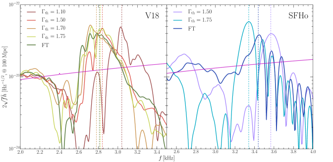
Figure 6: PSDs of the simulations with the V18 and SFHo EOSs, at a distance of 100 Mpc. Vertical dashed lines of different colors indicate the frequency $f_{2}$. The sensitivity curve (magenta color) of Advanced LIGO is displayed for reference.

As mentioned previously, in addition to the maximum temperature for the FT simulations, whose values during the postmerger phase peak at around $70\,\text{MeV}$ and $110\,\text{MeV}$ for the V18 and SFHo EOS respectively, we also report the density-weighted average temperature. Note that for both EOSs, even during the inspiral, the average temperature is much smaller than the maximum values, which, especially during the inspiral, are reached only in small zones of the computational domain, as will be illustrated in Fig. 8.

We also confirm that, while during the inspiral phase there is no great deviation from beta-stability, with average values mostly below 5%, the post-merger remnant manifests important differences with respect to the latter, with average deviations of about 40% and 50% for V18 and SFHo respectively.

IV.2 Gravitational-wave emission

In Fig. 5 we show the plus polarization of the $\ell=m=2$ component of the gravitational-wave strains, which we label as $h^{22}_{+}$, for all the considered simulations we have carried out using the V18 and SFHo EOSs. As expected, no significant differences are found in the inspiral part of the signal, the only notable feature being that the time of merger, which we consider as the time corresponding to the maximum of the strain amplitude, varies slightly when varying $\Gamma_{\text{th}}$ in the hybrid EOS approach (the maximum variations are about $0.05\,{\rm ms}$ with respect to the average times calculated for both EOSs in the hybrid EOS approach). The time of merger measured in the FT runs for both the V18 and the SFHo EOS differs instead of $\approx 0.6\,{\rm ms}$ with respect to the average time calculated in the hybrid-EOS approach; we believe the small difference arises from the fact that while in the hybrid EOS approach finite temperature effects during the inspiral are minimized, the FT approach leads, especially in the final parts of the inspiral, to a temperature increase which, together with the slight deviation of beta-stability, could be responsible for this feature. On the other hand, as clearly shown in Fig. 5, we find that all the cases considered here exhibit very different postmerger profiles.

Figure 6 shows the power spectral density (PSD) plots of all simulations, determined as detailed in the Appendix. In particular, we choose to study the dominant $\ell=m=2$ mode, and consider the position of the $f_{2}$ peak (following the same nomenclature as in Ref. Rezzolla and Takami (2016)) as a tracker of the different behaviors. Since especially for the V18-EOS case with higher $\Gamma_{\text{th}}$ it is difficult to distinguish the dominant $f_{2}$ peaks, a fitting procedure represents the only way for an accurate determination of the $f_{2}$ positions (see the Appendix for a discussion on the determination of the values of the peaks). We report in Table 2 these values, together with their indetermination, the $f_{\text{max}}$ values for each simulation, and the emitted gravitational-wave energy $E_{\text{GW}}$ for the $\ell=m=2$ mode, measured as outlined in the Appendix. In general, $f_{2}$ decreases and $E_{\text{GW}}$ increases with increasing $\Gamma_{\text{th}}$, while the values of $f_{\text{max}}$ depend only very weakly on $\Gamma_{\text{th}}$ and do not show any specific dependence. As a result, and accounting for the fact that the determination of the $f_{2}$ peak frequency inevitably comes with a considerable uncertainty related to the different distributions of power in the various PSDs, the only robust conclusion that can be drawn from the data in Table 2 is that values of the thermal adiabatic index such that $\Gamma_{\text{th}}<1.5$ are not in agreement with the results of the FT simulations. In the following sections we will seek other and more robust indicators of the optimal value for $\Gamma_{\text{th}}$.

Table 2: GW properties of NSs for the considered EOSs: instantaneous frequency at amplitude maximum $f_{\rm{max}}$, frequency of the $f_{2}$ peak, and the total emitted energy $E_{\rm{GW}}$.

Simulation	$f_{\text{max}}\;[\text{kHz}]$	$f_{\text{2}}\;[\text{kHz}]$	$E_{\text{GW}}\;[\text{$10^{52}$ erg}]$
V18 - FT	$1.77$	2.81$\pm$0.02	$5.28$
V18 - $\Gamma_{\text{th}}=1.75$	$1.79$	2.82$\pm$0.08	$5.84$
V18 - $\Gamma_{\text{th}}=1.7$	$1.77$	2.78$\pm$0.07	$5.68$
V18 - $\Gamma_{\text{th}}=1.5$	$1.79$	2.84$\pm$0.01	$4.97$
V18 - $\Gamma_{\text{th}}=1.1$	$1.81$	3.04$\pm$0.01	$4.46$
SFHo - FT	$1.95$	3.44$\pm$0.01	$6.89$
SFHo - $\Gamma_{\text{th}}=1.75$	$1.92$	3.34$\pm$0.01	$7.80$
SFHo - $\Gamma_{\text{th}}=1.5$	$1.93$	3.57$\pm$0.01	$6.38$

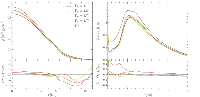
Figure 7: Average rest-mass density and angular velocity for the different V18-based EOSs as a function of the radial coordinate $r$ ($z=0$) at $t=14\,{\rm ms}$.

We further note that the values of the $f_{2}$ frequencies reported in Table 2 agree reasonably well with both the universal relation between $f_{2}$ and the tidal polarizability parameter $k_{2}^{T}$ Rezzolla and Takami (2016) and the radius of a 1.6$\,M_{\odot}$ NS, $R_{1.6}$ Bauswein et al. (2012), which we report for completeness:

$$f_{2}\approx 5.832-1.118\,\left(k_{2}^{T}\right)^{1/5}\approx 2.95\ [\text{kHz}]\,,$$ (17)

$$f_{2}\approx 8.713-0.4667\,R_{1.6}\approx 2.86\ [\text{kHz}]\,,$$ (18)

where $k_{2}^{T}=113.08$, $R_{1.6}=12.54\,{\rm km}$ for the V18 EOS, while $k_{2}^{T}=78.75$, $R_{1.6}=11.77\,{\rm km}$ for the SFHo EOS.

We also find that the simulation employing the V18 EOS with $\Gamma_{\text{th}}=1.1$ yields the highest frequency of the $f_{2}$ peak ($\sim 230\,{\rm Hz}$ above the FT value). Such a finding is in agreement with the behavior of the rest-mass density found in Fig. 4. In particular, since the frequency of the mode scales with the square root of the average density (see, e.g., Ref. Kokkotas and Schmidt (1999)), the behavior of the $f_{2}$ peak confirms spectroscopically that in this case the remnant not only has the largest central density, but it also has the largest average rest-mass density and is therefore subject to the fastest oscillations among all the cases considered.

    

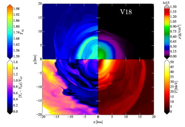
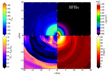
Figure 8: Distributions of $\Gamma_{\text{th}}$, Eq. (12), (upper left side of the figures), rest-mass density (upper right), temperature (lower right), and deviation from beta stability (lower left), in the $z=0$ plane at $t\approx 9\,{\rm ms}$ after the merger.

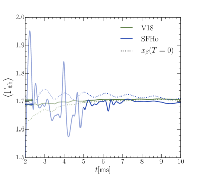
Figure 9: The average $\Gamma_{\text{th}}$, Eq. (19), as a function of time for the FT V18 and SFHo simulations. Time averages related to the total time interval considered here are represented as arrows in the plot. Dotdashed curves represent the average values of $\Gamma_{\text{th}}$ calculated using Eq. (12) with $x_{p}=x_{\beta}(\rho,T=0)$, as described in the text.

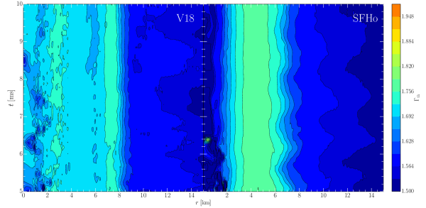
Figure 10: Iso-contours of $\Gamma_{\text{th}}$ as a function of cylindrical radius $r$ and time $t$ for the V18 and SFHo FT simulations.

IV.3 Differential rotation and effective thermal adiabatic index

In the following we analyze in more detail properties of the remnant that is formed after merger. Figure 7, in particular, shows the one-dimensional profiles of the averaged rest-mass density (left panel) and of the angular velocity (right panel) for all the cases we have considered at a time $t\approx 14\,{\rm ms}$ after the merger. The profiles are obtained from the values of the corresponding quantity on the equatorial plane ($z=0$) and after averaging in the azimuthal direction and over a time window of $1\,{\rm ms}$ so as to obtain functions that depend only on the cylindrical radius, $r$, from the center of the grid.

In the bottom part of each panel we also report the fractional differences of the hybrid-EOS profiles with respect to the fiducial FT ones. Overall, we find that in the core of the remnant (i.e., $r\lesssim 6\,{\rm km}$), differences in density remain below $10\%$ for the cases $\Gamma_{\text{th}}=1.5,1.7,1.75$, while they increase below $\rho\approx 2\times 10^{14}\,\text{g/cm}^{3}$. Interestingly, the case $\Gamma_{\text{th}}=1.1$ always shows the largest differences and the case $\Gamma_{\text{th}}=1.7$ the smallest fractional differences in the core area, which is dynamically the most important one.

In order to determine which values of $\Gamma_{\text{th}}$ best approximate the FT behavior, we compute such values pointwise according to Eq. (12), using the local values of $\rho$, $x_{p}$, and $T$ obtained in the FT simulations and the FT tables to compute $p$ and $\epsilon$. Note, however, that while $\Gamma_{\text{th}}$ is used in simulations where the betastability is enforced throughout the evolution, this way of computing $\Gamma_{\text{th}}$ ignores the betastability condition of cold matter, since $x_{p}$ – which is evaluated pointwise in the FT simulations – is not the proton fraction of cold betastable matter. The method is most close to the fixed-$x_{p}$ prescription used in Fig. 1 with $x_{\beta}(T>0)$, but the FT $x_{p}$ is not the one of hot betastable matter either. As a result, it can only give an approximate indication of the “best” value to be used in hybrid-EOS calculations (see also the previous discussion in Sec. II.4).

Figure 8 shows in the top left quadrants the values of the “local” $\Gamma_{\text{th}}$ on the $z=0$ plane at time $t=9\,{\rm ms}$ after the merger. Other quantities reported are: the distributions of the rest-mass density $\rho$ (top right quadrants), the temperature $T$ (bottom right quadrants), and the deviation of the electron fraction from its betastable value, $(Y_{e\beta}-Y_{e})/Y_{e\beta}$ (bottom left quadrants). Note that while in the hybrid-EOS simulations $\Gamma_{\text{th}}$ is, by construction, constant over the computational domain, in the FT case the computed value with the V18 EOS (right panel) is generally $\Gamma_{\text{th}}\lesssim 1.6$ for $\rho\lesssim 5\times 10^{13}\,\text{g/cm}^{3}$, and very close to $\Gamma_{\text{th}}\simeq 1.7$ for higher densities and hence in the core of the HMNS.

On the other hand, the SFHo-simulation (right panel) exhibits a slightly different behavior, with $\Gamma_{\text{th}}\gtrsim 1.7$ in the density region $10^{14}\lesssim\rho/\,\text{g/cm}^{3}\lesssim 10^{15}$ and with the highest-density region being instead dominated by values $\Gamma_{\text{th}}\lesssim 1.65$. This behavior confirms qualitatively the conclusions drawn from Fig. 6, namely, that a value of the thermal adiabatic index $\Gamma_{\text{th}}\approx 1.7$ provides a good match to the post-merger spectroscopic properties observed in the two FT EOSs.

The temperature distributions reported in Fig. 8 show the typical appearance of two hot spots of more than $50\,\text{MeV}$ Kastaun and Galeazzi (2015); Hanauske et al. (2017), whose temperature evolution was shown in Fig. 4 and whose appearance can be associated with the conservation of the Bernoulli constant (see Hanauske et al. (2017) for a detailed discussion). The two hot spots eventually merge into an axisymmetric structure after $t\simeq 22\,{\rm ms}$. Also quite evident from the bottom-left quadrants is that the matter after the merger is significantly out of beta equilibrium, especially in the low-density layers of the HMNS. Averaged values were plotted in Fig. 4. As discussed above, this deviation limits the validity of the comparison of the dynamical and thermodynamical properties of the matter between simulations carried out with the FT EOSs and with hybrid EOSs.

It is also clearly visible from the top-left quadrants in Fig. 8 that the local value $\Gamma_{\text{th}}$ is far from being constant, but depends strongly on density, temperature, and proton (electron) fraction at each point of the computational domain. Notwithstanding these limitations, we can nevertheless attempt to identify in FT simulations a reference value of $\Gamma_{\text{th}}$ by considering a spatial average and by inspecting how much this average varies with time. For this purpose we calculate, on the equatorial plane ($z=0$) and at each time $t$ after the merger, the density-weighted spatial average of $\Gamma_{\text{th}}$ as [cf. Eq. (15) for the densty-weighted average temperature]

$$\expectationvalue{\Gamma_{\text{th}}}\equiv\frac{\int d{V}\rho\Gamma_{\text{th}}}{\int d{V}\rho}\>,$$ (19)

where, again, the average is performed after applying a low-density threshold of $10^{13}\,\text{g/cm}^{3}$ to avoid contamination from the dynamically unimportant matter. We have verified that the results are insensitive to changes of this limit threshold, with deviations of $\Gamma_{\text{th}}$ of the order $3\times 10^{-3}$ when $10^{12}\,\text{g/cm}^{3}$ is chosen instead.

Figure 9 reports the evolution of the average thermal adiabatic index, in a time window between $5$ and $10\,{\rm ms}$ after merger, which corresponds to the time interval when the fluctuations of $\Gamma_{\text{th}}$ for the SFHo EOS are minimal and a comparison between FT and hybrid EOSs is more reasonable. We notice that, for both EOSs, $\expectationvalue{\Gamma_{\text{th}}}\simeq 1.7$, and that the corresponding time and spatial averages for the V18 and the SFHo EOS are $\expectationvalue{\bar{\Gamma}_{\rm th}}=1.705$ and $\expectationvalue{\bar{\Gamma}_{\rm th}}=1.690$, respectively (indicated by arrows). These averages include also the initial time interval, $2\lesssim t/{\rm ms}\lesssim 5$, when the HMNS has just been formed and the dynamics is still very far from being quasi-stationary (light-colored curve segments). As a further confirmation of our results, we also report the average of $\Gamma_{\text{th}}$ calculated using the values of $p$ and $e$ evaluated employing $x_{\beta}$ at $T=0$ (instead of the local value of $x_{p}$), as we have done in Fig. 2 (dashdotted curves). We find also in this case good agreement with the value $1.7$ for both EOSs.

Figure 10 shows a selection of $\Gamma_{\text{th}}$ iso-contours on the $z=0$ plane for the time window between $5$ and $10\,{\rm ms}$ also considered for Fig. 9. We find that the distribution shown in Fig. 8 remains robust for the time window considered; in particular, for both V18 and SFHo the $\Gamma_{\text{th}}$ distribution peaks off-centre. We notice that V18 is characterized by two stable and narrow peak-structures at about $3$ and $7$ km, while SFHo shows a broader peak-region, approximately comprised between $3$ and $6$ km. The high density regions also show important differences, being characterized by higher $\Gamma_{\text{th}}$ for V18 and values even lower than $1.5$ for SFHo. The latter case shows local strong oscillations about the center which are evident for the first ms of the time-window we show, representing a residual of the stronger oscillations affecting the previous part of the simulation.

In summary, on the basis of the various measurements and diagnostics discussed so far, we conclude that using a hybrid EOS to simulate the merger of binary NS systems, the value of thermal adiabatic index $\Gamma_{\text{th}}\approx 1.7$ best approximates the dynamical and thermodynamical behavior of matter computed using complete, finite-temperature EOSs.

V Conclusions

Hybrid EOSs, in which thermal contributions are artificially added in terms of an ideal-fluid EOS, are widely adopted in the numerical modelling of merging binary NSs. This is in part due to the smaller computational costs that are associated with hybrid EOSs, but, more importantly, it is the consequence of the scarcity of full temperature-dependent EOSs that can be employed in numerical simulations. The use of such hybrid EOSs, however, also raises the fundamental problem of deciding which value should be given and kept constant – both in space and time – to the thermal adiabatic index $\Gamma_{\text{th}}$, which is instead expected to change both in space and time.

In order to address this point, and hence determine the optimal value for $\Gamma_{\text{th}}$, we have carried out a number of simulations of merging neutron stars in full general relativity, employing two fully tabulated, temperature-dependent EOSs and a neutrino-leakage scheme for the treatment of neutrinos. The first of these temperature-dependent EOSs, the V18 EOS, has been derived in the BHF formalism that fulfils all the current constraints imposed by the nuclear phenomenology, and also respects recent observational limits on the maximum NS mass and deformability; the V18 EOS has been employed here for the first time in merger simulations. The second temperature-dependent EOS, the SFHo EOS, is based on a RMF model which takes into account a statistical ensemble of nuclei and interacting nucleons; the SFHo EOS has been employed routinely in the past to model merging NS binaries.

Together with the temperature-dependent EOSs, we have also performed similar simulations employing hybrid EOSs where we have considered a variety of values for the thermal adiabatic index $\Gamma_{\text{th}}$ and where the cold part is given by the slice at $T=0$ of the temperature-dependent EOSs. In this way, we were able to construct instances of the binaries that were virtually the same during the inspiral – when thermal effects are dynamically unimportant – and that start to differ from the merger, as the thermal contributions from the two classes of EOSs are important and different.

We have then used and monitored a number of different quantities relative either to the matter sector – e.g., rest-mass density, temperature, electron fraction, angular velocity of the merged object – or to the gravitational-field sector – e.g., gravitational waves and PSDs of the post-merger signal. Furthermore, we have performed measurements of the effective thermal adiabatic index and followed its distribution in space and its evolution in time. The importance of ambiguities in its definition due to the loss of beta equilibrium during the postmerger simulation have been evidenced. In this way, and collecting the information from all of these quantities, we conclude that a value of $\Gamma_{\text{th}}\approx 1.7$ best approximates the complete, finite-temperature EOS in binary NS simulations. This value is similar to the standard one employed in numerical simulations so far (i.e., $\Gamma_{\text{th}}=1.75-1.80$), but also importantly lower. Future work will be aimed at increasing the robustness of this finding by employing other temperature-dependent EOSs, including those presented recently in Ref. Lu et al. (2019).

Appendix

V.1 Gravitational-wave signal

We extract the gravitational-wave signal using the standard Newman-Penrose formalism Newman and Penrose (1962): we calculate the Newman-Penrose scalar $\psi_{4}$ at different surfaces of constant coordinate radius $r$ using the Einstein Toolkit module WeylScal4. In particular, $\psi_{4}$ is related to the second time derivatives of the gravitational-wave polarization amplitudes $h_{+}$ and $h_{\times}$ by

$$\psi_{4}=\ddot{h}_{+}-i\ddot{h}_{\times}=\sum_{l=2}^{\infty}\sum_{m=-l}^{l}\psi_{4}^{\ell m}(t,r)\,_{-2}Y_{\ell m}(\theta,\phi)\,,$$ (20)

where the double dot represents the second time derivative and we have introduced also the multipole expansion of $\psi_{4}$ in spin-weighted spherical harmonics Goldberg et al. (1967) of spin weight $s=-2$ (such decomposition is performed by the module Multipole). As the dominant mode is $\ell=m=2$, we restrict our analysis only to the latter, i.e., we assume

$$h_{+,\times}=\sum_{l=2}^{\infty}\sum_{m=-l}^{l}h_{+,\times}^{\ell m}(t,r)\,_{-2}Y_{\ell m}(\theta,\phi)\approx h^{22}_{+,\times}\,{}_{-2}Y_{22}(\theta,\phi)\,.$$ (21)

The fixed-frequency integration described in Reisswig and Pollney (2011) is carried out in order to double integrate $\psi_{4}$ in time. We then align our waveforms, as in Rezzolla and Takami (2016), to the “time of the merger,” which we set as $t=0$ and we define as the time when the GW amplitude

$$|h|\equiv\sqrt{h^{2}_{+}+h^{2}_{\times}}$$ (22)

is maximal. We also compute the phase of the complex waveform, which we label with $\chi$ = arctan$(h_{\times}/h_{+})$, and the instantaneous frequency of the gravitational waves, defined as in Read et al. (2013),

$$f_{\text{GW}}\equiv\frac{1}{2\pi}\derivative{\chi}{t}\,.$$ (23)

We identify, as in Rezzolla and Takami (2016), $f_{\text{max}}\equiv f_{\text{GW}}(t=0)$ as the instantaneous frequency at amplitude maximum.

The total emitted energy for the $\ell=m=2$ mode is

$$E_{\text{GW}}=\frac{R^{2}}{16\pi}\int{dt}\int{d\Omega}\;\absolutevalue{\dot{h}(t,\theta,\phi)}^{2}\,,$$ (24)

where $\Omega$ is the solid angle and $R$ represents the source-detector distance.

We also consider the power spectral density (PSD) of the effective amplitude, defined as

$$\tilde{h}(f)\equiv\sqrt{\frac{\absolutevalue{\tilde{h}_{+}(f)}^{2}+\absolutevalue{\tilde{h}_{\times}(f)}^{2}}{2}}\,,$$ (25)

where $\tilde{h}_{+,\times}(f)$ are the Fourier transforms of $h_{+,\times}$,

$$\tilde{h}_{+,\times}(f)\equiv\int{dt}e^{-i2\pi ft}h_{+,\times}(t)$$ (26)

for $f\geq 0$, and $\tilde{h}_{+,\times}(f)\equiv 0$ for $f<0$. We determine the position of the $f_{2}$ peak of the PSD, after applying a symmetric time-domain Tukey filter with parameter $\alpha=0.25$ to the waveforms, in order to compute PSDs without the artificial noise due to the truncation of the waveform. We then fit our data with the analytic function Takami et al. (2015)

$$S_{2}(f)=A_{2G}e^{-(f-F_{2G})^{2}/W_{2G}^{2}}+A(f)\gamma(f)\,,$$ (27)

where

$$A(f) \equiv\frac{1}{2W_{2}}\quantity[(A_{2b}-A_{2a})(f-F_{2})+W_{2}(A_{2b}+A_{2a})]\,,$$ (28)

$$\gamma(f) \equiv\quantity(1+e^{-(f-F_{2}+W_{2})/s})^{-1}\quantity(1+e^{(f-F_{2}-W_{2})/s})^{-1}\,.$$ (29)

The peak frequency is then determined by

$$f_{2}\equiv\frac{\int{df}\,S_{2}(f)\,f}{\int{df}\,S_{2}(f)}\,.$$ (30)

This fitting procedure manifests an intrinsic uncertainty due to both the choice of the fitting functions and parameters, and the integration interval, which we estimate as $\pm 10\,\rm{Hz}$. Such indetermination is later added in quadrature to a systematic deviation of the value we find for $f_{2}$ from the nearest (local) maximum of the PSD curve. The latter estimate coincides with the deviation with respect to the global maximum of the PSD for all the cases considered apart from the $\Gamma_{\text{th}}=1.75$ case, where the presence of a second narrower peak located at lower frequencies determines a higher indetermination. The case $\Gamma_{\text{th}}=1.7$ also shows the same feature, with the two peaks being indistinguishable with respect to each other. Table 2 reports the total indetermination for each case, namely, the sum in quadrature of the intrinsic uncertainty and the deviation with respect to the global maximum of the PSD curves.

References

- Abbott et al. (2017) B. P. Abbott, R. Abbott, T. D. Abbott, F. Acernese, K. Ackley, C. Adams, T. Adams, P. Addesso, R. X. Adhikari, V. B. Adya, and et al. (LIGO Scientific Collaboration and Virgo Collaboration), Phys. Rev. Lett. 119, 161101 (2017).
- Abbott et al. (2018) B. P. Abbott, R. Abbott, T. D. Abbott, F. Acernese, K. Ackley, C. Adams, T. Adams, P. Addesso, R. X. Adhikari, V. B. Adya, and et al. (LIGO Scientific Collaboration and Virgo Collaboration), Physical Review Letters 121, 161101 (2018).
- Wei et al. (2019a) J.-B. Wei, J.-J. Lu, G. F. Burgio, Z. H. Li, and H. J. Schulze, arXiv e-prints , arXiv:1907.08761 (2019a).
- Burgio et al. (2018) G. F. Burgio, A. Drago, G. Pagliara, H.-J. Schulze, and J.-B. Wei, Astrophys. J. 860, 139 (2018).
- Wei et al. (2019b) J.-B. Wei, A. Figura, G. F. Burgio, H. Chen, and H.-J. Schulze, Journal of Physics G Nuclear Physics 46, 034001 (2019b).
- Bauswein et al. (2010) A. Bauswein, H.T. Janka, and R. Oechslin, Phys. Rev. D 82, 084043 (2010).
- Lu et al. (2019) J.-J. Lu, Z.-H. Li, G. F. Burgio, A. Figura, and H. J. Schulze, Phys. Rev. C 100, 054335 (2019).
- Baldo (1999) M. Baldo, Nuclear Methods and Nuclear Equation of State (International Review of Nuclear Physics) (World Scientific Pub Co Inc (November 16, 1999), 1999).
- Nicotra et al. (2006a) O. E. Nicotra, M. Baldo, G. F. Burgio, and H. J. Schulze, Astron. Astrophys. 451, 213 (2006a).
- Nicotra et al. (2006b) O. E. Nicotra, M. Baldo, G. F. Burgio, and H. J. Schulze, Phys. Rev. D 74, 123001 (2006b).
- Li et al. (2010) A. Li, X. R. Zhou, G. F. Burgio, and H. J. Schulze, Phys. Rev. C 81, 025806 (2010).
- Burgio et al. (2011) G. F. Burgio, H. J. Schulze, and A. Li, Phys. Rev. C 83, 025804 (2011).
- Burgio and Schulze (2010) G. F. Burgio and H. J. Schulze, Astron. Astrophys. 518, A17 (2010).
- Bloch and De Dominicis (1958) C. Bloch and C. De Dominicis, Nuclear Physics 7, 459 (1958).
- Lejeune et al. (1986) A. Lejeune, P. Grangé, M. Martzolff, and J. Cugnon, Nuclear Physics A 453, 189 (1986).
- Baldo and Ferreira (1999) M. Baldo and L. S. Ferreira, Phys. Rev. C 59, 682 (1999).
- Wiringa et al. (1995) R.B. Wiringa, V.G.J. Stoks, and R. Schiavilla, Phys. Rev. C 51, 38 (1995).
- Zuo et al. (2002) W. Zuo, A. Lejeune, U. Lombardo, and J. F. Mathiot, Nuclear Physics A 706, 418 (2002).
- Li et al. (2008) Z.-H. Li, U. Lombardo, H. J. Schulze, and W. Zuo, Phys. Rev. C 77, 034316 (2008).
- Li and Schulze (2008) Z.-H. Li and H. J. Schulze, Phys. Rev. C 78, 028801 (2008).
- Grangé et al. (1989) P. Grangé, A. Lejeune, M. Martzolff, and J.-F. Mathiot, Phys. Rev. C 40, 1040 (1989).
- Zuo et al. (2004) W. Zuo, Z. H. Li, A. Li, and G. C. Lu, Phys. Rev. C 69, 064001 (2004).
- Bombaci and Lombardo (1991) I. Bombaci and U. Lombardo, Phys. Rev. C 44, 1892 (1991).
- Zuo et al. (1999) W. Zuo, I. Bombaci, and U. Lombardo, Phys. Rev. C 60, 024605 (1999).
- Taranto et al. (2013) G. Taranto, M. Baldo, and G. F. Burgio, Phys. Rev. C 87, 045803 (2013).
- Shen et al. (2011) H. Shen, H. Toki, K. Oyamatsu, and K. Sumiyoshi, The Astrophysical Journal, Supplement Series 197, 20 (2011).
- Radice et al. (2014a) D. Radice, L. Rezzolla, and F. Galeazzi, Class. Quantum Grav. 31, 075012 (2014a).
- Hempel and Schaffner-Bielich (2010) M. Hempel and J. Schaffner-Bielich, Nucl. Phys. A837, 210 (2010).
- Hempel et al. (2012) M. Hempel, T. Fischer, J. Schaffner-Bielich, and M. Liebendörfer, Astrophys. J. 748, 70 (2012).
- Lattimer and Swesty (1991) J. M. Lattimer and F. D. Swesty, Nucl. Phys. A 535, 331 (1991).
- Shen et al. (1998) H. Shen, H. Toki, K. Oyamatsu, and K. Sumiyoshi, Nuclear Physics A 637, 435 (1998).
- Sugahara and Toki (1994) Y. Sugahara and H. Toki, Nucl. Phys. A579, 557 (1994).
- Steiner et al. (2013) A. W. Steiner, M. Hempel, and T. Fischer, Astrophys. J. 774, 17 (2013).
- Colò et al. (2004) G. Colò, N.V. Giai, J. Meyer, K. Bennaceur, and P. Bonche, Phys. Rev. C 70, 024307 (2004).
- Fiorella Burgio and Fantina (2018) G. Fiorella Burgio and A. F. Fantina, “Nuclear Equation of State for Compact Stars and Supernovae,” in Astrophysics and Space Science Library, Astrophysics and Space Science Library, Vol. 457, edited by L. Rezzolla, P. Pizzochero, D. I. Jones, N. Rea, and I. Vidaña (2018) p. 255.
- Cromartie et al. (2020) H. T. Cromartie, E. Fonseca, S. M. Ransom, P. B. Demorest, Z. Arzoumanian, H. Blumer, P. R. Brook, M. E. DeCesar, T. Dolch, J. A. Ellis, R. D. Ferdman, E. C. Ferrara, N. Garver-Daniels, P. A. Gentile, M. L. Jones, M. T. Lam, D. R. Lorimer, R. S. Lynch, M. A. McLaughlin, C. Ng, D. J. Nice, T. T. Pennucci, R. Spiewak, I. H. Stairs, K. Stovall, J. K. Swiggum, and W. W. Zhu, Nature Astronomy 4, 72 (2020).
- Carbone (2019) A. Carbone, arXiv e-prints , arXiv:1908.04736 (2019).
- Janka et al. (1993) H.-T. Janka, T. Zwerger, and R. Mönchmeyer, Astron. Astrophys. 268, 360 (1993).
- Baiotti et al. (2008) L. Baiotti, B. Giacomazzo, and L. Rezzolla, Phys. Rev. D 78, 084033 (2008).
- Hotokezaka et al. (2011) K. Hotokezaka, K. Kyutoku, H. Okawa, M. Shibata, and K. Kiuchi, Phys. Rev. D 83, 124008 (2011).
- Kiuchi et al. (2014) K. Kiuchi, K. Kyutoku, Y. Sekiguchi, M. Shibata, and T. Wada, Phys. Rev. D 90, 041502(R) (2014).
- De Pietri et al. (2016) R. De Pietri, A. Feo, F. Maione, and F. Löffler, Phys. Rev. D 93, 064047 (2016).
- Endrizzi et al. (2016) A. Endrizzi, R. Ciolfi, B. Giacomazzo, W. Kastaun, and T. Kawamura, Classical and Quantum Gravity 33, 164001 (2016).
- Hanauske et al. (2017) M. Hanauske, K. Takami, L. Bovard, L. Rezzolla, J. A. Font, F. Galeazzi, and H. Stöcker, Phys. Rev. D 96, 043004 (2017).
- Ciolfi et al. (2017) R. Ciolfi, W. Kastaun, B. Giacomazzo, A. Endrizzi, D. M. Siegel, and R. Perna, Phys. Rev. D 95, 063016 (2017).
- Shibata and Kiuchi (2017) M. Shibata and K. Kiuchi, Phys. Rev. D 95, 123003 (2017).
- Radice et al. (2018a) D. Radice, A. Perego, S. Bernuzzi, and B. Zhang, Mon. Not. R. Astron. Soc. 481, 3670 (2018a).
- Radice et al. (2018b) D. Radice, A. Perego, K. Hotokezaka, S. A. Fromm, S. Bernuzzi, and L. F. Roberts, Astrophys. J. 869, 130 (2018b).
- Alford et al. (2018) M. G. Alford, L. Bovard, M. Hanauske, L. Rezzolla, and K. Schwenzer, Phys. Rev. Lett. 120, 041101 (2018).
- Endrizzi et al. (2018) A. Endrizzi, D. Logoteta, B. Giacomazzo, I. Bombaci, W. Kastaun, and R. Ciolfi, Phys. Rev. D 98, 043015 (2018).
- Kiuchi et al. (2019) K. Kiuchi, K. Kyutoku, M. Shibata, and K. Taniguchi, Astrophys. J. 876, L31 (2019).
- De Pietri et al. (2020) R. De Pietri, A. Feo, J. A. Font, F. Löffler, M. Pasquali, and N. Stergioulas, Phys. Rev. D 101, 064052 (2020).
- Rezzolla and Zanotti (2013) L. Rezzolla and O. Zanotti, Relativistic Hydrodynamics (Oxford University Press, Oxford, UK, 2013).
- Antoniadis et al. (2013) J. Antoniadis, P. C. C. Freire, N. Wex, T. M. Tauris, R. S. Lynch, and et al., Science 340, 448 (2013).
- Takami et al. (2014) K. Takami, L. Rezzolla, and L. Baiotti, Phys. Rev. Lett. 113, 091104 (2014).
- Takami et al. (2015) K. Takami, L. Rezzolla, and L. Baiotti, Phys. Rev. D 91, 064001 (2015).
- Rezzolla and Takami (2016) L. Rezzolla and K. Takami, Phys. Rev. D 93, 124051 (2016).
- Banik et al. (2014) S. Banik, M. Hempel, and D. Bandyopadhyay, Astrohys. J. Suppl. 214, 22 (2014).
- Typel et al. (2010) S. Typel, G. Röpke, T. Klähn, D. Blaschke, and H. H. Wolter, Phys. Rev. C 81, 015803 (2010).
- Togashi et al. (2016) H. Togashi, E. Hiyama, Y. Yamamoto, and M. Takano, Phys. Rev. C93, 035808 (2016).
- Most et al. (2020) E. R. Most, L. Jens Papenfort, V. Dexheimer, M. Hanauske, H. Stoecker, and L. Rezzolla, European Physical Journal A 56, 59 (2020).
- Koeppel et al. (2019) S. Koeppel, L. Bovard, and L. Rezzolla, Astrophys. J. Lett. 872, L16 (2019).
- Papenfort et al. (2018) L. J. Papenfort, R. Gold, and L. Rezzolla, Phys. Rev. D 98, 104028 (2018).
- (64) LORENE, Langage Objet pour la RElativité Numérique, www.lorene.obspm.fr.
- Gourgoulhon et al. (2001) E. Gourgoulhon, P. Grandclément, K. Taniguchi, J. A. Marck, and S. Bonazzola, Phys. Rev. D 63, 064029 (2001).
- Carbone and Schwenk (2019) A. Carbone and A. Schwenk, Phys. Rev. C 100, 025805 (2019).
- Brown et al. (2009) D. Brown, P. Diener, O. Sarbach, E. Schnetter, and M. Tiglio, Phys. Rev. D 79, 044023 (2009).
- Loeffler et al. (2012) F. Loeffler, J. Faber, E. Bentivegna, T. Bode, P. Diener, R. Haas, I. Hinder, B. C. Mundim, C. D. Ott, E. Schnetter, G. Allen, M. Campanelli, and P. Laguna, Class. Quantum Grav. 29, 115001 (2012).
- Alic et al. (2012) D. Alic, C. Bona-Casas, C. Bona, L. Rezzolla, and C. Palenzuela, Phys. Rev. D 85, 064040 (2012).
- Alic et al. (2013) D. Alic, W. Kastaun, and L. Rezzolla, Phys. Rev. D 88, 064049 (2013).
- Bezares et al. (2017) M. Bezares, C. Palenzuela, and C. Bona, Phys. Rev. D 95, 124005 (2017).
- Alcubierre et al. (2003) M. Alcubierre, B. Brügmann, P. Diener, M. Koppitz, D. Pollney, E. Seidel, and R. Takahashi, Phys. Rev. D 67, 084023 (2003).
- Pollney et al. (2007) D. Pollney et al., Phys. Rev. D 76, 124002 (2007).
- Radice et al. (2014b) D. Radice, L. Rezzolla, and F. Galeazzi, Mon. Not. R. Astron. Soc. L. 437, L46 (2014b).
- Radice et al. (2015) D. Radice, L. Rezzolla, and F. Galeazzi, in Numerical Modeling of Space Plasma Flows ASTRONUM-2014, Astronomical Society of the Pacific Conference Series, Vol. 498, edited by N. V. Pogorelov, E. Audit, and G. P. Zank (2015) p. 121, arXiv:1502.00551 [gr-qc] .
- Suresh and Huynh (1997) A. Suresh and H. T. Huynh, Journal of Computational Physics 136, 83 (1997).
- Radice and Rezzolla (2012) D. Radice and L. Rezzolla, Astron. Astrophys. 547, A26 (2012).
- Radice et al. (2010) D. Radice, L. Rezzolla, and T. Kellerman, Class. Quantum Grav. 27, 235015 (2010).
- Galeazzi et al. (2013) F. Galeazzi, W. Kastaun, L. Rezzolla, and J. A. Font, Phys. Rev. D 88, 064009 (2013).
- Radice et al. (2016) D. Radice, F. Galeazzi, J. Lippuner, L. F. Roberts, C. D. Ott, and L. Rezzolla, Mon. Not. R. Astron. Soc. 460, 3255 (2016).
- Kreiss and Oliger (1973) H. O. Kreiss and J. Oliger, Methods for the approximate solution of time dependent problems (GARP publication series No. 10, Geneva, 1973).
- Schnetter et al. (2004) E. Schnetter, S. H. Hawley, and I. Hawke, Class. Quantum Grav. 21, 1465 (2004).
- V (18) https://github.com/bhfeos/FTEOS.
- Gill et al. (2019) R. Gill, A. Nathanail, and L. Rezzolla, Astrophys. J. 876, 139 (2019).
- Most et al. (2019a) E. R. Most, L. J. Papenfort, V. Dexheimer, M. Hanauske, S. Schramm, H. Stöcker, and L. Rezzolla, Physical Review Letters 122, 061101 (2019a).
- Most et al. (2019b) E. R. Most, L. J. Papenfort, and L. Rezzolla, Mon. Not. R. Astron. Soc. 490, 3588 (2019b).
- Perego et al. (2019) A. Perego, S. Bernuzzi, and D. Radice, Eur. Phys. J. A55, 124 (2019).
- Bauswein et al. (2012) A. Bauswein, H.-T. Janka, K. Hebeler, and A. Schwenk, Phys. Rev. D 86, 063001 (2012).
- Kokkotas and Schmidt (1999) K. D. Kokkotas and B. G. Schmidt, Living Rev. Relativ. 2, 2 (1999).
- Kastaun and Galeazzi (2015) W. Kastaun and F. Galeazzi, Phys. Rev. D 91, 064027 (2015).
- Newman and Penrose (1962) E. T. Newman and R. Penrose, J. Math. Phys. 3, 566 (1962), erratum in J. Math. Phys. 4, 998 (1963).
- Goldberg et al. (1967) J. N. Goldberg, A. J. MacFarlane, E. T. Newman, F. Rohrlich, and E. C. G. Sudarshan, J. Math. Phys. 8, 2155 (1967).
- Reisswig and Pollney (2011) C. Reisswig and D. Pollney, Class. Quantum Grav. 28, 195015 (2011).
- Read et al. (2013) J. S. Read, L. Baiotti, J. D. E. Creighton, J. L. Friedman, B. Giacomazzo, K. Kyutoku, C. Markakis, L. Rezzolla, M. Shibata, and K. Taniguchi, Phys. Rev. D 88, 044042 (2013).