Evolving a puncture black hole with fixed mesh refinement

Abstract

We present an algorithm for treating mesh refinement interfaces in numerical relativity. We discuss the behavior of the solution near such interfaces located in the strong field regions of dynamical black hole spacetimes, with particular attention to the convergence properties of the simulations. In our applications of this technique to the evolution of puncture initial data with vanishing shift, we demonstrate that it is possible to simultaneously maintain second order convergence near the puncture and extend the outer boundary beyond $100M$, thereby approaching the asymptotically flat region in which boundary condition problems are less difficult and wave extraction is meaningful.

I Introduction

Numerical relativity, which comprises the solution of Einstein’s equations on a computer, is an essential tool for understanding the behavior of strongly nonlinear dynamical gravitational fields. Current grid-based formulations of numerical relativity feature $\sim 17$ or more coupled nonlinear partial differential equations that are solved using finite differences in 3 spatial dimensions (3-D) plus time. The physical systems described by these equations generally have a wide range of length and time scales, and realistic simulations are expected to require the use of some type of adaptive gridding in the spacetime domain.

A primary example of the type of physical system to be studied using numerical relativity is the final merger of two inspiraling black holes, which is expected to be a strong source of gravitational radiation for ground-based detectors such as LIGO and VIRGO, as well as the space-based LISA Schutz (2003). The individual black hole masses $M_{1}$ and $M_{2}$ set the scales for the binary in the source interaction region, and we can expect both spatial and temporal changes on these scales as the system evolves. The binary must be evolved for a time $t\sim 1000M$, $M\sim M_{1}+M_{2}$, starting from an orbital separation $\sim 10M$ to simulate its final few orbits followed by the plunge and ringdown. This orbital region is surrounded by the wave zone with features of scale $\sim 100M$, where the outgoing signals take on a wave-like character and can be measured. Accomplishing realistic simulations of binary black hole mergers on even the most powerful computers clearly requires the use of variable mesh sizes over the spatial grid.

Adaptive mesh refinement (AMR) was first applied in numerical relativity to study critical phenomena in scalar field collapse in 1-D Choptuik (1993); several other related studies have also used AMR, most recently in 2-D Choptuik et al. (2003). AMR has also been used in 2-D to study the evolution of inhomogeneous cosmologies Hern (1999); Belanger (2001). In the area of black hole evolution, AMR was first applied to a simulation of a Schwarzschild black hole Brügmann (1996). Fixed mesh refinement (FMR) was used to evolve a short part of a (nonequal mass) binary black hole merger Brügmann (1999), an excised Schwarzschild black hole in an evolving gauge Schnetter et al. (2004), and orbiting, equal mass black holes in a co-rotating gauge Brügmann et al. (2003). AMR has also been used to set binary black hole initial data Diener et al. (2000); Brown and Lowe (February 21, 2003). The propagation of gravitational waves through spacetime has been carried out using AMR, first using a single 3-D model equation describing perturbations of a Schwarzschild black hole Papadopoulos et al. (1998) and later in the 3-D Einstein equations New et al. (2000). Gravitational waves have also been propagated across fixed mesh refinement boundaries, with a focus on the interpolation conditions needed at the mesh boundaries to inhibit spurious reflected waves Choi et al. (2004).

Realistic simulations of the final merger of binary black holes are likely to require a hierarchy of grids, using both FMR and AMR. The source region would have the finest grids, and would be surrounded by successively coarser grids, encompassing the orbital region and extending into the wave zone out to distances $>100M$. Evolving dynamical gravitational fields using such a mesh refinement hierarchy poses a number of technical challenges. For example, the gravitational waves produced by the sources will originate as signals in the near zone and need to cross fixed mesh refinement boundaries to reach the wave zone. In addition, Coulombic-like signals that may vary with time but are not wavelike in character, such as are produced by the gravitational potential around black holes, can stretch across mesh boundaries. Inappropriate interpolation conditions at refinement boundaries can lead to spurious reflection of signals at these interfaces; cf. Choi et al. (2004). Additional complications can arise when the grid refinement is adaptive.

In this paper, we use the evolution of a single Schwarzschild black hole with FMR as a numerical laboratory. We represent the black hole as a puncture without excision and use gauges with zero shift in which the solution undergoes significant evolution. This tests the ability of our code to handle dynamically changing spacetimes in the vicinity of mesh refinement boundaries. Using a hierarchy of fixed mesh refinements, we are able to resolve the strong field region near the puncture (and demonstrate the convergence of the solution in this region) while locating the outer boundary at $>100M$. In Sec. II we describe our methodology, including the numerical implementation. The treatment of mesh refinement boundaries is discussed in Sec. III. Black hole evolutions with FMR are presented in Sec. IV; examples are given of evolutions using geodesic slicing, and 1 + log slicing with zero shift. We conclude with a summary in Sec. V.

II Methodology

II.1 Basic Equations

We use the BSSN form of the ADM equations Shibata and Nakamura (1995); Baumgarte and Shapiro (1999). These equations evolve the quantities

$$\phi = \frac{1}{12}\log\gamma$$ (1a)

$$K = \gamma^{ab}K_{ab}$$ (1b)

$$\tilde{\gamma}_{ij} = e^{-4\phi}\gamma_{ij}$$ (1c)

$$\tilde{A}_{ij} = e^{-4\phi}\left(K_{ij}-\frac{1}{3}\gamma_{ij}K\right)$$ (1d)

$$\tilde{\Gamma}^{i} = \tilde{\gamma}^{ab}\tilde{\Gamma}^{i}_{ab}$$ (1e)

written here in terms of the physical, spatial 3-metric $\gamma_{ij}$ and extrinsic curvature $K_{ij}$ York (1979), where all indices range from 1 to 3. In Eq. (1e), $\tilde{\Gamma}^{i}_{ab}$ is the Christoffel symbol associated with the conformal metric $\tilde{\gamma}_{ij}$. These quantities evolve according to

$$\frac{d\phi}{dt} = -\frac{1}{6}\alpha K$$ (2a)

$$\frac{dK}{dt} = -\nabla^{a}\nabla_{a}\alpha+\alpha\left(\tilde{A}_{ab}\tilde{A}^{ab}+\frac{1}{3}K^{2}\right)$$ (2b)

$$\frac{d\tilde{\gamma}_{ij}}{dt} = -2\alpha\tilde{A}_{ij}$$ (2c)

$$\frac{d\tilde{A}_{ij}}{dt} = e^{-4\phi}\left(-\nabla_{i}\nabla_{j}\alpha+\alpha R_{ij}\right)^{\mathrm{TF}}$$ (2d)

$$\mbox{}+\alpha\left(K\tilde{A}_{ij}-2\tilde{A}_{ia}\tilde{A}^{a}_{\ j}\right)$$

$$\frac{\partial\tilde{\Gamma}^{i}}{\partial t} = 2\alpha\left(\tilde{\Gamma}^{i}_{ab}\tilde{A}^{ab}-\frac{2}{3}\tilde{\gamma}^{ia}K_{,a}+6\tilde{A}^{ia}\phi_{,a}\right)$$ (2e)

$$\mbox{}+\tilde{\gamma}^{kl}\left(-\tilde{\Gamma}^{j}_{kl}\beta^{i}_{\ ,j}+\frac{2}{3}\tilde{\Gamma}^{i}_{kl}\beta^{j}_{\ ,j}\right)+\beta^{k}\tilde{\Gamma}^{i}_{\ ,k}$$

$$\mbox{}+\tilde{\gamma}^{jk}\beta^{i}_{\ ,jk}+\frac{1}{3}\tilde{\gamma}^{ij}\beta^{k}_{\ ,kj}-2\tilde{A}^{ia}\alpha_{,a}$$

where here and henceforth the indices of conformal quantities are raised with the conformal metric. The lapse $\alpha$ and shift $\beta^{i}$ specify the gauge, the full derivative notation $d/dt=\partial/\partial t-\mathcal{L}_{\beta}$ is a partial with respect to time minus a Lie derivative, and the notation “TF” indicates the trace-free part of the expression in parentheses. These quantities are analytically subject to the conditions

$$H = R-K_{ab}K^{ab}+K^{2}=0$$ (3a)

$$P^{i} = (\gamma^{im}\gamma^{jn}-\gamma^{ij}\gamma^{mn})\nabla_{j}K_{mn}=0,$$ (3b)

known respectively as the Hamiltonian and momentum constraints. When evaluating Eqs. (3) we recompute the physical quantities from the evolved quantities using Eqs. (1).

Note that the covariant derivatives of the lapse in Eqs. (2b) and (2d) are with respect to the physical metric, and are used here for compactness. In the code, this is computed according to

$$\nabla_{m}\nabla_{n}\alpha = \partial_{m}\partial_{n}\alpha-4\partial_{(m}\phi\partial_{n)}\alpha$$ (4)

$$\mbox{}-\tilde{\Gamma}^{k}_{mn}\partial_{k}\alpha+2\tilde{\gamma}_{mn}\tilde{\gamma}^{kl}\partial_{k}\phi\partial_{l}\alpha$$

using only the conformal BSSN quantities, and the index of the covariant derivative is raised on the right hand side of Eq. (2b) with the physical metric. The Ricci tensor in Eq. (2d) is also with respect to the physical metric. We compute it according to the decomposition

$$R_{ij}=\tilde{R}_{ij}+R^{\phi}_{ij}$$ (5)

with

$$\tilde{R}_{ij} = -\frac{1}{2}\tilde{\gamma}^{lm}\tilde{\gamma}_{ij,lm}+\tilde{\gamma}_{k(i}\tilde{\Gamma}^{k}_{\ ,j)}+\tilde{\gamma}^{lm}\tilde{\Gamma}^{k}_{lm}\tilde{\Gamma}_{(ij)k}$$ (6)

$$\mbox{}+\tilde{\gamma}^{lm}\left(2\tilde{\Gamma}^{k}_{l(i}\tilde{\Gamma}_{j)km}+\tilde{\Gamma}^{k}_{im}\tilde{\Gamma}_{klj}\right)$$

and

$$R^{\phi}_{ij} = -2\tilde{\nabla}_{i}\tilde{\nabla}_{j}\phi-2\tilde{\gamma}_{ij}\tilde{\nabla}^{k}\tilde{\nabla}_{k}\phi$$ (7)

$$\mbox{}+4\tilde{\nabla}_{i}\phi\tilde{\nabla}_{j}\phi-4\tilde{\gamma}_{ij}\tilde{\nabla}^{k}\phi\tilde{\nabla}_{k}\phi$$

giving the conformal and remaining pieces of the physical Ricci tensor. The notation $\tilde{\nabla}_{i}$ denotes the covariant derivative associated with the conformal metric.

There are many rules of thumb in the community regarding how to incorporate the constraints into the evolution equations, and, in particular, when to use the independently evolved $\tilde{\Gamma}^{i}$ as opposed to recomputing the equivalent quantity from the evolved metric. We have made our choices manifest in the writing of the equations here; we largely follow the rules set out in Alcubierre et al. (2003).

II.2 Numerical Implementation

For the spatial discretization of Eqs. (2), we take the data to be defined at the centers of the spatial grid cells and use standard $O(\Delta x)^{2}$ centered spatial differences Press et al. (1986). To advance this system in time, we use the iterated Crank–Nicholson (ICN) method with 2 iterations Teukolsky (2000), which gives $O(\Delta t)^{2}$ accuracy. We employ interpolated Sommerfeld outgoing wave conditions at the outer boundary Shibata and Nakamura (1995) on all variables, except for the $\tilde{\Gamma}^{i}$ which are kept fixed at the outer boundary. Overall, the code is second-order convergent; specific examples of this are given in Sec. IV below.

We explicitly enforce the algebraic constraints that $\tilde{A}_{ij}$ is trace-free and that ${\tilde{\gamma}}=1$ after each ICN iteration. We enforce the trace-free condition by replacing the evolved variable with

$$\tilde{A}_{ij}\rightarrow\tilde{A}_{ij}-\frac{1}{3}\tilde{\gamma}^{mn}\tilde{A}_{mn}\tilde{\gamma}_{ij}$$

and we enforce the unit determinant condition by replacing the evolved metric with

$$\tilde{\gamma}_{ij}\rightarrow\tilde{\gamma}^{-1/3}\tilde{\gamma}_{ij}\ .$$

Both of these constraints are enforced in all of the runs presented below. Since the $\tilde{\Gamma}^{i}$ are evolved as independent quantities, Eq. (1e) acts as a further constraint on this system of equations. We monitor the behavior of this so-called $\tilde{\Gamma}^{i}$ constraint along with the Hamiltonian and momentum constraints, Eqs. (3a) and (3b)

We use the Paramesh package MacNeice et al. (2000); par to implement both mesh refinement and parallelization in our code. Paramesh works on logically Cartesian, or structured, grids and carries out the mesh refinement on grid blocks. When refinement is needed, the grid blocks needing refinement are bisected in each coordinate direction, similar to the technique of Ref. DeZeeuw and Powell (1993).

All grid blocks have the same logical structure, with $n_{x}$ zones in the $x$-direction, and similarly for $n_{y}$ and $n_{z}$. Thus, refinement of a 3-D block produces eight child blocks, each having $n_{x}n_{y}n_{z}$ zones but with zone sizes in each direction a factor of two smaller than in the parent block. Refinement can continue as needed on the child blocks, with the restriction that the grid spacing can change only by a factor of two, or one refinement level, at any location in the spatial domain. Each grid block is surrounded by a number of guard cell layers that are used to calculate finite difference spatial derivatives near the block’s boundary. These guard cells are filled using data from the interior cells of the given block and the adjacent block; see Sec. III.

Paramesh can be used in applications requiring FMR, AMR, or a combination of these. The package takes care of creating the grid blocks, as well as building and maintaining the data structures needed to track the spatial relationships between blocks. Paramesh handles all inter-block communications and keeps track of physical boundaries on which particular conditions are set, guaranteeing that the child blocks inherit this information from the parent blocks. In a parallel environment, Paramesh distributes the blocks among the available processors to achieve load balance, minimize inter-processor communications, and maximize block locality.

This scheme provides excellent computational scalability. Equipped with Paramesh, the scalability of our code has been tested for up to 256 processors and has demonstrated a consistently good scaling factor for both unigrid (uniform grid) and FMR runs. For unigrid runs, we started with a uniform Cartesian grid of a certain number of grid cells, a fixed number of timesteps, and a certain number of PEs (Processing Elements), and then increased the number of PEs to run a larger job while the number of grid cells per PE remained constant. In this situation, we expect that the total time taken to run the code, including the CPU time used by all of the PEs, should scale linearly with the size of the problem under perfect conditions. In reality, communication overhead makes the scalability less than perfect. We define the scaling factor to be the time expected with perfect scaling divided by the actual time taken. Using FMR, we ran the same simulations as in the unigrid case except that a quarter of the computational domain was covered by a mesh with twice the resolution. Despite the more complicated communication patterns, scalability in the FMR runs is comparable to that in the unigrid runs. The scaling factor of our code is 0.92 for unigrid runs and 0.90 for FMR runs.

For the work described in this paper, we are using FMR. For simplicity, we use the same timestep, chosen for stability on the finest grid and with a Courant factor of 0.25, over the entire computational domain; cf. Dursi and Zingale (2003). At the mesh refinement boundaries, we use a single layer of guard cells. Special attention is paid to the restriction (transfer of data from fine to coarse grids) and prolongation (coarse to fine) operations used to set the data in these guard cells, as discussed in the next section.

III Treatment of Refinement Boundaries

Careful treatment of guard cells at mesh refinement boundaries is needed to produce accurate and robust numerical simulations. The current version of our code uses a third order guard cell filling scheme that is now included with the standard Paramesh package. This guard cell filling proceeds in three steps.

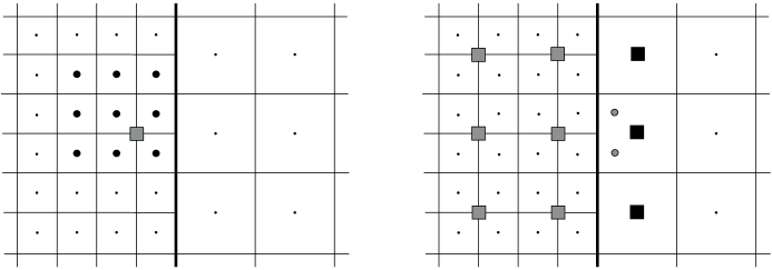
Figure 1: Guard cell filling in two spatial dimensions. In these pictures, the thick vertical line represents a refinement boundary separating fine and coarse grid regions. The picture on the left shows the first step, in which one of the parent grid cells (grey square) is filled using quadratic interpolation across nine interior fine grid cells (black circles). The other parent grid cells are filled using corresponding stencils of nine interior fine grid cells. (The asymmetry in the left panel is drawn with the assumption that the fine block’s center is toward the top-left of the panel.) The picture on the right shows the second step in which two fine grid guard cells (grey circles) are filled using quadratic interpolation across nine parent grid values (squares). These parent grid values include one layer of guard cells (black squares) obtained from the coarse grid region to the right of the interface, and two layers of interior cells (grey squares). The final step in guard cell filling (not shown in this figure) is to use “derivative matching” to fill the guard cells for the coarse grid.

The first step is a restriction operation in which interior fine grid cells are used to fill the interior grid cells of the underlying “parent” grid. The parent grid is a grid that covers the same domain as the fine grid but has twice the grid spacing. The restriction operation is depicted for the case of two spatial dimensions in the left panel of Fig. 1.

The restriction proceeds as a succession of one–dimensional quadratic interpolations, and is accurate to third order in the grid spacing. Note that the 3-cell-wide fine grid stencil used for this step (nine black circles in the figure) cannot be centered on the parent cell (grey square). In each dimension the stencil includes two fine grid cells on one side of the parent cell and one fine grid cell on the other. The stencil is always positioned so that its center is shifted toward the center of the block (assumed in the figure to be toward the upper left). This ensures that only interior fine grid points, and no fine grid guard cells, are used in this first step.

For the second step, the fine grid guard cells are filled by prolongation from the parent grid. Before the prolongation, the parent grid gets its own guard cells (black squares in the right panel of Fig. 1) from the neighboring grids of the same refinement level, in this case from the coarse grid. The stencil used in the prolongation operation is shown in the right panel of Fig. 1. The prolongation operation proceeds as a succession of one–dimensional quadratic interpolations, and is third order accurate. In this case, the parent grid stencil includes a layer of guard cells (black squares), as well as its own interior grid points (grey squares). At the end of this second step the fine grid guard cells are filled to third order accuracy.

The third step in guard cell filling is “derivative matching” at the interface. With derivative matching the coarse grid guard cell values are computed so that the first derivatives at the interface, as computed on the coarse grid, match the first derivatives at the interface as computed on the fine grid. The first derivative on the coarse grid is obtained from standard second order differencing using a guard cell and its neighbor across the interface. The first derivatives on the fine grid are computed using guard cells and their neighbors across the interface, appropriately averaged to align with the coarse grid cell centers. This third step fills the coarse grid guard cells to third order accuracy.

An alternative to derivative matching, which we do not use, is to fill the coarse grid guard cells from the first layer of interior cells of the parent grid. However, we find that such a scheme leads to unacceptably large reflection and transmission errors for waves passing through the interface. These errors are suppressed by derivative matching.

Why should third order guard cell filling be adequate to maintain overall second order accuracy? This is a nontrivial question, and there are certain subtleties that arise in our black hole evolutions. In Appendix A, we present a detailed error analysis for our guard cell filling algorithm based on simplified model equations for a scalar field in 1-D. This toy model shares many of the features of the full BSSN system and provides a useful guide to understanding the behavior of our black hole evolutions. We demonstrate that, with this algorithm, second spatial derivatives of the BSSN variables defined by Eqs. (1) acquire first order errors at grid points adjacent to mesh refinement boundaries. These first order errors show up as spikes in a convergence plot for quantities that depend on second spatial derivatives, such as the Hamiltonian constraint. The key result of this analysis, however, is a demonstration that the first order errors in second derivatives do not spoil the overall second order convergence of the evolved variables in Eqs. (1), in spite of the fact that second spatial derivatives appear on the right-hand sides of the evolution equations (2); cf. Chesshire and Henshaw (1990); Henshaw and Schwendeman (2003).

IV Black Hole Evolutions

Black hole spacetimes are a particularly challenging subject for numerical study. Astrophysical applications will require that our FMR implementation perform robustly under the adverse conditions which arise in black hole simulations, such as strong time-dependent potentials and propagating signals that become gravitational waves. In this section we demonstrate that our techniques perform convergently and accurately in the presence of strong field dynamics and singular “punctures” associated with black hole evolutions, and that these methods can be stable on the timescales required for interesting simulations.

The puncture approach to black hole spacetimes generalizes the Brill-Lindquist Brill and Lindquist (1963) prescription of initial data for black holes at rest. In this approach, the spacetime is sliced in such a way as to avoid intersecting the black hole singularity, and the spatial slices are topologically isomorphic to $\mathbf{R}^{3}$ minus one point, a puncture, for each hole. The punctures represent an inner asymptotic region of the slice which can be conformally transformed to data which are regular on $\mathbf{R}^{3}$. In this way a resting black hole of mass $M$ located at $r=0$ is expressed in isotropic spatial coordinates by $\gamma_{ij}=\Psi^{4}_{BL}\delta_{ij}$, with conformal factor $\Psi_{BL}=1+{M}/{2r}$ and $K_{ij}=0$. A direct generalization of this expression for the conformal factor can be used to represent multiple black hole punctures, and data for spinning and moving black holes can be constructed according to the Bowen-York Bowen and York (1980) prescription.

A key characteristic which makes this representation appropriate for spacetime simulations is that with suitable conditions on the regularity of the lapse and shift, the evolution equations imply that time derivatives of the data at the puncture are regular everywhere despite the blow up in $\Psi_{BL}$ at the puncture. Numerically, we treat the punctures by a prescription similar to that given in Alcubierre et al. (2003). In the BSSN formulation, this amounts to a splitting of the conformal factor $\exp({4\phi})$ into a regular part, $\exp({4\phi_{r}})$, and non-evolving singular part, $\exp({4\phi_{s}})$, given by $\Psi_{BL}$. The numerical grid is staggered to make sure the puncture does not fall directly on a grid point, and to avoid the large finite differencing error, the derivatives of $\phi_{s}$ are specified analytically.

We study two test problems, each representing a Schwarzschild black hole in a different coordinate system. Both problems test the performance of our FMR interfaces under the condition that strong-field spacetime features pass through the interfaces. The first case, described in Sec. IV.1, is a black hole in geodesic coordinates, in which the data evolve as the slice quickly advances into the singularity. In Appendix B, we present an analytic solution for the development of this spacetime with which we can compare for a direct test of the simulation. Our next test, in Sec. IV.2, uses a variant of the “1+log” slicing condition to define the lapse, $\alpha$, with vanishing shift, $\beta^{i}=0$. This gauge choice allows the slice to avoid running into the singularity, but causes the black hole to appear to grow in coordinate space so that the horizon passes though our FMR interfaces.

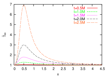
Figure 2: Evolution of the conformal metric component $\tilde{\gamma}_{xx}$, for a geodesically sliced puncture, shown at $t=0.5$, 1.0, 1.5, 2.0, and $2.5M$.

IV.1 Geodesic Slicing

We begin with the numerical evolution of a single puncture black hole using geodesic slicing.

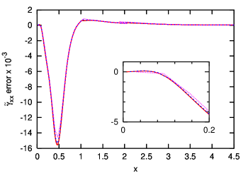
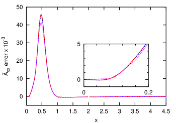
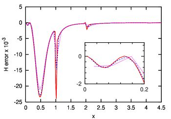
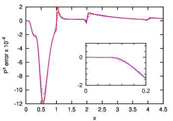
Figure 3: Convergence of the errors (numerical values minus analytic values) in $\tilde{\gamma}_{xx}$, $\tilde{A}_{xx}$, the Hamiltonian constraint $H$, and the momentum constraint $P^{x}$, for a geodesically sliced puncture along the $x$-axis, all at the time $t=2.5M$. The solid line shows the errors for the highest resolution run. The errors for the medium resolution run (dashed line) and the lowest resolution run (dotted line) have been divided by factors of 4 and 16, respectively, to demonstrate second order convergence. Note that the full domain of the simulation extends to $128M$.

As explained in Appendix B, at $t=\pi M$ the slice $\Sigma_{\pi}$ on which our data resides will reach the physical singularity; because we are not performing any excision, this sets the maximum duration of our evolution. Nevertheless, $t\approx 3M$ is long enough to test the relevant features of FMR evolution and provide us with a simple analytical solution.

In these simulations we locate the puncture black hole at the origin. The spherical symmetry of the problem allows us to restrict the simulation to an octant domain with symmetry boundary conditions, thereby saving memory and computational time. The outer boundaries are planes of constant $x$, $y$, or $z$ at $128M$ each. As noted before, one of the important uses of FMR is to enable the outer boundary to be very far from the origin, at $\gtrsim 100M$. In this case we can apply our exact solution as the outer boundary condition, though any numerical effects produced at this distant boundary are completely irrelevant for the most interesting strong-field region.

In this test we are mainly interested in how the FMR boundaries behave near the puncture and under strong gravitational fields. Even with the outer boundary far away we can, by applying multiple nested refinement regions, highly resolve the region near the puncture, as is required to demonstrate numerical convergence. To achieve the desired resolution near the puncture, we use 8 cubical refinement levels, locating the refinement boundaries at the planes $64M$, $32M$, $16M$, $8M$, $4M$, $2M$ and $1M$ in the $x$-, $y$-, and $z$-directions.

To test convergence we will examine the results of three runs with identical FMR grid structures, but different resolutions. The lowest resolution run has gridpoints $\Delta x_{f}=\Delta y_{f}=\Delta z_{f}=M/16$ apart in the finest refinement region near the puncture. The medium resolution run has double the resolution of the first run in each refinement region. The highest resolution run has twice the resolution of the medium resolution run, for a maximum resolution of $\Delta x_{f}=M/64$ near the puncture. The memory demand and computational load per timestep for the low, medium, and high resolution runs are similar to unigrid runs of $32^{3}$, $64^{3}$ and $128^{3}$ gridpoints.

Since the data in our simulations are defined at the centers of the spatial grid cells (see Fig. 1), we must interpolate when extracting data on cuts through the simulation volume. We use cubic interpolation, which is accurate to order $\Delta x^{4}$, to insure that the interpolation errors are smaller than the largest differencing errors of order $\Delta x^{2}$ expected in the simulations; cf. the discussion on post-processing in M. W. Choptuik (1992). When interpolating at a location near a refinement boundary, we adjust the stencil so that the interpolation involves only data points at the same level of refinement while still maintaining order $\Delta x^{4}$ errors.

In Fig. 2 we plot the conformal metric component $\tilde{\gamma}_{xx}$ for the highest resolution run along the $x$-axis at times $t=0.5$, 1.0, 1.5, 2.0, and $2.5M$. Note that in these coordinates the event horizon is at $r=0.5M$ at $t=0$ and moving outward toward larger values of the radial coordinate. By $t=\pi M$, the singularity is at coordinate position $r=0.5M$, so the mesh refinement interface at $x=1M$ is truly in the strong field regime. Because the slice will hit the singularity at coordinate position $x=0.5M$, the metric grows sharply there as the simulation time advances.

In the present context though, we are not so much interested in the field values of this well-studied spacetime, as in the simulation errors, that is, the differences between the analytical solution presented in Appendix B and the numerical results. These differences allow us to directly measure the errors in our numerical simulation. At late times, these errors are, not surprisingly, dominated by finite differencing errors in the vicinity of the developing singularity.

The plots in Fig. 3 compare these errors along the $x$-axis at $t=2.5M$ for the three different resolution runs described above, demonstrating the convergence of $\tilde{\gamma}_{xx}$, $\tilde{A}_{xx}$, the Hamiltonian constraint, and the $x$-component of the momentum constraint. In each panel, the solid line shows the errors for the high resolution run. The errors for the medium (dashed line) and low (dotted line) resolution runs have been divided by 4 and 16, respectively. That the curves shown lie nearly atop one another is an indication of second order convergence, i.e. that the lowest order error term depends quadratically on the gridspacing, $\Delta x$. That the remaining difference between the adjusted curves near $x=0.5M$ seems also to decrease quadratically is an indication that the next significant error term is of order $\Delta x^{4}$. We achieve convergence to the analytic solution everywhere, from very near $x=0$, through the peak region which is approaching the singularity, and in the weak field region. Animations of these results can be found in the APS auxiliary archive EPAPS; see Fig. 3A and the associated animation file in Ref. EPAPS-FMR .

Our particular interest is in the region near the refinement interfaces. Fig. 4 shows a

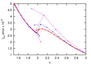
Figure 4: Close-up of the convergence of the error (numerical value minus analytic value) in $\tilde{\gamma}_{xx}$, for a geodesically sliced puncture, at $t=2.5M$, in the vicinity of the refinement boundary at $x=2M$. The errors for the high resolution run are shown by the solid line; the errors for the medium (dashed line) and low (dotted line) resolution runs have been divided by factors of 4 and 16, respectively. In this plot, we also show the location of the data points, including guardcells, using filled circles.

close-up of $\tilde{\gamma}_{xx}$ near the refinement boundary at $x=2M$. In this figure we have included the values of the guardcells used for defining finite-difference stencils near the interface. Again, the curves lie nearly atop one another, indicating second order convergence.

A similar close-up of the Hamiltonian constraint $H$ requires a little more explanation. Eq. (3a) involves up to second derivatives of the BSSN data, implemented by finite differencing. Fig. 5 shows the

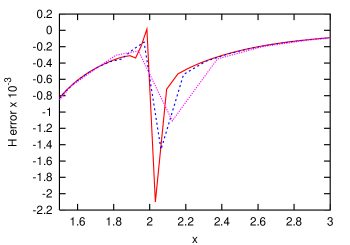
Figure 5: A view of the Hamiltonian constraint in the neighborhood of the FMR interface at $x=2M$. The errors for the high resolution run are shown by the solid line; the errors for the medium (dashed line) and low (dotted line) resolution runs have been divided by factors of 4 and 16, respectively. As discussed in the text, data points nearest to the interface converge at one order lower than in the rest of the domain.

computed values of the Hamiltonian constraint in the vicinity of the refinement boundary at $x=2M$. While the result is second-order convergent at any specific physical point in the neighborhood of the boundary, the figure indicates that the sequence of values computed at the nearest point approaching the interface as $\Delta x\rightarrow 0$ approaches zero at only first order. This is as expected according to the discussion in Appendix A (cf. Fig. 12) for a derived quantity involving second derivatives. We have specifically verified that, as with $\tilde{\gamma}_{xx}$, all BSSN variables converge to second order at the refinement boundaries.

We also examined the simulation data along cuts away from the $x$-axis and have found them to be qualitatively similar to those on the axis. In particular, plots and animations of the errors along the line $y=z=0.25M$ can be found in the EPAPS supplement; see Fig. 3B and the associated animation file in Ref. EPAPS-FMR . This particular 1-D cut is instructive since it includes the strong field region yet has no particular symmetric relation to the solution. The fact that the errors along this line are qualitatively similar to those along the $x$-axis gives us confidence that the results we display in Fig. 3 are not subject to accidental cancellations due to octant symmetry boundary conditions that might produce artificially small errors.

We have also examined the $L_{1}$ and $L_{2}$ norms of the errors in basic variables and constraints to assess the overall properties of the simulation. Representative results are shown in Fig. 6, where the top panel displays the convergence behavior of the $L_{2}$ norm of of the error in $\tilde{\gamma}_{xx}$ and the bottom panel the convergence of the $L_{2}$ norm of $H$. The errors for the medium (dashed line) and low (dotted line) resolution runs have been divided by 4 and 16, respectively. These curves lie nearly atop the errors for the high resolution run (solid line), indicating the second order convergence of these error norms; see Appendix C and Eqs. (31) and (32).

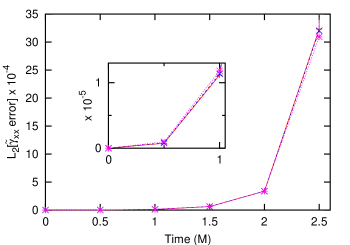
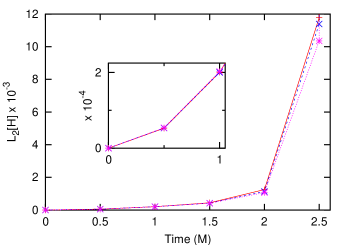
Figure 6: Convergence of the $L_{2}$ norms of the errors in $\tilde{\gamma}_{xx}$ and the Hamiltonian constraint $H$ for a geodesically sliced puncture. The numerical data points are here marked with the symbol “x”. The solid lines show the errors for the highest resolution run. The errors for the medium resolution run (dashed lines) and the lowest resolution run (dotted lines) have been divided by factors of 4 and 16, respectively, to demonstrate second order convergence.

IV.2 1 + log slicing

Having rigorously tested the code against an analytic solution, we now use a different coordinate condition to study a longer-lived run with nontrivial, nonlinear dynamical behavior in the region of FMR interface boundaries. For this purpose, we again use zero shift but with a modified “1+log” slicing condition given by

$$\frac{\partial\alpha}{\partial t}=-2\alpha\Psi_{BL}^{4}K,$$ (8)

where insertion of the factor $\Psi_{BL}=1+{M}/{2r}$, originally recommended by Alcubierre et al. (2003), has proven to enhance convergence near the puncture in our simulations. For the numerical experiments with 1+log slicing, the grid structure, including the locations of the mesh refinement interfaces, is the same as in the geodesic slicing case. We carry out three runs, with low, medium and high resolution defined as before.

A 1+log evolution serves as an excellent numerical experiment to test the robustness of our mesh refinement interfaces. The 1+log family has been well-studied in unigrid runs in the past, so the generic behavior of this coordinate system is known and provides a general context for comparison with our mesh refinement results. Because the 1+log slicing is singularity avoiding, in contrast to the geodesic slicing case, simulations in a 1+log gauge are known to last $\sim 30M-40M$, giving us an opportunity to study the properties of our mesh refinement interfaces in longer duration runs. Finally, as shown by Fig. 7, as the lapse (right panel of the figure)

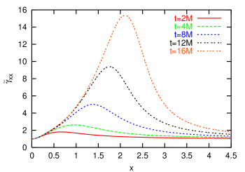
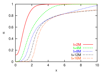
Figure 7: A time evolution sequence for the conformal metric $\tilde{\gamma}_{xx}$ and the lapse $\alpha$ using the variant of 1+log slicing given in Eq. (8). Results are shown for the highest resolution run.

collapses around the singularity, a strong gradient region in the metric (left panel of the figure) moves outward, passing through mesh refinement boundaries in the process. According to unigrid runs already in the literature (e.g., Alcubierre et al. (2003)) choosing an appropriate shift, such as the Gamma-driver shift, would cause the evolution to freeze, preventing catastrophic growth in the metric functions and confining the strong field behavior to the region $r<10M$. This also increases the stable evolution time of the simulations. For our purposes here, however, we choose to let the strong gradient region move outward because we specifically wish to study how well the mesh refinement interfaces handle a strong dynamical potential on timescales $t>10M$. We consider this an important test, since such phenomena may develop near refinement boundaries in the course of realistic astrophysical simulations of multiple black holes.

Having made this choice, we expect to see exactly what appears in Fig. 7. The metric function $\tilde{\gamma}_{xx}$ (left panel) grows due to well-understood grid stretching related to the collapse of the lapse (right panel) and the fact that grid points are falling into the black hole. The peak of the metric simultaneously moves to larger coordinate position. We expect, therefore, that at some point certain regions of the simulations will no longer exhibit second order convergence because the gradients in the metric simply grow too large, because the peak of the metric moves into a region of lower refinement that cannot resolve the gradients already present in the metric at that point, or because of a combination of the two. The simulations in this gauge, nonetheless, remain second order convergent long enough for us to study the effects of the strong potential passing through the innermost mesh refinement interfaces.

Because we do not have an analytic solution for the 1+log case to use in our convergence tests, we show three-point convergence plots instead. Specifically, for a given field $f$, we plot $(f_{\mathrm{low}}-f_{\mathrm{med}})/4$ using a dashed line and $f_{\mathrm{med}}-f_{\mathrm{high}}$ using a solid line. Since the three different resolutions “low”, “medium”, and “high” are related to each other by factors of two, the two lines in each panel should overlay exactly for perfect second order convergence.

Fig. 8 shows such a three-point convergence plot for $\tilde{\gamma}_{xx}$ and $\tilde{A}_{xx}$ for a 1-D cut along the $x$-axis.

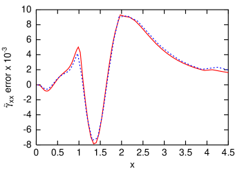
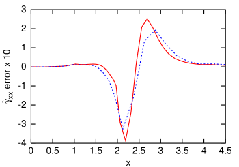
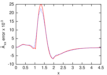
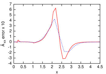
Figure 8: Three-point convergence plots for the BSSN variables $\tilde{\gamma}_{xx}$ and $\tilde{A}_{xx}$ along the $x$-axis in the 1+log slicing runs at times $t=8M$ (left panels) and $t=16M$ (right panels). For a given field $f$, the dashed line shows $(f_{\mathrm{low}}-f_{\mathrm{med}})/4$ and the solid line shows $f_{\mathrm{med}}-f_{\mathrm{high}}$.

The left panels, showing data from $t=8M$, demonstrate that the metric and other variables are second order convergent everywhere at that time. Overall, we continue to see second order convergence in the evolved variables, constraints, and norms until $t\sim 10M$.

The convergent behavior starts to break down around $t\sim 10M$ due to difficulties with resolving the sharp feature in the metric. In the region $1M\leq x\leq 2M$, between the first and second FMR boundaries, the peak itself grows sharply and the coarser grid is not sufficient to provide the resolution needed for convergent behavior. For $2M\leq x\leq 4M$, the grid is again coarsened by a factor of 2 and is not able to resolve adequately the steep gradient on the leading edge of the metric peak. A snapshot at $t=16M$ is shown in the right panels of Fig. 8; by this time, the peak of the metric has passed through two refinement interfaces (at $x=1M$ and $x=2M$). The time development of these errors, and in particular their departure from second order convergence, can be seen in the animations available in the EPAPS supplement; see Fig. 8A and the associated animation file in Ref. EPAPS-FMR .

Throughout the duration of the runs the region $x\gtrsim 5$ does remain second order convergent, even though the grid is further coarsened by factors of two at $x=8M$, $16M$, $32M$, and $64M$, since all the fields change very slowly as they approach the asymptotically flat regime. The simulations will continue to run stably past this point (to approximately $t\approx 35M$), but the resolution in the regions to the right of the interface at $x=1M$ is not sufficient to produce convergent results, as was expected.

The Hamiltonian and momentum constraints along the $x$-axis are shown in Fig. 9. Three curves are plotted in each panel. The errors for the highest resolution run are given by the solid line. The errors for the medium (dashed line) and low (dotted line) resolution runs have been divided by factors of 4 and 16, respectively. The constraints are second order convergent in the bulk for times $t\lesssim 10M$, when the resolution is sufficient to handle the growing feature in the metric (left panels). As expected, $H$ exhibits first order convergent spikes at mesh refinement interfaces; cf. Fig. 5 and Appendix A.

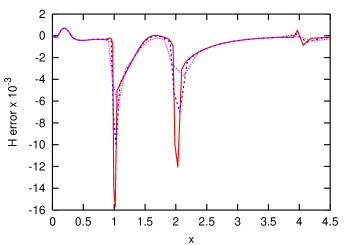
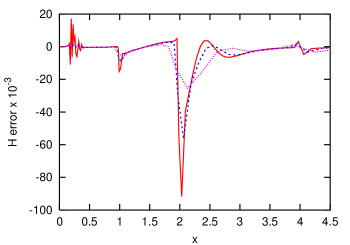
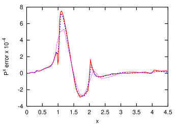
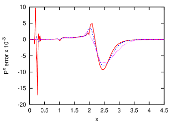
Figure 9: Convergence plots for the Hamiltonian constraint $H$ and the momentum constraint $P^{x}$ along the $x$-axis in the 1+log slicing runs at times $t=8M$ and $t=16M$. The solid lines show the errors for the high resolution run. The errors for the medium (dashed line) and low (dotted line) resolution runs have been divided by factors of 4 and 16, respectively.

For $t\gtrsim 10M$, as the peak of the fields propagates into the coarser grid regions past $x=2M$, the lowest resolutions are not sufficient to resolve the rising slope of the metric, and, like the evolved variables (Fig. 8), the constraints no longer demonstrate second order convergence. The right panels of Fig. 9 show the constraints at $t=16M$, right after the peak of the metric passes through the refinement interface at $x=2M$. See Fig. 9A and the associated animation file in Ref. EPAPS-FMR for animations of these data.

The behavior of the simulations at locations away from the $x$-axis is qualitatively similar to that shown in Figs. 8 and 9. Plots and animations of the errors along the line $y=z=0.25M$ are available in the EPAPS supplement; see Figs. 8B and 9B and their associated animation files in Ref. EPAPS-FMR .

We have also examined the $L_{1}$ and $L_{2}$ norms of the errors to assess the overall behavior of these runs, and display representative results in Fig. 10. The $L_{2}$ norms of the errors in the basic variables $\tilde{\gamma}_{xx}$ and $\tilde{A}_{xx}$ are shown in the left top and bottom panels, respectively, using 3-point convergence plots. The dashed lines show the difference between the low and medium resolution results divided by 4, and the solid lines show the difference between the medium and high resolution results, demonstrating the overall second order convergence of these simulations at early times. The $L_{1}$ norm of $H$ is displayed in the top right panel, where the solid line gives the errors for the high resolution run. The errors for the medium (dashed line) and low (dotted line) resolution runs have been divided by factors of 4 and 16, respectively to show second order convergence, as expected from Eq. (35). In the lower right panel the $L_{2}$ norm of $H$ is shown, with the solid line giving the results for the high resolution run. As discussed in Appendix C, the errors for the medium (dashed line) and low (dotted line) resolution runs have been divided by factors of $2^{3/2}$ and $4^{3/2}=8$ to account for the effects of significant first order convergent errors in $H$ at the mesh refinement boundaries, in addition to the second order convergent errors in the bulk; see Eq. (36).

One final feature of these simulations, the high frequency noise near the origin seen in the right panels of Fig. 9, requires some explanation. First of all, it is not related to the presence of the refinement boundaries; in particular, we have reproduced it in unigrid runs and with an independently-written, 1-D (spherically symmetric) code. Higher resolution exacerbates this problem: both the frequency and amplitude of the noise increase with resolution. We have found the location of this noise to be independent of resolution and the number and positions of FMR boundaries.

This feature, which we call the “point-two $M$ problem,” originates around $r\sim 0.2M$. It becomes most evident at times $t>10M$, first appearing in the lapse and $K$, which are directly coupled, and then eventually mixing into all of the extrinsic curvature variables. For the duration of the evolutions the noise remains within the region $0.0M\lesssim x\lesssim 0.5M$. Outside this region, all basic variables demonstrate satisfactory second order convergence, including at refinement boundaries, up to times $t\sim 10M$.

Having chosen a generally accepted gauge, and having focused on effects of the mesh refinement interfaces in this work, we have not fully investigated the cause of nor possible remedies for this apparent pathology. We note it here, however, as an interesting topic for future investigation.

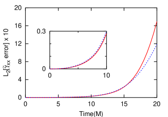
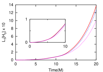
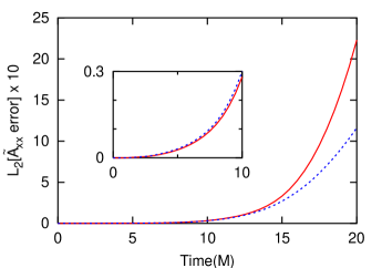
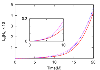
Figure 10: Convergence behavior of the $L_{1}$ and $L_{2}$ norms of the errors for the runs with 1 + log slicing. The left panel shows the $L_{2}$ norms of the errors in $\tilde{\gamma}_{xx}$ (top) and $\tilde{A}_{xx}$ (bottom), where the dashed lines show the the difference between the low and medium resolution results divided by 4, and the solid lines show the difference between the medium and high resolution results. The top right panel shows the $L_{1}$ norm of $H$, with the solid line giving the errors for the high resolution run; the errors for the medium (dashed line) and low (dotted line) resolution runs have been divided by factors of 4 and 16, respectively. The lower right panel shows the $L_{2}$ norm of $H$, with the solid line giving the results for the high resolution run. In this panel, the errors for the medium (dashed line) and low (dotted line) resolution runs have been divided by factors of $2^{3/2}$ and $4^{3/2}=8$, respectively.

V Summary

This paper demonstrates that fixed mesh refinement boundaries can be located in the strong field region of a dynamical black hole spacetime when the interface conditions are handled properly. This result was verified through simulation of a Schwarzschild black hole in geodesic coordinates, for which we have an analytic solution for comparision, and through simulations of Schwarzschild in a variation of the 1+log (singularity avoiding) slicing with zero shift. Mesh refinement technology, therefore, is a viable to way to use computational resources more efficiently, and to simulate the very large spatial domains needed to compute the dynamics of the source interactions and allow extraction of the resulting gravitational waveforms.

Our method for handling the interface conditions, based in part on the Paramesh infrastructure, is detailed. For these simulations we find that, in handling the interface condition between FMR levels, third order guard cell filling is sufficient for overall second order accuracy in the simulations. By nesting several levels of mesh refinement regions, we are able to resolve the puncture convergently while simultaneously pushing the outer boundary of our domain to $128M$ and keeping the computational problem size modest. We estimate that for only a 12% increase in the computational size of the problem, we could push the outer boundary to $256M$; moving the outer boundary out even farther will be possible for production runs on larger machines. Combined with our earlier results showing that gravitational waves pass through such FMR interfaces without significant reflections Choi et al. (2004), we have now studied, in detail, the effects of FMR interfaces on the two primary features, waves and time-varying strong potentials, of astrophysically interesting spacetimes.

In this paper, we have evolved single black holes using gauges with zero shift in order to produce test problems in which strong-field spacetime features with steep gradients pass through mesh refinement interfaces. In more realistic, astrophysical simulations of multiple black holes, we expect to use non-zero shift prescriptions. While a shift vector will allow us to control certain aspects of the dynamics, we still expect to find some strong, time-varying signals to propagate across mesh refinement boundaries. We are currently implementing non-zero shift conditions into our FMR evolutions and will report on this work in a separate publication.

Appendix A Error Analysis of Guard Cell Filling Scheme

To help pave the way for understanding the behavior of our black hole evolutions near mesh refinement boundaries, we provide here a detailed analysis of a toy model for a scalar field in one spatial dimension, using the same third order guard cell filling algorithm detailed in Sec. III. The model equations are

$$\dot{\psi} = \pi\$$ (9a)

$$\dot{\pi} = \psi^{\prime\prime}\ ,$$ (9b)

where the dot denotes a time derivative and primes denote space derivatives. These equations can be solved numerically using the same twice–iterated Crank–Nicholson algorithm used to evolve our black hole spacetimes. The fields at timestep $n+1$ are given in terms of the fields at timestep $n$ by

$$\psi^{n+1}_{j} = \psi^{n}_{j}+{\Delta t}\,\pi^{n}_{j}+\frac{\Delta t^{2}}{2}D^{2}\psi^{n}_{j}+\frac{\Delta t^{3}}{4}D^{2}\pi^{n}_{j}\$$ (10a)

$$\pi^{n+1}_{j} = \pi^{n}_{j}+{\Delta t}\,D^{2}\psi^{n}_{j}+\frac{\Delta t^{2}}{2}D^{2}\pi^{n}_{j}+\frac{\Delta t^{3}}{4}D^{4}\psi^{n}_{j}\quad$$ (10b)

where $D^{2}$ is a finite difference operator approximating the second spatial derivative, and $D^{4}=(D^{2})^{2}$.

Consider for the moment a uniform spatial grid. If $D^{2}$ is the usual second order accurate centered difference operator, the dominant source of error for $\psi^{n+1}_{j}$ comes from the term proportional to $\Delta t^{3}$. This term has the wrong numerical coefficient as compared to the Taylor series expansion of the exact solution. The dominant sources of error for $\pi^{n+1}_{j}$ come from the term proportional to $\Delta t^{3}$, which also has the wrong numerical coefficient, and from the second order error in $D^{2}\psi^{n}_{j}$. For a uniform grid the dominant error in $D^{2}\psi^{n}_{j}$ is $D^{4}\psi^{n}_{j}\,\Delta x^{2}/12$, so the leading errors for a single timestep are

$$(\psi^{n+1}_{j})_{err} = \frac{1}{12}\Delta t^{3}D^{2}\pi^{n}_{j}\$$ (11a)

$$(\pi^{n+1}_{j})_{err} = \frac{1}{12}\Delta t\,(\Delta t^{2}+\Delta x^{2})D^{4}\psi^{n}_{j}\ .$$ (11b)

For $\Delta t\sim\Delta x$, each of these one–time–step errors is proportional to $\Delta x^{3}$. If we evolve the initial data to a finite time $T$, the ${\cal O}(\Delta x^{3})$ errors accumulate over $N=T/\Delta t$ timesteps resulting in second order errors. Thus, the basic variables $\psi$ and $\pi$ are second order convergent on a uniform grid.

On a non–uniform grid, guard cell filling introduces errors of order $\Delta x^{3}$ in $\psi$ at grid points adjacent to the boundary. This leads to errors of order $\Delta x$ in $D^{2}\psi^{n}_{j}$ and $1/\Delta x$ in $D^{4}\psi^{n}_{j}$. From Eq. (10b) we see that in one timestep $\pi$ can acquire errors of order $\Delta x^{2}$. The concern is that these errors might accumulate over $N=T/\Delta t$ timesteps to yield first order errors. This, in fact, does not happen. Simple numerical experiments show that $\psi$ and $\pi$ are second order convergent on a non–uniform grid with third order guard cell filling.

We can understand this result with the following heuristic reasoning. The numerical algorithm of Eq. (10) approximates, as does any mathematically sound numerical scheme, the exact solution of the scalar field equations (Eq. (9)) in which the field $\pi$ propagates along the light cone. The “bulk” errors displayed in Eq. (11b) accumulate along the past light cone to produce an overall error of order $N\,\Delta x^{3}\sim\Delta x^{2}$ at each spacetime point. Errors in guard cell filling, which occur at a fixed spatial location, do not accumulate over multiple timesteps since the past light cone of a given spacetime point will cross the interface (typically) no more than once.

The characteristic fields for the system (9) are $\pi\pm\psi^{\prime}$ so that $\psi^{\prime}$, like $\pi$, propagates along the light cone. As a result, the value of $\psi$ at a given spacetime point is determined by data from the interior of the past light cone. From Eq. (10a) we see that the one–time–step errors for $\psi$ due to guard cell filling are order $\Delta x^{3}$. These errors can accumulate over $N$ timesteps to yield errors of order $N\,\Delta x^{3}\sim\Delta x^{2}$.

The derivatives $\psi^{\prime}$ and $\psi^{\prime\prime}$ are computed at finite time $T$ by evolving the $\psi$, $\pi$ system for $T/\Delta t$ timesteps then taking the centered, second order accurate numerical derivatives of $\psi$. Numerical experiments show that $\psi^{\prime}$ and $\psi^{\prime\prime}$, defined in this way, are second order convergent on a non–uniform grid with third order guard cell filling. Continuing with our heuristic discussion, we can understand the second order convergence of $\psi^{\prime\prime}$ as follows. Let $(\psi^{n}_{j})_{err}\approx E^{n}_{j}\Delta x^{2}$ denote the error in $\psi$ at grid point $n$, $j$, where the coefficient $E^{n}_{j}$ is independent of $\Delta x$. Some of this error is due to guard cell filling at the mesh refinement interface and some is due to the accumulation of “bulk” errors (11). Now, the second derivative of $\psi$, computed as $D^{2}\psi^{n}_{j}=(\psi^{n}_{j+1}-2\psi^{n}_{j}+\psi^{n}_{j-1})/{\Delta x}^{2}$, will contain errors of the form $(D^{2}\psi^{n}_{j})_{err}=E^{n}_{j+1}-2E^{n}_{j}+E^{n}_{j-1}$. Since the bulk errors are smooth, the bulk contribution to $E^{n}_{j+1}-2E^{n}_{j}+E^{n}_{j-1}$ will scale as $\Delta x^{2}$. It is also the case that the errors due to guard cell filling are smooth. This is because the value of $\psi$ at any given point is determined by the interior of the past light cone, so its error includes an accumulation of guard cell filling errors along the history of the mesh refinement interface. In the limit of high resolution this accumulation of error approaches the same value at neighboring grid points $j-1$, $j$, and $j+1$. In other words, the guard cell filling contribution to $E^{n}_{j+1}-2E^{n}_{j}+E^{n}_{j-1}$ approaches zero as $\Delta x\to 0$. Evidently, the guard cell filling contribution, like the bulk contribution, scales like $\Delta x^{2}$.

The discussion above indicates that we can evolve the scalar field system of Eq. (9) for a finite time on a grid with mesh refinement, numerically compute the second derivative of $\psi$, and find that $\psi^{\prime\prime}$ is second order accurate. Without shift, the BSSN equations (2c) and (2d) are similar to the scalar field equations with $\tilde{\gamma}_{ij}$ playing the role of $\psi$ and $-\tilde{A}_{ij}$ playing the role of $\pi$. This feature was one of the original motivations behind the BSSN system. Note that the term analogous to $\psi^{\prime\prime}$ in the $\dot{\pi}$ equation is the term $\tilde{\gamma}^{lm}\tilde{\gamma}_{ij,lm}$ contained in the trace–free part of the Ricci tensor, which appears on the right–hand side of Eq. (2d). Obviously there are many other terms that appear on the right–hand side of the $d\tilde{A}_{ij}/dt$ equation. We can model the effect of these terms by including a fixed function on the right–hand side of the $\dot{\pi}$ equation:

$$\dot{\psi} = \pi\$$ (12a)

$$\dot{\pi} = \psi^{\prime\prime}-\chi^{\prime\prime}\ .$$ (12b)

We have written the fixed function as the second derivative of $\chi$. For simplicity we choose $\chi$ to depend on $x$ only, the most relevant dependence for our consideration of behavior across spatial resolution interfaces. The general solution of this system is then

$$\psi(t,x) = \bar{\psi}(t,x)+\chi(x)\$$ (13a)

$$\pi(t,x) = \bar{\pi}(t,x)\$$ (13b)

where $\bar{\psi}$, $\bar{\pi}$ is a solution of the homogeneous wave equation (Eq. (9)).

The extended model system of Eq. (12) can be solved numerically with the discretization

$$\psi^{n+1}_{j} = \psi^{n}_{j}+{\Delta t}\,\pi^{n}_{j}+\ldots\$$ (14a)

$$\pi^{n+1}_{j} = \pi^{n}_{j}+{\Delta t}\,(D^{2}\psi^{n}_{j}-D^{2}\chi_{j})+\ldots\$$ (14b)

The higher order terms in $\Delta t$, not shown here, come from the iterations in our iterated Crank–Nicholson algorithm. It is important to recognize that the $\chi^{\prime\prime}$ term is expressed as the numerical second derivative of $\chi_{j}$ and not as the discretization of the analytical second derivative, $(\chi^{\prime\prime})_{j}$. The reason for this choice is that $D^{2}\chi_{j}$ mimics the effect of the extra terms on the right–hand side of Eq. (2d) which, in our BSSN code, depend on the discrete first and second derivatives of the BSSN variables $\phi$ and $\tilde{\Gamma}^{i}$.

From the discussion of the wave equation (Eq. (9)) we can anticipate the results of numerical experiments with the model system (Eq. (12)) on a non–uniform grid. For arbitrary initial data $\psi^{0}_{j}$, $\pi^{0}_{j}$, the numerical solution is given by

$$\psi^{n}_{j} = \bar{\psi}^{n}_{j}+\chi_{j}\$$ (15a)

$$\pi^{n}_{j} = \bar{\pi}^{n}_{j}\$$ (15b)

where $\bar{\psi}^{n}_{j}$, $\bar{\pi}^{n}_{j}$ is the numerical solution of the homogeneous wave equation (Eq. (9)) with initial data $\bar{\psi}^{0}_{j}-\chi_{j}$, $\bar{\pi}^{0}_{j}$. The order of convergence for $\psi^{n}_{j}$ is determined by how rapidly, as $\Delta x\to 0$, the numerical solution in Eq. (15a) approaches the exact solution $\psi(t,x)=\bar{\psi}(t,x)+\chi(x)$. Since $\chi_{j}$ is simply the projection of the analytic function $\chi(x)$ onto the numerical grid, the term $\chi_{j}$ in the numerical solution (Eq. (15a)) does not contribute any error. We have already determined that on a non–uniform grid $\bar{\psi}^{n}_{j}$ approaches $\bar{\psi}(t,x)$ with second order accuracy. Thus, we expect $\psi^{n}_{j}$ to be second order convergent.

What about derivatives of $\psi$? The order of convergence for $D^{1}\psi^{n}_{j}$ is found by comparing the discrete derivative $D^{1}\psi^{n}_{j}=D^{1}\bar{\psi}^{n}_{j}+D^{1}\chi_{j}$ to the analytic solution $\psi^{\prime}=\bar{\psi}^{\prime}+\chi^{\prime}$. Again, as we have discussed, $D^{1}\bar{\psi}^{n}_{j}$ approaches $\bar{\psi}^{\prime}$ with second order errors. It is also easy to see that the numerical derivative $D^{1}\chi_{j}$ approaches $\chi^{\prime}$ with second order accuracy. Away from grid interfaces this is obviously true, assuming that $D^{1}$ is the standard second order accurate centered difference operator. For points adjacent to a grid interface, guard cell values for $\psi$ are filled with third order errors. These errors lead to second order errors in $D^{1}\psi^{n}_{j}$. Overall then, we expect second order convergence for $D^{1}\psi^{n}_{j}$.

The expected convergence rates for $\psi$ and $\psi^{\prime}$ are confirmed by the results shown in Fig. 11. For these numerical tests, we chose $\chi(x)=\exp((x-50)/10)$ and initial data

$$\psi(0,x) = 100e^{-(x+10)^{2}/400}+e^{(x-50)/10}\$$ (16a)

$$\pi(0,x) = \frac{1}{2}(x+10)e^{-(x+10)^{2}/400}\ .$$ (16b)

Each set of curves shows the errors at three different resolutions, $\Delta x=5/16$, $5/32$, and $5/64$, where $\Delta x$ is the fine grid spacing. The evolution time is $20.83$, corresponding to $200$, $400$, or $800$ timesteps (depending on the resolution) and a Courant factor of $1/3$.

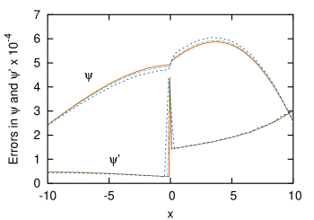
Figure 11: Convergence tests for $\psi$ and $\psi^{\prime}$. The mesh interface is at $x=0$, with the fine grid on the left and coarse grid on the right. The errors in $\psi$ and $\psi^{\prime}$ for the high resolution case are shown by the solid line. The errors are divided by factors of 4 and 16 for the middle (dashed line) and low (dotted line) resolution cases, respectively.

The order of convergence for the second derivative of $\psi$ is determined from a comparison of $D^{2}\psi^{n}_{j}=D^{2}\bar{\psi}^{n}_{j}+D^{2}\chi_{j}$ and the analytic solution $\psi^{\prime\prime}=\bar{\psi}^{\prime\prime}+\chi^{\prime\prime}$. We have seen that $D^{2}\bar{\psi}^{n}_{j}$ approaches $\bar{\psi}^{\prime\prime}$ with second order accuracy. The situation for $D^{2}\chi_{j}$, however, is somewhat different. Away from any grid interface $D^{2}\chi_{j}$ will approach $\chi^{\prime\prime}$ with second order accuracy, assuming $D^{2}$ is the standard second order accurate finite difference operator. But for points adjacent to the interface, and only those points, guard cell filling errors of order $\Delta x^{3}$ in $\chi$ will lead to first order errors in $D^{2}\chi_{j}$. Thus, we expect to find second order convergence for $D^{2}\psi^{n}_{j}$ at all points except those points adjacent to the interface. Points adjacent to the interface should be first order convergent.

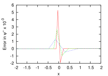
Figure 12: Convergence test for $\psi^{\prime\prime}$. The solid curve is the error in $\psi^{\prime\prime}$ for the highest resolution run. As in Fig. 11, the interface is at $x=0$ and the errors for the middle (dashed line) and low (dotted line) resolution cases are divided by factors of 4 and 16, respectively. The grid points adjacent to the interface do not coincide because $\psi^{\prime\prime}$ is only first order convergent at these points.

Fig. 12 shows the results of our convergence test for $\psi^{\prime\prime}$. The spikes at the interface ($x=0$) appear because the two grid points adjacent to the interface are only first order convergent. Elsewhere, the plot shows second order convergence.

The behavior demonstrated in Fig. 12 also occurs in the BSSN system when we examine the convergence plot for the Hamiltonian constraint. In graphing the Hamiltonian constraint $H$, we are comparing a combination of grid functions that includes second derivatives of the BSSN variables to the exact analytical solution for $H$, namely, zero. We therefore expect spikes to appear at interfaces in the convergence plot for the Hamiltonian constraint, and indeed they do (see, for example, Figs. 3 and 9).

We wish to emphasize that the lack of second order convergence for second spatial derivatives at grid points adjacent to the interfaces is not due to any error in our code, or shortcoming of the numerical algorithm. Since the undifferentiated variables are second order convergent everywhere, we can always assure second order convergence of their derivatives by using suitable finite difference stencils. For example, in computing $D^{2}\psi^{n}_{j}$ from $\psi^{n}_{j}$ we can use a second order accurate one-sided operator $D^{2}$ that avoids using guard cell values altogether. With such a choice the spikes in Fig. 12 disappear, and $D^{2}\psi^{n}_{j}$ is everywhere second order convergent. In our BSSN code, it is most convenient to compute the Hamiltonian constraint using the same centered difference operator $D^{2}$ that we use for the evolution equations. As a consequence, spikes appear at the grid interfaces in the convergence plots (Fig. 3 and 9).

Appendix B Analytic Solution for Geodesically Sliced Schwarzschild

In a numerical simulation, geodesic coordinates are obtained by using unit lapse and vanishing shift. This implies that the grid points will follow geodesic trajectories through the physical spacetime. We present here a physical derivation of the Schwarzchild spacetime metric in this well-known coordinate system, based on those geodesics; an alternate derivation is available in Refs. Misner et al. (1973); Brügmann (1996, 1999).

The Schwarzschild geometry in standard coordinates is given by

$$ds^{2}=-g_{TT}^{\mbox{ }}dT^{2}+g_{RR}dR^{2}+R^{2}d\Omega^{2},$$ (17)

where $g_{TT}=g_{RR}^{-1}=\left(1-2M/R\right)$.

To express this metric in geodesic coordinates, consider a spatial Cauchy surface $\Sigma_{0}$ in a 4-manifold $\cal{M}$ and a congruence of radial geodesics crossing $\Sigma_{0}$. Let the affine parameter $\tau$ for each geodesic be zero at $\Sigma_{0}$. Considering subsequent slices of constant proper time, we can set a global time $\tau$ which we use to define a new foliation $\Sigma_{\tau}$ of $\cal{M}$. Each geodesic in the congruence is labeled by the coordinates of its initial “starting” point in $\Sigma_{0}$. The radial position $\rho$ of the starting point in $\Sigma_{0}$ can thus be promoted to a new radial coordinate on $\cal{M}$ to pair with the time coordinate $\tau$.

Now we will derive the metric components in this $\tau$-$\rho$ coordinate system. The affine parameter $\tau$ induces the normalized vector $n^{a}=(\partial/\partial\tau)^{a}$ tangent to the geodesic, implying that the lapse $g_{\tau\tau}=-1$. Assuming the geodesics begin at rest so that $n^{a}$ is normal to $\Sigma_{0}$ implies that $g_{\tau\rho}=0$ initially. Furthermore, the geodesic equation $n^{a}\nabla_{a}n^{b}=0$ requires that $g_{\tau\rho,\tau}=0$. Thus $g_{\tau\rho}$ (the shift) must remain zero.

A straightforward transformation from Eq. (17) for the remaining metric coefficient yields

$$g_{\rho\rho}=\frac{\left(\partial R/\partial\rho\right)^{2}}{\left[\left(\partial T/\partial\tau\right)g_{TT}\right]^{2}}.$$ (18)

The term in the denominator is the energy defined for geodesics on this spacetime, and it is conserved along the geodesics: $n^{a}\nabla_{a}(n_{b}\xi^{b})=0$, where $\xi^{b}=(\partial/\partial T)^{b}$ is the timelike Killing field. On $\Sigma_{0}$ one can evaluate this energy as $\sqrt{-g^{0}_{TT}}$, where $g^{0}_{ab}=g_{ab}|_{T=0}$. This gives

$$g_{\rho\rho}=g^{0}_{RR}\left(\frac{\partial R}{\partial\rho}\right)^{2}=\left(1-\frac{2M}{\rho}\right)^{-1}\left(\frac{\partial R}{\partial\rho}\right)^{2}.$$ (19)

A similar application of conservation of energy in $n^{a}n_{a}=-1$ yields Brügmann (1996, 1999):

$$\tau-\frac{\rho^{3/2}}{(2M)^{1/2}}\left[\sqrt{\frac{R}{\rho}\left(1-\frac{R}{\rho}\right)}+\arccos\sqrt{\frac{R}{\rho}}\right]=0.$$ (20)

This expression provides an implicit definition for $R=R(\rho,\tau)$, which is easily inverted numerically to high precision.

To perform numerical evolutions the geodesic coordinates have a drawback: the physical singularity is already present on the initial slice $(\tau=0)$ at $\rho=0$. We can avoid this problem by going to isotropic coordinates $(r,\theta,\phi)$ by means of the transformation $\rho=r\left(1+{M}/{2r}\right)^{2}$. We see that $\rho\rightarrow\infty$ both as $r\rightarrow 0$ and as $r\rightarrow\infty$. For real $r$ the minimum value of $\rho$ is $\rho=2M$ (the horizon) at $r={M}/{2}$, now the surface closest to the physical singularity on the initial slice. Substituting $\rho=2M$ into Eq. (20) we see that geodesics originating on this surface reach the physical singularity, $R=0$, at time $\tau=\pi M$, defining the maximum temporal extent of our coordinate system.

Returning to the metric, the transformation to isotropic coordinates gives us

$$g_{\rho\rho}=\left(\frac{\partial R}{\partial\rho}\right)^{2}\left(1+\frac{M}{2r}\right)^{4}.$$ (21)

From Eq. (21) we can express the final metric as:

$$ds^{2}=-d\tau^{2}+\left(\frac{\partial R}{\partial\rho}\right)^{2}\left(1+\frac{M}{2r}\right)^{4}dr^{2}+R^{2}d\Omega^{2}.$$ (22)

Expressions for the extrinsic curvature, which have not previously appeared in the literature, can be derived in a similar manner. As we know from the ADM formalism York (1979); Arnowitt et al. (1962), the extrinsic curvature can be viewed as the rate of change of the spatial metric

$$K_{ab}=-\frac{1}{2}\frac{dg_{ab}}{d\tau}$$ (23)

when the lapse is unity and the shift is zero. This gives

$$K_{\rho\rho}=-\frac{1}{2}\left(1+\frac{M}{2r}\right)^{4}\frac{\partial}{\partial\tau}\left(\frac{\partial R}{\partial\rho}\right)^{2}.$$ (24)

To evaluate the partial derivatives in Eqs. (22) and (24), we note that if we have a function $f=f(u,v,w)=0$ defining $u$ as an implicit function of $v$ and $w$, we can use the chain rule and the implicit function theorem to show that

$$\frac{\partial u}{\partial v} = -\frac{\partial f/\partial v}{\partial f/\partial u}$$ (25)

$$\frac{\partial^{2}u}{\partial w\partial v} = -\left(\frac{\partial f}{\partial u}\right)^{-1}\left[\frac{\partial^{2}f}{\partial v\partial w}+\frac{\partial^{2}f}{\partial u^{2}}\frac{\partial f}{\partial v}\frac{\partial f}{\partial w}\left(\frac{\partial f}{\partial u}\right)^{-2}\right]$$ (26)

$$\mbox{}+\left(\frac{\partial f}{\partial u}\right)^{-2}\left(\frac{\partial^{2}f}{\partial v\partial u}\frac{\partial f}{\partial w}+\frac{\partial^{2}f}{\partial u\partial w}\frac{\partial f}{\partial v}\right).$$

Taking for $f$ the left hand side of Eq. (20), and, noting that $\partial f/\partial{\tau}=1$, we conclude that:

$$K_{\rho\rho} = \left(1+\frac{M}{2r}\right)^{4}\frac{\partial f}{\partial\rho}\left(\frac{\partial f}{\partial R}\right)^{-3}$$ (27)

$$\mbox{}\times\left[\frac{\partial^{2}f}{\partial\rho\partial R}-\frac{\partial^{2}f}{\partial R^{2}}\frac{\partial f}{\partial\rho}\left(\frac{\partial f}{\partial R}\right)^{-1}\right]$$

and

$$K_{\theta\theta}=R\left(\frac{\partial f}{\partial R}\right)^{-1}\qquad K_{\phi\phi}=K_{\theta\theta}\sin^{2}(\theta).$$ (28)

There are no off-diagonal terms. Observe that we have only partial derivatives of $f$ that can be obtained analytically from Eq. (20), and easily evaluated numerically.

Appendix C Definition of $L_{n}$ norms and scaling properties

For a function $f$ defined on a uniform grid $\Delta x=\Delta y=\Delta z\equiv h$, we take the $L_{n}$ norm of the function to be

$$L_{n}[f]=\left(\sum_{\rm grid}h^{3}|f_{jkm}|^{n}\right)^{1/n}$$ (29)

where $f_{jkm}$ is the value of the function at grid point $(j,k,m)$; cf. Gustafsson et al. (1995). If the function is defined on a non-uniform grid with $\ell$ refinement levels, the $L_{n}$ norm becomes

$$L_{n}[f]=\left(\sum_{\rm grid\,1}h_{1}^{3}|f_{jkm}|^{n}+\ldots+\sum_{{{\rm grid}\;\ell}}h_{2}^{3}|f_{jkm}|^{n}\right)^{1/n},$$ (30)

where $h_{i}$ is the cell size on the $i^{\rm th}$ grid. In our work, the function $f$ denotes an error, either derived from comparison with an analytic solution (for example, the Hamiltonian constraint for all our runs, and the basic variables with geodesic slicing) or from comparison with a run at a different resolution as part of a three-point convergence test (for the basic variables with 1 + log slicing).

It is useful to work out the scaling behavior expected when error norms from runs with different resolutions are compared. Recall that, for the runs presented in this paper, $h_{\rm low}=2h_{\rm med}=4h_{\rm high}$, and the errors in basic variables such as $\tilde{\gamma}_{pq}$ and $\tilde{A}_{pq}$ are expected to scale as $f\sim h^{2}$ everywhere. Let $N$ be the characteristic number of zones along one dimension of a simulation volume, so that $h\sim 1/N$. We focus on the $L_{1}$ and $L_{2}$ norms, which are the ones generally used to examine errors in numerical relativity. Then

$$L_{1}\sim\sum_{\rm grid}h^{3}f\;\sim\;N^{3}h^{3}f\;\sim f\;\sim h^{2}$$ (31)

and

$$L_{2}\sim\left(\sum_{\rm grid}h^{3}f^{2}\right)^{1/2}\sim\;f\;\sim h^{2},$$ (32)

so that both the $L_{1}$ and $L_{2}$ norms should exhibit second order convergence in this case. Note that these expressions are valid not only for unigrid runs but also for our FMR simulations, since the refinement structure of the grid is the same in all these runs.

This situation regarding the $L_{1}$ and $L_{2}$ norms of the Hamiltonian constraint $H$ is somewhat more complicated. As we have shown in Sec. IV and Appendix A, $H$ has errors that scale as $f\sim h$ on refinement boundaries and as $f\sim h^{2}$ in the bulk. For the runs with geodesic slicing, the errors in $H$ in the bulk near the puncture dominate over those at the refinement boundaries; see Fig. 3. Since these errors show second order convergence $f\sim h^{2}$, we expect that both the $L_{1}$ and $L_{2}$ norms will also scale $\sim h^{2}$, as in Eqs. (31) and (32). However, in the case of 1 + log slicing, the first order convergent errors on the refinement boundaries play a larger role; see Fig. 9. To account for this, we write

$$L_{n}\sim\left(\sum_{\rm boundary}h^{3}f^{n}+\sum_{\rm bulk}h^{3}f^{n}\right)^{1/n}.$$ (33)

The number of zones on the boundary $\sim N^{2}$ while the number of zones in the bulk $\sim N^{3}$, for sufficiently large $N$. Then

$$L_{n}\sim\left(N^{2}h^{3}h^{n}+N^{3}h^{3}h^{2n}\right)^{1/n}\sim(h^{n+1}+h^{2n})^{1/n}.$$ (34)

This gives

$$L_{1}\sim h^{2}$$ (35)

and, since $h\ll 1$,

$$L_{2}\sim h^{3/2}$$ (36)

for the scaling of the norms of $H$ in 1 + log slicing.

References

- Schutz (2003) B. Schutz, in The Astrophysics of Gravitational Wave Sources, edited by J. M. Centrella (AIP, Melville, NY, 2003).
- Choptuik (1993) M. W. Choptuik, Phys. Rev. Lett. 70, 9 (1993).
- Choptuik et al. (2003) M. W. Choptuik, E. W. Hirschmann, S. L. Liebling, and F. Pretorius, Phys. Rev. D 68, 044007 (2003), eprint gr-qc/0305003.
- Hern (1999) S. D. Hern, Ph.D. thesis, Cambridge University (1999), eprint gr-qc/0004036.
- Belanger (2001) Z. B. Belanger, Master’s thesis, Oakland University (2001).
- Brügmann (1996) B. Brügmann, Phys. Rev. D 54, 7361 (1996), eprint gr-qc/9608050.
- Brügmann (1999) B. Brügmann, Int. J. Mod. Phys. D 8, 85 (1999), eprint gr-qc/9708035.
- Schnetter et al. (2004) E. Schnetter, S. H. Hawley, and I. Hawke, Class. Quantum Grav. 21, 1465 (2004), eprint gr-qc/0310042.
- Brügmann et al. (2003) B. Brügmann, W. Tichy, and N. Jansen (2003), eprint gr-qc/0312112.
- Diener et al. (2000) P. Diener, N. Jansen, A. Khokhlov, and I. Novikov, Class. Quantum Grav. 17, 435 (2000), gr-qc/9905079.
- Brown and Lowe (February 21, 2003) D. Brown and L. Lowe, Penn State Numerical Relativity Lunch Talk (February 21, 2003), eprint gr-qc/0408089.
- Papadopoulos et al. (1998) P. Papadopoulos, E. Seidel, and L. Wild, Phys. Rev. D 58, 084002 (1998), gr-qc/9802069.
- New et al. (2000) K. C. B. New, D.-I. Choi, J. M. Centrella, P. MacNeice, M. Huq, and K. Olson, Phys. Rev. D 62, 084039 (2000), eprint gr-qc/0007045.
- Choi et al. (2004) D.-I. Choi, J. D. Brown, B. Imbiriba, J. Centrella, and P. MacNeice, J. Computat. Physics 193, 398 (2004), eprint physics/0307036.
- Shibata and Nakamura (1995) M. Shibata and T. Nakamura, Phys. Rev. D 52, 5428 (1995).
- Baumgarte and Shapiro (1999) T. W. Baumgarte and S. L. Shapiro, Phys. Rev. D 59, 024007 (1999), eprint gr-qc/9810065.
- York (1979) J. York, in Sources of Gravitational Radiation, edited by L. Smarr (Cambridge University Press, Cambridge, England, 1979).
- Alcubierre et al. (2003) M. Alcubierre, B. Brügmann, P. Diener, M. Koppitz, D. Pollney, E. Seidel, and R. Takahashi, Phys. Rev. D 67, 084023 (2003), eprint gr-qc/0206072.
- Press et al. (1986) W. H. Press, B. P. Flannery, S. A. Teukolsky, and W. T. Vetterling, Numerical Recipes (Cambridge University Press, Cambridge, England, 1986).
- Teukolsky (2000) S. Teukolsky, Phys. Rev. D 61, 087501 (2000), eprint gr-qc/9909026.
- MacNeice et al. (2000) P. MacNeice, K. Olson, C. Mobarry, R. de Fainchtein, and C. Packer, Computer Physics Comm. 126, 330 (2000).
- (22) http://ct.gsfc.nasa.gov/paramesh/Users_manual/ amr.html.
- DeZeeuw and Powell (1993) D. DeZeeuw and K. Powell, J. Computat. Phys. 104, 56 (1993).
- Dursi and Zingale (2003) L. J. Dursi and M. Zingale, in Proceedings of the 2003 Chicago AMR Workshop (2003), eprint astro-ph/0310891.
- Chesshire and Henshaw (1990) G. Chesshire and W. D. Henshaw, J. Computat. Phys. 90, 1 (1990).
- Henshaw and Schwendeman (2003) W. D. Henshaw and D. W. Schwendeman, J. Computat. Phys. 191, 420 (2003).
- Brill and Lindquist (1963) D. Brill and R. Lindquist, Phys. Rev. 131, 471 (1963).
- Bowen and York (1980) J. Bowen and J. W. York, Phys. Rev. D 21, 2047 (1980).
- M. W. Choptuik (1992) T. P. M. W. Choptuik, D. S. Goldwirth, Class. Quantum Grav. 9, 721 (1992).
- (30) EPAPS-FMR (2004), see AIP Document No. EPAPS: (to be inserted by publisher) for supplemental material, including plots of the simulation errors along the 1-D off-axis cut and animations of the simulation errors for both on-axis and off-axis cuts. This document may be retrieved via the EPAPS homepage (http://www.aip.org/pubservs/epaps.html) or from ftp.aip.org in the directory /epaps/. See the EPAPS homepage for more information.
- Misner et al. (1973) C. W. Misner, K. S. Thorne, and J. A. Wheeler, Gravitation (W. H. Freeman, San Francisco, 1973).
- Arnowitt et al. (1962) R. Arnowitt, S. Deser, and C. W. Misner, in Gravitation: An Introduction to Current Research, edited by L. Witten (John Wiley, New York, 1962), pp. 227–265.
- Gustafsson et al. (1995) B. Gustafsson, H.-O. Kreiss, and J. Oliger, Time dependent problems and difference methods (Wiley, New York, 1995).