High Resolution Calculations of Merging Neutron Stars II: Neutrino Emission

Abstract

The remnant resulting from the merger of two neutron stars produces neutrinos in copious amounts. In this paper we present the neutrino emission results obtained via Newtonian, high-resolution simulations of the coalescence event. These simulations use three-dimensional smoothed particle hydrodynamics together with a nuclear, temperature dependent equation of state and a multi-flavour neutrino leakage scheme. We present the details of our scheme, discuss the neutrino emission results from a neutron star coalescence and compare them to the core-collapse supernova case where neutrino emission has been studied for several decades. The average neutrino energies are similar to those in the supernova case, but contrary to the latter, the luminosities are dominated by electron-type antineutrinos which are produced in the hot, neutron-rich, thick disk of the merger remnant. The cooler parts of this disk contain substantial fractions of heavy nuclei, which, however, do not influence the overall neutrino emission results significantly. Our total neutrino luminosities from the merger event are considerably lower than those found in previous investigations. This has serious consequences for the ability to produce a gamma-ray burst via neutrino annihilation. The neutrinos are emitted preferentially along the initial binary rotation axis, an event seen “pole-on” would appear much brighter in neutrinos than a similar event seen “edge-on”.

1 Introduction

Binary pulsars such as the famous PSR 1913+16 are fascinating laboratories for extreme physics. Soon after its discovery it was realized that the orbit of PSR 1913+16 is decaying due to energy constantly leaking out of the system in the form of gravitational waves (Taylor 1994) and therefore making the final coalescence an inescapable consequence. This merger event holds promises for areas as diverse as gamma-ray bursts (Paczyński 1986, Eichler et al. 1989, Narayan et al. 1992), ground-based gravitational wave detection (Abramovici et al. 1992, Kuroda et al. 1997, Bradaschia et al. 1990, Danzmann 1997) and the formation of rapid neutron capture elements (Lattimer & Schramm 1974, Lattimer & Schramm 1976, Symbalisty & Schramm 1982, Eichler et al. 1989, Rosswog et al. 1999, Freiburghaus et al. 1999).
The involved physics of the event is in almost every aspect “exotic”: the neutron star fluid moves in and determines the dynamical, curved space-time; in the centers of the stars and the resulting merger remnant the baryon densities reach multiples of the nuclear saturation density, $\rho_{s}=2.5\cdot 10^{14}$ gcm^-3; nuclear reactions proceed via extremely neutron-rich and short-lived isotopes; and the initial neutron star magnetic fields are expected to be amplified during the merger to a strength, $B\sim 10^{17}$ G, so that their feed-back on the fluid flow becomes dynamically important (Thompson & Duncan 1993, Thompson 1994, Kluzniak & Ruderman 1998, Rosswog & Davies 2002).
Neutron star mergers represent a severe challenge for computer simulations. The event is genuinely multidimensional and unlike, for example, with core-collapse supernovae (SNe), there are no basic open questions that could be first addressed in restricted dimensions, as e.g. the robustness of the delayed neutrino-driven supernova mechanism. Nevertheless, the two events have several common aspects: compact objects are formed in the center of the event and huge amounts of gravitational binding energy, of order $10^{53}$ erg, are released in form of neutrinos making neutrino physics a key ingredient of both scenarios. The material in the innermost layers of both configurations is very dense, neutron rich, and neutrino opaque. Most neutrinos are radiated from a hot and thick accretion disk in the neutron star merger case, and from a shock heated mantle in the standard supernova scenario. The neutrino emission and absorption are the key features in the picture of a neutrino-driven supernova, which has been sketched in the sixties (Colgate & White 1966, Arnett 1967, Schwartz 1967), then refined in the mid-eighties (Wilson 1971, Arnett 1977, VanRiper & Lattimer 1981, Bowers & Wilson 1982, Wilson 1985, Bethe & Wilson 1985, Bruenn 1985), and still continues to be controversially discussed and improved by many researchers. One result of this effort is the emergence of sophisticated neutrino transport schemes (although currently restricted to low spatial dimensions) to address the viability of the neutrino-driven supernova model. Starting with leakage schemes that considered only neutrino emission (VanRiper & Lattimer 1981, Baron et al. 1985), multi-group flux limited diffusion approximations (Arnett 1977, Bowers & Wilson 1982, Bruenn 1985, Myra et al. 1987, Bruenn et al. 2001) have been developed that take the energy spectra and a truncated expansion in the propagation direction between emission and absorption into account. While multidimensional simulations relying on transport approximations with externally imposed neutrino fluxes or spectra (Herant et al. 1994, Burrows et al. 1995, Janka & Müller 1996, Mezzacappa et al. 1998, Fryer & Warren 2002) throwed a bridge between simulation and observation, the traditional investigations in spherically symmetric geometry proceeded to solutions of the complete Boltzmann transport equation in stellar core collapse (Mezzacappa & Bruenn 1993) and postbounce evolution (Rampp & Janka 2000, Mezzacappa et al. 2001, Burrows & Thompson 2002), including full general relativity (Liebendörfer et al. 2001). The coalescence of neutron stars occurs on a much shorter time scale, of order milliseconds, compared to the shock revival in a supernova, which is believed to take several tenths of a second. Although weak interactions provide an important mechanism for the cooling of the disk that is opaque to all forms of electro-magnetic radiation, they do not allow for dramatic changes in the temperature and electron fraction, at least not on time scales accessible to current numerical simulations. Multidimensional kinematics seems to remain the dominant ingredient of neutron star mergers.
Due to the complexity of the event simulations are still divided into two classes: either focussing on the strong-field gravity aspect (Oohara & Nakamura 1997, Ayal et al. 2001, Faber & Rasio 2000, Faber et al. 2001, Wilson et al. 1996 , Baumgarte et al. 1997, Oechslin et al. 2002, Shibata 1999, Shibata & Uryu 2000, Shibata & Uryu 2002) thereby sacrificing possibly important microphysics or exploring microphysics but using essentially Newtonian gravity (Ruffert et al. 1996, Ruffert et al. 1997, Ruffert & Janka 2001, Rosswog et al. 1999, Rosswog et al. 2000, Rosswog & Davies 2002, Rosswog & Ramirez-Ruiz 2002). Neutrino physics has, to our knowledge, so far only been included in the simulations of Ruffert et al. (see Ruffert & Janka 2001 and references therein) and in Rosswog & Davies (2002).
In this paper, we detail on our neutrino leakage scheme that has been used in our high-resolution, three-dimensional simulations of merging neutron stars and report on the corresponding neutrino emission results. Our leakage scheme is meant to join the current state-of-the-art for this specific, three-dimensional application where simplicity and numerical efficiency are valuable assets. It is not supposed to compare with much more elaborate (but low-dimensional) transport schemes necessary for quantitative statements about possibly neutrino-driven supernovae. Knowing how important the stiff energy dependence of the weak interactions is in the supernova, we design the leakage scheme to avoid the usage of mean energies for the determination of neutrino source functions or opacities. We determine for each neutrino energy separately a production rate and a diffusion time scale. The latter depends on a non-local estimate for the optical depth from which we extract the explicit energy dependence. The rates for the production of new neutrinos and the diffusion of neutrinos from local equilibrium are then analytically integrated over energy. The smoothed minimum of production and diffusion rates is used as leakage source in the hydrodynamics equations. We apply this procedure separately for the lepton number and energy transfer.
In Section 2 we will summarize previous results, in Section 3 we report on the neutrino emission results from our merger simulations. The summary and a discussion of the results is provided in Section 4 and the details of the neutrino treatment are given in the Appendix.

2 Basic model features and previous results

We have performed a set of high-resolution simulations of the last inspiral stages and the final coalescence of a double neutron star system. Large parts of the model and the hydrodynamic evolution have been described in detail in Rosswog & Davies (2002), hereafter referred to as paper I. The numerical runs analyzed in this paper are, apart from additional test runs, the same as those described in paper I. Here we focus on the parts of the model and the results that are related to the emission of neutrinos.

Keeping in mind its decisive role for the (thermo-)dynamical evolution of the merger event (see e.g. Rosswog et al. 1999, Rosswog et al. 2000) we use an equation of state (EOS) for hot and dense nuclear matter. Our equation of state is based on the tables provided by Shen et al. (1998a, 1998b). We have added the lepton and photon contributions, and extended it smoothly to the low-density regime with a gas consisting of neutrons, alpha particles, electrons, positrons and photons. For details concerning the EOS we refer to paper I. The Newtonian self-gravity of the fluid is calculated efficiently via a binary tree (Benz et al. 1990). The back-reaction forces that emerge from the emission of gravitational waves are added in the point-mass limit of the quadrupole approximation.

To solve the equations of hydrodynamics for the neutron star fluid we have applied the smoothed particle hydrodynamics method (SPH; e.g. Benz (1990) or Monaghan (1992)). It is a widespread misconception that SPH is viscous “by nature” and thus necessarily introduces artefacts in simulations of low-viscosity flow. First, the degree of viscosity present in SPH is, as in every numerical scheme, a function of the numerical resolution. The components of the SPH artificial viscosity tensor scale to leading order proportional to the smoothing length $h$, which tends to zero with increasing resolution. The standard form of the SPH artificial viscosity tensor (e.g. Monaghan (1992)) is known to introduce spurious forces in pure shear flows. We have applied a switch suggested by Balsara (1995) which suppresses these forces in case of pure shear and reproduces the original form in case of shocks. A further improvement concerns the artificial viscosity parameters, usually called $\alpha$ and $\beta$: they are made time dependent (as suggested in Morris and Monaghan 1997) and an additional differential equation is solved to determine their values. In the absence of shocks these values are negligible, if a shock is detected the parameters rise to their standard values. This artificial viscosity treatment is described and tested in detail in Rosswog et al. (2000).
To quantify the amount of viscosity in our current simulations we have estimated the effective $\alpha$-viscosity present in the disk of the merger remnant. The effective $\alpha$-viscosity is $\alpha_{SS}\propto h/H$, where $H$ is the thickness of the disk, and therefore depends on how well-resolved the vertical disk structure is. We found very low numerical values, $\alpha_{SS}\sim 10^{-3}$ for the disks in our models and even lower values in the better resolved central regions of the remnant.
The whole code is parallelized for shared-memory architecture and obtains an excellent speed-up for up to $\sim 100$ processors. In a typical application with several $10^{5}$ particles a speed-up of 55 is obtained on 60 processors.

We follow the system evolution from an initial separation of $\sim 3R_{\rm ns}$, where $R_{\rm ns}$ is the radius of an isolated neutron star, for approximately 15 ms. From the chosen initial separation it takes the neutron stars only a few milliseconds to merge. They leave behind an extremely massive central neutron star ($\sim 2.4$ ${\rm M_{\odot}}$), surrounded by a hot and dense, shock-heated inner disk region (with temperatures $T\sim$ 3 MeV, densities $\rho\sim 10^{12}$ gcm^-3 and a mass $M_{\rm{disk}}\sim 0.2\;{\rm M_{\odot}}$) and rapidly expanding debris material.
The central neutron star is strongly differentially rotating, most pronounced in the generic case without initial spin. Since differential rotation allows the central parts to spin extremely fast without the (slower rotating) outer parts of the object reaching the mass shedding limit, a substantially higher maximum mass can be stabilized. A recent investigation (Lydford et al. 2002) using polytropic equations of state finds values of $(M_{r}-M_{nr})/M_{nr}$ up to 1.8 for soft EOSs and for the polytrope closest to our nuclear EOS they find $(M_{r}-M_{nr})/M_{nr}$ up to 0.6 which corresponds to masses well beyond the total binary mass of 2.8 ${\rm M_{\odot}}$ ($M_{r}$ is the maximum mass for a differentially and $M_{nr}$ the maximum mass of a non-rotating star). We therefore expect an extremely massive, hot neutron-star-like object to be formed in the center of the merger remnant whose lifetime is determined by the time it takes to get rid of the rotational support. Although a conclusive answer to this point cannot be given from the current calculations (since they are essentially Newtonian and some of the physics ingredients like the high-density part of the equation of state are to date only poorly known), we estimate that the neutron star might remain stable for many dynamical time scales. This time scale may be long enough to allow the magnetic seed fields to be amplified to enormous field strengths ($\sim 10^{17}$ G; Thompson and Duncan 1993). If one assumes magnetic dipole radiation to drive the system towards black hole formation, even time scales of months can be easily obtained without stretching the involved parameters beyond reasonable limits. The exact time scale between the merger event and the (probable) final black hole formation may depend quite sensitively on the details of the specific merger event. For a further discussion see Rosswog & Davies (2002).
The debris around the central object exhibits an interesting flow-pattern: material that has previously been centrifugally launched into eccentric orbits, and thereby cooled by expansion and neutrino-emission, is returning towards the central object. This cool ($T<0.5$ MeV), equatorial inflow produces a butterfly-shaped shock front when it encounters material that is still being shed from the central object. In this way a hot flow is driven in vertical direction. The resulting disk is very thick with a height comparable to its radial extension.

In the present paper we will report on these simulations with a focus on the neutrino emission that goes along with a neutron star coalescence.

Table 1: Summary of the different runs. $a_{0}:$ initial separation; $\nu:$ neutrino physics; $T_{sim}:$ simulated duration; $M_{1}/M_{2}:$ masses in solar units; $\#$ part.: total particle number

run	spin	${\rm M_{1}}$	${\rm M_{2}}$	# part.	$a_{0}$ [km]	$\nu$	$T_{sim}$ [ms]	remark
A	corot.	1.4	1.4	207,918	48	no	10.7
B	corot.	1.4	1.4	1,005,582	48	no	10.8
C	irrot.	1.4	1.4	383,470	48	yes	18.3	gen. case
D	corot.	1.4	1.4	207,918	48	yes	20.2	lower $\nu$-limit
E	irrot.	2.0	2.0	750,000	48	yes	12.2	upper $\nu$-limit
F	corot.	1.4	1.4	20,886	52.5	yes	15.1	spur. $\nu$-emission ?

3 Neutrino emission from neutron star mergers

Under the conditions of a neutron star merger neutrinos are produced copiously and they provide the most efficient cooling mechanism for the dense, shock- and shear-heated neutron star debris. In addition, the related weak interactions determine the compositional evolution via the electron fraction $Y_{e}$ that is altered by charged-current reactions such as electron and positron captures. The enormously temperature dependent weak interaction processes can exhibit in some parts of the flow very short time scales, $|Y_{e}/\dot{Y}_{e}|\sim 10^{-6}$ s, which is well below the dynamical time scale of a neutron star, $\tau_{\rm dyn}=(G\bar{\rho})^{-1/2}\approx 2\cdot 10^{-4}$ s, while they are essentially infinite in other parts of the flow. Therefore neither the assumption of an instantanous beta equilibrium nor frozen $Y_{e}$ values are justified. Since in the dense parts of the hot, merged configuration the neutrino mean free paths are of the order $\lambda\sim 0.75\;\rm{m}\;\left(5\cdot 10^{14}\;\rm{gcm}^{-3}/\rho\right)\left(10\;\rm{MeV}/T\right)^{2}$, where $\rho$ is the matter density and $T$ is the temperature, the interaction of the neutrinos with the ambient matter has to be accounted for. Here and in the rest of the paper we measure temperatures in energy units, i.e. $k_{B}=1$. A full Boltzmann neutrino transport in the context of the three-dimensional modelling of the event is beyond the current state-of-the-art and computational resources. But since the simulated physical time scales are of the order of 10 milliseconds and neutrino momentum transfer is expected to be unimportant we consider a detailed neutrino leakage to be an important step towards reliable physical models of the event.
We consider three neutrino flavours: electron neutrinos, $\nu_{e}$, electron anti-neutrinos, $\bar{\nu}_{e}$, and the heavy-lepton neutrinos, $\nu_{\mu},\bar{\nu}_{\mu},\nu_{\tau},\bar{\nu}_{\tau}$, which are collectively referred to as $\nu_{x}$. The basic idea of our leakage scheme is to provide a physical limit via diffusion rates. This guarantees the limitation of the neutrino production to the amount that is able to stream away. In the opaque regime the neutrinos therefore escape only on a diffusion time scale and in the transparent regions they leave their production site essentially without any further interaction with the surrounding matter.
The dominant neutrino processes in our context are the charged-current lepton capture reactions on nucleons, electron capture (EC)

$$e^{-}+p\rightarrow n+\nu_{e}$$ (1)

and positron capture (PC)

$$e^{+}+n\rightarrow p+\bar{\nu}_{e}$$ (2)

which produce electron flavour neutrinos and the “thermal”, pair producing reactions, pair annihilation

$$e^{-}+e^{+}\rightarrow\nu_{i}+\bar{\nu}_{i}$$ (3)

and plasmon decay

$$\gamma\rightarrow\nu_{i}+\bar{\nu}_{i},$$ (4)

which produce neutrinos and anti-neutrinos of all flavours, $\nu_{i}$ and $\bar{\nu}_{i}$. The latter process dominates in the strongly electron-degenerate regime. We disregard electron captures onto nuclei since these reactions would require detailed information about the nuclear shell structure which is not available for these nuclei. But these captures are not expected to be important in our case, since the regimes where the dominant neutrino emission takes place are almost completely photodisintegrated (see below). We further neglect neutral-current nucleon-nucleon bremsstrahlung as neutrino production process. This process has recently received attention in the supernova context (Thompson, Burrows and Horvath 2000). It may be possible that this process is locally important, but recent investigations (Keil et al. 2002) including this and other reactions for the supernova case only found overall changes of the order 10 % . Since accurate emission rates are difficult to obtain (due to the poor knowledge of the nucleon-nucleon potential and due to uncertainties in the magnitude of many-body effects) and we do not expect effects larger than the uncertainties inherent in our leakage scheme, we decided to ignore this process.
To determine the number and energy diffusion rates based on neutrino opacities we take into account the scattering off nucleons,

$$\nu_{i}+\{n,p\}\rightarrow\nu_{i}+\{n,p\},$$ (5)

coherent neutrino nucleus scattering,

$$\nu_{i}+A\rightarrow\nu_{i}+A,$$ (6)

and neutrino absorption by free nucleons,

$$\nu_{e}+n\rightarrow p+e^{-}$$ (7)

$$\bar{\nu}_{e}+p\rightarrow n+e^{+}.$$ (8)

For the details of the implementation of the reactions and the leakage scheme we refer to the Appendix.

3.1 Total luminosities, mean energies

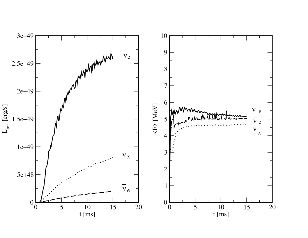
Figure 1: Testing for spurious neutrino emission: Shown are the luminosities of the various neutrino species (left) and the corresponding mean energies. After 15 ms, corresponding to $\sim$ 50 neutron star dynamical time scales, the total neutrino luminosity levels off four orders of magnitude below the emission of the full merger.

Neutron stars are expected to heat up during inspiral by tidal interaction to temperatures of the order $10^{8}$ K (Lai 1994). At these temperatures no significant neutrino emission will occur. In order to test for the amount of “spurious” emission of neutrinos in our simulation due to the unavoidable numerical heat up of the completely degenerate stars, we perform a test run (a listing of the different runs is provided in Table 1). We prepare a corotating equilibrium binary configuration just outside the last stable orbit by relaxing the two neutron stars in their mutual gravitational field. Subsequently we follow their dynamical evolution for approximately 50 neutron star dynamical time scales while they revolve on perfectly circular orbits around their common center of mass. Only self-gravity and hydrodynamic forces are considered, no initial radial velocities are applied and the gravitational wave backreaction forces are switched off. We find that the total neutrino luminosity reaches a stationary level of $\sim 3\cdot 10^{49}$ erg s^-1, see Fig. 1, which is four orders of magnitude below the peak luminosities of the full merger calculation and therefore completely negligible.

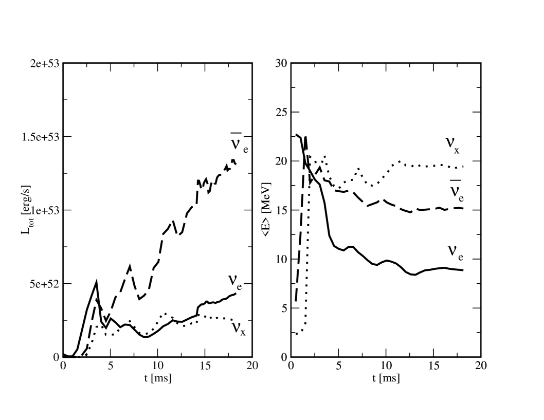
Figure 2: Run C (no spins, 2 x 1.4 ${\rm M_{\odot}}$): the left panel shows the luminosities (in ergs/s) of the different neutrino flavours. The right panel gives the corresponding mean energies. We regard this to be the generic case.

The overall neutrino emission properties of the full merger calculations are shown in Figs. 2 to 4. The total neutrino luminosities (left panels) are calculated summing up all particle contributions and the rms energies for each neutrino flavour are calculated according to eq. (20). For the corotating case, run D, substantial neutrino emission sets in later than in the cases without initial spin. The explanation for this is twofold: on the one hand this run starts out from numerically exact initial conditions while the non-rotating cases, run C and E, suffer an accelerated inspiral due to the start with initially spherical stars. On the other hand, neutrino emission only becomes important once the thick torus around the central high-density part has formed. Again this process takes longer for the corotating case since (due to the larger initial angular momentum) the torus-forming matter is initially launched into wider orbits. The average neutrino energies reach peak values soon after the stars have first come into contact. The reason for this is that the neutrinos from the hot debris material can, at this stage, escape without having to pass through any optically thick matter.
The total neutrino emission seems to have reached a roughly stationary level (except for maybe run C) by the end of the simulation. The total luminosities range from $\sim 10^{53}$ erg/s for the smoothly merging corotating case over $\sim 2\cdot 10^{53}$ erg/s for the irrotational case with twice 1.4 ${\rm M_{\odot}}$ to $\sim 4\cdot 10^{53}$ erg/s for our extreme case with 2 x 2.0 ${\rm M_{\odot}}$ and no initial spins. We regard run D as a lower limit which is unlikely to occur in nature (Bildsten & Cutler 1992, Kochanek 1992) and run C as the generic case since the observed neutron star binary systems have masses close to 1.4 ${\rm M_{\odot}}$ (Thorsett & Chakrabarti 1999) and are expected to have a very slow individual spin at the merger stage. The extreme case run E has been performed in order to explore the upper limit on the neutrino emission from the merger event.
The mean energies are $\sim$ 8 MeV for the electron-type neutrinos. This is below the typical values found in core collapse supernovae. The material in the nascent protoneutron star has first to deleptonize on a neutrino diffusion time scale before the electron fractions are as low as in the neutron star merger event, where beta-equilibrium has been established in the individual neutron stars long before the coalescence. Hence, the material in the supernova is more electron degenerate at comparable densities. Electrons are therefore captured from higher Fermi energies and produce electron neutrinos with a harder spectrum in the supernova case. The situation is different for the electron antineutrinos. We find rms energies around $\sim 15$ MeV, quite comparable to rms energies in the supernova case. The lower electron degeneracy in the neutron star merger favours the population of positrons, whose chemical potential has to balance the electron chemical potential because of pair equilibrium. The high positron abundance in combination with the neutron rich matter leads to more positron capture events on free neutrons than in the supernova. This results in higher electron anti-neutrino luminosities. The electron anti-neutrino luminosity from the remnant reaches up to $\sim 1.5\cdot 10^{53}$ erg/s, it provides the main cooling mechanism of the hot accretion disk. The heavy lepton neutrinos reach rms energies of $\sim 20$ to $\sim 25$ MeV. This is comparable to the supernova rms energies. Their luminosity, however, tends to be smaller in the neutron star merger case because the temperatures in the high density regimes, where the heavy lepton neutrinos emerge, are manifestly lower (see below).
To characterize the physical conditions of the emission region of each neutrino flavour we calculate average quantities, $\tilde{X}_{\nu_{i}}$, weighted by the $\nu_{i}$-number production rates per particle, $\tilde{R}^{ef}_{\nu_{i},j}$, where $X$ stands for $\rho,T,Y_{e}$ and $\mu_{e}$, given by

$$\tilde{X}_{\nu_{i}}=\frac{\sum_{j}\tilde{R}^{ef}_{\nu_{i},j}\;X_{j}}{\sum_{j}\tilde{R}^{ef}_{\nu_{i},j}}.$$ (9)

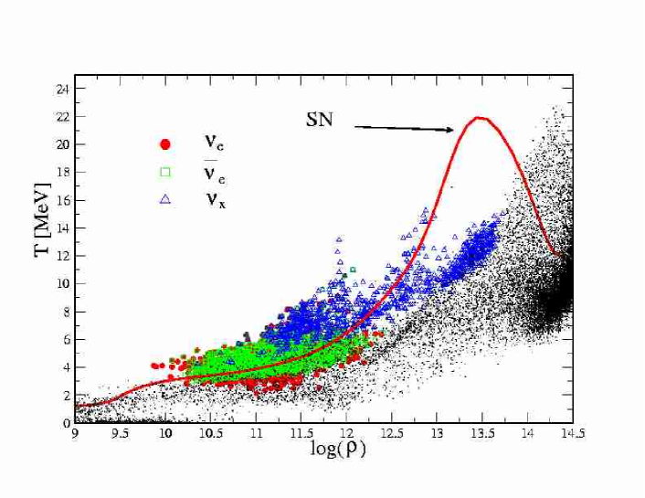
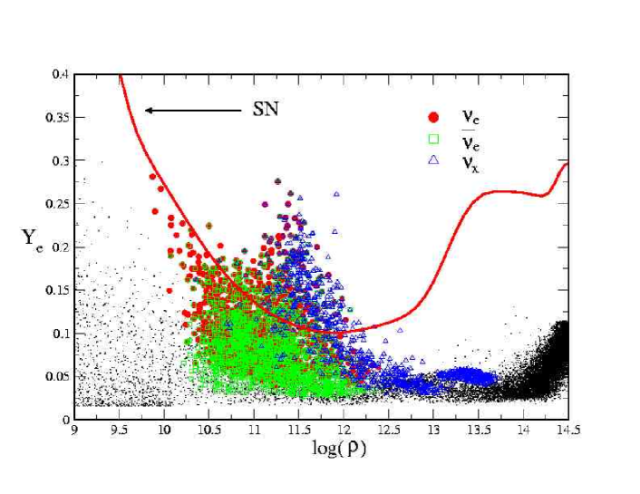
Figure 5: Shown are the SPH-particle distributions in the log($\rho)-T$- (upper panel) and the log($\rho)-Y_{e}$-plane (lower panel) of the generic case, run C (2 x 1.4 ${\rm M_{\odot}}$, no initial spin; every 20th particle is displayed as a dot). For comparison with the supernova (SN) case we show the conditions of a collapsed 13 ${\rm M_{\odot}}$ star, 100 ms after bounce as a thick line. The particles with the highest luminosities are also shown: filled circles for the $\nu_{e}$, squares for the $\bar{\nu}_{e}$ and the triangles refer to the $\nu_{x}$.

These quantities are displayed in Table 2. Electron neutrinos and anti-neutrinos are emitted under similar conditions, typically at densities around $10^{12.5}$ gcm^-3 , temperatures of 4-5 MeV (anti-neutrinos at slightly higher values) and a $Y_{e}$ below 0.1. The heavy lepton neutrinos are emitted at substantially higher densities (log$(\rho)\approx 13$) and temperatures ($T\approx$ 9 MeV).
Figure 5 shows a comparison between the conditions encountered in neutron star mergers and those of SNe. In the upper panel we show SPH-particle densities and temperatures (black dots, every 20th particle is shown) for our generic run C. Particles with peak luminosities are indicated with special symbols (these peak values are not to be confused with the average properties mentioned above). Filled circles indicate particles which emit $\nu_{e}$ at a luminosity in excess of 10 $\%$ of the maximum particle $\nu_{e}$-luminosity, squares mark the corresponding particles for $\bar{\nu}_{e}$ emission and triangles refer to $\nu_{x}$. Due to the steeper temperature dependence ($Q_{\nu_{x}}\propto T^{9}$) a lower threshold (3.5 $\%$) has been chosen for the $\nu_{x}$ in order to display roughly the same number of particles. The corresponding plot for $Y_{e}$ as a function of $\log(\rho)$ is shown in the second panel of Figure 5. We compare the state of these fluid elements to the state of fluid elements in a simulated postbounce evolution of the core of a $13$ M_⊙ progenitor star. Due to the limitation to spherical symmetry in this simulation with Boltzmann neutrino transport (Liebendörfer et al., 2002), the fluid elements form a solid line. In the supernova case, at $100$ ms after bounce, we find the peak emission at densities of $10^{10.6}$, $10^{11.3}$, and $10^{12.6}$ g/cm³ respectively. This is in agreement with the high emission regions identified in the neutron star merger for the heavy lepton neutrinos and the electron anti-neutrinos. The peak emission of electron neutrinos in the neutron star merger appears to occur at slightly higher densities ($\sim 10^{11}$ g/cm³). We attribute this to the less pronounced compression and deleptonization of infalling matter at low densities in the rotating accretion disk if compared to the failed explosion of a non-rotational supernova simulation. The heavy lepton neutrinos stem in both SN and neutron star merger from similar densities.
To analyze the importance of the e⁺/e^--capture reactions, eqs. (1) and (2), versus the pair producing reactions eqs. (3) and (4) we perform a post-processing experiment. We take one time-slice of our generic run, run C, at t= 14.1 ms and use the pair and plasma neutrino reactions as the only emission processes (i.e. the capture reactions are artificially switched off). In this case the luminosity in electron-type (anti-) neutrinos is only $\sim$ 10% of the previous values, indicating that a major contribution stems from the lepton capture reactions.

Table 2: Typical properties of emission region, densities are in gcm^-3, temperatures and chemical potentials in MeV.

run	$log(\tilde{\rho})_{\nu_{e}}$	$log(\tilde{\rho})_{\bar{\nu}_{e}}$	$log(\tilde{\rho})_{\nu_{x}}$	$\tilde{T}_{\nu_{e}}$	$\tilde{T}_{\bar{\nu}_{e}}$	$\tilde{T}_{\nu_{x}}$	$\tilde{Y}_{e,\nu_{e}}$	$\tilde{Y}_{e,\bar{\nu}_{e}}$	$\tilde{Y}_{e,\nu_{x}}$	$\tilde{\mu}_{e,\nu_{e}}$	$\tilde{\mu}_{e,\bar{\nu}_{e}}$	$\tilde{\mu}_{e,\nu_{x}}$
C	12.6	12.6	13.2	4.2	5.5	8.9	0.072	0.072	0.13	12.1	13.2	23.7
D	12.4	12.2	13.5	4.1	5.0	6.6	0.083	0.095	0.10	11.6	13.0	35.1
E	12.1	12.4	12.9	5.0	5.7	9.1	0.140	0.085	0.12	9.6	13.0	22.1

3.2 Emission geometry: disk versus central object

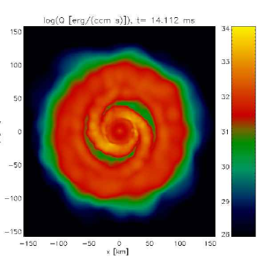
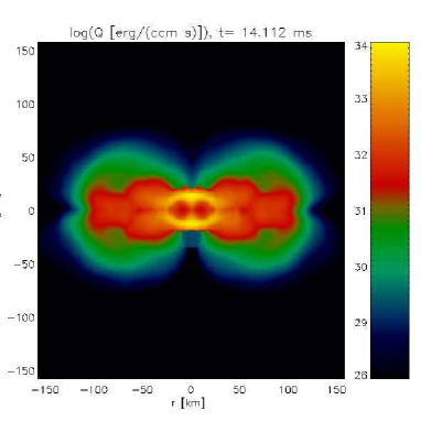
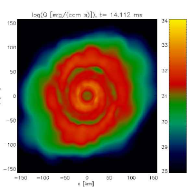
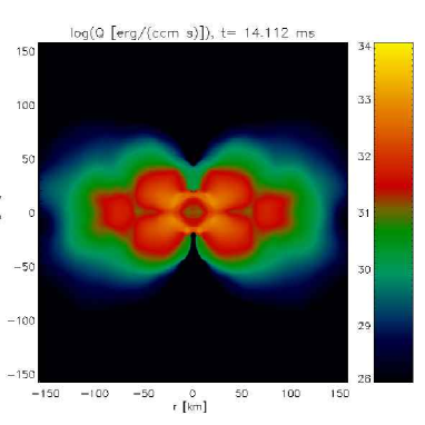
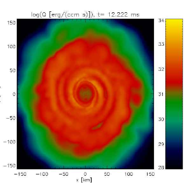
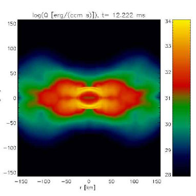
Figure 6: Geometry of the neutrino emission: the left column shows the total neutrino energy per time and volume in the orbital plane, the right column displays the vertical emission geometry. The upper two panels correspond to run C (2 x 1.4 ${\rm M_{\odot}}$, no spins), the middle panels to run D (2 x 1.4 ${\rm M_{\odot}}$, corotation) and the lowest panels to run E (2 x 2.0 ${\rm M_{\odot}}$, no spins). The contribution of the central object is negligible.

In Fig. 6 we plot the neutrino energy (sum of all flavours) per time and volume for run C (upper two panels), run D (intermediate two panels) and run E (the two lower panels). The left column of panels shows the emission in the orbital plane, while the vertical emission geometry (azimuthally averaged) is displayed in the right column. Note that the emission per time and volume from the hot, but extremely dense central objects is completely negligible, roughly two orders of magnitude lower than that coming from the most luminous parts of the disk. In paper I we had mentioned the butterfly-shaped temperature distribution in the XZ-plane that results from cool inflow being shock-heated hitting the inner parts of the disk, see Figure 15 in paper I. This pattern is also reflected in the neutrino emission geometry, see right column in Fig. 6.

3.3 Opacity sources: Importance of heavy nuclei

Our scheme accounts for the coherent scattering of neutrinos off heavy nuclei, for details we refer to the Appendix. We had realized that, despite the high temperatures encountered in the disk, matter finds it energetically favorable to form a non-negligible mass fraction of heavy nuclei (paper I). Due to the (approximate) proportionality of the scattering cross-section to the square of the nucleon number of the heavy nucleus, see (34), nuclei could possibly dominate as an opacity source. To estimate how important the heavy nuclei really are for the neutrino emission, we perform the following test. We take one time slice (t= 14.1 ms) of our generic case, run C, update the neutrino grid (see Appendix) and then calculate with these opacities the properties of the emitted neutrinos. In one case we use –like in the dynamical simulation– the full set of abundances given by the EOS for both the emission and absorption/scattering processes and in the other case we assume the matter to be completely dissociated into nucleons, i.e. the mass fractions are given by

$$x_{p}=Y_{e},\quad x_{n}=1-Y_{e},\quad x_{\alpha}=0,\quad x_{h}=0.$$ (10)

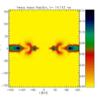
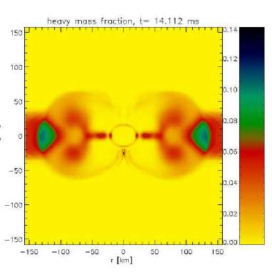
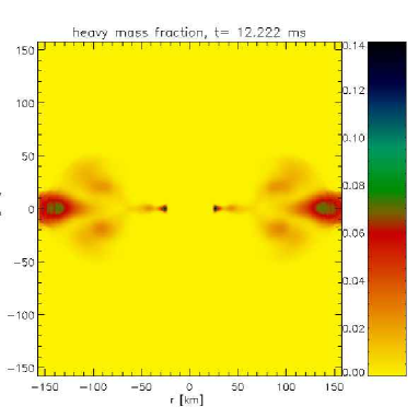
Figure 7: Shown are azimuthally averaged values of the heavy nucleus mass fraction for matter with $\rho>10^{10}$ g cm^-3 (top to bottom run C, D and E). Although heavy nuclei are present, neutrinos from the most luminous regions (see Fig. 6) can stream out vertically without encountering substantial amounts of heavy nuclei. Therefore the latter ones do not influence the total luminosity and the average energies.

We find almost exactly the same numbers for both the mean energies and the total luminosities, maximum deviations in the (more sensitive) total luminosities are below 5 %.
The reason for this lies in the geometry of the heavy nucleus distribution. In Fig. 7 we show the azimuthally averaged values of the heavy nucleus mass fraction, $x_{h}$, of runs C, D and E; these values are shown for matter with densities above 10¹⁰ gcm^-3, below that density matter is transparent to neutrinos. Nuclei are present in the cool, equatorial inflow regions identified in paper I, see Figure 15 in Rosswog and Davies (2002). The butterfly-shaped temperature distribution is also reflected in the nucleus mass fraction. It is interesting to note that despite the extreme temperatures in the central object a thin, nuclear crust can survive in our coolest case (run D). The hottest case (run E) is essentially free of heavy nuclei. By comparing Fig. 7 with Fig. 6, right column, it becomes obvious that the neutrinos from the most luminous regimes can escape in each case vertically without having to pass through material containing an interesting amount of heavy nuclei. Therefore the influence of the heavy nuclei onto the total luminosity and the mean energies is negligible.

3.4 Optical depths, neutrino-”spheres”

To illustrate how the opaque matter is distributed in the merger remnant we plot in Figures 8 to 10 contours of the spectrally averaged neutrino optical depth (see eq. (39) and (24)),

$$\tau_{\nu_{i}}=\chi_{\nu_{i}}\langle E^{2}_{\nu_{i}}\rangle=\chi_{\nu_{i}}\frac{F_{4}(\eta_{\nu_{i}})}{F_{2}(\eta_{\nu_{i}})}(kT)^{2}$$ (11)

for all neutrino species at the end of run C, D and E. The $F_{n}$ are the standard Fermi integrals, see Appendix A. Consistent with our neutrino treatment we have used the equilibrium values (see eq. (21)) for the degeneracy, $\eta$, of the $\nu_{e}$/$\bar{\nu}_{e}$ and have assumed a vanishing degeneracy parameter for the $\bar{\nu}_{x}$. In each of the Figures the uppermost panel shows contours of the optical depth of the electron neutrinos, the middle panels refer to the electron anti-neutrinos and the remaining ones to the heavy lepton neutrinos.

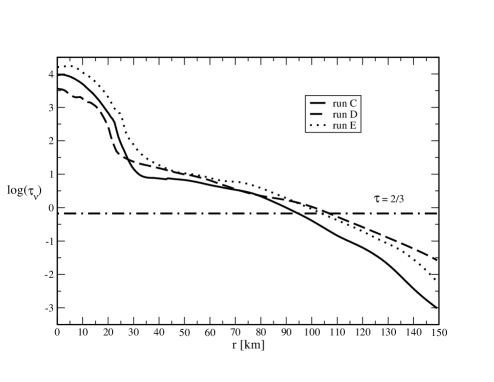
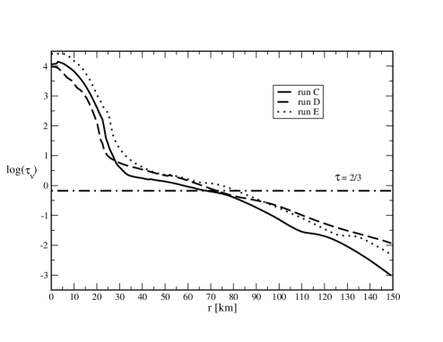
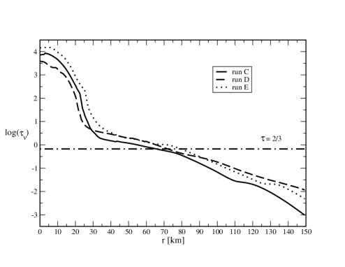
Figure 11: Optical depths at a height of z= 0 for the various neutrino flavours (top to bottom: $\nu_{e}$, $\bar{\nu}_{e}$, $\nu_{x}$).

The debris matter is most opaque to the electron-type neutrinos which in addition to scattering are also absorbed onto the copiously available free neutrons. Electron-type anti-neutrinos see matter less opaque and matter is most transparent to the $\nu_{x}$. We also show (as the thick line) the “neutrino-sphere”, defined as the locus with $\tau_{\nu_{i}}$= 2/3. For the $\bar{\nu}_{e}$ and the $\nu_{x}$ the neutrino-spheres almost coincide, with radial extensions of $\sim 70$ km and peak heights of $\sim 20$ km, since both neutrino types suffer essentially the same interactions (scattering events; in the extremely neutron-rich debris absorption onto free protons is only a minor correction). Due to their additional opacity sources the $\nu_{e}$ decouple substantially further out, at radial extensions of $\sim 105$ km with peak heights of $\sim 35$ km.
The optical depths at height z= 0, i.e. in the orbital plane, are shown in Figure 11 (from top to bottom: $\nu_{e}$, $\bar{\nu}_{e}$ and $\nu_{x}$). In the central object values up to several times $10^{4}$ are reached, beyond $\sim 130$ km matter is essentially transparent to neutrinos of all types, i.e. $\tau_{\nu_{i}}<0.1$.
It is interesting to note that it is only in the central object ($\tau_{\nu_{i}}>10$) that neutrinos are really trapped, see Figures 8 to 11. At the edge of the central object, at distances of $\sim 30$ km from the origin, the optical depth drops rapidly, but then only decreases very slowly throughout the disk ($\sim 30$ km to $\sim 100$ km). The whole hot torus-region is therefore in the semi-transparent regime.

3.5 Directional dependence of neutrino emission

It is consistent with our approach from eqs. (17) and (18) to think of the neutrinos emitted from an SPH-particle to be composed of “free neutrinos” and “diffusive neutrinos”. In analogy to general diffusion equations we assume that the diffusive neutrino component is emitted in the direction of the local, negative density gradient, $\hat{n}=-(\nabla{\rho})/|-(\nabla{\rho})|$. We use the SPH-prescription to determine this density gradient at the position of particle $i$:

$$\nabla{\rho}_{i}=\sum_{j}m_{j}\nabla_{i}W_{ij},$$ (12)

where $m_{j}$ is the particle mass, $W_{ij}=W(\frac{|\vec{x}_{i}-\vec{x}_{j}|}{h_{ij}})$ the standard SPH-kernel (e.g. Monaghan 1992) and $h_{ij}$ is the arithmetic mean of the involved smoothing lengths. The free component, in contrast, will emit isotropically. The fraction with which the both components contribute to the neutrino luminosity of particle $j$ is given by

$$f_{\nu_{i},Q_{j}}^{dif}=\frac{Q^{ef}_{\nu_{i},j}}{Q^{dif}_{\nu_{i},j}}\quad{\rm and}\quad f_{\nu_{i},Q_{j}}^{loc}=\frac{Q^{ef}_{\nu_{i},j}}{Q^{loc}_{\nu_{i},j}}.$$ (13)

It can be easily checked that $f_{\nu_{i},Q_{j}}^{dif}+f_{\nu_{i},Q_{j}}^{loc}=1$ by using eqs. (17) and (18) and that the fractions approach their obvious limits in the high and low-density regimes. Similarly, fractions of the emitted neutrino number, $f_{\nu_{i},R_{j}}^{dif}$ and $f_{\nu_{i},R_{j}}^{loc}$ can be defined as above, but with number emission rates per volume, $R_{\nu_{i},j}$, rather than with energy emission rates per volume, $Q_{\nu_{i},j}$. With these definitions the neutrino luminosity per solid angle, composed of a diffusive and a free component, is determined by

$$\Lambda_{\nu_{i}}(\vartheta)=\frac{\Delta L_{\nu_{i}}}{\Delta\Omega}=\frac{\sum_{k}\tilde{Q}_{\nu_{i},k}^{dif}(\vartheta)}{2\pi\sin(\vartheta)\Delta\vartheta}+\frac{\sum_{j}\tilde{Q}_{\nu_{i},j}^{loc}}{4\pi}.$$ (14)

Here $\tilde{Q}_{\nu_{i},k}$ is the $\nu_{i}$ energy emission rate of particle $k$, from either “diffusive” neutrinos, $\tilde{Q}^{dif}_{\nu_{i},k}=f_{\nu_{i},Q_{k}}^{dif}\cdot\tilde{Q}^{ef}_{\nu_{i},k}$ or “free” neutrinos, $\tilde{Q}^{loc}_{\nu_{i},k}=f_{\nu_{i},Q_{k}}^{loc}\cdot\tilde{Q}^{ef}_{\nu_{i},k}$. In the above equation the $j$-sum extends over all the particles (since their “free” neutrinos radiate isotropically), the $k$-sum, however, only extends over those particles that radiate into a ring of width $\Delta\vartheta$ in the $\vartheta$-direction, $\vartheta-\Delta\vartheta/2<\vartheta_{k}<\vartheta+\Delta\vartheta/2$, where $\vartheta_{k}$ is given by $\cos(\vartheta_{k})=\hat{n}_{k}\cdot\hat{e}_{z}$. An observer that sees the merger from an angle $\vartheta$ with respect to the initial binary rotation axis (= z-axis) would thus infer an apparent luminosity of

$$L_{\nu_{i}}^{\rm app}(\vartheta)=4\pi\Lambda_{\nu_{i}}(\vartheta).$$ (15)

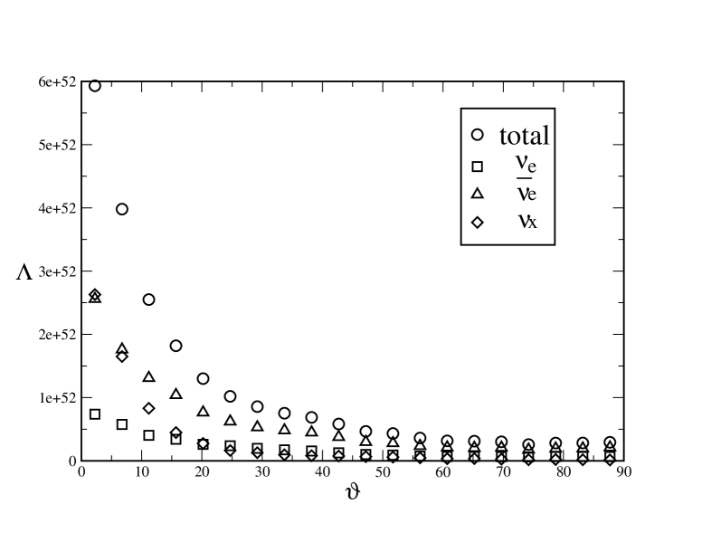
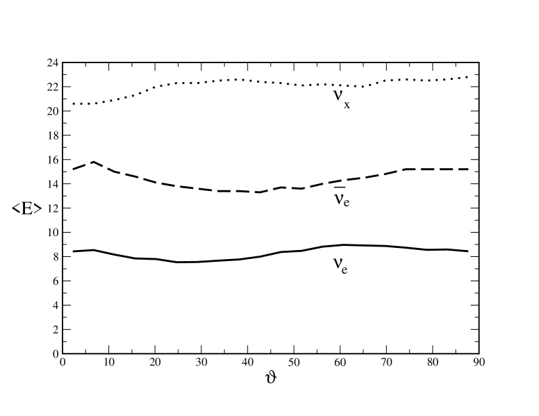
Figure 12: Directional dependence of the neutrino emission: the upper panel shows the neutrino luminosity per solid angle, $\Lambda_{\nu_{i}}(\vartheta)=\frac{\Delta L_{\nu_{i}}}{\Delta\Omega}$ as a function of the angle (with the original binary rotation axis) under which the system is observed. The apparent luminosity is given by $L^{\rm app}_{\nu_{i}}=4\pi\Lambda_{\nu_{i}}$. The lower panel shows the rms average energies of the neutrinos as a function of $\vartheta$.

The quantity $\Lambda_{\nu_{i}}(\vartheta)$ for our generic case, run C, is shown in Fig. 12 (the other runs yield similar results). The luminosity per solid angle is peaked towards the z-axis: a system observed “pole-on” ($\vartheta\approx 0^{\circ}$) will yield a total neutrino energy flux, given by $f_{\nu_{i}}(\vartheta)=\frac{\Lambda_{\nu_{i}}(\vartheta)}{R^{2}}$, $R$ being the distance to the source, that is around 20 times larger than that of a system that is observed “edge-on” ($\vartheta\approx 90^{\circ}$). This preferential emission is visible for all neutrino flavours, but most pronounced in the case of the heavy lepton neutrinos, $\nu_{x}$. The latter ones are produced in the enormously temperature dependent reactions (3) and (4) and therefore emerge from the hottest parts of the remnant, i.e. they are generated within or close to the flattened central object, where the density gradients point along the z-direction.

To infer the $\vartheta$-dependence of the average neutrino energies we use the quantitity

$$\epsilon_{\nu_{i}}(\vartheta)=\sqrt{\frac{\sum_{j}\tilde{R}^{ef}_{\nu_{i},j}E^{2}_{\nu_{i},j}(f_{\nu_{i},R_{j}}^{dif}\cdot\Theta_{j}(\vartheta)+f_{\nu_{i},R_{j}}^{loc})}{\sum_{j}\tilde{R}^{ef}_{\nu_{i},j}(f_{\nu_{i},R_{j}}^{dif}\cdot\Theta_{j}(\vartheta)+f_{\nu_{i},R_{j}}^{loc})}}.$$ (16)

Here, the $j$-sum extends over all the particles; to count only the contributing particles in the diffusive part, the function

$$\Theta_{j}(\vartheta)=\left\{\begin{array}[]{r@{ }l}&2/(\sin(\vartheta)\Delta\vartheta)\quad\mbox{for }\quad\vartheta-\Delta\vartheta/2<\vartheta_{j}<\vartheta+\Delta\vartheta/2\\ &0\;\quad\quad\quad\quad\quad\quad\mbox{else}\end{array}\right.$$

has been introduced. The distribution of the average energies, see second panel Fig. 12, is relatively flat for all neutrino types.

4 Summary and Discussion

We have presented the neutrino emission results from our high-resolution simulations of the coalescence of two neutron stars. We find typically total neutrino luminosities of $\sim 2\cdot 10^{53}$ erg/s with rms energies of $\sim 8$ MeV for electron type neutrinos, $\sim 15$ MeV for their anti-particles and $\sim 20-25$ MeV for the $\mu$- and $\tau$-neutrinos and their antiparticles. We have performed two runs that are intended to give an upper and a lower limit to the total neutrino luminosities: in the case of initial corotation the stars merge extremely smoothly. This goes along with moderately high matter temperatures and neutrino luminosities lower by a factor of two than in our standard case. In the other extreme case we consider the coalescence of two 2.0 ${\rm M_{\odot}}$ neutron stars without initial spins. This case leads to the hottest merger remnant and, correspondingly, to the highest neutrino luminosities, around $4\cdot 10^{53}$ erg/s.
The contributions of the extremely hot, but also neutrino-opaque central objects are marginal, typically only a few percent. Most neutrinos are produced in the debris torus around the central object, which exhibits temperatures well above the positron production threshold and which is very neutron rich ($Y_{e}\sim 0.1$). These conditions favour positron captures on free neutrons over electron captures and therefore yield neutrino luminosities which are clearly dominated by the $\bar{\nu}_{e}$. The heavy lepton neutrinos contribute only $\sim 10\%$ to the total luminosity. The $\nu_{e}$ and $\bar{\nu}_{e}$ are predominantly produced in electron and positron captures on free nucleons, only $\sim 10\%$ come from the pair and plasma process. The whole disk, with distances of $\sim 30$ km to $\sim$ 100 km is semi-tranparent to the neutrinos; it is only within the high-density central object that they are really trapped ($\tau_{\nu_{i}}>10$).
We find qualitative agreement with the results described in Ruffert and Janka (2001) as far as the dominance of the $\bar{\nu}_{e}$ and the hierarchies in the rms neutrino energies ($\epsilon_{\nu_{e}}<\epsilon_{\bar{\nu}_{e}}<\epsilon_{\nu_{x}}$) are concerned. Our total luminosities and rms energies, however, are lower than those found in their models, typically by a factor of $\sim 2$ in the luminosities and around $\sim 20\%$ in the mean energies. This comes in part from the fact that not exactly the same initial conditions are used: the ’standard’ mass they use is 1.6 ${\rm M_{\odot}}$ rather than our value, 1.4 ${\rm M_{\odot}}$. This mass difference is expected to lead to slightly increased luminosities. Another difference is the EOS. The EOS of Shen et al. (1998) that we use is in the density regime of 12 $<$ log($\rho$) $<$ 14, where large fractions of the neutrino emission stems from, substantially stiffer than the Lattimer-Swesty EOS that Ruffert & Janka use (compare Fig. 2 in Rosswog & Davies 2002). This leads to a less compact configuration with lower temperatures and correspondingly lower neutrino luminosities in our case. Further possibilities include a different amount of numerical viscosity (see Rosswog & Davies 2002 for a discussion) in both codes and maybe the interaction with the background medium in the simulations of Ruffert & Janka (2001; see their paper for a discussion of this point). Finally, the lower luminosities may also come from differences in the leakage prescriptions. However, as shown in the appendix, if at all, our scheme tends to overestimate the luminosities. Therefore the true neutrino luminosities could be even lower, a fact that has serious consequences for the ability of neutron star mergers to produce a gamma-ray burst fireball via neutrino annihilation. This is discussed further in Rosswog & Ramirez-Ruiz (2002) and Rosswog et al. (2003).
Despite the high temperatures we find areas in the disk that contain a substantial mass fraction of heavy nuclei. One might expect this to influence the neutrino luminosities, since the coherent scattering cross sections are $\propto A^{2}$, where $A$ is the nucleon number of the nucleus. This, however, is not the case. In each of the investigated cases the most neutrino-luminous parts of the remnant are essentially free of heavy nuclei and the neutrinos can always escape via almost completely photo-dissociated matter.
We find that the neutrino emission per solid angle is focussed towards the initial binary rotation axis. A merger remnant observed “pole-on” has an apparent neutrino luminosity that is about 20 times larger than a remnant seen “edge-on”.
A typical neutron star merger produces mean neutrino energies very similar to those resulting from the core collapse of a massive star. A distinctive signature between both events is the strong dominance of the electron anti-neutrinos over electron neutrinos in the merger case. The most unique proof, however, for neutrinos coming from a neutron star coalescence rather than from a SN would be the nearly coincident detection of a binary “chirp”-signal in gravitational waves. The peak luminosity in neutrinos will be reached about 15 ms after the peak in the gravitational wave luminosity.

Acknowledgements

It is a pleasure to thank E. Ramirez-Ruiz, R. Speith and the Leicester theory group for fruitful discussions. This work has benefited from the excellent support from the Leicester supercomputer team Stuart Poulton, Chris Rudge and Richard West. Most of the computations reported here were performed using the UK Astrophysical Fluids Facility (UKAFF). Part of this work has been performed using the University of Leicester Mathematical Modelling Centre’s supercomputer which was purchased through the EPSRC strategic equipment initiative. This work was supported by a PPARC Rolling Grant for Theoretical Astrophysics. S.R. gratefully acknowledges the support of PPARC by an Advanced Fellowship. M. L. acknowledges support by the NSF under contract AST-9877130 at the University of Tennessee, Knoxville and the Oak Ridge National Laboratory, managed by UT-Batelle, LLC, for the U.S. Department of Energy under contract DE-AC05-00OR22725.

Appendix A Neutrino treatment

The rates that we use in the simulations are smooth interpolations between diffusion and local production rates. If we denote for a given neutrino species $\nu_{i}$ the number emission rates by $R_{\nu_{i}}$ per volume and energy emission rates per volume by $Q_{\nu_{i}}$, our prescription for the effective rates reads

$$R_{\nu_{i}}^{ef}=R_{\nu_{i}}^{loc}\left(1+\frac{R_{\nu_{i}}^{loc}}{R_{\nu_{i}}^{dif}}\right)^{-1}$$ (17)

$$Q_{\nu_{i}}^{ef}=Q_{\nu_{i}}^{loc}\left(1+\frac{Q_{\nu_{i}}^{loc}}{Q_{\nu_{i}}^{dif}}\right)^{-1}.$$ (18)

This ansatz is similar to the one used in Ruffert et al. (1996). Here the quantities with the superscript “$loc$” denote the locally produced rates of number and energy while the superscript “$dif$” refers to the diffusion rates that are further specified below. In the transparent regime, where the diffusion time scale $T^{dif}_{\nu_{i}}$ is short, and therefore $R_{\nu_{i}}^{dif}\gg R_{\nu_{i}}^{loc}$ and $Q_{\nu_{i}}^{dif}\gg Q_{\nu_{i}}^{loc}$ all the locally produced neutrinos stream out freely. In the very opaque regime, where $T^{dif}_{\nu_{i}}$ is large, the neutrinos leak out on the diffusion time scale. Therefore both limits are treated correctly, the regime inbetween these limits is handled via interpolation.
The mean neutrino energy of each SPH-particle (particle index suppressed) is then found from

$$E^{ef}_{\nu_{i}}=\frac{\sum_{r}Q^{ef}_{\nu_{i},r}}{\sum_{r}R^{ef}_{\nu_{i},r}},$$ (19)

where $r$ labels all reactions producing neutrinos of type ${\nu_{i}}$. Note, that these (mean) energies are used exclusively for book-keeping purposes, in all places where a dependence on neutrino energies occurs, we integrate cross-sections over a Fermi-distribution (see below).
To characterize the average neutrino energies of the total system we use rms energies given by

$$\epsilon_{\nu_{i}}=\sqrt{\frac{\sum_{j}\tilde{R}^{ef}_{\nu_{i},j}(E^{ef}_{\nu_{i},j})^{2}}{\sum_{j}\tilde{R}^{ef}_{\nu_{i},j}}},$$ (20)

where $j$ labels the SPH-particles and $\tilde{R}^{ef}_{\nu_{i},j}$ is the rate of neutrino number emission of particle $j$ (not to be confused with the rate per volume, $R^{ef}_{\nu_{i},j}$).
We have tested this scheme in spherical symmetry against stationary state Boltzmann transport (Mezzacappa & Messer 1999). To this end we determined the neutrino properties for a frozen matter background. The background properties ($\rho,T$ and $Y_{e}$) were either taken from neutron star merger (Rosswog & Davies 2002) or core collapse supernova simulations (Liebendörfer et al. 2002). While the rms neutrino energies agree within 20 $\%$ the accuracy of the luminosities depends on the importance of the semi-transparent regime where the interpolation (eqs. (17) and (18)) is applied. In the worst case we found that our scheme overestimates the luminosities by a factor 3-4.

A.1 Free Emission Rates

In the following we will neglect the electron mass and the nucleon mass difference, $Q=m_{n}-m_{p}=1.2935$ MeV, in all the cross sections (Tubbs & Schramm 1975). This is appropriate for our purposes and largely simplifies the involved rate expressions. We further assume the neutrino temperature to be identical to the local matter temperature and, where necessary, we assume the neutrinos to follow a Fermi-distribution. The chemical potentials of the $\nu_{x}$ are generally assumed to vanish, for $\nu_{e}$ and $\bar{\nu}_{e}$ we apply the equilibrium values

$$\mu_{\nu_{e}}=-\mu_{\bar{\nu}_{e}}=\bar{\mu}_{e}-\hat{\mu}-Q,$$ (21)

wherever they occur in the sequel. Here $\bar{\mu}_{e}$ is the electron chemical potential (with rest mass) and $\hat{\mu}$ is the difference in the neutron and proton chemical potentials (without rest mass). Degeneracy parameters $\mu_{i}/T$ are denoted by $\eta_{i}$, temperatures are always in units of energies.
With these approximations and ignoring momentum transfer to the nucleon (Bruenn 1985) the electron capture rate per volume reads

$$R_{EC}=\beta\;\eta_{pn}T^{5}F_{4}(\eta_{e}),,$$ (22)

with

$$\beta=\frac{\pi}{h^{3}c^{2}}\frac{1+3\alpha^{2}}{(m_{e}c^{2})^{2}}\sigma_{0}.$$ (23)

Here $h$ is Planck’s constant and $c$ the speed of light, $\alpha\approx 1.25$, $m_{e}$ is the electron mass, $\sigma_{0}\approx 1.76\cdot 10^{-44}$cm². $F_{n}$ is a Fermi integral given by

$$F_{n}(z)=\int_{0}^{\infty}\frac{x^{n}dx}{e^{x-z}+1}$$ (24)

and can be efficiently evaluated via series expansions (Takahashi et al. 1978). The factor $\eta_{pn}$ given by

$$\eta_{pn}=\frac{n_{n}-n_{p}}{exp(\hat{\mu}/T)-1},$$ (25)

takes into account the nucleon final state blocking and reduces in the non-degenerate limit to the proton number density $n_{p}$, $n_{n}$ refers to the neutron number density. Following the analogous procedure one finds for the energy emission rate

$$Q_{EC}=\beta\,\eta_{pn}T^{6}F_{5}(\eta_{e}),$$ (26)

and for the mean energy of the emitted neutrinos

$$\langle E_{\nu_{e}}\rangle_{EC}=\frac{Q_{EC}}{R_{EC}}=T\frac{F_{5}(\eta_{e})}{F_{4}(\eta_{e})}.$$ (27)

The corresponding rates for positron captures read

$$R_{PC}=\beta\,\eta_{np}T^{5}F_{4}(-\eta_{e}),$$ (28)

$$Q_{PC}=\beta\,\eta_{np}T^{6}F_{5}(-\eta_{e}),$$ (29)

$$\langle E_{\bar{\nu}_{e}}\rangle_{PC}=T\frac{F_{5}(-\eta_{e})}{F_{4}(-\eta_{e})},$$ (30)

where $\eta_{np}$ is obtained from $\eta_{pn}$ by interchanging the neutron and proton properties.
The “thermal” processes are taken into account via fit formulae. For the energy emission from the pair process we use the prescription of Itoh et al. (1996). The number emission rate is obtained by deviding by the mean energy per neutrino pair (Cooperstein et al. 1986)

$$\langle E_{\nu_{i}\bar{\nu}_{i}}\rangle_{pair}=T\left(\frac{F_{4}(\eta_{e})}{F_{3}(\eta_{e})}+\frac{F_{4}(-\eta_{e})}{F_{3}(-\eta_{e})}\right).$$ (31)

For the plasmon decay we use the formulae of Haft et al. (1994) with

$$\langle E_{\nu_{i}\bar{\nu}_{i}}\rangle_{\gamma}=T\left(2+\frac{\gamma^{2}}{1+\gamma}\right),$$ (32)

where $\gamma=\gamma_{0}\sqrt{\pi^{2}/3+\eta_{e}^{2}}$ and $\gamma_{0}=5.565\cdot 10^{-2}$.

A.2 Diffusive Emission Rates

In order to evaluate the opacities along given directions we map the particle properties density, temperature and electron fraction on an aequidistant, cylindrical grid with coordinates $(R,Z)$, where $R=\sqrt{x^{2}+y^{2}}$, see Figure 13. The assumption of rotational symmetry around the binary rotation axis is an excellent approximation since the main neutrino emitting region is the hot, neutron star matter debris torus that forms around the merged central object (see Fig. 14 in paper I). By evaluating the EOS at each grid point the matter properties (like the local composition) are known and we can therefore assign a variable $\zeta_{\nu_{i}}$ (see eq. (37)), containing compositional information, to each grid point. The neutrino grid does not have to be updated at every hydro time step. We chose to update it after a small fraction (1/8) of the neutron star dynamical time scale, $\tau_{dyn}=(G\bar{\rho})^{-1/2}\approx 2\cdot 10^{-4}$ s, which is a tiny fraction of the timescale on which typical disk properties change. Once all the properties on the grid are known, the desired values at the SPH-particle positions are found by trilinear interpolation. We use 400 points in radial direction and 300 points in positive Z-direction (symmetry with respect to the orbital plane is an excellent approximation for the systems under investigation).

The dominant sources of opacity are

• neutrino nucleon scattering:

  $$\nu_{i}+\{n,p\}\rightarrow\nu_{i}+\{n,p\}$$ (33)

  with $\sigma_{\nu_{i},nuc}=\frac{1}{4}\sigma_{0}\left(\frac{E_{\nu_{i}}}{m_{e}c^{2}}\right)^{2}$ (Shapiro & Teukolsky 1983) and

• coherent neutrino nucleus scattering:

  $$\nu_{i}+A\rightarrow\nu_{i}+A$$ (34)

  with $\sigma_{\nu_{i},A}=\frac{1}{16}\sigma_{0}\left(\frac{E_{\nu_{i}}}{m_{e}c^{2}}\right)^{2}A^{2}(1-Z/A)^{2}$ (Shapiro & Teukolsky 1983; $\sin^{2}\theta_{W}$ has been approximated by 0.25). Here $A$ and $Z$ are the nucleon and proton number of the average nucleus whose properties are stored in our EOS-table. Due to the $A^{2}$-dependence of the cross section this process will dominate as soon as a substantial fraction of heavy nuclei is present (remember that the nucleon numbers in these nuclei reach values of up to $\sim$ 400 Shen et al. 1998).
  Electron type neutrinos additionally undergo

• neutrino absorption:

  $$\nu_{e}+n\rightarrow p+e^{-}$$ (35)

  $$\bar{\nu}_{e}+p\rightarrow n+e^{+}$$ (36)

  with $\sigma_{\nu_{e},n}=\frac{1+3\alpha^{2}}{4}\sigma_{0}\left(\frac{E_{\nu}}{m_{e}c^{2}}\right)^{2}\langle 1-f_{e^{-}}\rangle$, where $\langle 1-f_{e^{-}}\rangle\approx\left({\rm exp}(\eta_{e}-F_{5}(\eta_{\nu_{e}})/F_{4}(\eta_{\nu_{e}}))+1\right)^{-1}$
  and $\sigma_{\bar{\nu}_{e},p}=\frac{1+3\alpha^{2}}{4}\sigma_{0}\left(\frac{E_{\bar{\nu}}}{m_{e}c^{2}}\right)^{2}\langle 1-f_{e^{+}}\rangle$, $\langle 1-f_{e^{+}}\rangle\approx\left({\rm exp}(-\eta_{e}-F_{5}(\eta_{\bar{\nu}_{e}})/F_{4}(\eta_{\bar{\nu}_{e}}))+1)\right)^{-1}$.

The local mean free path is given by (where for simplicity the spatial dependence is suppressed)

$$\lambda_{\nu_{i}}(E)=\left(\sum_{r}n_{r}\sigma_{r}(E)\right)^{-1}\equiv(E^{2}\zeta_{\nu_{i}})^{-1},$$ (37)

where the $n_{r}$ denote the target number densities, the index $r$ runs over the reactions given above with cross-sections $\sigma_{r}$ and $E$ is the neutrino energy. The dependence of the cross-sections on the squared neutrino energies has been separated out in the definition of $\zeta_{\nu_{i}}$. The optical depth, $\tau$, along a specified direction is then given as

$$\tau_{\nu_{i}}(E)=\int_{x1}^{x2}\frac{dx}{\lambda_{\nu_{i}}(E)}.$$ (38)

The optical depths are evaluated along three directions from each grid point: in Z-direction ($\tau^{1}_{\nu_{i}}$), i.e. parallel to the rotational axis, along the outgoing diagonal ($\tau^{2}_{\nu_{i}}$) and along the ingoing diagonal ($\tau^{3}_{\nu_{i}}$), see Fig. 13. The finally used optical depth, ($\tau_{\nu_{i}}$), is the minimum of the three, $\tau_{\nu_{i}}={\rm min}(\tau^{1}_{\nu_{i}},\tau^{2}_{\nu_{i}},\tau^{3}_{\nu_{i}}$). The quantities that are actually stored for each grid point $j$ are

$$\chi^{d}_{j,\nu_{i}}=\int_{d,j}\zeta_{\nu_{i}}(x)dx,$$ (39)

where $d$ denotes the direction and $\int_{d,j}dx$ is the integration from grid point j along direction $d$. Note that the quantity $\chi$ is independent of the neutrino energy and the (energy dependent) optical depth is given by

$$\tau_{\nu_{i}}(E)=E^{2}{\rm min}_{d}(\chi_{j,\nu_{i}}^{d})\equiv E^{2}\chi_{j,\nu_{i}}.$$ (40)

The diffusion rate depends on the optical depth $\tau_{\nu_{i}}$. We base our estimates on a very simple, one-dimensional diffusion model. Along one propagation direction we assume equal probabilities for forward and backward scattering and impose strict flux conservation in a stationary state situation. This leads to the following relationship between the neutrino density $J(E)$ and the neutrino number flux $H(E)$,

$$\frac{H_{\nu_{i}}(E)}{cJ_{\nu_{i}}(E)}=\frac{1}{2\tau_{\nu_{i}}(E)+1}.$$ (41)

We can test this relationship against a complete numerical solution of the diffusion equation in e.g. a supernova environment where all relevant opacities are included and find agreement to about a factor of two. If the thermodynamical conditions and the neutrino densities along the propagation direction are set, relation (41) defines a local neutrino number flux $H_{\nu_{i}}(E)$ which in general no longer obeys flux conservation in a stationary state situation. Assuming that we still have a stationary state situation and that the fluxes are locally well represented, we can use the balance of fluxes across a infinitesimally thin layer perpendicular to the propagation direction to obtain an estimate of the rate $R_{\nu_{i}}$ of neutrinos produced in this layer. Denoting the propagation direction with $x$, we express the rate in terms of the prevailing neutrino density and a diffusion time scale $T_{\nu_{i},x}^{dif}$ with

$$R_{\nu_{i}}^{dif}(E)=\frac{\partial H_{\nu_{i}}(E)}{\partial x}=\frac{J_{\nu_{i}}(E)}{T_{\nu_{i}}^{dif}(E)}.$$ (42)

The substitution of eq. (41) for $H_{\nu_{i}}$ leads to spatial derivatives of the neutrino density $J_{\nu_{i}}(E)$ and the optical depth $\tau_{\nu_{i}}$. As the latter is given by the negative inverse mean free path, $-1/\lambda_{\nu_{i}}(E)$, eq. (42) can be resolved for the diffusion time scale according to

$$T_{\nu_{i}}^{dif}(E)=\frac{2\tau_{\nu_{i}}(E)+1}{c}\left(\frac{\partial\ln J_{\nu_{i}}(E)}{\partial x}+\frac{2}{\left(2\tau_{\nu_{i}}(E)+1\right)\lambda_{\nu_{i}}(E)}\right)^{-1}.$$ (43)

We rewrite this estimate with a distance parameter, $\Delta x(E)$, to obtain

$$T_{\nu_{i}}^{dif}(E) = \frac{\Delta x_{\nu_{i}}(E)}{c}\left(2\tau_{\nu_{i}}(E)+1\right),$$ (44)

$$\Delta x_{\nu_{i}}(E) = \left(\frac{\partial\ln J_{\nu_{i}}(E)}{\partial x}+\frac{2}{\left(2\tau_{\nu_{i}}(E)+1\right)\lambda_{\nu_{i}}(E)}\right)^{-1}.$$ (45)

The spatial derivative of the neutrino density in eq. (45) is quite inconvenient, one would prefer a diffusion time scale that does not depend on neutrino densities. Moreover, the derivative is likely to introduce noise when evaluated in a three-dimensional numerical simulation. Hence, we neglect this term. In physical terms this means that we assume neutrino sources that keep the neutrino density close to constant over a spatial interval where the mean free path changes significantly. This might not always be justified and is subject to future improvement. The expression for the distance parameter, however, greatly simplifies to

$$\Delta x_{\nu_{i}}(E)=\left(\tau_{\nu_{i}}(E)+\frac{1}{2}\right)\lambda_{\nu_{i}}.$$ (46)

Here we recall that Ruffert et al. (1996) found the dependence

$$T_{\nu_{i}}^{dif}(E)=3\frac{\Delta x_{\nu_{i}}(E)}{c}\tau_{\nu_{i}}(E)$$ (47)

by calibration with a numerical neutrino transport scheme. If we go back and use $\tau_{\nu_{i}}\sim 1$ for the “last interaction region” to simplify eq. (41) further by the approximation

$$\frac{H_{\nu_{i}}(E)}{cJ_{\nu_{i}}(E)}=\frac{1}{3\tau_{\nu_{i}}(E)},$$

we obtain eq. (47) by the same analysis used to derive eq. (44). However, the distance parameter is then given by

$$\Delta x_{\nu_{i}}(E)=\tau_{\nu_{i}}(E)\lambda_{\nu_{i}}(E).$$ (48)

In our scheme $\Delta x$ defines the effective width of a layer drained by the diffusive flux, i.e. provides the conversion between a net emitted neutrino flux (number/s/cm^2) and a production rate (number/s/cm^3). We choose eqs. (47) and (48) for our numerical simulations because the linear dependence in $\tau_{\nu_{i}}$ allows the extraction of the energy dependence as in eq. (40). Approximating the neutrino distribution function in the high-density regime with a thermal equilibrium distribution we apply the diffusion time scale and obtain the diffusion rates

$$\langle R^{dif}_{\nu_{i}}\rangle=\int_{0}^{\infty}\frac{\tilde{n}_{\nu_{i}}(E)}{T^{dif}_{\nu_{i}}(E)}dE=\frac{4\pi cg_{\nu_{i}}}{(hc)^{3}}\frac{\zeta_{\nu_{i}}}{3\chi^{2}_{\nu_{i}}}TF_{0}(\eta_{\nu_{i}})$$ (49)

$$\langle Q^{dif}_{\nu_{i}}\rangle=\int_{0}^{\infty}\frac{E\tilde{n}_{\nu_{i}}(E)}{T^{dif}_{\nu_{i}}(E)}dE=\frac{4\pi cg_{\nu_{i}}}{(hc)^{3}}\frac{\zeta_{\nu_{i}}}{3\chi^{2}_{\nu_{i}}}T^{2}F_{1}(\eta_{\nu_{i}})$$ (50)

with

$$\langle E^{dif}_{\nu_{i}}\rangle=\frac{\langle Q^{dif}_{\nu_{i}}\rangle}{\langle R^{dif}_{\nu_{i}}\rangle}=T\frac{F_{1}(\eta_{\nu_{i}})}{F_{0}(\eta_{\nu_{i}})}.$$ (51)

Here $\tilde{n}_{\nu_{i}}(E)$ is related to the number density by $n_{\nu_{i}}=\int_{0}^{\infty}\tilde{n}_{\nu_{i}}(E)dE$. The statistical weights $g_{\nu_{i}}$ are 1 for $\nu_{e}$ and $\bar{\nu}_{e}$ and 4 for $\nu_{x}$. After the second equals sign in eqs. (49) and (50) we have inserted the explicit estimate (47) for the diffusion time scale and (48) for the distance parameter. Note that this leakage prescription is not based on the use of mean neutrino energies, eq. (19) is exclusively used for informative purposes. Our scheme accounts for the energy dependence of the neutrino opacities by integrating over the neutrino distribution.

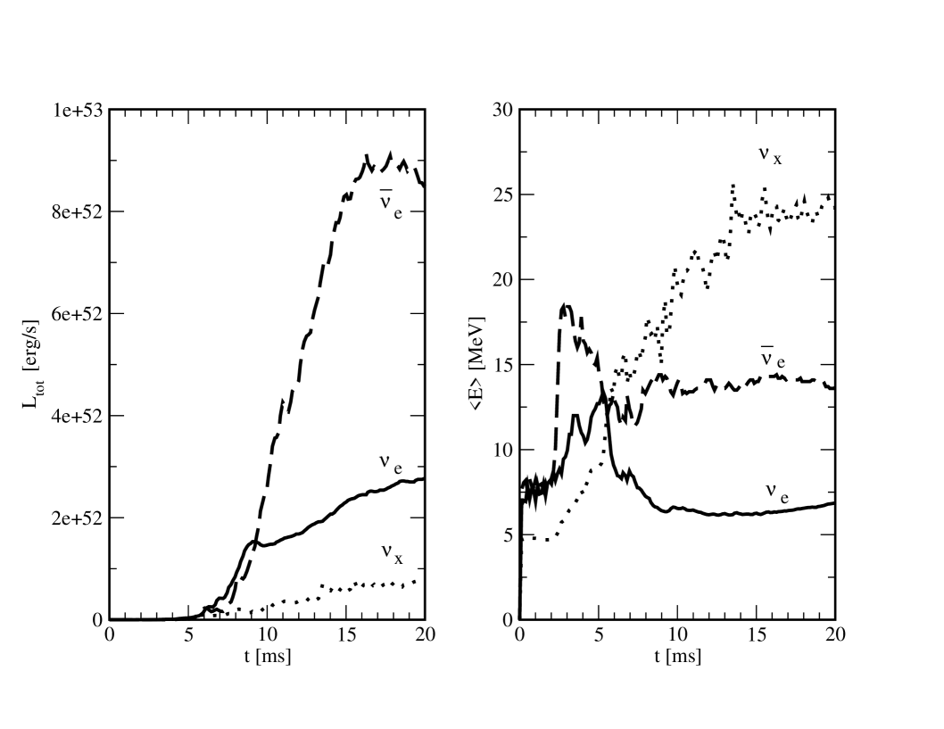
Figure 3: Run D (corotation, 2 x 1.4 ${\rm M_{\odot}}$): the left panel shows the luminosities (in ergs/s) of the different neutrino flavours. The right panel gives the corresponding mean energies.

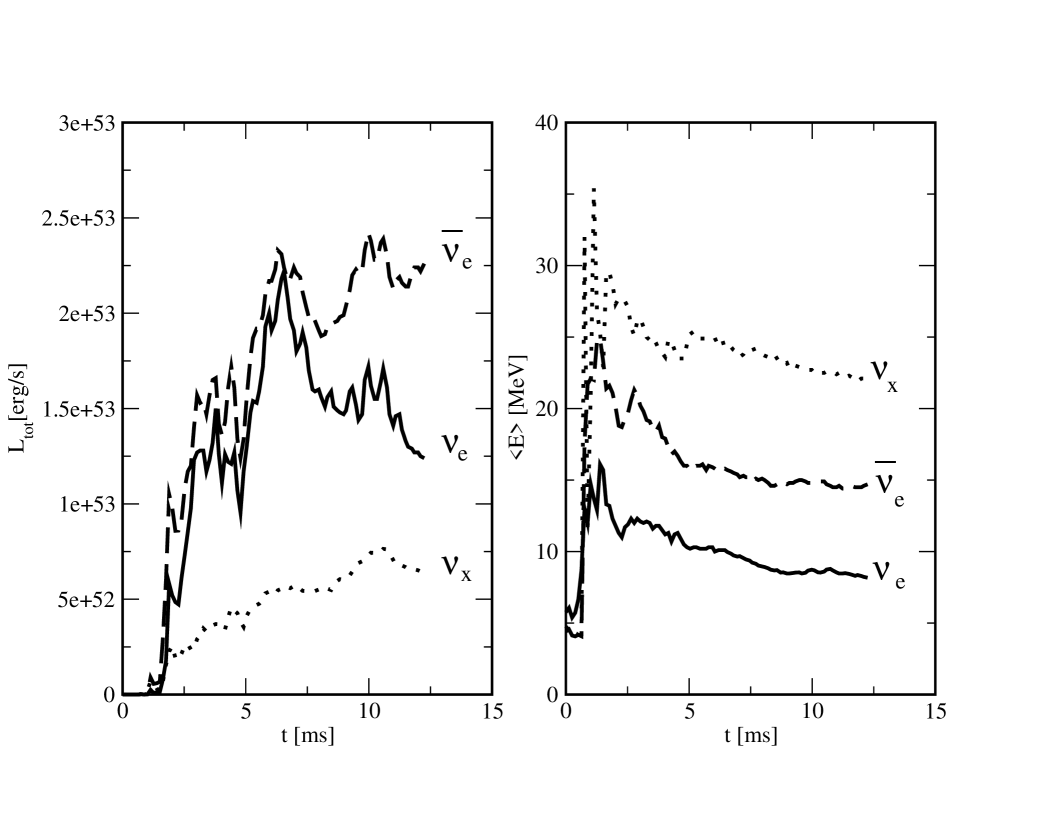
Figure 4: Run E (no spins, 2 x 2.0 ${\rm M_{\odot}}$): the left panel shows the luminosities (in ergs/s) of the different neutrino flavours. The right panel gives the corresponding mean energies. We regard this to be an upper limit for the neutrino emission.

         

         

         

Figure 8: End of run C (2 x 1.4 ${\rm M_{\odot}}$, no spins): logarithm of the optical depths (in steps of 0.5) of the various neutrino flavours calculated on our grid. The first panel shows $\nu_{e}$, the second $\bar{\nu}_{e}$ and the third $\nu_{x}$. The thick lines give the locus of the “neutrino sphere” defined as $\tau_{\nu_{i}}=$ 2/3, which is essentially the locus where the neutrinos decouple from the debris matters. For the $\bar{\nu}_{e}$ and $\nu_{x}$ the neutrino spheres almost coincide since both are subject to scattering processes, the absorption of $\bar{\nu}_{e}$ onto protons is only a minor correction. $\nu_{e}$ are additionally absorbed in the neutron-rich environment. Therefore the corresponding neutrino sphere is substantially larger.

Figure 9: Same as Figure 8, but for the end of run D (corotation, 2 x 1.4 ${\rm M_{\odot}}$).

Figure 10: Same as previous plot for run E.

Figure 13: Cylindrical grid for neutrino opacities.

References

- [\citeauthoryearAbramovici, Althouse, Drever, Gursel, Kawamura, Raab, Shoemaker, Sievers, Spero & ThorneAbramovici et al.1992] Abramovici A., Althouse W. E., Drever R. W. P., Gursel Y., Kawamura S., Raab F. J., Shoemaker D., Sievers L., Spero R. E., Thorne K. S., 1992, Science, 256, 325
- [1] Arnett, W. D. 1967, Canadian J. of Phys., 215, 1621
- [2] Arnett, W. D. 1977, ApJ, 218, 815
- [\citeauthoryearAyal, Piran, Oechslin, Davies & RosswogAyal et al.2001] Ayal S., Piran T., Oechslin R., Davies M. B., Rosswog S., 2001, ApJ, 550, 846
- [3] Balsara D., 1995, J. Comput. Phys., 121, 357
- [4] Baron E., Cooperstein J., & Kahana, S. 1985, Phys. Rev. Lett., 55, 126
- [\citeauthoryearBaumgarte, Cook, Scheel, Shapiro & TeukolskyBaumgarte et al.1997] Baumgarte T., Cook G., Scheel M., Shapiro S., Teukolsky S., 1997, Phys. Rev. Lett., 79, 1182
- [5] Benz W., 1990, in Buchler J., ed., Numerical Modeling of Stellar Pulsations. Kluwer Academic Publishers, Dordrecht, p. 269
- [6] Benz W., Bowers R., Cameron A., Press W., 1990, ApJ, 348, 647
- [7] Bethe, H. A. & Wilson, J. R. 1985, ApJ, 295, 14
- [8] Bildsten, L. & Cutler, C., 1992, ApJ, 400, 175
- [9] Bowers, R. L. & Wilson, J. R. 1982, ApJS, 50, 115
- [\citeauthoryearBradaschia et al.Bradaschia et al.1990] Bradaschia C. et al., 1990, Nucl.Instrum. Methods Phys. Res. A, 289, 518
- [10] Bruenn, S.W., 1985, ApJS, 58, 771
- [11] Bruenn, S. W., DeNisco, K. R., & Mezzacappa, A. 2001, ApJ, 560, 326
- [12] Burrows, A., Hayes, J., & Fryxell, B. A. 1995, ApJ, 450, 830
- [13] Burrows, A., Young, T., Pinto, Ph., Eastman, R. & Thompson, T. A. 2000, ApJ, 539, 865
- [14] Burrows, A., Thompson, T. A., Pinto, Ph. 2002, astro-ph/0211194
- [15] Colgate, S. A. & White, R. H. 1966, ApJ, 143, 626
- [16] Cooperstein, J., van den Horn, L. J., Baron, E. A., 1986, ApJ, 309, 653
- [\citeauthoryearDanzmannDanzmann1997] Danzmann K., 1997, in of Sciences T. N. Y. A., ed., Proceedings of the 17th Texas Symposium on relativistic astrophysics and cosmology New York
- [17] Eichler D., Livio M., Piran T. & Schramm D.N., 1989, Nature 340, 126
- [\citeauthoryearFaber & RasioFaber & Rasio2000] Faber J., Rasio F., 2000, Phys.Rev. D62, p. 064012
- [\citeauthoryearFaber, Rasio & ManorFaber et al.2001] Faber J., Rasio F., Manor J., 2001, Phys.Rev. D63, p. 044012
- [18] Fryer, C. F. & Warren, M. S. 2002, ApJL, 574, 65
- [\citeauthoryearFreiburghaus, Rosswog & ThielemannFreiburghaus et al.1999] Freiburghaus C., Rosswog S., Thielemann F.-K., 1999, ApJ, 525, L121
- [19] Haft, M., Raffelt, G. & Weiss, A., 1994, ApJ, 425
- [20] Herant, M., Benz, W., & Colgate, S. A. 1992, ApJ, 395, 642
- [21] Herant M., Benz W., Hix R. W., Fryer C. L., & Colgate, S. A. 1994, ApJ, 435, 339
- [22] Itoh, N., Nishikawa, A. & Kohyama, Y., 1996, ApJ, 470, 1015
- [23] Janka, H.-T. & Müller, E. 1996, A&A, 306, 167
- [24] Janka, H.-T., Kifonidis, K., & Rampp, M. 2001, in Proc. Workshop on Physics of Neutron Star Interiors, ed. D. Blaschke, N. Glendenning, & A. Sedrakian, Lecture Notes in Physics (Germany: Springer), 333
- [25] Kluzniak, W. & Ruderman, 1998, ApJ, 508, L113
- [26] Kochanek, C.S., 1992, ApJ, 398, 234
- [\citeauthoryearKuroda et al.Kuroda et al.1997] Kuroda K. et al., 1997, in Gravitational Wave Detection, Proceedings of the TAMA International Workshop on Gravitational Wave Detection held at National Women’s Education Centre, Saitama, Japan, on 12-14 November, 1996. Edited by K. Tsubono, M.-K. Fujimoto, and K. Kuroda. Frontiers Science Series No. 20. Universal Academy Press, Inc., 1997., p.309 Japanese gravitational wave observatory (jgwo). pp 309+
- [27] Lai, D. 1994, MNRAS, 270, 611
- [\citeauthoryearLattimer & SchrammLattimer & Schramm1974] Lattimer J. M., Schramm D. N., 1974, ApJ, (Letters), 192, L145
- [\citeauthoryearLattimer & SchrammLattimer & Schramm1976] Lattimer J. M., Schramm D. N., 1976, ApJ, 210, 549 Inc.)
- [28] Liebendörfer, M., Mezzacappa, A., Thielemann, F.-K., Messer, O. E. B., Hix, W. R., & Bruenn, S. W. 2001, Phys. Rev., D63, 103004
- [29] Liebendörfer, M., Messer, O. .E. B., Mezzacappa, A., Bruenn, S.W., Cardall, C.Y., Thielemann, F.K., 2002, submitted to ApJS, astro-ph/0207036
- [30] Lyford, N.D., Baumgarte, T.W., Shapiro, S.L., 2002, to appear in ApJ, gr-qc/0210012
- [31] Mezzacappa, A. & Bruenn, S. W. 1993, ApJ 405, 669
- [32] Mezzacappa, A., Calder, A. C., Bruenn, S. W., Blondin, J. M., Guidry, M. W., Strayer, M. R., & Umar, A. S. 1998, ApJ, 495, 911
- [33] Mezzacappa, A. & Messer, O. E. B. 1999, JCAM, 109, 281
- [34] Mezzacappa, A., Liebendörfer, M., Messer, O. E. B., Hix, W. R., Thielemann, F.-K., & Bruenn, S. W. 2001, PRL, 86, 1935
- [35] Monaghan J.J., 1992, Ann. Rev. Astron. Astrophys., 30, 543
- [36] Morris J., Monaghan J.J., 1997, J. Comp. Phys., 136, 41
- [37] Myra, E. S., Bludman, S. A., Hoffman, Y., Lichtenstadt, I., Sack, N., & Van Riper, K. A. 1987, ApJ, 318, 744
- [Narayan et al.(1992)] Narayan R., Paczyński B., Piran T., 1992, ApJ, 395, L83
- [\citeauthoryearOechslin, Rosswog & ThielemannOechslin et al.2001] Oechslin R., Rosswog S., Thielemann F.-K., 2002, Phys. Rev. D, 65, 103005
- [\citeauthoryearOohara & NakamuraOohara & Nakamura1997] Oohara K., Nakamura T., 1997, in Relativistic Gravitation and Gravitational Radiation. Cambridge University Press, Cambridge
- [Paczyński(1986)] Paczyński B., 1986, ApJ, 308, L43
- [38] Pons, J. A., Reddy, S., Prakash, M., Lattimer, J. M., & Miralles, J. A. 1999, ApJ, 513, 780
- [39] Rampp, M. & Janka, H. T. 2000, ApJL, 539, L33
- [\citeauthoryearRosswog, Liebendörfer, Thielemann, Davies, Benz & PiranRosswog et al.1999] Rosswog S., Liebendörfer M., Thielemann F.-K., Davies M. B., Benz W., Piran T., 1999, A & A, 341, 499
- [40] Rosswog S., Davies M. B., Thielemann F.-K., Piran T., 2000, A & A, 360, 171
- [Rosswog & Davies 2002] Rosswog S., Davies M. B., 2002, MNRAS, 334, 481
- [Rosswog & Ramirez-Ruiz E. 2002] Rosswog S., Ramirez-Ruiz E., 2002, MNRAS, 336, L7
- [\citeauthoryearRuffert, Janka & SchäferRuffert et al.1996] Ruffert M., Janka H., Schäfer G., 1996, A & A, 311, 532
- [Ruffert et al. 1997a] Ruffert M., Janka H.-T., Schäfer G., 1997, A & A, 311, 532
- [Ruffert & Janka 2001] Ruffert M., Janka H.-T., 2001, A & A, 380, 544
- [41] Schwartz, R. A. 1967, Ann. Phys., 43, 42
- [42] Shapiro,S. & Teukolsky, S.A., 1983, Black holes, White Dwarfs and Neutron Stars, (New York) Whiley & Sons
- [43] Shen H., Toki H., Oyamatsu K., Sumiyoshi K., 1998a, Nuclear Physics, A 637, 435
- [44] Shen H., Toki H., Oyamatsu K., Sumiyoshi K., 1998b, Prog. Theor. Phys., 100, 1013
- [\citeauthoryearShibataShibata1999] Shibata M., 1999, Phys. Rev. D, 60, 104052
- [\citeauthoryearShibata & UryuShibata & Uryu2000] Shibata M., Uryu K., 2000, Phys. Rev. D, 61, 064001
- [\citeauthoryearShibata & UryuShibata & Uryu2002] Shibata M., Uryu K., 2002, Prog. Theor. Phys., 2002, 107, 265 356, 559
- [\citeauthoryearSymbalisty & SchrammSymbalisty & Schramm1982] Symbalisty E. M. D., Schramm D. N., 1982, Astrophys. Lett., 22, 143
- [45] Takahashi, K., El Eid, M.F. & Hillebrandt, W., 1978, A&A, 67, 185
- [46] Taylor, J.H., 1994, Rev. Mod. Phys., 66, 711
- [47] Thompson, T.A., Burrows, A. & Horvath, J.E., 2000, Phys. Rev. C, 62, 03580
- [48] Thompson, C. and Duncan, R.C., 1993, ApJ, 408, 194
- [49] Thompson, C., 1994, MNRAS, 270, 480
- [50] Thompson, T.A., Burrows,A., Meyer, B.S., 2001, ApJ, 562, 887
- [51] Thorsett, S.E. & Chakrabarti, D., 1999, ApJ, 512, 288
- [52] Tubbs, D.L. & Schramm, D.N., 1975, ApJ, 201, 467
- [53] Van Riper, K. A. 1979, ApJ, 232, 558
- [54] Van Riper, K. A., & Lattimer, J. M. 1981, ApJ, 249, 270
- [55] Wilson, J. R. 1971, ApJ, 163, 209
- [56] Wilson, J. R. 1985, in Numerical Astrophysics, ed. by Centrella, J. M., LeBlanc, J. M., & Bowers, R. L. (Boston: Jones and Bartlett)
- [\citeauthoryearWilson et al.Wilson et al.1996] Wilson J. R., Mathews G., & Marronetti, P. 1996, Phys. Rev. D, 54, 1317