The Dynamical Evolution of Black Hole-Neutron Star Binaries in General Relativity: Simulations of Tidal Disruption

Abstract

We calculate the first dynamical evolutions of merging black hole-neutron star binaries that construct the combined black hole-neutron star spacetime in a general relativistic framework. We treat the metric in the conformal flatness approximation, and assume that the black hole mass is sufficiently large compared to that of the neutron star so that the black hole remains fixed in space. Using a spheroidal spectral methods solver, we solve the resulting field equations for a neutron star orbiting a Schwarzschild black hole. The matter is evolved using a relativistic, Lagrangian, smoothed particle hydrodynamics (SPH) treatment. We take as our initial data recent quasiequilibrium models for synchronized neutron star polytropes generated as solutions of the conformal thin-sandwich (CTS) decomposition of the Einstein field equations. We are able to construct from these models relaxed SPH configurations whose profiles show good agreement with CTS solutions. Our adiabatic evolution calculations for neutron stars with low-compactness show that mass transfer, when it begins while the neutron star orbit is still outside the innermost stable circular orbit, is more unstable than is typically predicted by analytical formalisms. This dynamical mass loss is found to be the driving force in determining the subsequent evolution of the binary orbit and the neutron star, which typically disrupts completely within a few orbital periods. The majority of the mass transferred onto the black hole is accreted promptly; a significant fraction ($\sim 30\%$) of the mass is shed outward as well, some of which will become gravitationally unbound and ejected completely from the system. The remaining portion forms an accretion disk around the black hole, and could provide the energy source for short-duration gamma ray bursts.

I Introduction

The infall of compact objects into black holes (BHs) is of considerable interest in many branches of astrophysics. In particular, many of the arguments that can be made about coalescing neutron star-neutron star (NSNS) binaries also apply to coalescing black hole-neutron star (BHNS) binaries. Both are strong candidates for the central engines of short-duration gamma ray bursts (GRBs), since the merger timescale following tidal disruption is comparable to the GRB duration and the gravitational binding energies provide the characteristic energy scales inferred by observers Janka et al. (1999); Rosswog (2005a). It is possible that any ejected matter may contribute significantly to the r-process elemental abundance of the universe Freiburghaus et al. (1999); Rosswog et al. (1999, 2004). Additionally, they are expected to be among the most important sources of gravitational waves (GWs) that can be detected by both terrestrial laser interferometers such as LIGO Abbott and The LIGO Science Collaboration (2005), VIRGO Acernese and the VIRGO collaboration (2005), GEO Smith and the GEO 600 collaboration (2004), and TAMA Ando and the TAMA collaboration (2002), as well as the proposed space-based interferometer LISA Danzmann and the LISA study team (1996).

The key difference between the sources that can be observed with LIGO (and comparable detectors) and LISA is the characteristic frequency of the GW emission: LISA’s characteristic frequency range falls within $10^{-4}-10^{-1}~{}{\rm Hz}$, whereas LIGO operates between $10-500~{}{\rm Hz}$. Because of this, LIGO is most sensitive to the mergers of stellar-mass BHs, whereas LISA will observe more massive merging systems that involve either intermediate mass BHs (IMBHs), $M_{\rm BH}=10^{2}-10^{4}M_{\odot}$, or supermassive BHs (SMBHs), $M_{\rm BH}>10^{5}M_{\odot}$. The formation history leading to these encounters is likely to involve completely different processes.

Compact binaries with stellar-mass BHs are likely to be formed through typical stellar binary evolution, at rates that depend on parameters such as the binary mass ratio distribution, common-envelope efficiency, and the physics of supernova kicks, all of which remain somewhat uncertain (see Kalogera et al. (2001); Belczynski et al. (2002); Voss and Tauris (2003) and references therein for a thorough review). The mass distribution of BHs in such systems is poorly constrained, as none have been observed to date, but may vary widely, spanning a range $2M_{\odot}<M_{\rm BH}<25M_{\odot}$ Belczynski et al. (2004). For sufficiently tight binaries, merger will occur within a Hubble time. In these cases, the dissipative effects of gravitational radiation will cause the orbit to circularize as the binary separation shrinks, so that the eccentricity of the orbit is expected to be almost zero by the time the binary enters the LIGO band. Whether or not the compact object is tidally disrupted by its BH companion, as well as where this would occur in the latter case with respect to the Innermost Stable Circular Orbit (ISCO), depends on both the compaction of the compact object and the mass ratio (see Section II).

This simple picture does not apply to compact objects orbiting BHs with considerably higher mass. Both IMBHs and SMBHs are expected to reside within stellar clusters, whose dynamics will be determined by both stellar-BH and stellar-stellar gravitational encounters (scattering). Some stars will typically be scattered, either strongly or weakly, into the “loss cone”, i.e., the volume of phase space encompassing orbits with sufficiently small periastrons that the star will be tidally disrupted before being kicked into another orbit by future encounters (see Shapiro (1985) for a review of the original derivations, and Sigurdsson (2003); Merritt and Poon (2004) for more recent work). As a result, most objects that enter the loss cone do so at very high eccentricity, with periastron distances of $5-50$ Schwarzschild radii Freitag (2003a); Hopman and Alexander (2005). In many cases, these systems will approach the BH with eccentricities $e\gtrsim 0.1$ Barack and Cutler (2004).

GW detections from coalescence with higher mass BHs may yield very little information about the physics of NS matter, for the case of a NS falling into an IMBH, or any compact object (BH, NS, or white dwarf) falling into an SMBH with $M\gtrsim 10^{6}M_{\odot}$. These objects should plunge through the ISCO of the BH intact, since the tidal-disruption radius lies within the ISCO, and will likely be swallowed whole by the BH. For the opposite case, applicable to white dwarfs (WD) falling into IMBHs (and NSs into stellar-mass BHs), tidal disruption will occur outside the ISCO, a process we describe in detail in Sec. II.

For the vast majority of its lifetime, a stellar-mass compact object binary will inspiral very slowly, such that it can be described by a point-mass, post-Newtonian (PN) treatment. PN formalisms for the adiabatic inspiral epoch are now completely determined up to 3.5PN order Blanchet et al. (2004), and include lowest-order spin-orbit and spin-spin terms Kidder (1995); Will (2005). Once finite-size and tidal effects become important at close separation, it becomes necessary to solve the fully nonlinear Einstein field equations. Quasi-equilibrium binary configurations in circular orbits have been calculated in GR for NSNS Baumgarte et al. (1997, 1998); Bonazzola et al. (1999); Gourgoulhon et al. (2001); Shibata and Uryu (2001); Duez et al. (2002); Taniguchi and Gourgoulhon (2002), BHNS (see Baumgarte et al. (2004), hereafter BSS; Taniguchi et al. (2005a), hereafter TBFS, and references therein), and BHBH binaries (Cook (1994); Baumgarte (2000); Gourgoulhon et al. (2002); Yo et al. (2004a); for a thorough review of the topic and references, see Cook (2000); Baumgarte and Shapiro (2003)). Details of the transition from slow inspiral to rapid plunge, and deviations from the point-mass energy versus frequency relation found in quasi-equilibrium sequences, may yield important information about the physical parameters of the NS equation of state (EOS; see, e.g., Baumgarte et al. (1997); Ori and Thorne (2000); Faber et al. (2002)). It has been suggested Hughes (2002) that a combination of $~{}10-50$ broadband and narrowband observations of NSNS mergers might be able to constrain the NS radius to within a few percent. We will show below that BHNS mergers may be just as interesting, but it is likely that the interpretation of physical features in the GW signal will be significantly more complicated, since differences between stable and unstable modes of mass transfer may lead to radically different scenarios.

Eventually, for those systems in which the tidal limit is reached before the ISCO, mass transfer onto the BH will begin. This process is fundamentally dynamic in nature, and can only be modeled accurately by relativistic, three-dimensional hydrodynamic calculations. Attempts have been made to model these systems analytically, but as we will show below, the conclusions rely on a number of unphysical assumptions. The earliest work describing mass transfer in detail for compact object binary mergers Clark and Eardley (1977) assumed that mass transfer in NSNS binaries would conserve both mass and orbital angular momentum, and that both NSs would remain on a quasi-circular orbit in corotation during the evolution; a similar set of assumptions was used to describe BHNS binaries as a possible source of gamma-ray bursts Portegies Zwart (1998). A more complex treatment developed in Davies et al. (2005) drops the assumption of circularity, since it is not seen to hold in numerical calculations (e.g., Rosswog et al. (1999)). Still, their model for the evolution of BHNS systems undergoing mass transfer depends on a number of ad hoc assumptions that need to be tested by dynamical calculations in order to be proven valid.

Beyond uncertainties about the form of the late-inspiral GW signal produced by a BHNS merger, there remains the question of the event rate, which remains uncertain given the complete lack of detection of such systems to date. Still, it is possible to estimate the likely merger rate using population synthesis models, which can be calibrated against the observed galactic NSNS binary population and supernova rates. Recent estimates predict an advanced LIGO annual detection rate of anywhere from a few mergers Voss and Tauris (2003) up to potentially several hundred Belczynski et al. (2002).

Should a BHNS binary merger be observed, it might reveal a great deal about the physics of matter at nuclear densities. In particular, the onset of mass transfer would yield a clear indication about the NS radius, and, as we will explain in detail below, the stability of the mass transfer would yield important information as to the nuclear EOS. Whereas for NSNS binaries the characteristic frequencies of GW emission during the merger and formation of a remnant (either a hypermassive NS or BH) will typically occur at frequencies outside the peak sensitivity of even an advanced LIGO detector, the same is not true for BHNS binaries. Since the frequency at the onset of instability scales roughly inversely with the total binary mass, we expect stellar-mass BHNS mergers to occur at characteristic frequencies at which LIGO will be most sensitive, $\sim 100-500~{}{\rm Hz}$. If the GW signal from a merger was observed to be coincident with a short-duration gamma-ray burst, we could potentially determine their distance, luminosity, and characteristic beaming angle Kobayashi and Mészáros (2003). A detailed theoretical understanding of these systems is now more urgent than ever, in light of the recent localizations of short GRB afterglows Bloom et al. (2005); Gehrels et al. (2005); Covino et al. (2005); Fox et al. (2005); Berger et al. (2005); Retter et al. (2005), the first ever for these systems (many long-duration GRBs have been localized, but are believed to be the result of collapsing stars, not merging compact binaries).

Unfortunately, the current state-of-the-art for hydrodynamic calculations of BHNS inspiral and merger is far behind that for NSNS mergers. Calculations of the latter have been performed using a variety of Newtonian, PN, and relativistic gravitational formalisms (see, Rasio and Shapiro (1999); Baumgarte and Shapiro (2003) for thorough reviews, and Faber et al. (2004), hereafter FGR, for a more recent summary). Many calculations have now been performed in either the conformal flatness (CF) approximation to general relativity (GR) Faber et al. (2004); Oechslin et al. (2002), or in full GR Shibata and Uryū (2000, 2002); Shibata et al. (2003, 2005). These GR calculations now include sophisticated treatments of the NS EOS and physically appropriate initial spins (Shibata et al. (2005); NSs are expected to be nearly irrotational in the inertial frame, since the viscous timescale is much longer than the inspiral timescale, see Bildsten and Cutler (1992); Kochanek (1992) and Sec. II below).

The key difficulty that must be overcome to perform simulations of relativistic BHNS mergers is the same one that arises in the study of BHBH binaries; the presence of a spacetime singularity inside the black hole. To avoid encountering the singularity in a numerical simulation, the BH interior is excised from the computational grid in most current applications. This is justified by the fact that no information can propagate from the BH interior to the exterior, so the exterior can be evolved independently of the interior. While progress has been reported, especially very recently Pretorius (2005), black hole evolution calculations have been plagued by numerical instabilities. In some ways, BHNS mergers are even more difficult to evolve consistently, since both the singular behavior of the BH as well as the hydrodynamic nature of the NS must be confronted. Whereas the BHBH problem involves a pure vacuum solution of the Einstein field equations, the NS must always be evolved in such a way that the relativistic fluid is treated properly.

As a result of these difficulties, all hydrodynamic calculations performed to date of stellar-mass BHNS mergers have used Newtonian or quasi-Newtonian gravitational treatments Lee and Kluzniak (1995); Lee and Kluźniak (1999a, b); Lee et al. (2001); Kluźniak and Lee (2002); Janka et al. (1999); Rosswog et al. (2004). Needless to say, binaries containing a BH can be evolved accurately only by using relativistic hydrodynamics in a relativistic spacetime. We emphasize here that this applies both to the tidal field created by the BH, as well as the self-gravity of the NS. Previous Newtonian calculations have in some cases Lee and Kluźniak (1999b); Kluźniak and Lee (2002) used an approximate black hole potential, suggested in Paczynski and Wiita (1980), that creates an ISCO at $6M_{\rm BH}$, but no single static potential can generate the full set of relativistic forces experienced by matter in the strong-field regime. Calculations employing a fixed background BH metric have typically been performed for stars undergoing a tidal interaction with a massive BH, rather than a stellar-mass BH, with relativistic dynamical terms but a Newtonian treatment of the self-gravity. The secondary, in fact, is often assumed to be a white dwarf or main-sequence star. These models include SPH treatments without self-gravity Laguna et al. (1993), and both PPM Frolov et al. (1994) and spectral method Marck et al. (1996) treatments with Newtonian self-gravity. More recently, SPH techniques have been devised that evolve the NS matter in the background metric of a stellar-mass BH, using Newtonian-order correction to model the NS self-gravity, for both SPH Rasio et al. (2005); Bogdanovic et al. (2005) and characteristic gravity Bishop et al. (2005). This approach is appropriate for describing main-sequence stars or white dwarfs. However, since the tidal disruption is a result of a competition between the black hole tidal force and stellar self-gravity, this approach is not sufficient to describe BHNS binaries accurately. Modeling tidal disruption in BHNS binaries requires a relativistic treatment of both the black hole and the neutron star.

Here, we will make use of the CF approximation to GR, introduced by Isenberg Isenberg (1978) and Wilson and collaborators Wilson et al. (1996). The CF approximation amounts to assuming that the spatial metric remains conformally flat, so that the gravitational fields can be found by solving the constraint equations of GR, decomposed in the conformal thin-sandwich (CTS) decomposition York, Jr., (1999), alone. The CTS formalism has been used in numerous applications to construct initial data describing both NSNS and BHNS binaries in quasiequilibrium Baumgarte et al. (1997, 1998); Duez et al. (2002); Shibata and Uryu (2001); Gourgoulhon et al. (2001); Bonazzola et al. (1999); Taniguchi and Gourgoulhon (2002); Baumgarte et al. (2004); Taniguchi et al. (2005a). For these initial data the choice of a conformal background metric is completely consistent with Einstein’s initial value (constraint) field equations, although different choices may describe the astrophysical situation at hand more or less accurately. The situation is different for dynamical simulations in the CF approximation (e.g. Wilson et al. (1996); Oechslin et al. (2002); Faber et al. (2004); Dimmelmeier et al. (2005); Villain et al. (2004)), since the assumption that the spatial metric remains conformally flat is no longer strictly consistent with Einstein’s field evolution equations. For many applications, however, CF provides an excellent approximation. For spherically symmetric configurations, as an example, the CF approach is exact, and for many other applications the error has been shown to be in the order of at most a few percent (see, e.g., Cook et al. (1996)). It is particularly useful for exploring dynamical behavior, e.g., collapse or tidal break-up, which occurs on dynamical timescales and is unaltered by secular effects like gravitational radiation-reaction.

In this paper we present the dynamical extension of BSS, who calculated the first relativistic, quasiequilibrium BHNS sequences as solutions of the CTS decomposition of the Einstein field equations. Modifying their code to treat the metric for the Schwarzschild BH in isotropic (CF) coordinates, rather than the Kerr-Schild coordinates reported in BSS, we take their corotating quasiequilibrium configurations as initial data. As in BSS, we assume an extreme mass ratio, $M_{\rm BH}\gg M_{\rm NS}$, which allows us to hold the BH position fixed and restrict the computational grid to a neighborhood of the NS, thereby avoiding complications arising in the BH interior. We also assume a polytropic equation of state for the neutron star, as well as synchronous rotation. The resulting dynamical calculations are the first of their kind to solve the CTS field equations for the spacetime around the NS self-consistently by treating both the NS and BH relativistically. They allow us to study details of the dynamical mass-transfer process, particularly its stability. The CF approximation holds a stable equilibrium configuration constructed in the CTS formalism in strict dynamical equilibrium. Our calculation is a prototype of more detailed general relativistic calculations we hope to provide in the future that will involve irrotational NS models with more realistic EOSs and compactions, arbitrary mass ratios, and a fully self-consistent treatment of the spatial metric.

In the CF approximation, gravitational radiation reaction must be added in by hand in order to drive the system toward merger. While it is the secular energy losses to gravitational radiation that initially drive the binary system toward the point of tidal disruption, they play a much reduced role in the dynamics thereafter. Indeed, while secular forces determine the path the binary takes prior to merger, the merger itself is a fundamentally dynamical process, as we discuss in great detail below.

Our work is organized as follows. In Sec. II we discuss the important physical scales that define our problem, and present a detailed treatment of the traditional picture for determining the stability of mass transfer. We then discuss the limitations of this model, and explain why it may not be applicable for BHNS mergers. In Sec. III we describe our numerical methods, including the details of both our implementation of the CF field equations as well as our use of smoothed particle hydrodynamics (SPH) techniques to evolve the fluid configuration. In Sec. IV we compare our relaxed initial data to previous quasiequilibrium models, and find that we can construct configurations that satisfy the field equations to high accuracy while reproducing previous results. In Sec. V we present our simulations of merging binaries for different models of the NS polytropic EOS. Finally, in Sec. VI we discuss our results in the context of GW astrophysics, and describe our plans for further calculations.

II Physical Overview

The evolution of binaries containing NSs is a fully relativistic problem, since lowest-order PN approximations break down in the strong gravitational fields present during late stages of the merger. However, we can use information from Newtonian and quasi-Newtonian calculations to estimate the various timescales and physical regimes we expect to encounter. Thus, we first classify the relevant physical scales we expect to encounter in our study of BHNS binary evolution, and then generalize the standard model for stable, binary mass transfer to relativistic stars. In doing so, we will explain why this model, variants of which have been used previously to describe the evolution of compact binaries, is unlikely to apply to BHNS mergers.

Our simple mass-transfer model does have physical relevance, as it can apply to the case of a WD inspiraling in a nearly circular fashion toward an IMBH in a globular cluster. Such a star will begin transferring mass long before reaching the ISCO. However, since WDs are typically kicked into highly eccentric orbits prior to interactions with the BH, the orbit may not have time to circularize fully before the onset of mass transfer. In such cases, the binary evolution will be more complicated than the scenario we consider here; it has been studied before by several groups (see Sigurdsson (2003); Rathore et al. (2005), and references therein).

II.1 Units, Timescales and Characteristic Lengths

The four most important timescales characterizing the problem at hand are the NS dynamical timescale $t_{D}$, the viscous timescale $t_{v}$, the orbital timescale $T$, and the GW radiation-reaction timescale $t_{\rm GW}$. Throughout this paper, we set $G=c=1$. The BH and NS masses can be written in terms of the initial mass ratio $q$ as $M_{\rm BH}=q^{-1}M_{\rm NS}$ or equivalently $M_{\rm NS}=qM_{\rm BH}$, and the NS radius $R_{\rm NS}={\cal C}^{-1}M_{\rm NS}=q{\cal C}^{-1}M_{\rm BH}$, where ${\cal C}\equiv M_{\rm NS}/R_{\rm NS}$ is the compactness parameter.

The dynamical timescale of the NS is given by

$$t_{D}\equiv\sqrt{\frac{2R_{\rm NS}^{3}}{M_{\rm NS}}}=2^{1/2}{\cal C}^{-1.5}M_{\rm NS}=2^{1/2}q{\cal C}^{-1.5}M_{\rm BH}.$$ (1)

We wish to compare this with the orbital and radiation-reaction timescales at the radius where Roche-lobe overflow will begin. To estimate this radius, we will use the approximate form proposed in Paczyński (1971),

$$R_{r}=0.46a\left(\frac{q}{1+q}\right)^{1/3},$$ (2)

which gives the (volume-averaged) Roche-lobe radius as a function of the mass ratio and binary separation $a$, for a binary treated as a pair of point masses in the corotating frame. This definition differs from the original definition of the Roche lobe, which was defined for incompressible matter (point masses are in effect infinitely compressible), but the physical scalings are the same; the coefficient becomes $0.41$ for incompressible matter instead of $0.46$. The Roche-lobe radius is equal to the NS radius at a separation

$$a_{R} = 2.17q^{-1/3}(1+q)^{1/3}{\cal C}^{-1}M_{\rm NS}$$ (3)

$$= 2.17q^{2/3}(1+q)^{1/3}{\cal C}^{-1}M_{\rm BH},$$

at which point the (Keplerian) orbital period is

$$T\equiv 2\pi\sqrt{\frac{a_{R}^{3}}{M_{T}}} = 20.1(1+q)^{1/2}{\cal C}^{-1.5}M_{\rm NS}$$ (4)

$$= 20.1q(1+q)^{1/2}{\cal C}^{-1.5}M_{\rm BH}\sim 14t_{D},$$

where $M_{T}\equiv M_{\rm NS}+M_{\rm BH}$ is the total binary mass, and the last relation holds for $q\ll 1$, or equivalently, $M_{T}\simeq M_{\rm BH}$. We note that in this limit, the orbital period is a fixed multiple of the NS dynamical timescale, regardless of the properties of the NS.

For a point-mass binary on a circular orbit, lowest order radiation reaction predicts that the binary will inspiral, losing energy and angular momentum, on a characteristic timescale $t_{\rm GW}$ given by

$$t_{\rm GW}=\frac{a}{\dot{a}}=\frac{E}{\dot{E}}=\frac{J}{2\dot{J}}=\frac{5}{64}\frac{a^{4}}{M_{\rm NS}M_{\rm BH}M_{T}}=4\tau,$$ (5)

where $\tau$ is the coalescence time, i.e., the remaining time until the point-mass binary would reach $a=0$. At the Roche-lobe separation, assuming $q\ll 1$, we have

$$t_{\rm GW} = 1.73q^{2/3}{\cal C}^{-4}M_{\rm NS}$$ (6)

$$= 1.73q^{5/3}{\cal C}^{-4}M_{\rm BH}=1.23q^{2/3}{\cal C}^{-5/2}t_{D}.$$

In general, the radiation-reaction timescale will be at least an order of magnitude longer than the dynamical timescale for any binary which begins mass transfer outside the ISCO radius. The orbital period $T$, however, may become similar to the coalescence time $t_{\rm GW}$, indicating that the infall becomes quite rapid.

In Fig. 1, we show the regions in parameter space for which the critical separation for Roche-lobe overflow lies within or outside of the ISCO, for a wide variety of compact object-BH binaries. Dashed vertical lines correspond to the approximate compactness of either a WD or a NS, whereas dotted horizontal lines show the approximate mass ratios to be expected for a $10M_{\odot}$ stellar-mass BH, an IMBH, or a SMBH. Systems above the critical curve reach the tidal limit before the ISCO, and are likely to transfer mass onto the BH. For those sufficiently below the curve, we expect that the compact object will pass through the ISCO intact, and plunge onto the BH relatively intact.

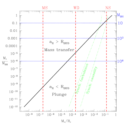
Figure 1: The critical mass ratio $q=M_{*}/M_{\rm BH}$ as a function of the secondary’s compaction ${\cal C}=M_{*}/R_{*}$, for which mass transfer begins at the ISCO, taken here as $a=6M_{\rm BH}$ (solid line). For systems above the curve, mass transfer begins while the orbit is stable; for those below, the secondary may plunge into the BH before being tidally disrupted. Dashed vertical curves show characteristic compactions of a WD or NS; dotted horizontal curves show typical mass ratios for a $1M_{\odot}$ compact object orbiting a $10M_{\odot}$ stellar-mass BH, a $10^{3}M_{\odot}$ IMBH, or a $10^{6}M_{\odot}$ SMBH. Dot-dashed curves show where $\beta$, the ratio of the light crossing time the viscous timescale of the NS, equals unity, and where $\alpha_{\rm Vis}$, the nondimensional turbulent viscosity assumes its largest reasonable value for the turbulent viscosity [See Eqs. (7) and (9)]. Only configurations to the left of these curves can synchronize prior to merger.

We note however, that this simple picture may very well be altered by a number of more complicated effects. Recently, Miller Miller (2005) has argued that even if systems are expected to reach the mass-shedding limit prior to crossing the ISCO, in many cases they will have already begun to plunge. Indeed, since the binary energy as a function of separation flattens out significantly near the ISCO, $t_{GW}$, which is already nearly of order $T$, will systematically underestimate the infall velocity (a similar argument was used in Faber et al. (2002) to argue that the GW energy spectrum produced in NSNS mergers declines dramatically near the ISCO). Because of this, the ISCO may systematically underestimate the binary separation at which prompt merger becomes inevitable.

On the other hand, describing the “plunge” of an extended object like a NS may provide a misleading picture of the dynamical merger in cases where the tidal disruption occurs inside the ISCO but outside the horizon. While it is certain that some matter, likely a significant fraction of the NS mass, will plunge inward directly onto the BH, this may liberate a great deal of angular momentum into the outer parts of the NS Rosswog (2005b). As a result, some fraction of the mass may survive the plunge, at least initially, in the form of a “mini-NS”, which will escape outside the ISCO on an elliptical orbit. Needless to say, only dynamical calculations will clarify the role played by these competing effects.

The final timescale we must consider is the viscous damping timescale $t_{\rm Vis}$, which we expect to play a crucial role in determining the fate of the binary once mass transfer commences. In the limit that the viscous timescale is extremely short (high viscosity), we expect two important phenomena to occur. First, tidal dissipation can synchronize the binary so that the secondary is corotating upon the onset of mass transfer. From Bildsten and Cutler (1992), we note that a binary will be synchronized by the time mass transfer begins only if

$$\beta\equiv\frac{R_{\rm NS}}{t_{\rm Vis}} \gtrsim 60(1+q)^{5/3}q^{-2/3}{\cal C}^{3},$$ (7)

$$t_{\rm Vis} \lesssim \frac{1}{60}(1+q)^{-5/3}q^{2/3}{\cal C}^{-4}M_{\rm NS}$$ (8)

$$\lesssim \frac{1}{60}(1+q)^{-5/3}q^{5/3}{\cal C}^{-4}M_{\rm BH},$$

where $\beta$ is the ratio of the light crossing time of the secondary to its viscous timescale, as defined by Bildsten and Cutler (1992). If we follow Duez et al. (2004) and assume that turbulent viscosity is the primary damping mechanism, we can define $\alpha_{\rm Vis}$, the turbulent viscosity parameter, so that

$$\alpha_{\rm Vis}\equiv\frac{t_{D}}{t_{\rm Vis}}.$$ (9)

We see that synchronization will occur if

$$\alpha_{\rm Vis}\gtrsim 60(1+q)^{5/3}q^{-2/3}{\cal C}^{5/2}.$$ (10)

On Fig. 1, we show curves marking the critical mass ratio-compactness dependence for $\beta=1$, which we define as the “causal limit”, as well as for $\alpha_{\rm Vis}=0.1$, which is the maximum plausible value for turbulent viscosity in physical systems of interest Balbus and Hawley (1998). Configurations to the left of the curve can synchronize before merger; this includes essentially all mergers where the secondary is either an MS star or a WD. NS mergers, on the other hand, will be irrotational in general, especially when the primary is a BH, since the required viscosity to synchronize the NS increases as the primary mass increases Bildsten and Cutler (1992); Kochanek (1992). Viscosity should also play a role after mass transfer starts, as we will discuss in detail below.

II.2 The stability of mass transfer

Once the secondary fills its Roche lobe, it will begin to transfer mass onto its companion. Such a process can be either stable or unstable, depending on its response to mass loss. If the volume of the Roche lobe shrinks faster than (or expands slower than) the stellar radius, the process is unstable, and the star will typically be disrupted violently. On the other hand, if a small amount of mass loss causes the star to shrink back within the Roche lobe, it is possible for the mass loss to temporarily cease, or at the very least settle down to a much smaller equilibrium level, whose value can be determined based on the assumptions made about conservation of mass and angular momentum, as we discuss below.

We first note that models of stable mass transfer typically assume that the binary orbit remains quasicircular, which in turn is only possible if the viscous timescale is short relative to the orbital and GW timescales. Maintaining a circular orbit requires that the orbital energy evolve according to a fixed relation in terms of the orbital angular momentum and the mass of the secondary, but there is no reason to assume that such a relation should hold a priori. Indeed, it is viscous dissipation that drives the orbit toward circularity, by converting excess orbital energy into other forms. Furthermore, when the viscous timescale is long, the mass-transfer rate can grow extremely rapidly, since the inner Lagrange point travels into the secondary at roughly $v_{in}R_{NS}/a_{R}$, unbinding progressively denser material from the NS. If this leads to an unstable runaway, it is the mass loss that drives the orbital evolution, and we expect to find the development of an orbital eccentricity. This violates the typical assumptions made in conservative mass-transfer models, which assume that mass loss is steady, and slow enough that the orbit can remain circular as mass is lost.

The early attempt to follow the mass transfer process in detail for NSNS binaries was provided by Clark and Eardley (1977), who modeled the heavier NS as a point mass, and the lighter secondary using an EOS that yields a nearly flat mass-radius relation down to $M_{\rm NS}\sim 0.3M_{\odot}$, below which the NS begins to expand rapidly with further decreasing mass. Rather than assume conservative mass transfer, they parameterized the possible loss of both mass and angular momentum from the system, finding that the former has very little effect on their results. In their model, mass transfer leads to a widening of the binary orbit, under the condition that the NS radius must equal the radius of its Roche lobe. As mentioned above, this will only hold for systems in which $t_{\rm Vis}\ll t_{\rm GW}$. Over time, the mass loss rate and GW luminosity decrease rapidly from their large initial values at closest approach (as does the rate of neutrino production as the NS matter decompresses during the transfer), until eventually the low-mass NS begins to expand rapidly Colpi et al. (1989) and unstable mass transfer begins.

Many of these ideas were revisited for a discussion of BHNS binaries in Portegies Zwart (1998), in light of the optical identification of GRB counterparts at cosmological distances. Assuming a Newtonian $n=1.5$ polytropic EOS and fully conservative mass transfer, they find that the initial mass-transfer rate between a $1.4M_{\odot}$ NS and a BH with mass $M_{\rm BH}=3-5M_{\odot}$ will occur at a rate of $\sim 100M_{\odot}{\rm s}^{-1}$ for approximately $1~{}{\rm ms}$ before decaying away according to the approximate power-law relation $\dot{M}_{\rm NS}\propto t^{-14/11}$, which corresponds to $M_{\rm NS}(t)\propto t^{-3/11}$. As in Clark and Eardley (1977), they assume that the process will terminate when the NS reaches a critical minimum mass and begins to expand unstably.

The most recent treatment of BHNS coalescence makes a completely different set of assumptions about the dynamics during mass transfer. Based on the Newtonian BHNS numerical calculations of Rosswog, Speith, and Wynn Rosswog et al. (2004), Davies, Levan, and King Davies et al. (2005) assume that the rapid timescale for mass transfer will violate the assumption of circular orbits, which underlies the typical conservative, quasiequilibrium mass-transfer formulation. Instead, they make the following assumptions:

1. Mass transfer occurs during a timescale corresponding to half an orbit.

2. During this time period, the NS, treated as a uniform density sphere, will lose mass from a shell whose depth is a distance equivalent to the infall rate from the beginning of the mass-transfer rate multiplied by half an orbital period.

3. Half of the angular momentum lost to the transferred mass will return to the NS, placing it on an eccentric orbit that will typically not lead to overflow during the next periastron passage.

This model does reproduce well the extremely high mass loss rates initially seen during Newtonian numerical calculations of BHNS mergers Lee and Kluźniak (1999a); Janka et al. (1999); Rosswog et al. (2004), but the assumptions adopted are somewhat ad hoc. In particular, transferring angular momentum back to the NS without adjusting its mass causes a discontinuous evolution of the binary orbit. In some cases, the NS will find itself on an orbit whose periastron is outside the mass-shedding limit, leading to a period of stable evolution until GW dissipation forces the orbit to decay inward again back to the onset of mass transfer. In contrast, we find below that mass transfer can be quenched temporarily, but from this point on the NS follows an elliptical trajectory that will take it back within the mass-shedding limit prior to the next periastron passage.

In Appendix A, we derive a semi-analytic formulation for conservative mass transfer onto a BH, modeling secondaries either by a Newtonian or a relativistic polytrope. We recover the scaling relations found in Clark and Eardley (1977); Portegies Zwart (1998), and generalize them for arbitrary polytropic indices. Although these relations are unlikely to hold for merging BHNS systems, as shown in Fig. 1, the Newtonian results can be applied to merging WDs as well as main sequence stars undergoing mass transfer. We note that there are semi-analytic formalisms for describing non-conservative mass transfer as well (see, e.g. Podsiadlowski et al. (1992) for a formalism involving mass transfer from a main sequence star onto a companion), and that these have been useful in describing WDBH mergers Fryer et al. (1999), but that the actual NS tidal disruption process is sufficiently dynamic that essentially all analytic treatments break down.

The theory of accretion disk dynamics presents several interesting connections to that of merging binaries, since questions about the stability of mass transfer appear as well (see, e.g., Daigne and Font (2004) and references therein). One key difference between the models is the typical radial angular momentum distribution; parameterizing the tangential velocity profile as $v_{t}(r)\propto r^{\alpha}$, irrotational NS have a nearly flat velocity profile, $\alpha\sim 0$, and corotating NS a flat angular velocity profile, $\alpha=1$, both larger than the Keplerian value $\alpha_{K}=-0.5$. Moreover, NS differ greatly from disks because of their infall velocity when they pass through the ISCO, and their strong self-gravity. While angular momentum distributions with larger values of $\alpha$ help to stabilize mass transfer in disks, stronger self-gravity destabilizes mass transfer Daigne and Font (2004). Thus, it is hard to generalize across the classes, although we note that irrotational NS should, if anything, be more prone to unstable mass transfer, as the NS loses more angular momentum per unit mass lost from its inner edge.

III Numerical techniques

To compute the dynamical evolution of a BHNS binary, we fix the position of the BH and assume that the surrounding spacetime metric takes the form appropriate to a nonspinning Schwarzschild BH. The approximation of a fixed BH position is correct in the limit that $M_{\rm BH}\gg M_{\rm NS}$. Here, we will study binaries with mass ratios $q\equiv M_{\rm NS}/M_{\rm BH}=0.1$, which is presumably within the range of values for which the approximation of an extreme mass ratio is valid.

To calculate gravitational forces and evolve the fluid configuration, we will work within the CF formalism, which we explain in more detail in Section III.2 below. We assume that the spatial metric is remains conformally flat, so that it can be written in the form

$$ds^{2}=(-\alpha^{2}+\beta_{k}\beta^{k})dt^{2}+2\beta_{i}dx^{i}dt+\psi^{4}\delta_{ij}dx^{i}dx^{j},$$ (11)

where $\alpha$ and $\beta^{i}$ are the lapse function and shift vector, respectively. Under this assumption we only need to solve the $3+1$ constraint equations for $\psi$, $\alpha$ and $\beta^{i}$ to determine the metric.

Our initial configuration places the NS in a corotating initial configuration. Irrotational configurations, which are more realistic astrophysically, will be treated in a later publication. We model the NSs as relativistic polytropes, and assume adiabatic evolution, which we describe in detail in Sec. III.1.

The code we use both to relax and evolve BHNS binaries is similar to that introduced in FGR Faber et al. (2004) for evolving NSNS binaries. We solve the five linked non-linear field equations of the CF formalism, Eqs. (24), (25), and (26) below, using the LORENE libraries, publicly available at http://lorene.obspm.fr. These Poisson-like equations are solved using spectral methods, decomposing the fields and their sources in a set of radially distinct domains into radial and angular expansions. Dynamical evolution is treated through SPH discretization. Many aspects of the code were discussed in detail in FGR, so we concentrate instead on the changes and new features introduced to evolve BHNS binaries.

Roughly speaking, we have made three significant changes to the code to admit the presence of a BH in the binary. First, the asymptotic Schwarzschild BH contribution to the spacetime metric is held fixed, allowing us to solve the field equations describing the self-gravity of the NS in a fully consistent way. Second, as discussed below, we solve Poisson-like elliptic equations for $\psi$ and $(\alpha\psi)$, as in BSS and elsewhere, rather than for $\nu\equiv\ln\alpha$ and $\beta\equiv\ln(\alpha\psi^{2})$, as in FGR and related treatments (TBFS denotes the latter quantity “$\sigma$”). Third, we restrict the spatial domain of our spectral methods field solver to a finite radius centered on the NS, as was done in BSS and TBFS, which allows us to avoid problems near the BH. Indeed, our computational domain is chosen so as not to overlap the event horizon at any time. As a result, we do not make use of the asymptotic boundary conditions typically used by LORENE-based codes, which can be extended to spatial infinity through the proper coordinate transformations Bonazzola et al. (1998). The use of a restricted spatial domain has been introduced before, in the context of domains with ingoing and outgoing GWs Novak and Bonazzola (2004), but with a set of BC’s that are not appropriate to the (elliptic) problem at hand. Instead, as we describe below, we have introduced a multipole expansion BC, used here and in TBFS, which should be more accurate than the lowest-order power-law falloff conditions traditionally used in grid-based calculations. Below, we first summarize the relevant equations that comprise relativistic hydrodynamics (Sec. III.1) and the CF formalism (Sec. III.2), introduce the “split” equations which factor out the BH contributions to the spacetime in Sec. III.3, describe our new approach for introducing a multipole BC in Sec. III.4, and finally describe how this affects the evaluation of various quantities in the SPH evolution equations Sec. III.5.

III.1 Relativistic Hydrodynamics

We assume that the matter can be described as a perfect fluid so that the stress-energy tensor takes the form

$$T^{\mu\nu}=\rho_{0}(1+\varepsilon+\frac{P}{\rho_{0}})u^{\mu}u^{\nu}+Pg^{\mu\nu},$$ (12)

where $\rho_{0}$, $\varepsilon$, $P$, and $u^{\mu}$ denote the rest mass density, specific internal energy, pressure, and 4-velocity, respectively. We will describe the NS by a relativistic polytropic EOS that evolves adiabatically with index $\Gamma$. Hence, the pressure obeys the relation

$$P=(\Gamma-1)\rho_{0}\varepsilon,$$ (13)

and initially satisfies

$$P=\kappa\rho_{0}^{\Gamma},$$ (14)

where $\kappa$ is a constant. As discussed in BSS, we can scale away dimensional units by setting $\kappa=1$ (see their Sec. IIIc).

The Lagrangian continuity equation (FGR,Oechslin et al. (2002)) can be written as

$$\frac{d\rho_{*}}{dt}+\rho_{*}\partial_{i}v^{i}=0$$ (15)

where we define the conserved density

$$\rho_{*}\equiv\alpha u^{0}\psi^{6}\rho_{0}=\gamma_{n}\psi^{6}\rho_{0},$$ (16)

and the coordinate velocity

$$v^{i}=\frac{u^{i}}{u^{0}}=-\beta^{i}+\frac{u_{i}}{u^{0}\psi^{4}},$$ (17)

and introduce the Lorentz factor for the fluid $\gamma_{n}\equiv\alpha u^{0}$. Lagrangian time derivatives are related to Eulerian partial time derivatives through the familiar relation $d/dt\equiv\partial/\partial t+v^{i}\partial_{i}$. To determine the Lorentz factor, we solve the normalization condition for the 4-velocity,

$${\gamma_{n}}^{2}=(\alpha u^{0})^{2}=1+\frac{u_{i}u_{i}}{\psi^{4}}=1+\frac{\tilde{u}_{i}\tilde{u}_{i}}{\psi^{4}}\left[1+\frac{\Gamma\kappa\rho_{*}^{\Gamma-1}}{(\gamma_{n}\psi^{6})^{\Gamma-1}}\right]^{-2},$$ (18)

implicitly.

The Euler equation can be written

$$\frac{d\tilde{u}_{i}}{dt}=-\frac{\alpha\psi^{6}}{\rho_{*}}\partial_{i}P-\alpha hu^{0}\partial_{i}\alpha+\tilde{u}_{j}\partial_{i}\beta^{j}+\frac{2h\alpha(\gamma_{n}^{2}-1)}{\gamma_{n}\psi}\partial_{i}\psi,$$ (19)

where the specific momentum is defined by

$$\tilde{u}_{i}\equiv hu_{i},$$ (20)

and the specific enthalpy $h$ by

$$h\equiv 1+\Gamma\varepsilon.$$ (21)

Finally, the energy equation takes the form

$$\frac{de_{*}}{dt}+e_{*}\partial_{i}v^{i}=0,$$ (22)

where $e_{*}=\gamma_{n}\psi^{6}(\rho_{0}\varepsilon^{\Gamma-1})^{1/\Gamma}$. For an adiabatic evolution without shock heating, the energy equation is satisfied automatically by adopting Eq. (14).

To account for shocks, we included an artificial viscosity prescription composed of both linear and quadratic terms (the relativistic analogue of the form introduced in Hernquist and Katz (1989), similar to that found in Oechslin et al. (2002)). We found no evidence for significant shocks within the body of the NS, as only the matter in the mass transfer stream directed toward the BH showed signs of significant heating very near the BH. Using the value of $\kappa\equiv P/\rho_{0}^{\Gamma}\equiv(\Gamma-1)\varepsilon/\rho_{0}^{\Gamma-1}$ as a measure, a quantity that remains constant during an adiabatic evolution, we found variation of no more than $5\%$ within the body of the NS. This is hardly a surprise, as there is no physical mechanism such as a collision to cause significant shocking within the bulk of the NS. Shock heating will be important for understanding the evolution of the initially low-density accretion stream that falls toward the BH, especially near the event horizon. In this region, the heating can be substantial, but it seems not to introduce significant feedback on the NS remnant. Given these results, we replace the energy equation, Eq. (22), with its adiabatic solution, Eq. (14), throughout the calculations described here. In future calculations, where shocks may be more important, we will restore the full evolution of the energy equation with an artificial viscosity prescription and allow for shocks everywhere. This will be especially important for irrotational NS calculations, since the matter transferring through the inner Lagrange point has significantly greater angular momentum than in the irrotational case, and a great deal of it will likely forming a disk rather than accreting promptly.

III.2 The CF formalism

In the CF formalism Isenberg (1978); Wilson et al. (1996) we assume that the spatial metric is not only conformally flat initially, but that it remains conformally flat. In particular, for the 3-metric we approximate $\partial_{t}\tilde{\gamma}_{ij}=0$ so that in rectangular coordinates $\tilde{\gamma}_{ij}=\delta_{ij}$ at all times. Strictly speaking, this is inconsistent with Einstein’s evolution equations, but is often a very good approximation, particularly on dynamical timescales when secular motion due to radiation-reaction is not important. Under this approximation the evolution equation for the spatial metric yields a relation between the extrinsic curvature and the shift,

$$K_{ij}\equiv\frac{\psi^{4}}{2\alpha}\left[\delta_{il}\partial_{j}\beta^{l}+\delta_{jl}\partial_{i}\beta^{l}-\frac{2}{3}\delta_{ij}\partial_{l}\beta^{l}\right].$$ (23)

Inserting this expression into the momentum constraint yields an equation for the shift $\beta^{i}$

$$\nabla^{2}\beta^{i}+\frac{1}{3}\partial^{i}(\partial_{j}\beta^{j}) = 16\pi\alpha\psi^{4}(E+P)U^{i}$$ (24)

$$\!\!\!\!\!\!\!\!\!\!\!\!\!+2\alpha\psi^{4}K^{ij}\nabla_{j}(\ln[\alpha/\psi^{6}])\equiv S_{\beta}^{i},$$

where $\nabla^{2}$ is the flat space Laplacian. The Hamiltonian constraint is an equation for the conformal factor $\psi$

$$\nabla^{2}\psi=-2\pi\psi^{5}E-\frac{1}{8}\psi^{5}K_{ij}K^{ij}\equiv S_{\psi}.$$ (25)

To derive an equation for the lapse $\alpha$, the remaining undetermined function in the metric, Eq. (11), we choose maximal slicing $K\equiv\gamma^{ij}K_{ij}=0$ at all times, which implies $\partial_{t}K=0$. This choice can be combined with the evolution equation for the extrinsic curvature, which then yields

$$\nabla^{2}(\alpha\psi)=2\pi\alpha\psi^{5}(E+2S)+\frac{7}{8}\alpha\psi^{5}K_{ij}K^{ij}\equiv S_{\alpha\psi}.$$ (26)

In the above equations the matter sources $E$, $S$ and $U^{i}$ are projections of the stress-energy tensor $T_{\mu\nu}$ and can be expressed as

$$E = \rho_{0}h\gamma_{n}^{2}-P,$$ (27)

$$S = 3P+\frac{\gamma_{n}^{2}-1}{\gamma_{n}}(E+P),$$ (28)

$$U^{i} = \frac{\tilde{u}_{i}}{\gamma_{n}h\psi^{4}}.$$ (29)

In practice, it is easier to decompose the three coupled equations for the shift, Eq. (24), into four decoupled Poisson equations. To do so, we follow Oohara et al. (1997); Shibata et al. (1998) and define

$$\beta^{i}=4B_{i}-\frac{1}{2}[\partial_{i}(\chi+B_{k}x^{k})]=\frac{7B_{i}-\partial_{i}\chi-x^{k}\partial_{i}B_{k}}{2},$$ (30)

and solve the set

$$\nabla^{2}B_{i} = \frac{S_{\beta}^{i}}{4},$$ (31)

$$\nabla^{2}\chi = -\frac{S_{\beta}^{i}x_{i}}{4}.$$ (32)

These Poisson-like equations, found in Shibata et al. (1998) and elsewhere, are exactly equivalent to those found in FGR for $\nu\equiv\ln\alpha$ and $\beta\equiv\ln(\alpha\psi^{2})$, and share the same asymptotic fall-off behavior, but have radically different properties near the horizon of the BH, where the lapse function goes to zero. This causes divergences in the values of $\nu$ and $\beta$, whereas $\alpha$ and $\psi$ remain finite and easy to deal with in a numerical treatment. Our chosen variables also exhibit a slightly different behavior when we split them into additive pieces contributed largely by the NS and BH, i.e., the contributions from the NS and BH to $\psi$ and $\alpha\psi$ are additive, whereas the logarithmic dependence of the “$\nu-\beta$” set means that the two contributions are combined multiplicatively.

As several different sets of notation have now been introduced into the literature to define equivalent quantities in the CF formalism, we present alternate notations used in a selection of other works in Table 1.

Table 1: A comparison of our notation for various relativistic quantities to that found in a selection of previous works using the CF formalism: Faber et al. (2004); Gourgoulhon et al. (2001); Oechslin et al. (2002); Shibata et al. (1998); Wilson et al. (1996). For those cases where no unique terminology was defined, we give the simplest equivalent algebraic form.

Quantity	Here	FGR Faber et al. (2004)	Gourgoulhon Gourgoulhon et al. (2001)	Oechslin Oechslin et al. (2002)	Wilson Wilson et al. (1996)	Shibata Shibata et al. (1998)
Lapse	$\alpha$	$N$	$N$	$\alpha$	$\alpha$	$\alpha$
Shift	$\beta_{i}$	$-N_{i}$	$-N_{i}$	$\beta_{i}$	$\beta_{i}$	$\beta_{i}$
Conformal Factor	$\psi$	$\sqrt{A}$	$\sqrt{A}$	$\psi$	$\phi$	$\psi$
Rest Density	$\rho_{*}$	$\rho_{*}$	$\Gamma_{n}A^{3}\rho$	$\rho_{*}$	$D\phi^{6}$	$\rho_{*}$
Lorentz Factor	$\gamma_{n}$	$\gamma_{n}$	$\Gamma_{n}$	$\alpha u^{0}$	$W$	$\alpha u^{0}$
Velocity	$v^{i}$	$v^{i}$	$NU^{i}+N^{i}$	$v^{i}$	$V^{i}$	$v^{i}$
Specific Momentum	$\tilde{u}_{i}$	$\tilde{u}_{i}$	$w_{i}$	$\tilde{u}_{i}$	$S_{i}/(D\phi^{6})$	$\tilde{u}_{i}$
Enthalpy	$h$	$h$	$h$	$w$	$h$	$1+\Gamma\epsilon$

III.3 BHNS binaries

The CF approximation is exact for spherically symmetric configurations, reproducing the TOV equation for fluid configurations as well as the Schwarzschild solution for a stationary, non-spinning black hole. In isotropic coordinates, such a solution is given by

$$ds^{2}=-\left(\frac{1-M_{\rm BH}/2r}{1+M_{\rm BH}/2r}\right)^{2}dt^{2}+\left(1+\frac{M_{\rm BH}}{2r}\right)^{4}\delta_{ij}dx^{i}dx^{j}.$$ (33)

From this metric we identify the BH lapse and conformal factors as

$$\alpha_{{\rm BH}} = \frac{1-M_{\rm BH}/2r}{1+M_{\rm BH}/2r},$$ (34)

$$\psi_{{\rm BH}} = 1+\frac{M_{\rm BH}}{2r}.$$ (35)

The BH contribution to the shift $(\beta_{i})_{{\rm BH}}$, vanishes in isotropic coordinates (unlike in the Kerr-Schild coordinates used by BSS).

To convert this line element to the more familiar Schwarzschild (areal) coordinates, with

$$ds^{2}=-\left(1-\frac{2M_{\rm BH}}{\tilde{r}}\right)dt^{2}+\left(1-\frac{2M_{\rm BH}}{\tilde{r}}\right)^{-1}d\tilde{r}^{2}+\tilde{r}^{2}d\Omega^{2},$$ (36)

one makes the coordinate transformation

$$\tilde{r} = \left(1+\frac{M_{\rm BH}}{2r}\right)^{2}r,$$ (37)

$$r = \frac{1}{2}\left[\tilde{r}-M_{\rm BH}+\sqrt{\tilde{r}(\tilde{r}-2M_{\rm BH})}\right].$$ (38)

Note that this implies that the Schwarzschild radius and ISCO radius take the values

$$\tilde{r}=2~{}M_{\rm BH} \leftrightarrow r=0.5~{}M_{\rm BH},$$ (39)

$$\tilde{r}=6~{}M_{\rm BH} \leftrightarrow r=4.949~{}M_{\rm BH}.$$ (40)

At asymptotically large distances, $\tilde{r}=r+M_{\rm BH}$.

As discussed at length in Gourgoulhon et al. (2001), it is useful to “split” the field equations when dealing with binaries, so that the terms on the RHS of each equation are concentrated on either component of the binary. Here, the method is slightly different. Since the BH solution is an exact solution of the vacuum field equations, it can be subtracted out of the full metric field equations to yield the CF solution for the largely-NS contribution to the fields. Defining $N\equiv\alpha\psi$, and accordingly, $N_{\rm BH}\equiv\alpha_{\rm BH}\psi_{\rm BH}=1-M_{\rm BH}/{2r}$, we split the fields such that

$$\psi = \psi_{{\rm BH}}+\psi_{{\rm NS}},$$ (41)

$$\alpha = \alpha_{{\rm BH}}+\alpha_{{\rm NS}},$$ (42)

$$N\equiv\alpha\psi = N_{{\rm BH}}+N_{{\rm NS}}$$

$$\Rightarrow N_{{\rm NS}}=\alpha_{{\rm NS}}\psi_{{\rm NS}}+\alpha_{{\rm BH}}\psi_{{\rm NS}}+\alpha_{{\rm NS}}\psi_{{\rm BH}}.$$

The NS piece of the field equations, Eqs. (25) and (26), can be expressed as

$$\nabla^{2}\psi_{{\rm NS}} = -2\pi(\psi_{{\rm BH}}+\psi_{{\rm NS}})^{5}E$$ (44)

$$-\frac{1}{8}(\psi_{{\rm BH}}+\psi_{{\rm NS}})^{5}(K_{ij})_{{\rm NS}}(K^{ij})_{{\rm NS}},$$

$$\nabla^{2}N_{{\rm NS}} = 2\pi(N_{{\rm BH}}+N_{{\rm NS}})(\psi_{{\rm BH}}+\psi_{{\rm NS}})^{4}(E+2S)$$ (45)

$$\!\!\!\!\!\!\!\!\!\!\!\!\!\!\!\!\!\!\!\!\!\!\!\!+\frac{7}{8}(N_{{\rm BH}}+N_{{\rm NS}})(\psi_{{\rm BH}}+\psi_{{\rm NS}})^{4}(K_{ij})_{{\rm NS}}(K^{ij})_{{\rm NS}}.$$

The BH contributes to the shift vector, Eq. (24) only through the lapse function and conformal factor, since the black hole contribution to the shift vanishes in isotropic coordinates.

III.4 Multipole Boundary Conditions

The LORENE-based field solver we use decomposes the angular dependence of all scalar, vector, and tensor quantities into spherical harmonics (the radial decomposition into Chebyshev polynomials is described in detail in Bonazzola et al. (1998)). For configurations in which the outermost boundary extends to spatial infinity, the outer boundary condition can be set exactly to zero for any field which satisfies a power-law falloff. For a BHNS binary, however, that is not an option, since we encounter numerical difficulties when the computational domain overlaps the BH singularity. Instead, we must impose an approximate BC for each field on the outermost (spherical) boundary, which lies at a finite radius, as shown in Fig. (2). This outermost boundary is chosen so that it never overlaps the BH event horizon.

Any Poisson-like equation $\nabla^{2}\Phi=\rho$ with compact support has an exterior solution given by

$$\Phi(\tilde{r},\theta,\phi) = \sum_{l=0}^{\infty}\sum_{m=-l}^{l}\left[\int_{0}^{R}\rho r^{l}Y^{*}_{lm}(\theta,\phi)d^{3}\vec{r}\right]$$ (46)

$$\times Y_{lm}(\theta,\phi)\tilde{r}^{-(l+1)}$$

$$\equiv \sum_{l=0}^{\infty}\sum_{m=-l}^{l}\rho_{lm}Y_{lm}(\theta,\phi)\tilde{r}^{-(l+1)},$$

where we define the multipole moments of the source term $\rho_{lm}$ [see Eq. (4.2) of Jackson (1975)]. This solution established the boundary conditions for our outermost computational domain, and can be matched to the interior solutions to yield the field solution everywhere in space. Here, the source terms of the Poisson-like Eqs. (24), (25), and (26) are not compact, but instead satisfy rather steep power-law falloffs, allowing us to use the same formalism while introducing only small errors. Noting that the matter configurations are equatorially symmetric, we only sum over multipoles with the same equatorial symmetry as the particular field (i.e., $l+m$ even for $\psi$, $\alpha$, $\beta^{x}$, $\beta^{y}$, and $\chi$; $l+m$ odd for $\beta^{z}$). Rather than evaluate the real field source integrals against the complex spherical harmonics $Y_{lm}$, we evaluate both the multipole moments and the resulting expansions against the real and imaginary parts of the spherical harmonics $Y_{lm}$ with $m\geq 0$ (noting that $Y_{l0}$ are purely real and that $Y_{l,-m}=(-1)^{m}Y^{*}_{lm}$). Finally, we truncate the expansion at a predetermined value $l=l_{max}$, where throughout this paper we use $l_{max}=4$, or hexadecapole order. Thus, we assume $\rho_{lm}=0$ for all terms with $l>l_{max}$ when we define the BC’s for our field equations. This is done for two reasons. First, the multipole coefficients fall off steeply at high $l$, so that the higher order multipole make ever smaller contributions to the field at large separation. Second, including higher order multipoles can lead to purely numerical instabilities in the field solvers for a finite set of Chebyshev polynomials, since the rapid oscillations with respect to angle can lead to large gradients in derivative-based quantities.

We find that that a multipole treatment can lead to significantly higher accuracy for our boundary solution, at the cost of some computational efficiency. To avoid numerical instabilities arising from quickly growing higher-order multipoles, we employ underrelaxation during each iteration, updating each field such that $\psi_{new}=(1-\lambda)\psi_{old}+\lambda\tilde{\psi}_{new}$, where $\psi_{old}$ is the field value from the previous iteration, and $\tilde{\psi}_{new}$ is the new solution found from solving the elliptic equation. We find good stability and efficiency by setting $\lambda=0.5$ initially, and increasing the value to $\lambda=0.5-0.05\log(\Delta\beta^{y})$ with each iteration, where $\Delta\beta^{y}$ is the maximum relative change in the y-component of the shift vector from iteration. The iteration loop terminates when $\Delta\beta^{y}<10^{-9}$, at which point $\lambda\simeq 0.95$, representing very weak underrelaxation.

Our multipole BC’s allow us to calculate the forces on particles that fall outside the computational domain directly, since the multipole expansion for the metric is valid throughout space. Indeed, for such particles, we calculate the BH contribution to the lapse and conformal factor from Eqs. (34) and (35), the NS contribution from the multipole expansions given by Eq. (46), and the gradients of the NS contribution from

$$\frac{\partial\Phi}{\partial x^{i}} = \partial_{i}\sum_{l,m}\frac{r^{l}\rho_{lm}Y_{lm}}{r^{2l+1}}$$ (47)

$$= \sum_{l,m}\rho_{lm}\left[\frac{\partial_{i}(r^{l}Y_{lm})}{r^{2l+1}}-\frac{(2l+1)x^{i}r^{l}Y_{lm}}{r^{2l+3}}\right],$$

noting that $\partial r/\partial x^{i}=x^{i}/r$.

This works directly for the lapse and conformal factor, but the shift vector is slightly more complicated. Recall that we have solved elliptic equations not for $\beta^{i}$, but for $B_{i}$ and $\chi$, as defined in Eq. (30), and thus only know the multipole decomposition of the latter quantities. In terms of these, the gradient of the shift is given by

$$\partial_{j}\beta^{i}=\frac{7\partial_{j}B_{i}-\partial_{i}B_{j}-\partial_{i}\partial_{j}\chi-x^{k}\partial_{i}\partial_{j}B_{k}}{2},$$ (48)

where we also evaluate terms of the form

$$\frac{\partial^{2}\Phi}{\partial x^{i}\partial x^{j}} = \sum_{l,m}\rho_{lm}\left[\frac{\partial_{i}\partial_{j}(r^{l}Y_{lm})}{r^{2l+1}}\right.$$ (49)

$$\left.-\frac{2l+1}{r^{2l+3}}\left(x^{i}\partial_{j}(r^{l}Y_{lm})+x^{j}\partial_{i}(r^{l}Y_{lm})\right.\right.$$

$$~{}~{}~{}~{}~{}~{}~{}~{}~{}~{}~{}~{}\left.\left.+\delta_{ij}r^{l}Y_{lm}\right)\right.$$

$$\left.+\frac{(2l+1)(2l+3)x^{i}x^{j}r^{l}Y_{lm}}{r^{2l+5}}\right].$$

Since the lapse goes to zero at the horizon, particles approaching it become frozen in proper time, and cannot penetrate within.

The approach we use has several advantages over the leading order power-law falloff BC’s typically used in BSS and other grid-based field calculations (e.g., Shibata and Uryū (2002)). First, we lose less information about the source terms by extending to higher order multipoles (Shibata et al. (2003) include dipole order falloff terms for the lapse and conformal factor in full GR, while Oechslin et al. (2002) include quadrupole-order terms for these in CF gravity). Moreover, we avoid a problem associated with symmetries present in our quasi-equilibrium initial conditions which are broken during the dynamical evolution. In particular, as we show in Appendix B, our quasiequilibrium configurations can be shown to have a vanishing monopole contribution to $\beta^{x}$, and vanishing monopole and dipole contributions to $\beta^{z}$. Once the binary becomes tidally disrupted, however, we expect the monopole contribution to $\beta^{x}$ and the dipole contribution to $\beta^{z}$ to grow in magnitude ($\beta^{z}$ may never have a monopole contribution, since equatorial symmetry holds for dynamical configurations as well). While these terms are growing, we are faced with a situation where the leading-order term may very well not be the largest magnitude multipole contribution on the boundary. Defining a global power-law falloff index to fit the boundary condition. as in previous treatments, is impossible even when the two lowest-order moments are known, since the index varies with angle. Instead, our multipole summation handles this situation naturally, calculating all low-order moments accurately.

III.5 SPH Discretization, Computational Domains, and Timestepping

Many of the methods used to perform an SPH discretization of the CF hydrodynamic and field equations are discussed in FGR, so here we summarize briefly the fundamental aspects of the SPH treatment and the new features present in our BHNS code. The neighbor finding algorithms used in our code are based on routines from StarCrash, a publicly available, extensively documented Newtonian SPH code, which can be found online at www.astro.northwestern.edu/theory/StarCrash.

Motivated by the form of the Lagrangian continuity equation (15), we define the mass $m_{a}$ of each particle, fixed in time, in terms of the conserved density $\rho_{*}$, such that

$$(\rho_{*})_{a}=\sum_{b}m_{b}W_{ab},$$ (50)

where $W_{ab}$ is the ${\cal C}^{2}$, piecewise, “$W_{4}$” smoothing kernel function for a pair of particles introduced by Monaghan and Lattanzio (1985), and used in FGR and elsewhere. For each particle, we define a smoothing length $h_{a}$, and compute all sums over particles that lie within a sphere of radius $2h_{a}$ surrounding each particle (we calculate all SPH quantities using a “gather-scatter” technique, as described in FGR and the StarCrash documentation). Smoothing lengths are updated using underrelaxation in order to maintain a roughly constant number of neighbors for each particle, set at the beginning of each run. Each particle is advanced through space with a velocity $v^{i}=dx^{i}/dt$, which we evaluate with a second-order accurate leapfrog evolution scheme, calculating forces from the Euler equation (19) at the half-timestep. Since the calculation is adiabatic, the energy equation, Eq. (22) is automatically satisfied when we use the adiabatic EOS, Eq. (14). A typical timestep in our evolution scheme, started with particle velocities evaluated half a timestep in advance of the particle positions, involves a number of computational elements. First, we advance all particles a full timestep, and re-evaluate the particle neighbor lists and the SPH expressions for the density of each. We then use the SPH form for the density at each particle position to define the computational domains used by the Lorene field solver, shown schematically in Fig. 2. To do so, we calculate the position of the NS center of mass from all particles having a density $(\rho_{*})_{a}>\rho_{crit}$, where $\rho_{crit}$ is a critical value chosen to encompass the vast majority of particles at the beginning of a run. Next, we calculate the surface of the innermost computational domain $R_{1}(\theta,\phi)$, as the smallest triaxial ellipsoid, centered on the NS center of mass, that contains all particles that lie at greater radii from the BH than the NS center of mass, treating the particles as spheres of radius $2h_{a}$. This is very similar to the technique described in FGR, except that there we included all particles that passed the density cut, regardless of which side of the NS they fell within. Here, however, the dynamics of the mass transfer are different. In equal-mass NSNS binaries, the NS only begin to disrupt at very close separations, never deviating particularly far from an ellipsoidal configuration up to the point of merger. Here, mass transfer is initially one-sided toward the BH, and the outer half of the NS remains virtually intact while the inner half becomes deformed by the tidal gravity of the BH. We find that our field solver performs best if we define our elliptical domain based on the profile from the outer half of the NS, as it can handle without difficulty field sources located outside the innermost domain, but produces numerical errors if the density field of the NS drops to zero within the innermost domain. (see the second panel of Fig. 2). The two outer domains, which have the topology of spherical shells, are defined initially such that their outer boundaries are spheres at radii equal to twice and three times that of the maximum extent of the innermost shell, i.e. $R_{2}(\theta,\phi)=2\times\max(R_{1});R_{3}(\theta,\phi)=3\times\max[R_{1}]$. Over time, we hold the outermost boundary fixed at this radius, and adjust that of the second domain to be the geometric mean of the outer radius and the maximum value from the inner domain, i.e., $R_{2}=0.5*(R_{3}+\max[R_{1}])$ (compare the two panels of Fig. 2).

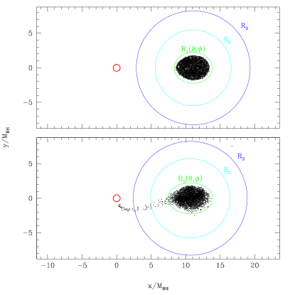
Figure 2: A schematic representation of the spectral methods computational domains used to solve the NS components of the field equations, Eqs. (25)-(24). Initially, a triaxial ellipsoid with surface $R_{1}(\theta,\phi)$ and origin at the NS center of mass is fitted around all SPH particles for which $(\rho_{*})_{i}>\rho_{crit}$ (top panel). Two annular “shell-like” domains with spherical outer boundaries are also laid down, with radii $R_{2}$ and $R_{3}$, twice and three times the maximum value of $R_{1}$. During the evolution (bottom panel), we use the same procedure to fit $R_{1}(\theta,\phi)$, keep the value of $R_{3}$ fixed, and calculate $R_{2}$ as the mean of $R_{3}$ and the maximum of $R_{1}$. Some particles first leave the innermost domain, and then the entire computational volume, particularly those accreted by the black hole, shown as a circle of radius $0.5~{}M_{\rm BH}$ centered at the origin.

Once the computational domains are defined, we use the techniques of Bonazzola et al. (1998) to define a set of “collocation points” at which we compute the local SPH expression for $\rho_{*}$, $\tilde{u}$, and $P_{*}\equiv\kappa\rho_{*}^{\Gamma}$, noting the latter remains equivalent to Eq. (13), for adiabatic evolution and polytropic initial data. From these, we calculate all other hydrodynamic quantities using the Lorene library routines, and solve the field equations iteratively. After every iteration of the field solver, all hydro quantities are updated to reflect the new fields.

Once a convergent solution is found, we must export back all relevant matter and field terms from the spectral decomposition to the particle positions. For particles in the innermost domain, we evaluate most hydrodynamical terms directly from the spectral decomposition. Thus, denoting by “SB” those terms evaluated in the spectral basis and “SPH” those quantities defined only on a particle-by-particle basis, we calculate the Euler equation as

$$\left(\frac{d\tilde{u}_{i}}{dt}\right)_{in} = [\alpha\psi^{6}]_{\rm SB}\left[\frac{\partial_{i}P}{\rho_{*}}\right]_{\rm SPH}$$ (51)

$$-\left[\alpha hu^{0}\partial_{i}\alpha+\frac{2h\alpha(\gamma_{n}^{2}-1)}{\gamma_{n}\psi}\partial_{i}\psi\right]_{\rm SB}$$

$$+\left[\partial_{i}\beta^{j}\right]_{\rm SB}[\tilde{u}_{j}]_{\rm SPH}.$$

This approach works in the outermost domains for extrinsic quantities like $\rho_{*}$ that go to zero smoothly at the surface of the NS matter, but fails for intrinsic quantities that have discontinuities there, , e.g., $u^{0}$ and $\gamma_{n}$, since the Chebyshev radial decomposition cannot describe discontinuous functions. Instead, we evaluate hydrodynamic terms for particles in these domains on a particle-by-particle basis, and evaluate field quantities and derivatives through the spectral decomposition,

$$\left(\frac{d\tilde{u}_{i}}{dt}\right)_{out} = [\alpha\psi^{6}]_{\rm SB}\left[\frac{\partial_{i}P}{\rho_{*}}\right]_{\rm SPH}$$ (52)

$$-[\alpha\partial_{i}\alpha]_{\rm SB}[hu^{0}]_{\rm SPH}$$

$$+\left[\frac{\alpha}{\psi}\partial_{i}\psi\right]_{\rm SB}\left[\frac{2h(\gamma_{n}^{2}-1)}{\gamma_{n}}\right]_{\rm SPH}$$

$$+\left[\partial_{i}\beta^{j}\right]_{\rm SB}[\tilde{u}_{j}]_{\rm SPH}.$$

After calculating the forces for the RHS of the Euler equation, we advance the velocities from their original half-timestep value forward to a half-timestep ahead of the positions, and then resolve the field equations to determine the velocity $v^{i}$ using the same approach described above for particles based upon their computational domain,

$$v^{i}=\left[\frac{1}{\psi^{4}u^{0}}\right]_{\rm SB}[\tilde{u}_{i}]_{\rm SPH}-[\beta^{i}]_{\rm SB},$$ (53)

in the innermost domain, with $u^{0}$ evaluated via SPH instead for the outer ones.

IV Equilibrium models

The first step in evolving BHNS binaries is the construction of accurate initial data. In our approach, this requires not only determining the fields and hydrodynamic quantities within and surrounding the NS, but also the construction of a relaxed SPH discretization configuration describing the NS itself.

We take as our starting point data constructed from the grid-based equilibrium scheme described in BSS. We modified the scheme of BSS to allow for a conformal background metric corresponding to a Schwarzschild BH in isotropic coordinates, which can be adopted more easily for the CF approximation used here, rather than the Kerr-Schild background used in BSS (see also TBFS). To construct an SPH particle decomposition, we first lay down a hexagonal close-packed lattice of SPH particles over the Cartesian coordinate volume where the density of the star is positive. Tentative particle masses are assigned to be proportional to the density $\rho_{*}$, normalized to match the proper NS mass. Next, we calculate the SPH value for the density of each particle, and adjust the masses and smoothing lengths of each particle until each has approximately the correct number of neighbors as well as the correct density, to within $\sim 2\%$. While the resulting configuration could serve as acceptable initial data, we can do better by evolving the configuration in the corotating frame with drag forces applied, to damp away spurious deviations from true equilibrium. This also allows us to relax to quasiequilibrium initial models with binary separations differing by up to $\sim 20\%$ in either direction using the same initial data from BSS. Of course, the new field solution will be different, reflecting the change in magnitude of the tidal terms, but we have found that after approximately 1000 timesteps of relaxed evolution, the overall level of spurious motion is equivalent.

We used two grid-base datasets to generate our initial data. For configuration A, the NS is modeled as a relativistic $\Gamma=1.5$ polytrope, of compaction $M_{\rm NS}/R_{\rm NS}=0.042$ (or equivalently, mass $\bar{M}_{\rm NS}=0.05$ orbiting a BH of mass $\bar{M}_{\rm BH}=10\bar{M}_{\rm NS}$ at a separation $a_{0}=11.8M_{\rm BH}$. Configuration B features a NS with the same compaction but a stiffer EOS, $\Gamma=2$ and $a_{0}=11.1M_{\rm BH}$ (where $\bar{M}$ is the dimensionless mass defined in Sec. IIIC of BSS). Note that in these units the maximum compaction of an isolated NS is $0.214$ and $0.074$ for adiabatic indices $\Gamma=2$ and $\Gamma=1.5$, respectively.

To convert from the units of BSS to those used here, many quantities must be linearly rescaled. In particular, for configuration A, $\bar{r}=10.5$, and $M_{\rm BH}=4.72$. Thus all distances should be multiplied by a factor $\bar{r}/M_{\rm BH}=2.2$ to convert from the “hatted” units of BSS to those here expressed in terms of the BH mass. Similarly, for configuration B, $\bar{r}=1.32$ and $M_{\rm BH}=0.5$, so the rescaling factor is $2.64$.

Both NS models are undercompact compared to the expected physical NS parameters. Since our method assumes an extreme mass ratio, we are limited to low compactness NS models in order to study cases where tidal disruption occurs outside the ISCO, as can be seen from Fig. 1. Thus, while our configurations do not exactly represent physical parameters expected to be found in BHNS binaries, they serve as an analogue to binaries containing lower-mass BHs and more compact NS that will have comparable tidal-disruption radii located outside the ISCO. In a future work, we will treat more physically realistic NS compactnesses, as well as NS spins, including cases for which the tidal-disruption radius is within the ISCO.

Below we describe the technique by which we generate our relaxed SPH initial conditions in Sec. IV.1, and then show the comparison between our resulting models and the grid-based data in Sec. IV.2.

IV.1 Relaxation of Initial Data

When preparing a fluid configuration to be evolved using SPH, it is generally necessary to use some form of relaxation first. Otherwise, numerical deviations from equilibrium present in the discretized initial configuration will drive the dynamics, leading to a variety of spurious effects. Relaxation is easiest to perform for configurations in which the matter will be stationary in some reference frame, such as a corotating system, since the spurious component of each particle’s velocity can be easily identified and damped away by a drag term in the force equation. This statement holds equally true for Newtonian and relativistic formalisms, although the latter require a slightly more complicated numerical treatment, for reasons we discuss below, primarily due to the presence of velocity-dependent forces as well as a more complicated set of variables used to define the equations of motion.

In order to derive the proper equations for a relaxation scheme in a relativistic setting, it is useful to start with a brief review of how the process works in Newtonian physics, and then generalize to the appropriate relativistic equation. In what follows, we define our coordinates such that the x-axis corresponds to the line connecting the centers of mass of the two objects, the y-direction to their orbital velocity, and the z-direction to the binary’s angular velocity.

In Newtonian physics, we have a set of inertial frame evolution equations

$$\frac{d\vec{r}}{dt} = \vec{v},$$ (54)

$$\frac{d\vec{v}}{dt} = \vec{a},$$ (55)

where the RHS of each are known functions used to define an initial condition. For the case of a corotating equilibrium binary configuration, these quantities take the form

$$\vec{v}_{eq} = \vec{\Omega}\times\vec{r},$$ (56)

$$\vec{a}_{eq} = -\Omega^{2}\vec{r}_{cyl},$$ (57)

where we use the subscript “eq” to indicate the relaxed value, and where $\vec{r}_{cyl}$ is the “cylindrical” radius. To evolve the fluid during the relaxation, we shift to the frame in which the matter is stationary. Thus we define

$$\vec{V}\equiv\vec{v}-\vec{v}_{eq}=\vec{v}-\vec{\Omega}\times\vec{r},$$ (58)

so that $\vec{V}=0$ for equilibrium configurations, and evolve $d\vec{x}/dt=\vec{V}$. We determine $\Omega$ as an eigenvalue from the condition that the binary center-of-mass separation is already known, by summing over all of our SPH particles. Based on symmetry considerations, only the x-component of the equation yields a non-trivial result:

$$\sum m_{i}\left(\frac{d\vec{V}}{dt}\right)^{x}_{i}=0 = \sum_{i}m_{i}\vec{a}^{x}_{i}-\sum_{i}m_{i}(\vec{a}_{eq})^{x}_{i}$$ (59)

$$= \sum_{i}m_{i}\vec{a}^{x}_{i}+\sum_{i}m_{i}\Omega^{2}x_{i},$$

which implies

$$\Omega=\sqrt{\frac{-\sum_{i}m_{i}\vec{a}^{x}_{i}}{\sum_{i}m_{i}x_{i}}}.$$ (60)

We add to the force equation a linear drag term with some characteristic timescale $\tau$ in order to damp away the spurious motion in of the initial condition. The relaxation timescale should generally be approximately equal to the dynamical time of the system. Thus, we evolve

$$\frac{d\vec{V}}{dt}=(\frac{d\vec{v}}{dt}+\Omega^{2}\vec{r}_{cyl})+\vec{a}_{drag}=\vec{a}+\Omega^{2}\vec{r}_{cyl}-\frac{\vec{V}}{\tau}.$$ (61)

As we approach equilibrium, both the term in parentheses as well as the drag term separately approach zero.

The relativistic case is slightly more complicated, but we can derive analogous relativistic expressions for all of our Newtonian ones. Our equations of motion now take the form

$$\frac{d\vec{x}}{dt} = \vec{v},$$ (62)

$$\frac{d\tilde{u}}{dt} = \vec{a},$$ (63)

where the velocity variables are related by Eq. (17), $\vec{v}=\tilde{u}/(\psi^{4}u^{0})-\vec{\beta}$. In a corotating frame in equilibrium, we know that $d(\psi^{4}u^{0})/dt=0$, and will treat the term as a constant. The shift vector has the time-dependence of the other vector quantities.

For a corotating configuration, we have

$$\vec{v}_{eq}=\vec{\Omega}\times\vec{r},$$ (64)

and the slightly more complicated Euler equation

$$\vec{a}_{eq}=\frac{d}{dt}[\psi^{4}u^{0}(\vec{v}+\vec{\beta})] = \psi^{4}u^{0}[\Omega\times(\vec{v}_{eq}+\vec{\beta})]$$ (65)

$$= \!\!\psi^{4}u^{0}[-\Omega^{2}\vec{r}_{cyl}+\Omega\times\vec{\beta}].$$

The matter will be propagated on trajectories with velocity $\vec{V}=\vec{v}-\vec{v}_{eq}$, just as before. Now, however, we have the condition

$$\vec{V}=\vec{v}-\vec{v}_{eq}=\frac{\tilde{u}}{\psi^{4}u^{0}}-\vec{\beta}-\vec{\Omega}\times\vec{r},$$ (66)

whose time derivative in equilibrium must satisfy the condition $\vec{a}_{eq}/(\psi^{4}u^{0})-\Omega\times\vec{\beta}+\Omega^{2}\vec{r}_{cyl}=0$. In the particle decomposition, we find

$$\sum m_{i}\left(\frac{dV^{x}}{dt}\right)_{i}=0 = \sum_{i}\frac{m_{i}a^{x}_{i}}{(\psi^{4}u^{0})_{i}}$$ (67)

$$+ \sum_{i}m_{i}\Omega\beta^{y}_{i}+\sum_{i}m_{i}\Omega^{2}x_{i}$$

$$= \sum_{i}\frac{m_{i}a^{x}_{i}}{(\psi^{4}u^{0})_{i}}$$

$$+ \!\!\!\!\Omega\sum_{i}m_{i}\beta^{y}_{i}+\Omega^{2}\sum_{i}m_{i}x_{i},$$

which can be solved for $\Omega$.

To the force equation, we also add a linear drag term with a characteristic timescale $\tau$, but the drag term must force $\tilde{u}$ toward its equilibrium value $\tilde{u}_{eq}=\psi^{4}u^{0}(\Omega\times\vec{r}+\vec{\beta})$, rather than toward zero, so that

$$\frac{d\tilde{u}}{dt}=\vec{a}-\vec{a}_{eq}-\frac{\tilde{u}-\tilde{u}_{eq}}{\tau} = \vec{a}+\psi^{4}u^{0}(\Omega^{2}\vec{r}_{cyl}-\Omega\times\vec{\beta})$$ (68)

$$- \frac{\tilde{u}-\psi^{4}u^{0}(\Omega\times\vec{r}+\vec{\beta})}{\tau}.$$

This equation should, barring any physical instabilities, damp away spurious motion and produce a corotating equilibrium configuration.

IV.2 Comparison with Other Quasi-Equilibrium Sequences

Our grid-based models, based on the scheme described in BSS but with isotropic background coordinates, were constructed using $48\times 48\times 24$ grids, with outer boundaries placed $\bar{x}=\pm 3,\bar{y}=\pm 3,\bar{z}=3$ for the $\Gamma=2$ case, and $\bar{x}=\pm 2,\bar{y}=\pm 2,\bar{z}=2$ for the $\Gamma=1.5$ case. SPH configurations were generated corresponding to these binary separations, as well as wider and narrower binary separations constructed by translating the NS to the appropriate position. The number of particles used to construct the SPH configurations were $n_{p}=103,953$ and $n_{p}=77,908$ for the $\Gamma=2$ and $\Gamma=1.5$ EOS, respectively. For the $\Gamma=1.5$ EOS configuration only particles of mass $m_{i}>10^{-4}m_{i;max}$ were accepted, where $m_{i;max}$ is the maximum mass of any SPH particle present. This mass cut is useful for eliminating an outermost layer of negligible total mass, which is typically blown off the surface of the NS anyway by even a tiny amount of spurious motion resulting from deviations from pure equilibrium in the initial condition.

Each SPH configuration was relaxed for 1000 time-steps, which corresponds to $\sim 10t_{D}$, a sufficient time given that the initial models were rather relaxed to begin with. Parameters for our grid-based models and the final SPH configurations at the end of relaxation are listed in Table 2. Models for $\Gamma=1.5$ are labeled A1 – A7, while models for $\Gamma=2$ are labeled B1 – B4. As a check, we compare the value of the period determined during the SPH relaxation process $T$, to the exact relativistic Kepler relation for a point mass about a BH, $T_{\rm N}\equiv\sqrt{\tilde{r}^{3}/M_{\rm BH}}$, and find very good agreement. Here the binary separation is measured in areal coordinates, whose relation to CF coordinates is given by (37).

We note that configurations A1-A3 do not settle down completely during relaxation. In each case, the central density of the NS dropped monotonically as the configuration expanded in the x-direction, indicating that mass transfer would eventually begin even with drag forces applied.

Table 2: Parameters for our relaxed initial models. $T_{\rm N}$ is the exact relativistic Keplerian period for a point mass about a BH, defined by Eq. (37).

Run	$a/M_{\rm BH}$	$\Omega M_{\rm BH}$	$T/M_{\rm BH}$	$T_{\rm N}/M_{\rm BH}$
	$\Gamma=1.5,q=0.1,{\cal C}=0.042$
A1	10.438	0.0258	243.8	243.8
A2	10.745	0.0247	254.0	253.7
A3	11.256	0.0232	270.6	270.3
A4	11.513	0.0225	279.1	278.8
A5	11.767	0.0218	287.5	287.3
A6	12.027	0.0212	296.5	296.1
A7	12.791	0.0194	323.1	322.5
	$\Gamma=2,q=0.1,{\cal C}=0.042$
B1	10.539	0.0255	246.4	247.0
B2	10.961	0.0242	260.2	260.7
B3	11.093	0.0238	264.6	265.0
B4	11.648	0.0222	283.0	283.3

In general, we find very good agreement between the grid-based initial data and our SPH configurations for stable configurations. In Fig. 3 and 4 we show a comparison between the field values and densities from our SPH configuration and the grid-based data along the x-axis, for configurations A5 and B3. In both cases the relevant fields agree to generally within about $1-2\%$. The only exception is configuration A5, where we find some disagreement between the two methods on the half of the NS facing the BH. The discrepancy is primarily due to the different BC’s: the grid based data imposes a $1/r$ power-law falloff condition on a cube whose inner edge is located at $\bar{x}=-2$, whereas the multipole solution used for the SPH configuration is imposed on a spherical boundary at $\bar{r}=4.5$. Thus, the spectral methods solution integrates over a much larger volume of space, and allows for higher-order terms in the field solution at the boundary, which are not insignificant at a distance corresponding to a few NS radii. The small disagreement in the density profile is in part an SPH effect: SPH typically smooths out the density field over each particle’s smoothing length. Since our particles are initially equally spaced along a lattice, this length is $\sim\delta\bar{x}=0.05$, and we cannot fully resolve the sharp density peak at the NS center.

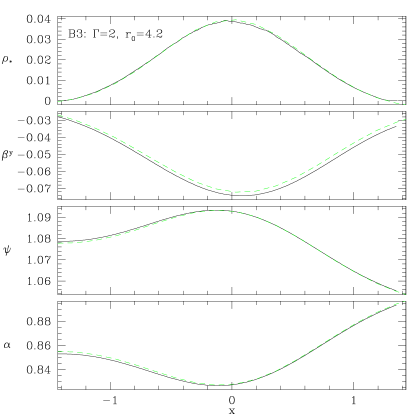
Figure 3: From top to bottom, the values of $\rho_{*}$, $\beta^{y}$, $\psi$, and $\alpha$ along the x-axis for the SPH (solid line) and grid-based (dashed line) data representing configuration B3, a NS with a $\Gamma=2$ polytropic EOS and an initial binary separation $a_{0}/M_{\rm BH}=11.1$. The agreement is generally to within $1-2\%$.

Figure 4: The values of $\rho_{*}$, $\beta^{y}$, $\psi$, and $\alpha$ along the x-axis for the SPH (solid line) and grid-based (dashed line) data representing configuration A5, a NS with a $\Gamma=1.5$ polytropic EOS and an initial binary separation $a_{0}/M_{\rm BH}=11.8$. Conventions are the same as Fig. 3.

We can formulate an independent check on the self-consistency of our initial data by checking how well they satisfy the integrated Euler equation,

$$\frac{h}{u^{0}}={\rm constant}.$$ (69)

This condition is typically used to generate initial data in grid-based calculations, e.g., Eq. (42) of BSS and Eq. (28) of TBFS, but appears nowhere in our relaxation scheme. As we show in Appendix C, it can be derived as a consequence of a relaxed initial configuration for which the RHS of the Euler equation (19) is zero. In Fig. 5 we show on a particle by particle basis the value of $h/u^{0}$, for configurations A5 and B3, plotted for clarity against the particle’s radial coordinate position outward from the NS center of mass. In both cases, we find the standard deviation from the mean is $<0.01\%$, and the maximum discrepancy $<0.1\%$.

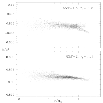
Figure 5: Value of the SPH expression for the integrated Euler equation constant $h/u^{0}$ as a function of the particle’s radius from the NS center of mass for configurations B3 (top) and A5 (bottom), featuring a NS EOS with $\Gamma=2$ and $\Gamma=1.5$, respectively. Note that the proper value differs between the two cases. The standard deviation in both cases is $<0.01\%$, with maximum variation $<0.1\%$.

V Evolution of BHNS binaries

From our relaxation results, it appears that the tidal disruption limit for the adopted choices of NS EOS would occur at binary separations $a_{0}/M_{\rm BH}\sim 11.0$, in line with the predictions of Eq. (2). For models with smaller binary separations, we were unable to find a convergent solution for the configuration with a stable central density maximum. These results can be confirmed through dynamical calculations in the strict CF formalism which ignore all energy and angular momentum losses from gravitational radiation-reaction. From our discussion in Sec. II.2, we might expect the possibility of qualitatively different behavior for NSs with the stiffer vs. softer EOS evolved from an initial configuration near the stability limit. For the softer EOS, we expect unstable mass transfer: the NS should disrupt completely once mass transfer begins. For the stiffer EOS, we might expect stable mass transfer in the strongly viscous regime. However, as there is no dissipative mechanism, such as viscosity, powerful enough to circularize the orbit after the onset of mass transfer, the picture is considerably more complicated.

All models A (for $\Gamma=1.5$), or all models B (for $\Gamma=2$), describe the same physical binary system, at different separations representing different moments in its evolution. Clearly, for each binary there is only one correct inspiral history. In our separate runs we pick up this history at different points (approximating the orbit as circular), which helps to locate the onset of tidal disruption and analyze the system’s dynamical evolution. Ideally, we should start an evolution calculation at some large separation and evolve it forward to complete coalescence, since the assumption of quasicircularity is violated in an ever increasing fashion by inspiraling systems. However, even when we augment our CF equations with a radiation-reaction potential to drive the secular inspiral, we have neither the time nor the numerical stability to calculate an evolution for an indefinite time. Thus, our models started from different initial separations represent a series of approximations to the true binary evolution, which illustrate the dynamics of tidal break-up, and should not be taken as physically distinct evolutionary paths. GW energy and angular momentum losses drive the BHNS binary toward coalescence. However, the GW timescale is much slower than the dynamical timescale, so $t_{\rm GW}\ll t_{D}$, we expect that radiation-reaction losses will cease to play an important role in the hydrodynamical evolution once phenomena associated with the dynamical timescale, such as tidal break-up and mass loss, begin. Nevertheless, our evolution calculations started from outside the stability limit and including the effects of GW radiation-reaction yield our best models for the physical evolution of the systems in question.

V.1 BHNS mergers with a soft EOS: $\Gamma=1.5$

As a soft NS EOS, we choose a polytropic model with adiabatic index $\Gamma=1.5$ (or equivalently, polytropic index $n=2$). As we see from Sec. A.2, a NS of compactness ${\cal C}=0.042$ is expected to undergo unstable mass transfer in the high viscosity limit regardless of the binary mass ratio (and thus in the inviscid limit as well). To test out how well this statement applies in the inviscid limit, which applies to our calculations (see Tables V and VI of Lombardi et al. (1999) for numerical estimates of the viscosity present in a lower-resolution implementation of our current SPH scheme) as well as to physically reasonable NS, we evolve binary BHNS configurations from a number of initial separations. This also allows us to estimate the critical separation marking the onset of mass transfer, which according to Eq. (2) should be at $a_{R}=11M_{\rm BH}$.

In Fig. 6, we show the evolution of run A5, at an initial time $t=0$, corresponding to the initial relaxed configuration, as well as $t/P=1$, $2$, and $2.5$. The NS revolves clockwise around the BH, which is fixed at the origin. The event horizon, located at $R_{\rm BH}=0.5M_{\rm BH}$, is shown as a circle. In the first plot, the NS has essentially filled its Roche lobe, and has primary axis ratios $a_{2}/a_{1}\sim a_{3}/a_{1}=0.86$. We note that the figure shows particle locations, rather than a surface density representation. In fact, particles near the edge of the NS have a density four orders of magnitude lower than in the NS center. After a full orbit, we see in the second panel of Fig. 6 that the NS has begun to shed a small amount of mass, which indicates that it is near the mass-shedding limit, not necessarily past it. Our initial SPH configuration is relaxed to the point where the spurious motion resulting from deviations from equilibrium is small, but not zero. Given that the dynamical timescale of the extremely low-density outer layers of the NS is so long, and the SPH particle masses so small (roughly proportional to the density), even a tiny error in the initial data may result in significant spurious velocities in these layers over time. For an isolated NS, these particles will remain bound, but the same is not true for a NS in a binary. Here, particles that escape the NS surface will often travel outside the Roche lobe and be lost from the NS. As a result, the NS will lose a very small amount of mass and angular momentum. By the third panel of Fig. 6, the NS has expanded to the point that matter is now lost through both the inner and outer Lagrange points. This leads to the formation of a stream of matter thrown out into an extended halo around the binary system, most of which remains bound to the BH. Meanwhile, there remains a mass stream of material accreting directly onto the BH. We believe that the relativistic nature of the BH gravitational potential plays an important role in the dynamics of this accretion process. The matter streaming through the Lagrange point passes sufficiently close to the BH to fall well within the ISCO on its first passage. As a result, most of it accretes directly onto the BH, rather than forming a disk. The instability of orbits near the BH is likely to play an important role in suppressing the formation of an accretion disk. We note, however, that our assumption of an extreme mass ratio may bias the evolution towards prompt accretion (as does the assumption of initial synchronization), since the BH is a fixed target, rather than one orbiting the binary center of mass itself. Finally, in the last panel, the NS is nearing a state of complete disruption, and will continue to do so until we can no longer locate a gravitationally bound object.

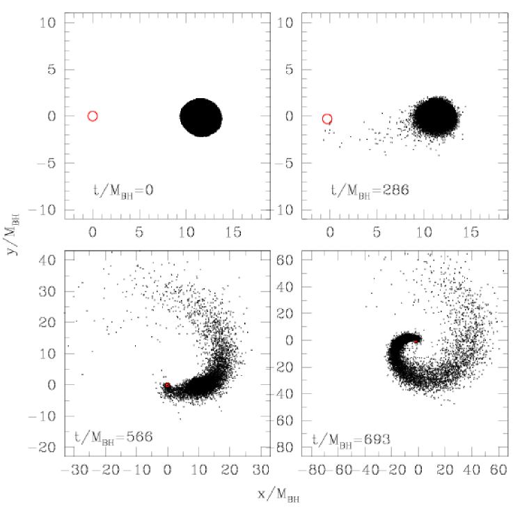
Figure 6: SPH particle configurations at times $t=0$, $286$, $566$, and $693$, projected into the orbital plane, for run A5 (for which the orbital period is $T=287~{}M_{\rm BH}$). These configurations correspond to the initial configuration, and after $1$, $2$, and $2.5$ full orbits, respectively. The BH is shown as a circle at a radius $r=0.5M_{\rm BH}$. We see that once mass transfer begins, the NS begins to expand, forming a low-density single-armed spiral pattern. Note that particles have different masses, and that those in the center of the NS are in most cases significantly more massive than those originally in the outer layers.

A similar pattern holds for all runs we performed with the same soft EOS, regardless of the binary separation. Due to the nature of the instability, all models we calculated led to the eventual tidal disruption of the NS, since there is no stabilizing mechanism to suppress mass loss once mass transfer begins, no matter how small the mass-transfer rate. It does take longer for the NS to be disrupted in configurations placed at a greater initial binary separation, however. In the bottom plot of Fig. 7, we show the evolution of the mass loss over time for all of the configurations using the soft NS EOS, defined as the total mass that can be found outside the innermost computational domain at any given time. We see that in all cases mass loss is an unstable process, occurring at a rate that grows extremely rapidly until the majority of its original mass is no longer bound to the NS. In the case started from the largest separation, slightly over half of the NS mass is accreted directly onto the BH or into orbits that lie within the ISCO, while half is lost outward to form the “spiral arm” pattern seen in Fig. 6. This pattern is to be expected, as the primary response of the NS to losing mass is expansion. The inner half of the NS is pushed inward toward the BH, while the outer half expands outward. For a synchronized configuration, we know that the average specific angular momentum of the NS is generally greater than the specific angular momentum near the center-of-mass of the NS, since $j\equiv\vec{v}\times\vec{r}\sim\Omega r^{2}$ is weighted more heavily by matter on the outside of the NS. In response to the expansion of the NS, we expect the orbit to tighten, which is confirmed by the numerical results. In Fig. 7, we show the binary separation over time for the runs with a soft NS EOS. We see that the onset of mass transfer leads to a rapid decrease in the binary separation, prompting the explosive mass loss. Only in the late stages does the remnant of the NS begin to move back outward, but by then tidal disruption is inevitable.

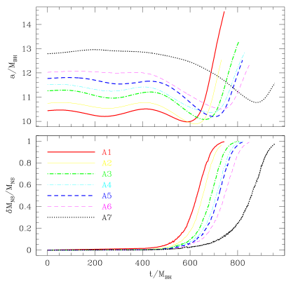
Figure 7: Binary separation (top panel) and total mass lost from the NS (bottom panel) as a function of time for all runs calculated using the soft NS EOS, runs A1-A7, which have $\Gamma=1.5$. The properties of the initial configurations, which differ only in their binary separation, are shown in Table 2. Here, particles are defined as “lost” when they lie outside the innermost computational domain around the NS. In all cases, mass loss never quenches once it begins, eventually leading to the complete disruption of the NS.

As the initial separation is decreased, the qualitative behavior of the system stays essentially the same, but more of the NS mass ends up being transferred inward toward the BH. In Fig. 8, we show the amount of mass lost inward (top panels) and outward (bottom panels) for all of the runs we performed with the soft EOS. For configurations near the stability limit, we find almost twice as much mass falls inward toward the BH as is expelled outward into the spiral arm. As these calculations were performed without radiation-reaction effects, we expect that including them would tip the balance of the mass transfer further toward mass accretion onto the BH, since the binary orbit will be driven by radiation to smaller separations than we find here.

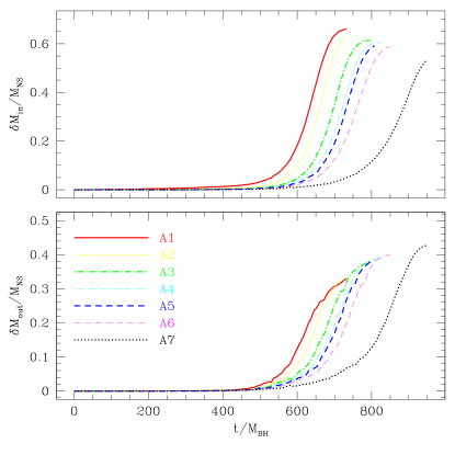
Figure 8: Total mass lost inward toward the BH (top panel) and outward away from the BH (bottom panel) as a function of time, for the runs shown in Fig. 7. In general, the smaller the initial separation, the more mass that falls inward toward the BH. For the runs started from a larger separation, much of the initial mass loss results from spurious numerical of low mass particles out of the Roche lobe, leading to nearly equal flows directed inward and outward. In contrast, the mass loss for the closer cases is in exactly the form expected for Roche-lobe overflow through the inner Lagrange point.

Unlike the situation found in NSNS binaries, for which $>99\%$ of the matter typically remains bound to the system, we find that a significant amount of matter is unbound from the system during all of our calculations with the soft EOS, representing in each run between $3-5\%$ of the original mass of the NS. This fraction is much larger than that typically found in relativistic calculations of synchronized binary NS systems Faber et al. (2004); Shibata et al. (2003), but roughly consistent with previous results from Newtonian BHNS calculations Lee and Kluźniak (1999b); Rosswog et al. (2004). However, we note that this fraction is almost certainly an overestimate, perhaps greatly so: irrotational configurations suppress the amount of mass that will become unbound (see, e.g., Faber and Rasio (2002) or FGR for a similar argument with respect to NSNS mergers) . The total angular momentum of an irrotational configuration is less than that of a synchronized configuration, and the decrease in specific angular momentum is largest at the outer edge of the NS. Thus, we expect that while some mass may still be unbound when the NS is initially irrotational, the amount may be significantly less.

V.2 BHNS mergers with a stiffer EOS: $\Gamma=2$

To study a configuration that would be predicted to undergo stable mass transfer in the classical conservative quasiequilibrium scenario, described in Sec. II.2, we model the NS with a stiffer, $\Gamma=2$ polytropic EOS, which has been used in numerous studies as a first approximation to a stiff NS EOS. We note that in Newtonian physics, this is the critical polytropic index for which an isolated NS has a radius independent of its mass. In relativistic gravity, self-gravity effects cause the NS radius to increase as the NS mass decreases.

V.2.1 Evolution without GW radiation-reaction

In Fig. 9 we show the binary separation (top panels) and NS mass fraction lost (bottom panels) as a function of time for runs B1-B4. We find three qualitatively different behaviors over time, which we will describe in turn. We note first that the tidal limit separation is not drastically different for this EOS compared to the softer EOS. Both cases show very good agreement with the classical Roche limit result, as we would expect.

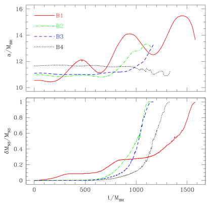
Figure 9: Binary separation (top panel) and total mass lost from the NS (bottom panel) as a function of time for the runs calculated using the stiff NS EOS without GW radiation-reaction, runs B1-B4, which have $\Gamma=2$. Conventions are as in Fig. 7. For run B1, we see periodic mass loss, as the NS gets kicked into an elliptical orbit, losing mass during every periastron passage. Runs B2 and B3 are similar to those with the softer EOS, as the NS gets disrupted during the first mass loss phase. Run B4 is essentially stable, only showing the long-term effects of numerical diffusion of particles.

Run B4 is completely stable for approximately three orbits. Eventually, the NS begins to lose a small amount of mass, which gives us an estimate for the length of time over which the code can reliably maintain an equilibrium configuration in the absence of relaxation ($t/T\sim 3$). We note from Fig. 10 that the mass loss from the NS is almost evenly divided between a component moving toward the BH and the component directed away, indicating that the mass loss is a numerical artifact caused by particles near the edge of the NS diffusing outside the Roche lobe over time.

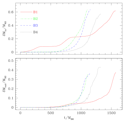
Figure 10: Total mass lost inward toward the BH (top panel) and outward away from the BH (bottom panel) as a function of time, for the runs shown in Fig. 9. Conventions are as in Fig. 8. Approximately $50\%$ more mass is lost inward for runs B2 and B3, started from near the stability limit, whereas for run B1, marked by an elliptical orbit and periodic mass transfer, nearly $4$ times much mass is lost toward the BH.

Runs B2 and B3 are started from a binary separation approximately equal to the mass-shedding limit. In both cases, the NS makes approximately one orbit after mass transfer begins without any appreciable change in the binary separation. By this point, approximately $10\%$ of the NS mass is stripped away, and the binary begins to move outward. As we saw in the case of the softer EOS, the mass loss is unstable and the mass-transfer rate grows rapidly. In both cases, the NS is tidally disrupted before the mass transfer halts. By the time the NS is disrupted, approximately $60\%$ of the original mass has fallen inward toward the BH, as we see from Fig. 10. Of the matter shed outward, approximately $0.075M_{\rm NS}$ is unbound from the system. This result fits in with the general picture derived from NSNS binaries, in which mass shedding outward is more efficient for stiffer EOS (see, e.g., Faber et al. (2001) and references therein).

The evolution of the NSs in runs B2 and B3 started from initial conditions differing only in their binary separations (run B3 starts from $0.5\%$ further out), which are nearly equal to the mass-shedding limit. We find that the closer the NS is when mass transfer begins, the more mass is lost inward toward the BH relative to that lost outward, until the NS expands to the point that it greatly overfills its Roche lobe and mass loss becomes more isotropic around the axis describing the NS velocity.

These observations go a great deal toward clarifying the evolution seen in run B1, the only case in which the mass transfer was periodic, rather than continuous. Here the initial configuration places the NS within the mass-shedding limit, as GW losses would be expected to do for physical BHNS systems. Indeed,runs B3a and B3b, described in Sec. V.2.2, which include the effects of radiation reaction, are driven to approximately this binary separation by GW radiation-reaction energy and angular momentum losses. When mass transfer begins, it occurs only toward the BH, which causes the NS to move outward. This expansion in the orbit, which happens with no outwardly directed stream to counter the outward acceleration, occurs sufficiently fast that the Roche-lobe expansion is enough to quench mass transfer. At this point, the NS is on a continuously expanding eccentric orbit ($e\sim 0.1$), whose apocenter lies outside the Roche limit and pericenter within it. As the NS crosses over the new mass-shedding limit, mass transfer begins again, pushing the NS onto an even wider eccentric orbit, similar to the pattern seen in Rosswog et al. (2004) for NS with a stiffer EOS.

This scenario is ostensibly similar to that proposed by Davies et al. (2005), but with one crucial difference. In both cases, mass transfer forces the NS onto a highly elliptical orbit. Here, however, mass transfer occurs during every periastron passage, whereas in their model the NS can be kicked into such a widely separated orbit that GW radiation-reaction must drive the NS back toward the mass-shedding point. We believe that the assumptions that go into the latter model lead to this unphysical result. In Davies et al. (2005), it is assumed that the NS loses a specified amount of mass during mass-transfer events but recovers half of its angular momentum during the next half orbital period. This can lead to a discontinuous evolution of the binary separation. Here, we see that once mass transfer ceases, the NS will follow a nearly unperturbed elliptical orbit, with essentially no change in its orbital angular momentum. Mass transfer must resume when the orbit crosses this same point as it approaches pericenter during the next passage.

V.2.2 Mergers including GW radiation-reaction

While evolution calculations lacking GW radiation-reaction terms can be useful for studying the processes that control the moment to moment dynamical evolution of the system, we know that the effects of radiation-reaction must play an important role in the secular dynamics of the system. Indeed, given the potentially unstable nature of mass loss, we expect the inwardly directed component of the NS velocity to be critical. Since the mass transfer leads not to an instantaneous change in the NS velocity, but rather in its acceleration, there will be a time period immediately after the onset of mass transfer during which the NS loses mass while falling further inward. All the while, the inner Lagrange point will move further within the NS, regardless as to how its radius adjusts on the dynamical timescale.

To model radiation-reaction, we add a damping force to the material, representing the lowest-order quadrupole contribution to the radiation reaction potential. Thus, we add to the RHS of Eq. (19) an acceleration term of the form

$$a_{i:reac}=N^{2}hu^{0}\partial_{i}\chi,$$ (70)

where $\chi$ is a quadrupole radiation-reaction potential (see Sec. 36.1 of Misner et al. (1973)), defined here as

$$\chi=\frac{1}{5}x^{k}x^{l}Q^{[5]}_{kl},$$ (71)

in terms of the fifth time derivative of the quadrupole moment,

$$Q_{kl}=STF\left[\int\rho_{\rm ADM}x_{k}x_{l}d^{3}x\right].$$ (72)

Here $\rho_{\rm ADM}$ is the quantity that can be integrated to give the matter contribution to the ADM mass $\rho_{\rm ADM}\equiv\psi^{5}E$, which appears in the field equation for $\psi$, Eq. (25). Following the argument found in Sec. IIIa of FGR, we evaluate the fifth time derivative of the quadrupole moment in terms of the expression for the first time derivative in the limit that it is dominated by terms representing orbital motion and not changes in the density with time (i.e., $d\rho_{\rm ADM}/dt$ is negligible),

$$(\dot{Q}_{1})_{kl}=STF\left[\int\rho_{\rm ADM}(x_{k}v_{l}+x_{l}v_{k})d^{3}x\right],$$ (73)

where “STF” means the symmetric trace-free component of the tensor. We then assume that further time derivatives result purely from the orbital motion, and approximate

$$Q^{[5]}_{kl}\approx 16\omega^{4}\dot{Q}_{kl},$$ (74)

where the angular velocity $\omega$ is taken as the ratio of the angular momentum to the moment of inertia,

$$\omega=\frac{\sum_{a}m_{a}(x_{a}(v_{y})_{a}-y_{a}(v_{x})_{a})}{\sum_{a}m_{a}(x_{a}^{2}+y_{a}^{2})}.$$ (75)

While the resulting radiation-reaction force will differ slightly from the true quadrupole expression found by taking the exact time derivatives, it is sufficiently accurate for our purposes here, generally within $10\%$. It is important to remember that the radiation-reaction force drives the binary inward on a secular timescale $t_{\rm GW}$, but plays almost no role once effects occurring on the much more rapid dynamical timescale become dominant.

To test how radiation-reaction effects change the scenario described above, we calculated two runs that included radiation-reaction terms. Both took as initial data the configuration used also for run B3, using the stiffer $\Gamma=2$ NS EOS, placed nearly at the stability limit. For run B3a, we added a radiation-reaction acceleration term described by Eq. (70); for run B3b, we doubled the magnitude of this force. The evolution of the former, run B3a, is shown in Fig 11. Mass transfer occurs in a well-defined stream for the first two orbital periods, until the expansion of the NS eventually drives the rapid tidal disruption of the NS.

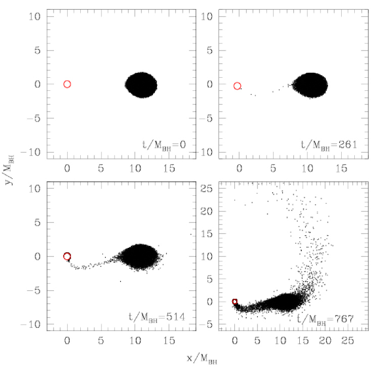
Figure 11: SPH particle configurations at times $t/M_{\rm BH}=0$, $261$, $514$, and $767$, projected into the orbital plane, for run B3a, which includes the dissipative effects of radiation-reaction (for this configuration, $T=265M_{\rm BH}$). In terms of the binary orbit, these correspond to the initial configuration and $1$, $2$, and $3$ full orbits, respectively. Conventions are as in Fig. 6. Here, we see that radiation-reaction initially drives only an inwardly directed mass-transfer stream onto the BH, until somewhere after $t/M_{\rm BH}=700$, when the expansion of the NS becomes unstable and tidal disruption occurs.

In Fig. 12, we show the evolution of the binary separation (top panels) and NS mass loss (bottom panels) for runs B3a and B3b. We find that the stronger the radiation-reaction losses, the greater the initial mass loss from the NS, since the first passage within the mass-shedding limit takes it closer to the BH. This in turn drives the NS back outward, quenching the mass loss temporarily until the next periastron passage, after which the NS tidally disrupts. From Fig. 13, we see that stronger radiation-reaction losses favors a larger amount of mass lost inward onto the BH (and thus less outward into a disk), as one would expect. Thus, we conclude that the inclusion of GW radiation-reaction terms have the effect of increasing the chance that some fraction of the original NS mass will remain bound after an initial phase of mass loss, since the NS rebounds more sharply outward than for cases in which radiation-reaction losses are ignored. Tidal disruption, while still seemingly inevitable, also occurs at a greater distance from the BH.

Figure 12: Binary separation (top panel) and total mass lost from the NS (bottom panel) as a function of time for the runs calculated using the stiff NS EOS and dissipative GW radiation-reaction effects, runs B3a and B3b, which have $\Gamma=2$. Conventions are as in Fig. 7. The only difference between the two runs is the magnitude of the radiation-reaction effects; we use the quadrupole order form in run B3a, and double its strength for run B3b. We find that doubling the radiative drag force forces the binary to a smaller separation, leading to a larger initial burst of mass loss and a more rapid increase in the binary separation. As a result, the system tidally disrupts slower than the case shown in run B3a.

Figure 13: Total mass lost inward toward the BH (top panel) and outward away from the BH (bottom panel) as a function of time, for the runs shown in Fig. 9. Conventions are as in Fig. 8. Initially, in run B3b with twice the physical GW radiation-reaction force applied, all mass lost in run B3b is directed inward. This leads to a rapid increase in the binary separation and slows the growth of the mass-transfer rate. In contrast, in run B3a, mass loss is more evenly balanced between inwardly and outwardly directed flows, and the NS disrupts more quickly.

In the bottom panel of Fig. 14, we show the gravity wave signal produced in run B3a, in both polarizations. The two components are defined by the familiar relations

$$D_{o}h_{+} = \ddot{Q}_{xx}-\ddot{Q}_{yy},$$ (76)

$$D_{o}h_{\times} = 2\ddot{Q}_{xy},$$ (77)

where $D_{o}$ is the distance from the observer to the binary. The corresponding angular frequency of the GW signal, approximately equal to twice the orbital angular frequency, is shown in the top panel of the figure. Prior to disruption, the GW waveform takes the classic point-mass form, with a steadily but extremely slowly increasing amplitude and frequency (relativistic and finite-size affects cause minor deviations from the point-mass form; see Faber et al. (2002) for a discussion). Once the mass transfer begins, however, the frequency reaches a maximum and begins to decrease quickly, as does the amplitude. In general, if the NS does transfer sufficient mass to survive the initial infall, we expect this decrease in frequency and amplitude until the signal can no longer be reliably observed. Should the orbit be elliptical, as we found for run B1, this will show up in the GW waveform as well.

As matter accretes onto the BH, it will excite quasi-normal ringing modes that could in theory be visible in the gravitational wave signal. Unfortunately, our numerical approach limits our ability to determine the gravitational wave signal we expect from these modes. Indeed, such a calculation would require a dynamical treatment of the spacetime very near the BH, whereas in our calculation, the key physics for ringdown occurs in the asymptotic region located outside our computational domain, where the BH remains stationary. To evaluate quasi-normal mode ringing, it will be necessary to relax the CF approximation, in which no gravitational radiation is generated, and to evolve the fields everywhere. Additionally, the use of a lapse function that penetrates the horizon will be crucial for studying the problem self-consistently. We plan to study these issues in future work.

Figure 14: Gravity wave emission angular frequency (top panel) and waveform in both polarizations, $h_{+}$ (solid curve) and $h_{\times}$ (dashed curve), defined by Eqs. (76) and (77), for the merger calculated in run B3b. Initially, we see conclusion of the standard “chirp” signal, in which the binary separation decreases while the GW amplitude and frequency increases, all of which happens extremely gradually on the secular GW timescale. This lasts until the onset of mass transfer, at which point we encounter a much more rapid “reverse chirp”, as the GW amplitude and frequency rapidly decrease while the NS is tidally disrupted.

VI Summary and Discussion

We have performed relativistic calculations of BHNS mergers in CF gravitation, in the limit that the BH is much more massive than the NS. These calculations mark the first time that a relativistic treatment has been applied both to the self-gravity of the NS as well as the BH spacetime.

For systems studied here in which the onset of tidal disruption occurs outside the ISCO, previously proposed analytical models do not properly describe all the complex tidal phenomena that pertain to the evolution. In all the runs we calculated, mass transfer plays a leading role in determining the dynamics of the system. In general, mass transfer in a stream directed toward the BH causes the orbital separation to increase, in many cases quite dramatically. Mass transfer also causes the NS radius to expand on the dynamical timescale, with relativistic self-gravity effects leading to a more rapid expansion than is seen in Newtonian gravity for a given NS EOS. As a result, mass transfer is significantly more unstable in relativistic gravity. We conclude immediately that previous models of mass transfer in compact object binaries that assume the orbit remains quasi-circular Clark and Eardley (1977); Portegies Zwart (1998) are not applicable here. Furthermore, the model put forward in Davies et al. (2005) also seems to be insufficient, in that the orbital parameters evolve discontinuously from one orbit to the next (as a result of angular momentum being added to the NS while its mass is held fixed). We find instead that if some remnant of the NS survives the initial burst of mass loss, it can end up on an elliptical orbit that takes it back outside its mass-shedding separation. During every successive periastron passage, however, more mass will be lost, eventually leading to the complete disruption of the NS.

As the NS expands during mass loss, it eventually loses mass outward as well as inward, so long as the plunge does not take it too far within the ISCO, leading to a prompt plunge onto the BH. While the majority of matter released through the outer Lagrange point remains bound to the BH in the former case, a significant fraction is ejected with sufficient velocity to become unbound from the system completely, approximately $5-7\%$ for the $\Gamma=2$ EOS we considered. This mass loss also limits the radial expansion of the orbit, and as a result we find in many of our calculations that mass transfer is never quenched once it begins. Even though the NS moves outward, it persists in configurations for which the Roche lobe lies within the star, and mass loss continues until the NS is completely disrupted.

We plan to improve our simulations and relax several approximations in the near future. In particular we plan to adopt the astrophysically more realistic irrotational initial configuration of TBFS instead of the corotating configurations used here. Relativistic NSNS Faber et al. (2004); Shibata and Uryū (2000) and Newtonian BHNS Rosswog et al. (2004) calculations have shown that for these cases the amount of matter ejected from the binary system is expected to be significantly smaller, since the material on the outer edge of the NS has significantly less specific angular momentum. Thus, while we expect that BHNS mergers will expel more material than in the case of NSNSs, in which the binary components are more comparable in mass, we would assume that the ejected fractions found here are overestimates.

Calculating mergers using irrotational NSs should also increase the probability that escaping matter forms an accretion disk around the BH, even if that disk is short-lived (see, e.g., Rosswog (2005b)). We typically found in our calculations here that most of the matter transferred toward the BH ends up accreting onto it directly, since the specific angular momentum is not sufficient to create a disk. Even though an irrotational NS has less total angular momentum than a corotating one, the matter on the inner edge has a higher specific angular momentum, and is more likely to orbit around the BH rather than infall directly. In addition, prompt accretion of matter may also be inhibited slightly by a moving BH orbiting the binary center of mass, whereas in our assumption of an extreme mass ratio, the BH position is fixed.

In our future work, we will test out how shock heating in the accretion disk affects its evolution, and determine if there are cases in which feedback onto the NS will affect its future evolution as well. By including a relativistic artificial viscosity treatment, we will follow the thermodynamic evolution of the disk, as well as that of the NS and any outward mass loss. Of course, to investigate BHNS mergers fully and accurately, we will ultimately have to abandon the assumptions underlying the CF metric as well. While our description of an isolated Schwarzschild BH is exact, the BH lapse goes to zero just outside the event horizon. This causes matter to “pile up” around the BH, since the proper time ceases to advance in this region. While this poses no difficulty for determining the fate of the material, which will clearly be accreted, it does act as a computationally challenging ridge of growing mass concentration as material is transferred continuously toward the BH.

These calculations adopted “undercompact” NSs because we are interested in systems that disrupt outside the ISCO while restricting our attention to the case of extreme mass ratios. By performing dynamical evolutions using more compact configurations, we will investigate the transition to the opposite case, in which plunge begins while the NS is still completely bound. Based upon our results, we expect that that in some cases, the mass-transfer rate may prove sufficient to kick the core of the NS back out to a wider, highly elliptical orbit. The phase space for which this will occur, in terms of the NS EOS and binary mass ratio, remains poorly understood, and may not conform to simple analytic estimates, which have difficulty describing the unstable processes that characterize the merger. In Rosswog et al. (2004), it was found for a quasi-Newtonian potential that for a mass ratio $q=0.1$, a NS described by a $\Gamma=2$ EOS was disrupted during the initial passage, whereas one with a $\Gamma=3$ EOS led to a punctuated mass-transfer scenario similar to the one we describe for run B1 above in Sec. V.2.2. Probing the assumed forms of the NS EOS that lead to complete disruption versus survival of a remnant NS core may prove to be a crucial diagnostic tool for determining the true physical NS EOS.

In many prior works, it has been assumed that so long as $a_{ISCO}<a_{Roche}$, the NS will necessarily be tidally disrupted, with some of its mass deposited into a disk around the BH. According to Miller (2005), this may not be true. Instead, the plunge may start well outside of the ISCO, since, based on the properties of quasiequilibrium models, the inspiral time scale may approach the orbital time scale already well outside of the ISCO (so that the transition through the ISCO is nearly dynamical rather than adiabatic). It is unclear exactly what role the spin of the BH will play in this process, though it appears that a prompt merger is more likely for a Schwarzschild BH than a spinning Kerr BH Rasio et al. (2005), where the latter case is favored by binary evolution calculations Podsiadlowski et al. (2003); O’Shaughnessy et al. (2005).

Two different factors can mitigate a prompt merger, however, and will need to be investigated numerically in more detail. First, the onset of a “plunge” also marks the point at which we assume the quasi-equilibrium formulation to break down. From that point onward, the NS will no longer follow the trajectory predicted by quasiequilibrium results, and may therefore not plunge as fast as quasiequilibrium models would predict (in fact, these predictions provide completely unphysical overestimates of the infall velocity at the ISCO itself). Perhaps more importantly, there is no guarantee that a plunge phase will lead to the entire NS being swallowed by the BH Rosswog (2005b). Angular momentum can be transferred outward within the NS on something approximating the dynamical timescale, and it is possible that some fraction of the mass, perhaps a significant fraction, will survive the initial plunge phase. Using the techniques developed here, and initial configurations taken from TBFS, we will study how varying the NS spin and compaction affect the final fate of the NS.

It will be necessary to perform relativistic merger calculations in full generality, in order to drop the assumption that the binary mass ratio is extreme. We are currently constructing such quasiequilibrium data, which will then serve as initial data for dynamical simulations Taniguchi et al. (2005b). We expect that these dynamical simulations will be plagued by the same difficulties encountered in dynamical simulations of BHBH binaries, and therefore anticipate that this will be a very challenging project.

Until that point, however, a great deal can be accomplished. First and foremost would be to identify the boundaries in phase space that separate qualitatively different phenomena that can occur during a BHNS merger. The most obvious categories would be prompt merger, prompt tidal disruption leading to an accretion disk, or a period of periodic mass-transfer bursts, if the latter does occur at all. The former distinction should prove useful for understanding any potential X-ray/gamma-ray emission from these systems, and aid in our understanding of short gamma-ray bursts like the recently observed GRB 050509b Bloom et al. (2005); Gehrels et al. (2005), GRB 050709 Covino et al. (2005); Fox et al. (2005), GRB 050724Berger et al. (2005), and GRB 050813Retter et al. (2005).

Appendix A Mass transfer in the viscous regime

Below, we derive a formalism that can be used to describe conservative quasiequilibrium mass transfer, for those cases where the viscosity is high, and the binary orbit remains circular during the mass-transfer process. For typical (high-mass) NSs, this regime does not apply (Bildsten and Cutler (1992); Kochanek (1992); see also Fig. 1 above), but can apply to low-mass NSs, WDs, and main sequence stars orbiting BHs. We nevertheless refer to the star as a NS below.

A.1 Newtonian polytropes

In Newtonian physics, the mass-radius relationship is given as a function of the polytropic index $n$ by

$$R_{\rm NS}\propto M_{\rm NS}^{(1-n)/(3-n)}.$$ (78)

For a given value of the parameter $\kappa$ in $P=\kappa\rho_{0}^{(1+1/n)}$, the familiar result is that NSs with $n=1$ have a uniform radius independent of their mass. NSs with $n<1$ have radii which decrease as the mass decreases, whereas those with $n>1$ increase in size as they lose mass. We see that if the NS loses mass at a rate $\dot{m}\equiv-\dot{M}_{\rm NS}$ (implying $\dot{m}>0$ for the case of interest), the change in the radius is given by

$$\frac{\dot{R}_{\rm NS}}{R_{\rm NS}}=\frac{n-1}{3-n}\frac{\dot{m}}{M_{\rm NS}}.$$ (79)

Once mass transfer begins, the NS will shed mass, and in doing so, lose both energy and angular momentum. This will affect the binary orbit, in a way which depends on both the magnitude and fate of the angular momentum of the ejected material.

For conservative mass transfer, the orbital angular momentum $J$ and the total binary mass $M_{T}\equiv M_{\rm NS}+M_{\rm BH}=(1+q)M_{\rm NS}/q$ are conserved globally, as mass is transferred from the NS to the BH. We assume that the orbit remains circular. Since $q=M_{\rm NS}/(M_{T}-M_{\rm NS})$, we see that

$$\frac{\dot{q}}{q}=-(1+q)\frac{\dot{m}}{M_{\rm NS}}.$$ (80)

From the angular momentum of a circular orbit,

$$J=M_{\rm NS}M_{\rm BH}\sqrt{\frac{Ga}{M_{T}}},$$ (81)

we find that

$$a = \frac{M_{T}J^{2}}{G}\left[M_{\rm NS}(M_{T}-M_{\rm NS})\right]^{-2}$$ (82)

$$= \frac{J^{2}}{G}M_{\rm NS}^{-3}q(1+q),$$

$$\dot{a}/a = 2(1-q)\frac{\dot{m}}{M_{\rm NS}}.$$ (83)

The Roche-lobe radius $R_{r}$ changes during the process as well. Taking the logarithmic time derivative of Eq. (2) and combining with Eq. (83), we find

$$\frac{\dot{R}_{r}}{R_{r}} = \frac{\dot{a}}{a}+\frac{\dot{q}}{3q(1+q)}$$ (84)

$$= \frac{\dot{a}}{a}-\frac{\dot{m}}{3M_{\rm NS}}=\frac{5-6q}{3}\frac{\dot{m}}{M_{\rm NS}}.$$

Combining this final expression with Eq. (79), we see that mass transfer will be unstable if $\dot{R}_{\rm NS}/R_{\rm NS}>\dot{R}_{r}/R_{r}$, or equivalently,

$$n > \frac{9-9q}{4-3q},$$ (85)

$$q > \frac{9-4n}{9-3n},$$ (86)

or in terms of the adiabatic index $\Gamma\equiv 1+1/n$, mass transfer is unstable if

$$\Gamma < \frac{13-12q}{9-9q},$$ (87)

$$q > \frac{9\Gamma-13}{9\Gamma-12}.$$ (88)

In particular, the critical mass ratio for unstable mass transfer for some polytropic indices commonly used in numerical calculations are

$$n=1/2~{}(\Gamma=3) : q>14/15,$$ (89)

$$n=1~{}(\Gamma=2) : q>5/6,$$ (90)

$$n=3/2~{}(\Gamma=5/3) : q>2/3.$$ (91)

As a general rule, for polytropic indices $n<3/2$, mass transfer is stable only for systems with components of similar mass. For $n>3/2$, the critical mass ratio drops quickly, down to the limiting case $n=9/4$, the softest polytropic EOS for which stable mass transfer can ever occur, at which point $q=0$.

A.2 Relativistic polytropes

Relativistic polytropes are not self-similar for a fixed value of the polytropic index; as the mass decreases, non-linear gravitational effects become weaker, and the star’s scale-free density profile grows in size. It is straightforward to incorporate this into our discussion of mass transfer. We recast the mass-radius relationship in the form

$$R_{\rm NS}\equiv\xi M_{\rm NS}^{(1-n)/(3-n)}f({\cal C}),$$ (92)

where $\xi$ sets the physical scale of the mass-radius relation, ${\cal C}\equiv M/R$ is the compactness of a spherical star, and $f({\cal C})$ accounts for the relativistic corrections to the mass-radius relation. Since relativistic corrections effectively increase the strength of gravity, $f({\cal C})$ must be a monotonically decreasing function of compactness. As ${\cal C}\rightarrow 0$, $\xi$ approaches the proper Newtonian value, $\xi=\xi_{N}$, and $f(0)\rightarrow 1$. Taking a logarithmic derivative of Eq. (92) shows us that

$$\frac{\dot{R}_{\rm NS}}{R_{\rm NS}}=\frac{\dot{f}}{f}+\frac{n-1}{3-n}\frac{\dot{m}}{M_{\rm NS}}.$$ (93)

But we know

$$\frac{\dot{f}}{f}=\frac{1}{f}\frac{\partial f}{\partial{\cal C}}\dot{{\cal C}} = \frac{1}{f}\frac{\partial f}{\partial{\cal C}}\left[\frac{\dot{M}_{\rm NS}}{R_{\rm NS}}-\frac{M\dot{R}_{\rm NS}}{R_{\rm NS}^{2}}\right]$$ (94)

$$= -\frac{{\cal C}}{f}\frac{\partial f}{\partial{\cal C}}\left[\frac{\dot{m}}{M_{\rm NS}}+\frac{\dot{R}_{\rm NS}}{R_{\rm NS}}\right],$$

so we conclude that

$$\frac{\dot{R}_{\rm NS}}{R_{\rm NS}}=\left[\frac{n-1}{3-n}-\frac{2}{3-n}\frac{{\cal C}}{f}\frac{\partial f}{\partial{\cal C}}\left(1+\frac{{\cal C}}{f}\frac{\partial f}{\partial{\cal C}}\right)^{-1}\right]\frac{\dot{m}}{M_{\rm NS}}.$$ (95)

From Eq. (85), we see that the critical mass ratio for instability becomes

$$q_{c}=\frac{9-4n}{9-3n}+\frac{1}{3-n}\frac{{\cal C}}{f}\frac{\partial f}{\partial{\cal C}}\left(1+\frac{{\cal C}}{f}\frac{\partial f}{\partial{\cal C}}\right)^{-1},$$ (96)

where the second term is always negative, indicating that more compact configurations are more unstable against mass transfer.

In Figure 15, we show the critical compactness values separating stable and unstable mass transfer for relativistic polytropes, as a function of the binary mass ratio and the polytropic (bottom panels) and adiabatic (top panels) indices. As a general rule, as the compactness of the NS increases, mass transfer is more likely to be unstable. The Newtonian curves (${\cal C}=0$) have an analytic form given by Eqs. (85) and (87). Also shown are the two models we evolve dynamically in this paper, both with ${\cal C}=0.042$. The case with $n=1(\Gamma=2)$, shown as a triangle, would be expected to demonstrate stable mass transfer in the highly viscous regime, but as we show in Sec. V.2, the true situation is nowhere near this simple for typical NSs. The case with $n=2(\Gamma=1.5)$, shown as a square, is expected to lead to unstable mass transfer.

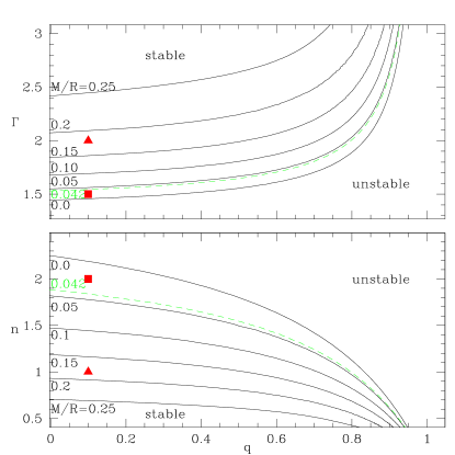
Figure 15: Critical compactness for determining the stability of mass transfer from a relativistic polytropic NS companion as a function of the binary mass ratio, defined in terms of the polytropic index $n$ (bottom), or the adiabatic index $\Gamma\equiv 1+1/n$. Mass transfer is unstable to the right of the curve, stable to the left. The square and triangle represent the positions of the two models we are evolving dynamically.

Representing the same results against compactness, rather than mass ratio, shows how little parameter space is available for unstable mass transfer in the viscous limit. In Figure 16, we show the critical binary mass ratio for stable or unstable mass transfer as a function of the NS compactness and polytropic (bottom) or adiabatic (top) index. We see that for a given compactness, there is a rather limited range of polytropic indices which can produce unstable mass transfer. The heavy lines show the maximum possible compactness allowed for a given polytropic EOS; no model to the right of those curves can be constructed. The models that we evolve dynamically are shown as well. As noted in Sec. V.2, many models expected to undergo stable mass transfer in the viscous limit are extremely unstable during mass transfer when viscosity is not a dominant driver of the evolution Bildsten and Cutler (1992); Kochanek (1992), so the true parameter space for instability is actually much larger for typical NSs than analytic models would otherwise predict.

Figure 16: Critical mass ratio for determining the stability of mass transfer from a relativistic polytropic NS companion as a function of the NS compactness, defined in terms of the polytropic index $n$ (bottom), or the adiabatic index $\Gamma\equiv 1+1/n$. Mass transfer is unstable to the right of the curve, stable to the left. The heavy solid lines depict the maximum possible compaction for a given polytropic EOS. The square and triangle represent the positions of the two models we are evolving dynamically.

A.3 Time evolution

We describe here a crude treatment of the dynamics of mass transfer in the presence of gravitational radiation-reaction losses, using a number of simplifying assumptions. Most important among these will be treating the problem in the quasi-equilibrium regime.

We will study only conservative mass transfer, in the highly viscous limit. The evolution of the binary separation can be derived from the expression for the total angular momentum for a circular orbit, Eq. (81). Making no assumptions about the evolution of the system angular momentum, we find

$$\frac{\dot{J}}{J}=\frac{\dot{M_{\rm NS}}}{M_{\rm NS}}+\frac{\dot{M_{\rm BH}}}{M_{\rm BH}}+\frac{\dot{a}}{2a}=(q-1)\frac{\dot{m}}{M_{\rm NS}}+\frac{\dot{a}}{2a}.$$ (97)

Setting the RHS equal to zero gives the standard expression for conservative mass transfer, Eq. (83). For the case of a relativistic binary, we know angular momentum will not be conserved. Instead, angular momentum is radiated away from the system in gravitational waves. As we are assuming circular orbits, we will make use of the standard angular momentum loss rate,

$$\frac{\dot{J}}{J}=-\frac{32}{5}\frac{M_{\rm NS}M_{\rm BH}M_{T}}{a^{4}}.$$ (98)

From our two angular momentum relations, we can derive a relation linking the mass loss rate to the change in binary separation, and determine the time-averaged mass loss rate. To do so, we will make a very simple assumption: that mass loss takes place at the location where we predict Roche-lobe overflow to occur.

Solving Eq. (84) for the binary separation and assuming $R_{r}=R_{\rm NS}$, we can insert Eq. (95) and find

$$\frac{\dot{a}}{a}\!\! = \frac{2n}{9-3n}\frac{\dot{m}}{M_{\rm NS}}+\frac{\dot{f}}{f}$$ (99)

$$= \!\!\!\!\frac{2}{3-n}\left[\frac{n}{3}-\frac{{\cal C}}{f}\frac{\partial f}{\partial{\cal C}}\left(1+\frac{{\cal C}}{f}\frac{\partial f}{\partial{\cal C}}\right)^{-1}\right]\frac{\dot{m}}{M_{\rm NS}}.$$

Plugging this result into Eq. (97), we find

$$\frac{\dot{J}}{J}=-\left[\frac{9-4n}{9-3n}-q+\frac{1}{3-n}\frac{{\cal C}}{f}\frac{\partial f}{\partial{\cal C}}\left(1+\frac{{\cal C}}{f}\frac{\partial f}{\partial{\cal C}}\right)^{-1}\right]\frac{\dot{m}}{M_{\rm NS}}.$$ (100)

Re-expressing the radiation-reaction angular momentum loss rate, Eq. (98), for a binary located at the Roche-lobe overflow point, we find

$$\frac{\dot{J}}{J}\!\! = -\frac{32}{5}\frac{M_{\rm NS}M_{\rm BH}M_{T}}{\left(0.46R_{\rm NS}M^{1/3}m_{1}^{-1/3}\right)^{4}}$$ (101)

$$= \!\!\!-143\xi^{-4}\!f({\cal C})^{-4}(\!M_{T}\!-M_{\rm NS})\!M_{T}^{-1/3}\!M_{\rm NS}^{\frac{9+5n}{9-3n}}.$$

We are now in a position to analyze the mass-transfer process from its onset until the final fate of the binary. To do so, we will make a few simplifying assumptions. First, we assume the NS is much less massive than the BH, such that $M_{\rm BH}\sim M_{T}$ and $q\ll 1$. Also, we will ignore the relativistic changes to the Newtonian power-law mass-radius relation, which has the effect of setting $f=1$ uniformly (and thus $\partial f/\partial{\cal C}=0$). In general, relativistic polytropes expand more than their Newtonian analogues during mass loss, which increases the amount of orbital expansion seen for a given amount of mass loss. This statement would imply that a given amount of mass loss leads to a greater loss of angular momentum, or conversely, that for a fixed angular momentum loss rate we would see a slight suppression of the mass loss rate. Under these assumptions, we find

$$\frac{\dot{m}}{M_{\rm NS}} = 143\xi^{-4}M_{T}^{2/3}\frac{9-3n}{9-4n}M_{\rm NS}^{\frac{9+5n}{9-3n}}$$ (102)

$$= \frac{9-3n}{9-4n}\left(\frac{M_{\rm NS}}{M_{\rm NS}(0)}\right)^{\frac{9+5n}{9-3n}}\frac{1}{2t_{GW0}},$$

where we define $t_{GW0}$ as the infall timescale when the NS first reaches the onset of mass transfer, as defined by Eq. (5), and where $M_{\rm NS}(0)$ is the NS mass at this time. This equation has the solution

$$\frac{M_{\rm NS}(t)}{M_{\rm NS}(0)}=\left(1.0+\frac{9+5n}{9-4n}\frac{t}{2t_{\rm GW0}}\right)^{-\frac{9-3n}{9+5n}},$$ (103)

with asymptotic behavior

$$M_{\rm NS}(t) \propto t^{-\frac{9-3n}{9+5n}},$$ (104)

$$\dot{m} \propto t^{-\frac{18+2n}{9+5n}}.$$ (105)

Considering some familiar polytropic EOS, we find:

$$n=1.5~{}(\Gamma\!=5/3) : \!\!M\propto t^{-3/11};\dot{m}\propto t^{-14/11},$$ (106)

$$n=1.0~{}(\Gamma=2) : \!\!M\propto t^{-3/7};\dot{m}\propto t^{-10/7},$$ (107)

$$n=0.5~{}(\Gamma=3) : \!\!M\propto t^{-15/23};\dot{m}\propto t^{-38/23},$$ (108)

$$n=0~{}(\Gamma\rightarrow\infty) : \!\!M\propto t^{-1};\dot{m}\propto t^{-2}.$$ (109)

Eq. (106) recovers the special value found by Portegies Zwart (1998), in the limit $q\ll 1$. We note that the typical rate found here satisfies $\dot{M}_{\rm NS}\sim M_{\rm NS}/t_{GW0}$ [cf., Eq. (102)], while our dynamical simulations for cases in which viscosity is not important show $\dot{M}_{\rm NS}\gg M_{\rm NS}/t_{GW0}$.

Appendix B Symmetries

When constructing quasi-equilibrium configurations in either Newtonian or relativistic gravity, it is important to take note of the various symmetries present in the relevant equations. These symmetries can either be enforced numerically, to save computational resources, or be used as a check to make sure that a numerical code is producing physically valid results.

For quasi-equilibrium binary BHNS systems, virtually all gravitational formalisms will produce a configuration that is equatorially symmetric so long as the NS spin axes are parallel to the orbital angular momentum axis, regardless of whether the NS is corotating, counterrotating, or irrotational. If we fix the z-axis to be parallel to the various angular momenta mentioned above, we find that the transformation $z\rightarrow-z$, with a corresponding reflection for all vector and tensor quantities, leaves the hydrostatic equations and the metric invariant, and is compatible with the velocity field of the initial configuration as well. For quasi-equilibrium configurations evaluated using full GR in the Kerr-Schild metric, this is the only symmetry plane of note present in the initial data. In our calculations, this symmetry is enforced at the code level: each SPH particle is treated as if it were a pair of particles, each of half the total mass, with one copy lying above the equatorial plane and one below. All spectral decompositions include this symmetry as well, setting to zero all spherical harmonics that are incompatible with a fully symmetric description.

We show here that there is an additional symmetry plane for the case of equilibrium BHNS binaries in conformally flat gravity, because the formalism is time-symmetric. Directions are defined such that the axis of separation between the BH and NS lies along the x-axis, and the orbital angular momentum points in the z-direction. Thus, the y-direction represents the direction of motion for each object. Reversing the time direction requires us to perform two operations in order to maintain invariance. First, we must invert all vector quantities, most notably the velocity and the shift vector. Second, we must perform an inversion in the y-direction, to account for the inversion of our angular coordinate $\phi\rightarrow-\phi$. We find the following relations are compatible with the initial velocity field, and leave our hydrostatic equations invariant:

$${\rm Scalars} : f(x,y,z,t)=f(x,-y,z,-t),$$ (110)

$${\rm Vectors} : [v^{x},v^{y},v^{z}](x,y,z,t)=$$ (111)

$$~{}~{}~{}~{}-[v^{x},-v^{y},v^{z}](x,-y,z,-t).$$

Evaluating the expressions above at $t=0$ yields the symmetries in the y-direction for our initial data. This symmetry can be extended to tensor quantities as well: two index tensor elements satisfy the relation $T_{ij}(x,-y,z)=(-1)^{1+N_{y}}T_{ij}(x,y,z)$, where $N_{y}$ is the number of “y” indices present for a given element. The additional factor of $-1$ is necessary to describe the inversion properties under time symmetry. Equatorial symmetry can be described in the same language, $T_{ijk...}(x,y,-z)=(-1)^{N_{z}}T_{ijk...}(x,y,z)$.

It is straightforward to check that these symmetries are compatible with all equations governing the construction of quasi-equilibrium NS binaries in CF gravity. To do so, we note that any tensorial operation on fields satisfying these symmetries will maintain these symmetries, including gradients and inner products.

First, we note that the matter sources in the equations for the conformal factor and lapse function, Eqs. (25) and (26), $E$, $P$, and $S$, as scalars, are symmetric in both $y$ and $z$. The same pattern follows for scalar densities and quantities like $u^{0}$. As an immediate consequence, the lapse and conformal factor share the same symmetries, since the only other source terms involve $K_{ij}K^{ij}$, itself a scalar.

The equilibrium velocity field is $\vec{v}=\vec{\Omega}\times\vec{r}=\allowbreak[-\Omega y,\Omega x,0]$, which satisfies

$$[v^{x},v^{y},v^{z}](x,-y,z)=-[v^{x},-v^{y},v^{z}](x,y,z).$$ (112)

Equatorial symmetry is satisfied trivially. In the CF case, the BH component of the shift vector is zero, and also satisfies the symmetry relations trivially. Since the shift equation, Eq. (24) depends only on the velocity field and other tensors, we can extend the symmetry to describe all quantities present in the equation. This statement cannot be made for the Kerr-Schild metric, and serves as the simplest example of how time-symmetry fails. For the Kerr-Schild case,

$$\beta^{i}_{\rm BH-KS} \propto x^{i}\rightarrow$$ (113)

$$\!\!\!\!\!\!\!\!\!\!\!\!\!\!\!\!\!\!\!\!\!\!\!\=[\beta^{x},-\beta^{y},\beta^{z}](x,y,z).$$

Thus, the BH contribution to the shift satisfies a different symmetry relation than the initial velocity field, and there is no global symmetry present. The physical reasons underlying this fact are discussed in more detail in Appendix E of Yo et al. (2004b).

Appendix C Preserving Stationary Equilibrium During CF Evolution

We show here that the CF evolution equations maintain strict stationary equilibrium for initial data satisfying both the thin-sandwich equations and the integrated Euler equation. That is, if we have an initially uniformly rotating matter configuration that satisfies the condition $h/u^{0}=C$, where $C$ is constant throughout space at $t=0$, and if the gravitational field satisfies the CTS equations, Eqs. (24), (25), and (26), the time derivatives of all quantities go to zero. Note that under these assumptions, this statement applies to both Eulerian and Lagrangian time derivatives, related by the expression $d/dt=\partial/\partial t+v^{j}\partial/\partial x^{j}$ since the difference term goes to zero when $v^{j}=0$, which applies in the corotating frame.

First, we note that the continuity equation, Eq. (15), and energy equation, Eq. (22), are trivially conserved when $v^{i}=0$, implying that $\rho_{*}$ and $e_{*}$ are conserved automatically.

The only evolution equation that requires a more thorough look is the Euler equation, Eq. (19), which we re-express for convenience in the equivalent form

$$\frac{d\tilde{u}_{i}}{dt}=-\frac{\partial_{i}P}{\rho_{*}u^{0}}-\alpha hu^{0}\partial_{i}\alpha+\tilde{u}_{j}\partial_{i}\beta^{j}+\frac{2\tilde{u}_{k}\tilde{u}_{k}}{hu^{0}\psi^{5}}\partial_{i}\psi.$$ (114)

We can show that the RHS of this expression is zero by starting from the integrated Euler equation, which implies that

$$\frac{\partial_{i}h}{u^{0}}-\frac{h\partial_{i}u^{0}}{(u^{0})^{2}}=0,$$ (115)

From the relativistic Gibbs-Duhem relation, we know that Gourgoulhon et al. (2001)

$$\frac{\partial_{i}h}{u^{0}}=\frac{\partial_{i}P}{\rho_{0}u^{0}}.$$ (116)

The gradient of $u^{0}$ is determined from the normalization $u_{a}u^{a}=u_{0}u^{0}=-1$, where we make use of the fact that $u^{i}=0$. From this, we conclude

$$u^{0}=(\alpha^{2}-\psi^{4}\delta_{ij}\beta^{i}\beta^{j})^{-1/2},$$ (117)

and differentiating,

$$\partial_{i}u^{0}=-(u^{0})^{3}(\alpha\partial_{i}\alpha-\psi^{4}\delta_{jk}\beta^{j}\partial_{i}\beta^{k}-2\psi^{3}\delta_{jk}\beta^{j}\beta^{k}\partial_{i}\psi).$$ (118)

Inserting the expression $u_{i}=g_{0i}u^{0}=-\psi^{4}u^{0}\delta_{ij}\beta^{j}$ for a configuration with $u^{i}=0$, we see that

$$\frac{h\partial_{i}u^{0}}{(u^{0})^{2}}=-\left(\alpha hu^{0}\partial_{i}\alpha+\tilde{u}_{k}\partial_{i}\beta^{k}-\frac{2\tilde{u}_{k}\tilde{u}_{k}}{hu^{0}\psi^{5}}\partial_{i}\psi\right),$$ (119)

and combining terms,

$$0 = \partial_{i}\left(\frac{h}{u^{0}}\right)=\frac{\partial_{i}h}{u^{0}}-\frac{h\partial_{i}u^{0}}{(u^{0})^{2}}$$ (120)

$$= \frac{\partial_{i}P}{\rho_{0}u^{0}}+\left(\alpha hu^{0}\partial_{i}\alpha+\tilde{u}_{k}\partial_{i}\beta^{k}-\frac{2\tilde{u}_{k}\tilde{u}_{k}}{hu^{0}\psi^{5}}\partial_{i}\psi\right)$$

$$= -\frac{d\tilde{u}_{i}}{dt}=0.$$

Thus, the RHS of the Euler equation, Eq. (19), is zero under these assumptions, and $\tilde{u}_{i}$ is also invariant.

We now consider the field equations for the CTS initial data. The fields are described by a set of linked elliptic equations, Eqs. (24), (25), and (26), whose source terms involve the fields themselves, as well as three quantities:

$$E = (\alpha u^{0})^{2}[\frac{\Gamma P}{\Gamma-1}+\rho_{0}]-P,$$ (121)

$$U^{i} = \frac{\delta^{ij}u_{j}}{\psi^{4}\gamma_{n}(1+\Gamma\epsilon)},$$ (122)

$$S = 3P+\psi^{4}(E+P)\delta_{ij}U^{i}U^{j},$$ (123)

where $\rho_{0}$, $\epsilon$, and $P$ are the standard relativistic mass density, internal energy density, and pressure, respectively. The Lorentz factor $\gamma_{n}\equiv\alpha u^{0}$, can be solved implicitly, from Eq. (18). Coupled with our field equations, we have a set of six completely linked equations for six variables ($\gamma_{n}$, $\alpha$, $\psi$, $\beta^{i}$) and our conserved matter quantities ($\rho_{*}$, $e_{*}$, $\tilde{u}_{i}$). So long as a unique solution exists for our choice of matter variables, we know that this solution will remain invariant so long as we choose our elliptic equation boundary conditions to be invariant. Thus, the RHS of all our evolution equations will remain zero, and the matter configuration will remain in equilibrium.

References

- Janka et al. (1999) H.-T. Janka, T. Eberl, M. Ruffert, and C. L. Fryer, Astrophys. J. Lett. 527, L39 (1999).
- Rosswog (2005a) S. Rosswog, ArXiv Astrophysics e-prints, eprint astro-ph/0504368 (2005a).
- Freiburghaus et al. (1999) C. Freiburghaus, S. Rosswog, and F.-K. Thielemann, Astrophys. J. Lett. 525, L121 (1999).
- Rosswog et al. (1999) S. Rosswog, M. Liebendörfer, F.-K. Thielemann, M. B. Davies, W. Benz, and T. Piran, Astron. & Astrophys. 341, 499 (1999).
- Rosswog et al. (2004) S. Rosswog, R. Speith, and G. A. Wynn, Mon. Not. R. Astron. Soc. 351, 1121 (2004).
- Abbott and The LIGO Science Collaboration (2005) B. Abbott and The LIGO Science Collaboration, Phys. Rev. D 72, 082001 (2005), see also http://www.ligo.org.
- Acernese and the VIRGO collaboration (2005) F. Acernese and the VIRGO collaboration, Classical and Quantum Gravity 22, 185 (2005), see also http://www.virgo.infn.it.
- Smith and the GEO 600 collaboration (2004) J. R. Smith and the GEO 600 collaboration, Classical and Quantum Gravity 21, 1737 (2004), see also http://www.geo600.uni-hannover.de.
- Ando and the TAMA collaboration (2002) M. Ando and the TAMA collaboration, Classical and Quantum Gravity 19, 1409 (2002), see also http://tamago.mtk.nao.ac.jp.
- Danzmann and the LISA study team (1996) K. Danzmann and the LISA study team, Classical and Quantum Gravity 13, A247 (1996); K. Danzmann, Advances in Space Research 32, 1233 (2003).
- Kalogera et al. (2001) V. Kalogera, R. Narayan, D. N. Spergel, and J. H. Taylor, Astrophys. J. 556, 340 (2001).
- Belczynski et al. (2002) K. Belczynski, V. Kalogera, and T. Bulik, Astrophys. J. 572, 407 (2002).
- Voss and Tauris (2003) R. Voss and T. M. Tauris, Mon. Not. R. Astron. Soc. 342, 1169 (2003).
- Belczynski et al. (2004) K. Belczynski, A. Sadowski, and F. A. Rasio, Astrophys. J. 611, 1068 (2004).
- Shapiro (1985) S. L. Shapiro, in IAU Symp. 113: Dynamics of Star Clusters, edited by J. Goodman and P. Hut (Reidel, Dordrecht, 1985), pp. 373–412.
- Sigurdsson (2003) S. Sigurdsson, Classical and Quantum Gravity 20, 45 (2003).
- Merritt and Poon (2004) D. Merritt and M. Y. Poon, Astrophys. J. 606, 788 (2004).
- Freitag (2003a) M. Freitag, in AIP Conf. Proc. 686: The Astrophysics of Gravitational Wave Sources, edited by J. M. Centrella (AIP Press, New York, 2003a), pp. 109–114; Astrophys. J. Lett. 583, L21 (2003b).
- Hopman and Alexander (2005) C. Hopman and T. Alexander, Astrophys. J. 629, 362 (2005).
- Barack and Cutler (2004) L. Barack and C. Cutler, Phys. Rev. D 69, 082005 (2004).
- Blanchet et al. (2004) L. Blanchet, T. Damour, G. Esposito-Farèse, and B. R. Iyer, Phys. Rev. Lett. 93, 091101 (2004); Phys. Rev. D 71, 124004 (2005).
- Kidder (1995) L. E. Kidder, Phys. Rev. D 52, 821 (1995).
- Will (2005) C. M. Will, Phys. Rev. D 71, 084027 (2005).
- Baumgarte et al. (1997) T. W. Baumgarte, G. B. Cook, M. A. Scheel, S. L. Shapiro, and S. A. Teukolsky, Phys. Rev. Lett. 79, 1182 (1997);
- Baumgarte et al. (1998) T. W. Baumgarte, G. B. Cook, M. A. Scheel, S. L. Shapiro, and S. A. Teukolsky, Phys. Rev. D 57, 6181 (1998a); 57, 7299 (1998b).
- Bonazzola et al. (1999) S. Bonazzola, E. Gourgoulhon, and J.-A. Marck, Phys. Rev. Lett. 82, 892 (1999).
- Gourgoulhon et al. (2001) E. Gourgoulhon, P. Grandclément, K. Taniguchi, J.-A. Marck, and S. Bonazzola, Phys. Rev. D 63, 064029 (2001).
- Shibata and Uryu (2001) M. Shibata and K. Uryu, Phys. Rev. D 64, 104017 (2001).
- Duez et al. (2002) M. D. Duez, T. W. Baumgarte, S. L. Shapiro, M. Shibata, and K. Uryū, Phys. Rev. D 65, 024016 (2002).
- Taniguchi and Gourgoulhon (2002) K. Taniguchi and E. Gourgoulhon, Phys. Rev. D 66, 104019 (2002); 68, 124025 (2003).
- Baumgarte et al. (2004) T. W. Baumgarte, M. L. Skoge, and S. L. Shapiro, Phys. Rev. D 70, 064040 (2004), [BSS].
- Taniguchi et al. (2005a) K. Taniguchi, T. W. Baumgarte, J. A. Faber, and S. L. Shapiro, Phys. Rev. D 72, 044008 (2005a), [TBFS].
- Cook (1994) G. B. Cook, Phys. Rev. D 50, 5025 (1994).
- Baumgarte (2000) T. W. Baumgarte, Phys. Rev. D 62, 024018 (2000).
- Gourgoulhon et al. (2002) E. Gourgoulhon, P. Grandclément, and S. Bonazzola, Phys. Rev. D 65, 044020 (2002); P. Grandclément, E. Gourgoulhon, and S. Bonazzola, ibid. 65, 044021 (2002).
- Yo et al. (2004a) H. J. Yo, J. N. Cook, S. L. Shapiro, and T. W. Baumgarte, Phys. Rev. D 70, 084033 (2004a).
- Cook (2000) G. Cook, Living Reviews in Relativity 3, 5 (2000).
- Baumgarte and Shapiro (2003) T. W. Baumgarte and S. L. Shapiro, Phys. Rept. 376, 41 (2003).
- Ori and Thorne (2000) A. Ori and K. S. Thorne, Phys. Rev. D 62, 124022 (2000).
- Faber et al. (2002) J. A. Faber, P. Grandclément, F. A. Rasio, and K. Taniguchi, Phys. Rev. Lett. 89, 231102 (2002).
- Hughes (2002) S. A. Hughes, Phys. Rev. D 66, 102001 (2002).
- Clark and Eardley (1977) J. P. A. Clark and D. M. Eardley, Astrophys. J. 215, 311 (1977).
- Portegies Zwart (1998) S. F. Portegies Zwart, Astrophys. J. Lett. 503, L53 (1998).
- Davies et al. (2005) M. B. Davies, A. J. Levan, and A. R. King, Mon. Not. R. Astron. Soc. 356, 54 (2005).
- Kobayashi and Mészáros (2003) S. Kobayashi and P. Mészáros, Astrophys. J. 589, 861 (2003).
- Bloom et al. (2005) J. S. Bloom, J. X. Prochaska, D. Pooley, C. W. Blake, R. J. Foley, S. Jha, E. Ramirez-Ruiz, J. Granot, A. V. Filippenko, S. Sigurdsson, et al., ArXiv Astrophysics e-prints, eprint astro-ph/0505480 (2005).
- Gehrels et al. (2005) N. Gehrels, C. L. Sarazin, P. T. O’Brien, B. Zhang, L. Barbier, S. D. Barthelmy, A. Blustin, D. N. Burrows, J. Cannizzo, J. R. Cummings, et al., Nature (London) 437, 851 (2005).
- Covino et al. (2005) S. Covino, D. Malesani, G. L. Israel, P. D’Avanzo, L. A. Antonelli, G. Chincarini, D. Fugazza, M. L. Conciatore, M. Della Valle, F. Fiore, et al., ArXiv Astrophysics e-prints, eprint astro-ph/0509144 (2005).
- Fox et al. (2005) D. B. Fox, D. A. Frail, P. A. Price, S. R. Kulkarni, E. Berger, T. Piran, A. M. Soderberg, S. B. Cenko, P. B. Cameron, A. Gal-Yam, et al., Nature (London) 437, 845 (2005).
- Berger et al. (2005) E. Berger, P. A. Price, S. B. Cenko, A. Gal-Yam, A. M. Soderberg, M. Kasliwal, D. C. Leonard, P. B. Cameron, D. A. Frail, S. R. Kulkarni, et al., ArXiv Astrophysics e-prints, eprint astro-ph/0508115 (2005).
- Retter et al. (2005) A. Retter, L. Barbier, S. Barthelmy, A. Blustin, D. Burrows, A. Cucchiara, N. Gehrels, O. Godet, J. Kennea, C. Markwardt, et al., GRB Circular Network 3788, 1 (2005).
- Rasio and Shapiro (1999) F. A. Rasio and S. L. Shapiro, Classical and Quantum Gravity 16, 1 (1999).
- Faber et al. (2004) J. A. Faber, P. Grandclément, and F. A. Rasio, Phys. Rev. D 69, 124036 (2004), [FGR].
- Oechslin et al. (2002) R. Oechslin, S. Rosswog, and F.-K. Thielemann, Phys. Rev. D 65, 103005 (2002).
- Shibata and Uryū (2000) M. Shibata and K. Uryū, Phys. Rev. D 61, 064001 (2000).
- Shibata and Uryū (2002) M. Shibata and K. Uryū, Prog. Theor. Phys. 107, 265 (2002).
- Shibata et al. (2003) M. Shibata, K. Taniguchi, and K. Uryū, Phys. Rev. D 68, 084020 (2003).
- Shibata et al. (2005) M. Shibata, K. Taniguchi, and K. Uryū, Phys. Rev. D 71, 084021 (2005).
- Bildsten and Cutler (1992) L. Bildsten and C. Cutler, Astrophys. J. 400, 175 (1992).
- Kochanek (1992) C. S. Kochanek, Astrophys. J. 398, 234 (1992).
- Pretorius (2005) F. Pretorius, Phys. Rev. Lett. 95, 121101 (2005).
- Lee and Kluzniak (1995) W. H. Lee and W. Kluzniak, Acta Astronomica 45, 705 (1995); W. H. Lee, Astrophys. J. Lett. 494, L53 (1998).
- Lee and Kluźniak (1999a) W. H. Lee and W. Ł. Kluźniak, Astrophys. J. 526, 178 (1999a).
- Lee and Kluźniak (1999b) W. H. Lee and W. Ł. Kluźniak, Mon. Not. R. Astron. Soc. 308, 780 (1999b).
- Lee et al. (2001) W. H. Lee, W. Kluzniak, and J. Nix, Acta Astronomica 51, 331 (2001).
- Kluźniak and Lee (2002) W. Kluźniak and W. H. Lee, Mon. Not. R. Astron. Soc. 335, L29 (2002).
- Paczynski and Wiita (1980) B. Paczynski and P. J. Wiita, Astron. & Astrophys. 88, 23 (1980).
- Laguna et al. (1993) P. Laguna, W. A. Miller, W. H. Zurek, and M. B. Davies, Astrophys. J. Lett. 410, L83 (1993).
- Frolov et al. (1994) V. P. Frolov, A. M. Khokhlov, I. D. Novikov, and C. J. Pethick, Astrophys. J. 432, 680 (1994); P. Diener, V. P. Frolov, A. M. Khokhlov, I. D. Novikov, and C. J. Pethick, Astrophys. J. 479, 164 (1997).
- Marck et al. (1996) J. A. Marck, A. Lioure, and S. Bonazzola, Astron. & Astrophys. 306, 666 (1996).
- Rasio et al. (2005) F. Rasio, J. Faber, S. Kobayashi, and P. Laguna, ArXiv Astrophysics e-prints, eprint astro-ph/0503007 (2005).
- Bogdanovic et al. (2005) T. Bogdanovic, M. Eracleous, S. Mahadevan, S. Sigurdsson, and P. Laguna, in Dynamics of Populations of Planetary Systems, Proceedings of IAU Colloquium #197, edited by Z. Knezevic and A. Milani (Cambridge Univ. Press, Cambridge, 2005).
- Bishop et al. (2005) N. T. Bishop, R. Gómez, L. Lehner, M. Maharaj, and J. Winicour, Phys. Rev. D 72, 024002 (2005).
- Isenberg (1978) J. A. Isenberg, preprint, University of Maryland, unpublished (1978).
- Wilson et al. (1996) J. R. Wilson, G. J. Mathews, and P. Marronetti, Phys. Rev. D 54, 1317 (1996).
- York, Jr., (1999) J. W. York, Jr.,, Phys. Rev. Lett. 82, 1350 (1999).
- Dimmelmeier et al. (2005) H. Dimmelmeier, J. Novak, J. A. Font, J. M. Ibáñez, and E. Müller, Phys. Rev. D 71, 064023 (2005); P. Cerda-Duran, G. Faye, H. Dimmelmeier, J. A. Font, J. M. Ibanez, E. Mueller, and G. Schaefer, Astron. & Astrophys. 439, 1033 (2005).
- Villain et al. (2004) L. Villain, J. A. Pons, P. Cerdá-Durán, and E. Gourgoulhon, Astron. & Astrophys. 418, 283 (2004); J. L. Zdunik, P. Haensel, E. Gourgoulhon, and M. Bejger, Astron. & Astrophys. 416, 1013 (2004).
- Cook et al. (1996) G. B. Cook, S. L. Shapiro, and S. A. Teukolsky, Phys. Rev. D 53, 5533 (1996).
- Rathore et al. (2005) Y. Rathore, R. D. Blandford, and A. E. Broderick, Mon. Not. R. Astron. Soc. 357, 834 (2005).
- Paczyński (1971) B. Paczyński, Ann. Rev. Astron. Astrophys. 9, 183 (1971).
- Miller (2005) M. C. Miller, Astrophys. J. Lett. 626, L41 (2005).
- Rosswog (2005b) S. Rosswog, ArXiv Astrophysics e-prints, eprint astro-ph/0505007 (2005b).
- Duez et al. (2004) M. D. Duez, Y. T. Liu, S. L. Shapiro, and B. C. Stephens, Phys. Rev. D 69, 104030 (2004).
- Balbus and Hawley (1998) S. A. Balbus and J. F. Hawley, Reviews of Modern Physics 70, 1 (1998).
- Colpi et al. (1989) M. Colpi, S. L. Shapiro, and S. A. Teukolsky, Astrophys. J. 339, 318 (1989); 369, 422 (1991); 414, 717 (1993).
- Podsiadlowski et al. (1992) P. Podsiadlowski, P. C. Joss, and J. J. L. Hsu, Astrophys. J. 391, 246 (1992).
- Fryer et al. (1999) C. L. Fryer, S. E. Woosley, M. Herant, and M. B. Davies, Astrophys. J. 520, 650 (1999).
- Daigne and Font (2004) F. Daigne and J. A. Font, Mon. Not. R. Astron. Soc. 349, 841 (2004).
- Hernquist and Katz (1989) L. Hernquist and N. Katz, Astrophys. J. Suppl. 70, 419 (1989).
- Bonazzola et al. (1998) S. Bonazzola, E. Gourgoulhon, and J.-A. Marck, Phys. Rev. D 58, 104020 (1998).
- Novak and Bonazzola (2004) J. Novak and S. Bonazzola, Journal of Computational Physics 197, 186 (2004).
- Oohara et al. (1997) K. Oohara, T. Nakamura, and M. Shibata, Prog. Theor. Phys. Suppl. 128, 183 (1997).
- Shibata et al. (1998) M. Shibata, T. W. Baumgarte, and S. L. Shapiro, Phys. Rev. D 58, 023002 (1998).
- Jackson (1975) J. D. Jackson, Classical Electrodynamics, 2nd Ed. (Wiley, New York, 1975).
- Monaghan and Lattanzio (1985) J. J. Monaghan and J. C. Lattanzio, Astron. & Astrophys. 149, 135 (1985).
- Lombardi et al. (1999) J. C. Lombardi, A. Sills, F. A. Rasio, and S. L. Shapiro, J. Comp. Phys. 152, 687 (1999).
- Faber and Rasio (2002) J. A. Faber and F. A. Rasio, Phys. Rev. D 65, 084042 (2002).
- Faber et al. (2001) J. A. Faber, F. A. Rasio, and J. B. Manor, Phys. Rev. D 63, 044012 (2001).
- Misner et al. (1973) C. W. Misner, K. S. Thorne, and J. A. Wheeler, Gravitation (W.H. Freeman and Co., San Francisco, 1973).
- Podsiadlowski et al. (2003) P. Podsiadlowski, S. Rappaport, and Z. Han, Mon. Not. R. Astron. Soc. 341, 385 (2003).
- O’Shaughnessy et al. (2005) R. O’Shaughnessy, J. Kaplan, V. Kalogera, and K. Belczynski, Astrophys. J. 632, 1035 (2005).
- Taniguchi et al. (2005b) K. Taniguchi, T. W. Baumgarte, J. A. Faber, and S. L. Shapiro, in prep. (2005b).
- Yo et al. (2004b) H. J. Yo, J. N. Cook, S. L. Shapiro, and T. W. Baumgarte, Phys. Rev. D 70, 084033 (2004b).