Newtonian Hydrodynamics of the Coalescence of Black Holes with Neutron Stars I: Tidally locked binaries with a stiff equation of state.

Abstract

We present a detailed study of the hydrodynamical interactions in a Newtonian black hole–neutron star binary during the last stages of inspiral. We consider close binaries which are tidally locked, use a stiff equation of state (with an adiabatic index $\Gamma=3$) throughout, and explore the effect of different initial mass ratios on the evolution of the system. We calculate the gravitational radiation signal in the quadrupole approximation. Our calculations are carried out using a Smooth Particle Hydrodynamics (SPH) code.

Subject headings: binaries: close — gamma rays: bursts — hydrodynamics — stars: neutron

1 Introduction

It is our objective in the present work to investigate the outcome of the coalescence of a black hole with a neutron star, to find out to what extent the neutron star is tidally disrupted, and in particular to determine if an accretion structure does form around the black hole as a result of the encounter. We also wish to explore the role of the mass ratio and the stiffness of the equation of state in the evolution of the system and in the emission of the gravitational radiation. For simplicity and to perform accurate comparisons with the work presented by Rasio & Shapiro (1994), (hereafter RS) for double neutron star binaries, we have chosen to model the neutron star as a polytrope and explore different mass–radius relationships by varying the stiffness through the adiabatic exponent $\Gamma$. In this paper we restrict ourselves to a stiff equation of state with $\Gamma$=3.

We restrict our work to binaries which are tidally locked. The construction of a completely self–consistent initial condition is then entirely straightforward. This assumption represents a major simplification in our calculations, and can be seen as an extreme case of angular momentum distribution in the system. The opposite extreme would be a case where the binary components exhibit no rotation at all as viewed from an external, inertial frame of reference, and it poses a much greater problem regarding the construction of self–consistent initial conditions in equilibrium. Since complete tidal locking is not expected (Bildsten & Cutler (1992)), the full range of initial configurations deserves to be explored.

The motivation for our work is presented in section 2. The numerical method we have used to carry out our simulations is described in section 3. Calibration to previous work and our modeling of the black hole–neutron star system is presented in section 4. In section 5 we present our numerical results, and a discussion of these results follows in section 6.

2 Motivation

The orbital evolution of short–period binary systems containing compact objects (black holes or neutron stars) will inevitably lead to coalescence due to orbital angular momentum loss to gravitational radiation. Such binary systems have been found (PSR 1913+16—Hulse & Taylor (1975), PSR 1534+12—Wolszczan (1991)) and the rate of inspiral matches the prediction of general relativity to high accuracy (Taylor & Weisberg (1982); Taylor et al. (1992)). The time to final merging in these binaries is less than the Hubble time and so they will eventually coalesce. In the final stages of such a coalescence, a powerful burst of gravitational waves is expected, and as such these systems are primary candidate sources for detection by instruments such as LIGO and VIRGO, expected to begin operation within a few years (Thorne (1995)). Estimates for the event rate can be inferred from the statistics of the known Hulse–Taylor type binaries, and a rate of $10^{-6}$ to $10^{-5}$ per galaxy per year can be expected (Lattimer & Schramm (1976); Narayan, Piran & Shemi (1991)), which would imply several coalescences per year could be observed out to a distance of 1 Gpc. These gravitational waves will certainly carry a copious amount of information about the emitting source. Among other things, they are expected to exhibit strong departure from point–mass behavior due to hydrodynamical effects and the finite size of the stars, as well as a dependence on the details of the equation of state for matter at nuclear densities.

A fully three–dimensional hydrodynamical study is therefore essential to understand the gravitational radiation signal, and this information can be used to place constraints on the equation of state. For the typical masses and binary separations involved in very close binary systems (a few solar masses and several tens of kilometers respectively), one should ideally solve the problem using general–relativistic formalism and include radiation processes. This has not yet been realized, but some qualitative results can hopefully be obtained from a Newtonian treatment.

It has been shown (Lai, Rasio & Shapiro 1993a ) that at least in the Newtonian case, hydrodynamic effects play an important role in the orbital evolution of the system. Essentially, tidal interactions can make a close binary dynamically unstable for small enough separations—on the order of a few stellar radii—when the spin angular momentum becomes comparable to the orbital angular momentum. This effect alone can produce orbital decay on a time scale comparable to that of angular momentum loss to gravitational waves.

The final stages of inspiral, and the coalescence of double neutron star binaries has been the object of numerous previous studies in a Newtonian framework. The gravitational radiation signal was studied by Nakamura & Oohara (nakamuraI (1989)) and Oohara & Nakamura (nakamuraII (1989), nakamuraIII (1990)) while Davies et al. (Davies (1994)) considered the effect of different initial spin configurations on the outcome of the merger. More recent simulations have calculated the neutrino emission as well as the gravitational waves from the coalescence (Ruffert et al. ruffI (1996); 1997a ; 1997b ). The de–stabilization effect of tidal forces in a Newtonian framework has been investigated in great detail (Lai, Rasio & Shapiro 1993b , RS) using an analytical approach based on an energy variational method to examine equilibrium configurations and a three–dimensional numerical treatment to study the hydrodynamical aspects of the coalescence, using throughout a polytropic equation of state.

There is yet another reason why these systems are the focus of intense study, since they have been suggested (Eichler, Livio, Piran & Schramm (1988)) as a possible source for the production of gamma–ray bursts (GRBs). It is well established that the GRB distribution on the sky is isotropic and it is generally believed that their sources lie at cosmological distances (Fishman & Meegan (1995)), with redshifts on the order of unity (Metzger et al. (1997)). The observed fluence of said bursts, $10^{-7.5}$ to $10^{-3}$ erg cm^-2, and the rise times in their light curves imply that an energy release of at least $10^{51}$ erg takes place in a few milliseconds, in a region at most a few hundred kilometers across.

To produce a GRB, this amount of energy, after being released in a primary event, must be transformed into $\gamma$–rays. The relativistic blast wave model (Mészáros & Rees (1992); rees (1993)) requires a relatively baryon–free line of sight to the observer along which matter can be accelerated to speeds close to the speed of light. The interaction of this outflow with the interstellar medium would then presumably lead to shock acceleration of electrons and emission of $\gamma$–rays through synchrotron radiation.

In the double neutron star merger scenario (Paczyński (1986); Eichler, Livio, Piran & Schramm (1988)) the merger initially produces a burst of neutrinos and anti–neutrinos. However, Newtonian calculations (Janka & Ruffert (1996)) have shown that the energy release into neutrinos is insufficient to power the observed GRBs. General relativistic calculations carried out in a conformally flat metric (Wilson, Mathews & Maronetti (1996)) have shown that in some cases each neutron star may collapse into a black hole many orbits prior to merging so that no blast wave will occur. Nevertheless, this could still produce a GRB with a smooth time profile (Wilson, Salmonson & Mathews (1997)). In the black hole–neutron star merger scenario (Paczyński (1991)), it was expected that the neutron star will be disrupted by the black hole and a thick accretion torus will be formed. As in the case with two neutron stars, this could lead to the formation of a blast wave which would power the GRB.

3 Numerical Method

For the calculations presented in this paper, we have used the numerical technique known as Smooth Particle Hydrodynamics (SPH). This is essentially a Lagrangian method, where forces are evaluated by interpolation over a grid of points co–moving with the fluid, which can be considered as particles. This method was originally developed by Lucy (1977) and Gingold & Monaghan (1977) as an alternative to Eulerian hydrodynamics (computations on a fixed grid). The principal advantages of SPH are that no assumptions need to be made a priori about the nature of the flow that will be studied and that no computational effort is wasted in modeling regions where matter is not present. This is particularly advantageous when studying complicated three–dimensional astrophysical flows. An excellent review of the method has been given by Monaghan (1992).

SPH has been tested successfully and applied to a variety of problems, such as the shock wave in a tube problem (Monaghan & Gingold (1983)), redistribution of angular momentum in a thick accretion torus (Żurek & Benz (1986)), static stellar structure (Gingold & Monaghan (1977)), astrophysical jets (Coleman & Bicknell (1985)), and hydrodynamics of close binary systems (Benz et al. (1990), Rasio & Shapiro (1992), Davies (1994)). We have developed our own SPH code (Lee (1998)) and successfully tested it in one, two and three dimensions with several of these problems. Agreement with previous results has been excellent in every case. A description of our code is given in Appendix A.

4 Calibration and initial conditions

4.1 Simulation of a double neutron star binary

Given that the problem of merging black hole–neutron star binaries is closely related to the study of coalescing double neutron star or white dwarf binaries, we have performed a rigourous calibration of our code to the results presented by RS for two polytropes with stiff equations of state ($\Gamma$=3) and an initial mass ratio of unity in a tidally locked binary. While our simulations had a lower resolution ($\sim$2000 particles per star vs. $40000$ for RS), qualitative and quantitative agreement was excellent.

For the following, measure distance and mass in units of the radius and mass of the unperturbed (spherical) neutron star (13.4 km and 1.4$M_{\odot}$ respectively), except where noted, so that the units of time, density and velocity are:

$$\tilde{t}=1.146\times 10^{-4}~{}{\rm s}\times\left(\frac{R}{13.4~{}\mbox{km}}\right)^{3/2}\left(\frac{M}{1.4M_{\odot}}\right)^{-1/2}$$ (1)

$$\tilde{\rho}=1.14\times 10^{18}~{}{\rm kg~{}m}^{-3}\times\left(\frac{R}{13.4~{}\mbox{km}}\right)^{-3}\left(\frac{M}{1.4M_{\odot}}\right)$$ (2)

$$\tilde{v}=0.39c\times\left(\frac{R}{13.4~{}\mbox{km}}\right)^{-1/2}\left(\frac{M}{1.4M_{\odot}}\right)^{1/2}$$ (3)

where $R$ and $M$ are the radius and mass of the unperturbed (spherical) neutron star.

The coalescence resulted in a massive central core containing about 82% of the total mass, surrounded by a massive halo and extended spiral arms. At the end of the calculation, the central object is not azimuthally symmetric and thus continues to emit gravitational waves, of amplitude $h_{final}$. The amplitudes and frequencies of the gravitational radiation waveforms were found to be in excellent agreement with RS (see Lee & Kluźniak (1995), Lee (1998)). In Table 1 we present a comparison of some of the more important parameters in the case of the coalescence of two neutron stars. The first, second and third columns show the maximum and final amplitude in the gravitational radiation waveforms and the maximum gravitational wave luminosity respectively. These values are given in geometrized units, where $G$=$c$=1, and the peak luminosity $L_{max}$ is normalized to $L_{0}$=$c^{5}/G$=$3.59\times 10^{59}$ erg s^-1. The fourth and fifth columns display the central density of the resulting core and the mass contained in the halo surrounding it, as a fraction of the total mass in the system.

For the simulations of a black hole–neutron star binary presented here, we have chosen to keep a stiff equation of state ($\Gamma$=3) to compare our results to the case of the coalescence of two neutron stars. In future work, we will explore different values of the adiabatic index $\Gamma$ to model different mass–radius relationships. This is particularly important since future measurements of the gravitational radiation emitted during these events could serve to constrain the equation of state for dense matter.

4.2 Modeling of the black hole

In our simulations, the black hole is modeled by a point mass, and produces a Newtonian potential:

$$\Phi_{BH}(r)=-\frac{GM_{BH}}{r}.$$

The contribution from the black hole, to the force on particle i in the star is then simply given by:

$$\mbox{\boldmath$F^{BH}_{i}$}=-\frac{GM_{BH}m_{i}}{\mid\mbox{\boldmath$r_{i}-r_{BH}$}\mid^{3}}(\mbox{\boldmath$r_{i}-r_{BH}$}),$$

and symmetrically,

$$\mbox{\boldmath$F^{i}_{BH}$}=-\frac{Gm_{i}M_{BH}}{\mid\mbox{\boldmath$r_{i}-r_{BH}$}\mid^{3}}(\mbox{\boldmath$r_{BH}-r_{i}$}),$$

is the contribution from particle i to the force on the black hole.

The horizon of the black hole is modeled by placing an absorbing boundary at a distance $r_{s}$=$2GM_{BH}/c^{2}$ from the point mass. At every time step during the dynamical simulations, any particle that crosses this boundary is absorbed by the black hole and removed from the simulation. The mass, position and velocity of the black hole are adjusted so that total mass and linear momentum are conserved. We thus disregard any spin angular momentum that might be gained by the black hole during the process. This does not present any problems, since our calculation is Newtonian throughout, and we make no attempt to model frame–dragging.

4.3 Construction of initial conditions

Our simulations begin with the construction of a spherical, unperturbed polytrope, which for simplicity we will refer to as the neutron star. To do this, we proceed essentially as Rasio & Shapiro (1992). A total of $N$ particles are placed on a cubic lattice with masses $m_{i}$=$\rho_{LE}/n$, where $\rho_{LE}$ is the density calculated from the Lane–Emden solution to the equation of hydrostatic equilibrium with an equation of state $P$=$K\rho^{\Gamma}$ and n is the number density of particles. The smoothing length is assigned to each particle so that the number of overlapping neighbors per particle is $\nu$=64. This amounts to setting the smoothing length $h_{i}\sim l$, where l is the lattice spacing. There is considerable advantage in having variable particle masses, as this increases the spatial and density resolution near the edge of the star, where the density gradient is largest. The radius of the unperturbed polytrope is 13.4 km, and its mass is $1.4M_{\odot}$. For the simulations presented in this paper, we have used $N\sim 8000$ for every case except two, where $N\sim 17000$.

To obtain tidally locked equilibrium configurations for the binary system, the unperturbed polytrope and the black hole are placed in the co–rotating Keplerian frame of initial angular velocity $\Omega$= $\sqrt{G(M+M_{BH})/r^{3}}$, where r is the binary separation defined as the distance between the black hole and the center of mass of the neutron star. A damping term linear in the velocity is introduced into the equations of motion for the SPH particles to allow the star to respond to the presence of the tidal gravitational field. We now have:

$$m_{i}\dot{\mbox{\boldmath$v$}}_{i}=\mbox{\boldmath$F_{iG}+F_{iH}-v_{i}$}/t_{damp}+m_{i}\Omega^{2}\mbox{\boldmath$r_{i}$},$$

$$M_{BH}\dot{\mbox{\boldmath$v$}}_{BH}=\mbox{\boldmath$F_{BH}+$}M_{BH}\Omega^{2}\mbox{\boldmath$r_{BH}$}.$$

where $F_{iG}$ and $F_{iH}$ are the gravitational and hydrodynamical forces on particle i (of mass $m_{i}$) respectively. The value of $t_{damp}$ is chosen so that oscillations are critically damped, reaching an equilibrium as quickly as possible; $t_{damp}=(GM/R^{3})^{-\frac{1}{2}}$. We neglect Coriolis forces since we are interested in equilibrium configurations with no bulk motion in the co–rotating frame. The position of the black hole and the center of mass of the star are adjusted at every time step so that the binary separation remains at a desired value. In the same manner, $\Omega$ is adjusted so that the total (gravitational plus centrifugal) force on the black hole in the co–rotating frame, $F_{BH}$$+M_{BH}\Omega^{2}$$r_{BH}$ is zero, i.e.:

$$\Omega=\sqrt{\frac{F_{BH}}{M_{BH}r_{BH}}},$$

where $r_{BH}$ is the position vector of the black hole. This procedure ensures that the configuration reaches equilibrium in a state of synchronization.

For a given value of the binary separation, we allow the system to relax for a period of twenty time units, keeping the specific entropies of all particles constant, i.e. $K$=constant in $P$=$K\rho^{\Gamma}$. In all cases, our initial conditions satisfy the virial ratio to better than three parts in $10^{3}$. We have varied the mass ratio in the binary, $q$=$M/M_{BH}$, by changing the mass of the black hole only.

5 Results

5.1 Introduction

In this section we present the results of our simulations for different values of the mass ratio $q$ in the binary, beginning with high values of $q$ and proceeding in descending order. The units used are as defined in equations (1), (2) and (3) except where noted. The highest value of the mass ratio is unity. Although the production of a binary system with such a low–mass black hole is rather unlikely, we nevertheless wish to carry out a comparison with the case for two neutron stars, and use this as a starting point in our investigation. For each mass ratio we present the initial configurations that were constructed for tidally locked binaries, followed by a description of the dynamical runs.

To investigate the dynamical evolution of the system for a given initial separation, we remove the damping term from the equations of motion and give every SPH particle and the black hole the azimuthal velocity corresponding to the equilibrium value of $\Omega$ in an inertial frame, with the origin at the center of mass of the system. Each SPH particle is assigned a specific thermal energy $u_{i}$=$K\rho^{(\Gamma-1)}/(\Gamma-1)$, and the equation of state is changed to that of an ideal gas where $P$=$(\Gamma-1)\rho u$. The specific thermal energy of each SPH particle is then evolved individually throughout the simulation according to the first law of thermodynamics, taking into account the contribution from the viscous terms (see Appendix A).

5.2 Mass ratio $q$=1

5.2.1 Equilibrium configurations

As described above (section 4.3), equilibrium configurations were constructed for different values of the binary separation r. We show in Figure 1

Figure 1: Total angular momentum vs. binary separation for a black hole–neutron star binary with mass ratio $q$=1. The solid line is the result for two point masses, the dotted line is computed using the analytical approach of Lai, Rasio & Shapiro 1993b treating the neutron star as a compressible tri–axial ellipsoid, and the crosses are the result of SPH relaxation calculations. The Roche limit is at $r$=2.78.

a plot of the total angular momentum of the system, J, versus binary separation r. The solid line is the result for two point masses in Keplerian orbit. The dotted line is the result of approximating the neutron star as a compressible tri–axial ellipsoid (Lai, Rasio & Shapiro 1993b ), and one cross is plotted for each SPH calculation at a fixed separation (with $N$=8121 SPH particles for the neutron star). The presence of a minimum in J is a direct result of the assumption of tidal locking of the extended star. Essentially, as the separation is decreased, the spin component of angular momentum must grow (just as the orbital component is decreasing), and eventually become comparable to the orbital component. The result is that the total angular momentum J reaches a minimum and as the separation decreases further, it will increase. Such a turning point in the curve of total angular momentum as a function of separation marks the onset of an instability, which will lead to orbital decay (Lai, Rasio & Shapiro 1993a ). Note the strong departure from point–mass behavior, and the excellent agreement of the full SPH calculations with the compressible tri–axial ellipsoid treatment before the minimum in J is achieved. Close to the minimum, the ellipsoidal approximation breaks down and a full numerical treatment is necessary. The cross with the smallest value of $r$ corresponds to Roche–Lobe overflow ($r$=$r_{RL}$=2.78). Our initial determination of the stability limit (Lee & Kluźniak (1995)) was higher than this value because our initial conditions did not correspond to proper tidal locking. We show in Figure 2

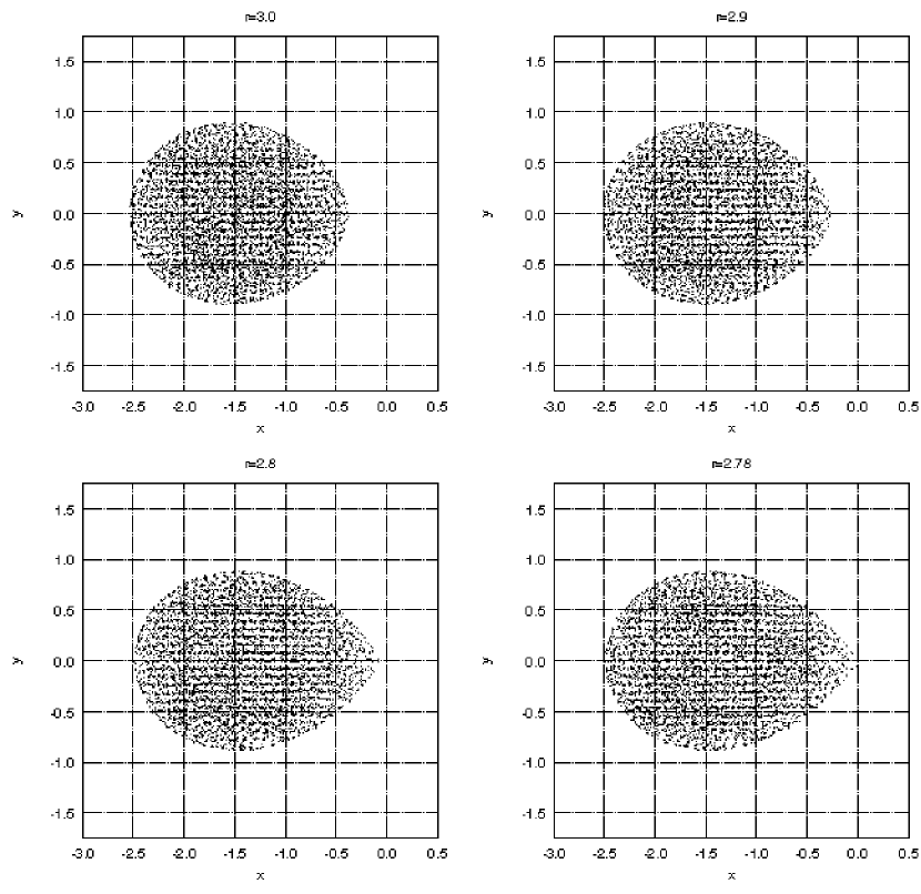
Figure 2: Particle positions projected onto the equatorial plane for initial configurations at various binary separations. One dot is plotted for every SPH particle.

plots of particle positions projected onto the equatorial plane for different separations. As the separation is decreased, the effect of the tidal potential becomes more apparent and the neutron star is distorted. The configuration at $r$=3.0 can be approximated by a tri–axial ellipsoid, while for those at $r$=2.8 and $r$=2.78 this is increasingly no longer the case.

5.2.2 Dynamical runs

We have used several of the configurations thus constructed to perform dynamical runs. In Figure 3

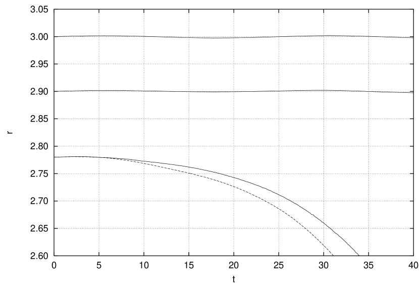
Figure 3: Binary separation as a function of time for dynamical calculations starting at three different separations ($r$=3.0, $r$=2.9 and $r$=2.78) for the black hole–neutron star binary with mass ratio $q$=1. For $r$=2.78, the solid line used $N$=8121 particles and the dotted line used $N$=16944 particles.

we show the binary separation as a function of time during several of these calculations. It is clear that the configurations with initial separations $r$=3.0 and $r$=2.9 are stable. The separation exhibits oscillations of numerical origin on a period close to the orbital period (respectively $P$=22.81 and $P$=21.6 in our units, see eq. [1]). However, the configuration with $r$=2.78 and initial period $P$=20.09 (corresponding to 37 km and 2.39 ms for $R$=13.4 km and $M$=$1.4M_{\odot}$) is unstable, and the separation decays on an orbital timescale. We find the dynamical stability limit to be $r_{dyn}$=2.78=$r_{RL}$. The two different lines with initial separation $r$=2.78 correspond to two different resolutions (the solid line used $N$=8121 particles and the dotted line used $N$=16944 particles). In the following, we will describe the results for our higher resolution run, with $N$=16944. In Figure 4

Figure 4: Density contours at various times during the dynamical coalescence of the black hole–neutron star binary with mass ratio $q$=1 and initial separation $r$=2.78. The logarithmic contours are evenly spaced every 0.25 decades, with the lowest one at $\log{\rho}=-3.25$. The rotation is counterclockwise and the initial orbital period is $P$=20.09. The left column shows density contours in the orbital plane, the right column shows contours in the meridional plane containing the binary axis. The black disk represents the black hole.

Figure 4: continued.

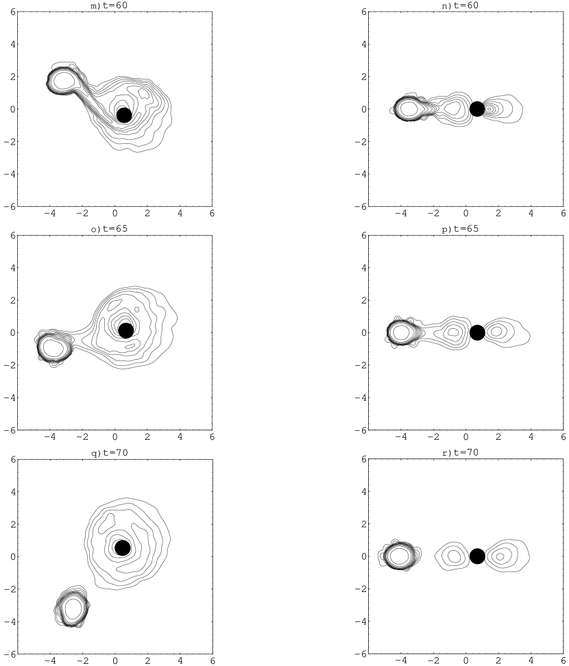
Figure 4: continued.

Figure 4: continued.

we show density contours at various times during the simulation, which was run from $t$=0 to $t$=100. The left column shows contours in the orbital plane, and the right column shows contours in the meridional plane containing the black hole and the center of mass of the SPH particles. The black disk with radius $r_{s}$ represents the black hole. Mass transfer from the neutron star to the black hole begins almost immediately (within one orbit) through the inner Lagrangian point. The accretion stream gradually becomes thicker and begins to wrap around the black hole. By $t$=50 the star has become considerably elongated and a toroidal structure has begun to form around the black hole. The accretion stream then essentially breaks, mass transfer stops and a stellar core remains in orbit around the black hole ($t$=60 through $t$=70). The result of this coalescence then appears to be a a stable binary with a greatly altered mass ratio and separation ($q_{final}$=0.19 and $r$$\sim$4.5, corresponding to 60 km), consisting of a remnant core with mass $M_{core}$=0.307 (corresponding to $0.43M_{\odot}$) in orbit around a black hole with $M_{BH}$=1.607 (or $2.25M_{\odot}$). The mass transfer event is very brief, as can be seen in Figure 5, where

Figure 5: Black hole mass (dotted line) and mass accretion rate onto the black hole (solid line) as a function of time for the black hole–neutron star binary with mass ratio $q$=1 and initial separation $r$=2.78.

we plot the mass of the black hole and the mass accretion rate onto the black hole as a function of time. The peak accretion rate is $dM_{BH}/dt$=0.0275 (corresponding to $0.3M_{\odot}/$ms). The black hole is still accreting matter towards the end of our simulation, but the decreased resolution (recall that accretion entails a loss of particles in the simulation) does not allow us to determine the distribution of matter accurately beyond $t$=100 ($\sim$11 ms). What can be determined is that the toroidal structure that forms does not extend to form a halo that engulfs the black hole completely. The region directly above the black hole remains devoid of matter down to the limit of our resolution of $7.1\times 10^{-5}$ (or $10^{-4}M_{\odot}$) within $\sim 5^{\rm o}$. The accretion structure around the black hole was not previously observed (Lee & Kluźniak (1995)) because of the low resolution ($N$=2176 particles) of our initial runs.

The nature of the encounter is reflected in the gravitational radiation waveforms, presented in Figure 6 (top).

Figure 6: Top: Gravitational radiation waveforms for the coalescence of a black hole–neutron star binary with mass ratio $q$=1. Two polarizations ($h_{+}$, left panel; $h_{\times}$, right panel) in geometrized units (such that $G$=$c$=1) are shown. Bottom: Gravitational radiation luminosity in geometrized units ($G$=$c$=1) for the coalescence of a black hole–neutron star binary (solid line) and a double neutron star binary (dotted line) with mass ratio $q$=1. The constant $L_{0}$=$c^{5}/G$=$3.6\times 10^{59}$ erg s^-1.

The amplitude of the emitted waves initially rises from $(r_{0}R/M^{2})h$=1.55 to $(r_{0}R/M^{2})h_{max}$=1.75, reflecting the decrease in separation. The subsequent drop in amplitude and decrease in frequency are a result of the short episode of mass transfer, and the final waveforms reflect the fact that the binary has survived the encounter (the new binary orbital period is $P\approx 39$ in our units, or 4.5 ms). Thus the presence of a remnant core in orbit around the black hole would be immediately apparent from an observation of the waveforms emitted during such a coalescence. We also show the gravitational wave luminosity in Figure 6 (bottom). For comparison purposes, the luminosity for the coalescence of two identical neutron stars is plotted as well, from the results of section 4.1. The maximum luminosity and total energy radiated in gravitational waves are $(R/M)^{5}L_{max}^{NS-NS}$=0.39 (or $1.17\times 10^{55}$ erg s^-1), $(R^{7/2}/M^{9/2})\Delta E_{GW}^{NS-NS}\approx 10$ (or $3.4\times 10^{52}$ erg) and $(R/M)^{5}L_{max}^{BH-NS}$=0.15 (or $4.5\times 10^{54}$ erg s^-1), $(R^{7/2}/M^{9/2})\Delta E_{GW}^{BH-NS}\approx 6$ (or $2\times 10^{52}$ erg) for the double neutron star and black hole–neutron star case respectively. Although in both cases there is still a clear rise and decay in the luminosity curve, the peak is much broader ($\Delta t^{BH-NS}\sim 25$) than for two neutron stars ($\Delta t^{NS-NS}\sim 15$). The slower rise in luminosity and longer timescale of the peak in the black hole–neutron star case are a direct consequence of having only one star being deformed and disrupted through tidal interactions.

Finally, we show in Figure 7

Figure 7: Binary separation for the coalescence of a black hole–neutron star binary with mass ratio $q$=1 (solid line) and for a point–mass binary with the same mass ratio and initial separation decaying via the emission of gravitational waves in the quadrupole approximation (dotted line).

the binary separation as a function of time for the simulation we have just presented, together with a plot of the separation for a point–mass binary with the same mass ratio and initial separation decaying via the emission of gravitational waves in the quadrupole approximation. This last curve is given by (e.g. Shapiro & Teukolsky (1983)) $r=r_{i}\left(1-t/t_{0}\right)^{1/4},$ where $t_{0}=(5r_{i}^{4}c^{5})/(256\mu M_{t}^{2}G^{3})$ and $r_{i}$ is the initial separation at $t$=0. The total mass is $M_{t}$=$M_{BH}$+$M$ and the reduced mass is $\mu$=$M_{BH}M/M_{t}$. Clearly, hydrodynamical effects and the instability they induce drive the coalescence process on a time scale that is shorter than that purely due to gravitational radiation losses, and so we may safely neglect the effect of radiation reaction on the evolution of the system over the time period which we have modeled.

In the calculation described above, we have integrated the thermal energy equation according to the first law of thermodynamics by setting

$$\Delta U=\Delta W+\Delta Q$$ (4)

where $\Delta Q$ is calculated using the contribution from the artifical viscosity (see equation A4 in Appendix A). We will denote this as Case I. To investigate the effect of radiative losses on the outcome of this configuration, we have performed an additional calculation for the extreme case in which all the energy produced by viscosity is lost by the system (e.g. to neutrinos). This will be denoted as Case II, and is achieved by simply removing the term associated with viscous heating from equation (4), so that we now have $\Delta U$=$\Delta W$. Density contours for Case II (with $N$=16944 particles) are shown in Figure 8

Figure 8: Density contours for the dynamical coalescence of the black hole–neutron star binary with mass ratio $q$=1 and initial separation $r$=2.78, Case II. There are eleven evenly spaced logarithmic contours down from $\log{\rho}=-0.75$ every 0.25 decades. The rotation is counterclockwise and the initial orbital period is $P$=20.09. The left column shows density contours in the orbital plane, the right column shows contours in the meridional plane containing the binary axis. The black disk represents the black hole.

for $t$=60 and $t$=80. An accretion torus is again clearly visible, and comparing with the contours in Figure 4 for Case I, the ring is clearly more confined both in the orbital plane and along the $z$-axis. This is clearly a consequence of a lack of pressure support due to the removal of thermal energy from the system. In Figure 9

Figure 9: The thermal energy loss rate due to viscosity $L_{v}$ in geometrized units (such that $G$=$c$=1), normalized to $L_{0}$=$c^{5}/G$=$3.6\times 10^{59}$ erg s^-1, as a function of time for an initial configuration with a mass ratio $q$=1 and initial separation $r$=2.78, Case II.

we show the rate of energy loss, $L_{v}$ due to viscous heating. The peak rate is $(R/M)^{5}L_{v}\approx 0.65$, corresponding to $\approx 2\times 10^{55}$ erg s^-1 and the total energy loss from $t$=0 to $t$=100 is $\approx 5\times 10^{52}$ erg. The mass transfer rate and gravitational radiation waveforms are essentially the same as for Case I. There is once more a baryon–free axis along the rotation axis of the binary, only this time it is clear of matter within $\sim 20^{\rm o}$ (down to $4\times 10^{-5}$, equivalent to $6\times 10^{-5}M_{\odot}$) since the torus is more nearly confined to the orbital plane.

5.3 Mass ratio $q$=0.8

5.3.1 Equilibrium configurations

For a mass ratio $q$=0.8, the black hole mass is $M_{BH}$=1.25 (or 1.75$M_{\odot}$). Hydrodynamical effects are still important in the construction of equilibrium configurations in this case, as can be seen in

Figure 10: Total angular momentum vs. binary separation for a black hole–neutron star binary with mass ratio $q$=0.8. The solid line is the result of the analytical approach of Lai, Rasio & Shapiro 1993b treating the neutron star as a compressible tri–axial ellipsoid, and the crosses are the result of SPH relaxation calculations. The Roche limit is at $r$=2.935.

Figure 10, where we have plotted the equilibrium angular momentum values for a range of binary separations. Approximating the neutron star as a compressible tri–axial ellipsoid gives results which are close to the full numerical calculations before the minimum in angular momentum is reached, but for $r\leq 3.0$ this is no longer the case. We identify the separation with minimum angular momentum at $r$=2.98, and Roche–Lobe overflow occurs at $r_{RL}$=2.935. For this value of the mass ratio $N$=8121 particles model the neutron star.

5.3.2 Dynamical runs

As for the case with $q$=1, several equilibrium configurations were used as initial conditions for dynamical runs. Figure 11 shows

Figure 11: Binary separation as a function of time for dynamical calculations starting at $r$=2.98 (solid line) and $r$=2.935 (dotted line) for the black hole–neutron star binary with mass ratio $q$=0.8.

the binary separation as a function of time for these calculations. The initial configuration with separation $r$=2.935 becomes unstable on a dynamical time scale. However, it is apparent that the development of the instability (and hence the orbital decay) proceeds at a slower rate than for a higher mass ratio. The reason for this is that since the black hole is more massive, Roche–Lobe overflow occurs at a greater separation than previously observed (for $q$=1), and so the tidal effects are less pronounced on the neutron star. Density contours in the orbital plane for the binary with initial separation $r$=2.935 are

Figure 12: Density contours in the orbital plane for a black hole–neutron star coalescence with a mass ratio $q$=0.8 and initial separation $r$=2.935. The logarithmic contours are evenly spaced every 0.25 decades, with the lowest one at $\log{\rho}=-2.75$. The black disk represents the black hole. Orbital rotation is counterclockwise and the initial orbital period is $P$=20.58.

Figure 12: continued.

shown in Figure 12. Mass transfer proceeds through the formation of an accretion stream from the neutron star to the black hole, lasting from $t$$\sim$45 to $t$$\sim$75 (about 3.5 ms), with a peak accretion rate of 0.017 (0.2$M_{\odot}$/ms). A substantial amount of mass is stripped from the neutron star during the encounter (see Figure 13), and

Figure 13: Black hole mass (dotted line) and mass accretion rate onto the black hole (solid line) as a function of time for the black hole–neutron star binary with mass ratio $q$=0.8 and initial separation $r$=2.935.

the final black hole mass is $M_{BH}$=1.65 (equivalent to 2.3$M_{\odot}$). The core of the neutron star, with a final mass $M_{core}$=0.595 (corresponding to 0.83$M_{\odot}$) again survives the encounter. However, the most striking difference between this case and the one presented previously ($q$=1) is the absence of a toroidal accretion structure around the black hole. All matter stripped from the neutron star is directly accreted by the black hole, and thus in this scenario as well the rotation axis above the black hole is devoid of matter. As a result of mass transfer the binary separation increases to $r$$\sim$3.6 and thus the final configuration in this case is again a stable binary.

As before, the hydrodynamical evolution of the binary is reflected in the gravitational radiation waveforms, presented in Figure 14 (top).

Figure 14: Top: Gravitational radiation waveforms for the coalescence of a black hole–neutron star binary with mass ratio $q$=0.8. Two polarizations ($h_{+}$, left panel; $h_{\times}$, right panel) in geometrized units (such that $G$=$c$=1) are shown. Bottom: Gravitational radiation luminosity in geometrized units ($G$=$c$=1) for the coalescence of a black hole–neutron star binary with mass ratio $q$=0.8. The constant $L_{0}$=$c^{5}/G$=$3.6\times 10^{59}$ erg s^-1.

There is an initial rise in amplitude in the waveforms, followed by a rapid decline and increase in the period, reflecting the episode of mass transfer and subsequent increase in binary separation. The peak amplitude in this case is $(r_{0}R/M^{2})h_{max}$=1.93, and again since the binary survives the encounter, the final amplitude is not zero but $(r_{0}R/M^{2})h_{final}$=1.25. The luminosity emitted in gravitational waves is shown in Figure 14 (bottom). The general shape of the curve resembles very much that for $q$=1, as one can expect after studying the density contour plots for each case (since the toroidal structure that was formed for $q$=1 is essentially azimuthally symmetric it does not contribute significantly to the emission of gravitational waves). The curve presents again a broad peak, with a duration $\Delta t$$\sim$30 (3.4 ms). The peak luminosity is $(R/M)^{5}L_{max}$=0.16 (or $4.8\times 10^{54}$ erg s^-1) and the total energy radiated away in gravitational waves is $(R^{7/2}/M^{9/2})\Delta E_{GW}$$\approx$$10$ (or $3.4\times 10^{52}$ erg). These values are higher than for the case with $q$=1 because we have normalized our results to the mass of neutron star, and lowering the mass ratio implies the system has a greater total mass.

In Figure 15

Figure 15: Binary separation for the coalescence of a black hole–neutron star binary with mass ratio $q$=0.8 (solid line) and for a point–mass binary with the same mass ratio and initial separation decaying via the emission of gravitational waves in the quadrupole approximation (dotted line).

we compare (as for $q$=1 in Figure 7) the orbital decay of this binary with that for a point–mass binary emitting gravitational waves in the quadrupole approximation. It is apparent that hydrodynamical effects are less important than for $q$=1 in determining the initial orbital evolution, but are nevertheless substantial.

5.4 Mass ratio $q$=0.31

Continuing the trend towards lower mass ratios, we chose a value of $q$=0.31, giving $M_{BH}$=3.22 (corresponding to 4.51$M_{\odot}$) to study the evolution of a binary system where most of the mass is contained in the black hole. We again used $N$=8121 particles to model the neutron star. A qualitative difference appears in the plot of total angular momentum as a function of binary separation (Figure 16).

Figure 16: Total angular momentum vs. binary separation for a black hole–neutron star binary with mass ratio $q$=0.31. The solid line is the result of the analytical approach of Lai, Rasio & Shapiro 1993b treating the neutron star as a compressible tri–axial ellipsoid, and the crosses are the result of SPH relaxation calculations. The Roche limit is at $r$=3.76. Note that Roche–Lobe overflow is reached before the minimum in angular momentum.

At a separation of $r$=3.76 (or 50.5 km), Roche–Lobe overflow occurs, so that we cannot construct a sequence with decreasing separation and constant mass ratio anymore, but this point is reached before the minimum in total angular momentum is attained, contrary to what occurred for $q$=1 and $q$=0.8. Thus we expect all configurations down to the Roche limit $r_{RL}$=3.76 to be dynamically stable (see the discussion for $q$=1 in Section 5.2.1).

The binary separation for a dynamical run with an initial separation $r$=$r_{RL}$=3.76 is shown in Figure 17.

Figure 17: Binary separation as a function of time for a dynamical calculation starting at $r$=3.76 for the black hole–neutron star binary with mass ratio $q$=0.31.

The initial orbital period is $P$=21.92 (or 2.51 ms). There is no longer orbital decay, but rather a slow increase in separation. This is simply due to the fact that there is slow Roche–Lobe overflow from the neutron star onto the black hole, transferring $\Delta M$=0.0104 (or 0.0146$M_{\odot}$) over $\sim$4.5 orbital periods. The neutron star is not disrupted at all during this process, as can be seen in Figure 18,

Figure 18: Density contours at various times during the dynamical coalescence of the black hole–neutron star binary with mass ratio $q$=0.31 and initial separation $r$=3.76. The logarithmic contours are evenly spaced every 0.25 decades, with the lowest one at $\log{\rho}$=-3.0. The rotation is counterclockwise and the initial orbital period is $P$=21.92. The black disk represents the black hole.

where we plot density contours in the orbital plane over the course of the simulation, and in Figure 19,

Figure 19: Gravitational radiation waveforms for the coalescence of a black hole–neutron star binary with mass ratio $q$=0.31. One polarization ($h_{+}$) in geometrized units (such that $G$=$c$=1) is shown.

where we plot the gravitational radiation waveform $h_{+}$ for this case. In fact, mass transfer is essentially conservative (i.e. the total angular momentum is conserved), and this approximation alone can accurately account for the change in separation. To see this, consider the following. Conservative mass transfer in a point–mass binary satisfies $J=\mu\Omega a^{2}=constant$, where a is the separation and $\mu$ is the reduced mass. Since the total mass is conserved and $\Omega\propto a^{-3/2}$ for a Keplerian binary, we find that $(M_{BH}M)^{2}a=constant$. For the black hole–neutron star binary with initial mass ratio $q$=0.31, we find that

$$\left[\frac{(M_{BH}M)_{initial}}{(M_{BH}M)_{final}}\right]^{2}=1.01453$$

and

$$\frac{a_{final}}{a_{initial}}=1.0167.$$

This is consistent with having conservative mass transfer despite the fact that the black hole–neutron star binary is not Keplerian. Angular momentum is practically constant since there is very little accretion, and this represents the only loss of angular momentum (via a spinning up of the black hole, which we do not model).

This last case is a clear indication of the limitations of the present method of studying the coalescence of a black hole with a neutron star. In the first place, since the orbit does not decay due to hydrodynamical effects, gravitational radiation reaction (which would drive the binary mentioned above to coalesce in a time $t_{0}$=31.35, correponding to 3.59 ms) cannot be ignored. Second, as is apparent in the density contour plots shown in Figure 18, the black hole has become almost as large as the neutron star itself (the Schwarschild radius is $r_{s}$=0.986, or 13.2 km, at the start of the simulation), making the radius of the innermost circular stable orbit (ISCO) $r_{ISCO}$=$3r_{s}$=2.958 (or 39.75 km). This means a substantial fraction of the neutron star is already at a distance $r\leq r_{ISCO}$ from the black hole. Thus including relativistic effects in this case becomes necessary in order to obtain meaningful results.

6 Discussion

We present in Table 2 the binary separations $r_{RL}$ and $r_{min}$, corresponding to the Roche limit and to the equilibrium configuration with minimum total angular momentum $J$ for each mass ratio. The lack of an entry for $r_{min}$ when $q$=0.31 reflects the fact that the orbits are stable when the separation is greater than that required for Roche–Lobe overflow.

In Table 3 we present a summary for the three configurations we explored in this paper, as well as for the coalescence of two identical neutron stars. The first column indicates if the coalescence involves two neutron stars or one neutron star and one black hole; the second and third columns show the initial and final mass ratios respectively; the fourth column indicates whether an accretion torus was formed; the fifth, sixth and seventh columns show the maximum and final gravitational radiation amplitude and the maximum gravitational radiation luminosity respectively, all in geometrized units such that $G$=$c$=1; the eighth column shows the mass of the central object for the case of the double neutron star coalescence, and that of the remnant core in the case of the black hole–neutron star coalescence.

Note that only in the simulation with a high mass ratio ($q$=1) did an accretion structure appear around the black hole. Otherwise, all matter stripped from the neutron star was directly accreted by the black hole. A striking result is that in every case, the neutron star is not completely disrupted, but a remnant core survives in orbit around the more massive black hole. Due to the violent mass transfer episode (for $q$=0.8 and $q$=1), this core is transferred to a higher orbit on a time scale of one orbit. For now, we are unable to model the system on longer time scales than we have presented here, but presumably the emission of gravitational waves will make the orbit decay by decreasing the separation. Clearly mass transfer will occur before the separation reaches zero, as soon as the neutron star overflows its Roche Lobe. For the equation of state we have considered (with $\Gamma$=3), the mass–radius relationship is $R\propto M^{1/5}$ and one can estimate the size of the Roche Lobe as $R_{RL}$=0.46$a(M/M_{t})^{1/3}$ (Paczyński (1967)). Using the rate of angular momenutum loss calculated from the quadrupole approximation, given by (Shapiro & Teukolsky (1983))

$$\frac{dJ}{dt}=-\frac{32}{5}\frac{G^{3}M_{t}^{2}\mu}{c^{5}a^{4}},$$

we can find the separation at which mass transfer will begin anew, as well as the time it will take for the orbit to shrink to this size. Applying this reasoning to the binary with initial $q$=1 after the initial mass transfer event, we find that a second episode of mass transfer will occur $\sim$40 ms later, and for the case with initial $q$=0.8, the delay will be $\sim$4 ms. Thus the length of the coalescence process is extended from a few milliseconds to possibly several tens of milliseconds.

Another important result is the fact that in every case, there is a baryon–free line of sight to the black hole along the rotation axis of the binary throughout the simulation. As stated in section 5.2.2, the limit we infer for the amount of matter along this axis from our calculations is $10^{-4}M_{\odot}$ within about 5^o of the rotation axis. It is set by the resolution in our calculation and thus represents an upper bound at this point. For the calculations with a lower mass ratio ($q$=0.8 and $q$=0.31) there was no visible accretion structure present around the black hole, and so the rotation axis was clear of matter as well. These last two results may make the coalescence of a black hole with a neutron star a promising candidate source for the production of GRBs (Kluźniak & Lee (1998)).

The survival of the neutron star core suggests a different outcome than what was initially expected for the coalescence of a black hole with a neutron star (Wheeler (1971)), and identifies this process as the only one known capable of producing low–mass neutron stars. The violent episode of mass transfer strips the neutron star of so much matter that it may drive it below the minimum mass required for stability. If this happens, then the core explodes (Blinnikov et al. (1984); Sumiyoshi et al. (1998); Colpi, Shapiro & Teukolsky (1991)) in approximately 0.1 seconds after a slow expansion phase that may last 20 seconds (Sumiyoshi et al. (1998)). The presence of the black hole would complicate the outcome of this event.

Appendix A Numerical Code

The equations of motion in SPH are essentially those of an N–body problem, with each particle representing a fluid element. Thus the equations for particle i can be written as:

$$\dot{\mbox{\boldmath$r$}}_{i}=\mbox{\boldmath$v_{i}$},$$

$$m_{i}\dot{\mbox{\boldmath$v$}}_{i}=\mbox{\boldmath$F_{iG}$+$F_{iH}$},$$

where $r_{i}$, $v_{i}$ and m_i are the position, velocity and mass of particle i respectively, and $F_{iG}$ and $F_{iH}$ denote the gravitational and hydrodynamic forces. The density at the position of particle i is

$$\rho_{i}\equiv\rho(\mbox{\boldmath$r_{i}$})=\sum_{j}m_{j}W_{ij},$$

where $W_{ij}$ is the symmetrized kernel for particles i and j. With $h_{i}$ representing the smoothing length for particle i, we have

$$W_{ij}=W(\mid\mbox{\boldmath$r_{i}-r_{j}$}\mid,h_{ij}),\ h_{ij}=\frac{1}{2}(h_{i}+h_{j}).$$

It is convenient to perform calculations with a kernel that has compact support. We use the form of Monaghan & Lattanzio (1985):

$$W(r,h)=\frac{1}{\pi h^{3}}\left\{\begin{array}[]{ll}1-\frac{3}{2}\left(\frac{r}{h}\right)^{2}+\frac{3}{4}\left(\frac{r}{h}\right)^{3},&0\leq r/h<1,\\ \frac{1}{4}\left(2-\frac{r}{h}\right)^{3},&1\leq r/h<2,\\ 0,&2\leq(r/h).\end{array}\right.$$

To obtain a value of the pressure for any particle, we use the equation of state. For an ideal gas this becomes

$$P_{i}=(\Gamma-1)u_{i}\rho_{i},$$

where $\Gamma$ is the adiabatic index and $u_{i}$ is the thermal energy per unit mass for particle i.

$F_{iH}$ includes the contribution from the pressure gradient and from artificial viscosity. In symmetrized form, it can be written as

$$\mbox{\boldmath$F_{iH}$}=-\sum_{j}m_{j}m_{i}\left(2\frac{\sqrt{P_{i}P_{j}}}{\rho_{i}\rho_{j}}+\Pi_{ij}\right)\mbox{\boldmath$\nabla$}_{i}W_{ij},$$ (A2)

where

$$\Pi_{ij}=\left\{\begin{array}[]{ll}(-\alpha\overline{c}_{ij}\mu_{ij}+\beta\mu_{ij}^{2})/\overline{\rho}_{ij},&\mbox{\boldmath$v_{ij}$}\cdot\mbox{\boldmath$r_{ij}$}<0\\ 0,&\mbox{\boldmath$v_{ij}$}\cdot\mbox{\boldmath$r_{ij}$}>0\end{array}\right.,$$

$$\mu_{ij}=\frac{h_{ij}(\mbox{\boldmath$v_{ij}$}\cdot\mbox{\boldmath$r_{ij}$})}{r_{ij}^{2}+\eta^{2}h_{ij}^{2}}.$$

Here $v_{ij}$=$v_{i}$$-$$v_{j}$, $r_{ij}$=$r_{i}$$-$$r_{j}$, $\alpha$ and $\beta$ are constants, $c_{i}$ is the speed of sound at the position of particle i, and $\overline{c}_{ij}$=$(c_{i}+c_{j})/2$ and $\overline{\rho}_{ij}$=$(\rho_{i}+\rho_{j})/2$. In the simulations presented in this paper we have used $\alpha$=1, $\beta$=2 and $\eta^{2}$=$10^{-2}$.

The form of $F_{iH}$ , and in particular the symmetrization of the pressure gradient term, ensures that forces between pairs of particles are symmetric, and so linear and angular momentum are automatically conserved. The viscosity is introduced with a term linear in the velocity differences, which produces shear and bulk viscosity, and a quadratic term to handle high Mach numbers in shocks, analogous to the Von Neumann–Richtmyer artificial viscosity used in finite–difference methods (Richtmyer (1967)).

The value $u_{i}$ of the thermal energy per unit mass is evolved in time according to the the first law of thermodynamics, taking into account the contribution from the viscous terms. The symmetrized form is:

$$\frac{du_{i}}{dt}=\frac{1}{2}\sum_{j}m_{j}\left(2\frac{\sqrt{P_{i}P_{j}}}{\rho_{i}\rho_{j}}+\Pi_{ij}\right)\mbox{\boldmath$v_{ij}$}\cdot\mbox{\boldmath$\nabla$}_{i}W_{ij}.$$ (A4)

The thermal energy equation is integrated by essentially using a two–step procedure (Hernquist & Katz (1989)) in order to preserve accuracy. This is necessary because the heating rate depends on the pressure, and via the equation of state, on the thermal energy itself.

Individual smoothing lengths $h_{i}$ are adjusted so that every particle has an approximately constant number $\nu$ of hydrodynamical neighbors, i.e., those for which $r_{ij}/h_{ij}\leq 2$. This ensures that adequate spatial resolution is maintained and that the level of accuracy of the interpolations remains uniform throughout the fluid. If $h_{i,n}$ is the smoothing length for particle i at step n, the value at step $n+1$ is found according to (Hernquist & Katz (1989)):

$$h_{i}^{n+1}=\frac{h_{i}^{n}}{2}\left[1+\left(\frac{\nu}{\nu^{n}}\right)^{\frac{1}{3}}\right],$$ (A5)

where $\nu^{n}$ is the number of hydrodynamical neighbors at step n. We have found that a value of $\nu$=64 yields adequate sampling of the fluid without requiring excessive computation time.

Gravitational force calculations constitute the most time–consuming part of an $N$–body code. A direct calculation requires $O(N^{2})$ operations, and this becomes prohibitive as the number of particles is increased above a few hundred. In order to make this process more efficient we have incorporated a binary tree structure (Hernquist & Katz (1989)) into our code to obtain gravitational forces. This makes the number of required operations of $O(N\log N$), thus allowing for simulations with several thousand particles. The tree structure is built by pairing two particles into a new pseudo–particle, called a node, if they are mutual nearest neighbors, and proceeding with this pairing over all particles and newly created nodes until there is only one node, at the center of mass of the particles being considered. This hierarchical association makes up the binary tree which we use to compute the forces (for a detailed description see Benz et al. (1990)). The force on any particle can then be obtained by adding up contributions from particles close enough to be considered individually and by more distant aggregations, which can be described in terms of their multipolar expansion up to the quadrupole term. To decide if an aggregation of particles must be resolved to obtain the force on particle i, we consider the ratio $s/d$, where d is the distance from particle i to the aggregate and s is its size. If $s/d\geq\theta$, where $\theta$ is a dimensionless tolerance parameter, the aggregate is resolved further. If the converse is true, the contribution to the force is obtained from the quadrupole expansion. We adopt $\theta$=0.8, which provides an accuracy for the force of better than one part in $10^{2}$. However, the aggregate is resolved further if it contains any individual particles which may be hydrodynamical neighbors for particle i. The subroutine corresponding to this approach simultaneously provides $F_{iG}$ and the hydrodynamical neighbors for every particle that are used to obtain $F_{iH}$ and $du_{i}/dt$ in equations (A2) and (A4). Our calculations of the gravitational forces are completely Newtonian.

We use a leapfrog algorithm accurate to second order to integrate the equations of motion. The time step is adaptive, and is taken to satisfy a combination of the Courant criterion for stability and a further restriction on the maximum change allowed in velocity for any particle during one time step to conserve accuracy. We follow Monaghan (1989) and set the time step to be $\Delta t$=$\min{(\Delta t_{1},\Delta t_{2})}$ with

$$\Delta t_{1}=\min_{i}(h_{i}/\dot{v}_{i})^{1/2}$$

$$\Delta t_{2}=0.15\min_{i}\left(\frac{h_{i}}{c_{i}+1.2\alpha c_{i}+1.2\beta\max_{j}(\mu_{ij})}\right)$$

One of the main objectives of the present work is to investigate the gravitational waves emitted by coalescing binaries. In our Newtonian simulations we calculate the waveforms of the emitted waves and the total luminosity in the quadrupole approximation. The amplitude of the retarded wave at time t and a distance $r_{0}$ away from the source is given by  (Misner, Thorne & Wheeler (1970))

$$h^{TT}_{jk}=\frac{2}{r_{0}}\frac{G}{c^{4}}{\ddot{I\mkern-6.8mu\raise 1.29167pt\hbox{-}\mkern 6.0mu}\mkern-6.0mu}{}_{jk}\,^{TT}\left(t-\frac{r_{0}}{c}\right),$$

$$\mbox{where}\ I\mkern-6.8mu\raise 1.29167pt\hbox{-}_{jk}\,^{TT}=P_{jn}I\mkern-6.8mu\raise 1.29167pt\hbox{-}_{nm}P_{mk}-P_{jk}P_{lm}I\mkern-6.8mu\raise 1.29167pt\hbox{-}_{lm}/2$$

is the transverse traceless part of the reduced quadrupole moment,

$$I\mkern-6.8mu\raise 1.29167pt\hbox{-}_{jk}=I_{jk}-\delta_{jk}I,$$

$$\mbox{with}\ I_{jk}=\int\rho x_{j}x_{k}d\mbox{\boldmath$r$}$$

$$\mbox{and}\ I=\sum_{j}I_{jj}.$$

The $P_{ij}$ are the components of the projection operators onto the plane transverse to the radial direction: $P_{ij}=\delta_{ij}-n_{i}n_{j}$ with $n_{i}=x_{i}/r_{0}$.

The luminosity of the gravitational waves at a distance r from the source is

$$L_{GW}=\frac{dE}{dt}=\frac{1}{5}\frac{G}{c^{5}}\left\langle\frac{d{\ddot{I\mkern-6.8mu\raise 1.29167pt\hbox{-}\mkern 6.0mu}\mkern-6.0mu}{}_{jk}}{dt}\frac{d{\ddot{I\mkern-6.8mu\raise 1.29167pt\hbox{-}\mkern 6.0mu}\mkern-6.0mu}{}_{jk}}{dt}\right\rangle.$$ (A6)

We use the method of Finn (1989) and obtain the formula applicable to SPH for the second derivative of the quadrupole moment (Rasio & Shapiro (1992)):

$$\ddot{I}_{fluid}^{jk}=\sum_{i}m_{i}\left(2v_{i}^{j}v_{i}^{k}+\frac{2P_{i}}{\rho_{i}}\delta^{jk}+x_{i}^{k}g_{i}^{j}+x_{i}^{j}g_{i}^{k}\right).$$

The summation is over the SPH particles and the superscripts indicate the cartesian components. We identify the gravitational acceleration on particle i as $g_{i}$. The term $\ddot{I}_{fluid}^{jk}$ only includes the contribution from the SPH particles contained in the neutron star. We add the terms arising from the presence of the black hole as a point mass contribution:

$$\ddot{I}_{BH}^{jk}=M_{BH}\left(2v_{BH}^{j}v_{BH}^{k}+x_{BH}^{k}g_{BH}^{j}+x_{BH}^{j}g_{BH}^{k}\right),$$

to obtain the total value of $\ddot{I}$ as

$$\ddot{I}^{jk}=\ddot{I}_{BH}^{jk}+\ddot{I}_{fluid}^{jk}.$$

The gravitational waveforms are thus obtained directly from dynamical and hydrodynamical variables of the system, and one numerical differentiation of $\ddot{I}^{jk}$ is required to obtain the luminosity.

The amplitudes of the waveforms for an observer a distance $r_{0}$ away along the axis of rotation of the binary are given by

$$r_{0}h_{+}=\frac{G}{c^{4}}\left({\ddot{I\mkern-6.8mu\raise 1.29167pt\hbox{-}\mkern 6.0mu}\mkern-6.0mu}{}_{xx}-{\ddot{I\mkern-6.8mu\raise 1.29167pt\hbox{-}\mkern 6.0mu}\mkern-6.0mu}{}_{yy}\right),$$ (A7)

$$r_{0}h_{\times}=2\frac{G}{c^{4}}{\ddot{I\mkern-6.8mu\raise 1.29167pt\hbox{-}\mkern 6.0mu}\mkern-6.0mu}{}_{xy}.$$ (A8)

Table 1: Comparison of results for the coalescence of two identical polytropes with a stiff equation of state ($\Gamma=3$).

	$(r_{0}R/M^{2})h_{max}$	$(r_{0}R/M^{2})h_{final}$	$(R/M)^{5}(L_{max}/L_{0})$	$\rho_{c}$	$M_{halo}/M_{tot}$
This work	2.2	0.2	0.39	0.44	0.16
RS	2.2	0.2	0.37	0.40	0.18

Table 2: Critical Separations for black hole–neutron star binaries.

$q$	$r_{min}$	$r_{RL}$
1.00	2.82	2.78
0.80	2.97	2.94
0.31	$\cdots$	3.76

Table 3: Summary of results for the coalescence of two neutron stars and a black hole with a neutron star.

	$q_{i}$	$q_{f}$	Torus	$(r_{0}R/M^{2})h_{max}$	$(r_{0}R/M^{2})h_{final}$	$(R/M)^{5}(L_{max}/L_{0})$	$M_{core}$
NS–NS	1.000	1.000	no	2.20	0.20	0.390	0.82
BH–NS	1.000	0.190	yes	1.75	0.55	0.145	0.3070
BH–NS	0.800	0.360	no	1.93	1.25	0.160	0.5950
BH–NS	0.310	0.306	no	3.59	3.48	0.425	0.9896

References

- Benz et al. (1990) Benz, W., Bowers, R.L., Cameron, A.G.W., Press, W.H. 1990, Astrophysical Journal, 348, 647.
- Bildsten & Cutler (1992) Bildsten, L., Cutler, C. 1992, Astrophysical Journal, 400, 175.
- Blinnikov et al. (1984) Blinnikov, S.I., Novikov, I.D., Perevodchikova, T.V., Polnarev, A.G. 1984, Soviet Astronomy Letters, 10(3), 177.
- Coleman & Bicknell (1985) Coleman, C.S., Bicknell, G.V. 1985, Monthly Notices of the Royal Astronomical Society, 214, 337.
- Colpi, Shapiro & Teukolsky (1991) Colpi, M., Shapiro, S.L., Teukolsky, S.A. 1991, Astrophysical Journal, 369, 422.
- (6) Davies, M.B., Benz, W., Piran, T., Thielemann, F.K. 1994, Astrophysical Journal, 431, 742.
- Eichler, Livio, Piran & Schramm (1988) Eichler, D., Livio, M., Piran, T., Schramm, D.N. 1988, Nature, 340, 126.
- Finn (1989) Finn, L.S. 1989, in Frontiers of Numerical Relativity, ed. C.R. Evans, L.S. Finn & D.W. Hobill (Cambridge: Cambridge Univ. Press), 126
- Fishman & Meegan (1995) Fishman, G.J., Meegan, C.A. 1995, Annual Review of Astronomy and Astrophysics, 33, 415.
- Gingold & Monaghan (1977) Gingold, R.A., Monaghan J.J. 1977, Monthly Notices of the Royal Astronomical Society, 181, 375.
- Hernquist & Katz (1989) Hernquist, L., Katz, N. 1989, Astrophysical Journal Supplement, 70, 419.
- Hulse & Taylor (1975) Hulse, R.A., Taylor, J.H., 1975, Astrophysical Journal, 195, L51
- Janka & Ruffert (1996) Janka, H.T., Ruffert, M. 1996, Astronomy and Astrophysics, 307, L33.
- Kluźniak & Lee (1998) Kluźniak, W., Lee, W.H., Astrophysical Journal Letters, 494, L53, 1998.
- (15) Lai, D., Rasio, F.A., Shapiro, S.L. 1993a, Astrophysical Journal Letters, 406, L63.
- (16) Lai, D., Rasio, F.A., Shapiro, S.L. 1993b, Astrophysical Journal Supplement, 88, 205.
- Lattimer & Schramm (1976) Lattimer, J.M., Schramm, D.N. 1976, Astrophysical Journal, 210, 549.
- Lee (1998) Lee, W.H. 1998, PhD Thesis, University of Wisconsin–Madison.
- Lee & Kluźniak (1995) Lee, W.H., Kluźniak, W. 1995, Acta Astronomica, 45, 705.
- Lucy (1977) Lucy, L. 1977, Astronomical Journal, 82, 1013
- Metzger et al. (1997) Metzger, M.R. et al. 1997, Nature 387, 878.
- Mészáros & Rees (1992) Mészáros, P., Rees, M.J. 1992, Monthly Notices of the Royal Astronomical Society, 257, 29P.
- (23) Mészáros, P., Rees, M.J. 1993, Astrophysical Journal, 405, 278.
- Misner, Thorne & Wheeler (1970) Misner, C.W., Thorne, K.S., Wheeler, J.A. 1970, Gravitation (NY:Freeman).
- Monaghan (1989) Monaghan, J.J. 1989, J. Comput. Phys., 82, 1.
- Monaghan (1992) Monaghan, J.J. 1992, Annual Review of Astronomy and Astrophysics, 30, 543.
- Monaghan & Gingold (1983) Monaghan J.J., Gingold, R.A. 1983, Journal of Computational Physics, 52, 375.
- Monaghan & Lattanzio (1985) Monaghan J.J., Lattanzio, J.C. 1985, Astronomy and Astrophysics, 149, 135.
- (29) Nakamura, T., Oohara, K. 1989, Progress of Theoretical Physics, 82, 1066.
- Narayan, Paczyński & Piran (1992) Narayan, R., Paczyński, B., Piran, T. 1992, Astrophysical Journal, 395, L83.
- Narayan, Piran & Shemi (1991) Narayan, R., Piran, T., Shemi, A. 1991, Astrophysical Journal Letters, 379, L17.
- (32) Oohara, K., Nakamura, T. 1989, Progress of Theoretical Physics, 82, 535.
- (33) Oohara, K., Nakamura, T. 1990, Progress of Theoretical Physics, 83, 906.
- Paczyński (1967) Paczyński, B. 1967, Acta Astronomica, 17, 287.
- Paczyński (1986) Paczyński, B. 1986, Astrophys. J., 308, L43.
- Paczyński (1991) Paczyński, B. 1991, Acta Astronomica, 41, 257.
- Rasio & Shapiro (1992) Rasio, F., Shapiro, S.L. 1992, Astrophysical Journal, 401, 226.
- Rasio & Shapiro (1994) Rasio, F., Shapiro, S.L. 1994, Astrophysical Journal, 432, 242.
- Richtmyer (1967) Richtmyer, R.D., Morton, K.W., 1967, Difference Methods for Initial–Value Problems (New York, Wiley)
- (40) Ruffert, M., Janka, H.-Th., Schäfer, G. 1996, Astronomy and Astrophysics, 311, 532.
- (41) Ruffert, M., Janka, H.-Th., Takahashi, K., Schäfer, G. 1997a, Astronomy and Astrophysics, 319, 122.
- (42) Ruffert, M., Rampp, M., Janka, H.-Th. 1997b, Astronomy and Astrophysics, 321, 991.
- Shapiro & Teukolsky (1983) Shapiro, S.L., Teukolsky, S.A. 1983, Black Holes, White Dwarfs and Neutron Stars, Wiley–Interscience.
- Sumiyoshi et al. (1998) Sumiyoshi, K., Yamada, S., Suzuki, H., Hilldebrandt, W., Astronomy and Astrophysics, 334, 159, 1998.
- Taylor & Weisberg (1982) Taylor, J.H., Weisberg, J.M. 1982, Astrophysical Journal, 253, 908.
- Taylor et al. (1992) Taylor, J.H., Wolszczan, A., Damour, T., Weisberg, J.M., 1992, Nature, 355, 132.
- Thorne (1995) Thorne, K.S. 1995, in Proceedings of the Snowmass 95 Summer Study on Particle and Nuclear Astrophysics and Cosmology, eds. E.W. Kolb and R. Peccei (World Scientific, Singapore).
- Wheeler (1971) Wheeler, J.A. 1971, Pontificae Acad. Sci. Scripta Varia, 35, 539.
- Wilson, Salmonson & Mathews (1997) Wilson, J.R., Salmonson, J.D., Mathews, G.J. 1997, in Gamma Ray Bursts, C.A. Meegan, R.D. Preece, T.M. Koshut, eds., (AIP: New York), 788.
- Wilson, Mathews & Maronetti (1996) Wilson, J.R., Mathews, G.J., Maronetti, P. 1996, Physical Review D, 54, 1317.
- Wolszczan (1991) Wolszczan, A., 1991, Nature, 350, 688.
- Żurek & Benz (1986) Żurek, W.H., & Benz, W. 1986, Astrophysical Journal, 308, 123.