Merger of black hole-neutron star binaries in full general relativity

Abstract

We present our latest results for simulation for merger of black hole (BH)-neutron star (NS) binaries in full general relativity which is performed preparing a quasicircular state as initial condition. The BH is modeled by a moving puncture with no spin and the NS by the $\Gamma$-law equation of state with $\Gamma=2$ and corotating velocity field as a first step. The mass of the BH is chosen to be $\approx 3.2M_{\odot}$ or $4.0M_{\odot}$, and the rest-mass of the NS $\approx 1.4M_{\odot}$ with relatively large radius of the NS $\approx 13$–14 km. The NS is tidally disrupted near the innermost stable orbit but $\sim 80$–90% of the material is swallowed into the BH and resulting disk mass is not very large as $\sim 0.3M_{\odot}$ even for small BH mass $\sim 3.2M_{\odot}$. The result indicates that the system of a BH and a massive disk of $\sim M_{\odot}$ is not formed from nonspinning BH-NS binaries irrespective of BH mass, although a disk of mass $\sim 0.1M_{\odot}$ is a possible outcome for this relatively small BH mass range as $\sim 3$–4$M_{\odot}$. Our results indicate that the merger of low-mass BH and NS may form a central engine of short-gamma-ray bursts.

1 Introduction

Merger of black hole (BH)-neutron star (NS) binaries is one of likely sources of kilo-meter size laserinterferometric gravitational wave detectors. Although such system has not been observed yet in contrast to NS-NS binaries, statistical studies based on the stellar evolution synthesis suggest that the merger will happen more than 10% as frequently as the merger of binary NSs [1, 2]. Thus, the detection of such system will be achieved by laserinterferometers in near future. This motivates theoretical studies for the merger of BH-NS binaries.

According to a study based on the tidal approximation (which is referred to as a study for configuration of a Newtonian star in circular orbits around a BH in its relativistic tidal field; e.g., [3, 4, 5, 6, 7]), the fate is classified into two cases, depending on the mass ratio $q\equiv M_{\rm NS}/M_{\rm BH}$, where $M_{\rm BH}$ and $M_{\rm NS}$ denote the masses of BH and NS, respectively. For $q\mathrel{\raise 1.29167pt\hbox{$<$}\mkern-14.0mu\lower 2.58334pt\hbox{$\sim$}}q_{c}$, the NS of radius $R$ will be swallowed into the BH horizon without tidal disruption before the orbit reaches the innermost stable circular orbit (ISCO) [5, 6]. On the other hand, for $q\mathrel{\raise 1.29167pt\hbox{$>$}\mkern-14.0mu\lower 2.58334pt\hbox{$\sim$}}q_{c}$, NS may be tidally disrupted before plunging into BH. Here, the critical value of $q_{c}$ depends on the BH spin and equation of state (EOS) of NS. For the nonspinning case with stiff EOSs, $q_{c}\approx 0.3$–$0.35(R/5M_{\rm NS})^{-3/2}$ and for the case that spin of a BH aligns with the orbital angular momentum, $q_{c}$ can be larger [6]. (Throughout this paper, we adopt the geometrical units $c=G=1$.)

The tidal disruption has been studied with great interest because of the following reasons. (i) Gravitational waves at tidal disruption will bring information about the NS radius since the tidal disruption limit depends sensitively on it [8]. The relation between the mass and the radius of NSs may be used for determining the EOS of high density matter [9]. (ii) Tidally disrupted NSs may form a massive disk of mass $\sim 0.1$–$1M_{\odot}$ around BH if the tidal disruption occurs outside the ISCO. Systems consisting of a rotating BH surrounded by a massive, hot disk have been proposed as one of likely sources for the central engine of gamma-ray bursts (GRBs) with a short duration [10], and hence, merger of low-mass BH and NS is a candidate.

However, the scenario based on the tidal approximation studies may be incorrect since gravitational radiation reaction and self-gravitational effects of NS to the orbital motion are ignored. Radiation reaction shortens the time available for tidally disrupting NSs. The gravity of NS could increase the orbital radius of the ISCO and hence the critical value of the tidal disruption, $q_{c}$, may be larger in reality. Miller [11] estimates these ignored effects and suggests that NSs of canonical mass and radius will be swallowed into BH without tidal disruption. Moreover, NSs are described by the Newtonian gravity in the tidal approximation. If we treat it in general relativity, the self-gravity is stronger and hence tidal disruption is less likely.

Tidal disruption of NSs by a BH has been investigated in the Newtonian [12] and approximately general relativistic (GR) simulation [13, 7]. However, the criterion of the tidal disruption will depend on GR effects as mentioned above, and hence, a simulation in full general relativity is obviously required (see [14] for an effort). In [15], we present our first numerical results for fully GR simulation, performed by our new code which has been improved from previous one [16, 17]; we handle an orbiting BH adopting the moving puncture method, which has been recently developed by two groups [18] (see also [19] for detailed calibration of this method). As the initial condition, we prepare a quasicircular state computed in a new formalism described in Sec. 2. Focusing particularly on whether NSs of realistic mass and radius is tidally disrupted to form a massive disk around nonspinning BHs, we illustrate that a disk with mass $\sim M_{\odot}$ is an unlikely outcome for plausible values of NS mass and radius and for BH mass greater than $3M_{\odot}$, although a disk of mass of $O(0.1M_{\odot})$ is possible.

In this paper, we extend previous study; we perform a simulation for different BH mass from that in [15] to find the dependence of the disk mass on the BH mass. In addition, gravitational waves are derived. The paper is organized as follows. In Sec. 2, we describe a formulation for computing quasicircular states in the moving-puncture framework. Section 3 presents some of numerical results for the quasicircular orbits. In Sec. 4, we report numerical results of simulations for the merger of BH-NS binaries. Section 5 is devoted to a summary and discussion.

2 Formalism for a quasicircular state

Three groups have worked in computing quasicircular states of BH-NS binaries [20, 21, 22]. However, this field is still in an early stage in contrast to computation for NS-NS binaries (e.g., [23]). In [15], we proposed a new method for computing accurate quasicircular states that can be used for numerical simulation in the moving puncture framework [24, 18]. Here, we briefly describe the formulation.

Even just before the merger, it is acceptable to assume that BH-NS binaries are in a quasicircular orbit since the time scale of gravitational radiation reaction is a few times longer than the orbital period. Thus, we assume the presence of a helical Killing vector around the mass center of the system, $\ell^{\mu}=(\partial_{t})^{\mu}+\Omega(\partial_{\varphi})^{\mu}$, where the orbital angular velocity $\Omega$ is constant.

In the present work, we assume that the NS is corotating around the mass center of the system for simplicity. Irrotational velocity field is believed to be more realistic for BH-NS binaries [25]. The work for the irrotational case will be reported in the future paper [26]. The assumption of corotating velocity field in the helical symmetric spacetime yields the first integral of the Euler equation, $h^{-1}u^{t}={\rm const}$, where $h$ is specific enthalpy defined by $1+\varepsilon+P/\rho$, and $\varepsilon$, $P$, and $\rho$ are specific internal energy, pressure, and rest-mass density, respectively. In the present work, we adopt the $\Gamma$-law EOS with $\Gamma=2$; $P=\rho\varepsilon=\kappa\rho^{2}$ with $\kappa$ an adiabatic constant. $u^{\mu}$ denotes the four velocity and $u^{t}$ its time component. Assumption of corotation implies $u^{\mu}=u^{t}\ell^{\mu}$ and thus $u^{r}=u^{\theta}=0$.

For a solution of geometric variables of quasicircular orbits, we adopt the conformal flatness formalism for three-geometry. In this formalism, the solution is obtained by solving Hamiltonian and momentum constraint equations, and an equation for the time slicing condition which is derived from $K_{k}^{~{}k}=0$ where $K_{ij}$ is the extrinsic curvature and $K_{k}^{~{}k}$ its trace [27]. Using the conformal factor $\psi$, the rescaled tracefree extrinsic curvature $\hat{A}_{i}^{~{}j}\equiv\psi^{6}K_{i}^{~{}j}$, and weighted lapse $\Phi\equiv\alpha\psi$ where $\alpha$ is the lapse function, these equations are respectively written

$$\Delta\psi=-2\pi\rho_{\rm H}\psi^{5}-{1\over 8}\hat{A}_{i}^{~{}j}\hat{A}_{j}^{~{}i}\psi^{-7},$$ (1)

$$\hat{A}^{~{}j}_{i~{},j}=8\pi J_{i}\psi^{6},$$ (2)

$$\Delta\Phi=2\pi\Phi\Big{[}\psi^{4}(\rho_{\rm H}+2S)+{7\over 16\pi}\psi^{-8}\hat{A}_{i}^{~{}j}\hat{A}_{j}^{~{}i}\Big{]},$$ (3)

where $\Delta$ denotes the flat Laplacian, $\rho_{\rm H}=\rho h(\alpha u^{t})^{2}-P$, $J_{i}=\rho hu_{i}$, and $S=\rho h[(\alpha u^{t})^{2}-1]+3P$.

We solve these equations in the framework of the puncture BH [24, 18, 28]. Assuming that the puncture is located at ${\mbox{\boldmath$r$}}_{\rm P}$, we set $\psi$ and $\Phi$

$$\psi=1+{M_{\rm P}\over 2r_{\rm BH}}+\phi\ \ \mbox{and}\ \ \Phi=1-{C\over r_{\rm BH}}+\eta,$$ (4)

where $M_{\rm P}$ and $C$ are positive constants, and $r_{\rm BH}=|x^{k}_{\rm BH}|$ ($x^{k}_{\rm BH}=x^{k}-x^{k}_{\rm P}$). Then elliptic equations for functions $\phi$ and $\eta$ are derived. The constant $M_{\rm P}$ is arbitrarily given, while $C$ is determined from the virial relation (e.g., [29])

$$\oint_{r\rightarrow\infty}\partial_{i}\Phi dS^{i}=-\oint_{r\rightarrow\infty}\partial_{i}\psi dS^{i}=2\pi M,$$ (5)

where $M$ is the ADM mass. The mass center is determined from the condition that the dipole part of $\psi$ at spatial infinity is zero. In this method, the region with $\alpha<0$ exists. However, this does not cause any pathology in the initial value problem.

Equation (2) is rewritten setting

$$\hat{A}_{ij}(=\hat{A}_{i}^{~{}k}\delta_{jk})=W_{i,j}+W_{j,i}-{2\over 3}\delta_{ij}\delta^{kl}W_{k,l}+K^{\rm P}_{ij},$$ (6)

where $K^{\rm P}_{ij}$ denotes the weighted extrinsic curvature associated with linear momentum of a puncture BH;

$$K^{\rm P}_{ij}={3\over 2r_{\rm BH}^{2}}\biggl{(}n_{i}P_{j}+n_{j}P_{i}+(n_{i}n_{j}-\delta_{ij})P_{k}n_{k}\biggr{)}.$$ (7)

Here, $n^{k}=n_{k}=x^{k}_{\rm BH}/r_{\rm BH}$. $P_{i}$ denotes linear momentum of the BH, determined from the condition that the total linear momentum of system should be zero;

$$P_{i}=-\int J_{i}\psi^{6}d^{3}x.$$ (8)

The RHS of Eq. (8) denotes the total linear momentum of the companion NS. Then, the total angular momentum of the system is derived from

$$J=\int J_{\varphi}\psi^{6}d^{3}x+\epsilon_{zjk}r_{\rm P}^{j}\delta^{kl}P_{l}.$$ (9)

The elliptic equation for $W_{i}(=W^{i})$ is

$$\Delta W_{i}+{1\over 3}\partial_{i}\partial_{k}W^{k}=8\pi J_{i}\psi^{6}.$$ (10)

Denoting $W_{i}=7B_{i}-(\chi_{,i}+B_{k,i}x^{k})$ where $\chi$ and $B_{i}$ are auxiliary functions [30], Eq. (10) is decomposed as two linear elliptic equations

$$\Delta B_{i}=\pi J_{i}\psi^{6}~{}~{}{\rm and}~{}~{}\Delta\chi=-\pi J_{i}x^{i}\psi^{6}.$$ (11)

Computing BH-NS binaries in a quasicircular orbit requires to determine the shift vector even in the puncture framework. This is because $u_{i}$ has to be obtained [it is derived from $u_{k}=\delta_{ki}u^{t}\psi^{4}(v^{i}+\beta^{i})$ where $v^{i}=\Omega\varphi^{i}$]. The relation between $\beta^{i}$ and $\hat{A}_{ij}$ is written

$$\delta_{jk}\partial_{i}\beta^{k}+\delta_{ik}\partial_{j}\beta^{k}-{2\over 3}\delta_{ij}\partial_{k}\beta^{k}={2\alpha\over\psi^{6}}\hat{A}_{ij}.$$ (12)

Operating $\delta^{jl}\partial_{l}$, an elliptic equation is derived

$$\Delta\beta^{i}+{1\over 3}\delta^{ik}\partial_{k}\partial_{j}\beta^{j}=2\partial_{j}(\alpha\psi^{-6})\hat{A}^{ij}+16\pi\alpha J_{j}\delta^{ij}.$$ (13)

Here for $\hat{A}_{ij}$, we substitute the relation of Eq. (6) (not Eq. (12)). As a result, no singular term appears in the RHS of Eq. (13) and Eq. (13) is solved in the same manner as that for $W_{i}$.

We have computed several models of quasicircular states and found that the relation between $\Omega$ and $J$ approximately agrees with the 3rd Post-Newtonian relation [31]. This makes us confirm that this approach is a fair way for preparing quasicircular states. We also found that in this method, the shift vector at ${\mbox{\boldmath$r$}}={\mbox{\boldmath$r$}}_{\rm P}$ automatically satisfies the condition $\beta^{\varphi}=-\Omega$ within the error of a few %. This implies that the puncture is approximately guaranteed to be in a corotating orbit in the solution.

3 Numerical results for quasicircular states

Table 1: Parameters of quasicircular states. Mass parameter of puncture, mass of BH, rest-mass of NS, mass, radius, and normalized mass of NS in isolation, total mass of the system, nondimensional angular momentum parameter, orbital period in units of $M$, and compactness of the system defined by $C_{o}=(M\Omega)^{2/3}$. Mass of BH is computed from the area of the apparent horizon $A$ as $(A/16\pi)^{1/2}$. Mass is shown in units of $M_{\odot}$.

	$M_{\rm P}$	$M_{\rm BH}$	$M_{*}$	$M_{0\rm NS}$	$R$ (km)	$M_{*}/\kappa^{1/2}$	$M$	$J/M^{2}$	$P_{0}/M$	$C_{o}$
A	3.13	3.21	1.40	1.30	13.8	0.147	4.47	0.729	119	0.141
B	3.13	3.21	1.40	1.30	13.8	0.147	4.47	0.720	110	0.150
C	3.93	4.01	1.40	1.30	13.0	0.151	5.26	0.645	115	0.144

BH-NS binaries in quasicircular orbits have been computed for a wide variety of models with $q=M_{*}/M_{\rm BH}\approx 0.3$–0.5 where $M_{*}$ denotes baryon rest-mass of the NS. In the present work, the compactness of spherical NSs with rest-mass $M_{*}$ is chosen to be $\approx 0.14$–0.15. In the $\Gamma$-law EOSs, the mass and radius of NS are rescaled by changing the value of $\kappa$: In the following we fix the unit by setting that $M_{*}=1.4M_{\odot}$.

In computation, we focus only on the orbit of slightly outside of ISCO. In Table I, we show the quantities for selected quasicircular states with $q\approx 0.4$ and 0.33. For models A and B shown in Table I, the radius of NS in isolation is $R\approx 13.8$ km, the gravitational mass in isolation is $M_{0\rm NS}\approx 1.30M_{\odot}$, and $M_{*}/\kappa^{1/2}=0.147$. For model C, $R\approx 13.0$ km, $M_{0\rm NS}\approx 1.3M_{\odot}$, and $M_{*}/\kappa^{1/2}=0.151$. According to theories for NSs based on realistic nuclear EOSs [32], the radius of NS of $M_{\rm NS}\approx 1.4M_{\odot}$ is 11–13 km. Thus the radius chosen here is slightly larger than that of realistic NSs and is more subject to tidal disruption. Model A is that used for the following numerical simulation and model B is very close to the tidal disruption limit of approximately the same mass as that of model A, showing that the model A has an orbit of slightly outside of the tidal disruption limit. This is also the case for model C. As we show in the next section, tidal disruption sets in after a small decrease of orbital separation for models A and C.

The tidal approximation studies suggest that for $q\mathrel{\raise 1.29167pt\hbox{$>$}\mkern-14.0mu\lower 2.58334pt\hbox{$\sim$}}q_{*}$, NSs could be tidally disrupted by a BH [6]. Here, in the tidal approximation, the critical value $q_{*}$ for $\Gamma=2$ and for nonspinning BHs is approximately given by

$$q_{*}\equiv 0.35\biggl{(}{R\over 5M_{\rm NS}}\biggr{)}^{-3/2}{(M_{\rm BH}\Omega)^{-1}\over 6^{3/2}},$$ (14)

and $\Omega=M_{\rm BH}^{-1}/6^{3/2}$ is the angular velocity of the ISCO around nonspinning BHs. For models A and B, $q_{*}\approx 0.32$, and hence, $q>q_{*}$. According to the tidal approximation studies [5, 6], such NS should be unstable against tidal disruption. Nevertheless, such equilibrium exists, proving that the tidal disruption limit in the framework of the tidal approximation does not give correct answer. Our studies indicate that the critical value $q_{*}$ is $\approx 0.43(R/5M_{\rm NS})^{-3/2}[(M_{\rm BH}\Omega)^{-1}/6^{3/2}]$; tidal disruption of NS is much less likely than in the prediction by the tidal approximation [5, 6]. For the typical NS of radius $R\sim 5M_{\rm NS}$ and mass $M_{\rm NS}\sim 1.4M_{\odot}$, $M_{\rm BH}\mathrel{\raise 1.29167pt\hbox{$<$}\mkern-14.0mu\lower 2.58334pt\hbox{$\sim$}}3.3M_{\odot}$ will be necessary for $(M_{\rm BH}\Omega)^{-2/3}\geq 6$; this implies that canonical NSs will not be tidally disrupted outside ISCO by most of nonspinning BHs of mass larger than $\sim 3M_{\odot}$. Tidal disruption occurs only for NSs of relatively large radius and only for orbits very close to ISCO.

In this work, the criterion for the tidal disruption is investigated only for $\Gamma=2$ EOS and for compactness 0.14–0.15. The criterion is likely to depend on the stiffness of the EOS [6] since the structure of NS depends on it. The criterion should also depend strongly on the compactness of NS in general relativity which has a nonlinear nature. In the future paper, we plan to determine the criterion for a wide variety of EOSs and compactness of NS [26].

4 Simulation for merger

Even if tidal disruption of an NS occurs near ISCO, a massive disk may be formed around the companion BH. To investigate the outcome after merger and resulting gravitational waveforms, we perform numerical simulation adopting models A and C.

For the simulation, we initially reset the lapse (i.e., $\Phi$) since the relation $\alpha\geq 0$ should hold everywhere. In the present work, $\Phi$ at $t=0$ is given by

$$\Phi = \eta+{1+0.1X^{4}\over 1+\sum_{m=1}^{3}X^{m}+1.1X^{4}}~{},$$ (15)

where $X=C/r_{\rm BH}$. Then, $\alpha=0$ only at puncture and otherwise $\alpha>0$. Furthermore, for $r_{\rm BH}>C$, the values of $\Phi$ quickly approach to those of the quasicircular states.

The numerical code for hydrodynamics is the same as that for performing merger of NS-NS binaries (a high-resolution central scheme) [33, 17]. On the other hand, we change equations for $\alpha$, $\beta^{i}$, and $\psi$, and numerical scheme of handling the transport terms of evolution equations for geometries. For $\alpha$ and $\beta^{i}$ we solve

$$(\partial_{t}-\beta^{i}\partial_{i})\ln\alpha=-2K_{k}^{~{}k},$$ (16)

$$\partial_{t}\beta^{i}=0.75\tilde{\gamma}^{ij}(F_{j}+\Delta t\partial_{t}F_{j}),$$ (17)

where $\tilde{\gamma}_{ij}$ is the conformal three-metric and $F_{i}=\delta^{jk}\partial_{j}\tilde{\gamma}_{ik}$. $\Delta t$ denotes the time step for the simulation and the second term in the RHS of Eq. (17) is introduced for stabilization. The equation for the conformal factor is also changed to

$$\partial_{t}\psi^{-6}-\partial_{i}(\psi^{-6}\beta^{i})=(\alpha K_{k}^{~{}k}-2\partial_{i}\beta^{i})\psi^{-6},$$ (18)

since $\psi$ diverges at the puncture [18].

In addition, we have improved numerical scheme for the transport term of geometric variables $(\partial_{t}-\beta^{i}\partial_{i})Q$ where $Q$ is one of the geometric variables: First, we rewrite this term to $\partial_{t}Q-\partial_{i}(Q\beta^{i})+Q\partial_{i}\beta^{i}$ and then apply the same scheme as in computing the transport term of the hydrodynamic equations to the second term (3rd-order piece-wise parabolic interpolation scheme [16]). We have found that for evolving BHs, such high-resolution scheme for the transport term in the geometric variables are crucial. This is probably because of the fact that near punctures, some of geometric variables steeply vary and so is the term $\beta^{i}\partial_{i}Q$. For other terms in the Einstein’s equation, we use the 2nd-order finite differencing as in [16, 17]. (Note that in the case of nonuniform grid, 4-point finite differencing is adopted for $Q_{,ii}$ since 3-point one is 1st-order.) After we performed most of runs, we iterated some of computations with a 3rd-order scheme (5-point finite differencing for $Q_{,ii}$) which is used in [18, 19]. We find that with such scheme, convergent results are obtained with a relatively large grid spacing. However, the results are quanlitatively unchanged and the extrapolated results (which are obtained in the limit of zero grid spacing; see below) are approximately identical.

In the simulation, the cell-centered Cartesian, $(x,y,z)$, grid is adopted to avoid the situation that the location of punctures (which always stay in the $z=0$ plane) coincides with the grid location. The equatorial plane symmetry is assumed and the grid size is $(2N,2N,N)$ for $x$-$y$-$z$ where $N$ is a constant. Following [34], we adopt a nonuniform grid; in the present approach, a domain of $(2N_{0},2N_{0},N_{0})$ grid zone is covered with a uniform grid of the spacing $\Delta x$ and outside the domain, the grid spacing is increased according to $\xi\tanh[(i-N_{0})/\Delta i]\Delta x$ where $i$ denotes the $i$-th grid point in each direction. $N_{0}$, $\Delta i$, and $\xi$ are constants. For model A, $\Delta x/M_{\rm P}$ is chosen to be $1/8$, $9/80$, $1/10$, 7/80, and 3/40, and for model C, it is $7/120$, 8/120, 9/120, and 1/12. As shown in [18], such grid spacing can resolve moving punctures. For model A, $(N,N_{0},\Delta i,\xi,\Delta x/M_{p},L/\lambda)$ is chosen to be (160,105,30,4.5,1/8,0.46), (200,105,30,4.5,1/8,0.78), (200,105,30,5,1/8, 0.83), (220,125,30,5,9/80, 0.78), (220,125,30,6,1/10, 0.78), (220,140,30,7,7/80, 0.65), and (220,150,9,3/40, 0.59). Here, $L$ and $\lambda$ denote the location of the outer boundaries along each axis and the wavelength of gravitational waves at $t=0$. For model A with $\Delta x=M_{\rm P}/8$ and $N=160$, we chose other values of $N_{0}$ and $\Delta i$, and found that results depend weakly on them as well as on $L$ as far as $L\mathrel{\raise 1.29167pt\hbox{$>$}\mkern-14.0mu\lower 2.58334pt\hbox{$\sim$}}\lambda/2$. For model C, the chosen parameters are (200, 120, 30, 6, 1/12, 0.53), (220, 125, 30, 6, 9/120, 0.58), (220, 125, 30, 7, 8/120, 0.58), and (220, 140, 30, 8, 7/120, 0.48).

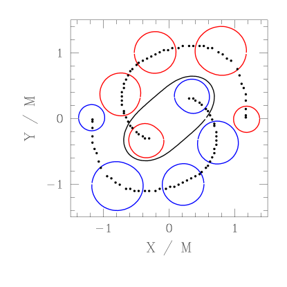
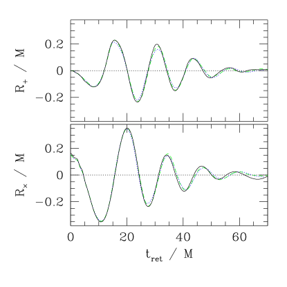
Figure 1: Numerical results for merger of binary BHs performed with the initial data of [18]. Left: The open thick circles denote evolution of the location of the apparent horizon of two BHs for $t/M=0$, 5, 10, 15, and 20 where $M$ is the total ADM mass at $t=0$. The open wide circle at $t=20M$ is the common apparent horizon. The small solid circles denote approximate location of the maximum of the conformal factor. The grid setting is $(N,N_{0},\Delta i,\xi,\Delta x/M_{p},L/\lambda)=$ (200,105,30,7,1/16,1.20) for this result (note that $\lambda\approx 37M$). Right: $+$ and $\times$ modes of gravitational waveforms extracted $r\approx\lambda$ for $(N,N_{0},\Delta i,\xi,\Delta x/M_{p},L/\lambda)=$ (200,105,30,9,0.05,1.20) (solid curves), (200,105,30,7,0.064,1.23) (dashed curves), and (200,105,30,5,0.08,1.23) (dotted curves).

For a test, we performed simulations for merger of two nonspinning BHs adopting the same initial condition as used in [18]. We focused particularly on the merger time, which is referred to as the time at which a common apparent horizon is first formed and found that it varies with improving grid resolution approximately at 1st order. The likely reason is that geometric variables vary steeply around the BH where they are evolved with 1st-order accuracy in our scheme, although other regions are resolved with 2nd-order accuracy. By the extrapolation, an exact merger time is estimated to be $\approx 19M$. This result agrees approximately with those of [18]. This indicates that our code can follow moving punctures (see the left panel of Fig. 1 for evolution of the location of apparent horizons for the initial condition of [18]).

Gravitational waves are also computed. In the right panel of Fig. 1, we display the results for three different grid resolutions. The figure shows that after merger, gravitational waves are determined by the quasinormal mode ringing and that the waveforms depend very weakly for chosen grid resolutions. The wavelength of the quasinormal mode is $\approx 11$–12M, which agrees with the result of [18].

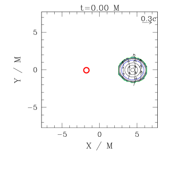
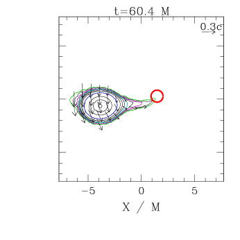
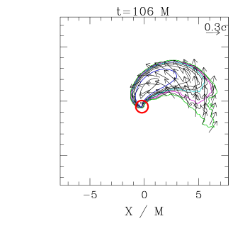
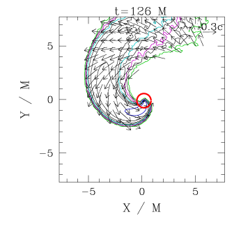
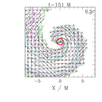
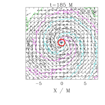
Figure 2: Snapshots of the density contour curves for $\rho$ in the equatorial plane for model A with $(N,N_{0},\Delta i,\xi,\Delta x/M_{p},L/\lambda)=$(220,150,9,3/40, 0.59). The solid contour curves are drawn for $\rho=(1+2i)\times 10^{14}~{}{\rm g/cm^{3}}~{}(i=1,2,3)$ and for $10^{14-0.5i}~{}{\rm g/cm^{3}}~{}(i=1\sim 8)$. The maximum density at $t=0$ is $\approx 7.2\times 10^{14}~{}{\rm g/cm^{3}}$. The blue, cyan, magenta, and green curves denote $10^{14}$, $10^{12}$, $10^{11}$, and $10^{10}~{}{\rm g/cm^{3}}$, respectively. Vectors indicate the velocity field $(v^{x},v^{y})$, and the scale is shown in the upper right-hand corner. The thick (red) circles are apparent horizons. Time is shown in units of total mass of the system $M$.

Next, we present the results for merger of BH and NS for model A. Figure 2 shows evolution of contour curves for $\rho$ and velocity vectors for $v^{i}$ in the equatorial plane together with the location of apparent horizons at selected time slices for $(N,N_{0},\Delta i,\xi,\Delta x/M_{p},L/\lambda)=$(220,150,9,3/40, 0.59). Due to gravitational radiation reaction, the orbital radius decreases and then the NS is elongated (2nd panel). Because of the elongation, the quadrupole moment of the NS is amplified and the attractive force between two objects is strengthen [35]. This effect accelerates an inward motion and, consequently, the NS starts plunging to the BH at $t\sim 90M$. Soon after this time, the NS is tidally disrupted; but the tidal disruption occurs near the ISCO and hence the material in the inner part is quickly swallowed into the BH (3rd and 4th panels). On the other hand, because of the outward angular momentum transfer, the material in the outer part of the NS forms a disk with the maximum density $\sim 10^{12}~{}{\rm g/cm^{3}}$ (5th and 6th panels).

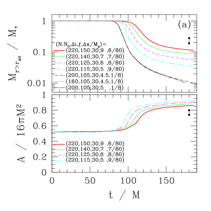
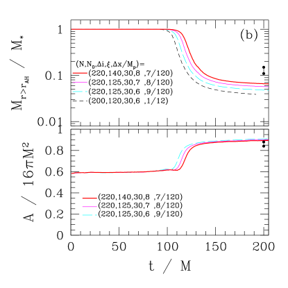
Figure 3: (a) Results for model A for various grid resolutions. Upper panel shows evolution of baryon rest-mass located outside the apparent horizon. The plots for $\Delta x=M_{\rm P}/8$ almost coincide and show that the results depend weakly on the values of $L$ and $\xi$. On the other hand, the results depend systematically on $\Delta x$ (see text). Lower panel shows evolution of area of apparent horizon in units of $16\pi M^{2}$. (b) The same as (a) but for model C.

Mass of the disk is not large. Figure 3(a) shows evolution of baryon rest-mass located outside apparent horizons $M_{r>r_{\rm AH}}$. We find that $\sim 80\%$ and $\sim 90\%$ of the mass is swallowed into the BH in $t\sim 130M\sim 2$ ms for models A and C, respectively, for the best grid-resolution simulations. The swallowing continues after this time. Note that since $M_{r>r_{\rm AH}}$ is rest-mass outside apparent horizons, the disk mass which should be defined for the mass located outside an ISCO around the formed BH is slightly smaller. We follow the evolution of the rest-mass of material located for $r>3M$ and $r>4.5M$, where $r=3M$–$4.5M$ are approximate locations of the ISCO around the formed BH, and find that their values are smaller than $M_{r>r_{\rm AH}}$ by $\sim 10\%$ and 20%, respectively. Thus, the disk mass would be 0.8–$0.9M_{r>r_{\rm AH}}$ in reality.

The value of $M_{r>r_{\rm AH}}$ depends systematically on $\Delta x$; we find that the results for good resolutions ($\Delta x/M_{p}=3/40$, 7/80, and 1/10 for model A and 7/120, 8/120, and 9/120 for model C) at late times approximately obey a relation of convergence, i.e., $M_{r>r_{\rm AH}}(t)=a(t)+b(t)\Delta x^{n}$ where $a(t)$ and $b(t)$ are functions of time. The order of convergence, denoted by $n$, is between 1st and 2nd order (i.e., $1<n<2$). For model A, least-square fitting gives $a(t)$ at $t=180M$ as $\approx 0.19M_{*}$ if we set $n=2$ and as $0.28M_{*}$ for $n=1$ (see the solid circle in Fig. 3(a)). For model C, they are $0.11M_{*}$ and $0.15M_{*}$ (the solid circle in Fig. 3(b)), respectively. Thus, the true result should be between $0.19M_{*}$ and $0.28M_{*}$ for model A and between $0.11M_{*}$ and $0.15M_{*}$ for model C.

It is reasonable that the disk mass for model C is smaller than for model A since the mass ratio of NS to BH is smaller for model C while the compactness of NS is nearly identical. A remarkable point is that with a small increase of the BH mass from $3.2M_{\odot}$ to $4.0M_{\odot}$, the disk mass decreases by a factor of 2. This suggests that the disk mass depends sensitively on the BH mass.

Note that the adopted NS has corotating velocity field initially and furthermore its radius is larger than that of canonical NSs. For irrotational velocity field with a realistic value of radius, the disk mass would be smaller than this value. It is reasonable to consider that our results for the disk mass provide an upper limit of the disk mass for given mass and spin of BH. Hence it is unlikely that a massive disk with $\sim M_{\odot}$ is formed after merger of nonspinning BH of mass $M>3M_{\odot}$ and canonical NS of mass $\approx 1.4M_{\odot}$ and radius $\approx 11$–13 km, although a disk of mass of $\sim 0.2$–$0.3M_{\odot}$ may be formed for small BH mass. This value of the disk mass is large enough to explain short GRBs of relatively low total energy $\sim 10^{49}$ ergs (e.g., [36] for an estimate).

Lower panels of Fig. 3 show the evolution of the area of apparent horizons in units of $16\pi M^{2}$. These illustrate that the area of BHs quickly increases swallowing material, and then, the area settles down to an approximate constant. We, again, evaluate the true final area by extrapolation for results with different grid resolutions. For model A, the area in units of $16\pi M^{2}$ at $t=180M$ is 0.74 and 0.80 in the assumption of the 1st ($n=1$) and 2nd-order ($n=2$) convergences, respectively (see the solid circles in Fig. 3(a)). For model C, $A/16\pi M^{2}$ at $t=200M$ is 0.84 and 0.88 for $n=1$ and $n=2$, respectively (see the solid circles in Fig. 3(b)). From these values the spin parameter of formed BHs, $a$, is approximately derived from

$${A\over 16\pi M_{\rm BHf}^{2}}={1+\sqrt{1-a^{2}}\over 2},$$ (19)

where $M_{\rm BHf}$ denotes the mass of the formed BH. To approximately estimate it, we simply use

$$M_{\rm BHf}=M-M_{r>r_{\rm AH}}-E_{\rm GW},$$ (20)

where $E_{\rm GW}$ is radiated energy by gravitational waves. We find that $E_{\rm GW}$ is about 1% of $M$ and simply use relation $E_{\rm GW}=0.01M$. Then we obtain $a=0.57$ and 0.52 for $n=1$ and 2 for model A and $a=0.52$ and 0.42 for $n=1$ and $n=2$ for model C. Thus, spinning BHs of moderate rotation are outcomes.

The spin parameter of the formed BHs is much smaller than the initial value of $J/M^{2}$ of the system. One of the reasons is that the disk has large angular momentum approximately written as $3M_{\rm BHf}M_{\rm disk}$ where $M_{\rm disk}$ denotes the disk mass $\sim 0.8$–$0.9M_{r>r_{\rm AH}}$ Here, the factor $3M_{\rm BHf}$ denotes a value of typical specific angular momentum around the formed BH. Denoting the initial angular momentum by $a_{0}M^{2}$ where $a_{0}\approx 0.73$ and 0.65 for models A and C (see Table I), the fraction of the angular momentum that the disk has is $\sim 3a_{0}^{-1}M_{\rm disk}M_{\rm BHf}/M^{2}$. Thus, for model A, the fraction is $\sim 20$–30% and for model C, it is 10–15%. In addition, gravitational waves carry away the angular momentum by $\sim 10\%$ of $a_{0}M^{2}$. Thus, the angular momentum of the formed BH should be smaller than the initial total angular momentum of the system by 30–40% for model A and by 20–25% for model C. Therefore, the values for $a$ derived above are reasonable magnitudes.

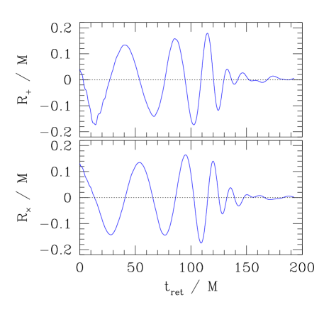
Figure 4: $+$ and $\times$ modes of gravitational waveforms for model C. $t_{\rm ret}$ and $M$ denotes the retarded time and the ADM mass of the system, respectively. The amplitude at a distance of observer can be found from Eq. (21).

In Fig. 4, gravitational waveforms for model C is shown. Gravitational waves are extracted from the metric near the outer boundaries using a gauge-invariant wave extraction method (see [16, 34] for details). From the values of $R_{+}$ and $R_{\times}$, the maximum amplitude of gravitational waves at a distance $D$ is evaluated

$$h_{\rm gw}\approx 10^{-22}\biggl{(}{\sqrt{R_{+}^{2}+R_{\times}^{2}}\over 0.31~{}{\rm km}}\biggr{)}\biggl{(}{100~{}{\rm Mpc}\over D}\biggr{)}.$$ (21)

Here, the maximum amplitude can be observed if the observer is located along the $z$-axis. Figure 4 implies that the maximum amplitude at a distance of $D=100$ Mpc is $\approx 5\times 10^{-22}$ since $M=5.26M_{\odot}$.

For $t_{\rm ret}\mathrel{\raise 1.29167pt\hbox{$<$}\mkern-14.0mu\lower 2.58334pt\hbox{$\sim$}}120M$, inspiral waveforms are seen: Amplitude increases and characteristic wavelength decreases with time. The wavelength at the final phase of the inspiral is $\sim 25M$ indicating that the orbital period of the ISCO is $\sim 50M$ (i.e., the angular velocity is $\sim 0.12M^{-1}$). This is in approximate agreement with the 3rd post-Newtonian results [31].

For $120M\mathrel{\raise 1.29167pt\hbox{$<$}\mkern-14.0mu\lower 2.58334pt\hbox{$\sim$}}t_{\rm ret}\mathrel{\raise 1.29167pt\hbox{$<$}\mkern-14.0mu\lower 2.58334pt\hbox{$\sim$}}150M$, ring-down waveforms are seen. The characteristic wavelength is $\sim 15M_{\rm BHf}$, which is in approximate agreement with the wavelength of the quasinormal mode.

The characteristic feature of gravitational waves after the merger sets in is that the amplitude damps quickly even in the formation of massive disk. This is due to the fact that the degree of nonaxisymmetry of the disk decreases in a very short time scale ($\sim 20$–$30M$). This indicates that in the frequency domain, the amplitude of Fourier power spectrum steeply decreases in the high-frequency region.

Figure 5: Evolution of averaged violation of the Hamiltonian constraint (a) for model A and (b) for C.

Figure 5 shows the evolution of averaged violation of the Hamiltonian constraint. For the average, rest-mass density is used as a weight (see [16] for definition) and the integral is performed for the region outside apparent horizons. The figure shows that the Hamiltonian constraint converges approximately at 2nd order. This result is consistent with the fact that the region except for the vicinity of BH is followed with 2nd-order accuracy.

5 Discussion

In this paper, we have presented our latest numerical results of fully GR simulation for merger of BH-NS binary, focusing on the case that the BH is not spinning initially and the mass ratio $q$ is fairly large as 0.3–0.4. It is found that even with such high values of $q$, the NS is tidally disrupted only for the orbit very close to ISCO and 80–90% of the mass element is quickly swallowed into the BH without forming massive disks. The results do not agree quantitatively with the prediction by the tidal approximation study. The reasons are: (1) In the tidal approximation, one describes NSs by the Newtonian gravity. In general relativity, gravity is stronger and the tidal disruption is less likely. (2) The time scale for angular momentum transfer during tidal disruption near the ISCO is nearly as long as the plunging time scale determined by gravitational radiation reaction and attractive force between two objects. Hence before the tidal disruption completes, most of the material is swallowed.

If the BH has a large spin, the final fate may be largely changed because of the presence of spin-orbit repulsive force. This force can weaken the attractive force between BH and NS and slow down the orbital velocity, resulting in smaller gravitational wave luminosity and longer radiation reaction time scale [37]. This effect may help massive disk formation. The study of spinning BH binaries is one of the next issues. The fate will also depend on EOS of NS [6] and mass of BH as well as on the velocity field of NS. Simulations with various EOSs and BH mass and with irrotational velocity field are also the next issues.

In this paper, a small number of the results for quasicircular states of BH-NS binaries are presented. Currently we are working in the computation of quasicircular states for a wide variety of masses of BH and NS in the framework described in Sec. 2. The numerical results will be reported in the near future [26].

Acknowledgements: MS thanks Y. Sekiguchi for useful discussion. Numerical computations were performed on the FACOM-VPP5000 at ADAC at NAOJ and on the NEC-SX8 at YITP in Kyoto University. This work was supported in part by Monbukagakusho Grants (No. 17540232) and by NSF grants PHY0071044, 0503366.

References

- [1] R. Narayan, B. Paczynski, and T. Piran, Astrophys. J. 395, 83 (1992).
- [2] R. Voss and T. M. Taulis, Mon. Not. R. Astro. Soc. 342, 1169 (2003); K. Belczynski, T. Bulik, and B. Rudak, Astrophys. J. 571, 394 (2002); V. Kalogera et al. Astrophys. J. 601, L179 (2004).
- [3] L. G. Fishbone, Astrophys. J. 185, 43 (1973); B. Mashhoon, Astrophys. J. 197, 705 (1975); J.-A. Marck, Proc. R. Soc. Lond. A 385, 431 (1983).
- [4] M. Shibata, Prog. Theor. Phys. 96, 917 (1996).
- [5] P. Wiggins and D. Lai, Astrophys. J. 532, 530 (2000).
- [6] M. Ishii, M. Shibata, and Y. Mino, Phys. Rev. D 71, 044017 (2005).
- [7] J. A. Faber, T. W. Baumgarte, S. L. Shapiro, K. Taniguchi, F. A. Rasio, Phys. Rev. D 73, 024012 (2006).
- [8] M. Vallisneri, Phys. Rev. Lett. 84, 3519 (2000).
- [9] L. Lindblom, Astrophys. J. 398, 569 (1992).
- [10] C. L. Fryer, S. E. Woosley, M. Herant, and M. B. Davies, Astrophys. J. 520, 650 (1999).
- [11] M. C. Miller, Astrophys. J. 626, L41 (2005).
- [12] W. H. Lee and W. Kluzniak, Astrophys. J. 526, 178 (1999); H. T. Janka, T. Eberl, M. Ruffert, and C. L. Fryer, Astrophys. J. 527, L39 (1999); S. Rosswog, astro-ph/0505007.
- [13] J. A. Faber, T. W. Baumgarte, S. L. Shapiro, and K. Taniguchi, Astrophys. J. 641, L93 (2006).
- [14] F. Löffler, L. Rezzolla, and M. Ansorg, gr-qc/0606104.
- [15] M. Shibata and K. Uryū, Phys. Rev. D submitted.
- [16] M. Shibata, K. Taniguchi, and K. Uryū, Phys. Rev. D 68, 084020 (2003).
- [17] M. Shibata, K. Taniguchi, and K. Uryū, Phys. Rev. D 71, 084021 (2005); M. Shibata and K. Taniguchi, ibid 73, 064027 (2006).
- [18] M. Campanelli, C. O. Lousto, P. Marronetti, and Y. Zlochower, Phys. Rev. Lett. 96, 111101 (2006); J. G. Baker, J. Centrella, D.-I. Choi, M. Koppitz, and J. van Meter, Phys. Rev. Lett. 96, 111102 (2006).
- [19] B. Brügmann, J. A. Conzalez, M. Hannam, S. Husa, and U. Sperhake, gr-qc/0610128.
- [20] M. Miller, gr-qc/0106017.
- [21] K. Taniguchi, T. W. Baumgarte, J. A. Faber, and S. L. Shapiro, Phys. Rev. D 72, 044008 (2006).
- [22] P. Grandclement, gr-qc/0609044 (2006).
- [23] K. Uryū, et al., Phys. Rev. Lett. 97, 171101 (2006).
- [24] S. Brandt and B. Brügmann, Phys. Rev. Lett. 78, 3606 (1997).
- [25] C. S. Kochanek, Astrophys. J. 398, 234 (1992); L. Bildsten and C. Cutler, ibid 400, 175 (1992).
- [26] K. Uryū and M. Shibata, in preparation.
- [27] J. R. Wilson and G. J. Mathews, Phys. Rev. Lett. 75, 4161 (1995).
- [28] M. D. Hannam, Phys. Rev. D 72, 044025 (2005).
- [29] P. Grandclement, E. Gourgoulhon, and S. Bonazzola, Phys. Rev. D 65, 044020 (2002); 044021 (2002). G. Cook, Phys. Rev. D 65, 084003 (2002).
- [30] M. Shibata, Prog. Theor. Phys. 101, 1199 (1999).
- [31] L. Blanchet, Living Rev. Relativ. Vol. 9, No. 4 (2006).
- [32] E.g., A. Akmal, V. R. Pandharipande, and D. G. Ravenhall, Phys. Rev. C 58, 1804 (1998): F. Douchin and P. Haensel, Astron. Astrophys. 380, 151 (2001).
- [33] M. Shibata and J. A. Font, Phys. Rev. D 72, 047501 (2005).
- [34] M. Shibata and T. Nakamura, Phys. Rev. D 52, 5428 (1995).
- [35] D. Lai, F. A. Rasio, and S. L. Shapiro, Astrophys. J. Supplement 88, 205 (1993).
- [36] S. Setiawan, M. Ruffert, and H.-Th. Janka, Mon. Not. R. astr. Soc. 352, 753 (2004); W. H. Lee, E. R. Ruiz, and D. Page, Astrophys. J. 632, 421 (2005).
- [37] E.g., L. Kidder, C. M. Will, and A. G. Wiseman, Phys. Rev. D 47, R4183 (1993).