The Evershed effect observed with 0$\farcs$2 angular resolution

Abstract

We present an analysis of the Evershed effect observed with a resolution of 0$\farcs$2. Using the new Swedish 1-m Solar Telescope and its Littrow spectrograph, we scan a significant part of a sunspot penumbra. Spectra of the non-magnetic line Fe i 7090.4 Å  allows us to measure Doppler shifts without magnetic contamination. The observed line profiles are asymmetric. The Doppler shift depends on the part of the line used for measuring, indicating that the velocity structure of penumbrae remains unresolved even with our angular resolution. The observed line profiles are properly reproduced if two components with velocities between zero and several  km s^-1 co-exist in the resolution elements. Using Doppler shifts at fixed line depths, we find a local correlation between upflows and bright structures, and downflows and dark structures. This association is not specific of the outer penumbra but it also occurs in the inner penumbra. The existence of such correlation was originally reported by Beckers & Schröter (1969), and it is suggestive of energy transport by convection in penumbrae.

1. Introduction

The spectral lines observed in sunspot penumbrae are both asymmetric and shifted in wavelength. This phenomenon, known as the Evershed effect, is commonly attributed to the presence of large and highly inclined plasma flows. Although the effect was discovered a hundred years ago (Evershed 1909) the true nature of these flows remains enigmatic, which hampers a full understanding of the penumbral physics. The observational properties of penumbrae and the Evershed effect are well covered in a number of recent review papers (e.g., Thomas & Weiss 1992, 2004; Solanki 2003), and we refer to them for an overview. This introduction is focused on a particular aspect of the effect directly connected to our observational work.

Penumbrae are almost as bright as the quiet Sun. Since the transfer of energy by radiation is inefficient, either the penumbrae are transparent and therefore very shallow, or the energy radiated away by penumbrae is transported from below by some sort of convective process Shallow penumbrae require nearly horizontal magnetic fields, which are not observed and which leaves us only the second option (Solanki & Schmidt 1993). Therefore, the penumbrae of sunspots, with their filaments and flows, are likely the result of convection taking place in highly inclined strong magnetic fields. However, there is no agreement on how the convection operates, i.e., on how the hot plasma rises, releases energy, and returns to the sub-photospheric layers, and how these motions occur in a strong magnetic field constraining the free movement of the plasma. Several possibilities have been put forward in the literature, and we will mention a number of them as example. The penumbrae may contain convective rolls, where the magnetic field lines are rigidly transported by the plasma motions, and which require very inclined magnetic fields (Danielson 1961). Depending on the magnetic field inclination, convection sets in as convective rolls or traveling waves (Hurlburt et al. 2000). Siphon flows along magnetic field lines have been proposed mainly for explaining the horizontal component of the Evershed flow (Meyer & Schmidt 1968; Thomas & Montesinos 1993; Weiss et al. 2004). However, such flows transport hot plasmas from the sub-photosphere, which become optically thin and radiate away internal energy. Individual magnetic fluxtubes that raise, cool off, and then fall represent another possibility. This process is called interchange convection by moving magnetic fluxtubes (Schmidt 1991; Jahn & Schmidt 1994), and it has been modeled in detail by Schlichenmaier et al. (1998a, b). A significant part of the convective energy transfer is not provided by the interchange motions, but by flows along field lines indirectly induced during the interchange (Schlichenmaier & Solanki 2003). In the vein of the thin penumbra models (Schmidt et al. 1986), but improved to get rid of the problems, Spruit & Scharmer (2006) propose the intrusions of non-magnetic convective cells.

None of the modes of convection mentioned above satisfy all the observational constraints and, simultaneously, none of the observations seem to be so deciding as to rule out particular models once and for all. The main problem probably lies in the insufficient spatial resolution of our observational description of the phenomenon. Convection could be easily identified upon detecting a clear correlation between vertical velocity and brightness, similar to that characteristic of the solar granulation. However, the flows in the penumbra are known to change direction and speed within scales smaller than the photon mean-free-path, a property inferred directly from observations (e.g., from the existence of broad-band circular polarization, Sánchez Almeida & Lites 1992; see also § 6). The photospheric mean-free-path length scale, some 150 km, is comparable with the angular resolution of the best images, therefore, even our best measurements are expected to average several structures with different physical properties. The observations always provide ill-defined averages of the measured properties, being each resolution element a volume of the solar photosphere. The size in the plane perpendicular to the line-of-sight (LOS) is set by the angular resolution, whereas the size along the LOS is set by the radiative transfer smearing (e.g., Sánchez Almeida 1998). Unscrambling the averages to retrieve properties of the unresolved structure is both difficult and prone to misinterpretations. Researchers have approached the problem assuming the existence of unresolved structures during the data analysis (e.g., Bumba 1960; Grigorjev & Katz 1972; Golovko 1974; Sánchez Almeida & Lites 1992; Solanki & Montavon 1993; Wiehr 1995; Sánchez Almeida et al. 1996; Westendorp Plaza et al. 2001; Bellot Rubio 2004; Sánchez Almeida 2005). Then the outcome of the analysis depends on the specific assumptions, a difficulty that increases as the resolution worsens and the observational average becomes coarser. On the contrary, improving the angular resolution removes part of the ambiguities and facilitates the interpretation of the observations. In view of past experiences, it is difficult to specify an observational plan that secures sorting out the penumbral puzzle. However, any successful plan necessarily requires improving the angular resolution to a point where the interpretation of the observations is not longer ambiguous.

The advent of the Swedish 1-m Solar Telescope (SST; Scharmer et al. 2003a, b) has opened up new possibilities since it routinely provides an angular resolution significantly better than its predecessors (Scharmer et al. 2002). We take advantage of the SST to carry out spectroscopic observations of the Evershed effect with an exceptional spatial resolution ($\simeq$0$\farcs$2; § 2). Our study is focused on the local correlation between brightness and Doppler shift originally found by Beckers & Schröter (1969) and later observed by others (Sánchez Almeida et al. 1993; Johannesson 1993; Schlichenmaier & Schmidt 1999; Schmidt & Schlichenmaier 2000). Features brighter than the local mean are associated with blueshift, and vice versa. The same correlation exist both in the limb-side penumbra and the center-side penumbra, a fact invoked by Beckers & Schröter (1969) to conclude that vertical motions rather than horizontal motions are responsible for the correlation. Such correlation between vertical velocity and intensity is characteristic of the granulation. The fact that the same correlation is also present in penumbrae suggests a common origin for the two phenomena, namely, convection. Despite the qualitative agreement, the amplitude of the velocity fluctuations, of the order of 100 m s^-1, is insufficient to transport the energy radiated away by penumbrae. Velocities similar to those of the non-magnetic granulation are required independently of the specific mode of convection responsible for the transport (see, e.g., Spruit 1987). We revisit the issue with the best resolution available at present to (a) confirm the existence of such correlation, and (b) see whether the improved resolution reveals vertical velocities large enough to account for the radiative losses of penumbrae. With this in mind, we seek independent support for various radically different observational studies suggesting the presence of convective motions in penumbrae. Filament like structures in velocity maps are found to join bright and dark knots (Schlichenmaier et al. 2004, 2005). A complex velocity pattern with small-scale upflows and downflows is able to reproduce the asymmetries of the Stokes profiles characteristic of penumbrae (Sánchez Almeida 2005). The same scenario is qualitatively consistent with the proper motions observed in a penumbra by Márquez et al. (2006b). The proper motions are predominantly radial but with a sideways component which arranges the plasma forming long narrow filaments co-spatial with dark features. Mass conservation arguments indicate that the accumulation of plasma in the dark filaments must be balanced by downflows of the order of 200 m s^-1.

Our study of the Evershed effect begins by describing the observations and the data reduction (§ 2 and Appendix A). The shape of the observed line bisectors is analyzed and discussed in § 3. The observed spectra show the correlation between Doppler shift and brightness discussed above. Its variation with the azimuth in the penumbra allows us to separate vertical and horizontal velocities (§ 4). Line asymmetries are analyzed in § 5 in terms of two spatially unresolved components. The implications of our work for understanding the structure of penumbrae are discussed in § 6, where we also consider consistencies and inconsistencies with previous studies. Finally, Appendix B shows that the kind of weak correlation between vertical motions and brightness found in penumbra is also observed in the quiet Sun when the spatial resolution is insufficient to resolve individual granules.

2. Observations and data reduction

The observations were carried out on October 16, 2004, using the SST equipped with AO and a Littrow spectrograph (Scharmer et al. 2003a, b; Kiselman et al. 2006, ). We obtained spectrograms of the non-magnetic line Fe i 7090.4 Å in the penumbra of the decaying circular sunspot NOAA 10682 (heliocentric angle $\theta\simeq 35^{\circ}$; $\cos\theta$=0.82). The black rectangular box in Figure 1 indicates the field-of-view (FOV).

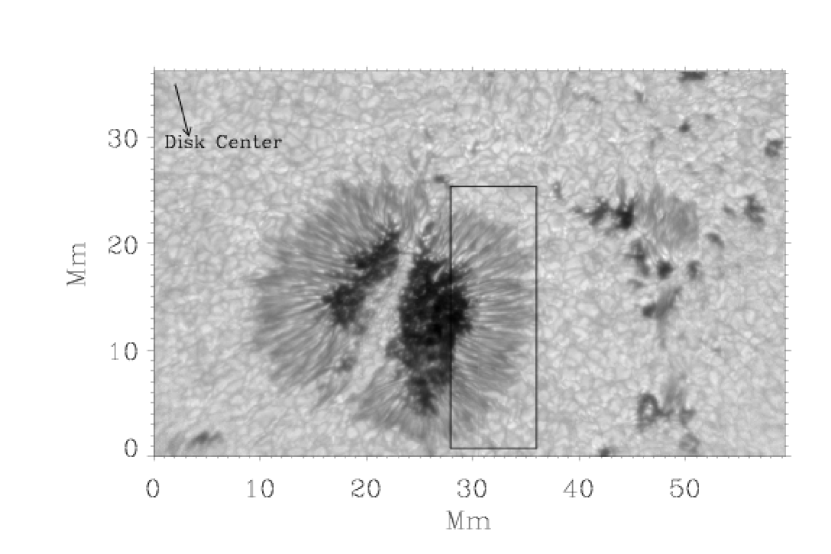
Figure 1.— Slit-jaw of one of the exposures showing our field of view (the box). The axes are given in Mm from the lower left corner, and an arrow points out the direction of the solar disk center. The scan was carried out from left to right with the slit in the vertical direction. (The slit was artificially removed from this slit-jaw image during the flatfielding procedure.) The image was obtained with a 7 Å wide color filter centered in 7057 Å.

We employ a non-magnetic line to avoid contaminating the inferred velocity fields with cross-talks coming from the penumbral magnetic field. The penumbra was scanned from the inner to the outer boundaries with steps of 0$\farcs$12 perpendicular to the slit. The slit width was set to 0$\farcs$11, which corresponds to 29 mÅ in the focal plane of the spectrograph and sets the spectral resolution of the data. Given the pixel size of the camera and the effective focal length at the focal plane of the spectrograph, the sampling interval of the spectra is 0$\farcs$04 along the slit and 10.5 mÅ across the slit, which suffices for the spatial and spectral resolution of the data. We use frame selection triggered by the spectrograph camera, providing the four spectra of highest contrast every 20.8 s. The exposure time was set to 150 ms. The scan covers an effective FOV of 10$\farcs$5 (across the slit) $\times$ 34$\farcs$4 (along the slit), and it required 31 min to be completed. Together with the spectrograms, we gather simultaneous slit-jaw and Ca H images (an example of the former is shown in Fig. 1). They were used to set up the polar coordinate system used for the analysis of velocities carried out in § 4, which requires identifying the direction of the solar disk center, as well as assigning a curvature radius and a curvature center to the penumbra. The data are corrected for dark current and flatfield using standard procedures. In addition, we correct the spectra for the Modulation Transfer Function (MTF) characteristic of an ideal 1-m telescope at the working wavelength. Since the penumbral structures are predominantly elongated across the slit, the deconvolution process can be reduced to a 1D problem using as MTF a radial cut across the 2D axi-symmetric MTF of a diffraction limited telescope (see, e.g., Sánchez Almeida & Bonet 1998). The deconvolution, including optimum filtering, is carried out in the Fourier domain following the procedure explained in detail by Sobotka et al. (1993).

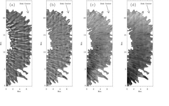
Figure 2.— (a) Map of continuum intensity. (b) Doppler shift of the bisector at 80% of the line depth. Running means have been subtracted in these two maps to bring out only local variations. (c) Difference between the Doppler shifts of the bisectors at 80% and 20% without running mean subtracted. Images (b) and (c) share the same scale of grays which goes from -2 km s^-1(black) to +2 km s^-1(white). (d) Original map of the Doppler shift without the running mean subtracted and represented with a scale spanning from -4 km s^-1(black) to +4 km s^-1(white). According to our convention, redshifts correspond to positive Doppler shifts. The centers of the symbols in (a) indicate the positions of the representative line profiles shown in Figure 4.

From the best spectrogram per slit position, we construct the 2D continuum image of the FOV shown in Figure 2a. Each column corresponds to one slit position so that the full set provides an image. Residual image motion in the direction parallel to the slit has been removed from the image by cross-correlation techniques. We shift the different columns so that the cross-correlation between adjacent columns is maximum. The same small re-arrange of the columns inferred from the continuum intensity is applied to all the maps displayed and discussed in the paper. This manipulation was carried out mainly for aesthetic reasons, since the residual image motion has very limited impact on the results of our analysis, which is based on correlations between parameters obtained in the same pixels. The angular resolution of our spectra turns out to be very close to 0$\farcs$2, as inferred from the cutoff frequency of the power spectra of continuum fluctuations in the spatial direction of the spectrograms. Figure 3a shows the power spectrum for the variations of intensity along the slit. We average the power spectrum of all the columns forming the continuum image in Figure 2a. Both the original spectra and the MTF reconstructed spectra show signals above the noise at 5 arcsec^-1, corresponding to a scale of 0$\farcs$2. The same conclusion can be drawn from Gaussian fits to the narrowest continuum features in the spectra. Figure 3b shows one of these features reproduced with a Gaussian having a FWHM of 0$\farcs$19.

Figure 3.— (a) Power spectrum for the intensity variations along the slit. The dotted line shows the average among all our penumbral spectra before restoration. The solid line represents the same average after restoration. The horizontal dotted line corresponds to the level of power at the cutoff imposed by the telescope diameter and, therefore, it indicates the level of noise. There is power in the original unprocessed image even beyond 5 arcsec^-1, corresponding to a scale of 0$\farcs$2. The restoration includes a noise filter that damps down the spectrum starting at this threshold. (b) The solid line shows observations of the intensity variation across a representative narrow structure in one of the spectra. The symbols correspond to a least squares fit of this profile with a Gaussian plus a parabolic background, the latter represented by the dashed line. The Gaussian has 0$\farcs$19 FWHM, indicating that features of this width can be resolved in our spectra.

The work aims at analyzing absolute Doppler shifts, which requires a careful calibration of the wavelength scale. First, the relative wavelength scale along the spectrograph slit was set using spectrograms taken while the telescope pointing was moving across the solar disk. The spectral line must have the same wavelength in these flatfield images, an information used to bring to a common scale all the spectra taken in each position of the scan. As we argue below, the spectrograph was stable enough during the scan to allow a direct comparison of the wavelengths taken at different positions, which provides a consistent relative wavelength scale for the whole scan. Therefore, one can set a common absolute scale by knowing the absolute wavelength of only one spectrum. We set such scale assigning zero velocity to the mean line shift obtained from the minimum of Fe i 7090.4 Å in the darkest parts of the umbra. According to Beckers (1977), such absolute velocity is uncertain by less than 100 m s^-1. Umbral oscillations may have an influence on the velocity scale thus obtained, but their amplitudes are again smaller than 100 m s^-1 (e.g., Lites 1992). The effect of the spatial stray-light is analyzed in Appendix A, and it turns out to be negligible. We can assure the stability of the spectrograph during the scan because of the position the H₂O telluric line at 7094.05 Å. The wavelength of the minimum of this line in the absolute scale used for Fe i 7090.4 Å is constant with a rms fluctuation of only 90 m s^-1. Most of these fluctuations result from uncertainties in determining the minima of the weak telluric line (equivalent width of only 5 mÅ). In short, our absolute wavelength scale provides velocities with an accuracy of the order of 100 m s^-1.

3. Bisectors and unresolved velocities

Spectral lines formed in atmospheres of constant velocity are symmetric and shifted as a whole, therefore, one should get the same Doppler shift independently of the part of the line used for measuring. Since this is not the case of our penumbral spectra, we conclude that even with 0$\farcs$2 angular resolution a significant part of the penumbral velocity structure remains unresolved. We bring up this fact by computing the bisectors of the intensity profiles. The bisector of an intensity profile is the line joining the mid points of the profile at each intensity level. (The intensity level is usually quantified using a percentage, with 0% representing the line core and 100% the continuum.) Figure 4 shows a few representative examples of observed line profiles and bisectors.

Figure 4.— Representative line profiles showing large asymmetries and the corresponding bisectors. Top: profiles of bright features. Bottom: profiles of dark features. Left: profiles on the limb-side penumbra. Right: profiles on the center-side penumbra. The actual positions are indicated by the symbols in Figure 2a. Wavelengths are in km s^-1 in our absolute velocity scale, whereas the intensities are given in units of the mean quiet Sun continuum intensity.

The bisector must be a vertical straight line if the atmosphere has a constant velocity, however, the bisectors of Fe i 7090.4 Å are curved and inclined. They show different velocities at different line depths, indicating that the velocity structure is finner than our resolution. The lack of enough resolution is not an exception attributable to a few pixels. Figure. 2c shows a map of the velocity difference between the bisector at line wings (80%) and the bisector at line core (20%). The map of differences follows a pattern with the characteristic filamentary appearance of the penumbra. The typical values differ from zero, and values as large as one km s^-1 are not unusual. The dispersion of velocities responsible for these bisectors must be large, a conclusion that we try to quantify with the two-Gaussian fits presented in § 5.

As it is pointed out in § 1, our resolution element is actually a volume, with the size in the plane perpendicular to the LOS set by the angular resolution, and the size along the LOS set by radiative transfer smearing. Consequently, observing slanted bisectors do not allow us to know if the gradients of velocity occur along or across the LOS. The two of them probably coexist (see § 6).

4. Relationship Between Continuum Intensity and Velocity

In agreement with Beckers & Schröter (1969) and others (e.g. Sánchez Almeida et al. 1993; Johannesson 1993; Schmidt & Schlichenmaier 2000, see § 1), we find a local correlation between continuum intensity $I$ and Doppler shift $U_{D}$. The purpose of the section is twofold. First, it describes the observed correlation. Second, horizontal and vertical motions are separated to show that a significant part of the correlation is due to vertical motions.

The local variations are obtained by subtracting from the original maps a running mean. Figure 2b has been computed from the original Figure 2d using a running box 1$\farcs$6 wide. The same box is used for the intensity in Figure 2a. We also tried with boxes half and twice this value to conclude that the actual width is not critical (see below). The correlation can be observed directly from inspection of the velocity and intensity images, e.g., Figure 5.

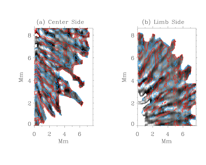
Figure 5.— Continuum images of a portion of the center-side penumbra (a) and the limb-side penumbra (b) overlaid with contours of the velocity field inferred from bisector shifts at line wings (Fig. 2). Both the intensities and the velocities represent local variations; the large scale variation has been removed by subtracting a smoothed version of the original maps. Blue and red contours correspond to blueshifts and redshifts, respectively ($\pm$250 m s^-1). The velocity contours show a clear filamentary structure. Note that blueshifts tend to be associated with bright features, and vice-versa. It is not a one-to-one correlation, though. Such association is more pronounced in the limb-side penumbra, but it is also present in the center-side penumbra, indicating that it must be produced by vertical rather than horizontal velocities.

It shows how local blueshifts are preferentially associated with local bright features. The correlation is more clear in the limb-side penumbra (Fig. 5b), but it is also present with the same sign in the center-side penumbra (Fig. 5a). The relationship can be quantified as,

$$U_{D}-\langle U_{D}\rangle\simeq m~{}(I-\langle I\rangle)+k,$$ (1)

with the angle brackets denoting local running mean averages. In this equation and throughout the paper the intensity $I$ is referred to the quiet Sun continuum intensity and therefore is a dimensionless parameter, whereas the sign of $U_{D}$ is chosen to be positive for redshifts.

Figure 6 shows the observed variation of the Doppler shift versus continuum intensity for two sections of our FOV, one in the limb-side penumbra (a) and the other in the center-side penumbra (b). We represent the mean Doppler shift considering intensity bins of $0.01$. The slope $m$ varies within the sunspot, from the center-side penumbra to the limb-side penumbra. However, it maintains a negative sign implying that bright features are associated with blueshifts (Fig. 6). The fact that $m$ keeps the sign implies that the correlation is produced by vertical motions, since the line-of-sight component of the horizontal radial velocities changes sign from the center-side penumbra to the limb-side penumbra (Beckers & Schröter 1969).

Figure 6.— Doppler velocity versus continuum intensity in sectors at the limb-side penumbra (a) and the center-side penumbra (b). The symbols and the solid lines correspond to observations and linear fits, respectively. The error bars represent standard deviations of the mean Doppler shift considering all the points with a given intensity $I-\langle I\rangle$. Velocities are measured from bisectors at line wings (Fig. 2b).

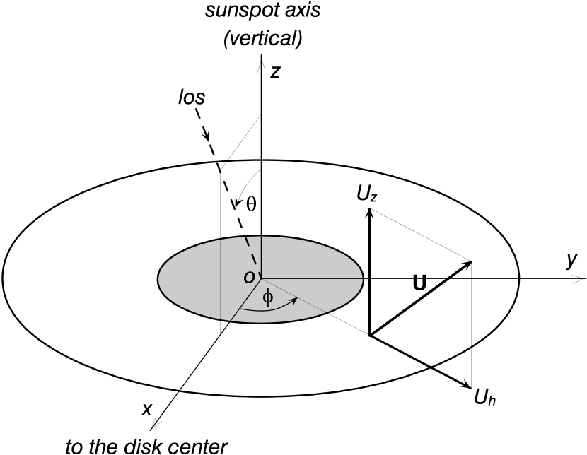
Figure 7.— Schematic with a sunspot and the reference system used to define angles and velocities. The line-of-sight (LOS) corresponding to the heliocentric angle of observation $\theta$ is shown as a dashed line. The velocity U of a point on the penumbra with an azimuth $\phi$ only has a vertical component $U_{z}$ and a radial horizontal component $U_{h}$. The sunspot axis coincides with the solar vertical direction, and the line joining the sunspot axis and the solar disk center sets the origin of $\phi$.

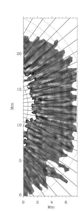
Figure 8.— Image of the FOV with the grid used to assign to the spectra polar coordinates centered on the sunspot umbra.

Figure 9.— Slope of the relationship between intensity and Doppler shift $m(\phi)$ versus the cosine of the azimuthal angle within the sunspot $\phi$. The error bars are formal error bars obtained from the fit used to derive $m(\phi)$.

This qualitative argument can be quantified adopting the following model for the relationship between velocities and intensities,

$$U_{z}= m_{z}\,(I-\langle I\rangle)+k_{z},$$ (2)

$$U_{h}= m_{h}\,(I-\langle I\rangle)+k_{h},$$ (3)

where $m_{z}$, $k_{z}$, $m_{h}$ and $k_{h}$ are constants, and $U_{z}$ and $U_{h}$ represent the vertical and horizontal velocities in the absolute reference system portrayed in Figure 7. ($U_{z}>0$ for upward velocities and $U_{h}>0$ for outward velocities.) If the motions are predominately radial so that the azimuthal component can be neglected,

$$U_{D}=-(U_{h}\,\sin\theta\,\cos\phi+U_{z}\,\cos\theta),$$ (4)

with the symbol $\theta$ representing the heliocentric angle of observation (Maltby 1964; Schröter 1967). This model leads to equation (1) with the slope $m$,

$$m(\phi)=-(m_{h}\,\sin\theta\,\cos\phi+m_{z}\,\cos\theta),$$ (5)

and with the running mean average Doppler shift,

$$\langle U_{D}\rangle=-(k_{h}\,\sin\theta\,\cos\phi+k_{z}\,\cos\theta).$$ (6)

The average Doppler shifts and slopes depend on the azimuth $\phi$. In order to apply the model to the observed velocities, we construct a polar coordinate system that assigns azimuths and radial distances to each position of the FOV. The center of curvature of the observed penumbra was estimated visually by trial-and-error so that the grid of polar coordinates provides radii parallel to the observed penumbral filaments. The best compromise is shown in Figure 8. The direction of the solar disk center sets the origin of the azimuths and it was obtained by comparison of the slit-jaw images with quasi-simultaneous full disk MDI continuum images. Figure 9 shows $m(\phi)$ obtained within the sectors of approximately constant azimuth in Figure  8 when the Doppler shifts in Figure 2b are used (bisector shift at line wings). Figures 6a and 6b illustrate the kind of fit leading to $m(\phi)$. Using the model in equation (5), a linear fit $m(\phi)$ versus $\cos\phi$ renders,

$$m_{z}\simeq ~{}(3.3\pm 0.4)~{}{\rm km\,s}^{-1},$$ (7)

$$m_{h}\simeq (-3.7\pm 0.8)~{}{\rm km\,s}^{-1}.$$ (8)

The error bars are 1-sigma formal errors provided by the least-squares routine, and assume that the deviations of the data from the fitted line are due to random noise (see Fig. 9). The sign $m_{h}<0$ indicates that horizontal velocities are enhanced in dark features, whereas $m_{z}>0$ implies that upflows occur in bright features. The fact that $m_{h}<0$ and $m_{z}>0$ is a firm result, as it is indicated by the error bars. We also checked that bisectors at different line depths can be used to compute velocities without modifying the resulting signs. The use of bisectors closer to the line core only reduces the amplitude of the velocities. We also repeated the calculations using only the inner half of the penumbra, i.e., the half closest to the umbra. The signs of $m_{z}$ and $m_{h}$ are not modified. In addition, we carried out the whole analysis doubling and halving the width of the box used to compute the running mean. Again the signs of $m_{z}$ and $m_{h}$ remain. Decreasing the width reduces the amplitude of the correlation whereas increasing the width has almost no effect on $m_{z}$ and $m_{h}$.

With the same approach leading to $m_{z}$ and $m_{h}$, one can use the local average Doppler shifts $\langle U_{D}\rangle$ to infer the constants $k_{z}$ and $k_{h}$ (see equation [6]). It renders,

$$k_{z}= (-0.48\pm 0.05)~{}{\rm km\,s}^{-1}$$ (9)

$$k_{h}= (3.30\pm 0.15)~{}{\rm km\,s}^{-1},$$ (10)

where the error bars are also formal errors from the linear least-squares fit. The finding of downward velocities in penumbrae ($k_{z}<0$) is not new. Downward velocities have been measured by many observers starting with the work by Rimmele(1995; see also Servajean 1961). These downward motions tend to be localized in the external parts of the penumbra, but the actual distribution depends on the specific measurement. Figure 10a shows several among the published values (Rimmele 1995; Schlichenmaier & Schmidt 2000; Tritschler et al. 2004; Sánchez Cuberes et al. 2005), which are presented as vertical velocity versus distance to the sunspot center. In order to compare our result with them, we consider that $k_{z}$ and $k_{h}$ in equation (3) depend on the radial distance to the sunspot center $\rho$. Our penumbra is divided in bands of constant radial distance (Fig. 8). Then equation (6) was fitted to the azimuthal variation of the running mean Doppler shift in each one of these bands, which renders $k_{z}(\rho)$ and $k_{h}(\rho)$. The results have been represented in Figure 10; the solid lines with symbols, with the symbols indicating the center of the band used to carry out the fits. We find mild upflows in the inner penumbra and downflows in the outer penumbra. These features are common to almost all the other measurements portrayed in Figure 10a. The mean horizontal velocities reach values of up to 3.7 km s^-1 not far from the external penumbral border, in agreement with values reported in the literature (Fig. 10b). Our curves remain within the scatter of the published values, a fact pointed out to argue that no obvious error burdens the validity of our velocity scale. The quantitative differences between the curves represented in Figure 10 can be attributed to many factors biasing this type of observation, e.g., variations from sunspot to sunspot, different systematic errors in the absolute velocity scales, the use of different spectral lines and procedures to infer velocities, the different ways of estimating sunspot radii, etc. Although the vertical velocities that we find are somehow larger than previous estimates (Fig. 10a), the values are close to those reported by Rimmele (1995) and Sánchez Cuberes et al. (2005), which correspond to sunspots observed at the very solar disk center, so that the Doppler shift directly yields vertical velocities without geometrical transformations. In the particular case of Sánchez Cuberes et al. (2005), they carry out a 1D inversion of the spectra to interpret the observed line asymmetries. Consequently, they obtain a velocity for each optical depth along the LOS. We represent the velocity at the bottom of the atmosphere (continuum optical depth equals 0.3), where the line-wings are formed.

We would like to stress that interpreting the average vertical velocities shown in Figure 10a is not trivial. They have been inferred as systematic Doppler shifts of the observed spectral lines (the part of the Doppler shift independent of $\cos\phi$; see equation [6]). According to Sánchez Almeida (2005), these net Doppler shifts may not necessarily represent net vertical plasma motions. If the penumbrae have plasma moving up and down, and if the thermodynamic conditions of these upflows and downflows are not identical, then there will be a net displacement of the average spectrum even though there is no net plasma motion. This lack of cancellation of the net signal is responsible for the well known convective blueshift of the spectral lines observed in the quiet Sun (e.g. Dravins et al. 1981).

Figure 10.— (a) Variation of $k_{z}$ with the distance to the sunspot center (the solid line with symbols). Note the tendency for $k_{z}$ to be negative. It is not very different from other Doppler shifts reported in the literature and also included in the plot. The symbols in the inset stand for Schlichenmaier & Schmidt (2000) (S&S 00), Rimmele (1995) (R 95), Tritschler et al. (2004) (T et al 04), and Sánchez Cuberes et al. (2005) (SC et al 05). (b) Variation of $k_{h}$ with the distance to the sunspot center. All radial distances are referred to the sunspot radius $R_{s}$ ($\simeq$14 Mm).

5. Two-Gaussian fit

We also studied whether the observed line asymmetries can be reproduced by means of two spatially unresolved velocity components. Bumba (1960) puts forward the idea, and it has been pursued by many others ever since (e.g., Maltby 1964; Stellmacher & Wiehr 1971; Wiehr 1995; Ichimoto 1988). We fit the line profiles $S(\lambda)$ with two Gaussian functions plus a continuum,

$$S(\lambda)= S_{c}(\lambda)-d_{1}\,\exp\big{\{}-{1\over 2}[(\lambda-\lambda_{1})/\sigma_{1}]^{2}\big{\}}$$

$$-d_{2}\,\exp\big{\{}-{1\over 2}[(\lambda-\lambda_{2})/\sigma_{2}]^{2}\big{\}},$$

with the continuum given by,

$$S_{c}(\lambda)=a_{0}+\lambda\ a_{1}+\lambda^{2}\ a_{2},$$ (12)

and symbols $\lambda_{i},\sigma_{i}$ and $d_{i}$ representing, respectively, the central wavelength, the width, and the depth of the two Gaussians ($i=1,2$). The fits are in general very good, like the examples shown in Figure 11. Note how the symbols used to represent the observations cannot be distinguished from the dotted line representing the fits, meaning that the two Gaussians are able to reproduce the asymmetries of the observed line profiles.

Figure 11.— Examples of two-Gaussian fits. Top: limb-side profile. Middle: center-side profile. Bottom: umbra-penumbra border profile. The symbols represent the observations whereas the dotted line shows the fits. The solid lines correspond to the two Gaussians used in the fit. The continuum has been added to the individual Gaussians to facilitate comparison.

The two components have very different Doppler shifts (i.e., different $\lambda_{i}$). The components in each pixel have been classified either as shifted or as unshifted depending on which one has the largest absolute Doppler shift. As it is shown in Figure 12, the unshifted component has almost no velocity throughout the penumbra, whereas the shifted component follows the pattern characteristic of the Evershed effect, with blueshifts in the center-side penumbra and redshifts in the limb-side penumbra.

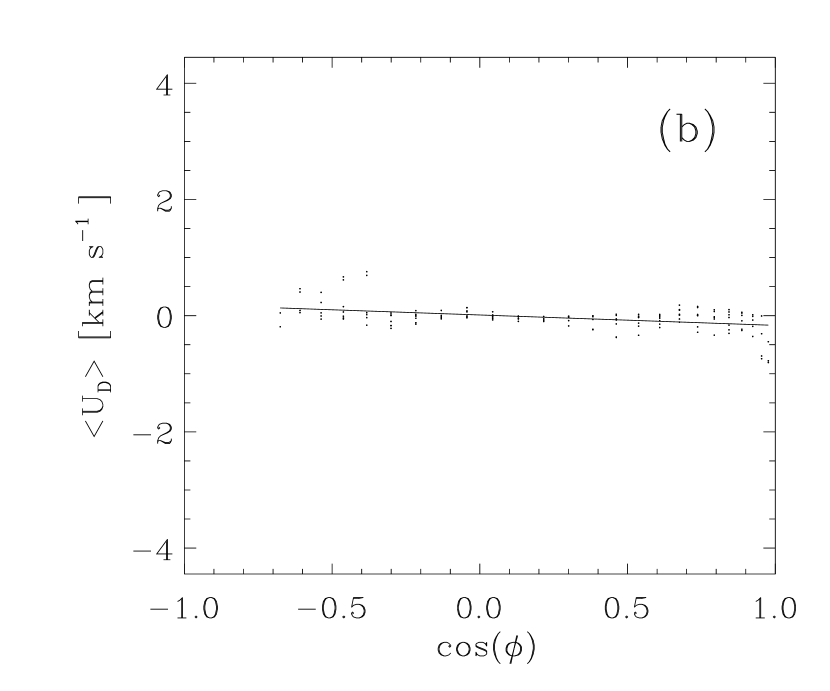
Figure 12.— Mean Doppler shift versus cosine of the azimuthal angle for the two Gaussian components that reproduce the line asymmetries. (a) Shifted component. It shows the pattern characteristic of the Evershed flow, with blueshifts in the center-side penumbra ($\cos\phi\simeq 1$) and redshifts in the limb-side penumbra ($\cos\phi\simeq-1$). (b) Unshifted component, showing very small Doppler shifts. Each point represents the average Doppler shift over a small range of azimuths and radial distances (the sectors represented in Fig. 8). Error bars are not included to avoid overcrowding, but they are smaller than the scatter among individual points.

The velocities of the shifted component are larger than those inferred from the bisectors.

The two components contribute similarly to the line profiles, except in the inner penumbra, where the unshifted component dominates. An example of two-Gaussian fit in the innermost penumbra is shown in Figure 11, bottom. Note the broad and shallow shifted component, and how the unshifted component dominates the line profile. Figure 13 illustrates the same result in a more systematic way. We use the equivalent width to parameterize the strength of the component. The equivalent width $W$ is defined as the area above the line profile normalized to the continuum intensity. In the case of Gaussian profiles,

$$W_{i}\simeq\sqrt{2\pi}\,d_{i}\,\sigma_{i}/S_{c}(\lambda_{c}),$$ (13)

where we have neglected the variation of the continuum within the line profile so that the continuum intensity $S_{c}(\lambda)\simeq S_{c}(\lambda_{c})$, with $\lambda_{c}$ the line core wavelength. Figure 13 shows the excess of equivalent width of the two components as a function of the distance to the sunspot center. Following the approach of the previous sections, we remove a running mean local average to show local variations. We subtract $\langle W\rangle/2$ with $\langle W\rangle=\langle W_{1}\rangle+\langle W_{2}\rangle$. This local mean is the same for the two components to ensure that the differences do not come from the two components having different local means. Figure 13 shows how the unshifted component tends to have an equivalent width significantly larger than the shifted component for $\rho<0.65\,R_{s}$, whereas the contribution of the two components balances from this radius on. (The symbol $R_{s}$ stands for radius of the sunspot.) Actually, the shifted component shows a small excess at 0.75, and then the unshifted component takes over again.

Figure 13.— Radial variation of the equivalent widths of the shifted component (the dashed line) and the unshifted component (the dotted line). The same local mean equivalent width has been subtracted from the two components.

The unshifted component seems to be brighter since it dominates in the bright pixels. Figure 14 shows how the equivalent widths of the two components vary with the local intensity. The equivalent width of the unshifted component is larger in the bright pixels ($I>\langle I\rangle$), whereas the contribution of the two components balance in the locally dark features ($I<\langle I\rangle$).

Figure 14.— Equivalent width of the shifted component (the dashed line) and the unshifted component (the dotted line). The unshifted component dominates in locally bright structures, suggesting an association between bright features and the unshifted component. The error bars represent the standard deviation of the averages represented in the figure.

As we point out above, the Doppler shifts of the shifted component resembles but exceeds the Doppler shifts derived from the bisectors. The corresponding mean vertical and horizontal velocities can be inferred following the same approach employed for the velocities based on bisectors. Figure 15 shows $k_{z}$ and $k_{h}$ obtained from a least squares fit of the Doppler shifts of the two components using equation (6). Points grouped by radial distance are used to obtain the radial variation. (The same approach used to derive Fig. 10.)

Figure 15.— (a) Vertical velocities $k_{z}$ and (b) horizontal velocities $k_{h}$ for the two components resulting from the two-Gaussian fits of the asymmetric line profiles. We also include the velocities inferred from the bisector analysis for reference (the solid line with symbols, as in Fig. 10.) The unshifted component presents very small velocities. Systematic horizontal velocities of up to 5 km s^-1 characterize the shifted component (the dashed line). This component also shows upflows in the inner penumbra ($k_{z}>0$ for $\rho/R_{s}<0.7$) and downflows in the external penumbra.

The shifted component shows systematic horizontal velocities of up to 5 km s^-1, and it presents moderate upflows in the inner penumbra ($k_{z}<0.5$ km s^-1) and larger downflows in the outer penumbra ($k_{z}\simeq 1.5$ km s^-1). Simultaneously, the unshifted component shows velocities never exceeding 1 km s^-1. Because of the quality of the fits, one can conclude that reproducing the observed bisectors requires plasmas with velocity amplitudes between 0 and 5 km s^-1 coexisting in our 0$\farcs$2 resolution elements. In the case of the shifted component the upflows in the inner penumbra exceed our observational uncertainties ($\sim$100 m s^-1; see § 2). However, we are reluctant to interpret these shifts as systematic upflows present in the inner penumbra. If the properties of the shifted component are taken literally, they indicate the existence of spatially unresolved upflows and downflows of the order of several km s^-1, a feature that is more meaningful that the small systematic upflow. The upflow may be real, but it may also be a false residual left if the Doppler signals of the large upflows and downflows are not strictly proportional to the flow of mass. The existence of such large upflows and downflows follows from the analysis of Figure 16, which shows the variation with the radial distance of the widths of the two Gaussian components ($\sigma_{1}$ and $\sigma_{2}$ in equation [5]). The width of the shifted component reaches a value of up to 5 km s^-1 in the inner penumbra, and this value is almost independent of the azimuthal angle within the sunspot. This width is too large to be due to thermal motions ($\sim$ 1 km s^-1 for penumbral temperatures of 5500 K), and it is also much larger than the typical widths of the profile of Fe i 7090.4 Å ($\sim$2 km s^-1 in the quiet Sun). Then if the inferred widths are due to spatially unresolved motions, it means that redward and blueward velocities of several km per second are associated with the shifted component in the inner penumbra. Since the widths do not depend on the azimuthal angle within the sunspot, such large velocity dispersion is also representative of the vertical velocities and, consequently, upflows and downflows of several km per second are associated with the shifted component. According to Figure 16, the width of the shifted component suffers a strong decrease from the inner to the outer penumbra. Observations have consistently shown that the widths of the spectral lines increase from the inner to the outer penumbra (e.g., Johannesson 1993; Rimmele 1995; Tritschler et al. 2004), which seems to be at variance with our result. However, there is no obvious inconsistency keeping in mind that the shifted component does not contribute to the line profile in the inner penumbra (Fig. 13). The profile is dominated by the unshifted component, which is very narrow and whose width increases with the radial distance (Fig. 16). Consequently, the line width of the full profile is expected to go from the values of the unshifted component in the inner penumbra, to some kind of average between the widths of the two components in the outer penumbra, thus increasing from the inner to the outer penumbra (see Fig. 16).

A final caveat is in order. Like the use of bisectors, the two-Gaussian fit is only an heuristic representation of the observed line asymmetries. The two components resulting from our fits do not necessarily represent two physical components existing in the penumbra, and a literal interpretation of the properties of the components may be misleading. The Evershed effect is not only the result of combining two separate components. This description is incomplete since two unresolved but symmetric components cannot account for the broad-band circular polarization observed in sunspots (see § 6).

Figure 16.— Variation with the radial distance of the widths of the two Gaussian components. They are given in km s^-1 versus radial distance normalized the Sunspot radius $R_{s}$. The dotted line corresponds to the unshifted component whereas the dashed line represents the shifted component. (A Gaussian has a FWHM some 2.35 times the parameter $\sigma_{i}$ represented in the figure.)

6. Discussion and Conclusions

We find local upflows associated with bright structures and local downflows associated with dark structures in 0$\farcs$2 angular resolution spectra (§ 4). The correlation keeps the same sign in the limb-side penumbra and the center-side penumbra, which indicates that it is due to vertical motions. The correlation remains even when only the inner half of the penumbra is considered. The existence of such correlation was originally reported by Beckers & Schröter (1969), and it is suggestive of convective motions in penumbrae. It has the sign required to transport energy by convection, although the magnitude of the inferred velocities is not yet enough to account for the observed radiative flux (see the discussion below). This deficit could be caused by the still insufficient spatial resolution of the present data. Appendix B shows how the correlation in penumbrae is qualitatively similar to the intensity velocity relationship found in the quiet Sun when the angular resolution is not enough to resolve individual convective cells (granules). In the case of the quiet Sun the correlation is produced by convective motions. The fact that the residual correlation is similar to that observed in penumbrae does not prove the convective nature of the penumbral pattern. However, the comparison is very suggestive. The relationship between vertical velocity and intensity is not the only observable hinting at convection in penumbrae. For example, the proper motions arrange the plasma forming long narrow filaments co-spatial with dark features, in a behavior characteristic of the convective proper motions of the quiet Sun (Márquez et al. 2006b). Another hint comes from the observed Stokes asymmetries, which can be reproduced by small magnetic loops carrying mass flows that emerge and return to the sub-photosphere within the penumbra (Sánchez Almeida 2005). If the loops connect a hot footpoint with a cold footpoint, then the flow along magnetic field lines produces a vertical transport of energy (e.g., Schlichenmaier & Solanki 2003). Such loops may be small scale counterparts to the filament like structures in velocity maps found to join bright and dark knots by Schlichenmaier et al. (2005).

We would like to emphasize that any of the modes of convection described in § 1 is in principle consistent with the observed correlation between vertical velocity and intensity. The predictions of the various models are simply not realistic enough to allow a quantitative comparison with our observations, which should be regarded as a constraint to be fulfilled by any further realistic modeling.

According to equations (3) and (8), the relationship between the continuum intensity fluctuation $\Delta I_{\rm rms}$ and the fluctuations of vertical velocity $\Delta U_{z}$ are,

$$\Delta U_{z}\simeq 3.3~{}{\rm km\,s}^{-1}\Delta I_{\rm rms}.$$ (14)

We observe $\Delta I_{\rm rms}$ to be of the order of $0.09$, rendering a $\Delta U_{z}\simeq 0.3$ km s^-1 insufficient to account for the radiative losses of penumbrae. Vertical velocities of the order of 1 km s^-1 are required; see, e.g., Spruit (1987). However the fluctuations of continuum intensity are underestimated due to the insufficient resolution. If the true fluctuations are as large as $0.2$ rather than the observed value, equation (14) yields $\Delta U_{z}\simeq$ 0.7 km s^-1, which could easily account for the radiative losses of penumbrae. Such large continuum contrast is characteristic of numerical simulations of non-magnetic convection in the quiet Sun (e.g., Stein & Nordlund 1998 obtain $\Delta I_{\rm rms}\sim 0.16$). The above estimate implicitly assumes the solar surface to be fully covered by upflows and downflows. This simplifying hypothesis is not needed. Following arguments similar to those by Spruit (1987), Schlichenmaier & Solanki (2003) estimate the energy transported by the moving fluxtube model of interchange convection (Schlichenmaier et al. 1998a). The model fluxtubes have very fast hot stationary upflows which are shown to be capable of explaining the penumbral radiative losses even if the fluxtubes fill only a small fraction of the surface (a coverage of some 10% suffices for upflows of 4 km s^-1). The estimate by Schlichenmaier & Solanki (2003) is also valid in a general case of concentrated upflows and downflows. They can be consistent with the radiative losses of penumbra and with our observation, provided that the pattern of concentrated upflows and downflows, once smeared to our spatial resolution, gives rise to the intensity vertical velocity correlation described in § 4.

The velocities discussed above are computed using the shift of the bisector in the wings of the non-magnetic line Fe i 7090.4 Å . The use of bisectors closer to the line core does not modify the scenario described above, although the velocities are smaller. However, the fact that the bisector shift depends on the intensity level within the line is consequential. It proves in a direct and robust manner that the penumbral velocity structure remains unresolved in our spectra. This result is not unexpected, though. Images of penumbra show structures at least a factor two thinner than our resolution (Scharmer et al. 2002; Rouppe van der Voort et al. 2004), and it is conceivable that part of such structuring is shared by the velocity pattern. Even more direct evidence for unresolved velocities comes from the presence of broad-band circular polarization (BBCP) in penumbrae, discovered thirty years ago by Illing et al. (1974a, b). The BBCP demands large gradients of velocity along the line-of-sight within the range of heights where a typical photospheric line is formed (e.g., Sánchez Almeida & Lites 1992; Solanki & Montavon 1993). This range is not larger than 150 km and therefore unless the spatial resolution is significantly better than this value, spectral lines with slanted bisectors are to be expected.

Even our best spatial resolution does not allow us to resolve the Evershed velocity pattern, which rises an obvious concern. All analyses of penumbral spectra assuming a single resolved component may lead to biased velocity estimates. The existence of a single component is an implicit assumption of all those measurements that assign a single velocity to each resolution element. Often this simplifying assumption allows to observe with a spatial resolution otherwise impossible to reach (e.g. Langhans et al. 2005). However, these measurements are liable to a significant bias since reproducing the observed line shapes requires plasmas with velocities between 0 and 5 km s^-1 co-existing in the resolution elements. This range of velocities is deduced from the two component fits carried out in § 5, but it is also very consistent with the dispersion of velocities inferred from the asymmetries of the Stokes profiles (e.g., Westendorp Plaza et al. 2001; Mathew et al. 2003; Sánchez Almeida 2005). If the properties of the observed spectra are measured assuming a single component per resolution element, the measurement only provides an ill-defined average of the unresolved velocities. Discrepancies between the measured velocities and the true mass weighted average velocities are to be expected, with differences that can be a fraction of the dispersion of velocities in the resolution element. Since the dispersion of velocities in the penumbra is of the order of a few km s^-1, differences as large as one km s^-1 are conceivable. Obviously, this caveat also affects the velocities measured when working out the intensity velocity relationship in § 4. Note, however, that these are differential measurements unaffected by a global bias. Only differences of the bias between bright and dark features are of concern, and they are expected to be of second order.

In addition to the correlation between intensity and vertical velocity pointed out above, we find two other results in good agreement with previous observations. First, the horizontal velocity increases in dark penumbral features. This conclusion follows from the negative slope of the correlation between horizontal motions and intensities ($m_{h}<0$ in equation [8]). Second, we find moderate but systematic downflows in the penumbra. The presence of such downflows over a significant part of the penumbra is a result consistently shown by most recent measurements (see Fig. 10a and the references in there). We want to emphasize these two non-trivial coincidences with previous works before discussing apparent disagreements with two other recent observational papers. Such disagreement is particularly discomforting since the works also employ high spatial resolution SST data. Because of the potential importance, we discuss the disagreement in some detail. Langhans et al. (2005) do not find the systematic downflows in penumbrae discussed above. Their measurements are optimized for magnetic studies, therefore, they employ a magnetic line whose changes of shape due to magnetic field variations may induce spurious velocity signals. They use filtergrams with moderate spectral resolution (72 mÅ FWHM), thus averaging information coming from different line depths. Only two wavelengths within the line profile are sampled, and these are not far from the line core ($\pm 50$ mÅ). These parameters suggest a weighting of their measurements towards the line core, where the systematic downflows that we find are milder (the bisector at the 20% intensity level has downflows only 1/3 of the values in Fig. 10a). All these factors combined may eventually explain the lack of systematic downflows. Bellot Rubio et al. (2005) find dark cores in penumbral filaments having upflows instead of the downflows to be expected if a dark structure follows the intensity vertical velocity relationship in § 4. Bellot Rubio et al. (2005) employ the same instrumentation used in our work. Even the same spectral line is used in some of the estimates. Consequently, the issue of spectral resolution argued above is of no relevance for sorting out discrepancies. The differences must be pin down to the technique of analysis. One can identify two main differences with respect to our case. First, they use as absolute velocity reference the wavelength of the core of the spectral line in the dark cores. According to Bellot Rubio et al. (2005), this reference provides an absolute reference within a ”few hundred m s^-1”. However, in the inner penumbra, where the dark cores reside, a shift of the absolute velocity scale by 200 m s^-1 suffices to turn upflows into downflows and vice-versa (see Fig. 10a for $\rho/R_{s}<$0.7). Second, they study a limited number of specific dark cores. The correlation that we find is not one-to-one and those cases may correspond to deviations from the mean law. In this sense, the dark features giving rise to the correlation between intensity and velocity may not correspond to dark cores but a different penumbral dark structure. In short, the reasons for the apparent discrepancies between our results and these two SST based works are so far unclear and must be investigated with new observations. They will also allows to correct an obvious limitation of our work. It is based on one half of the penumbra of a sunspot observed in a single position on the disk. The used of a data set with such poor statistics is justified by the exceptional angular resolution of the spectra, and by the fact that Evershed flow seems to be a property common to all penumbra. However, the results require confirmation.

Appendix A Effect of stray-light on the absolute wavelength scale

The spatial stray-light contaminates the average umbral spectrum used to set the absolute wavelength scale. The observed umbral spectrum $S(\lambda)$ is not the true umbral spectrum $S_{u}(\lambda)$ but it contains a fraction $\alpha$ of stray-light spectrum $S_{s}(\lambda)$,

$$S(\lambda)=\alpha\,S_{s}(\lambda)+(1-\alpha)\,S_{u}(\lambda).$$ (A1)

The contamination artificially shifts $S(\lambda)$ with respect to $S_{u}(\lambda)$ if $S_{s}(\lambda)$ is shifted with respect to $S_{u}(\lambda)$ by an amount $\lambda_{s}\not=0$. For the sake of simplicity, we assume the stray-light spectrum to have a shape similar to the umbral spectrum, therefore,

$$S_{s}(\lambda)\simeq C^{-1}\,S_{u}(\lambda-\lambda_{s}),$$ (A2)

with the constant $C$ standing for the ratio between the continuum intensities of the umbra and the stray-light. To first order in $\lambda_{s}$,

$$S_{s}(\lambda)\simeq C^{-1}\,\Big{[}S_{u}(\lambda)-\lambda_{s}{{dS_{u}(\lambda)}\over{d\lambda}}\Big{]},$$ (A3)

and inserting the previous expression into equation (A1),

$$S(\lambda)\simeq(1-\alpha+\alpha/C)\,S_{u}(\lambda-\lambda_{\alpha}),$$ (A4)

$$\lambda_{\alpha}=\lambda_{s}\Big{/}\Big{[}1+{{1-\alpha}\over{\alpha}}C\Big{]},$$ (A5)

where $\lambda_{\alpha}$ gives to the artificial shift introduced by the stray-light. In order to estimate $\lambda_{\alpha}$, one needs to know the fraction of stray-light $\alpha$, the shift of the stray-light contamination $\lambda_{s}$, and the continuum contrast of the stray-light $C$. We consider

$$\alpha\leq 0.05,$$ (A6)

to be a realistic upper limit to the stray-light contamination. The brightness of the Venus disk in SST images taken during the June 2004 Venus transit provides the level of SST stray-light. At the wavelength of our observation, the Venus disk shows an intensity smaller than 0.05 times the quiet Sun intensity as soon as it is measured 1″ inside the Venus limb. The umbral stray-light signals come from the penumbra or beyond. The umbral region used for wavelength calibration is separated from the penumbral border by more than 1″, which justifies the upper limit in equation (A6). The shift of the stray-light profile is unknown but, if the stray-light signals come from the neighboring penumbra, it can be estimated from the line core shift of the observed penumbral profiles. The shift of the mean penumbral profile turns out to be of only 30 m s^-1. The shift considering only the inner penumbra is even smaller. These figures are effected by the uncertainty that we are trying to estimate and, therefore, they must be taken with some caution. However, the mean penumbral profile making up the stray-light contamination is expected to present a shift much smaller than the large Evershed shifts discussed in the paper. First, we are using the line core for wavelength calibration, where the Evershed shifts are largely reduced. Second, the Evershed shifts of the center-side penumbra and limb-side penumbra have opposite signs so that they tend to cancel in the averages. Only the (small) vertical component of the Evershed effect is left. We use as an upper limit for $\lambda_{s}$ the convective blueshift of Fe i 7090.4 Å in the quiet Sun,

$$|\lambda_{s}|\leq 300~{}{\rm m~{}s}^{-1};$$ (A7)

see Dravins et al. (1981, Fig. 6b). By considering this value, we are also including the case where the stray light is not produced in the penumbra but further out. Finally,

$$C\simeq 0.3,$$ (A8)

a figure coming from the continuum intensity in our umbra when $\alpha=0.05$, and when the stray-light intensity is given by the quiet Sun intensity. (We use equations [A2] and [A4] at continuum wavelengths to evaluate $C$.) Equations (A5) (A6) (A7) and (A8) yield,

$$|\lambda_{\alpha}|\leq 45~{}{\rm m\,s}^{-1},$$ (A9)

which sets an upper limit to the effect of the stray-light on our absolute wavelength scale. A final comment is in order. We do not consider the spatial stray-light produced by the spectrograph because it is believed to be negligible. The slit of the spectrograph selects only a very small portion of the solar surface.

Appendix B Intensity-velocity correlation in low resolution granulation images

The observed correlation between intensity and Doppler shift is not one-to-one. As we mention in the main text, a clear correlation can be washed out due to the still insufficient resolution of the observations, which may not allow us to see individual penumbral convective cells. In order to illustrate the effect, we have carried out an analysis similar to that yielding Figure 5 but using low spatial resolution quiet Sun granulation. Figure 17a shows intensities and velocities obtained from the disk center 1″ resolution Fe i 15648 Å observations described by Sánchez Almeida et al. (2003) and Domínguez Cerdeña et al. (2006). (These spectra were used for convenience, but the behavior should be representative of any other line.) The Doppler shifts have been measured as the barycenter of the spectral line, which is fairly symmetric. One can readily see the correlation between bright features and upflows, the latter shown as blue contours in the figure. Note how the correlation is not perfect, so that sometimes redshift contours overlay locally bright features, and vice-versa. Figure 17b shows the maps in Figure 17a smeared with a Gaussian 2″ wide. The correlation is still visible but it worsens. The 2″ resolution maps could be comparable to our penumbral data assuming the penumbral convective cells to be 0$\farcs$1 wide or half our spatial resolution (§ 2). The granulation cells are some 1″ wide and so half the resolution of Figure 17b. This simple numerical experiment shows how the quiet Sun convection observed with insufficient angular resolution produces maps of intensity and velocity showing only a moderate correlation, despite the fact that the intrinsic local correlation must be very high (see, e.g., Fig. 3 of the realistic simulations by Stein & Nordlund 1998).

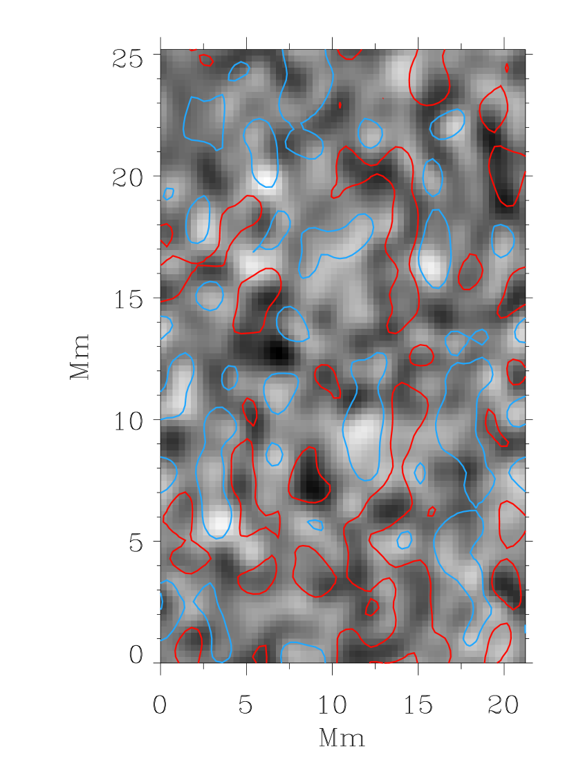
Figure 17.— Continuum intensity and Doppler velocity contours in a quiet Sun region at the solar disk center. Left: original 1″ resolution observations. The contours correspond to $\pm$250 m s^-1. Right: same observation smeared with a 2″ Gaussian, and with velocity contours at $\pm$150 m s^-1 Note the correlation between upflows (blue contours) and bright features. The correlation is not perfect, decreasing as the resolution worsens.

References

- Beckers (1977) Beckers, J. M. 1977, ApJ, 213, 900
- Beckers & Schröter (1969) Beckers, J. M., & Schröter, E. H. 1969, Sol. Phys., 10, 384
- Bellot Rubio (2004) Bellot Rubio, L. R. 2004, Rev. Mod. Astron., 17, 21
- Bellot Rubio et al. (2005) Bellot Rubio, L. R., Langhans, K., & Schlichenmaier, R. 2005, A&A, 443, L7
- Bumba (1960) Bumba, V. 1960, Izv. Crim. Astrophys. Obs., 23, 253
- Danielson (1961) Danielson, R. E. 1961, ApJ, 134, 289
- Domínguez Cerdeña et al. (2006) Domínguez Cerdeña, I., Sánchez Almeida, J., & Kneer, F. 2006, ApJ, 646, 1421
- Dravins et al. (1981) Dravins, D., Lindegren, L., & Nordlund, A. . 1981, A&A, 96, 345
- Evershed (1909) Evershed, J. 1909, MNRAS, 69, 454
- Golovko (1974) Golovko, A. A. 1974, Sol. Phys., 37, 113
- Grigorjev & Katz (1972) Grigorjev, V. M., & Katz, J. M. 1972, Sol. Phys., 22, 119
- Hurlburt et al. (2000) Hurlburt, N. E., Matthews, P. C., & Rucklidge, A. M. 2000, Sol. Phys., 192, 109
- Ichimoto (1988) Ichimoto, K. 1988, PASJ, 40, 103
- Illing et al. (1974a) Illing, R. M. E., Landman, D. A., & Mickey, D. L. 1974a, A&A, 35, 327
- Illing et al. (1974b) —. 1974b, A&A, 37, 97
- Jahn & Schmidt (1994) Jahn, K., & Schmidt, H. U. 1994, A&A, 290, 295
- Johannesson (1993) Johannesson, A. 1993, A&A, 273, 633
- Kiselman et al. (2006) Kiselman et al. 2006, in preparation, revise
- Langhans et al. (2005) Langhans, K., Scharmer, G., Kiselman, D., Löfdahl, M., & Berger, T. E. 2005, A&A, 436, 1087
- Lites (1992) Lites, B. W. 1992, in NATO ASI Ser., Vol. 375, Sunspots. Theory and Observations, ed. J. H. Thomas & N. O. Weiss (Dordrecht: Kluwer), 261
- Maltby (1964) Maltby, P. 1964, Astrophysica Norvegica, 8, 205
- Márquez et al. (2006a) Márquez, I., Bonet, J. A., Sánchez Almeida, J., & Domínguez Cerdeña, I. 2006a, in Solar Polarization 4, ed. R. Casini & B. W. Lites, ASP Conf. Ser. (San Francisco: ASP), in press
- Márquez et al. (2006b) Márquez, I., Sánchez Almeida, J., & Bonet, J. A. 2006b, ApJ, 638, 553
- Mathew et al. (2003) Mathew, S. K., Lagg, A., Solanki, S. K., Collados, M., Borrero, J. M., Berdyugina, S., Krupp, N., Woch, J., & Frutiger, C. 2003, A&A, 410, 695
- Meyer & Schmidt (1968) Meyer, F., & Schmidt, H. U. 1968, Mitteilungen der Astronomischen Gesellschaft Hamburg, 25, 194
- Nordlund (2000) Nordlund, A. 2000, Encyclopedia of Astronomy and Astrophysics, ed. P. Murdin (Bristol: IOP Publishing Ltd)
- Rimmele (1995) Rimmele, T. R. 1995, ApJ, 445, 511
- Rouppe van der Voort et al. (2004) Rouppe van der Voort, L. H. M., Löfdahl, M. G., Kiselman, D., & Scharmer, G. B. 2004, A&A, 414, 717
- Sánchez Almeida et al. (2003) Sánchez Almeida, J., Domínguez Cerdeña, I., & Kneer, F. 2003, ApJ, 597, L177
- Sánchez Almeida (1998) Sánchez Almeida, J. 1998, in ASP Conf. Ser., Vol. 155, Three-Dimensional Structure of Solar Active Regions, ed. C. E. Alissandrakis & B. Schmieder (San Francisco: ASP), 54
- Sánchez Almeida (2005) Sánchez Almeida, J. 2005, ApJ, 622, 1292
- Sánchez Almeida & Bonet (1998) Sánchez Almeida, J., & Bonet, J. A. 1998, ApJ, 505, 1010
- Sánchez Almeida et al. (1996) Sánchez Almeida, J., Landi Degl’Innocenti, E., Martínez Pillet, V., & Lites, B. W. 1996, ApJ, 466, 537
- Sánchez Almeida & Lites (1992) Sánchez Almeida, J., & Lites, B. W. 1992, ApJ, 398, 359
- Sánchez Almeida et al. (1993) Sánchez Almeida, J., Martínez Pillet, V., Trujillo Bueno, J., & Lites, B. W. 1993, in ASP Conf. Ser., Vol. 46, The Magnetic and Velocity Fields of Solar Active Regions, ed. H. Zirin, G. Ai, & H. Wang (San Francisco: ASP), 192
- Sánchez Cuberes et al. (2005) Sánchez Cuberes, M., Puschmann, K. G., & Wiehr, E. 2005, A&A, 440, 345
- Scharmer et al. (2003a) Scharmer, G. B., Bjelksjö, K., Korhonen, T. K., Lindberg, B., & Petterson, B. 2003a, Proc. SPIE, 4853, 341
- Scharmer et al. (2003b) Scharmer, G. B., Dettori, P. M., Löfdahl, M. G., & Shand, M. 2003b, Proc. SPIE, 4853, 370
- Scharmer et al. (2002) Scharmer, G. B., Gudiksen, B. V., Kiselman, D., Löfdahl, M. G., & Rouppe van der Voort, L. H. M. 2002, Nature, 420, 151
- Schlichenmaier et al. (2004) Schlichenmaier, R., Bellot Rubio, L. R., & Tritschler, A. 2004, A&A, 415, 731
- Schlichenmaier et al. (2005) —. 2005, Astronomische Nachrichten, 326, 301
- Schlichenmaier et al. (1998a) Schlichenmaier, R., Jahn, K., & Schmidt, H. U. 1998a, ApJ, 493, L121
- Schlichenmaier et al. (1998b) —. 1998b, A&A, 337, 897
- Schlichenmaier & Schmidt (1999) Schlichenmaier, R., & Schmidt, W. 1999, A&A, 349, L37
- Schlichenmaier & Schmidt (2000) Schlichenmaier, R., & Schmidt, W. 2000, A&A, 358, 1122
- Schlichenmaier & Solanki (2003) Schlichenmaier, R., & Solanki, S. K. 2003, A&A, 411, 257
- Schmidt (1991) Schmidt, H. U. 1991, Geophys. Astrophys. Fluid Dyn., 62, 249
- Schmidt et al. (1986) Schmidt, H. U., Spruit, H. C., & Weiss, N. O. 1986, A&A, 158, 351
- Schmidt & Schlichenmaier (2000) Schmidt, W., & Schlichenmaier, R. 2000, A&A, 364, 829
- Schröter (1967) Schröter, E. H. 1967, in Solar Physics, ed. J. N. Xanthakis (London: Interscience Publication), 325
- Servajean (1961) Servajean, R. 1961, Annales d’Astrophysique, 24, 1
- Sobotka et al. (1993) Sobotka, M., Bonet, J. A., & Vázquez, M. 1993, ApJ, 415, 832
- Solanki (2003) Solanki, S. K. 2003, A&A Rev., 11, 153
- Solanki & Montavon (1993) Solanki, S. K., & Montavon, C. A. P. 1993, A&A, 275, 283
- Solanki & Schmidt (1993) Solanki, S. K., & Schmidt, H. U. 1993, A&A, 267, 287
- Spruit (1987) Spruit, H. C. 1987, in The Role of Fine-Scale Magnetic Fields on the Structure of the Solar Atmosphere, ed. E.-H. Schrö ter, M. Váquez, & A. A. Wyller (Cambridge: Cambridge University Press), 199
- Spruit & Scharmer (2006) Spruit, H. C., & Scharmer, G. B. 2006, A&A, 447, 343
- Stein & Nordlund (1998) Stein, R. F., & Nordlund, Å. 1998, ApJ, 499, 914
- Stellmacher & Wiehr (1971) Stellmacher, G., & Wiehr, E. 1971, Sol. Phys., 17, 21
- Thomas & Montesinos (1993) Thomas, J. H., & Montesinos, B. 1993, ApJ, 407, 398
- Thomas & Weiss (1992) Thomas, J. H., & Weiss, N. O. 1992, in NATO ASI Ser., Vol. 375, Sunspots. Theory and Observations, ed. J. H. Thomas & N. O. Weiss (Dordrecht: Kluwer), 3
- Thomas & Weiss (2004) Thomas, J. H., & Weiss, N. O. 2004, ARA&A, 42, 517
- Tritschler et al. (2004) Tritschler, A., Schlichenmaier, R., Bellot Rubio, L. R., & the KAOS Team. 2004, A&A, 415, 717
- Weiss et al. (2004) Weiss, N. O., Thomas, J. H., Brummell, N. H., & Tobias, S. M. 2004, ApJ, 600, 1073
- Westendorp Plaza et al. (2001) Westendorp Plaza, C., del Toro Iniesta, J. C., Ruiz Cobo, B., & Martínez Pillet, V. 2001, ApJ, 547, 1148
- Wiehr (1995) Wiehr, E. 1995, A&A, 298, L17