Reducing orbital eccentricity in initial data of black hole–neutron star binaries in the puncture framework

Abstract

We develop a method to compute low-eccentricity initial data of black hole–neutron star binaries in the puncture framework extending previous work on other types of compact binaries. In addition to adjusting the orbital angular velocity of the binary, the approaching velocity of a neutron star is incorporated by modifying the helical Killing vector used to derive equations of the hydrostationary equilibrium. The approaching velocity of the black hole is then induced by requiring the vanishing of the total linear momentum of the system, differently from the case of binary black holes in the puncture framework where the linear momentum of each black hole is specified explicitly. We successfully reduce the orbital eccentricity to $\lesssim 0.001$ by modifying the parameters iteratively using simulations of $\approx 3$ orbits both for nonprecessing and precessing configurations. We find that empirical formulas for binary black holes derived in the excision framework do not reduce the orbital eccentricity to $\approx 0.001$ for black hole–neutron star binaries in the puncture framework, although they work for binary neutron stars.

I Introduction

One of the remaining and promising targets for ground-based gravitational-wave detectors is the coalescence of black hole–neutron star binaries (see Ref. Shibata and Taniguchi (2011) for reviews). Indeed, we have already been informed of possible black hole–neutron star binary coalescences in the LIGO-Virgo O3 Abbott et al. (2020a), including signals from sources whose identities are not fully clear Abbott et al. (2020b, c). If we would have detected these events with a high signal-to-noise ratio, we could infer finite-size properties of neutron stars such as the radius Vallisneri (2000); Shibata et al. (2009); Kyutoku et al. (2010, 2011); Pannarale et al. (2015) and tidal deformability Lackey et al. (2012, 2014) as well as the mass and the spin of each component. Because the finite-size properties depend crucially on the underlying equation of state for supranuclear-density matter (see Refs. Lattimer and Prakash (2016); Baym et al. (2018) for reviews), gravitational-wave observations of black hole–neutron star binaries will provide invaluable information not only to astrophysics but also to nuclear physics in a manner similar to the detections of binary neutron stars Abbott et al. (2018a, 2019a).

Reliable theoretical templates of gravitational waveforms are the prerequisite for accurate extraction of source properties Abbott et al. (2016, 2019b). Accordingly, theoretical calculations of gravitational waveforms have been playing a central role in gravitational-wave astronomy. Particularly high accuracy is required to extract finite-size properties of neutron stars, namely the tidal deformability, in a reliable manner Yagi and Yunes (2014); Favata (2014); Wade et al. (2014). Although the systematic errors associated with waveform models are smaller than the statistical errors for the first binary-neutron-star merger GW170817 Abbott et al. (2019a, 2020d); Narikawa et al. (2020) and largely uninformative GW190425 Abbott et al. (2020b), improvement of the detector sensitivity by an order of magnitude Abbott et al. (2018b) will make the systematic error discernible for GW170817-equivalent sources Kawaguchi et al. (2018); Dudi et al. (2018).

Development of templates for black hole–neutron star binaries is generally in its early stage Chakravarti et al. (2019); Huang et al. (2020) (see also Refs. Thompson et al. (2020); Matas et al. (2020) for recent progress). One reason is attributed to the small number of long-term and high-precision simulations of black hole–neutron star binaries in numerical relativity, which is the unique tool to investigate theoretically the late inspiral and merger phases and to derive gravitational waveforms. While a lot of insight on dynamical mass ejection and electromagnetic counterparts has been gained in the past years Chawla et al. (2010); Kyutoku et al. (2011); Foucart et al. (2013a); Kyutoku et al. (2013); Foucart et al. (2014); Kawaguchi et al. (2015); Kyutoku et al. (2015); Foucart et al. (2017); Kyutoku et al. (2018); Brege et al. (2018); Foucart et al. (2019a), we need to reignite numerical-relativity simulations of the inspiral and merger phases to derive accurate gravitational waveforms Foucart et al. (2013b, 2019b).

Realistic initial data of black hole–neutron star binaries are necessary to compute realistic gravitational waves in numerical relativity. In particular, the orbital eccentricity has to be low enough because the majority of astrophysical compact binaries are circularized nearly completely right before merger due to gravitational radiation reaction during its long inspiral Peters and Mathews (1963); Peters (1964). It has been pointed out that seemingly tiny eccentricity, say $e\sim 0.01$, in theoretical templates can significantly degrade the accuracy with which we can measure the tidal deformability via gravitational-wave observation Favata (2014). Eccentricity reduction has already been performed for and routinely applied to initial data of black hole–neutron star binaries in the excision framework Foucart et al. (2008), in which the physical singularity inside the horizon is removed from the computational domain. However, the eccentricity reduction for initial data of black hole–neutron star binaries in the puncture framework Shibata and Uryū (2006, 2007), in which the singularity is handled in an analytic manner, has not yet been reported.

In this paper, we present a method to reduce the orbital eccentricity in initial data of black hole–neutron star binaries in the puncture framework. Specifically, we adjust the orbital angular velocity and incorporate the approaching velocity to obtain low-eccentricity initial data, where their values are determined iteratively by analyzing orbital evolution for a few orbits derived by dynamical simulations. Differently from initial data of binary black holes in the puncture framework, in which the approaching velocity of black holes is incorporated by actively choosing the values of the linear-momentum parameter Husa et al. (2008), the translational motion of the black hole cannot be specified freely in our formulation for black hole–neutron star binaries. In this work, we first incorporate an approaching velocity of the neutron star by modifying the hydrostationary equations in the same manner as in the case of binary neutron stars Kyutoku et al. (2014a). Because the black hole is not subject to hydrodynamics, the approaching velocity of the black hole is passively induced by requiring the total linear momentum of the system to vanish. To control the approaching velocity of the binary as a whole, the velocity of the black hole is identified by the minus of the shift vector at the puncture.

The paper is organized as follows. The formulation is described in Sec. II. To demonstrate the validity of our method, we apply it to both nonprecessing and precessing configurations in Sec. III. Section IV is devoted to a summary. Greek and Latin indices denote the spacetime and space components, respectively. We adopt the geometrical unit in which $G=c=1$, where $G$ and $c$ are the gravitational constant and the speed of light, respectively.

II Numerical method

II.1 Formulation

We describe our formulation for the low-eccentricity initial data of black hole–neutron star binaries in the puncture framework. As a concise summary, the update from quasicircular initial data Kyutoku et al. (2009) resides in the modified symmetry vector, Eq. (8), which we have adopted for binary neutron stars Kyutoku et al. (2014a). Identification of the approaching velocity of the black hole, Eq. (9), has not been adopted in previous related work for compact binaries.

We compute initial data of black hole–neutron star binaries in the puncture framework Brandt and Brügmann (1997); Shibata and Uryū (2006, 2007); Shibata and Taniguchi (2008); Kyutoku et al. (2009). The singularity of gravitational fields associated with the black hole is handled in an analytic manner by decomposing geometric quantities into singular and regular parts. By adopting a mixture of extended conformal-thin sandwich formulation York (1999); Pfeiffer and York (2003) and conformal transverse-traceless decomposition York (1979), only the regular parts have to be computed numerically to satisfy Einstein constraint equations and quasiequilibrium conditions. Hydrostationary equations for the neutron-star matter are solved assuming the zero-temperature and irrotational flow Bonazzola et al. (1997); Asada (1998); Shibata (1998); Teukolsky (1998); Gourgoulhon et al. (2001), and specifically we solve the continuity equation and integrated Euler’s equation in the same manner as described in Ref. Kyutoku et al. (2014a). In this work, numerical computations are performed using a public multidomain spectral method library, LORENE LORENE website , and the details of the methods are presented in Ref. Kyutoku et al. (2009).

The puncture formulation for initial data of black hole–neutron star binaries is summarized as follows. First, conformal transformation is performed for the induced metric $\gamma_{ij}$ and the extrinsic curvature $K_{ij}$ as

$$\gamma_{ij} =\psi^{4}\hat{\gamma}_{ij},$$ (1)

$$K_{ij} =\psi^{-2}\hat{A}_{ij}+\frac{1}{3}K\psi^{4}\hat{\gamma}_{ij},$$ (2)

where $K:=\gamma^{ij}K_{ij}$. In the puncture framework, the spatial conformal flatness and maximal slicing conditions,

$$\hat{\gamma}_{ij}=f_{ij}\;,\;K=0,$$ (3)

where $f_{ij}$ is the flat metric, are imposed. We also require them to be preserved in time in the computation of initial data as usually done in the extended conformal-thin sandwich formulation (see also Refs. Wilson and Mathews (1995); Wilson et al. (1996)).

Next, we decompose the conformal factor $\psi$, a weighted lapse function $\Phi:=\alpha\psi$ with $\alpha$ being the lapse function, and the conformally weighted traceless part of the extrinsic curvature $\hat{A}_{ij}$ as

$$\psi =1+\frac{M_{\mathrm{P}}}{2r_{\mathrm{BH}}}+\phi,$$ (4)

$$\Phi =1-\frac{M_{\Phi}}{2r_{\mathrm{BH}}}+\eta,$$ (5)

$$\hat{A}_{ij} =\hat{\nabla}_{i}W_{j}+\hat{\nabla}_{j}W_{i}-\frac{2}{3}f_{ij}\hat{\nabla}^{k}W_{k}+K_{ij}^{\mathrm{P}}.$$ (6)

Here, $r_{\mathrm{BH}}$ is the coordinate distance from the puncture, $M_{\mathrm{P}}$ and $M_{\Phi}$ are constants of mass dimension, and $\hat{\nabla}_{i}$ denotes the covariant derivative associated with $f_{ij}$. The singular part of the extrinsic curvature $K_{ij}^{\mathrm{P}}$ is determined by two sets of covariantly constant vectorial parameters, namely the linear momentum $P^{\mathrm{BH}}_{i}$ and the bare spin angular momentum $S_{\mathrm{P}}^{i}$ of the black hole, as

$$K_{ij}^{\mathrm{P}} :=\frac{3}{2r_{\mathrm{BH}}^{2}}[l_{i}P^{\mathrm{BH}}_{j}+l_{j}P^{\mathrm{BH}}_{i}-(f_{ij}-l_{i}l_{j})l^{k}P^{\mathrm{BH}}_{k}]$$

$$+\frac{3}{r_{\mathrm{BH}}^{3}}[\epsilon_{kil}S_{\mathrm{P}}^{l}l^{k}l_{j}+\epsilon_{kjl}S_{\mathrm{P}}^{l}l^{k}l_{i}],$$ (7)

where $l^{i}:=x_{\mathrm{BH}}^{i}/r_{\mathrm{BH}}$ is the unit radial vector, $l_{i}=f_{ij}l^{j}$, and $\epsilon_{ijk}$ is the Levi-Civita tensor associated with $f_{ij}$ Bowen and York (1980); Brandt and Brügmann (1997).

Finally, the regular parts of the geometric quantities $\phi$, $\eta$, $W_{i}$, and the shift vector $\beta^{i}$ are obtained by solving elliptic equations derived from a subset of the Einstein equation [see, e.g., Eqs. (16)–(19) of Ref. Kyutoku et al. (2009) for the explicit form]. In the puncture framework, we have no inner boundary at the horizon, and the outer boundary condition is derived from the asymptotic flatness condition.

One of the keys to obtain low-eccentricity initial data is incorporation of the approaching velocity to the helical symmetry, which governs quasicircular initial data of binaries. Following Ref. Kyutoku et al. (2014a), we adopt a symmetry vector equipped with the approaching velocity $v_{\mathrm{app,NS}}^{i}$ of the form

$$\xi^{\mu}=(\partial_{t})^{\mu}+\Omega(\partial_{\varphi})^{\mu}+v_{\mathrm{app,NS}}^{i}(\partial_{i})^{\mu}$$ (8)

around the neutron star. In our computation, the rotational axis is taken to be the $z$ axis, and both the black hole and the neutron star are chosen to be located on the $xz$ plane. That is, we have $x_{\mathrm{NS}}^{i}=(x_{\mathrm{NS}},0,z_{\mathrm{NS}})$ and $x_{\mathrm{BH}}^{i}=(x_{\mathrm{BH}},0,z_{\mathrm{BH}})$. We always choose $z_{\mathrm{NS}}=0$ without loss of generality because this choice removes the need for moving fluid variables as a whole during the iteration. For nonprecessing configurations, we also set $z_{\mathrm{BH}}=0$ and thus both members of the binary are located on the $x$ axis. Our symmetry vector with a translational approaching motion is slightly different from the uniform contraction usually adopted in other eccentricity reduction methods Pfeiffer et al. (2007); Foucart et al. (2008); Buonanno et al. (2011), and no significant difference has been found for binary neutron stars Kyutoku et al. (2014a). We note that this modified symmetry vector is not fully compatible with the spacetime symmetry as discussed in Ref. Kyutoku et al. (2014b).

II.2 Choice of free parameters

Table 1: Free parameters and requirements for determining them in our formulation for initial data of black hole–neutron star binaries in the puncture framework. Because $\Omega$ is determined in a different manner for quasicircular and low-eccentricity initial data, we show two conditions separately by “QC” and “low-$e$,” respectively. The approaching velocity of the neutron star, $v_{\mathrm{app,NS}}^{i}$, is fixed to be zero for quasicircular initial data.

Symbol and meaning	Requirement
Parameters of the black hole
$M_{\mathrm{P}}$: bare mass parameter in $\psi$	The mass of the black hole takes a desired value
$S_{\mathrm{P}}^{i}$: bare spin parameter in $K^{\mathrm{P}}_{ij}$	The spin vector of the black hole takes a desired value
$P^{\mathrm{BH}}_{i}$: linear-momentum parameter in $K^{\mathrm{P}}_{ij}$	The total linear momentum of the system vanishes
$M_{\Phi}$: mass parameter in $\Phi$	The Arnowitt-Deser-Misner and Komar masses agree
Parameters of the neutron star
$-hu_{\mu}\xi^{\mu}$: first integral of Euler’s equation	The mass of the neutron star takes a desired value
$v_{\mathrm{app,NS}}^{i}$: approaching velocity	The approaching velocity of the binary takes a desired value
Parameters of the binary
$d^{x}$: separation along the $x$ axis	This is fixed to specify a model
$d^{z}$: separation along the $z$ axis	The force-balance condition along the $z$ direction is satisfied
$\Omega$: orbital angular velocity	QC: The force-balance condition along the $x$ direction is satisfied
	low-$e$: This is fixed to a desired value
Location of the rotational axis	The azimuthal component of the shift vector at the puncture is equal to $-\Omega$

Free parameters in the formulation must be determined by physical requirements. In this subsection, we describe our method for determining them. A concise summary is presented in Table 1. Iterative procedures are described in Sec. III B of Ref. Kyutoku et al. (2009) except that we have included steps to adjust the approaching velocity and the value of $z_{\mathrm{BH}}$. The level of the convergence for our iterative solution is not affected significantly by the eccentricity reduction procedure.

The bare mass, $M_{\mathrm{P}}$, and the bare spin parameter, $S_{\mathrm{P}}^{i}$, are determined to obtain desired values of the mass and spin of the black hole. The mass and spin magnitude of the black hole are computed in the isolated-horizon framework (see Ref. Gourgoulhon and Jaramillo (2006) for reviews) with an approximate rotational Killing vector obtained by minimizing its shear on the horizon Cook and Whiting (2007). In our computation, we restrict the spin parameter to have only $x$ and $z$ components and define the inclination angle $\iota$ as the angle between the coordinate components of the orbital angular momentum and the spin angular momentum in a gauge-dependent manner Kawaguchi et al. (2015). The linear momentum of the black hole, $P^{\mathrm{BH}}_{i}$, is determined by requiring the total linear momentum of the system vanishes. This means that we cannot choose values of $P^{\mathrm{BH}}_{i}$ to control the approaching velocity of the black hole. This is the chief difference from the eccentricity reduction of binary black holes in the puncture framework Husa et al. (2008); Pürrer et al. (2012); Ramos-Buades et al. (2019) and is the reason that we need to develop a method suitable for black hole–neutron star binaries. A constant value of the first integral of the Euler equation, $-hu_{\mu}\xi^{\mu}$ with $h$ and $u^{\mu}$ being the specific enthalpy and the $4$-velocity of the fluid, respectively, is determined by requiring the baryon rest mass of the neutron star to take a desired value.

The mass parameter in the weighted lapse function, $M_{\Phi}$, is determined by the condition that the Arnowitt-Deser-Misner and Komar masses agree, which holds for stationary and asymptotically flat spacetimes Beig (1978); Ashtekar and Magnon-Ashtekar (1979). This condition also holds for quasicircular initial data computed in our formulation Friedman et al. (2002); Shibata et al. (2004), and thus requiring this condition is fully justified (see also Refs. Gourgoulhon et al. (2002); Grandclément et al. (2002); Caudill et al. (2006) for early work on binary black holes). However, this does not hold rigorously for low-eccentricity initial data with an approaching velocity. Despite this caveat, we still determine the value of $M_{\Phi}$ by the equality of the two masses even if the approaching velocity is turned on. We expect that this condition is not very problematic because we observe for initial data of binary neutron stars Kyutoku et al. (2014a) that the differences between the Arnowitt-Deser-Misner and Komar masses are of the same order for both quasicircular and low-eccentricity cases. This situation is also reported in black hole–neutron star initial data computed in the excision framework Foucart et al. (2008). When more accurate numerical computations become necessary, the condition for determining $M_{\Phi}$ should be elaborated. The Arnowitt-Deser-Misner and Komar masses are computed both by surface and volume integrals, and these two variants agree within the error of $O(${10}^{-6}$)$.

As we will discuss in the next section, we would like to control the orbital angular velocity $\Omega$ and approaching velocity of the binary $v_{\mathrm{app}}$ to obtain low-eccentricity initial data. On one hand, the orbital angular velocity, $\Omega$, appears explicitly in our symmetry vector, Eq. (8). On the other hand, the approaching velocity of the binary is controlled implicitly via that of the neutron star, $v_{\mathrm{app,NS}}^{i}$, in our formulation. The approaching velocity vector of the black hole, $v_{\mathrm{app,BH}}^{i}$, in the initial data is identified as the minus of the $x$ and $z$ components (see below for the $y$ component) of the shift vector at the puncture as

$$v_{\mathrm{app,BH}}^{i}=\left.(-\beta^{x},0,-\beta^{z})\right|_{\mathrm{BH}}.$$ (9)

Then, we adjust the value of $|v_{\mathrm{app,NS}}^{i}|$, where the usual Euclidean norm is assumed, so that $|v_{\mathrm{app,NS}}^{i}|+|v_{\mathrm{app,BH}}^{i}|$ agrees with the desired value of $|v_{\mathrm{app}}|$. Although we could have adjusted the value of $|v_{\mathrm{app,NS}}^{i}-v_{\mathrm{app,BH}}^{i}|$ instead, this is not necessarily preferable in a curved spacetime. Because we always require the vanishing of the total linear momentum of the system, the approaching velocity of the neutron star automatically induces that of the black hole.

When we compute quasicircular initial data for a given separation along the $x$ axis, $d^{x}$, the value of $\Omega$ is determined by requiring the force balance at the neutron-star center (see Sec. IV D 2 of Ref. Gourgoulhon et al. (2001)),

$$\left.\frac{\partial h}{\partial x}\right|_{\mathrm{NS}}=0.$$ (10)

Specifically, we insert constancy of the first integral of the Euler equation to Eq. (10). Because the first integral of the Euler equation includes $\Omega$ through the shift vector, the force balance condition, Eq. (10), can be rewritten as an equation to determine the orbital angular velocity. The approaching velocity is set to be zero by choosing $v_{\mathrm{app,NS}}^{i}=0$. This results in $v_{\mathrm{app,BH}}^{i}=0$ within the numerical error.

When we compute low-eccentricity initial data for a given value of $d^{x}$, we prescribe desired values of $\Omega$ and $v_{\mathrm{app}}$ according to the estimates from dynamical simulations (see Sec. II.3). The value of $\Omega$ in Eq. (8) is fixed to this prescribed value for each computation of initial data. For the approaching velocity vector of the neutron star, $v_{\mathrm{app,NS}}^{i}$, in Eq. (8), we need to determine the magnitude and the direction. The magnitude is determined so that $|v_{\mathrm{app,NS}}^{i}|+|v_{\mathrm{app,BH}}^{i}|$ takes the prescribed value, $|v_{\mathrm{app}}|$. The direction is set to point toward the black hole. For nonprecessing binaries, $v_{\mathrm{app,NS}}^{i}$ has only the $x$ component and $v_{\mathrm{app,BH}}^{i}$ points exactly opposite to $v_{\mathrm{app,NS}}^{i}$. For precessing binaries, we find that the induced approaching velocity of the black hole, $v_{\mathrm{app,BH}}^{i}$, does not point exactly toward the neutron star in our coordinates, but the deviation is smaller than $0.1\mathrm{°}$ for the case studied here. Because the direction is inherently gauge dependent, we regard this deviation as acceptable.

We have to determine the location of the rotational axis, or the positions of the black hole and neutron star relative to the rotational axis, in our computations. In the excision framework, this location is fixed by the condition that the total linear momentum of the system vanishes Taniguchi et al. (2006, 2007, 2008); Foucart et al. (2008). However, this condition has already been used to determine $P^{\mathrm{BH}}_{i}$ in the puncture framework. In this work, following Ref. Shibata and Taniguchi (2008), we determine the location of the rotational axis by requiring that the azimuthal component of the shift vector at the puncture is equal to the minus of the angular velocity,

$$\left.\beta^{\varphi}\right|_{\mathrm{BH}}=-\Omega.$$ (11)

This states that the puncture moves along the symmetry vector, Eq. (8), and is consistent with our definition of $v_{\mathrm{app,BH}}^{i}$, where the unused $y$ component of the shift vector is interpreted as the orbital velocity.

We also have to determine the separation between the black hole and the neutron star along the rotational axis, $d^{z}$, when we compute precessing configurations. It is determined by requiring the force-balance condition like Eq. (10) but along the $z$ direction Foucart et al. (2011); Kawaguchi et al. (2015),

$$\left.\frac{\partial h}{\partial z}\right|_{\mathrm{NS}}=0.$$ (12)

The position of the neutron star is fixed to $z_{\mathrm{NS}}=0$ throughout.

II.3 Iterative correction

We seek the optimal choice of $\Omega$ and $v_{\mathrm{app}}$ for a given value of the separation along the $x$ axis, $d^{x}$, via iterative corrections estimated from the orbital evolution derived by dynamical simulations. This strategy is originally developed for binary-black-hole initial data Pfeiffer et al. (2007) and later applied successfully to black hole–neutron star binaries in the excision framework Foucart et al. (2008) and to binary neutron stars Kyutoku et al. (2014a); Moldenhauer et al. (2014); Haas et al. (2016). Our dynamical simulations are performed with an adaptive-mesh-refinement code, SACRA Yamamoto et al. (2008), and the formulation adopted in the current version is explained in Ref. Kyutoku et al. (2014a). We do not use the MPI-parallelized version of SACRA Kiuchi et al. (2017) because the eccentricity reduction does not require orbital evolution with a very high precision.

The position and velocity of the neutron star are identified with the integration over the fluid as

$$x_{\mathrm{NS}}^{i} =\frac{\int\rho_{*}x^{i}d^{3}x}{\int\rho_{*}d^{3}x},$$ (13)

$$\dot{x}_{\mathrm{NS}}^{i} =\frac{\int\rho_{*}\dot{x}^{i}d^{3}x}{\int\rho_{*}d^{3}x},$$ (14)

where $\rho_{*}:=\rho\alpha u^{t}\sqrt{\gamma}$ and $\dot{x}^{i}:=u^{i}/u^{t}$, with $\rho$ being the rest-mass density. The velocity of the black hole is identified as the minus of the shift vector at the puncture in a manner similar to Eq. (9) as

$$\dot{x}_{\mathrm{BH}}^{i}=\left.-\beta^{i}\right|_{\mathrm{BH}},$$ (15)

and the position is obtained by integrating this in time Campanelli et al. (2006); Brügmann et al. (2008). In SACRA, the shift vector at the puncture is determined by trilinear interpolation from surrounding eight grid points, and this limits the accuracy with which we can determine the orbital evolution for given data of gravitational fields. The orbital angular velocity of the binary is computed from the Euclidean outer product of $x^{i}:=x_{\mathrm{NS}}^{i}-x_{\mathrm{BH}}^{i}$ and $\dot{x}^{i}:=\dot{x}_{\mathrm{NS}}^{i}-\dot{x}_{\mathrm{BH}}^{i}$ as Buonanno et al. (2011); Boyle (2013)

$$\mathbf{\Omega}=\frac{\mathbf{x}\times\dot{\mathbf{x}}}{|\mathbf{x}|^{2}}.$$ (16)

We estimate appropriate values of the correction to $\Omega$ and $v_{\mathrm{app}}$ by fitting the time evolution of orbital angular velocity, $\dot{\Omega}(t)$, by a function Pfeiffer et al. (2007); Boyle et al. (2007); Buonanno et al. (2011)

$$\dot{\Omega}(t)=A_{0}+A_{1}t+B\cos(\omega t+\phi_{0}),$$ (17)

where $\{A_{0},A_{1},B,\omega,\phi_{0}\}$ are parameters determined by the fitting. We average numerical data over $\sim 100$ time steps in deriving $\dot{\Omega}(t)$ to remove high-frequency noise Kyutoku et al. (2014a). The fitting is performed using $\dot{\Omega}(t)$ during $0.5P_{0}<t<3P_{0}$, where $P_{0}$ is the initial orbital period of the binary. Aiming at removing the modulation term, $B\cos(\omega t+\phi_{0})$, we modify $\Omega$ and $v_{\mathrm{app}}$ in the initial-data computation by

$$\delta\Omega =-\frac{B\omega\sin\phi_{0}}{4\Omega^{2}},$$ (18)

$$\delta v_{\mathrm{app}} =\frac{Bd\cos\phi_{0}}{2\Omega},$$ (19)

according to Newtonian expressions Pfeiffer et al. (2007); Buonanno et al. (2011); Kyutoku et al. (2014a). Here, $d=\sqrt{(d^{x})^{2}+(d^{z})^{2}}=|x^{i}(t=0)|$ is the initial orbital separation. We also estimate the orbital eccentricity by

$$e\approx\frac{|B|}{2\omega\Omega}$$ (20)

in this fitting procedure. Exceptionally when $e\lesssim 0.001$, we find that the beginning of the fitting interval has to be delayed until $t=0.75P_{0}$ to obtain meaningful estimates of the residual eccentricity.

III Demonstration

Table 2: Key quantities of the models of black hole–neutron star binaries constructed in this work. Names of models represent the spin configuration and the stage of eccentricity reduction. Specifically, QC and IterX stand for quasicircular and the Xth iteration, respectively. The total mass of the binary at infinite separation, $m_{0}$, is $5.4M_{\odot}$ for all the models. The normalized orbital angular velocity $m_{0}\Omega$ and approaching velocity $v_{\mathrm{app}}$ of the binary characterize the initial data. The Arnowitt-Deser-Misner mass is denoted by $M_{0}$, where we show it as the gravitational binding energy, $|M_{0}-m_{0}|$. The magnitude of the orbital angular momentum of the system is given by $L_{0}$, which does not include the spin angular momentum of the black hole. The eccentricity $e$ is estimated by fitting the time derivative of the orbital angular velocity obtained in dynamical simulations. The initial orbital period, gravitational-wave frequency, and wavelength are $\approx$6.7\text{\,}\mathrm{ms}$,\approx$300\text{\,}\mathrm{Hz}$$, and $\approx$1000\text{\,}\mathrm{km}$$, respectively.

Model	$m_{0}\Omega$	$v_{\mathrm{app}}$	$|M_{0}-m_{0}|(M_{\odot})$	$L_{0}(M_{\odot}^{2})$	$e$
Zero Spin: $\chi=0,d=$86.1\text{\,}\mathrm{km}$$
ZS-QC	$0.0250001$	$0$	$0.0399$	$21.29$	$0.04$
ZS-Iter1	$0.0252757$	$-0.00723672$	$0.0388$	$21.54$	$0.02$
ZS-Iter2	$0.0254085$	$-0.00233390$	$0.0382$	$21.66$	$0.006$
ZS-Iter3	$0.0253783$	$-0.00138723$	$0.0384$	$21.63$	$0.003$
ZS-Iter4	$0.0253797$	$-0.00207750$	$0.0384$	$21.63$	$0.003$
ZS-Iter5	$0.0253657$	$-0.00173550$	$0.0384$	$21.62$	$0.0005$
Aligned Spin: $\chi=0.75,\iota=$$,d=$85.5\text{\,}\mathrm{km}$$
AS-QC	$0.0249999$	$0$	$0.0416$	$20.36$	$0.04$
AS-Iter1	$0.0253334$	$-0.00713689$	$0.0403$	$20.65$	$0.02$
AS-Iter2	$0.0254891$	$-0.00264875$	$0.0396$	$20.79$	$0.007$
AS-Iter3	$0.0254545$	$-0.00097836$	$0.0398$	$20.75$	$0.003$
AS-Iter4	$0.0254355$	$-0.00160145$	$0.0399$	$20.74$	$0.002$
AS-Iter5	$0.0254308$	$-0.00194680$	$0.0399$	$20.73$	$0.002$
AS-Iter6	$0.0254454$	$-0.00164779$	$0.0398$	$20.75$	$0.002$
AS-Iter7	$0.0254302$	$-0.00177446$	$0.0399$	$20.73$	$0.001$
AS-Iter8	$0.0254431$	$-0.00174272$	$0.0398$	$20.74$	$0.002$
AS-Iter9	$0.0254245$	$-0.00165976$	$0.0399$	$20.73$	$0.0008$
Inclined Spin: $\chi=0.75$, $\iota\approx$$,d^{x}=$86.0\text{\,}\mathrm{km}$,d^{z}\approx$3.5\text{\,}\mathrm{km}$$
IS-QC	$0.0250000$	$0$	$0.0399$	$21.27$	$0.04$
IS-Iter1	$0.0252851$	$-0.00742954$	$0.0387$	$21.53$	$0.03$
IS-Iter2	$0.0254223$	$-0.00246477$	$0.0382$	$21.65$	$0.006$
IS-Iter3	$0.0253949$	$-0.00139129$	$0.0383$	$21.62$	$0.003$
IS-Iter4	$0.0253965$	$-0.00217036$	$0.0383$	$21.63$	$0.003$
IS-Iter5	$0.0253833$	$-0.00166181$	$0.0383$	$21.61$	$0.0008$

We present results of our eccentricity reduction for a few models of black hole–neutron star binaries. Key quantities of the initial data constructed in this work are summarized in Table 2. The neutron stars are modeled by a piecewise polytropic approximation Read et al. (2009) of the APR4 equation of state Akmal et al. (1998) with the gravitational mass in isolation of $M_{\mathrm{NS}}=1.35M_{\odot}$. The APR4 equation of state is consistent with GW170817 De et al. (2018); Abbott et al. (2018a, 2019a, 2020d); Narikawa et al. (2020) and gives the dimensionless tidal deformability of $323$ for this $1.35M_{\odot}$ neutron star. The gravitational mass in isolation of the black hole is fixed to be $M_{\mathrm{BH}}=4.05M_{\odot}$, giving the mass ratio $Q:=M_{\mathrm{BH}}/M_{\mathrm{NS}}=3$, which has been studied vigorously in the literature. Accordingly, the total mass at infinite separation $m_{0}:=M_{\mathrm{BH}}+M_{\mathrm{NS}}$ is $5.4M_{\odot}$. We have checked that our eccentricity reduction method works similarly for other equations of state and/or binary parameters at least for the range considered in our previous work Kyutoku et al. (2015) (see Ref. Kyutoku et al. (2014a) for binary neutron stars). We plan to present results of systematic long-term simulations of low-eccentricity black hole–neutron star binary coalescences elsewhere.

All the simulations are performed with computational domains consisting of five coarser boxes fixed around an approximate center of mass and four pairs of finer boxes comoving with each binary component. The edge length of the largest computational domain is $\approx$2500\text{\,}\mathrm{km}$$ and the grid resolution at the finest domain is $\approx$240\text{\,}\mathrm{m}$$. With this resolution, the coordinate radius of the neutron star is covered by $\approx 35$ points, and that of the apparent horizon is covered by $\approx 25$ and $18$ points for $\chi=0$ and $0.75$, respectively. The grid resolution is intentionally kept moderate for demonstrating that the eccentricity reduction can be performed with a reasonable computational cost. We checked for selected models, both before and after the eccentricity reduction, that the eccentricity does not depend on the grid resolution of the dynamical simulations.

III.1 Nonprecessing case

First, we apply the eccentricity reduction described in Sec. II to two nonprecessing binaries. One is the ZS (zero spin) model, for which the black hole is nonspinning. The other is the AS (aligned spin) model, for which the black hole is spinning in a prograde sense with respect to the orbital angular momentum with its magnitude being $\chi=0.75$. (See the next subsection for IS.) The orbital modulation is induced only by the residual eccentricity and possible gauge artifacts (see, e.g., Refs. Pürrer et al. (2012); Kyutoku et al. (2014a)) for these models. Thus, the eccentricity reduction should be straightforward.

III.1.1 Time evolution

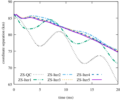
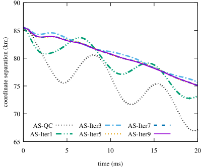
Figure 1: Time evolution of the orbital separation for the ZS (left) and AS (right) families during initial $\approx 3$ orbital cycles. The eccentricity-induced modulation has a longer period than the orbital period due to the periastron advance. Differently from Ref. Kyutoku et al. (2014a), we do not need to perform Bezier smoothing to eliminate high-frequency noises because the location of the neutron star is defined not by the maximum density on discrete grid points but by the integral, Eq. (13). Dips seen during the first $2$–$3\text{\,}\mathrm{ms}$ reflect initial gauge transition.

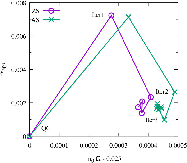
Figure 2: Orbital angular velocity and approaching velocity of initial data for the ZS (circle) and AS (cross) families. The former is plotted as the difference from $0.025$ of a value normalized by the total mass of the binary, $m_{0}$, and the latter is given by its negative. The origin represents the QC data, and successive points correspond to the data of subsequent iteration stages. We do not attach labels to data beyond Iter3 to avoid overcrowding.

Figure 1 shows the time evolution of the orbital separation for selected models in the sequence of eccentricity reduction. The orbital eccentricity is reduced from $~{}0.04$ to $<0.001$ (see Table 2) by several iterative corrections. To achieve this eccentricity with current models, for which $m_{0}\Omega\approx 0.025$, we need to modify the orbital angular velocity by $\approx 1.5\%$–1.7% and to add the approaching velocity of $\approx 0.17\%$ of the speed of light. While the required approaching velocity is similar to the value found for binary neutron stars considered in Ref. Kyutoku et al. (2014a), the fractional amount of the required correction to the orbital angular velocity, $\delta\Omega/\Omega$, is larger by a factor of $\approx 4$. This is consistent with the degree of the residual eccentricity, which is also higher by a factor of $\approx 4$ than that of binary neutron stars, $e\approx 0.01$, for quasicircular initial data considered in Ref. Kyutoku et al. (2014a), because Eqs. (18) and (20) indicate that these quantities are approximately proportional to each other. The approaching velocity may play a subdominant role for determining the residual eccentricity.

The number of required iterations is typically larger than that for binary neutron stars with our method Kyutoku et al. (2014a). Changes of the relevant parameters during the eccentricity reduction are presented graphically in Fig. 2, which should be compared with Fig. 1 of Ref. Kyutoku et al. (2014a). This difference means that the eccentricity reduction is cumbersome for black hole–neutron star binaries, which are highly asymmetric and involve singularities associated with the puncture. The necessity of many iterations is partly ascribed to larger eccentricities in quasicircular initial data of black hole–neutron star binaries in the puncture framework described above. Another reason may be that our current correction formulas, Eqs. (18) and (19), are not efficient at $e\lesssim 0.2\%$–0.3%. The situation is visualized as wandering of points beyond Iter3 in Fig. 2. This low efficiency may be ascribed to the fact that initial transition of the gauge condition in the simulations (see Fig. 1) limits the accuracy with which we can extrapolate results of the fitting to $t=0$ Pürrer et al. (2012). Our results also suggest that the presence of a black hole spin increases the computational cost for the eccentricity reduction, and indeed our experience supports this observation.

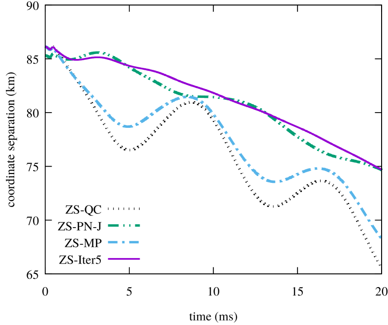
Figure 3: Same as Fig. 1 but for different initial data of the ZS model. The curve labeled by ZS-PN-J shows the result for quasicircular initial data for which the location of the rotational axis is determined by the PN-J condition (see the body text). That labeled by ZS-MP shows the result for low-eccentricity initial data whose parameters are given by the fitting formulas due to Ref. Mroué and Pfeiffer (2012).

We recall that the orbital eccentricity of quasicircular initial data, i.e., those without the approaching velocity, can be reduced by a factor of 2–3 compared to the QC data adopted in this study simply by changing the condition to determine the location of the rotational axis Shibata et al. (2009); Kyutoku et al. (2009). We compare orbital evolution derived with various quasicircular initial data as well as low-eccentricity ones for ZS models in Fig. 3. Here, the PN-J model refers to quasicircular initial data in which the location of the rotational axis is determined by requiring that the total angular momentum of the system agrees with post-Newtonian predictions Kyutoku et al. (2009), while the QC model is derived using Eq. (11). No iterative eccentricity reduction is applied to either initial data. This figure shows that the PN-J data are superior to the QC data but cannot be a substitute for low-eccentricity initial data, ZS-Iter5. At the same time, this figure suggests that the eccentricity reduction described in this work may further be improved by modifying the method to determine the location of the rotational axis. In addition, the number of required iterations may be reduced by changing the method appropriately. We leave this topic as a future task.

We also find that phenomenological formulas for $\Omega$ and $v_{\mathrm{app}}$ derived by simulations of binary-black-hole mergers in the excision framework Mroué and Pfeiffer (2012) do not reduce the orbital eccentricity of black hole–neutron star binaries in the puncture framework to $\lesssim 0.001$, although they work successfully for binary neutron stars Hotokezaka et al. (2015, 2016); Kiuchi et al. (2017, 2020). The orbital evolution is shown in Fig. 3 as ZS-MP. The eccentricity of this model is only smaller by a factor of $\lesssim 2$ than that of ZS-QC. This inefficiency may be ascribed to different approaches for handling black holes, i.e., the puncture or excision. Actually, it has been shown in the study of quasiequilibrium sequences that the puncture initial data are characterized by insufficient orbital angular momenta compared to the excision initial data and post-Newtonian predictions Kyutoku et al. (2009). Thus, it is naturally expected that the parameters to achieve low eccentricity depend significantly on the framework to handle the black hole.

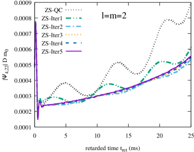
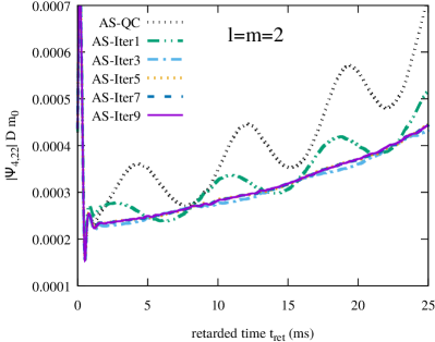
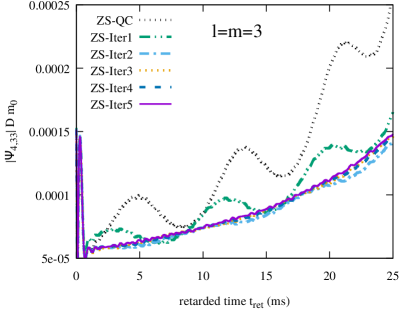
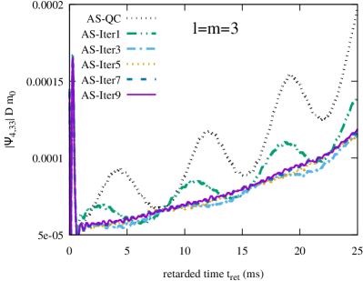
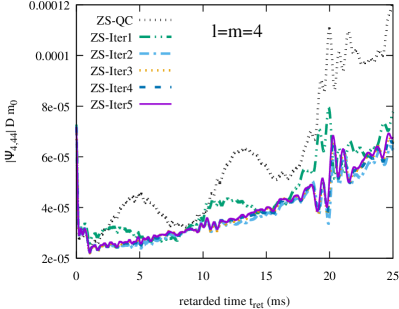
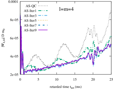
Figure 4: Time evolution of the mode amplitude of $\Psi_{4}$ normalized by $Dm_{0}$ for the ZS (left) and AS (right) families. The top, middle, and bottom rows show the $l=m=2,3,$ and $4$ modes, respectively. The initial $\approx$1\text{\,}\mathrm{ms}$$ suffers from junk radiation in the initial data. Wiggles observed in our previous work Kyutoku et al. (2014a) are not significant for the $l=m=2$ mode because the extraction radii are larger by a factor of $\approx 4$ here. Still, they are discernible in higher harmonics.

To demonstrate that the successful reduction of the eccentricity is not a gauge artifact, we also show the time evolution of the mode amplitude of a Weyl scalar $\Psi_{4}$ as a gauge-invariant quantity in Fig. 4. The time coordinate is taken to be a retarded time defined by

$$t_{\mathrm{ret}} :=t-D-2m_{0}\ln(D/m_{0}),$$ (21)

$$D :=r_{\mathrm{ext}}\left(1+\frac{m_{0}}{2r_{\mathrm{ext}}}\right)^{2},$$ (22)

where $r_{\mathrm{ext}}=800M_{\odot}=$1181\text{\,}\mathrm{km}$$ is the extraction radius. The suppression of the modulation in $\Psi_{4}$ confirms that the reduced orbital modulation shown in Fig. 1 is a physical outcome caused by the reduced eccentricity. This figure also shows that the modulation is eliminated irrespective of the harmonic modes. This is particularly important for asymmetric systems like black hole–neutron star binaries, for which higher multipole modes are prominent in the actual gravitational-wave signals Abbott et al. (2020c, e).

III.1.2 Properties of initial data

We briefly comment on notable features of initial data. The eccentricity reduction decreases the absolute value of the binding energy and increases the orbital angular momentum of the binary (e.g., compare ZC-QC and ZC-Iter5). Although it is not as good as in the case of binary neutron stars Kyutoku et al. (2014a), the agreement of the angular momentum between our numerical initial data and post-Newtonian approximations is improved by a factor of $\approx 3$ by the eccentricity reduction. Quantitatively, for $\chi=0$ associated with the ZS model, fourth post-Newtonian approximations give $|M_{0}-m_{0}|=0.0394M_{\odot}$ and $L_{0}=21.59M_{\odot}^{2}$ for $m_{0}\Omega=0.025$ Blanchet (2014), where the tidal effect does not significantly affect these values Vines and Flanagan (2013). For an updated value of $m_{0}\Omega=0.0253657$ corresponding to ZS-Iter5, post-Newtonian approximations give $|M_{0}-m_{0}|=0.0397M_{\odot}$ and $L_{0}=21.52M_{\odot}^{2}$.

The increase of the angular momentum for low-eccentricity initial data is consistent with our previous finding that the eccentricity in quasicircular initial data can be reduced by enhancing the angular momentum via the condition to determine the location of the rotational axis Shibata et al. (2009); Kyutoku et al. (2009). However, the binding energy for low-eccentricity initial data tends to deviate more from the post-Newtonian predictions than that for quasicircular initial data. The insufficient binding of the low-eccentricity initial data is consistent with our previous work Kyutoku et al. (2009) and may reflect an inherent limitation of initial data for black hole–neutron star binaries in the puncture framework.

We find that junk radiation may account for a significant fraction of the differences in the binding energy and the orbital angular momentum. Specifically, the junk radiation is found to carry away the energy $\Delta E\approx 4$–$$5\text{\times}{10}^{-4}$M_{\odot}$ and the angular momentum $\Delta L\approx 5$–$$6\text{\times}{10}^{-2}$M_{\odot}^{2}$ irrespective of the residual eccentricity for the ZS family. They correspond to $\approx 30\%$–40% for the binding energy and $\approx 50\%$–60% for the orbital angular momentum of the differences between ZS-Iter5 and the post-Newtonian predictions. For ZC-QC, taking into account the junk radiation only increases the differences.

The agreement of the angular momentum is improved only moderately for spinning black hole–neutron star binaries. For $\chi=0.75$ associated with the AS model and $m_{0}\Omega=0.025$, the post-Newtonian prediction gives $|M_{0}-m_{0}|=0.0413M_{\odot}$ and $L_{0}=20.63M_{\odot}^{2}$, where the spin effect is included up to 3.5th order Bohé et al. (2013); Blanchet (2014). These values change to $|M_{0}-m_{0}|=0.0417M_{\odot}$ and $L_{0}=20.54M_{\odot}^{2}$ for $m_{0}\Omega=0.0254245$ corresponding to AS-Iter9. In addition, the binding energy of quasicircular initial data appears closer to the post-Newtonian prediction than that of low-eccentricity initial data is. Still, our results indicate that the key to reduce the eccentricity is to enhance the orbital angular momentum and the binding energy from quasicircular initial data derived with the helical symmetry.

Again, junk radiation may account for a significant fraction of the difference between AS-Iter9 and the post-Newtonian predictions. In particular, the energy carried away by the junk radiation is $\Delta E\approx$2\text{\times}{10}^{-3}$M_{\odot}$ and agrees approximately with the difference in the binding energy. On another front, the angular momentum carried away by the junk radiation is $\Delta L\approx 5$–$$6\text{\times}{10}^{-2}$M_{\odot}^{2}$, approximately coinciding with the value for the ZS family. This account for $\approx 30\%$ of the difference.

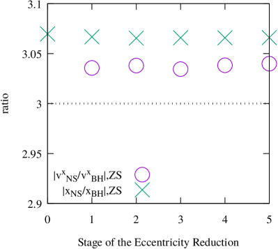
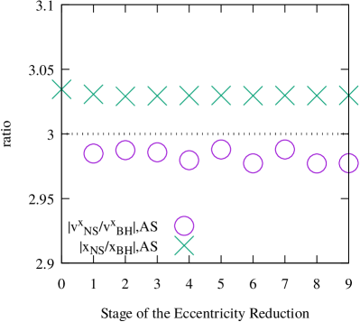
Figure 5: Ratio of the approaching velocity (circle) and position (cross) between the neutron star and the black hole for the ZS (left) and AS (right) families. The horizontal axis denote the stage of iterative corrections with $0$ being the QC data. The dotted lines denote $Q=3$.

Finally, as we do not have a direct control of $v_{\mathrm{app,BH}}^{i}$, it is worthwhile to check whether the approaching velocity of the binary in the initial data is reasonably distributed to the black hole and the neutron star with the ratio around an expected value of $Q=3$. Figure 5 shows the ratio of the $x$ components of the velocity as well as the $x$ coordinates for ZS and AS families. This figure indicates that the reasonable distribution is automatically achieved. Because both the velocity and the position are gauge-dependent quantities, we believe that the deviation of 1%–2% from $Q=3$ found here is acceptable.

III.2 Precessing case

Next, we perform eccentricity reduction on precessing binaries, for which the black hole spin angular momentum is inclined with respect to the orbital angular momentum of the binary. The spin-orbit, spin-spin, and quadrupole-monopole couplings induce orbital precessions for inclined spins Barker and O’Connell (1975); Apostolatos et al. (1994); Racine (2008), and precession-induced modulation appears in the orbital evolution and gravitational waves Buonanno et al. (2011). This feature could make the eccentricity reduction more complicated than in the cases of nonprecessing binaries.

We specifically consider the IS (inclined spin) model, for which the black hole spin of $\chi=0.75$ is inclined toward the neutron star by $\approx$$$ from the initial orbital angular momentum in the initial data. This model is expected to exhibit precession of the orbital plane with the period $\approx$130\text{\,}\mathrm{ms}$$, which decreases during the orbital evolution. Following Ref. Kawaguchi et al. (2015), the $z$ axis of the dynamical simulation is taken to be the direction of the total angular momentum, which is approximately fixed throughout the evolution.

III.2.1 Time evolution

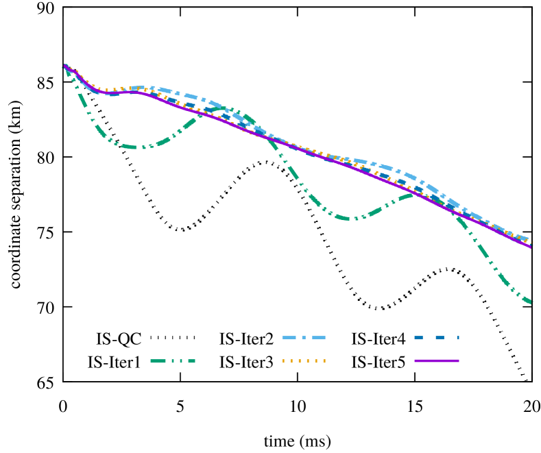
Figure 6: Same as Fig. 1 but for the IS family. The orbital plane is expected to exhibit $\sim 20\%$ of the precession cycle on the time scale of this plot.

Figure 6 shows the time evolution of the orbital separation for the IS family. This indicates that the performance of our eccentricity reduction is similar to that for the ZS family. The evolution of the orbital separation itself is also similar to that of the ZS model because the black hole spin is approximately confined in the orbital plane so that the inspiral is not decelerated or accelerated by the spin-orbit interaction Kidder (1995). Because we aim only at reducing the orbital eccentricity to a moderately low value of $\lesssim 0.001$, the precession-induced modulation does not appear even in our low-eccentricity evolution. We have checked that we did not incorrectly subtract the precession-induced modulation during the iterative eccentricity reduction. Specifically, frequency of the precession-induced modulation is expected to be twice the orbital frequency. Because the eccentricity-induced modulation should have frequency lower than the orbital frequency, it is straightforward to distinguish these two modulation effects.

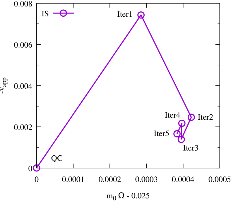
Figure 7: Same as Fig. 2 but for the IS family. All the models are labeled.

Required corrections to the orbital parameters are presented in Fig. 7. They also exhibit similarity with those for the ZS family shown in Fig. 2. The situation should change, however, if we further reduce the eccentricity to, say, $e\lesssim${10}^{-4}$$, where precession-induced modulation is likely to play a role Buonanno et al. (2011).

To monitor the eccentricity using $\Psi_{4}$, the mode mixing due to the precession has to be removed appropriately. Because our simulations adopt the direction of the total angular momentum as the $z$ axis, the precession-induced modulation is likely minimal but definitely non-negligible O’Shaughnessy et al. (2011); Schmidt et al. (2012). In this paper, we transform $\Psi_{4}$ obtained in our simulations to components in the coprecessing frame defined according to Refs. O’Shaughnessy et al. (2011); Boyle et al. (2011); Ochsner and O’Shaughnessy (2012) restricting ourselves only to $l=2$ modes. To our knowledge, this is the first application of the radiation axis defined in Ref. O’Shaughnessy et al. (2011) to black hole–neutron star binaries in numerical relativity (see also Ref. Kawaguchi et al. (2017) for another choice of the radiation axis Schmidt et al. (2011)).

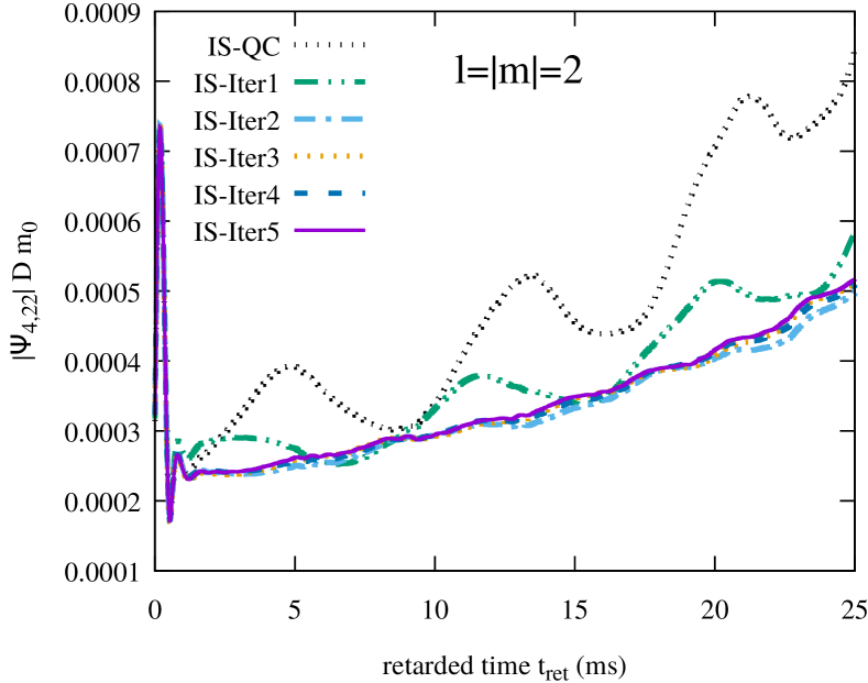
Figure 8: Same as Fig. 4 but for the average of the amplitudes of $l=m=2$ and $l=-m=2$ modes of the IS family.

Time evolution of the $l=|m|=2$ mode amplitude of $\Psi_{4}$ is shown in Fig. 8. Specifically, we average the amplitudes of $m=2$ and $m=-2$ modes to remove reflection-asymmetric components Pekowsky et al. (2013); Boyle et al. (2014). Overall, we confirm that the reduction of eccentricity is not a gauge artifact. Although the evolution appears similar to that of the ZS model as expected from the approximate absence of the spin component along the orbital angular momentum, definite comparisons are difficult because of the presence of additional structures in $\Psi_{4}$ of the IS model. In particular, modulation with approximately twice the orbital frequency, which is consistent with the precession-induced one, appears to be present in our coprecessing-frame data. We defer detailed investigations of this feature to a future task.

III.2.2 Properties of initial data

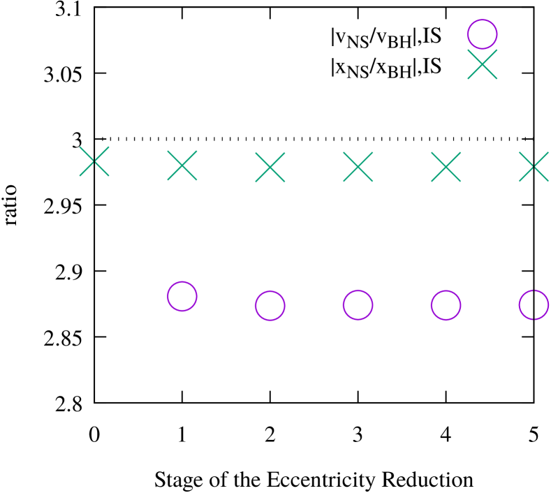
Figure 9: Same as Fig. 5 but for the IS family. Note the different vertical scale.

The binding energy and the orbital angular momentum of the IS family are shown in Table 2. They again behave similarly to those of the ZS family. Post-Newtonian predictions are $|M_{0}-m_{0}|=0.0393M_{\odot}$ and $L_{0}=21.63M_{\odot}^{2}$ for $m_{0}\Omega=0.025$, and they change to $|M_{0}-m_{0}|=0.0397M_{\odot}$ and $L_{0}=21.56M_{\odot}^{2}$ for $m_{0}\Omega=0.0253833$ corresponding to IS-Iter5. The level of agreement and its improvement are similar to those for the ZS model.

The amount of junk radiation is different between the ZS and IS models. The junk radiation carries away the energy $\Delta E\sim$2\text{\times}{10}^{-3}$M_{\odot}$ and the angular momentum $\Delta L\sim 5$–$$6\text{\times}{10}^{-2}$M_{\odot}^{2}$ for the IS model. These values are closer to those for the AS model than for the ZS model because the property of junk radiation is influenced strongly by the magnitude of the black hole spin. While $\Delta E$ corresponds to $\approx 140\%$ of the difference of the binding energy between IS-Iter5 and the post-Newtonian prediction, $\Delta L$ approximately coincides with the difference of the orbital angular momentum. What is common among all the models considered in this study is that a significant fraction of the difference between low-eccentricity initial data and the post-Newtonian prediction may be ascribed to the junk radiation.

We also plot the ratio of the approaching velocity and the $x$ coordinate of the black hole and the neutron star in Fig. 9. They are reasonably close to the expected values of $Q=3$. To sum up, our initial-data computations including the eccentricity reduction perform similarly for both nonprecessing and precessing configurations.

IV Summary

We demonstrated that the orbital eccentricity in black hole–neutron star binaries prepared in the puncture framework can be reduced to $e\lesssim 0.001$ irrespective of the spin configuration. Following previous work Pfeiffer et al. (2007); Buonanno et al. (2011); Kyutoku et al. (2014a), we iteratively modify parameters specifying the initial data, namely the orbital angular velocity and the approaching velocity of the binary, by analyzing orbital evolution derived by dynamical simulations for a few orbits. Because the linear momentum of the black hole cannot be specified freely in our puncture-based formulation for initial data of black hole–neutron star binaries, we cannot adopt methods developed for binary black holes in a straightforward manner Husa et al. (2008); Boyle et al. (2008); Pürrer et al. (2012); Ramos-Buades et al. (2019). In this work, we instead control the approaching velocity of the neutron star by modifying the helical Killing vector required to integrate Euler’s equation Kyutoku et al. (2014a) (see also Ref. Moldenhauer et al. (2014)). The approaching velocity of the black hole is induced automatically by the requirement that the total linear momentum of the system vanishes. To control the approaching velocity of the binary, the velocity of the black hole is defined by the minus of the shift vector at the puncture. Accordingly, we also determine the location of the rotational axis by requiring that the puncture moves in the azimuthal direction with the orbital angular velocity Shibata and Taniguchi (2008).

Our work completes, at least as a first serious attempt, the eccentricity reduction for initial data of compact binaries required for fully exploiting ground-based gravitational-wave detectors Abbott et al. (2019b). For binary neutron stars, essentially the same formulation has been adopted by various authors to reduce the orbital eccentricity Kyutoku et al. (2014a); Moldenhauer et al. (2014); Haas et al. (2016). Although the eccentricity reduction of binary black holes has long been performed both in the excision Pfeiffer et al. (2007) and puncture Pürrer et al. (2012) frameworks, it has been performed only in the former for black hole–neutron star binaries Foucart et al. (2008). Taking the robustness of the moving-puncture simulations into account, our formulation may potentially be advantageous for systematic exploration of a wide parameter space of black hole–neutron star binaries (see Refs. Kyutoku et al. (2010, 2011) for our early effort).

Unsatisfactory aspects of our eccentricity reduction indicate future directions for the improvement. The required number of iterative corrections is generally larger than that for binary neutron stars, particularly for the case that the black hole spin is high. In addition, previous studies on binary black holes in the puncture framework suggest that the gauge dynamics could degrade the accuracy in fitting the orbital motion at $e\lesssim 0.001$ Pürrer et al. (2012). Although the initial transition of the gauge condition could continue to be an obstacle, these features may be improved by adopting a sophisticated fitting procedure Buonanno et al. (2011); Ramos-Buades et al. (2019). Differently from the case of binary neutron stars Kyutoku et al. (2014a), fitting formulas derived from binary-black-hole simulations in the excision framework Mroué and Pfeiffer (2012) do not reduce the orbital eccentricity to a satisfactory level of $e\approx 0.001$. It would be helpful to develop phenomenological formulas tailored to black hole–neutron star binaries in the puncture framework after performing systematic eccentricity reduction. Regarding the low-eccentricity initial data themselves, global quantities like the binding energy and the orbital angular momentum do not agree very well with post-Newtonian predictions. Our investigation suggests that a significant fraction of the deviation may be ascribed to junk radiation, and formulation that suppresses it will improve the accuracy of initial data and dynamical simulations (see also Refs. Foucart et al. (2008); Lovelace et al. (2008) for issues related to the high spin).

Detections of gravitational waves from black hole–neutron star binaries are now becoming realistic. It is probable that we will detect their coalescences with measurable matter effects, possibly associated with electromagnetic counterparts (see, e.g., Refs. Kyutoku et al. (2013, 2015)), in the foreseeable future. We are now systematically performing long-term simulations of inspiraling black hole–neutron star binaries, extending our previous work on binary neutron stars Kiuchi et al. (2017, 2020), to develop reliable gravitational-wave templates. We plan to report results derived by these simulations elsewhere.