A relativistic formalism to compute quasi-equilibrium configurations
of non-synchronized neutron star binaries

Abstract

A general relativistic version of the Euler equation for perfect fluid hydrodynamics is applied to a system of two neutron stars orbiting each other. In the quasi-equilibrium phase of the evolution of this system, a first integral of motion can be derived for certain velocity fields of the neutron star fluid including the (academic) case of co-rotation with respect to the orbital motion (synchronized binaries) and the realistic case of counter-rotation with respect to the orbital motion. The velocity field leading to this latter configuration can be computed by solving three-dimensional vector and scalar Poisson equations.

I Introduction

Considerable efforts by many groups in the world are currently devoted to the computation of the gravitational radiation from binary neutron star coalescences (see e.g. [1] or [2] for recent reviews). These phenomena constitute one of the most promising sources of gravitational radiation for the interferometric detectors GEO600, LIGO and VIRGO currently under construction [3, 4]. Basically two different approaches are used to tackle this problem:

  A1

high-order Post-Newtonian analytical calculations in the point-mass limit for the two coalescing objects (see [2] for a review);

  A2

hydrodynamical numerical simulations which treat the neutron stars as perfect fluid balls. In this latter category, different methods, based on different approximations, can be distinguished:

  A2a

Newtonian affine approximations which consist in modeling the stars by triaxial ellipsoids, thereby reducing the dynamical degrees of freedom of a star to a finite number and leading to ordinary differential equations for the evolution, instead of partial differential equations [5, 6, 7, 8];

  A2b

Post-Newtonian affine approximations, at the 1-PN order [9, 10, 11] or at the 2-PN order [12];

  A2c

Newtonian hydrodynamical simulations, either based on finite difference methods [13, 14, 15, 16, 17] or on the Smooth Particles Hydrodynamical (SPH) method [18, 19, 20, 21] (see ref. [17] for a comparison of various codes);

  A2d

Post-Newtonian (at the order 1-PN) hydrodynamical simulations with a finite difference method [22, 23];

  A2e

fully relativistic hydrodynamical simulations within the 3+1 formalism of general relativity and using the approximation of a conformally flat spatial 3-metric along with no gravitational field dynamics [24, 25, 26, 27, 28] (see also [29]).

The analytical Post-Newtonian approach (A1) allows to compute the evolution of the binary system from an arbitrary early stage, when the separation between the two components is large, up to the rapid inspiral phase driven by the rapid loss of orbital energy by gravitational radiation. This approach breaks down when finite size effects (tidal forces, disruption of one of the stars) become important, i.e. during the coalescence phase. This final stage can be studied only by means of the numerical hydrodynamical methods (A2). But in this case one faces the problem of the initial conditions. Indeed, due to the limitation of computer resources, the initial conditions cannot be set when the separation between the two stars is much larger than their radii: this would require a prohibitive number of time steps for the evolution codes: the time to coalescence increases with the fourth power of the initial separation $a_{0}$ between the two objects. In practice, all the fully hydrodynamical computations listed in (A2) have been performed with $a_{0}$ set to at most a few times the stellar radius $R$: $a_{0}\simeq 5\,R$ in ref. [21], $a_{0}\simeq 4\,R$ in refs. [18],[19], $a_{0}\simeq 3\,R$ in refs. [14],[15],[17], $a_{0}=2\,R$ (!) in ref. [22]. For the calculations employing the affine approximation instead of the full hydrodynamics, the initial separation is taken to be somewhat larger: $a_{0}\simeq 5\,R$ in ref. [9], $a_{0}\simeq 15\,R$ in ref. [12]. Now at such small separations, two effects are important: (i) tidal forces, i.e. the influence of the gravitational field of star 1 (resp. 2) on the internal structure of star 2 (resp. 1), and (ii) general relativity.

Tidal effects have not been taken into account in the computation of the initial conditions of most of the fully hydrodynamical studies listed in (A2), the only exceptions being the works by Nakamura & Oohara [13], Rasio & Shapiro [20] and Baumgarte et al. [26, 27, 28], all in the case of synchronized binaries, i.e. when the stars have zero spin in the frame co-moving with the two centres of mass. However this rotation state is unrealistic. Indeed it can be seen [5, 30] that the neutron star matter shear viscosity is too small and the binary evolution too rapid to lead to a synchronization of the spin periods with the orbital period. In other words, the inspiral of the binary system can be described in terms of perfect fluids and, in first approximation, all the forces acting on the fluid are gradients of some scalar potentials (gravitational force, gravitational radiation reaction force), so that Kelvin’s theorem applies: the circulation of the fluid velocity (with respect to some inertial frame) on any closed contour comoving with the star (e.g. the stellar equator) is conserved. For each star, the circulation around the equator is roughly $C\simeq 2A\omega$ where $A$ is the area of the equatorial cross section of the star and $\omega$ its mean angular velocity with respect to some inertial frame $\cal R$: $\omega=\Omega_{\rm orb}+\Omega_{\rm spin}$ where $\Omega_{\rm orb}$ is the angular orbital velocity of the system with respect to $\cal R$ and $\Omega_{\rm spin}$ is the rotation angular velocity of the star with respect to the co-orbiting frame. Since the variation of $A$ is small during the evolution to the coalescence, the conservation of $C$ is equivalent to the conservation of $\omega$. When the separation is large $\Omega_{\rm orb}$ is negligible and $\omega$ is equal to the rotation rate of the star. When the separation is that of the initial conditions of the numerical computations (A2) ($a\sim 50{\rm\,km}$) $\Omega_{\rm orb}\sim 2\times 10^{3}{\rm\,rad\,s}^{-1}$, which is much larger than $\omega$, except for neutron stars rotating initially at millisecond periods. Consequently, one must have

$$\Omega_{\rm spin}=-\Omega_{\rm orb}\ .$$ (1)

in order to have a constant circulation. We call configurations obeying (1) counter-rotating configurations. They represent realistic initial conditions for neutron star binary coalescence.

Some of the fully hydrodynamical calculations listed in (A2) employ (1) as initial conditions [14, 15, 21]. But none of them take into account the tidal effects: the stars are taken to be either spherical [15, 21] or axisymmetric [14] (as mentioned above, the only computations with self-consistent initial conditions concerns synchronized binaries [13, 20, 26, 27, 28], for which $\Omega_{\rm spin}=0$). To date, the only self-consistent initial conditions obeying (1) have been computed by Bonazzola & Marck [32]. As can be seen in Fig. 3 of ref. [32], the tidal deformation is quite important when the separation is $a_{0}\simeq 3\,R$. However, these initial conditions have not been employed in evolution calculations.

It must be noticed that some of the studies performed in the affine approximation (A2a) make use of self-consistent counter-rotating initial conditions. They correspond to irrotational Darwin-Riemann ellipsoids [6, 8] or (in the approximation of a large separation) irrotational Roche-Riemann ellipsoids [5].

As regards general relativistic effects, the often used Newtonian approximation [items (A2a) and (A2c)] is very crude, in particular for the neutron star internal structure: let us recall that for a typical $1.4\,M_{\odot}$ neutron star, the central value of the metric coefficient $g_{00}$ is around $0.4$, which shows that even a (first order) Post-Newtonian approximation is not sufficient for describing these objects.

The purpose of the present article is to give a method for computing self-consistent (i.e. including the tidal and rotational distortion) and realistic (i.e. obeying (1)) initial conditions for binary neutron stars in the framework of the full general relativity. Therefore, this work can be conceived as the extension to general relativity of Bonazzola & Marck results [32].

The envisaged problem can be decomposed in two parts: (i) the computation of the gravitational field (i.e. the spacetime metric) generated by the two stars and their motion and (ii) the computation of the stellar structure (density distribution, velocity field,…) in that gravitational field. Part (i) is the main topic of numerical relativity and can be, at least in principle, be achieved by means of the classical 3+1 formalism (see e.g. [33] and [34]). This paper focuses on the determination of the stellar structure. For this purpose, we consider that in the vicinity of the searched initial conditions, the system evolves along a sequence of equilibrium states. We obtain a first integral of motion for certain classes of velocity field inside the neutron stars, including the co-rotating and the (realistic) counter-rotating cases.

The plan of the paper is as follows. Sect. II translates the basic assumption of quasi-equilibrium in geometrical terms (a spacetime symmetry) which leads to the definition of a privileged observer (the “co-orbiting” observer). The (relativistic) Euler equation for the fluid velocity is then derived in the frame of that observer (Sect. III). Necessary and sufficient conditions to get a first integral of the Euler equation are given in Sect. IV. This first integral is trivially obtained in the (unrealistic) case of co-rotating stars. The astrophysically relevant case of counter-rotating stars is presented in Sect. V. A method of resolution is discussed in Sect. VI.

II Spacetime symmetry and choice of coordinates

A Quasi-equilibrium hypothesis

When the separation between the centres of the two neutron stars is about $50{\rm\,km}$ (in harmonic coordinates) the time variation of the orbital period, $\dot{P}_{\rm orb}$, computed at the 2-PN order by means of the formulas established by Blanchet et al. [35] is about $2\%$. The evolution at this stage can thus be still considered as a sequence of equilibrium configurations. Moreover the orbits are expected to be circular (vanishing eccentricity), as a consequence of the gravitational radiation reaction [36]. In terms of the spacetime geometry, we translate these assumptions by demanding that there exists a Killing vector field $l^{\alpha}$ which is expressible as

$$l^{\alpha}=k^{\alpha}+\Omega_{\rm orb}\,m^{\alpha}\ ,$$ (2)

where $\Omega_{\rm orb}$ is a constant, to be identified with the orbital angular velocity with respect to a distant inertial observer, and $k^{\alpha}$ and $m^{\alpha}$ are two vector fields with the following properties. $k^{\alpha}$ is timelike at least far from the binary and is normalized so that far from the star it coincides with the 4-velocity of inertial observers. $m^{\alpha}$ is spacelike, has closed orbits, is zero on a two dimensional timelike surface, called the rotation axis, and is normalized so that $\nabla_{\mu}(m_{\rho}m^{\rho})\nabla^{\mu}(m_{\sigma}m^{\sigma})/(4m_{\nu}m^{\nu})$ tends to $1$ on the rotation axis [this latter condition ensures that the parameter $\phi$ associated with $m^{\alpha}$ along its trajectories by $m^{\alpha}=(\partial/\partial\phi)^{\alpha}$ has the standard $2\pi$ periodicity]. Let us call $l^{\alpha}$ the helicoidal Killing vector. We assume that $l^{\alpha}$ is a symmetry generator not only for the spacetime metric $g_{\alpha\beta}$ but also for all the matter fields. In particular, $l^{\alpha}$ is tangent to the world tubes representing the surface of each star, hence its qualification of helicoidal (cf. Figure 1).

The approximation suggested above amounts to neglect outgoing gravitational radiation. For non-axisymmetric systems — as binaries are — it is well known that imposing $l^{\alpha}$ as an exact Killing vector leads to a spacetime which is not asymptotically flat [37]. Thus, in solving for the gravitational field equations, a certain approximation has to be devised in order to avoid the divergence of some metric coefficients at infinity. For instance such an approximation could be the Wilson & Mathews scheme [38] that amounts to solve only for the Hamiltonian and momentum constraint equations. This approximation has been used in all the fully relativistic studies to date [24, 25, 26, 27, 28] and is consistent with the existence of the helicoidal Killing vector field (2). Note also that since the gravitational radiation reaction shows up only at the 2.5-PN order, the helicoidal symmetry is exact up to the 2-PN order.

B 3+1 Foliation of spacetime

For the considered problem, two types of coordinates can be envisaged: “non-rotating” coordinates $(t,x^{i})$ which are Minkowskian at infinity, so that $k^{\alpha}$ is the first vector of the natural basis corresponding to these coordinates and “co-rotating” coordinates $(t^{\prime},x^{i^{\prime}})$ so that $l^{\alpha}$ is the first vector of their natural basis. There is a lot of ways to do this. We choose both coordinate systems so that the hypersurfaces $t={\rm const}$ and $t^{\prime}={\rm const}$ coincides and are maximal spacelike hypersurfaces. More precisely, we suppose that there exists a slicing of spacetime by a family of spacelike hypersurfaces $(\Sigma_{t})$ so that (i) each $\Sigma_{t}$ is spacelike and (ii) $m^{\alpha}$ is tangent to $\Sigma_{t}$.

1 Non-rotating coordinates

On each $\Sigma_{t}$, we choose a system of Cartesian coordinates $x^{i}=(x,y,z)$, such that $(t,x^{i})$ is a system of spacetime coordinates satisfying to

$$k^{\alpha} = \left({\partial\over\partial t}\right)^{\alpha}$$ (3)

$$m^{\alpha} = -y\left({\partial\over\partial x}\right)^{\alpha}+x\left({\partial\over\partial y}\right)^{\alpha}\ .$$ (4)

The lapse function $N$ and shift vector $N^{\alpha}$ associated with these coordinates are defined by

$$k^{\alpha}=Nn^{\alpha}-N^{\alpha}\qquad\mbox{and}\qquad n_{\mu}N^{\mu}=0\ ,$$ (5)

where $n^{\alpha}$ is the future directed unit 4-vector normal to the hypersurface $\Sigma_{t}$.

2 Rotating coordinates

We call rotating coordinates any coordinate system $x^{i^{\prime}}$ on $\Sigma_{t}$ such that $(t^{\prime}=t,x^{i^{\prime}})$ is a spacetime coordinate system satisfying to

$$l^{\alpha}=\left({\partial\over\partial t^{\prime}}\right)^{\alpha}\ .$$ (6)

In other words, the lines $x^{i^{\prime}}={\rm const}$ are the trajectories of $l^{\alpha}$. This latter being a Killing vector, this means that $t^{\prime}$ is an ignorable coordinate for such systems. In numerical studies, we will use these types of coordinates to reduce the a priori 4-D problem to a 3-D one. In practice, three rotating coordinate systems can be used: one centered on each star, to describe properly the hydrodynamics, and a third one centered on the rotation axis, to describe the gravitational field. The lapse function and shift vector associated with rotating coordinates are immediately deduced from Eqs. (2) and (5) which result in

$$l^{\alpha}=Nn^{\alpha}-B^{\alpha}\ ,$$ (7)

with

$$B^{\alpha}:=N^{\alpha}-\Omega_{\rm orb}\,m^{\alpha}\ .$$ (8)

Since $m^{\alpha}$ is parallel to $\Sigma_{t}$, $B^{\alpha}$ is indeed the shift associated with rotating coordinates (cf. Figure 1). Note that rotating and non-rotating coordinates have the same lapse $N$ for they define the same spacetime foliation.

The Killing equation $\nabla_{\alpha}l_{\beta}+\nabla_{\beta}l_{\alpha}=0$, once projected onto $\Sigma_{t}$, leads to the following relation between the extrinsic curvature tensor $K_{\alpha\beta}$ of the hypersurfaces $\Sigma_{t}$ and the derivatives of the shift vector $B^{\alpha}$:

$$2NK_{\alpha\beta}=-\nabla_{\alpha}B_{\beta}-\nabla_{\beta}B_{\alpha}-2n_{\alpha}n_{\beta}n^{\mu}\nabla_{\mu}N$$ (9)

or, equivalently,

$$2NK_{\alpha\beta}=-\hat{\nabla}_{\alpha}B_{\beta}-\hat{\nabla}_{\beta}B_{\alpha}\ ,$$ (10)

where $\hat{\nabla}_{\alpha}$ stands for the covariant derivative associated with the 3-metric $h_{\alpha\beta}$ induced by $g_{\alpha\beta}$ onto the hypersurfaces $\Sigma_{t}$. Note that $K_{\alpha\beta}$ is linked to the covariant derivative of $n^{\alpha}$ by the formula

$$\nabla_{\beta}n_{\alpha}=-K_{\alpha\beta}-\hat{\nabla}_{\alpha}(\ln N)\,n_{\beta}\ .$$ (11)

In the following an extensive use is made of this relation, without explicitly mention it.

C The co-orbiting observer

Let us call the co-orbiting observer the observer $\cal O$ whose world lines coincide with the trajectories of the symmetry group when these latter are timelike, which encompasses the region occupied by the two stars. $\cal O$’s 4-velocity $v^{\alpha}$ can be written:

$$v^{\alpha}=e^{-\Phi}\,l^{\alpha}\ ,$$ (12)

where $\Phi$ is a scalar field which is uniquely specified by the normalization relation $v_{\mu}v^{\mu}=-1$. It can be seen easily that $\Phi$ is related to the lapse $N$, the shift vectors $B^{\alpha}$ and $N^{\alpha}$, the azimuthal vector $m^{\alpha}$ and the orbital angular velocity $\Omega_{\rm orb}$ by

$$e^{2\Phi}=N^{2}-B_{\mu}B^{\mu}=N^{2}-\Omega_{\rm orb}^{2}m_{\mu}m^{\mu}+2\Omega_{\rm orb}m_{\mu}N^{\mu}-N_{\mu}N^{\mu}\ .$$ (13)

Let $q_{\alpha\beta}$ be the projector onto the 3-planes $\Pi$ orthogonal to $v^{\alpha}$:

$$q_{\alpha\beta}:=g_{\alpha\beta}+v_{\alpha}\,v_{\beta}\ .$$ (14)

The kinematics of the observer $\cal O$ is entirely specified by the Ehlers decomposition [39] of the covariant (with respect to $g_{\alpha\beta}$) derivative of $v^{\alpha}$:

$$\nabla_{\beta}v_{\alpha}=\omega_{\alpha\beta}+\theta_{\alpha\beta}-a_{\alpha}v_{\beta}\ ,$$ (15)

where

$$\omega_{\alpha\beta}:=q_{\alpha}^{\ \,\mu}q_{\beta}^{\ \,\nu}\nabla_{[\nu}\,v_{\mu]}$$ (16)

is the rotation 2-form of $\cal O$,

$$\theta_{\alpha\beta}:=q_{\alpha}^{\ \,\mu}q_{\beta}^{\ \,\nu}\nabla_{(\nu}\,v_{\mu)}$$ (17)

is the expansion tensor of $\cal O$ and

$$a_{\alpha}:=v^{\mu}\nabla_{\mu}v_{\alpha}$$ (18)

is the 4-acceleration of $\cal O$. The property (12), namely that $v^{\alpha}$ is collinear to a Killing vector, means that $v^{\alpha}$ is an isometric flow [39] and leads to

$$\theta_{\alpha\beta}=0$$ (19)

and

$$a_{\alpha}=\nabla_{\alpha}\Phi\ .$$ (20)

Equation (19) shows that $v^{\alpha}$ is a rigid flow.

The three-dimensional vector space $\Pi$ represents the local rest frame of $\cal O$. Note that since $\cal O$ is rotating ($\omega_{\alpha\beta}\not=0$, see below), $\Pi$ is not integrable into global 3-surfaces. $q_{\alpha\beta}$ is the (positive definite) metric tensor induced by $g_{\alpha\beta}$ on $\Pi$. We can introduce the alternating tensor within $\Pi$ as

$$\bar{\epsilon}_{\alpha\beta\gamma}:=v^{\mu}\epsilon_{\mu\alpha\beta\gamma}\ ,$$ (21)

where $\epsilon_{\alpha\beta\gamma\delta}$ is the spacetime alternating tensor associated with the spacetime metric $g_{\alpha\beta}$. The rotation 2-form of $\cal O$ is fully specified by its dual within $\Pi$: $\omega_{\alpha\beta}=-\omega^{\mu}\bar{\epsilon}_{\mu\alpha\beta}$, where

$$\omega^{\alpha}:=-{1\over 2}\bar{\epsilon}^{\,\alpha\mu\nu}\omega_{\mu\nu}={1\over 2}\bar{\epsilon}^{\,\alpha\mu\nu}\nabla_{\mu}v_{\nu}\ .$$ (22)

Note that the Raychaudhuri identity for the flow $v^{\alpha}$ reduces to a simple relation between the norm of $\omega^{\alpha}$ and the Laplacian of $\Phi$:

$$\omega_{\mu}\omega^{\mu}=-\nabla_{\mu}\nabla^{\mu}\Phi+{1\over 2}R_{\mu\nu}v^{\mu}v^{\nu}\ ,$$ (23)

where $R_{\alpha\beta}$ is the Ricci tensor of the metric $g_{\alpha\beta}$.

By means of Eqs. (12), (7), (8) and the Killing identity $\nabla_{\alpha}l_{\beta}+\nabla_{\beta}l_{\alpha}=0$, the rotation vector (22) can be expressed as

$$\omega^{\alpha}={e^{-\Phi}\over 2}\,\bar{\epsilon}^{\,\alpha\mu\nu}\left[\Omega_{\rm orb}\nabla_{\mu}m_{\nu}-\nabla_{\mu}N_{\nu}+2(\Omega_{\rm orb}m_{\mu}-N_{\mu})\nabla_{\nu}\ln N\right]\ .$$ (24)

III Relativistic Euler equation in the rotating frame

A Fluid motion

As stated in the introduction, the matter constituting the neutron stars can be considered as a perfect fluid, so that its stress-energy tensor writes

$$T^{\alpha\beta}=(e+p)\,u^{\alpha}u^{\beta}+p\,g^{\alpha\beta}\ .$$ (25)

The fluid 4-velocity $u^{\alpha}$ can be decomposed orthogonally with respect to the rotating observer $\cal O$ as follows:

$$u^{\alpha}=\Gamma(V^{\alpha}+v^{\alpha})\ ,$$ (26)

where $\Gamma$ is the Lorentz factor

$$\Gamma:=-v_{\mu}u^{\mu}\ ,$$ (27)

and $V^{\alpha}$ is the fluid 3-velocity with respect to $\cal O$:

$$V^{\alpha}:={1\over\Gamma}q^{\alpha}_{\ \,\mu}u^{\mu}\ .$$ (28)

$V^{\alpha}$ belongs to $\Pi$ and is the fluid velocity as measured by the observer $\cal O$ (i.e. with respect to $\cal O$’s proper time). As an immediate consequence of $u_{\mu}u^{\mu}=-1$, one has the usual relation between $\Gamma$ and $V^{\alpha}$:

$$\Gamma=(1-V_{\mu}V^{\mu})^{-1/2}\ .$$ (29)

To a very good approximation the (cold) neutron star matter equation of state (hereafter EOS) can be considered as barotropic: $e=e(n)$ and $p=p(n)$ where $n$ is the proper baryon density. It is then worth to introduce the logarithm of the ratio of enthalpy per baryon and the baryon mean rest mass $m_{B}$ by

$$H:=\ln\left({e+p\over m_{\rm B}n}\right)\ ,$$ (30)

which we call the log-enthalpy, to re-express $(\nabla_{\alpha}p)/(e+p)$ as a gradient of a scalar: indeed, by virtue of the First Law of Thermodynamics, the following identity holds for any barotropic EOS:

$${\nabla_{\alpha}p\over e+p}=\nabla_{\alpha}H\ .$$ (31)

Then the fundamental energy-momentum conservation equation

$$\nabla_{\mu}T^{\mu\alpha}=0$$ (32)

can easily be shown to be equivalent to the system of the following two equations

$$\nabla_{\mu}(nu^{\mu})=0$$ (33)

$$u^{\mu}\nabla_{\mu}u^{\alpha}+\nabla^{\alpha}H+u^{\mu}\nabla_{\mu}H\,u^{\alpha}=0\ .$$ (34)

Note that Eq. (34) is nothing but the uniformly canonical equation of motion for a single-constituent perfect fluid as given by Carter [40].

B Baryon number conservation

Inserting Eq. (26) into the baryon number conservation equation (33) and using the fact that $v^{\alpha}$ is divergence-free [Eq. (19)] leads to

$$\nabla_{\mu}V^{\mu}+V^{\mu}\nabla_{\mu}\ln(n\Gamma)=0\ .$$ (35)

C Momentum conservation

By projecting Eq. (34) onto $v^{\alpha}$ (i.e. along the world lines of the co-orbiting observer $\cal O$), one obtains the relation

$$V^{\mu}\nabla_{\mu}\left(H+\Phi+\ln\Gamma\right)=0\ ,$$ (36)

which can be considered as a relativistic generalization of the classical Bernouilli theorem, for it means that the quantity $H+\Phi+\ln\Gamma$ is constant along the fluid lines.

By projecting Eq. (34) perpendicularly to $v^{\alpha}$ (i.e. onto the local rest frame of the co-orbiting observer $\cal O$), one obtains the relativistic version of the Euler equation for the fluid velocity with respect to $\cal O$ :

$$V^{\mu}\nabla_{\mu}V^{\alpha}+2\bar{\epsilon}^{\,\alpha}_{\ \ \mu\nu}\omega^{\mu}V^{\nu}+\nabla^{\alpha}\Phi-V^{\mu}\nabla_{\mu}\Phi\ V^{\alpha}+\Gamma^{-2}\nabla^{\alpha}H=0\ .$$ (37)

At the Newtonian limit, the $V^{\mu}\nabla_{\mu}V^{\alpha}$ gives the classical term $(\vec{V}\cdot\vec{\nabla})\vec{V}$ and $2\bar{\epsilon}^{\,\alpha}_{\ \ \mu\nu}\omega^{\mu}V^{\nu}$ gives the Coriolis term $2\,\vec{\omega}\times\vec{V}$, induced by the rotation of the observer $\cal O$ with respect to some inertial frame. The term $\nabla^{\alpha}H$ gives the classical pressure term. Finally $\Phi$ reduces to the sum of the gravitational and centrifugal potentials [cf. Eq. (13)]

$$\Phi\stackrel{{\scriptstyle{\rm Newt.}}}{{\longrightarrow}}\Phi_{\rm grav}-{1\over 2}\left(\vec{\Omega}_{\rm orb}\times\vec{r}\right)^{2}\ ,$$ (38)

$\Phi_{\rm grav}$ being defined so that the gravitational field writes $\vec{g}=-\vec{\nabla}\Phi_{\rm grav}$.

In order to exhibit from Eq. (37) a first integral of motion, we shall write as much terms as possible under the form of gradients. First, it can be seen easily that, similarly to the usual flat space formula, the following identity holds

$$V^{\mu}\nabla_{\mu}V^{\alpha}=\bar{\epsilon}^{\,\alpha}_{\ \ \mu\nu}(\nabla\wedge V)^{\mu}V^{\nu}+\nabla^{\alpha}\left({1\over 2}V_{\mu}V^{\mu}\right)\ ,$$ (39)

where we have introduced the curl of $V^{\alpha}$ within the 3-space $\Pi$:

$$(\nabla\wedge V)^{\alpha}:=\bar{\epsilon}^{\,\alpha}_{\ \ \mu\nu}\nabla^{\mu}V^{\nu}\ .$$ (40)

Putting Eq. (39) into Eq. (37) and performing slight rearrangements results in

$$\nabla_{\alpha}(H+\Phi+\ln\Gamma)+\Gamma^{2}\left\{\bar{\epsilon}_{\alpha\mu\nu}\left[(\nabla\wedge V)^{\mu}+2\omega^{\mu}\right]V^{\nu}+V_{\mu}V^{\mu}P_{\alpha}^{\,\ \nu}\nabla_{\nu}\Phi\right\}=0\ ,$$ (41)

where

$$P_{\alpha}^{\,\ \beta}:=q_{\alpha}^{\,\ \beta}-{V_{\alpha}V^{\beta}\over V_{\mu}V^{\mu}}$$ (42)

is the projector onto the 2-space orthogonal to $V^{\alpha}$, i.e. orthogonal to the fluid lines with respect to $\cal O$. Note that in the case where the fluid is at rest with respect to $\cal O$, $P_{\alpha}^{\,\ \beta}$ is not defined; however, the product $V_{\mu}V^{\mu}P_{\alpha}^{\,\ \beta}$ which appears in Eq. (41) remains well defined and is equal to zero. In the derivation of Eq. (41), use has been made of Eq. (29) to replace the term $\nabla_{\alpha}(V_{\mu}V^{\mu}/2)$ coming from Eq. (39) by $\Gamma^{-2}\nabla_{\alpha}\ln\Gamma$.

D Number of independent components

From the fundamental equation $\nabla_{\mu}T^{\mu\alpha}=0$, which has a priori four independent components, we have derived two scalar equations [Eqs. (35) and Eqs. (36)] and one vectorial equation [Eq. (41)]. Equations (36) and (41) are not independent: the former is a direct consequence of the latter, as seen easily by projecting (41) along $V^{\alpha}$. Moreover, from its construction, (41) has only three independent components for it lies into the 3-planes $\Pi$ orthogonal to $v^{\alpha}$.

We will take the scalar equation (35) and the vectorial equation lying in $\Pi$ (41) as the fundamental equations to be satisfied for our problem.

IV Constraint on the velocity field and first integral of motion

The only assumption underlying Eq. (41) is that the observer $\cal O$, with respect to which the fluid velocity $V^{\alpha}$ is defined, has world lines parallel to the helicoidal Killing vector $l^{\alpha}$. Equation (41) is equivalent to the system

$$\bar{\epsilon}_{\alpha\mu\nu}\left[(\nabla\wedge V)^{\mu}+2\omega^{\mu}\right]V^{\nu}+V_{\mu}V^{\mu}P_{\alpha}^{\,\ \nu}\nabla_{\nu}\Phi=\Gamma^{-2}\nabla_{\alpha}G$$ (43)

$$H+\Phi+\ln\Gamma+G={\rm const.}\ ,$$ (44)

where $G$ is a scalar field defined at least in the stars’ world tubes. The relation (44) constitutes a first integral of motion of the system.

A The co-rotating case

Equation (43) is trivially satisfied in the case $V^{\alpha}=0$ by taking $G={\rm const}$. The first integral of motion reduces then to

$$H+\Phi={\rm const.}$$ (45)

This case is the co-rotating one ($\Omega_{\rm spin}=0$) mentioned in the introduction; it corresponds to synchronized binaries, which are not expected to represent realistic close neutron star binaries, as discussed in Sect. I.

The first integral (45) follows directly from the fact that in the co-rotating case the fluid 4-velocity is parallel to a Killing vector [41]: $V^{\alpha}=0$ is indeed equivalent to $u^{\alpha}=v^{\alpha}=e^{-\Phi}l^{\alpha}$ [cf. Eq. (26)]. The integral (45) is well known in the case of a single rigidly rotating star (see e.g. [42]). For the problem of the initial conditions of a binary coalescence, it has been used by Nakamura & Oohara [13] (at the Newtonian approximation) and Baumgarte et al. [26, 27, 28].

B Formulation of the problem in the general case

From now on, we suppose that $V^{\alpha}\not=0$. By performing the vector product (with respect to $\bar{\epsilon}_{\alpha\beta\gamma}$) of Eq. (43) by $V^{\alpha}$, one can see easily that Eq. (43) is equivalent to the system

$$V^{\mu}\nabla_{\mu}G=0$$ (46)

$$(\nabla\wedge V)^{\alpha}=-2\omega^{\alpha}-\bar{\epsilon}^{\,\alpha\mu\nu}V_{\mu}\nabla_{\nu}\Phi+(\Gamma^{2}V_{\sigma}V^{\sigma})^{-1}\bar{\epsilon}^{\,\alpha\mu\nu}V_{\mu}\nabla_{\nu}G+F\,V^{\alpha}\ ,$$ (47)

where

$$F:={1\over V_{\nu}V^{\nu}}V_{\mu}\left[(\nabla\wedge V)^{\mu}+2\omega^{\mu}\right]\ .$$ (48)

The gravitational field being given, the problem of getting a solution amounts to finding a vector field $V^{\alpha}$ and a scalar field $G$ such that the equations (35), (46) and (47) are satisfied. In Eq. (35), the scalar field $n$ is that related to the gravitational field, $V$ and $G$ by the first integral (44) via the EOS $n=n(H)$. More precisely, let us consider an iterative method for solving this problem. Let us suppose that at a given step, the gravitational field equations have been solved; the potential $\Phi$ and the rotation vector $\omega^{\alpha}$ are then known. The enthalpy $H$ can be then deduced from the first integral (44), by taking for $\Gamma$ and $G$ the values at the previous step or making some extrapolation from a few previous steps. The baryon density $n$ is computed from $H$ by means of the EOS. The system of equations (35), (46) and (47) is then to be solved in $V^{\alpha}$ and $G$. It is however not obvious that a solution exists in the general case. What can be said is that in the Newtonian and incompressible case, solutions do exist and are constituted by S-type Darwin-Riemann ellipsoids [43].

V The counter-rotating case

A Definition

Let us focus on the interesting case of counter-rotating binaries. The concept of counter-rotation has to be defined in the relativistic framework. We shall define it by requiring $V^{\alpha}\not=0$ and the scalar field $G$ introduced in Eqs. (43)-(44) to be constant:

$$G={\rm const.}$$ (49)

This definition is motivated by the fact that at the Newtonian limit it implies $1/2\,(\nabla\wedge V)^{\alpha}=-\omega^{\alpha}$, which is the definition (1) of counter-rotation [cf Eq. (24)].

With the choice (49), Eq. (46) is trivially satisfied and Eq. (47) becomes

$$(\nabla\wedge V)^{\alpha}=-2\omega^{\alpha}-\bar{\epsilon}^{\,\alpha\mu\nu}V_{\mu}\nabla_{\nu}\Phi+F\,V^{\alpha}\ .$$ (50)

B 3+1 decomposition

From the numerical point of view, it is desirable to reduce the problem to the resolution of three-dimensional equations. Now Eq. (50) involves 4-vectors: even if $V^{\alpha}$ is spacelike and belongs to 3-planes orthogonal to $v^{\alpha}$, due to the rotation of this latter, there exists no coordinate system in which $V^{\alpha}$ would have only three non-vanishing components. Therefore, we choose to recast Eq. (50) according to the 3+1 foliation of spacetime introduced in Sect. II B. In this manner, we will consider only 3-vectors belonging to the spacelike hypersurfaces $\Sigma_{t}$. The first step is to introduce the orthogonal decomposition with respect to $\Sigma_{t}$ of the fluid velocity $V^{\alpha}$ with respect to the co-orbiting observer:

$$V^{\alpha}=W^{\alpha}+Zn^{\alpha}\ ,$$ (51)

where

$$W^{\alpha}=h^{\alpha}_{\ \,\mu}V^{\mu}\qquad\mbox{and}\qquad Z=-n_{\mu}V^{\mu}\ ,$$ (52)

where $h_{\alpha\beta}:=g_{\alpha\beta}+n_{\alpha}\,n_{\beta}$ is the orthogonal projector onto $\Sigma_{t}$, or equivalently, the 3-metric induced by $g_{\alpha\beta}$ in $\Sigma_{t}$. Due to the orthogonality relation $v_{\mu}V^{\mu}=0$, the scalar $Z$ is not independent from $W^{\alpha}$: by inserting Eqs. (12) and (7) into $v_{\mu}V^{\mu}=0$, one gets

$$Z=-{1\over N}B_{\mu}W^{\mu}=-{1\over N}B_{i}W^{i}\ .$$ (53)

In the last part of this equation, we have introduced Latin indices, which range from 1 to 3, whereas the Greek indices range from 0 to 3. We will systematically do this in the following for all the tensor fields that lie in $\Sigma_{t}$, such the vectors $B^{\alpha}$ and $W^{\alpha}$. In this way the three-dimensional character of the equations will clearly appear.

The curl on the left-hand side of Eq. (50) is defined within respect to the alternating tensor $\bar{\epsilon}^{\alpha\beta\gamma}$, which is neither parallel nor orthogonal to the $(\Sigma_{t})$ foliation. Let us introduce instead the alternating tensor $\hat{\epsilon}^{\alpha\beta\gamma}$ within the space $(\Sigma_{t},\,h_{\alpha\beta})$ by

$$\hat{\epsilon}^{\alpha\beta\gamma}:=n_{\mu}\epsilon^{\mu\alpha\beta\gamma}\ .$$ (54)

Inserting the identity $\epsilon^{\alpha\beta\gamma\delta}=-4n^{[\alpha}\hat{\epsilon}^{\beta\gamma\delta]}$ into the definition (21) of $\bar{\epsilon}^{\alpha\beta\gamma}$, we arrive at the following expression of $\bar{\epsilon}^{\alpha\beta\gamma}$ in term of $\hat{\epsilon}^{\alpha\beta\gamma}$:

$$\bar{\epsilon}^{\alpha\beta\gamma}=e^{-\Phi}(N\hat{\epsilon}^{\alpha\beta\gamma}-n^{\alpha}B_{\mu}\hat{\epsilon}^{\mu\beta\gamma}-n^{\beta}B_{\mu}\hat{\epsilon}^{\mu\gamma\alpha}-n^{\gamma}B_{\mu}\hat{\epsilon}^{\mu\alpha\beta})\ .$$ (55)

Besides, we can express the four-dimensional covariant derivative of $V^{\alpha}$ which appears in the curl of $V^{\alpha}$ in terms of the three-dimensional covariant derivative of $W^{\alpha}$ with respect to $h_{\alpha\beta}$ :

$$\nabla_{\alpha}V_{\beta}=\hat{\nabla}_{\alpha}W_{\beta}-n_{\alpha}n^{\mu}\nabla_{\mu}W_{\beta}-K_{\alpha\mu}W^{\mu}n_{\beta}+n_{\beta}\nabla_{\alpha}Z-ZK_{\alpha\beta}-Zn_{\alpha}\hat{\nabla}_{\beta}\ln N\ .$$ (56)

A useful formula is that which gives the derivative along $n^{\alpha}$ of any tensor field $X^{\alpha}$ (i) which lies in $\Sigma_{t}$ and (ii) which respects the heloicoidal symmetry (i.e. ${\cal L}_{\bf l}X^{\alpha}=0$):

$$n^{\mu}\nabla_{\mu}X^{\alpha}={1\over N}\left(B^{\mu}\nabla_{\mu}X^{\alpha}-X^{\mu}\nabla_{\mu}B^{\alpha}\right)-K^{\alpha}_{\ \,\mu}X^{\mu}+{X^{\mu}\over N}\hat{\nabla}_{\mu}N\,n^{\alpha}\ .$$ (57)

This formula can be used to express the derivative of $W^{\alpha}$ along $n^{\alpha}$ which appear in the right-hand side of Eq. (56). We can also apply it to $B^{\alpha}$ and get

$$n^{\mu}\nabla_{\mu}B^{\alpha}=-K^{\alpha}_{\ \,\mu}B^{\mu}+{B^{\mu}\over N}\hat{\nabla}_{\mu}N\,n^{\alpha}\ .$$ (58)

By combining Eqs. (40), (56), (55) and (57), we arrive at the 3+1 decomposition of $(\nabla\wedge V)^{\alpha}$:

$$(\nabla\wedge V)^{\alpha} = e^{-\Phi}\hat{\epsilon}^{\alpha\mu\nu}\left[N\hat{\nabla}_{\mu}W_{\nu}+{B_{\mu}\over N}\left(B^{\sigma}\hat{\nabla}_{\sigma}W_{\nu}-W^{\sigma}\hat{\nabla}_{\sigma}B_{\nu}\right)-Z{B_{\mu}\over N}\hat{\nabla}_{\nu}N+B_{\nu}\hat{\nabla}_{\mu}Z-2K_{\mu}^{\ \,\sigma}W_{\sigma}B_{\nu}\right]$$ (60)

$$-e^{-\Phi}\ n^{\alpha}\ \hat{\epsilon}^{\lambda\mu\nu}B_{\lambda}\hat{\nabla}_{\mu}W_{\nu}\ .$$

The term with $\hat{\epsilon}^{\alpha\mu\nu}$ in factor is parallel to the hypersurface $\Sigma_{t}$ (because $\hat{\epsilon}^{\alpha\mu\nu}$ is), whereas the second term is along $n^{\alpha}$.

Similarly Eqs. (22), (12), (7), (55) and (58) leads to the 3+1 splitting of the rotation vector $\omega^{\alpha}$:

$$\omega^{\alpha}=e^{-2\Phi}\,\hat{\epsilon}^{\alpha\mu\nu}\left[-{N\over 2}\hat{\nabla}_{\mu}B_{\nu}-B_{\mu}\hat{\nabla}_{\nu}N+K_{\mu}^{\ \,\sigma}B_{\sigma}B_{\nu}\right]+{e^{-2\Phi}\over 2}\,n^{\alpha}\,\hat{\epsilon}^{\lambda\mu\nu}B_{\lambda}\hat{\nabla}_{\mu}B_{\nu}.$$ (61)

We also need to perform the 3+1 decomposition of the second term on the right-hand side of Eq. (50). The result is

$$\bar{\epsilon}^{\alpha\mu\nu}V_{\mu}\nabla_{\nu}\Phi=e^{-\Phi}\,\hat{\epsilon}^{\alpha\mu\nu}\left[NW_{\mu}\hat{\nabla}_{\nu}\Phi+ZB_{\mu}\hat{\nabla}_{\nu}\Phi-{B^{\sigma}\over N}\hat{\nabla}_{\sigma}\Phi\,W_{\mu}B_{\nu}\right]-e^{-\Phi}\,n_{\alpha}\,\hat{\epsilon}^{\lambda\mu\nu}B_{\lambda}W_{\mu}\hat{\nabla}_{\nu}\Phi\ .$$ (62)

Thanks to Eqs. (60), (61) and (62), the orthogonal projection of Eq. (50) onto the hypersurfaces $\Sigma_{t}$ is straightforward and leads to the three-dimensional equation

$$\hat{\epsilon}^{ijk}\left[N\hat{\nabla}_{j}W_{k}+{B_{j}\over N}\left(B^{l}\hat{\nabla}_{l}W_{k}-W^{l}\hat{\nabla}_{l}B_{k}\right)-Z{B_{j}\over N}\hat{\nabla}_{k}N+B_{k}\hat{\nabla}_{j}Z-2K_{j}^{\ \,l}\,W_{l}B_{k}\right]=$$ (63)

$$\quad\hat{\epsilon}^{ijk}\left[e^{-\Phi}\left(N\hat{\nabla}_{j}B_{k}+2B_{j}\hat{\nabla}_{k}N-2K_{j}^{\ \,l}\,B_{l}B_{k}\right)-NW_{j}\hat{\nabla}_{k}\Phi-ZB_{j}\hat{\nabla}_{k}\Phi+{1\over N}W_{j}B_{k}B^{l}\hat{\nabla}_{l}\Phi\right]+e^{\Phi}\,F\,W^{i}\ .$$ (64)

The baryon number conservation equation (35), once recast in terms of three-dimensional quantities with the help of Eq. (56), writes

$$\hat{\nabla}_{i}W^{i}+W^{i}\hat{\nabla}_{i}\ln(N\Gamma n)+{Z\over N}B^{i}\hat{\nabla}_{i}\ln(Z\Gamma n)=0\ .$$ (65)

A boundary condition on $W^{i}$ can be derived by multiplying this equation by $n$ and setting $n=0$ (definition of the star’s surface) into the result. One obtains, using Eq. (53),

$$\left.\left(W^{i}-{B^{i}B_{j}W^{j}\over N^{2}}\right)\hat{\nabla}_{i}\,n\right|_{\rm surface}=0\ .$$ (66)

The equations to be solved are the three-dimensional vector equation (64) and the scalar equation (65), altogether with the boundary condition (66). Note that once Eq. (64) is satisfied, the other part of the four-dimensional equation (50), namely the part along $n^{\alpha}$, is automatically fulfilled. Indeed, the projection of Eq. (50) along $n^{\alpha}$ leads to [cf. Eqs. (60), (61), (62) and (53)]

$$\hat{\epsilon}^{ijk}B_{i}\hat{\nabla}_{j}W_{k}=e^{-\Phi}\hat{\epsilon}^{ijk}B_{i}\hat{\nabla}_{j}B_{k}-\hat{\epsilon}^{ijk}B_{i}W_{j}\hat{\nabla}_{k}\Phi+{1\over N}B_{i}W^{i}\,F\ ,$$ (67)

which is nothing else than the orthogonal projection of Eq. (64) onto $B^{i}$.

Referring to the discussion in Sect. III D, we conclude that if a 3-vector $W^{i}$ of $\Sigma_{t}$ obeying Eqs. (64) and (65) can be found, the problem is completely resolved. Note that the baryon density $n$ which appears in Eq. (65) is given via the EOS by the log-enthalpy $H$, itself being fully determined (for a fixed gravitational field) by $W^{i}$ via the first integral of motion (44), which becomes in the counter-rotating case

$$H+\Phi+\ln\Gamma={\rm const.}\ ,$$ (68)

where [cf. Eqs. (29) and (51)]

$$\Gamma=(1-W_{i}W^{i}+Z^{2})^{-1/2}\ .$$ (69)

C Formulation in terms of Poisson equations

The equations to be solved, namely Eqs. (64) and (65), can be recast into Poisson equations by looking for solutions under the form

$$W^{i}=\hat{\epsilon}^{ijk}\hat{\nabla}_{j}A_{k}+\hat{\nabla}^{i}\psi\ ,$$ (70)

where $\psi$ is a scalar field and $A^{i}$ is a 3-vector of $\Sigma_{t}$, which without any loss of generality can be taken to be divergence-free :

$$\hat{\nabla}_{i}A^{i}=0\ .$$ (71)

This latter property implies that the curl of $W^{i}$ is related to the Laplacian of $A^{i}$ by

$$\hat{\epsilon}^{ijk}\hat{\nabla}_{j}W_{k}=-\hat{\nabla}_{j}\hat{\nabla}^{j}A^{i}+\hat{R}^{i}_{\ \,j}A^{j}\ ,$$ (72)

where $\hat{R}_{ij}$ is the Ricci tensor of the 3-metric $h_{ij}$ of $\Sigma_{t}$. Inserting Eq. (72) into Eq. (64) leads to the following vector Poisson equation for $A^{i}$:

$$\hat{\nabla}_{j}\hat{\nabla}^{j}A^{i} = \hat{\epsilon}^{ijk}\Bigg{\{}-e^{-\Phi}\left(\hat{\nabla}_{j}B_{k}+2{B_{j}\over N}\hat{\nabla}_{k}N-{2\over N}K_{j}^{\ \,l}\,B_{l}B_{k}\right)+W_{j}\hat{\nabla}_{k}\Phi+{1\over N}\Bigg{[}ZB_{j}\hat{\nabla}_{k}\Phi-{1\over N}W_{j}B_{k}B^{l}\hat{\nabla}_{l}\Phi$$ (74)

$$+{B_{j}\over N}\left(B^{l}\hat{\nabla}_{l}W_{k}-W^{l}\hat{\nabla}_{l}B_{k}\right)-Z{B_{j}\over N}\hat{\nabla}_{k}N+B_{k}\hat{\nabla}_{j}Z-2K_{j}^{\ \,l}\,W_{l}B_{k}\Bigg{]}\Bigg{\}}-{e^{\Phi}\,F\over N}\,W^{i}+\hat{R}^{i}_{\ \,j}A^{j}\ .$$

The divergence of $W^{i}$ evaluated from Eq. (70) is

$$\hat{\nabla}_{i}W^{i}=\hat{\nabla}_{i}\hat{\nabla}^{i}\psi+{1\over 2}\hat{\epsilon}^{ijk}\hat{R}_{klij}A^{l}\ ,$$ (75)

where $\hat{R}_{klij}$ is the Riemann tensor associated with the 3-metric $h_{ij}$. By virtue of the symmetry properties of the Riemann tensor in three dimensions, the last term on the right-hand side of Eq. (75) vanishes identically, so that the divergence of $W^{i}$ is simply the Laplacian of $\psi$ and Eq. (65) becomes

$$\hat{\nabla}_{i}\hat{\nabla}^{i}\psi=-W^{i}\hat{\nabla}_{i}\ln(N\Gamma n)-{Z\over N}B^{i}\hat{\nabla}_{i}\ln(Z\Gamma n)\ .$$ (76)

D Newtonian limit

In the Newtonian limit, $\Phi$ takes the form (38) and $\omega^{\alpha}$ becomes [cf. Eq. (24)]

$$\omega^{\alpha}\stackrel{{\scriptstyle{\rm Newt.}}}{{\longrightarrow}}\vec{\Omega}_{\rm orb}\ .$$ (77)

The rotating-coordinate shift vector $B^{\alpha}$ reduces to $B^{\alpha}=-\Omega_{\rm orb}\,m^{\alpha}$ [cf Eq. (8)], so that Eq. (74) becomes

$$\Delta\vec{A}=2\,\vec{\Omega}_{\rm orb}\ ,$$ (78)

whose divergence-free solution is

$$\vec{A}={1\over 2}\left(\vec{e}_{z}\times\vec{r}\right)^{2}\,\vec{\Omega}_{\rm orb}\ ,$$ (79)

where $\vec{e}_{z}:=\vec{\Omega}_{\rm orb}/\Omega_{\rm orb}$. Finally, Eq. (76) becomes

$$\Delta\psi=-\vec{V}\cdot\vec{\nabla}\ln n\ .$$ (80)

Once this equation is solved, the fluid velocity field with respect to the co-orbiting observer is computed by taking the curl of (79) :

$$\vec{V}=-\vec{\Omega}_{\rm orb}\times\vec{r}+\vec{\nabla}\psi\ .$$ (81)

This is the solution obtained by Bonazzola & Marck [32].

VI Discussion

A Iterative method of resolution

The resolution of the problem amounts to solving the vector Poisson equation (74) for $A^{i}$ and the scalar Poisson equation (76) for $\psi$, with the boundary condition (66) at the surface of each star. These equations involve Laplacian with respect to the curved 3-metric $h_{ij}$, so that even if the right-hand of the equations is supposed to be known (e.g. from a previous step in an iterative method), the numerical solution is not straightforward. A technique which has shown to be successful consists in introducing on $\Sigma_{t}$ a flat 3-metric $\bar{h}_{ij}$ and decomposing the operators into flat-space ordinary Laplacians plus curvature terms [44, 45].

With this technique, the following iterative method can be envisaged to get counter-rotating binary neutron star configurations. The starting point of the procedure can be very crude approximations such as constant density spherical stars with $W^{i}=0$ and a flat spacetime metric. At a given step, the gravitational field equations are to be solved, leading to new values for the functions $N$, $h_{ij}$, $K_{ij}$, $B^{i}$ and $\Phi$ [via. Eq. (13)]. The first integral of motion Eq. (68) yields then to the value of the log-enthalpy $H$ throughout the stars. The Lorentz factor $\Gamma$ which appears in the first integral is to be evaluated by inserting the previous step values of $W^{i}$ in Eq. (69). From $H$ the baryon number density $n$ is computed by means of the EOS and inserted in the right-hand side of the scalar Poisson equation (76). In this right-hand side, as well as in the right-hand side of the vector Poisson equation (74), the value of $W^{i}$ is to be taken from the previous step. This is of course also the case of the functions of $W^{i}$: $Z$ [deduced from $W^{i}$ by Eq. (53)] and $F$ [deduced from $W^{i}$ by Eq. (48)]. The Poisson equations (76) and (74) are then to be solved respectively for $\psi$ and $A^{i}$. The solutions are obtained up to the addition of harmonic functions. These latter are determined in order that the boundary condition (66) is fulfilled. The vector field $W^{i}$ is deduced from the obtained values of $\psi$ and $A^{i}$ via Eq. (70) and a new iteration may begin.

Of course, we do not have any theorem about the convergence of this iterative procedure. All that we can say is that similar schemes have been applied successfully to the computation of axisymmetric [42] and triaxial [41, 45] models of single neutron stars and that in the axisymmetric case, a rigorous proof of convergence has been recently given by Schaudt & Pfister [46].

B Conclusion

Before the inner most stable orbit is reached, the evolution of a binary system of neutron stars can be approximated by a sequence of quasi-equilibrium configurations. For each of these configurations, the spacetime possesses the helicoidal symmetry discussed in Sect. II A. The hydrodynamical part of the problem is then trivial in the case of synchronized binaries, because of the existence of the first integral of motion (45), which means that once the gravitational field is known, the matter distribution in the stars is obtained immediately. However realistic neutron star binaries on the verge of coalescence are not synchronized but rather in counter-rotation. In this case, the velocity field inside the stars with respect to the co-orbiting observer is not zero and has to be computed so that the Euler equation (37) is satisfied. We have presented a formalism which reduces the problem of finding this velocity field to the resolution of three-dimensional scalar and vector Poisson equations. We are currently applying the numerical techniques we have recently developed for solving such equations with spherical-type coordinates [44, 45] in order to get numerical models. We will present the results of this work in a future article.

The formulation presented in this article is independent of any prescription for solving the gravitational field equations (Einstein equations). It simply relies on the assumption of the spacetime helicoidal symmetry and can be used in conjunction with any set of equations for the gravitational field, such as the Wilson & Mathews’ scheme [38, 25] or the 2-PN scheme recently proposed by Asada & Shibata [47]. Note that both schemes involve nothing else but the resolution of Poisson type equations, so that the method that we propose do not require a numerical technique specific to the hydrodynamical equations.

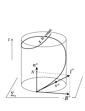
FIG. 1.: Spacetime foliation $\Sigma_{t}$, helicoidal Killing vector $l^{\alpha}$ and its trajectories $x^{i^{\prime}}={\rm const}$, which are the worldlines of the co-orbiting observer (4-velocity: $v^{\alpha}$). Also shown are the rotating-coordinate shift vector $B^{\alpha}$ and the unit future-directed vector $n^{\alpha}$, normal to the spacelike hypersurface $\Sigma_{t}$.

REFERENCES

- [1] S.L. Shapiro, in ref. [3]
- [2] L. Blanchet, in ref. [4] (preprint: gr-qc/9607025)
- [3] I. Ciufolini, F. Fidecaro (eds.), Gravitational Waves: Sources and Detectors, Proc. of the conference held in Cascina (Pisa) (19-23 March 1996), World Scientific, Singapore (1997)
- [4] J.-A. Marck, J.-P. Lasota (eds.), Relativistic Gravitation and Gravitational Radiation, Proc. of Les Houches School (26 September - 6 October 1995), Cambridge University Press, Cambridge, England (1997)
- [5] C.S. Kochanek, Astrophys. J. 398, 234 (1992)
- [6] D. Lai, F.A. Rasio, S.L. Shapiro, Astrophys. J. 420, 811 (1994)
- [7] D. Lai, F.A. Rasio, S.L. Shapiro, Astrophys. J. 437, 742 (1994)
- [8] D. Lai, S.L. Shapiro, Astrophys. J. 443, 705 (1995)
- [9] K.D. Kokkotas, G. Schäfer, Mon. Not. R. Astron. Soc. 275, 301 (1995)
- [10] M. Shibata, K. Taniguchi, Phys. Rev. D 56, 811 (1997)
- [11] J.C. Lombardi, F.A. Rasio, S.L. Shapiro, Phys. Rev. D, in press (preprint: gr-qc/9705128)
- [12] W. Ogawaguchi, Y. Kojima, Prog. Theor. Phys. 96, 901 (1996)
- [13] T. Nakamura, K. Oohara, Prog. Theor. Phys. 86, 73 (1991)
- [14] M. Shibata, T. Nakamura, K. Oohara, Prog. Theor. Phys. 89, 809 (1993)
- [15] M. Ruffert, H.-T. Janka, G. Schäfer, Astron. Astrophys. 311, 532 (1996)
- [16] M. Ruffert, H.-T. Janka, K. Takahashi, G. Schäfer, Astron. Astrophys. 319, 122 (1997)
- [17] M. Ruffert, M. Rampp, H.-T. Janka, Astron. Astrophys. 321, 991 (1997)
- [18] X. Zhuge, J.M. Centrella, S.L.W. McMillan, Phys. Rev. D 50, 6247 (1994)
- [19] X. Zhuge, J.M. Centrella, S.L.W. McMillan, Phys. Rev. D 54, 7261 (1996)
- [20] F. Rasio, S.L. Shapiro, Astrophys. J. 432, 242 (1994)
- [21] M. Davies, W. Benz, T. Piran, F. Thielemann, Astrophys. J. 431, 742 (1994)
- [22] K. Oohara, T. Nakamura, Prog. Theor. Phys. 88, 307 (1992)
- [23] M. Shibata, Phys. Rev. D 55, 6019 (1997)
- [24] J. Wilson, G. Mathews, Phys. Rev. Lett. 75, 4161 (1995)
- [25] J. Wilson, G. Mathews, P. Marronetti, Phys. Rev. D 54, 1317 (1996)
- [26] T.W. Baumgarte, G.B. Cook, M.A. Scheel, S.L. Shapiro, S.A. Teukolsky, Phys. Rev. Lett. 79, 1182 (1997)
- [27] T.W. Baumgarte, S.L. Shapiro, G.B. Cook, M.A. Scheel, S.A. Teukolsky, in Proceedings of the 18th Texas Symposium on Relativistic Astrophysics, eds. Olinto, Frieman and Schramm, World Scientific, Singapore, in press (preprint: gr-qc/9701033)
- [28] T.W. Baumgarte, G.B. Cook, M.A. Scheel, S.L. Shapiro, S.A. Teukolsky, to be published (preprint: gr-qc/9709026)
- [29] K. Oohara, T. Nakamura, in ref. [4]
- [30] L. Bildsten, C. Cutler, Astrophys. J. 400, 175 (1992)
- [31] S.L. Shapiro, Phys. Rev. Lett. 77, 4487 (1996)
- [32] S. Bonazzola, E. Gourgoulhon, P. Haensel, J.-A. Marck, in Approaches to Numerical Relativity, ed. R. d’Inverno, Cambridge University Press, Cambridge, England (1992)
- [33] L. Smarr, J.W. York, Phys. Rev. D 17, 1945 (1978)
- [34] A.M. Abrahams, in ref. [4]
- [35] L. Blanchet, T. Damour, B.R. Iyer, C.M. Will, A.G. Wiseman, Phys. Rev. Lett. 74, 3515 (1995)
- [36] P.C. Peters, Phys. Rev. 136, B1224 (1964)
- [37] J.K. Blackburn, S. Detweiler, Phys. Rev. D 46, 2318 (1992)
- [38] J.R. Wilson, G.J Mathews, in Frontiers in Numerical Relativity, Eds. C.R. Evans, L.S. Finn, D.W. Hobill, Cambridge University Press,Cambridge, England (1989)
- [39] J. Ehlers, Proc. Math. Nat. Sci. Sect. Mainz Academy of Science and Litterature 11, 792 (1961); English translation in Gen. Rel. Grav. 25, 1225 (1993)
- [40] B. Carter, in Active Galactic Nuclei, Eds. C. Hazard & S. Mitton, Cambridge University Press (1979), p. 273
- [41] S. Bonazzola, J. Frieben, E. Gourgoulhon, Astrophys. J. 460, 379 (1996)
- [42] S. Bonazzola, E. Gourgoulhon, M. Salgado, J.-A. Marck, Astron. Astrophys. 278, 421 (1993)
- [43] M.L. Aizenman, Astrophys. J. 153, 511 (1968)
- [44] S. Bonazzola, J. Frieben, E. Gourgoulhon, J.-A. Marck, in ICOSAHOM .95, Proc. Third International Conference on Spectral and High Order Methods, eds. A.V. Ilin & L.R. Scott, Houston Journal of Mathematics, Houston (1996)
- [45] S. Bonazzola, J. Frieben, E. Gourgoulhon, submitted to Astron. Astrophys.
- [46] U.M. Schaudt, H. Pfister, Phys. Rev. Lett. 77, 3284 (1996)
- [47] H. Asada, M. Shibata, Phys. Rev. D 54, 4944 (1996)