New Hyperon Equations of State for Supernovae and Neutron Stars in Density-dependent Hadron Field Theory

Abstract

We develop new hyperon equation of state (EoS) tables for core-collapse supernova simulations and neutron stars. These EoS tables are based on a density-dependent relativistic hadron field theory where baryon-baryon interaction is mediated by mesons, using the parameter set DD2 from Typel et al. (2010) for nucleons. Furthermore, light and heavy nuclei along with the interacting nucleons are treated in the nuclear statistical equilibrium model of Hempel and Schaffner-Bielich which includes excluded volume effects. Of all possible hyperons, we consider only the contribution of $\Lambda$s. We have developed two variants of hyperonic EoS tables: in the np$\Lambda\phi$ case the repulsive hyperon-hyperon interaction mediated by the strange $\phi$ meson is taken into account, and in the np$\Lambda$ case it is not. The EoS tables for the two cases encompass wide range of density ($10^{-12}$ to $\sim$ 1 fm^-3), temperature (0.1 to 158.48 MeV), and proton fraction (0.01 to 0.60). The effects of $\Lambda$ hyperons on thermodynamic quantities such as free energy per baryon, pressure, or entropy per baryon are investigated and found to be significant at higher densities.

The cold, $\beta$-equilibrated EoS (with the crust included self-consistently) results in a 2.1 M_⊙ maximum mass neutron star for the np$\Lambda\phi$ whereas that for the np$\Lambda$ case is 1.95 M_⊙. The np$\Lambda\phi$ EoS represents the first supernova EoS table involving hyperons that is directly compatible with the recently measured 2 M_⊙ neutron stars.

1 Introduction

Compact astrophysical objects are born in the aftermath of massive stars ($>$ 8 M_⊙) through core-collapse supernova (CCSN) explosions in the penultimate stage of their evolution (Bethe, 1990). In the CCSN mechanism, the gravitational collapse of the iron core begins as the core exceeds the Chandrasekhar mass. The subsequent core bounce occurs when the core density reaches beyond normal nuclear matter density and a hydrodynamic shock is generated. If the shock wave is strong enough, this might lead to a prompt supernova explosion, which, however, is not found in recent state-of-the-art computer simulations. The hot and neutrino-trapped protoneutron star (PNS) settles into hydrostatic equilibrium immediately after the core bounce. The PNS could evolve either into a neutron star or into a black hole within a few seconds after the emission of neutrinos. Though the CCSN explosion mechanism has been explored for the past five decades, a complete understanding of this phenomenon is still beyond our reach. In most CCSN simulations, the shock stalls after traveling a few hundred kilometers. The revival of the shock by neutrino heating (Bethe & Wilson, 1985) or the generation of a second shock due to a first order hadron-quark phase transition (Sagert et al., 2009) could trigger a delayed CCSN explosion. Regarding the latter, until now this mechanism was only shown to be working for equations of state (EoS) that are not compatible with the latest neutron star mass measurements such as those from Antoniadis et al. (2013).

Besides the dimensionality of the problem (Nordhaus et al., 2010) and neutrino reaction rates, the EoS of matter plays a tremendous role in a successful CCSN explosion (Janka, 2012). The first nuclear EoS table suitable for CCSN simulations was formulated by Wolff & Hillebrandt (1985) followed by the Lattimer and Swesty (LS) EoS (Lattimer & Swesty, 1991) and the Shen EoS (Shen et al., 1998). The last two EoS tables describe all possible compositions of matter depending on wide ranges of density, temperature, and proton fraction such as free nucleons, light nuclei in coexistence with nucleons, the ideal gas of nuclei, and uniform nuclear matter. The LS EoS table is based on Skyrme interaction for uniform matter and a compressible liquid drop model for non-uniform matter. On the other hand, for the first time, the Shen EoS table was constructed using the relativistic field theory for low- and high-density uniform matter. Non-uniform matter was described by the Thomas-Fermi model. Both of these two approaches, LS and Shen, employed the single nucleus approximation and neglected shell effects. The LS and Shen EoS tables have been used extensively for CCSN simulations over the years.

Recently, several new EoS were developed, keeping in pace with updated knowledge from nuclear structure, experimental data, or neutron star observations, aiming at an improved underlying description and with possibly new particle degrees of freedom taken into account (Hempel & Schaffner-Bielich, 2010; Raduta & Gulminelli, 2010; Shen et al., 2010, 2011a, 2011b; Fischer et al., 2011; Blinnikov et al., 2011; Hempel et al., 2012; Steiner et al., 2013; Fischer et al., 2014; Buyukcizmeci et al., 2013b; Togashi et al., 2014). One such notable nuclear EoS called the HS EoS was formulated within the framework of the nuclear statistical equilibrium (NSE) model (Hempel & Schaffner-Bielich, 2010). The HS EoS table treated the ensemble of nuclei and nucleons in the NSE model using the relativistic mean field model for interacting nucleons, incorporated excluded volume effects in the thermodynamically consistent manner, considered excited states of nuclei and matched the low density matter with uniform matter at high density (Hempel & Schaffner-Bielich, 2010). A new nuclear EoS table was generated adopting the virial expansion for a non-ideal gas of nucleons and nuclei by Shen et al. (2010). The statistical model by Botvina & Mishustin (2004, 2010); Buyukcizmeci et al. (2013b), is based onthe multifragmentation of nuclei in heavy-ion collisions. In Buyukcizmeci et al. (2013a), it was compared with some of the other aforementioned approaches. For the first time, the EoS has been constructed in a variational calculation using bare nuclear forces such as Argonne v18 (AV18) and Urbana IX (UIX) by Togashi et al. (2014); Constantinou et al. (2014), which, however, does not yet include the case of non-uniform matter.

The EoS described above would not only influence the supernova dynamics but also the formation of neutron stars and their structures. Neutron star observations could provide important inputs in the construction of EoS tables for CCSN simulations. The first supernova EoS table directly based on measured masses and radii of neutron stars was developed by Steiner and collaborators (Steiner et al., 2013). Unlike radii, neutron star masses have been estimated to a very high degree of accuracy. This has been possible because post-Keplerian parameters, such as orbital decay, periastron advance, Shapiro delay, and time dilation have been measured in many pulsars. Currently, the accurately measured highest neutron star mass is 2.01$\pm 0.04$ M_⊙ (Antoniadis et al., 2013). This puts a strong constraint on the $\beta$-equilibrated EoS. Most of the nuclear EoS mentioned above result in 2 M_⊙ neutron stars.

Observed neutron star masses are also probes of compositions of dense matter. It has long been debated whether or not novel phases of matter such as hyperons, Bose-Einstein condensates of kaons, and quarks may exist in neutron star interior. It may happen that the phase transition from nuclear matter to exotic matter could occur in the early post-bounce phase of a CCSN. Strange degrees of freedom would be crucial for the long-term evolution of the PNS. It is to be noted that strange matter typically makes the EoS softer resulting in a smaller maximum mass neutron star than that of the nuclear EoS (Glendenning, 2000). van Dalen et al. (2014) showed that the observed high masses of neutron stars in combination with hypernuclear data put tight constraints on the interactions of hyperons in neutron star matter. Note that there is also an interesting interplay between the strangeness content and the symmetry energy on properties of neutron stars, which was recently discussed by Providência (2013) for the case of hyperonic EoS.

Several EoS including quark and hyperon matter were developed for and applied to supernova simulations (Ishizuka et al., 2008; Nakazato et al., 2008; Sagert et al., 2009; Sumiyoshi et al., 2009; Shen et al., 2011c; Nakazato et al., 2012; Oertel et al., 2012; Peres et al., 2013; Banik, 2014). None of the EoS tables with exotic matter were directly compatible with the 2 M_⊙ neutron star or they were just barely acceptable. On the other hand, many model calculations including exotic matter such as hyperons showed that the EoS of $\beta$-equilibrated matter may lead to 2 M_⊙ or more massive neutron stars (Weissenborn et al., 2012a, b; Lastowiecki et al., 2012; Colucci & Sedrakian, 2013; Lopes & Menezes, 2013; Gusakov et al., 2014; van Dalen et al., 2014).

Recently, Fischer et al. (2014) published an quark-hadron hybrid EoS with a maximum mass above 2 M_⊙, which, however, did not lead to a phase-transition-induced explosion. The limited number of realistic supernova EoS with exotic degrees of freedom motivates us to construct a hyperon EoS in the relativistic mean field theory with density-dependent couplings that is compatible with a 2 M_⊙ mass neutron star.

The paper is organized as follows. Section 2 describes the methodology for the calculation of EoS tables including $\Lambda$ hyperons. The results of hyperon EoS tables are discussed in Section 3. Section 4 gives a summary and conclusions. In the Appendix, we give detailed information about the definition of the various quantities stored in the final EoS tables and discuss their accuracy and consistency.

2 Methodology

Here we describe the models to construct the temperature-dependent hyperon EoS spanning over different regimes of baryon number density, temperature, and proton fraction. Compositions of matter vary from one region to the other. Constituents of matter are nuclei, (anti-)neutrons, (anti-)protons, (anti-)$\Lambda$ hyperons, electrons, positrons, and photons. We make the standard assumption that electrons and positrons form a uniform background in this calculation. We do not include the contributions of muons, because in standard core-collapse supernova simulations the net muon lepton fraction is zero. If desired, muons could be added to the EoS as another non-interacting particle species. The contribution of the neutrinos is similarly not taken into account in the EoS. These are typically handled by neutrino transport, because weak equilibrium is generally not obtained. In the following, we discuss various models to compute the EoS of matter in different regimes, where we restrict the discussion on the non-trivial baryonic contribution.

2.1 Density-dependent Relativistic Mean-Field Theory for Baryons

The relativistic mean field (RMF) model with density-dependent couplings is adopted for interacting baryons in this calculation. We exploit this density-dependent RMF model for a transition from non-uniform nuclear to $\Lambda$ hyperon matter. The baryon-baryon interaction in this model is mediated by the exchange of $\sigma$, $\omega$, and $\rho$ mesons. The model may also be extended to include hyperon-hyperon interaction through hidden-strangeness mesons—scalar meson $f_{0}$(975) (denoted hereafter as $\sigma^{*}$) and the vector meson $\phi$(1020) (Schaffner & Mishustin, 1996).

The Lagrangian density (${\cal L}$) of the density-dependent RMF model is given by (Hofmann et al., 2001a, b; Banik & Bandyopadhyay, 2002; Typel et al., 2010),

$${\cal L} = \sum_{F}\bar{\Psi}_{F}\left(i\gamma_{\mu}{\partial^{\mu}}-m_{F}+g_{\sigma F}\sigma-g_{\omega F}\gamma_{\mu}\omega^{\mu}-g_{\rho F}\gamma_{\mu}{\mbox{\boldmath$\tau$}}_{F}\cdot{\mbox{\boldmath$\rho$}}^{\mu}\right)\Psi_{F}$$ (1)

$$+\frac{1}{2}\left(\partial_{\mu}\sigma\partial^{\mu}\sigma-m_{\sigma}^{2}\sigma^{2}\right)-\frac{1}{4}\omega_{\mu\nu}\omega^{\mu\nu}$$

$$+\frac{1}{2}m_{\omega}^{2}\omega_{\mu}\omega^{\mu}-\frac{1}{4}{\mbox{\boldmath$\rho$}}_{\mu\nu}\cdot{\mbox{\boldmath$\rho$}}^{\mu\nu}+\frac{1}{2}m_{\rho}^{2}{\mbox{\boldmath$\rho$}}_{\mu}\cdot{\mbox{\boldmath$\rho$}}^{\mu}+{\cal L}_{YY}~{},$$

where $m_{F}$ is the bare mass of the baryon $F$ and $\tau_{F}$ is the isospin operator. Here $\Psi_{F}$ denotes the isospin multiplets for baryons. In principle, the sum may go over baryon multiplets F = N,$\Lambda$,$\Sigma$,$\Xi$.

The appearance of hyperons depends on the hyperon-nucleon interaction strength in dense matter. The hyperon potential depths in normal nuclear matter are determined from hypernuclei data (Schaffner & Mishustin, 1996; Schaffner & Gal, 2000; Weissenborn et al., 2012a; Oertel et al., 2012). For example, the potential depth of $\Lambda$ hyperons in nuclear matter at the saturation density is obtained from $\Lambda$ hypernuclei data and is found to be attractive. Unlike $\Lambda$ hypernuclei data, $\Sigma$ hypernuclei data as well as $\Xi$ hypernuclei data are scarce. This leads to large uncertainties in estimating the potential depths of $\Sigma$ and $\Xi$ hyperons in nuclear matter. It was noted that $\Sigma$ hypernuclei data indicated a repulsive $\Sigma$ potential depth in nuclear matter (Brat et al., 1999; Schaffner & Gal, 2000). Such a repulsive $\Sigma N$ interaction might rule out the appearance of $\Sigma$ hyperons in dense matter or at least push their onset to very high densities. A few $\Xi$-hypernuclei data gave rise to a less attractive $\Xi$ potential depth in normal nuclear matter than the $\Lambda$ potential depth (Schaffner & Gal, 2000; Weissenborn et al., 2012a; Oertel et al., 2012). Furthermore, $\Lambda$ hyperons, being the lightest hyperons among all hyperons, would be populated first in the system unless the potentials of the others would be very attractive. The appearance of heavier hyperons would be delayed to higher densities. Considering all these facts, we restrict ourselves to nucleons ($N$) and $\Lambda$ hyperons in this calculation. Despite this simplification, the EoS with $\Lambda$s included allows us to study the general features of strange degrees of freedom in core-collapse supernovae. Note that the same implication was used by Peres et al. (2013).

Arguments similar to those given above for the heavier hyperons apply for delta baryons, where it was typically found that these appear, if at all, only at the highest densities in neutron stars (Glendenning, 1985). In addition to the mass, the charge or isospin of hyperons and deltas is also important. It was only recently pointed out by Pagliara et al. (2014) that more modern density functionals that lead to lower symmetry energies at high densities could give an earlier onset of deltas in neutron stars. We leave the interesting aspect of including delta baryons for future study.

The Lagrangian density (${\cal L}_{YY}$) responsible for hyperon-hyperon interaction is given by

$${\cal L}_{YY} = \sum_{F=\Lambda}\bar{\psi}_{F}\left(g_{\sigma^{*}F}\sigma^{*}-g_{\phi F}\gamma_{\mu}\phi^{\mu}\right)\psi_{F}$$ (2)

$$+\frac{1}{2}\left(\partial_{\mu}\sigma^{*}\partial^{\mu}\sigma^{*}-m_{\sigma^{*}}^{2}\sigma^{*2}\right)$$

$$-\frac{1}{4}\phi_{\mu\nu}\phi^{\mu\nu}+\frac{1}{2}m_{\phi}^{2}\phi_{\mu}\phi^{\mu}~{}.$$

The attractive $\Lambda-\Lambda$ interaction is mediated by the exchange of $\sigma^{*}$ meson. However, it is evident from double $\Lambda$ hypernuclei data that this attractive interaction is very weak (Takahashi et al., 2001; Nakazawa et al., 2010; Gal & Millener, 2011). Consequently, we omit the inclusion of $\sigma^{*}$ in Equation (2).

The field strength tensors for vector mesons are given by

$$\omega^{\mu\nu} = \partial^{\mu}\omega^{\nu}-\partial^{\nu}\omega^{\mu}$$

$$\rho^{\mu\nu} = \partial^{\mu}\rho^{\nu}-\partial^{\nu}\rho^{\mu}$$

$$\phi^{\mu\nu} = \partial^{\mu}\phi^{\nu}-\partial^{\nu}\phi^{\mu}.$$

Though the structure of the density-dependent RMF Lagrangian density closely follows that of the RMF model (Shen et al., 1998), there are important differences between those models. In the RMF calculation with density-independent meson-baryon coupling constants, non-linear self interaction terms for scalar and vector fields are inserted to account for higher order density-dependent contributions. However, this is not necessary here as meson-baryon vertices $g_{\alpha F}$, where $\alpha$ denotes the $\sigma$, $\omega$ and $\rho$ fields, are dependent on Lorentz scalar functionals of baryon field operators and adjusted to the Dirac-Brueckner-Hartree-Fock (DBHF) calculations of nuclear matter (Typel & Wolter, 1999; Hofmann et al., 2001a, b).

In mean field approximations adopted here, meson fields are replaced by their expectation values. Only the time-like components of vector fields, and the third isospin component of $\rho$ fields have non-vanishing values in a uniform and static matter. The mean meson fields are denoted by $\sigma$, $\omega_{0}$, $\rho_{03}$, and $\phi_{0}$.

The grand-canonical thermodynamic potential per unit volume of the hadronic phase is given by

$$\frac{\Omega}{V} = \frac{1}{2}m_{\sigma}^{2}\sigma^{2}-\frac{1}{2}m_{\omega}^{2}\omega_{0}^{2}-\frac{1}{2}m_{\rho}^{2}\rho_{03}^{2}-\frac{1}{2}m_{\phi}^{2}\phi_{0}^{2}-\Sigma^{r}\sum_{i=n,p,\Lambda}n_{i}$$ (4)

$$-2T\sum_{i=n,p,\Lambda}\int\frac{d^{3}k}{(2\pi)^{3}}[\mathrm{ln}(1+e^{-\beta(E^{*}-\nu_{i})})+\mathrm{ln}(1+e^{-\beta(E^{*}+\nu_{i})})]~{},$$

where the temperature is defined as $\beta=1/T$ and $E^{*}=\sqrt{(k^{2}+m_{i}^{*2})}$. In the present work, all Fermi-Dirac integrals are solved with the very accurate and efficient methods of Aparicio (1998); Gong et al. (2001), complemented by analytic approximations where these are even more reliable.

The chemical potential of $i$th baryon ($\mu_{i}$) is defined as

$$\mu_{i}=\nu_{i}+\Sigma_{i}^{v},$$ (5)

where $\Sigma_{i}^{v}$ is the vector self-energy and it is given by

$$\Sigma_{i}^{v}=g_{\omega i}\omega_{0}+g_{\rho i}\tau_{3i}\rho_{03}+g_{\phi i}\phi_{0}+\Sigma^{r}~{},$$ (6)

and the rearrangement term has the form

$$\Sigma^{r}=\sum_{i=n,p,\Lambda}[-\frac{\partial g_{\sigma i}}{\partial n_{i}}\sigma n_{i}^{s}+\frac{\partial g_{\omega i}}{\partial n_{i}}\omega_{0}n_{i}+\frac{\partial g_{\rho i}}{\partial n_{i}}\tau_{3i}\rho_{03}n_{i}+\frac{\partial g_{\phi i}}{\partial n_{i}}\phi_{0}n_{i}]~{}.$$ (7)

Similarly, the expression of scalar self energy for $i$th baryon is given by

$$\Sigma_{i}^{s}=g_{\sigma i}\sigma$$ (8)

Now one can define the effective Dirac baryon mass as $m_{i}^{*}=m_{i}-\Sigma_{i}^{s}$.

For our calculations we assume $\mu_{n}=\mu_{\Lambda}$, i.e., that there is equilibrium with respect to strangeness changing reactions. This is justified because of the moderately long dynamic timescales in supernovae in the range of milliseconds, the high temperatures encountered inside the proto-neutron star, and because we expect that the $\Lambda$ hyperon abundance is only significant at high densities, where weak equilibrium is established.

Next we calculate the thermodynamic quantities of the baryonic matter such as the pressure $P=-{\Omega}/V$ and the energy density

$$\epsilon = \frac{1}{2}m_{\sigma}^{2}\sigma^{2}+\frac{1}{2}m_{\omega}^{2}\omega_{0}^{2}+\frac{1}{2}m_{\rho}^{2}\rho_{03}^{2}+\frac{1}{2}m_{\phi}^{2}\phi_{0}^{2}$$ (9)

$$+2\sum_{i=n,p,\Lambda}\int\frac{d^{3}k}{(2\pi)^{3}}E^{*}\left({\frac{1}{e^{\beta(E^{*}-\nu_{i})}+1}}+{\frac{1}{e^{\beta(E^{*}+\nu_{i})}+1}}\right)~{}.$$

Similarly we can compute neutron, proton, and $\Lambda$ number densities which include contributions from both particle and antiparticles (Shen et al., 2011c). The number density of the $i(=n,p,\Lambda$)-th baryon is $n_{i}=2\int\frac{d^{3}k}{(2\pi)^{3}}\left({\frac{1}{e^{\beta(E^{*}-\nu_{i})}+1}}-{\frac{1}{e^{\beta(E^{*}+\nu_{i})}+1}}\right)$. The scalar density for the $i$th baryon ($n_{i}^{s}$) is

$$n_{i}^{s} = 2\int\frac{d^{3}k}{(2\pi)^{3}}\frac{m_{i}^{*}}{E^{*}}\left({\frac{1}{e^{\beta(E^{*}-\nu_{i})}+1}}+{\frac{1}{e^{\beta(E^{*}+\nu_{i})}+1}}\right)~{}.$$ (10)

We can calculate the entropy density using ${s}=\beta\left(\epsilon+P-\sum_{i=n,p,\Lambda}\mu_{i}n_{i}\right)$. The entropy per baryon is given by $S={s}/{n_{B}}$, where $n_{B}$ is the total baryon density i.e., $n_{B}=\sum_{i}n_{i}$.

The density dependence of nucleon-meson couplings was determined by Typel & Wolter (1999); Typel et al. (2010). The functional forms of the density-dependent couplings $g_{\sigma N}$ and $g{\omega N}$ are given by

$$g_{\alpha N}=g_{\alpha N}(n_{0})f_{\alpha}(x)~{},$$

$$f_{\alpha}(n_{B}/n_{0})=a_{\alpha}\frac{1+b_{\alpha}(x+d_{\alpha})^{2}}{1+c_{\alpha}(x+d_{\alpha})^{2}}~{},$$ (11)

where $n_{0}$ is the saturation density, $\alpha=\sigma,\omega$ and $x=n_{B}/n_{0}$. For $\rho$ mesons, we have

$$g_{\rho N}=g_{\rho N}(n_{0})exp{[-a_{\rho}(x-1)]}~{}.$$ (12)

In this work we employ the DD2 parameter set (Typel et al., 2010; Fischer et al., 2014), where the coefficients in Equations (11) and (12), the saturation density, the nucleon-meson couplings at the saturation density, and the mass of $\sigma$ mesons are determined by fitting the properties of finite nuclei such as binding energies, spin-orbit splittings, charge and diffraction radii, surface thickness, and neutron skin. In this fitting, experimental masses are used for the nucleons. In our EoS calculations, we also use the experimentally measured masses of nucleons. The saturation properties of symmetric nuclear matter are obtained as $n_{0}=0.149065$ fm^-3, binding energy per nucleon 16.02 MeV, incompressibility 242.7 MeV, neutron effective Dirac mass $m_{n}^{*}/m_{n}$ = 0.5628, proton effective Dirac mass $m_{p}^{*}/m_{p}$ = 0.5622, and the symmetry energy 31.67 MeV. The value of the parameter corresponding to the density dependence of the symmetry energy at the saturation density is found to be 55.03 MeV. For detailed definitions of these quantities, see e.g., Typel et al. (2013). These nuclear matter properties are consistent with constraints from theoretical calculations of neutron matter, experimental findings and astrophysical observations of neutron stars (Fischer et al., 2014; Lattimer & Lim, 2013). Note that the values that we obtain differ slightly from those previously reported in Typel et al. (2010). Meson-nucleon couplings at the saturation density and masses of baryons and mesons used in the calculation are shown in Tables 1 and LABEL:table2, respectively.

Nucleons do not couple with $\phi$ mesons i.e. $g_{\phi N}=0$. The density-dependent meson-$\Lambda$ hyperon vertices are obtained from the density-dependent meson-nucleon couplings using $\Lambda$-hypernuclei data (Schaffner & Mishustin, 1996) and the SU(6) symmetry of the quark model. In the RMF model, vector meson - hyperon coupling constants were determined from the SU(6) symmetry relations of the quark model (Schaffner & Mishustin, 1996; Dover & Gal, 1985). Similarly, we obtain vector meson - $\Lambda$ hyperon couplings in this model from the SU(6) symmetry relations (Schaffner & Mishustin, 1996)

$$\frac{1}{2}g_{\omega\Lambda}=\frac{1}{3}g_{\omega N},$$

$$g_{\rho\Lambda}=0,$$

$$2g_{\phi\Lambda}=-\frac{2\sqrt{2}}{3}g_{\omega N}~{}.$$ (13)

Next we obtain the scalar meson coupling to $\Lambda$ hyperons ($g_{\sigma\Lambda}$) from the potential depth of $\Lambda$ hyperons in normal nuclear matter. The $\Lambda$ hyperon potential in saturated nuclear matter is obtained from the experimental data of the single particle spectra of $\Lambda$ hypernuclei. In the density-dependent RMF model, the potential depth of $\Lambda$ hyperon in saturated nuclear matter is given by

$$U_{\Lambda}^{N}(n_{0})=g_{\omega\Lambda}\omega_{0}+\Sigma_{N}^{r}-g_{\sigma\Lambda}\sigma_{0}~{}$$ (14)

where $\Sigma_{N}^{r}$ is the contribution of only nucleons in the rearrangement term as given by Equation (7). In this calculation, the value of the $\Lambda$ potential in normal nuclear matter is taken as $U_{\Lambda}(n_{0})=-30$ MeV (Millener et al., 1988; Mares et al., 1995; Schaffner et al., 1992) and the ratio of $g_{\sigma\Lambda}$ and $g_{\sigma N}$ is $R_{\sigma\Lambda}=g_{\sigma\Lambda}/g_{\sigma N}=0.62008$. Note that Lastowiecki et al. (2012) also extended the DD2 parameterization by including hyperons to describe the structures of hybrid stars. However, they used different assumptions, namely, an SU(3) rescaling with an overall factor $R=0.83$ and they considered the whole baryon octet.

2.2 Extended Nuclear Statistical Equilibrium Model

In the widely used nuclear EoS of Shen and collaborators (Shen et al., 1998, 2011c), heavy nuclei were treated in the Thomas-Fermi approach. The other commonly used nuclear EoS of LS (Lattimer & Swesty, 1991) utilizes a liquid-drop description of nuclei and a non-relativistic parameterization of the nucleon interactions. In both approaches the gas of $\alpha$ particles was dealt with the Maxwell-Boltzmann statistics. Heavy nuclei are populated at low temperature and low density. In the LS and Shen EoS, they used the single nucleus approximation for heavy nuclei having an average representative atomic mass and charge in inhomogeneous nuclear matter.

We adopt the extended NSE model of Hempel & Schaffner-Bielich (2010) to describe the matter composed of light and heavy nuclei along with unbound nucleons at low temperatures ($\sim$ 10 MeV) and low densities below the saturation density. The region where heavy nuclear clusters co-exist with nucleons is known as non-uniform or inhomogeneous nuclear matter. In the HS model, nuclei are described as non-relativistic particles using Maxwell-Boltzmann statistics and medium corrections such as internal excitations or Coulomb screening. Excluded volume effects are taken into account, which ensure the dissolution of heavy nuclei at high densities. Interactions among unbound nucleons are described by Equation (1), employing the same parameter set DD2, but not including hyperons. This is justified because the fraction of $\Lambda$ hyperons is negligibly small in low-temperature and -density domains.

Approximately 8000 nuclear species are considered in the extended NSE model of HS. Experimental masses of nuclei ($A\geq 2$) used in the model are taken from the atomic mass table of Audi et al. (2003). For exotic nuclei without measured masses, theoretical nuclear structure calculations within the framework of finite-range droplet model (FRDM) (Möller et al., 1995) are exploited. Note that nuclei beyond the neutron drip line are not considered. By using nuclear mass tables, nuclear shell effects are automatically included into the calculation. This is necessary to obtain the correct low-density limit, e.g. relevant for consistency with recent electron-capture rates (see Juodagalvis et al. (2010)) and with the simulation of the progenitor star, or if one wants to connect to a non-NSE EoS. However, we also point out that the modification of the nuclear shell structure at high densities is not well described by the HS approach. The HS EoS goes beyond the single nucleus approximation (SNA). Regarding a distribution of only heavy nuclei, it is well known that the SNA has only a small effect on thermodynamic quantities (Burrows & Lattimer, 1984). However, here we also include various light nuclei, which together with unbound nucleons dominate the composition of shock-heated matter (Sumiyoshi & Röpke, 2008) and have a non-negligible impact on thermodynamic quantities (Hempel & Schaffner-Bielich, 2010). Note that the results for light nuclei of the HS model are in good agreement with that of the quantum many-body calculation (Hempel et al., 2011) and also qualitatively with experimental data from heavy-ion collisions (Qin et al., 2012).

The thermodynamic quantities such as pressure, energy density, etc., are obtained from the total canonical partition function given by

$$Z(T,V,\{N_{i}\})=Z_{\rm nuc}~{}\prod_{A,Z}Z_{A,Z}~{}Z_{\rm Coul}\;,$$ (15)

with $V$ denoting the volume of the system. One can write down the Helmholtz free energy using the partition function as,

$$F(T,V,\{N_{i}\}) = -T\mathrm{ln}Z$$ (16)

$$= F_{\rm nuc}+\sum_{A,Z}F_{A,Z}+F_{\rm Coul}\;,$$ (17)

where $F_{\rm nuc}$, $F_{\rm Coul}$, $F_{A,Z}$ are the free energies of nucleons, the Coulomb free energy, and the free energy of the nucleus represented by the Maxwell-Boltzmann distribution (Hempel & Schaffner-Bielich, 2010).

After implementing the excluded volume effects in a thermodynamically consistent manner, the number density of the nuclei is given by (Hempel & Schaffner-Bielich, 2010)

$$n_{A,Z}=\kappa~{}g_{A,Z}(T)\left(\frac{M_{A,Z}T}{2\pi}\right)^{3/2}\exp\left(\frac{(A-Z)\mu_{n}^{0}+Z\mu_{p}^{0}-M_{A,Z}-E^{\rm Coul}_{A,Z}-P^{0}_{\rm nuc}V_{A,Z}}{T}\right)\;,$$ (18)

where $\kappa$ is the volume fraction available for nuclei and defined in terms of local number densities and takes values between 0 and 1. It may be worth noting that Equation (18) can be used to derive a modified Saha equation due to excluded volume corrections.

Next one can define the free energy density (Hempel & Schaffner-Bielich, 2010)

$$f = \sum_{A,Z}f_{A,Z}^{0}(T,n_{A,Z})+f_{\rm Coul}(n_{e},n_{A,Z})+\xi f_{\rm nuc}^{0}(T,n^{\prime}_{n},n^{\prime}_{p})-T\sum_{A,Z}n_{A,Z}\mathrm{ln}(\kappa)\;,$$ (19)

where the first term is the contribution of the non-interacting gas of nuclei. Here $f_{\rm Coul}$ is the Coulomb free energy. The free energy density of the interacting nucleons $f_{\rm nuc}^{0}$ is multiplied by the available volume fraction of nucleons $\xi$. The local number densities of neutrons and protons are denoted by $n^{\prime}_{n}$ and $n^{\prime}_{p}$, respectively. The last term, which corresponds to a hard-core repulsion of nuclei, goes to infinity when $\kappa$ approaches zero near saturation density and the uniform matter is formed.

The energy density is given by the following expression (Hempel & Schaffner-Bielich, 2010):

$$\epsilon = \xi\epsilon_{\rm nuc}^{0}(T,n^{\prime}_{n},n^{\prime}_{p})+\sum_{A,Z}\epsilon_{A,Z}^{0}(T,n_{A,Z})+f_{\rm Coul}(n_{e},n_{A,Z})\;,$$ (20)

$$\epsilon_{A,Z}^{0}(T,n_{A,Z}) = n_{A,Z}\left(M_{A,Z}+\frac{3}{2}T+\frac{\partial g}{\partial T}\frac{T^{2}}{g}\right)\;.$$ (21)

Similarly the total pressure becomes

$$P = P_{\rm nuc}^{0}(T,n^{\prime}_{n},n^{\prime}_{p})+\frac{1}{\kappa}\sum_{A,Z}P_{A,Z}^{0}(T,n_{A,Z})+P_{\rm Coul}(n_{e},n_{A,Z})~{},$$ (22)

$$P_{A,Z}^{0}(T,n_{A,Z}) = Tn_{A,Z}~{}.$$ (23)

Note that all quantities above relating to nucleon contributions are calculated with the RMF model (DD2), as described in Section 2.1 and taking into account general Fermi-Dirac statistics. In the original work of Hempel & Schaffner-Bielich (2010), TMA interactions were used instead. Some further changes were made to improve the description of non-uniform matter. Here we briefly list only the relevant ones: for simplicity, nuclei are only considered up to a temperature of 50 MeV, instead of 20 MeV used previously. In the internal partition function of nuclei, $g_{A,Z}(T)$ in Equation (18), which is taken from Fái & Randrup (1982), only excited states up to the binding energy of the corresponding nucleus are included. Our basic idea is that we want to keep the nucleus bound. If no cutoff in the integral for the excited states was used, arbitrarily large excitation energies would contribute to the energy density. The energy and entropy stored in nuclei would increase with increasing temperature to unphysically large values. We found in different applications of the EOS that the usage of the cutoff leads to a more well-balanced behavior. Nevertheless, it is clear that our description of excited states remains on a rather heuristical level.

2.3 Matching Procedure

In principle, the hyperonic EoS as presented in Section 2.1 could be used directly for the description of the unbound baryon contribution (denoted by the subscript “nuc”) in the statistical model that was summarized in Section 2.2. However, because a complete nucleonic supernova EoS table for the parameter set DD2 and as described in Section 2.2 is already publicly available, called HS(DD2) (see Fischer et al. (2014)), here we follow a different strategy. We expect that nuclei will not be present with high abundances at conditions where hyperons can be formed, i.e., at high densities or high temperatures. Therefore, we do not repeat the calculation of the EoS with non-uniform matter distributions including hyperons, but only replace certain parts of the existing table with the new uniform hyperonic EoS using physical criteria specified in the following. In consequence, the new tables never contain a mixture of hyperons and nuclei.

For the merging of the two tables, we follow a standard thermodynamic criterion, namely that the free energy per baryon at fixed $T$, $n_{B}$, and $Y_{p}$ has to be minimized. However, this physical criteria alone could lead to odd transition behaviors, because transitions from one EoS to the other could also be induced by numerical errors. Here, such unphysical transitions are avoided by introducing a minimal hyperon mass fraction of 10^-5, i.e., the hyperon EoS replaces the nucleonic EoS only if it has a lower free energy per baryon and if $X_{\Lambda}>10^{-5}$. Using these two criteria for the merging of the two EoS, we obtain a smooth and continuous transition boundary.

3 Results and Discussion

We compute the hyperon EoS tables using the DD2 parameter set of Table 1. We denote the hyperon EoS table without $\phi$ mesons as BHB$\Lambda$ corresponding to the composition np$\Lambda$ and the hyperon EoS table with $\phi$ mesons as BHB$\Lambda\phi$ for the np$\Lambda\phi$ case. In both cases, the tables are constructed for temperatures $T=0.1$ to $10^{2.2}\simeq 158.49$ MeV and proton fractions $Y_{p}$ = 0.01 to 0.6, whereas baryon densities range from $n_{B}=10^{-12}$ to 1 fm^-3 for the BHB$\Lambda$ and $n_{B}=10^{-12}$ to $10^{1.08}\simeq 1.2$ fm^-3 for the BHB$\Lambda\phi$ tables. We have different density ranges for the two tables (which are also different compared to the original nucleonic HS(DD2) table), because we could not obtain physical solutions at higher values. We adopt a linear grid spacing of 0.01 for $Y_{p}$ and logarithmic grid spacing of 0.04 for $T$ and $n_{B}$. An overview of the two EoS tables is given in Table 3. Before we go into a detailed description of thermodynamic quantities in hyperon EoS tables, we discuss the $\beta$-equilibrated matter relevant for cold neutron stars.

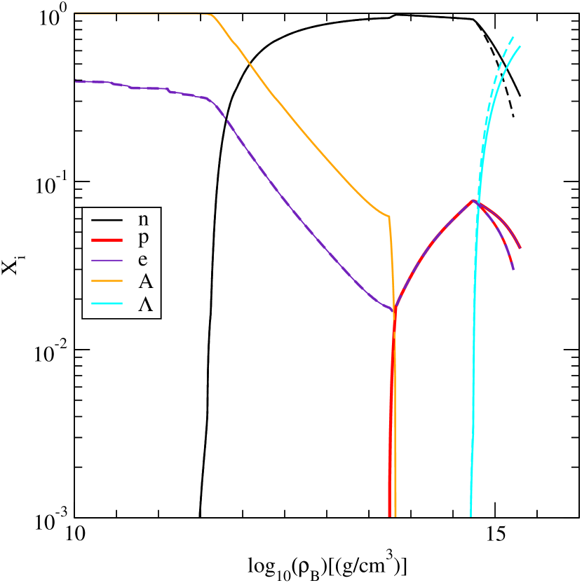
Figure 1: Mass fractions of various species are plotted as a function of baryon mass density with (solid lines) and without (dashed lines) $\phi$ mesons in $\beta$-equilibrated hyperon matter. The curve labeled with “A” shows the mass fraction of heavy nuclei.

We generate the EoS of neutron stars by imposing charge neutrality with the inclusion of electrons and the $\beta$-equilibrium condition without neutrinos into hyperon EoS tables at a very low temperature $T=0.1$ MeV. Fractions of different particle species in $\beta$-equilibrated hyperon matter with and without $\phi$ mesons are plotted as a function of baryon mass density in Figure 1. Here and in the following, we define a “baryon mass density” $\rho_{B}$ by $\rho_{B}=n_{B}\cdot m_{u}$, with the atomic mass unit $m_{u}$. The solid lines represent the npe$\Lambda\phi$ case whereas the dashed lines represent the npe$\Lambda$ case. The beginning of the inner crust is clearly visible by the sudden appearance of free neutrons at a density of $\sim 3\times 10^{11}$ g/cm³. In both cases, heavy nuclei dissolve into their fundamental constituents, i.e., nucleons, below the saturation density and a uniform nuclear matter is formed just after that, marking the transition to the neutron star core. There, proton fractions increase as baryon density increases. The positive charges of protons are balanced by negative charges of electrons. When the baryon density reaches 2.1 $n_{0}$, $\Lambda$ hyperons begin to populate the system in both cases. As the $\Lambda$ fraction rises, neutron and proton fractions drop. Furthermore, it is noted that the $\Lambda$ fraction for the np$\Lambda$ case is higher than that of the np$\Lambda\phi$ case. This may be attributed to the strong repulsive interaction due to $\phi$ mesons at higher densities. This might have a significant impact on the EoS and mass-radius relationship of neutron stars with and without $\phi$ mesons.

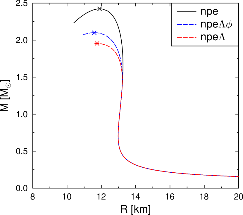
Figure 2: Masses of the neutron star sequence are plotted as a function of radius with (online-version: blue) and without (online-version: red) $\phi$ mesons in hyperon and nucleon matter (solid line), corresponding to the BHB$\Lambda\phi$, BHB$\Lambda$, and HS(DD2) EoS, respectively. Crosses mark the maximum mass configurations.

The mass-radius relationship of the sequence of neutron stars is shown in Figure 2. The solid line represents the nucleons-only neutron star. On the other hand, bold (online-version: blue) and light dashed (online-version: red) lines represent neutron stars including hyperons with and without $\phi$ mesons, respectively. Note that the crust EoS is contained self-consistently, i.e., no external models have to be used. It is evident from Figure 2 that $\Lambda$ hyperons make the EoS softer, resulting in a smaller maximum mass neutron star compared with that of the nucleons-only case. Further, we find that the hyperon-hyperon interaction mediated by $\phi$ mesons makes the hyperon EoS stiffer than the case without $\phi$ mesons. Consequently, the npe$\Lambda\phi$ case has a higher maximum mass than that of the npe$\Lambda$ case because of the repulsive contribution of $\phi$ mesons in the hyperon EoS in the former case. The maximum masses corresponding to the nucleons-only, npe$\Lambda$, and npe$\Lambda\phi$ neutron star sequences are 2.42, 1.95 and 2.10 M_⊙, respectively. We remark that the different extension of the neutron star DD2 EoS with hyperons done previously by Lastowiecki et al. (2012) gave a maximum mass of only 1.94 M_⊙. It is important to note that the maximum mass of npe$\Lambda\phi$ case is well above the benchmark-measured neutron star mass of 2.01$\pm$0.04 M_⊙ (Antoniadis et al., 2013). This is the first supernova EoS with hyperons that is compatible with a 2 M_⊙ neutron star.

We calculate the strangeness fractions $f_{s}$ in maximum mass neutron stars, defined as the ratios of the total numbers of strangeness and the total baryon numbers, and find that in the npe$\Lambda$ case it is 0.071 and in the npe$\Lambda\phi$ case it is 0.059. Using these values we can roughly confirm the empirical relation of Weissenborn et al. (2012b),

$$\frac{M_{\rm max}^{\rm emp}}{M_{\odot}}=\frac{M_{\rm max}(f_{s}=0)}{M_{\odot}}-c(\frac{f_{s}}{0.1})~{},$$ (24)

where $c=0.6$, and that the maximum mass reduces with the strangeness fraction.

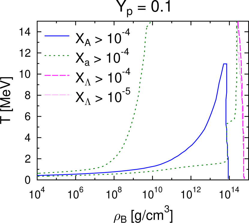
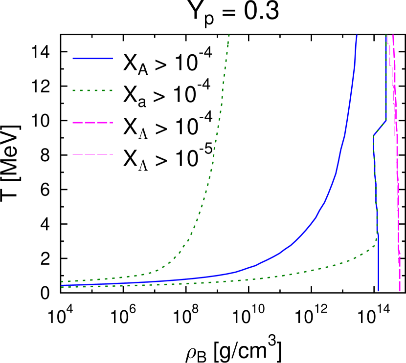
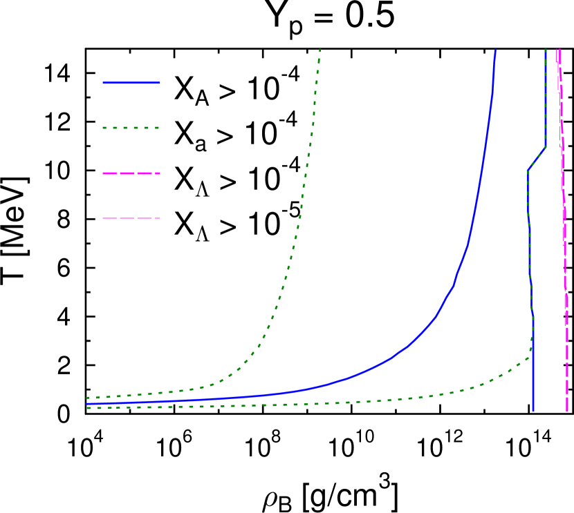
Figure 3: Phase diagrams at $Y_{p}=0.1$, 0.3, and 0.5 (bottom to top) in the $T$-$\rho_{B}$ plane for the BHB$\Lambda\phi$ EoS. The lines delimit regions where the mass fractions of light nuclei ($X_{a}$), heavy nuclei ($X_{A}$) and $\Lambda$ hyperons ($X_{\Lambda}$) exceed $10^{-4}$. The thin dashed magenta line also shows where the mass fraction of $\Lambda$s exceeds $10^{-5}$. $\Lambda$s occur abundantly only at high densities.

Figure 3 gives a general overview of the composition. The lines delimit regions where the mass fractions of light and heavy nuclei, and of $\Lambda$ hyperons that exceed $10^{-4}$. Light and heavy nuclei are distinguished here via their charge number ($Z\leq 5$ and $Z\geq 6$, respectively). For $\Lambda$s in Figure 3, the minimal mass fraction of $10^{-5}$ is also shown, which marks the transition to np$\Lambda$-matter and thus shows the results of the matching procedure. The structure of the regions where light and heavy nuclei are abundant is similar to what was reported in Hempel & Schaffner-Bielich (2010). Regarding $\Lambda$ hyperons, we observe that for the low temperatures selected in Figure 3, there is no overlap with the regions where nuclei appear. For the conditions shown in Figure 3, $\Lambda$s instead only appear for densities above $\sim n_{0}$ whereas their onset is slightly decreasing with increasing temperature. We also observe that they are slightly more abundant for low $Y_{p}$.

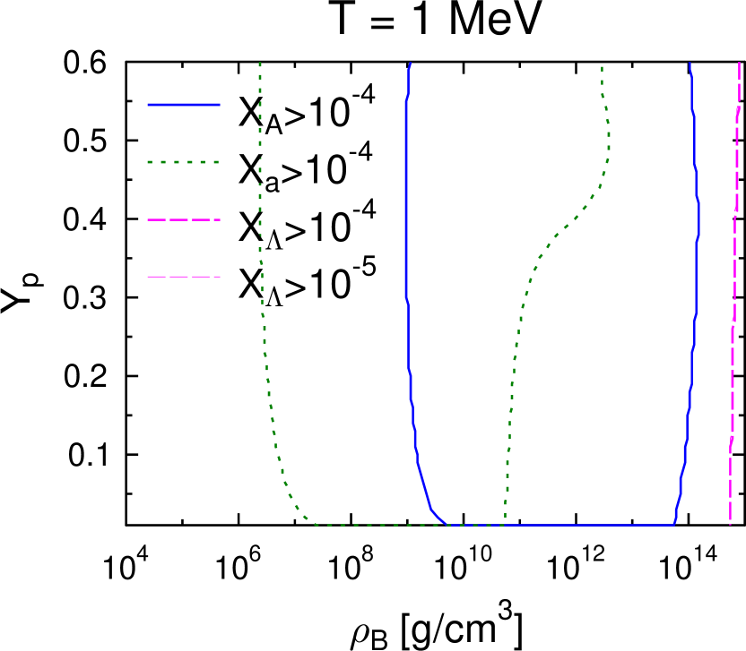
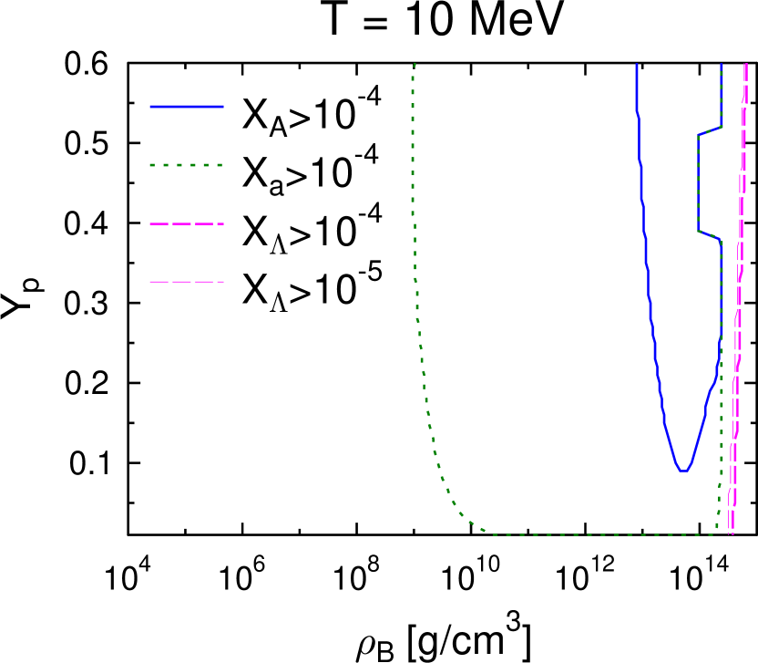
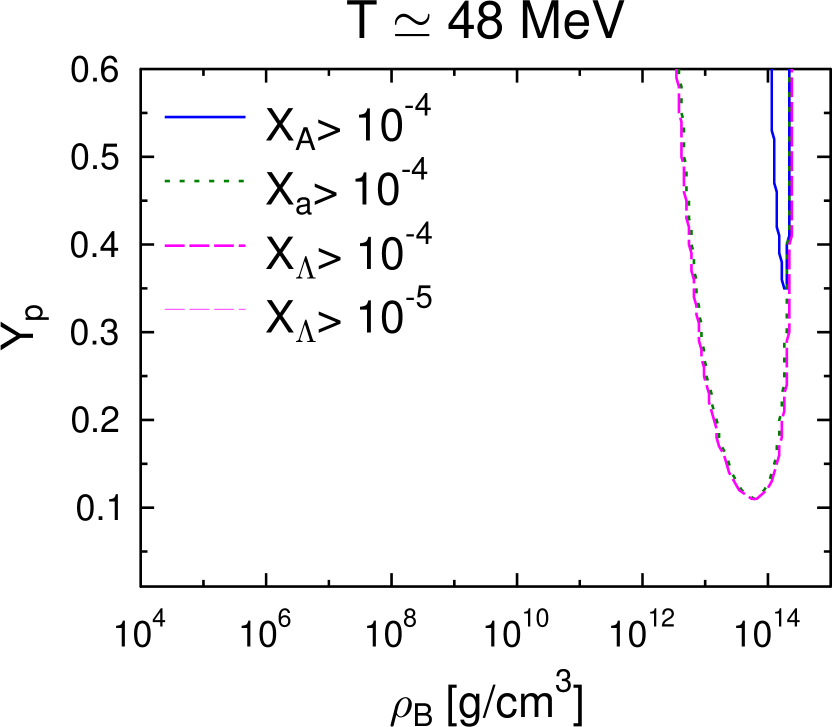
Figure 4: Phase diagram at $T=1$, 10, and $\simeq 48$ MeV (bottom to top) in the $Y_{p}$-$\rho_{B}$ plane for the BHB$\Lambda\phi$ EoS. The lines delimit regions where the mass fractions of light nuclei ($X_{a}$), heavy nuclei ($X_{A}$) and $\Lambda$s ($X_{\Lambda}$) exceed $10^{-4}$. The thin dashed magenta line also shows where the mass fraction of $\Lambda$s exceeds $10^{-5}$. For $T=1$ and 10 MeV, $\Lambda$s occur abundantly only at high densities. For $T\simeq 48$ MeV, the isocontours of light nuclei and $\Lambda$s almost coincide.

Figure 4 gives complementary information about the composition by showing “phase diagrams” in the $Y_{p}$-$\rho_{B}$ space. For $T=10$ MeV, there is an unexpected kink for $X_{A}$ for $Y_{p}$ between 0.4 and 0.5. This is probably related to the limitation of the composition in the HS(DD2) model regarding the maximum asymmetry and mass number that nuclei can have. In the bottom panel of Figure 4, a temperature of $\simeq 48$ MeV is selected. Note again that for $T\geq 50$ MeV, the HS model does not take into account the formation of nuclei. The temperature of $\simeq 48$ MeV corresponds to the highest temperature in our final EoS tables, where nuclei can, in principle, still appear. It is important to note that the small fraction of “heavy” nuclei $X_{A}$ that can be seen in Figure 4 at this high temperature, actually corresponds to intermediate mass nuclei such as carbon. Here the abundance of nuclei is decreasing exponentially with their mass number. At the temperature of $\simeq 48$ MeV we find that the lines for $\Lambda$s almost coincide with those of light nuclei. For moderate asymmetries (e.g., $Y_{p}=0.3$), an isothermal compression would lead to a transition from np$\Lambda$-matter to a mixture of nucleons and light nuclei, and then above $\sim 10^{14}$ g/cm³ back to np$\Lambda$-matter. This “peninsula” of light nuclei must be seen as a result of the minimization of the free energy. For very low densities and such high temperatures, there would be almost no nuclei present. Instead, there is a thermal contribution of $\Lambda$s that makes them the favorite phase. At intermediate densities, light nuclei play a more important role than $\Lambda$s. At high densities, where the formation of $\Lambda$s is driven by density and by high chemical potentials, they again form the most stable phase. As mentioned earlier, a more detailed calculation should, in principle, consider all possible degrees of freedom at all conditions.

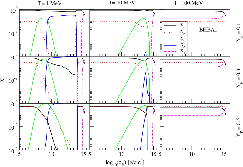
Figure 5: Mass fractions of neutrons ($X_{n}$), protons ($X_{p}$), light nuclei ($X_{a}$), heavy nuclei ($X_{A}$), and $\Lambda$ hyperons ($X_{\Lambda}$) are plotted as a function of baryon mass density for BHB$\Lambda\phi$ corresponding to the np$\Lambda\phi$ case.

Figure 5 exhibits the composition of supernova matter at different regimes of temperatures, proton fractions and densities. Fractions of neutrons ($X_{n}$), protons ($X_{p}$), light nuclei ($X_{a}$), heavy nuclei ($X_{A}$), and $\Lambda$s ($X_{\Lambda}$) are shown as a function of baryon mass density for $T=1$, 10 and 100 MeV and $Y_{p}=$ 0.1, 0.3 and 0.5, for the np$\Lambda\phi$ case. For $T=1$ MeV and $Y_{p}=$ 0.1, almost only free neutrons and protons exist up to a mass density of $\sim 10^{7}$ g/cm³. Beyond this density point, the free proton fraction drops sharply because protons are now bound inside light nuclei coexisting with free neutrons, which at this low temperature are mostly alpha-particles. Similarly, the free neutron fraction is reduced. The shape of the curve for light nuclei tends to be symmetric and the width of it increases with higher values of proton fraction. Heavy nuclei ($Z\geq 6$) start populating the system around $10^{9}$ g/cm³ replacing light nuclei. This trend is noted also for other values of proton fractions. The fraction of heavy nuclei grows and reaches its maximum value at higher mass densities with an increasing proton fraction as is evident from the $T=1$ MeV panel of Figure 5. Consequently, fractions of free neutrons and light nuclei fall rapidly. Heavy nuclei dissolve into their fundamental constituents at $\sim 10^{14}$ g/cm³ and form a uniform matter of neutrons and protons. It is observed that $\Lambda$ hyperons appear with significant abundance at a density above 2$n_{0}$ at the cost of neutrons when the zero-temperature threshold condition $\mu_{\Lambda}=\mu_{n}\geq m_{\Lambda}$ is satisfied. The higher the proton fraction, the smaller the population of $\Lambda$s. Note again that we include $\Lambda$ hyperons in the hyperon EoS tables only when its fraction is above $10^{-5}$.

Now we focus on the case of $T=10$ MeV of Figure 5 (middle panel). Here light nuclei are formed replacing free nucleons at higher mass densities. Though significant populations of light nuclei are noted for different $Y_{p}$, the distribution of heavy nuclei is appreciable and very sharp only for $Y_{p}=$ 0.5. It was found that just like the $T=1$ MeV case, nuclei melt down to form a uniform nuclear matter before the saturation density is reached and $\Lambda$s appear at higher densities. For $T=1$ and 10 MeV, we do not find any thermal $\Lambda$s as expected.

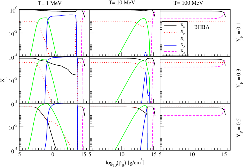
Figure 6: Mass fractions of neutrons ($X_{n}$), protons ($X_{p}$), light nuclei ($X_{a}$), heavy nuclei ($X_{A}$), and $\Lambda$ hyperons ($X_{\Lambda}$) are plotted as a function of baryon mass density for BHB$\Lambda$ corresponding to the np$\Lambda$ case.

Next we discuss the case of $T=100$ MeV in Figure 5 (right panel). Note that in the HS(DD2)-EoS nuclei are only considered up to a temperature of 50 MeV, because their contribution is small for such high temperatures. Thus, only uniform matter of neutrons, protons and $\Lambda$s is found to exist in this case. A significant fraction of $\Lambda$ hyperons is thermally produced at low densities with the constraint $\mu_{n}=\mu_{\Lambda}$ and it grows with density at the expense of neutrons. We find qualitatively similar behavior for the hyperon case without $\phi$ mesons as shown in Figure 6. The only difference between the np$\Lambda$ and np$\Lambda\phi$ cases is found in $\Lambda$ fraction at high densities as is also evident from Tables 4 - 11 which show excerpts from our full EoS tables.

These tables also show that very low values of the effective Dirac masses are found at very high densities. Small or even negative values of the nucleon effective Dirac mass are well known to occur in relativistic mean-field models (see Zimanyi & Moszkowski (1990); Schaffner & Mishustin (1996)). In our case with $T=0.1$ MeV, vanishingly small or negative values of the nucleon effective Dirac mass occur beyond the central density, corresponding to the maximum neutron star mass.

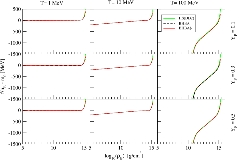
Figure 7: Free energy per baryon with respect to $m_{0}=938$ MeV is plotted as a function of baryon mass density for temperatures $T=$1, 10, 100 MeV and proton fractions $Y_{p}=$ 0.1, 0.3 and 0.5. Results from the nucleonic EoS table HS(DD2) (online-version: green) and the two hyperon EoS tables BHB$\Lambda$ (dashed line) and BHB$\Lambda\phi$ (online-version: red) are shown here.

Free energy per baryon is shown as a function of baryon mass density in Figure 7. Here and in all following plots, we only show the baryonic contribution. Free energy per baryon is measured with respect to the arbitrary value of $m_{0}=938$ MeV. This figure also shows various regimes of temperatures, $T=$ 1, 10 and 100 MeV, and proton fractions, $Y_{p}=$ 0.1, 0.3 and 0.5. Furthermore, the results of hyperon matter with (solid line) and without (dashed line) $\phi$ mesons are shown in Figure 7. At lower densities, there is practically no difference between the results of nuclear and hyperon matter for different situations considered. This may be attributed to no $\Lambda$s for $T=$ 1 and 10 MeV or just a low abundance of thermal $\Lambda$s in the case of $T=$ 100 MeV as shown in the previous figures. On the other hand, the free energy is reduced when $\Lambda$s are populated significantly at higher densities and higher temperatures compared with the nuclear EoS. It is noted that when hyperon-hyperon interaction is mediated by $\phi$ mesons in the np$\Lambda\phi$ case, the free energy is higher than that of the np$\Lambda$ case.

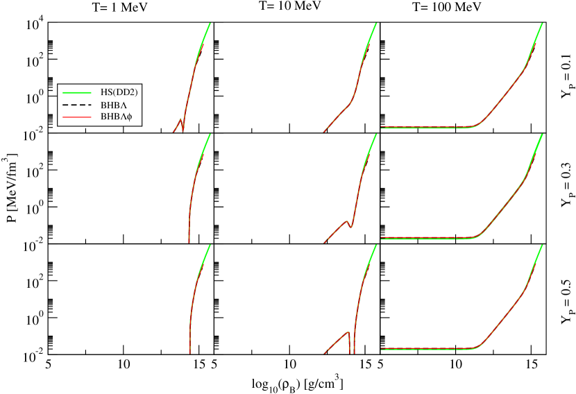
Figure 8: Pressure is exhibited as a function of baryon mass density for temperatures $T=$1, 10, 100 MeV and proton fractions $Y_{p}=$ 0.1, 0.3 and 0.5. Results from the nucleonic EoS table HS(DD2) (online-version: green) and the two hyperon EoS tables BHB$\Lambda$ (dashed line) and BHB$\Lambda\phi$ (online-version: red) are shown here.

Pressure as a function baryon mass density is displayed in Figure 8 for temperatures $T=$ 1, 10 and 100 MeV and proton fractions $Y_{p}=$ 0.1, 0.3 and 0.5. Just like the free energy case, we find the hyperon EoS with and without $\phi$ mesons at high densities and temperatures to be softer than the nuclear EoS. Furthermore, the hyperon EoS in the np$\Lambda\phi$ case is stiffer than the hyperon EoS in the np$\Lambda$ case. It is worth noting here that there is no kink or jump in pressure when $\Lambda$s appear in the system. This indicates that it is a smooth transition from nuclear to hyperon matter.

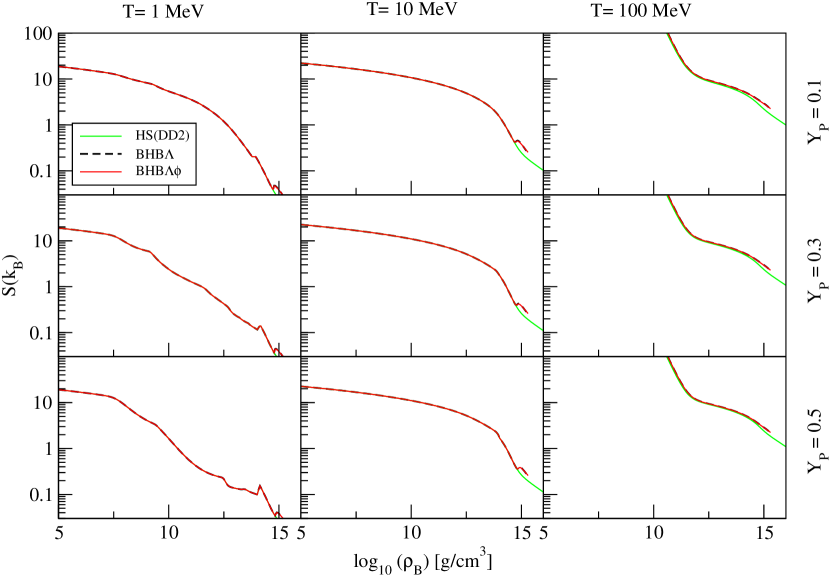
Figure 9: Entropy per baryon is shown as a function of baryon mass density for temperatures $T=$1, 10, 100 MeV and proton fractions $Y_{p}=$ 0.1, 0.3 and 0.5. Results from the nucleonic EoS table HS(DD2) (online-version: green) and the two hyperon EoS tables BHB$\Lambda$ (dashed line) and BHB$\Lambda\phi$ (online-version: red) are shown here.

Figure 9 demonstrates the behavior of entropy per baryon as a function of baryon mass density. We consider the same values of temperatures and proton fractions as before. For low temperatures, there is not much difference between the results with or without $\Lambda$ hyperons. Note that the kinks at low densities originate from changes in the nuclear composition which are related to nuclear shell effects. There are some effects of $\Lambda$ hyperons for higher baryon densities at $T=$ 10 MeV . As the temperature increases to $T=$ 100 MeV, this difference is pronounced. In this case, the entropy per baryon including $\Lambda$ hyperons is higher than that of the nuclear matter. However, we cannot differentiate between the results of hyperon matter with and without $\phi$ mesons.

Examples of data from hyperon EoS tables with and without $\phi$ mesons are recorded in Tables 4 - 11. For $T=$ 0.1, 10 and 100 MeV, selected rows of the main tables with fixed values of $Y_{p}$ and baryon mass density ($\rho_{B}$) are displayed in those tables. The various quantities are explained in Appendix A.2. Two variants of the hyperon EoS tables with (BHB$\Lambda\phi$) and without (BHB$\Lambda$) $\phi$ mesons in binary as well as Shen98 formats are available online. Both hyperon EoS tables are also available in the comprehensive CompOSE EoS database as well as on the stellarcollapse.org Web site. Tables in Shen98 format do not include electrons, positrons, and photons whereas binary data files of EoS tables take into account the contributions of electrons, positrons and photons. Further details are given on the Web site of footnote 1.

4 Summary and Conclusions

We have constructed hyperon EoS tables including $\Lambda$ hyperons for supernova simulations and neutron stars in a density dependent relativistic mean field model. We also take into account the $\Lambda$-$\Lambda$ interaction mediated by $\phi$ mesons in this calculation. The nuclear statistical equilibrium model of Hempel & Schaffner-Bielich (2010) is adopted for the description of matter made of light and heavy nuclei coexisting with unbound nucleons below saturation densities and temperatures up to 50 MeV. We have denoted the calculation including $\Lambda$ hyperons without $\phi$ mesons as the np$\Lambda$ case and that of the $\Lambda$ hyperons with $\phi$ mesons as the np$\Lambda\phi$ case. The DD2 parameter set Typel et al. (2010) has been used in this calculation for the nucleons. The vector meson - $\Lambda$ hyperon couplings are obtained from the SU(6) symmetry relations of the quark model, whereas the scalar meson - $\Lambda$ hyperon coupling is determined from the potential depth of the $\Lambda$ hyperon in nuclear matter at the saturation density of $-30$ MeV which is extracted from the experimental binding energies of $\Lambda$ hypernuclei. The system is populated with $\Lambda$s using the equilibrium condition $\mu_{n}=\mu_{\Lambda}$. The contribution of $\Lambda$s is considered in our calculation when its corresponding EoS gives a lower free energy than the EoS of only nuclei and nucleons and when the $\Lambda$ mass fraction exceeds $10^{-5}$ at the same time. It is noted that the fraction of $\Lambda$ hyperons is negligible at low-density and low-temperature domains. The population of $\Lambda$ hyperons grows in uniform matter at the cost of neutrons at high density. A significant fraction of thermal $\Lambda$ hyperons is populated in the system at higher temperatures.

The free energy of the system including $\Lambda$ hyperons is lower compared to that of the nuclear matter case. However, $\Lambda$ hyperon matter involving $\phi$ mesons has higher free energy than that of the $\Lambda$ hyperon matter without $\phi$ mesons. Regarding the entropy per baryon, one notices that it is higher than in the case of nuclear matter when more degrees of freedom in the form of $\Lambda$ hyperons appear in the system. This indicates different thermal properties of the EoS, which are known to be important for neutron-star mergers (Bauswein et al., 2013; Kaplan et al., 2013) and black hole formation (Hempel et al., 2012). We observe that the EoS (pressure versus baryon mass density) of the $\Lambda$ hyperon matter with and without $\phi$ mesons is softer than the nuclear EoS. Furthermore, the repulsive interaction of $\phi$ mesons makes the EoS of the np$\Lambda\phi$ case stiffer than that of the np$\Lambda$ case. It is important to note that the pressure grows smoothly with baryon density even after the appearance of $\Lambda$ hyperons. We did not find any indication for a first-order phase transition connected with the appearance of hyperons, as discussed, e.g., by Schaffner-Bielich et al. (2002); Gulminelli (2012, 2013).

We have generated two $\Lambda$ hyperon EoS tables with (BHB$\Lambda\phi$) and without (BHB$\Lambda$) $\phi$ mesons covering temperatures (0.1 – 158.48 MeV), proton fractions (0.01 – 0.6), and baryon density ($10^{-12}$ – $\simeq$1 fm^-3). The EoS tables are written in two different formats: the first format is similar to the one used by Shen et al. (1998), and the second one corresponds to extended tables including electrons, positrons and photons in a binary format. Tables 4 - 11 illustrate certain parts of the main tables.

Finally, we impose the charge neutrality and $\beta$-equilibrium in our $\Lambda$ hyperon EoS tables and calculate mass-radius relationship of the neutron star sequence at $T=0.1$ MeV. We obtain maximum neutron star masses 2.1 M_⊙ and 1.95 M_⊙ corresponding to the $\Lambda$ hyperon EoS with and without $\phi$ mesons, respectively. The maximum neutron star mass of $\Lambda$ hyperon matter including $\phi$ mesons is compatible with the recently measured 2.01$\pm$0.04 M_⊙ neutron star.

We shall perform supernova simulations with new hyperon EoS tables and publish those results separately in the future. New hyperon EoS tables will be also useful for neutron star merger calculations.

Appendix

Appendix A Description of the Tables in Shen98 Format

The EoS tables are presented in two different formats “Extended” and “Shen98” on the Web site http://phys-merger.physik.unibas.ch/~hempel/eos.html Here we restrict ourselves to the description of the latter where the information are stored in a format that is similar to the tables of Shen (Shen et al., 1998, 2011c), which is widely used in many different astrophysical applications.

A.1 Parameter Grid and Data Structure

Table 3 gives an overview of the two hyperonic tables BHB$\Lambda$ and BHB$\Lambda\phi$, regarding the constituents considered, and the points in the parameter space of temperature, density, and proton fraction which were calculated. For density and temperature, we have a logarithmic spacing, and for the proton fraction it is linear. Besides the range of density, the two tables cover the same conditions (i.e., in temperature and proton fraction).

We arrange the data as follows: We group them in blocks of constant temperature, starting with the lowest value. Within each temperature block, we group the data according to the proton fraction, again starting with lowest values. For given temperature and proton fraction, we list all baryon number densities with increasing values.

A.2 Entries of the Tables

For each grid point specified by density, temperature, and electron fraction, there are 20 different thermodynamic quantities in the tables. Those thermodynamic quantities are explained below. Note that only baryonic contributions to different quantities are recorded. The contributions of photons, electrons, positrons, and neutrinos are to be added separately.

1. Logarithm of baryon mass density (log${}_{10}(\rho_{B})$ [g/cm³]).

   The baryon mass density is defined as the baryon number density multiplied by the value of the atomic mass unit $m_{u}=$ 931.49432 MeV.

2. Baryon number density ($n_{B}$ [fm^-3]).

3. Logarithm of total proton fraction (log${}_{10}(Y_{p})$ []) .

4. Total proton fraction ($Y_{p}$ []).

   Note that the total proton fraction $Y_{p}$ is given by all protons (i.e., free and bound in nuclei) and thus is equal to the electron fraction to obtain charge neutrality.

5. Free energy per baryon ($F$ [MeV]).

   Free energy per baryon relative to 938 MeV is defined by

   $$F=\frac{f}{n_{B}}-938~{}.$$ (A1)

   We have chosen the reference value of 938 MeV because it was also used in the original table of Shen et al. (1998). Note that this value is otherwise completely arbitrary and not used in the EoS calculations.

6. Internal energy per baryon ($E_{\rm int}$ [MeV]).

   $E_{\rm int}$ relative to $m_{u}$ is defined by

   $$E_{\rm int}=\frac{\epsilon}{n_{B}}-m_{u}~{}.$$ (A2)

7. Entropy per baryon ($S$ [$k_{B}$]).

8. Average mass number of heavy nuclei ($\bar{A}$ []).

   This is defined as $\bar{A}=\sum_{A,Z\geq 6}An_{A,Z}/\sum_{A,Z\geq 6}n_{A,Z}$.

9. Average charge number of heavy nuclei ($\bar{Z}$ []).

   This is defined as $\bar{Z}=\sum_{A,Z\geq 6}Zn_{A,Z}/\sum_{A,Z\geq 6}n_{A,Z}$.

   Note that $\bar{Z}$ and $\bar{A}$ are set to zero if $X_{A}=0$, i.e., if no heavy nuclei are present.

10. Nucleon effective Dirac mass ($m^{*}$ [MeV]).

    In the RMF calculation, we use separate values for neutron and proton masses. However, we store only the average value of neutron and proton effective Dirac masses.

11. Mass fraction of unbound neutrons ($X_{n}$ []).

    This is defined as $X_{n}=n_{n}/n_{B}$.

12. Mass fraction of unbound protons ($X_{p}$ []).

    It is given by $X_{p}=n_{p}/n_{B}$.

13. Mass fraction of light nuclei ($X_{a}$ []).

    This is defined as $X_{a}=\sum_{A,Z\leq 5}An_{A,Z}/n_{B}$.

14. Mass fraction of heavy nuclei ($X_{A}$ []).

    This is defined as $X_{A}=\sum_{A,Z\geq 6}An_{A,Z}/n_{B}$.

15. Baryon pressure ($P$ [MeV/fm³]).

16. Neutron chemical potential relative to neutron rest mass ($\mu_{n}-m_{n}$ [MeV]).

    The value of $m_{n}$ is specified in Table LABEL:table2, which also corresponds to the value used in our calculations. Note that $\mu_{\Lambda}=\mu_{n}$ wherever $\Lambda$s are present.

17. Proton chemical potential relative to proton rest mass ($\mu_{p}-m_{p}$ [MeV]).

    The value of $m_{p}$ is specified in Table LABEL:table2, which also corresponds to the value used in our calculations.

18. Average mass number of light nuclei ($\bar{a}$ []).

    This is defined as $\bar{a}=\sum_{A,Z\leq 5}An_{A,Z}/\sum_{A,Z\leq 5}n_{A,Z}$.

19. Average charge number of light nuclei ($\bar{z}$ []).

    This is defined as $\bar{z}=\sum_{A,Z\leq 5}Zn_{A,Z}/\sum_{A,Z\leq 5}n_{A,Z}$.

    Note that $\bar{z}$ and $\bar{a}$ are set to zero if $X_{a}=0$, i.e., if no light nuclei are present.

20. Mass fraction of Lambda hyperons ($X_{\Lambda}$ []).

    It is defined as $X_{\Lambda}=n_{\Lambda}/n_{B}$.

A.3 Accuracy and Consistency of the EoS Tables

We have performed the following consistency checks on the EoS tables.

1. Thermodynamic consistency requires

   $$\epsilon=Ts-P+\mu_{n}(1-Y_{p})n_{B}+\mu_{p}Y_{p}n_{B}~{}.$$ (A3)

   The modulus of the relative thermodynamic accuracy

   $$\Delta=\frac{Ts-P+\mu_{n}(1-Y_{p})n_{B}+\mu_{p}Y_{p}n_{B}}{\epsilon}-1~{},$$ (A4)

   is on average $2.0\times 10^{-6}$ in the EoS tables.

2. Sum rule of particle fractions is given by

   $$X_{n}+X_{p}+X_{a}+X_{A}+X_{\Lambda}=1~{},$$ (A5)

   and is satisfied by the EoS tables with an accuracy higher than $1.8\times 10^{-7}$. The average deviation is $2.6\times 10^{-8}$.

3. We have also checked that the EoS tables fulfill the thermodynamic stability criteria

   $$\frac{\partial{s}}{\partial T}\geq 0~{},$$ (A6)

   and

   $$\frac{\partial P^{\rm tot}}{\partial n_{B}}\geq 0~{}.$$ (A7)

   The second of the two relations is only fulfilled for the total pressure, i.e., if the electron contribution is added $P^{\rm tot}=P_{e}+P$. There are just ten grid points in the table, where this second relation is slightly violated.

Note that all numbers which we have given here are directly calculated from the tables in the Shen98 format. Because only seven digits are stored in these tables, the highest deviations originate mostly from round-off errors. In our actual calculations, and in some other binary versions of the tables where all quantities are stored with double precision, the accuracy is even higher. Note that we also do not apply any smoothing or averaging prescription, as is done in, e.g., Shen et al. (2011a, b).

Table 1: Parameters of Nucleon-Meson Couplings as Defined in Equation (11) and Equation (12)

i	$g_{iN}(n_{0})$	$a_{i}$	$b_{i}$	$c_{i}$	$d_{i}$
$\sigma$	10.686681	1.357630	0.634442	1.005358	0.575810
$\omega$	13.342362	1.369718	0.496475	0.817753	0.638452
$\rho$	3.626940	0.518903

Note. — The parameters are obtained by reproducing properties of finite nuclei and the parameter set is known as the DD2 set (Typel et al., 2010). This parameterization leads to nuclear saturation properties such as saturation density ($n_{0}=0.149065$ fm^-3), binding energy (16.02 MeV), incompressibility of matter (242.7 MeV), symmetry energy (31.67 MeV), and its slope (55.03 MeV). All parameters are dimensionless.

Table 2: Masses of Baryons and Mesons in Units of MeV Used in This Calculation

Neutron	Proton	$\Lambda$	$\sigma$	$\omega$	$\rho$	$\phi$
939.56536	938.27203	1115.7	546.212459	783.0	763.0	1020.0

Table 3: Overview of the EoS Tables Presented in This Paper.

		BHB$\Lambda$	BHB$\Lambda\phi$
Constituents	Uniform matter	$n$, $p$, $\Lambda$	$n$, $p$, $\Lambda$
	Non-uniform matter	$n$, $p$, $\{A,Z\}$	$n$, $p$, $\{A,Z\}$
$T$	Range	$-1.0\leq\log_{10}(T)\leq 2.2$	$-1.0\leq\log_{10}(T)\leq 2.2$
(MeV)	Grid spacing	$\Delta\log_{10}(T)=0.04$	$\Delta\log_{10}(T)=0.04$
	Points	81	81
$Y_{p}$	Range	$0.01\leq Y_{p}\leq 0.60$	$0.01\leq Y_{p}\leq 0.60$
()	Grid spacing	$\Delta Y_{p}=0.01$	$\Delta Y_{p}=0.01$
	Points	60	60
$n_{B}$	Range	$-12\leq\log_{10}(n_{B})\leq 0$	$-12\leq\log_{10}(n_{B})\leq 0.08$
$\rm{(fm^{-3})}$	Grid spacing	$\Delta\log_{10}(n_{B})=0.04$	$\Delta\log_{10}(n_{B})=0.04$
	Points	301	303

Note. — In both tables, non-uniform matter is modeled as a mixture of free neutrons ($n$), free protons ($p$), and an ensemble of heavy nuclei ($\{A,Z\}$). Uniform matter consists in general of neutrons, protons, and $\Lambda$s ($\Lambda$), whereas $\Lambda$s are only considered, when the conditions described in Section 2.3 are met. Besides the range of density, the two tables cover the same conditions (i.e., in temperature and proton fraction).

Table 4: Data from BHB$\Lambda$ EoS Table for $T=0.1$ MeV and $Y_{p}=$ 0.01 and 0.5

$\log_{10}(\rho_{B})$	$n_{B}$	$\log_{10}(Y_{p})$	$Y_{p}$	$F$	$E_{\rm{int}}$	$S$	$\bar{A}$	$\bar{Z}$	$m^{*}$
($\rm{g\,cm^{-3}}$)	($\rm{fm^{-3}}$)			(MeV)	(MeV)	($k_{B}$)			(MeV)
3.22025	1.0E-12	-2	0.01	-0.385878	7.97106	18.5126	76	26	939.565
14.2203	0.1	-2	0.01	11.5293	18.0360	0.010149	0	0	631.434
15.2203	1.0	-2	0.01	288.255	294.761	0.260104E-02	0	0	9.95451
3.22025	1.0E-12	-0.30103	0.5	-7.77206	-1.2157	0.506831	56	28	938.272
14.2203	0.1	-0.30103	0.5	-13.6378	-7.13086	1.29635	0	0	625.119
15.2203	1.0	-0.30103	0.5	305.76	312.266	0.283803E-02	0	0	52.0946

Note. — This table gives the values of quantities of six single rows in the so-called Shen-98-format, as specified in Appendix A.2. The complete hyperon table without $\phi$ mesons (BHB$\Lambda$) is available at http://phys-merger.physik.unibas.ch/~hempel/eos/v1.0/bhb_l_frdm_shen98format.zip. Data points with less digits are shown here for guidance regarding its form and content.

Table 5: Continuation of Table 4

$X_{n}$	$X_{p}$	$X_{a}$	$X_{A}$	$P$	$\mu_{n}$	$\mu_{p}$	$\bar{a}$	$\bar{z}$	$X_{\Lambda}$
				($\rm{MeV\,fm^{-3}}$)	(MeV)	(MeV)
0.970769	0	0	0.02923	0.971141E-13	-1.65569	-20.2045	3.01	1.01	0
0.99	0.01	0	0	0.949866	20.5277	-84.6839	0	0	0
0.248928	0.01	0	0	336.830	626.015	377.824	0	0	0.741072
0	0	0	1	0.153089E-14	-13.739	-3.63947	4	2	0
0.5	0.5	0	0	-0.609824	-20.6929	-20.6166	0	0	0.0
0.088970	0.5	0	0	491.997	693.182	900.493	0	0	0.411030

Table 6: Same as Table 4, but for $T=100$ MeV

$\log_{10}(\rho_{B})$	$n_{B}$	$\log_{10}(Y_{p})$	$Y_{p}$	$F$	$E_{\rm{int}}$	$S$	$\bar{A}$	$\bar{Z}$	$m^{*}$
($\rm{g\,cm^{-3}}$)	($\rm{fm^{-3}}$)			(MeV)	(MeV)	($k_{B}$)			(MeV)
3.22025	1.0E-12	-2	0.01	-2.13589E+10	2.40721E+11	2.62080E+09	0	0	773.734
14.2203	0.1	-2	0.01	-279.137	206.844	4.79475	0	0	542.722
15.2203	1.0	-2	0.01	165.051	411.954	2.40397	0	0	19.9808
3.22025	1.0E-12	-0.30103	0.5	-2.13589E+10	2.40721E+11	2.62080E+09	0	0	854.728
14.2203	0.1	-0.30103	0.5	-341.599	170.628	5.05722	0	0	619.924 5
15.2203	1.0	-0.30103	0.5	177.458	423.538	2.39574	0	0	71.3397

Note. — The complete hyperon table without $\phi$ mesons (BHB$\Lambda$) is available at http://phys-merger.physik.unibas.ch/~hempel/eos/v1.0/bhb_l_frdm_shen98format.zip. Data points with less digits are shown here for guidance regarding its form and content.

Table 7: Continuation of Table 6.

$X_{n}$	$X_{p}$	$X_{a}$	$X_{A}$	$P$	$\mu_{n}$	$\mu_{p}$	$\bar{a}$	$\bar{z}$	$X_{\Lambda}$
				($\rm{MeV\,fm^{-3}}$)	(MeV)	(MeV)
0.814211	0.01	0	0	0.0213589	-939.565	-938.272	0	0	0.175788
0.772041	0.01	0	0	11.4656	-161.377	-627.033	0	0	0.217959
0.274440	0.01	0	0	407.159	573.612	278.197	0	0	0.715560
0.411164	0.5	0	0	0.0213589	-939.565	-938.272	0	0	0.0888365
0.408025	0.5	0	0	11.2739	-242.685	-216.873	0	0	0.091975
0.105272	0.5	0	0	554.206	614.827	846.663	0	0	0.394728

Table 8: Same as Table 4, but now for the BHB$\Lambda\phi$ EoS table for T = 10 MeV.

$\log_{10}(\rho_{B})$	$n_{B}$	$\log_{10}(Y_{p})$	$Y_{p}$	$F$	$E_{\rm{int}}$	$S$	$\bar{A}$	$\bar{Z}$	$m^{*}$
($\rm{g\,cm^{-3}}$)	($\rm{fm^{-3}}$)			(MeV)	(MeV)	($k_{B}$)			(MeV)
3.22025	1.0E-12	-2	0.01	-243.554	23.2555	26.0303	8	6	939.552
14.2203	0.1	-2	0.01	7.01729	22.2363	0.871332	19.81	6	633.164
15.2203	1	-2	0.01	331.522	340.708	0.268107	0	0	29.9543
3.22025	1.0E-12	-0.30103	0.5	-250.549	22.6219	26.6665	8	6	938.919
14.2203	0.1	-0.30103	0.5	-19.8927	-1.34810	1.20389	0	0	627.659
15.2203	1.0	-0.30103	0.5	319.375	328.752	0.287131	0	0	61.3811

Note. — The complete hyperon table with $\phi$ mesons (BHB$\Lambda\phi$) is available at http://phys-merger.physik.unibas.ch/~hempel/eos/v1.0/bhb_lp_frdm_shen98format.zip. Data points with less digits are shown here for guidance regarding its form and content.

Table 9: Continuation of Table 8.

$X_{n}$	$X_{p}$	$X_{a}$	$X_{A}$	$P$	$\mu_{n}$	$\mu_{p}$	$\bar{a}$	$\bar{z}$	$X_{\Lambda}$
				($\rm{MeV\,fm^{-3}}$)	(MeV)	(MeV)
0.99	0.01	0	0	1.0E-11	-234.647	-280.577	2	1	0
0.989845	0.009922	0.000232	0	1.32322	19.9713	-107.445	3.11	1.04	0
0.414247	0.01	0	0	448.471	781.568	468.839	0	0	0.575753
0.5	0.5	0	0	1.0E-11	-241.478	-241.457	2	1	0
0.5	0.5	0	0	-0.069936	-21.5511	-21.4705	0	0	0.0
0.149693	0.5	0	0	533.660	773.293	930.939	0	0	0.350307

Table 10: Same as Table 8, but for $T=100$ MeV.

$\log_{10}(\rho_{B})$	$n_{B}$	$\log_{10}(Y_{p})$	$Y_{p}$	$F$	$E_{\rm{int}}$	$S$	$\bar{A}$	$\bar{Z}$	$m^{*}$
($\rm{g\,cm^{-3}}$)	($\rm{fm^{-3}}$)			(MeV)	(MeV)	($k_{B}$)			(MeV)
3.22025	1.0E-12	-2	0.01	-2.13590E+10	2.40721E+11	2.62080E+09	0	0	773.746
14.2203	0.1	-2	0.01	-278.401	205.785	4.77680	0	0	549.326
15.2203	1.0	-2	0.01	208.007	455.691	2.41179	0	0	39.9208
3.22025	1.0E-12	-0.30103	0.5	-2.13590E+10	2.40721E+11	2.62080E+09	0	0	854.734
14.2203	0.1	-0.30103	0.5	-341.465	170.346	5.05305	0	0	621.205
15.2203	1.0	-0.30103	0.5	191.740	438.178	2.39932	0	0	79.6312

Note. — The complete hyperon table with $\phi$ mesons (BHB$\Lambda\phi$) is available at http://phys-merger.physik.unibas.ch/~hempel/eos/v1.0/bhb_lp_frdm_shen98format.zip. Data points with less digits are shown here for guidance regarding its form and content.

Table 11: Continuation of Table 10.

$X_{n}$	$X_{p}$	$X_{a}$	$X_{A}$	$P$	$\mu_{n}$	$\mu_{p}$	$\bar{a}$	$\bar{z}$	$X_{\Lambda}$
				($\rm{MeV\,fm^{-3}}$)	(MeV)	(MeV)
0.814225	0.01	0	0	0.0213589	-939.565	-938.272	0	0	0.175775
0.782574	0.01	0	0	11.5394	-159.885	-627.353	0	0	0.207427
0.414758	0.01	0	0	504.552	714.667	348.584	0	0	0.575242
0.411170	0.5	0	0	0.0213589	-939.565	-938.272	0	0	0.0888298
0.410135	0.5	0	0	11.2864	-242.108	-216.932	0	0	0.089865
0.153005	0.5	0	0	588.225	687.012	871.080	0	0	0.346994

References

- Antoniadis et al. (2013) Antoniadis, J., Freire, P. C. C., Wex, N., et al. 2013, Science, 340, 448
- Aparicio (1998) Aparicio, J. M. 1998, Astrophys. J. Suppl. Ser. 117, 627
- Audi et al. (2003) Audi, G., Wapstra, A. H., & Thibault, C. 2003, Nucl. Phys. A, 729, 337
- Banik (2014) Banik, S. 2014, Phys. Rev. C, 89, 035807
- Banik & Bandyopadhyay (2002) Banik, S., & Bandyopadhyay, D. 2002, Phys. Rev. C, 66, 065801
- Bauswein et al. (2013) Bauswein, A., Goriely, S., & Janka, H.-T. 2013, Astrophys. J., 773, 78
- Bethe (1990) Bethe, H. A. 1990, Rev. Mod. Phys., 62, 801
- Bethe & Wilson (1985) Bethe, H. A., & Wilson, J. R. 1985, Astrophys. J., 295, 14
- Blinnikov et al. (2011) Blinnikov, S. I., Panov, I. V., Rudzsky, M. A., & Sumiyoshi, K. 2011, Astron. Astrophys. 535, A37
- Botvina & Mishustin (2004) Botvina, A. S., & Mishustin, I. N. 2004, Phys. L. B 584, 233
- Botvina & Mishustin (2010) Botvina, A. S., & Mishustin, I. N. 2010, Nucl. Phys. A 843, 98
- Brat et al. (1999) Brat, S., Chrien, R. E., Franklin, W. A., et al. 1999, Phys. Rev. Lett., 83, 5238
- Burrows & Lattimer (1984) Burrows, A., & Lattimer, J. M. 1984, Astrophys. J., 285, 294
- Buyukcizmeci et al. (2013b) Buyukcizmeci, N., Botvina, A. S., & Mishustin, I. N. 2014, Astrophys. J., 789, 33
- Buyukcizmeci et al. (2013a) Buyukcizmeci, N., Botvina, A. S., Mishustin, I. N., et al. 2013, Nucl. Phys. A, 907, 13.
- Colucci & Sedrakian (2013) Colucci, G., & Sedrakian, A. 2013, Phys. Rev. C, 87, 055806
- Constantinou et al. (2014) Constantinou, C., Muccioli, B., Prakash, M., & Lattimer, J. M. 2014, Phys. Rev. C, 89, 065802
- Dover & Gal (1985) Dover, C. B., & Gal, A. 1985, Prog. Part. Nucl. Phys., 12, 171
- Fái & Randrup (1982) Fái, G., & Randrup, J. 1982 Nucl. Phys. A, 381, 557
- Fischer et al. (2014) Fischer, T., Hempel, M., Sagert, I., Suwa, Y., & Schaffner-Bielich, J. 2014, Eur. Phys. J. A, 50, 46
- Fischer et al. (2011) Fischer, T., Sagert, I., Pagliara, G., et al. 2011, Astrophys. J. Suppl. Ser., 194, 39
- Gal & Millener (2011) Gal, A., & Millener, D. 2011, Phys. Lett. B, 701, 342
- Glendenning (1985) Glendenning, N. K. 1985, Astrophys. J. 293, 470.
- Glendenning (2000) Glendenning, N. K. 2000, Compact Stars (New York: Springer)
- Gong et al. (2001) Gong, Z., Zejda, L., Däppen, W., & Aparicio, J. M. 2001, Computer Physics Communications 136, 294
- Gulminelli (2012) Gulminelli, F., Raduta, Ad. R., & Oertel, M. 2012, Phys. Rev. C, 86, 025805
- Gulminelli (2013) Gulminelli, F., Raduta, Ad. R., Oertel, M., & Margueron, J. 2013, Phys. Rev. C, 87, 055809
- Gusakov et al. (2014) Gusakov, M. E., Haensel, P., & Kantor E. M. 2014, Mon. Not. R. Astron. Soc., 439, 318
- Hempel et al. (2012) Hempel, M., Fischer, T., Schaffner-Bielich, J., & Liebendörfer, L. 2012, Astrophys. J., 748, 70
- Hempel & Schaffner-Bielich (2010) Hempel, M., & Schaffner-Bielich, J. 2010, Nucl. Phys. A, 837, 210
- Hempel et al. (2011) Hempel, M., Schaffner-Bielich, J., Typel, S., & Röpke, G. 2011, Phys. Rev. C, 84, 055804
- Hofmann et al. (2001a) Hofmann, F., Keil, C. M., & Lenske, H. 2001a, Phys. Rev. C, 64, 034314
- Hofmann et al. (2001b) Hofmann, F., Keil, C. M., & Lenske, H. 2001b, Phys. Rev. C, 64, 025804
- Ishizuka et al. (2008) Ishizuka, C., Ohnishi, A., Tsubakihara, K., Sumiyoshi, K., & Yamada, S. 2008, J. Phys. G, 35, 085201
- Janka (2012) Janka, H.-T. 2012, Annu. Rev. Nucl. Part. Sci., 62, 407
- Juodagalvis et al. (2010) Juodagalvis, A., Langanke, K., Hix, W. R., Martinez-Pinedo, G. & Sampaio, J. M. 2010, Nucl. Phys. A, 848, 454
- Kaplan et al. (2013) Kaplan, J. D., Ott, C. D., O’Connor, E. P., et al. 2014, Astrophys. J., 790, 19
- Lastowiecki et al. (2012) Lastowiecki, R., Blaschke, H., Grigorian, H., & Typel, S. 2012, Acta Phys. Polon. Suppl., 5, 535
- Lattimer & Lim (2013) Lattimer, J. M., & Lim, Y. 2013, Astrophys. J., 771, 51
- Lattimer & Swesty (1991) Lattimer, J. M., & Swesty, F. D. 1991, Nucl. Phys. A, 535, 331
- Lopes & Menezes (2013) Lopes, L. L., & Menezes, D. P. 2014, Phys. Rev. C, 89, 02805
- Mares et al. (1995) Mares, J., Friedman, E., Gal, A., & Jennings, B. 1995, Nucl. Phys. A, 594, 311
- Millener et al. (1988) Millener, D. J., Dover, C. B., & Gal, A. 1988, Phys. Rev. C, 38, 2700
- Möller et al. (1995) Möller, P., Nix, J. R., Myers, W. D., & Swiatecki, W. J. 1995, Atomic Data and Nuclear Data Tables, 59, 185
- Nakazawa et al. (2010) Nakazawa, K. KEK-E176 collaborators, E373 collaborators, & J-PARC E07 collaborators, 2010, Nucl. Phys. A, 835, 207
- Nakazato et al. (2012) Nakazato, K., Furusawa, S., Sumiyoshi, K., et al. 2012 Astrophys. J., 745, 197
- Nakazato et al. (2008) Nakazato, K., Sumiyoshi, K., & Yamada, S. 2008, Phys. Rev. D, 77, 103006
- Nordhaus et al. (2010) Nordhaus, J., Burrows, A., Almgren, A., & Bell, J. 2010, Astrophys. J., 720, 694
- Oertel et al. (2012) Oertel, M., Fantina, A. F., & Novak, J. 2012, Phys. Rev. C, 85, 055806
- Pagliara et al. (2014) Pagliara, G., Drago, A., Lavagno, A., & Pigato, D. 2014, Acta Phys. Polon. Supp., 7, 451
- Peres et al. (2013) Peres, B., Oertel, M., & Novak, J. 2013, Phys. Rev. D, 87, 043006
- Providência (2013) Providência, C., & Rabhi, A., 2013, Phys. Rev. C 87, 055801
- Qin et al. (2012) Qin, L., Hagel, K., Wada, R., et al. 2012, Phys. Rev. Lett., 108, 172701
- Raduta & Gulminelli (2010) Raduta, Ad. R., & Gulminelli, F. 2010, Phys. Rev. C, 82, 065801
- Sagert et al. (2009) Sagert, I., Fischer, T., Hempel, M., Pagliara, G., & Schaffner-Bielich, J. 2009, Phys. Rev. Lett., 102, 081101
- Schaffner & Gal (2000) Schaffner, J., & Gal, A. 2000, Phys. Rev. C, 62, 034311
- Schaffner & Mishustin (1996) Schaffner, J., & Mishustin, I. N. 1996, Phys. Rev. C, 53, 1416
- Schaffner et al. (1992) Schaffner, J., Stöcker, H., & Greiner, C. 1992, Phys. Rev. C, 46, 322
- Schaffner-Bielich et al. (2002) Schaffner-Bielich, J., Hanauske, M., Stöcker, H., & Greiner, W. 2002, Phys. Rev. Lett., 89, 171101
- Shen et al. (2011b) Shen, G., Horowitz, C. J., & O’Connor, E. 2011a, Phys. Rev. C, 83, 065808
- Shen et al. (2010) Shen, G., Horowitz, C. J., & Teige, S. 2010, Phys. Rev. C, 82, 045802
- Shen et al. (2011a) Shen, G., Horowitz, C. J., & Teige, S. 2011b, Phys. Rev. C, 83, 035802
- Shen et al. (1998) Shen, H., Toki, H., Oyamatsu, K., & Sumiyoshi, K. 1998, Nucl. Phys. A, 637, 435
- Shen et al. (2011c) Shen, H., Toki, H., Oyamatsu, K., & Sumiyoshi, K. 2011c, Astrophys. J. Suppl. Ser., 197, 20
- Steiner et al. (2013) Steiner, A., Hempel, M., & Fischer, T. 2013, Astrophys. J., 774, 17
- Sumiyoshi et al. (2009) Sumiyoshi, K., Ishizuka, C., Ohnishi, A., Yamada, S., & Suzuki, H. 2009, Astrophys. J., 690, L43
- Sumiyoshi & Röpke (2008) Sumiyoshi, K., & Röpke, G. 2008, Phys. Rev. C, 77, 055804
- Takahashi et al. (2001) Takahashi H., Ahn J. K., Akikawa H., et al. 2001, Phys. Rev. Lett., 87, 212502
- Togashi et al. (2014) Togashi, H., Takano, H., Sumiyoshi, K., & Nakazato, K. 2014, Prog. Theor. Exp. Phys., 023D05
- Typel et al. (2013) Typel, S., Oertel, M., Klaehn, T. 2013, arXiv:1307.5715
- Typel et al. (2010) Typel, S., Röpke, G., Klähn, T., Blaschke, D., & Wolter, H. H. 2010, Phys. Rev. C, 81, 015803
- Typel & Wolter (1999) Typel, S., & Wolter, H. H. 1999, Nucl. Phys. A, 656, 331
- van Dalen et al. (2014) van Dalen, E. N. E., Colucci, G., & Sedrakian, A. 2014, Phys. L. B, 734, 383
- Weissenborn et al. (2012a) Weissenborn, S., Chatterjee, D., & Schaffner-Bielich, J. 2012a, Nucl. Phys. A, 881, 62
- Weissenborn et al. (2012b) Weissenborn, S., Chatterjee, D., & Schaffner-Bielich, J. 2012b, Phys. Rev. C, 85, 065802
- Wolff & Hillebrandt (1985) Wolff, R. G. & Hillebrandt, W. 1985, in Nucleosynthesis - Challenges and New Developments, ed. W. D. Arnett & J. M. Truran (Chicago, IL: Univ. of Chicago), 131
- Zimanyi & Moszkowski (1990) Zimanyi, J., & Moszkowski, S. A. 1990, Phys. Rev. C, 42, 1416