Fast neutrino conversions: Ubiquitous in compact binary merger remnants

Abstract

The massive neutron star (NS) or black hole (BH) accretion disk resulting from NS–NS or NS–BH mergers is dense in neutrinos. We present the first study on the role of angular distributions in the neutrino flavor conversion above the remnant disk. In particular, we focus on “fast” pairwise conversions whose rate depends on the local angular intensity of the electron lepton number carried by neutrinos. Because of the emission geometry and the flux density of $\bar{\nu}_{e}$ being larger than that of $\nu_{e}$, fast conversions prove to be a generic phenomenon in NS–NS and NS–BH mergers for physically motivated disturbances in the mean field of flavor coherence. Our findings suggest that, differently from the core-collapse supernova case, fast flavor conversions seem to be unavoidable in compact mergers and could have major consequences for the jet dynamics and the synthesis of elements above the remnant disk.

I Introduction

The mergers of one neutron star (NS) with another NS or a black hole (BH) are among the most promising astrophysical sites to account for the observed short gamma-ray bursts (sGRB) Eichler et al. (1989); Berger (2014), the potential kilonova/macronova candidates Metzger et al. (2010); Tanvir et al. (2013); Yang et al. (2015), and the production of heavy elements above iron in our Universe Lattimer and Schramm (1974); Eichler et al. (1989); Freiburghaus et al. (1999). They are also expected to be sources of gravitational waves in addition to the BH–BH mergers recently detected Abbott et al. (2016a, b).

Similarly to core-collapse supernovae (SNe), the merger remnant accretion disks surrounding the central massive NS or BH, are neutrino-dense sites. A vast number of neutrinos is produced in this hot and dense environment formed during the dynamical (post)merging phase. The total neutrino energy luminosity can reach $\sim 10^{53}$–$10^{54}$ erg/s at peak for $\sim 100$ ms Ruffert et al. (1997); Foucart et al. (2015); Perego et al. (2014).

Despite the fact that the estimated merger rate within the detection volume of current and upcoming large-scale neutrino detectors is low Sadowski et al. (2008); Abbott et al. (2016c), neutrinos play an important role in various physical processes happening during and after the merging. For instance, the absorption of neutrinos on the matter ejected dynamically during the NS–NS merger phase and the postmerger massive NS accretion disk may largely affect the neutron richness of the ejecta Wanajo et al. (2014); Metzger and Fernández (2014); Perego et al. (2014). Consequently, neutrinos may alter the nucleosynthesis outcome of the rapid-neutron capture process ($r$-process) and the associated kilonova light curves. Moreover, the question of whether the pair annihilation of neutrinos above the BH accretion disk resulting from the mergers can be a viable option for the sGRB jet formation remains unsettled Birkl et al. (2007); Zalamea and Beloborodov (2011); Richers et al. (2015); Just et al. (2016).

Given the potential major role of neutrinos in merger remnants, understanding their flavor evolution is crucial. Besides ordinary interactions of neutrinos with matter Wolfenstein (1978); Mikheyev and Smirnov (1985), the $\nu$–$\nu$ coherent forward scattering Fuller et al. (1987); Pantaleone (1992); Sigl and Raffelt (1993) can affect the flavor composition. However, while neutrino oscillations in the SN context have been widely discussed in the literature Duan et al. (2010); Duan (2015); Mirizzi et al. (2016); Chakraborty et al. (2016a), only preliminary work exists on flavor conversions above mergers Malkus et al. (2012, 2014, 2016); Zhu et al. (2016); Frensel et al. (2017); Chatelain and Volpe (2016).

In mergers, a phenomenon known as “matter-neutrino resonance” (MNR) Malkus et al. (2014, 2016); Wu et al. (2016) may occur due to the near cancellation of the large but opposite contributions of $\nu$–e and $\nu$–$\nu$ interaction energies. The latter being negative as $\propto n_{\nu_{e}}-n_{\bar{\nu}_{e}}<0$, with $n_{\nu_{e}}$ ($n_{\bar{\nu}_{e}}$) the local $\nu_{e}$ ($\bar{\nu}_{e}$) number densities; such a condition results from the overall protonization of the merger remnants Ruffert et al. (1997); Foucart et al. (2015); Perego et al. (2014).

The leading role played by the neutrino angular distribution in $\nu$–$\nu$ interactions has been appreciated only recently in SNe Duan et al. (2010); Mirizzi et al. (2016); Chakraborty et al. (2016a). In particular, close to the neutrino decoupling region in SNe, “fast” neutrino conversions Sawyer (2005, 2009, 2016) may occur within the length of $\sim(G_{F}|n_{\nu_{e}}-n_{\bar{\nu}_{e}}|)^{-1}\simeq\mathcal{O}(10)$ cm, with $G_{F}$ the Fermi constant. Fast conversions may quickly lead to flavor equilibration and are exclusively driven by the angular distribution of the electron neutrino lepton number (ELN). Nevertheless, the angular distribution has been integrated out in all existing oscillation studies in merger remnants.

Similarly to SNe, the $\bar{\nu}_{e}$ decoupling region resides inside the $\nu_{e}$ one in merger remnants. However, differently from SNe, the flux of ${\bar{\nu}_{e}}$ is larger than that of ${\nu_{e}}$ because of the overall protonization. These lead to crossings between the angular distributions $\Phi_{\bar{\nu}_{e}}=dn_{\bar{\nu}_{e}}/d\Omega$ and $\Phi_{\nu_{e}}=dn_{\nu_{e}}/d\Omega$ (i.e., changes of sign of the ELN distribution $\Phi_{\bar{\nu}_{e}}-\Phi_{\nu_{e}}$) at any point above the $\nu_{e}$ decoupling surface as illustrated in Fig. 1. Fast neutrino conversions due to temporal instabilities should, therefore, be expected Chakraborty et al. (2016b); Dasgupta et al. (2017); Izaguirre et al. (2017). Note that in SNe, crossings of ELN distribution are not guaranteed (see e.g. Ref. Tamborra et al. (2017)); they may only occur in the presence of LESA for certain emission directions Izaguirre et al. (2017); Tamborra et al. (2014). Therefore, fast conversions in supernovae may mainly occur because of the non-negligible flux of neutrinos not streaming in the radially forward direction Izaguirre et al. (2017). In this sense, the merger remnants offer a more natural environment than SNe for fast conversions.

In this paper, the neutrino angular distributions are taken into account in the study of $\nu$–$\nu$ interactions above merger remnant disks for the first time. Similarly to core-collapse SNe, an exact numerical solution of the flavor distribution of propagating neutrinos in mergers is not yet affordable. However, we can estimate whether favorable conditions for fast flavor conversions are present in compact binary merger remnants by adopting analytical tools. To this purpose, we rely on the dispersion relation (DR) approach recently developed in Ref. Izaguirre et al. (2017).

The outline of our manuscript is as follows. First, we model the neutrino emission from compact binary merger remnants by introducing a simple two-neutrino-emitting disk model motivated by existing hydrodynamical simulations in Sec. II. In Sec. III, we introduce the equation of motion governing the neutrino flavor evolution and the DR in the flavor space. Results on the occurrence of temporal and spatial instabilities in the flavor space are presented in Sec. IV and Sec. V, respectively. Caveats on our main findings are discussed in Sec. VI, and conclusions are reported in Sec. VII.

II Two-neutrino-emitting disk model

In order to examine whether fast flavor conversion occurs above the merger remnants, we refrain from relying on a specific merger model given the uncertainties intrinsic to the neutrino transport adopted in hydrodynamical simulations of these objects. We instead rely on the simple two-neutrino-emitting disk model shown in Fig. 1 (see also Appendix A). The choice of the model parameters is, however, guided by the hydrodynamical simulation of the massive NS–disk evolution Perego et al. (2014).

In addition to the overall protonization discussed in the previous section, an important feature of merger remnants is that the spectral-averaged decoupling surfaces of $\nu_{e}$ and $\bar{\nu}_{e}$ are spatially well separated. This can be seen, for example, in Fig. 12 of Ref. (Foucart et al., 2015) and Fig. 3 of Ref. (Frensel et al., 2017) showing the size ratio of the decoupling surface of $\bar{\nu}_{e}$ to that of $\nu_{e}$ $\sim 3/4$. This is a consequence of the neutron richness of the remnant system and the spatial extension of the accretion disk which leads to a smaller density gradient with respect to the SN proto-neutron star.

Based on the above discussion, we assume that for a NS–disk remnant, $\nu_{e}$ and $\bar{\nu}_{e}$ decouple instantaneously at surfaces approximated as finite-size disks of radii $R_{\bar{\nu}_{e}}=0.75R_{\nu_{e}}$ and heights $h_{\nu_{e}}/R_{\nu_{e}}=h_{\bar{\nu}_{e}}/R_{\bar{\nu}_{e}}=0.25$. They are emitted half-isotropically from their respective surfaces with a flux ratio $\alpha\equiv\Phi^{0}_{\bar{\nu}_{e}}/\Phi^{0}_{\nu_{e}}=2.4$ and propagate freely afterwards. For the BH–torus, we model the $\nu$-emitting tori by setting an inner edge of the surface at $R_{0}=0.15R_{\nu_{e}}$ Foucart et al. (2015), representing the innermost stable circular orbit. Since in the merger remnants, the nonelectron neutrinos share the same properties, they do not enter the following analysis and will be omitted.

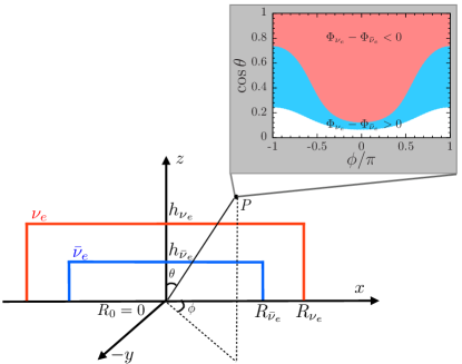
Figure 1: Geometry of $\nu_{e}$ (in red) and $\bar{\nu}_{e}$ (in blue) emitting surfaces with radii $R_{\nu_{e}}$ and $R_{\bar{\nu}_{e}}$, heights $h_{\nu_{e}}$ and $h_{\bar{\nu}_{e}}$. $R_{0}$ is the innermost stable circular orbit for a BH-disk system ($R_{0}=0$ for a NS-disk remnant). Inset: Example of crossings of the ELN distribution ($\Phi_{\nu_{e}}-\Phi_{\bar{\nu}_{e}}$) as a function of the polar and azimuthal angles $\cos\theta$ and $\phi$ above the NS–disk. The exact shapes are calculated at $(x,z)=(0.6R_{\nu_{e}},0.35R_{\nu_{e}})$ with $R_{\bar{\nu}_{e}}=0.75~{}R_{\nu_{e}}$ and $h_{\nu_{e}}/R_{\nu_{e}}=h_{\bar{\nu}_{e}}/R_{\bar{\nu}_{e}}=0.25$. The region shaded in red (blue) corresponds to $\Phi_{\nu_{e}}<\Phi_{\bar{\nu}_{e}}$ ($\Phi_{\nu_{e}}>\Phi_{\bar{\nu}_{e}}$).

III Dispersion relation in flavor space

The equation of motion (EoM) for each momentum mode governing the evolution of free streaming neutrinos is given by: $(\partial_{t}+\mathbf{v}\cdot\partial_{\mathbf{x}})\varrho=-i[H,\varrho]$ where $\mathbf{v}=(\sin\theta\cos\phi,\sin\theta\sin\phi,\cos\theta)$ is the velocity of an ultrarelativistic neutrino, whose 4-vector is $v^{\mu}=(1,\mathbf{v})$. The Wigner-transformed density matrix $\varrho$ in the flavor basis encodes the flavor occupation numbers in the diagonal terms and flavor correlations in the off-diagonal terms. The Hamiltonian, $H$, consists of the contributions from the vacuum mixing Patrignani et al. (2016), coherent-forward scattering between neutrinos and electrons, and that among neutrino themselves.

Dismissing the vacuum term and ignoring the energy dependence since we are interested in fast conversions, we express the neutrino density matrix in terms of the “flavor isospin” $\xi$ and the occupation numbers $f_{\nu_{\beta}}$ for the neutrino flavor $\nu_{\beta}$: $\varrho=[(f_{\nu_{e}}+f_{\nu_{x}})+(f_{\nu_{e}}-f_{\nu_{x}})\xi]/2$ ($\bar{\varrho}=-[(f_{\nu_{e}}+f_{\bar{\nu}_{x}})+(f_{\bar{\nu}_{e}}-f_{\bar{\nu}_{x}})\xi^{*}]/2$) for neutrinos (antineutrinos)  under the two-flavor mixing approximation. The Hamiltonian for $\xi(\mathbf{v})$ can be written as

$$H=v^{\mu}\lambda_{\mu}\frac{\sigma_{3}}{2}+\int d\Omega^{\prime}v^{\mu}v^{\prime}_{\mu}\xi(\mathbf{v}^{\prime})g(\mathbf{v}^{\prime})\ ,$$ (1)

where, given the metric $\eta^{\mu\nu}={\rm diag}(1,-1,-1,-1)$, $v^{\mu}\lambda_{\mu}=\lambda_{0}-\mathbf{v}\cdot\bm{\lambda}$ with $\lambda_{0}=\sqrt{2}G_{F}n_{e}$, $n_{e}$ being the net electron number density, $\bm{\lambda}=\lambda_{0}\mathbf{v_{f}}$, and $\mathbf{v_{f}}$ being the local fluid velocity. The neutrino potential angular distribution $g(\mathbf{v})$ per unit length per unit solid angle is proportional to the ELN angular distribution

$$g(\mathbf{v})\!=\!\sqrt{2}G_{F}\left(\Phi_{\nu_{e}}-\Phi_{\bar{\nu}_{e}}\right)\ .$$ (2)

$\Phi_{\nu_{\beta}}$ is related to the distribution functions $f_{\nu_{\beta}}$ by

$$\Phi_{\nu_{\beta}}(\mathbf{v})=\frac{dn_{\nu_{\beta}}(\mathbf{v})}{d\Omega}\!=\!\frac{1}{(2\pi)^{3}}\int dEE^{2}f_{\nu_{\beta}}(E,\mathbf{v})\ ,$$ (3)

with $d\Omega=d\cos\theta d\phi$ the differential solid angle. Since we work in the corotating frame of the disk, the term $\mathbf{v}\cdot\bm{\lambda}$ will be neglected from now on.

In order to investigate whether off-diagonal terms may originate in the density matrix giving rise to fast conversions, we now linearize the EoM Banerjee et al. (2011); Raffelt et al. (2013) and track the evolution of the off-diagonal term $S$ in $\xi$,

$$\xi=\left(\begin{matrix}1&S\\ S^{*}&-1\\ \end{matrix}\right),$$ (4)

by neglecting terms larger than $\mathcal{O}(|S|)$. Assuming that $S(\mathbf{v})$ evolves as a plane wave $S(\mathbf{v},t,{\mathbf{x}})=Q(\mathbf{v},\omega,\mathbf{k})e^{-i(\omega t-{\mathbf{k}}\cdot{\mathbf{x}})}$, the EoM becomes Izaguirre et al. (2017)

$$v_{\mu}s^{\mu}Q(\mathbf{v},\omega,\mathbf{k})+\int d\Omega^{\prime}v_{\mu}v^{\prime\mu}g(\mathbf{v}^{\prime})Q(\mathbf{v^{\prime}},\omega,\mathbf{k})=0\ ,$$ (5)

by defining the 4-vector $s^{\mu}\equiv(\omega-\lambda_{0}-\epsilon_{0},\mathbf{k}-\bm{\epsilon})$, $\epsilon_{0}\equiv\int d\Omega g(\mathbf{v})$ and $\bm{\epsilon}\equiv\int d\Omega g(\mathbf{v})\mathbf{v}$. From the structure of Eq. (5), one sees that the solution of $Q(\mathbf{v},\omega,\mathbf{k})$ has the form of $(v_{\mu}a^{\mu})/(v_{\mu}s^{\mu})$. A nontrivial $a^{\mu}$ exists, if

$${\rm det}[\Pi_{\mu\nu}(\omega,\mathbf{k})]=0\ ,$$ (6)

where $\Pi_{\mu\nu}(\omega,\mathbf{k})=\eta_{\mu\nu}+\int d\Omega\ v_{\mu}v_{\nu}g(\mathbf{v})/(v_{\mu}s^{\mu})$.

Equation (6) is the DR for the mode with $(\omega,\mathbf{k})$ Izaguirre et al. (2017). If the solutions satisfying the DR consist of real $(\omega,\mathbf{k})$ only, any initial perturbations in the flavor space do not grow in the linear regime. If, however, any conjugate pair of complex solutions in $\omega$ or $k_{i}$ ($i\in\{x,y,z\}$) satisfies the DR, an instability growing exponentially with rate $|{\rm Im}(\omega)|$ or $|{\rm Im}(k_{i})|$ occurs, leading to flavor conversions. Practically, one examines whether the system is temporally (spatially) unstable by finding all solutions of $\omega$ ($k_{i}$) with a given $\mathbf{k}$ ($\omega$ and $k_{j\neq i}$) Izaguirre et al. (2017).

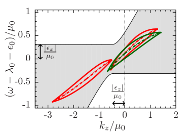
Figure 2: Dispersion relation of $\mathbf{k}=(0,0,k_{z})$ for the ELN distribution shown in Fig. 1 with $\alpha=\Phi^{0}_{\bar{\nu}_{e}}/\Phi^{0}_{\nu_{e}}=2.4$. For the complex $\omega$ that lead to flavor instability, ${\rm Re}(\omega)$ are shown by the red (green) dash-dotted curves and ${\rm Re}(\omega)\pm{\rm Im}(\omega)$ are shown by the red (green) solid curves for the MS preserving (breaking) solutions. The gray regions are the zone of avoidance for real $(\omega,k_{z})$. The temporal instability exists for a large range of $k_{z}/\mu_{0}$ and it is, therefore, unavoidable.

IV Temporal instabilities above the remnants

Motivated by the crossings of the local ELN distribution resulting from the disk emission geometry and the protonization of the merger remnant, we now investigate conditions for temporal instabilities above the NS–disk system. To this purpose, we examine the solution of the DR for the ELN distribution at the location $(x,z)=(0.6~{}R_{\nu_{e}},0.35~{}R_{\nu_{e}})$ above the NS–disk system shown in Fig. 1 as a benchmark case. We note that any generic point above the $\nu_{e}$-emitting surface would exhibit qualitatively similar solutions for the DR (see also Appendix A for $g(\mathbf{v})$ distributions at different locations), despite the relative contribution of $\nu_{e}$ and $\bar{\nu}_{e}$ to $g(\mathbf{v})$ varies significantly at different locations. This is because the features responsible for inducing flavor conversions (i.e., the change of sign in $g(\mathbf{v})$) are present everywhere above the remnant and cannot be avoided differently from the SN case.

First, we solve the DR equation for the modes $\mathbf{k}=(0,0,k_{z})$ and $\alpha\equiv\Phi^{0}_{\bar{\nu}_{e}}/\Phi^{0}_{\nu_{e}}=2.4$. Due to the mirror symmetry (MS) with respect to the $y$ axis, Eq. (6) has $\Pi_{02}=\Pi_{12}=\Pi_{32}=0$ and it reduces to

$$\Pi_{22}(-\Pi_{03}^{2}\Pi_{11}+2\Pi_{01}\Pi_{03}\Pi_{13}-\Pi_{00}\Pi_{13}^{2}-\Pi_{33}\Pi_{01}^{2}$$

$$+\Pi_{00}\Pi_{11}\Pi_{33})=0.$$ (7)

An ${\rm Im}(\omega)\neq 0$ from $\Pi_{22}=0$ corresponds to a MS breaking unstable solution. When the terms inside the parentheses sum to 0, a MS-preserving solution occurs instead.

Figure 2 shows the temporal DR for the benchmark location. We define $\mu_{0}=\sqrt{2}G_{F}n^{0}_{\nu_{e}}$ to denote a typical length scale,

$$\mu_{0}\approx 4.25\ {\rm cm}^{-1}\left(\frac{L_{\nu_{e}}}{10^{53}{\rm erg/s}}\right)\left(\frac{10{\rm MeV}}{\langle E_{\nu_{e}}\rangle}\right)\left[\frac{(100{\rm km})^{2}}{R_{\nu_{e}}^{2}-R_{0}^{2}}\right]\ ,$$ (8)

with $L_{\nu_{e}}$ the total energy luminosity of $\nu_{e}$, $\langle E_{\nu_{e}}\rangle$ the corresponding average energy. A temporal instability generally exists for a large range of $|k_{z}|/\mu_{0}$ (i.e., $|k_{z}|\simeq$ a few times $\mu_{0}$), centered around $k_{z}\approx\epsilon_{z}=-0.46~{}\mu_{0}$.

Because of the broken axial symmetry, we find three branches of the unstable solutions: two of them preserving the $y$-MS (red curves) and the other one breaking this symmetry (green curves). No real solutions exist for the selected $(x,z)$ due to the enlarged zone of avoidance (gray region), where $Q(\mathbf{v})$ would become singular as a result of larger asymmetry in the $x$ direction ($|\epsilon_{x}|=0.31\mu_{0}$). Note that, for $g(\mathbf{v})$ corresponding to other $(x,z)$ above the $\nu_{e}$ surface, we find nonzero real solution(s) that sometimes coexist with the complex ones because of the disk geometry, differently from the findings of Ref. Izaguirre et al. (2017).

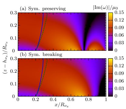
Figure 3: Contour plot of $|{\rm Im}(\omega)|/\mu_{0}$ in the $(x,z)$ plane above the $\nu_{e}$-surface for $\mathbf{k}=0$ for our benchmark NS-disk model. The mirror symmetry preserving and breaking solutions are shown in panel (a) and (b). Also shown are the MNR locations obtained by adopting the $n_{e}$ profiles of Perego et al. (2014) for neutrinos emitted at $(x,z)=(0,h_{\nu_{e}})$ (solid blue curve) and at $(x,z)=(-R_{\nu_{e}},h_{\nu_{e}})$ (dashed green curve). Fast conversions occur everywhere above the $\nu_{e}$ surface and could alter the otherwise favorable conditions for the MNR.

So far, we have focused on the temporal instabilities for one specific point $(x,z)$ above the $\nu_{e}$ surface of the NS disk. Since the $k_{z}=0$ mode is unstable in this studied case, we adopt it as the benchmark wave number and generalize our study to any $(x,z)$ above the $\nu_{e}$ emitting disk surface. Figure 3 shows contour plots of the growth rate $|\mathrm{Im}(\omega_{0})|/\mu_{0}$ in the $(x,z)$ plane. MS preserving (panel(a)) and breaking (panel(b)) flavor instabilities exist in most of the region above the $\nu_{e}$ surface. Moreover, $|\mathrm{Im}(\omega_{0})|/\mu_{0}$ at some vertical distance above the $\nu_{e}$ surface may be larger than that at the surface. The growth rate $|{\rm Im}(\omega)|$ is typically large $\sim 0.1\mu_{0}$, leading to flavor conversion in the length scale of cm.

The eventual occurrence of fast conversions above the $\nu_{e}$ emitting surface hints towards a change of paradigm of the current picture of flavor conversions in merger remnants, in particular concerning the occurrence of the MNR. In fact, in Fig. 3 we also show the locations of the MNR for neutrinos emitted from the center ($x=0,z=h_{\nu_{e}}$, solid blue curve) and the opposite side of the disk ($x=-R_{\nu_{e}},z=h_{\nu_{e}}$, dashed green curve), using the $n_{e}$ profiles from (Perego et al., 2014) to model the matter potential. Before these neutrinos reach the MNR locations, they will traverse the region where the fast conversions can occur and this would likely alter the MNR conditions.

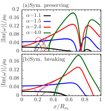
Figure 4: Growth rate of the flavor instability, $|{\rm Im}(\omega)|/\mu_{0}$, as a function of $x$ on the $\nu_{e}$-surface for the same NS disk in Fig. 1 (thick curves) with different $\alpha=\Phi^{0}_{\bar{\nu}_{e}}/\Phi^{0}_{\nu_{e}}$ for the mirror symmetry preserving solutions [panel (a)] and the mirror symmetry breaking solutions [panel (b)]. The thin dashed curves show the corresponding solutions of the BH torus with $R_{0}=0.15R_{\nu_{e}}$. For any $\alpha\geq 1.1$, flavor instabilities exist above the $\nu_{e}$ surface.

In order to further generalize our results to any $\alpha$ compatible with existing hydrodynamical simulations, Fig. 4 shows the temporal instability of $\mathbf{k}=0$ for the same disk model with different values of the flux ratio $\alpha=1.1$, 1.5, 2.4, and 4.0 covering the range of $(L_{\bar{\nu}_{e}}/\langle E_{\bar{\nu}_{e}}\rangle)/(L_{\nu_{e}}/\langle E_{\nu_{e}}\rangle)$ from hydrodynamical simulations listed in Table 7 of Ref. Frensel et al. (2017). For this wide range of $\alpha$, MS preserving and breaking flavor instabilities are found in most of the region right above the $\nu_{e}$ surface. As one moves from the disk center towards the edge, the MS preserving unstable solution shifts from one branch to another (see Figs. 2 and 3), and there is a small region where no MS preserving unstable solution exists. Nevertheless, the MS breaking unstable solution is nonzero in this region. We conclude that fast conversions can occur in most of the region above the merger remnant of the NS disks for any realistic $\alpha$.

For the remnant system consisting of a central BH and an accretion disk, we show in Fig. 4 the corresponding temporal instability with thin dashed curves for $R_{0}=0.15~{}R_{\nu_{e}}$ for both $\nu_{e}$ and $\bar{\nu}_{e}$ emitting tori (see Fig. 1 and Appendix A for details). The growth rates are different in the proximity of $R_{0}$, but for $x\gtrsim 0.4R_{\nu_{e}}$, they coincide with the values in the NS–disk ($R_{0}=0$) cases. Note that close to $R_{0}$, the growth rates might be even enhanced due to the suppressed $\bar{\nu}_{e}$ phase space in our simple toy model.

V Spatial instabilities above the remnants

Similarly to the temporal instabilities discussed in Sec. IV, the ELN crossings can also lead to the occurrence of spatial instabilities (Dasgupta et al., 2017; Izaguirre et al., 2017). However, differently from the temporal instabilities whose growth rate does not depend on the adopted matter density profile, the matter density has strong impact on the occurrence of spatial instabilities (Chakraborty et al., 2016b; Dasgupta et al., 2017).

To study spatial instabilities in the compact binary merger remnants, we adopt the same NS–disk neutrino emission model as in Sec. IV and the cylindrically-averaged electron number density profile $n_{e}(x,z)$ from Ref. (Perego et al., 2014) at 60 ms post merger. As we will show later, spatial instabilities are more likely to occur in the low-density polar region above the disk, therefore we choose the location $(x,z)=(0,0.25R_{\nu_{e}})$ on the $\nu_{e}$ emitting surface as a benchmark example to study the DR for the occurrence of spatial instabilities.

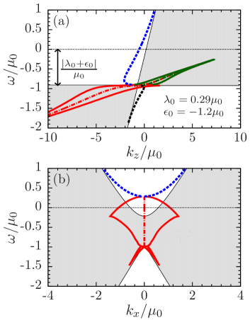
Figure 5: Dispersion relation of $(\omega,\mathbf{k})=(\omega,0,0,k_{z})$ [panel(a)] and $(\omega,k_{x},0,0)$ [panel(b)] for the ELN distribution at $(x,z)=(0,0.25R_{\nu_{e}})$ with $\alpha=\Phi^{0}_{\bar{\nu}_{e}}/\Phi^{0}_{\nu_{e}}=2.4$ (see top left panel of Fig. 9). For the complex $k_{z,x}$ that lead to the spatial flavor instability, ${\rm Re}(k_{z,x})$ are shown by the red (green) dash-dotted curves and ${\rm Re}(k_{z,x})\pm{\rm Im}(k_{z,x})$ are shown by the red (green) solid curves for the MS preserving (breaking) solutions. The gray regions are zone of avoidance for real $(\omega,k_{z,x})$.

Figure 5 shows the $k_{z}$ ($k_{x}$) solution of DR as a function of $\omega$ for a mode with $k_{x}=k_{y}=0$ ($k_{z}=k_{y}=0$) for the NS–disk system with $\alpha=2.4$.

Since the spatially unstable solutions usually exist at $|\omega-\lambda_{0}-\epsilon_{0}|\lesssim\mu_{0}$, a large $\lambda_{0}+\epsilon_{0}$ can suppress the instability for a mode with $\omega=0$ as shown in the panel (a) of Fig. 5, in which the mode propagating at the $z$ direction with $\omega=k_{x}=k_{y}=0$ is stable. (This is mainly due to $\epsilon_{0}$, similarly to the multiangle self-suppression (Duan and Friedland, 2011; Banerjee et al., 2011).)

However, this depends on the propagating mode that one is examining. For example, panel (b) shows that, at the same location, a spatial instability can exist for the mode propagating in the $x$ direction with $\omega=k_{z}=k_{y}=0$. This is due to the fact that neutrinos travel in all $\phi$ directions above the disk, therefore providing enough transverse flux for the spatial instabilities to occur . Moreover, even though the propagating mode with $\omega=0$ can be stable with respect to spatial instabilities in some cases, if there exists a highly oscillatory perturbation in the mode with $\omega\approx\lambda_{0}+\epsilon_{0}$, the system can always be unstable due to the ELN crossing (see previous section).

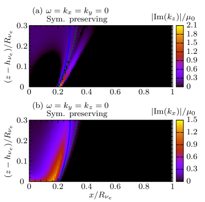
Figure 6: Contour plot of the mirror symmetry preserving solution of $|{\rm Im}(k_{z})|/\mu_{0}$ [panel(a)] and $|{\rm Im}(k_{x})|/\mu_{0}$ [panel(b)] in the $(x,z)$ plane above the $\nu_{e}$-surface for $\omega=k_{x}=k_{y}=0$ and $\omega=k_{z}=k_{y}=0$ for the NS-disk model with $\alpha=2.4$, using the $n_{e}$ profiles of Perego et al. (2014) at 60 ms post merger. Also shown are the MNR locations for neutrinos emitted at $(x,z)=(0,h_{\nu_{e}})$ (solid blue curve) and at $(x,z)=(-R_{\nu_{e}},h_{\nu_{e}})$ (dashed green curve). The spatial instabilities exist inside the low-density funnel where $\lambda_{0}\lesssim|\epsilon_{0}|$ and are largely suppressed outside the funnel where $\lambda_{0}\gg|\epsilon_{0}|$.

Now let us look at how the spatial instabilities depend on the location above the disk. Above the NS–disk, the angular momentum of the system keeps the density in the region close to the $z$ axis much lower compared to the off-axis parts (see, e.g., Fig. 1 of Ref. (Frensel et al., 2017)). Therefore, the occurrence of spatial instabilities sensitively depends on the location above the disk. Figure 6 shows the $y$-MS preserving instabilities of the propagating modes with $\omega=k_{x}=k_{y}=0$ and $\omega=k_{z}=k_{y}=0$ above the $\nu_{e}$-surface.

In the outer region above the disk, spatial instabilities are suppressed by the large matter potential, $\lambda_{0}\gg|\epsilon_{0}|$. Inside the low-density funnel, where $\lambda_{0}\lesssim|\epsilon_{0}|$, the $k_{z}$ instability only exists where $\lambda_{0}\sim\epsilon_{0}$, close to the MNR region. However, the propagating $k_{x}$ modes can be unstable everywhere inside the low-density funnel.

Because the instabilities only occur in the inner region above the disk, the breaking of the local MS symmetry is minor. Therefore, the unstable $k_{y}$ solutions and the MS breaking $k_{x}$ solutions are very similar to the $k_{x}$ MS preserving solutions and therefore are not discussed here.

We note that the growth rate of the spatial instabilities is generally larger than the temporal instabilities discussed in Sec. IV. This suggests that in order to fully grasp how flavor conversion develops above the disk in the nonlinear regime, numerical simulations that evolve simultaneously in time and space coordinates are necessary.

VI Discussion

Within our simplified two-neutrino-emission disks model, we have shown that both temporal and spatial instabilities can exist above the remnants of compact binary mergers. This is a direct consequence of the larger local antineutrino emissivity compared to the neutrino one as well as of the spatial separation of their respective emission surfaces.

In a more realistic environment, the matter density profile along the $z$ direction would decrease much faster on the surface of the central massive neutron star and in the inner part of the disk. As a consequence, the separation between $\nu_{e}$ and $\bar{\nu}_{e}$ in the inner disk region would be smaller than in the outer region. However, one should still expect an overall more extended $\nu_{e}$ surface with respect to the $\bar{\nu}_{e}$ one in the outer region as a result of the spatial extension of the accretion disk.

In order to investigate whether the above effect could modify our main findings, we have examined the occurrence of instabilities in an extreme scenario in which the heights of $\nu_{e}$ and $\bar{\nu}_{e}$ emission surfaces are the same. As an example, Fig. 7 shows the $y$-MS preserving solution of $|{\rm Im}(\omega)|/\mu_{0}$ in the $(x,z)$ plane above the $\nu_{e}$ surface for $\mathbf{k}=0$ for a NS–disk model with $h_{\nu_{e}}=h_{\bar{\nu}_{e}}=0.25R_{\nu_{e}}$, $R_{\bar{\nu}_{e}}=0.75R_{\nu_{e}}$, and $\alpha=2.4$. In this case, the temporal instability in the central part right above the disk can be suppressed (see Fig. 3 with $h_{\bar{\nu}_{e}}=0.75h_{\nu_{e}}$ for comparison). This is because of the reduced $\nu_{e}$ dominated part of the ELN distribution very close to the inner part of $\nu_{e}$ emission surface.

Far away from the surface in Fig. 3, where the spatial extension of the disks becomes important, favorable conditions for temporal instability are however recovered. Furthermore, the spatial instabilities for the transversely propagating mode can always exist. Thus, we conclude that even taking into account a more realistic neutrino emission geometry, flavor instabilities leading to fast pairwise conversion exist in an extended region above the merger remnants.

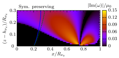
Figure 7: Symmetry preserving solution of $|{\rm Im}(\omega)|/\mu_{0}$ in the $(x,z)$ plane above the $\nu_{e}$-surface for $\mathbf{k}=0$ for the same NS-disk model as in Fig. 3 except for that $h_{\nu_{e}}=h_{\bar{\nu}_{e}}=0.25R_{\nu_{e}}$. The temporal instability in the central part right above the disk is suppressed, see Fig. 3 for comparison.

In a realistic astrophysical environment, a non-negligible flux of neutrinos streaming in the negative $z$ direction exists because of collisions. This may also be responsible for fast flavor conversions Chakraborty et al. (2016b); Dasgupta et al. (2017); Izaguirre et al. (2017). Given the still preliminary neutrino transport employed in merger simulations with respect to SN simulations, we refrain from including any backward contribution in our toy-model. In fact, given the favorable conditions for fast flavor conversions determined by the ubiquitous crossings of ELN distribution, any contribution due to neutrino collisions would further strengthen our conclusions.

Likewise, hydrodynamical simulations would predict location-dependent neutrino emissivities, forward-peaked neutrino angular distributions on their emission surfaces (instead of the uniform distributions adopted here), and time-dependent neutrino properties due to the long-term evolution of the remnant system. Those effects, not considered in our simple model, can all quantitatively influence the exact conditions responsible for fast conversions. However, we expect the qualitative features presented here will be unchanged.

VII Conclusions

NS–NS and NS–BH compact mergers are neutrino-dense sources. For the first time, we investigate the role of the neutrino angular distributions in flavor conversions in merger remnant disks and explore the occurrence of fast flavor conversions. Given the current uncertainties on the modeling of the neutrino transport in merger remnants, we do not rely on direct inputs from a specific hydrodynamical simulation and, instead, model the local neutrino radiation field using a simple two-neutrino-emitting surfaces model whose parameters are guided by (Perego et al., 2014). We then adjust the model parameters to cover the range spanned by existing hydrodynamical simulations and obtain reliable results.

Because of the larger $\bar{\nu}_{e}$ flux with respect to the $\nu_{e}$ one, and the emission geometry of the disk, crossings between the $\nu_{e}$ and $\bar{\nu}_{e}$ angular distributions are present for any point above the merger disk remnant, differently from SNe, where crossings do not occur unless strong directional-dependent neutrino emission is invoked due to the multidimensional effects. Consequently, we showed in Sec. IV that fast flavor conversions caused by temporal disturbances may be intrinsically unavoidable in compact mergers remnants.

We also discussed the presence of spatial instabilities in Sec. V. Those are sensitive to the model-dependent matter density profile and to the transversally propagating neutrinos. Favorable conditions for those instabilities, with growth rates larger than the temporal instabilities, appear above merger remnants. Nevertheless, spatial instabilities occur in smaller spatial regions than the temporal ones due to the partial matter suppression effect (unless initial perturbations exists in $\omega\approx\lambda_{0}+\epsilon_{0}$ not studied in this work). The presence of any spatial instabilities would make the system, already suffering unavoidable temporal instabilities, even more unstable. Hence, it is necessity to take into account both temporal and spatial evolution of flavor conversion in upcoming numerical studies.

A more realistic shape of neutrino emitting surfaces may certainly affect the results obtained within our simple two-disks model quantitatively. In Sec. VI, we discussed the potential impact and showed that our conclusions should be qualitatively fairly general despite that the two-disk neutrino emission model is highly simplified.

The stability analysis presented in this paper proves that favorable conditions for fast flavor conversions can exist in mergers. However, similarly to the case of core-collapse supernovae, we still miss an exact numerical solution of the neutrino flavor evolution. Our preliminary results suggest that fast flavor conversions should be taken seriously in compact merger remnants as they may lead to flavor equilibration very close to the neutrino decoupling region.

Flavor equilibration in the neutrino decoupling region could be responsible for nontrivial modifications of the jet dynamics, if powered by neutrinos, as well as of the production of heavy elements. For example, it could largely reduce the neutrino pair annihilation rate above a BH-torus remnant Ruffert et al. (1997); Foucart et al. (2015). Similarly, it could also change the composition of the ejecta exposed to neutrinos Wanajo et al. (2014); Metzger and Fernández (2014); Perego et al. (2014). This will modify the predicted $r$-process outcome and the associated kilonova light curves in merger events. Given that the relevant length scales induced by fast conversions are much smaller than the resolution of merger simulations, the impact of pairwise conversions should be phenomenologically explored. In addition, as a consequence of our findings, the adopted picture of the MNR occurring in merger remnants should be revised, and future work is needed in this direction.

Appendix A Emission geometry of the two-disks neutrino model

The toy-model adopted to simulate the neutrino emission from compact binary merger remnants is here described in detail. The local neutrino radiation field is also characterized for any point above the emitting surface.

The neutrino decoupling region has been approximated by flavor-dependent emitting surfaces shown in Fig. 1. For the sake of simplicity, we assume that the (energy-integrated) angular distribution on each $\nu$ surface is half-isotropic with $\Phi_{\nu_{\beta}}^{0}=dn_{\nu_{\beta}}^{0}/d\Omega=L_{\nu_{\beta}}/[2\pi^{2}(R_{\nu_{\beta}}^{2}-R_{0}^{2})\langle E_{\nu_{\beta}}\rangle]$ for $\cos\theta\geq 0$, $R_{0}\leq\sqrt{x^{2}+y^{2}}\leq R_{\nu_{\beta}}$ at $z=h_{\nu_{\beta}}$, where $L_{\nu_{\beta}}$ is the total energy luminosity of $\nu_{\beta}$ and $\langle E_{\nu_{\beta}}\rangle$ is the corresponding average energy. The choice of the model parameters is guided by the hydrodynamical simulation of the massive NS–disk evolution as a remnant of a NS–NS merger Perego et al. (2014): $R_{\bar{\nu}_{e}}=0.75R_{\nu_{e}}$, $h_{\nu_{e}}/R_{\nu_{e}}=h_{\bar{\nu}_{e}}/R_{\bar{\nu}_{e}}=0.25$, and $\alpha\equiv\Phi^{0}_{\bar{\nu}_{e}}/\Phi^{0}_{\nu_{e}}=2.4$.

At a given location, $P\equiv(x,z)$, above the neutrino emitting surfaces depicted in Fig. 1, $g(\mathbf{v})$ can be rewritten as

$$g(\mathbf{v})=\sqrt{2}G_{F}[\Phi^{0}_{\nu_{e}}\zeta_{\nu_{e}}(\mathbf{v})-\Phi^{0}_{\bar{\nu}_{e}}\zeta(\mathbf{v})]\ ,$$ (9)

where $\zeta_{\nu_{\beta}}(\mathbf{v})=1$ for any $\mathbf{v}$ that can be traced back to the corresponding $\nu_{\beta}$-emitting surfaces and 0 otherwise.

For the NS–disk $(R_{0}=0)$, the ranges of $\theta\in[\theta_{\rm min},\theta_{\rm max}]$ and $\phi\in[-\phi_{\rm max},\phi_{\rm max}]$ in which $\zeta_{\nu_{\beta}}(\mathbf{v})=1$ can be derived straightforwardly and are shown in Fig. 8 (top panel). They are defined by

$$\cos\phi_{\rm max}=\begin{cases}-1&0\leq x<R_{\nu_{\beta}}\\ \dfrac{\sqrt{x^{2}-R_{\nu_{\beta}}^{2}}}{x}&x\geq R_{\nu_{\beta}}\ ,\end{cases}$$ (10a)

$$\tan{\theta_{\rm min}}=\begin{cases}0&0\leq x<R_{\nu_{\beta}}\\ \dfrac{x\cos\phi-\sqrt{R_{\nu_{\beta}}^{2}-x^{2}\sin^{2}\phi}}{z-h_{\nu_{\beta}}}&x\geq R_{\nu_{\beta}}\ ,\end{cases}$$ (10b)

$$\tan\theta_{\rm max}=\frac{x\cos\phi+\sqrt{R_{\nu_{\beta}}^{2}-x^{2}\sin^{2}\phi}}{z-h_{\nu_{\beta}}}\ .$$ (10c)

Note that $\theta_{\rm min}$ and $\theta_{\rm max}$ are functions of $\phi$.

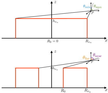
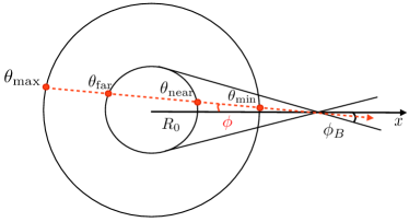
Figure 8: Angular projections for neutrinos emitted from the disk surface. Top panel: The neutrino distribution at a point $P$ at a certain distance from the NS-disk surface is restricted within the angles $\theta_{\rm min}$ and $\theta_{\rm max}$ for a certain $\phi$ [see Eq. (10)]. Middle panel: Same as above but for a BH-disk surface. The neutrino distribution at $P$ also depend on $\phi$. In this example, neutrinos can only reach $P$ from $\theta_{\rm min}\leq\theta\leq\theta_{\rm near}$ and $\theta_{\rm far}\leq\theta\leq\theta_{\rm max}$, see Eq. (11). Bottom panel: Angular projections for the BH-disk viewed from above, see text for details.

For the BH–torus, the corresponding values of $\phi_{\rm max}$ are the same as in the above equations. On the other hand, the range of $\theta$ for $x\geq R_{0}$ becomes more complicated. Given the configuration of the emitting surface shown in Fig. 8 (middle panel), for $\phi\geq\phi_{B}=\arccos(\sqrt{x^{2}-R_{0}^{2}}/x)$ or $\phi\leq-\phi_{B}$, $\zeta_{\nu_{\beta}}(\mathbf{v})=1$ for $\theta\in[\theta_{\rm min},\theta_{\rm max}]$. Similarly, for $-\phi_{B}<\phi<\phi_{B}$, $\zeta_{\nu_{\beta}}(\mathbf{v})=1$ for $\theta\in[\theta_{\rm min},\theta_{\rm near}]$ and $\theta\in[\theta_{\rm far},\theta_{\rm max}]$ with

$$\tan{\theta_{\rm near}}=\frac{x\cos\phi-\sqrt{R_{0}^{2}-x^{2}\sin^{2}\phi}}{z-h_{\nu_{\beta}}}\ ,$$ (11a)

$$\tan{\theta_{\rm far}}=\frac{x\cos\phi+\sqrt{R_{0}^{2}-x^{2}\sin^{2}\phi}}{z-h_{\nu_{\beta}}}\ .$$ (11b)

See also the bottom panel of Fig. 8 for details.

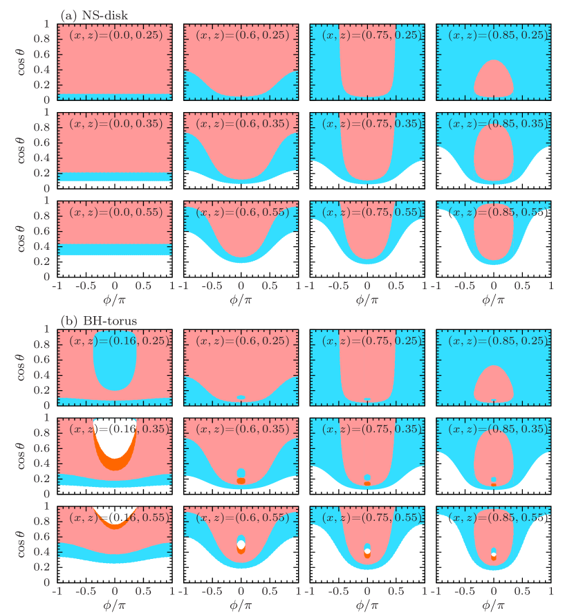
Figure 9: Electron neutrino lepton number distribution, $\Phi_{\nu_{e}}-\Phi_{\bar{\nu}_{e}}$, as a function of $\cos\theta$ and $\phi$ and different $(x,z)$ points above the $\nu_{e}$ surface. The top three rows [panel (a)] refer to our benchmark NS–disk model ($R_{\bar{\nu}_{e}}=0.75R_{\nu_{e}}$ $h_{\nu_{e}}/R_{\nu_{e}}=h_{\bar{\nu}_{e}}/R_{\bar{\nu}_{e}}=0.25$, and $\alpha\equiv\Phi^{0}_{\bar{\nu}_{e}}/\Phi^{0}_{\nu_{e}}>1$). In the red (blue) shaded area, $\Phi_{\nu_{e}}-\Phi_{\bar{\nu}_{e}}<0$ ($\Phi_{\nu_{e}}-\Phi_{\bar{\nu}_{e}}>0$). Null electron neutrino lepton number is shown in white. The bottom three rows [panel (b)] refer to the BH–torus case with $R_{0}=0.15R_{\nu_{e}}$ and the orange shaded area marks regions where $\Phi_{\nu_{e}}=0$. In both cases, as one moves away from the surface center, the $\bar{\nu}_{e}$ contribution is significantly reduced.

As an illustrative example, $\Phi_{\nu_{e}}-\Phi_{\bar{\nu}_{e}}=[\Phi^{0}_{\nu_{e}}\zeta_{\nu_{e}}(\mathbf{v})-\Phi^{0}_{\bar{\nu}_{e}}\zeta(\mathbf{v})]$ as a function of $\cos\theta$ and $\phi$ is shown in Fig. 9 for the same NS–disk model of Fig. 1 (panel (a), top three rows) and for the BH–torus model (panel (b), bottom three rows). A set of $(x,z)$ locations is plotted for both the NS and BH cases. In the red shaded area, $g(\mathbf{v})<0$ [$\zeta_{\nu_{e}}(\mathbf{v})=\zeta_{\bar{\nu}_{e}}(\mathbf{v})=1$] for $\Phi^{0}_{\bar{\nu}_{e}}/\Phi^{0}_{\nu_{e}}>1$. In the blue area, $g(\mathbf{v})>0$ [$\zeta_{\bar{\nu}_{e}}(\mathbf{v})=0$] . In the white area, $g(\mathbf{v})=0$ and in the orange area $\zeta_{\nu_{e}}(\mathbf{v})=0$. Figure 9 shows that as one moves away from the surface center, the $\bar{\nu}_{e}$ contribution can be significantly reduced and $g(\mathbf{v})=0$ for a certain range of $\cos\theta$ and $\phi$. In the BH–torus ($R_{0}\neq 0$), white holes appear in $g(\mathbf{v})$ as well as regions only populated by $\bar{\nu}_{e}$ because of the toroidal geometry described above.

References

- Eichler et al. (1989) D. Eichler, M. Livio, T. Piran, and D. N. Schramm, Nature 340, 126 (1989).
- Berger (2014) E. Berger, Ann. Rev. Astron. Astrophys. 52, 43 (2014), eprint 1311.2603.
- Metzger et al. (2010) B. D. Metzger, G. Martínez-Pinedo, S. Darbha, E. Quataert, A. Arcones, D. Kasen, R. Thomas, P. Nugent, I. V. Panov, and N. T. Zinner, Mon. Not. Roy. Astron. Soc. 406, 2650 (2010), eprint 1001.5029.
- Tanvir et al. (2013) N. R. Tanvir, A. J. Levan, A. S. Fruchter, J. Hjorth, K. Wiersema, R. Tunnicliffe, and A. de Ugarte Postigo, Nature 500, 547 (2013), eprint 1306.4971.
- Yang et al. (2015) B. Yang, Z.-P. Jin, X. Li, S. Covino, X.-Z. Zheng, K. Hotokezaka, Y.-Z. Fan, T. Piran, and D.-M. Wei, Nature Commun. 6, 7323 (2015), eprint 1503.07761.
- Lattimer and Schramm (1974) J. M. Lattimer and D. N. Schramm, Astrophys. J. 192, L145 (1974).
- Freiburghaus et al. (1999) C. Freiburghaus, S. Rosswog, and F.-K. Thielemann, Astrophys. J. 525, L121 (1999).
- Abbott et al. (2016a) B. P. Abbott et al. (Virgo, LIGO Scientific), Phys. Rev. Lett. 116, 061102 (2016a), eprint 1602.03837.
- Abbott et al. (2016b) B. P. Abbott et al. (Virgo, LIGO Scientific), Phys. Rev. Lett. 116, 241103 (2016b), eprint 1606.04855.
- Ruffert et al. (1997) M. Ruffert, H.-T. Janka, K. Takahashi, and G. Schaefer, Astron. Astrophys. 319, 122 (1997), eprint astro-ph/9606181.
- Foucart et al. (2015) F. Foucart, E. O’Connor, L. Roberts, M. D. Duez, R. Haas, L. E. Kidder, C. D. Ott, H. P. Pfeiffer, M. A. Scheel, and B. Szilagyi, Phys. Rev. D91, 124021 (2015), eprint 1502.04146.
- Perego et al. (2014) A. Perego, S. Rosswog, R. M. Cabezón, O. Korobkin, R. Käppeli, A. Arcones, and M. Liebendörfer, Mon. Not. Roy. Astron. Soc. 443, 3134 (2014), eprint 1405.6730.
- Sadowski et al. (2008) A. Sadowski, K. Belczynski, T. Bulik, N. Ivanova, F. A. Rasio, and R. W. O’Shaughnessy, Astrophys. J. 676, 1162 (2008), eprint 0710.0878.
- Abbott et al. (2016c) B. P. Abbott et al. (Virgo, LIGO Scientific), Astrophys. J. 832, L21 (2016c), eprint 1607.07456.
- Wanajo et al. (2014) S. Wanajo, Y. Sekiguchi, N. Nishimura, K. Kiuchi, K. Kyutoku, and M. Shibata, Astrophys. J. 789, L39 (2014), eprint 1402.7317.
- Metzger and Fernández (2014) B. D. Metzger and R. Fernández, Mon. Not. Roy. Astron. Soc. 441, 3444 (2014), eprint 1402.4803.
- Birkl et al. (2007) R. Birkl, M. A. Aloy, H.-T. Janka, and E. Müller, Astron. Astrophys. 463, 51 (2007), eprint astro-ph/0608543.
- Zalamea and Beloborodov (2011) I. Zalamea and A. M. Beloborodov, Mon. Not. Roy. Astron. Soc. 410, 2302 (2011), eprint 1003.0710.
- Richers et al. (2015) S. Richers, D. Kasen, E. O’Connor, R. Fernández, and C. D. Ott, Astrophys. J. 813, 38 (2015), eprint 1507.03606.
- Just et al. (2016) O. Just, M. Obergaulinger, H. T. Janka, A. Bauswein, and N. Schwarz, Astrophys. J. 816, L30 (2016), eprint 1510.04288.
- Wolfenstein (1978) L. Wolfenstein, Phys. Rev. D17, 2369 (1978).
- Mikheyev and Smirnov (1985) S. P. Mikheyev and A. Yu. Smirnov, Sov. J. Nucl. Phys. 42, 913 (1985), [Yad. Fiz.42,1441(1985)].
- Fuller et al. (1987) G. M. Fuller, R. W. Mayle, J. R. Wilson, and D. N. Schramm, Astrophys. J. 322, 795 (1987).
- Pantaleone (1992) J. T. Pantaleone, Phys.Lett. B287, 128 (1992).
- Sigl and Raffelt (1993) G. Sigl and G. Raffelt, Nucl.Phys. B406, 423 (1993).
- Duan et al. (2010) H. Duan, G. M. Fuller, and Y.-Z. Qian, Ann. Rev. Nucl. Part. Sci. 60, 569 (2010), eprint 1001.2799.
- Duan (2015) H. Duan, Int. J. Mod. Phys. E24, 1541008 (2015), eprint 1506.08629.
- Mirizzi et al. (2016) A. Mirizzi, I. Tamborra, H.-T. Janka, N. Saviano, K. Scholberg, R. Bollig, L. Hudepohl, and S. Chakraborty, Riv. Nuovo Cim. 39, 1 (2016), eprint 1508.00785.
- Chakraborty et al. (2016a) S. Chakraborty, R. Hansen, I. Izaguirre, and G. G. Raffelt, Nucl. Phys. B908, 366 (2016a), eprint 1602.02766.
- Malkus et al. (2012) A. Malkus, J. P. Kneller, G. C. McLaughlin, and R. Surman, Phys. Rev. D86, 085015 (2012), eprint 1207.6648.
- Malkus et al. (2014) A. Malkus, A. Friedland, and G. C. McLaughlin (2014), eprint 1403.5797.
- Malkus et al. (2016) A. Malkus, G. C. McLaughlin, and R. Surman, Phys. Rev. D93, 045021 (2016), eprint 1507.00946.
- Zhu et al. (2016) Y.-L. Zhu, A. Perego, and G. C. McLaughlin, Phys. Rev. D94, 105006 (2016), eprint 1607.04671.
- Frensel et al. (2017) M. Frensel, M.-R. Wu, C. Volpe, and A. Perego, Phys. Rev. D95, 023011 (2017), eprint 1607.05938.
- Chatelain and Volpe (2016) A. Chatelain and C. Volpe (2016), eprint 1611.01862.
- Wu et al. (2016) M.-R. Wu, H. Duan, and Y.-Z. Qian, Phys. Lett. B752, 89 (2016), eprint 1509.08975.
- Sawyer (2005) R. F. Sawyer, Phys. Rev. D72, 045003 (2005), eprint hep-ph/0503013.
- Sawyer (2009) R. F. Sawyer, Phys. Rev. D79, 105003 (2009), eprint 0803.4319.
- Sawyer (2016) R. F. Sawyer, Phys. Rev. Lett. 116, 081101 (2016), eprint 1509.03323.
- Chakraborty et al. (2016b) S. Chakraborty, R. S. Hansen, I. Izaguirre, and G. G. Raffelt, JCAP 1603, 042 (2016b), eprint 1602.00698.
- Dasgupta et al. (2017) B. Dasgupta, A. Mirizzi, and M. Sen, JCAP 1702, 019 (2017), eprint 1609.00528.
- Izaguirre et al. (2017) I. Izaguirre, G. G. Raffelt, and I. Tamborra, Phys. Rev. Lett. 118, 021101 (2017), eprint 1610.01612.
- Tamborra et al. (2017) I. Tamborra, L. Huedepohl, G. Raffelt, and H.-T. Janka, Astrophys. J. 839, 132 (2017), eprint 1702.00060.
- Tamborra et al. (2014) I. Tamborra, F. Hanke, H.-T. Janka, B. Müller, G. G. Raffelt, and A. Marek, Astrophys. J. 792, 96 (2014), eprint 1402.5418.
- Patrignani et al. (2016) C. Patrignani et al. (Particle Data Group), Chin. Phys. C40, 100001 (2016).
- Banerjee et al. (2011) A. Banerjee, A. Dighe, and G. G. Raffelt, Phys. Rev. D84, 053013 (2011), eprint 1107.2308.
- Raffelt et al. (2013) G. G. Raffelt, S. Sarikas, and D. de Sousa Seixas, Phys. Rev. Lett. 111, 091101 (2013), [Erratum: Phys. Rev. Lett.113,no.23,239903(2014)], eprint 1305.7140.
- Duan and Friedland (2011) H. Duan and A. Friedland, Phys. Rev. Lett. 106, 091101 (2011), eprint 1006.2359.