Modeling Supernova-like Explosions Associated with Gamma-ray Bursts with Short Durations

Abstract

There is now good evidence linking short-hard GRBs with both elliptical and spiral galaxies at relatively low redshifts, redshift of about 0.2. This contrasts with the average redshift of about 2 of long-duration events, which also occur only in star-forming galaxies. The diversity of hosts is reminiscent of type Ia supernovae, which are widely (but not universally) believed to originate from the coalescence of white dwarfs. By analogy, it has been postulated that short-hard bursts originate from neutron star mergers. Mergers, as well as stellar core-collapse events (type II SNe and long-duration GRBs) are accompanied by long-lived sub-relativistic components powered by radioactive decay of unstable elements produced in the explosion. It is therefore interesting to explore whether short duration events also have ejecta powered by radioactivity (i.e. that are supernova-like). Observations already inform us that any supernova like component in the first few well studied short hard bursts must be fainter than those typical of type Ia or core-collapse supernovae. Rather than refer to weaker supernova-like component as “mini-super nova”, an etymologically indefensible term, I use the term macronova. I investigate the observability of macronovae powered by neutron decay and by radioactive Nickel. Separately, I note that a macronova will reprocess energetic emission arising from a long lived central source. I find that surprisingly interesting limits on the basic parameters of macronovae can be obtained provided observations are obtained with current 10-m class telescopes over a range of one hour to one day following the burst. Detection or even strong constraints provided by macronova observations can be expected to yield the most direct clue (barring data from futuristic gravitational wave interferemeters) to the origin of short hard bursts. It is this prize that, over the course of coming few years, will undoubtedly motivate astronomers to mount ambitious macronova campaigns.

1 Background

There is currently a great deal of excitement and sense of great progress in our understanding of the mysterious class of short duration, hard spectrum gamma-ray bursts. GRB 050509b was the first short hard burst to be localized to moderate precision ($<10^{\prime\prime}$). This was made possible thanks to the prompt slewing of Swift and subsequent discovery of a rapidly fading X-ray source (Gehrels et al., 2005). The X-ray afterglow was noted to coincide with a nearby cluster of galaxies (Gehrels et al., 2005) and lay in the outskirts of a bright elliptical galaxy at $z=0.22$ (Bloom et al., 2005). Fortunately the next two short hard bursts were localized to arcsecond accuracy thanks to the discovery of their X-ray, optical or radio afterglows and, as a result, greatly advanced the field of short hard bursts. GRB 050709 was detected by the High Energy Transient Explorer (Villasenor et al., 2005). The optical (Hjorth et al., 2005) and X-ray (Fox et al., 2005) afterglow places this burst on a star-forming galaxy at $z=0.16$ (Fox et al., 2005). GRB 050724 was detected by Swift (Covino et al., 2005). The radio and optical afterglow localization places this event on an elliptical galaxy (Berger et al., 2005) at $z=0.26$ (Prochaska et al., 2005).

Collectively these three short bursts indicate both elliptical and spiral host galaxies. These associations lend credence to other less well localized associations e.g. Nakar et al. (2005). It is however a recent development that is of potentially greater interest to this paper, namely the claim by Tanvir et al. (2005) of a population of short bursts that are even closer.

It is intriguing that the hosts of short hard bursts are as diverse as those of Ia supernovae. A model (popular in the past but not ruled out by observations) that is invoked for Ia explosions involves double degenerate binary systems which at some point coalesce and then explode. An early and enduring model for short hard bursts is the coalescence of two neutron stars (or a neutron star and a black hole). The coalescence is expected to produce a burst of neutrinos, of gamma-ray and also eject neutron-rich ejecta (Eichler et al., 1989).

Several years ago Li & Paczyński (1998) speculated the ejecta would result in a supernova-like explosion i.e. a sub-relativistic explosion with radioactivity. The purpose of this paper is to revisit this topic now that the rough distance scale has been determined. Furthermore, the possibility that some events may be even very close makes it doubly attractive to develop quantitative models of associated supernova-like explosions.

Coalescence models are not silent on the issue of associated non-relativistic outflows (e.g. Janka & Ruffert 2002; Rosswog 2005). Indeed, there appears to be a multiplicity of reasons for such outflows: tidal tails (which appear inevitable in all numerical models investigated to date), a wind driven by neutrino emission of a central massive neutron star and explosion of a striped neutron star. To this list I add another possible mechanism: ejection of the outer regions of the accretion disk owing to conservation of angular momentum.

The composition of the ejecta is a matter of fundamental theoretical interest but also of great observational consequence. For the explosion to be observationally detected the ejecta must contain a long-lived source of power. Otherwise the ejecta cools rapidly and is not detectable with the sensitivity of current telescopes. Indeed, the same argument applies to ordinary SN. Unfortunately, theoretical models of coalescence offer no clear guidance on the composition of the ejecta although the current prejudice is in favor of neutron rich ejecta (see Freiburghaus et al. 1999).

The paper addresses two potentially novel ideas: an explosion in which the decay of free neutrons provides the source of a long lived source of power and the reprocessing of the luminosity of a long lived central source into longer wavelength emission by the slow moving ejecta. A less speculative aspect of the paper is that I take a critical look about photon production and photon-matter equilibrium. These two issues are not important for SN models (and hence have not been addressed in the SN literature) but could be of some importance for lower luminosity and smaller ejecta mass explosions. Along the same vein, I have also investigated the transparency of the ejecta to $\gamma$-rays – an issue which is critical given the expected low mass and high speed of the ejecta (again relative to SN).

The two ideas discussed above (a neutron powered MN and long lived central source) are clearly speculative. However, the model presented here include the essential physics of such explosions but are adequate to explore the feasibility of detecting associated explosions over a wide range of conditions.

Now a word on terminology. It is clear from the observations of the three bursts and their afterglows that any accompanying sub-relativistic explosion laced with or without radioactive isotopes is considerably dimmer than typical supernovae (Ia or otherwise; Bloom et al. 2005; Hjorth et al. 2005; Fox et al. 2005; Berger et al. 2005) The word “mini supernova” may naturally come to one’s mind as an apt description of such low luminosity explosions. However, the juxtaposition of “mini” and “super” is not etymologically defensible, and will only burden our field with more puzzling jargon. After seeking alternative names I settled on the word macronova (MN) – an explosion with energies between those of a nova and a supernova and observationally distinguished by being brighter than a typical nova ($M_{V}\sim-8\,$mag) but fainter than a typical supernova ($M_{V}\sim-19\,$mag).

2 The Physical Model

All short hard burst models must be able to account for the burst of gamma-ray emission. This requires ultra-relativistic ejecta (Goodman, 1986; Paczynski, 1986). Here, we are focussed entirely on possible ejecta but at sub-relativistic velocities. The fundamental parameters of any associated macronova is the initial internal energy (heat), $E_{0}$, the mass ($M_{\rm ej}$) and the composition of the sub-relativistic ejecta. Given that the progenitors of short hard bursts are expected to be compact the precise value of the initial radius, $R_{0}$, should not matter to the relatively late time (tens of minutes to days) epochs of interest to this paper. Accordingly, rather arbitrarily, $R_{0}$ has been set to $10^{7}\,$cm. There is little guidance on $E_{0}$ and $M_{\rm ej}$ but $M_{\rm ej}\sim 10^{-4}\,M_{\odot}$ to $10^{-2}\,M_{\odot}$ (and perhaps even $0.1\,M_{\odot}$) have been indicated by numerical studies (Janka & Ruffert, 2002; Rosswog, 2005). Based on analogy with long duration GRBs, a reasonable value for $E_{0}$ is the isotropic $\gamma$-ray energy release of the burst itself. We set the fiducial value for $E_{0}$ to be $10^{49}\,$erg.

It appears to me that there are three interesting choices for the composition of the ejecta: a neutron rich ejecta in which the elements decay rapidly (seconds; Freiburghaus et al. 1999), an ejecta dominated by free neutrons and an ejecta dominated by ⁵⁶Ni. Isotopes which decay too rapidly (e.g.  neutron rich ejecta) or those which decay on timescales much longer than a few days will not significantly make increase the brightness of the resulting macronova. A neutron- and an ⁵⁶Ni-MN are interesting in that if such events exist then they are well suited to the timescales that are within reach of current observations, 25th magnitude on timescales of hours to days.

The explosion energy, $E_{0}$, is composed of heat (internal energy) and kinetic energy of the ejecta. The heat further drives the expansion and so over time the internal energy is converted to additional kinetic energy. We will make the following, admittedly artificial, assumption: the initial heat is much larger than the initial kinetic energy. The final kinetic energy is thus $E_{0}=1/2M_{\rm ej}v_{s}^{2}$ where $v_{s}$ is the final velocity of ejecta. Consistent with the simplicity of the model we will assume that the expanding ejecta is homogeneous. The treatment in this paper is entirely Newtonian (unless stated otherwise) but it is more convenient to use $\beta_{s}=v_{s}/c$ rather than $v_{s}$.

At any given instant, the total internal energy of the expanding ejecta, $E$, is composed of a thermal term, $E_{\rm th}$ arising from the random motion of the electrons (density, $n_{e}$) and ions (density, $n_{i}$) and the energy in photons, $E_{\rm ph}$:

$$E/V=\frac{3}{2}n_{i}(Z+1)kT+aT^{4}.$$ (1)

Here, $V=4\pi R^{3}/3$, $N_{i}=M_{\rm ej}/(Am_{H})$, $n_{i}=N_{i}/V$ and $n_{e}=Zn_{i}$. For future reference, the total number of particles is $N=N_{i}(Z+1)$. Implicit in Equation 1 is the assumption that the electron, ion and photon temperatures are the same. This issue is considered in some detail in §4.

The store of heat has gains and losses described by

$$\dot{E}=\varepsilon(t)M_{\mathrm{ej}}-L(t)-4\pi R(t)^{2}Pv(t)$$ (2)

where $L(t)$ is the luminosity radiated at the surface and $\varepsilon(t)$ is heating rate per gram from any source of energy (e.g. radioactivity or a long-lived central source). $P$ is the total pressure and is given by the sum of gas and photon pressure:

$$P=n_{i}(Z+1)kT+aT^{4}/3.$$ (3)

As explained earlier, the ejecta gain speed rapidly from expansion (the $4\pi R^{2}Pv$ work term). Thus, following the initial acceleration phase, the radius can be expected to increase linearly with time:

$$R(t)=R_{0}+\beta_{s}ct.$$ (4)

With this (reasonable) assumption of coasting we avoid solving the momentum equation and thus set $v=v_{s}$ in Equation 2.

Next, we resort to the so-called “diffusion” approximation (see Arnett 1996; Padmanabhan 2000, volume II, §4.8),

$$L=E_{\rm ph}/t_{\rm d},$$ (5)

where

$$t_{d}=B\kappa M_{\rm ej}/cR$$ (6)

is the timescale for a typical photon to diffuse from the center to the surface. The pre-factor $B$ in Equation 6 depends on the geometry and, following Padmanabhan (ibid), we set $B=0.07$. $\kappa$ is the mass opacity.

The composition of the ejecta determines the heating function, $\varepsilon(t)$, and the emission spectrum. For neutrons, the spectrum is entirely due to hydrogen. Initially the photosphere is simply electrons and protons and the main source of opacity is due to Thompson scattering by the electrons. The mass opacity is $\kappa=\sigma_{T}/m_{H}=0.4\,$cm² g^-1; here $m_{H}$ is the mass of a hydrogen atom and $\sigma_{T}$ is the Thompson cross section. Recombination of protons and electrons begins in earnest when the temperature reaches 20,000 K and is complete by 5,000 K. With recombination, the opacity from electrons disappears. Based on models of hydrogen rich SNe we assume that the critical temperature, the temperature at which electron opacity disappears, is $T_{\rm RC}=10^{4}\,$K.

In contrast, for Nickel (or any other $Z\gg 1$ element) ejecta, the spectrum will be dominated by strong metal lines (like Ia supernovae) with strong absorption blueward of 4000 Å. Next, $Z/A\sim 0.5$ and $\kappa=0.2$ cm² g^-1. In this case, based on models for Ia SNe spectra (Arnett, 1996), I assume that the photosphere is entirely dominated by electrons for $T>T_{\rm RC}=5\times 10^{3}\,$K.

The Thompson optical depth is given by

$$\tau_{\rm es}=\frac{Z}{A}\frac{M_{\rm ej}/m_{H}}{4\pi R^{3}/3}R\sigma_{T}=20(M_{\rm ej}/10^{-3}M_{\odot})(Z/A)R_{14}^{-2};$$ (7)

here, we use the notation $Q_{x}$ as short hand notation for a physical quantity normalized to $10^{x}$ in CGS units. Thus the ejecta, for our fiducial value of $M_{\rm ej}$, remain optically thick until the size reaches about $10^{14}\,$cm. However, as noted above, electron scattering ceases for $T<T_{\rm RC}$ following which the use of Equation 7 is erroneous. The reader is reminded of this limitation in later sections where the model light curves are presented.

With the great simplification made possible by Equations 4 and 5, the RHS of Equation 2 is now a function of $E$ and $t$. Thus we have an ordinary differential equation in $E$. The integration of Equation 2 is considerably simplified (and speeded up) by casting $P$ in terms of $E$ (this avoids solving a quartic function for $T$ at every integrator step). From Equation 3 we find that photon pressure triumphs over gas pressure when the product of energy and radius $ER>\chi=5\times 10^{55}((Z+1)/A)^{4/3}(M_{\rm ej}/10^{-2}\,M_{\odot})^{4/3}$ erg cm. The formula $P=(1+\chi/(\chi+ER))E/3V$ allows for a smooth transition from the photon rich to photon poor regime.

Applying the MATLAB ordinary differential equation solver, ode15s, to Equation 2 I obtained $E$ on a logarithmic grid of time, starting from $10\,$ms to $10^{7}\,$s. With the run of $E$ (and $R$) determined, I solved for $T$ by providing the minimum of the photon temperature, $(E/aV)^{1/4}$ and the gas temperature, $2E/(3Nk_{B})$ as the initial guess value for the routine fzero as applied to Equation 1. With $T$ and $R$ in hand $E_{\rm ph}$ is easily calculated and thence $L$.

The effective temperature of the surface emission was computed using the Stefan-Boltzman formula, $L=4\pi R^{2}\sigma{T_{\mathrm{eff}}}^{4}$. The spectrum of the emitted radiation was assumed to be a black body with $T_{\mathrm{eff}}$. Again this is a simplification in that Comptonization in the photosphere has been ignored.

3 Pure Explosion

In this section we consider a pure explosion i.e. no subsequent heating, $\varepsilon(t)=0$. If photon pressure dominates then $P=1/3(E/V)$ and an analytical formula for $L(t)$ can be obtained (Padmanabhan, op cit; Arnett 1996):

$$L(t)=L_{0}\exp\bigg{(}-\frac{t_{h}t+t^{2}/2}{t_{h}t_{d}(0)}\bigg{)};$$ (8)

here, $t_{h}=R_{0}/v_{s}$ is the initial hydrodynamic scale, $t_{d}(0)=B(\kappa M_{\rm ej}/cR_{0})$ is the initial diffusion timescale and $L_{0}=E_{0}/t_{d}(0)$. However, for the range of physical parameters discussed in this paper, gas pressure could dominate over photon pressure. Bearing this in mind, I integrated Equation 2 but with $P=2/3(E/V)$ and found an equally simple analytical solution:

$$L(t)=\frac{L_{0}}{(t/t_{h}+1)}\exp\bigg{(}-\frac{t_{h}t+t^{2}/2}{t_{h}t_{d}(0)}\bigg{)}.$$ (9)

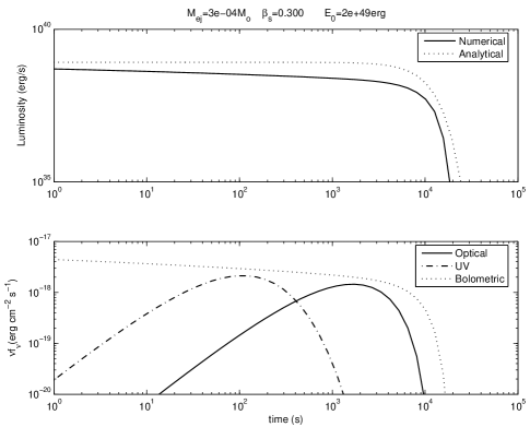
Figure 1: (Top) The luminosity, $L(t)$, for an explosion with no heating source. The model parameters ($M_{\rm ej}$ and $\beta_{s}$) are indicated on the title line. The thick line is obtained from numerical integration (Equation 5) whereas the dotted line is the (photon dominated) analytical formula (Equation 8). The numerical curve tracks the analytical curve (apart from a scaling of 0.6); the two disagree as the MN evolves (see text). (Bottom) The optical and UV broad-band fluxes ($\nu f_{\nu}$) expected for a macronova located at a redshift of $z=0.2$. The dotted line is the bolometric flux, $L(t)/(4\pi D^{2})$ where $D=0.97\,$Gpc is the distance.

The analytical formula allow us to get some insight into the overall behavior of the luminosity evolution. First, we note that $t_{h}=R_{0}/v_{s}=0.3\beta_{s}^{-1}\,$ms is much smaller than $t_{d}(0)=6.2\times 10^{3}(M_{\rm ej}/10^{-3}\,M_{\odot})\,$yr. The internal energy, $E$, decreases on the initial hydrodynamical scale and immediately justifies our coasting approximation. Next, the duration of the signal is given by the geometric mean of $t_{d}(0)$ and $t_{h}$ and is $\propto(M_{\rm ej}/v_{s})^{1/2}$ but independent of $R_{0}$. The duration is not all that short, $\sim 0.3(M_{\rm ej}/10^{-3}\,M_{\odot})^{1/2}(\beta_{s}/0.1)^{-1/2}\,d$. Third, the peak emission, $E_{0}/t_{d}(0)=\beta_{s}^{2}c^{3}R_{0}/(2B\kappa)$, is independent of the mass of the ejecta but directly proportional to $R_{0}$ and the square of the final coasting speed, $v_{s}^{2}$.

Unfortunately, as can be seen from Figure 1 (bottom panel), model light curves for a macronova located at $z=0.2$ is beyond current capabilities in any band even in the best case (high $\beta_{s}$). This pessimistic conclusion is a direct result of small $R_{0}$, small $M_{\rm ej}$ and great distance ($\sim 1\,$Gpc) for short hard bursts.

The situation is worse for lower shock speeds. A lower shock speed means a lower photon temperature and thus lower photon pressure. The luminosity decreases by an additional factor $\propto(t/t_{h})^{-1}$ (Equation 9). Next, the internal energy is shared equitably between photons and particles and a lower photon density means that a larger fraction of the internal energy is taken up the particles. Indeed, one can see a hint of the latter process in Figure 1 where the numerical curve (proceeding from start of the burst to later times) is increasingly smaller than the analytical curve. This is entirely a result of equipartition of $E$ between photons and particles and this equipartition is not accounted for by in deriving Equation 8.

4 Heating by Neutron Decay

On a timescale (half lifetime) of 10.4 minutes, a free neutron undergoes beta decay yielding a proton, a mildly relativistic electron with mean energy, 0.3 MeV) and an antineutrino. Thus the heating rate is entirely due to the newly minted electron (see Appendix) and is

$$\varepsilon_{n}(t)=3.2\times 10^{14}\,\mathrm{erg\,g^{-1}\,s^{-1}}.$$ (10)

Even though there are two unconstrained model physical parameters, $M_{\rm ej}$ and $\beta_{s}$, a constraint may be reasonably imposed by the prejudice that the macronova energy is, at best, comparable to the gamma-ray energy release which we take to be $10^{49}\,$erg (Fox et al., 2005). Within this overall constraint I consider two extreme cases for the neutron ejecta model: a high velocity case, $\beta_{s}=0.3$ and a low(est) velocity case, $\beta_{s}=0.05$. The mass of the ejecta was chosen so that $E_{0}\sim 10^{49}\,$erg. The range in $\beta$ is nicely bracketed by these two cases. The escape velocity of a neutron star is $0.3c$. The energy released per neutron decay of 0.3 MeV is equivalent to $\beta_{s}=0.025$. Clearly, final ejecta speeds below this value seem implausible (even such a low value is implausible especially when considering that the ejecta must first escape from the deep clutches of a compact object). By coincidence, as discussed below, these two cases nicely correspond to a photon dominated and gas pressure dominated case, respectively.

  

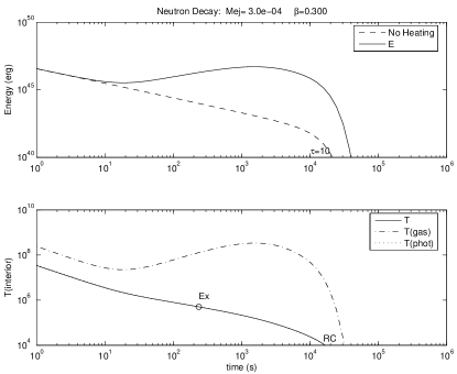
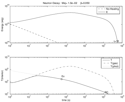
Figure 2: (Top) Internal energy ($E$) with (solid line) and without (dashed line) neutron decay heating. (Bottom) The interior temperature obtained by solving Equation 1 (solid line) given $E$ and radius, $R$. The dash-dotted line is the temperature one would obtain if all the internal energy was in particles whereas the dotted line is that obtained if the photons dominated the internal energy. Each vertical pair of panels refers to a choice of model parameters: coasting speeds of $\beta_{s}=0.3$ (left) and $\beta_{s}=0.05$ (right). The explosion energy, $E_{0}=1/2v_{s}^{2}M_{\rm ej}\sim 2\times 10^{49}\,$erg in both cases. “RC” marks the epoch at which the surface temperature falls below $T_{c}=10^{4}\,$K and $\tau=10$ marks the epoch at which electron scattering optical depth is 10. “Ex” marks the epoch at which all the initial photons are radiated away.

The decay of neutrons extends the hot phase of the fireball expansion (Figure 2). This is nicely demonstrated in Figure 2 (right set of panels) where we see that the decay of neutrons reverses the decrease in the internal energy. Indeed for the $\beta_{s}=0.05$ case neutron heating results in the pressure switching from being dominated by gas to a photon dominated ejecta. It is this gradual heating that makes a neutron MN potentially detectable.

I now carry out a number of self-consistency checks. To start with, implicit in Equations 1 and 3 is the assumption that the ions, electrons and photons have the same temperature. From the Appendix we see that the electron-electron and electron-ion timescales are very short and we can safely assume that the electrons and ions are in thermal equilibrium with respect to each other.

Next, I consider the time for the electrons to equilibrate with the photons. There are two parts to this issue. First, the slowing down of the ejected beta particle (electron). Second, the equilibration of thermal electrons with photons. The energetic electron can be slowed down by interaction with thermal electrons and also by interaction with photons. In the Appendix we show that the slowing down and thermalization timescales have essentially the same value:

$$t(\gamma,e)=\frac{3}{4}\frac{m_{e}c}{\sigma_{T}aT^{4}}=\Bigg{(}\frac{T}{2.7\times 10^{5}\,\mathrm{K}}\Bigg{)}^{-4}\,\mathrm{s}.$$ (11)

Thus when the interior temperature falls below (say) $2.7\times 10^{4}\,$K the photon-electron equilibration time becomes significant, about $10^{4}\,$s. (However, by this time, most of the neutrons would have decayed and all that realistically matters is the photon-matter thermalization timescale).

An entirely independent concern is the availability of photons for radiation at the surface. At the start of the explosion, by assumption, all the internal energy, $E_{0}$, is in photons and thus the initial number of photons is $N_{\mathrm{ph}}(0)=E_{0}/(2.7k_{B}T_{0})$ where $E_{0}=V_{0}aT_{0}^{4}$, $V_{0}=4\pi/3R_{0}^{3}$ is the initial volume and $a$ is the Stefan-Boltzmann radiation constant (see Appendix). Photons are continually lost at the surface. Electron scattering does not change the number of photons. Thus an important self-consistency check is whether the number of radiated photons is consistent with the number of initial photons. However, as can be seen from Figure 2 the number of radiated photons exceeds the number of initial photons in less than ten minutes after the explosion (the epoch is marked “Ex”). Relative to the observations with large ground based telescopes this is a short timescale and so it is imperative that we consider the generation of new photons.

4.1 Free-free emission as a source of new photons

For a hot plasma with $A=Z=1$, the free-free process is the dominant source of photon creation. The free-free process is flat, $f_{\nu}\propto\exp(-h\nu/k_{B}T)$ whereas the blackbody spectrum exhibits the well known Planck spectrum. Thus the free-free process will first start to populate the low-frequency end of the spectrum. Once the energy density, at a given frequency, reaches the energy density of the black body spectrum at the same frequency, then free-free absorption will suppress further production of free-free photons.

  

Figure 3: Photon diffusion ($t_{\mathrm{d}}$) timescale and photon-electron equilibration ($t_{e^{,}\mathrm{\gamma}}$) timescales, relative to the expansion time ($t$), as a function of $t$. The epoch at which these timescales match the expansion time are marked by an open square or open circle.

  

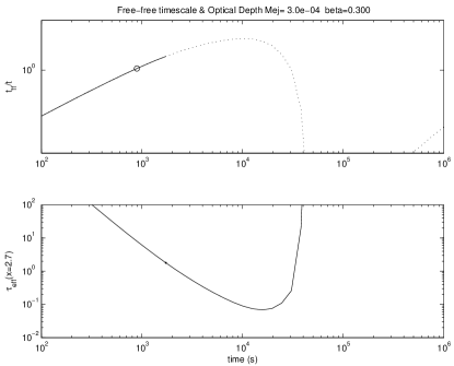
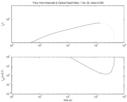
Figure 4: Run of the free-free timescale, $t_{\mathrm{ff}}$ (top panel) and the effective free-free optical depth ($\tau_{*}$) evaluated at normalized frequency $x=h\nu/k_{B}T=2.7$ (bottom panel). The timescales are normalized by time past the explosion. The free-free timescale is only meaningful when the effective optical depth is above unity (we have chosen $\tau_{*}=2$ as the criterion) and the range of epochs for which this is the case is marked by a solid line. The epoch at which free-free emission is unable to keep the interior stocked with the blackbody photon density is marked by an open square (top panel). Right. The curves are for $\beta_{s}=0.05$ and $M_{\rm ej}=10^{-2}\,M_{\odot}$. The macronova never gets optically thin and hence the absence of squares. Left. The curves are for $\beta_{s}=0.3$ and $M_{\rm ej}=3\times 10^{-4}\,M_{\odot}$. Seemingly $t_{d}$ rises at late times but this artifact is of little consequence since there is no emission beyond $10^{4}\,$s.

Provided the free-free optical depth, $\tau_{\mathrm{ff}}(\nu)=R\alpha_{\mathrm{ff}}(\nu)$ (Appendix) is $\mathrel{\hbox{\hbox to0.0pt{\hbox{\lower 4.0pt\hbox{$\sim$}}\hss}\hbox{$>$}}}1$ for $\nu\mathrel{\hbox{\hbox to0.0pt{\hbox{\lower 4.0pt\hbox{$\sim$}}\hss}\hbox{$>$}}}kT/h$ a simple estimate for the timescale over which the free-free process can build a photon density equal to that of the black body radiation field (of the same temperature) is given by

$$t_{\mathrm{ff}}=\frac{aT^{4}}{\epsilon_{\mathrm{ff}}(n_{e},n_{i},T)};$$ (12)

here, $\epsilon_{\mathrm{ff}}(n_{e},n_{i},T)$ is the frequency integrated free-free volume emissivity (see Appendix). However, electron scattering increases the effective optical depth of the free-free process (Rybicki & Lightman 1979, p. 33)

$$\tau_{*}(\nu)=\sqrt{\tau_{\mathrm{ff}}(\nu)(\tau_{\mathrm{ff}}(\nu)+\tau_{\mathrm{es}})}\ .$$ (13)

$\tau_{*}$ takes into account that the relevant optical depth for any emission process is the distance between the creation of a photon and the absorption of the photon. Electron scattering increases the probability of a newly minted photon to stay within the interior and thereby increases the free-free optical depth.

Even after free-free process stops producing photons, the photons in the interior are radiated on the photon diffusion timescale (Equation 6). These two processes, the increase in the effective optical depth and the photon diffusion timescale, prolong the timescale of the macronova signal, making the macronova signal detectable by the largest ground-based optical telescopes (which unlike robotic telescopes respond on timescales of hours or worse).

In Figures 3 and 4, I present various timescales ($t_{\rm d}$, $t_{\gamma,e}$, $t_{\mathrm{ff}}$) and the frequency at which the effective free-free optical depth (Equation 13) is unity. For $\beta_{s}=0.05$, $t_{\mathrm{ff}}$ is always smaller than $t$ and this means that the free-free process keeps the interior well stocked with photons. The remaining timescales are longer, approaching a day.

For $\beta_{s}=0.3$ we find that $\tau_{*}$ as evaluated at $x=h\nu/k_{B}T=2.7$ falls below 2 at about 2,000 s. Thus, for epochs smaller than 2,000 s we can legitimately evaluate $t_{\mathrm{ff}}$. We find that $t_{\mathrm{ff}}$ exceeds $t$ at about 1,000 s (marked by “ff”). We consider this epoch to mark the epoch at which free-free emission “freezes” out in the sense that there is no significant production of free-free emission beyond this epoch. However, the photons in the interior leak out on the diffusion timescale which becomes comparable to the expansion time at $t\sim 10^{4}\,$s. In summary, there is no shortage of photons for surface radiation for ejecta velocity as high as $\beta_{s}=0.3$ but only for epochs earlier than $10^{4}\,$s.

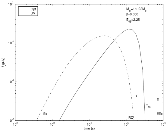
Figure 5: Optical and UV light curves for a macronova located at a redshift, $z=0.2$. The physical parameters, $M_{\rm ej}$ and $\beta$ are displayed in the Figure. The symbols at the bottom of the figure are as follows: “Ex” (exhaustion of initial photons), “ff” (epoch beyond which free-free emission can no longer keep the photon energy density at the black body energy density), “$\gamma$” (epoch at which electrons and photons decouple), “$\tau_{\rm es}$” (the electron scattering optical depth is 10 at this epoch), “RC” (the epoch at which the surface effective temperature is $10^{4}\,$K) and “ffEx” is the epoch at which all the free-free photons generated at the epoch marked “ff” are exhausted by radiation from the surface. In all cases the epoch is the left most character. Symbols appearing close to either left or right vertical axis may have been shifted to keep the symbols within the figure boundary.

4.2 The Light Curves

The expected light curves for a macronova at $z=0.2$ are shown in Figures 5 and 6. For $\beta=0.05$ the earliest constraining timescale is “RC” or the epoch marking the recombination of the electrons with ions. Beyond day one, the model presented here should not be trusted. For $\beta=0.3$, as discussed earlier and graphically summarized in Figure 6, the constraints come from photon production. Complete photon exhaustion takes place at the start of epoch of transparency (marked by “$\tau_{\rm es}$”) and so emission will cease rapidly at $10^{4}\,$s. Observations, if they have to any value, must be obtained within an hour or two.

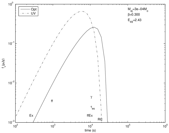
Figure 6: Expected light curve for a neutron decay powered macronova with $\beta_{s}=0.3$. The explanations of the symbols can be found in the caption to Figure 5.

The peak flux in Figures 5 and 6 is about $0.3\,\mu$Jy. With 15 minutes of integration time on a 10-m telescope one can easily detect this peak flux

Thus observations are capable of constraining a neutron powered MN with explosion energy comparable to $10^{49}\,$erg (the typical isotropic $\gamma$-ray energy release for short hard bursts). However, these observations have to be obtained on timescales of hours ($\beta_{s}=0.3$) to about a day ($\beta_{s}=0.05$).

Observations become less constraining with ejecta speeds larger than that considered here because the macronova becomes transparent earlier ($t\propto\beta_{s}^{-4}$, assuming that the explosion energy is constant) and as a result photons are lost on a timescale approaching the light crossing timescale i.e. rapid loss.

A potentially significant and non-trivial complication is confusion of the macronova signal by the afterglow emission. Optical afterglow emission has been seen for GRB 050709 (Hjorth et al., 2005) and GRB 050724 (Berger et al., 2005). Afterglow emission could, in principle, be disentangled from the macronova signal by obtaining multi-band data. Of particular value are simultaneous observations in the X-ray band. No X-ray emission is expected in the macronova model. Thus, X-ray emission is an excellent tracer of the afterglow emission. An alternative source for X-rays is some sort of a central long-lived source. As discussed in §6 a macronova would reprocess the X-ray emission to lower energies. Thus, the X-ray emission, at least in the macronova model, is a unique tracer of genuine afterglow emission and as a result can be used to distinguish a genuine macronova signal from ordinary afterglow emission.

5 Heating by Nickel

In the previous section I addressed in some detail photon generation and photon-matter equilibration for $A=Z=1$ plasma. Here, I present light curves with Nickel ejecta. The many transitions offered by Nickel ($Z=28$, $A=56$) should make equilibration less of an issue. Next, free-free mechanism becomes increasingly more productive for higher $Z$ ions ($\propto Z^{2}$; see Appendix). Thus the time for free-free photons to be exhausted, a critical timescale should be longer a Nickel MN (for a given $M_{\rm ej}$ and $\beta$) relative to a neutron MN.

There is one matter that is important for a Nickel MN and that is the issue of heating of matter. In a Nickel MN matter is heated by deposition of gamma-rays released when Nickel decays to Cobalt. Relative to the SN case, the energy deposition issue is important for an MN both because of a smaller mass of ejecta and also higher expansion speeds.

The details of Nickel $\rightarrow$ Cobalt $\rightarrow$ Iron decay chain and the heating function are summarized in the Appendix. In view of the fact that most of our constraints come from early time observations (less than 10 days) we will ignore heating from the decay of Cobalt. Thus

$$\varepsilon_{\rm Ni}(t)=3.9\times 10^{10}f_{\rm Ni}\exp(-\lambda_{\rm Ni}t)\,{\rm erg\,g^{-1}s^{-1}},$$ (14)

where $\lambda_{\rm Ni}^{-1}=8.8\,$d and $f_{\rm Ni}$ is the mass fraction of radioactive Nickel in the ejecta and is set to 1/3.

Nickel decay results in production of $\gamma$-rays with energies between 0.158 and 1.56 MeV (see Appendix). Colgate et al. (1980) find that the $\gamma$-ray mass absorption opacity is 0.029 cm² g^-1 for either the Ni⁵⁶ or Co⁵⁶ $\gamma$-ray decay spectrum. Extraction of energy from the gamma-rays requires many scatterings (especially for the sub-MeV gamma-rays) and this “deposition” function was first computed by Colgate et al. (1980). However, the $\varepsilon(t)$ we need in Equation 2 is the deposition function averaged over the entire mass of the ejecta. To this end, using the local deposition function of Colgate et al. (1980), I calculated the bulk deposition fraction, $\eta_{\mathrm{es}}$ (for a uniform density sphere) and expressed as a function of $\tau_{\rm es}$, the center-to-surface Thompson optical depth. The net effective heating rate is thus $\eta_{\mathrm{es}}\varepsilon_{\rm Ni}(t)$. I find that only 20% of the $\gamma$-ray energy is thermalized for $\tau_{\rm es}=10$. Even for $\tau_{es}=100$ the net effective rate is only 70% (because, by construction, the ejecta is assumed to be a homogeneous sphere; most of the $\gamma$-rays that are emitted in the outer layers escape to the surface).

The resulting lightcurves are plotted in Figure 7 for $\beta_{s}=0.03$ and $\beta_{s}=0.3$. I do not compute the UV light curve given the high opacity of metals to the UV. As with Ia supernovae, peak optical emission is achieved when radioactive power is fully converted to surface radiation (Arnett, 1979; Chevalier, 1981).

$\beta_{s}=0.03$ is a sensible lower limit for the ejecta speed; equating the energy released by radioactive decay to kinetic energy yields $\beta_{s}=0.01$. Peak optical emission is achieved at day 5. At this epoch, the photospheric temperature is in the vicinity of $T_{\rm RC}=5\times 10^{3}\,$K. Thus the calculation should be reasonably correct up to this epoch. Extrapolating from the neutron MN case for similar model parameters I find that photon production and equilibration are not significant issues.

For $\beta_{s}=0.3$, peak emission occurs at less than a day, again closely coincident with the epoch when the effective photospheric temperature is equal to $T_{\rm RC}$. For the neutron MN the exhaustion of the free-free photons was the limiting timescale ($\sim 10^{4}\,$s). Qualitatively this timescale is expected to scale as $Z$ (§5) and if so the model light curve up to the peak value is reliable.

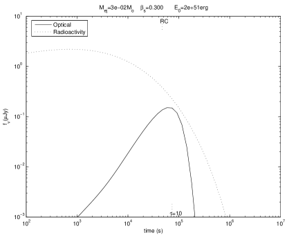
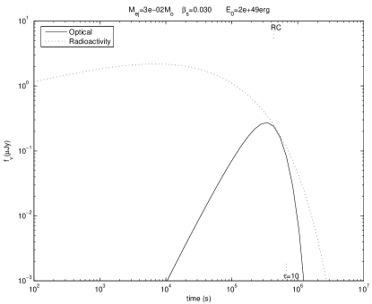
Figure 7: Model light curve for a macronova at $z=0.22$ and powered by radioactive Nickel (one third by mass). The dotted line is the expected light curve if Nickel radioactive decay power is instantly converted to the optical band. The input includes only the fraction of $\gamma$-rays that are absorbed and thermalized within the ejecta (i.e. $\varepsilon_{\rm Ni}(t)\eta_{\rm es}$). The slight curvature in the dotted line (between $10^{2}\,$s and $10^{4}\,$s) is an artifact of the least squares fit to the net energy deposition function (Equation 52). “RC” is the epoch at which the effective surface temperature is 5,000 K and the epoch at which the electron optical depth is 10 is marked.

To conclude, a Nickel powered MN is detectable only if the explosion speed is unreasonably low, $\beta_{s}=0.03$. Observations will not place significant constraints for $\beta_{s}=0.3$. For such rapid expansion, the MN suffers from lower deposition efficiency and an onset of transparency before the bulk of Cobalt has decayed. Conversely, there exists an opportunity for (futuristic) hard X-ray missions to directly detect the gamma-ray lines following a short hard burst!

6 The MN as a reprocessor

The simplest idea for short hard bursts is a catastrophic explosion with an engine that lives for a fraction of a second. However, we need to keep an open mind about the possibility that the event may not necessarily be catastrophic (e.g. formation of a millisecond magnetar) or that the engine or the accretion disk may live for a time scale well beyond a fraction of a second.

It appears that the X-ray data for GRB 050709 are already suggestive of a long lived source. A strong flare flare lasting 0.1 d and radiating $10^{45}\,$erg energy (and argued not to arise in the afterglow and hence by elimination to arise from a central source) is seen sixteen days after the event (Fox et al., 2005). The existence of such a flare in the X-ray band limits the Thompson scattering depth to be less than unity at this epoch. As can be seen from Figures 5 and 6 this argument provides a (not-so interesting) lower limit to the ejecta speed.

The main value of a macronova comes from the reprocessing of any emission from a long-lived central source into longer wavelengths. In effect, late time optical observations can potentially constrain the heating term in Equation 2, regardless of whether the heating arises from radioactivity or a long-lived X-ray source. In this case, $\varepsilon(t)M_{\mathrm{ej}}$ refers to the luminosity of the central source. The optical band is the favored band for the detection of such reprocessed emission (given the current sensitivity of facilities).

A central magnetar is a specific example of a long lived central source. The spin down power of an orthogonal rotator is

$$\varepsilon(t)=-\frac{B^{2}R_{n}^{6}\omega^{4}}{6c^{3}}$$ (15)

where $B$ is the dipole field strength, $R_{n}$ is the radius of the neutron, $\omega=2\pi/P$ is the rotation angular frequency and $P$ is the rotation period. For $B=10^{15}\,$G, $R_{n}=16\,$km we obtain $dE/dt\sim 10^{42}(P/100\,{\mathrm{ms}})^{-4}\,$erg s^-1 and the characteristic age is $5\times 10^{4}\,$s. Constraining such a beast (or something similar) is within the reach of current facilities (Figure 8).

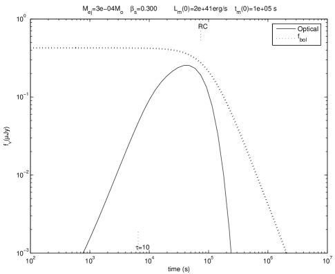
Figure 8: Expected optical light curve from a power law central source with $L_{m}(t)=L_{m}(0)(1+t/t_{m}(0)^{2})^{-1}$ with $L_{m}(0)=2\times 10^{41}\,$ erg s^-1 and $t_{m}(0)=10^{5}\,$s. The dotted line is the expected flux if the power from the central source is instantly and fully converted to the optical band. “RC” and “$\tau=10$” have the same meanings as in previous figures.

The power law decay discussed in this section is also applicable for neutron rich ejecta. For such ejecta arguments have been advanced that the resulting radioactive heating (from a variety of isotopes) can be approximated as a power law (see Li & Paczyński (1998)).

Earlier we discussed of the potential confusion between a macronova and afterglow emission. One clear distinction is that afterglow emission does not suffer from an exponential cutoff whereas a macronova dies down exponentially (when the optical depth decreases). However, quality measurements are needed to distinguish power law light curves of afterglow (flux $\propto t^{\alpha}$ with $\alpha=-1$ to $-2$) versus the late time exponential cutoff of macronova emission.

7 Conclusions

The prevailing opinion is that short duration bursts arise from the coalescence of a neutron star with another neutron star or a black hole. The burst of $\gamma$-rays requires highly relativistic ejecta. The issue that is very open is whether the bursts are also accompanied by a sub-relativistic explosion. This expectation is motivated from numerical simulations of coalescence as well as the finding of supernovae accompanying long duration bursts. Li & Paczyński (1998) were the first ones to consider the detection of optical signal from sub-relativistic explosions. Rather than referring to any such accompanying nova-like explosion as a “mini-supernova” (a term which only an astronomer will fail to recognize as an oxymoron) I use the term macronova (and abbreviated as MN).

Essentially a macronova is similar to a supernova but with smaller mass of ejecta. However, there are important differences. First, supernova expand at relatively slow speed, $\sim 10^{9}\,$cm s^-1 (thanks to the smalle escape velocity of a white dwarf). Next, radioactivity, specifically the decay of radioactive Nickel plays a key role in powering supernovae. The large mass of the ejecta, the slow expansion and the 9-day and 111-day $e$-folding timescale of Nickel and Cobalt (resulting in a gradual release of radioactive energy) all conspire to make supernovae attain significant brightness on a timescale well suited to observations, namely weeks.

A macronova has none of these advantages. On general grounds, the mass of ejecta is expected to be small, $10^{-2}\,M_{\odot}$. The expansion speed is expected to be comparable to the escape velocity of a neutron star, $0.3c$. Finally, there is no reason to believe that the ejecta contains radioactive elements that decay on timescales of days.

In this paper, I model the optical light curve for a macronova powered by decaying neutrons or by decay of radioactive Nickel. The smaller mass and the expected higher expansion velocities necessitate careful attention to various timescales (photon generation, photon-matter equilibrium, gamma-ray energy deposition).

Surprisingly a neutron powered MN (with reasonable explosion parameters) is within reach of current facilities. Disappointingly a Nickel powered MN (with reasonably fast expansion speed) require deeper observations to provide reasonable constraints. This result is understandable in that a MN is not only a smaller supernova but also a speeded up supernova. Thus the detectability of a MN is intimately connected with the decay time of radioactive elements in the ejecta. Too short a decay (seconds) or too long a decay (weeks) will not result in a bright signal. For example, artificially changing the neutron decay time to 90 s (whilst keeping the energy released to be the same as neutron decay) significantly reduces the signal from a macronova so as to (effectively) render it undetectable. The difficulty of detecting Nickel powered MN illustrate the problem with long decay timescales.

Next, I point out that a central source which lives beyond the duration of the gamma-ray burst acts in much the same way as radioactive heating.

Finally, it is widely advertised that gravitational wave interferometers will provide the ultimate view of the collapse which drive short hard bursts. However, these interferometers (with appropriate sensitivity) are in the distant future. Rapid response with large telescopes has the potential to directly observe the debris of these collapses – and these observations can be done with currently available facilities. This scientific prize is the strongest motivation to mount ambitious campagins to detect and study macronovae.

To date, GRB 050509b was observed rapidly (timescales of hours to days) with the most sensitive facilities (Keck, Subaru and HST). The model developed here has been applied to these data and the results reported elsewhere.

Appendix: Formulae & Approximations used in the paper

Blackbody Radiation

The blackbody spectral intensity is

$$B_{\nu}(T)=\frac{2}{\lambda^{2}}\frac{h\nu}{\exp({-h\nu/kT})-1}\,\,\mathrm{erg\,cm}^{-2}\,\mathrm{s}^{-1}\,\mathrm{ster}^{-1}\,\mathrm{Hz}^{-1}.$$ (16)

Frequently it helps to use physically normalized frequency unit, $x=h\nu/(k_{B}T)$. Then,

$$B_{x}(T)=\frac{2h}{c^{2}}\Big{(}\frac{kT}{h}\Big{)}^{4}\frac{x^{3}}{\exp(x)-1}.$$ (17)

The spectral energy density is

$$u_{\nu}(T)=\frac{4\pi}{c}B_{\nu}(T).$$

The photon number density is

$$n(<\nu) = \int_{0}^{\nu}\frac{4\pi}{c}\frac{B_{\nu}(T)}{h\nu}d\nu$$ (18)

$$n(<x) = 8\pi\Big{(}\frac{kT}{h}\Big{)}^{3}\int_{0}^{x}\frac{x^{2}}{\exp(x)-1}dx$$ (19)

$$= 8\pi\Big{(}\frac{kT}{hc}\Big{)}^{3}\Gamma(3)\zeta_{3}(x)$$ (20)

$$= 16\pi\Big{(}\frac{kT}{hc}\Big{)}^{3}\zeta_{3}(x);$$ (21)

where $\zeta_{n}(x)\equiv\Gamma(n)^{-1}\int_{0}^{x}t^{n-1}/(e^{t}-1)dt$ is an incomplete $\zeta$ function of order $n$. We note that $\zeta_{3}(\infty)=1.202$ and $\zeta_{4}(\infty)=\pi^{4}/90$. Thus the number of photons per unit volume is $n_{0}=19.2\pi(kT/hc)^{3}$. The mean energy of the photon defined as $u(T)/n_{0}$ is $2.7kT$. In the Rayleigh-Jeans approximation, we obtain

$$n(<x)=16\pi\Big{(}\frac{kT}{hc}\Big{)}^{3}\frac{x^{2}}{4}$$ (22)

This equation demonstrates that most of the photons have $x>1$ (with less than 20% of photons with $x<1$). The fiftieth percentile is $x=2.36$.

Free-free Emission

The free-free volume emissivity rate (Rybicki & Lightman 1979, p. 160) is

$$\epsilon_{\mathrm{ff}}(\nu)=6.8\times 10^{-38}Z^{2}n_{e}n_{i}T^{-1/2}\exp(-h\nu/k_{B}T)\bar{g}_{\mathrm{ff}}\,\,\mathrm{erg}\,\mathrm{cm}^{-3}\mathrm{s}^{-1}\mathrm{Hz}^{-1}.$$ (23)

Here, $\bar{g}_{\mathrm{ff}}$ is the velocity-averaged Gaunt factor and varies from 5 to 1 as $u=h\nu/k_{B}T$ ranges from $10^{-4}$ to 1. It appears to me that $\bar{g}_{\mathrm{ff}}=-\log(u)+1$ provides a reasonable approximation (for $u<1$). The frequency integrated emissivity ($Z=A=1$)

$$\epsilon_{\mathrm{ff}}=1.4\times 10^{-27}n_{e}^{2}T^{1/2}\bar{g}_{B}\,\,\mathrm{erg\,cm}^{-3}\,\mathrm{s}^{-1}$$ (24)

where $\bar{g}_{B}$ is the frequency-averaged Gaunt factor and a value of 1.2 gives 20% accuracy. For very hot plasma, relativistic effects become important and the rate increases by a factor of $1+T/2.2\times 10^{9}\,\mathrm{K}$.

The free-free density absorption coefficient, $\alpha_{\nu}(\mathrm{ff})$ $=n\sigma_{\nu}(\mathrm{ff})$ is given (it op cit., p. 162)

$$\alpha_{\nu}(\mathrm{ff})=3.7\times 10^{8}T^{-1/2}Z^{2}n_{e}n_{i}\nu^{-3}(1-\exp(-h\nu/k_{B}T))\,\mathrm{cm}^{-1}\bar{g}_{\mathrm{ff}}$$ (25)

As noted in the previous section, it is useful to work in normalized frequency units, $x=h\nu/kT$. Noting $\epsilon_{\mathrm{ff}}(x)=(kT/h)\epsilon_{\mathrm{ff}}(\nu)$ we find ($Z=A=1$)

$$\epsilon_{\mathrm{ff}}(x)=1.42\times 10^{-27}n^{2}T^{1/2}\exp(-x)\,\mathrm{erg\,cm}^{-3}\,\mathrm{s}^{-1}.$$ (26)

The number of photons above a value of $x$ is given by the integral $y(x)=\int_{x}^{\infty}t^{-1}\exp(-t)dt$. Though simple looking, this integral has no solution with known functions. The usual (sensible) approximation recognizes that there are few photons with $x>1$ and thus the upper limit can be replaced by unity. The next approximation is replace the exponential by unity. Thus $y(x)=-\log(x)$ (with implicit understanding $x<1$). Alternatively, an empirical function (obtained by numerical fitting),

$$y(x)=0.306-0.413\log(x)+0.094\log(x)^{2},$$ (27)

provides a reasonable fit for $10^{-2}<x<5$.

Photon-electron equilibration timescale

For a pure $A=Z=1$ gas, the primary primary photon-matter interaction for very hot gas is through Thompson scattering of electrons. Here we summarize the basic physics of the timescale of thermalizing a fast moving electron by the radiation field as well as the thermal photon-thermal electron equilibration timescale.

Consider the fate of the electron ejected as a result of neutron decay. The initial Lorentz factor of the electron ($\gamma_{0}$) can range from 3.5 to unity with a mean value of 1.6. The typical ejected electron is much hotter than the radiation field (temperature $T$) and will cool down by inverse scattering the ambient photons. The rate of energy loss is

$$\frac{dE}{dt}=-\frac{4}{3}\sigma_{T}c\gamma^{2}\beta_{s}^{2}U_{\rm ph}.$$ (28)

where the kinetic energy of the electron at any instant is given by $E=(\gamma-1)m_{e}c^{2}$. Simplifying I obtain

$$\frac{d\gamma}{dt}=A(1-\gamma^{2})$$ (29)

where $A={4\sigma_{T}cU_{\rm ph}}/{3m_{e}c^{2}}$. Since $\int dx(1-x^{2})^{-1}=(1/2)\log((x+1)/(x-1))$ we find that the electron loses a large fraction of energy over timescales of $A^{-1}$.

Next we consider an electron with energies comparable to that of photons. Consider an electron moving with velocity $v$ with respect to the radiation field. In the electron rest frame the radiation temperature is Doppler shifted as follows:

$$T(\theta)=T(1+v/c)\cos(\theta)$$ (30)

and correspondingly the total intensity also has an angular dependence given by

$$I(\theta)=\frac{ac}{4\pi}T(\theta)^{4}.$$ (31)

The momentum is $I(\theta)/c$ and the rate of momentum transfer to the electron is

$$F = -\int\sigma_{T}\frac{I(\theta)}{c}\cos(\theta)d\Omega$$ (32)

$$= -\frac{4}{3}\sigma_{T}aT^{4}\frac{v}{c}$$ (33)

Averaging the velocity over the thermal distribution, the work done by the radiation drag on the electron is

$$\langle-Fv\rangle = \frac{4}{3}\sigma_{T}T^{4}\langle\frac{v^{2}}{c}\rangle$$ (34)

$$= 4\sigma_{T}aT^{4}\frac{kT_{e}}{m_{e}c}$$ (35)

where we have made use of the well known formula $1/2m_{e}\langle v^{2}\rangle=3/2kT_{e}$. However, the electrons must be getting heated up by fluctuations in the radiation field because in equilibrium, when $T=T_{e}$, the electron will neither gain energy nor lose (on average). Thus the heat equation for the electron is

$$\frac{dQ}{dT}=4\sigma_{T}aT^{4}k(T-T_{e})/m_{e}c.$$ (36)

For fully ionized matter, $Q=3kT_{e}$ and thus we get the equation well known to cosmologists (Peebles, 1971)

$$\frac{dT_{e}}{dt}=-A(T_{e}-T)$$ (37)

where $U_{\rm ph}=aT^{4}$. The thermalization timescale is thus $\sim A^{-1}$.

Electron and Ion Equilibration

A fast electron will lose energy to slow moving electrons by Rutherford scattering. From Padmanabhan (2000, volume I, pp. 439) we see

$$t(e,e) = \frac{1}{4\pi}\frac{m_{e}^{1/2}(k_{B}T_{e})^{3/2}}{e^{4}nL_{e}}=10^{-2}T_{e,7}^{3/2}n_{11}^{-1}\,\mathrm{s},$$ (38)

$$t(i,i) = \frac{1}{4\pi}\frac{M^{1/2}(k_{B}T_{i})^{3/2}}{e^{4}nL_{i}}=4.3\times 10^{-1}T_{i,7}^{3/2}n_{11}^{-1}\,\mathrm{s},\ {\rm and}$$ (39)

$$t(e,i) = \Bigg{(}\frac{9\pi}{8}\Bigg{)}^{1/2}\frac{1}{Z^{2}}\Bigg{(}\frac{M}{m_{e}}\Bigg{)}t(e,e)=10Z^{-2}T_{e,7}^{3/2}n_{11}^{-1}\,\mathrm{s}.$$ (40)

Here $M$ is the mass of the ion and $L_{e}$ ($L_{i}$) refers to the usual logarithmic factor for electrons (ions) and set to 10. $n$ is the particle density (cm^-3) and the density normalization of $10^{11}\,$cm^-3 is appropriate for radius of $10^{14}\,$cm and ejecta mass of $M_{\rm ej}=10^{-3}\,M_{\odot}$.

Heating by Neutron Decay

A free neutron decays to a proton, electron and antineutrino. The half lifetime of the decay is 10.4 minutes and thus the $e$-folding time, $t_{N}=900\,$s. The mass difference between the neutron and that of the electron and proton is $Q=0.782$ MeV (see for example, Krane 1988).

The sum total linear momentum is conserved and the energy carried off by the electron and antineutrino must add up to $Q$. This would nominally suggest that there are five remaining free parameters ($3\times 3$ momenta minus four constraints). Thus the output of decay can now be described by five free parameters and we choose these to be the momentum of the electron, ${\mathbf{p}}$, and two momenta of the antineutrino, ${\mathbf{q}}$.

The proton, by the virtue of its mass, obtains very little energy in the process. Thue the energy of the antineutrino is $E_{\bar{\nu}}=Q-T$ where, following the convention in nuclear physics, $T=E-m_{e}c^{2}$ is the kinetic energy and $E^{2}=p^{2}c^{2}+m_{e}^{2}c^{4}$ (here $p=\sqrt{\mathbf{p}\cdot\mathbf{p}}$). The magnitude of the momentum of the antineutrino is $q=E_{\bar{\nu}}/c$ (since the antineutrino has very low, if any, mass)

There is no preferred direction for ${\mathbf{p}}$ and the phase space (per unit volume) for the electron momentum to lie between $p$ and $p+dp$ and the antineutrino momentum to lie between $q$ and $q+dq$ is

$$dn_{e}dn_{\bar{\nu}}=\frac{4\pi p^{2}}{h^{3}}dp\frac{4\pi q^{2}}{h^{3}}dq.$$ (41)

Our goal is to determine the distribution of the momentum of the electron. To this end we integrate $dn_{e}dn_{\bar{\nu}}$ over $q$ but subject to the constraint $qc=Q-T$ and find

$$dn_{e}(p)\propto p^{2}(Q-T)^{2}dp.$$ (42)

We transform this distribution to the differential energy distribution of the electron, $dn_{e}(E)/dE$, using the usual rule of transformations

$$\frac{dn_{e}(E)}{dE} = \frac{dn_{e}(p)}{dp}\frac{dp}{dE}$$ (43)

$$\propto Ep(Q-T)^{2}.$$ (44)

For the case of a decaying neutron, we use the probability distribution given by Equation 44 and find that the mean kinetic energy of the electron is $\langle T\rangle=0.59\,m_{e}c^{2}$. Thus the heating rate per gram is $N_{A}\langle T\rangle/t_{N}=3.2\times 10^{14}\,$erg g^-1 s^-1.

Heating by Decay of Radioactive Nickel

⁵⁶Ni is produced whenever nuclear reactions are allowed to proceed to statistical equilibrium. This isotope enjoys the distinction of being the most packed nucleon (highest binding energy per nucleon). However, the isotope is unstable and decays as follows: ⁵⁶Ni(6.01 d)$\rightarrow^{56}$Co(77 d)$\rightarrow^{56}$Fe. The half lifetimes are given in the parenthesis. The decay proceeds by electron capture of a K shell electron. Following this capture, a neutrino is emitted and the ⁵⁶Co is left in an excited state, 1.72 MeV above the ground state. A variety of decays are possible from this state to the ground state of ⁵⁶Co: 1.56 MeV, 0.812 MeV, 0.75 MeV, 0.48 MeV, 0.27 MeV and 0.158 MeV (see Arnett 1996, p. 426). Cobalt decays by electron capture (80%) resulting in a spectrum of $\gamma$-rays of mean energy of 3.5 MeV per decay and beta-emission (20%) with mean energy of 0.14 MeV per decay (see Colgate et al. (1980)). We set $\langle E_{\rm Co}\rangle=3.5+0.14=3.64\,$MeV.

Let $N_{0}=N_{\rm Ni}(t=0)$ be the initial number of Nickel nuclei. Let $N_{\rm Co}$ be the number of Cobalt nuclei; we have $N_{\rm Co}(t=0)=0$. The time evolution of Nickel and Cobalt is given by well known parent-daughter relations:

$$N_{\rm Ni}(t) = N_{0}\exp(-\lambda_{\rm Ni}t)\ {\rm and}$$ (45)

$$N_{\rm Co}(t) = N_{0}\frac{\lambda_{\rm Ni}}{\lambda_{\rm Ni}-\lambda_{\rm Co}}\Bigg{(}\exp(-\lambda_{\rm Co}t)-\exp(-\lambda_{\rm Ni}t)\Bigg{)}.$$ (46)

Here, $\lambda_{\rm Ni}=t_{\rm Ni}^{-1}$ and $\lambda_{\rm Co}=t_{\rm Co}^{-1}$ with $t_{\rm Ni}=6.1/\log(2)$ d and $t_{\rm Co}=77/\log(2)$ d. The heating rates (per gram) are obtained by letting $N_{0}=(56m_{H})^{-1}$ and are

$$\varepsilon_{\rm Ni}(t) = \lambda_{\rm Ni}\Delta E_{\rm Ni}N_{\rm Ni}(t)$$ (47)

$$= 3.9\times 10^{10}\exp(-\lambda_{\rm Ni}t)\,\,{\rm erg\,g^{-1}\,s^{-1}}$$ (48)

$$\varepsilon_{\rm Co}(t) = \lambda_{\rm Co}\langle E_{\rm Co}\rangle N_{\rm Co}(t)$$ (49)

$$= 7\times 10^{9}\Bigg{(}\exp(-\lambda_{\rm Co}t)-\exp(-\lambda_{\rm Ni}t)\Bigg{)}\,\,{\rm erg\,g^{-1}\,s^{-1}}.$$ (50)

From an inspection of the heating curve one finds that Cobalt decay competes with Nickel (assuming full energy absorption) by day 17. In the main text we note that early time ($\mathrel{\hbox{\hbox to0.0pt{\hbox{\lower 4.0pt\hbox{$\sim$}}\hss}\hbox{$<$}}}1$ week) observations result in the best constraint (or even a discovery). Given this we can safely ignore the heating provided by the decay of Cobalt.

The next issue is efficiency with which the $\gamma$-rays emitted during the course of the decay of Nickel can transfer energy to the surrounding matter. Colgate et al. (1980) consider the deposition of energy by $\gamma$-rays emanating from decay of Ni⁵⁶ and Co⁵⁶. They find that the mass opacity of the $\gamma$-ray absorption is about 0.029 cm${}^{2}\,$g^-1, for either Ni⁵⁶ or Co⁵⁶ decay spectrum. They used a Monte Carlo photon transport code and found that at least for a uniform sphere, $D$, the fraction of the $\gamma$-ray absorbed by the matter at a given radius depends only on $\gamma$-ray optical depth (to the surface), $\tau_{\gamma}$:

$$D(\tau_{\gamma})=G[1+2G(1-G)(1-0.75G)]$$ (51)

where $G=\tau_{\gamma}/(1.6+\tau_{\gamma})$.

I integrated the net deposition fraction for spheres with center-to-surface optical Thompson optical depth, $\tau_{\rm es}$ ranging from 1 to $10^{17}$. A polynomial fit yields

$$\log(\eta(\tau_{\rm es}))=-0.0003z^{4}+0.0108z^{3}-0.1486z^{2}+0.8134z-1.4360$$ (52)

where $z=\log(\tau_{\rm es})$; here $\log$ refers to logarithm to the base 10.

For example, when $\tau_{\rm es}=10$ I find $\eta_{\gamma}=0.2$ i.e. 80% of the $\gamma$-rays escape to the surface. Even for $\tau_{\rm es}=100$ I find $\eta_{\gamma}=0.7$ i.e. about 30% escape to the surface (mainly the outer layers).

References

- Arnett (1996) Arnett, D. 1996, Supernova and Nucleosynthesis (Princeton University Press)
- Arnett (1979) Arnett, W. D. 1979, Astrophys. J., 230, L37
- Berger et al. (2005) Berger, E., Price, P. A., Cenko, S. B., Gal-Yam, A., Soderberg, A. M., Kasliwal, M., Leonard, D. C., Cameron, P. B., Frail, D. A., Kulkarni, S. R., Murphy, D. C., Krzeminski, W., Piran, T., Lee, B. L., Roth, K. C., Moon, D.-S., Fox, D. B., Harrison, F. A., Persson, S. E., Schmidt, B. P., Penprase, B. E., Rich, J., Peterson, B. A., & Cowie, L. L. 2005, ArXiv.org, 1, nature (in press)
- Bloom et al. (2005) Bloom, J. S., Prochaska, J. X., Pooley, D., Blake, C. W., Foley, R. J., Jha, S., Ramirez-Ruiz, E., Granot, J., Filippenko, S., Sigurdsson, S., Barth, A. J., Chen, H.-W., Cooper, M. C., Falco, E. E., Gal, R. R., Gerke, B. F., Gladders, M. D., Greene, J. E., Hennanwi, J., Ho, L. C., Hurley, K., Koester, B. P., Li, W., Lubin, L., Newman, J., Perley, D. A., Squires, G. K., & Wood-Vasey, W. M. 2005, submitted to Astrophys. J.
- Chevalier (1981) Chevalier, R. A. 1981, Astrophys. J., 246, 267
- Colgate et al. (1980) Colgate, S. A., Petschek, A. G., & Kriese, J. T. 1980, Astrophys. J., 237, L81
- Covino et al. (2005) Covino, S., Antonelli, L. A., Romano, P., Palmer, D., Markwardt, C., Burrows, D., Gehrels, N., Barthelmy, S., Chester, M., Hunsberger, S., & Cummings, J. 2005, GCN Circular 3665
- Eichler et al. (1989) Eichler, D., Livio, M., Piran, T., & Schramm, D. N. 1989, Nature, 340, 126
- Fox et al. (2005) Fox, D. B., Frail, D. A., Price, P. A., Kulkarni, S. R., Berger, E., Piran, T., Soderberg, A. M., Cenko, S. B., Cameron, S. B., Gal-Yam, A., Kasliwal, M. M., Moon, D.-S., Harrison, F. A., Nakar, E., Schmidt, B. P., Penprase, B., Chevalier, R. A., Kumar, P., Roth, K., Watson, D., Lee, B. L., Shectman, S., Phillips, M. M., Roth, M., McCarthy, P. J., Rauch, M., Cowie, L., Peterson, B. A., Rich, J., Kawai, N., Aoki, K., Kosugi, G., Totani, T., Park, H.-S., MacFadyen, A., & Hurley, K. C. 2005, Nature, 437, 840
- Freiburghaus et al. (1999) Freiburghaus, C., Rosswog, S., & Thielemann, F.-K. 1999, Astrophys. J., 525, L121
- Gehrels et al. (2005) Gehrels, N., Sarazin, C. L., O’Brien, P. T., Zhang, B., Barbier, L., Barthelmy, S. D., Blustin, A., Burrows, D. N., Cannizzo, J., Cummings, J. R., , Goad, M., Holland, S. T., Hurkett, C. P., Kennea, J. A., Levan, A., Markwardt, C. B., Mason, K. O., Meszaros, P., Page, M., Palmer, D. M., Rol, E., Sakamoto, T., Willingale, R., Angellini, L., Beardmore, A., Boyd, P. T., Breeveld, A., Campana, S., Chester, M. M., Chincarini, G., Cominsky, L. R., Cusumano, G., de Pasquele, M., Fenimore, E. E., Giommi, P., Gronwall, C., Grupe, D., Hill, J. E., Hinshaw, D., Hjorth, J., Hullinger, D., Hurley, K. C., Klose, S., Kobayashi, S., Kouveliotou, C., Krimm, H. A., Mangano, V., Marshall, F. E., McGowan, R. N. K., Moretti, A., Mushotzky, R. F., Nakazawa, K., Norris, J. P., Nousek, J. A., Osborne, J. P., Page, K., Parsons, A. M., Patel, S., Perri, M., Poole, T., Romano, P., Roming, P. W. A., Rosen, S., Sato, G., Schady, P., Smale, A. P., Sollerman, J., Starling, R., Still, M., Suzuki, M., Tagliaferri, G., Takahashi, T., Tashiro, M., Tueller, J., Wells, A. A., White, N. E., & Wijers, R. A. M. J. 2005, Nature, 437, 851
- Goodman (1986) Goodman, J. 1986, Astrophys. J., 308, L47
- Hjorth et al. (2005) Hjorth, J., Watson, D., Fynbo, J. P. U., Price, P. A., Jensen, B. L., Jorgensen, U. G., Kubas, D., Gorosabel, J., Jakobsson, P., Sollerman, J., Pedersen, K., & Kouveliotou, C. 2005, Nature, 437, 859
- Janka & Ruffert (2002) Janka, H.-T. & Ruffert, M. 2002, in ASP Conf. Ser. 263: Stellar Collisions, Mergers and their Consequences, 333–+
- Krane (1988) Krane, K. S. 1988, Introductory Nuclear Physics (John Wiley and Sons)
- Li & Paczyński (1998) Li, L. & Paczyński, B. 1998, Astrophys. J., 507, L59
- Nakar et al. (2005) Nakar, E., Gal-Yam, A., Piran, T., & Fox, D. B. 2005, astro-ph/0502148
- Paczynski (1986) Paczynski, B. 1986, Astrophys. J., 308, L43
- Padmanabhan (2000) Padmanabhan, T. 2000, Theoretical Astrophysics (Cambridge University Press)
- Peebles (1971) Peebles, P. J. E. 1971, Physical Cosmology (Princeton University Press)
- Prochaska et al. (2005) Prochaska, J. X., Bloom, J. S., Chen, H. ., Foley, R. J., Perley, D. A., Ramirez-Ruiz, E., Granot, J., Lee, W. H., Pooley, D., Alatalo, K., & Hurley, K. 2005, ArXiv Astrophysics e-prints
- Rosswog (2005) Rosswog, S. 2005, ArXiv Astrophysics e-prints
- Rybicki & Lightman (1979) Rybicki, G. B. & Lightman, A. P. 1979, Radiative Processes in Astrophysics (John Wiley and Sons)
- Tanvir et al. (2005) Tanvir, N., Chapman, R., Levan, A., & Priddey, R. 2005, ArXiv Astrophysics e-prints
- Villasenor et al. (2005) Villasenor, J., Lamb, D. Q., Ricker, G. R., Atteia, J.-L., Kawai, N., Butler, N., Nakagawa, Y., Jernigan, J. G., Barraud, C., Boer, M., Crew, G. B., Dezalay, J.-P., Donaghy, T. Q., Doty, J., Fenimore, E. E., Galassi, M., Graziani, C., Hurley, K., Levine, A., Martel, F., Matsuoka, M., Monnelly, G., Morgan, E., Olive, J.-F., Prigozhin, G., Sakamoto, T., Shirasaki, Y., Suzuki, M., Tamagawa, T., Torii, K., Vanderspek, R., Woosley, S. E., Yoshida, A., Braga, J., Manchanda, R., Pizzichini, G., Takagishi, K., & Yamauchi, M. 2005, Nature, 437, 855