Beyond ideal MHD: towards a more realistic modeling of relativistic astrophysical plasmas

Abstract

Many astrophysical processes involving magnetic fields and quasi-stationary processes are well described when assuming the fluid as a perfect conductor. For these systems, the ideal-magnetohydrodynamics (MHD) description captures the dynamics effectively and a number of well-tested techniques exist for its numerical solution. Yet, there are several astrophysical processes involving magnetic fields which are highly dynamical and for which resistive effects can play an important role. The numerical modeling of such non-ideal MHD flows is significantly more challenging as the resistivity is expected to change of several orders of magnitude across the flow and the equations are then either of hyperbolic-parabolic nature or hyperbolic with stiff terms. We here present a novel approach for the solution of these relativistic resistive MHD equations exploiting the properties of implicit-explicit (IMEX) Runge Kutta methods. By examining a number of tests we illustrate the accuracy of our approach under a variety of conditions and highlight its robustness when compared with alternative methods, such as the Strang-splitting. Most importantly, we show that our approach allows one to treat, within a unified framework, both those regions of the flow which are fluid-pressure dominated (such as in the interior of compact objects) and those which are instead magnetic-pressure dominated (such as in their magnetospheres). In view of this, the approach presented here could find a number of applications and serve as a first step towards a more realistic modeling of relativistic astrophysical plasmas.

1 Introduction

A vast number of astronomical observations suggests that magnetic fields play a crucial role in the dynamics of many phenonema of relativistic astrophyics, either on stellar scales, such as for pulsars, magnetars, compact X-ray binaries, short and long/gamma-ray bursts (GRBs) and possibly for the collapse of massive stellar cores, but also on much larger scales, as it is the case for radio galaxies, quasars and active galactic nuclei (AGNs). A shared aspect in all these phenomena is that the plasma is essentially electrically neutral and the frequency of collisions is much larger than the inverse of the typical timescale of the system. The MHD approximation is then an excellent description of the global properties of these plasmas and has been employed with success over the several decades to describe the dynamics of such systems well in their nonlinear regimes. Another important common aspect in these systems is that their flows are characterized by large magnetic Reynolds numbers ${\cal R}_{\rm M}=LV/\lambda=4\pi\sigma LV/c^{2}$, where $L$ and $V$ are the typical sizes and velocities, respectively, while $\lambda$ is the magnetic diffusivity and $\sigma$ is the electrical conductivity. For a typical relativistic compact object, ${\cal R}_{\rm M}\gg 1$ and, under these conditions, the magnetic field is essentially advected with the flow, being continuosly distorted and possibly amplified, but also essentially not decaying. We note that these conditions are very different from those traditionally produced in the Earth’s laboratories, where ${\cal R}_{\rm M}\ll 1$, and the resistive diffusion represents an important feature of the magnetic-field evolution.

A particularly simple and yet useful limit of the MHD approximation is that of the “ideal-MHD” limit. This is mathematically defined as the limit in which the electrical resistivity $\eta\equiv 1/\sigma$ vanishes or, equivalently, by an infinite electrical conductivity. It is within this framework that many multi-dimensional numerical codes have been developed over the last decade to study a number of phenomena in relativistic astrophysics and in fully nonlinear regimes (Komissarov, 1999b; Koide et al., 1999; Komissarov, 2001; Koldoba et al., 2002; Gammie et al., 2003; Del Zanna et al., 2003; Anninos et al., 2005; Duez et al., 2005; Shibata & Sekiguchi, 2005; Neilsen et al., 2006; Anton et al., 2006; McKinney, 2006a; Mignone & Bodo, 2006; Noble et al., 2007; Giacomazzo & Rezzolla, 2007; Del Zanna et al., 2007; Farris et al., 2008). The ideal-MHD approximation is not only a convenient way of writing and solving the equations of relativistic MHD, but it is also an excellent approximation for any process that takes place over a dynamical timescale. In the case of an old and “cold” neutron star, for example, the electrical and thermal transport properties of the matter are mainly determined by the transport properties of the electrons, which are the most important carriers of charge and heat. At temperatures above the crystallization temperature of the ions, the electrical (and thermal) conductivities are governed by electron scattering off ions and an approximate expression for the electrical conductivity is given by (Lamb, 1991) $\sigma\approx 10^{24}\left({10^{9}\ \rm K}/{T}\right)^{2}\left({\rho}/{10^{14}\ {\rm g\ cm}^{-3}}\right)^{3/4}\ {\rm s}^{-1}$, where $T$ and $\rho$ are the stellar temperature and mass density. Even for a magnetic field that varies on a length-scale as small as $L\simeq 0.1R$, (where $R$ is the stellar radius) the magnetic diffusion timescale is $\tau_{\rm diff}={4\pi L^{2}\sigma}/{c^{2}}\approx 3\times 10^{6}{\rm yr}$.

Clearly, at these temperatures and densities, Ohmic diffusion will be neglible for any process taking place on a dynamical timescale for the star, i.e., $\lesssim{\rm few\ s}$, and thus the conductivity can be considered as essentially infinite. However, catastrophic events, such as the merger of two neutron stars, or of a neutron star with a black hole, can produce plasmas with regions at much larger temperatures (e.g., $T\sim 10^{11-13}\ {\rm K}$) and much lower densities (e.g., $\rho\sim 10^{8-10}\ {\rm gcm}^{-3})$. In such regimes, all the transport properties of the matter will be considerably modified and non-ideal effects, absent in perfect-fluid hydrodynamics (such as bulk viscosity) and ideal MHD (such as Ohmic diffusion on a much shorter timescale $\tau_{\rm diff}\sim 10^{3}{\rm s}$) will need to be taken into account. Similar conditions are likely not limited to binary mergers but, for instance, be present also behind processes leading to long GRBs, thus extending the range of phenomena for which resistive effects could be important. Note also that these non-ideal effects in hydrodynamics (MHD) are proportional not only to the viscosity (resistivity) of the plasma, but also to the second derivatives of the velocity (magnetic) fields. Hence, even in the presence of a small viscosity (resistivity), their contribution to the overall conservation of energy and momentum can be considerable if the velocity (magnetic) fields undergo very rapid spatial variations in the flow. A classical example of the importance of resistive MHD effects in plasmas with high but finite conductivities is offered by current sheets. These phenomena are often observed in the solar activity and are responsible for the reconnection of magnetic field lines and changes in the magnetic field topology. While these phenomena are behind the emission of large amounts of energy, they are strictly forbidden within the ideal-MHD limit due to magnetic flux conservation and so can not be studied employing this limit.

Besides having considerably smaller conductivities, low-density higly magnetized plasmas are present rather generically around magnetized objects, constituting what is referred to as the “magnetosphere”. In such regions magnetic stresses are much larger than magnetic pressure gradients and cannot be properly balanced; as a result, the magnetic fields have to adjust themselves so that the magnetic stresses vanish identically. This scenario is known as the force free regime (because the Lorentz force vanishes in this case) and while the equations governing it can be seen as the low-inertia limit of the ideal-MHD equations (Komissarov, 2002; McKinney, 2006b), the force-free limit is really distinct from the ideal-MHD one. This represents a considerable complication since it implies that it is usually not possible to decribe, within the same set of equations, both the interior of compact objects and their magnetospheres.

Theoretical work to derive a fully relativistic theory of non-ideal hydrodynamics and non-ideal MHD has been carried out by several authors in the past (Israel, 1976; Stewart, 1977; Carter, 1991; Lichnerowicz, 1967; Anile, 1989) and is particularly simple in the case of the resistive MHD description. The purpose of this work is indeed that of proposing the solution of the relativistic resistive MHD equations as an important step towards a more realistic modelling of astrophysical plasmas. There are a number of advantages behind such a choice. First, it allows one to use a single mathematical framework to describe both regions where the conductivity is large (as in the interior of compact objects) and small (as in magnetospheres), and even the vacuum regions outside the compact objects where the MHD equations trivially reduce to the Maxwell equations. Second, it makes it possible to account self-consistently for those resistive effects, such as current sheets, which are energetically important and could provide a substantial modification of the whole dynamics. Last but not least, the numerical solution of the resistive MHD equations provides the only way to control and distinguish the physical resistivity from the numerical one. The latter, which is inevitably present and proportional to truncation error, is also completely dependent on the specific details of the numerical algorithm employed and on the resolution used for the solution.

As noted already by several authors, the numerical solution of the ideal-MHD equations is considerably less challenging than that of the resistive MHD equations. In this latter case, in fact, the equations become mixed hyperbolic-parabolic in Newtonian physics or hyperbolic with stiff relaxation terms in special relativity. The presence of stiff terms is the natural consequence of the fact that the diffusive effects take place on timescales that are intrinsically larger than the dynamical one. Stated differently, in such equations the relaxation terms can dominate over the purely hyperbolic ones, posing severe constraints on the timestep for the evolution. While considerable work has already been made to introduce numerical techniques to achieve efficient implementations in either regime (Komissarov, 2004; Komissarov et al., 2007; Komissarov, 2007; Reynolds et al., 2006; Graves et al., 2008), the use of these techniques in fully three-dimensional simulations is still difficult and expensive.

In order to benefit from the many advantages discussed above in the use of the resistive MHD equations, we here present a novel approach for the solution of the relativistic resistive MHD equations exploiting the properties of implicit-explicit (IMEX) Runge Kutta methods. This approach represents a simple but effective solution to the problem of the vastly different timescales without sacrificing either simplicity in the implementation or the numerical efficiency. By examining a number of tests we illustrate the accuracy of our approach under a variety of conditions and demonstrate its robustness. In addition, we also compare it with the alternative method proposed by Komissarov (2007) for the solution of the same set of relativistic resistive MHD equations. This latter approach employs Strang-splitting techniques and the analytical integration of a reduced form of Ampere’s law. While it works well in a number of cases, it has revealed to be unstable when applied to discontinuous flows with large conductivities; such difficulties were not encountered when solving the same problem within the IMEX implementation.

Because our approach effectively treats within a unified framework both those regions of the flow which are fluid-pressure dominated and those which are instead magnetic-pressure dominated, it could find a number of applications and serve as a first step towards a more realistic modeling of relativistic astrophysical plasmas.

Our work is organized as follows. In Sect. 2 we present the system of equations describing a resistive magnetized fluid, while in Section 3 we discuss the problems related to the numerical evolution of this system of equations and the numerical approaches developed to solve them. In particular, we introduce the basic features of the IMEX Runge-Kutta schemes and recall their stability properties. In Sect 4 we instead explain in detail the implementation of the IMEX scheme to the resistive MHD equations. Finally, in Sect. 5 we present the numerical tests carried out either in one or two dimensions and that span several prescriptions for the conductivity. Section 5 is also dedicated to the comparison with the Strang-splitting technique. The conclusions and the perspectives for future improvements are presented in Sect. 6, while Appendix A reviews our space discretization of the equations.

Hereafter we will adopt Gaussian units such that $c=1$ and employ the summation convention on repeated indices. Roman indices $a,b,c,...$ are used to denote spacetime components (i.e., from $0$ to $3$), while $i,j,k,...$ are used to denote spatial ones; lastly, bold italics letters represent vectors, while bold letters represent tensors.

2 The resistive MHD description

An effective description of a fluid in the presence of electromagnetic fields can be made by considering three different sets of equations governing respectively the electromagnetic fields, the fluid variables and the coupling between the two. In particular, the electromagnetic part can be described via the Maxwell equations, while the conservation of energy and momentum can be used to express the evolution of the fluid variables. Finally, Ohm’s law, whose exact form depends on the microscopic properties of the fluid, expresses the coupling between the electromagnetic fields and the fluid variables. In what follows we review these three sets of equations separately, discuss how they then lead to the resistive MHD description, and how the latter reduces to the well-known limits of ideal-MHD and of the Maxwell equations in vacuum. Our presentation will be focussed on the special-relativistic regime, but the extension to general relativity is rather straightforward and will be presented elsewhere.

The Maxwell equations

The special relativistic Maxwell equations can be written as (Landau & Lifshitz, 1980)

$$\partial_{b}F^{ab} = I^{a}\,,$$ (1)

$$\partial_{b}^{~{}*}\!F^{ab} = 0\,,$$ (2)

where $F^{ab}$ and ${}^{~{}*}\!F^{ab}$ are the Maxwell and the Faraday tensor respectively and $I^{a}$ is the electric current 4-vector. A highly-ionized plasma has essentially zero electric and magnetic susceptibilities and the Faraday tensor is then simply the dual of the Maxwell tensor. This tensor provides information about the electric and magnetic fields measured by an observer moving along any timelike vector $n^{a}$, namely

$$F^{ab}=n^{a}E^{b}-n^{b}E^{a}+\epsilon^{abc}B_{c}\,.$$ (3)

We are considering $n^{a}$ to be the time-like traslational killing vector field in a flat (Minkowski) spacetime, so $n_{a}=(-1,0,0,0)$ and the Levi-Civita symbol $\epsilon^{abc}$ is non-zero only for spatial indices. Note that the electromagnetic fields have no components parallel to $n^{a}$ (i.e., $E^{a}~{}n_{a}=0=B^{a}~{}n_{a}$).

By using the decomposition of the Maxwell tensor (3), the equations (1)–(2) can be split into directions which are parallel and orthogonal to $n^{a}$ to yield the familiar Maxwell equations

$$\nabla\cdot{\boldsymbol{E}} = q\,,$$ (4)

$$\nabla\cdot{\boldsymbol{B}} = 0\,,$$ (5)

$$\partial_{t}{\boldsymbol{E}}-\nabla\times{\boldsymbol{B}} = -{\boldsymbol{J}}\,,$$ (6)

$$\partial_{t}{\boldsymbol{B}}+\nabla\times{\boldsymbol{E}} = 0\,,$$ (7)

where we have decomposed also the current vector $I^{a}=qn^{a}+J^{a}$, with $q$ being the charge density, $qn^{a}$ the convective current and $J^{a}$ the conduction current satisfying $J^{a}~{}n_{a}=0$.

The current conservation equation $\partial_{a}I^{a}=0$ follows from the antisymmetry of the Maxwell tensor and provides the evolution of the charge density $q$

$$\partial_{t}q+\nabla\cdot{\boldsymbol{J}}=0\,,$$ (8)

which can be obtained also directly by taking the divergence of (6) when the constraints (4)–(5) are satisfied.

The hydrodynamic equations

The evolution of the matter follows from the conservation of the stress-energy tensor

$$\partial_{b}T^{ab}=0\,,$$ (9)

and the conservation of baryon number

$$\partial_{a}(\rho u^{a})=0\,,$$ (10)

where $\rho$ is the rest-mass density (as measured in the rest frame of the fluid) and $u^{a}$ is the fluid 4-velocity. The stress-energy tensor $T^{ab}$ describing a perfect fluid minimally coupled to an electromagnetic field is given by the superposition

$$T_{ab} = T_{ab}^{\rm fluid}+T_{ab}^{\rm em}\,,$$ (11)

where

$$T^{ab}_{\rm em} \equiv F^{ac}F^{b}_{c}-\frac{1}{4}(F^{cd}F_{cd})g^{ab}\,,$$ (12)

$$T^{ab}_{\rm fluid} \equiv hu^{a}u^{b}+p~{}g^{ab}\,.$$ (13)

Here $h\equiv\rho(1+\epsilon)+p$ is the enthalpy, with $p$ the pressure and $\epsilon$ the specific internal energy.

The conservation law (9) can be split into directions parallel and orthogonal to $n^{a}$ to yield the familiar energy and momentum conservation laws

$$\partial_{t}\tau+\nabla\cdot\boldsymbol{F}_{\tau}=0\,,$$ (14)

$$\partial_{t}{\boldsymbol{S}}+\nabla\cdot{\bf F}_{\boldsymbol{S}}=0\,,$$ (15)

where we have introduced the conserved quantities $\{\tau,{\boldsymbol{S}}\}$, which are essentially the energy density $\tau\equiv T_{ab}n^{a}n^{b}$and the energy flux density $S_{i}\equiv T_{ai}n^{a}$, and whose expressions are given by

$$\tau \equiv \frac{1}{2}(E^{2}+B^{2})+h~{}W^{2}-p\,,$$ (16)

$${\boldsymbol{S}} \equiv {\boldsymbol{E}}\times{\boldsymbol{B}}+h~{}W^{2}~{}{\boldsymbol{v}}~{}.$$ (17)

Here ${\boldsymbol{v}}$ is the velocity measured by the inertial observer and $W\equiv-n_{a}u^{a}=1/\sqrt{1-v^{2}}$ is the Lorentz factor. The fluxes can then be written as

$$\hskip-14.22636pt\boldsymbol{F}_{\tau}\equiv{\boldsymbol{E}}\times{\boldsymbol{B}}+h~{}W^{2}~{}{\boldsymbol{v}}\,,$$ (18)

$$\hskip-14.22636pt{\bf F}_{\boldsymbol{S}}\equiv-\boldsymbol{EE}-\boldsymbol{BB}+hW^{2}\boldsymbol{vv}+\left[\frac{1}{2}(E^{2}+B^{2})+p\right]{\bf g}\,.$$ (19)

Finally, the conservation of the baryon number (10) reduces to the continuity equation written as

$$\partial_{t}D+\nabla\cdot\boldsymbol{F}_{D}=0\,,$$ (20)

where we have introduced another conserved quantity $D\equiv\rho W$ and its flux $\boldsymbol{F}_{D}\equiv\rho W{\boldsymbol{v}}$.

Ohm’s law

As mentioned above, Maxwell equations are coupled to the fluid ones by means of the current 4-vector ${I}^{a}$, whose explicit form will depend in general on the electromagnetic fields and on the local fluid properties. A standard prescription is to consider the current to be proportional to the Lorentz force acting on a charged particle and the electrical resistivity $\eta$ to be a scalar function. Ohm’s law, written in a Lorentz invariant way, then reads

$$I_{a}+(I^{b}~{}u_{b})u_{a}=\sigma~{}F_{ab}~{}u^{b}\,,$$ (21)

with $\sigma\equiv 1/\eta$ being the electrical conductivity of the medium. Expressing (21) in terms of the electric and magnetic fields one obtains the familiar form of Ohm’s law in a general inertial frame

$${\boldsymbol{J}}=\sigma~{}W[{\boldsymbol{E}}+{\boldsymbol{v}}\times{\boldsymbol{B}}-({\boldsymbol{E}}\cdot{\boldsymbol{v}}){\boldsymbol{v}}]+q~{}{\boldsymbol{v}}\,.$$ (22)

Note that the conservation of the electric charge (8) provides the evolution equation for the charge density $q$ (i.e., the projection of the 4-current $\boldsymbol{I}$ along the direction ${\boldsymbol{n}}$), while Ohm’s law provides a prescription for the (spatial) conduction current ${\boldsymbol{J}}$ (i.e., the components of ${\boldsymbol{I}}$ orthogonal to ${\boldsymbol{n}}$).

It is important to recall that in deriving expression (22) for Ohm’s law we are implicitly assuming that the collision frequency of the constituent particles of our fluid is much larger that the typical oscillation frequency of the plasma. Stated differently, the timescale for the electrons and ions to come into equilibrium is much shorter than any other timescale in the problem, so that no charge separation is possible and the fluid is globally neutral. This assumption is a key aspect of the MHD approximation.

The well-known ideal-MHD limit of Ohm’s law can be obtained by requiring the current to be finite even in the limit of infinite conductivity ($\sigma\rightarrow\infty$). In this limit Ohm’s law (22) then reduces to

$${\boldsymbol{E}}+{\boldsymbol{v}}\times{\boldsymbol{B}}-({\boldsymbol{E}}\cdot{\boldsymbol{v}}){\boldsymbol{v}}=0\,.$$ (23)

Projecting this equation along ${\boldsymbol{v}}$ one finds that the electric field does not have a component along that direction and then from the rest of the equation one recovers the well-known ideal-MHD condition

$${\boldsymbol{E}}=-{\boldsymbol{v}}\times{\boldsymbol{B}}\,,$$ (24)

stating that in this limit the electric field is orthogonal to both ${\boldsymbol{B}}$ and ${\boldsymbol{v}}$. Such a condition also expresses the fact that in ideal MHD the electric field is not an independent variable since it can be be computed via a simple algebraic relation from the velocity and magnetic vector fields.

Summarizing: the system of equations of the relativistic resistive MHD approximation is given by the constraint equations (4)–(5), evolution equations (6)–(8), (14)–(15) and (20), where the fluxes are given by Eqs. (18)–(19) and the 3-current is given by Ohm’s law (22). These equations, together with a equation of state (EOS) for the fluid and a reasonable model for the conductivity, completely describe the system under consideration provided consistent initial and boundary data are defined.

Different limits of the resistive MHD description

At this point it is useful to point out some properties of the relativistic resistive MHD equations discussed so far, to underline their purely hyperbolic character and to contrast them with those of other forms of the resistive MHD equations which contain a parabolic part instead. To do this within a simple example, we adopt the Newtonian limit of Ohm’s law (22),

$${\boldsymbol{J}}=\sigma[{\boldsymbol{E}}+{\boldsymbol{v}}\times{\boldsymbol{B}}]\,,$$ (25)

where we have neglected terms of order ${\cal O}(v^{2}/c^{2})$, obtaining the following potentially stiff equation for the electric field

$$\partial_{t}{\boldsymbol{E}}-\nabla\times{\boldsymbol{B}}=-\sigma[{\boldsymbol{E}}+{\boldsymbol{v}}\times{\boldsymbol{B}}]\,.$$ (26)

Assuming now a uniform conductivity and taking a time derivative of Eq. (7), we obtain the following hyperbolic equation with relaxation terms (henceforth referred simply as hyperbolic-relaxation equation) for the magnetic field

$$\\ -\frac{1}{\sigma}[\partial_{tt}{\boldsymbol{B}}-\nabla^{2}{\boldsymbol{B}}]=[\partial_{t}{\boldsymbol{B}}-\nabla\times({\boldsymbol{v}}\times{\boldsymbol{B}})]\,.$$ (27)

If the displacement current can be neglected, i.e., $\partial_{t}{\boldsymbol{E}}\simeq\partial_{tt}{\boldsymbol{B}}\simeq 0$, equation (27) reduces to the familiar parabolic equation for the magnetic field

$$\\ \partial_{t}{\boldsymbol{B}}-\nabla\times({\boldsymbol{v}}\times{\boldsymbol{B}})-\frac{1}{\sigma}\nabla^{2}{\boldsymbol{B}}=0\,,$$ (28)

where the last term is responsible for the diffusion of the magnetic field. It is important to stress the significant difference in the characteristic structure between equations (27) and (28). Both equations reduce to the same advection equation in the ideal-MHD limit of infinite conductivity ($\sigma\rightarrow\infty$) indicating the flux-freezing condition. However, in the opposite limit of infinite resistivity ($\sigma\rightarrow 0$) Eq. (28) tends to the (physically incorrect) elliptic Laplace equation $\nabla^{2}{\boldsymbol{B}}=0$ while Eq. (27) reduces to the (physically correct) hyperbolic wave equation for the magnetic field.

2.1 The augmented MHD system

The set of Maxwell equations described above can also be cast in an extended fashion which includes two additional fields, $\psi$ and $\phi$, introduced to control dynamically the constraints of the system, i.e., Eqs  (4) and (5). This “augmented” system reads

$$\partial_{b}(F^{ab}+\psi g^{ab}) = I^{a}-\kappa\psi n^{a}\,,$$ (29)

$$\partial_{b}(^{~{}*}\!F^{ab}+\phi g^{ab}) = -\kappa\phi n^{a}\,.$$ (30)

Clearly, the standard Maxwell equations (1)–(2) are recovered when $\psi=\phi=0$ and we are in this way extending the space of solutions of the original Maxwell equations to include those with non-vanishing $\{\psi,\phi\}$.

The evolution of these extra scalar fields can be obtained by taking a partial derivative $\partial_{a}$ of the augmented Maxwell equations (29)–(30) and using the antisymmetry of the Maxwell and Faraday tensors together with the conservation of charge to obtain

$$\partial_{a}\partial^{a}\psi = -\kappa\partial_{a}(\psi n^{a})\,,$$ (31)

$$\partial_{a}\partial^{a}\phi = -\kappa\partial_{a}(\phi n^{a})\,.$$ (32)

It is evident that these represent wave equations with sources for the scalar fields $\{\psi,\phi\}$, which propagate at the speed of light while being damped if $\kappa>0$. In particular, for any positive $\kappa$, they decay exponentially over a timescale $\sim 1/\kappa$ to the trivial solution $\psi=\phi=0$ and the augmented system then reduces to the standard Maxwell equations, including the constraints (4) and (5). This approach, named hyperbolic divergence cleaning in the context of ideal MHD (Dedner et al., 2002), was proposed as a simple way of solving the Maxwell equations and enforcing the conservation of the divergence-free condition for the magnetic field.

Adopting this approach and following the formulation proposed by Komissarov (2007), the evolution equations of the augmented Maxwell equations (29)–(30) can then be written as

$$\partial_{t}\psi+\nabla\cdot{\boldsymbol{E}} = q-\kappa~{}\psi\,,$$ (33)

$$\partial_{t}\phi+\nabla\cdot{\boldsymbol{B}} = -\kappa~{}\phi\,,$$ (34)

$$\partial_{t}{\boldsymbol{E}}-\nabla\times{\boldsymbol{B}}+\nabla\psi = -{\boldsymbol{J}}\,,$$ (35)

$$\partial_{t}{\boldsymbol{B}}+\nabla\times{\boldsymbol{E}}+\nabla\phi = 0\,.$$ (36)

The system of equations (33)–(36), together with the current conservation (8), is the one we will use for the numerical evolution of the electromagnetic fields within the set of relativistic resistive MHD equations.

3 Evolution of hyperbolic-relaxation equations

While the ideal-MHD equations are well suited to an efficient numerical implementation, the general system of relativistic resistive MHD equations brings about a delicate issue when the conductivity in the plasma undergoes very large spatial variations. In the regions with high conductivity, in fact, the system will evolve on timescales which are very different from those in the low-conductivity region. Mathematically, therefore, the problem can be regarded as a hyperbolic one with stiff relaxation terms which requires special care to capture the dynamics in a stable and accurate manner. In the next Section we discuss a simple example of a hyperbolic equation with relaxation which exhibits the problems discussed above and then introduce implicit-explicit (IMEX) Runge Kutta methods to deal with these kind of equations. In essence, these methods treat the advection character of the system with strong-stability preserving (SSP) explicit schemes, while the relaxation character with an L-stable diagonally implicit Runge Kutta (DIRK) scheme. After presenting the scheme, its properties and some examples, we discuss in detail its application to the resistive MHD equations.

3.1 Hyperbolic systems with relaxation terms

A prototypical hyperbolic equation with relaxation is given by

$$\partial_{t}{\boldsymbol{U}}=F({\boldsymbol{U}})+\frac{1}{\epsilon}R({\boldsymbol{U}})\,,$$ (37)

where $\epsilon>0$ is the relaxation time (not necessarily constant either in space or in time), $F({\boldsymbol{U}})$ gives rise to a quasilinear system of equations (i.e., $F({\boldsymbol{U}})$ depends linearly on first derivatives of ${\boldsymbol{U}}$), and $R$ does not contain derivatives of ${\boldsymbol{U}}$.

In the limit $\epsilon\rightarrow\infty$ (corresponding for the resistive MHD equations to the case of vanishing conductivity) the system is hyperbolic with propagation speeds bounded by $c_{h}$. This maximum bound, together with the length scale $L$ of the system, define a characteristic timescale $\tau_{h}\equiv L/c_{h}$ of the hyperbolic part. In the opposite limit $\epsilon\rightarrow 0$ (corresponding to the case of infinite conductivity), the system is instead said to be stiff, since the timescale $\epsilon$ of the relaxation (or stiff) term $R({\boldsymbol{U}})$ is in general much larger than the timescale $\tau_{h}$ of the hyperbolic part $F({\boldsymbol{U}})$. In such a limit, the stability of an explicit scheme is only achieved with a timestep size $\Delta t\leq\epsilon$. This requirement is certainly more restrictive than the Courant-Lewy-Friedrichs (CFL) stability condition $\Delta t\leq\Delta x/c_{h}$ for the hyperbolic part and makes an explicit integration impractical. The development of efficient numerical schemes for such systems is challenging, since in many applications the relaxation time can vary by several orders of magnitude across the computational domain and, more importantly, to much beyond the one determined by the speed $c_{h}$.

When faced with this issue several strategies can be adopted. The most straightforward one is to consider only the stiff limit $\epsilon\rightarrow 0$, where the system is well approximated by a suitable reduced set of conservation laws called “equilibrium system” (Chen et al., 1994) such that

$$R(\boldsymbol{\bar{U}}) = 0\,,$$ (38)

$$\partial_{t}\boldsymbol{\bar{U}} = G(\boldsymbol{\bar{U}})\,.$$ (39)

where $\boldsymbol{\bar{U}}$ is a reduced set of variables. This approach can be followed if the resulting system is also hyperbolic. This is precisely the case in the resistive MHD equations for vanishing resistivity $\eta\rightarrow 0$ (or $\sigma\rightarrow\infty$). In this case, the equations reduce to those of ideal MHD and describe indeed an “equilibrium system” in which the magnetic field is simply advected with the flow. As discussed earlier, this limit is often adequate to describe the behaviour of dense astrophysical plasmas, but it may also stray away in the magnetospheres. A more general approach could consist of dividing the computational domain in regions in each of which a simplified set of equations can be adopted. As an example, the ideal-MHD equations could be solved in the interior of compact objects, the force-free MHD equations could be solved in the magnetosphere, and finally the Maxwell equations for the vacuum regions outside the compact object. However, this approach requires the overall scheme to suitably match the different regions so as to obtain a global solution. This task, unfortunately, is far from being straightforward and, to date, it lacks a rigorous definition.

An alternative approach consists of considering the original hyperbolic-relaxation system in the whole computational domain and then employ suitable numerical schemes that work for all regions. Among such schemes is the Strang-splitting technique (Strang, 1968), which has been recently applied by Komissarov (2007) for the solution of the (special) relativistic resistive MHD equations. The Strang-splitting scheme provides second-order accuracy if each step is at least second-order accurate, and this property is maintained under suitable assumptions even for stiff problems (Jahnke & Lubich, 2000). In practice, however, higher-order accuracy is difficult to obtain even in non-stiff regimes with this kind of splitting. Moreover, when applied to hyperbolic systems with relaxation, Strang-splitting schemes reduce to first-order accuracy since the kernel of the relaxation operator is non-trivial and corresponds to a singular matrix in the linear case, therefore invalidating the assumptions made by Jahnke & Lubich (2000) to ensure high-order accuracy. Komissarov (2007) avoided this problem by solving analytically the stiff part in a reduced form of Ampere’s law. Although this procedure works well for smooth solutions, our implementation of the method has revealed problems when evolving discontinuous flows (shocks) for large-conductivities plasmas. Moreover, it is unclear whether the same procedure can be adopted in more general configurations, where an analytical solution may not be available.

As an alternative approach to the methods solving the relativistic resistive MHD equations on a single computational domain, we here introduce an IMEX Runge-Kutta method (Asher et al., 1995, 1997; Pareschi, 2001; Pareschi & Russo, 2005) to cope with the stiffness problems discussed above. These methods, which are easily implemented, are still under development and have few (relatively minor) drawbacks. The most serious one is a degradation to first or second-order accuracy for a range of values of the relaxation time $\epsilon$. However, since High-Resolution Shock-Capturing (HRSC) schemes usually employed for the solution of the hydrodynamic equations already suffer from similar effects at discontinuities, the possible degradation of the IMEX schemes does not spoil the overall quality numerical solution when employed in conjunction with HRSC schemes. The next sections review in some detail the IMEX schemes and our specific implementation for the relativistic resistive MHD equations.

3.2 The IMEX Runge-Kutta methods

The IMEX Runge-Kutta schemes rely on the application of an implicit discretization scheme to the stiff terms and of an explicit one to the non-stiff ones. When applied to system (37) it takes the form (Pareschi & Russo, 2005)

$$\hskip-14.22636pt{\boldsymbol{U}}^{(i)}={\boldsymbol{U}}^{n}+\Delta t\sum_{j=1}^{i-1}{\tilde{a}}_{ij}F({\boldsymbol{U}}^{(j)})+\Delta t\sum_{j=1}^{\nu}a_{ij}\frac{1}{\epsilon}R({\boldsymbol{U}}^{(j)})\,,$$

$$\hskip-14.22636pt{\boldsymbol{U}}^{n+1}={\boldsymbol{U}}^{n}+\Delta t\sum_{i=1}^{\nu}{\tilde{\omega}}_{i}F({\boldsymbol{U}}^{(i)})+\Delta t\sum_{i=1}^{\nu}\omega_{i}\frac{1}{\epsilon}R({\boldsymbol{U}}^{(i)})\,,$$

where ${\boldsymbol{U}}^{(i)}$ are the auxiliary intermediate values of the Runge-Kutta scheme. The matrices $\tilde{A}=(\tilde{a}_{ij})$ and $A=(a_{ij})$ are $\nu\times\nu$ matrices such that the resulting scheme is explicit in $F$ (i.e., $\tilde{a}_{ij}=0$ for $j\geq i$) and implicit in $R$. An IMEX Runge-Kutta scheme is characterized by these two matrices and the coefficient vectors $\tilde{\omega}_{i}$ and $\omega_{i}$. Since simplicity and efficiency in solving the implicit part at each step is important, it is natural to consider diagonally implicit Runge-Kutta (DIRK) schemes (i.e., $a_{ij}=0$ for $j>i$) for the stiff terms.

A particularly convenient way of describing an IMEX Runge-Kutta scheme is offered by the Butcher notation, in which the scheme is by a double tableau of the type (Butcher, 1987, 2003)

$${\tilde{c}}$$

          (41)

where the index $T$ indicates a transpose and where the coefficients $\tilde{c}$ and $c$ used for the treatment of non-autonomous systems are given by

$${\tilde{c}}_{i}=\sum_{j=1}^{i-1}~{}{\tilde{a}}_{ij}\,,\hskip 56.9055pt{c}_{i}=\sum_{j=1}^{i}~{}{a}_{ij}~{}~{}~{}.$$ (42)

The accuracy of each of the Runge-Kutta is achieved by imposing restrictions in some of the coefficients of their respective Butcher tableaus. Although each of them separately can have an arbitrary accuracy, this does not ensure that the combination of the two schemes will preserve the same accuracy. In addition to the above conditions for each Runge-Kutta scheme, there are also some additional conditions combining terms in the two tableaus which must be fulfilled in order to achieve a global accuracy order for the complete IMEX scheme.

Since the details of these methods are not widely known, we first consider a simple example to fix ideas. A second-order IMEX scheme can be written in the tableau form given in Table 1. The intermediate and final steps of this IMEX Runge-Kutta scheme would then be written explicitly as

$${\boldsymbol{U}}^{(1)}={\boldsymbol{U}}^{n}+\frac{\Delta t}{\epsilon}\gamma R({\boldsymbol{U}}^{(1)})\,,$$

$${\boldsymbol{U}}^{(2)}={\boldsymbol{U}}^{n}+\Delta tF({\boldsymbol{U}}^{(1)})$$

$$\hskip 45.52458pt+\frac{\Delta t}{\epsilon}[(1-2\gamma)R({\boldsymbol{U}}^{(1)})+\gamma R({\boldsymbol{U}}^{(2)})]\,,$$

$${\boldsymbol{U}}^{n+1}={\boldsymbol{U}}^{n}+\frac{\Delta t}{2}[F({\boldsymbol{U}}^{(1)})+F({\boldsymbol{U}}^{(2)})]$$

$$\hskip 51.21504pt+\frac{\Delta t}{2\epsilon}[R({\boldsymbol{U}}^{(1)})+R({\boldsymbol{U}}^{(2)})]\,.$$

Note that at each sub-step an implicit equation for the auxiliary intermediate values ${\boldsymbol{U}}^{(i)}$ must be solved. The complexity of inverting this equation will clearly depend on the particular form of the operator $R({\boldsymbol{U}})$.

3.2.1 Stability properties of the IMEX schemes

Stable solutions of conservation-type equations are usually analyzed in terms of a suitable norm being bounded in time. With ${\boldsymbol{U}}^{n}$ representing the solution vector at the time $t=n~{}\Delta t$, then a sequence $\{{\boldsymbol{U}}^{n}\}$ is said to be “strongly stable” in a given norm $\|\cdot\|$ provided that $\|{\boldsymbol{U}}^{n+1}\|\leq\|{\boldsymbol{U}}^{n}\|$ for all $n\geq 0$.

Table 1: Tableau for the explicit (left) implicit (right) IMEX-SSP2 $(2,2,2)$ L-stable scheme

$0$	$0$	$0$
$1$	$1$	$0$
	$1/2$	$1/2$

$\gamma$	$\gamma$	$0$
$1-\gamma$	$1-2\gamma$	$\gamma$
	$1/2$	$1/2$

$$\gamma\equiv 1-\frac{1}{\sqrt{2}}\,.$$

The most commonly used norms for analyzing schemes for nonlinear systems are the Total-Variation (TV) norm and the infinity norm. A numerical scheme that maintains strong stability at the discrete level is called Strong Stability Preserving (SSP) (see Spiteri & Ruuth (2002) for a detailed description of optimal SSP schemes and their properties). Because of the stability properties of the IMEX schemes (Pareschi & Russo, 2005), it follows that if the explicit part of the IMEX scheme is SSP, then the method is SSP for the equilibrium system in the stiff limit. This property is essential to avoid spurious oscillations during the evolution of non-smooth data.

The stability of the implicit part of the IMEX scheme is ensured by requiring that the Runge-Kutta is “L-stable” and this represents an essential condition for stiff problems. In practice, this amounts to requiring that the numerical approximation is bounded in cases when the exact solution is bounded. A more strict definition can be derived starting from a linear scalar ordinary differential equation, namely

$${\rm d}_{t}\Psi=q\Psi\,.$$ (43)

In this case it is easy to define the stability (or amplification) function $C(z)$ as the ratio of the solutions at subsequent timesteps $C(z)\equiv\Psi^{n+1}/\Psi^{n}$, where $z\equiv\Delta t\,q$. A Runge-Kutta scheme is then said to be L-stable if $|C(z)|<1$ (i.e., it is bounded) and $C(\infty)=0$ (Butcher, 1987, 2003).

There are a number of IMEX Runge-Kutta schemes available in the literature and we report here only some of the second and third-order schemes which satisfy the condition that in the limit $\epsilon\rightarrow 0$, the solution corresponds to that of the equilibrium system (38) (Pareschi & Russo, 2005). These are given in their Butcher tableau form in Table 2 and are taken from Pareschi & Russo (2005). In all these schemes the implicit tableau corresponds to an L-stable scheme. The tableaus are reported in the notation SSP$k(s,\sigma,p)$, where $k$ denotes the order of the SSP scheme and the triplet $(s,\sigma,p)$ characterizes respectively the number of stages of the implicit scheme ($s$), the number of stages of the explicit scheme ($\sigma$), and the order of the IMEX scheme ($p$).

Table 2: Tableaux for the explicit (first row) and implicit (second row) IMEX SSP-schemes. We use the standard notation SSP$k(s,\sigma,p)$, where $k$ denotes the order of the SSP scheme and the triplet $(s,\sigma,p)$ characterizes respectively the number of stages of the implicit scheme ($s$), the number of stages of the explicit scheme ($\sigma$), and the order of the IMEX scheme ($p$).

SSP2 $(3,3,2)$ $0$ $0$ $0$ $0$ $1/2$ $1/2$ $0$ $0$ $1$ $1/2$ $1/2$ $0$ $1/3$ $1/3$ $1/3$

$1/4$	$1/4$	$0$	$0$
$1/4$	$0$	$1/4$	$0$
$1$	$1/3$	$1/3$	$1/3$
	$1/3$	$1/3$	$1/3$

SSP3 $(3,3,2)$ $0$ $0$ $0$ $0$ $1$ $1$ $0$ $0$ $1/2$ $1/4$ $1/4$ $0$ $1/6$ $1/6$ $2/3$

$\gamma$	$\gamma$	$0$	$0$
$1-\gamma$	$1-2\gamma$	$\gamma$	$0$
$1/2$	$1/2-\gamma$	$0$	$\gamma$
	$1/6$	$1/6$	$2/3$

SSP3 $(4,3,3)$ $0$ $0$ $0$ $0$ $0$ $0$ $0$ $0$ $0$ $0$ $1$ $0$ $1$ $0$ $0$ $1/2$ $0$ $1/4$ $1/4$ $0$ $0$ $1/6$ $1/6$ $2/3$

$\alpha$	$\alpha$	$0$	$0$	$0$
$0$	$-\alpha$	$\alpha$	$0$	$0$
$1$	$0$	$1-\alpha$	$\alpha$	$0$
$1/2$	$\beta$	$\eta$	$1/2-\beta-\eta-\alpha$	$\alpha$
	$0$	$1/6$	$1/6$	$2/3$

$$\alpha\equiv 0.24169426078821\,, \beta\equiv 0.06042356519705\,,$$

$$\gamma\equiv 1-{1}/{\sqrt{2}}\,, \eta\equiv 0.12915286960590\,.$$

4 IMEX Runge-Kutta scheme for the augmented resistive MHD equations

Having reviewed the main properties of the IMEX schemes, we now apply them to the particular case of the special relativistic resistive MHD equations. Our goal is to consider a numerical implementation of the general system that can deal with standard hydrodynamic issues (like shocks and discontinuities) as well as those brought up by the stiff terms discussed in the previous Section. Hence, we adopt high-resolution shock-capturing algorithms (see Appendix A) together with IMEX schemes. Because the first ones involve the introduction of conserved variables in order to cast the equations in a conservative form, we first discuss how to implement the IMEX scheme within our target system and subsequently how to perform the transformation from the conserved variables to the primitive ones.

4.1 IMEX schemes for the Maxwell-Hydrodynamic equations and treatment of the implicit stiff part

For our target system of equations it is possible to introduce a natural decomposition of variables in terms of those whose evolution do not involve stiff terms and those which do. More specifically, with the electrical resistivity $\eta$ playing the role of the relaxation parameter $\epsilon$, the vector of fields $\boldsymbol{U}$ can be split in two subsets $\{\boldsymbol{X},\boldsymbol{Y}\}$, with ${\boldsymbol{X}}=\{{\boldsymbol{E}}\}$ containing the stiff terms, and ${\boldsymbol{Y}}=\{{\boldsymbol{B}},\psi,\phi,q,\tau,{\boldsymbol{S}},D\}$ the non-stiff ones.

Following the prototypical Eq. (37), the evolution equations for the relativistic resistive MHD equations can then be schematically written as

$$\partial_{t}{\boldsymbol{Y}} = F_{\!{}_{Y}}({\boldsymbol{X}},{\boldsymbol{Y}})\,,$$ (44)

$$\partial_{t}{\boldsymbol{X}} = F_{\!{}_{X}}({\boldsymbol{X}},{\boldsymbol{Y}})+\frac{1}{\epsilon({\boldsymbol{Y}})}R_{\!{}_{X}}({\boldsymbol{X}},{\boldsymbol{Y}})\,,$$ (45)

where the relaxation parameter $\epsilon$ is allowed to depend also on the ${\boldsymbol{Y}}$ non-stiff fields. The vector ${\boldsymbol{Y}}$ can be evolved straightforwardly as it involves no stiff term. We further note that for our particular set of equations, it is convenient to write the stiff part as

$$R_{\!{}_{X}}({\boldsymbol{X}},{\boldsymbol{Y}})=A({\boldsymbol{Y}}){\boldsymbol{X}}+S_{\!{}_{X}}({\boldsymbol{Y}})\,.$$ (46)

As a result, the procedure to compute each stage ${\boldsymbol{U}}^{(i)}$ of the IMEX scheme can be performed in two steps:

1. Compute the explicit intermediate values $\{{\boldsymbol{X}}^{*},{\boldsymbol{Y}}^{*}\}$ from all the previously known levels, that is

   $$\hskip-19.91684pt{\boldsymbol{Y}}^{*}={\boldsymbol{Y}}^{n}+\Delta t~{}\sum_{j=1}^{i-1}~{}{\tilde{a}}_{ij}F_{\!{}_{Y}}({\boldsymbol{U}}^{(j)})\,,$$ (47)

   $$\hskip-19.91684pt{\boldsymbol{X}}^{*}={\boldsymbol{X}}^{n}+\Delta t~{}\sum_{j=1}^{i-1}~{}{\tilde{a}}_{ij}F_{\!{}_{X}}({\boldsymbol{U}}^{(j)})+\Delta t~{}\sum_{j=1}^{i-1}~{}\frac{a_{ij}}{\epsilon^{(j)}}R_{\!{}_{X}}({\boldsymbol{U}}^{(j)})\,,$$

   where we have defined $\epsilon^{(j)}\equiv\epsilon({\boldsymbol{Y}}^{(j)})$ and $a_{ij}/\epsilon^{(j)}$ in Eq. (1) is a simple division and not a contraction on dummy indices.

2. Compute the implicit part, which involves only ${\boldsymbol{X}}$, by solving

   $${\boldsymbol{Y}}^{(i)} = {\boldsymbol{Y}}^{*}\,,$$ (49)

   $${\boldsymbol{X}}^{(i)} = {\boldsymbol{X}}^{*}+\Delta t~{}\frac{a_{ii}}{\epsilon^{(i)}}R_{\!{}_{X}}({\boldsymbol{U}}^{(i)})\,.$$ (50)

   Note that the implicit equation, with the previous assumption (46), can be inverted explicitly

   $${\boldsymbol{X}}^{(i)} = M({\boldsymbol{Y}}^{*})~{}(\boldsymbol{X}^{*}+a_{ii}~{}\frac{\Delta t}{\epsilon^{(i)}}~{}{\boldsymbol{S}}_{\!{}_{X}}({\boldsymbol{Y}}^{*}))\,,$$ (51)

   $$M({\boldsymbol{Y}}^{*}) = [I-a_{ii}~{}\frac{\Delta t}{\epsilon^{(i)}}A({\boldsymbol{Y}}^{*})]^{-1}\,,$$ (52)

   since the form of the matrix $[I-a_{ii}~{}{\Delta t}A({\boldsymbol{Y}}^{*})/{\epsilon^{(i)}}]$ is known explicitly in terms of the evolved fields.

The explicit expressions for stiff part are then given simply by

$${\boldsymbol{R}}_{\!{}_{E}} = -W{\boldsymbol{E}}+W~{}({\boldsymbol{E}}\cdot{\boldsymbol{v}}){\boldsymbol{v}}-W{\boldsymbol{v}}\times{\boldsymbol{B}}\,,$$ (53)

$${\boldsymbol{S}}_{\!{}_{E}} = -W{\boldsymbol{v}}\times{\boldsymbol{B}}\,,$$ (54)

with the matrix $A$ defined as

$$A\equiv W\left(\begin{array}[]{ccc}-1+v_{x}^{2}&v_{x}~{}v_{y}&v_{x}~{}v_{z}\\ v_{x}~{}v_{y}&-1+v_{y}^{2}&v_{y}~{}v_{z}\\ v_{z}~{}v_{x}&v_{z}~{}v_{y}&-1+v_{z}^{2}\end{array}\right)\,.$$ (55)

Hence, the matrix $M$ can be computed explicitly to obtain

$$\frac{1}{m}\left(\begin{array}[]{ccc}a+W+aW^{2}v_{x}^{2}&\hskip-8.53581ptaW^{2}v_{x}v_{y}&\hskip-8.53581ptaW^{2}v_{x}v_{z}\\ aW^{2}v_{x}v_{y}&\hskip-8.53581pta+W+aW^{2}v_{y}^{2}&\hskip-8.53581ptaW^{2}v_{y}v_{z}\\ aW^{2}v_{z}v_{x}&\hskip-8.53581ptaW^{2}v_{z}v_{y}&\hskip-8.53581pta+W+aW^{2}v_{z}^{2}\end{array}\right)$$

where $m\equiv W^{2}a+Wa^{2}+W+a$ and $a\equiv a_{ii}~{}\sigma^{(i)}~{}\Delta t$.

Summarizing: First, an intermediate state $\{\boldsymbol{E}^{*}\}$ is found through the evolution of the non-stiff part for the electric field. Second, if the velocity ${\boldsymbol{v}}$ is known, the evolution of the stiff part can be performed by acting with $M$ to obtain

$${\boldsymbol{E}}=M({\boldsymbol{v}})~{}[\boldsymbol{E^{*}}+a_{ii}~{}\Delta t~{}\sigma^{(i)}~{}{\boldsymbol{S}}_{\!{}_{E}}({\boldsymbol{v}},{\boldsymbol{B}})]\,.$$ (56)

At this point the approach proceeds with the conversion from the conserved variables to the primitive ones. Because of the coupling between the electric and the velocity fields, such a procedure is rather involved and more complex than in the ideal-MHD case; a detailed discussion of how to do this in practice will be presented in Sect. 4.2.

It is interesting to highlight the consistency at two known limits of the implicit solution of the stiff part. In the ideal-MHD limit (i.e., $\sigma\rightarrow\infty$) the first term of Eq. (56) vanishes, while the contribution of the second term leads to the ideal-MHD condition (24). On the other hand, in the vanishing conductivity limit (i.e., $\sigma\rightarrow 0$) the second term in Eq. (56) vanishes, and the matrix reduces to the identity one $M({\boldsymbol{v}})=I$. In this case, the electric field is obtained only by evolving the explicit part, i.e., ${\boldsymbol{E}}=\boldsymbol{E^{*}}$.

Finally, it is important to stress that one could, in principle, have considered the alternative route of adopting instead ${\boldsymbol{X}}=\{{\boldsymbol{E}},q\}$, so that the right-hand-side of $q$ would be considered stiff with $R_{q}=0$ and $S_{q}=\nabla\cdot{\boldsymbol{R}}_{\!{}_{E}}$. However, this choice could lead to spurious numerical oscillations in the solution since the fluxes of $q$ can be discontinuous, while they would be evolved with an implicit Runge-Kutta. As it has been shown under fairly general conditions, high-order SSP schemes are necessarily explicit (Gottlieb et al., 2001), so it follows that this part of the equations cannot be evolved with the implicit Runge-Kutta unless a low-order scheme is implemented.

4.2 Transformation of conserved variables to primitive ones

As mentioned in the previous Section, in order to evolve our system of equations, the fluxes $\{\boldsymbol{F}_{\tau},{\bf F}_{\boldsymbol{S}},\boldsymbol{F}_{D}\}$ must be computed at each timestep. These fluxes depend on the primitive fields $\{\rho,~{}p,~{}{\boldsymbol{v}},~{}{\boldsymbol{E}},~{}{\boldsymbol{B}}\}$, which must be recovered from the evolved conserved fields $\{D,~{}\tau,~{}{\boldsymbol{S}},~{}{\boldsymbol{E}},~{}{\boldsymbol{B}}\}$. These quantities are related by complicated equations which become transcendental except for particularly simple equations of state (EOS). As a result, the conversion must be in general pursued numerically and the primitive variables are then given by the roots of the function

$$f({\bar{p}})=p(\rho,\epsilon)-{\bar{p}}\,,$$ (57)

where $p(\rho,\epsilon)$ is given by the chosen EOS and ${\bar{p}}$ is the trial value for the pressure eventually leading to the primitive variables.

Note that since ${\boldsymbol{Y}}^{(i)}={\boldsymbol{Y}}^{*}$ [cf. Eq. (49)], the values of the conserved quantities $\{D,~{}\tau,~{}{\boldsymbol{S}},~{}{\boldsymbol{B}}\}$ at time $(n+1)\Delta t$ are obtained by evolving their non-stiff evolution equations which, however, provide only an approximate solution for the electric field $\{\boldsymbol{E^{*}}\}$. As discussed in the previous Section, the final solution for the electric field ${\boldsymbol{E}}$ requires the inversion of an implicit equation and, hence, is a function of the velocity ${\boldsymbol{v}}$ and of the fields $\{{\boldsymbol{B}},\boldsymbol{E^{*}}\}$ [cf. Eq. (56)]. However, the velocity is a primitive quantity and thus not known at the time $(n+1)\Delta t$. It is clear, therefore, that it is necessary to obtain, at the same time, the evolution of the stiff part of the equations and the conversion of the conserved quantities into to the primitive ones. In what follows we describe how to do this in practice using an iterative procedure.

1. Adopt as initial guess for the velocity its value at the previous time level ${\boldsymbol{v}}={\boldsymbol{v}}^{n}$. The electric field ${\boldsymbol{E}}$ is computed by Eq. (56) as a function of $({\boldsymbol{E}}^{*},{\boldsymbol{v}},{\boldsymbol{B}})$.

2. Adopt as initial guess for the pressure its value at the previous time level $p=p^{n}$. Compute in the following order

   $${\boldsymbol{v}} = \frac{{\boldsymbol{S}}-{\boldsymbol{E}}\times{\boldsymbol{B}}}{\tau-(E^{2}+B^{2})/2+p}\,,$$

   $$W = \frac{1}{\sqrt{1-v^{2}}}\,,$$

   $$\rho = \frac{D}{W}\,,$$

   $$\epsilon = \frac{\tau-(E^{2}+B^{2})/2-D~{}W+p~{}(1-W^{2})}{D~{}W}\,.$$ (58)

3. Solve numerically Eq. (57) by means of an iterative Newton-Raphson solver, so that the solution at the iteration $m+1$ can be computed as

   $$p_{m+1}=p_{m}-\frac{f(p_{m})}{f^{\prime}(p_{m})}\,.$$ (59)

   The derivative of the function $f(p)$ needed for the Newton-Raphson solver can be computed as

   $$f^{\prime}(p)=v^{2}c_{s}^{2}-1\,,$$ (60)

   with $c_{s}$ being the local speed of the fluid which, for an ideal-fluid EOS $p(\rho,\epsilon)=(\Gamma-1)~{}\rho~{}\epsilon$ is given by

   $$c_{s}^{2}=\frac{\Gamma(\Gamma-1)\epsilon}{1+\Gamma~{}\epsilon}\,.$$ (61)

4. With the newly obtained values for the velocity ${\boldsymbol{v}}$ and the pressure $p$, the steps (i)–(iii) can be iterated until the difference between two successive values falls below a specified tolerance.

The approach discussed above is a simple procedure that can be implemented straightforwardly and works well for moderate ratios of $|{\boldsymbol{B}}|^{2}/p$, converging in less than $10$ iterations both for smooth electromagnetic fields and for discontinuous ones. Faster and more robust procedures to obtain the primitive variables certainly ca be implemented, but this is beyond the scope of this work.

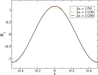
Figure 1: Magnetic field component $B_{y}$ for a large-amplitude CP Alfvén wave and for three different resolutions $\Delta x=\{1/50,1/100,1/200\}$. The conductivity is constant with a magnitude of $\sigma=10^{6}$. The agreement betweem the exact solution and that corresponding to the high resolution one is excellent.

5 Numerical tests

In this section we present several one-dimensional (1D) or two-dimensional (2D) tests which have been used to validate the implementation of the IMEX Runge-Kutta schemes in the different regimes of relativistic resistive MHD. In all these tests we employ the ideal-fluid EOS with $\Gamma=2$ for the 1D tests and $\Gamma=4/3$ in the 2D ones. The different tests span several prescriptions for the conductivity and compare the solutions obtained either with those expected in the ideal-MHD limit or with those obtained with the Strang-splitting technique.

More specifically, in 1D we consider large-amplitude circularly polarized (CP) Alfvén waves to test the ability of the code to reproduce the ideal-MHD results when adopting a very large conductivity. The intermediate conductivity regime is instead tested by simulating a self-similar current sheet. Finally, a large range of uniform and non-uniform conductivities are used for a representative shock-tube problem. In 2D, on the other hand, we first consider a commonly employed test for ideal-MHD codes corresponding to a cylindrical explosion. Subsequently, we simulate a toy model for a “magnetized neutron star” when modelled as a cylindrically symmetric density distribution obeying a Gaussian-profile. The behaviour of the magnetic field is studied again for a range of constant and non-uniform conductivities.

5.1 One-dimensional tests

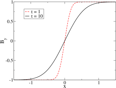
Figure 2: Magnetic field component $B_{y}$ in a self-similar current sheet. The solution is computed with $N=200$ gridpoints ($\Delta x=1/200$) and is shown at the initial time $t=1$ and at $t=10$. The conductivity is uniform with a magnitude of $\sigma=10^{2}$ (i.e., $\eta=1/\sigma=0.01$). The numerical solution is in excellent agreement with the exact one.

5.1.1 Large amplitude CP Alfvén waves

This test is discussed in detail by Del Zanna et al. (2007) and we report here only a short summary. The solution describes the propagation of a large amplitude circularly-polarized Alfvén waves along a uniform background field $B_{0}$ in a domain with periodic boundary conditions. The exact solution in the ideal-MHD limit and assuming $v_{x}=0$ for simplicity, is given by (Del Zanna et al., 2007)

$$(B_{y},B_{z}) = \eta_{A}B_{0}~{}(\cos[k(x-v_{A}~{}t)],\sin[k(x-v_{A}~{}t)])\,,$$

$$(v_{y},v_{z}) = -\frac{v_{A}}{B_{0}}~{}(B_{y},B_{z})\,,$$ (62)

where $B_{x}=B_{0}$, $k$ is the wave vector, $\eta_{A}$ is the amplitude of the wave and the special relativistic Alfvén speed $v_{A}$ is given by

$$v_{A}^{2}=\frac{2B_{0}^{2}}{h+B_{0}^{2}(1+\eta_{A}^{2})}\left(1+\sqrt{1-\left(\frac{2\eta_{A}B_{0}^{2}}{h+B_{0}^{2}(1+\eta_{A}^{2})}\right)^{2}}\right)^{-1}\,.$$ (63)

In practice, using such ideal-MHD solution it is possible to assess the accuracy of evolution of the resistive equations by requiring that for very large conductivities the numerical solution approaches the exact one as the resolution is progressively increased. It is also worth remarking that although we do not expect the solution of the resistive MHD equations to converge to that of ideal MHD for any finite value of $\sigma$, we also expect the differences between the two to be ${\cal O}(v/\sigma)$ and thus negligibly small for sufficiently large values. For this reason, we have performed the evolution with a high uniform conductivity of $\sigma=10^{6}$ for three different resolutions $N=\{50,100,200\}$ covering the computational domain $x\in[-0.5,0.5]$. In addition, the initial data parameters have been chosen so that $\rho=p=\eta_{A}=1$ and $B_{0}=1.1547$, thus yielding $v_{A}=1/2$, with a full period being achieved at $t=2$.

         

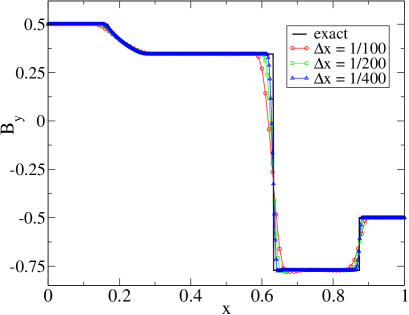
Figure 3: Left panel: Magnetic field component $B_{y}$ in the solution of the shock-tube problem. Different lines refer to three different resolutions and to the exact ideal-MHD solution at $t=0.4$. The conductivity is uniform with a magnitude of $\sigma_{0}=10^{6}$. Right panel: The same as in the left panel but for different uniform conductivities. Note that for $\sigma_{0}=0$ the solution describes a discontinutiy propagating at the speed of light and corresponding to Maxwell equations in vacuum. As the conductivity increases, the solution tends to the ideal-MHD one.

Fig. 1 confirms this expectation by reporting the component $B_{y}$ after one period and thus overlapping with the initial one (at $t=0$) for the highest resolution. This test shows clearly that in the limit of very high conductivity the resistive MHD equations tend to a solution which is very close to the same solution obtained in the ideal-MHD limit. The convergence rate measured for the different fields is consistent with the second-order spatial discretization being used as expected for smooth flows (see Appendix A).

5.1.2 Self-similar current sheet

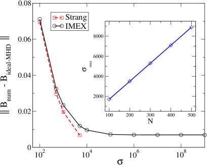
Figure 4: Differences in the magnetic field component $B_{y}$ between the numerical solution computed with either the Strang or the IMEX schemes and the exact solution of the shock-tube in the ideal-MHD limit. The differences are computed for several uniform conductivities, although the Strang-splitting technique does not yield a stable solution for values larger than $\sigma_{0}\sim 7000$ for the reference resolution of $\Delta x=1/400$ (i.e. with $400$ gridpoints). Shown in the inset is the maximum conductivity for which a solution was possible, $\sigma_{\rm max}$, as a function of the number of gridpoints, $N$.

The details of this test are described by Komissarov (2007), so again we provide here only a short description for completeness. We assume that the magnetic pressure is much smaller than the fluid pressure everywhere, with a magnetic field given by ${\boldsymbol{B}}=(0,B_{y}(x,t),0)$, where $B_{y}(x,t)$ changes sign within a thin current layer of width $\Delta l$. Provided the initial solution is in equilibrium ($p={\rm const.}$), the evolution is a slow diffusive expansion of the layer due to the resistivity and described by the diffusion equation [cf. Eq. (28) with ${\boldsymbol{v}}=0$]

$$\partial_{t}B_{y}-\frac{1}{\sigma}\partial_{x}^{2}B_{y}=0~{}~{}.$$ (64)

As the system expands, the width of the layer becomes much larger than $\Delta l$ and it evolves in a self-similar fashion. For $t>0$, the analytical exact solution is given by

$$B_{y}(x,t)=B_{0}\,{\rm erf}\,\left(\frac{1}{2}\sqrt{\frac{\sigma}{\xi}}\right)\,,$$ (65)

where $\xi=t/x^{2}$ and “${\rm erf}$” is the error function. This solution can be used for testing the moderate resistive regime. Following Komissarov (2007), and in order to avoid the singular behaviour at $t=0$, we have chosen as initial data the solution at $t=1$ with $p=50$, $\rho=1$, $E={\boldsymbol{v}}=0$ and $\sigma=100$. The domain covers the region $x\in[-1.5,1.5]$ with $N=200$ points.

         

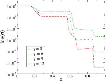
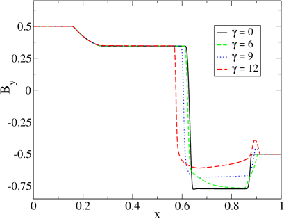
Figure 5: Left panel: Evolution of a non-uniform conductivity $\sigma$ in the shock-tube problem for different values of $\gamma$ and indicated by the different lines ($\sigma_{0}=10^{6}$ for all lines). Notice the large variability on the magnitude of the conductivity. Right panel: The same as in the left panel but for the magnetic field component $B_{y}$.

The numerical simulation is evolved up to $t=10$ and then the numerical and the exact solution are compared in Fig. 2. The two solutions match so well that they are not distinguishable on the plot, thus, showing that the intermediate-conductivity regime is also well described by our method.

5.1.3 Shock-tube problem

As prototypical shock-tube test we consider a simple MHD version of the Brio and Wu test (Brio & Wu, 1988), where the initial left and right states are separated at $x=0.5$ and are given by

$$(\rho^{L},p^{L},B_{y}^{L}) = (1.0,1.0,0.5)\,,$$

$$(\rho^{R},p^{R},B_{y}^{R}) = (0.125,0.1,-0.5)\,,$$

while all the other fields set to $0$. We consider both uniform and non-uniform conductivities. In the latter case we adopt the following prescription

$$\sigma=\sigma_{0}D^{\gamma}\,,$$ (66)

thus allowing for nonlinearities in the dependence of the conductivity on the conserved quantity $D$. This is one of the simplest cases, but in realistic situations a more general expression for the conductivity can be assumed, where $\sigma$ is a function of both the rest-mass density and of the specific internal energy, i.e., $\sigma=\sigma(\rho,\epsilon)$.

The exact solution of the ideal MHD Riemann problem was found by (Giacomazzo & Rezzolla, 2006), and in our particular case it has been computed with a publicly available code [see Giacomazzo & Rezzolla (2006)]. When $B_{x}=0$, the structure of the solution contains only two fast waves, a rarefaction moving to the left and a shock moving to the right, with a tangential discontinuity between them. More demanding Riemann problems have also been performed but the procedure to convert the conserved variables into the primitive ones has shown in these case a lack of robustness for large ratios of $|{\boldsymbol{B}}|^{2}/p$.

We have first considered the case of uniform ($\gamma=0$) and very large conductivity ($\sigma_{0}=10^{6}$) as in this case we can use the solution in the ideal-MHD limit as a useful guide. The profile of the magnetic field component $B_{y}$ for three different resolutions $\Delta x=\{1/100,1/200,1/400\}$ and the exact solution are shown in the left panel of Fig. 3 at $t=0.4$. Overall, the results indicate that even in the presence of shocks our numerical solution of the resistive MHD tends to the ideal-MHD solution as the resolution is increased. It is also interesting to study the behaviour of the solution for different values of the constant $\sigma_{0}$ while still keeping a uniform conductivity (i.e., $\gamma=0$). This is shown in the right panel of Fig.3, which displays the different solutions obtained, and where it is possible to see how they change smoothly from a wave-like solution for $\sigma_{0}=0$ to the ideal-MHD one for $\sigma_{0}=10^{6}$.

This set up is also useful to perform a comparison between the IMEX and the Strang-splitting approaches. In Fig. 4 we show the $L^{1}$-norm of the difference between the numerical solution obtained with both schemes and the ideal-MHD exact solution, for different values of the conductivity with $N=400$ points.

Several comments are in order. Firstly, the reported difference between the numerical solution for the resistive MHD equations and the ideal-MHD equations should not be interpreted as an error given that the latter is not the correct solution of the equations. Hence, the fact that the use of a Strang-splitting method yields smaller differences is simply a measure of its ability of better capture steep gradients. Secondly, while the IMEX approach does not show any sign of instability for $\sigma_{0}$ ranging between $10^{2}$ and $10^{9}$, the implementation adopting the Strang-splitting technique becomes unstable for moderately high values of the conductivity and, at least for the shock-tube problem, no numerical solution was possible for $\sigma_{0}\gtrsim 7000$ at the above resolution. Increasing the resolution can help increase the maximum value of the resistivity which can be handled, but since this gain is only linear with the number of gridpoints aiming for higher conductivities results impractical. This is shown in the inset of Fig. 4, which reports the maximum conductivity for which a solution was possible, $\sigma_{\rm max}$, as a function of the number of gridpoints, $N$. Finally, we note that the difference between the IMEX numerical solution and the exact ideal-MHD one saturates between $\sigma_{0}\sim 10^{5}-10^{6}$. This is not surprising since the differences are expected to be ${\cal O}(1/\sigma)$, and thus the saturation in the differences essentially provides a measure of our truncation error at the resolution used.

A more challenging test is offered by the solution of the shock-tube in the presence of a non-uniform conductivity. In particular, we have considered the same initial states and the same non-uniform conductivity discussed above, but used different values for the exponent $\gamma$ in (66) while keeping $\sigma_{0}$ constant. The results of this test are shown in the left panel of Fig. 5, where the conductivity is plotted at $t=0.4$ for several values of $\gamma$. Note that the conductivity traces the evolution of the rest-mass density and that the solution can be found also when $\sigma$ varies of almost $12$ orders of magnitude across the grid. Similarly, the right panel of Fig. 5 displays the component $B_{y}$ for the different values of $\gamma$. It should be stressed that because of the relation (66) between $\sigma$ and $\rho$, the region on the left has at this time a very high conductivity and the numerical solution tends to the ideal-MHD one. The opposite happens on the right region, where the conductivity is lower for higher values of $\gamma$. Clearly, the results presented in Fig. 5 show that our implementation can handle non-uniform (and quite steep) conductivity profiles even in the presence of shocks.

         

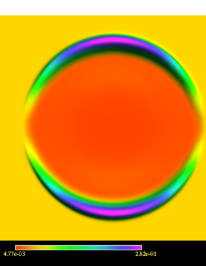
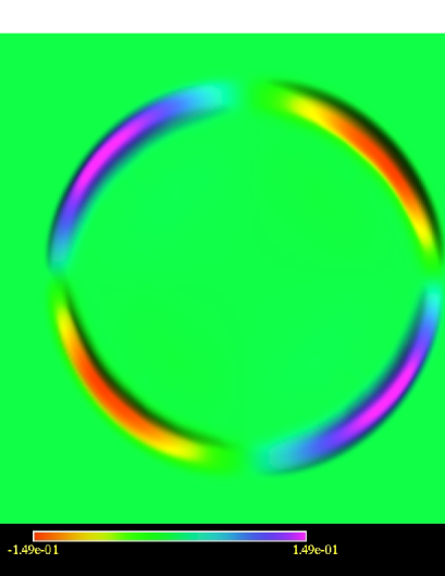
Figure 6: Magnetic field components $B_{x}$ (left panel) and $B_{y}$ (right panel) for the cylindrical explosion test at time $t=4$.

5.2 Two-dimensional tests

5.2.1 The cylindrical explosion

We now consider problems involving shocks in more than one dimension. A demanding test for the relativistic codes is the cylindrical blast wave expanding in a plasma with an initially uniform magnetic field. Although there is no exact solution for this problem, strong symmetric explosions are useful tests since shocks are present in all the possible directions and the numerical implementation is therefore tested in all of its parts. For this test we set a square domain $(x,y)\in[-6,6]$ with a resolution $\Delta x=\Delta y=1/200$. The initial data is such that inside the radius $r<0.8$ the pressure is set to $p=1$ while the density to $\rho=0.01$. In the intermediate region $0.8\leq r\leq 1.0$ the two quantities decrease exponentially up to the exterior region $r>1$, where the ambient fluid has $p=\rho=0.001$. The magnetic field is uniform with only one nontrivial component ${\boldsymbol{B}}=(0.05,0,0)$. The other fields are set to be zero (i.e., ${\boldsymbol{E}}=q=0$), which is consistent within the ideal-MHD approximation.

The evolution is performed with a high conductivity $\sigma=10^{6}$ in order to recover the solution from the ideal-MHD approximation. As shown in Fig. 6, which reports the magnetic field components $B_{x}$ (left panel) and $B_{y}$ (right panel) at time $t=4$, we obtain results that are qualitatively similar to those published in different works (Komissarov, 1999a; Neilsen et al., 2006; Del Zanna et al., 2007; Komissarov, 2007). While a strict comparison with an exact solution is not possible in this case, the solution found matches extremely well the one obtained with another 2D code solving the ideal MHD equations. Most importantly, however, the figure shows that the solution is regular everywhere and that similar results can be obtained also with smaller values of the conductivity (e.g., no significant difference was seen for $\sigma\gtrsim 10^{4}$).

5.2.2 The cylindrical star

We next consider a toy model for a star, thought as an infinite column of fluid aligned with the $z$-axis but with compact support in other directions. Because of the symmetry in the $z$-direction, $\partial_{z}\boldsymbol{U}=0$ for all the fields and the problem is therefore two-dimensional. More specifically, we consider initial data given by

$$\rho = \rho_{o}e^{-(r/r_{o})^{2}}\,,$$ (67)

$${\boldsymbol{v}} = (v^{r},v^{\phi},v^{z})=\rho~{}(0,\omega^{\phi},0)\,,$$ (68)

$${\boldsymbol{B}} = (B^{r},B^{\phi},B^{z})=\rho~{}\left(0,0,2~{}B_{o}~{}(1-\frac{r^{2}}{r_{o}^{2}})\right)\,,$$ (69)

where $r\equiv\sqrt{x^{2}+y^{2}}$ is the cylindrical radial coordinate. The other fields can be computed at the initial time by using the polytropic EOS $p=\rho^{\Gamma}$, the ideal-MHD expression (24) for the electric field, and the electric charge from the constraint equation $q=\nabla\cdot{\boldsymbol{E}}$. We have chosen $r_{o}=0.7$, $\rho=1.0$, $\omega^{\phi}=0.1$ and $B_{0}=0.05$. An atmosphere ambient fluid with $\rho=0.01$ is added outside the cylinder. Finally, the resolution is $\Delta x=1/200$ and the domain is $(x,y)\in[-3,3]$.

This simple problem exhibits some of the issues present in a magnetized rotating neutron star: a compactly supported rest-mass density distribution, an azimuthal velocity field and a poloidal magnetic field. Suitable source terms describing a gravitational potential have been added to the Euler equations in order to get, at least at the initial time, a stationary solution. In the ideal-MHD limit the magnetic lines are frozen in the fluid and thus a static profile is also expected for the magnetic field.

In the left panel of Fig. 7 we plot the slice $y=0$ of the magnetic field component $B^{z}$ at $t=14$ as obtained from the evolution of the resistive MHD system for different uniform conductivities in the range $\sigma_{0}~{}\epsilon~{}[10^{2},10^{6}]$. In the limiting case $\sigma_{0}=0$ the solution corresponds to a wave propagating at the speed of light (i.e., the solution of the Maxwell equations in vacuum), while for large values of $\sigma_{0}$ the solution is stationary (as expected in the ideal-MHD limit). The behaviour observed in the left panel Fig. 7 is also the expected one: the higher the conductivity, the closer the solution is to the stationary solution of the ideal-MHD limit. For low conductivities, on the other hand, there is a significant diffusion of the solution, which is quite rapid for $\sigma_{0}<10^{2}$ and for this reason those values are not plotted here. We note that values of the conductivity larger than $\sigma_{0}>10^{7}$ lead to numerical instabilities that we believe are coming from inaccuracies in the evolution of the charge density $q$, and which contains spatial derivatives of the current vector. In addition, the stiff quantity $E_{x}$ is seen to converge only to an order $\sim 1.5$. This can be due to the “final layer” problem of the IMEX methods, which is known to produce a degradation on the accuracy of the stiff quantities. Luckily, this does not spoil the convergence of the non-stiff fields, which are instead second-order convergent. It is possible that the use of stiffly-accurate schemes can solve this degradation of the convergence and this is an issue we are presently exploring.

         

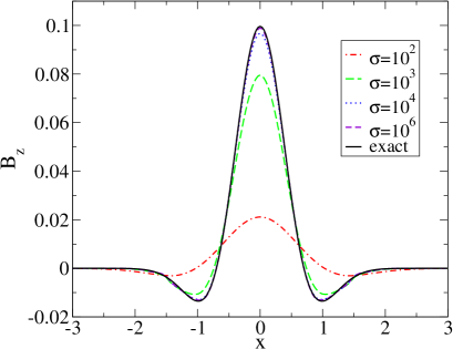
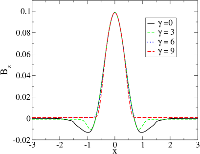
Figure 7: Left panel: Slice, at $y=0$, of the magnetic field component $B^{z}$ for different conductivities $\sigma$ and the exact solution in the ideal-MHD limit. The resolution is $\Delta x=1/200$ and the solution is plotted at $t=14$. Right panel: the same configuration as in the left panel but with a non-uniform conductivity with $\sigma_{0}=10^{6}$ and $\gamma=[0,3,6,9]$. The values inside the star are essentially the same for any $\gamma$, while there are significant differences outside.

We finally consider the same test, but now employing the non-uniform conductivity given by Eq. (66) with $\sigma_{0}=10^{6}$ and different values for $\gamma$. The results are presented in the right panel of Fig. 7, which shows that the magnetic fields inside the star are basically the same in all the cases, stressing the fact that the interior of the star will not be significantly affected by the exterior solution, which has much smaller conductivity. However, the electromagnetic fields outside the star do change significantly for different values of $\gamma$, underlining the importance of a proper treatment of the resistive effects in those regions of the plasma where the ideal-MHD approximation is not a good one.

6 Conclusions

We have introduced Implicit-Explicit Runge-Kutta schemes to solve numerically the (special) relativistic resistive MHD equations and thus deal, in an effective and robust way, with the problems inherent to the evolution of stiff hyperbolic equations with relaxation terms. Since for these methods the only limitation on the size of the timestep is set by the standard CFL condition, the approach suggested here allows to solve the full system of resistive MHD equations efficiently without resorting to the commonly adopted limit of the ideal-MHD approximation.

More specifically, we have shown that it is possible to split the system of relativistic resistive MHD equations into a set of equations that involves only non-stiff terms, which can be evolved straightforwardly, and a set involving stiff terms, which can also be solved explicitly because of the simple form of the stiff terms. Overall, the only major difficulty we have encountered in solving the resistive MHD equations with IMEX methods arises in the conversion from the conserved variables to the primitive ones. In this case, in fact, there is an extra difficulty given by the fact that there are four primitive fields which are unknown and have to be inverted simultaneously. We have solved this problem by using extra iterations in our 1D Newton-Raphson solver, but a multidimensional solver is necessary for a more robust and efficient implementation of the inversion process.

With this numerical implementation we have carried out a number of numerical tests aimed at assessing the robustness and accuracy of the approach, also when compared to other equivalents ones, such as the Strang-splitting method recently proposed by Komissarov (2007). All of the tests performed have shown the effectiveness of our approach in solving the relativistic resistive MHD equations in situations involving both small and large uniform conductivities, as well as conductivities that are allowed to vary nonlinearly across the plasma. Furthermore, when compared with the Strang-splitting technique, the IMEX approach has not shown any of the instability problems that affect the Strang-splitting approach for flows with discontinuities and large conductivities.

While the results presented here open promising perspectives for the implementation of IMEX schemes in the modelling of relativistic compact objects, at least two further improvements can be made with minor efforts. The first one consists of the generalization of the (special) relativistic resistive MHD equations with a scalar isotropic Ohm’s law to the general relativistic case, and its application to compact astrophysical bodies such a magnetized binary neutron stars (Anderson et al., 2008; Liu et al., 2008). The solution of the resistive MHD equations can yield different results not only in the dynamics of the magnetosphere produced after the merger, but also provide the possibility to predict, at least in some approximation, the electromagnetic radiation produced by the merger of these objects. The second improvement consists of considering a non-scalar and anisotropic Ohm’s law, so that the behaviour of the currents in the magnetosphere can be described by using a very high conductivity along the magnetic lines and a negligibly small one in the transverse directions (Komissarov, 2004). Such an improvement may serve as a first step towards an alternative modelling of force-free plasmas.

Appendix A TVD space discretization

We are generically interested in solving hyperbolic conservation laws of the form

$$\partial_{t}\boldsymbol{U}+\partial_{k}~{}^{k}{\boldsymbol{F}}(\boldsymbol{U})={\boldsymbol{S}}(\boldsymbol{U})\,,$$ (70)

where $\boldsymbol{U}$ is the vector of the evolved fields, ${}^{k}{\boldsymbol{F}}$ are their fluxes and ${\boldsymbol{S}}$ contains the sources terms. The semi-discrete version of this equation, in one dimension, is simply given by

$$\partial_{t}\boldsymbol{U}_{i}=-\frac{\boldsymbol{\hat{F}}_{i+1/2}-\boldsymbol{\hat{F}}_{i-1/2}}{\Delta x}+{\boldsymbol{S}}(\boldsymbol{U}_{i})\,,$$ (71)

where $\boldsymbol{\hat{F}}_{i\pm 1/2}$ are consistent numerical fluxes evaluated at the interfaces between numerical cells. These consistent fluxes are computed by using HRSC methods, which are based on the use of Riemann solvers. More specifically, we have implemented a modification of the Local Lax-Friedrichs approximate Riemann solver introduced by Alic et al. (2007), which only needs the spectral radius (i.e., the maximum eigenvalue) of the system. In highly relativistic cases, like the ones we are interested in, the spectral radius is close to the light speed $c=1$ and so the Local Lax-Friedrichs reduces to the simpler Lax-Friedrichs flux

$${\hat{F}}_{i+1/2}=\frac{1}{2}[F_{L}+F_{R}+(u_{L}-u_{R})]\,,$$ (72)

where $u_{L},u_{R}$ are the reconstructed solutions on the left and on the right of the interface and $F_{L},F_{R}$ their corresponding fluxes. The standard procedure is then to reconstruct the solution $u_{L},u_{R}$ by interpolating with a polynomial and then compute the fluxes $F_{L}=F(u_{L})$ and $F_{R}=F(u_{R})$. In our implementation we first recombine the fluxes and the solution as (Alic et al., 2007)

$${F}_{i}^{\pm}={F}_{i}\pm u_{i}\,.$$ (73)

Then, using a piecewise linear reconstruction, these combinations can be computed on the left/right of the interface as

$${F}_{L}^{+}={F}_{i}^{+}+\frac{1}{2}\Delta_{i}^{+}\,,\hskip 28.45274pt{F}_{R}^{-}={F}_{i+1}^{-}-\frac{1}{2}\Delta_{i+1}^{-}\,,$$ (74)

where $\Delta_{i}^{\pm}$ are just the slopes used to extrapolate $F_{i}^{\pm}$ to the interfaces. Finally, the consistent flux is computed by a simple average

$${\hat{F}}_{i+1/2}=\frac{1}{2}[F_{L}^{+}+F_{R}^{-}]\,.$$ (75)

For a linear reconstruction the slopes can be written as

$${\Delta}_{i}^{+} = L({F}_{i+1}^{+}-{F}_{i}^{+},{F}_{i}^{+}-{F}_{i-1}^{+})\,,$$

$${\Delta}_{i+1}^{-} = L({F}_{i+2}^{+}-{F}_{i+1}^{+},{F}_{i+1}^{+}-{F}_{i}^{+})\,,$$ (76)

so that it is trivial to check that the standard Lax-Friedrichs (72) is recovered when $\Delta_{i}^{+}=\Delta_{i}^{-}$. The choice of these slopes becomes crucial in the presence of shocks or very sharp profiles, while the use of some nonlinear operators $L(x,y)$ preserves the Total Variation Diminishing (TVD) condition on the interpolating polynomial. In this way, the TVD schemes capture accurately the dynamics of strong shocks without the oscillations which appear with standard finite-difference discretizations. Monotonicity is typically enforced by making use of slope limiters and we have in particular implemented the Monotonized Centered (MC) limiter

$$L(x,y)=\frac{1}{2}[{\rm sign}(x)+{\rm sign}(y)]~{}{\rm min}(2|x|,2|y|,\frac{1}{2}|x+y|)\,,$$ (77)

which provides a good compromise between robustness and accuracy. Note that with linear reconstruction the scheme is second-order accurate in the smooth regions, although it drops to first order near shocks and at local extrema.

References

- Alic et al. (2007) Alic D., Bona C., Bona-Casas C., Masso J., 2007, Phys. Rev. D., 76, 104007
- Anderson et al. (2008) Anderson M., Hirschmann E., Lehner L., Liebling S., Motl P., Neilsen D., Palenzuela C., Tohline J., 2008, Phys. Rev. Lett., 100, 191101
- Anile (1989) Anile A., 1989, Relativistic fluids and magneto-fluids: With applications in astrophysics and plasma physics, Cambridge Monographs on Mathematical Physics. Cambridge University Press, Cambridge, U.K.; New York, U.S.A.
- Anninos et al. (2005) Anninos P., Fragile P., Salmonson J., 2005, Astrophys. J., 635, 723
- Anton et al. (2006) Anton L., Zanotti O., Miralles J., Marti J., Ibanez J., Font J., Pons J., 2006, Astrophys. J., 637, 296
- Asher et al. (1997) Asher U., Ruuth S., Spiteri R., 1997, Appl. Numer. Math., 25, 151
- Asher et al. (1995) Asher U., Ruuth S., Wetton B., 1995, SIAM J. Numer. Anal., 32, 797
- Brio & Wu (1988) Brio M., Wu C., 1988, J. Computat. Phys., 75, 400
- Butcher (1987) Butcher J., 1987, The Numerical Analysis of Ordinary Differential Equations: Runge-Kutta and General Linear Methods. John Wiley and Sons
- Butcher (2003) —, 2003, Numerical methods for ordinary differential equations. John Wiley and Sons
- Carter (1991) Carter B., 1991, Proc. R. Soc. London, Ser. A, 433, 45
- Chen et al. (1994) Chen G., Levermore D., Liu T., 1994, Comm. Pure Appl. Math., 47, 787
- Dedner et al. (2002) Dedner A., Kemm F., Kroner D., Munz C., Schnitzer T., Wesenberg M., 2002, J. Computat. Phys., 175, 645
- Del Zanna et al. (2003) Del Zanna L., Bucciantini N., Londrillo P., 2003, Astron. and Astrophys., 400, 397
- Del Zanna et al. (2007) Del Zanna L., Zanotti O., Bucciantini N., Londrillo P., 2007, Astron. and Astrophys., 473, 11
- Duez et al. (2005) Duez M., Tung Liu Y., Shapiro S., Stephens B., 2005, Phys. Rev. D., 72, 024028
- Farris et al. (2008) Farris B., Ka Li T., Tung Liu Y., Shapiro S., 2008, Phys. Rev. D., 78, 024023
- Gammie et al. (2003) Gammie C., McKinney J., Toth G., 2003, Astrophys. J., 589, 444
- Giacomazzo & Rezzolla (2006) Giacomazzo B., Rezzolla L., 2006, J. Fluid Mech., 562, 223
- Giacomazzo & Rezzolla (2007) —, 2007, Classical and Quantum Gravity, 24, S235
- Gottlieb et al. (2001) Gottlieb S., Shu C., Tadmor E., 2001, SIAM Review, 43, 89
- Graves et al. (2008) Graves D. T., Trebotich D., Miller G., Colella P., 2008, Journal of Computational Physics, 227, 4797
- Israel (1976) Israel W., 1976, Ann. Phys., 100, 310
- Jahnke & Lubich (2000) Jahnke J., Lubich C., 2000, BIT, 735
- Koide et al. (1999) Koide S., Shibata K., Kudoh T., 1999, Astrophys. J., 522, 727
- Koldoba et al. (2002) Koldoba A., Romanova M., Ustyugova G., Lovelace R., 2002, Astrophys. J., 576, 445
- Komissarov (1999a) Komissarov S. S., 1999a, Mon. Not. R. Astron. Soc., 303, 343
- Komissarov (1999b) —, 1999b, Mon. Not. R. Astron. Soc., 308, 1069
- Komissarov (2001) —, 2001, Mon. Not. R. Astron. Soc., 326, L41
- Komissarov (2002) —, 2002, Mon. Not. R. Astron. Soc., 336, 759
- Komissarov (2004) —, 2004, Mon. Not. R. Astron. Soc., 350, 427
- Komissarov (2007) —, 2007, Mon. Not. R. Astron. Soc., 382, 995
- Komissarov et al. (2007) Komissarov S. S., Barkov M., Lyutikov M., 2007, Mon. Not. R. Astron. Soc., 374, 415
- Lamb (1991) Lamb F. K., 1991, in Frontiers of Stellar Evolution, Lambert D. L., ed., Astronomical Society of the Pacific, San Francisco, p. 299
- Landau & Lifshitz (1980) Landau L., Lifshitz E., 1980, The Classical Theory of Fields. Butterworth-Heinemann
- Lichnerowicz (1967) Lichnerowicz A., 1967, Relativistic hydrodynamics and magnetohydrodynamics. Benjamin, New York
- Liu et al. (2008) Liu Y., Shapiro S., Zachariah B., Taniguchi K., 2008, Phys. Rev. D., 78, 024012
- McKinney (2006a) McKinney J. C., 2006a, MNRS, 367, 1797
- McKinney (2006b) —, 2006b, Mon. Not. Roy. Astron. Soc., 368, 1561
- Mignone & Bodo (2006) Mignone A., Bodo G., 2006, Mon. Not. R. Astron. Soc., 368, 1040
- Neilsen et al. (2006) Neilsen D., Hirschmann E., Millward R., 2006, Class. Quant. Grav., 23, S505
- Noble et al. (2007) Noble S. C., Leung P. K., Gammie C. F., Book L. G., 2007, Class. Quant. Grav., 24, S259
- Pareschi (2001) Pareschi L., 2001, SIAM J. Num. Anal, 39, 1395
- Pareschi & Russo (2005) Pareschi L., Russo G., 2005, J. Sci. Comput., 25, 112
- Potekhin et al. (1999) Potekhin A. Y., Baiko D. A., Haensel P., Yakovlev D. G., 1999, Astron. and Astrophys., 346, 345
- Reynolds et al. (2006) Reynolds D., Samtaney R., Woodward C., 2006, Journal of Computational Physics, 219, 144
- Shibata & Sekiguchi (2005) Shibata M., Sekiguchi Y., 2005, Phys. Rev. D., 72, 044014
- Spiteri & Ruuth (2002) Spiteri R., Ruuth S., 2002, SIAM J. Numer. Anal., 40(2), 469
- Stewart (1977) Stewart J., 1977, Proc. Roy. Soc. (London) A., 365, 43
- Strang (1968) Strang G., 1968, SIAM J. Numer. Anal., 5, 505