Relativistic MHD in dynamical spacetimes:
Improved EM gauge condition for AMR grids

Abstract

We recently developed a new general relativistic magnetohydrodynamic code with adaptive mesh refinement that evolves the electromagnetic (EM) vector potential $A_{i}$ instead of the magnetic fields directly. Evolving $A_{i}$ enables one to use any interpolation scheme on refinement level boundaries and still guarantee that the magnetic field remains divergenceless. As in classical EM, a gauge choice must be made when evolving $A_{i}$, and we chose a straightforward “algebraic” gauge condition to simplify the $A_{i}$ evolution equation. However, magnetized black hole-neutron star (BHNS) simulations in this gauge exhibit unphysical behavior, including the spurious appearance of strong magnetic fields on refinement level boundaries. This spurious behavior is exacerbated when matter crosses refinement boundaries during tidal disruption of the NS. Applying Kreiss-Oliger dissipation to the evolution of the magnetic vector potential $A_{i}$ slightly weakens this spurious magnetic effect, but with undesired consequences. We demonstrate via an eigenvalue analysis and a numerical study that zero-speed modes in the algebraic gauge, coupled with the frequency filtering that occurs on refinement level boundaries, are responsible for the creation of spurious magnetic fields. We show that the EM Lorenz gauge exhibits no zero-speed modes, and as a consequence, spurious magnetic effects are quickly propagated away, allowing for long-term, stable magnetized BHNS evolutions. Our study demonstrates how the EM gauge degree of freedom can be chosen to one’s advantage, and that for magnetized BHNS simulations the Lorenz gauge constitutes a major improvement over the algebraic gauge.

I Introduction

Magnetized fluids in dynamical, strongly curved spacetimes play a central role in many systems of current interest in relativistic astrophysics. The presence of magnetic fields may destroy differential rotation in nascent neutron stars, form jets and influence disk dynamics around black holes, affect collapse of massive rotating stars, etc. Many of these systems are promising sources of gravitational radiation for detection by laser interferometers such as LIGO, VIRGO, TAMA, GEO, LCGT, ET, LISA and DECIGO. Some may also emit electromagnetic radiation as gamma-ray bursts, or emission from magnetized disks around black holes in active galactic nuclei and quasars. Accurate, self-consistent modeling of these systems requires computational schemes capable of simultaneously accounting for magnetic fields, relativistic magnetohydrodynamics (MHD), radiation transport and relativistic gravitation.

Over the past several years, we have developed a numerical scheme in 3+1 dimensions capable of solving the coupled system of Einstein’s field equations, relativistic MHD and Maxwell’s equations DSY04 ; ELS2010 . Our approach is based on the BSSN (Baumgarte-Shapiro-Shibata-Nakamura) formalism to evolve the metric SN ; BS , a high-resolution, shock-capturing (HRSC) scheme to handle the fluids, and a constrained-transport (CT) scheme to treat the magnetic induction equation toth . This GRMHD code has been subjected to a rigorous suite of numerical tests to check and calibrate its accuracy DSY04 ; ELS2010 . The code has been applied to explore a number of important dynamical scenarios in relativistic astrophysics, including the collapse of magnetized, differentially rotating hypermassive neutron stars to black holes dlsss06a ; dlsss06b ; SSL08 , the collapse of rotating stellar cores to neutron stars ShiUIUC , the collapse of rotating, supermassive stars and massive Population III stars to black holes lss07 , magnetized binary neutron star merger lset08 , binary black hole-neutron stars (BHNSs) eflstb08 ; elsb09 , binary white dwarf-neutron stars PELS11 ; PLES11 , and the merger of binary black holes in gaseous clouds FLS10 and disks FLS11 .

Many problems in relativistic astrophysics require numerical simulations covering a large range of length scales. For example, to follow the final merger of a compact binary system with a total mass $M$, length scales of $M/30$ or less must be resolved to treat the strong-field, near-zone regions reliably. On the other hand, accurate gravitational wave calculations at length scales $\sim M$ must be performed far in the weak-field wave-zone at radius $r\gtrsim 100M$. Adaptive mesh refinement (AMR) allows for sufficient resolution to be supplied to areas of the computational domain as needed, enabling us to resolve both strong- and weak-field domains efficiently.

One of the most subtle issues in evolving the MHD equations is the preservation of the divergenceless constraint ($\mathbf{\nabla\cdot B}=0$). When evolving the induction equation, numerical truncation error leads to violations of this constraint, resulting in unphysical plasma transport orthogonal to the magnetic field, as well as violations of energy and momentum conservation (see e.g., toth ; BB80 ; BS99 ). In simulations using a uniformly-spaced grid, constrained-transport schemes (see e.g., eh88 ; toth ) are commonly used to maintain the divergenceless constraint. In simulations using AMR grids, both CT schemes and the hyperbolic divergence-cleaning (HDC) method DKKMSW02 ; AHLS06 have been used. However, we find that in the presence of black holes, otherwise stable GRMHD evolution schemes often become unstable.

One of the most commonly adopted methods for evolving black holes is the moving puncture technique RIT1 ; God1 , in which the puncture gauge conditions ensure that the spacetime singularity in the black hole interior never appears. However, a coordinate singularity is present in the computational domain near which accurate numerical evolution is difficult to achieve. It has been demonstrated that when using the moving puncture gauge, while gauge modes can leak out of the BH horizon Brown09 , any physical or constraint violating data in the black hole interior will not propagate out of the horizon EFLSB ; Turducken ; Turducken2 . We find that this property is preserved in the presence of hydrodynamic matter, but can be challenging to maintain when the matter is magnetized. Though we have found that the HDC scheme works well with the moving puncture technique in the absence of black holes, when BHs are present and excision is not applied, we find that, even in the Cowling approximation, in which the metric is fixed, inaccurate data in the black hole interior can propagate out of the horizon and contaminate the solutions.

For this reason, in developing a moving puncture-compatible algorithm for maintaining $\mathbf{\nabla\cdot B}=0$, we focused on CT schemes. This was the approach adopted in our earlier, unigrid GRMHD code DSY04 . In AMR simulations, the conventional CT scheme may be used where individual refinement levels do not overlap. However, maintaining the divergenceless constraint at refinement level boundaries requires that special interpolations be performed during prolongation and restriction. Such prolongation/restriction operators have been devised Balsara01 ; Balsara09 ; McNally11 , but these operators must be fine-tuned to the particular AMR implementation, and some have only been tested for Newtonian MHD.

In ELS2010 we developed an alternative, AMR-compatible CT scheme. The scheme is based on the CT method described in zbl03 , which recasts the magnetic induction equation as an evolution equation for the magnetic vector potential. Divergence-free magnetic fields are guaranteed as they are computed from the curl of the vector potential. The evolution of the vector potential is carried out in the same HRSC framework as other hydrodynamic variables. This scheme is numerically equivalent to the commonly-used, staggered-$B$ CT scheme of BS99 for uniform resolution simulations, but is readily generalized to an AMR grid. Unlike the magnetic field, the vector potential is not constrained, so any interpolation scheme may be used during prolongation and restriction, thus enabling its use with any AMR algorithm. In addition, since the vector potential does not uniquely determine the magnetic field, there exists an extra gauge degree of freedom that can be used to one’s advantage. A straightforward “algebraic” gauge condition was adopted in our original formulation, to simplify evolution equation for the vector potential (see also zbl03 ; grb11 ).

In ELS2010 we performed several tests on our new AMR-compatible CT scheme. We found that our scheme works well even in black-hole spacetimes. Inaccurate data generated in the black hole interior stayed inside the horizon. Hence our scheme is compatible with the moving puncture technique. However, when this algebraic gauge condition is used for magnetized binary black hole–neutron star (BHNS) simulations, stable, long-term evolutions are not possible.

In this paper, we exploit another EM gauge condition, the Lorenz gauge , which allows for stable, long-term GRMHD evolutions of binary BHNSs. Performing eigenvalue analyses, we find that static EM modes are present when adopting the algebraic gauge, whereas all EM modes are propagating when the Lorenz gauge is adopted. As a result, when the algebraic gauge is used, its zero-speed modes are inevitably excited and remain on the grid. Further, when these modes are interpolated at refinement boundaries, inaccuracies in interpolation may lead to the appearance of spurious magnetic fields that contaminate the solution and lead to a build-up of numerical error. Given that the Lorenz gauge possesses no static modes, any such spurious modes should be propagated away to the boundary and leave the grid. Thus, we expect that the solutions will be improved when using the Lorenz gauge.

Using magnetized BHNS simulations we perform a comparison between the Lorenz gauge and the algebraic gauge with and without Kreiss-Oliger dissipation (KOD) applied on the vector potential evolution. We confirm the expected behavior. The BHNS system that forms the basis of our comparison is an irrotational binary in an initially circular orbit, with a BH:NS mass ratio of 3:1 and the NS initially seeded with a small poloidal magnetic field. Using these simulations we demonstrate the superiority of the Lorenz gauge, and confirm that in the algebraic gauge static modes are present and lead to spurious B-fields which remain on the grid. This spurious effect contaminates the solution and is amplified in time, leading the simulations to break down shortly after NS tidal disruption. In contrast to the algebraic gauge, static EM modes are not present in the Lorenz gauge, and any spurious fields generated at refinement level boundaries are quickly propagated away. Overall we find that the Lorenz gauge provides a major improvement for magnetized BHNS simulations. In elpb11 , we employ the Lorenz gauge to perform a detailed study of the effects of magnetic fields in the evolution of binary BHNSs.

The remaining sections are organized as follows. In Sec. II we outline the basic GRMHD equations and provide an overview of EM gauge conditions and evolution equations. In Sec. III we perform an eigenvalue analysis of the EM evolution equations. In Sec. IV, we briefly describe the specific implementation of our GRMHD scheme. In Sec. V, we review the differences between our magnetized BHNS simulations in the algebraic and Lorenz gauges. We summarize our findings in Sec. VI.

II Basic Equations

The formulation and numerical scheme for our simulations is basically the same as in our previous work eflstb08 ; elsb09 ; ELS2010 , to which the reader may refer for details. Here we introduce our notation, summarize our method, and point out the latest changes to our numerical technique. Geometrized units ($G=c=1$) are adopted, except where stated explicitly. Greek indices denote all four spacetime dimensions (0, 1, 2, and 3), and Latin indices imply spatial parts only (1, 2, and 3).

We use the 3+1 spacetime decomposition, in which the metric has the following form:

$$ds^{2}=-\alpha^{2}dt^{2}+\gamma_{ij}(dx^{i}+\beta^{i}dt)(dx^{j}+\beta^{j}dt)\ ,$$ (1)

where $\alpha$ is the lapse function, $\beta^{i}$ the shift vector, and $\gamma_{ij}$ the three-metric on spacelike hypersurfaces of constant time $t$. We then decompose all evolution equations in 3+1 form (see e.g. BSBook for a detailed discussion and references).

II.1 Gravitational fields

We adopt the Baumgarte-Shapiro-Shibata-Nakamura (BSSN) formalism SN ; BS in which the metric evolution variables are the conformal exponent $\phi\equiv\ln(\gamma)/12$, the conformal 3-metric $\tilde{\gamma}_{ij}=e^{-4\phi}\gamma_{ij}$, three auxiliary functions $\tilde{\Gamma}^{i}\equiv-\tilde{\gamma}^{ij}{}_{,j}$, the trace $K$ of the extrinsic curvature $K_{ij}$, and the trace-free part of the conformal extrinsic curvature $\tilde{A}_{ij}\equiv e^{-4\phi}(K_{ij}-\gamma_{ij}K/3)$. Here, $\gamma={\rm det}(\gamma_{ij})$. The full spacetime metric $g_{\mu\nu}$ is related to the three-metric $\gamma_{\mu\nu}$ by $\gamma_{\mu\nu}=g_{\mu\nu}+n_{\mu}n_{\nu}$, where the future-directed, timelike unit vector $n^{\mu}$ normal to the time slice can be written in terms of the lapse $\alpha$ and shift $\beta^{i}$ as $n^{\mu}=\alpha^{-1}(1,-\beta^{i})$. The evolution equations of these BSSN variables are given by Eqs. (9)–(13) of eflstb08 . We adopt the standard puncture gauge conditions: an advective “1+log” slicing condition for the lapse and a “Gamma-freezing” condition for the shift GodGauge . The evolution equations for $\alpha$ and $\beta^{i}$ are given by Eqs. (2)–(4) of elsb09 , with the $\eta$ parameter set to $\approx 2.2/M$ in all BHNS simulations presented here, where $M$ is the ADM mass of the binary. We add a sixth-order KOD term of the form $\epsilon/64(\Delta x^{5}\partial_{x}^{(6)}+\Delta y^{5}\partial_{y}^{(6)}+\Delta z^{5}\partial_{z}^{(6)})f$ to reduce high-frequency numerical noise associated with AMR refinement interfaces. Here $f$ stands for all evolved BSSN, lapse and shift variables. We choose the strength parameter as $\epsilon=0.2$. Note that this KOD term converges to zero at fifth-order in the grid spacing so that it does not alter the convergence properties of our BSSN scheme.

II.2 Magnetohydrodynamic fields

The fundamental MHD variables include the rest-mass density $\rho_{0}$, specific internal energy $\epsilon$, pressure $P$, four-velocity $u^{\mu}$, and magnetic field $B^{\mu}=n_{\nu}F^{*\nu\mu}$. Here $F^{*\mu\nu}$ is the dual of the Faraday tensor $F^{\mu\nu}$. Note that $B^{\mu}$ is purely spatial ($B^{0}=-n_{\mu}B^{\mu}/\alpha=0$). We adopt a $\Gamma$-law equation of state (EOS) $P=(\Gamma-1)\rho_{0}\epsilon$ with $\Gamma=2$, which reduces to an $n=1$ polytropic law for the initial (cold) neutron star matter. The stress-energy tensor is given by

$$T_{\mu\nu}=(\rho_{0}h+b^{2})u_{\mu}u_{\mu}+\left(P+\frac{b^{2}}{2}\right)g_{\mu\nu}-b_{\mu}b_{\nu}\ ,$$ (2)

where $h=1+\epsilon+P/\rho_{0}$ is the specific enthalpy and

$$b_{\mu}=-\frac{P_{\mu\nu}B^{\nu}}{\sqrt{4\pi}\,n_{\nu}u^{\nu}}$$ (3)

is the magnetic field measured in fluid’s comoving frame, modulo a factor of $1/\sqrt{4\pi}$. Here $P_{\mu\nu}=g_{\mu\nu}+u_{\mu}u_{\nu}$ and $b^{2}=b^{\mu}b_{\mu}$. In the ideal MHD limit, in which the plasma is assumed to have perfect conductivity, the Faraday tensor can be written as $F^{\mu\nu}=\sqrt{4\pi}\,u_{\gamma}\epsilon^{\gamma\mu\nu\delta}b_{\delta}$.

In the standard numerical implementation of the MHD equations using a conservative scheme, it is useful to introduce the “conservative” variables $\rho_{*}$, $\tilde{S}_{i}$, $\tilde{\tau}$ and $\tilde{B}^{i}$. They are defined as

$$\rho_{*}\equiv-\sqrt{\gamma}\,\rho_{0}n_{\mu}u^{\mu}\ ,$$ (4)

$$\tilde{S}_{i}\equiv-\sqrt{\gamma}\,T_{\mu\nu}n^{\mu}\gamma^{\nu}_{~{}i}\ ,$$ (5)

$$\tilde{\tau}\equiv\sqrt{\gamma}\,T_{\mu\nu}n^{\mu}n^{\nu}-\rho_{*}\ ,$$ (6)

$$\tilde{B}^{i}\equiv\sqrt{\gamma}\,B^{i}.$$ (7)

The evolution equations for $\rho_{*}$, $\tilde{S}_{i}$ and $\tilde{\tau}$ can be derived from the conservation of baryon number $\nabla_{\mu}(\rho_{*}u^{\mu})=0$ and conservation of energy-momentum $\nabla_{\mu}T^{\mu\nu}=0$, giving rise to Eqs. (27)–(30) in ELS2010 .

II.3 Electromagnetic fields

In the ideal MHD limit, the Maxwell equation $\nabla_{\nu}F^{*\mu\nu}=0$ yields the magnetic constraint $\partial_{j}\tilde{B}^{j}=0$ and the induction equation $\partial_{t}\tilde{B}^{i}+\partial_{j}(v^{j}\tilde{B}^{i}-v^{i}\tilde{B}^{j})=0$. As shown in ELS2010 and bs03 , these equations can be rewritten by introducing the electromagnetic 4-vector potential ${\cal A}_{\mu}=\Phi n_{\mu}+A_{\mu}$, with $n^{\mu}A_{\mu}=0$. The magnetic constraint and induction equations become

$$B^{i} = \epsilon^{ijk}\partial_{j}A_{k}\ ,$$ (8)

$$\partial_{t}A_{i} = \epsilon_{ijk}v^{j}B^{k}-\partial_{i}(\alpha\Phi-\beta^{j}A_{j})\$$ (9)

where $\epsilon^{ijk}=n_{\mu}\epsilon^{\mu ijk}$ is the 3-dimensional Levi-Civita tensor. The dynamical variable in this scheme is the vector potential. The B-field in Eq. (9) and in the MHD equations is essentially replaced according to Eq. (8).

The EM evolution via the vector potential introduces an additional gauge degree of freedom. Therefore, an EM gauge choice must be made to close the system of equations.

II.3.1 Algebraic gauge

In zbl03 ; ELS2010 , the algebraic EM gauge condition

$${\Phi=\frac{1}{\alpha}\beta^{j}A_{j}=-n^{j}A_{j}}$$ (10)

is adopted because it simplifies the evolution of $A_{i}$ to

$${\partial_{t}A_{i}=\epsilon_{ijk}v^{j}B^{k}.}$$ (11)

II.3.2 Lorenz gauge

In this paper, we find that simulations of magnetized BHNSs using AMR and the algebraic gauge suffer from severe numerical errors and eventually break down due to a build-up of errors.

Improved, stable, long-term BHNS evolutions may be achieved by imposing the Lorenz gauge condition

$${\nabla_{\mu}{\cal A}^{\mu}=0,}$$ (12)

which yields the evolution equation

$$\partial_{t}(\sqrt{\gamma}\,\Phi)+\partial_{j}(\alpha\sqrt{\gamma}\,A^{j}-\sqrt{\gamma}\,\beta^{j}\Phi)=0$$ (13)

for $\Phi$.

Our numerical implementation of Eqs. (8) and (9) guarantees numerically identical $B^{i}$ regardless of EM gauge in simulations with a uniform-resolution grid. However, interpolations performed on $A_{i}$ at refinement boundaries on AMR grids will modify $A_{i}$, resulting in different $B^{i}$ on and near these boundaries, ultimately leading to different stability properties.

III Electromagnetic gauge analysis

The differences in the stability properties of the gauges considered here can be explained by the fact that the algebraic gauge possesses a static mode, whereas all modes in the Lorenz gauge are propagating. Here we perform an eigenvalue analysis of the EM field evolution equations with the algebraic and Lorenz gauges and demonstrate explicitly the existence of static modes in the former gauge.

III.1 Evolution Equations

Substituting Eq. (8) into Eq. (9) we find that the evolution of the vector potential is given by

$${\begin{split}\partial_{t}A_{i}=&\ -v^{m}\partial_{m}A_{i}+(v^{m}+\beta^{m})\partial_{i}A_{m}-\alpha\partial_{i}\Phi\\ &\ -\Phi\partial_{i}\alpha+A_{m}\partial_{i}\beta^{m}.\end{split}}$$ (14)

Writing Eq. (13) as an evolution equation for $\Phi$ we find

$$\partial_{t}\Phi = \beta^{m}\partial_{m}\Phi-\alpha\partial_{m}A^{m}+\gamma^{-1/2}\Phi\partial_{m}(\sqrt{\gamma}\beta^{m})$$

$$-\gamma^{-1/2}A^{m}\partial_{m}(\alpha\sqrt{\gamma})-\Phi\partial_{t}\ln(\sqrt{\gamma}).$$

In the limit of short-wavelength, small-amplitude perturbations about a background solution, the EM evolution equations decouple from the MHD and BSSN equations and can be analyzed separately. While the entire coupled system of the BSSN, MHD and Maxwell’s equations is quasi-linear, the $A_{i},\Phi$ partial differential equations alone are linear, as the coefficients that multiply the spatial derivatives of $A_{i}$ and $\Phi$ are not functions of $A_{i}$ and $\Phi$. For our purpose we can apply the hyperbolicity theorems for linear systems of equations GKOpdeBook ; KLpdeBook , thus we need only consider the principal parts of the evolution equations and the localization principle.

III.2 Algebraic gauge

In this gauge only the vector potential evolves dynamically and $\Phi$ is entirely determined by $A_{i}$ and the BSSN gauge variables. The principal part of the $A_{i}$ evolution equation is given by

$${\partial_{t}A_{i}\simeq-v^{m}\partial_{m}A_{i}+v^{m}\partial_{i}A_{m}.}$$ (16)

Here $\simeq$ denotes “the principal part equals”. Replacing $\partial_{i}$ by $k_{i}$, where $k_{i}$ is the spatial component of the wave vector, normalized according to $\gamma^{ij}k_{i}k_{j}=1$, we obtain

$${\partial_{t}A_{i}\simeq-v^{m}k_{m}A_{i}+v^{m}k_{i}A_{m}\equiv F_{i}}$$ (17)

We can now construct the characteristic matrix of the system: $M_{ij}=\partial F_{i}/\partial A_{j}$. For the system to be strongly hyperbolic the eigenvalues of this matrix must be real and the matrix must possess a complete set of eigenvectors . A straightforward calculation shows that the set of eigenvectors of this system is complete and the eigenvalues (or characteristic speeds) are

$${\lambda_{1}=0,\ \lambda_{2,3}=v^{m}k_{m}.}$$ (18)

Hence the system is strongly hyperbolic. However, the system possesses a static gauge mode, i.e., a mode that does not propagate. In unigrid simulations, this is not an issue since our numerical implementation of the $A_{i}$ evolution guarantees $B^{i}$ (obtained via Eq. (8)) to be equivalent to the standard staggered-$B$ CT scheme zbl03 , which evolves $B^{i}$ directly and thus does not suffer from potential EM gauge mode problems. In AMR simulations however, $A_{i}$ is interpolated between refinement levels. The static modes will remain in the computational domain where they were generated, allowing interpolation errors between refinement levels to give rise to spurious $B^{i}$ at refinement level boundaries, which subsequently propagate to the interior of the refinement boxes and affect the dynamics of system. In this way, numerical errors can build up and lead to unstable behavior. On a related note, we point out that the existence of zero modes has also been considered as an explanation for the different stability properties of different 3+1 formulations of GR AABSS2000 ; SY2002 ; PV2008 ; PHK2008 . However, the existence of zero speed modes is not always associated with unstable behavior. For example the BSSN formulation gives rise to stable numerical integrations even though it possesses a zero-speed mode.

III.3 Lorenz gauge

In this gauge both the vector and scalar potentials evolve. The principal part of the EM evolution equations in the Lorenz gauge is

$${\begin{split}\partial_{t}A_{i}\simeq&\-v^{m}\partial_{m}A_{i}+(v^{m}+\beta^{m})\partial_{i}A_{m}-\alpha\partial_{i}\Phi,\\ \partial_{t}\Phi\simeq&\ \beta^{m}\partial_{m}\Phi-\alpha\gamma^{mn}\partial_{m}A_{n}.\end{split}}$$ (19)

Using the $\partial_{i}\rightarrow k_{i}$ rule and calculating the eigensystem of the characteristic matrix we find that the matrix has a complete set of eigenvectors and its eigenvalues are

$${\lambda_{1,2}=\beta^{m}k_{m}\pm\alpha,\ \lambda_{3,4}=v^{m}k_{m}.}$$ (20)

As in the algebraic gauge, all eigenvalues are purely real. The system is strongly hyperbolic, only this time all modes are non-zero. Thus numerical errors arising from refinement boundary interpolations will propagate away.

This is precisely what we observe in our BHNS simulations and in the following sections we show explicit numerical results that demonstrate this.

Table 1: Summary of comparison runs. The third column specifies whether KOD is applied, and the fourth column indicates whether build-up of spurious $B$-field is observed. A $\checkmark$ means “Yes” and a ✗ means “No”.

Case Name	Gauge	KOD	Spurious $B^{i}$
Algebraic	Algebraic	✗	$\checkmark$
Algebraic-KO	Algebraic	$\checkmark$	$\checkmark$
Lorenz	Lorenz	✗	✗

IV Numerical Methods

IV.1 Initial data

BHNS quasiequilibrium initial data are constructed as described in TBFS07b . The particular BHNS binary chosen in our comparison of different EM gauges corresponds to Case A of elsb09 . The system consists of an initially nonspinning BH orbiting about an irrotational NS, with a 3:1 BH:NS mass ratio. The NS has a compaction of ${\cal C}=0.145$, and is constructed using an $n=1$ ($\Gamma=2$) polytropic EOS.

Given that interior NS magnetic field strengths and configurations are unknown, we choose an initial seed poloidal magnetic field via a vector potential of the form

$$A_{i} = \left(-\frac{y-y_{c}}{\varpi_{c}^{2}}\delta^{x}{}_{i}+\frac{x-x_{c}}{\varpi^{2}_{c}}\delta^{y}{}_{i}\right)A_{\varphi}$$ (21)

$$A_{\varphi} = A_{b}\varpi^{2}_{c}\max(P-P_{\rm cut},0)^{n_{b}}$$ (22)

where $(x_{c},y_{c},0)$ is coordinate location of the center of mass of the NS, $\varpi^{2}_{c}=(x-x_{c})^{2}+(y-y_{c})^{2}$, and $A_{b}$, $n_{p}$ and $P_{\rm cut}$ are free parameters. The cutoff pressure parameter $P_{\rm cut}$ confines the B-field within the neutron star to $P>P_{\rm cut}$. The parameter $n_{b}$ determines the degree of central condensation of the magnetic field. Similar profiles of initial magnetic fields have been used in numerical simulations of magnetized accretion disks (see, e.g. dhk03 ; mg04 ) and magnetized compact binaries (see, e.g. ahllmnpt08 ; grb11 ; cabllmn10 ). We set $P_{\rm cut}$ to be 4% of the maximum pressure and $n_{b}$=2. The parameter $A_{b}$ controls the strength of the initial magnetic field and can be characterized by the maximum magnetic field inside the NS, which we set here to $B=1.3\times 10^{16}G$ (assuming the NS mass is $1.4M_{\odot}$). Such seed magnetic fields are too weak to significantly perturb the initial quasiequilibrium NS, and thereby do not contribute to any significant initial gravitational field constraint violations.

IV.2 Evolution algorithms

Our methods for evolving the metric and the MHD equations are described in elsb09 and for this reason are not presented here. This section focuses solely on our treatment of the evolution of the vector potential.

Table 2: Grid configuration used in our simulations. $N_{\rm AH}$ denotes the number of grid points covering the diameter of the apparent horizon initially, and $N_{\rm NS}$ denotes the number of grid points covering the smallest diameter of the NS initially.

Grid Hierarchy (in units of $M$)(a)	Max. resolution	$N_{\rm AH}$	$N_{\rm NS}$
(203.7, 101.8, 25.46, 12.73, 6.365, 3.183, 1.591)	$M/31.4$	40	82

^(a) There are two sets of nested refinement boxes: one centered on the NS and one on the BH. This column specifies the half side length of the refinement boxes centered either on the BH or the NS.

The magnetic induction equation is evolved via the 4-vector potential using Eqs. (9) and (13). $A_{i}$ and $B^{i}$ are staggered as in ELS2010 , and $\Phi$ exists on the $(i^{+},j^{+},k^{+})$ staggered grid [all other hydrodynamic, BSSN, lapse and shift variables are stored at $(i,j,k)$], where $(i^{+},j^{+},k^{+})=(i+1/2,j+1/2,k+1/2)$. The term $-\partial_{j}(\beta^{j}\sqrt{\gamma}\,\Phi)$ in Eq. (13) is treated using a second-order upwind scheme, and Eq. (9) is handled using the finite-volume equations similar to Eqs. (63)–(65) in ELS2010 . For example, we evolve $\hat{A}_{x}$, which is staggered at $(i,j^{+},k^{+})$, by

$$\partial_{t}(\hat{A}_{x})_{i,j^{+},k^{+}} = -\hat{\cal{E}}^{x}_{i,j^{+},k^{+}}-\frac{1}{\Delta x}[(\alpha\Phi-\beta^{j}A_{j})_{i^{+},j^{+},k^{+}}$$ (24)

$$-(\alpha\Phi-\beta^{j}A_{j})_{i^{-},j^{+},k^{+}}],$$

where $i^{-}=i-1/2$, $\hat{A}_{x}$ is the line-averaged $A_{x}$ defined in Eq. (57) of ELS2010 , ${\cal E}^{i}=\epsilon^{i}{}_{jk}B^{j}v^{k}$ and $\hat{\cal{E}}^{x}$ is the line-averaged ${\cal E}^{x}$ defined in Eq. (49) of ELS2010 . In ELS2010 and zbl03 , only the first term on the right-hand side of Eq. (24) is present because the algebraic gauge Eq. (10) is imposed. The term ${\cal E}^{x}_{i,j^{+},k^{+}}$ is computed using the HRSC scheme described in ELS2010 and zbl03 . Values of $\alpha$, $\beta^{j}$ and $A_{i}$ at the staggered points $(i^{\pm},j^{+},k^{+})$ on the right-hand side of Eq. (24) are computed by simple averaging. Similar equations can be derived for $\hat{A}_{y}$ and $\hat{A}_{z}$.

$A_{i}$ is staggered to ensure that $B$ fields obtained by taking the curl operator on $A_{i}$ [Eqs. (60)–(62) in ELS2010 ] are numerically equivalent to those obtained from the standard, staggered-$B$ constrained transport scheme eh88 . It is easy to prove that the additional terms in Eq. (24) and the corresponding terms in $A_{y}$ and $A_{z}$ equations cancel exactly after applying the curl operator. The resulting numerical values of $B^{i}$ are thus gauge-invariant in unigrid simulations. We have confirmed numerically that this is indeed the case. However, in simulations with an AMR grid, since interpolations on $A_{i}$ are performed between refinement levels, values of $A_{i}$ are not the same in different EM gauges at the refinement boundaries. The resulting $B$ field at the refinement boundaries are also different in general but should converge to a unique, true solution with increasing resolution in any gauge.

IV.3 Recovery of primitive variables

At each timestep, the “primitive variables” $\rho_{0}$, $P$, and $v^{i}$ are recovered from the “conservative” variables $\rho_{*}$, $\tilde{\tau}$, and $\tilde{S}_{i}$. We perform the inversion by numerical solving two nonlinear equations via the Newton-Raphson method as described in ngmz06 , using the public code developed by Noble et al. harmsolver .

Sometimes numerical errors may drive “conservative” variables to unphysical values, resulting in unphysical primitive variables after inversion (e.g. negative pressure or even complex solutions). This usually happens in the low-density “atmosphere” or deep inside the BH interior where high-accuracy evolutions are difficult to maintain. Various techniques have been proposed to handle inversion failures (see, e.g. bs2011 ). Our approach imposes constraints on the conservative variables to reduce inversion failures (for details see elpb11 ).

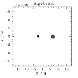
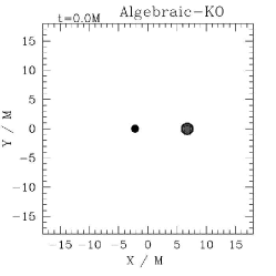
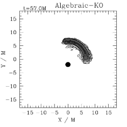
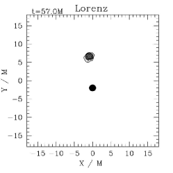
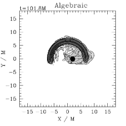
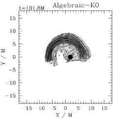
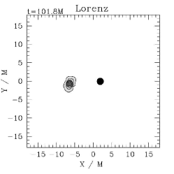
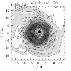
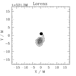
Figure 1: Snapshots of $|\mathbf{A}|$ (the magnitude of $A_{i}$) profiles in the orbital plane of a BHNS binary plotted at selected times according to $|\mathbf{A}|=10^{-3-0.6i},\ i=0,\ldots,5$, with darker greyscaling for stronger $|\mathbf{A}|$. Notice the $A_{i}$ trail left behind the orbiting NS in the algebraic gauge with or without KOD, and the absence of such trail in the Lorenz gauge. This trail is an immediate consequence of the existence of a static mode in the algebraic gauge. When the refinement boxes intersect the $A_{i}$ trail, spurious magnetic fields are generated. The filled black circled near the center denotes the BH’s horizon.

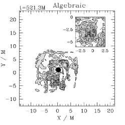
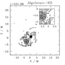
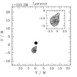
Figure 2: Orbital-plane snapshots of the comoving magnetic energy density ($b^{2}$) just before NS tidal disruption. $b^{2}$ profiles are plotted according to $b^{2}=10^{-4.49-1.4i}/M^{2},\ i=0,\ldots,5$, with darker greyscaling for larger values. The insets zoom in on the NS and demonstrate that the B-field structure is maintained in the outer layers of the NS when using Lorenz gauge, whereas it is blown away at this time when the algebraic gauge is used with or without KOD. Note also the spurious B-fields that have appeared at refinement level boundaries using the algebraic gauge. These snapshots clearly demonstrate that the algebraic gauge with or without KOD generates spurious magnetic fields and destroys the B-field structure of the NS.

V Results

V.1 Cases and grid structure

Table 1 summarizes all simulations presented here. The only parameters varied in the BHNS simulations shown here are the EM gauge condition and the application of fourth-order KOD to the $A_{i}$ evolution of the form $\epsilon/16(\Delta x^{3}\partial_{x}^{(4)}+\Delta y^{3}\partial_{y}^{(4)}+\Delta z^{3}\partial_{z}^{(4)})f$ (with strength parameter set to 0.1). Here $f$ denotes the vector potential. Note that this KOD term converges to zero at third-order in the grid spacing, so that it does not alter the convergence properties of our EM evolution scheme. One simulation adopts the Lorenz gauge without KOD (named “Lorenz”), and two simulations adopt the algebraic gauge – one with and one without KOD, called “Algebraic-KO” and “Algebraic”, respectively. The grid structure used in our simulations is presented in Table 2 and is the same for all cases. Our main findings are summarized in Figs. 1 and 2.

V.2 Algebraic gauge

Figure 1 demonstrates that in the algebraic gauge (left two columns), there is an eigenmode of the $A_{i}$-field which does not propagate (as derived in Eq. (18)) leading to a path of $A_{i}$ fields that trails the orbiting NS. Two nested sets of adaptive-mesh refinement boxes surround and comove with the NS and BH, with lower resolution at larger distances from these objects (see Table 2). When refinement levels cross the $A_{i}$ trail, the $A_{i}$ fields are filtered to lower or higher frequencies. This filtering leads to the appearance of spurious, strong magnetic fields on refinement box boundaries (see Fig. 2). When the spurious, strong magnetic fields appear, the magnetic energy outside the horizon jumps by about 5% after about half an orbit – a strong effect. Kreiss-Oliger dissipation helps to damp the spuriously generated magnetic fields, resulting in an initial net drop of magnetic energy outside the horizon by 5% after about half an orbit. Corresponding to this drop in magnetic energy, KOD gradually smooths the initially steep $A_{i}$-field gradient in the NS, ultimately destroying the NS’s magnetic field structure (inset of middle frame in Fig. 2). Just before tidal disruption the magnetic energy outside the horizon in the Algebraic and the AlgebraicKO cases is about 17% and 77% higher than the magnetic energy in the Lorenz case, respectively. Moreover, when KOD is turned on, the $b^{2}$ contours lag behind the corresponding $b^{2}$ contours when employing either the algebraic gauge without KOD or the Lorenz gauge (compare the insets in Fig. 2).

V.3 Lorenz gauge

In contrast to the algebraic gauge, there are no zero-speed modes in the Lorenz gauge (see Eq. (20)), and no $A_{i}$ field trail appears behind the NS (third-column plots in Fig. 1). Immediately after the simulation begins, an initial burst of an $A_{i}$ gauge wave (with a negligibly small $B$ field associated with it) emanates from the NS, propagates outwards and is partially absorbed by the BH. This wave travels at the speed of light, as expected for the gauge modes $\lambda_{1,2}$ in Eq. (20). As the NS orbits the BH, the $A_{i}$ field comoves with the plasma. Therefore, strong, spurious magnetic fields at refinement boundaries do not appear (right frame in Fig. 2). Also, since KOD is not used, the original magnetic field structure of the NS is better-maintained (inset of right panel in Fig. 2) than in the algebraic gauge simulations.

VI Summary

In developing an GRMHD algorithm that maintains $\mathbf{\nabla\cdot B}=0$ and is compatible with the moving puncture technique, we have focused on CT schemes. Such schemes guarantee that $\mathbf{\nabla\cdot B}=0$ is maintained to truncation error. In ELS2010 , we developed an AMR-compatible CT scheme, in which the magnetic induction equation is recast as an evolution equation for the magnetic vector potential. The divergence-free magnetic field is then computed via the curl of the vector potential. Unlike the magnetic field, the vector potential is not constrained, and so any interpolation scheme can be used during prolongation and restriction, thus enabling its use with any AMR algorithm. In addition, given that the vector potential does not uniquely determine the magnetic field, there is an extra gauge degree of freedom that can be used to one’s advantage.

In ELS2010 we performed several tests on our new AMR-compatible CT scheme. Using an algebraic EM gauge condition we found that our scheme works well even in black-hole spacetimes. Hence our scheme is compatible with the moving puncture technique. However, when we use this EM gauge condition in the evolution of magnetized binary BHNSs, stable, long-term simulations are not possible.

In this paper, we introduced a new EM gauge condition, the Lorenz gauge, which allows for stable, long-term GRMHD evolutions of binary BHNSs. Performing an eigenvalue analysis we found that static EM modes are present when adopting the algebraic gauge, whereas all modes are propagating when the Lorenz gauge is adopted.

Using magnetized BHNS simulations, we confirmed the expected behavior implied by the eigenmode analysis. As the magnetized NS orbits the BH, static modes in the algebraic gauge lead to a trail of nonzero $A_{i}$ left behind the NS. When such static modes from the algebraic gauge are interpolated at refinement boundaries, spurious B-fields are generated which remain on the grid. This spurious effect contaminates the solution and is amplified in time, forcing the simulations to terminate shortly after the NS tidal disruption. In contrast to the algebraic gauge, when the Lorenz gauge is adopted, such spurious effects are quickly propagated away to the boundary and leave the computational domain. Overall we find that the Lorenz gauge provides a major improvement over the algebraic gauge for magnetized BHNS simulations. In a forthcoming paper elpb11 we employ the Lorenz gauge to perform a detailed study of the effects of magnetic fields in the evolution of binary BHNSs.

Despite the excellent behavior observed for BHNS simulations when using the Lorenz gauge, this gauge choice may not be the optimal one for all situations. For example, we find that the algebraic gauge yields a better result in the magnetized Bondi accretion problem with radial magnetic fields. This is likely due to the fact that the system is stationary and the evolution in the algebraic gauge rigorously preserves the stationary property: $\partial_{t}A_{i}=\epsilon_{ijk}v^{j}B^{k}=0$ for radial $v^{i}$ and $B^{i}$. It is therefore useful to explore different EM gauge conditions for different problems. Alternatively, one may consider evolving $B^{i}$ directly and construct divergence-free interpolation schemes between refinement levels Balsara01 ; Balsara09 ; McNally11 , although implementation of these schemes may be less straightforward.

- (1) M. D. Duez, S. L. Shapiro, and H.-J. Yo, Phys. Rev. D 69, 104016 (May 2004)
- (2) Z. B. Etienne, Y. T. Liu, and S. L. Shapiro, Phys. Rev. D 82, 084031 (Oct. 2010), arXiv:1007.2848 [astro-ph.HE]
- (3) M. Shibata and T. Nakamura, Phys. Rev. D 52, 5428 (Nov. 1995)
- (4) T. W. Baumgarte and S. L. Shapiro, Phys. Rev. D 59, 024007 (Jan. 1998)
- (5) G. Tóth, Journal of Computational Physics 161, 605 (2000)
- (6) M. D. Duez, Y. T. Liu, S. L. Shapiro, M. Shibata, and B. C. Stephens, Physical Review Letters 96, 031101 (Jan. 2006)
- (7) M. D. Duez, Y. T. Liu, S. L. Shapiro, M. Shibata, and B. C. Stephens, Phys. Rev. D 73, 104015 (May 2006)
- (8) B. C. Stephens, S. L. Shapiro, and Y. T. Liu, Phys. Rev. D 77, 044001 (Feb 2008), http://link.aps.org/doi/10.1103/PhysRevD.77.044001
- (9) M. Shibata, Y. T. Liu, S. L. Shapiro, and B. C. Stephens, Phys. Rev. D 74, 104026 (Nov. 2006)
- (10) Y. T. Liu, S. L. Shapiro, and B. C. Stephens, Phys. Rev. D 76, 084017 (Oct. 2007)
- (11) Y. T. Liu, S. L. Shapiro, Z. B. Etienne, and K. Taniguchi, Phys. Rev. D 78, 024012 (Jul. 2008)
- (12) Z. B. Etienne, J. A. Faber, Y. T. Liu, S. L. Shapiro, K. Taniguchi, and T. W. Baumgarte, Phys. Rev. D 77, 084002 (Apr. 2008)
- (13) Z. B. Etienne, Y. T. Liu, S. L. Shapiro, and T. W. Baumgarte, Phys. Rev. D 79, 044024 (Feb. 2009)
- (14) V. Paschalidis, Z. Etienne, Y. T. Liu, and S. L. Shapiro, Phys. Rev. D 83, 064002 (Mar. 2011), arXiv:1009.4932 [astro-ph.HE]
- (15) V. Paschalidis, Y. T. Liu, Z. Etienne, and S. L. Shapiro, ArXiv e-prints(Sep. 2011), arXiv:1109.5177 [astro-ph.HE]
- (16) B. D. Farris, Y. T. Liu, and S. L. Shapiro, Phys. Rev. D 81, 084008 (Apr. 2010), arXiv:0912.2096 [astro-ph.HE]
- (17) B. D. Farris, Y. T. Liu, and S. L. Shapiro, Phys. Rev. D 84, 024024 (Jul. 2011), arXiv:1105.2821 [astro-ph.HE]
- (18) J. U. Brackbill and D. C. Barnes, Journal of Computational Physics 35, 426 (1980)
- (19) D. S. Balsara and D. S. Spicer, Journal of Computational Physics 149, 270 (1999)
- (20) C. R. Evans and J. F. Hawley, Astrophys. J. 332, 659 (Sep. 1988)
- (21) A. Dedner, F. Kemm, D. Kröner, C. Munz, T. Schnitzer, and M. Wesenberg, Journal of Computational Physics 175, 645 (2002)
- (22) M. Anderson, E. W. Hirschmann, S. L. Liebling, and D. Neilsen, Classical and Quantum Gravity 23, 6503 (Nov. 2006), arXiv:gr-qc/0605102
- (23) M. Campanelli, C. O. Lousto, P. Marronetti, and Y. Zlochower, Phys. Rev. Lett. 96, 111101 (Mar. 2006)
- (24) J. G. Baker, J. Centrella, D.-I. Choi, M. Koppitz, and J. van Meter, Phys. Rev. Lett. 96, 111102 (Mar. 2006)
- (25) J. D. Brown, Phys. Rev. D 80, 084042 (Oct 2009), http://link.aps.org/doi/10.1103/PhysRevD.80.084042
- (26) Z. B. Etienne, J. A. Faber, Y. T. Liu, S. L. Shapiro, and T. W. Baumgarte, Phys. Rev. D 76, 101503(R) (Nov. 2007)
- (27) D. Brown, O. Sarbach, E. Schnetter, M. Tiglio, P. Diener, I. Hawke, and D. Pollney, Phys. Rev. D 76, 081503 (Oct. 2007)
- (28) D. Brown, P. Diener, O. Sarbach, E. Schnetter, and M. Tiglio, ArXiv e-prints(Sep. 2008), arXiv:0809.3533
- (29) D. S. Balsara, Journal of Computational Physics 174, 614 (2001)
- (30) D. S. Balsara, Journal of Computational Physics 228, 5040 (2009)
- (31) C. P. McNally, Month. Not. Roy. Astron. Soc. 413, L76 (May 2011), arXiv:1102.4852 [astro-ph.IM]
- (32) L. Del Zanna, N. Bucciantini, and P. Londrillo, Astron. and Astrophys. 400, 397 (Mar. 2003)
- (33) B. Giacomazzo, L. Rezzolla, and L. Baiotti, Phys. Rev. D 83, 044014 (Feb 2011)
- (34) Note that the EM Lorenz gauge condition is named after Ludvig Lorenz and not after Hendrik Lorentz known for the Lorentz transformations (see also note in p. 294 in Jackson3rd ).
- (35) Z. B. Etienne, Y. T. Liu, V. Paschalidis, and S. L. Shapiro, ArXiv e-prints(Dec. 2011), arXiv:1112.0568 [astro-ph.HE]
- (36) T. W. L. Baumgarte and S. L. Shapiro, Numerical Relativity (Cambridge University Press, 2010)
- (37) J. R. van Meter, J. G. Baker, M. Koppitz, and D.-I. Choi, Phys. Rev. D 73, 124011 (Jun. 2006)
- (38) T. W. Baumgarte and S. L. Shapiro, Astrophys. J. 585, 921 (Mar. 2003)
- (39) B. Gustafsson, H.-O. Kreiss, and J. Oliger, Time dependent problems and difference methods (John Willey & Sons, New York, 1995)
- (40) H.-O. Kreiss and J. Lorenz, Initial-Boundary Value Problems and the Navier-Stokes Equations (Academic Press Inc., 1989)
- (41) Strictly speaking, for the quasi-linear, partial differential equations considered here, the existence of real eigenvalues and a complete set of eigenvectors are only necessary conditions for strong hyperbolicity (see GKOpdeBook ; KLpdeBook for complete definitions of strong hyperbolicity). However, here we are not interested in rigorously proving strong hyperbolicity. We are only interested in identifying the eigenvalues of the characteristic matrix and, in particular, whether static modes exist or not.
- (42) M. Alcubierre, G. Allen, B. Brügmann, E. Seidel, and W.-M. Suen, Phys. Rev. D 62, 124011 (Dec. 2000), arXiv:gr-qc/9908079
- (43) H.-a. Shinkai and G. Yoneda, ArXiv General Relativity and Quantum Cosmology e-prints(Sep. 2002), arXiv:gr-qc/0209111
- (44) V. Paschalidis, Phys. Rev. D 78, 024002 (Jul. 2008), arXiv:0704.2861 [gr-qc]
- (45) V. Paschalidis, J. Hansen, and A. Khokhlov, Phys. Rev. D 78, 064048 (Sep. 2008), arXiv:0712.1258 [gr-qc]
- (46) K. Taniguchi, T. W. Baumgarte, J. A. Faber, and S. L. Shapiro, Phys. Rev. D 77, 044003 (Feb. 2008)
- (47) J.-P. De Villiers, J. F. Hawley, and J. H. Krolik, Astrophys. J. 599, 1238 (Dec. 2003)
- (48) J. C. McKinney and C. F. Gammie, Astrophys. J. 611, 977 (Aug. 2004)
- (49) M. Anderson, E. W. Hirschmann, L. Lehner, S. L. Liebling, P. M. Motl, D. Neilsen, C. Palenzuela, and J. E. Tohline, Phys. Rev. Lett. 100, 191101 (May 2008)
- (50) S. Chawla, M. Anderson, M. Besselman, L. Lehner, S. L. Liebling, P. M. Motl, and D. Neilsen, Physical Review Letters 105, 111101 (Sep. 2010)
- (51) S. C. Noble, C. F. Gammie, J. C. McKinney, and L. Del Zanna, Astrophys. J. 641, 626 (Apr. 2006)
- (52) S. C. Noble, C. F. Gammie, J. C. McKinney, and L. Del Zanna(2006), publicly available on http://rainman.astro.illinois.edu/codelib/
- (53) K. Beckwith and J. M. Stone, Astrophys. J. Supp. 193, 6 (Mar. 2011)
- (54) J. D. Jackson, Classical Electrodynamics, 3rd Edition, by John David Jackson, ISBN 0-471-30932-X. Wiley-VCH , July 1998. (1998)