Merger of binary neutron stars with realistic equations of state in full general relativity

Abstract

We present numerical results of three-dimensional simulations for the merger of binary neutron stars in full general relativity. Hybrid equations of state are adopted to mimic realistic nuclear equations of state. In this approach, we divide the equations of state into two parts as $P=P_{\rm cold}+P_{\rm th}$. $P_{\rm cold}$ is the cold part for which we assign a fitting formula for realistic equations of state of cold nuclear matter slightly modifying the formula developed by Haensel and Potekhin. We adopt the SLy and FPS equations of state for which the maximum allowed ADM mass of cold and spherical neutron stars is $\approx 2.04M_{\odot}$ and $1.80M_{\odot}$, respectively. $P_{\rm th}$ denotes the thermal part which is written as $P_{\rm th}=(\Gamma_{\rm th}-1)\rho(\varepsilon-\varepsilon_{\rm cold})$, where $\rho$, $\varepsilon$, $\varepsilon_{\rm cold}$, and $\Gamma_{\rm th}$ are the baryon rest-mass density, total specific internal energy, specific internal energy of the cold part, and the adiabatic constant, respectively. Simulations are performed for binary neutron stars of the total ADM mass in the range between $2.4M_{\odot}$ and $2.8M_{\odot}$ with the rest-mass ratio $Q_{M}$ to be in the range $0.9\mathrel{\raise 1.29167pt\hbox{$<$}\mkern-14.0mu\lower 2.58334pt\hbox{$\sim$}}Q_{M}\leq 1$. It is found that if the total ADM mass of the system is larger than a threshold $M_{\rm thr}$, a black hole is promptly formed in the merger irrespective of the mass ratios. In the other case, the outcome is a hypermassive neutron star of a large ellipticity, which results from the large adiabatic index of the realistic equations of state adopted. The value of $M_{\rm thr}$ depends on the equation of state: $M_{\rm thr}\sim 2.7M_{\odot}$ and $\sim 2.5M_{\odot}$ for the SLy and FPS equations of state, respectively. Gravitational waves are computed in terms of a gauge-invariant wave extraction technique. In the formation of the hypermassive neutron star, quasiperiodic gravitational waves of a large amplitude and of frequency between 3 and 4 kHz are emitted. The estimated emission time scale is $\mathrel{\raise 1.29167pt\hbox{$<$}\mkern-14.0mu\lower 2.58334pt\hbox{$\sim$}}100$ ms, after which the hypermassive neutron star collapses to a black hole. Because of the long emission time, the effective amplitude may be large enough to be detected by advanced laser interferometric gravitational wave detectors if the distance to the source is smaller than $\sim 100$ Mpc. Thermal properties of the outcome formed after the merger are also analyzed to approximately estimate the neutrino emission energy.

I Introduction

Binary neutron stars HT ; Stairs inspiral as a result of the radiation reaction of gravitational waves, and eventually merge. The most optimistic scenario based mainly on a recent discovery of binary system PSRJ0737-3039 NEW suggests that such mergers may occur approximately once per year within a distance of about 50 Mpc BNST . Even the most conservative scenario predicts an event rate approximately once per year within a distance of about 100 Mpc BNST . This indicates that the detection rate of gravitational waves by the advanced LIGO will be $\sim 40$–600 yr^-1. Thus, the merger of binary neutron stars is one of the most promising sources for kilometer-size laser interferometric detectors KIP ; Ando .

Hydrodynamic simulations employing full general relativity provide the best approach for studying the merger of binary neutron stars. Over the last few years, numerical methods for solving coupled equations of the Einstein and hydrodynamic equations have been developed gr3d ; bina ; bina2 ; other ; Font ; STU ; marks ; illinois ; Baiotti and now such simulations are feasible with an accuracy high enough for yielding scientific results STU . With the current implementation, radiation reaction of gravitational waves in the merger of binary neutron stars can be taken into account within $\sim 1\%$ error in an appropriate computational setting STU . This fact illustrates that it is now a robust tool for the detailed theoretical study of astrophysical phenomena and gravitational waves emitted.

So far, all the simulations for the merger of binary neutron stars in full general relativity have been performed adopting an ideal equation of state bina ; bina2 ; STU ; marks ; illinois . (But, see OUPT for a simulation in an approximately general relativistic gravity.) For making better models of the merger which can be used for quantitative comparison with observational data, it is necessary to adopt more realistic equations of state as the next step. Since the lifetime (from the birth to the merger) of observed binary neutron stars is longer than $\sim 100$ million yrs Stairs , the thermal energy per nucleon in each neutron star will be much lower than the Fermi energy of neutrons ST ; Tsuruta at the onset of the merger. This implies that for modeling the binary neutron stars just before the merger, it is appropriate to use cold nuclear equations of state. During the merger, shocks will be formed and the kinetic energy will be converted to the thermal energy. However, previous studies have indicated that the shocks are not very strong in the merger of binary neutron stars, in contrast to those in iron core collapse of massive stars. The reason is that the approaching velocity at the first contact of two neutron stars is much smaller than the orbital velocity and the sound speed of nuclear matter (e.g., STU ). This implies that the pressure and the internal energy associated with the finite thermal energy (temperature) are not still as large as those of the cold part. From this reason, we adopt a hybrid equation of state in which the finite-temperature part generated by shocks is added as a correction using a simple prescription (see Sec. II B). On the other hand, realistic equations of state are assigned to the cold part PR ; DH ; HP .

The motivation which stimulates us to perform new simulations is that the stiffness and adiabatic index of the realistic equations of state are quite different from those in the $\Gamma$-law equation of state with $\Gamma=2$ (hereafter referred to as the $\Gamma=2$ equation of state) which has been widely adopted so far (e.g., STU ) . It can be expected that these differences will modify the properties of the merger quantitatively as described in the following.

Since the realistic equations of state are softer than the $\Gamma=2$ one, each neutron star becomes more compact (cf. Fig. 2). This implies that the merger will set in at a more compact state which is reached after more energy and angular momentum are already dissipated by gravitational radiation. Namely, compactness of the system at the onset of the merger is larger. This will modify the dynamics of the merger, and accordingly, the threshold mass for prompt black hole formation (hereafter $M_{\rm thr}$) will be changed.

The adiabatic index of the equations of state is also different from that for the $\Gamma=2$ equation of state. This will modify the shape of the hypermassive neutron stars , which are formed after the merger in the case that the total mass is smaller than $M_{\rm thr}$. Previous Newtonian and post Newtonian studies RS ; C ; FR have indicated that for smaller adiabatic index of the equations of state, the degree of the nonaxial symmetry of the formed neutron star becomes smaller. However, if its value is sufficiently large, the formed neutron star can be ellipsoidal. As a result of this change, the amplitude of gravitational waves emitted from the formed neutron star is significantly changed. Since the adiabatic index of the realistic equations of state is much larger than that of the $\Gamma=2$ equation of state for supranuclear density PR ; DH ; HP , the significant modification in the shape of the hypermassive neutron stars and in the amplitude of gravitational waves emitted from them is expected.

The paper is organized as follows. In Sec. II A–C, basic equations, gauge conditions, methods for extracting gravitational waves, and quantities used in the analysis for numerical results are reviewed. Then, the hybrid equations of state adopted in this paper are described in Sec. II D. In Sec. III, after briefly describing the computational setting and the method for computation of initial condition, the numerical results are presented. We pay particular attention to the merger process, the outcome, and gravitational waveforms. Section IV is devoted to a summary. Throughout this paper, we adopt the geometrical units in which $G=c=1$ where $G$ and $c$ are the gravitational constant and the speed of light. Latin and Greek indices denote spatial components ($x,y,z$) and space-time components ($t,x,y,z$), respectively: $r\equiv\sqrt{x^{2}+y^{2}+z^{2}}$. $\delta_{ij}(=\delta^{ij})$ denotes the Kronecker delta.

II Formulation

II.1 Summary of formulation

Our formulation and numerical scheme for fully general relativistic simulations in three spatial dimensions are the same as in STU , to which the reader may refer for details of basic equations and successful numerical results.

The fundamental variables for the hydrodynamics are $\rho$: rest-mass density, $\varepsilon$ : specific internal energy, $P$ : pressure, $u^{\mu}$ : four velocity, and

$$v^{i}={dx^{i}\over dt}={u^{i}\over u^{t}},$$ (1)

where subscripts $i,j,k,\cdots$ denote $x,y$ and $z$, and $\mu$ the spacetime components. The fundamental variables for geometry are $\alpha$: lapse function, $\beta^{k}$: shift vector, $\gamma_{ij}$: metric in three-dimensional spatial hypersurface, $\gamma\equiv e^{12\phi}={\rm det}(\gamma_{ij})$, $\tilde{\gamma}_{ij}=e^{-4\phi}\gamma_{ij}$: conformal three-metric, and $K_{ij}$: extrinsic curvature.

For a numerical implementation of the hydrodynamic equations, we define a weighted density, a weighted four-velocity, and a specific energy defined, respectively, by

$$\rho_{*}\equiv\rho\alpha u^{t}e^{6\phi},$$ (2)

$$\hat{u}_{i}\equiv hu_{i},$$ (3)

$$\hat{e}\equiv h\alpha u^{t}-{P\over\rho\alpha u^{t}},$$ (4)

where $h=1+\varepsilon+P/\rho$ denotes the specific enthalpy. General relativistic hydrodynamic equations are written into the conservative form for variables $\rho_{*}$, $\rho_{*}\hat{u}_{i}$, and $\rho_{*}\hat{e}$, and solved using a high-resolution shock-capturing scheme Font . In our approach, the transport terms such as $\partial_{i}(\cdots)$ are computed by an approximate Riemann solver with third-order (piecewise parabolic) spatial interpolation with a Roe-type averaging shiba2d . At each time step, $\alpha u^{t}$ is determined by solving an algebraic equation derived from the normalization $u^{\mu}u_{\mu}=-1$, and then, the primitive variables such as $\rho$, $\epsilon$, and $v^{i}$ are updated. An atmosphere of small density $\rho\sim 10^{9}~{}{\rm g/cm^{3}}$ is added uniformly outside neutron stars at $t=0$, since the vacuum is not allowed in the shock-capturing scheme. The integrated mass of the atmosphere is at most $1\%$ of the total mass in the present simulation. Furthermore, we add a friction term for a matter of low density $\sim 10^{9}~{}{\rm g/cm^{3}}$ to avoid infall of such atmosphere toward the central region. Hence, the effect of the atmosphere for the evolution of binary neutron stars is very small.

The Einstein evolution equations are solved using a version of the BSSN formalism following previous papers SN ; gr3d ; bina2 ; STU : We evolve $\tilde{\gamma}_{ij}$, $\phi$, $\tilde{A}_{ij}\equiv e^{-4\phi}(K_{ij}-\gamma_{ij}K_{k}^{~{}k})$, and the trace of the extrinsic curvature $K_{k}^{~{}k}$ together with three auxiliary functions $F_{i}\equiv\delta^{jk}\partial_{j}\tilde{\gamma}_{ik}$ using an unconstrained free evolution code. The latest version of our formulation and numerical method is described in STU . The point worthy to note is that the equation for $\phi$ is written to a conservative form similar to the continuity equation, and solving this improves the accuracy of the conservation of the ADM mass and angular momentum significantly.

As the time slicing condition, an approximate maximal slice (AMS) condition $K_{k}^{~{}k}\approx 0$ is adopted following previous papers bina2 . As the spatial gauge condition, we adopt a hyperbolic gauge condition as in S03 ; STU . Successful numerical results for the merger of binary neutron stars in these gauge conditions are presented in STU . In the presence of a black hole, the location is determined using an apparent horizon finder for which the method is described in AH .

Following previous works, we adopt binary neutron stars in quasiequilibrium circular orbits as the initial condition. In computing the quasiequilibrium state, we use the so-called conformally flat formalism for the Einstein equation WM . A solution in this formalism satisfies the constraint equations in general relativity, and hence, it can be used for the initial condition. The irrotational velocity field is assumed since it is considered to be a good approximation for coalescing binary neutron stars in nature CBS . The coupled equations of the field and hydrostatic equations irre are solved by a pseudospectral method developed by Bonazzola, Gourgoulhon, and Marck GBM . Detailed numerical calculations have been done by Taniguchi and part of the numerical results are presented in TG .

II.2 Extracting gravitational waves

Gravitational waves are computed in terms of the gauge-invariant Moncrief variables in a flat spacetime moncrief as we have been carried out in our series of paper (e.g., gw3p2 ; STU ; SS3 ). The detailed equations are describe in STU ; SS3 to which the reader may refer. In this method, we split the metric in the wave zone into the flat background and linear perturbation. Then, the linear part is decomposed using the tensor spherical harmonics and gauge-invariant variables are constructed for each mode of eigen values $(l,m)$. The gauge-invariant variables of $l\geq 2$ can be regarded as gravitational waves in the wave zone, and hence, we focus on such mode. In the merger of binary neutron stars of nearly equal mass, the even-parity mode of $(l,|m|)=(2,2)$ is much larger than other modes. Thus, in the following, we pay attention only to this mode.

Using the gauge-invariant variables, the luminosity and the angular momentum flux of gravitational waves can be defined by

$${dE\over dt}={r^{2}\over 32\pi}\sum_{l,m}\Bigl{[}|\partial_{t}R_{lm}^{\rm E}|^{2}+|\partial_{t}R_{lm}^{\rm O}|^{2}\Bigr{]},$$ (5)

$${dJ\over dt}={r^{2}\over 32\pi}\sum_{l,m}\Bigl{[}|m(\partial_{t}R_{lm}^{\rm E})R_{lm}^{\rm E}|+|m(\partial_{t}R_{lm}^{\rm O})R_{lm}^{\rm O}|\Bigr{]},$$ (6)

where $R_{lm}^{\rm E}$ and $R_{lm}^{\rm O}$ are the gauge-invariant variables of even and odd parities. The total radiated energy and angular momentum are obtained by the time integration of $dE/dt$ and $dJ/dt$.

To search for the characteristic frequencies of gravitational waves, the Fourier spectra are computed by

$$\bar{R}_{lm}(f)=\int e^{2\pi ift}R_{lm}(t)dt,$$ (7)

where $f$ denotes a frequency of gravitational waves. Using the Fourier spectrum, the energy power spectrum is defined as

$${dE\over df}={\pi\over 4}r^{2}\sum_{l\geq 2,m\geq 0}|\bar{R}_{lm}(f)f|^{2}~{}~{}~{}(f>0),$$ (8)

where for $m\not=0$, we define

$$\bar{R}_{lm}(f)\equiv\sqrt{|\bar{R}_{lm}(f)|^{2}+|\bar{R}_{l-m}(f)|^{2}}~{}~{}(m>0),$$ (9)

and use $|\bar{R}_{lm}(-f)|=|\bar{R}_{lm}(f)|$ for deriving Eq. (8).

We also use a quadrupole formula which is described in SS1 ; SS2 ; SS3 . As shown in SS1 , a kind of quadrupole formula can provide approximate gravitational waveforms from oscillating compact stars. In this paper, the applicability is tested for the merger of binary neutron stars.

In quadrupole formulas, gravitational waves are computed from

$$h_{ij}=\biggl{[}P_{i}^{~{}k}P_{j}^{~{}l}-{1\over 2}P_{ij}P^{kl}\biggr{]}\biggl{(}{2\over r}{d^{2}\hbox{$\,I\!\!\!$--}_{kl}\over dt^{2}}\biggr{)},$$ (10)

where $\hbox{$\,I\!\!\!$--}_{ij}$ and $P_{ij}=\delta_{ij}-n_{i}n_{j}$ ($n_{i}=x^{i}/r$) denote a tracefree quadrupole moment and a projection tensor.

In fully general relativistic and dynamical spacetimes, there is no unique definition for the quadrupole moment $I_{ij}$. Following SS1 ; SS2 ; SS3 , we choose the formula as

$$I_{ij}=\int\rho_{*}x^{i}x^{j}d^{3}x.$$ (11)

Then, using the continuity equation, the first time derivative is computed as

$$\dot{I}_{ij}=\int\rho_{*}(v^{i}x^{j}+x^{i}v^{j})d^{3}x.$$ (12)

To compute $\ddot{I}_{ij}$, we carry out the finite differencing of the numerical result for $\dot{I}_{ij}$.

In this paper, we focus only on $l=2$ mass quadrupole modes. Then, the gravitational waveforms are written as

$$h_{+}={1\over r}\biggl{[}\sqrt{{5\over 64\pi}}\{R_{22+}(1+\cos^{2}\theta)\cos(2\varphi)$$

$$~{}~{}~{}~{}~{}~{}~{}~{}~{}~{}~{}~{}~{}~{}~{}~{}~{}~{}+R_{22-}(1+\cos^{2}\theta)\sin(2\varphi)\}$$

$$~{}~{}~{}~{}~{}~{}~{}~{}~{}~{}+\sqrt{{15\over 64\pi}}R_{20}\sin^{2}\theta\biggr{]},$$ (13)

$$h_{\times}={2\over r}\sqrt{{5\over 64\pi}}\Bigl{[}-R_{22+}\cos\theta\sin(2\varphi)$$

$$~{}~{}~{}~{}~{}~{}~{}~{}~{}~{}~{}~{}~{}~{}~{}~{}~{}~{}~{}+R_{22-}\cos\theta\cos(2\varphi)\Bigr{]},$$ (14)

in the gauge-invariant wave extraction technique, and

$$h_{+}={1\over r}\biggl{[}{\ddot{I}_{xx}-\ddot{I}_{yy}\over 2}(1+\cos^{2}\theta)\cos(2\varphi)$$

$$~{}~{}~{}~{}~{}~{}~{}~{}~{}~{}~{}+\ddot{I}_{xy}(1+\cos^{2}\theta)\sin(2\varphi)$$

$$~{}~{}~{}~{}~{}~{}~{}~{}~{}~{}~{}+\biggl{(}\ddot{I}_{zz}-{\ddot{I}_{xx}+\ddot{I}_{yy}\over 2}\biggr{)}\sin^{2}\theta\biggr{]},$$ (15)

$$h_{\times}={2\over r}\biggl{[}-{\ddot{I}_{xx}-\ddot{I}_{yy}\over 2}\cos\theta\sin(2\varphi)$$

$$~{}~{}~{}~{}~{}~{}~{}~{}~{}~{}~{}~{}~{}+\ddot{I}_{xy}\cos\theta\cos(2\varphi)\biggr{]},$$ (16)

in the quadrupole formula. In Eqs. (13) and (14), we use the variables defined by

$$R_{22\pm}\equiv{R_{22}^{\rm E}\pm R_{2~{}-2}^{\rm E}\over\sqrt{2}}r,$$ (17)

$$R_{20}\equiv R_{20}^{\rm E}r.$$ (18)

For the derivation of $h_{+}$ and $h_{\times}$, we assume that the wave part of the spatial metric in the wave zone is written as

$$dl^{2} =dr^{2}+r^{2}[(1+h_{+})d\theta^{2}+\sin^{2}\theta(1-h_{+})d\varphi^{2}$$ (19)

$$~{}~{}~{}~{}~{}~{}~{}~{}~{}~{}~{}~{}~{}+2\sin\theta h_{\times}d\theta d\varphi],$$

and set $R_{2~{}\pm 1}^{\rm E}=0$ and $I_{xz}=I_{yz}=0$ since we assume the reflection symmetry with respect to the equatorial plane.

In the following, we present

$$R_{+}=\sqrt{{5\over 16\pi}}R_{22+},$$ (20)

$$R_{\times}=\sqrt{{5\over 16\pi}}R_{22-},$$ (21)

in the gauge-invariant wave extraction method, and as the corresponding variables,

$$A_{+}=\ddot{I}_{xx}-\ddot{I}_{yy},$$ (22)

$$A_{\times}=2\ddot{I}_{xy},$$ (23)

in the quadrupole formula. These have the unit of length and provide the amplitude of a given mode measured by an observer located in the most optimistic direction.

II.3 Definitions of quantities and methods for calibration

In numerical simulations, we refer to the total baryon rest-mass, the ADM mass, and the angular momentum of the system, which are given by

$$M_{*} \equiv\int\rho_{*}d^{3}x,$$ (24)

$$M \equiv-{1\over 2\pi}\oint_{r\rightarrow\infty}\partial_{i}\psi dS_{i}$$ (25)

$$=\int\biggl{[}\rho_{\rm H}e^{5\phi}+{e^{5\phi}\over 16\pi}\biggl{(}\tilde{A}_{ij}\tilde{A}^{ij}-{2\over 3}(K_{k}^{~{}k})^{2}$$

$$~{}~{}~{}~{}~{}~{}~{}~{}~{}~{}~{}~{}~{}~{}~{}~{}~{}~{}~{}~{}~{}~{}~{}~{}~{}~{}~{}~{}~{}~{}-\tilde{R}_{k}^{~{}k}e^{-4\phi}\biggr{)}\biggr{]}d^{3}x,$$

$$J \equiv{1\over 8\pi}\oint_{r\rightarrow\infty}\varphi^{i}\tilde{A}_{i}^{~{}j}e^{6\phi}dS_{j}$$ (26)

$$=\int e^{6\phi}\biggl{[}J_{i}\varphi^{i}+{1\over 8\pi}\biggl{(}\tilde{A}_{i}^{~{}j}\partial_{j}\varphi^{i}-{1\over 2}\tilde{A}_{ij}\varphi^{k}\partial_{k}\tilde{\gamma}^{ij}$$

$$~{}~{}~{}~{}~{}~{}~{}~{}~{}~{}~{}~{}~{}~{}~{}~{}~{}~{}~{}~{}~{}~{}~{}~{}~{}~{}+{2\over 3}\varphi^{j}\partial_{j}K_{k}^{~{}k}\biggr{)}\biggr{]}d^{3}x,$$

where $dS_{j}=r^{2}\partial_{j}rd(\cos\theta)d\varphi$, $\varphi^{j}=-y(\partial_{x})^{j}+x(\partial_{y})^{j}$, $\psi=e^{\phi}$, $\rho_{\rm H}=\rho\alpha u^{t}\hat{e}$, $J_{i}=\rho\hat{u}_{i}$, and $\tilde{R}_{k}^{~{}k}$ denotes the Ricci scalar with respect to $\tilde{\gamma}_{ij}$. To derive the expressions for $M$ and $J$ in the form of volume integral, the Gauss law is used. Here, $M_{*}$ is a conserved quantity. We also use the notations $M_{*1}$ and $M_{*2}$ which denote the baryon rest-mass of the primary and secondary neutron stars, respectively. In terms of them, the baryon rest-mass ratio is defined by $Q_{M}=M_{*2}/M_{*1}(\leq 1)$.

In numerical simulation, $M$ and $J$ are computed using the volume integral shown in Eqs. (25) and (26). Since the computational domain is finite, they are not constant and decrease after gravitational waves propagate to the outside of the computational domain during time evolution. Therefore, in the following, they are referred to as the ADM mass and the angular momentum computed in the finite domain (or simply as $M$ and $J$, which decrease with time).

The decrease rates of $M$ and $J$ should be equal to the emission rates of the energy and the angular momentum by gravitational radiation according to the conservation law. Denoting the radiated energy and angular momentum from the beginning of the simulation to the time $t$ as $\Delta E(t)$ and $\Delta J(t)$, the conservation relations are written as

$$M(t)+\Delta E(t)=M_{0},$$ (27)

$$J(t)+\Delta J(t)=J_{0},$$ (28)

where $M_{0}$ and $J_{0}$ are the initial values of $M$ and $J$. We check if these conservation laws hold during the simulation.

Significant violation of the conservation laws indicates that the radiation reaction of gravitational waves is not taken into account accurately. During the merger of binary neutron stars, the angular momentum is dissipated by several $10\%$, and thus, the dissipation effect plays an important role in the evolution of the system. Therefore, it is required to confirm that the radiation reaction is computed accurately.

The violation of the Hamiltonian constraint is locally measured by the equation as

$$\displaystyle f_{\psi} \equiv\Bigl{|}\tilde{\Delta}\psi-{\psi\over 8}\tilde{R}_{k}^{~{}k}+2\pi\rho_{\rm H}\psi^{5}$$ (29)

$$~{}~{}~{}~{}~{}~{}~{}~{}~{}+{\psi^{5}\over 8}\Bigl{(}\tilde{A}_{ij}\tilde{A}^{ij}-{2\over 3}(K_{k}^{~{}k})^{2}\Bigr{)}\Bigr{|}$$

$$~{}~{}~{}\biggl{[}|\tilde{\Delta}\psi|+|{\psi\over 8}\tilde{R}_{k}^{~{}k}|+|2\pi\rho_{\rm H}\psi^{5}|$$

$$~{}~{}~{}~{}~{}~{}~{}~{}~{}+{\psi^{5}\over 8}\Bigl{(}|\tilde{A}_{ij}\tilde{A}^{ij}|+{2\over 3}(K_{k}^{~{}k})^{2}\Bigr{)}\biggr{]}^{-1}.$$

Following shiba2d , we define and monitor a global quantity as

$$H\equiv{1\over M_{*}}\int\rho_{*}f_{\psi}d^{3}x.$$ (30)

Hereafter, this quantity will be referred to as the averaged violation of the Hamiltonian constraint.

II.4 Equations of state

Since the lifetime of binary neutron stars from the birth to the merger is longer than $\sim 100$ million yrs for the observed systems Stairs , the temperature of each neutron star will be very low ($\mathrel{\raise 1.29167pt\hbox{$<$}\mkern-14.0mu\lower 2.58334pt\hbox{$\sim$}}10^{5}$ K) ST ; Tsuruta at the onset of merger; i.e., the thermal energy per nucleon is much smaller than the Fermi energy of neutrons. This implies that for modeling the binary neutron stars just before the merger, it is appropriate to use cold nuclear equations of state. On the other hand, during the merger, shocks will be formed and the kinetic energy will be converted to the thermal energy to increase the temperature. However, previous studies have indicated that the shocks in the merger are not strong enough to increase the thermal energy to the level as large as the Fermi energy of neutrons, since the approaching velocity at the first contact of two neutron stars is much smaller than the orbital velocity and the sound speed of nuclear matter. This implies that the pressure and the internal energy associated with the finite temperature are not still as large as those of the cold part. From this reason, we adopt a hybrid equation of state.

	$i$	$p_{i}$ (SLy)	$p_{i}$ (FPS)	$i$	$p_{i}$ (SLy)	$p_{i}$ (FPS)
	1	0.1037	0.15806	9	$9\times 10^{5}$	$9\times 10^{5}$
	2	0.1956	0.220	10	4	5
	3	39264	5956.4	11	0.75	0.75
	4	1.9503	1.633	12	0.057	0.0627
	5	254.83	170.68	13	0.138	0.1387
	6	1.3823	1.1056	14	0.84	0.56
	7	$-1.234$	$-0.703$	15	0.338	0.308
	8	$1.2\times 10^{5}$	$2\times 10^{4}$

Table 1: The values of $p_{i}$ we choose in units of $c=G=M_{\odot}=1$.

In this equation of state, we write the pressure and the specific internal energy in the form

$$P=P_{\rm cold}+P_{\rm th},$$ (31)

$$\varepsilon=\varepsilon_{\rm cold}+\varepsilon_{\rm th},$$ (32)

where $P_{\rm cold}$ and $\varepsilon_{\rm cold}$ are the cold (zero-temperature) parts, and are written as functions of $\rho$. $P_{\rm th}$ and $\varepsilon_{\rm th}$ are the thermal (finite-temperature) parts. During the simulation, $\rho$ and $\varepsilon$ are computed from hydrodynamic variables $\rho_{*}$ and $\hat{e}$. Thus, $\varepsilon_{\rm th}$ is determined by $\varepsilon-\varepsilon_{\rm cold}$.

For the cold parts, we assign realistic equations of state for zero-temperature nuclear matter. In this paper, we adopt the SLy DH and FPS equations of state PR . These are tabulated as functions of the baryon rest-mass density for a wide density range from $\sim 10~{}{\rm g/cm^{3}}$ to $\sim 10^{16}~{}{\rm g/cm^{3}}$. To simplify numerical implementation for simulation, we make fitting formulae from the tables of equations of state, slightly modifying the original approach proposed in HP .

In our approach, we first make a fitting formula for $\varepsilon_{\rm cold}$ as

$$\varepsilon_{\rm cold}(\rho)=[(1+p_{1}\rho^{p_{2}}+p_{3}\rho^{p_{4}})(1+p_{5}\rho^{p_{6}})^{p_{7}}-1]$$

$$~{}~{}~{}~{}~{}~{}~{}~{}~{}~{}~{}~{}~{}\times f(-p_{8}\rho+p_{10})$$

$$~{}~{}~{}~{}~{}~{}~{}~{}~{}~{}~{}~{}~{}+p_{12}\rho^{p_{13}}f(p_{8}\rho-p_{10})f(-p_{9}\rho+p_{11})$$

$$~{}~{}~{}~{}~{}~{}~{}~{}~{}~{}~{}~{}~{}+p_{14}\rho^{p_{15}}f(p_{9}\rho-p_{11}),$$ (33)

where

$$f(x)={1\over e^{x}+1}.$$ (34)

The coefficients $p_{i}~{}(i=$1–15) denote constants, and are listed in Table I. In making the formula, we focus only on the density for $\rho\geq 10^{10}~{}{\rm g/cm^{3}}$ in this work, since the matter of lower density does not play an important role in the merger. Then, the pressure is computed from the thermodynamic relation in the zero-temperature limit

$$P_{\rm cold}=\rho^{2}{d\varepsilon_{\rm cold}\over d\rho}.$$ (35)

With this approach, the accuracy of the fitting for the pressure is not as good as that in HP . However, the first law of the thermodynamics is completely satisfied in contrast to that in HP .

(a)   (b)

Figure 1: Pressure and specific internal energy as functions of baryon rest-mass density $\rho$ (a) for the SLy and (b) for the FPS equations of state. The solid and dotted curves denote the results by fitting formulae and numerical data tabulated, respectively.

In Fig. 1, we compare $P_{\rm cold}$ and $\varepsilon_{\rm cold}$ calculated by the fitting formulae (solid curves) with the numerical data tabulated (dotted curves) . It is found that two results agree approximately. The relative error between two is within $\sim 10\%$ for $\rho>10^{10}~{}{\rm g/cm^{3}}$ and $\mathrel{\raise 1.29167pt\hbox{$<$}\mkern-14.0mu\lower 2.58334pt\hbox{$\sim$}}2\%$ for supranuclear density with $\rho\mathrel{\raise 1.29167pt\hbox{$>$}\mkern-14.0mu\lower 2.58334pt\hbox{$\sim$}}2\times 10^{14}~{}{\rm g/cm^{3}}$.

(a)   (b)

Figure 2: (a) ADM mass (solid curves) and total baryon rest-mass (dotted curves) as functions of central baryon rest-mass density $\rho_{c}$ and (b) relation between the circumferential radius and the ADM mass for cold and spherical neutron stars in equilibrium. ’FPS’ and ’SLy’ denote the sequences for the FPS and SLy equations of state, respectively. The relations for the $\Gamma=2$ polytropic equation of state with $K_{\rm p}=1.6\times 10^{5}$ in the cgs unit are also drawn by the dashed curves.

In Fig. 2, we show the relations among the ADM mass $M$, the total baryon rest-mass $M_{*}$, the central density $\rho_{c}$, and the circumferential radius $R$ for cold and spherical neutron stars in the SLy and FPS equations of state. For comparison, we present the results for the $\Gamma=2$ polytropic equation of state $P=K_{\rm p}\rho^{2}$ which was adopted in STU . In the polytropic equations of state, there exists a degree of freedom for the choice of the polytropic constant $K_{\rm p}$. Here, for getting approximately the same value of the maximum ADM mass for cold and spherical neutron stars as that of the realistic equations of state, we set

$$K_{\rm p}=1.6\times 10^{5}~{}({\rm cgs~{}unit}).$$ (36)

In this case, the maximum ADM mass is about $1.72M_{\odot}$. We note that for the $\Gamma=2$ equation of state, the ADM mass $M$, the circumferential radius $R$, and the density can be rescaled by changing the value of $K_{\rm p}$ using the following rule:

$$M\propto K_{\rm p}^{1/2},~{}~{}~{}R\propto K_{\rm p}^{1/2},~{}~{}~{}{\rm and}~{}~{}~{}\rho\propto K_{\rm p}^{-1}.$$ (37)

Hence, the mass and the radius are arbitrarily rescaled although the compactness $M/R$ is invariant in the rescaling.

Figure 2 shows that in the realistic equations of state, the central density and the circumferential radius are in a narrow range for the ADM mass between $\sim 0.8M_{\odot}$ and $\sim 1.5M_{\odot}$. Also, it is found that neutron stars in the realistic equations of state are more compact than those in the $\Gamma=2$ polytropic equation of state for a given mass. Namely, the realistic equations of state are softer than the $\Gamma=2$ one. On the other hand, the adiabatic index $d\ln P/d\ln\rho$ for the realistic equations of state is much larger than 2 for the supranuclear density PR ; DH ; HP . These properties result in quantitatively different results in the merger of two neutron stars from those found in the previous work STU .

The thermal part of the pressure $P_{\rm th}$ is related to the specific thermal energy $\varepsilon_{\rm th}\equiv\varepsilon-\varepsilon_{\rm cold}$ as

$$P_{\rm th}=(\Gamma_{\rm th}-1)\rho\varepsilon_{\rm th},$$ (38)

where $\Gamma_{\rm th}$ is an adiabatic constant. As a default, we set $\Gamma_{\rm th}=2$ taking into account the fact that the equations of state for high-density nuclear matter are fairly stiff. (We note that for the ideal nonrelativistic Fermi gas, $\Gamma_{\rm th}\approx 5/3$ Chandra . For the nuclear matter, it is reasonable to consider that it is much larger than this value.) To investigate the dependence of the numerical results on the value, we also choose $\Gamma_{\rm th}=1.3$ and 1.65. The thermal part of the pressure plays an important role when shocks are formed during the evolution. For the smaller value of $\Gamma_{\rm th}-1$, local conversion rate of the kinetic energy to the thermal energy at the shocks should be smaller.

III Numerical results

III.1 Initial condition and computational setting

Model	Each ADM mass	$\rho_{\rm max}$	$Q_{M}$	$M_{*}$	$M_{0}$	$q_{0}$	$P_{0}$	$C_{0}$	$Q_{*}$	$f_{0}$
SLy1212	1.20, 1.20	8.03, 8.03	1.00	2.605	2.373	0.946	2.218	0.103	1.075	0.902
SLy1313	1.30, 1.30	8.57, 8.57	1.00	2.847	2.568	0.922	2.110	0.112	1.175	0.948
SLy135135	1.35, 1.35	8.86, 8.86	1.00	2.969	2.666	0.913	2.083	0.116	1.225	0.960
SLy1414	1.40, 1.40	9.16, 9.16	1.00	3.093	2.763	0.902	2.012	0.122	1.277	0.994
SLy125135	1.25, 1.35	8.29, 8.86	0.9179	2.847	2.568	0.921	2.110	0.112	1.175	0.948
SLy135145	1.35, 1.45	8.85, 9.48	0.9226	3.094	2.763	0.901	2.013	0.122	1.277	0.994
FPS1212	1.20, 1.20	9.93, 9.93	1.00	2.624	2.371	0.925	1.980	0.111	1.251	1.010
FPS125125	1.25, 1.25	10.34, 10.34	1.00	2.746	2.469	0.914	1.935	0.116	1.309	1.034
FPS1313	1.30, 1.30	10.79, 10.79	1.00	2.869	2.566	0.903	1.882	0.121	1.368	1.063
FPS1414	1.40, 1.40	11.76, 11.76	1.00	3.120	2.760	0.882	1.750	0.134	1.487	1.143

Table 2: A list of several quantities for quasiequilibrium initial data. The ADM mass of each star when they are in isolation, the maximum density for each star, the baryon rest-mass ratio $Q_{M}\equiv M_{*2}/M_{*1}$, the total baryon rest-mass, the total ADM mass $M_{0}$, nondimensional spin parameter $q_{0}=J_{0}/M_{0}^{2}$, orbital period $P_{0}$, the orbital compactness [$C_{0}\equiv(M_{0}\Omega)^{2/3}$], the ratio of the total baryon rest-mass to the maximum allowed mass for a spherical and cold star ($Q_{*}\equiv M_{*}/M_{*~{}\rm max}^{\rm sph}$), and the frequency of gravitational waves $f_{0}=2/P_{0}$. The density, mass, period, and wave frequency are shown in units of $10^{14}{\rm g/cm^{3}}$, $M_{\odot}$, ms, and kHz, respectively.

Model	$\Gamma_{\rm th}$	Grid number	$L$	$\Delta$	$\lambda_{0}$	$f_{\rm merger}$	$\lambda_{\rm merger}$	Product
SLy1212b	2	(377, 377, 189)	77.8	0.414	333	3.1	97	NS
SLy1313a	2	(633, 633, 317)	130.8	0.414	316	3.2	94	NS
SLy1313b	2	(377, 377, 189)	77.8	0.414	316	3.2	94	NS
SLy1313c	1.3	(377, 377, 189)	77.8	0.414	316	3.7	81	NS $\rightarrow$ BH
SLy1313d	1.65	(377, 377, 189)	77.8	0.414	316	3.4	88	NS
SLy135135b	2	(377, 377, 189)	77.8	0.414	316	3.6	83	NS $\rightarrow$ BH
SLy1414a	2	(633, 633, 317)	130.8	0.414	302	—	—	BH
SLy125135a	2	(633, 633, 317)	130.8	0.414	316	3.2	94	NS
SLy135145a	2	(633, 633, 317)	130.8	0.414	302	—	—	BH
FPS1212b	2	(377, 377, 189)	69.5	0.370	297	3.5	86	NS $\rightarrow$ BH
FPS125125b	2	(377, 377, 189)	69.5	0.370	297			NS $\rightarrow$ BH
FPS1313b	2	(377, 377, 189)	69.5	0.370	282	—	—	BH
FPS1414b	2	(377, 377, 189)	69.5	0.370	262	—	—	BH

Table 3: A list of computational setting. $\Gamma_{\rm th}$, $L$, $\Delta$, $\lambda_{0}$, and $f_{\rm merger}$ denote the adiabatic index for the thermal part, the location of outer boundaries along each axis, the grid spacing, the wave length of gravitational waves at $t=0$, and the frequency of gravitational waves from the formed hypermassive neutron stars, respectively. $\lambda_{\rm merger}$ denotes the wave length of gravitational waves from the formed hypermassive neutron stars $\lambda_{\rm merger}=c/f_{\rm merger}$. The length and the frequency are shown in units of km and kHz. In the last column, the outcome is shown. NS implies that a hypermassive neutron star is produced and remains stable at $t\sim 10$ ms. NS$\rightarrow$BH implies that a hypermassive neutron star is formed first, but as a result of gravitational radiation reaction, it collapses to a black hole in $t\mathrel{\raise 1.29167pt\hbox{$<$}\mkern-14.0mu\lower 2.58334pt\hbox{$\sim$}}10$ ms. BH implies that a black hole is promptly formed.

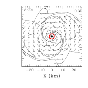
Figure 3: Snapshots of the density contour curves for $\rho$ in the equatorial plane for model SLy1414a. The solid contour curves are drawn for $\rho=2\times 10^{14}\times i~{}{\rm g/cm^{3}}~{}(i=2\sim 10)$ and for $2\times 10^{14}\times 10^{-0.5i}~{}{\rm g/cm^{3}}~{}(i=1\sim 7)$. The dotted curves denote $2\times 10^{14}~{}{\rm g/cm^{3}}$. The number in the upper left-hand side denotes the elapsed time from the beginning of the simulation in units of ms. The initial orbital period in this case is 2.012 ms. Vectors indicate the local velocity field $(v^{x},v^{y})$, and the scale is shown in the upper right-hand corner. The thick circle in the last panel of radius $r\sim 2$ km denotes the location of the apparent horizon.

Figure 4: The same as Fig. 3 but for model SLy1313a. The initial orbital period is 2.110 ms in this case.

Figure 5: The same as Fig. 3 but for model SLy125135a. The initial orbital period is 2.110 ms in this case.

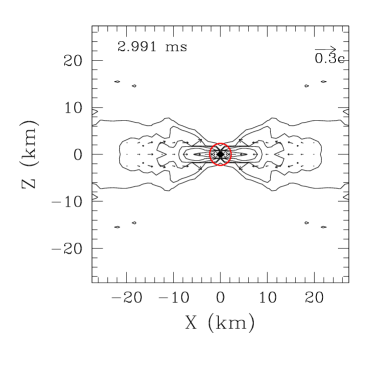
(a)   (b)

Figure 6: Snapshots of the density contour curves for $\rho$ and the local velocity field $(v^{x},v^{z})$ in the $y=0$ plane (a) at $t=2.991$ ms for model SLy1414a and (b) at $t=8.621$ ms for model SLy1313a. The method for drawing the contour curves and the velocity vectors is the same as that in Fig. 3.

Several quantities that characterize irrotational binary neutron stars in quasiequilibrium circular orbits used as initial conditions for the present simulations are summarized in Table II. We choose binaries of an orbital separation which is slightly larger than that for an innermost orbit. Here, the innermost orbit is defined as a close orbit for which Lagrange points appear at the inner edge of neutron stars USE ; GBM . If the orbital separation becomes smaller than that of the innermost orbit, mass transfer sets in and dumbbell-like structure will be formed. Until the innermost orbit is reached, the circular orbit is stable, and hence, the innermost stable circular orbit does not exist outside the innermost orbit for the present cases. However, we should note that the innermost stable circular orbit seems to be very close to the innermost orbit since the decrease rates of the energy and the angular momentum as functions of the orbital separation are very small near the innermost orbit.

The ADM mass of each neutron star, when it is in isolation (i.e., when the orbital separation is infinity), is chosen in the range between $1.2M_{\odot}$ and $1.45M_{\odot}$. Models SLy1212, SLy1313, SLy135135, SLy1414, FPS1212, FPS125125, FPS1313, and FPS1414 are equal-mass binaries, and SLy125135 and SLy135145 are unequal-mass ones. For the unequal-mass case, the mass ratio $Q_{M}$ is chosen to be $\mathrel{\raise 1.29167pt\hbox{$>$}\mkern-14.0mu\lower 2.58334pt\hbox{$\sim$}}0.9$ since all the observed binary neutron stars for which each mass is determined accurately indeed have such mass ratio Stairs . Mass of each neutron star in model SLy125135 is approximately the same as that of PSRJ0737-3039 NEW , while the mass in model SLy135145 is similar to that of PSRB1913+16 HT . The total baryon rest-mass for models SLy1313 and SLy125135 and for models SLy1414 and SLy135145 are approximately identical, respectively. For all these binaries, the orbital period of the initial condition is about 2 ms. This implies that the frequency of emitted gravitational waves is about 1 kHz.

The simulations were performed using a fixed uniform grid and assuming reflection symmetry with respect to the equatorial plane (here, the equatorial plane is chosen to be the orbital plane). The detailed simulations were performed with the SLy equation of state. In this equation of state, the used grid size is (633, 633, 317) or (377, 377, 189) for $(x,y,z)$. In the FPS equation of state, simulations were performed with the (377, 377, 189) grid size to save the computational time. The grid covers the region $-L\leq x\leq L$, $-L\leq y\leq L$, and $0\leq z\leq L$ where $L$ is a constant. The grid spacing is determined from the condition that the major diameter of each star is covered with about 50 grid points initially. We have shown that with this grid spacing, a convergent numerical result is obtained STU . The circumferential radius of spherical neutron stars with the SLy and FPS equations of state is about 11.6 and 10.7 km for $M=1.4M_{\odot}$, respectively (see Fig. 2). Thus, the grid spacing is $\sim 0.4$ km.

Accuracy in the computation of gravitational waveforms and the radiation reaction depends on the location of the outer boundaries if the wavelength, $\lambda$, is larger than $L$ STU . For $L\mathrel{\raise 1.29167pt\hbox{$<$}\mkern-14.0mu\lower 2.58334pt\hbox{$\sim$}}0.4\lambda$, the amplitude and the radiation reaction of gravitational waves are significantly overestimated STU ; SU01 . Due to the restriction of the computational power, it is difficult to take a huge grid size in which $L$ is much larger than $\lambda$. As a consequence of the present restricted computational resources, $L$ has to be chosen as $\sim 0.4\lambda_{0}$ where $\lambda_{0}$ denotes $\lambda$ of the $l=m=2$ mode at $t=0$. Hence, the error associated with the small value of $L$ is inevitable, and thus, the amplitude and radiation reaction of gravitational waves are overestimated in the early phase of the simulation. However, the typical wavelength of gravitational waves becomes shorter and shorter in the late inspiral phase, and hence, the accuracy of the wave extraction is improved with the evolution of the system. This point will be confirmed in Sec. III.

The wavelength of quasiperiodic gravitational waves emitted from the formed hypermassive neutron star (denoted by $\lambda_{\rm merger}$) is much shorter than $\lambda_{0}$ and as large as $L$ (see Table III), so that the waveforms in the merger stage are computed accurately (within $\sim 10\%$ error) in the case of neutron star formation irrespective of the grid size. We performed simulations for models SLy1313, SLy125135, SLy1414, and SLy135145 with the two grid sizes, and confirmed that this is indeed the case. We demonstrate this fact in Sec. III by comparing the results for models SLy1313a and SLy1313b. From the numerical results for four models, we have also confirmed that the outcome in the merger does not depend on the grid size. Thus, when we are interested in the outcome or in gravitational waves emitted by the hypermassive neutron stars, simulations may be performed in a small grid size such as (377, 377, 189).

With the (633, 633, 317) grid size, about 240 GBytes computational memory is required. For the case of the hypermassive neutron star formation, the simulations are performed for about 30,000 time steps (until $t\sim 10$ ms) and then stopped to save the computational time. The computational time for one model in such a simulation is about 180 CPU hours using 32 processors on FACOM VPP5000 in the data processing center of National Astronomical Observatory of Japan (NAOJ). For the case of the black hole formation, the simulations crash soon after the formation of apparent horizon because of the so-called grid stretching around the black hole formation region. In this case, the computational time is about 60 CPU hours for about 10,000 time steps.

III.2 Characteristics of the merger

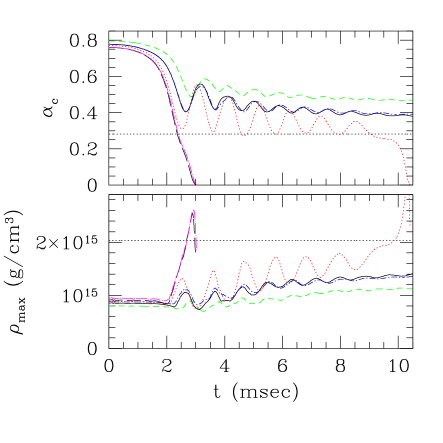
(a)     (b)

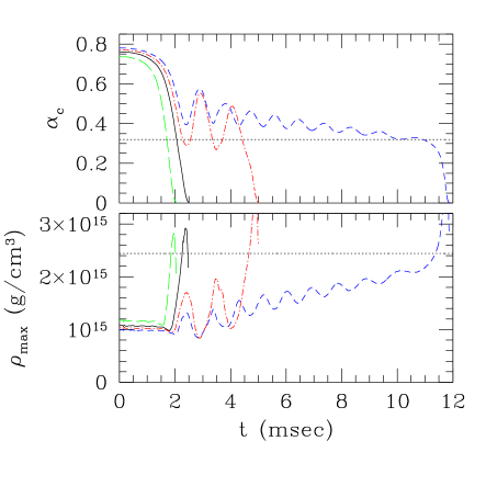
Figure 7: Evolution of the maximum values of $\rho$ and the central value of $\alpha$ (a) for models SLy1414a (long dashed curves), SLy135145a (dotted long-dashed curves which approximately coincide with long dashed curve for $\alpha_{c}$), SLy135135b (dotted curves), SLy1313a (solid curves), SLy125135a (dotted dashed curves), and SLy1212b (dashed curves), and (b) for models FPS1414b (long dashed curves), FPS1313b (solid curves), FPS125125 (dotted-dashed curves), and FPS1212b (dashed curves). The dotted horizontal lines denote the central values of the lapse and density of the marginally stable and spherical star in equilibrium for given cold equations of state. The reason that the maximum density decreases in the final stage for the black hole formation case is as follows: We choose $\rho_{*}$ as a fundamental variable to be evolved and compute $\rho$ from $\rho_{*}/(\alpha u^{t}e^{6\phi})$. In the final stage, $\phi$ is very large ($>1$) and, hence, a small error in $\phi$ results in a large error in $\rho$. Note that the maximum value of $\rho_{*}$ increases monotonically by many orders of magnitude.

(a)    (b)

Figure 8: Evolution of the angular velocity $\Omega$ along $x$ (solid curves) and $y$ (dashed curves) axes (a) for models SLy1313a and (b) SLy125135a. The time is shown in the upper right corner of each panel in units of ms. $\Omega$ along $x$ and $y$ axes is computed by $v^{y}/x$ and $v^{x}/y$, and hence, it is not determined at the origin. Since the formed hypermassive neutron star is not spheroidal, $\Omega$ along two axes is significantly different.

III.2.1 General feature

In Figs. 3–5, we display the snapshots of the density contour curves and the velocity vectors in the equatorial plane at selected time steps for models SLy1414a, SLy1313a, and SLy125135a, respectively. Figure 6 displays the density contour curves and the velocity vectors in the $y=0$ plane at a late time for SLy1414a and SLy1313a. Figures 3 and 6(a) indicate typical evolution of the density contour curves in the case of prompt black hole formation. On the other hand, Figs. 4, 5, and 6(b) show those in the formation of hypermassive neutron stars.

Figure 7 displays the evolution of the maximum value of $\rho$ (hereafter $\rho_{\rm max}$) and the central value of $\alpha$ (hereafter $\alpha_{c}$) for models SLy1414a, SLy135145a, SLy135135b, SLy1313a, SLy125135a, and SLy1212b (Fig. 7(a)) and for models FPS1414b, FPS1313b, FPS125125b, and FPS1212b (Fig. 7(b)). This shows that in the prompt black hole formation, $\alpha_{c}$ monotonically decreases toward zero. On the other hand, $\alpha_{c}$ and $\rho_{\rm max}$ settle down to certain values in the hypermassive neutron star formation. For model SLy135135b, a hypermassive neutron star is formed first, but after several quasiradial oscillations of high amplitude, it collapses to a black hole due to dissipation of the angular momentum by gravitational radiation. The large oscillation amplitude results from the fact that the selfgravity is large enough to deeply shrink surmounting the centrifugal force. These indicate that the total ADM mass of this model ($M\approx 2.7M_{\odot}$) is only slightly smaller than the threshold value for the prompt black hole formation. The quasiradial oscillation of the large amplitude induces a characteristic feature in gravitational waveforms and the Fourier spectrum (cf. Sec. III.3).

In the case of black hole formation (models SLy1414, SLy135145, SLy135135, FPS1414, FPS1313, FPS125125, and FPS1212), the computation crashed soon after the formation of apparent horizons since the region around the apparent horizon of the formed black hole was stretched significantly and the grid resolution became too poor to resolve such region. On the other hand, we stopped the simulations for other cases to save the computational time, after the evolution of the formed massive neutron stars was followed for a sufficiently long time. At the termination of these simulations, the averaged violation of the Hamiltonian constraint $H$ remains of order 0.01 (cf. Fig. 18). We expect that the simulations could be continued for a much longer time than $10$ ms if we could have sufficient computational time.

In every model, the binary orbit is stable at $t=0$ and the orbital separation gradually decreases due to the radiation reaction of gravitational waves for which the emission time scale is longer than the orbital period. If the orbital separation becomes sufficiently small, each star is elongated by tidal effects. As a result, the attraction force due to the tidal interaction between two stars becomes strong enough to make the orbit unstable to merger. The merger starts after about one orbit at $t\sim 2$ ms irrespective of models. Since the orbital separation at $t=0$ is very close to that for a marginally stable orbit, a small decrease of the angular momentum and energy is sufficient to induce the merger in the present simulations. If the total mass of the system is high enough, a black hole is directly formed within about 1 ms after the merger sets in. On the other hand, for models with mass smaller than a threshold mass $M_{\rm thr}$, a hypermassive neutron star is formed at least temporarily. The hypermassive neutron star is stable against gravitational collapse for a while after its formation, but it will collapse to a black hole eventually due to radiation reaction of gravitational waves or due to outward angular momentum transfer (see discussion later).

In the formation of the hypermassive neutron stars, a double core structure is first formed, and then, it relaxes to a highly nonaxisymmetric ellipsoid (cf. Figs. 4, 5, and 6(b)). The contour plots drawn for a high-density region with $\rho\geq 4\times 10^{14}~{}{\rm g/cm^{3}}$ show that the axial ratio of the bar measured in the equatorial plane is $\sim 0.5$; the axial lengths of the semi major and minor axes are $\sim 20$ and 10 km, respectively. Figure 6(b) also shows that the axial length along the $z$ axis is about 10 km. Namely, a highly elliptical rotating ellipsoid is formed. This outcome is significantly different from the previous ones found with the $\Gamma=2$ equation of state STU , in which nearly axisymmetric spheroidal neutron stars are formed. The reason is that the adiabatic index of the realistic equations of state adopted in this paper is much larger than 2 that is adopted in the previous one. According to a Newtonian study james , a uniformly rotating ellipsoid (Jacobi-like ellipsoid) exists only for $\Gamma\mathrel{\raise 1.29167pt\hbox{$>$}\mkern-14.0mu\lower 2.58334pt\hbox{$\sim$}}2.25$. This fact suggests that rapidly rotating stars with a large adiabatic index are only subject to the ellipsoidal deformation. Note that similar results have been already reported in Newtonian and post Newtonian simulations RS ; C ; FR .

The rotating hypermassive neutron stars also oscillate in a quasiradial manner (cf. Fig. 7). Such oscillation is induced by the approaching velocity at the collision of two stars. By the radial motion, shocks are formed at the outer region of the hypermassive neutron stars to convert the kinetic energy to the thermal energy. The shocks are also generated when the spiral arms hit the oscillating hypermassive neutron stars. These shocks heat up the outer region of the hypermassive neutron stars for many times, and as a result, the thermal energy of the envelope increases fairly uniformly. The further detail of these thermal properties is discussed in Sec. III.2.3.

Since the degree of the nonaxial symmetry is sufficiently large, the hypermassive neutron star found in this paper is a stronger emitter of gravitational waves than that found in STU . The significant radiation decreases the angular momentum of the hypermassive neutron stars. The nonaxisymmetric structure also induces the angular momentum transfer from the inner region to the outer one due to the hydrodynamic interaction. As a result of these effects, the rotational angular velocity $\Omega=v^{\varphi}$ decreases and its profile is modified. In Fig. 8, we show the evolution of $\Omega$ of the hypermassive neutron stars along $x$ and $y$ axes at $t=3.897$, 6.069, and 8.621 ms for models SLy1313a and SLy125135a. At its formation, the hypermassive neutron stars are strongly differentially and rapidly rotating. The strong differential rotation yields the strong centrifugal force, which plays an important role for sustaining the large selfgravity of the hypermassive neutron stars BSS ; SBS . Since the angular momentum is dissipated by the gravitational radiation and redistributed by the hydrodynamic interaction, $\Omega$ decreases significantly in the central region, and hence, the steepness of the differential rotation near the center decreases with time. This effect eventually induces the collapse to a black hole.

It should be also noted that $\Omega$ along two axes is significantly different near the origin. The reason at $t=3.897$ ms is that the formed hypermassive neutron stars have a double-core structure (cf. Figs. 4 and 5) and the angular velocity of the cores are larger than the low density region surrounding them. The reason for $t\mathrel{\raise 1.29167pt\hbox{$>$}\mkern-14.0mu\lower 2.58334pt\hbox{$\sim$}}6$ ms is that the hypermassive neutron star is not a spheroid but an ellipsoid of high ellipticity and the angular velocity depends strongly on the coordinate $\varphi$.

Figures 4 and 5 show that even after the emission of gravitational waves for $\sim$ 10 ms, the hypermassive neutron star is still highly nonaxisymmetric. This indicates that gravitational waves will be emitted for much longer time scale than 10 ms. Thus, the rotational kinetic energy and the angular momentum will be subsequently dissipated by a large factor, eventually inducing the collapse to a black hole.

We here estimate the lifetime of the hypermassive neutron stars using Fig. 7 which shows that the value of $\alpha_{c}$ decreases gradually with time. It is reasonable to expect that the collapse to a black hole sets in when the value of $\alpha_{c}$ becomes smaller than a critical value. Since the angular momentum should be sufficiently dissipated before the collapse sets in, the threshold value of $\alpha_{c}$ for the onset of the collapse will be approximately equal to that of marginally stable spherical stars (i.e., the dotted horizontal line in Fig. 7). One should keep in mind that the threshold value depends on the slicing condition, and thus, this method can work only when the same slicing is used for computation of the spherical star and for simulation. In this paper, the (approximate) maximal slicing is adopted both in the simulation and in computation of spherical equilibria so that this method can be used. The results for models SLy135135b and FPS1212b indeed illustrate that the prediction by this method is appropriate.

For models SLy1313a, SLy125135a and SLy1212b, the decrease rate of the value of $\alpha_{c}$ estimated from the data for 5 ms $\mathrel{\raise 1.29167pt\hbox{$<$}\mkern-14.0mu\lower 2.58334pt\hbox{$\sim$}}t\mathrel{\raise 1.29167pt\hbox{$<$}\mkern-14.0mu\lower 2.58334pt\hbox{$\sim$}}10$ ms is $\sim 0.005$ ${\rm ms}^{-1}$. Extrapolating this result suggests that the hypermassive neutron stars will collapse to a black hole at $t\sim 30$ ms for models SLy1313a and SLy125135a and at $t\sim 50$ ms for model SLy1212b. These time scales are much shorter than the dissipation time scale by viscosities or the redistribution time scale of the angular momentum by the magnetic field BSS . Therefore, the gravitational radiation or the outward angular momentum transfer by the hydrodynamic interaction plays the most important role in the evolution of the hypermassive neutron stars.

In the prompt formation of a black hole, most of the fluid elements are swallowed into the black hole in 1 ms after the merger sets in. Thus, the final outcome is a system of a rotating black hole and a surrounding disk of very small mass (cf. Fig. 6(a)). In Fig. 9, we plot the evolution of the total baryon rest-mass located outside a radius $r$, $M_{*}(r)$, for models SLy1414a and SLy135145a. $M_{*}(r)$ is defined by

$$M_{*}(r)=\int_{r\leq r^{\prime}\leq r_{\rm max}}\rho_{*}d^{3}x^{\prime},$$ (39)

where $r_{\rm max}$ is introduced to exclude the contribution from the small-density atmosphere. In the present work we choose as $r_{\rm max}=7.5M_{0}\approx 31$ km within which the integrated mass of the atmosphere is negligible ($<$0.01% of the total mass). The results are plotted for $r/M_{0}=1.5$, 3, and 4.5. Note that the apparent horizon is located for $r\approx 0.5M_{0}$ at $t\approx 3.0$ ms for models SLy1414a and SLy135145a, and inside the horizon about 99% and 98% of the initial mass are enclosed for these cases, respectively. Figure 9 indicates that the fluid elements still continue to fall into the black hole at the end of the simulation. This suggests that the final disk mass will be smaller than 1% of the total baryon rest-mass.

In STU , we found that even the small mass difference with $Q_{M}\sim 0.9$ increases the fraction of disk mass around the black hole significantly. However, in the present equations of state, $Q_{M}\sim 0.9$ is not small enough to significantly increase the disk mass. This results from the difference in the equations of state. The detailed reason is discussed in Sec. III.2.4.

The area of the apparent horizons $A$ is determined in the black hole formation cases. We find that

$${A\over 16\pi M_{0}^{2}}\sim 0.85,$$ (40)

for models SLy1414a and SLy135145a. Since most of the fluid elements are swallowed into the black hole and also the energy carried out by gravitational radiation is at most $\sim 0.01M_{0}$ (cf. Fig. 18), the mass of the formed black hole is approximately $\sim 0.99M_{0}$. Assuming that the area of the apparent horizon is equal to that of the event horizon, the nondimensional spin parameter of the black hole defined by $q\equiv J_{\rm BH}/M_{\rm BH}^{2}$, where $J_{\rm BH}$ and $M_{\rm BH}$ are the angular momentum and the mass of the black hole, are computed from

$${A\over 16\pi M_{\rm BH}^{2}}={1\over 2}\Bigl{[}1+(1-q^{2})^{1/2}\Bigr{]}.$$ (41)

Equation (41) implies that for $A/16\pi M_{\rm BH}^{2}\sim 0.85$, $q\sim 0.7$.

On the other hand, we can estimate the value of $q$ in the following manner. As shown in Sec. III.3, the angular momentum is dissipated by $\sim 10$–15% by gravitational radiation, while the ADM mass decreases by $\sim 1\%$. As listed in Table II, the initial value of $q$ is $\sim 0.9$. Therefore, the value of $q$ in the final stage should be $\sim 0.75$–0.8. The values of $q$ derived by two independent methods agree with each other within $\sim 10\%$ error. This indicates that the location and the area of the black holes are determined within $\sim 10\%$ error.

For $q=0.7$–0.8 and $M_{\rm BH}\approx 2.8M_{\odot}$, the frequency of the quasinormal mode for the black hole oscillation is about 6.5–7$(2.8M_{\odot}/M_{\rm BH})$ kHz Leaver . This value is rather high and far out of the best sensitive frequency range of the laser interferometric gravitational wave detectors KIP . Thus, in the following, we do not touch on gravitational waveforms in the prompt black hole formation.

III.2.2 Threshold mass for black hole formation

The threshold value of the total ADM mass above which a black hole is promptly formed is $M_{\rm thr}\sim 2.7M_{\odot}$ for the SLy equation of state and $M_{\rm thr}\sim 2.5M_{\odot}$ for the FPS one with $\Gamma_{\rm th}=2$. For the SLy case, we find that the value does not depend on the mass ratio for $0.9\mathrel{\raise 1.29167pt\hbox{$<$}\mkern-14.0mu\lower 2.58334pt\hbox{$\sim$}}Q_{M}\leq 1$. The maximum allowed mass for the stable and spherical neutron stars is $2.04M_{\odot}$ and $1.80M_{\odot}$ for the SLy and FPS equations of state, respectively. This implies that if the total mass is by $\sim 30$–40% larger than the maximum allowed mass for stable and spherical stars, a black hole is promptly formed. In a previous study with the $\Gamma=2$ equation of state STU , we found that threshold mass is by about 70% larger than the maximum allowed mass for stable and spherical neutron stars. Thus, comparing the threshold value of the total ADM mass, we can say that a black hole is more subject to be formed promptly with the realistic equations of state.

In LBS ; MBS , the maximum mass of differentially rotating stars in axisymmetric equilibrium (hereafter $M_{\rm max:dif}$) is studied for various equations of state. The authors compare $M_{\rm max:dif}$ with the maximum mass of spherical stars (hereafter $M_{\rm max:sph}$) for given equations of state. They find that the ratio $M_{\rm max:dif}/M_{\rm max:sph}$ for FPS and APR equations of state (APR is similar to SLy equation of state) is much smaller than that for $\Gamma=2$ equation of state. Their study is carried out for axisymmetric rotating stars in equilibrium and with a particular rotational law, and hence, their results cannot be simply compared with our results obtained for dynamical and nonaxisymmetric spacetime. However, their results suggest that the merged object may be more susceptible to collapse to a black hole with the realistic equations of state. This tendency agrees with our conclusion.

The compactness in each neutron star of no rotation in isolation is defined by $C=GM_{\rm sph}/R_{\rm sph}c^{2}$ where $M_{\rm sph}$ and $R_{\rm sph}$ denote the ADM mass and the circumferential radius of the spherical stars. For the SLy equation of state, $C\approx 0.151$, 0.165, 0.172, and 0.178 for $M_{\rm sph}=1.2$, 1.3, 1.35, and $1.4M_{\odot}$, respectively. For FPS one, $C\approx 0.162$, 0.169, 0.177, and 0.192 for $M_{\rm sph}=1.2$, 1.25, 1.3, and $1.4M_{\odot}$, respectively. This indicates that a black hole is promptly formed for $C\mathrel{\raise 1.29167pt\hbox{$>$}\mkern-14.0mu\lower 2.58334pt\hbox{$\sim$}}0.17$ after merger of two (nearly) identical neutron stars. In the $\Gamma=2$ equation of state, the threshold value of $C$ is $\sim 0.15$–0.16 STU . Thus, comparing the threshold value of the compactness, we can say that a black hole is less subject to be formed with the realistic equations of state.

The reason that the threshold mass for the prompt black hole formation is smaller with the realistic equations of state may be mentioned in the following manner: In the realistic equations of state, the compactness of each neutron star is larger than that with the $\Gamma=2$ equation of state for a given mass. Accordingly, for a given total mass, the binary system at the onset of the merger is more compact. This implies that the angular momentum is dissipated more before the merger sets in with the realistic equations of state. In the case of the hypermassive neutron star formation, the centrifugal force plays the most important role for sustaining the large selfgravity. Thus, the large dissipation of the angular momentum before the merger helps the prompt black hole formation. Therefore, a black hole is more subject to be formed in the realistic equations of state.

III.2.3 Thermal properties

.

In Fig. 10(a)–(c), we show profiles of $\varepsilon$ and $\varepsilon_{\rm th}$ as well as that of $\rho$ along $x$ and $y$ axes at $t=2.991$ ms for model SLy1414a, at $t=8.621$ ms for model SLy1313a, and at $t=8.621$ ms for model SLy125135a, respectively. The density contour curves at the corresponding time steps are displayed in the last panel of Figs. 3–5. Figure 10(d) shows the evolution of the total internal energy and thermal energy defined by

$$U\equiv\int\rho_{*}\varepsilon d^{3}x,$$ (42)

$$U_{\rm th}\equiv\int\rho_{*}\varepsilon_{\rm th}d^{3}x,$$ (43)

for models SLy1313a, SLy125135a, and SLy1212b. Note that in the absence of shock heating, $\varepsilon$ should be equal to $\varepsilon_{\rm cold}$. Thus, $\varepsilon_{\rm th}$ denotes the specific thermal energy generated by the shock heating.

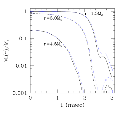
Figure 9: Evolution of $M_{*}(r)/M_{*}$ for $r=1.5$, 3, and $4.5M_{0}$ for models SLy1414a (curves except for the dotted curve) and SLy135145a (dotted curves). $M_{0}$ and $M_{*}$ denote the ADM mass and total baryon rest-mass of binary neutron stars at $t=0$. Definition for $M_{*}(r)$ is shown in Eq. (39).

(a)    (b)

(c)    (d)

Figure 10: Profiles of $\varepsilon$ (solid curves) and $\varepsilon_{\rm th}=\varepsilon-\varepsilon_{\rm cold}$ (dashed curves) as well as that of $\rho$ along $x$ and $y$ axes (a) at $t=2.991$ ms for model SLy1414a, (b) at $t=8.621$ ms for model SLy1313a, and (c) at $t=8.621$ ms for model SLy125135a. Note that the region of $r\mathrel{\raise 1.29167pt\hbox{$<$}\mkern-14.0mu\lower 2.58334pt\hbox{$\sim$}}2$ km for panel (a) is inside the apparent horizon (see Figs. 3 and 6(a)). (d) Evolution of $U$ and $U_{\rm th}$ in unit of the rest-mass energy $M_{*}c^{2}$ for models SLy1313a (solid curves), SLy125135a (dotted curves), and SLy1212b (dashed curves).

First, we focus on the thermal property for models SLy1313a and SLy125135a which are the representative models of hypermassive neutron star formation. In these cases, the heating is not very important in the central region. This is reasonable because the shocks generated at the collision of two stars are not very strong, and thus, the central part of the hypermassive neutron stars is formed without experiencing the strong shock heating. On the other hand, the shock heating plays an important role in the outer region of the hypermassive neutron stars and in the surrounding accretion disk since the spiral arms hit the hypermassive neutron stars for many times.

The typical value of $\varepsilon_{\rm th}$ is $0.01c^{2}$–$0.02c^{2}$. Here, we recover $c$ for making the unit clear. In the following, we assume that the components of the hypermassive neutron stars and surrounding disks are neutrons. Then, the value of $\varepsilon_{\rm th}=0.01c^{2}$ implies that the thermal energy per nucleon is

$$9.37\biggl{(}{\varepsilon_{\rm th}\over 0.01c^{2}}\biggr{)}~{}{\rm MeV/nucleon}.$$ (44)

Since the typical value of $\varepsilon_{\rm th}$ is $0.01c^{2}$–$0.02c^{2}$, the typical thermal energy is 10–20 MeV. This value agrees approximately with that computed in RJ ; RJ2 .

Figure 10(d) shows that the total internal energy and thermal energy are relaxed to be

$$U\sim 0.1M_{*}c^{2}\sim 5\times 10^{53}~{}{\rm erg},$$ (45)

$$U_{\rm th}\sim 0.025M_{*}c^{2}\sim 1\times 10^{53}~{}{\rm erg},$$ (46)

for both models SLy1313a and SLy125135a. Thus, the thermal energy increases up to $\sim 25\%$ of the total internal energy. We note that these values are approximately identical between models SLy1313a and SLy125135a. This implies that the mass ratio of $Q_{M}\sim 0.9$ does not significantly modify the thermal properties of the hypermassive neutron stars in the realistic equations of state.

The region of $\varepsilon_{\rm th}\sim 0.01c^{2}$ will be cooled via the emission of neutrinos RJ ; RJ2 . According to RJ ; RJ2 , the emission rate in the hypermassive neutron star with the averaged value of $\varepsilon_{\rm th}\sim 10$–30 MeV is $10^{52}$–$10^{53}$ erg/s. Thus, if all the amounts of the thermal energy are assumed to be dissipated by the neutrino cooling, the time scale for the emission of the neutrinos will be 1–10 s. This is much longer than the lifetime of the hypermassive neutron stars $\mathrel{\raise 1.29167pt\hbox{$<$}\mkern-14.0mu\lower 2.58334pt\hbox{$\sim$}}100$ ms. Therefore, the cooling does not play an important role in their evolution.

Since the lifetime of the hypermassive neutron stars $\mathrel{\raise 1.29167pt\hbox{$<$}\mkern-14.0mu\lower 2.58334pt\hbox{$\sim$}}100$ ms is nearly equal to the time duration of the short gamma-ray bursts GRB , it is interesting to ask if they could generate the typical energy of the bursts. In a model for central engines of the gamma-ray bursts, a fireball of the electron-positron pair and photon is produced by the pair annihilation of the neutrino and antineutrino RJ2 ; GRB . In RJ2 , Janka and Ruffert estimate the efficiency of the annihilation as several$\times 10^{-3}$ for the neutrino luminosity $\sim 10^{52}$ erg/s, the mean energy of neutrino $\sim 10$ MeV, and the radius of the hypermassive neutron star $\sim 10$ km (see Eq. (1) of RJ2 ). This suggests that the energy generation rate of the electron-positron pair is $\sim 10^{50}$ erg/s. Since the lifetime of the hypermassive neutron stars is $\mathrel{\raise 1.29167pt\hbox{$<$}\mkern-14.0mu\lower 2.58334pt\hbox{$\sim$}}100$ ms, the energy available for the fireball will be at most $\sim 10^{49}$ erg. This value is not large enough to explain typical cosmological gamma-ray bursts. Furthermore, as Janka and Ruffert found RJ2 , the pair annihilation of the neutrino and antineutrino is most efficient in a region near the hypermassive neutron star, for which the baryon density is large enough (cf. Fig. 6(b)) to convert the energy of the fireball to the kinetic energy of the baryon. Therefore, it is not very likely that the hypermassive neutron stars are the central engines of the typical short gamma-ray bursts.

Now, we focus on model SLy1414a in which a black hole is promptly formed after the merger. Comparing Fig. 10(a) with the last panel of Fig. 3, the region of high thermal energy is located along the spiral arms of the accretion disk surrounding the central black hole. (Note that the region of $r\mathrel{\raise 1.29167pt\hbox{$<$}\mkern-14.0mu\lower 2.58334pt\hbox{$\sim$}}2$ km is inside the apparent horizon, and hence, we do not consider such region.) The part of the matter in the spiral arms with small orbital radius $r\mathrel{\raise 1.29167pt\hbox{$<$}\mkern-14.0mu\lower 2.58334pt\hbox{$\sim$}}5$ km is likely to be inside the radius of an innermost stable circular orbit around the black hole, and hence, be swallowed into the black hole. Otherwise, the matter in the spiral arms will form an accretion disk surrounding the black hole. Thus, eventually a hot accretion disk will be formed. However, the region of high thermal energy for $r\mathrel{\raise 1.29167pt\hbox{$>$}\mkern-14.0mu\lower 2.58334pt\hbox{$\sim$}}10$ km is of low density with $\rho\mathrel{\raise 1.29167pt\hbox{$<$}\mkern-14.0mu\lower 2.58334pt\hbox{$\sim$}}10^{12}~{}{\rm g/cm^{3}}$, and the total mass of the disk will be $10^{-3}M_{\odot}\mathrel{\raise 1.29167pt\hbox{$<$}\mkern-14.0mu\lower 2.58334pt\hbox{$\sim$}}M_{*}\mathrel{\raise 1.29167pt\hbox{$<$}\mkern-14.0mu\lower 2.58334pt\hbox{$\sim$}}0.01M_{\odot}$ (see Fig. 9). The total thermal energy of the accretion disk is estimated as

$$U_{\rm th} \sim M_{\rm disk}\bar{\varepsilon}_{\rm th}$$ (47)

$$=1.8\times 10^{50}\biggl{(}{M_{\rm disk}\over 0.01M_{\odot}}\biggr{)}\biggl{(}{\bar{\varepsilon}_{\rm th}\over 0.01c^{2}}\biggr{)}~{}{\rm erg}.$$

where $M_{\rm disk}$ and $\bar{\varepsilon}_{\rm th}$ denote the mass of the accretion disk and the averaged value of the specific thermal energy. Hence, even if all the amounts of the thermal energy are dissipated by the emission of neutrinos, the total energy of the radiated neutrinos will be at most several $\times 10^{50}$ erg. According to RJ2 , the efficiency of the annihilation of the neutrino and antineutrino is several $\times 10^{-5}$ for the neutrino luminosity $\sim 10^{50}$ erg/s, the mean energy of neutrino $\sim 10$ MeV, and the disk radius $\sim 10$ km. This indicates that the energy of the fireball is at most $\sim 10^{46}$ erg. Although the density of the baryon at the region that the pair annihilation is likely to happen is small enough to avoid the baryon loading problem, this energy is too small to explain cosmological gamma-ray bursts.

III.2.4 Effects of mass difference

Comparing the evolution of the contour curves, the maximum density, and the central value of the lapse function for models SLy1313a and SLy125135a (see Figs. 4, 5, and 7(a)), it is found that the mass difference plays a minor role in the formation of a hypermassive neutron star as far as $Q_{M}$ is in the range between 0.9 and 1. Figures 7(a) and 9 also illustrate that the evolution of the system to a black hole is very similar for models SLy1414a and SLy135145a. In STU in which simulations were performed using the $\Gamma=2$ equation of state, we found that the mass difference with $Q_{M}\sim 0.9$ significantly induces an asymmetry in the merger which contributes to formation of large spiral arms and the outward angular momentum transfer, which are not very outstanding in the present results. The reason seems to be as follows. In the previous equation of state, the mass difference with $Q_{M}\sim 0.9$ results in a relatively large ($\sim 15\%$) difference of the compactness between two stars. On the other hand, the difference in the compactness between two stars with the present equations of state is $\sim 10\%$ for $Q_{M}\sim 0.9$. This is due to the fact that the stellar radius depends weakly on the mass in the range $0.8M_{\odot}\mathrel{\raise 1.29167pt\hbox{$<$}\mkern-14.0mu\lower 2.58334pt\hbox{$\sim$}}M\mathrel{\raise 1.29167pt\hbox{$<$}\mkern-14.0mu\lower 2.58334pt\hbox{$\sim$}}1.5M_{\odot}$ (see Fig. 2). As a result of the smaller difference in the compactness, the tidal effect from the more massive star to the companion becomes smaller, and therefore, the asymmetry is suppressed. To yield a system of a black hole and a massive disk, smaller mass ratio with $Q_{M}<0.9$ will be necessary in the realistic equations of state.

Another possible reason is that neutron stars in the realistic equations of state are more compact than those in the $\Gamma=2$ equation of state. Due to this fact, at the merger, the system is more compact, and hence, even in the formation of the asymmetric spiral arms, they cannot spread outward extensively but wind around the formed neutron star quickly. Consequently, the mass of the disk around the central object is suppressed to be small and also the asymmetric density configuration does not become very outstanding.

III.2.5 Dependence of dynamics on the grid size and $\Gamma_{\rm th}$

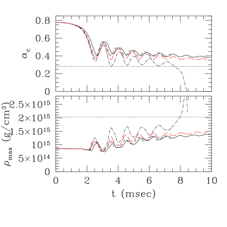
Figure 11: The same as Fig. 7 but for models SLy1313a (solid curves), SLy1313b (dashed curves), SLy1313c (dotted dashed curves), and SLy1313d (long dashed curves). Note that the simulation for SLy1313b was stopped at $t\sim 7.5$ ms to save computational time.

For model SLy1313, we performed simulations changing the value of $\Gamma_{\rm th}$ with the grid size (377, 377, 189). In Fig. 11, evolution of $\alpha_{c}$ and $\rho_{\rm max}$ is shown for models SLy1313b–SLy1313d. Note that the grid size and grid spacing are identical for these models. The results for model SLy1313a are shown together for comparison with those for model SLy1313b for which the parameters are identical but for the grid size.

By comparing the results for models SLy1313a and SLy1313b, the magnitude of the error associated with the small size of $L$ is investigated. Figure 11 shows that two results are approximately identical besides a systematic phase shift of the oscillation. This shift is caused by the inappropriate computation of the radiation reaction in the late inspiral stage for $t\mathrel{\raise 1.29167pt\hbox{$<$}\mkern-14.0mu\lower 2.58334pt\hbox{$\sim$}}2$ ms: For model SLy1313b, $L$ is smaller, and hence, the radiation reaction in the inspiral stage is significantly overestimated to spuriously accelerate the merger resulting in the phase shift. However, besides the phase shift, the results are approximately identical. In particular, the results agree well in the merging phase. This indicates that even with the smaller grid size (377, 377, 189), the formation and evolution of the hypermassive neutron star can be followed within a small error.

Comparison of the results among models SLy1313b–SLy1313d tells that for the smaller value of $\Gamma_{\rm th}$, the maximum density (central lapse) of a hypermassive neutron star formed during the merger is larger (smaller). This is due to the fact that the strength of the shock formed at the collision of two stars, which provides the thermal energy in the outer region of the formed hypermassive neutron stars to expand, is proportional to the value of $\Gamma_{\rm th}-1$. Figure 11 also indicates that the evolution of the system does not depend strongly on the value of $\Gamma_{\rm th}$ for $\Gamma_{\rm th}\mathrel{\raise 1.29167pt\hbox{$>$}\mkern-14.0mu\lower 2.58334pt\hbox{$\sim$}}1.65$. However, for $\Gamma_{\rm th}=1.3$, the formed hypermassive neutron star is very compact at its birth, and hence, collapses to a black hole in a short time scale (at $t\sim 8$ ms) after the angular momentum is dissipated by gravitational radiation. This time scale for black hole formation is much shorter than that for models SLy1313b and SLy1313d for which it would be $\sim 30$ ms. This indicates that for small values of $\Gamma_{\rm th}-1\mathrel{\raise 1.29167pt\hbox{$<$}\mkern-14.0mu\lower 2.58334pt\hbox{$\sim$}}0.3$, the collapse to a black hole is significantly enhanced.

In reality, in the presence of cooling processes such as neutrino cooling, the adiabatic index $\Gamma_{\rm th}$ decreases effectively. Such cooling mechanism may accelerate the formation of a black hole. However, the emission time scale of the neutrino is $\sim 1$–10 s as mentioned in Sec. III.2.3. Thus, the effect does not seem to be very strong.

III.3 Gravitational waveforms

III.3.1 Waveforms in the formation of hypermassive neutron stars

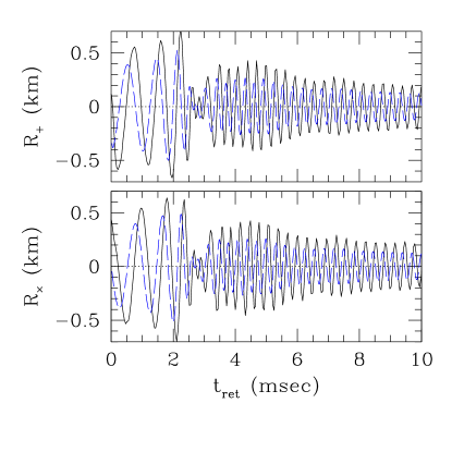
(a)    (b)

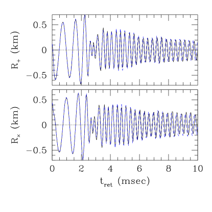
Figure 12: (a) Gravitational waves for model SLy1313a. $R_{+}$ and $R_{\times}$ (solid curves) and $A_{+}$ and $A_{\times}$ (dashed curves) as functions of the retarded time are shown. (b) $R_{+}$ and $R_{\times}$ as functions of the retarded time for model SLy125135a (solid curves). For comparison, those for SLy1313a are shown by the dashed curves.

In Figs. 12–15, we present gravitational waveforms in the formation of hypermassive neutron stars for several models. Figure 12(a) shows $R_{+}$ and $R_{\times}$ for model SLy1313a. For comparison, gravitational waves computed in terms of a quadrupole formula ($A_{+}$ and $A_{\times}$) defined in Sec. II B are shown together by the dashed curves. The amplitude of gravitational waves, $h$, observed at a distance of $r$ along the optimistic direction ($\theta=0$) is written as

$$h\approx 10^{-22}\biggl{(}{R_{+,\times}\over 0.31~{}{\rm km}}\biggr{)}\biggl{(}{100~{}{\rm Mpc}\over r}\biggr{)}.$$ (48)

Thus, the maximum amplitude observed along the most optimistic direction is $\sim 2\times 10^{-22}$ at a distance of 100 Mpc.

In the real data analysis of gravitational waves, a matched filtering technique KIP is employed. In this method, the signal of the identical frequency can be accumulated using appropriate templates, and as a result, the effective amplitude increases by a factor of $N^{1/2}$ where $N$ denotes the number of the cycle of gravitational waves for a given frequency. We determine such effective amplitude in Sec. III.3.3 (cf. Eq. (50)).

The waveforms shown in Fig. 12(a) are typical ones in the formation of a hypermassive neutron star. In the early phase ($t_{\rm ret}\mathrel{\raise 1.29167pt\hbox{$<$}\mkern-14.0mu\lower 2.58334pt\hbox{$\sim$}}2$ ms), gravitational waves associated with the inspiral motion are emitted, while for $t_{\rm ret}\mathrel{\raise 1.29167pt\hbox{$>$}\mkern-14.0mu\lower 2.58334pt\hbox{$\sim$}}2$ ms, those by the rotating and oscillating hypermassive neutron star are emitted. In the following, we focus only on the waveforms for $t_{\rm ret}\mathrel{\raise 1.29167pt\hbox{$>$}\mkern-14.0mu\lower 2.58334pt\hbox{$\sim$}}2$ ms.

Gravitational waves from the hypermassive neutron stars are characterized by quasiperiodic waves for which the amplitude and the frequency decrease slowly. The amplitude decreases with the ellipticity, which is decreased by the effects that the angular momentum decreases due to the radiation reaction and is transferred from the inner region to the outer one by the hydrodynamic interaction associated with the nonaxisymmetric structure. However, the time scale for the decrease appears to be much longer than $10$ ms as illustrated in Figs. 12–15. The oscillation frequency varies even more slowly. The reason seems to be that the following two effects approximately cancel each other: (i) with the decrease of the angular momentum of the hypermassive neutron stars due to the radiation reaction as well as the angular momentum transfer by the hydrodynamic interaction with outer envelope, the characteristic frequency of the figure rotation decreases, while (ii) with the decrease of the angular momentum, the centrifugal force is weakened to reduce the characteristic radius for a spin-up. (We note that the radiation reaction alone may increase the frequency of the figure rotation LS . In the hypermassive neutron stars formed after the merger, the angular momentum transfer due to the hydrodynamic interaction is likely to play an important role for the decrease of the frequency.)

In gravitational waveforms computed in terms of the quadrupole formula (the dashed curves in Fig. 12), the amplitude is systematically underestimated by a factor of 30–40%. This value is nearly equal to the magnitude of the compactness of the hypermassive neutron star, $GM/Rc^{2}$, where $M$ and $R$ denote the characteristic mass and radius. Since the quadrupole formula is derived ignoring the terms of order $GM/Rc^{2}$, this magnitude for the error is quite reasonable. In simulations with Newtonian, post Newtonian, and approximately relativistic frameworks, gravitational waves are computed in the quadrupole formula (e.g., C ; FR ; OUPT ). The results here indicate that the amplitudes for quasiperiodic gravitational waves from hypermassive neutron stars presented in those simulations are significantly underestimated . Although the error in the amplitude is large, the wave phase is computed accurately except for a slight systematic phase shift. From the point of view of the data analysis, the wave phase is the most important information on gravitational waves. This suggests that a quadrupole formula may be a useful tool for computing approximate gravitational waves. We note that these features have been already found for oscillating neutron stars SS1 and for nonaxisymmetric protoneutron stars formed after stellar core collapse SS3 . Here, we reconfirm that the same feature holds for the merger of binary neutron stars.

In Fig. 12(b), we display gravitational waveforms for model SLy125135a. For comparison, those for SLy1313a are shown together (dashed curves). It is found that two waveforms coincide each other very well. As mentioned in Sec. III.2.4, the mass difference with $Q_{M}\sim 0.9$ does not induce any outstanding change in the merger dynamics. This fact is also reflected in the gravitational waveforms.

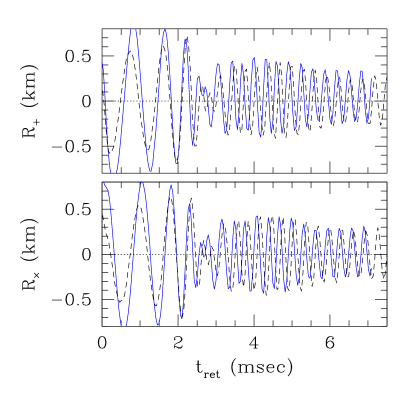
Figure 13: $R_{+}$ and $R_{\times}$ for models SLy1313a (dashed curves) and SLy1313b (solid curves) as functions of the retarded time. It is found that gravitational waveforms in the merger stage agree well. Note that the simulation for SLy1313b was stopped at $t\sim 7.5$ ms to save computational time.

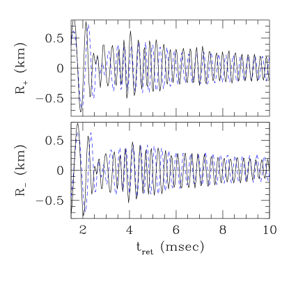
Figure 14: $R_{+}$ and $R_{\times}$ for models SLy135135b (solid curves) and SLy1313a (dashed curves) as functions of the retarded time.

In Fig. 13, we compare gravitational waveforms for models SLy1313b (solid curves) and SLy1313a (dashed curves). For SLy1313b, the simulation was performed with a smaller grid size and gravitational waves were extracted in a near zone with $L/\lambda_{0}\approx 0.25$ and $L/\lambda_{\rm merger}\approx 0.83$ (cf. for model SLy1313a, $L/\lambda_{0}\approx 0.41$ and $L/\lambda_{\rm merger}\approx 1.39$). This implies that the waveforms for model SLy1313b are less accurately computed than those for SLy1313a. Indeed, the wave amplitude for $t_{\rm ret}\mathrel{\raise 1.29167pt\hbox{$<$}\mkern-14.0mu\lower 2.58334pt\hbox{$\sim$}}2$ ms is badly overestimated. However, the waveforms from the formed hypermassive neutron stars for two models agree very well except for a systematic phase shift, which is caused by the overestimation for the radiation reaction in the early phase ($t_{\rm ret}\mathrel{\raise 1.29167pt\hbox{$<$}\mkern-14.0mu\lower 2.58334pt\hbox{$\sim$}}2$ ms). Thus, for computation of gravitational waves from the hypermassive neutron stars, we may choose the small grid size. Making use of this fact, we compare gravitational waveforms among several models computed with the small grid size in the following.

In Fig. 14, we compare gravitational waves from the hypermassive neutron stars for models SLy1313a (dashed curves) and SLy135135b (solid curves). As shown in Figs. 12 and 13, quasiperiodic waves for which the frequency is approximately constant are emitted for model SLy1313a. On the other hand, the frequency is not constant but modulates with time for model SLy135135b (e.g., see the waveforms at $t_{\rm ret}\approx 3.6$, 4.6, 5.6, and 6.6 ms for which the wavelength is relatively short). The reason is that the formed hypermassive neutron star quasiradially oscillates with a large amplitude and the frequency of gravitational waves varies with the change of the characteristic radius. Due to this, the Fourier spectra for models SLy1313 and SLy135135 are significantly different although the difference of the total mass is very small (cf. Fig. 17(b)).

In Fig. 15(a), we compare gravitational waveforms for models SLy1313b (dotted curves), SLy1313c (solid curves), and SLy1313d (dashed curves). For these models, the cold part of the equation of state is identical but the value of $\Gamma_{\rm th}$ is different. As mentioned in Sec. III.2.5, with the smaller values of $\Gamma_{\rm th}$, the shock heating is less efficient, and as a result, the formed hypermassive neutron star becomes more compact. Since the characteristic radius decreases, the amplitude of gravitational waves decreases and the frequency increases. This shows that the strength of the shock heating affects the amplitude and the characteristic frequency of gravitational waves.

In Fig. 15(b), we compare gravitational waveforms for models SLy1212b (solid curves) and FPS1212b (dashed curves). For these models, the equations of state are different, but the total ADM mass is approximately identical. Since the FPS equation of state is slightly softer than the SLy one, the compactness of each neutron star is larger by a factor of 5–10% (cf. Fig. 1) and so is for the formed hypermassive neutron star. As a result, the frequency of gravitational waves for the FPS equation of state is slightly ($\sim 15\%$) higher (cf. Fig. 17(d)). On the other hand, the amplitude of gravitational waves is not very different. This is due to the fact that with increasing the compactness, the radius of the hypermassive neutron star decreases while the angular velocity increases. These two effects approximately cancel each other, and as a result, dependence of the amplitude is not remarkable between two models.

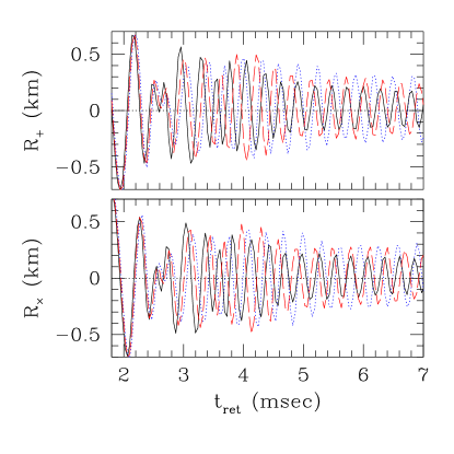
(a)    (b)

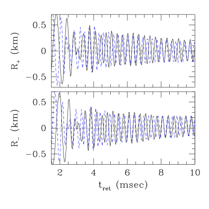
Figure 15: $R_{+}$ and $R_{\times}$ (a) for models SLy1313b (dotted curves), SLy1313c (solid curves), and SLy1313d (dashed curves), and (b) for models SLy1212b (solid curves) and FPS1212b (dashed curves) as functions of the retarded time.

III.3.2 Emission rate of the energy and the angular momentum

(a)    (b)

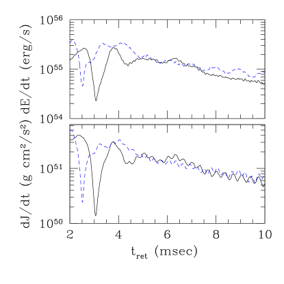
Figure 16: $dE/dt$ and $dJ/dt$ of gravitational radiation (a) for models SLy1313a (solid curves) and SLy125135a (dashed curves), and (b) for models SLy1212b (solid curves) and FPS1212b (dashed curves).

In Fig. 16(a), the emission rates of the energy and the angular momentum by gravitational radiation are shown for models SLy1313a (solid curves) and SLy125135a (dashed curves). In the inspiral phase for $t_{\rm ret}\mathrel{\raise 1.29167pt\hbox{$<$}\mkern-14.0mu\lower 2.58334pt\hbox{$\sim$}}2$ ms, they increase with time since the amplitude and the frequency of the chirp signal increase. After the peak is reached, the emission rates quickly decrease by about one order of magnitude since the merged object becomes a fairly axisymmetric transient object. However, because of its large angular momentum, the formed hypermassive neutron star soon changes to a highly ellipsoidal object which emits gravitational waves significantly. The luminosity from the ellipsoidal neutron star is as high as the first peak at $t_{\rm ret}\sim 2.2$ ms. This is in contrast with the results obtained with the $\Gamma=2$ equation of state in which the magnitude of the second peak is 30–50% as large as that of the first peak bina2 . This reflects the fact that the degree of the ellipticity of the formed hypermassive neutron star is much higher than that found in bina2 because of the large adiabatic index for the realistic equations of state.

The emission rates of the energy and the angular momentum via gravitational waves gradually decrease with time, since the degree of the nonaxial symmetry decreases. However, the decrease rates are not very large and the emission rates at $t_{\rm ret}\sim 10$ ms remain to be as high as that in the late inspiral phase as $dE/dt\sim 7\times 10^{54}$ erg/s and $dJ/dt\sim 7\times 10^{50}~{}{\rm g~{}cm^{2}/s^{2}}$. The angular momentum at $t\sim 10$ ms is $J\sim 0.7J_{0}\sim 4\times 10^{49}~{}{\rm g~{}cm^{2}/s}$. Assuming that the emission rate of the angular momentum does not change and remains $\sim 7\times 10^{50}~{}{\rm g~{}cm^{2}/s}$, the emission time scale is evaluated as $J/(dJ/dt)\sim 50$ ms. For more accurate estimation, we should compute $(J-J_{\rm min})/(dJ/dt)$ where $J_{\rm min}$ denotes the minimum allowed angular momentum for sustaining the hypermassive neutron star. Since $J_{\rm min}$ is not clear, we set $J_{\rm min}=0$. Thus, the estimated value presented here is an approximate upper limit for the emission time scale (see discussion below), and hence, the hypermassive neutron star will collapse to a black hole within 50 ms. This estimate agrees with the value $\sim 30$ ms obtained in terms of the change rate of $\alpha_{c}$ (cf. Sec. III.2.1). Therefore, we conclude that the lifetime of the hypermassive neutron stars and hence the time duration of the emission of quasiperiodic gravitational waves are as short as $\sim 30$–50 ms for models SLy1313a and SLy125135a.

Figure 16(b) displays the emission rates of the energy and the angular momentum for models SLy1212b (solid curves) and FPS1212b (dashed curves). For these models, the value of $L$ is not large enough to accurately compute gravitational waves in the inspiral phase for $t_{\rm ret}\mathrel{\raise 1.29167pt\hbox{$<$}\mkern-14.0mu\lower 2.58334pt\hbox{$\sim$}}2$ ms. Thus, we only present the results for the merger phase. The emission rates for SLy1212b are slightly smaller than those for model SLy1313a. This results from the fact that the total mass of the system is smaller. On the other hand, the emission rates for FPS1212b is slightly larger than that for SLy1212b. The reason is that the FPS equation of state is softer than the SLy one, and as a result, the formed hypermassive neutron star is more compact and the rotational angular velocity is larger. The hypermassive neutron star formed for FPS1212b collapses to a black hole at $t\sim 10$ ms. This is induced by the emission of the angular momentum by gravitational waves. However, the collapse time is shorter than the emission time scale evaluated by $J/(dJ/dt)$. This is reasonable because the hypermassive neutron star formed for model FPS1212 is close to the marginally stable configuration, and hence, a small amount of the dissipation leads to the collapse. This illustrates that the time scale $J/(dJ/dt)$ should be regarded as the approximate upper limit for the collapse time scale.

III.3.3 Fourier power spectrum

(a)    (b)

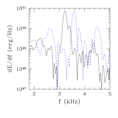
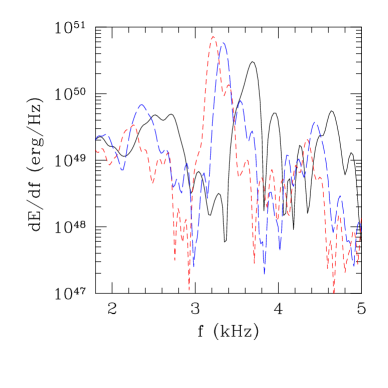
(c)    (d)

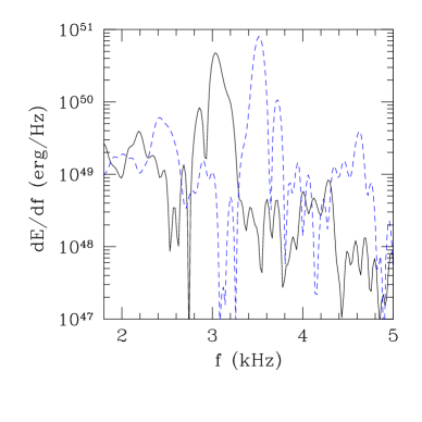
Figure 17: Fourier power spectrum of gravitational waves $dE/df$ (a) for models SLy1313a (solid curve) and SLy125135a (dashed curve), (b) for models SLy1313a (solid curve) and SLy135135b (dashed curve), (c) for models SLy1313a (dashed curve), SLy1313c (solid curve), and SLy1313d (long-dashed curve), and (d) for models SLy1212b (solid curve) and FPS1212b (dashed curve). Since the simulations are started when the frequency of gravitational waves is $\sim 1$ kHz, the spectrum for $f<1$ kHz is not correct. The dotted curve in the panel (a) denotes the analytical result of $dE/df$ in the second post Newtonian and point-particle approximation. The real spectrum for $f\mathrel{\raise 1.29167pt\hbox{$<$}\mkern-14.0mu\lower 2.58334pt\hbox{$\sim$}}1$ kHz is approximated by the dotted curves.

(a)    (b)

Figure 18: Evolution of ADM mass and angular momentum in units of their initial values $M_{0}$ and $J_{0}$, and violation of the Hamiltonian constraint (a) for model SLy1313a and (b) for model SLy1414a. In the upper two panels, the solid curves denote $M/M_{0}$ and $J/J_{0}$ computed from Eqs. (25) and (26), while the long dashed curves denote $1-\Delta E(t)/M_{0}$ and $1-\Delta J(t)/J_{0}$, respectively (see Eqs. (27) and (28)).

To determine the characteristic frequency of gravitational waves, we carried out the Fourier analysis. In Fig. 17, the power spectrum $dE/df$ is presented (a) for models SLy1313a and SLy125135a, (b) for SLy1313a and SLy135135b, (c) for SLy1313a, SLy1313c, SLy1313d, and (d) for SLy1212b and FPS1212b, respectively. Since the simulations were started with the initial condition of the orbital period $\sim 2$ ms (i.e., frequency of gravitational waves is $\sim 1$ kHz), the spectrum of inspiraling binary neutron stars for $f<1$ kHz cannot be taken into account. Thus, only the spectrum for $f\mathrel{\raise 1.29167pt\hbox{$>$}\mkern-14.0mu\lower 2.58334pt\hbox{$\sim$}}1$ kHz should be paid attention. In the panel (a), we plot the following Fourier power spectrum of two point particles in circular orbits in the second post Newtonian approximation blanchet :

$${dE\over df} ={\mu M\over 3f}x\biggl{[}1-\biggl{(}{3\over 2}+{\mu\over 6M}\biggr{)}x$$ (49)

$$~{}~{}~{}~{}~{}~{}+3\biggl{(}-{27\over 8}+{19\mu\over 8M}-{\mu^{2}\over 24M^{2}}\biggr{)}x^{2}\biggr{]}.$$

Here, $\mu$ and $M$ denote the reduced mass and the total mass of the binary, and $x\equiv(M\pi f)^{2/3}$. We note that the third post Newtonian terms does not significantly modify the spectrum since their magnitude is $\sim 0.01$ of the leading-order term. Thus, the dotted curve should be regarded as the plausible Fourier power spectrum for $f\mathrel{\raise 1.29167pt\hbox{$<$}\mkern-14.0mu\lower 2.58334pt\hbox{$\sim$}}1$ kHz.

Figure 17 shows that a sharp characteristic peak is present at $f=3$–4 kHz irrespective of models in which hypermassive neutron stars with a long lifetime ($\mathrel{\raise 1.29167pt\hbox{$>$}\mkern-14.0mu\lower 2.58334pt\hbox{$\sim$}}10$ ms) are formed (see also Table III for the list of the characteristic frequency). This is associated with quasiperiodic gravitational waves emitted by the formed hypermassive neutron stars. The amplitude of the peak is much higher than that in the $\Gamma=2$ equation of state STU . The reason is that with the realistic equations of state, the ellipticity of the formed hypermassive neutron stars is much larger, and as a result, quasiperiodic gravitational waves of a higher amplitude are emitted. Also, the elliptic structure of the hypermassive neutron stars is preserved for a long time duration. These effects amplify the peak amplitude in the Fourier power spectrum.

The energy power spectra for models SLy1313a and SLy125135a are very similar reflecting the fact that the waveforms for these two models are very similar (Fig. 17(a)). This indicates that the spectral shape depends very weakly on the mass ratio $Q_{M}$ as far as it is in the range between 0.9 and 1. On the other hand, three peaks are present at $f\approx 2.6$, 3.6, and 4.5 kHz in the energy power spectrum for model SLy135135b (Figs. 17(b)). Thus, the spectral shape is quite different from that for model SLy1313a although the total mass is only slightly different between two models. The reason is that the amplitude of the quasiradial oscillation of the hypermassive neutron star is very large and the characteristic radius varies for a wide range for model SLy135135b, inducing the modulation of the wave frequency. Indeed, the difference of the frequencies for the peaks is approximately equal to that of the quasiradial oscillation $\sim 1$ kHz. As a result, the intensity of the power spectrum is dispersively distributed to multi peaks in this case, and the amplitude for the major peak at $f\sim 3.6$ kHz is suppressed. The similar feature is also found for models SLy1313c and FPS1212b for which the hypermassive neutron stars collapse to a black hole within $\sim 10$ ms.

Figures 17(c) and (d) illustrate that the amplitude and the frequency for the peak around $f\sim 3$–4 kHz depend on the total mass, the value of $\Gamma_{\rm th}$, and the equations of state as in the case of gravitational waveforms. Figure 17(c) indicates that for the larger total mass (but with $M<M_{\rm thr}$), the peak frequency becomes higher. Also, with the increase of the value of $\Gamma_{\rm th}$, the peak frequency is decreased since the formed hypermassive neutron star becomes less compact. As Fig. 17(c) shows, the peak frequency is larger for the FPS equation of state than for the SLy one for the same value of the total mass. This is also due to the fact that the hypermassive neutron star in the FPS equation of state is more compact.

The effective amplitude of gravitational waves observed from the most optimistic direction (which is parallel to the axis of the angular momentum) is proportional to $\sqrt{dE/df}$ in the manner

$$h_{f} \equiv\sqrt{|\bar{R}_{+}|^{2}+|\bar{R}_{\times}|^{2}}f$$ (50)

$$=1.8\times 10^{-21}\biggl{(}{dE/df\over 10^{51}~{}{\rm erg/Hz}}\biggr{)}^{1/2}\biggl{(}{100~{}{\rm Mpc}\over r}\biggr{)},$$

where $r$ denotes the distance from the source, and $\bar{R}_{+,\times}$ are the Fourier spectrum of $R_{+,\times}$. Equation (50) implies that the effective amplitude of the peak is about 4–5 times larger than that at 1 kHz. Furthermore, the amplitude of the peak in reality should be larger than that presented here, since we stopped simulations at $t\sim 10$ ms to save the computational time, and hence, the integration time $\sim 10$ ms is much shorter than the realistic value. Extrapolating the decrease rate of the angular momentum, the hypermassive neutron star will dissipate sufficient angular momentum by gravitational radiation until a black hole is formed. As indicated in Secs. III.2.1 and III.3.2, the lifetime would be $\sim 30$–50 ms for models SLy1313a and SLy125135a and $\sim 50$–100 ms for model SLy1212b. Thus, we may expect that the emission will continue for such time scale and the effective amplitude of the peak of $f\sim 3$–4 kHz would be in reality amplified by a factor of $\sim 3^{1/2}$–$10^{1/2}\approx 2$–3 to be $\sim 3$–$5\times 10^{-21}$ at a distance of 100 Mpc. Although the sensitivity of laser interferometric gravitational wave detectors for $f>1$ kHz is limited by the shot noise of the laser, this value is larger than the planned noise level of the advanced laser interferometer $\approx 10^{-21.5}(f/1~{}{\rm kHz})^{3/2}$ KIP . It will be interesting to search for such quasiperiodic signal of high frequency if the chirp signal of gravitational waves from inspiraling binary neutron stars of distance $r\mathrel{\raise 1.29167pt\hbox{$<$}\mkern-14.0mu\lower 2.58334pt\hbox{$\sim$}}100$ Mpc are detected in the near future.

Detection of the quasiperiodic gravitational waves will demonstrate that a hypermassive neutron star of a lifetime much longer than 10 ms is formed after the merger. Since the total mass of the binary should be determined by the data analysis for the chirp signal emitted in the inspiral phase CF , the detection of the quasiperiodic gravitational waves will provide the lower bound of the binary mass for the prompt formation of a black hole $M_{\rm thr}$. As found in this paper, the value of $M_{\rm thr}$ depends sensitively on the equations of state. Furthermore, the values of $M_{\rm thr}$ ($M_{\rm thr}\sim 2.7M_{\odot}$ and $\sim 2.5M_{\odot}$ for the SLy and FPS equations of state, respectively) are very close to the total mass of the binary neutron stars observed so far Stairs . Therefore, the merge of mass $\sim M_{\rm thr}$ is likely to happen frequently, and thus, the detection of gravitational waves from hypermassive neutron stars will lead to constraining the equations of state for neutron stars. For example, if quasiperiodic gravitational waves are detected from a hypermassive neutron star formed after the merger of a binary neutron star of mass $M=2.6M_{\odot}$, the FPS equation of state should be rejected. As this example shows, the merit of this method is that only one detection will significantly constrain the equations of state. The further detail about this method is described in S05 .

III.3.4 Calibration of radiation reaction

Figure 18 shows evolution of the ADM mass and the angular momentum computed in a finite domain by Eqs. (25) and (26) as well as the violation of the Hamiltonian constraint $H$ defined in Eq. (30) for models SLy1313a and SLy1414a. The solid curves in the upper two panels denote $M$ and $J$ while the dashed curves are $M_{0}-\Delta E$ and $J_{0}-\Delta J$ which are computed from the emitted energy and angular momentum of gravitational waves. The ADM mass and angular momentum computed by two methods should be identical because of the presence of the conservation laws. The figure indicates that the conservation holds within $\sim 2$% error for the ADM mass and angular momentum (except for the case that a black hole is present). This implies that radiation reaction of gravitational waves is taken into account within $\sim 2\%$ in our numerical simulation.

The error in the angular momentum conservation is generated mainly in the late inspiral phase with $t\mathrel{\raise 1.29167pt\hbox{$<$}\mkern-14.0mu\lower 2.58334pt\hbox{$\sim$}}2$ ms in which $L$ is smaller than the wavelength of gravitational waves and the radiation reaction cannot be evaluated accurately. To improve the accuracy for the conservation in this phase, it is required to take a sufficiently large value of $L$ that is larger than the wavelength. On the other hand, the magnitude of the error does not change much after the formation of the hypermassive neutron stars for $t\mathrel{\raise 1.29167pt\hbox{$>$}\mkern-14.0mu\lower 2.58334pt\hbox{$\sim$}}2$ ms as found in Fig. 18(a). This implies that the radiation reaction of gravitational waves to the angular momentum for the formed hypermassive neutron stars is computed within 1% error.

The bottom panels show that the violation of the Hamiltonian constraint is of order 0.01 in the absence of black holes. Also noteworthy is that the violation does not grow but remain small in the absence of black holes. This strongly indicates that simulations will be continued for an arbitrarily long duration for spacetimes of no black hole. On the other hand, the computation crashes soon after the formation of a black hole for model SLy1414a. This is mainly due to the fact that the resolution around the black hole is too poor. If one is interested in the longterm evolution of the formed black hole, it is obviously necessary to improve the resolution around the black hole to overcome this problem. In the current simulation, the radius of the apparent horizon is covered only by $\sim 5$ grid points. The axisymmetric simulations for black hole formation (e.g., shiba2d ; S03 ) have experimentally shown that more than 10 grid points for the radius of the apparent horizon will be necessary to follow evolution of the formed black hole for $30M\sim 0.4$ ms. To perform such a better-resolved and longterm simulation with $L\mathrel{\raise 1.29167pt\hbox{$>$}\mkern-14.0mu\lower 2.58334pt\hbox{$\sim$}}0.5\lambda_{0}$, the grid size more than (1500, 1500, 750) is required, implying that a powerful supercomputer, in which the memory and the computational speed are by a factor of $\mathrel{\raise 1.29167pt\hbox{$>$}\mkern-14.0mu\lower 2.58334pt\hbox{$\sim$}}10$ as large as those of the present computational resources, is necessary. If the computational resources are not improved in the near future, adopting the adaptive mesh refinement technique will be inevitable for following the evolution of the black hole AMR .

IV Summary

We performed fully general relativistic simulations for the merger of binary neutron stars adopting realistic equations of state. Since the stiffness is significantly different from that in the $\Gamma=2$ equation of state adopted in the previous works (e.g., STU ), several new features have emerged. The following is the summary of the results obtained in this paper:

1: If the ADM mass of the system is larger than $\sim 2.7M_{\odot}$ ($\sim 2.5M_{\odot}$), a black hole is promptly formed in the SLy (FPS) equation of state. Otherwise, a hypermassive neutron star of ellipsoidal shape is formed. This indicates that the threshold mass depends on the equations of state and the values are very close to those for observed binary neutron stars.

2: In the black hole formation, most of mass elements are swallowed into the horizon, and hence, the disk mass around the black hole is much smaller than 1% of the total baryon rest-mass as far as the mass ratio $Q_{M}$ is larger than 0.9. Although the disk is hot with the thermal energy $\sim 10$–20 MeV, the total thermal energy which is available for the neutrino emission is expected to be at most $\sim 10^{50}$ erg. Since the pair annihilation of the neutrino and antineutrino to the electron-positron pair would be $<10^{-4}$ RJ , it seems to be very difficult to generate cosmological gamma-ray bursts in this system.

3: The nondimensional angular momentum parameter ($J/M^{2}$) of the formed Kerr black hole is in the range between 0.7 and 0.8. Then, for the system of mass $\sim 2.8M_{\odot}$, the frequency of gravitational waves associated with quasinormal mode ringing of $l=m=2$ modes would be $\sim 6.5$–7 kHz, which is too high for gravitational waves to be detected by laser interferometric detectors.

4: The hypermassive neutron stars formed after the merger have a large ellipticity with the axial ratio $\sim 0.5$. They rotate with the period of $\sim 0.5$–1 ms, and thus, become strong emitters of quasiperiodic gravitational waves of a rather high frequency $f\sim 3$–4 kHz. Although the frequency is far out of the best sensitive frequency range of the laser interferometric gravitational wave detectors, the effective amplitude of gravitational waves is very high as several $\times 10^{-21}$ at a distance of $r\sim 100$ Mpc. Thus, if the merger happens for $r<100$ Mpc, such gravitational waves may be detectable by advanced laser interferometers. The detection of these quasiperiodic gravitational waves will be used for constraining the equations of state for nuclear matter.

5: Because of the larger emission rate of gravitational waves, the angular momentum of the hypermassive neutron star is dissipated in a fairly short time scale $\mathrel{\raise 1.29167pt\hbox{$<$}\mkern-14.0mu\lower 2.58334pt\hbox{$\sim$}}100$ ms for the mass $M\sim 2.4$–$2.7M_{\odot}$. Also, due to a high degree of nonaxial symmetry, the angular momentum is transferred outward by the hydrodynamic interaction. As a result of these effects, the hypermassive neutron stars collapse to a black hole within 100 ms. This time scale is much shorter than the viscous dissipation time scale and the transport time scale of the angular momentum by magnetic fields BSS . Therefore, the gravitational radiation or the outward angular momentum transfer by the hydrodynamic interaction plays the most important role.

6: The thermal energy of the outer region of the hypermassive neutron stars is high as $\sim 10$–20 MeV, and the total emission rate of the neutrino energy is estimated as $\sim 10^{53}~{}{\rm erg/s}$. The thermal energy is generated by the shocks due to the multiple collisions between the spiral arms and the oscillating hypermassive neutron star. Thus, the hypermassive neutron star will be a strong emitter of neutrinos. However, the emission time scale is $\sim 1$–10 s which is much shorter than the lifetime $<100$ ms. This implies that the neutrino cooling plays a minor role in the evolution of the hypermassive neutron star.

7: The mass difference with the mass ratio $Q_{M}\sim 0.9$ does not modify the dynamics of the merger and the outcome after the merger significantly from that with $Q_{M}=1$. This disagrees with the previous result which was obtained in the simulations performed with the $\Gamma=2$ equation of state STU . The reason is that with the realistic equations of state, the radius of neutron stars is small as $\sim 11$–12 km depending weakly on the mass in contrast to that in the $\Gamma=2$ equations of state.