Constraint preserving boundary conditions for the Z4c formulation of general relativity

Abstract

We discuss high order absorbing constraint preserving boundary conditions for the Z4c formulation of general relativity coupled to the moving puncture family of gauges. We are primarily concerned with the constraint preservation and absorption properties of these conditions. In the frozen coefficient approximation, with an appropriate first order pseudo-differential reduction, we show that the constraint subsystem is boundary stable on a four dimensional compact manifold. We analyze the remainder of the initial boundary value problem for a spherical reduction of the Z4c formulation with a particular choice of the puncture gauge. Numerical evidence for the efficacy of the conditions is presented in spherical symmetry.

I Introduction

Numerical simulations of general relativity typically introduce an artificial time-like outer boundary. This boundary requires conditions which ought to render the initial boundary value problem (IBVP) well-posed. Well-posedness is the requirement that a unique solution of the IBVP exists and depends continuously upon given initial and boundary data.

The most important approaches to demonstrate well-posedness of the IBVP are the energy and Laplace-Fourier transform methods  Olsson (1995); Gustafsson et al. (1995); Gundlach and Martin-Garcia (2004); Nagy and Sarbach (2006). The energy method is straightforward. In this approach one constructs a suitable norm for the solutions of the dynamical system. Using the equations of motion one can estimate the growth of this norm in time. However, this technique in general cannot be used if the system is not symmetric hyperbolic or if the boundary conditions are not maximally dissipative. Recently, Kreiss et al. introduced in Kreiss et al. (2009) a non-standard energy norm to prove that the IBVP for the second order systems of wave equations with Sommerfeld-like boundary conditions is well-posed. The key idea in Kreiss et al. (2009) is to choose a particular time-like direction in a way that the boundary conditions are maximally dissipative ones. A different method is based on the frozen coefficient approximation. In this approach one freezes the coefficients of the equations of motion and the boundary operators. The IBVP is thus simplified to a linear, constant coefficient problem which can be solved using a Laplace-Fourier transformation. Sufficient conditions for the well-posedness of the frozen coefficient problem were developed by Kreiss in Kreiss (1970) if the system is strictly hyperbolic. Using that theory, a smooth symmetrizer can be constructed with which well-posedness can be shown using an energy estimate in the frequency domain. Agranovich Agranovich (1972) extended that theory to the case in which the system is strongly hyperbolic and the eigenvalues have constant multiplicity. It is expected that, by using the theory of pseudo-differential operators Taylor (1999), one can show well-posedness of the general problem. In what follows we use the Laplace-Fourier approach to prove the well-posedness of the IBVP for the constraint subsystem of Z4 with high order constraint preserving boundary conditions. The order of a boundary condition refers to the highest derivative of the metric or of the gauge variables contained therein.

Once the continuum boundary conditions (BCs) are understood, one needs a strategy for their implementation in a numerical code. The numerical implementation is required to be stable and to converge to the continuum solution at a certain rate. If the system is symmetric hyperbolic one can use, for instance, difference operators which satisfy summation by parts schemes and penalty techniques to transfer information through the outer boundary condition Lehner et al. (2005); M. Carpenter and Abarbanel (1994); M. Carpenter and Gottlieb (1999); Nordstrom and Carpenter (2001). This allows the derivation of semi-discrete energy estimates which can guarantee the stability of the numerical implementation. Nevertheless, in the general cases, even for a linear system, demonstrating that a numerical approach to BCs will result in a stable scheme is difficult. In the absence of a proof of numerical stability one must rely on calculations for similar toy problems and on thorough numerical tests with simple data, in which problems can be identified locally at the boundary. Unfortunately naive discrete approaches are often numerically unstable. One issue is that a code usually requires more conditions than are given at the continuum level.

The two most popular choices of formulation of general relativity (GR, hereafter) in use in numerical relativity today are the generalized harmonic gauge (GHG) and the BSSN formulations Friedrich (1985, 1996); Shibata and Nakamura (1995); Baumgarte and Shapiro (1998). Significant progress has been made in the construction of both continuum and discrete BCs for the GHG formulation, see e.g. Szilagyi and Winicour (2003); Lindblom et al. (2006); Kreiss and Winicour (2006); Babiuc et al. (2006); Motamed et al. (2006); Rinne (2006); Ruiz et al. (2007); Rinne et al. (2009) and references therein. For GHG the task is made relatively easy because the system has a very simple wave-equation structure in the principal part and furthermore because the constraints may be expressed as time derivatives of metric fields. The BSSN formulation is used to evolve both vacuum and matter space-times by a number of numerical relativity groups, see e.g. Campanelli et al. (2006); Baker et al. (2006); Bruegmann et al. (2008); Baiotti et al. (2008); Tichy and Marronetti (2007); Etienne et al. (2009); Hinder et al. (2010); Shibata and Yoshino (2010) and references therein. This The system is taken in combination with the so-called moving puncture-gauge Bruegmann et al. (2008). BCs for the BSSN formulation have received relatively little attention, although recently, Núñez and Sarbach have proposed Nunez and Sarbach (2010) constraint preserving boundary conditions (CPBCs) for this system. Recasting the dynamical system into a first order symmetric hyperbolic system, they are able to prove that the corresponding IBVP is well-posed through a standard energy method, at least in the linearized case. These boundary conditions have not yet been implemented numerically. Currently Sommerfeld BCs are the most common in use in applications, despite the fact that they are certainly not constraint preserving and it is not known whether or not they result in a well-posed IBVP. The problem is that the characteristic structure of puncture-gauge BSSN is more complicated than that of the GHG formulation, which makes the analysis difficult. Despite the fact that with Sommerfeld conditions the constraints do not properly converge, in applications they are robust and are currently not the dominant source of error in numerical simulations.

Another version of GR is the Z4 formulation Bona et al. (2003, 2004). When coupled to the generalized harmonic gauge Z4 is formally equivalent to GHG Gundlach et al. (2005). Additionally it is possible to recover the BSSN formulation from Z4 by freezing one of the constraint variables. In this sense Z4 may be thought of as a generalization of both BSSN and GHG. Z4 has the advantage over GHG that it maintains sufficient gauge freedom that it may be coupled to the puncture-gauge, potentially allowing the evolution of puncture initial data as is standard with BSSN. To that end a conformal decomposition of the Z4 formulation (hereafter Z4c) was recently presented Bernuzzi and Hilditch (2010). Unlike BSSN, the Z4 formulation has a constraint subsystem in which every constraint propagates with the speed of light, which may be useful in avoiding constraint violation in numerical applications. It was shown that, at least in the context of spherical symmetry, numerical simulations performed with puncture-gauge Z4c have smaller errors than those performed with BSSN Bernuzzi and Hilditch (2010). However it was also found that Z4c is rather more sensitive than BSSN with regards to boundary conditions. BCs compatible with the constraints for a symmetric hyperbolic first order reduction of Z4 were specified and tested numerically in Bona et al. (2005); Bona and Bona-Casas (2010). Those conditions are of the maximally dissipative type and, therefore, the well-posedness of the resulting IBVP was shown by using a standard energy estimation. Nevertheless, Bona et al. used in Bona et al. (2005); Bona and Bona-Casas (2010) harmonic slicing and normal coordinates to rewrite Z4 as a symmetric hyperbolic formulation. Therefore, it is not clear if their results can be easily extended to the general case.

In this work we therefore specify BCs in combination with puncture-gauge Z4c and we show that the resulting IBVP is well-posed at least in spherical scenarios. However, since we are interested in specifying CPBCs which can be used in 3D evolutions, the well-posedness of IBVP for the constraint subsystem is established in the general case. In addition, we study the effectiveness of these conditions by performing numerical evolutions in spherical symmetry.

We begin in section II with a summary of the Z4 formulation, and identify the BCs we would like to consider in our analysis. We present the analytic setup for our well-posedness analysis in section III. Section IV contains our analytic results on BCs for Z4. We present our numerical results in section V. We conclude in section VI. The principal ideas of the Kreiss theory are summarized in appendix A and applied to the wave equation with high order BCs in appendix B. We describe the numerical implementation of the second-order CPBCs in Appendix C.

II The Z4c formulation

In this section we present the Z4c formulation and the general expressions for our BCs in detail. We also introduce notation for a $2+1$ decomposition in space, which we will use in the calculations in the following sections.

II.1 Evolution equations and constraints

Following Bernuzzi and Hilditch (2010), in which the conformal Z4 formulation was presented, we replace the Einstein equations with the expanded set of equations

$$\partial_{t}\gamma_{ij} = -\,2\,\alpha\,K_{ij}+{\cal L}_{\beta}\gamma_{ij}\,,$$ (1)

$$\partial_{t}K_{ij} = -\,D_{i}D_{j}\alpha+\alpha\,\left[R_{ij}-2\,K_{ik}\,K^{k}_{j}+K_{ij}\,K\right.$$ (2)

$$\left.+\,2\,\partial_{(i}Z_{j)}\right]+4\pi\,\alpha\,\left[\gamma_{ij}(S-\rho)-2\,S_{ij}\right]$$

$$+\,{\cal L}_{\beta}K_{ij}\,,$$

$$\partial_{t}\Theta = \alpha\,\left[\frac{1}{2}\,H+\partial_{k}Z^{k}\right]+\beta^{i}\,\Theta_{,i}\,,$$ (3)

$$\partial_{t}Z_{i} = \alpha\,M_{i}+\alpha\,\Theta_{,i}+\beta^{j}\,Z_{i,j}\,,$$ (4)

where $\Theta$ and $Z_{i}$ are constraints. The ADM equations are recovered when the constraints $\Theta$ and $Z_{i}$ vanish. The Hamiltonian and momentum constraints

$$H = R-K_{ij}\,K^{ij}+K^{2}-16\,\pi\,\rho=0\,,$$ (5)

$$M^{i} = D_{j}\,\left(K^{ij}-\gamma^{ij}\,K\right)-8\,\pi\,S^{i}=0\,,$$ (6)

evolve according to

$$\partial_{0}H \simeq -2\,\partial_{i}M^{i}\,,$$ (7)

$$\partial_{0}M_{i} \simeq -\frac{1}{2}\,\partial_{i}H+\partial^{j}\partial_{j}Z_{i}-\partial_{i}\partial^{j}Z_{j}\,,$$ (8)

in the principal part, where we have used

$$\partial_{0} = \frac{1}{\alpha}\,\left(\partial_{t}-\beta^{i}\partial_{i}\right)\,.$$ (9)

Since we are concerned in this work only with the behavior of the BCs on the constraints, we have discarded the constraint damping scheme of Gundlach et al. (2005).

II.2 Conformal decomposition

In our numerical applications we evolve the Z4c system in the conformal variables $\chi,\tilde{\gamma}_{ij},\hat{K},\tilde{A}_{ij}$ and $\tilde{\Gamma}^{i}$, defined by

$$\tilde{\gamma}_{ij}=\gamma^{-\frac{1}{3}}\,\gamma_{ij}\,, \qquad\hat{K}=\gamma^{ij}K_{ij}-2\,\Theta\,,$$ (10)

$$\chi=\gamma^{-\frac{1}{3}}\,, \qquad\tilde{A}_{ij}=\gamma^{-\frac{1}{3}}(K_{ij}-\frac{1}{3}\gamma_{ij}K)\,,$$ (11)

and finally

$$\tilde{\Gamma}^{i} = 2\,\tilde{\gamma}^{ij}Z_{j}+\tilde{\gamma}^{ij}\tilde{\gamma}^{kl}\tilde{\gamma}_{jk,l}\,.$$ (12)

The choice of conformal variables allows us to evolve puncture initial data whilst altering the underlying PDE properties of the formulation. In what follows we will use the shorthand

$$\tilde{\Gamma}_{\textrm{\small{d}}}{}^{i} = \tilde{\gamma}^{ij}\tilde{\gamma}^{kl}\tilde{\gamma}_{jk,l}=\gamma^{\frac{1}{3}}\gamma^{ij}\gamma^{kl}\left(\gamma_{jk,l}-\frac{1}{3}\gamma_{kl,j}\right)\,.$$ (13)

In terms of the conformal variables the evolution equations for the Z4c formulation become

$$\partial_{t}\chi =\frac{2}{3}\chi[\alpha(\hat{K}+2\Theta)-D_{i}\beta^{i}]\,,$$ (14)

$$\partial_{t}\tilde{\gamma}_{ij} =-2\alpha\tilde{A}_{ij}+\beta^{k}\tilde{\gamma}_{ij,k}+2\tilde{\gamma}_{(i|k}\beta^{k}_{,|j)}-\frac{2}{3}\tilde{\gamma}_{ij}\beta^{k}{}_{,k}\,,$$ (15)

$$\partial_{t}\hat{K} =-D^{i}D_{i}\alpha+\alpha[\tilde{A}_{ij}\tilde{A}^{ij}+\frac{1}{3}(\hat{K}+2\Theta)^{2}]$$

$$+4\pi\alpha[S+\rho_{{\textrm{\tiny ADM}}}]+\beta^{i}K_{,i}\,,$$ (16)

the trace-free extrinsic curvature evolves with

$$\partial_{t}\tilde{A}_{ij} =\chi[-D_{i}D_{j}\alpha+\alpha(R_{ij}-8\pi S_{ij})]^{\textrm{tf}}$$

$$+\alpha[(\hat{K}+2\Theta)\tilde{A}_{ij}-2\tilde{A}^{k}{}_{i}\tilde{A}_{kj}]$$

$$+\beta^{k}\tilde{A}_{ij,k}+2\tilde{A}_{(i|k}\beta^{k}{}_{,|j)}-\frac{2}{3}\tilde{A}_{ij}\beta^{k}{}_{,k}\,,$$ (17)

and finally we have

$$\partial_{t}\tilde{\Gamma}^{i} =-2\tilde{A}^{ij}\alpha_{,j}+2\alpha[\tilde{\Gamma}^{i}_{jk}\tilde{A}^{jk}-\frac{3}{2}\tilde{A}^{ij}\ln(\chi)_{,j}$$

$$-\frac{1}{3}\tilde{\gamma}^{ij}(2\hat{K}+\Theta)_{,j}-8\pi\tilde{\gamma}^{ij}S_{j}]+\tilde{\gamma}^{jk}\beta^{i}_{,jk}$$

$$+\frac{1}{3}\tilde{\gamma}^{ij}\beta^{k}_{,kj}+\beta^{j}\tilde{\Gamma}^{i}_{,j}-\tilde{\Gamma}_{\textrm{d}}{}^{j}\beta^{i}_{,j}+\frac{2}{3}\tilde{\Gamma}_{\textrm{d}}{}^{i}\beta^{j}_{,j}\,.$$ (18)

The $\Theta$ variable evolves according to Eqn. (3) with the appropriate substitutions Eqns. (22-25). In the $\partial_{t}\tilde{A}_{ij}$ equations we write

$$R_{ij} =R^{\chi}{}_{ij}+\tilde{R}_{ij}\,,$$ (19)

$$\tilde{R}^{\chi}{}_{ij} =\frac{1}{2\chi}\tilde{D}_{i}\tilde{D}_{j}\chi+\frac{1}{2\chi}\tilde{\gamma}_{ij}\tilde{D}^{l}\tilde{D}_{l}\chi$$

$$-\frac{1}{4\chi^{2}}\tilde{D}_{i}\chi\tilde{D}_{j}\chi-\frac{3}{4\chi^{2}}\tilde{\gamma}_{ij}\tilde{D}^{l}\chi\tilde{D}_{l}\chi\,,$$ (20)

$$\tilde{R}_{ij} =-\frac{1}{2}\tilde{\gamma}^{lm}\tilde{\gamma}_{ij,lm}+\tilde{\gamma}_{k(i|}\tilde{\Gamma}^{k}_{|,j)}+\tilde{\Gamma}_{\textrm{d}}{}^{k}\tilde{\Gamma}_{(ij)k}+$$

$$\tilde{\gamma}^{lm}\left(2\tilde{\Gamma}^{k}_{l(i}\tilde{\Gamma}_{j)km}+\tilde{\Gamma}^{k}_{im}\tilde{\Gamma}_{klj}\right)\,.$$ (21)

The complete set of constraints are given by

$$\Theta\,, \qquad 2Z_{i}=\tilde{\gamma}_{ij}\tilde{\Gamma}^{j}-\tilde{\gamma}^{jk}\tilde{\gamma}_{ij,k}\,,$$ (22)

$$H =R-\tilde{A}^{ij}\tilde{A}_{ij}+\frac{2}{3}(\hat{K}+2\Theta)^{2}-16\pi\rho_{{\textrm{\tiny ADM}}}\,,$$ (23)

$$\tilde{M}^{i} =\partial_{j}\tilde{A}^{ij}+\tilde{\Gamma}^{i}{}_{jk}\tilde{A}^{jk}-\frac{2}{3}\tilde{\gamma}^{ij}\partial_{j}(\hat{K}+2\Theta)$$

$$-\frac{3}{2}\tilde{A}^{ij}(\log\chi)_{,j}\,,$$ (24)

$$D \equiv\ln(\det\tilde{\gamma})=0\,,\qquad T\equiv\tilde{\gamma}^{ij}\tilde{A}_{ij}=0\,.$$ (25)

In our numerical evolutions the algebraic constraints $D$ and $T$ are imposed continuously during the numerical calculations. It seems to improve the stability of the simulations significantly Alcubierre (2008).

II.3 Puncture gauge conditions

The most popular gauge choice in the numerical evolution of dynamical spacetimes is the puncture gauge. In introducing scalar functions ($\mu_{L},\mu_{S},\epsilon_{\alpha},\epsilon_{\chi}$) the general form of the gauge (without introducing the additional field $B^{i}$) is

$$\partial_{t}\alpha = \beta^{i}\alpha_{,i}-\mu_{L}\,\alpha^{2}\,\hat{K}\,,$$ (26)

$$\partial_{t}\beta^{i} = \beta^{j}\beta^{i}{}_{,j}+\mu_{S}\,\tilde{\Gamma}^{i}-\eta\,\beta^{i}-\epsilon_{\alpha}\,\alpha\,\alpha^{,i}$$ (27)

$$+ \epsilon_{\chi}\,\tilde{\gamma}^{ij}\partial_{j}\chi\,.$$

Note that in this condition we have included a new term proportional to the spatial derivative of $\chi$. As we will show in Sec. IV, the inclusion of that term allows us to prove the well-posedness of the IBVP for Z4 in the frozen coefficient approximation. We refer to the choice of shift $(\mu_{S},\epsilon_{\alpha},\epsilon_{\chi})=(1,1,1/2)$ as the asymptotically harmonic shift condition because in preferred coordinates in asymptotically flat spacetimes near infinity the condition asymptotes to the harmonic shift.

In evolutions of equal mass black holes the gauge damping parameter $\eta$ is usually taken as $2/M$, where $M$ is the ADM mass of the spacetime. Recently it has been shown that a spatially varying $\eta$ parameter may be helpful in the evolution of unequal mass binaries Mueller et al. (2010); Lousto and Zlochower (2010).

II.4 Fully second order form

The principal part of the Z4c formulation in fully second order form is given by

$$\left(\partial_{0}^{2}-\mu_{L}\partial_{i}\partial^{i}\right)\alpha \simeq 0\,,$$ (28)

$$\left(\partial_{0}^{2}-\gamma^{\frac{1}{3}}\frac{\mu_{S}}{\alpha^{2}}\partial_{j}\partial^{j}\right)\beta^{i} \simeq \left(\frac{\gamma^{\frac{1}{3}}\mu_{S}}{\alpha^{2}\mu_{L}}-\epsilon_{\alpha}\right)\partial_{0}\partial^{i}\alpha$$ (29)

$$+\,\frac{1}{3\,\alpha}\,\left(\frac{\gamma^{\frac{1}{3}}\mu_{S}}{2}-\epsilon_{\chi}\right)\,\gamma^{jk}\partial_{0}\partial^{i}\gamma_{jk}\,,$$

$$\left(\partial_{0}^{2}-\partial_{l}\partial^{l}\right)\gamma_{ij} \simeq \frac{1}{3}\gamma^{kl}\left(1-\frac{2\,\epsilon_{\chi}}{\gamma^{\frac{1}{3}}\,\mu_{S}}\right)\partial_{i}\partial_{j}\gamma_{kl}$$

$$+ \frac{2}{\alpha}\left(1-\frac{\alpha^{2}\epsilon_{\alpha}}{\gamma^{\frac{1}{3}}\mu_{S}}\right)\partial_{i}\partial_{j}\alpha$$

$$+ \frac{2}{\alpha}\left(1-\frac{\alpha^{2}}{\gamma^{\frac{1}{3}}\mu_{S}}\right)\gamma_{k(i}\partial_{j)}\partial_{0}\beta^{k}\,.$$

One may view the constraints $\Theta$ and $Z_{i}$ as being defined by the gauge choice (26-27),

$$2\,\Theta = \frac{1}{\alpha\mu_{L}}\partial_{0}\alpha-\frac{1}{2}\gamma^{ij}\partial_{0}\gamma_{ij}+\frac{1}{\alpha}\partial_{i}\beta^{i}\,,$$ (31)

$$2\,Z_{i} = \frac{1}{\mu_{S}\,\gamma^{1/3}}\,\Big{(}\alpha\,\gamma_{ij}\,\partial_{0}\beta^{j}+\eta\,\beta_{i}+\epsilon_{\alpha}\,\alpha\,\alpha_{,i}$$ (32)

$$\hskip 56.9055pt-\,\epsilon_{\chi}\,\gamma^{1/3}\,\partial_{i}\chi\Big{)}-{(\tilde{\Gamma}_{\textrm{d}})}_{i}\,.$$

The principal parts of the constraint subsystem are just wave equations

$$\Box\Theta\simeq 0\,, \Box Z_{i}\simeq 0\,,$$ (33)

$$\Box H\simeq 0\,, \Box M_{i}\simeq 0\,.$$ (34)

Following the approach of Hilditch and Richter (2010) we will analyze the system starting in fully second order form. The equations of motion can be $2+1$ decomposed against the spatial unit vector $s^{i}$. We define the projection operator $q^{i}{}_{j}=\delta^{i}{}_{j}-s^{i}s_{j}$. The equations of motion split into scalar, vector and tensor parts. The decomposed variables are written

$$\gamma_{ss} = s^{i}s^{j}\gamma_{ij}\,,\quad\gamma_{qq}=q^{ij}\gamma_{ij}\,,$$ (35)

$$\gamma_{sA} = s^{i}q^{j}{}_{A}\gamma_{ij}\,,$$ (36)

$$\gamma_{AB}^{\textrm{TF}} = \left(q^{i}{}_{A}q^{j}{}_{B}-\frac{1}{2}q_{AB}q^{ij}\right)\gamma_{ij}\,,$$ (37)

$$\beta_{s} = s^{i}\beta_{i}\,,\quad\beta_{A}=q^{i}{}_{A}\beta_{i}\,.$$ (38)

The metric and shift are reconstructed from the decomposed quantities by

$$\gamma_{ij} = \big{(}q^{A}{}_{(i}q^{B}{}_{j)}-\frac{1}{2}q^{AB}q_{ij}\big{)}\gamma^{\textrm{TF}}_{AB}+q^{A}{}_{(i}s_{j)}\gamma_{sA}$$ (39)

$$s_{i}s_{j}\gamma_{ss}+q_{ij}\gamma_{qq},$$

$$\beta_{i} = s_{i}\beta_{s}+q^{A}_{i}\beta_{A}.$$ (40)

Here and in what follows we use upper case Latin indices to denote projected quantities.

II.5 Characteristic variables

The standard parameters choice in the gauge conditions is $\mu_{L}=2/\alpha$, $\mu_{S}=3/4$ and $\epsilon_{\alpha}=\epsilon_{\chi}=0$. When Z4 is coupled to the puncture gauge it is typically strongly hyperbolic (necessary and sufficient for well-posedness of the initial value problem, see e.g. Alcubierre (2008); Nagy et al. (2004)) except in a handful of special cases which for brevity we do not discuss here. The fully second order characteristic variables with $\epsilon_{\alpha}=\epsilon_{\chi}=0$ were presented in Bernuzzi and Hilditch (2010). Here we present them with the additional parameters. In the scalar sector the characteristic variables are

$$U^{\pm\sqrt{\mu_{L}}}=\partial_{0}\alpha\pm\sqrt{\mu_{L}}\,\partial_{s}\alpha\,,$$ (41)

$$U^{\pm\lambda}=\partial_{0}\Lambda\pm\frac{\alpha^{2}\lambda}{\gamma^{1/3}\,\mu_{S}}\,\partial_{s}\Lambda$$

$$-2\,\frac{\alpha^{2}-\gamma^{1/3}\,\mu_{S}}{(\lambda^{2}\,\alpha^{2}-\gamma^{1/3}\,\mu_{S})\,\alpha}\left(\partial_{s}\beta_{s}\pm\frac{\alpha^{2}\,\lambda}{\gamma^{1/3}\,\mu_{S}}\,\partial_{0}\beta_{s}\right)$$

$$-\frac{2\,(\lambda^{2}\,\alpha^{2}+\gamma^{1/3}\,\mu_{L}\,\mu_{S})}{(\lambda^{2}-\mu_{L})(\lambda^{2}\,\alpha^{2}-\gamma^{1/3}\,\mu_{L}\,\mu_{S})\,\alpha\,\mu_{L}}\,\left(\partial_{0}\alpha\pm\frac{\alpha^{2}\,\mu_{L}\lambda\,\epsilon_{\alpha}}{\gamma^{1/3}\,\mu_{S}}\,\partial_{s}\alpha\right)$$

$$+\frac{2\,(\epsilon_{\alpha}-1)\,\alpha\,\lambda}{(\lambda^{2}-\mu_{L})(\lambda^{2}\,\alpha^{2}-\gamma^{1/3}\,\mu_{S})}\left(\partial_{s}\alpha\mp\lambda\,\partial_{0}\alpha\right)$$

$$+\frac{2\,(\lambda^{2}\,\gamma^{1/3}\,\mu_{S}+\alpha^{2}\,\epsilon_{\alpha}\mu_{L})}{(\lambda^{2}-\mu_{L})(\lambda^{2}\,\alpha^{2}-\gamma^{1/3}\,\mu_{S})\,\alpha\,\mu_{L}}\left(\partial_{0}\alpha\pm\frac{\alpha^{2}\,\mu_{L}\lambda}{\gamma^{1/3}\,\mu_{S}}\partial_{s}\alpha\right)\,,$$ (42)

$$U^{\pm 1}=\partial_{0}\gamma_{qq}\pm\partial_{s}\gamma_{qq}\,,$$ (43)

$$U^{\prime\pm 1}=\partial_{0}\beta_{s}\pm\frac{\gamma^{1/3}}{\alpha}\,\partial_{s}\beta_{s}+\epsilon_{\alpha}\,\partial_{s}\alpha\pm\frac{\gamma^{1/3}\,\mu_{S}}{\alpha^{2}\,\mu_{L}}\,\partial_{s}\alpha$$

$$\mp\frac{\gamma^{1/3}\,\mu_{S}}{2\,\alpha}\,\partial_{0}\Lambda+\frac{\epsilon_{\chi}-2\,\gamma^{1/3}\,\mu_{S}}{3\,\alpha}\,\partial_{s}\Lambda\,.$$ (44)

with geometric speeds $\pm(\sqrt{\mu_{L}},\lambda,1,1)$ respectively, and where we have defined

$$\Lambda = \gamma_{ss}+\gamma_{qq}\,,$$ (45)

$$\lambda = \sqrt{\frac{2\,\left(2\,\gamma^{1/3}\,\mu_{S}-\epsilon_{\chi}\right)}{3\,\alpha^{2}}}\,.$$ (46)

Note that if $\lambda$ vanishes the system is only weakly hyperbolic. In the vector sector the characteristic variables are

$$U^{\pm\sqrt{\mu_{S}}}_{A} =\partial_{0}\beta_{A}\pm\frac{\sqrt{\mu_{S}}\,\gamma^{1/3}}{\alpha}\,\partial_{s}\beta_{A}\,,$$ (47)

$$U^{\pm 1}_{A} =\partial_{0}\gamma_{sA}\pm\partial_{s}\gamma_{sA}-\frac{\alpha^{2}}{\gamma^{1/3}\mu_{S}}(\partial_{0}\beta_{A}\pm\partial_{s}\beta_{A})\,,$$ (48)

with speeds $\pm(\sqrt{\mu_{S}},1)$. Finally in the tensor sector we have simply

$$U^{\pm 1}_{AB} =\partial_{0}\gamma_{AB}^{\textrm{TF}}\pm\partial_{s}\gamma_{AB}^{\textrm{TF}},$$ (49)

with speeds $\pm 1$.

Since the constraints $(\Theta,Z_{i},H,M_{i})$ satisfy wave equations in the principal part their characteristic variables are simply

$$U^{\pm}_{\Theta} =\partial_{0}\Theta\pm\partial_{s}\Theta\,,\quad U^{\pm}_{s}=\partial_{0}Z_{s}\pm\partial_{s}Z_{s}\,,$$ (50)

$$U^{\pm}_{A} =\partial_{0}Z_{A}\pm\partial_{s}Z_{A}\,,\quad U^{\pm}_{H}=\partial_{0}H\pm\partial_{s}H\,,$$ (51)

$$U^{\prime\pm}_{s} =\partial_{0}M_{s}\pm\partial_{s}M_{s}\,,\quad U^{\prime\pm}_{A}=\partial_{0}M_{A}\pm\partial_{s}M_{A}\,,$$ (52)

each with speeds $\pm 1$.

II.6 High order absorbing constraint preserving boundary conditions

Following the notation of Ruiz et al. (2007) we investigate the Z4c evolution equations on a manifold $M=[0,T]\times\Sigma$. The three dimensional compact manifold $\Sigma$ has smooth boundary $\partial\Sigma$. The boundary of the full manifold $\mathcal{T}=[0,T]\times\partial\Sigma$ is timelike and the three dimensional slices $\Sigma_{t}=\{t\}\times\Sigma$ are spacelike. The boundary of a spatial slice is denoted $S_{t}=\{t\}\times\partial\Sigma$.

We define a background metric ($\mathring{\alpha},\mathring{\beta}_{i},\mathring{\gamma}_{ij}$),

$$\textrm{d}\mathring{s}^{2} = \mathring{g}_{ab}\,\textrm{d}x^{a}\,\textrm{d}x^{b}=$$ (53)

$$- \mathring{\alpha}^{2}\textrm{d}t^{2}+\mathring{\gamma}_{ij}(\textrm{d}x^{i}+\mathring{\beta}^{i}\textrm{d}t)(\textrm{d}x^{j}+\mathring{\beta}^{j}\textrm{d}t)\,.$$

We assume the background 3-metric to be conformally flat for later convenience. It can be written as

$$\mathring{\gamma}_{ij}\,\textrm{d}x^{i}\,\textrm{d}x^{j} = \mathring{\psi}^{4}\,\left(\textrm{d}r^{2}+r^{2}\textrm{d}\Omega^{2}\right)\,,$$ (54)

which defines the background isotropic radial coordinate $r$ and the metric on the two-sphere is $\textrm{d}\Omega^{2}$. We furthermore define $\mathring{n}^{a}$, the background future pointing unit normal to the slices $\Sigma_{t}$, and $\mathring{s}^{a}$, the unit background normal to the two-surface $\{t\}\times\partial\Sigma$ as embedded in $\Sigma_{t}$. We are primarily concerned with absorbing conditions for the Z4c formulation as a PDE system. Constructing BCs explicitly related to the incoming gravitational radiation is left for future work. For simplicity our time-like and outgoing normal vectors $(\mathring{n}^{a},\mathring{s}^{a})$ are therefore defined against the background metric. Therefore,

$$\mathring{g}_{ab}\,\mathring{n}^{a}\,\mathring{n}^{b}=-1\,,\quad\mathring{g}_{ab}\,\mathring{s}^{a}\,\mathring{s}^{b}=1\,,\quad\mathring{g}_{ab}\,\mathring{n}^{a}\,\mathring{s}^{b}=0\,.$$ (55)

To finish formulating the BCs we define the background outgoing characteristic vectors

$$\mathring{l}^{a} = \frac{1}{\sqrt{2}}\,\left(\mathring{n}^{a}+\mathring{s}^{a}\right)\,,$$ (56)

$$\mathring{k}^{a} = \frac{1}{\sqrt{2}}\,\left(\mathring{n}^{a}+\sqrt{\nu_{s}}\,\mathring{s}^{a}\right)\,,$$ (57)

$$\mathring{j}^{a} = \frac{1}{\sqrt{2}}\,\left(\mathring{n}^{a}+\sqrt{\nu_{T}}\,\mathring{s}^{a}\right)\,,$$ (58)

$$\mathring{m}^{a} = \frac{1}{\sqrt{2}}\,\left(\mathring{n}^{a}+\sqrt{\mu_{L}}\,\mathring{s}^{a}\right)\,,$$ (59)

where $\nu_{s}$ and $\nu_{T}$ are the characteristic speeds associated with equation (29) in the scalar and vector sector, respectively. Since the constraints $\Theta,Z_{i}$ satisfy wave equations, constraint preserving, absorbing BCs in the linear regime around the background are given by

$$\boxed{\left(r^{2}\,\mathring{l}^{a}\partial_{a}\right)^{L}\Theta\,\,\hat{=}\,\,0\,,\quad\left(r^{2}\,\mathring{l}^{a}\partial_{a}\right)^{L}Z_{i}\,\,\hat{=}\,\,0\,,}$$ (60)

where $L\geq 0$ is an integer and $\,\,\hat{=}\,\,$ denotes equality in the boundary $\mathcal{T}$. Note that the above conditions can be considered a generalization those recently proposed by Bona et.al. in Bona et al. (2005); Bona and Bona-Casas (2010) which correspond to $L=0$ (see also Bayliss and Turkill (1980); Buchman and Sarbach (2006)).

We assume that both the physical and background metrics are sufficiently close to flat so that the full system has ten incoming characteristic variables at the boundary, which determines the number of BCs we may specify. The boundary conditions (60) give four of the total. We take for the remainder

$$\left(r^{2}\,\mathring{m}^{a}\partial_{a}\right)^{L+1}\alpha \,\,\hat{=}\,\,h_{\alpha}\,,$$ (61)

$$\left(r^{2}\,\mathring{k}^{a}\partial_{a}\right)^{L+1}\beta_{s} \,\,\hat{=}\,\,h_{s}\,,$$ (62)

$$\left(r^{2}\,\mathring{j}^{a}\partial_{a}\right)^{L+1}\beta_{A} \,\,\hat{=}\,\,h_{A}\,,$$ (63)

$$\left(r^{2}\,\mathring{l}^{a}\partial_{a}\right)^{L+1}\gamma_{AB}^{\textrm{TF}} \,\,\hat{=}\,\,h_{AB}^{\textrm{TF}}\,,$$ (64)

where $h_{\alpha},h_{i}\,,h^{\textrm{TF}}_{AB}$ are given boundary data. Since the above conditions are not tailored to the characteristic structure of the puncture gauge Z4c system there is no guarantee that they will absorb all outgoing fields. We leave detailed examination of the absorption properties, and possible important modifications, of the conditions (61-64) to future work and focus in the following discussion on well-posedness of the constraint subsector. In the following sections conditions (61-64) are considered only in a spherical reduction of the system. The constraint absorption properties of conditions (60) are studied in our numerical tests.

III Analytical setup

In this section we discuss the strategy adopted to prove well-posedness, namely the frozen coefficient approximation. This simplification is necessary since one can show that our system is not symmetric hyperbolic and our BCs are not maximally dissipative. We also outline the cascade method which can be used for general proofs, provided that the equations of motion of the system have a special structure.

III.1 Frozen coefficient approximation

Once the BCs are specified, one should determine whether or not the resulting IBVP from (28-II.4) with (60-64) is well-posed. This can be done by using the frozen coefficient technique, where one considers a high-frequency perturbation of a smooth background solution. This regime is the relevant limit for analyzing the continuous dependence of the solution on the initial data. By considering such a perturbation one can detect the appearance of high frequency modes with exponential growth. Therefore, if the IBVP is well-posed in the frozen coefficient approximation, it is expected that the problem is well-posed in the non-linear case. In this limit, the coefficients of the equations of motion and the boundary operators can be frozen to their value at an arbitrary point. So, the problem is simplified to a linear, constant coefficient problem on the half-space which can be solved explicitly by using a Fourier-Laplace transformation Gustafsson et al. (1995); Kreiss and Busenhart (2001). This method yields a simple algebraic condition (see appendix A) which is necessary for the well-posedness of the IBVP.

Following Ruiz et al. (2007), we perform a coordinate transformation which leaves $\Sigma_{t}$ invariant, such that one can rewrite the background metric (53) at the point $p$ in the form

$$\left.\textrm{d}\mathring{s}^{2}\right|_{p} = -\,\textrm{d}t^{2}+\left(\,\mathring{\beta}\,\textrm{d}t+\textrm{d}x\right)^{2}+\textrm{d}y^{2}+\textrm{d}z^{2}\,,$$ (65)

where $\mathring{\beta}$ corresponds to the normal component of the shift vector at $p$. According with this approximation, one can assume that the BC is a plane. Therefore, the spatial manifold becomes $\Sigma=\{(x,y,z)\in\mathbb{R}^{3}:x>0\}$. We denote the flat spatial metric at $p$ by $\eta_{ij}$. Regarding the above metric, the time-like and outgoing normal vectors $(\mathring{n}^{a},\mathring{s}^{a})$ are

$$\mathring{n}^{a}\partial_{a}=\partial_{t}-\mathring{\beta}\,\partial_{x}\,,\qquad\mathring{s}^{a}\partial_{a}=-\mathring{\beta}\,\partial_{x}\,.$$ (66)

Besides, by using (65) and choosing 1+log slicing $\mu_{L}=2/\alpha$ and fixing $\mu_{S}=1$ in the shift condition one can rewrite the equations of motion (28-II.4) in the frozen coefficient approximation at a point $p$ in the form

$$\left(\partial^{2}_{0}-2\,\partial^{l}\partial_{l}\right)\alpha =0\,,$$ (67)

$$\left(\partial_{0}^{2}-\partial^{l}\partial_{l}\right)\beta^{i} =\left(\frac{1}{2}-\epsilon_{\alpha}\right)\partial^{i}\partial_{0}\alpha$$

$$+\frac{1}{3}\left(\frac{1}{2}-\epsilon_{\chi}\right)\eta^{jk}\partial_{0}\partial^{i}\gamma_{jk}\,,$$ (68)

$$\left(\partial_{0}^{2}-\partial^{l}\partial_{l}\right)\gamma_{ij} =\frac{1}{3}(1-2\,\epsilon_{\chi})\eta^{kl}\partial_{i}\partial_{j}\gamma_{kl}$$

$$+2(1-\epsilon_{\alpha})\partial_{i}\partial_{j}\alpha\,.$$ (69)

Note that with the additional choice of asymptotically harmonic shift $(\epsilon_{\alpha},\epsilon_{\chi})=(1,1/2)$ the resulting IBVP for the above system with boundary conditions (60-64) has a cascade property; the gauge sector $(\alpha,\beta_{i})$ is coupled with the metric only through the BCs. One can analyze the resulting IBVP for the gauge sector and then use it as a source in the remaining system. Nevertheless, with the standard choices $(\epsilon_{\alpha},\epsilon_{\chi})=(0,0)$, all the variables are coupled to each other in the bulk as well as at the boundary. In this case, one should analyze the full system simultaneously. We will present the analytical results for arbitrary value of these parameters in Hilditch and Ruiz (2010).

III.2 2+1 decomposition

To rewrite the above system with BCs (60-64) as a set of cascade of wave problems, we perform a $2+1$ decomposition against the spatial unit vector $s^{i}=-\hat{e}_{x}$. Thus, the lapse satisfies

$$\left[\partial_{t}^{2}-2\,\mathring{\beta}\,\partial_{t}\partial_{x}-(2-\mathring{\beta}^{2})\,\partial_{x}^{2}-2\,\partial^{A}\partial_{A}\right]\alpha=0\,,$$ (70)

$$\left[\partial_{t}-\left(\sqrt{2}+\mathring{\beta}\right)\,\partial_{x}\right]^{L+1}\alpha\,\,\hat{=}\,\,h_{\alpha}\,.$$ (71)

The wave problem for $\beta_{s}$ and $\beta_{A}$ is obtained once we project the system

$$\Big{[}\partial_{t}^{2}-2\,\mathring{\beta}\,\partial_{t}\partial_{x}-(1-\mathring{\beta}^{2})\partial_{x}^{2}-\partial^{C}\partial_{C}\Big{]}\beta_{i}=$$

$$\hskip 128.0374pt-\frac{1}{2}\,\partial_{0}\partial_{i}\alpha\,,$$ (72)

$$\left[\partial_{t}-\left(1+\mathring{\beta}\right)\,\partial_{x}\right]^{L+1}\beta_{i}\,\,\hat{=}\,\,h_{i}\,,$$ (73)

along $s^{i}$ or along the transverse directions, respectively. Note that the lapse is only coupled with the equation (72) in the bulk. One could naively think in to analyze the lapse subsystem independently and use it as a source in (72). Therefore, the resulting global estimate for the gauge sector will contain more derivatives of the lapse than of the shift. In general, it can spoil the estimate when one considers lower order terms which appear in the nonlinear case. In order to prevent it one should consider the wave problems for the lapse and the shift simultaneously.

The system for the $\gamma^{\textrm{TF}}_{AB}$ is

$$\Big{[}\partial_{t}^{2}-2\,\mathring{\beta}\,\partial_{t}\partial_{x}-(1-\mathring{\beta}^{2})\partial_{x}^{2}-\partial^{C}\partial_{C}\Big{]}\gamma^{\textrm{TF}}_{AB}=0\,,$$ (74)

$$\left[\partial_{t}-\left(1+\mathring{\beta}\right)\,\partial_{x}\right]^{L+1}\gamma^{\textrm{TF}}_{AB}\,\,\hat{=}\,\,h^{\textrm{TF}}_{AB}\,.$$ (75)

According to the results presented in the appendix B, it is straightforward to prove this problem is well-posed. Since the above subsystem is decoupled completely from the rest of the system, it can be considered as a given function in the remaining wave problems. On the other hand, by introducing the trace variable $\Lambda$ and considering the equation (31) as a definition of the constraint $\Theta$, we obtain

$$\left[\partial_{t}^{2}-2\,\mathring{\beta}\,\partial_{t}\partial_{x}-\left(1-\mathring{\beta}^{2}\right)\partial_{x}^{2}-\partial^{A}\partial_{A}\right]\Lambda=0\,,$$ (76)

$$\left[\partial_{t}-\left(1+\mathring{\beta}\right)\,\partial_{x}\right]^{L}\Big{[}(\partial_{t}-\mathring{\beta}\,\partial_{x})(\alpha-\Lambda)-$$

$$\hskip 71.13188pt2\,\partial_{x}\beta_{s}+2\,\partial^{A}\beta_{A}\Big{]}\,\,\hat{=}\,\,0\,.$$ (77)

Since this system is also decoupled from the rest of the metric sector, one can analyze the resulting IBVP and after that, use it as a given source for the other problems. Finally, the remaining equation of motions are again obtained through the projection of the wave equation

$$\Big{[}\partial_{t}^{2}-2\,\mathring{\beta}\,\partial_{t}\partial_{x}-(1-\mathring{\beta}^{2})\,\partial_{x}^{2}-\partial^{C}\partial_{C}\Big{]}\gamma_{is}=0\,,$$ (78)

along $s^{i}$ or along the transverse directions respectively. By virtue of Eqn. (32) the BC for $\gamma_{ss}$ is

$$\left[\partial_{t}-\left(1+\mathring{\beta}\right)\partial_{x}\right]^{L}\Big{[}(\partial_{t}-\mathring{\beta}\,\partial_{x})\beta_{s}-\partial^{A}\gamma_{sA}-$$

$$\hskip 71.13188pt\partial_{x}\left(\alpha-\gamma_{ss}+\Lambda/6\right)\Big{]}\,\,\hat{=}\,\,0\,,$$ (79)

and finally, the BC for $\gamma_{sA}$ is

$$\left[\partial_{t}-\left(1+\mathring{\beta}\right)\,\partial_{x}\right]^{L}\Big{[}(\partial_{t}-\mathring{\beta}\,\partial_{x})\beta_{A}-\partial^{B}\gamma^{\textrm{TF}}_{AB}+$$

$$\hskip 28.45274pt\partial_{x}\gamma_{sA}+\partial_{A}\left(\alpha-\Lambda/3+\gamma_{ss}/2\right)\Big{]}\,\,\hat{=}\,\,0\,.$$ (80)

This subsector does not have the cascade property. The equation of motion for $\gamma_{ss}$ and $\gamma_{sA}$ are decoupled, but their BCs are coupled to each other. Therefore, one should consider the mutually coupled wave problems (78-80) simultaneously.

In the following section, we consider the case with trivial initial data. Notice that this is not a real restriction. One can always treat the case of general initial data by considering, for instance, the transformation $\bar{u}(t,x)=u(t,x)-g(t)\,f(x)$, where $g(t)$ is a smooth function with compact support such that $g(0)=1$. Therefore, $\bar{u}(t,x)$ satisfies the same IBVP as $u(t,x)$ with modified sources and trivial initial data Gustafsson et al. (1995).

IV Well-posedness Results

This section contains our analysis of well-posedness for different BCs. As we have mentioned before, we consider the IBVP for the constraint subsystem on the manifold $M=[0,T]\times\Sigma$ and we just analyze the corresponding IBVP for the dynamical Z4c variables on a spherical scenario. To do this, we explicitly solve the boundary problem using the Laplace-Fourier transformation. Kreiss presented in Kreiss (1970) sufficient conditions for the well-posedness in the frozen coefficient approximation. The key result in Kreiss (1970) is the construction of a smooth symmetrizer for the problem for which well-posedness can be shown using an energy estimate in the frequency domain. We summarize the principal ideas of the Kreiss theory in the appendix A.

IV.1 Constraint subsystem

Consider the IBVP for $\Theta$ with first order BCs (L=0) and, for a moment, let us assume inhomogeneous BCs, i.e. $\Theta\,\,\hat{=}\,\,q$, where $q$ is a given boundary data. One can show that the equation of motion (33) and the boundary for this variable can be rewritten in the form

$$\left[(s^{2}+\omega^{2})-2\,\mathring{\beta}\,s\,\partial_{x}-(1-\mathring{\beta}^{2})\,\partial_{x}^{2}\right]\tilde{\Theta}=0\,,\qquad\tilde{\Theta}\,\,\hat{=}\,\,\tilde{q}\,,$$

where $\tilde{\Theta}$ and $\tilde{q}$ denote the Laplace-Fourier transformation of $\Theta$ and $q$ with respect to the directions $t$ and $x^{A}$ respectively and $\omega=\sqrt{\omega^{2}_{y}+\omega_{z}^{2}}$. Following Ruiz et al. (2007); Kreiss and Winicour (2006) we rewrite the above system in the form (141-142) by introducing the variable

$$D\tilde{\Theta}=\frac{1}{\kappa}\,\left(\partial_{x}\tilde{\Theta}+\gamma^{2}_{\mu}\,\mathring{\beta}\,s\,\tilde{\Theta}\right)\,,$$ (81)

with $\tilde{W}=\left(\tilde{\Theta},D\tilde{\Theta}\right)^{T}$, $L(s,\omega)=(1,0)$ and

$$M(s,\omega) = \kappa\,\left(\begin{array}[]{cc}-\gamma^{2}\,\mathring{\beta}\,s^{\prime}&1\\ \gamma^{4}\,\lambda^{2}&-\gamma^{2}\,\mathring{\beta}\,s^{\prime}\end{array}\right)\,,$$ (84)

where we have defined $\gamma=1/\sqrt{1-\mathring{\beta}^{2}}$, $\kappa=\sqrt{|s|^{2}+\omega^{2}}$, $s^{\prime}=s/\kappa$, $\omega^{\prime}=\omega/\kappa$ and $\lambda^{2}=s^{\prime 2}+\gamma^{-2}\,\omega^{\prime 2}$. The corresponding eigenvalues and eigenvectors of $M=M(s,\omega)$ are

$$\tau_{\pm}=-\kappa\,\gamma^{2}\,(s^{\prime}\,\mathring{\beta}\mp\lambda)\,,\qquad\hat{e}_{\pm}=(1,\pm\gamma^{2}\,\lambda)^{T}\,.$$ (85)

Using this, it can be shown that the $L_{2}$ solution of the system(142) is given by

$$\tilde{W}(s,x,\omega)=\sigma\,\hat{e}^{-}\,\text{exp}(\tau^{-}\,x)\,$$ (86)

where $\sigma$ is a complex integration constant which is determined by introducing (86) into the boundary, i.e. this constant satisfies $\sigma=\tilde{q}$. Therefore, it follows immediately that

$$|\tilde{W}(s,0,\omega)|\leq C\,|\tilde{q}|\,,$$ (87)

where $C$ is a strictly positive constant. Provided that the eigenvectors in the solution (86) are normalized in such a way that they remain finite as $\omega\rightarrow 0$, as $\omega\rightarrow\pm\infty$ and as $|s|\rightarrow\infty$ then we conclude that the resulting IBVP for (33) with the first order boundary condition (60) is well-posed for trivial initial data. By inverting the Laplace transformation and using the Parseval’s identity, we obtain an $L_{2}$ estimate of the form

$$\int_{0}^{T}\|W(\cdot,t)\|^{2}_{\Sigma}\,dt\leq C_{T}\,\int_{0}^{T}\|q\|^{2}_{\partial\Sigma}\,dt\,,$$ (88)

in the interval $0\leq t\leq T$ for some strictly positive constant $C_{T}>0$. Note that if the constraint $\Theta$ is satisfied initially and we consider trivial boundary data $q=0$, the above inequality implies that the constraint is satisfied everywhere and at each time. An equivalent estimate for $Z_{i}$ holds.

We generalize our previous analysis to consider BCs which depend on second or higher order derivatives of the constraints. Recently, it has been shown that those conditions reduce the amount of spurious reflections at the boundary Buchman and Sarbach (2007); Rinne et al. (2009). In fact, the BCs (60) are Dirichlet conditions for the constraint subsystem (33), which means that the constraint violations that leave the bulk are reflected at the boundary. Therefore, Let us consider the wave problem for the $\Theta$ with high order BCs ($L\geq 1$). Note that according to the appendix B, it is possible to rewrite the boundary matrix $L=L(s,\omega)$ in the form

$$L(s,\omega)=\frac{1}{2}\,\left(a_{+}^{L}+a_{-}^{L},-\,\frac{a_{+}^{L}-a_{-}^{L}}{\lambda\,\gamma^{2}}\right)\,,$$ (89)

where $a_{\pm}=s^{\prime}\pm\lambda$. The $L_{2}$ solution of this system is given by (86) but now the integration constant $\sigma$ satisfies

$$a_{+}^{L}\,\sigma=\tilde{q}\,.$$ (90)

According to appendix B, one can show that there is a strictly positive constant $\delta>0$ such that $|a_{+}|^{L}=|s^{\prime}+\lambda|>\delta$. Therefore, it follows that the system satisfies the estimate (87). We conclude that the solution of the system (33) with high order constraint preserving BCs (60) is well-posed and it satisfies (88). The IBVP for $Z_{i}$ with these BCs can be treated in a similar manner.

IV.2 Gauge subsystem

Consider now the spherical reduction of the wave problems (70-73) for the lapse and the shift with first order BCs, i.e. conditions (71) and (73) with $L=0$. By introducing the first order reduction variables

$$D\tilde{\alpha} = \frac{1}{\kappa}\,\left(\partial_{x}+\gamma^{2}_{\alpha}\,\mathring{\beta}\,s\right)\tilde{\alpha}\,,$$ (91)

$$D\tilde{\beta}_{s} = \frac{1}{\kappa}\,\left(\partial_{x}+\gamma^{2}\,\mathring{\beta}\,s\right)\tilde{\beta}_{s}\,,$$ (92)

it can be possible to rewrite those wave problems in the form (142) with

$$\tilde{W} = \left(\begin{array}[]{c}\tilde{\alpha}\\ D\tilde{\alpha}\\ \tilde{\beta}_{s}\\ D\tilde{\beta}_{s}\\ \end{array}\right)\,,\qquad M(s)=\kappa\,\left(\begin{array}[]{cccc}-\gamma_{\alpha}^{2}\,\mathring{\beta}\,s^{\prime}&1&0&0\\ \gamma^{4}_{\alpha}\,s^{\prime 2}_{\alpha}&-\gamma^{2}_{\alpha}\,\mathring{\beta}\,s^{\prime}&0&0\\ 0&0&-\gamma^{2}\,\mathring{\beta}\,s^{\prime}&1\\ -2\,s^{\prime 2}\,\mathring{\beta}\,\gamma^{2}\,\gamma^{4}_{\alpha}&s^{\prime}\,(2+\mathring{\beta}^{2})\,\gamma^{2}\,\gamma^{2}_{\alpha}/2&\gamma^{4}\,s^{\prime 2}&-\gamma^{2}\,\mathring{\beta}\,s^{\prime}\\ \end{array}\right)\,,$$ (101)

$$L(s) = \left(\begin{array}[]{cccc}\sqrt{2}\,s^{\prime}&-\gamma^{-2}_{\alpha}&0&0\\ 0&0&s^{\prime}&-\gamma^{-2}\\ \end{array}\right)\,,\qquad\tilde{g}\,=\left(\begin{array}[]{c}\tilde{g}_{\alpha}\\ \tilde{g}_{s}\\ \end{array}\right)=\frac{1}{\kappa}\,\left(\begin{array}[]{c}(\sqrt{2}-\mathring{\beta})\,\tilde{h}_{\alpha}\\ (1-\mathring{\beta})\,\tilde{h}_{s}\end{array}\right)\,.$$ (108)

Here we have defined $s^{\prime}=s/\kappa$, $\kappa=|s|$ and

$$\gamma^{-2}_{\alpha} = 2-\mathring{\beta}^{2}\,,\qquad\gamma^{-2}=1-\mathring{\beta}^{2}\,.$$ (109)

The $L_{2}$ solution of the above system is given by

$$\tilde{W}(s,x,\omega) = \sum_{i=1}^{2}\sigma_{i}\,\hat{e}_{i}^{-}\,\textrm{exp}\left(\tau_{i}^{-}\,x\right)\,,$$ (110)

where $\sigma_{i}$ are the complex integration constants and $\tau^{-}_{i}$ and $e^{-}_{i}$ the negative eigenvalues of $M$ and $e_{i}^{-}$ the corresponding eigenvectors. By replacing the solution into the boundary condition, it is possible to show that $\sigma_{i}$ satisfy

$$\sigma_{\alpha} =\frac{\tilde{g}_{\alpha}}{2\,\sqrt{2}\,s^{\prime}}$$ (111)

$$\sigma_{s} =\frac{\tilde{g}_{s}}{2\,s^{\prime}}-\frac{\tilde{g}_{\alpha}\,\left[(1-\mathring{\beta})\,(2+\sqrt{2}+\mathring{\beta}\,(1+\sqrt{2})\right]\,\gamma^{2}_{\alpha}}{8\,s^{\prime}}\,.$$ (112)

By the same argument as above, it is straightforward by using the triangle inequality that the system is boundary stable and therefore an equivalent estimate as (88) holds for the gauge subsystem with first order BCs.

Next, let us consider high order BCs for this subsystem. To give an estimate for the solution of the gauge subsystem with high order conditions we rewrite them in an algebraic form. Therefore, by using the procedure presented in appendix B and by virtue of the equations of motion (67-68), one can rewrite the boundaries (72-73) with $L=0$ in the form $\mathcal{L}\tilde{W}=A\,\tilde{W}$ where

$$A=\left(\begin{array}[]{cccc}\sqrt{2}\,s^{\prime}&-\gamma_{\alpha}^{-2}&0&0\\ -2\,s^{\prime 2}\gamma_{\alpha}^{2}&\sqrt{2}\,s^{\prime}&0&0\\ 0&0&s^{\prime}&\gamma^{-2}\\ 2\,s^{\prime 2}\,\mathring{\beta}\,\gamma^{4}_{\alpha}&s^{\prime}(2+\mathring{\beta}^{2})\,\gamma^{2}_{\alpha}/2&-\gamma^{2}\,s^{2}&s^{\prime}\\ \end{array}\right)\,.$$

We have defined the boundary operator by $\mathcal{L}=(\mathcal{L}_{\tiny{\sqrt{2}}},\mathcal{L}_{\tiny{1}})^{T}$ with

$$\mathcal{L}_{\mu}=(\mu-\mathring{\beta})\,s^{\prime}-\frac{1}{\kappa\,\gamma^{2}_{\mu}}\,\partial_{x}\,.$$ (113)

By iteration, explicitly one obtains $\mathcal{L}^{L+1}\tilde{W}=A^{L+1}\,\tilde{W}$. Here we have defined

$$A^{L+1}=\frac{1}{2}\,\left(\begin{array}[]{cccc}a^{L+1}_{+}&-a^{L+1}_{+}/(\sqrt{2}\,s^{\prime}\,\gamma_{\alpha}^{2})&0&0\\ -\sqrt{2}\,s^{\prime}\,\gamma^{2}_{\alpha}\,a^{L+1}_{+}&a^{L+1}_{+}&0&0\\ -F(\mathring{\beta})\,\gamma^{4}_{\alpha}\,a^{L+1}_{+}/\gamma^{2}&G(\mathring{\beta})\,\gamma^{2}_{\alpha}\,a^{L+1}/(s^{\prime}\,\gamma^{2})&b^{L+1}_{+}&-b^{L+1}_{+}/(s^{\prime}\,\gamma^{2})\\ H(\mathring{\beta})\,s^{\prime}\,\gamma^{4}_{\alpha}\,a^{L+1}_{+}&-J(\mathring{\beta})\,\gamma^{2}_{\alpha}\,a^{L+1}_{+}&-s^{\prime}\,\gamma^{2}\,b^{L+1}_{+}&b^{L+1}_{+}\\ \end{array}\right)\,,$$

where $a_{+}=2\,\sqrt{2}\,s^{\prime}$ and $b_{+}=2\,s^{\prime}$ are the eigenvalues of the matrix $A=A(s^{\prime})$ and $F(\mathring{\beta}),\cdots,J(\mathring{\beta})$ are certain shorthands for combinations of $\mathring{\beta}$ only. Thus, the high order BCs for the gauge subsystem can be rewritten in the form (142) with the boundary matrix given by

$$L(s,\omega)=\frac{1}{2}\,\left(\begin{array}[]{cccc}a^{L+1}_{+}&-a^{L+1}_{+}/(\sqrt{2}\,s^{\prime}\,\gamma_{\alpha}^{2})&0&0\\ -F(\mathring{\beta})\,\gamma^{4}_{\alpha}\,a^{L+1}_{+}/\gamma^{2}&G(\mathring{\beta})\,\gamma^{2}_{\alpha}\,a^{L+1}/(s^{\prime}\,\gamma^{2})&b^{L+1}_{+}&-b^{L+1}_{+}/(s^{\prime}\,\gamma^{2})\end{array}\right)\,,$$ (114)

and the given data

$$\qquad\left(\begin{array}[]{c}\tilde{g}_{\alpha}\\ \tilde{g}_{s}\\ \end{array}\right)=\frac{1}{\kappa^{L+1}}\,\left(\begin{array}[]{c}(\sqrt{2}-\mathring{\beta})^{L+1}\,\tilde{h}_{\alpha}\\ (1-\mathring{\beta})^{L+1}\,\tilde{h}_{s}\end{array}\right)\,.$$ (115)

The $L_{2}$ solution of the system is given by (110). Nevertheless, the complex integration constants now satisfy

$$\sigma_{\alpha} = \frac{\tilde{g}_{\alpha}}{2\,a^{L+1}}\,,$$ (116)

$$\sigma_{s} = \tilde{g}_{\alpha}\,\left[\frac{F(\mathring{\beta})+\sqrt{2}\,G(\mathring{\beta})\,\gamma_{a}^{4}}{4\,b^{L+1}\,\gamma^{2}}-\frac{2\,(1+\sqrt{2})\,(1-\mathring{\beta})}{8\,(2-\sqrt{2}\mathring{\beta})\,a^{L+1}}\right]+$$ (117)

$$\frac{\tilde{g}_{s}}{2\,b^{L+1}}\,.$$

Since $\mbox{Re}(s^{\prime})>0$, $a^{L+1}$ and $b^{L+1}$ are proportional to $s^{\prime}$ and the remain coefficient are constants, it follows that the system is boundary stable and therefore well-posed. Similar arguments apply to the wave problem of the metric components.

V Numerical applications

The necessity of CPBCs for the Z4c system is not only motivated by the fundamental requirement of having a mathematically well-posed system, but also by the numerical evidence of artifacts related to the implementation of inadequate BCs. The property of full propagation of the constraints is both a strength and a weakness of the Z4 evolution system. On one hand, by a comparison with BSSN it was shown in Bernuzzi and Hilditch (2010) that this property reduces constraint violations on the grid. On the other it makes the BCs a more important issue, because if the numerical boundary condition introduces large constraint violations, perhaps as spurious reflections, then the violation may propagate inside the domain and swamp the numerical solution.

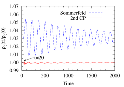
Figure 1: Radial oscillations of the central rest-mass density of a compact star in time. When Sommerfeld conditions are used a perturbation from the boundary (at $r_{\rm out}=20$) hits the center of the star (at $t=20$) and further perturbs it.

As an example of numerical artifact, pointed out but only briefly discussed in Bernuzzi and Hilditch (2010), we show in Fig. 1 the time evolution of the central rest-mass density of a equilibrium model of spherical compact star obtained with the Z4c formulation (coupled to general relativistic hydrodynamics equations) and two different BCs: Sommerfeld and CPBCs . The central density is expected to remain constant in time but the truncation error of the numerical scheme causes small oscillations around the initial value that converge away with resolution. This is clearly visible when CPBCs are used. The frequency of these oscillations corresponds to the proper radial mode of the star. When Sommerfeld conditions are used however the constraint violation at the boundary propagates into the domain and perturbs the star as soon as it becomes causally connected with the outer boundary. The perturbation from the boundary alters the mean value of the central density. The “boundary” perturbation does not converge (or converges much slower than the interior, see Sec. V.2) so becomes the dominant error when the grid is refined. At later times the oscillations are damped by the hydrodynamical interaction between the fluid and artificial vacuum, but the mean value of the central density is forever modified from the initial one. Such boundary artifacts can thus dramatically move the solution far away from the initial configuration in phase space, despite the fact that at late times the constraint violation is very small. Preliminary 3D simulations with the Jena BAM code Bruegmann et al. (2008) of single neutron stars, single puncture and binary black holes showed features very similar to the spherical results and in some cases instabilities triggered by the boundary.

In the following sections we discuss numerical results in spherical symmetry focusing only on the boundary conditions (60). Since the practical implementation of BCs in a code is also an issue, in Sec. V.1 we summarize the method we used as well as other standard approaches. We use the code of Bernuzzi and Hilditch (2010). For more information on our numerical method, spherical reduction of the equations please refer to appendix A of that reference. We perform several tests, in each case with Sommerfeld and constraint preserving conditions. To examine stability and the effect of the BCs we consider simulations with a very close outer boundary ($r_{\rm out}\simeq 20\,M$) and compare the results with a reference simulation Rinne et al. (2007); Ruiz et al. (2007), in which the outer boundary is placed far away ($r^{\prime}_{\rm out}\simeq 1000\,M$) from the origin. Since the boundary of the reference solution is causally disconnected on the time scale of the simulations with closer boundary, the BCs in the reference run have no importance. Results are presented for moderate resolution, about $\Delta r\sim 0.12$; but higher resolution runs as well as very long-term (hundreds of thousands of crossing times) simulations were performed showing the same behavior and no numerical instabilities. To monitor the global constraint violation we define the quantity:

$$C\equiv\sqrt{H^{2}+M^{i}M_{i}+\Theta^{2}+Z^{i}Z_{i}}\ ,$$ (118)

and we will refer to it as the constraint monitor. We will often make use of 2-norms of quantities:

$$||C(\cdot,t)||_{2}\equiv\sqrt{\int dr\,r^{2}C(r,t)^{2}}\ ,$$ (119)

where in practical computations the integral is performed on the grid by the trapezium rule. For a fair comparison with the “near-boundary” solution, the norm of the reference solution is taken only on the domain, $r\in(0,r_{\rm out})$.

Since most of the analytical results were obtained with the new asymptotically harmonic shift condition, we examine this gauge as well as the standard puncture gauge. In all cases we have found comparable results (see e.g. Fig. 4) and therefore we will focus primarily on the standard puncture gauge. We therefore aim to give at least some numerical evidence of well-posedness in those cases where we are unable to demonstrate strong mathematical results.

A brief description of the tests performed and their aim follows below.

Perturbed flat spacetime.

Evolution of constraint violating initial data on flat space. Here we focus on convergence and constraint absorption. We find near-perfect constraint transmission of the constraints when using the second order CPBCs. We devote the most attention to this test because the effect of the BCs are clearest in the absence of other sources of error.

Star spacetime.

Evolution of a stable compact star. In the Sommerfeld case, non convergent reflections from the boundary effect the dynamics of the star. The absorbing CPBCs completely solve this problem.

Black hole spacetime.

Evolution of black hole initial data. The robustness and performance of CPBCs are tested against black hole spacetimes with different initial data and gauges. In particular we evolve a single puncture and Schwarzschild with a Kerr-Schild slicing.

We use geometrical units $c=G=1$ everywhere, in case of matter spacetime dimensionless units are adopted setting $M_{\odot}=1$, in case of black hole spacetime $M_{\rm bh}=1$, while in case of flat spacetime a mass scale remains arbitrary.

V.1 Numerical implementation of boundary conditions

The literature contains many suggestions for the implementation of BCs, of which we highlight a small subset here.

Populate ghostzones.

One example is the recipe of Calabrese and Gundlach (2006), under which numerical stability of the shifted wave equation was proven. The idea is to write the BCs on the first order in time second order in space characteristic variables (which only implicitly contain time derivatives) and populate ghostzones so that the desired continuum boundary condition is satisfied. Ghostzones not determined by the BCs are simply populated by extrapolation. Since this method relies in an essential way on altering spatial derivatives locally, it is not clear how to apply the approach if one is computing spatial derivatives pseudo-spectrally. Furthermore the recipe may not give a unique prescription when one is given a system of equations.

Summation by parts.

As we have mentioned before, with the summation by parts schemes and penalty techniques a quantity that mirrors the continuum energy for a symmetric hyperbolic system is constructed on the discrete system. Since we do not rely on an energy (symmetric hyperbolicity) method in our well-posedness analysis we are not able to construct a summation by parts finite difference scheme that guarantees stability. Analysis and applications in numerical relativity can be found in Calabrese and Neilsen (2004); Calabrese et al. (2004); Lehner et al. (2005); Diener et al. (2007); Seiler et al. (2008); Taylor et al. (2010).

BCs as time derivatives of evolved fields.

The remaining approach we consider assumes that one may take spatial derivatives everywhere in a spatial slice. Inside a pseudo-spectral method spatial derivatives are naturally defined everywhere. On the other hand when approximating derivatives by finite differences, one may either use extrapolation to populate ghostzones, or take lop/one-sided differences near the boundary. The two methods are equivalent. To express the BCs on time derivatives of the metric one starts by substituting the definitions of the time-reduction variables (for example $\Theta,Z_{i}$ and $K_{ij}$) into the BCs. Then, if higher than first order time derivatives are still required, one may define a set of auxiliary reduction variables. One may use the equations of motion of the auxiliary variables in combination with the boundary conditions to eliminate spatial derivatives of auxiliary variables so that they may be confined to the boundary Bayliss and Turkill (1980); Novak and Bonazzola (2002). This approach was tested in the Caltech-Cornell SpEC code Rinne et al. (2009), but it is currently not used for binary black hole simulations. Here we perform evolutions only up to second order, and so do not need to use auxiliary variables in the boundary.

Our numerical tests are performed with a spherical reduction of the Z4c system. The numerical implementation of the boundary conditions in spherical symmetry is described in appendix C.

V.2 Perturbed flat spacetime

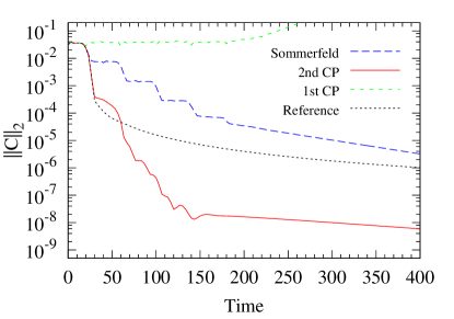
Figure 2: Constraint violation in flat spacetime test. The 2-norm of the constraint monitor is showed in time for different BCs implemented. The same quantity for the reference simulation is showed.

In this test an initial constraint violating Gaussian perturbation is prescribed in variable $\chi$. During the evolution it propagates, reaches the boundary and if completely absorbed, the system relaxes to the Minkowski solution. This does not happen in practice because reflections are always present. Here we investigate the magnitude of these reflections and compare CPBCs of 1st and 2nd order with standard Sommerfeld conditions.

Figure 2 shows the 2-norm of the constraint monitor in time, results from the reference simulation are also reported. All the data agree up to around $t=20$, i.e. when the solution is traveling through the grid. After that time the following happens: (i) the constraint violation remains almost constant for 1st order CPBCs (green dotted line) and eventually causes the simulation to crash; (ii) the constraint violation decreases for Sommerfeld (blue dashed line) initially not monotonically (notice the four plateaus) then, after $t=180$, reaching a monotonic behavior; (iii) the constraint violation for 2nd order CPBCs (continuous red line) is smaller than Sommerfeld, plateaus are less clear but a monotonic behavior is also reached after $t=180$; (iv) the reference solutions (black dotted line) agree among themselves (remember that on the plotted timescale the boundary of the reference solution is disconnected from the spatial domain under consideration) and decrease monotonically but in absolute value less than 2nd order CPBCs.

The interpretation of these observation is quite obvious, at least for points (i)-(iii): 1st order CPBCs simply do not absorb the perturbation, which is entirely reflected back; Sommerfeld BCs are affected by partial reflections and at each crossing time a smaller portion of the wave comes back into the domain until an almost complete absorption; 2nd order CPBCs immediately absorb the largest portion of the outgoing wave. These statements are quantified below.

Let us briefly discuss point (iv). A close look at the evolution of the constraint monitor in space shows a systematic drift from zero due to a back-scattering effect of the perturbation leaving the grid. This is responsible for the larger values of the constraint violation. Such an effect can not be simulated in the closer domain case because the CPBCs cut completely the incoming modes of the solution, and, effectively, two different numerical spacetimes are simulated in the two cases.

An important point is to quantify the absorption properties of the BCs under consideration. To this end we consider the characteristic fields associated to the $\Theta$ given by:

$$U^{\pm}_{\Theta}=\partial_{0}\Theta\pm\Theta_{,s}\ .$$ (120)

They can be regarded as incoming and outcoming modes of the solution. Thus we define an experimental reflection coefficient (inspired by Buchman and Sarbach (2006, 2007)) defined as the ratio of the Fourier modes of the characteristic fields at the boundary:

$$R\equiv\frac{|\tilde{U}^{-}_{\Theta}(k)|}{|\tilde{U}^{+}_{\Theta}(k)|}.$$ (121)

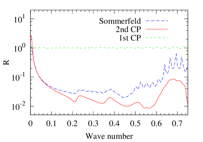
Figure 3: Experimental reflection coefficient in flat spacetime test. The experimental reflection coefficient, defined in Eq. (121), is plotted versus the wave number for different BCs implemented.

Figure 3 shows that $R\sim 1$ for 1st order CPBCs, while the behavior of 2nd order CPBCs is qualitatively similar to Sommerfeld. Since they do not absorb the constraint violation, in what follows, we discard the 1st order CPBCs.

The results presented so far refer to the puncture gauge. As stated at the beginning of the section, basically no significant differences are found when the asymptotically harmonic shift is employed. Figure 4 shows clearly this fact, we do not further comment on the asymptotically harmonic gauge until Sec. V.4.

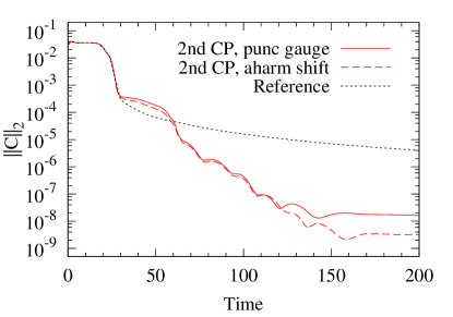
Figure 4: Constraint violation in flat spacetime test. Comparison of 2nd order CPBCs with puncture and asymptotically harmonic shift.

Finally, we present convergence results. In figure 5 the experimental self-convergence factor is plotted in time. While the physical solution is traveling on grid, $t<20$, the scheme is fourth order convergent as expected. Afterwards the numerical solution consists of the boundary reflections only and, while in case of Sommerfeld reflections are first order accurate, in case of CPBCs they maintain fourth order convergence up to $t\sim 100$. For later times (not shown in the plot) the absolute value of the solution (and of the reflections) is so small that only noise is seen. We remark that the order of extrapolation used to fill the ghosts points and the finite difference operators in the two approaches are the same, so the differences are really due only to BCs. In order to obtain these convergence results, a non-staggered grid must be used because the staggered grid converges to the continuum domain at only first order in the grid spacing. In the following applications we use staggered grids, since this is commonly done in 3D codes.

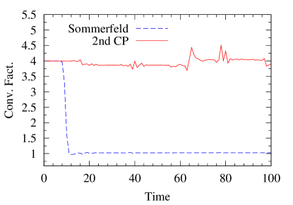
Figure 5: Convergence factor in flat spacetime test. The self-convergence factor is compute from the 2-norms of three simulations at different resolutions and showed in time for 2nd order CPBCs and Sommerfeld BCs.

V.3 Star spacetime

In this test we evolve stable spherical star initial data (see Bernuzzi and Hilditch (2010) for detail). At the beginning of the section we already discussed one of the main drawback of the use of Sommerfeld BCs with Z4c. As it is evident from Figure 1, the use of CPBCs is not optional but absolutely necessary to obtain reliable results. In a more complicated/dynamical scenario in fact such artifacts could be hidden or erroneously interpreted as real physics.

In this paper we are presenting results obtained without the Z4 constraint damping scheme Gundlach et al. (2005). One may however consider using the constraint damping scheme with a sufficiently large computational domain to suppress perturbations from the boundary. In our experience this is not only a inefficient cure (especially in 3D simulations) but an ineffective one. Our simulations indicate that the required damping coefficients are quite large, possibly because the perturbation from the boundary is typically not a high-frequency perturbation, and the damping scheme is most effective on high frequency perturbations. Constraint damping is analytically understood in the linear regime and high frequency approximation, in a more general situation the indiscriminate use of constraint damping may lead to undesirable effects (e.g. qualitatively similar to large artificial dissipation).

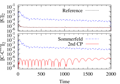
Figure 6: Constraint violation in star spacetime test. Upper panel: The 2-norm of the constraint monitor is plotted in time for different BCs implemented. The same quantity for the reference simulation is shown (black dotted line). Bottom panel: The 2-distance of the constraint monitor with the reference simulation is showed in time for different BCs implemented.

In the upper panel of Figure 6 we show the 2-norm of the constraint monitor for Sommerfeld, 2nd order CPBCs and the reference solution. It is evident that CPBCs are closer to the reference solution. In the bottom panel the distance from the reference solution is plotted showing that CPBCs lead to an improvement of approximately 2 to 4 orders of magnitude.

V.4 Black hole spacetime

In this test we consider different black hole spacetimes. A spherical black hole was evolved with puncture and Kerr-Schild initial data; evolutions were performed with both the gamma driver and asymptotically harmonic shift.

We focus first on the evolution of a single puncture. Figure 7 shows that the behavior of the constraint monitor, computed outside the apparent horizon, is analogous to what we found in the flat and star spacetime tests. As the solution asymptotes to the stationary trumpet slice Hannam et al. (2007) we find more constraint violation than in the evolution of the star. The resolution employed in the simulations for the figure is quite moderate and the outer boundary very close, even compared with a 3D code. Nonetheless the CPBCs perform quite well and significantly improve the numerical solution with respect Sommerfeld. No big differences were found when adopting either the gamma driver shift or the asymptotically harmonic one. As shown in Figure 8 the puncture shift (red solid line) does even better than the asymptotically harmonic (red dashed line) after $t\sim 60$. To the best knowledge of the authors this is the first time that the asymptotically harmonic shift has been used in the evolution of puncture data.

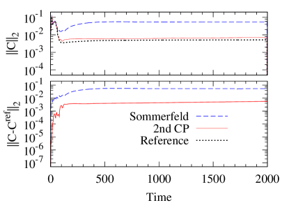
Figure 7: Constraint violation in black hole spacetime test. Upper panel: The 2-norm of the constraint monitor is showed in time for different BCs implemented. The same quantity for the reference simulation is showed (black dotted line). Bottom panel: The 2-distance of the constraint monitor with the reference simulation is showed in time for different BCs implemented.

To further assess the robustness of our BCs we evolve the spherical black hole with Kerr-Schild initial data:

$$ds^{2} =-\left(1-\frac{2M}{r}\right)\,dt^{2}+\frac{4M}{r}\,dt\,dr+\left(1+\frac{2M}{r}\right)\,dr^{2}$$

$$+r^{2}\,d\Omega^{2}\,.$$ (122)

The excision surface is at $r=1.9M$ and simple extrapolation is used at the inner boundary. We stress that this test is initially more demanding for the gamma driver shift. Since the line-element is not written in a manifestly conformally flat form, the shift immediately evolves everywhere in space, which is not the case with the gamma driver shift and puncture data. Figure 8 shows that the results for the constraint monitor obtained with our CPBCs are comparable to the puncture case with both the puncture shift (orange thick solid line) and the asymptotically harmonic (orange thick dashed line). In this case the latter perform better. Moreover, at this resolution, the bigger spurious reflections produced by Sommerfeld conditions combined with the close boundary used ($r^{\rm out}=20$) cause the simulations to crash. To achieve stable evolutions with the Sommerfeld conditions we find it necessary to use a higher resolution and a more distant outer boundary.

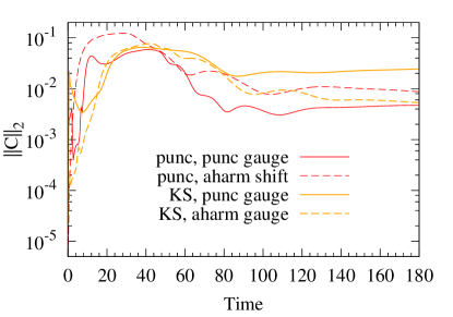
Figure 8: Constraint violation in black hole spacetime test, comparison of different initial data and gauges. The 2-norm of the constraint monitor is showed in time for 2nd order CPBCs. The evolutions refer to puncture initial data showed with puncture shift (red solid line) and asymptotically harmonic shift (red dashed line) and to Kerr-Schild initial data (evolved with excision) with puncture shift (thick orange solid line) and asymptotically harmonic shift (thick orange dashed line).

VI Conclusion

For numerical applications of free-evolution schemes in general relativity there is a strong motivation to construct constraint preserving boundary conditions. Without such conditions, constraint violations may appear at the boundary of the numerical domain and swamp the numerical solution. In the worst case such errors could be interpreted as real physics. In this study we have constructed constraint preserving conditions for the Z4c formulation of the Einstein equations with variations of the popular puncture gauge.

We demonstrated well-posedness of the resulting initial boundary value problem for the constraint subsystem on a four dimensional compact manifold in the high-frequency approximation. Since we are only interested in the constraint absorption properties of our boundary conditions we just analyzed the initial boundary value problem of the a spherical reduction of the Z4c system for a special choice of free parameters of the gauge condition. One may be able to expand our calculations for the asymptotically harmonic shift condition by verifying the existence of a suitable symmetrizer in a neighborhood of the point $p$ about which we perturb to reach the high-frequency limit. Unfortunately there is not a clear method for extending our calculations beyond the high-frequency limit with the standard gauge choice. Even in the high-frequency approximation we find that the Laplace-Fourier method becomes cumbersome. The key problem is that the cascade approach of Kreiss and Winicour fails with the puncture gauge.

In order to build a body of evidence for the well-posedness of the initial-boundary value problem with the standard puncture gauge we therefore performed numerical evolutions of various spherical initial data sets. Roughly speaking our approach for the implementation of the boundary conditions is to rewrite them as closely as possible to Sommerfeld conditions most commonly used in BSSN evolutions. We will report our method in detail elsewhere. Since the underlying formulation is not symmetric hyperbolic we are not able to make a summation-by-parts approach to the implementation. Therefore numerical stability is most straightforwardly established by studying toy problems mathematically and performing existence numerical tests on the numerical system. We compared the behavior of the system with the standard puncture gauge and the asymptotically harmonic gauge. We find very similar features in all tests. We demonstrated that with our approach to the numerical implementation we can achieve clean pointwise convergence even in reflected constraint violation. We also found, in agreement with previous studies, that high-order boundary conditions are able to absorb outgoing constraint violation much more effectively than first order conditions.

There are two obvious places in which we would like to strengthen our results. Firstly it is desirable to extend our well-posedness results, especially in the case of the standard puncture gauge. However in order to do this a different mathematical approach will probably be necessary. Secondly, that the numerical tests were performed in spherical symmetry is an obvious drawback which we aim to address shortly. Preliminary tests in 3D with the BAM code indicate that additional tangential terms in the boundary conditions, which we have discarded in this paper, are required in order to get a stable evolution.

Appendix A Well-Posed problems

The well-posedness of the IBVP is the requirement that for given initial and boundary data an unique solution should exist and it should depend continuously on the data (see e.g. Friedrich and Nagy (1999)). In this section we present a short review of the theory for first order systems to prove well-posedness This theory developed by Kreiss Kreiss (1970) gives us necessary and sufficient conditions for well-posedness of the IBVP for strictly hyperbolic systems. The theory was extended to hyperbolic systems of constant multiplicity by Agranovich Agranovich (1972). The discussion presented here follows closely that of in Kreiss (1970); Kreiss and Winicour (2006); Rinne (2006).

Consider a strongly hyperbolic system of equations of motion

$$\partial_{t}{u}={B}\,\partial_{x^{1}}u+\sum_{A=2}^{n}{C}^{A}\,\partial_{A}{u}\,,$$ (123)

with constant coefficients on the half-space $t\geq 0$, $x^{1}\geq 0$ and $-\infty<x^{2},\dots,x^{n}<\infty$. Here ${u}$ is a $n$-dimensional vector and ${B}$ and ${C}^{i}$ are $n\times n$ constant matrices. By assuming that ${B}$ is non-singular, it can be rewritten as

$${B}=\left(\begin{array}[]{cc}-{\Lambda}^{I}&0\\ 0&{\Lambda}^{II}\\ \end{array}\right)\,,$$ (124)

with ${\Lambda}^{I}$ and ${\Lambda}^{II}$ real and positive definite diagonal matrices of order $m$ and $n-m$ respectively. We imposed $m$ BCs at $x^{1}=0$ in the form

$$\left.{L}\,{u}^{I}(t,x)\right|_{x^{1}=0}\,\,\hat{=}\,\,{g}(t,x)\,,$$ (125)

where ${L}$ is a $m\times m$ constant matrix and $g={g}(t,x^{2},\dots,x^{n})$ is a given boundary data vector. For simplicity, we consider trivial initial data $u(0,x)=0$. In the following we solve the IBVP (123-125) by performing a Laplace-Fourier transformation with respect to the directions $t$ and $x^{A}$ tangential to the boundary $x^{1}=0$.

Let $\tilde{u}=\tilde{u}(s,x^{1},\omega^{A})$ denote the Laplace-Fourier transformation of $u(t,x)$. Then, $\tilde{u}$ satisfies the ordinary differential system

$$\partial_{x}\tilde{u}=M(s,\omega)\,\tilde{u}\,,\qquad\textrm{on}\,x\in(0,\infty)\,,$$ (126)

$${L}\tilde{{u}}^{I}\,\,\hat{=}\,\,\tilde{{g}}\,,\hskip 54.06006pt\textrm{at}\,x\,\,\hat{=}\,\,0\,,$$ (127)

where $\tilde{{g}}$ denotes the Laplace-Fourier transformation of $g$ and

$$M(s,\omega)=B^{-1}\,(s\,\mathbb{I}_{n\times n}+i\,\omega_{A}\,{C}^{A})\,.$$ (128)

If $\lambda_{i}$ and $e_{i}(s,\omega)$ are the corresponding eigenvalues and eigenvectors of $M$ then the general $L_{2}$ solution (functions which are quadratically integrable) of (126) is given by

$$\tilde{{u}}=\sum_{i=1}^{m}\sigma_{i}\,{e}_{i}(s,\omega)\,\,\textrm{exp}(\lambda_{i}\,x^{1})\,,$$ (129)

where $\sigma_{i}$ are complex integration constants . These constants are determined by the boundary conditions. By substituting (129) into the expression (127) we obtain a system of $m$ linear equations for the unknown $\sigma_{i}$. This system can be written in the form

$$\mathbb{D}(s,\omega)\,{\sigma}\,\,\hat{=}\,\,\tilde{{g}}\,,$$ (130)

where $\mathbb{D}(s,\omega)$ is a $m\times m$ matrix. Let us consider for a moment homogeneous BCs ${\tilde{g}}=0$ and suppose that there is $s$ with $\mbox{Re}(s)=\eta>0$ such that $\textrm{Det}\,\mathbb{D}=0$. It means that (130) has a non-trivial solution and therefore, the solution of the IBVP (123-125) is

$${u}(t,x^{i})=\tilde{{u}}(x^{1})\,\textrm{exp}\left(s\,t+i\,\omega_{A}\,x^{A}\right)\,.$$ (131)

This implies, by homogeneity of the system (126-127), that

$${u}(t,x^{i})=\tilde{{u}}(\theta\,x^{1})\,\textrm{exp}\left(\zeta\,s\,t+i\,\zeta\,\omega_{A}\,x^{A}\right)\,.$$ (132)

is also a solution for any constant $\zeta>0$. By increasing that constant arbitrarily one can find a solution which grows exponentially. Therefore, the IBVP is not well-posed. We conclude that the so-called determinant condition

$$\textrm{Det}\,\mathbb{D}\neq 0\,,\qquad\textrm{for}\qquad\eta>0\,,$$

is a necessary condition for well-posedness.

Next, let us consider the inhomogeneous BCs. Since the determinant condition is satisfied we can solve (130) for the integration constants. What remains to be shown is that solution (129) can be bounded in terms of the data given at the boundary,

$$|\tilde{{u}}(s,0,\omega)|\leq C\,|\tilde{{g}}(s,\omega)|\,,$$ (133)

where $C>0$ is an independent constant of $s$ and $\omega$. Using (133) and by inverting the Laplace-Fourier transformation it is possible to show that the estimate

$$\int_{0}^{T}\|u(t,\cdot)\|^{2}\,dt\leq\delta\int_{0}^{T}\left.\|g(t,\cdot)\|^{2}\right|_{x^{1}=0}\,dt\,,$$ (134)

holds, i.e. we can estimate the $L_{2}$ norm of the solution in terms of the $L_{2}$ norm of the given boundary data. Here the constant $\delta$ is independent of the boundary data. Systems whose solution (134) satisfies this estimate are called boundary stable Gustafsson et al. (1995); Kreiss (1970); Kreiss and Busenhart (2001).

Kreiss has shown in Kreiss (1970); Kreiss and Winicour (2006) that if the system (123) is strictly hyperbolic, the condition (133) implies that there is a symmetrizer ${H}={H}(s^{\prime},\omega^{\prime})$ such that

1. ${H}(s^{\prime},\omega^{\prime})$ is a smooth bounded function that depends of $(s^{\prime},\omega^{\prime})$,

2. there exists a constant $\delta>0$ such that

   $$H\,M+M^{*}\,H\geq\delta\,\eta\,\mathbb{I}\,,$$

   for all $\eta>0$ and all $\omega\in\mathbb{R}$,

3. there are constants $\delta_{2}>0$ and $C>0$ such that

   $$\left<\tilde{u},{H}\,\tilde{u}\right>\,\geq\delta_{2}|\tilde{u}|^{2}-C|\tilde{g}|^{2}\,,$$

   for all $\tilde{u}$ satisfying the boundary condition (130),

where $s^{\prime}=s/\kappa$, $\omega^{\prime}=\omega/\kappa$ and $\kappa=\sqrt{|s|^{2}+\omega^{2}}$ and $\omega^{2}={\omega_{y}^{2}+\omega_{z}^{2}}$. We have denoted the standard scalar product by $\left<,\,\cdot\,,\right>$ and $|\cdot|$ its corresponding norm. This symmetrizer allows us obtain an estimate of the solution of the system for which we add a source term $F(t,x)$ in the right of (123). In particular, according to Kreiss and Winicour (2006), we obtain an estimate of the form

$$\int_{0}^{T}\|{u}(t,\cdot)\|^{2}\,dt+\int_{0}^{T}\left\|{u}(t,\cdot)\|^{2}\right|_{x^{1}=0}\,dt\leq$$

$$\delta\,\left(\int_{0}^{T}\|{F}(t,\cdot)\|^{2}\,dt\,+\int_{0}^{T}\left.\|{g}(t,\cdot)\|^{2}\right|_{x^{1}=0}\,dt\right)\,,$$ (135)

where the constant $\delta>0$ is independent of the boundary data ${g}$ or the source term ${F}$.

Appendix B Toy Model

Consider the wave equation

$$\left[\partial^{2}_{0}-\mu^{2}\,\partial^{l}\partial_{l}\right]\,U\left(t,x^{i}\right)\,=\,F\left(t,x^{i}\right)\,,$$ (136)

on the half-space $t\geq 0$, $x\geq 0$ and $y$ and $z\in(-\infty,\infty)$ with trivial initial data. We impose BCs at $x\,\,\,\hat{=}\,\,\,0$ of the form

$$\left[\partial_{0}-\mu\,\partial_{x}\right]\,U(t,x^{i})\,\,\hat{=}\,\,h\,,$$ (137)

where $h$ are given boundary data and $\partial_{0}$ is the time derivative along the coordinate time in the linear regime.

According to Ruiz et al. (2007), let us denote to $\tilde{U}$ as the Laplace-Fourier transformation of $U(t,x^{i})$ with respect to the directions $t$, $y$ and $z$ tangential to the boundary then in the background (65), $\tilde{U}$ satisfies

$$\left[\left(\mu^{2}-\mathring{\beta}^{2}\right)\partial_{x}^{2}+2\,\mathring{\beta}\,s\,\partial_{x}-(s^{2}+\mu^{2}\,\omega^{2})\right]\tilde{U}=\tilde{F}\,,$$ (138)

$$\left[s-\left(\mu+\mathring{\beta}\right)\,\partial_{x}\right]\tilde{U}\,\,\hat{=}\,\,\tilde{h}\,,$$ (139)

where $\tilde{F}$ and $\tilde{h}$ denote the Laplace-Fourier transformations of $F$ and $h$ respectively. In order to apply the theory presented in the appendix A, one can rewrite the above system as a first order one by introducing the variable Ruiz et al. (2007); Kreiss and Winicour (2006)

$$D\tilde{U}=\frac{1}{\kappa}\,\left(\partial_{x}\tilde{U}+\gamma^{2}_{\mu}\,\mathring{\beta}\,s\,\tilde{U}\right)\,,$$ (140)

where $\gamma_{\mu}=1/\sqrt{\mu^{2}-\mathring{\beta}^{2}}$. Therefore, the system (138) can be rewritten in the form

$$\partial_{x}\tilde{W}=M(s,\omega)\,\tilde{W}+\tilde{f}\,,$$ (141)

$$L(s,\omega)\tilde{W}=\tilde{g}\,,$$ (142)

where we have defined

$$\tilde{W}=\left(\begin{array}[]{c}\tilde{U}\\ D\tilde{U}\end{array}\right)\,,\qquad\tilde{f}=\frac{\gamma_{\mu}^{2}}{\kappa}\left(\begin{array}[]{c}0\\ \tilde{F}\end{array}\right)\,,$$

and

$$M(s,\omega) = \kappa\,\left(\begin{array}[]{cc}-\gamma_{\mu}^{2}\,\mathring{\beta}\,s^{\prime}&1\\ \mu^{2}\,\gamma^{4}_{\mu}\,\lambda^{2}&-\gamma_{\mu}^{2}\,\mathring{\beta}\,s^{\prime}\end{array}\right)\,,$$ (145)

$$L(s,\omega) = (\mu\,s^{\prime},-\gamma^{-2}_{\mu})\,,$$ (146)

with $\lambda^{2}=s^{\prime 2}+\gamma^{-2}_{\mu}\,\omega^{\prime 2}$. The $L_{2}$ solution of the homogeneous system (141) is given by

$$\tilde{W}(s,x,\omega)=\sigma\,e^{(\tau^{-}x)}\,e^{-}\,.$$ (147)

where $\tau^{-}$ is the eigenvalue of $M$ with $\mbox{Re}(\tau^{-})<0$ and $e^{-}$ its corresponding eigenvector. Introducing (147) into the boundary we have

$$\mu\,\left(\,s^{\prime}+\sqrt{s^{\prime 2}+\gamma^{-2}_{\mu}\,\omega^{\prime 2}}\,\right)\sigma=\tilde{g}\,.$$ (148)

According to Kreiss and Winicour (2006); Ruiz et al. (2007), one can show that there is a constant $\delta>0$ such that

$$\left|s^{\prime}+\sqrt{s^{\prime 2}+\gamma^{-2}_{\mu}\,\omega^{\prime 2}}\,\right|\geq\delta\,.$$ (149)

Provided that the eigenvector $e^{-}$ in the solution (147) is normalized in a way that it remains finite as $\omega$ or $|s|$ goes to zero or infinity, there is a constant $C>0$ such that

$$|\tilde{W}(s,0,\omega,)|\leq\,C\,|\tilde{g}|\,,$$ (150)

for all $s\in\mathbb{C}$ with $\eta>0$, and $\omega\in\mathbb{R}$. Therefore, the system is boundary stable. So, we should consider the existence of a symmetrizer $H=H(s^{\prime},\omega^{\prime})$ and use it to get an energy estimate for the full problem. According to Ruiz et al. (2007), it can be shown that the following estimate

$$\eta\,\int\limits_{0}^{\infty}\left(|\kappa\,\tilde{U}|^{2}+|\partial_{x}\tilde{U}|^{2}\right)\,dx+\left.\left(|\kappa\,\tilde{U}|^{2}+|\partial_{x}\tilde{U}|^{2}\right)\right|_{x=0}$$ (151)

$$\leq C^{\prime}\,\left[\frac{1}{\eta}\,\int\limits_{0}^{\infty}\left|{\tilde{F}}\right|^{2}\,dx+\left|\tilde{h}\right|^{2}\right]\,,$$

holds for some constant $C^{\prime}>0$. Therefore, by inverting the Laplace-Fourier transformation and using the Parseval’s relation, one obtain the estimate (135) for the solution in terms of the $L_{2}$ norm of the boundary data.

One can generalize the boundary condition (137) to higher order BCs. It has been shown that such conditions reduce the amount of reflections at the boundary Buchman and Sarbach (2007); Rinne et al. (2009). Thus, we impose high order BCs of the form

$$\left[\partial_{0}-\mu\,\partial_{x}\right]^{m+1}\,U(t,x^{i})\,\,\hat{=}\,\,h\,,$$ (152)

with $m\geq 1$. Following Ruiz et al. (2007) it is possible rewrite the previous conditions as

$$\mathcal{L}^{m+1}\tilde{U}\,\,\hat{=}\,\,\left[\frac{\mu-\mathring{\beta}}{\kappa}\right]^{L+1}\,h\,,$$ (153)

where the linear operator $\mathcal{L}$ is defined by $\mathcal{L}=(\mu-\mathring{\beta})\,s^{\prime}-\partial_{x}/{\kappa\,\gamma_{\mu}^{2}}$. Using the equation of motion (141), we can rewrite the above condition in algebraic form. Note that

$$\mathcal{L}\left(\begin{array}[]{c}\tilde{U}\\ D\tilde{U}\end{array}\right)=A\,\left(\begin{array}[]{c}\tilde{U}\\ D\tilde{U}\end{array}\right)-\frac{1}{\kappa^{2}}\,\left(\begin{array}[]{c}0\\ \tilde{F}\end{array}\right)\,,$$ (154)

where the matrix $A$ is given by

$$A = \left(\begin{array}[]{cc}\mu\,\,s^{\prime}&-\gamma_{\mu}^{-2}\\ -\mu^{2}\,\gamma^{2}_{\mu}\,\lambda^{2}&\mu\,s^{\prime}\end{array}\right)\,.$$ (157)

It has been shown in Ruiz et al. (2007) that by iteration the boundary condition (153) can be rewritten in the form

$$L(s,\omega)=\frac{1}{2}\,\left(a_{+}^{m+1}+a_{-}^{m+1},-\,\frac{a_{+}^{m+1}-a_{-}^{m+1}}{\mu\,\lambda\,\gamma_{\mu}^{2}}\right)\,,$$ (158)

where $a_{\pm}=\mu\,(s^{\prime}\pm\lambda)$ are the eigenvalues of $A$. The $L_{2}$ solution of the homogeneous wave equation (141) is given by (147). Nevertheless, the integration constant $\sigma$ satisfies $a_{+}^{m+1}\,\sigma=\tilde{g}$. It can be shown that the system (141) with BCs (158) is boundary stable and, according to Ruiz et al. (2007), the solution satisfies the following estimate

$$\eta\,\int\limits_{0}^{\infty}\,\sum\limits_{j=0}^{m+1}\left|\kappa^{(m+1)-j}\,\partial_{x}^{j}\tilde{U}\right|^{2}\,dx+\left.\sum\limits_{j=0}^{m+1}\left|\kappa^{(m+1)-j}\,\partial_{x}^{j}\tilde{U}\right|^{2}\right|_{x=0}$$

$$\hskip 42.67912pt\leq C\left[\frac{1}{\eta}\,\int\limits_{0}^{\infty}\sum\limits_{j=0}^{m-1}\left|\kappa^{m-j}\partial_{x}^{j}\tilde{F}\right|^{2}\,dx\right.$$

$$\hskip 42.67912pt+\left.\left.\sum\limits_{j=0}^{m-1}\left|\kappa^{(m-1)-j}\partial_{x}^{j}\tilde{F}\right|^{2}\right|_{x=0}+\left|\tilde{h}\right|^{2}\right]\,,$$ (159)

for some strictly positive constant ${C}>0$. Thus, by inverting the Laplace-Fourier transformation we can estimate the $L_{2}$ norm of higher derivatives of the solution in terms of given data.

Appendix C Implementation of boundary conditions in spherical symmetry

In this appendix we describe the numerical implementation of the second order constraint preserving boundary conditions (60-62) in spherical symmetry.

We write the spherical line-element as

$$\textrm{d}s^{2}=\chi^{-1}\tilde{\gamma}_{rr}\textrm{d}r^{2}+\chi^{-1}\tilde{\gamma}_{T}r^{2}\textrm{d}\Omega^{2},$$ (160)

where $\textrm{d}\Omega^{2}=\textrm{d}\theta^{2}+\sin^{2}\theta\textrm{d}\phi^{2}$. Similarly we evolve $(\hat{K},\tilde{A}_{rr},\tilde{A}_{T})$ for the extrinsic curvature. In spherical symmetry the algebraic constraints (25) are

$$D=\log\left(\tilde{\gamma}_{rr}\tilde{\gamma}_{T}^{2}\right)=0, \quad T=\frac{\tilde{A}_{rr}}{\tilde{\gamma}_{rr}}+2\frac{\tilde{A}_{T}}{\tilde{\gamma}_{T}}=0.$$ (161)

Using the linearized equations of motion for the system, we rewrite the the boundary conditions as

$$\partial_{t}\Theta \,\,\hat{=}\,\,-\partial_{r}\Theta-\frac{1}{r}\Theta,$$ (162)

$$\partial_{t}\tilde{\Gamma}^{r} \,\,\hat{=}\,\,-\frac{2}{\sqrt{3}}\partial_{r}\tilde{\Gamma}^{r}-\frac{2}{\sqrt{3}r}\tilde{\Gamma}^{r}-\frac{4}{3r^{2}}\beta^{r}$$

$$-\frac{1}{3}\partial_{r}\Theta-\frac{2}{3}\partial_{r}\hat{K},$$ (163)

$$\partial_{t}\hat{K} \,\,\hat{=}\,\,-\sqrt{2}\,\partial_{r}\hat{K}-\frac{\sqrt{2}}{r}\,\hat{K}+\frac{1}{r}\,\partial_{r}\alpha,$$ (164)

$$\tilde{A}_{rr} \,\,\hat{=}\,\,-2\partial_{r}\tilde{A}_{rr}-\frac{6}{r}\tilde{A}_{rr}-\partial_{r}\partial_{r}\tilde{\gamma}_{T}-\frac{1}{2}\partial_{r}\tilde{\Gamma}^{r}$$

$$-\frac{2}{3}(-2+\sqrt{2})\partial_{r}\hat{K}+\frac{1}{3}\partial_{r}\Theta-\frac{2}{r^{2}}(\tilde{\gamma}_{rr}-\tilde{\gamma}_{T})$$

$$+\frac{1}{r}\big{(}\frac{5}{2}\partial_{r}\tilde{\gamma}_{rr}+2\partial_{r}\alpha-\frac{1}{3}\Theta-\frac{2\sqrt{2}}{3}\hat{K}-2\tilde{\Gamma}^{r}$$

$$-\partial_{r}\tilde{\gamma}_{T}-\partial_{r}\chi\big{)},$$ (165)

where here, for brevity, we have linearized around flat space. The boundary condition for $\tilde{A}_{T}$ can be obtained by using the algebraic constraints. Note the similarity with the Sommerfeld boundary condition. For the numerical implementation we populate ghostzones for each gridfunction $f_{i}$ by sixth order extrapolation

$$f_{N+i} =6f_{N+i-1}-15f_{N+i-2}+20f_{N+i-3}-15f_{N+i-4}$$

$$+6f_{N+i-5}-f_{N+i-6},$$ (166)

in order to approximate derivatives and compute Kreiss-Oliger artificial dissipation at the boundary. Here $N$ denotes the boundary point. For the variables $(\Theta,\tilde{\Gamma}^{r},\hat{K},\tilde{A}_{rr},\tilde{A}_{T})$ we simply replace the standard evolution equations with (162-165) at the boundary. The remaining variables are evolved according to their standard equation of motion at the boundary.

References

- Olsson (1995) P. Olsson, Mathematics of Computation 64, 1035 (1995).
- Gustafsson et al. (1995) B. Gustafsson, H. Kreiss, and J. Oliger, Time dependent problems and difference methods (Wiley, New York, 1995).
- Gundlach and Martin-Garcia (2004) C. Gundlach and J. M. Martin-Garcia, Phys. Rev. D70, 044032 (2004), eprint gr-qc/0403019.
- Nagy and Sarbach (2006) G. Nagy and O. Sarbach, Class. Quant. Grav. 23, S477 (2006), eprint gr-qc/0601124.
- Kreiss et al. (2009) H. O. Kreiss, O. Reula, O. Sarbach, and J. Winicour, Commun. Math. Phys. 289, 1099 (2009), eprint 0807.3207.
- Kreiss (1970) H. Kreiss, Commun. Pure Appl. Math. 23, 277 (1970).
- Agranovich (1972) M. Agranovich, Functional Anal. 6, 85 (1972).
- Taylor (1999) M. Taylor, Partial differential equation II, Qualitative Studies of Linear Equations (springer, New York, 1999), ISBN 10: 0387946543.
- Lehner et al. (2005) L. Lehner, O. Reula, and M. Tiglio, Class. Quant. Grav. 22, 5283 (2005), eprint gr-qc/0507004.
- M. Carpenter and Abarbanel (1994) D. G. M. Carpenter and S. Abarbanel, J. Comput. Phys. 111, 220 (1994).
- M. Carpenter and Gottlieb (1999) J. N. M. Carpenter and D. Gottlieb, J. Comput. Phys. 148, 341 (1999).
- Nordstrom and Carpenter (2001) J. Nordstrom and M. Carpenter, J. Comput. Phys. 173, 173 (2001).
- Friedrich (1985) H. Friedrich, Comm. Math. Phys. 100, 525 (1985).
- Friedrich (1996) H. Friedrich, Class. Quantum Grav. 13, 1451 (1996).
- Shibata and Nakamura (1995) M. Shibata and T. Nakamura, Phys. Rev. D 52, 5428 (1995).
- Baumgarte and Shapiro (1998) T. W. Baumgarte and S. L. Shapiro, Phys. Rev. D59, 024007 (1998), eprint gr-qc/9810065.
- Szilagyi and Winicour (2003) B. Szilagyi and J. Winicour, Phys. Rev. D68, 041501 (2003), eprint gr-qc/0205044.
- Lindblom et al. (2006) L. Lindblom, M. A. Scheel, L. E. Kidder, R. Owen, and O. Rinne, Class. Quant. Grav. 23, S447 (2006), eprint gr-qc/0512093.
- Kreiss and Winicour (2006) H. O. Kreiss and J. Winicour, Class. Quant. Grav. 23, S405 (2006), eprint gr-qc/0602051.
- Babiuc et al. (2006) M. C. Babiuc, B. Szilagyi, and J. Winicour, Phys. Rev. D73, 064017 (2006), eprint gr-qc/0601039.
- Motamed et al. (2006) M. Motamed, M. Babiuc, B. Szilagyi, and H.-O. Kreiss, Phys. Rev. D73, 124008 (2006), eprint gr-qc/0604010.
- Rinne (2006) O. Rinne, Class. Quant. Grav. 23, 6275 (2006), eprint gr-qc/0606053.
- Ruiz et al. (2007) M. Ruiz, O. Rinne, and O. Sarbach, Class. Quant. Grav. 24, 6349 (2007), eprint 0707.2797.
- Rinne et al. (2009) O. Rinne, L. T. Buchman, M. A. Scheel, and H. P. Pfeiffer, Class. Quant. Grav. 26, 075009 (2009), eprint 0811.3593.
- Campanelli et al. (2006) M. Campanelli, C. O. Lousto, P. Marronetti, and Y. Zlochower, Phys. Rev. Lett. 96, 111101 (2006), eprint gr-qc/0511048.
- Baker et al. (2006) J. G. Baker, J. Centrella, D.-I. Choi, M. Koppitz, and J. van Meter, Phys. Rev. Lett. 96, 111102 (2006), eprint gr-qc/0511103.
- Bruegmann et al. (2008) B. Bruegmann et al., Phys. Rev. D77, 024027 (2008), eprint gr-qc/0610128.
- Baiotti et al. (2008) L. Baiotti, B. Giacomazzo, and L. Rezzolla, Phys. Rev. D78, 084033 (2008), eprint 0804.0594.
- Tichy and Marronetti (2007) W. Tichy and P. Marronetti, Phys. Rev. D76, 061502 (2007), eprint gr-qc/0703075.
- Etienne et al. (2009) Z. B. Etienne, Y. T. Liu, S. L. Shapiro, and T. W. Baumgarte, Phys. Rev. D79, 044024 (2009), eprint 0812.2245.
- Hinder et al. (2010) I. Hinder, F. Herrmann, P. Laguna, and D. Shoemaker, Phys. Rev. D82, 024033 (2010), eprint 0806.1037.
- Shibata and Yoshino (2010) M. Shibata and H. Yoshino, Phys. Rev. D81, 021501 (2010), eprint 0912.3606.
- Nunez and Sarbach (2010) D. Nunez and O. Sarbach, Phys. Rev. D81, 044011 (2010), eprint 0910.5763.
- Bona et al. (2003) C. Bona, T. Ledvinka, C. Palenzuela, and M. Zacek, Phys. Rev. D67, 104005 (2003), eprint gr-qc/0302083.
- Bona et al. (2004) C. Bona, T. Ledvinka, C. Palenzuela, and M. Zacek, Phys. Rev. D69, 064036 (2004), eprint gr-qc/0307067.
- Gundlach et al. (2005) C. Gundlach, J. M. Martin-Garcia, G. Calabrese, and I. Hinder, Class. Quant. Grav. 22, 3767 (2005), eprint gr-qc/0504114.
- Bernuzzi and Hilditch (2010) S. Bernuzzi and D. Hilditch, Phys. Rev. D81, 084003 (2010), eprint 0912.2920.
- Bona et al. (2005) C. Bona, T. Ledvinka, C. Palenzuela-Luque, and M. Zacek, Class. Quant. Grav. 22, 2615 (2005), eprint gr-qc/0411110.
- Bona and Bona-Casas (2010) C. Bona and C. Bona-Casas, Phys. Rev. D 82, 064008 (2010).
- Alcubierre (2008) M. Alcubierre, Introduction to Numerical Relativity (Oxford Univ. Press, New York, 2008), ISBN 978-0-19-920567-7.
- Mueller et al. (2010) D. Mueller, J. Grigsby, and B. Brúgmann (2010), eprint gr-qc/10034681.
- Lousto and Zlochower (2010) C. O. Lousto and Y. Zlochower (2010), eprint gr-qc/10090292.
- Hilditch and Richter (2010) D. Hilditch and R. Richter (2010), eprint gr-gc/10024119.
- Nagy et al. (2004) G. Nagy, O. E. Ortiz, and O. A. Reula, Phys. Rev. D70, 044012 (2004), eprint gr-qc/0402123.
- Bayliss and Turkill (1980) A. Bayliss and E. Turkill, Comm. Pure and Appl. Math. 33, 707 (1980).
- Buchman and Sarbach (2006) L. T. Buchman and O. C. A. Sarbach, Class. Quant. Grav. 23, 6709 (2006), eprint gr-qc/0608051.
- Kreiss and Busenhart (2001) H. O. Kreiss and H. U. Busenhart, Time-Dependent Partial Differential Equations and Their Numerical Solution (Lectures in Mathematicas ETH, Zürich, 2001).
- Hilditch and Ruiz (2010) D. Hilditch and M. Ruiz (2010), in preparation.
- Buchman and Sarbach (2007) L. T. Buchman and O. C. A. Sarbach, Class. Quant. Grav. 24, S307 (2007), eprint gr-qc/0703129.
- Not (a) In Bernuzzi and Hilditch (2010) maximally dissipative conditions were used to cure the problem, CPBCs are the natural extension.
- Rinne et al. (2007) O. Rinne, L. Lindblom, and M. A. Scheel, Class. Quant. Grav. 24, 4053 (2007), eprint 0704.0782.
- Calabrese and Gundlach (2006) G. Calabrese and C. Gundlach, Class. Quant. Grav. 23, S343 (2006), eprint gr-qc/0509119.
- Calabrese and Neilsen (2004) G. Calabrese and D. Neilsen, Phys. Rev. D69, 044020 (2004), eprint gr-qc/0308008.
- Calabrese et al. (2004) G. Calabrese, L. Lehner, O. Reula, O. Sarbach, and M. Tiglio, Class. Quant. Grav. 21, 5735 (2004), eprint gr-qc/0308007.
- Diener et al. (2007) P. Diener, E. N. Dorband, E. Schnetter, and M. Tiglio, J. Sci. Comput. 32, 109 (2007), eprint gr-qc/0512001.
- Seiler et al. (2008) J. Seiler, B. Szilagyi, D. Pollney, and L. Rezzolla, Class. Quant. Grav. 25, 175020 (2008), eprint 0802.3341.
- Taylor et al. (2010) N. W. Taylor, L. E. Kidder, and S. A. Teukolsky, Phys. Rev. D82, 024037 (2010), eprint 1005.2922.
- Novak and Bonazzola (2002) J. Novak and S. Bonazzola (2002), eprint gr-qc/0203102.
- Hannam et al. (2007) M. Hannam, S. Husa, D. Pollney, B. Bruegmann, and N. O’Murchadha, Phys. Rev. Lett. 99, 241102 (2007), eprint gr-qc/0606099.
- Friedrich and Nagy (1999) H. Friedrich and G. Nagy, Comm. Math. Phys. 201, 619 (1999).
- Not (b) If the matrix does not have a complete set of eigenvectors then the integration constants have to be replaced with polynomials in .