Detecting gravitational waves from precessing binaries of spinning compact objects: Adiabatic limit

Abstract

Black-hole (BH) binaries with single-BH masses $m=5\mbox{--}20M_{\odot}$, moving on quasicircular orbits, are among the most promising sources for first-generation ground-based gravitational-wave (GW) detectors. Until now, the development of data-analysis techniques to detect GWs from these sources has been focused mostly on nonspinning BHs. The data-analysis problem for the spinning case is complicated by the necessity to model the precession-induced modulations of the GW signal, and by the large number of parameters needed to characterize the system, including the initial directions of the spins, and the position and orientation of the binary with respect to the GW detector. In this paper we consider binaries of maximally spinning BHs, and we work in the adiabatic-inspiral regime to build families of modulated detection templates that (i) are functions of very few physical and phenomenological parameters, (ii) model remarkably well the dynamical and precessional effects on the GW signal, with fitting factors on average $\gtrsim 0.97$, but (iii) might require increasing the detection thresholds, offsetting at least partially the gains in the fitting factors. Our detection-template families are quite promising also for the case of neutron-star–black-hole binaries, with fitting factors on average $\approx 0.93$. For these binaries we also suggest (but do not test) a further template family, which would produce essentially exact waveforms written directly in terms of the physical spin parameters.

I Introduction

A world-wide network of laser-interferometer gravitational-wave (GW) detectors, recently built Inter , has by now begun operation. Inspiraling binaries of compact objects, such as black holes (BHs) and neutron stars (NSs) are among the most promising astrophysical sources for these detectors. The GWs from the inspirals are expected to enter the frequency band of good detector sensitivity during the last few seconds or minutes of evolution of the binaries; GW scientists plan to track the phase of the signals very accurately, and to enhance the signal-to-noise ratio by integrating the signals coherently over their duration in the detector band. This is achieved by filtering the detector output with a bank of templates that represent our best theoretical predictions for the signals.

Until now, the development of data-analysis techniques has been focused mostly on binaries containing NSs (whose spins are negligible for data-detection purposes) and nonspinning BHs DA . Nonspinning, high-mass BHs pose a delicate problem: the breakdown of the post–Newtonian (PN) expansion in the last stages of the inspiral makes it hard to prepare reliable templates for the detection of binary BHs (BBHs) of relatively high total mass (say, $10\mbox{--}40M_{\odot}$) with LIGO–VIRGO interferometers. Various resummation techniques, such as Padé approximants DIS1 and Effective One-Body (EOB) techniques BD ; EOB3PN have been developed to extend the validity of PN formalism PN . Damour, Iyer, and Sathyaprakash DIS3 compared the templates generated by different PN treatments, and found that they can be very different. In a companion paper to the present one (BCV1, , henceforth BCV1), we investigated this issue for the GW signals emitted by comparable-mass BBHs with a total mass $M=10\mbox{--}40M_{\odot}$. In BCV1 we proposed a few examples of detection template families (DTFs), built either as time series or directly in the frequency domain, which try to address the failure of the PN expansion. The philosophy behind DTFs is to replace a family of signals that correspond to a specific mathematical model of the binary with families that can cover a broader range of plausible signals. Because the direct correspondence with the mathematical model is lost, DTFs are appropriate for the purpose of first detecting GW signals, but do not give direct estimates of physical parameters, such as the masses of the binary constituents. [Within the EOB framework, see also the recent paper by Damour, Iyer, Jaranowski, and Sathyaprakash DIJS , where the authors extend 3PN EOB templates with seven flexibility parameters and then show that the unextended 3PN templates already span the ranges of the flexibility parameters consistent with plausible 4PN effects.]

Very little is known about the statistical distribution of spins for the BHs in binaries: the spins could very well be large. Apostolatos, Cutler, Sussman, and Thorne (ACST94, ; apostolatos2, , henceforth ACST) have shown that when this is the case, the evolution of the GW phase and amplitude during the inspiral will be significantly affected by spin-induced modulations and irregularities. In a BBH, these effects can become dramatic if the two spins are large and they are not exactly aligned or antialigned with the orbital angular momentum. If this happens, there is a considerable chance that the analysis of interferometer data, carried out without taking spin effects into accounts, could miss the signals from these spinning BBHs altogether. The gravitational waveforms from binaries of spinning compact objects depend on many parameters: the masses and spins of the objects, the angles that describe the relative orientations of detector and binary, and the direction of propagation of GWs to the detector. In practice it is impossible, due to the extremely high computational cost, to filter the signals with a template bank parametrized by all of these parameters. One strategy is that of providing effective templates that depend on fewer parameters, but that have still reasonably high overlaps with the expected physical signals. An interesting suggestion, built on the results obtained in Ref. ACST94 , came from Apostolatos apostolatos2 , who introduced a modulational sinusoidal term in the frequency-domain phase of the templates to capture the effects of precession. However, while Apostolatos’ family reduces the number of parameters considerably, its computational requirements are still very high. Moreover, using an approximated analytical model of NS–BH waveforms, Grandclément, Kalogera and Vecchio GKV showed that this family fails to capture those waveforms satisfactorily (see however Ref. GK for a hierarchical scheme that can improve the fit by adding “spikes?? in the template phasing).

In this paper, complementary to BCV1, we study the data analysis of GWs from binaries with spinning BHs; for simplicity, we restrict our analysis to the adiabatic limit, where the two compact objects in the binary (either two BHs, or a NS and a BH) follow an adiabatic sequence of spherical orbits driven by radiation reaction (RR). The denomination of spherical orbits comes from the fact that the orbital plane is not fixed in space, but precesses, so the orbits trace a complicated path on a (slowly shrinking) spherical surface. We neglect the problems caused by the failure of PN expansion in these binaries (note that the conservative part of the EOB framework BD has already been extended to the spinning case by Damour TD , providing a tool to move beyond the adiabatic approximation; we plan to add radiation-reaction effects to this model, and to study the consequences on GW emission and detection elsewhere). Here, we carry out a detailed study of PN precessional dynamics and of GW generation in precessing binaries in the adiabatic limit, and we use the resulting insights to build a new class of modulated effective templates where modulational effects are introduced in both the frequency-domain amplitude and frequency-domain phase of the templates. The mathematical structure of our templates suggests a way to search automatically over several of the parameters (in strict analogy to the automatic search over initial template phase in the data analysis of nonspinning binaries), reducing computational costs significantly. We argue that our families should capture very well the expected physical signals.

We note here a shift in perspective from BCV1. In this paper, we use the PN equations for the two-body dynamics of spinning compact objects to build a fiducial model (our target model) that represents our best knowledge of the expected physical signals. Because we cannot use the target model directly for data analysis (it has too many parameters), we build effective template families with fewer parameters. These families are then compared with the target model for a variety of binary parameters, to gauge their ability to match the physical signals (their effectualness DIS1 ). On the other hand, in BCV1 we employed several variants of the PN equations (with diverging behaviors in the late phase of inspiral) to identify a range of plausible physical signals; we then built our DTFs so that they would match all of the PN target models satisfactorily. This said, we shall still refer to the template families developed in the present paper as DTFs. We direct the reader to BCV1 for a simple introduction to matched-filtering techniques and their use in GW data analysis (developed in the literature by various authors DA ; DIS1 ; DIS3 ), and for an explanation of some of the notation used in this paper.

This paper is organized as follows. In Sec. II we define the target model, and we explain the conventions used to represent the generation and propagation of GWs. In Sec. III we study the two-body dynamics of spinning compact objects, looking for the features that are especially relevant to the data-analysis problem. Using this insight, in Sec. IV we formulate our DTFs, and we also describe two families of standard stationary-phase–approximation (SPA) templates, to be used as a comparison when evaluating the performance of the DTFs. In Sec. V we discuss the overlap and false-alarm statistics of our DTFs. In Sec. VI we evaluate the performance of our DTFs for BBHs and NS–BH binaries, and we briefly discuss a more advanced (and very promising) template family for NS–BH systems. In Sec. VII we summarize our conclusions.

Throughout this paper we adopt the noise spectral density for LIGO-I given by Eq. (28) of BCV1. The projected VIRGO noise curve is quite different (deeper at low frequencies, with a displaced peak-sensitivity frequency). So our results for high-mass binaries cannot be applied naively to VIRGO. We plan to repeat this study for VIRGO in the near future.

II Definition of the target model

In this section we define the target model used in this paper as a fiducial representation of the GW signals expected from precessing binaries of spinning compact objects. We restrict our analysis to the adiabatic regime where the inspiral of the compact objects can be represented as a sequence of quasicircular orbits. At any point along the inspiral, a binary of total mass $M=m_{1}+m_{2}$ and symmetric mass ratio $\eta=m_{1}m_{2}/M^{2}$ is completely described by the orbital angular frequency $\omega$, the orbital phase $\Psi$, the direction $\hat{\mathbf{L}}_{N}\propto\mathbf{r}\times\mathbf{v}$ of the orbital angular momentum, and the two spins $\mathbf{S}_{1}=\chi_{1}m_{1}^{2}\hat{\mathbf{S}}_{1}$ and $\mathbf{S}_{2}=\chi_{2}m_{2}^{2}\hat{\mathbf{S}}_{2}$, where $\hat{\mathbf{S}}_{1,2}$ are unit vectors and $0<\chi_{1,2}<1$. Throughout this paper we shall use carets to denote unit vectors, and we shall adopt geometrical units.

In Sec. II.1 we write the PN equations that govern the adiabatic evolution of the binary and the precession of $\hat{\mathbf{L}}_{N}$ and of $\mathbf{S}_{1,2}$. All the target waveforms used to test the effectualness DIS1 of our DTFs are obtained by integrating these equations numerically. The validity of the adiabatic approximation is discussed in App. A. In Sec. II.2 we discuss our criterion for stopping the numerical integration of the evolution equations at the point where the adiabatic approximation ceases to be valid. In Sec. II.3, building on Refs. FC ; ACST94 ; K , we describe a formalism for computing the response of a ground-based detector to the GWs generated by a spinning binary; the response is not just a function of the trajectory of the binary, but also of the relative direction and orientation of binary and detector. The formalism describes also how the precession of the binary modulates the detector response. Last, in Sec. II.4 we give a classification of all the parameters that enter the expression for the detector response, distinguishing those that specify the evolution of the binary itself from those that describe the relative direction and orientation of binary and detector.

II.1 Equations for an adiabatic sequence of precessing spherical orbits

The path of the binary across the sequence of quasicircular orbits is described by the adiabatic evolution of the orbital angular frequency $\omega$ up to 3.5PN order [2PN, ; BIWW, ; 2.5PNand3.5PN, ; BFIJ, ,DIS3, ] with spin effects included up to 2PN order [KWW, ,2PN, ,K, ],

$$\frac{\dot{\omega}}{\omega^{2}}=\frac{96}{5}\,\eta\,(M\omega)^{5/3}\Bigg{\{}1-\frac{743+924\,\eta}{336}\,(M\omega)^{2/3}-\Bigg{(}\frac{1}{12}\sum_{i=1,2}\bigg{[}\chi_{i}\left(\hat{\mathbf{L}}_{N}\cdot\hat{\mathbf{S}}_{i}\right)\left(113\frac{m_{i}^{2}}{M^{2}}+75\eta\right)\bigg{]}-4\pi\Bigg{)}(M\omega)$$

$$+\Bigg{(}\frac{34\,103}{18\,144}+\frac{13\,661}{2\,016}\,\eta+\frac{59}{18}\,\eta^{2}\Bigg{)}\,(M\omega)^{4/3}-\frac{1}{48}\eta\chi_{1}\chi_{2}\left[247(\hat{\mathbf{S}}_{1}\cdot\hat{\mathbf{S}}_{2})-721(\hat{\mathbf{L}}_{N}\cdot\hat{\mathbf{S}}_{1})(\hat{\mathbf{L}}_{N}\cdot\hat{\mathbf{S}}_{2})\right]\,(M\omega)^{4/3}$$

$$-\frac{1}{672}\,(4\,159+15\,876\,\eta)\,\pi\,(M\omega)^{5/3}+\Bigg{[}\left(\frac{16\,447\,322\,263}{139\,708\,800}-\frac{1\,712}{105}\gamma_{E}+\frac{16}{3}\pi^{2}\right)+\left(-\frac{273\,811\,877}{1\,088\,640}+\frac{451}{48}\pi^{2}-\frac{88}{3}\hat{\theta}\right)\eta$$

$$+\frac{541}{896}\eta^{2}-\frac{5\,605}{2\,592}\eta^{3}-\frac{856}{105}\log\left[16(M\omega)^{2/3}\right]\Bigg{]}(M\omega)^{2}+\Bigg{(}-\frac{4\,415}{4\,032}+\frac{358\,675}{6\,048}\,\eta+\frac{91\,495}{1\,512}\,\eta^{2}\Bigg{)}\,\pi\,(M\omega)^{7/3}\Bigg{\}}\,,$$ (1)

where $\gamma_{E}=0.577\ldots$ is Euler’s constant, and where $\hat{\theta}$ is an arbitrary parameter that enters the GW flux at 3PN order BFIJ and that could not be fixed in the regularization scheme used by the authors of Ref. BFIJ . Note that in Eq. (1) we set the static parameter $\omega_{s}=0$ DJSd . (Note for v4 of this paper on gr-qc: Eq. (1) is now revised as per Ref. errata ; the parameter $\hat{\theta}$ has been determined to be 1039/4620 thetapar .) The precession equations for the two spins are (see, for instance, Eqs. (4.17b,c) of Ref. K or Eqs. (11b,c) of Ref. ACST94 )

$$\dot{\mathbf{S}}_{1} = \frac{(M\omega)^{2}}{2M}\left\{\eta\,(M\omega)^{-1/3}\,\left(4+3\frac{m_{2}}{m_{1}}\right)\hat{\mathbf{L}}_{N}+\frac{1}{M^{2}}\,\left[\mathbf{S}_{2}-3(\mathbf{S}_{2}\cdot\hat{\mathbf{L}}_{N})\hat{\mathbf{L}}_{N}\right]\right\}\times\mathbf{S}_{1}\,,$$ (2)

$$\dot{\mathbf{S}}_{2} = \frac{(M\omega)^{2}}{2M}\left\{\eta\,(M\omega)^{-1/3}\left(4+3\frac{m_{1}}{m_{2}}\right)\hat{\mathbf{L}}_{N}+\frac{1}{M^{2}}\,\left[\mathbf{S}_{1}-3(\mathbf{S}_{1}\cdot\hat{\mathbf{L}}_{N})\hat{\mathbf{L}}_{N}\right]\right\}\times\mathbf{S}_{2}\,,$$ (3)

where we have replaced $r$ and $|\mathbf{L}_{N}|$ by their leading-order Newtonian expressions in $\omega$,

$$r=\left(\frac{M}{\omega^{2}}\right)^{1/3}\,,\quad\quad|\mathbf{L}_{N}|=\mu\,r^{2}\omega=\eta\,M^{5/3}\omega^{-1/3}\,.$$ (4)

This approximation is appropriate because the next spin-precession term is ${\cal O}(\omega^{1/3})$ higher than the leading order, while next terms in the expressions of $r$ and $|\mathbf{L}_{N}|$ are ${\cal O}(\omega^{2/3})$ higher.

The precession of the orbital plane (defined by the normal vector $\hat{\mathbf{L}}_{N}$) can be computed as follows. From Eqs. (4.7) and (4.11) of Ref. K we see that the total angular momentum $\mathbf{J}$ and its rate of change $\dot{\mathbf{J}}_{\rm RR}$ (due to RR) depend on $\omega$, $\hat{\mathbf{L}}_{\mathrm{N}}$ and $\mathbf{S}_{1,2}$ (schematically) as ($\mathbf{S}=\mathbf{S}_{1}+\mathbf{S}_{2}$)

$$\mathbf{J}=\mathbf{L}+\mathbf{S}=\underbrace{\eta\,M^{2}\,(M\omega)^{-1/3}\,\hat{\mathbf{L}}_{\mathrm{N}}\,\left[1+{\cal O}(\omega^{2/3})\right]-\eta\,(M\omega)^{2/3}\,\mathbf{S}_{\rm eff}}_{\mathbf{L}}+\mathbf{S}\,,$$ (5)

$$\dot{\mathbf{J}}_{\rm RR}=-\frac{32}{5}\eta^{2}M(M\omega)^{7/3}\,\hat{\mathbf{L}}_{N}\left[1+{\cal O}(\omega^{2/3})\right]+{\cal O}(\omega^{10/3})\,\hat{\mathbf{S}}_{1}+{\cal O}(\omega^{10/3})\,\hat{\mathbf{S}}_{2}\,,$$ (6)

where the combination

$$\mathbf{S}_{\rm eff}\equiv\left(1+\frac{3}{4}\,\frac{m_{2}}{m_{1}}\right)\,\mathbf{S}_{1}+\left(1+\frac{3}{4}\,\frac{m_{1}}{m_{2}}\right)\,\mathbf{S}_{2}$$ (7)

is known as effective spin TD . Note that both terms in the $\mathbf{L}$ brace of Eq. (5) originate from orbital angular momentum (the second term comes from the spin-orbit coupling). Taking the time derivative of (5), we obtain

$$\dot{\mathbf{J}}=\eta\,M^{2}\,(M\omega)^{-1/3}\,\dot{\hat{\mathbf{L}}}_{\rm N}\left[1+{\cal O}(\omega^{2/3})\right]-{\cal O}(\omega^{2/3})\,\dot{\mathbf{S}}_{\rm eff}+\dot{\mathbf{S}}+\left[{\cal O}(\omega^{7/3})\,\hat{\mathbf{L}}_{\mathrm{N}}-{\cal O}(\omega^{10/3})\,\mathbf{S}_{\rm eff}\right]\,,$$ (8)

where to get the last term on the right-hand side we have used $\dot{\omega}={\cal O}(\omega^{11/3})$. Comparing Eqs. (8) and (6), projecting out only the direction perpendicular to $\hat{\mathbf{L}}_{\mathrm{N}}$, and keeping only the terms up to the leading and next-to-leading orders, we get

$$\dot{\hat{\mathbf{L}}}_{N}=-\frac{(M\omega)^{1/3}}{\eta M^{2}}\,\dot{\mathbf{S}}=\frac{\omega^{2}}{2M}\Bigg{\{} \!\!\!\!\!\!\left[\left(4+3\frac{m_{2}}{m_{1}}\right)\,\mathbf{S}_{1}+\left(4+3\frac{m_{1}}{m_{2}}\right)\,\mathbf{S}_{2}\right]\times\hat{\mathbf{L}}_{N}$$ (9)

$$\!\!\!\!\!\!-\frac{3\,\omega^{1/3}}{\eta\,M^{5/3}}\left[(\mathbf{S}_{2}\cdot\hat{\mathbf{L}}_{N})\,\mathbf{S}_{1}+(\mathbf{S}_{1}\cdot\hat{\mathbf{L}}_{N})\,\mathbf{S}_{2}\right]\times\hat{\mathbf{L}}_{N}\Bigg{\}}\,.$$

Thus, we now have the set of four equations (1)–(3) and (9) for the four variables $\omega$, $\mathbf{S}_{1}$, $\mathbf{S}_{2}$, and $\hat{\mathbf{L}}_{N}$. We follow Ref. K , Eq. (4.15), in defining the accumulated orbital phase $\Psi$ as

$$\Psi\equiv\int_{t_{i}}^{t}\omega\,dt=\int_{\omega_{i}}^{\omega}\,\frac{\omega}{\dot{\omega}}\,d\omega\,.$$ (10)

This phase describes the position of the two compact objects along the instantaneous circular orbits of the adiabatic sequence; the phase of the GW waveforms, as detected by a ground-based detectors, differs from this by precessional effects, as explained below in Sec. II.3.

II.2 Endpoint of evolution

The orbital energy of the two-body system at 2PN and 3PN orders, expressed as a function of $\omega$, and assuming the static parameter $\omega_{s}=0$ DJS ; DJSd , reads [2PN, ,KWW, ,BFIJ, ]

$$E_{\rm 2PN}(\omega) = -\frac{\mu}{2}\,(M\omega)^{2/3}\,\left\{1-\frac{(9+\eta)}{12}\,(M\omega)^{2/3}+\frac{8}{3}\hat{\mathbf{L}}_{N}\cdot\frac{\mathbf{S}_{\rm eff}}{M^{2}}\,(M\omega)+\frac{1}{24}(-81+57\eta-\eta^{2})\,(M\omega)^{4/3}\right.$$ (11)

$$\left.+\frac{1}{\eta}\,\left[\frac{\mathbf{S}_{1}}{M^{2}}\cdot\frac{\mathbf{S}_{2}}{M^{2}}-3\left(\hat{\mathbf{L}}_{N}\cdot\frac{\mathbf{S}_{1}}{M^{2}}\right)\left(\hat{\mathbf{L}}_{N}\cdot\frac{\mathbf{S}_{2}}{M^{2}}\right)\right]\,(M\omega)^{4/3}\right\}\,,$$

$$E_{\rm 3PN}(\omega) = E_{\rm 2PN}(\omega)-\frac{\mu}{2}\,(M\omega)^{2/3}\,\left\{\left[-\frac{675}{64}+\left(\frac{34445}{576}-\frac{205}{96}\pi^{2}\right)\eta-\frac{155}{96}\eta^{2}-\frac{35}{5184}\eta^{3}\right]\,(M\omega)^{2}\right\}\,.$$ (12)

In the context of our adiabatic approximation, it is natural to stop the integration of Eqs. (1)–(3) and (9) at the point (the Minimum Energy Circular Orbit, or MECO) where the energy $E_{n\rm PN}$ reaches a minimum,

$${\rm MECO:}\quad\frac{dE_{n\rm PN}}{d\omega}=0\,;$$ (13)

after this point the adiabatic approximation breaks down note37 . (The MECO is discussed by Blanchet LB for nonspinning binaries under the name ICO, for Innermost Circular Orbit.) However, if we find that $\dot{\omega}=0$ (which implies certainly that the adiabatic approximation has become invalid) before the MECO is reached, we stop the evolution there. In BCV1 we noticed that for nonspinning binaries this behavior occurs for the 2.5PN evolutions, but not at 2PN, 3PN and 3.5PN orders.

Throughout this paper, we shall call the instantaneous frequency of GWs at the endpoint of evolution the ending frequency, which, up to a correction that arises from precessional effects, is twice the instantaneous orbital frequency defined in this section. It so happens (see BCV1) that a knowledge of the ending frequency is important to cut off the candidate detection templates at the point where we know too little about the physical signals to model them further. In Sec. III.2 we study the dependence of the ending frequency on the spins of the binary.

II.3 Gravitational waveforms

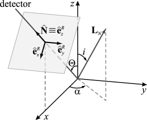
Figure 1: Source and radiation frames in the FC convention FC .

As we have seen, the trajectory of the inspiraling binary is obtained by integrating Eqs. (1)–(3) and (9) for the time evolution of $\omega(t)$, $\mathbf{S}_{1}(t)$, $\mathbf{S}_{2}(t)$ and $\hat{\mathbf{L}}_{N}(t)$. To determine the corresponding gravitational waveforms, we need to choose a specific coordinate system. We follow the convention proposed by Finn and Chernoff (FC, , henceforth FC), and also adopted by Kidder K . FC employ a fixed (source) coordinate system with unit vectors $\{\mathbf{e}_{x}^{S}$, $\mathbf{e}_{y}^{S}$, $\mathbf{e}_{z}^{S}\}$ (see Fig. 1). For a circular orbit, the leading-order mass-quadrupole waveform is (throughout this paper, we use geometrical units)

$$h^{ij}=\frac{2\mu}{D}\,\left(\frac{M}{r}\right)\,Q_{c}^{ij}\,,$$ (14)

where $D$ is the distance between the source and the Earth, and where $Q_{c}^{ij}$ is proportional to the second time derivative of the mass-quadrupole moment of the binary,

$$Q_{c}^{ij}=2\left[\lambda^{i}\,\lambda^{j}-n^{i}\,n^{j}\right]\,,$$ (15)

with $n^{i}$ and $\lambda^{i}$ the unit vectors along the separation vector of the binary $\mathbf{r}$ and along the corresponding relative velocity $\mathbf{v}$. These unit vectors are related to the adiabatic evolution of the dynamical variables by

$$\hat{\mathbf{n}}=\mathbf{e}_{1}^{S}\,\cos\Phi_{S}+\mathbf{e}_{2}^{S}\,\sin\Phi_{S}\,,\quad\hat{\mathbf{\lambda}}=-\mathbf{e}_{1}^{S}\,\sin\Phi_{S}+\mathbf{e}_{2}^{S}\,\cos\Phi_{S}\,;$$ (16)

the vectors $\mathbf{e}_{1,2}^{S}$ form an orthonormal basis for the instantaneous orbital plane, and in the FC convention they are given by

$$\mathbf{e}_{1}^{S}=\frac{\mathbf{e}_{z}^{S}\times\hat{\mathbf{L}}_{N}}{\sin i}\,,\quad\mathbf{e}_{2}^{S}=\frac{\mathbf{e}^{S}_{z}-\hat{\mathbf{L}}_{N}\,\cos i}{\sin i}\,.$$ (17)

The vector $\mathbf{e}_{1}^{S}$ points in the direction of the ascending node of the orbit on the $(x,y)$ plane. The quantity $\Phi_{S}$ is the orbital phase with respect to the ascending node; its evolution is given by

$$\dot{\Phi}_{S}=\omega-\dot{\alpha}\,\cos i\,,$$ (18)

where $i$ and $\alpha$ are the spherical coordinates of $\hat{\mathbf{L}}_{\mathrm{N}}$ in the source frame, as shown in Fig. 1.

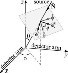
Figure 2: Detector and radiation frames in the FC convention FC .

Using Eqs. (14) and (16), we can write Eq. (15) as

$$Q_{c}^{ij}=-2([\mathbf{e}_{+}^{S}]^{ij}\,\cos 2\Phi_{S}+[\mathbf{e}_{\times}^{S}]^{ij}\,\sin 2\Phi_{S})\,,$$ (19)

where the polarization tensors $\mathbf{e}_{+}^{S}$ and $\mathbf{e}_{\times}^{S}$ are given by

$$\mathbf{e}_{+}^{S}\equiv\mathbf{e}_{1}^{S}\otimes\mathbf{e}_{1}^{S}-\mathbf{e}_{2}^{S}\otimes\mathbf{e}_{2}^{S}\,,\quad\mathbf{e}_{\times}^{S}\equiv\mathbf{e}_{1}^{S}\otimes\mathbf{e}_{2}^{S}+\mathbf{e}_{2}^{S}\otimes\mathbf{e}_{1}^{S}\,.$$ (20)

For a detector lying in the direction $\hat{\mathbf{N}}=\mathbf{e}_{z}^{S}\,\cos\Theta+\mathbf{e}_{x}^{S}\,\sin\Theta$, it is expedient to express GW propagation in the radiation coordinate system with unit vectors {$\mathbf{e}_{x}^{R}$,$\mathbf{e}_{y}^{R}$,$\mathbf{e}_{z}^{R}$} (see our Fig. 1 together with, for instance, Eq. (4.22) of Ref. K ), given by

$$\mathbf{e}^{R}_{x} = \mathbf{e}_{x}^{S}\,\cos\Theta-\mathbf{e}_{z}^{S}\,\sin\Theta\,,$$ (21)

$$\mathbf{e}^{R}_{y} = \mathbf{e}_{y}^{S}\,,$$ (22)

$$\mathbf{e}^{R}_{z} = \mathbf{e}_{x}^{S}\,\sin\Theta+\mathbf{e}_{z}^{S}\,\cos\Theta=\hat{\mathbf{N}}\,.$$ (23)

In writing Eqs. (21)–(23) we used the fact that for a generic binary-detector configuration, the entire system consisting of the binary and the detector can be always rotated along the $z$ axis, in such a way that the detector will lie in the $(x,z)$ plane. Later in this paper (in Sec. IV) we shall find it convenient to conserve the explicit dependence of our formulas on the azimuthal angle $\varphi$ that specifies the direction of the detector.

In the transverse-traceless (TT) gauge, the metric perturbations are

$$\mathbf{h}^{TT}=h_{+}\,{\bf T}_{+}+h_{\times}\,{\bf T}_{\times}\,,$$ (24)

where

$${\bf T}_{+}\equiv\mathbf{e}^{R}_{x}\otimes\mathbf{e}^{R}_{x}-\mathbf{e}^{R}_{y}\otimes\mathbf{e}^{R}_{y}\,,\quad{\bf T}_{\times}\equiv\mathbf{e}^{R}_{x}\otimes\mathbf{e}^{R}_{y}+\mathbf{e}^{R}_{y}\otimes\mathbf{e}^{R}_{x}\,,$$ (25)

and

$$h_{+}=\frac{1}{2}\,h^{ij}\,[\mathbf{T}_{+}]_{ij}\,,\quad h_{\times}=\frac{1}{2}\,h^{ij}\,[\mathbf{T}_{\times}]_{ij}\,.$$ (26)

The response of a ground-based, interferometric detector (such as LIGO or VIRGO) to the GWs is FC

$$h_{\rm resp} = F_{+}\,h_{+}+F_{\times}\,h_{\times}$$ (27)

$$= -\frac{2\mu}{D}\frac{M}{r}\,\left[e_{+}^{S\,ij}\,\cos 2\Phi_{S}+e_{\times}^{S\,ij}\,\sin 2\Phi_{S}\right]([\mathbf{T}_{+}]_{ij}\,F_{+}+[\mathbf{T}_{\times}]_{ij}\,F_{\times})\,,$$

where $F_{+}$ and $F_{\times}$ are the antenna patterns, given by

$$F_{+,\,\times}=\frac{1}{2}[\bar{\mathbf{e}}_{x}\otimes\bar{\mathbf{e}}_{x}-\bar{\mathbf{e}}_{y}\otimes\bar{\mathbf{e}}_{y}]^{ij}[\mathbf{T}_{+,\,\times}]_{ij}\,,$$ (28)

with $\bar{\mathbf{e}}_{x,\,y}$ the unit vectors along the orthogonal interferometer arms. For the geometric configuration shown in Fig. 2, with detector orientation parametrized by the angles $\theta$, $\phi$ and $\psi$, we have

$$F_{+} = \frac{1}{2}(1+\cos^{2}\theta)\,\cos 2\phi\,\cos 2\psi-\cos\theta\,\sin 2\phi\,\sin 2\psi\,,$$ (29)

$$F_{\times} = \frac{1}{2}(1+\cos^{2}\theta)\,\cos 2\phi\,\sin 2\psi+\cos\theta\,\sin 2\phi\,\cos 2\psi\,.$$ (30)

Inserting Eqs. (17), (20), (21)–(23), and (25) into Eq. (27), we get the final result K ,

$$h_{\rm resp}=C_{Q}\,\cos 2\Phi_{S}+S_{Q}\,\sin 2\Phi_{S}\,,$$ (31)

where

$$C_{Q} = -\frac{4\mu}{D}\,(M\,\omega)^{2/3}\,\left[C_{+}\,F_{+}+C_{\times}\,F_{\times}\right]\,,$$ (32)

$$S_{Q} = -\frac{4\mu}{D}\,(M\,\omega)^{2/3}\,\left[S_{+}\,F_{+}+S_{\times}\,F_{\times}\right]\,,$$ (33)

and

$$C_{+} = \frac{1}{2}\cos^{2}\Theta(\sin^{2}\alpha-\cos^{2}i\cos^{2}\alpha)+\frac{1}{2}(\cos^{2}i\sin^{2}\alpha-\cos^{2}\alpha)$$ (34)

$$-\frac{1}{2}\sin^{2}\Theta\sin^{2}i-\frac{1}{4}\sin 2\Theta\sin 2i\cos\alpha\,,$$

$$S_{+} = \frac{1}{2}(1+\cos^{2}\Theta)\cos i\sin 2\alpha+\frac{1}{2}\sin 2\Theta\sin i\sin\alpha\,,$$ (35)

$$C_{\times} = -\frac{1}{2}\cos\Theta(1+\cos^{2}i)\sin 2\alpha-\frac{1}{2}\sin\Theta\sin 2i\sin\alpha\,,$$ (36)

$$S_{\times} = -\cos\Theta\cos i\cos 2\alpha-\sin\Theta\sin i\cos\alpha\,.$$ (37)

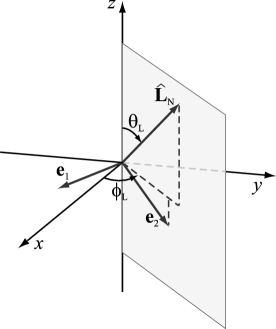
Figure 3: Specification of the initial Newtonian orbital angular momentum in the source frame $\{\mathbf{e}_{x},\mathbf{e}_{y},\mathbf{e}_{z}\}$.

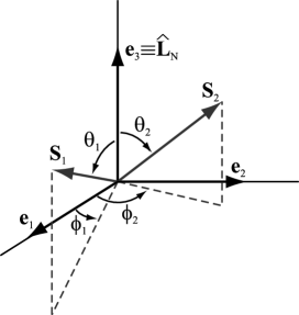
Figure 4: Specification of the initial directions of the spins with respect to the FC orthonormal basis $\{\mathbf{e}_{1},\mathbf{e}_{2},\mathbf{e}_{3}\}$ [Eq. (38)].

II.4 Binary and detector parameters

We shall refer to the total mass $M$, to the mass ratio $\eta=m_{1}\,m_{2}/M^{2}$, and to the magnitudes of the two BH (or NS) spins $S_{1}$ and $S_{2}$ as the basic parameters of the binary. Once these are set, we complete the specification of a binary configuration by giving the initial orbital phase and the components of the orbital and spin angular momenta in the source frame, for a given initial frequency. In our convention, the initial orbital angular momentum is determined by the angles $(\theta_{\rm L_{\rm N}}\equiv i,\phi_{\rm L_{\rm N}}\equiv\alpha)$, as shown in Fig. 3. [In the rest of this paper, we shall use the notation $(\theta_{\rm L_{\rm N}},\phi_{\rm L_{\rm N}})$ to emphasize that these angles define the direction of the orbital angular momentum.] The directions of the spins are specified by the angles $(\theta_{S_{1}},\phi_{S_{1}})$ and $(\theta_{S_{2}},\phi_{S_{2}})$, defined with respect to an orthonormal basis aligned with $\hat{\mathbf{L}}_{\mathrm{N}}$,

$$\mathbf{e}_{1}\equiv\frac{\hat{\mathbf{L}}_{\mathrm{N}}\times\mathbf{e}_{z}^{S}}{|\hat{\mathbf{L}}_{\mathrm{N}}\times\mathbf{e}_{z}^{S}|}\,,\quad\mathbf{e}_{2}\equiv\hat{\mathbf{L}}_{\mathrm{N}}\times\mathbf{e}_{1}\,,\quad\mathbf{e}_{3}\equiv\hat{\mathbf{L}}_{\mathrm{N}}\,,$$ (38)

shown in Fig. 4. We then have

Binary			GW propagation	Detector orientation
$M$, $\eta$, $S_{1}$, $S_{2}$	$\theta_{S_{1}}$, $\theta_{S_{2}}$, $\phi_{S_{1}}-\phi_{S_{2}}$	$\theta_{\rm L_{\rm N}}$, $\phi_{\rm L_{\rm N}}$, $\phi_{S_{1}}+\phi_{S_{2}}$	$\Theta$, $\varphi$	$\theta$, $\phi$, $\psi$
Basic	Local	Directional

Table 1: Classification of binary, GW-propagation, and detector parameters.

$$\hat{\mathbf{S}}_{1} = \mathbf{e}_{1}\,\sin\theta_{S_{1}}\,\cos\phi_{S_{1}}+\mathbf{e}_{2}\,\sin\theta_{S_{1}}\,\sin\phi_{S_{1}}+\mathbf{e}_{3}\,\cos\theta_{S_{1}}\,,$$ (39)

$$\hat{\mathbf{S}}_{2} = \mathbf{e}_{1}\,\sin\theta_{S_{2}}\,\cos\phi_{S_{2}}+\mathbf{e}_{2}\,\sin\theta_{S_{2}}\,\sin\phi_{S_{2}}+\mathbf{e}_{3}\,\cos\theta_{S_{2}}\,.$$ (40)

Among the six angles $(\theta_{\rm L_{\rm N}},\phi_{\rm L_{\rm N}})$, $(\theta_{S_{1}},\phi_{S_{1}})$, and $(\theta_{S_{2}},\phi_{S_{2}})$, only three are intrinsically relevant to the evolution of the binary: $\theta_{S_{1}}$, $\theta_{S_{2}}$ and $\phi_{S_{1}}-\phi_{S_{2}}$. We shall refer to them as local parameters. The other three independent parameters, which are relevant to the computation of the waveform, describe the rigid rotation of the binary as a whole in space, and we shall refer to them as directional parameters. In fact, there are five more directional parameters: $\Theta$ and $\varphi$ specify the direction to the detector in the source frame, and $\theta$, $\phi$, and $\psi$ specify the orientation of the detector with respect to the radiation frame. All these parameters have already been introduced in the previous section. Our classification of the 15 binary and detector parameters is summarized in Tab. 1.

III Analysis of precessional dynamics

In a seminal paper ACST94 , ACST investigated in detail the evolution of binaries of spinning compact objects, focusing on orbital precession and on its influence on the gravitational waveforms. In this section, we build on their analysis to discuss several aspects of quasicircular precessional dynamics that are especially important to the formulation of a reliable DTFs for these systems. Note also that Wex Wex has derived analytic solutions for quasielliptical solutions to the 2PN conservative dynamics, including spin-orbit effects.

We complement ACST’s analytical arguments with the empirical evidence obtained by studying the orbits generated by the numerical integration of Eqs. (1)–(3) and (9). We select the following typical binaries: BBHs with masses $(m_{1}+m_{2})$ given by $(20+10)M_{\odot}$, $(15+15)M_{\odot}$, $(20+5)M_{\odot}$, $(10+10)M_{\odot}$, $(7+5)M_{\odot}$; and NS–BH binaries with masses $m_{1}=10M_{\odot}$ (BH) and $m_{2}=1.4M_{\odot}$ (NS). The BHs are always chosen to be maximally rotating ($S=m^{2}$), while the NSs are assumed to be nonspinning. There are neither astrophysical data nor theoretical results which suggest that maximal spins are preferred. However, in this paper we decide to investigate the most pessimistic (in terms of precessional effects) scenario. The initial GW frequency is chosen at $30\,{\rm Hz}$ for binaries with total mass larger than $20\,M_{\odot}$, and $40\,{\rm Hz}$ for all the other cases. For each set of masses, we consider 1000 (or, when the numerical study is very computationally expensive, only 200) orbital evolutions obtained with random initial orientations of the orbital and spin angular momenta. (These initial configurations are taken from the pseudorandom sequence specified in Sec. VI.2 and used in Sec. VI.3 to evaluate the effectualness DIS1 of our DTF in matching the target signals.)

In Sec. III.1 we introduce the ACST results, and in particular the distinction between simple and transitional precession. In Sec. III.2 we study the dependence of the GW ending frequency (defined in Sec. II.2) on the initial values of spins and on their evolution, and we link this dependence to the conservation of certain functions of the spins through evolution. As mentioned above, a knowledge of the ending frequencies of our target model is important to decide what extension each of the detection templates should have in the frequency domain. In Sec. III.3 we examine the value of the binding energy and of the total angular momentum at the end of evolution, and we estimate the amount of GWs that must be emitted during plunge, merger and ringdown to reduce the spin of the final BH to the maximal value. In Sec. III.4 we discuss, largely on the basis on numerical evidence, the effects of spin on the accumulated orbital phase $\Psi$ [defined by Eq. (10)]; we argue that these effects are mainly nonmodulational, and that, for data-analysis purposes, they can be treated in the same way as the standard PN corrections to the orbits of nonspinning binaries. It follows that the precession of the orbital angular momentum is the primary source of modulations in the signal (as already emphasized by ACST for particular classes of binaries). In Sec. III.5 we show, again on the basis of numerical evidence, that transitional precession has little relevance to the data-analysis problem under consideration. In Sec. III.6 we discuss the power-law approximations introduced by ACST to describe the precession of the orbital plane as a function of frequency in particular binaries, and we show that they are appropriate in general for the larger class of binaries under consideration in this paper. These approximations are a basic building block of the effective template families developed by Apostolatos apostolatos2 and, indeed, of our generalized and improved families.

III.1 The ACST analysis

In their paper ACST94 on precessing binaries of compact objects as GW sources, ACST chose to work at the leading order in both the orbital phasing and the precessional effects to highlight the main features of dynamical evolution. For orbital evolution, they retained only the first term on the right-hand side of Eq. (1): as a consequence, the precession of the orbital plane is the only source of GW modulation considered in the analysis. [The resulting accumulated orbital phase $\Psi$, given by Eq. (10), is known as Newtonian Chirp.] For the precession of the orbital angular momentum and of the spins, ACST retained only the first terms (the spin-orbit terms) in Eqs. (2), (3) and (9). On the basis of these approximations, and in the context of binaries with either $m_{1}\approx m_{2}$ (and spin-spin terms neglected) or $S_{2}\approx 0$, ACST classified the possible evolutions of spinning binaries into two categories: simple precession and transitional precession.

The vast majority of evolutions is characterized by simple precession, where the direction of the total angular momentum remains roughly constant, and where both the orbital angular momentum and the total spin $\mathbf{S}=\mathbf{S}_{1}+\mathbf{S}_{2}$ precess around that direction. ACST provided a simple analytic solution for the evolutions in this class. They also showed that the orbital precession angle, expressed as a function of the orbital frequency, follows approximately a power law (see Eq. (45) of Ref. ACST94 ).

Transitional precession happens when, at some point during the evolution, the orbital angular momentum and the total spin become antialigned and have roughly the same magnitude, so the total angular momentum is almost zero,

$$\mathbf{J}=\mathbf{L}+\mathbf{S}\approx 0\,.$$ (41)

When this condition is satisfied, the total angular momentum is liable to sudden and repeated changes of direction. The evolutions in this class cannot be easily treated analytically, but they occur only for a small portion of the possible initial conditions.

In this paper, we shall refer to the special cases investigated by ACST (with either $m_{1}\approx m_{2}$, or $S_{2}\approx 0$) as ACST configurations. NS–BH binaries and BBHs with $m_{1}\gg m_{2}$ are astrophysically relevant cases among ACST configurations, because for both we can set $S_{2}\approx 0$. The ACST formalism can also describe well BBHs with equal masses, but where spin-spin effects are negligible.

III.2 Conservation laws and GW ending frequencies

For the ACST configurations, both the total spin and its projection on the orbital angular momentum are constants of the motion:

$$\left[\hat{\mathbf{L}}_{\rm N}(t)\cdot\mathbf{S}(t)\right]_{\mbox{\scriptsize ACST}} = \mathrm{const}\,;$$ (42)

$$\left[\mathbf{S}^{2}(t)\right]_{\mbox{\scriptsize ACST}} = \mathrm{const}\,.$$ (43)

For generic non–ACST configurations (as discussed, for instance, by Damour TD ), the effective spin $\mathbf{S}_{\rm eff}$ [Eq. (7)] can, to some extent, replace the total spin in these conservation laws.

From Eqs. (2), (3), and (9), we see also that if we ignore the spin-spin effects in the precession equations, then the projection

$$\kappa_{\rm eff}\equiv\frac{\hat{\mathbf{L}}_{\mathrm{N}}\cdot\mathbf{S}_{\rm eff}}{M^{2}}$$ (44)

of the effective spin onto the Newtonian orbital angular momentum is a constant of motion,

$$\left[\kappa_{\rm eff}(t)\right]_{\rm SO}=\mathrm{const}\,$$ (45)

(where the subscript “SO” stands for the inclusion of spin-orbit effects only); on the other hand, neither $\mathbf{S}^{2}(t)$ nor $\mathbf{S}^{2}_{\rm eff}(t)$ are conserved.

The conservation of $\kappa_{\rm eff}$ has important consequences for the endpoints of evolution, defined in Sec. II.2 by Eq. (13) for the MECO. In the nonspinning case, as discussed in BCV1, if the dynamics was known at all PN orders, then the MECO would agree with the Innermost Stable Spherical Orbit (ISCO), defined as the orbit beyond which circular orbits become dynamically unstable. When only spin-orbit (henceforth, SO) effects are included, the conservation of $\kappa_{\rm eff}$ preserves this correspondence between MECO and ISCO, because the leading-order SO term in the energy is proportional to $\kappa_{\rm eff}$: in fact, the frequency of the MECO has a precise functional dependence on $\kappa_{\rm eff}$ [see Eqs. (11)–(13)].

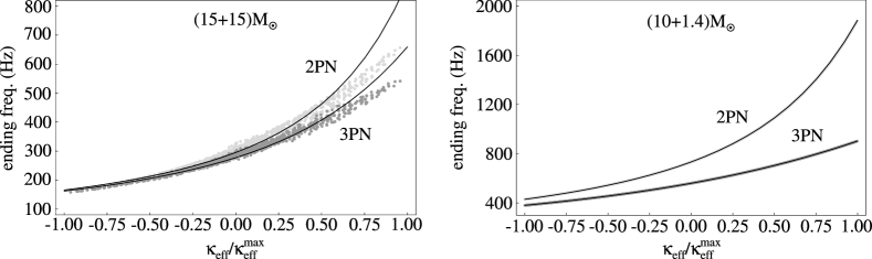
Figure 5: Binary ending frequencies (gray dots) as functions of the initial value of $\kappa_{\rm eff}/\kappa_{\rm eff}^{\rm max}$, for 1000 initial spin configurations of $M=(15+15)M_{\odot}$ BBHs (in the left panel), and $M=(10+1.4)M_{\odot}$ NS–BH binaries (in the right panel), at 2PN and 3.5PN orders. The solid lines plot the SO-only predictions for the ending frequencies.

When spin-spin (henceforth, SS) couplings are also included, $\kappa_{\rm eff}$ is no longer conserved, and the MECOs (and therefore the ending frequencies) of binaries with the same initial $\kappa_{\rm eff}$ become smeared around their SO-only values, which are functions only of $\kappa_{\rm eff}$. In addition to this smearing, the SS contribution to the energy introduces also a bias. In the end, however, the SS correction is not very important for the ending frequencies, as we can see in the following examples. In the left panel of Fig. 5, we plot the ending frequency at 2PN and 3.5PN orders note39 versus the initial value of $\kappa_{\rm eff}$ for BBHs with $M=(15+15)M_{\odot}$ (in gray dots), as compared to the SO-only predictions (in solid lines). The smearing of the ending frequencies is relatively mild, and so is the systematic deviation from the SO-only predictions. We have checked that this behavior characterizes all the mass configurations enumerated just before Sec. III.2, at both 2PN and 3.5PN orders. In the right panel of Fig. 5, we plot the ending frequencies for NS–BH binaries [with $M=(10+1.4)M_{\odot}$]. The ending frequencies follow exactly the expected functional dependence on $\kappa_{\rm eff}$.

The mildness of these deviations can be understood (in part) by looking at the variation of $\kappa_{\rm eff}$ during the evolution. For example, for the $(15+15)M_{\odot}$ BBHs shown in Fig. 5, the maximum deviation of $\kappa_{\rm eff}$ from being a constant (measured as $\mathrm{maxdev}(\kappa_{\rm eff})=[\max(\kappa_{\rm eff})-\min(\kappa_{\rm eff})]/2$) is $0.036$, to be compared with the maximum kinematically allowed deviation, $0.875$; for $(20+5)M_{\odot}$ BBHs at 2PN order, $\mathrm{maxdev}(\kappa_{\rm eff})=0.033$, to be compared with the maximum kinematically allowed deviation $0.92$.

As we can infer from Fig. 5, the ending frequencies depend also on the PN order, and the difference between 2PN and 3.5PN orders is more striking for NS–BH binaries than for BBHs. This trend is present also in the nonspinning case (see BCV1): for nonspinning ($\chi_{1}=\chi_{2}=0$) equal-mass BBHs, we have $\omega_{\rm MECO}^{\rm 2PN}=0.137M^{-1}$ and $\omega_{\rm MECO}^{\rm 3PN}=0.129M^{-1}$. To give a few numbers, for a $(10+10)M_{\odot}$ BBH, we have $f_{\rm GW,2PN}^{\rm MECO}=443\,{\rm Hz}$, and $f_{\rm GW,3PN}^{\rm MECO}=416\,{\rm Hz}$; for a $(15+15)M_{\odot}$ BBH, $f_{\rm GW,2PN}^{\rm MECO}=295\,{\rm Hz}$, and $f_{\rm GW,3PN}^{\rm MECO}=277\,{\rm Hz}$; on the other hand, for a $(10+1.4)\,M_{\odot}$ NS–BH binary, we have $f_{\rm GW,2PN}^{\rm MECO}=734\,{\rm Hz}$, and $f_{\rm GW,3PN}^{\rm MECO}=559\,{\rm Hz}$. For the second and third binaries, these values can be read off from the solid lines of Fig. 5, by setting $\kappa_{\rm eff}=0$ (no spins).

Finally, in Fig. 6 we show the ending frequencies for $(20+5)\,M_{\odot}$ BBHs, when Eq. (1) (which rules the evolution of the orbital phase) is evaluated at 2.5PN order. In this case, if $\kappa_{\rm eff}\geq 0.5$, then $\dot{\omega}$ goes to zero before the MECO can be reached. The resulting ending frequencies deviate considerably from SO-only predictions. As already discussed in BCV1, $\dot{\omega}$ goes to zero because at 2.5PN order the gravitational flux goes to zero for high orbital velocities; since this very nonphysical behavior happens systematically, we then choose to exclude the 2.5PN order from our analysis.

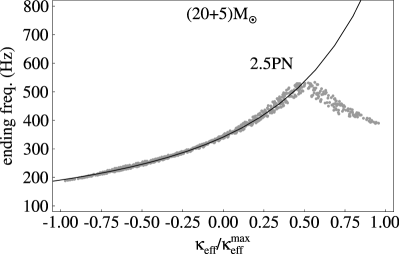
Figure 6: Binary ending frequencies (gray dots) as functions of the initial value of $\kappa_{\rm eff}/\kappa_{\rm eff}^{\rm max}$, for 1000 initial spin configurations of $M=(20+5)M_{\odot}$ BBHs, at 2.5PN order. The solid lines plot the SO-only predictions for the ending frequencies.

III.3 Energy radiated during inspiral and (estimated) total angular-momentum emitted after inspiral

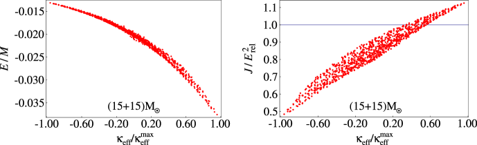
Figure 7: For 1000 $(15+15)M_{\odot}$ BBHs with different initial spin configurations, in the left panel we plot the ratio between the (nonrelativistic) 2PN energy [Eq. (11)] at the ending frequency and the mass-energy initially available $M$, versus the initial $\kappa_{\rm eff}/\kappa_{\rm eff}^{\rm max}$; in the right panel we plot the ratio between the total angular momentum $J$ at 2PN order and the square of the (relativistic) 2PN energy [Eq. (11)] at the ending frequency, versus the initial $\kappa_{\rm eff}/\kappa_{\rm eff}^{\rm max}$.

It is interesting to evaluate how much energy can be radiated in GWs before the final plunge, especially for binaries whose inspiral end in the LIGO–VIRGO frequency band. In the left panel of Fig. 7, for $M=(15+15)M_{\odot}$ BBHs, we plot the ratio between the 2PN (nonrelativistic) energy, given by Eq. (11) and evaluated at the endpoint of evolution (as defined in Sec. II.2), and the total mass–energy initially available, $M$. Depending on the initial relative orientation between the spins and the orbital angular momentum (as expressed by the initial $\kappa_{\rm eff}/\kappa_{\rm eff}^{\rm max}$), the energy that can be released in GWs during the inspiral ranges between $\sim 1.5$ and $3.5\%$ of $M$. More energy can be emitted when the initial spins are aligned with the orbital angular momentum. We find similar results for all the other BBHs investigated, and similar results were also obtained by Damour in the EOB framework (see Fig. 1 of Ref. TD ).

It is also interesting to estimate how much total angular momentum can be radiated during the coalescence phases that follow the inspiral (plunge and merger), especially when those phases fall in the LIGO–VIRGO band. In general, we have

$$\mathbf{J}_{\rm rad}=\mathbf{J}-\mathbf{S}_{\rm BH}\,,$$ (46)

where $\mathbf{J}_{\rm rad}$ is the angular momentum radiated during plunge–merger, $\mathbf{J}$ is the total angular momentum of the binary at the end of the inspiral, and $\mathbf{S}_{\rm BH}$ is the spin of the final black hole. A lower limit on the angular momentum radiated in these phases can be obtained using the fact that the magnitude of the final spin can be at most $M^{2}_{\rm BH}$ (where $M_{\rm BH}$ is the mass of the final black hole). To derive this lower limit we follow Flanagan and Hughes FH , and we write, using Eq. (46),

$$|\mathbf{J}_{\rm rad}|\geq|\mathbf{J}|-|\mathbf{S}_{\rm BH}|\geq|\mathbf{J}|-M_{\rm BH}^{2}\geq|\mathbf{J}|-E_{\rm rel}^{2}\,,$$ (47)

where $E_{\rm rel}=M+E$ is the relativistic energy of the binary at the end of inspiral; in deriving Eq. (47) we used the relation $|\mathbf{S}_{\rm BH}|\leq M_{\rm BH}^{2}\leq E_{\rm rel}^{2}$. It is straightforward to see from Eq. (47) that this lower limit is nontrivial (that is, greater than zero) only when $|\mathbf{J}|>E_{\rm rel}^{2}$.

In the right panel of Fig. 7, for $M=(15+15)M_{\odot}$ BBHs, we plot $|\mathbf{J}|/E_{\rm rel}^{2}$, where the angular momentum is evaluated at 2PN order [KWW, ,K, ],

$$\mathbf{J}/M^{2} = \eta\,(M\omega)^{-1/3}\,\hat{\mathbf{L}}_{N}\,\left\{1+\frac{(9+\eta)}{6}\,(M\omega)^{2/3}-\frac{7}{3}\,\hat{\mathbf{L}}_{N}\cdot\frac{\mathbf{S}_{\rm eff}}{M^{2}}\,(M\omega)+\left[\frac{1}{24}(81-57\eta+\eta^{2})\right.\right.$$ (48)

$$\left.\left.-\frac{1}{\eta}\,\left(\frac{\mathbf{S}_{1}}{M^{2}}\cdot\frac{\mathbf{S}_{2}}{M^{2}}-3\left(\hat{\mathbf{L}}_{N}\cdot\frac{\mathbf{S}_{1}}{M^{2}}\right)\left(\hat{\mathbf{L}}_{N}\cdot\frac{\mathbf{S}_{2}}{M^{2}}\right)\right)\right]\,(M\omega)^{4/3}\right\}-\eta\,(M\omega)^{2/3}\,\frac{\mathbf{S}_{\rm eff}}{M^{2}}+\frac{\mathbf{S}}{M^{2}}\,.$$

We see that $J/E_{\rm rel}^{2}$ is generally less than one, except when $\kappa_{\rm eff}\geq 0.4$ (which happens for $13\%$ of all the initial spin configurations); the maximum value of $|\mathbf{J}|/E_{\rm rel}^{2}$ is $1.13$. (For a similar plot obtained in the EOB framework see Fig. 2 of Ref. TD .) Such large values of $\kappa_{\rm eff}$ imply large ending frequencies [for the $(15+15)M_{\odot}$ BBHs shown, larger than 400 Hz], which do not lie in the LIGO–VIRGO band of good interferometer sensitivity, unless the BBHs have higher masses; then all the frequencies are scaled down. In any case, for $\kappa_{\rm eff}=1$ (spins and orbital momenta initially aligned), in the high-mass binaries investigated, Eq. (47) suggests the lower limit

$$|\mathbf{J}_{\rm rad}|\geq 0.13\,E_{\rm rel}^{2}\sim 0.1\,M^{2},$$ (49)

to be compared with the value $0.4M^{2}$ obtained by Flanagan and Hughes FH using BH spins aligned with the orbital angular momentum (estimated to be $\sim 0.9M^{2}$).

A (trivial) upper limit for $\mathbf{J}_{\rm rad}$ is obtained by setting $\mathbf{S}_{\rm BH}=0$:

$$|\mathbf{J}^{\rm rad}|\leq|\mathbf{J}|\,.$$ (50)

For different values of $\kappa_{\rm eff}$, the upper limit for our $(15+15)M_{\odot}$ binary is $\sim 0.5$ – $1.1M^{2}$. However, in order for the inspiral to end within the LIGO–VIRGO band of good interferometer sensitivity (which requires a MECO frequency lower than 400 Hz), we need $\kappa_{\rm eff}<0.4$, which corresponds to an upper limits $\sim 0.5$ – $0.7\,M^{2}$.

To put this section into context, we point out that most reliable PN estimates for the energy and the angular momentum radiated after the MECO can be achieved only with models that include information about the plunge phase, such as the model that can be built on Damour’s spinning-EOB equations TD .

III.4 Spin-orbit and spin-spin effects on the accumulated orbital phase

	Maximum modulational correction $\Delta\Psi^{\mathrm{res}}$
	$(20+10)M_{\odot}$	$(15+15)M_{\odot}$	$(20+5)M_{\odot}$	$(10+10)M_{\odot}$	$(7+5)M_{\odot}$	$(10+1.4)M_{\odot}$ [NS–BH]
$\langle\Delta\Psi^{\rm res}\rangle_{200}$	0.0247	0.0214	0.0450	0.0402	0.0828	0.1228
$\Delta\Psi^{\rm res}_{90\%\,(200)}$	0.0460	0.0411	0.0676	0.0787	0.1504	0.1884
$\max_{200}\Delta\Psi^{\rm res}$	0.0680	0.0523	0.1227	0.1186	0.2196	0.1895

Table 2: Maximum modulational effects in the accumulated orbital phase $\Psi$. We give the average over the 200 samples, the 90% quantile of the distribution, and the maximum value for the diagnostic $\Delta\Psi^{\rm res}$, defined in Eq. (53).

While for nonspinning binaries the accumulated orbital phase [defined by Eq. (10)] coincides with (half) the GW phase at the detector, for spinning binaries the two phases differ by precessional effects; in the FC convention, these are found in part in the relation

$$\dot{\Phi}_{S}=\dot{\Psi}-\dot{\alpha}\cos i,$$ (51)

where $\Phi_{S}$ is the orbital phase with respect to the ascending node of the orbit, which appears in Eq. (31) for the detector response to GW; and in part in the explicit time dependence of the coefficients $C_{Q}$ and $S_{Q}$ on $\alpha$ and $i$ [see Eqs. (32)–(37)]. In this section, we are going to argue that the evolution of the accumulated orbital phase is very similar in spinning and nonspinning binaries; and that, as a consequence, the effect of spins on detector response through the accumulated orbital phase can be reproduced using nonspinning-binary templates, such as those studied in BCV1 [see also Eqs. (92)–(94)]. Of course, precessional effects do enter the detector response through the other dependences mentioned above, and these cannot be neglected when building templates to detect physical signals.

Both the spin-orbit and spin-spin couplings can affect the accumulated orbital phase $\Psi$ through the 1.5PN and 2PN terms in Eq. (1). However, as we shall discuss in this section, this effect is largely nonmodulational. For each binary configuration, we introduce three different functions of time: (a) the accumulated orbital phase $\Psi^{\rm full}$, obtained by solving the full set of Eqs. (1)–(3) and (9), including the SO and SS couplings; (b) the accumulated orbital phase $\Psi^{\rm fix}$, obtained by using the initial orbital angular momentum and spins at all times in the SO and SS couplings; and (c) the accumulated orbital phase $\Psi^{\rm nospin}$ for a nonspinning binary, obtained by dropping the SO and SS couplings altogether.

In general, $\Psi^{\rm fix}$ and $\Psi^{\rm nospin}$ are quite different for the same set of binary masses. However, the difference $\Psi^{\rm fix}-\Psi^{\rm nospin}$ is not a strongly oscillating function (that is, it does not show any modulation), and it can be reduced considerably by modifying the 1.5PN and 2PN coefficients in the phasing equation for the nonspinning binary. It is then reasonable to assume that such a nonmodulational effect could be captured by the nonspinning DTFs constructed in BCV1. Moreover, the difference between $\Psi^{\rm full}$ and $\Psi^{\rm fix}$ is due to the nonconservation of the SO and SS terms that appear in Eq. (1) for $\dot{\omega}$. These terms have relatively high PN orders, so we expect that they will be small.

Thus, we expect that $\Psi^{\rm full}$ can be well described by a nonmodulational phasing of the kind

$$\Psi^{\rm nonmod}(f)={\cal C}_{0}+{\cal C}_{1}\,f+\frac{{\cal C}_{2}}{f^{5/3}}+\frac{{\cal C}_{3}}{f^{2/3}}\,,$$ (52)

which looks rather like the frequency-domain phasings employed in the DTFs of BCV1. [Here $\mathcal{C}_{2}$ and $\mathcal{C}_{3}$ can be seen as actual (intrinsic) template parameters, whereas $\mathcal{C}_{0}$ and $\mathcal{C}_{1}$ represent, respectively, the initial phase and the time of arrival of the GW signal, both of which are extrinsic parameters in the sense discussed in BCV1.] To verify this hypothesis, we first evaluate $\Psi^{\rm full}$ in the frequency range $50\,{\rm Hz}\mbox{--}250\,{\rm Hz}$ (which is appropriate for first-generation ground-based GW detectors), using Eqs. (1)–(3) and (9) at 2PN order, for all the BBH and NS–BH configurations considered earlier [(5 + 1) masses $\times$ 200 angles]. We then (least-square) fit $\Psi^{\rm full}$ with functions of the form (52). A measure of the goodness of the fit, given by

$$\Delta\Psi^{\rm res}=\max_{50\,{\rm Hz}<f<250\,{\rm Hz}}\left|\Psi^{\rm full}(f)-\Psi^{\rm nonmod}(f)\right|\,,$$ (53)

is shown in Tab. III.4. The maximum deviations are all smaller than $\sim 0.1\,{\rm rad}$, except for the lighter $(7+5)M_{\odot}$ BBH and $(10+1.4)M_{\odot}$ NS–BH systems (where however the average deviations are still $\sim 0.1\,{\rm rad}$). This suggests that templates with phasing expressions similar to (52) (such as those proposed in BCV1) could already approximate rather well the full target model studied in this paper.

III.5 Simple and transitional precession of total angular momentum

	Percentage of binary configurations where $\exists t:\hat{\mathbf{J}}(t)\cdot\hat{\mathbf{J}}(0)<1-\epsilon_{J}$
	$(20+10)M_{\odot}$	$(15+15)M_{\odot}$	$(20+5)M_{\odot}$	$(10+10)M_{\odot}$	$(7+5)M_{\odot}$	$(10+1.4)M_{\odot}$ [NS–BH]
$\epsilon_{\rm J}=0.05$	$17.5\%$	$6.0\%$	$33.5\%$	$7.0\%$	$3.5\%$	$0.0\%$
$\epsilon_{\rm J}=0.10$	$2.5\%$	$0.0\%$	$11.0\%$	$0.0\%$	$0.0\%$	$0.0\%$

Table 3: Deviation of the total angular momentum $\hat{\mathbf{J}}$ from its initial direction. This table shows the percentage of the binary configurations where $\hat{\mathbf{J}}(t)\cdot\hat{\mathbf{J}}(0)$ goes below $1-\epsilon_{\rm J}$, for the $\epsilon_{\rm J}$ given in the first column.

For most of the binary configurations investigated, we find, in analogy with the ACST analysis, that the direction of total angular momentum does not change much during evolution. In other words, transitional precession does not occur. Table 3 shows the fraction of configurations that yield

$$\min_{t}\hat{\mathbf{J}}(t)\cdot\hat{\mathbf{J}}_{0}<1-\epsilon_{\rm J}\,,$$ (54)

when $\epsilon_{\rm J}=0.05$ and $0.10$. Let us now try to understand the numbers of Tab. 3 in more detail.

We first focus on the columns two to six, which deal with binaries of maximally spinning BHs. For BBHs with single masses $m=5\mbox{--}20\,M_{\odot}$, the total spin is not usually large enough to satisfy the transitional-precession condition (41), as we can prove easily by using all the evolution equations at the leading PN order: during the evolution, the magnitude of the orbital angular momentum decreases with the GW frequency $f$, as in

$$|\mathbf{L}|\approx|\mathbf{L}_{\rm N}|=\eta\,(\pi Mf)^{-1/3}M^{2}\,,$$ (55)

while the total spin is bounded by

$$|\mathbf{S}|<|\mathbf{S}_{1}|+|\mathbf{S}_{2}|=m_{1}^{2}+m_{2}^{2}=(1-2\eta)M^{2}\,.$$ (56)

In order for transitional precession to occur, we need at the very least $|\mathbf{L}_{\rm N}|=|\mathbf{S}|$ [see Eq. (41)], which requires

$$\eta(\pi Mf)^{-1/3}<(1-2\eta)\,,$$ (57)

or

$$f>f_{\rm trans}^{\rm min}\equiv\frac{\eta^{3}}{\pi M(1-2\eta)^{3}}\,.$$ (58)

For transitional precession to occur before we reach the Schwarzschild ISCO frequency $f_{\rm Schw}=1/\sqrt{6^{3}}\pi M$, we then need

$$\frac{f_{\rm trans}^{\rm min}}{f_{\rm Schw}}=\left(\frac{\sqrt{6}\eta}{1-2\eta}\right)^{3}\gtrsim 1\quad\Rightarrow\quad\eta\gtrsim 0.22\,.$$ (59)

Although the ending frequencies obtained within our target model are usually higher than $f_{\rm Schw}$, the very configurations that can have transitional precession (those with nearly antialigned total spin and orbital angular momenta) have always lower ending frequencies, making 0.22 too large an estimate for the critical value of $\eta$.

Figure 8: Transitional precession. Evolution of the direction of total angular momentum (left panel) and of Newtonian orbital angular momentum (right panel) in the transitionally precessing $(20+5)M_{\odot}$ BBH with initial angles $\theta_{S_{1}}=175.4^{\circ}$, $\theta_{S_{2}}=105.4^{\circ}$, and $\phi_{S_{1}}-\phi_{S_{2}}=92.0^{\circ}$ (at $f_{\rm GW}=30\,{\rm Hz}$).

As a consequence, among all the configurations we have considered, only $(20+5)M_{\odot}$ and $(20+10)M_{\odot}$ BBHs can then have observable transitional-precession phases. These latter binaries are characterized by significantly larger changes in $\mathbf{J}$ [see Tab. 3]. However, $(20+10)M_{\odot}$ BBHs still require $f>f_{\rm tran}^{\rm min}=138\,{\rm Hz}$, which is very close to the relevant ending frequency; so the change in $\mathbf{J}$ is smaller, and we never observed episodes of transitional precession in the 200 initial configurations analyzed. On the contrary, we observed a few for $(20+5)M_{\odot}$ BBHs; one example follows from the initial configuration given by $\theta_{S_{1}}=175.4^{\circ}$, $\theta_{S_{2}}=105.4^{\circ}$, and $\phi_{S_{1}}-\phi_{S_{2}}=92.0^{\circ}$ (at $f_{\rm GW}=30\,{\rm Hz}$). In this configuration the initial spin of the more massive body is almost exactly antialigned with the orbital angular momentum. The trajectories of $\hat{\mathbf{J}}$ and $\hat{\mathbf{L}}_{\mathrm{N}}$ during this evolution are shown, respectively, in the left and right panels of Fig. 8.

By contrast, none of the NS–BH configurations examined exhibits transitional precessions. This is because the BH is taken as maximally spinning, so $\mathbf{S}$ is always much larger than $\mathbf{L}$ in the frequency band under consideration.

III.6 Apostolatos’ power law for orbital precession

Figure 9: Simple precession. The upper graphs show the evolution of the direction of total angular momentum $\hat{\mathbf{J}}$ (left), and of Newtonian orbital angular momentum $\hat{\mathbf{L}}_{\mathrm{N}}$ (right), in the case of the simply precessing $(20+5)M_{\odot}$ BBH with initial angles $\theta_{S_{1}}=44.6^{\circ}$, $\theta_{S_{2}}=101.0^{\circ}$, and $\phi_{S_{1}}-\phi_{S_{2}}=-39.7^{\circ}$ (at $30\,{\rm Hz}$). The lower graphs show the projection of $\hat{\mathbf{L}}_{\mathrm{N}}$ onto the plane perpendicular to the initial $\hat{\mathbf{J}}$ (left), and the angle between $\hat{\mathbf{L}}_{\mathrm{N}}$ and $\hat{\mathbf{J}}$, plotted as a function of inverse GW frequency (right). The BBH was rotated in space so that the initial direction of $\hat{\mathbf{J}}$ would be parallel to the $z$ axis.

As discussed in the previous section, the vast majority of binary configurations undergoes simple precession, where $\hat{\mathbf{J}}$ remains constant, while $\hat{\mathbf{L}}_{\mathrm{N}}$ and $\mathbf{S}_{1,2}$ precess around it. For ACST configurations ($m_{1}\approx m_{2}$ and negligible SS interactions, or $S_{2}\approx 0$), both $\hat{\mathbf{L}}_{N}$ and $\hat{\mathbf{S}}$ precess around $\mathbf{J}$ with the precession frequency (ACST94, , Eq. (42))

$$\Omega_{\rm p}\equiv\frac{d\alpha_{\rm p}}{dt}=\left(2+\frac{3}{2}\,\frac{m_{2}}{m_{1}}\right)J\omega^{2}\,.$$ (60)

ACST identified two regimes where the evolution of $\alpha_{\rm p}$ can be approximated very well by a power law in $\omega$ (or $f$). For $L_{N}\gg S$, the total angular-momentum $J\approx L_{N}\sim\omega^{-1/3}$; using $\dot{\omega}\sim\omega^{11/3}$, it is straightforward to derive from Eq. (60) that $\alpha_{\rm p}$ is approximated well by a linear function of $f^{-1}$,

$$\alpha_{\mathrm{p}(-1)}^{\mathrm{fit}}(f)\approx\frac{{\cal B}_{1}}{f}+{{\cal B}_{2}}\,,$$ (61)

where ${\cal B}_{1}$ and ${\cal B}_{2}$ are constant coefficients. Since $L_{N}/S\sim\eta\,\omega^{-1/3}$, the condition $L_{N}\gg S$ corresponds to comparable-mass binaries ($\eta\sim 1/4$) or to large separations. For $L_{N}\ll S$, we have $J\approx S$; in this case we derive from Eq. (60) that $\alpha_{\rm p}$ is approximated well by a linear function of $f^{-2/3}$,

$$\alpha^{\mathrm{fit}}_{\mathrm{p}(-2/3)}(f)\approx\frac{{\cal B}^{\prime}_{1}}{f^{2/3}}+{{\cal B}^{\prime}_{2}}\,,$$ (62)

where ${\cal B}^{\prime}_{1}$ and ${\cal B}^{\prime}_{2}$ are constant coefficients. The condition $L_{N}\ll S$ corresponds to $m_{1}\ll m_{2}$ or to small separations (late inspiral).

It turns out that Eqs. (61) and (62) apply also to a large fraction of the BBHs and NS–BH binaries studied in this paper. This can be tested semiquantitatively by the following procedure. For each configuration, we take the precession angle $\alpha_{\rm p}(f)$ and we fit it with a function $\alpha_{\mathrm{p}(-1,-2/3)}^{\mathrm{fit}}(f)$ of the form (61) or (62), for frequencies in the range $50$–$250\,{\rm Hz}$. We then evaluate the maximum difference

$$\Delta\alpha_{\mathrm{max}(-1,-2/3)}\equiv\max_{50\,{\rm Hz}<f<250\,{\rm Hz}}\left|\alpha_{\rm p}(f)-\alpha_{\mathrm{p}(-1,-2/3)}^{\rm fit}(f)\right|\,.$$ (63)

In Tab. 4, we show the values of $\Delta\alpha_{\mathrm{max}(-1)}^{90\%}$ (that is, the 90% percentile of $\Delta\alpha_{\mathrm{max}(-1)}$) and $\Delta\alpha_{\mathrm{max}(-2/3)}^{90\%}$, for $(15+15)M_{\odot}$, $(20+10)M_{\odot}$, $(10+10)M_{\odot}$, and $(7+5)M_{\odot}$ BBHs, and for $(10+1.4)M_{\odot}$ NS–BH binaries. The numbers show that Eqs. (61) and (62) yield (roughly) comparable approximation. This result is confirmed also by the more detailed analyses discussed later in this paper.

Figure 9 plots the 2PN evolutions of $\hat{\mathbf{J}}$ (upper left panel) and $\hat{\mathbf{L}}_{\mathrm{N}}$ (upper right panel) for a $(20+5)M_{\odot}$ BBH with initial conditions $\theta_{S_{1}}=44.6^{\circ}$, $\theta_{S_{2}}=101.0^{\circ}$, and $\phi_{S_{1}}-\phi_{S_{2}}=-39.7^{\circ}$ (at $30\,{\rm Hz}$). The figure plots also the projection of $\hat{\mathbf{L}}_{\mathrm{N}}$ onto the plane perpendicular to the initial $\hat{\mathbf{J}}$ (lower left panel), and the precession angle $\alpha_{\rm p}$ between $\hat{\mathbf{L}}_{\mathrm{N}}$ and $\hat{\mathbf{J}}$, plotted as a function of inverse GW frequency $f^{-1}$ (lower right panel), and showing a very nearly linear dependence.

	90% percentiles of error in precession angle, $\Delta\alpha_{\mathrm{max}}$
	$(15+15)M_{\odot}$	$(20+10)M_{\odot}$	$(20+5)M_{\odot}$	$(10+10)M_{\odot}$	$(7+5)M_{\odot}$	$(10+1.4)M_{\odot}$ [NS–BH]
$\Delta\alpha_{\mathrm{max}(-1)}^{90\%}$	$0.30$	$0.24$	$0.23$	$0.34$	$0.64$	$0.61$
$\Delta\alpha_{\mathrm{max}(-2/3)}^{90\%}$	$0.52$	$0.48$	$0.50$	$0.68$	$1.14$	$0.72$

Table 4: Approximation of binary precession histories using best-fit parameters $\mathcal{B}_{1}$ and $\mathcal{B}_{2}$ in Eqs. (61) and (62). This table shows the 90% percentiles of $\Delta\alpha_{\mathrm{max}(-1)}$ [Eq. (63)] and $\Delta\alpha_{\mathrm{max}(-2/3)}$ in the BBH and NS–BH populations studied throughout this section.

Building on the results obtained by ACST, Apostolatos apostolatos2 conjectured (quite reasonably) that orbital precession will modulate the gravitational waveforms with functional dependencies given by Eqs. (61) and (62). On the basis of this conjecture and of the observation that, in matched-filtering techniques, matching the phase of signals is more important than matching their amplitudes, Apostolatos proposed a family of detection templates apostolatos2 obtained by modifying the phasing of nonspinning PN templates as in

$$\mbox{Apostolatos' ansatz:}\quad\psi_{\rm spinning}\rightarrow\psi_{\rm non\,spinning}+{\cal C}\cos(\delta+{\cal B}f^{-2/3})\,,$$ (64)

while keeping a Newtonian amplitude $f^{-7/6}$. Recently, Grandclément, Kalogera and Vecchio GKV applied Apostolatos’ suggestion to an approximated analytical model of NS–BH binaries and low-mass BBHs: whereas the addition of phase modulations according to Eq. (64) did increase the effectualness DIS1 of nonspinning PN templates, the resulting DTF family was still not good enough to recommend its application when trying to capture the real modulated waveforms. Moreover, this DTF requires three additional intrinsic parameters (${\cal C},\delta$, and ${\cal B}$) on top of the two BH (or NS) masses. The resulting GW searches would then be plagued by an extremely high computational cost.

In the rest of this paper, we shall propose a better template family, inspired by old and new insight on the precessional effects that appear in the gravitational waveforms. As we shall see, Apostolatos’ ansatz can be improved to build DTFs that have both high effectualness DIS1 and low computational requirements.

IV Definition of modulated DTFs for precessing binaries

We are now going to bring together all the observations reported in Sec. III to build DTFs that perform well in capturing the detector response to the GWs emitted by precessing binaries of NSs and spinning BHs (at least as long as the actual physical signals are modeled faithfully enough by the adiabatic target model described in Sec. II).

In Sec. IV.1 we develop a new (as far as we know) convention for the generation and propagation of GW from spinning binaries; this convention has the desirable property of factorizing the waveform into a carrier signal whose phase is essentially the accumulated orbital phase of the binary, and a modulated amplitude term which is sensitive to the precession of the orbital plane. In Sec. IV.2 we then use the results of Sec. III.4 to build an approximation of the carrier signal, and the results of Secs. III.2, III.5, and III.6 to build an approximation to the modulated amplitude; using these terms together, we define three families of detection templates. In Sec. IV.3 we describe two standard families of nonspinning-binary templates; in Sec. VI we shall compare their performance with the performance of our DTFs, to evaluate the performance improvements brought about by our treatment of precession.

IV.1 A new convention for GW generation in spinning binaries

At least two conventions are used to express the gravitational waveforms generated by binaries of spinning compact objects, as computed in the quadrupolar approximation note40 : the ACST convention ACST94 , which uses a rotating reference frame, and the FC convention FC , which uses a nonrotating reference frame. We discussed the FC convention in Sec. II.3, and we used it throughout this paper to generate gravitational waveforms from the numerical integration of the equations of motion of the target model. Before going to the specific conventions, we shall first sketch a generic procedure to write the gravitational waveform.

In general, the unit vector along the separation vector of the binary, $\hat{\mathbf{n}}(t)$, and the unit vector along the corresponding relative velocity, $\hat{\mathbf{\lambda}}(t)$, can be written as

$$\hat{\mathbf{n}}(t)=\mathbf{e}_{1}(t)\,\cos\Phi(t)+\mathbf{e}_{2}(t)\,\sin\Phi(t)\,,\quad\hat{\mathbf{\lambda}}(t)=-\mathbf{e}_{1}(t)\,\sin\Phi(t)+\mathbf{e}_{2}(t)\,\cos\Phi(t)\,,$$ (65)

where $\mathbf{e}_{1}(t)$, $\mathbf{e}_{2}(t)$, and $\mathbf{e}_{3}(t)\equiv\hat{\mathbf{L}}_{N}(t)$ are orthonormal vectors, and $\mathbf{e}_{1,2}(t)$ forms a basis for the instantaneous orbital plane [see Fig. 4]; the quantity $\Phi(t)$ is then the orbital phase with respect to $\mathbf{e}_{1,2}(t)$. The definition of $\mathbf{e}_{1,2}(t)$ and of $\Phi(t)$ is not unique: an arbitrary function of time can be added to $\Phi(t)$, and then compensated by a time-dependent rotation of $\mathbf{e}_{1,2}(t)$ around $\hat{\mathbf{L}}_{N}(t)$, leaving $\hat{\mathbf{n}}(t)$ and $\hat{\mathbf{\lambda}}(t)$ unchanged. In nonspinning binaries the orbital plane (and therefore $\hat{\mathbf{L}}_{N}$) does not precess, so the natural choice is to keep $\mathbf{e}_{1,2}$ constant. In spinning binaries $\hat{\mathbf{L}}_{N}(t)$ precesses, and different, but nonetheless meaningful, conventions can be given for $\mathbf{e}_{1,2}(t)$ and $\Phi(t)$. Note that $\Phi(t)$ is not, in general, the same as the accumulated orbital phase $\Psi(t)=\int\omega(t)\,dt$. Given a convention for $\mathbf{e}_{1,2}(t)$ and $\Phi(t)$, the tensor $Q_{c}^{ij}$ that appears in Eq. (14) can be written as

$$Q^{ij}_{c}=-2\left([\mathbf{e}_{+}]^{ij}\cos 2\Phi+[\mathbf{e}_{\times}]^{ij}\sin 2\Phi\right)$$ (66)

where

$$\mathbf{e}_{+}=\mathbf{e}_{1}\otimes\mathbf{e}_{1}-\mathbf{e}_{2}\otimes\mathbf{e}_{2}\,,\quad\mathbf{e}_{\times}=\mathbf{e}_{1}\otimes\mathbf{e}_{2}+\mathbf{e}_{2}\otimes\mathbf{e}_{1}\,.$$ (67)

With the detector lying along the direction $\hat{\mathbf{N}}$, one goes on to define a radiation frame, formed by orthonormal vectors $\mathbf{e}_{x}^{R}$, $\mathbf{e}_{y}^{R}$ and $\mathbf{e}_{z}^{R}=\hat{\mathbf{N}}$. The GW response is then given by

$$h_{\rm resp}=-\frac{2\mu}{D}\frac{M}{r}\,\underbrace{\left([\mathbf{e}_{+}]^{ij}\,\cos 2\Phi+[\mathbf{e}_{\times}]^{ij}\,\sin 2\Phi\right)}_{\mathrm{factor\;Q:\;quadrupole\;moment}}\underbrace{\left([\mathbf{T}_{+}]_{ij}\,F_{+}+[\mathbf{T}_{\times}]_{ij}\,F_{\times}\right)}_{\mathrm{factor\;P:\;detector\;projection}}\,,$$ (68)

where the tensors $[\mathbf{T}_{+,\times}]_{ij}$ are given by (25), namely

$${\bf T}_{+}\equiv\mathbf{e}^{R}_{x}\otimes\mathbf{e}^{R}_{x}-\mathbf{e}^{R}_{y}\otimes\mathbf{e}^{R}_{y}\,,\quad{\bf T}_{\times}\equiv\mathbf{e}^{R}_{x}\otimes\mathbf{e}^{R}_{y}+\mathbf{e}^{R}_{y}\otimes\mathbf{e}^{R}_{x}\,,$$ (69)

and where $F_{+}$ and $F_{\times}$ are given by Eq. (28), namely

$$F_{+,\,\times}=\frac{1}{2}[\bar{\mathbf{e}}_{x}\otimes\bar{\mathbf{e}}_{x}-\bar{\mathbf{e}}_{y}\otimes\bar{\mathbf{e}}_{y}]^{ij}[\mathbf{T}_{+,\,\times}]_{ij}\,,$$ (70)

with $\bar{\mathbf{e}}_{x,\,y}$ the unit vectors along the orthogonal arms of the interferometer. Again, $\mathbf{e}_{x}^{R}$ and $\mathbf{e}_{y}^{R}$ are not uniquely defined, because they can be rotated at will around $\hat{\mathbf{N}}$, of course changing the values of $F_{+}$ and $F_{\times}$.

ACST refer $\Phi(t)$ to the direction $\hat{\mathbf{N}}$ of GW propagation, by imposing that $\mathbf{e}^{\rm ACST}_{1}(t)\propto\hat{\mathbf{N}}\times\hat{\mathbf{L}}_{N}(t)$; they also set $\mathbf{e}_{x}^{R}(t)\propto\pm\hat{\mathbf{N}}\times\hat{\mathbf{L}}_{\mathrm{N}}(t)$. Although the ACST convention has allowed some insight into the waveforms, it is rather inconvenient for the purpose of data analysis, because almost all the quantities that come into Eq. (68) [$\mathbf{e}_{1,\,2}$, $\mathbf{T}_{+,\,\times}$, and $F_{+,\,\times}$] depend both on the time evolution of the binary and on the direction to the detector. Using the terminology introduced in Sec. II.3 and Tab. 1, under the ACST convention the local and directional parameters are entangled in a time-dependent manner.

FC introduce the fixed source axes $\{\mathbf{e}^{S}_{x},\mathbf{e}^{S}_{y},\mathbf{e}^{S}_{z}\}$ [see Sec. II.3], and they impose that $\mathbf{e}^{S}_{1}(t)\propto\mathbf{e}^{S}_{z}\times\hat{\mathbf{L}}_{N}(t)$ [see Eq. (17)]. The radiation frame does not change with time [see Eqs. (21)–(23)]. As a consequence, the factors Q and P in Eq. (68) become disentangled: factor Q expresses the components of the quadrupole moment, which depend only on the evolution of the binary inside the source frame; factor P expresses the projection of the quadrupole moment onto the radiation frame and onto the antisymmetric mode of the detector, which depend only on the relative orientation between the source frame and the detector. However, for our purposes there are still two shortcomings in the FC convention:

1. The FC convention defines $\mathbf{e}_{1,2}(t)$ and $\Phi(t)$ in terms of the fixed source frame $\mathbf{e}^{S}_{x,y,z}$, which is quite artificial, because only the relative orientation between binary and detector affects the detector response $h_{\rm resp}$.

2. In Sec. III.4 we saw that the accumulated orbital phase $\Psi(t)$ is (almost) nonmodulated, so the modulations of the waveform come mainly from the precession of the orbital plane. Under the FC convention, the modulations appear only in factor Q of Eq. (68), but they appear both in the phase $\Phi(t)$ and in the precession of the tensors $\mathbf{e}_{+,\times}(t)$. It would be nice to isolate the precessional effects in either element.

Both issues would be solved if we could find a modification of the FC convention where $\Phi$ coincides with the accumulated orbital phase, $\Psi$. As it turns out, it is possible to do so: we need to redefine the vectors $\mathbf{e}_{1,2}(t)$ so that they precess alongside $\hat{\mathbf{L}}_{N}$,

$$\dot{\mathbf{e}}_{i}(t)=\mathbf{\Omega}_{e}(t)\times\mathbf{e}_{i}(t)\,,\quad i=1,2\,,$$ (71)

with

$$\mathbf{\Omega}_{e}(t)\equiv\mathbf{\Omega}_{L}(t)-[\mathbf{\Omega}_{L}(t)\cdot\hat{\mathbf{L}}_{N}(t)]\,\hat{\mathbf{L}}_{N}(t)\,,$$ (72)

where $\mathbf{\Omega}_{L}$ is obtained by collecting the terms that (cross-product) multiply $\hat{\mathbf{L}}_{N}$ in Eq. (9). In App. B we prove that this convention yields $\dot{\Phi}=\omega=\dot{\Psi}$, as desired. Qualitatively, one can reason as follows. The angular velocity of the binary lies along $\hat{\mathbf{L}}_{N}(t)$, and has magnitude $\dot{\Psi}=\omega$. The reason why $\Phi$ and $\Psi$ differ is that the orbital basis $\mathbf{e}_{1,2}$, used to define $\Phi$, must rotate to keep up with the precession of the orbital plane. However, the difference vanishes if we constrain the angular velocity of $\mathbf{e}_{1,2}$ to be orthogonal to $\hat{\mathbf{L}}_{N}$; Eq. (72) provides just the right constraint. In the following, we shall refer to our new convention as the precessing convention.

convention	factor P	factor Q
	$\mathbf{T}_{+,\times}\quad\quad\quad F_{+,\times}$	$\Phi(t)$	$\mathbf{e}_{+,\times}(t)$
ACST
FC
precessing

Table 5: Parametric dependence of the building elements of the detector response function $h_{\mathrm{resp}}$ [Eq. (68)] under the ACST, FC, and precessing conventions.

In Tab. 5 we summarize the parameter dependence of the terms that make up the detector response function [Eq. (68)], under the three conventions. It is important to remark that in the precessing convention the polarization tensors $\mathbf{e}_{+,\,\times}(t)$, as geometric objects, do not depend on the source frame, but only on the basic and local parameters. In practice, however, we need to introduce an arbitrary choice of the source frame to relate the orientation of the binary to the direction and orientation of the detector (that is, to write explicitly the products $[\mathbf{e}_{+,\,\times}]_{ij}[\mathbf{T}_{+,\,\times}]_{ij}$). We can avoid this arbitrariness by setting the source frame according to the initial configuration of the binary at a fiducial orbital frequency; for example, we can impose (without loss of generality)

$$\mathbf{e}_{x}^{S}\propto\mathbf{S}_{1}(0)-[\mathbf{S}_{1}(0)\cdot\hat{\mathbf{L}}_{\mathrm{N}}(0)]\hat{\mathbf{L}}_{\mathrm{N}}(0)\,,\quad\mathbf{e}_{y}^{S}=\hat{\mathbf{L}}_{\mathrm{N}}(0)\times\mathbf{e}_{x}^{S}\,,\quad\mathbf{e}_{z}^{S}=\hat{\mathbf{L}}_{\mathrm{N}}(0)\,,$$ (73)

and

$$\mathbf{e}_{1}(0)=\mathbf{e}_{x}^{S}\,,\quad\mathbf{e}_{2}(0)=\mathbf{e}_{y}^{S}\,,\quad\mathbf{e}_{3}(0)=\mathbf{e}_{z}^{S}\,.$$ (74)

[If $\mathbf{S}_{1}(0)$ and $\hat{\mathbf{L}}_{\mathrm{N}}(0)$ are parallel, $\mathbf{e}_{x}^{S}$ can be chosen to lie in any direction within the plane orthogonal to $\hat{\mathbf{L}}_{\mathrm{N}}(0)$.] Then the initial conditions, as expressed by their components with respect to the source frame, are determined only by the local parameters,

$$\hat{\mathbf{L}}_{\mathrm{N}}(0) = (0,0,1)\,,$$ (75)

$$\mathbf{S}_{1}(0) = (\sin\theta_{S_{1}},0,\cos\theta_{S_{1}})\,,$$ (76)

$$\mathbf{S}_{2}(0) = (\sin\theta_{S_{2}}\cos(\phi_{S_{2}}-\phi_{S_{1}}),\sin\theta_{S_{2}}\sin(\phi_{S_{2}}-\phi_{S_{1}}),\cos\theta_{S_{2}})\,,$$ (77)

along with an initial orbital phase $\Psi_{0}$ given by

$$\mathbf{n}(0)=\mathbf{e}_{1}(0)\cos\Psi_{0}+\mathbf{e}_{2}(0)\sin\Psi_{0}\,.$$ (78)

With this choice, all the directional parameters are isolated in factor P of Eq. (68), while the basic and local parameters (which affect the dynamics of the binary) are isolated in factor Q. We will call upon this property of the precessing convention in Sec. VI.4, where we propose a new family of templates for NS–BH binaries built by writing a set of orthonormal component templates that contain all the dynamical information expressed by factor Q, and then using their linear combinations to reproduce the projection operation expressed by factor P.

Going back to the main thrust of this section, we obtain the detector response $h_{\mathrm{resp}}$ by setting the direction to the detector $\hat{\mathbf{N}}$ (specified by the angles $\Theta$ and $\varphi$ with respect to the source frame), and by introducing the radiation frame, oriented along the axes

$$\mathbf{e}_{x}^{R} = -\mathbf{e}_{x}^{S}\,\sin\varphi+\mathbf{e}_{y}^{S}\,\cos\varphi\,,$$ (79)

$$\mathbf{e}_{y}^{R} = -\mathbf{e}_{x}^{S}\,\cos\Theta\cos\varphi-\mathbf{e}_{y}^{S}\,\cos\Theta\,\sin\varphi+\mathbf{e}_{z}^{S}\,\sin\Theta\,,$$ (80)

$$\mathbf{e}_{z}^{R} = +\mathbf{e}_{x}^{S}\,\sin\Theta\,\cos\varphi+\mathbf{e}_{y}^{S}\,\sin\Theta\,\sin\varphi+\mathbf{e}_{z}^{S}\,\cos\Theta=\hat{\mathbf{N}}\,;$$ (81)

we then get

$$h_{\rm resp}=-\frac{2\mu}{D}\frac{M}{r}\,\left([\mathbf{e}_{+}]^{ij}\,\cos 2\Psi+[\mathbf{e}_{\times}]^{ij}\,\sin 2\Psi\right)\left([\mathbf{T}_{+}]_{ij}\,F_{+}+[\mathbf{T}_{\times}]_{ij}\,F_{\times}\right)\,.$$ (82)

Applying the stationary-phase approximation (SPA) at the leading order, we can write the Fourier transform of $h_{\rm resp}$ as

$$\tilde{h}_{\rm resp}(f)=-\tilde{h}_{C}(f)\,\left([\mathbf{e}_{+}(t_{f})]^{jk}+i\,[\mathbf{e}_{\times}(t_{f})]^{jk}\right)\,\left([\mathbf{T}_{+}]_{jk}\,F_{+}+[\mathbf{T}_{\times}]_{jk}\,F_{\times}\right)\quad\mathrm{for\;}f>0\,,$$ (83)

where $\tilde{h}_{C}(f)$ is the SPA Fourier transform of the carrier signal,

$$h_{C}=\frac{2\mu}{D}\,\frac{M}{r}\,\cos 2\Psi\,,$$ (84)

and where $t_{f}$ is the time at which the carrier signal has instantaneous frequency $f$.

IV.2 Definition of a new DTF for precessing binaries

By adopting the precessing convention, we isolate all the modulational effects due to precession in the evolving polarization tensors $[\mathbf{e}_{+,\times}]^{ij}$ (these effects will show up both in the amplitude and in the phase of $h_{\mathrm{resp}}$). The discussion of Sec. III.4 shows that, to a very good approximation, the carrier signal is not modulated, so we expect that $\tilde{h}_{C}(f)$ should be approximated well by the nonspinning PN templates studied in BCV1, or variations thereof. As for the time dependence of the tensors $[\mathbf{e}_{+,\times}]^{ij}$, the discussion of Secs. III.5 and III.6 suggests that we adopt the Apostolatos’ ansatz ApostolatosFF , and write expressions in the generic forms

$$[\mathrm{e}_{+,\times}]^{ij}[\mathbf{T}_{+,\times}]_{jk}\propto\mathcal{C}_{+,\times}\cos\left(\mathcal{B}\,f^{-2/3}+\delta_{+,\times}\right)\quad\mbox{or}\quad\propto\mathcal{C}_{+,\times}\cos\left(\mathcal{B}\,f^{-1}+\delta_{+,\times}\right)\,.$$ (85)

Indeed, our extended numerical investigations provide evidence that expressions of the form (85) should work quite well for the binaries under consideration.

All these elements suggest that we introduce a family of detection templates of the general (Fourier-domain) form

$$h(\psi_{\mathrm{NM}},\mathcal{A}_{k},t_{0},\alpha_{k};f)=\left[\sum^{n}_{k=1}(\alpha_{k}+i\alpha_{k+n})\mathcal{A}_{k}(f)\right]e^{2\pi ift_{0}}e^{i\psi_{\mathrm{NM}}(f)}\quad(\mathrm{for}\;f>0)$$ (86)

[and $h(f)=h^{*}(-f)$ for $f<0$], where the $\mathcal{A}_{k}(f)$ are real amplitude functions, the $\alpha_{k}$ are their (real) coefficients, and $t_{0}$ is the time of arrival of the GW signals. The function $\psi_{\mathrm{NM}}$ represents the phase of the unmodulated carrier signal; we write it as a series in the powers of $f^{1/3}$,

$$\psi_{\mathrm{NM}}(f)=f^{-5/3}\,(\psi_{0}+\psi_{1/2}f^{1/3}+\psi_{1}f^{2/3}+\psi_{3/2}f+\ldots)\,.$$ (87)

As discussed in BCV1, this phasing works well for relatively high-mass, nonspinning BBHs, and for NS–BH binaries; in addition, as anticipated in Sec. III.4, the PN coefficients $\psi_{i}$ are able to capture the nonmodulational effects of spin-orbit and spin-spin couplings on the orbital phase. In this paper we examine three specific families of detection templates of this form, listed in Tab. 6. The subscripts “2”, “4”, and “6” in our abbreviations for the template families denote the number of $\alpha_{k}$ coefficients that appear in Eq. (86).

The families $(\psi_{0}\psi_{3/2})_{2}$ and $(\psi_{0}\psi_{3/2}\alpha)_{4}$ were already studied in Ref. BCV1 for the case of nonspinning binaries. Both families contain the leading $f^{-7/6}$ Newtonian dependence of the amplitude; however, $(\psi_{0}\psi_{3/2}\alpha)_{4}$ contains a correction to the Newtonian amplitude (introduced in BCV1, where it was parametrized by $\alpha$) which can account for the variation of the rate of inspiral in the late stages of orbital evolution. The first family is given by

$$(\psi_{0}\psi_{3/2})_{2}:\quad h(\ldots;f)=(\alpha_{1}+i\alpha_{2})f^{-7/6}\,\theta(f_{\mathrm{cut}}-f)\,e^{2\pi ift_{0}}\exp i[\psi_{0}f^{-5/3}+\psi_{3/2}f^{-2/3}];$$ (88)

here $\alpha_{1}+i\alpha_{2}$ can also be written as $\mathcal{A}\exp i\phi^{\mathrm{GW}}_{0}$, where $\phi^{\mathrm{GW}}_{0}$ is the initial GW phase, and $\mathcal{A}$ is an overall normalization factor for the template. So the two $\alpha_{k}$ coefficients encode the initial global phase of the waveform, plus a normalization factor. The second family is given by

$$(\psi_{0}\psi_{3/2}\alpha)_{4}:\quad h(\ldots;f)=[(\alpha_{1}+i\alpha_{2})f^{-7/6}+(\alpha_{3}+i\alpha_{4})f^{-1/2}]\,\theta(f_{\mathrm{cut}}-f)\,e^{2\pi ift_{0}}\exp i[\psi_{0}f^{-5/3}+\psi_{3/2}f^{-2/3}];$$ (89)

another way to rewrite the coefficients $\alpha_{1\mbox{--}4}$ more physically is $\mathcal{A}\exp[i\phi^{\mathrm{GW}}_{0}]f^{-7/6}(1+\alpha\exp[i\phi^{\alpha}]f^{2/3})$, where $\alpha$ is the additional amplitude parameter and $\phi^{\alpha}$ is the relative phase of the amplitude correction (as in BCV1, in this paper we always set $\phi^{\alpha}=0$). So the four coefficients $\alpha_{k}$ encode the global phase, the strength of the correction to the Newtonian amplitude, and the relative phase of this correction with respect to the Newtonian amplitude, plus an overall normalization factor.

The third family, $(\psi_{0}\psi_{3/2}\mathcal{B})_{6}$, contains the leading Newtonian amplitude, modified by two modulation terms [a generalization of the Apostolatos’ ansatz (85)] that account for the precession of the orbital angular momentum due to spin effects. It is given by

$$(\psi_{0}\psi_{3/2}\mathcal{B})_{6}:\quad h(\ldots;f) = f^{-7/6}[(\alpha_{1}+i\alpha_{2})+(\alpha_{3}+i\alpha_{4})\cos(\mathcal{B}f^{-2/3})+(\alpha_{5}+i\alpha_{6})\sin(\mathcal{B}f^{-2/3})]$$ (90)

$$\quad\quad\quad\times\,\theta(f_{\mathrm{cut}}-f)\,e^{2\pi ift_{0}}\exp i[\psi_{0}f^{-5/3}+\psi_{3/2}f^{-2/3}];$$

another way to rewrite the six coefficients $\alpha_{1\mbox{--}6}$ in close analogy to Apostolatos’ ansatz is

$$\mathcal{A}\,e^{i\phi^{\mathrm{GW}}_{0}}f^{-7/6}\left[1+\mathcal{C}\,e^{i\phi^{\mathrm{mod}}}\cos(\beta f^{-2/3}+\delta_{1}+i\delta_{2})\right]$$

$$\equiv \mathcal{A}\,e^{i\phi^{\mathrm{GW}}_{0}}f^{-7/6}\left[1+\mathcal{C}_{\mathrm{cos}}\,e^{i\phi^{\mathrm{cos}}}\cos(\beta f^{-2/3})+\mathcal{C}_{\mathrm{sin}}\,e^{i\phi^{\mathrm{sin}}}\sin(\beta f^{-2/3})\right]$$

(where all the coefficients are still real). So the six coefficients $\alpha_{k}$ encode the global phase, the strength of the amplitude modulation, its relative phase with respect to the Newtonian amplitude, and the internal (complex) phase of the modulation. It is clear that our family implements a generalization of Apostolatos’ ansatz, because we allow a complex phase offset between the Newtonian and the sinusoidal amplitude terms, and also between the cosine and sine modulational terms. We consider also a variant $(\psi_{0}\psi_{3/2}\mathcal{B}^{\prime})_{6}$ of this family where the $f^{-2/3}$ frequency dependence in the sinusoidal amplitude functions is replaced by $f^{-1}$.

Template family	$\psi_{\mathrm{NM}}(f)$	$\mathcal{A}_{1}$(f)	$\mathcal{A}_{2}(f)$	$\mathcal{A}_{3}(f)$
$(\psi_{0}\psi_{3/2})_{2}$	$\psi_{0}f^{-5/3}+\psi_{3/2}f^{-2/3}$	$f^{-7/6}\,\theta(f_{\mathrm{cut}}-f)$
$(\psi_{0}\psi_{3/2}\alpha)_{4}$	$\psi_{0}f^{-5/3}+\psi_{3/2}f^{-2/3}$	$f^{-7/6}\,\theta(f_{\mathrm{cut}}-f)$	$f^{-1/2}\,\theta(f_{\mathrm{cut}}-f)$
$(\psi_{0}\psi_{3/2}\mathcal{B})_{6}$	$\psi_{0}f^{-5/3}+\psi_{3/2}f^{-2/3}$	$f^{-7/6}\,\theta(f_{\mathrm{cut}}-f)$	$f^{-7/6}\cos(\mathcal{B}f^{-2/3})\,\theta(f_{\mathrm{cut}}-f)$	$f^{-7/6}\sin(\mathcal{B}f^{-2/3})\,\theta(f_{\mathrm{cut}}-f)$
$(\psi_{0}\psi_{3/2}\mathcal{B}^{\prime})_{6}$	$\psi_{0}f^{-5/3}+\psi_{3/2}f^{-2/3}$	$f^{-7/6}\,\theta(f_{\mathrm{cut}}-f)$	$f^{-7/6}\cos(\mathcal{B}f^{-1})\,\theta(f_{\mathrm{cut}}-f)$	$f^{-7/6}\sin(\mathcal{B}f^{-1})\,\theta(f_{\mathrm{cut}}-f)$

Table 6: Specification of the DTFs examined in this paper.

For all three families, the templates are terminated at a cut frequency $f_{\mathrm{cut}}$, above which the amplitude drops to zero; this $f_{\mathrm{cut}}$ is in effect one of the (intrinsic) search parameters. For all three families, the frequency dependence of the phase includes the leading Newtonian term, $f^{-5/3}$, and a term $f^{-2/3}$ that corresponds to the 1.5PN correction in the phase evolution of nonspinning binaries (as obtained, in the SPA, by integrating the energy-balance equation through an adiabatic sequence of circular orbits, using PN expanded energy and flux). In BCV1 we found that including either the 1PN or 1.5PN term is in general sufficient to model the phase evolution of nonspinning binaries of high mass.

IV.3 Definition of the standard SPA template families

In this section we define two families of standard nonspinning-binary templates, obtained by solving the Taylor-expanded energy-balance equation for an adiabatic sequence of quasicircular orbits, and using the stationary-phase approximation (SPA) to express the result as a function of the GW frequency $f$ (see BCV1). In Sec. VI we compare the matching performance of these templates to the performance of our new DTFs, to show that the various tricks used to build the new families do indeed improve their effectualness DIS1 . The standard SPA families are built from the analytic expressions of Refs. 2PN ; 2.5PNand3.5PN . The frequency-domain phasing (under the assumption of nonevolving orbital angular momentum and spins) is given by apostolatos2

$$\psi_{\rm SPA}(f)=2\pi\,f\,t_{c}-\phi_{c}+\frac{3}{128}\,(\pi{\cal M}\,f)^{-5/3} \!\!\!\!\left[1+\frac{20}{9}\,\left(\frac{743}{336}+\frac{11}{4}\eta\right)\,(\pi M\,f)^{2/3}\,-4(4\pi-{\rm SO})\,(\pi M\,f)\right.$$ (92)

$$\;\;\left.+10\,\left(\frac{3058673}{1016064}+\frac{5429}{1008}\eta+\frac{617}{144}\eta^{2}-{\rm SS}\right)\,(\pi M\,f)^{4/3}\right]\,,$$

where ${\cal M}=M\eta^{3/5}$ is the chirp mass, and where ${\rm SO}$ and ${\rm SS}$ are the spin-orbit and spin-spin terms, given explicitly by

$${\rm SO} = \frac{1}{M^{2}}\,\left[\left(\frac{113}{12}+\frac{25}{4}\,\frac{m_{2}}{m_{1}}\right)\,\mathbf{S}_{1}+\left(\frac{113}{12}+\frac{25}{4}\,\frac{m_{1}}{m_{2}}\right)\,\mathbf{S}_{2}\right]\cdot\hat{\mathbf{L}}_{N}\,,$$ (93)

$${\rm SS} = \frac{1}{48m_{1}\,m_{2}\,M^{2}}\,\left[-247\,\mathbf{S}_{1}\cdot\mathbf{S}_{2}+721(\mathbf{S}_{1}\cdot\hat{\mathbf{L}}_{N})\,(\mathbf{S}_{2}\cdot\hat{\mathbf{L}}_{N})\right]\,.$$ (94)

We neglect all PN corrections to the amplitude, by adopting its Newtonian functional form, $f^{-7/6}$; we also neglect all precessional effects, by setting $\mathrm{SO}=\mathrm{SS}=0$. Templates of this form are routinely used in searches for GW signals from nonspinning binaries. In that case, the templates are generally ended at the GW frequency corresponding to the Schwarzschild ISCO $f_{\rm Schw}\simeq 0.022/M$. We denote such templates as SPAs. We introduce also a variant of this family, SPAc, characterized by the additional frequency-cut parameter $f_{\mathrm{cut}}$, used also in our DTFs. Altogether, we get

$$\mathrm{SPAs}:h(\mathcal{M},\eta,t_{0},\psi_{0},\alpha_{N};f)=\alpha_{N}f^{-7/6}\theta(f_{\mathrm{Schw}}-f)e^{2\pi ift_{0}}\exp i[\psi_{\mathrm{SPA}}+\psi_{0}];$$ (95)

$$\mathrm{SPAc}:h(\mathcal{M},\eta,f_{\mathrm{cut}},t_{0},\psi_{0},\alpha_{N};f)=\alpha_{N}f^{-7/6}\theta(f_{\mathrm{cut}}-f)e^{2\pi ift_{0}}\exp i[\psi_{\mathrm{SPA}}+\psi_{0}].$$ (96)

V GW data analysis with the DTF

In searching for GW signals using matched-filtering techniques, we construct a discrete bank of templates that represent all the possible signals that we expect to receive from a given class of sources. We then proceed to compare each stretch of detector output with each of the templates, computing their overlap (essentially, a weighted correlation). A high value of the overlap statistic for a given stretch of detector output and for a particular template implies that there is a high probability that during that time the detector actually received a GW signal similar to the template. This technique is intrinsically probabilistic because, for any template, detector noise alone can (rarely) yield high values of the statistic. In general, the higher the value of the statistic, the harder it is to obtain it from noise alone. So it is important to set the detection threshold (above which we confidently claim a detection) by considering the resulting probability of the false alarms caused by noise.

To verify whether the DTFs developed in Sec. V can be used to search reliably and effectually for the GWs from spinning binaries, we need to evaluate the fitting factor FF of the DTFs in matching the target signals for a variety of binary and detector parameters. The FF is defined as the ratio between the overlap of the target signal with the best possible template in the family and the overlap of the target signal with itself note41 . So in Sec. V.1 we discuss the maximization of the overlap over template parameters for a given target signal. The other important element to evaluate the reliability and effectualness DIS1 of the DTFs are the detection thresholds that the DTFs yield for a given false-alarm probability. In Sec. V.2 we discuss these thresholds under the simplifying hypothesis of Gaussian detector noise. The material presented in this section builds on the treatment of matched-filtering data analysis for GW sources given in Sec. II of BCV1 (which is built on Refs. DA ; DIS1 ; DIS3 ), and it uses the same notations.

V.1 Maximization of the overlap over template parameters

Among all the template parameters that appear in Eq. (86), we are going to treat the $\psi_{i}$, $f_{\mathrm{cut}}$ and $\mathcal{B}$ as intrinsic parameters; and the $\alpha_{k}$ and $t_{0}$ as extrinsic parameters: that is, when we look within one of our DTFs for the template that best matches a given target signal, we will need to consider explicitly many different values of the $\psi_{i}$, of $f_{\mathrm{cut}}$, and of $\mathcal{B}$; however, for any choice of these parameters, the best $\alpha_{k}$ and $t_{0}$ are determined automatically by simple algebraic expressions (see Sec. II B of BCV1). For the next few paragraphs, where we discuss the optimization of the coefficients $\alpha_{k}$, we shall not indicate the dependence of the templates on the intrinsic parameters.

For a given signal $s$, we seek the maximum of the overlap,

$$\max_{t_{0},\alpha_{k}}\,\langle s,h(t_{0},\alpha_{k})\rangle\,,$$ (97)

under the normalization condition

$$\langle h(t_{0},\alpha_{k}),h(t_{0},\alpha_{k})\rangle=1$$ (98)

[this condition is necessary to set a scale for the statistic distribution of the overlap between a given template and pure noise]. Here the inner product $\langle g,h\rangle$ of two real signals with Fourier transforms $\tilde{g}$, $\tilde{h}$ is defined by

$$\langle g,h\rangle=2\int_{-\infty}^{+\infty}\frac{\tilde{g}^{*}(f)\tilde{h}(f)}{S_{n}(|f|)}df=4\,\mathrm{Re}\int_{0}^{+\infty}\frac{\tilde{g}^{*}(f)\tilde{h}(f)}{S_{n}(f)}df$$ (99)

(see BCV1). We proceed constructively: first, we build a new set of amplitude functions $\hat{\mathcal{A}}_{k}(f)$ that are linear combinations of the $\mathcal{A}_{k}(f)$, and that satisfy the orthonormality condition $\langle\hat{\mathcal{A}}_{i}(f),\hat{\mathcal{A}}_{j}(f)\rangle=\delta_{ij}$ for $i,j=1,2,\ldots n$; we then define an orthonormal set of single-$\hat{\mathcal{A}}_{k}$ templates,

$$\hat{h}_{k}(t_{0};f)\equiv\hat{\mathcal{A}}_{k}(f)e^{2\pi ift_{0}}e^{i\psi_{\mathrm{NM}}}\,,\quad\quad\hat{h}_{k+n}(t_{0};f)\equiv i\hat{\mathcal{A}}_{k}(f)e^{2\pi ift_{0}}e^{i\psi_{\mathrm{NM}}}\quad(\mathrm{for}\;f>0)$$ (100)

[and $\hat{h}_{k}(f)=\hat{h}_{k}^{*}(-f)$ for $f<0$], which satisfy $\langle\hat{h}_{i}(t_{0}),\hat{h}_{j}(t_{0})\rangle=\delta_{ij}$ (with $i,j=1,2,\ldots,2n$) for any $t_{0}$. The maximized overlap [Eq. (97)] can now be rewritten as

$$\max_{t_{0},\alpha_{k}}\,\langle s,h(t_{0},\alpha_{k})\rangle=\max_{t_{0}}\max_{\hat{\alpha}_{k}}\sum_{k=1}^{2n}\hat{\alpha}_{k}\langle s,\hat{h}_{k}(t_{0})\rangle\,,$$ (101)

while the condition (98) is now simply $\sum_{k=1}^{2n}\hat{\alpha}_{k}^{2}=1$. The inner maximum of Eq. (101) (over the $\hat{\alpha}_{k}$) is achieved when

$$\hat{\alpha}_{k}=\frac{\langle s,\hat{h}_{k}(t_{0})\rangle}{\sqrt{\sum_{j=1}^{2n}\langle s,\hat{h}_{j}(t_{0})\rangle^{2}}}\,,$$ (102)

and the maximum overlap itself is

$$\max_{t_{0},\alpha_{k}}\,\langle s,h(t_{0},\alpha_{k})\rangle=\max_{t_{0}}\max_{\hat{\alpha}_{k}}\sum_{k=1}^{2n}\hat{\alpha}_{k}\langle s,\hat{h}_{k}(t_{0})\rangle=\sqrt{\max_{t_{0}}\sum_{j=1}^{2n}\langle s,\hat{h}_{j}(t_{0})\rangle^{2}}\,.$$ (103)

This happens essentially because the sum in Eq. (101) can be seen as a scalar product in a $2n$-dimensional Euclidean space, which is maximized when the unit $2n$-vector $\hat{\alpha}_{k}$ lies along the direction of the $2n$-vector $\langle s,\hat{h}_{k}(t)\rangle$. The quantities $\langle s,\hat{h}_{j}(t_{0})\rangle$ for $j=1,2,3,\ldots,n$ are given by the two related Fourier integrals

$$\langle s,\hat{h}_{j}\rangle = 2\,\mathrm{Re}\,\int^{+\infty}_{0}\frac{\hat{\mathcal{A}}_{j}(f)e^{i\psi_{\mathrm{NM}}(f)}s^{*}(f)}{S_{h}(f)}\,e^{2\pi ift_{0}}df\,,$$ (104)

$$\langle s,\hat{h}_{j+n}\rangle = -2\,\mathrm{Im}\,\int^{+\infty}_{0}\frac{\hat{\mathcal{A}}_{j}(f)e^{i\psi_{\mathrm{NM}}(f)}s^{*}(f)}{S_{h}(f)}\,e^{2\pi ift_{0}}df\,.$$ (105)

We now go back to discussing the full set of template parameters. The relevant measure of the effectualness DIS1 of a template family at matching a physical signal $s$ is the fitting factor FF,

$$\mathrm{FF}=\max_{t_{0},\alpha_{k},f_{\mathrm{cut}},\psi_{i}}\,\frac{\langle s,h(t_{0},\alpha_{k})\rangle}{\sqrt{\langle s,s\rangle}}\,,$$ (106)

(see, for instance, Sec. II of BCV1) which is maximized over the $\alpha_{k}$, but also over the time of arrival $t_{0}$ (also an extrinsic parameter), and over all the intrinsic parameters, $\psi_{i}$, $f_{\mathrm{cut}}$, and $\mathcal{B}$. The fitting factor is a function of the physical parameters of the physical signal $s$, and of course of the template family used to match it. We define also the signal amplitude SA for a given signal,

$$\mathrm{SA}=\sqrt{\langle s,s\rangle}.$$ (107)

SA gives the optimal overlap obtained for a template that is exactly equal to the signal (except for its normalization), and it is inversely proportional to the luminosity distance to the source; where we do not indicate otherwise, we always assume the fiducial distance $d_{0}=100$ Mpc.

The maximization of the overlap over $t_{0}$ is easy to obtain, because the integrals (104) and (105) can be evaluated at the same time for all the $t_{0}$ using Fast Fourier Transform techniques Schutz . On the other hand, the maximization over $f_{\mathrm{cut}}$ and over the other intrinsic parameters is obtained by an explicit search over a multidimensional parameter range, where we look for the maximum of the partially maximized (over extrinsic parameters) overlap, given by Eq. (97). For all the actual searches discussed in this paper we employ with good results the simplicial algorithm amoeba nrc .

V.2 False-alarm statistics of the DTFs

In the practice of GW data analysis, template families are used to build discrete template banks parametrized by a discrete set of ntuples of the intrinsic parameters. Then each of the templates is correlated with the detector output, to see if the detection statistic [in our case, the partially maximized correlation (97)] is greater than the detection threshold. It is important to notice that the statistic is already maximized with respect to the extrinsic parameters, while the intrinsic parameters serve as labels for each of the templates. Therefore, we are effectively setting up a separate detection test for each of the templates in the bank.

In this section we are going to evaluate the false-alarm probability for one such test, defined as the probability that detector noise alone will yield an overlap greater than the detection threshold. The total false-alarm probability is then obtained by multiplying the false-alarm probability for a single template by the number $\mathcal{N}_{\mathrm{shapes}}$ of independent signal shapes (generally of the same order of magnitude as the number of templates in the bank), and by the number $\mathcal{N}_{\mathrm{times}}$ of possible times of arrival $t_{0}$, distanced in such a way that the displaced templates are essentially orthogonal note42 . At the end of this exercise, we are going to set the detection threshold so that the total false-alarm probability is acceptably low.

Under the assumption of Gaussian noise, the inner product $\langle n,\hat{h}_{j}\rangle$ of noise $n$ alone with a normalized template component $\hat{h}_{i}$ is (by construction) a Gaussian random variable with zero mean and unit variance (see, for instance, Sec. II of BCV1). Because (for the same $t_{0}$ and for the same intrinsic parameters) all the $\hat{h}_{j}$ are orthogonal, the inner products $\langle n,\hat{h}_{j}\rangle$ (for $j=1,\ldots,2n$) are all independent normal variables. It follows that the statistic $X=\max_{t_{0},\alpha_{k}}\,\langle n,h(t_{0},\alpha_{k})\rangle$ [see Eq. (103)], given by the square root of the sum of their squares, follows the $\chi$ distribution with $2n$ degrees of freedom, characterized by the probability density function and cumulative distribution function

$$\mathrm{PDF}_{\chi(2n)}(X=x)=\frac{x^{2n-1}e^{-x^{2}/2}}{2^{n-1}\Gamma(n)},\quad\mathrm{CDF}_{\chi(2n)}(X<x)=\frac{\Gamma(n,0,x^{2}/2)}{\Gamma(n)},$$ (108)

where we have used the generalized incomplete gamma function $\Gamma(n,z_{0},z_{1})=\int_{z_{0}}^{z_{1}}t^{n-1}e^{-t}dt$. For $n=1$ we obtain the Rayleigh distribution, typical of the maximization of the amplitude of signals with two quadratures.

In Tab. 7 we show the thresholds needed to obtain a total false alarm probability of $10^{-3}$, with $\mathcal{N}_{\mathrm{times}}=3\,10^{10}$ (typical of about three years of observation with LIGO), and with the $\mathcal{N}_{\mathrm{shapes}}$ given in the first column. We observe that each time we increase $\mathcal{N}_{\mathrm{shapes}}$ by one order of magnitude, the threshold increases by about 2% (this happens uniformly for all $n$’s). On the other hand, each step in $n$ increases the threshold by about 4%. Thus, when we design DTFs we should keep in mind that the best possible overlap increases with the number of templates employed, and with the complexity of the templates (clearly, the complexity of our DTFs increases with the number of amplitude functions); but the detection threshold increases as well, reducing the number of signals that pass the detection test. So in principle we are justified in using more numerous and more complex templates only if the gain in the overlap is larger than the increase in the detection threshold.

The prospects shown in Tab. 7 for the models with $n=2$ and $n=3$ improve somewhat if we constrain the values that the $\alpha_{k}$ can attain when they are (algebraically) maximized. We can do this, for instance, if we judge that certain combinations of the $\alpha_{k}$ correspond to unphysical waveforms, but then we must be consistent and exclude any detections that cross the threshold within the excluded parameter region. In any case, we should remember that our study of false-alarm statistics is based on the idealization of Gaussian noise, which will not be realized in practice: real-world data-analysis schemes relie on matched-filtering techniques complemented by vetoing schemes 40meter , which remove detection candidates using nonlinear tests on the signal. Therefore, any DTF should be evaluated in that context before it is excluded for producing excessive detection thresholds within the Gaussian analysis.

$\mathcal{N}_{\mathrm{shapes}}$	Threshold for false-alarm probability $=10^{-3}$
	$(\psi_{0}\,\psi_{3/2})_{2}$	$(\psi_{0}\,\psi_{3/2}\,\alpha)_{4}$	$(\psi_{0}\,\psi_{3/2}\,\mathcal{B})_{6}$
	$n=1$	$n=2$	$n=3$
$10^{2}$	8.44	8.87	9.22
$10^{3}$	8.71	9.13	9.48
$10^{4}$	8.97	9.39	9.73
$10^{5}$	9.22	9.63	9.97
$10^{6}$	9.47	9.87	10.21

Table 7: Detection thresholds for a false-alarm probability $=10^{-3}$ for a $\chi$-distributed detection statistic with $2n$ degrees of freedom, for $\mathcal{N}_{\mathrm{times}}=3\,10^{10}$, and for the $\mathcal{N}_{\mathrm{shapes}}$ given in the first column. The values given for $(\psi_{0},\psi_{3/2}\,\alpha)_{4}$ do not take into account the $\phi^{\alpha}=0$ constraint.

VI Evaluation of DTF performance

We wish to investigate the effectualness DIS1 of our DTFs in matching the GW signals generated by precessing binaries of spinning compact objects, at least as approximated by the target model described in Sec. II. To do so, we shall evaluate the fitting factor FF [Eq. (106)] of the DTFs over a population of binaries with a variety of basic, local and directional parameters, and compare the results with the FF obtained for the standard SPA families [Sec. IV.3]. In Sec. VI.1 we study the effect of the directional parameters on FF (and SA), with the aim of reducing the dimensionality of the test populations. In Sec. VI.2 we describe the Monte Carlo scheme used to generate the populations, and we identify two performance indices for the template families (namely, the simple and SA-weighted averages of FF). In Sec. VI.3 we give our results for these indices, focusing first on the BBHs considered in this paper. Finally, in Sec. VI.4 we give our results for NS–BH binaries, and we briefly describe a new, very promising family of templates for these systems, suggested by the insights accreted during the development of this paper.

VI.1 Effect of directional parameters on FF and SA

As we have seen in Secs. II.3 and II.4, the detector response $h_{\mathrm{resp}}$ is a function not only of the basic and local parameters of the binary (which describe respectively the masses and spin magnitudes, and the initial relative directions of the spins and the orbital angular momentum, and therefore change the dynamical evolution of the binary), but also of the directional parameters (which describe the relative direction and orientation of binary and detector, and alter the presentation of the precessing orbital plane of the binary with respect to the direction and orientation of the detector). Thus, all the parameters will affect both the amplitude $\mathrm{SA}=\langle h_{\mathrm{resp}},h_{\mathrm{resp}}\rangle^{1/2}$ of the signals received at the detector and the ability of our DTFs to match them, as codified in the fitting factor FF; it is therefore clear that, in evaluating the effectualness of our DTFs at matching the target signals, we will need to compute FF not only for a range of binary masses and spins, but also for a suitable sampling of the local and directional parameters.

In the case of nonspinning binaries (see BCV1), there are no local parameters as we defined them in this paper; the directional parameters do change the GW signal, but only by multiplying its amplitude by a constant factor, and by adding a constant offset to its phase (as opposed to modulating amplitude and phase as in the case of spinning binaries). In BCV1 (following a common practice in the GW data-analysis literature), we included the variation of the amplitude in the definition of the target signals, by averaging the amplitude factor over uniform solid-angle distributions of the directional parameters [see Eq. (29) of Sec. II D]. As for the initial phase of the signal, we defined the FF on the basis of minmax overlaps DIS1 , which are maximized over the initial template phase (and over all the other extrinsic and intrinsic template parameters) but minimized over the initial signal phase; this minimization is obtained algebraically, just as for extrinsic template parameters. In fact, it turns out that minimizing or maximizing the overlap over the initial signal phase changes the resulting FF by a very small quantity.

In the case of the spinning binaries examined in this paper, this picture changes radically, because minimizing the overlap over the directional parameters yields very low FFs that are not representative of the typical results that we would get in actual observations. So we take a different approach: we study the distribution of FF for a population of binaries characterized by different basic, local, and directional parameters. In particular, we select several astrophysically relevant combinations of basic parameters, and we sample randomly (but as uniformly as possible) the space spanned by the local and directional parameters. In practice, we can exploit certain symmetries of this space (that is, the fact that different combinations of the local and directional parameters yield the same signal) to reduce its effective dimensionality. Let us see how.

Under the FC convention, the complete specification of a target signal requires (at least formally) 15 parameters: according to our classification (Sec. II.4), four of these are the basic parameters ($M$, $\eta$, $S_{1}$, and $S_{2}$); three are the local binary angles ($\theta_{S_{1}}$, $\theta_{S_{2}}$, and $\phi_{S_{1}}-\phi_{S_{2}}$); three are the directional binary angles ($\theta_{\rm L_{\rm N}}$, $\phi_{\rm L_{\rm N}}$, and $\phi_{S_{1}}+\phi_{S_{2}}$); and five are the directional GW and detector angles ($\Theta$, $\varphi$, $\theta$, $\phi$, and $\psi$). Of the latter, $\theta$, $\phi$, and $\psi$ come into the waveform only through the antenna patterns $F_{+}$ and $F_{\times}$ [see Eqs. (29) and (30)]. It is redundant to specify both the directional binary angles (which determine the orientation of the binary as a whole in space) and the directional GW angles (which determine the direction $\hat{\mathbf{N}}$ of GW propagation to the detector), because if we apply the same rotation to $\hat{\mathbf{N}}$ and to the binary vectors $\hat{\mathbf{L}}_{N}$, $\hat{\mathbf{S}}_{1}$, and $\hat{\mathbf{S}}_{2}$, we do not change the response of the detector $h_{\mathrm{resp}}$. So we can use this freedom to set $\Theta=\pi/2$ and $\varphi=0$. Once this is done, we still have the freedom to rotate the detector–binary system around the axis $\hat{\mathbf{N}}$. Such a rotation (by an angle $\nu$) will transform the $F_{+}$ and $F_{\times}$ antenna patterns according to

$$F_{+} \rightarrow F_{+}\cos 2\nu-F_{\times}\sin 2\nu,$$ (109)

$$F_{\times} \rightarrow F_{+}\sin 2\nu+F_{\times}\cos 2\nu.$$ (110)

Looking at Eqs. (29) and (30), we see that, for any original $\theta$, $\phi$, and $\psi$, we can always find an angle $\nu$ for which $F_{+}=0$. The corresponding new $F_{\times}$ becomes

$$F_{\times}=\pm\frac{1}{2}\sqrt{(1+\cos^{2}\theta)^{2}\cos^{2}2\phi+4\cos^{2}\theta\sin^{2}2\phi}\,;$$ (111)

once again, the detector response does not change. For future use, let us define as $p[F_{\times}]$ (with $\int_{0}^{1}p[F_{\times}]dF_{\times}=1$) the probability density for $|F_{\times}|$ induced by uniform solid-angle distributions for $\theta$ and $\phi$ [notice that $\psi$ does not appear in (111)].

Now, for a given DTF and for given basic parameters, consider the distribution of FF and SA obtained for an 11-parameter population of target signals specified by uniform solid-angle distributions of $\theta_{\mathrm{L_{\mathrm{N}}},S_{1},S_{2}}$, $\phi_{\mathrm{L_{\mathrm{N}}},S_{1},S_{2}}$, $\Theta$, $\varphi$, $\theta$, $\phi$, and $\psi$. By the above arguments, we obtain the same distribution of FF and SA from a 6-parameter population of target signals specified by uniform solid-angle distributions of $\theta_{\mathrm{L_{\mathrm{N}}},S_{1},S_{2}}$, $\phi_{\mathrm{L_{\mathrm{N}}},S_{1},S_{2}}$, by $\Theta=\pi/2$, $\varphi=0$, $F_{+}=0$, and by $F_{\times}$ distributed acoording to $p[F_{\times}]$. Moreover, because $F_{\times}$ appears only as a normalization factor in front of the expression (27) for the signal (once $F_{+}=0$), we can simply set $F_{\times}=1$: this operation does not change FF [because $F_{\times}$ appears homogeneously in the numerator and denominator of Eq. (106)], while the distribution of SA for the original 11-parameter population can be recovered from its moments on the 6-parameter population:

$$\langle\mathrm{SA}^{m}\rangle_{11\mbox{-}\mathrm{par}}=\left\langle\int_{0}^{1}(F_{\times})^{m}\mathrm{SA}^{m}p[F_{\times}]dF_{\times}\right\rangle_{6\mbox{-}\mathrm{par}}=\langle\mathrm{SA}^{m}\rangle_{6\mbox{-}\mathrm{par}}\int_{0}^{1}(F_{\times})^{m}p[F_{\times}]dF_{\times}.$$ (112)

VI.2 A Monte Carlo procedure to evaluate DTF performance

We are going to evaluate the effectualness DIS1 of our DTFs within a Monte Carlo framework, by studying the distribution of FF (and $\mathrm{FF}^{3}\mathrm{SA}^{3}$, see below) over six sampled populations of 1000 binaries each, specified as follows. We study the binary systems already examined in Sec. III: BBHs with masses $(20+10)M_{\odot}$, $(15+15)M_{\odot}$, $(20+5)M_{\odot}$, $(10+10)M_{\odot}$, and $(7+5)M_{\odot}$, and NS–BH binaries with masses $(10+1.4)M_{\odot}$. All the BHs have maximal spin, while the NSs have no spin. We integrate numerically the target-model equations starting from initial configurations that correspond to instantaneous GW frequencies of 30 Hz when $M>20M_{\odot}$, and 40 Hz otherwise. For each set of masses, we use the Halton sequence with bases 2, 3, 5, 7, 11, and 13 to generate 1000 quasirandom sets of the six angles $\theta_{\mathrm{L_{\mathrm{N}}},S_{1},S_{2}}$ and $\phi_{\mathrm{L_{\mathrm{N}}},S_{1},S_{2}}$; the directions of the resulting orbital angular momentum and spins are uniformly distributed over the solid angle. We denote each sestuple by the sequential index $l$, for $l=1,\ldots,\mathcal{N}=1000$. We always set $\Theta=\pi/2$, $\varphi=0$, $F_{+}=0$, $F_{\times}=1$, and we take $d_{0}=100$ Mpc.

For each set of masses, and for each DTF, we compute the Monte Carlo average of the FF,

$$\overline{\mathrm{FF}}=\langle\mathrm{FF}\rangle=\frac{1}{\mathcal{N}}\sum_{l=1}^{\mathcal{N}}\mathrm{FF}[l],$$ (113)

and its variance

$$\sigma^{2}_{\mathrm{FF}}=\langle\Delta\mathrm{FF}^{2}\rangle=\frac{1}{\mathcal{N}-1}\sum_{l=1}^{\mathcal{N}}\left(\mathrm{FF}[l]-\overline{\mathrm{FF}}\right)^{2},$$ (114)

which can be used to estimate the sampling error of the Monte Carlo average as $\Delta\mathrm{FF}\simeq\sigma_{\mathrm{FF}}/\sqrt{\mathcal{N}}$.

There is another function of FF and SA that has a particular interest for our purposes. Consider each configuration $l$ as a representative of a subclass of physical signals that have the same binary, GW, and detector parameters (except for the degenerate parameters discussed above), but that are generated uniformly throughout the universe. The rate of successful signal detections using a given DTF is then

$$\mathcal{R}_{\mathrm{detect}}[l,F_{\times}=1]=\mathcal{R}_{d_{0}}\left(\frac{\mathrm{FF}[l]\,\mathrm{SA}[l]}{\mathrm{threshold}[\mathrm{DTF}]}\right)^{3},$$ (115)

where $\mathcal{R}_{d_{0}}$ is the rate of events out to the distance $d_{0}$ from Earth. Here we assume that $\mathcal{R}_{d_{0}}$ is a function of the basic parameters of the binary, but not of $l$. This equation holds because FF$[l]$ SA$[l]$ is the signal-to-noise ratio (that is, the overlap maximized over the DTF) for the signal $l$ at the distance $d_{0}$; the ratio of FF$[l]$ SA$[l]$ to the DTF threshold gives the fraction or multiple of the distance $d_{0}$ out to which signals of the class $l$ will pass the detection test. Folding in $p[F_{\times}]$ we get

$$\mathcal{R}_{\mathrm{detect}}[l]=\mathcal{R}_{\mathrm{detect}}[l,F_{\times}=1]\cdot\int_{0}^{1}(F_{\times})^{3}p[F_{\times}]dF_{\times}=0.293\cdot\mathcal{R}_{\mathrm{detect}}[l,F_{\times}=1].$$ (116)

Summing over the $l$, we get an estimate of the total detection rate, $\mathcal{R}_{\mathrm{detect}}=(1/\mathcal{N})\sum_{l=1}^{\mathcal{N}}\mathcal{R}_{\mathrm{detect}}[l]$. On the other hand, the optimal detection rate that we would obtain with a perfectly faithful DTF is

$$\mathcal{R}_{\mathrm{optimal}}=\mathcal{R}_{d_{0}}\frac{1}{\mathcal{N}}\sum_{l=1}^{\mathcal{N}}\left(\frac{\mathrm{SA}[l]}{\mathrm{threshold}[\mathrm{DTF}]}\right)^{3}\cdot\int_{0}^{1}(F_{\times})^{3}p[F_{\times}]dF_{\times}.$$ (117)

We can therefore define the effective average fitting factor $\overline{\mathrm{FF}}_{\mathrm{eff}}$ (which is a function of the basic parameters of the binary, but which is already integrated over $l$) from the equation

$$\mathcal{R}_{\mathrm{detect}}=\overline{\mathrm{FF}}_{\mathrm{eff}}^{3}\mathcal{R}_{\mathrm{optimal}}.$$ (118)

We then get

$$\overline{\mathrm{FF}}_{\mathrm{eff}}=\left\{\frac{\langle\mathrm{FF}^{3}\mathrm{SA}^{3}\rangle}{\langle\mathrm{SA}^{3}\rangle}\right\}^{1/3}.$$ (119)

To compute the Monte Carlo results presented below we use the jackknifed jack version of this statistic to remove bias, and we estimate the error $\Delta\overline{\mathrm{FF}}_{\mathrm{eff}}$ as the jackknifed sampling variance. For each class of binaries and for a specific DTF, the effective fitting factor $\overline{\mathrm{FF}}_{\mathrm{eff}}$ represents the reduction in the detection range due to the imperfection of the DTF. The corresponding reduction in the detection rate is $\overline{\mathrm{FF}}_{\mathrm{eff}}^{3}$.

Figure 10: GW signal amplitude SA as a function of the initial $\hat{\mathbf{J}}_{N}\cdot\hat{\mathbf{N}}$ (that is, the cosine of the angle between the direction of GW propagation and the initial total angular momentum at the Newtonian order), for our Monte Carlo populations of $(15+15)M_{\odot}$ BBHs (in the left panel) and $(10+1.4)M_{\odot}$ NS–BH binaries (in the right panel). The signal amplitude is computed for a LIGO-I noise curve [Eq. (28) of BCV1]; it is normalized at fiducial distances of 100 and 30 Mpc, and averaged over the probability distribution $p[F_{\times}]$.

In Fig. 10 we show two examples of the distribution of signal amplitudes for the $(15+15)M_{\odot}$ BBHs and for the $(10+1.4)M_{\odot}$ NS–BH binaries in our Monte Carlo population (as computed with the 2PN target model). The plots show SA as a function of the initial $\hat{\mathbf{J}}_{N}\cdot\hat{\mathbf{N}}$, normalized at distances that yield SAs comparable to typical detection thresholds, and averaged over the probability distribution $p[F_{\times}]$. For heavy, comparable-mass BBHs (except perhaps for the last stages of the inspiral), the orbital angular momentum $\mathbf{L}_{N}$ is much larger than $\mathbf{S}_{1,2}$, so the initial total angular momentum $\mathbf{J}_{N}$ is almost perpendicular to the orbital plane; furthermore, as seen in Sec. III.5, the direction of $\mathbf{J}_{N}$ does not change much during evolution. Because in the quadrupole approximation the emission of GWs is stronger along the direction perpendicular to the orbital plane, values of $|\hat{\mathbf{J}}_{N}\cdot\hat{\mathbf{N}}|$ close to one give stronger signals, as seen in the left panel of Fig. 10. For NS–BH binaries, where $\eta$ is small, the BH spin $\mathbf{S}_{1}$ is much larger than $\mathbf{L}_{N}$, and $\mathbf{J}_{N}$ lies roughly along $\mathbf{S}_{1}$. So the upward curve of the left panel appears when $\mathbf{L}_{N}$ is roughly parallel or antiparallel to $\mathbf{S}_{1}$ and $\hat{\mathbf{J}}_{N}$ (that is, when the conserved quantity $\kappa_{\mathrm{eff}}\propto\hat{\mathbf{L}}_{N}\cdot\hat{\mathbf{S}}_{1}$ has a large absolute value), while a downward curve appears when $\mathbf{L}_{N}$ is orthogonal to $\mathbf{S}_{1}$ and $\hat{\mathbf{J}}_{N}$ (that is, when $\kappa_{\mathrm{eff}}$ has a value close to zero note43 ). The mixture of these two tendencies creates the shape seen in the right panel of Fig. 10.

VI.3 Performance indices for the standard SPA templates and for the modulated DTFs

Figure 11 shows the distribution of FFs, evaluated for our DTFs and for the SPA standard templates against the 2PN target model, within the Monte Carlo populations of BBHs and NS–BH binaries described in the previous section. The vertical lines show the Monte Carlo estimates of $\overline{\mathrm{FF}}$ and $\overline{\mathrm{FF}}_{\mathrm{eff}}$ (the latter is always larger), with their estimated errors; these numbers are given also in Tabs. VI.3 and VI.3. We wish to discuss several features of the FFs.

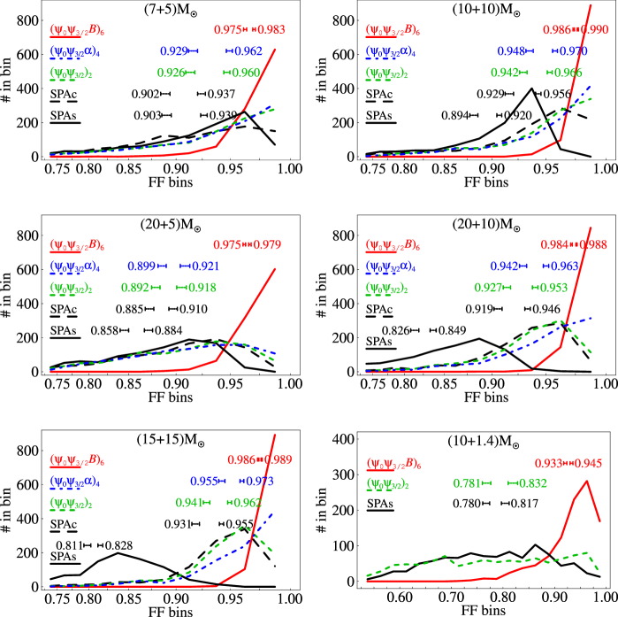
Figure 11: Distribution of fitting factor FF against the 2PN target model for the DTFs and for the standard SPA template families, for our BBH and NS–BH Monte Carlo populations. The vertices of the segmented curves show the number of samples (out of 1000) for which the FF falls within the equispaced bins $[0.725,0.75)$, $[0.75,0.775)$, … (the bins are plotted logarithmically to emphasize the region of FF close to one; notice that the NS–BH figure in the bottom right corner shows a different bin range). The vertical lines show the averages $\overline{\mathrm{FF}}$ and $\overline{\mathrm{FF}}_{\mathrm{eff}}$ with their $1\sigma$ error bars ($\overline{\mathrm{FF}}_{\mathrm{eff}}$ is always the larger number).

Table 8: Averages $\overline{\mathrm{FF}}$ and $\overline{\mathrm{FF}}_{\mathrm{eff}}$ of the fitting factor FF against the 2PN and 3.5PN target models, for the DTFs and for the standard SPA template families, as computed on our BBH Monte Carlo populations. The numbers in parentheses give the estimated Monte Carlo errors on the last two digits of $\overline{\mathrm{FF}}$ and $\overline{\mathrm{FF}}_{\mathrm{eff}}$.

Fitting factors against 3.5PN target model       $(7+5)M_{\odot}$       $(10+10)M_{\odot}$       $(15+15)M_{\odot}$       $(20+5)M_{\odot}$       $(20+10)M_{\odot}$       $\overline{\mathrm{FF}}$       $\overline{\mathrm{FF}}_{\mathrm{eff}}$       $\overline{\mathrm{FF}}$       $\overline{\mathrm{FF}}_{\mathrm{eff}}$       $\overline{\mathrm{FF}}$       $\overline{\mathrm{FF}}_{\mathrm{eff}}$       $\overline{\mathrm{FF}}$       $\overline{\mathrm{FF}}_{\mathrm{eff}}$       $\overline{\mathrm{FF}}$       $\overline{\mathrm{FF}}_{\mathrm{eff}}$    $(\psi_{0}\psi_{3/2}\mathcal{B})_{6}$ $0.9708(08)$ $0.9802(06)$ $0.9854(03)$ $0.9887(02)$ $0.9854(03)$ $0.9883(03)$ $0.9738(06)$ $0.9775(05)$ $0.9844(03)$ $0.9882(02)$

Table 9: Averages $\overline{\mathrm{FF}}$ and $\overline{\mathrm{FF}}_{\mathrm{eff}}$ of the fitting factor FF against the 2PN and 3.5PN target models, for the DTFs and for the standard SPA template families, as computed on the $(10+1.4)M_{\odot}$ NS–BH Monte Carlo populations. The numbers in parentheses give the estimated Monte Carlo errors on the last two digits of $\overline{\mathrm{FF}}$ and $\overline{\mathrm{FF}}_{\mathrm{eff}}$.

3.5PN target model    $(\psi_{0}\psi_{3/2}\mathcal{B})_{6}$ $0.9263(15)$ $0.9378(14)$

1. The SPA template families (solid and long-dashed black lines) always give the worst performance. Except for the lighter systems, $(7+5)M_{\odot}$ BBHs and $(10+1.4)M_{\odot}$ NS–BH binaries note44 , the SPAs family (solid black line) is consistently less effectual than SPAc, because the target-model ending frequencies are usually different from the Schwarzchild-ISCO frequencies used to terminate the SPAs templates (in the majority of cases, they are higher). The improvement [SPAs to SPAc] in $\overline{\mathrm{FF}}$ is $\simeq$ 3% for $M\simeq 20\mbox{--}25M_{\odot}$, and $\gtrsim$ 10% for $M=30M_{\odot}$. As pointed out in BCV1, it is important to add the frequency-cut parameter $f_{\mathrm{cut}}$ whenever the ending frequency is not known very well, but it is expected to fall within the band of good interferometer sensitivity.

2. Although the $(\psi_{0}\,\psi_{3/2})_{2}$ DTF (short-dashed green lines) is essentially a reparametrization of SPAc (both families have the $f_{\mathrm{cut}}$ parameter), it is slightly more effectual. The reason for this is that the physical ranges of $M$ and $\eta$ used to optimize FF (and in particular the constraint $\eta<0.25$) limit the ability of the expression $\psi_{\mathrm{SPA}}(f)$ to reproduce the phasing of the target. On the contrary, in the $(\psi_{0}\,\psi_{3/2})_{2}$ DTF the coefficients of $f^{-5/3}$ and $f^{-2/3}$ are not functions of $M$ and $\eta$, but free phenomenological parameters that can achieve the best possible values to match the target phasing. This added freedom does not buy a dramatic improvement for the spinning binaries studied in this paper, because the SPAc templates are already rather close to the adiabatic target model (except of course for precessional modulations). On the contrary, in BCV1 we saw that using unconstrained phenomenological parameters with extended ranges is very important to follow the nonadiabatic dynamics of late inspiral, as predicted by some PN models for nonspinning binaries.

3. The $(\psi_{0}\,\psi_{3/2}\,\alpha)_{4}$ DTF (dot-dashed blue lines) introduces the amplitude-remodeling coefficient $\alpha$. In BCV1 we found that $\alpha$ (together with the extension of parameter ranges) helped follow the nonadiabatic dynamics of some target PN models [see Tab. III.4]. In this paper, however, the only target model is obtained in the adiabatic limit, so the frequency-domain amplitude (except of course for the modulations due to precession) is always very close to the Newtonian expression $f^{-7/6}$. As a result, the improvement [$(\psi_{0}\,\psi_{3/2})_{2}$ to $(\psi_{0}\,\psi_{3/2}\,\alpha)_{4}$] in $\overline{\mathrm{FF}}$ is only $\simeq 0.3\mbox{--}1.6$%, while (at least according to the simple Gaussian analysis of Sec. V.2) the detection threshold increases by $\simeq$ 4% (although this number does not take into account the $\phi^{\alpha}=0$ constraint). It seems therefore that the $(\psi_{0}\,\psi_{3/2}\,\alpha)_{4}$ DTF is not a useful upgrade of $(\psi_{0}\,\psi_{3/2})_{2}$ for the purpose of detecting the signals emitted by precessing binaries.

4. The $(\psi_{0}\,\psi_{3/2}\,\mathcal{B})_{6}$ DTF [lighter–red solid lines] includes modulational corrections for both amplitude and phase. The resulting improvement in $\overline{\mathrm{FF}}$ over the SPA families is remarkable (for BBHs, 8–22% over SPAs, and 6–10% over SPAc; for NS–BH binaries, 20% over both). However, the effect of the modulational terms is seen best by comparing $(\psi_{0}\,\psi_{3/2}\,\mathcal{B})_{6}$ to $(\psi_{0}\,\psi_{3/2})_{2}$: we get an improvement of 5–9% for BBHs, and 20% for NS–BH binaries. This numbers should be compared with the projected increase $\simeq$ 8% in the detection threshold (Sec. V.2).

5. For the $(\psi_{0}\,\psi_{3/2}\,\mathcal{B}^{\prime})_{6}$ DTF, where the frequency dependence of the modulating terms is $f^{-2/3}$ rather than $f^{-1}$, fitting factors are not significantly different from $(\psi_{0}\,\psi_{3/2}\,\mathcal{B})_{6}$. Therefore we do not show these numbers. Tables VI.3 and VI.3 also contain a few FFs computed against the 3.5PN order target model (with $\widehat{\theta}=0$). The FFs, shown for the $(\psi_{0}\psi_{3/2}\mathcal{B})_{6}$ DTF, are essentially in line with their 2PN counterparts.

Table 10: Fitting factors against selected PN models of nonspinning binaries (see BCV1), for the SPAc and $(\psi_{0}\,\psi_{3/2}\,\alpha)_{4}$ template families. Notice that the $(\psi_{0}\,\psi_{3/2}\,\alpha)_{4}$ DTF yields consistently higher FFs.

Our results suggest two strategies to search for the signals from the precessing BBHs examined in this paper. We can try to follow the modulations induced by precession, using a DTF similar to $(\psi_{0}\,\psi_{3/2}\,\mathcal{B})_{6}$; or we can just use $(\psi_{0}\,\psi_{3/2})_{2}$, which is considerably better than SPAs (mostly because of $f_{\mathrm{cut}}$), and slightly better than SPAc (because of the extended parameter range). The gain in FF when we upgrade $(\psi_{0}\,\psi_{3/2})_{2}$ to $(\psi_{0}\,\psi_{3/2}\,\mathcal{B})_{6}$ is offset by a similar increase in the detection threshold, but the latter increase might be contained by reducing the range of the allowed $\alpha_{k}$, or by other data-analysis considerations that do come into the simple Gaussian analysis of Sec. V.2.

Figure 12 shows the projection of the 2PN target waveforms onto the $(\psi_{0},\psi_{3/2})$ section of the $(\psi_{0}\psi_{3/2})_{2}$ parameter space; Fig. 13 shows the projections of the waveforms onto the $(\psi_{0},\psi_{3/2})$ and $(\psi_{0},\mathcal{B})$ sections of the $(\psi_{0}\,\psi_{3/2}\,\mathcal{B})_{6}$ parameter space. It is interesting to notice that, with either strategy, the ranges of $\psi_{0}$ and $\psi_{3/2}$ needed to match effectually the signals in our populations are essentially the same found in BCV1 to match the signals predicted by a variety of PN models for BBHs without spins. In Figs. 12 and 13 these ranges are delimited by the thick dashed lines; the thin mass lines represent the range of detection templates needed to match effectually the signals predicted by different PN models for the same binary masses. As we can see, the projections of the spinning-binary signals are smeared around the nonspinning-binary mass lines with the same masses.

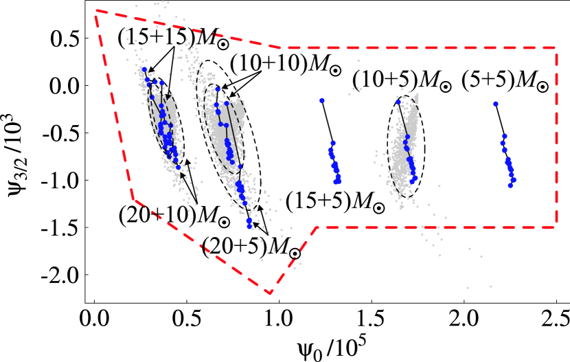
Figure 12: Projection of the 2PN target signals onto the $(\psi_{0}\,\psi_{3/2})_{2}$ DTF. For the $(10+10)M_{\odot}$, $(15+15)M_{\odot}$, $(20+5)M_{\odot}$, $(7+5)M_{\odot}$, and $(20+10)M_{\odot}$ BBHs in our Monte Carlo populations, the clusters of gray dots show the projection of the 2PN target waveforms onto the $(\psi_{0},\psi_{3/2})$ parameter plane of the $(\psi_{0}\,\psi_{3/2})_{2}$ DTF (the projection of a given target signal is given by the values of $\psi_{0}$ and $\psi_{3/2}$ that maximize the FF; here $f_{\mathrm{cut}}$ is not shown). For each set of masses, we draw a dashed ellipse centered on the parameter-space baricenter of the dots, and sized to include 90% of the dots (the proportions of the axes follow the two-dimensional quadratic moments of the dots). The larger blue dots, joined by the thin lines (mass lines), show the projections of the nonspinning PN models studied in BCV1, for the same sets of masses plus $(5+5)M_{\odot}$ and $(10+5)M_{\odot}$; each line joins signals with the same binary masses, but obtained from different PN target models. As we can see, for each set of masses, the projections of the spinning-binary signals are clustered around the corresponding mass line; moreover, all the projections fall within the region (delimited by the thick dashed lines) suggested in BCV1 to match all the nonspinning PN models.

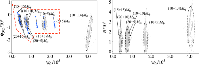
Figure 13: Projection of the 2PN target signals onto the $(\psi_{0}\,\psi_{3/2}\,\mathcal{B})_{6}$ DTF. For the $(10+10)M_{\odot}$, $(15+15)M_{\odot}$, $(20+5)M_{\odot}$, $(7+5)M_{\odot}$, and $(20+10)M_{\odot}$ BBHs, and for the $(10+1.4)M_{\odot}$ NS–BH binaries in our Monte Carlo populations, the clusters of gray dots show the projection of the 2PN target waveforms onto the $(\psi_{0},\psi_{3/2})$ [on the left] and $(\psi_{0},\mathcal{B})$ [on the right] parameter plane of the $(\psi_{0}\,\psi_{3/2}\,\mathcal{B})_{6}$ DTF. For each set of masses, we draw a dashed ellipse centered on the parameter-space baricenter of the dots, and sized to include 90% of the dots (the proportions of the axes follow the two-dimensional quadratic moments of the dots). The nonspinning-model mass lines and the boundary of the suggested parameter ranges are shown as in Fig. 12.

Thus, a signal search based on the $(\psi_{0}\,\psi_{3/2})_{2}$ DTF is a good starting point for both nonspinning and spinning binaries. It might also pay off, depending on the results of a more realistic evaluation of false-alarm probabilities, to upgrade this DTF to $(\psi_{0}\,\psi_{3/2}\,\alpha)_{4}$, with improved performance for nonspinning but nonadiabatic BBHs, as shown in BCV1; or even to $(\psi_{0}\,\psi_{3/2}\,\mathcal{B})_{6}$, with the best FFs for spinning binaries and without any deterioration for nonspinning ones.

VI.4 Modulated DTFs for NS–BH binaries

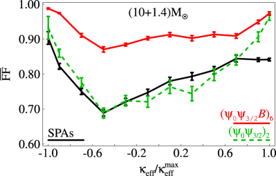
Figure 14: Average fitting factor for the DTFs and for the SPAs template families for $(10+1.4)M_{\odot}$ NS–BH binaries, plotted against the initial $\kappa_{\mathrm{eff}}=\hat{\mathbf{L}}_{N}\cdot\mathbf{S}_{\mathrm{eff}}$. The vertices of the segmented curves show the FF averaged on the sets of samples that fall within the equispaced $\kappa_{\mathrm{eff}}$ bins $[-1,-0.8)$, $[-0.8,-0.6)$, …, $[0.8,1]$. The error bars show the sampling error on the bin averages. We plot also two additional vertices, aligned with the abscissae $-1$ and $1$, which show the FF averaged over the $\kappa_{\mathrm{eff}}$ bins $[-1,-0.98)$ and $[0.98,1]$.

Let us now look in detail at the FFs achieved by the DTFs and standard template families against the signals generated by $(10+1.4)M_{\odot}$ NS–BH binaries where the BH is spinning rapidly (see Tab. VI.3 and Figs. 11 and 14). First of all, we notice that there is little difference between the performance of the SPAs and SPAc templates, because the ending frequency lies outside of the band of good interferometer sensitivity. Furthermore, the number of GW cycles within this band is very high, so it is crucial that a DTF reproduce very accurately the evolution of the GW phase; so using the $(\psi_{0}\,\psi_{3/2})_{2}$ DTF improves only slightly on the performance of the SPA templates. Introducing precessional corrections brings about a dramatic change: for the $(\psi_{0}\,\psi_{3/2}\,\mathcal{B})_{6}$ DTF, the increase in $\overline{\rm FF}$ and $\overline{\rm FF}_{\mathrm{eff}}$ with respect to SPA is respectively 20% and 16%, which is enough to justify the introduction of six $\alpha_{k}$ coefficients, according the Gaussian analysis of Sec. V.2.

The dependence of the FF on the spin configuration is shown in Fig. 14. For the NS–BH signals in our Monte Carlo population, Figs. 15 and 16 show the template parameters $\psi_{0}$, $\psi_{3/2}$, and $\mathcal{B}$ that maximize the overlap plotted against the initial $\kappa$ (conserved in NS–BH binaries). In the left panel, we see that the parameter $\psi_{0}$, which is related to the Newtonian chirp mass, has only a weak dependence on $\kappa$ (it varies by $\sim 8\%$); on the other hand, the parameter $\psi_{3/2}$ has a strong dependence. A plausible explanation is that the SO term in the SPA phasing is formally 1.5PN [see Eqs. (92) and (93)], and so is the term $\psi_{3/2}f$ in $\psi_{\mathrm{NM}}(f)$, which takes on the job, as it were, of reproducing the nonmodulational effects of the SO coupling. In the right panel, we see that for most of the binary configurations the values of $\mathcal{B}$ cluster around three lines [$\mathcal{B}=100$, $\mathcal{B}=(1+\kappa)\,110+110$, and $\mathcal{B}=(1+\kappa)\,240+160$]. Further analysis are needed to provide an explanation for this interesting behavior.

Thus, the $(\psi_{0}\,\psi_{3/2}\,\mathcal{B})_{6}$ DTF is a good candidate for the data-analysis problem of detecting GW signals from NS–BH binaries with rapidly spinning BHs. However, the analysis of precessional dynamics and GW emission carried out in this paper suggests an even more specialized DTF, which could be built with the following guidelines.

1. The waveform can be computed directly from Eq. (82) (obtained in the precessing convention): the necessary ingredients are the time evolution of the orbital phase $\Psi$ and of the binary polarization tensors $[\mathbf{e}_{+,\times}]_{ij}$, plus the fixed detector polarization tensors $[\mathbf{T}_{+,\times}]_{ij}$.

2. The evolution of $\Psi$ is obtained by solving Eq. (1), where $\mathbf{S}_{2}$ can be set to zero, and $\mathbf{S}_{1}$ enters only in the conserved term $\hat{\mathbf{L}}_{N}\cdot\mathbf{S}_{1}$. As a consequence, Eq. (1) is effectively uncoupled from the evolution of $\hat{\mathbf{L}}_{N}$, Eq. (9).

3. The evolution of the tensors $[\mathbf{e}_{+,\times}(t)]_{ij}$ is obtained from Eq. (71), after integrating Eqs. (2) and (9) for the coupled evolution of $\hat{\mathbf{L}}_{N}$ and $\mathbf{S}$, which depends only on $\hat{\mathbf{L}}_{N}\cdot\mathbf{S}_{1}$, on $S_{1}$ (conserved), and on $\omega(t)$.

4. A source frame attached to the initial configuration of the binary, similar to the frame constructed in Sec. IV.1 [see Eqs. (73)], can be used to carry out the explicit construction. By way of the initial conditions (74)–(77), the tensors $\mathbf{e}_{+,\times}$ and the orbital phase $\Psi$ (up to an additive constant $\Psi_{0}$) are then well defined as functions of the basic and local binary parameters only. We have therefore completed the specification of the first part of Eq. (82), which expresses the components of the mass quadrupole moment.

5. The remaining part of Eq. (82), which expresses the projection on the polarization tensor of the detector,

   $$P^{ij}\equiv[\mathbf{T}_{+}]^{ij}F_{+}+[\mathbf{T}_{\times}]^{ij}F_{\times},$$ (120)

   is determined by the directional parameters $\Theta$, $\varphi$, $\phi$, $\theta$, and $\psi$, which are now referred to the source frame attached to the binary. When we look for GWs using matched filtering, we can search rapidly over such a parametrization by treating the $P^{ij}$ as extrinsic parameters, along with the time of arrival and the initial orbital phase $\Psi_{0}$. The only intrinsic parameters would then be $m_{1}$, $m_{2}$, $S_{1}$, and $\mathbf{S}\cdot\hat{\mathbf{L}}_{N}$, all of which are conserved.

This family of templates adds a further intrinsic parameter with respect to $(\psi_{0}\,\psi_{3/2}\,\mathcal{B})_{6}$, but it has the advantage of producing essentially exact waveforms (valid in the adiabatic regime, and up to the highest PN order included), and of expressing these waveforms directly in terms of the physical spin parameters $S_{1}$ and $\mathbf{S}\cdot\hat{\mathbf{L}}_{N}$. We believe that the implementation and the false-alarm statistics of this family are worthy of further investigation BCV3 .

Figure 15: Projection of the $(10+1.4)M_{\odot}$ NS–BH target signals (computed at 2PN order) onto the $(\psi_{0}\,\psi_{3/2}\,\mathcal{B})_{6}$ DTF. The dots show the values of the $\psi_{0}$ (left panel) and $\psi_{3/2}$ (right panel) target parameters that yield maximum overlaps with the signals in the target populations.

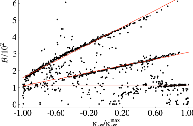
Figure 16: Projection of the $(10+1.4)M_{\odot}$ NS–BH target signals (computed at 2PN order) onto the $(\psi_{0}\,\psi_{3/2}\,\mathcal{B})_{6}$ DTF. The dots show the values of the $\mathcal{B}$ target parameter that yield maximum overlaps with the signals in the target populations.

VII Summary

In BCV1, the nonmodulated DTFs $(\psi_{0}\psi_{3/2})_{2}$ and $(\psi_{0}\psi_{3/2}\alpha)_{4}$ were shown to have FF $\gtrsim\,0.95$ against several nonspinning-BBH target models, obtained under different PN approximation schemes. In this paper, we have shown that these two families are also rather effectual at matching the signals from BH–BH and NS–BH precessing binaries with single-BH masses between 5 and 20 $M_{\odot}$ and with maximal BH spins, at least if these signals can be described by an adiabatic sequence of quasicircular orbits up to 2PN order.

More specifically, for $(7+5)M_{\odot}$, $(10+10)M_{\odot}$, $(20+10)M_{\odot}$, and $(15+15)M_{\odot}$ BBHs, we obtain $\overline{\mathrm{FF}}\gtrsim 0.93$ and $\overline{\mathrm{FF}}_{\mathrm{eff}}\gtrsim 0.95$. The improvement is 2–16% over Schwarzschild-terminated SPAs templates, thanks largely to the ending-frequency parameter $f_{\mathrm{cut}}$; and 1–2% over SPAc templates, thanks to the effective extension in the range of parameters, released from their functional dependence on the masses of the binary. Although the latter improvement seems negligible, we should keep in mind that $(\psi_{0}\,\psi_{3/2})_{2}$ DTFs are also more suitable to match the nonspinning BH binaries studied in BCV1 with PN expanded and resummed models. Results are worse for binaries that have smaller mass ratios $\eta$, and therefore more GW cycles in the band of good interferometer sensitivity. In this case the modulational effects due to precession become important, and must be included in the detection templates. Indeed, for $(20+5)M_{\odot}$ BBHs, the $(\psi_{0}\psi_{3/2})_{2}$ and $(\psi_{0}\psi_{3/2}\alpha)_{4}$ DTFs have $\overline{\mathrm{FF}}\simeq 0.89$ and $\overline{\mathrm{FF}}_{\mathrm{eff}}\simeq 0.92$; for a $(10+1.4)M_{\odot}$ NS–BH binary, we find $\overline{\mathrm{FF}}\simeq 0.78$, and $\overline{\mathrm{FF}}_{\mathrm{eff}}\simeq 0.83$.

Motivated by these shortcomings, we have investigated in detail the dynamics of precession in these binaries, and we have introduced a new convention to write the GW signal (as computed in the quadrupole approximation) as a function of binary and detector parameters, isolating the oscillatory effects of precession in the evolution of the polarization tensors $[\mathbf{e}_{+,\times}]_{ij}$. As a result, the detector response to GWs can be written as the product of a carrier signal, which very closely resembles the nonspinning signals studied in BCV1, and a modulational correction, which can be handled using an extension of Apostolatos’ ansatz (64). On the basis of these observations, we build the modulated DTF $(\psi_{0},\psi_{3/2}\mathcal{B})_{6}$, which yields $\overline{\mathrm{FF}}$ and $\overline{\mathrm{FF}}_{\mathrm{eff}}\simeq$ 0.98–0.99 for the BBHs investigated, and $\overline{\mathrm{FF}}\simeq 0.93$, $\overline{\mathrm{FF}}_{\mathrm{eff}}\simeq 0.95$ for $(10+1.4)M_{\odot}$ NS–BH binaries. This DTF has the advantage that all the modulational parameters (except for $\mathcal{B}$) can be treated as extrinsic parameters, reducing considerably the computational cost of signal searches. According to the simple analysis of Sec. V.2, the detection thresholds for this DTF should be set higher than those for simpler families; still, the gain in FF is still somewhat larger than the increase in the threshold, and more realistic analyses of false-alarm statistics might provide a way to sidestep this difficulty. The same arguments that lead to the $(\psi_{0},\psi_{3/2}\mathcal{B})_{6}$ DTF suggest a new, very promising class of templates for NS–BH binaries, which we discuss briefly in Sec. VI.4, and which we plan to investigate more thoroughly elsewhere BCV3 .

We wish to make a few final remarks. First, in this paper we limited our analysis to compact objects moving on quasicircular orbits; from the results on the ending frequencies (see Fig. 5) we see that there exist spin initial conditions for which the ending frequencies (end of inspiral) are in the LIGO–VIRGO band. So, in these cases we should use spinning dynamics that goes beyond the adiabatic approximation. This dynamics (without radiation-reaction effects) is already available in the EOB framework BD ; EOB3PN thanks to the work of Damour TD . We plan to investigate the effects of nonadiabatic PN dynamics in the near future.

Second, a few years ago Levin pointed out JL that spin-spin effects can introduce chaos into the trajectories; as a consequence, the gravitational waveforms would come to depend sensitively on the initial conditions. More studies followed SR ; CL . Considering only conservative dynamics (no RR), Cornish and Levin CL found some examples of rather eccentric ($e\sim 0.6$ or $0.9$) chaotic orbits, and a few quasicircular chaotic orbits. However, these authors observed that chaos would be damped by RR effects, and that it would not affect the inspiral waveforms, except (perhaps) at the very end (the plunge). Still, at this time the dynamical structure of phase space has not been explored systematically, and a more conclusive study tuned to the LIGO–VIRGO detection problem remains desirable. The analysis of this paper assumes that, by the time the GW signal enters the band of good detector sensitivity, RR effects have circularized the orbit, and have brought the binary into the adiabatic regime, which is valid until the MECO. We did not try to perturb the initial conditions slightly and to investigate the resulting changes in the orbital evolution and in the waveforms.

Third, we have evaluated the performance of our DTFs by averaging over uniform distributions of the initial spin angles. Of course it would be preferable to assume more realistic, nonuniform distributions derived from astrophysical considerations. Some results for spin distributions in BBHs (with only one spinning BH), and in NS–BH binaries were obtained by Kalogera using population-synthesis techniques VK . In particular, Kalogera found that $30\mbox{--}80\%$ of the NS–BH binaries that will coalesce within a Hubble time can have a tilt angle (the angle between the spin and the orbital angular momentum) larger than $30$ degrees. These results assume that the spinning BH in the binary forms first, and that its spin is aligned with the orbital angular momentum; the tilt angle originates from the supernova explosion that forms the NS. For the case of the binaries formed in globular clusters, there is no theoretical argument to suggest any particular spin distribution.

Finally, recent analyses of spin-spin effects in the PN inspiral equations JS suggest that, for comparable-mass BBHs, by the time the GW signal enters the band of good interferometer sensitivity the two BH spins may have become roughly locked into a fixed relative configuration. If these results are confirmed, they could provide preferred initial spin conditions, and simplify the data-analysis problem for comparable mass binaries, by reducing the variability of expected GW signals.

Appendix A Validity of the adiabatic sequence of spherical orbits

In the target model defined in Sec. II.1, the inspiral of the two compact bodies is described as an adiabatic sequence of spherical orbits. In this Appendix we wish to discuss the validity of this assumption. Introducing the orthonormal basis $(\hat{\mathbf{\lambda}},\hat{\mathbf{n}},\hat{\mathbf{L}}_{N})$, where $\hat{\mathbf{n}}=\mathbf{x}/r$, $\hat{\mathbf{L}}_{N}=\mathbf{L}_{N}/L_{N}$, $\hat{\mathbf{\lambda}}=\hat{\mathbf{L}}_{N}\times\hat{\mathbf{n}}$ and $\mathbf{L}_{N}=\mu\,\mathbf{x}\times\mathbf{v}$ (with $\mu$ the reduced mass), it is straightforward to write the equations of motion as [see Eqs. (4.1) of Ref. K ; we use the relations $\mathbf{v}=\dot{r}\,\hat{\mathbf{n}}+r\,\omega\,\hat{\mathbf{\lambda}},v^{2}=\dot{r}^{2}+r^{2}\,\omega^{2}$]:

$$\hat{\mathbf{n}}\cdot\mathbf{a} = \ddot{r}-r\,\omega^{2}\,,$$ (121)

$$\hat{\mathbf{\lambda}}\cdot\mathbf{a} = r\,\dot{\omega}+2\dot{r}\,\omega\,,$$ (122)

$$\hat{\mathbf{L}}_{N}\cdot\mathbf{a} = -r\,\omega\,\frac{d\hat{\mathbf{L}}_{N}}{dt}\cdot\hat{\mathbf{\lambda}}\,,$$ (123)

where $\mathbf{a}$ is the acceleration in harmonic gauge given by Eqs. (2.2a), (2.2c) of Ref. K . If we impose $\dot{r}=0=\ddot{r}$, Eq. (122) then implies $\dot{\omega}=0$; and from Eq. (121) we get

$$r^{2}\,\omega^{2}=\frac{1}{r}\,\left(1-\frac{2}{r^{2}}\,\mathbf{L}_{N}\cdot\mathbf{S}_{\omega}\right)\,,\quad\quad\mathbf{S}_{\omega}\equiv\left(1+\frac{3}{2}\,\frac{m_{2}}{m_{1}}\right)\,\mathbf{S}_{1}+\left(1+\frac{3}{2}\,\frac{m_{1}}{m_{2}}\right)\,\mathbf{S}_{2}\,,$$ (124)

where for simplicity we have set $M=1$. Although spherical orbits (orbits where both $r$ and $\omega$ remain constant) exist at any given instant, they are not preserved along dynamical evolution because the quantity $\mathbf{L}_{N}\cdot\mathbf{S}_{\omega}$ that appears in Eq. (124) is not conserved. Indeed, averaging over an orbit note38 (and, for simplicity, neglecting spin-spin effects), we get

$$\left\langle\frac{d\mathbf{L}_{N}}{dt}\right\rangle=\frac{2\mu}{r^{3}}\mathbf{S}_{\rm eff}\times\mathbf{L}_{N}\,,\quad\quad\mathbf{S}_{\rm eff}\equiv\left(1+\frac{3}{4}\,\frac{m_{2}}{m_{1}}\right)\,\mathbf{S}_{1}+\left(1+\frac{3}{4}\,\frac{m_{1}}{m_{2}}\right)\,\mathbf{S}_{2}\,,$$ (125)

where $\langle A\rangle$ denotes the quantity $A$ when the spin-orbit (and spin-spin) terms have been averaged over an orbit. Using the precession equations for the spins we derive

$$\left\langle\frac{d(\mathbf{L}_{N}\cdot\mathbf{S}_{\omega})}{dt}\right\rangle=-3\frac{(m_{1}^{2}-m_{2}^{2})}{m_{1}\,m_{2}}\,\mathbf{L}_{N}\cdot(\mathbf{S}_{1}\times\mathbf{S}_{2})\,\frac{1}{r^{3}}\,.$$ (126)

Hence, because the circular-orbit condition is not preserved during the evolution, either $\langle\dot{\omega}\rangle\neq 0$ or $\langle\dot{r}\rangle\neq 0$ (or both).

Let us now see how Eq. (1) for $\dot{\omega}$ changes if effects of this kind are included. The usual argument K ; KWW used to obtain the adiabatic evolution of $\omega$ rests on the energy-balance equation,

$$\dot{E}_{\rm RR}=\frac{d}{dt}E(\omega,\hat{\mathbf{L}}_{N},\mathbf{S}_{1},\mathbf{S}_{2})=\frac{\partial E}{\partial\omega}\dot{\omega}+\left(\frac{\partial E}{\partial\hat{\mathbf{L}}_{N}}\cdot\dot{\hat{\mathbf{L}}}_{N}+\frac{\partial E}{\partial\mathbf{S}_{1}}\cdot\dot{\mathbf{S}_{1}}+\frac{\partial E}{\partial\mathbf{S}_{2}}\cdot\dot{\mathbf{S}_{2}}\right)\,,$$ (127)

where

$$E(\omega,\hat{\mathbf{L}}_{N},\mathbf{S}_{1},\mathbf{S}_{2})=-\frac{\mu}{2}\,(M\omega)^{2/3}\,\Bigg{\{} 1 -\frac{(9+\eta)}{12}\,(M\omega)^{2/3}+\frac{8}{3M^{2}}\hat{\mathbf{L}}_{N}\cdot\mathbf{S}_{\rm eff}\,(M\omega)+$$

$$\bigg{[}\frac{1}{24}(-81+57\eta-\eta^{2})+\frac{1}{\eta M^{4}}\left[(\mathbf{S}_{1}\cdot\mathbf{S}_{2})-3(\hat{\mathbf{L}}_{N}\cdot\mathbf{S}_{1})(\hat{\mathbf{L}}_{N}\cdot\mathbf{S}_{2})\right]\bigg{]}(M\omega)^{4/3}\Bigg{\}}$$

is the orbital energy evaluated at Newtonian order, but including spin-orbit and spin-spin effects, and where $\dot{E}_{\rm RR}$ is the RR energy loss KWW ; K . From Eqs. (A), (9), (2) and (3), we notice that the sum of the last three terms in parentheses in Eq. (127) does not vanish: at leading order, its value is

$$\dot{E}_{\rm extra}=\frac{1}{4}\frac{(m_{1}-m_{2})}{M}\,\eta^{2}\,\chi_{1}\,\chi_{2}\,(M\omega)^{11/3}\,\left[\left(\hat{\mathbf{S}}_{1}\times\hat{\mathbf{S}}_{2}\right)\cdot\hat{\mathbf{L}}_{N}\right]\,.$$ (129)

This expression is zero if masses are equal, or if spins are either aligned or antialigned. Retaining the term (129) in the calculation yields an additional contribution in the evolution of $\omega$, with a leading order correction

$$\frac{\dot{\omega}_{\rm extra}}{\omega^{2}}=\frac{3}{4}\frac{(m_{1}-m_{2})}{M}\,\eta\,\chi_{1}\,\chi_{2}\,(M\omega)^{2}\,\left[\left(\hat{\mathbf{S}}_{1}\times\hat{\mathbf{S}}_{2}\right)\cdot\hat{\mathbf{L}}_{N}\right]\,.$$ (130)

Thus, compared with the other terms in Eq. (1), $\dot{\omega}_{\rm extra}$ appears formally at 0.5 PN order (very low!) in the expansion of $\dot{\omega}$. Note that the spin-orbit term in the energy (A), combined with the leading-order precessions, does not produce such a term; this makes the adiabatic approach fully consistent up to 1.5PN order. In fact, $\dot{E}_{\rm extra}$ originates from taking the derivative of $\dot{E}_{\rm SO}$ and using next-to-leading order terms in the precession equations, and the derivative $\dot{E}_{\rm SS}$ while using the leading-order terms in the precession equations.

However, the effect of this term in the regime that we consider is not as large as suggested by its formal PN order. For example, under the worst possible assumption (that the geometric factor $[(\hat{\mathbf{S}}_{1}\times\hat{\mathbf{S}}_{2})\cdot\hat{\mathbf{L}}_{N}]$ has always the maximum value of one, and that spins are maximal), we get the correction

$$\frac{\Delta\Psi_{\rm extra}}{2\pi}=\frac{1}{2\pi}\,\frac{25}{16384}\,\frac{\sqrt{1-4\eta}}{\eta}\,\left[(M\omega_{f})^{-4/3}-(M\omega_{i})^{-4/3}\right]$$ (131)

to the number of orbital cycles, where $\omega_{i}$ and $\omega_{f}$ are the initial and final orbital frequencies under consideration. This is formally a 0.5PN correction, as can be seen by comparing it with Eq. (4.16) of Ref. K . Nevertheless, for (say) a $(20+5)M_{\odot}$ BBH, this correction will be at most $0.34$ orbital cycles from $\omega_{i}=\pi\times 30$ Hz to $\omega_{i}=\pi\times 400$ Hz, to be compared with a baseline of $52$ orbital cycles from the Newtonian term and $8$ from the 1PN term. For a $(10+1.4)M_{\odot}$ binary, the correction will be $1.6$ orbital cycles, to be compared with $175$ orbital cycles from the Newtonian term and $30$ from the 1PN term. The correction is small because, although the PN order is formally low, the numerical coefficient of the geometric factor $[(\hat{\mathbf{S}}_{1}\times\hat{\mathbf{S}}_{2})\cdot\hat{\mathbf{L}}_{N}]$ is very small.

So far, we have assumed $[(\hat{\mathbf{S}}_{1}\times\hat{\mathbf{S}}_{2})\cdot\hat{\mathbf{L}}_{N}]\sim 1$ along the evolution. Let us now estimate the more important effect that comes from the precession of $\hat{\mathbf{L}}_{N}$, $\mathbf{S}_{1}$ and $\mathbf{S}_{2}$, which is especially important for binaries with small mass ratios, which have longer RR time scales and more precessional cycles. At the leading order (with $M=1$)

$$\frac{d}{dt}\left[\left(\hat{\mathbf{S}}_{1}\times\hat{\mathbf{S}}_{2}\right)\cdot\hat{\mathbf{L}}_{N}\right]=\frac{3}{2}(m_{1}-m_{2})\,\omega^{5/3}\,\left[\hat{\mathbf{S}}_{1}\cdot\hat{\mathbf{S}}_{2}-(\hat{\mathbf{S}}_{1}\cdot\hat{\mathbf{L}}_{N})\,(\hat{\mathbf{S}}_{2}\cdot\hat{\mathbf{L}}_{N})\right]+{\cal O}(\omega^{2})\,,$$ (132)

and

$$\frac{d}{dt}\left[\hat{\mathbf{S}}_{1}\cdot\hat{\mathbf{S}}_{2}-(\hat{\mathbf{S}}_{1}\cdot\hat{\mathbf{L}}_{N})(\hat{\mathbf{S}}_{2}\cdot\hat{\mathbf{L}}_{N})\right]=-\frac{3}{2}(m_{1}-m_{2})\,\omega^{5/3}\left[\left(\hat{\mathbf{S}}_{1}\times\hat{\mathbf{S}}_{2}\right)\cdot\hat{\mathbf{L}}_{N}\right]+{\cal O}(\omega^{2})\,.$$ (133)

Combining the above equations, we get (at leading order)

$$\frac{d^{2}}{dt^{2}}\left[\left(\hat{\mathbf{S}}_{1}\times\hat{\mathbf{S}}_{2}\right)\cdot\hat{\mathbf{L}}_{N}\right]\simeq-\frac{9}{4}(m_{1}-m_{2})^{2}\,\omega^{10/3}\,\left[\left(\hat{\mathbf{S}}_{1}\times\hat{\mathbf{S}}_{2}\right)\cdot\hat{\mathbf{L}}_{N}\right]\,.$$ (134)

This means that the geometric factor $[(\hat{\mathbf{S}}_{1}\times\hat{\mathbf{S}}_{2})\cdot\hat{\mathbf{L}}_{N}]$ oscillates around zero with a time scale $\sim\omega^{-5/3}$. Thus the effect of $\dot{\omega}_{\rm extra}$ accumulates only within this timescale, which is 1.5 PN orders shorter than the RR timescale. Therefore, we expect that the real $\Delta\Psi_{\rm extra}$ will be even smaller than the formal prediction given by Eq. (131), and that it will contribute effectively at 2PN order. As a check, we evaluated the FF between the gravitational waveforms obtained, for a $(10+1.4)M_{\odot}$ binary, by first including and then dropping the extra term in $\dot{\omega}$. We found that the FF is $\simeq 0.99$. On the basis of this last check and of the analysis outlined above, we conclude that the adiabatic assumption is quite adequate for the purposes of this paper.

Appendix B Proof that the precessing convention yields $\omega=\dot{\Phi}_{S}$

First of all, it is easy to confirm that, as long as $\mathbf{e}_{1,2}(0)$ and $\hat{\mathbf{L}}_{N}(0)$ form an orthonormal basis at some initial time, the evolution equation $\dot{\mathbf{e}}_{1,2}=\mathbf{\Omega}_{e}\times\mathbf{e}_{1,2}$ will always keep the triplet an orthonormal basis. It is then always possible to have a $\Phi(t)$, such that

$$\hat{\mathbf{n}}(t)=\mathbf{e}_{1}\cos\Phi(t)+\mathbf{e}_{2}\sin\Phi(t)\,,\quad\hat{\mathbf{\lambda}}(t)=-\mathbf{e}_{1}\sin\Phi(t)+\mathbf{e}_{2}\cos\Phi(t)\,.$$ (135)

Taking the time derivative of $\hat{\mathbf{n}}(t)$, we have

$$\dot{\hat{\mathbf{n}}}=\dot{\Phi}\hat{\mathbf{\lambda}}+\mathbf{\Omega}_{e}\times\hat{\mathbf{n}}$$ (136)

Now, the adiabatic condition for a sequence of circular orbits states that $\dot{\hat{\mathbf{n}}}=\omega\hat{\mathbf{\lambda}}$, so we have

$$\dot{\hat{\mathbf{n}}}=\omega\hat{\mathbf{\lambda}}=\dot{\Phi}\hat{\mathbf{\lambda}}+\mathbf{\Omega}_{e}\times\hat{\mathbf{n}}.$$ (137)

By definition [Eq. (72)], $\mathbf{\Omega}_{e}$ has no components along $\mathbf{e}_{3}\equiv\hat{\mathbf{L}}_{N}$. It also has no components along $\hat{\mathbf{\lambda}}$, because

$$\mathbf{\Omega}_{e}\times\hat{\mathbf{L}}_{N} = \dot{\hat{\mathbf{L}}}_{N}=\dot{\hat{\mathbf{n}}}\times\hat{\mathbf{\lambda}}+\hat{\mathbf{n}}\times\dot{\hat{\mathbf{\lambda}}}=\omega\hat{\mathbf{\lambda}}\times\hat{\mathbf{\lambda}}+\hat{\mathbf{n}}\times(-\dot{\Phi}\hat{\mathbf{n}}+\mathbf{\Omega}_{e}\times\hat{\mathbf{\lambda}})$$ (138)

$$= \mathbf{\Omega}_{e}(\hat{\mathbf{n}}\cdot\hat{\mathbf{\lambda}})-\hat{\mathbf{\lambda}}(\hat{\mathbf{n}}\cdot\mathbf{\Omega}_{e})\propto\hat{\mathbf{\lambda}},$$ (139)

where in the last step we used $\hat{\mathbf{n}}\cdot\hat{\mathbf{\lambda}}=0$ and the vector–triple-product rule. It follows that $\mathbf{\Omega}_{e}$ lies along $\hat{\mathbf{n}}$, and therefore $\mathbf{\Omega}_{e}\times\hat{\mathbf{n}}=0$. Equation (137) then gives the desired result, $\dot{\Phi}=\omega$, i.e. $\Phi(t)=\Psi(t)+\mathrm{const}$.

References

- (1) A. Abramovici et al., Science 256, 325 (1992); B. Caron et al., Class. Quantum Grav. 14, 1461 (1997); H. Lück et al., Class. Quantum Grav. 14, 1471 (1997); M. Ando et al., Phys. Rev. Lett. 86, 3950 (2001).
- (2) B. S. Sathyaprakash and S. V. Dhurandhar, Phys. Rev. D 44, 3819 (1991); L. S. Finn, Phys. Rev. D 46, 5236 (1992); S. V. Dhurandhar and B. S. Sathyaprakash, Phys. Rev. D 49, 1707 (1994); B. S. Sathyaprakash, Phys. Rev. D 50, R7111 (1994); C. Cutler and É. É. Flanagan, Phys. Rev. D 49, 2658 (1994); B. J. Owen, Phys. Rev. D 53, 6749 (1996); B. J. Owen and B. Sathyaprakash, Phys. Rev. D 60, 022002 (1999); É. É. Flanagan and S. A. Hughes, Phys. Rev. D 57, 4535 (1998); ibid., 4566 (1998); T. Damour, B. R. Iyer and B. S. Sathyaprakash, Phys. Rev. D 62, 084036 (2000); F. A. Jenet and T. Prince, Phys. Rev. D 62, 122001 (2000); A. E. Chronopoulos and T. A. Apostolatos, Phys. Rev. D 64, 042003 (2001); E. Porter, Class. Quant. Grav. 19, 4343 (2002).
- (3) T. Damour, B. R. Iyer and B. S. Sathyaprakash, Phys. Rev. D 57, 885 (1998).
- (4) A. Buonanno and T. Damour, Phys. Rev. D 59, 084006 (1999); 62, 064015 (2000).
- (5) T. Damour, P. Jaranowski and G. Schäfer, Phys. Rev. D 62, 084011 (2000).
- (6) T. Damour, 300 Years of Gravitation, S. W. Hawking and W. Israel, eds. (Cambridge University Press, Cambridge, England, 1987); L. Blanchet, Living Reviews in Relativity, 2002-3 (2002), http://www.livingreviews.org/Articles/Volume5/2002-3blanchet.
- (7) T. Damour, B. R. Iyer and B. S. Sathyaprakash, Phys. Rev. D 63, 044023 (2001); 66, 027502 (2002).
- (8) BCV1: A. Buonanno, Y. Chen and M. Vallisneri, Phys. Rev. D 67, 024016 (2003).
- (9) T. Damour, B. R. Iyer, P. Jaranowski and B. S. Sathyaprakash, Phys.Rev. D 67, 064028 (2003).
- (10) T. A. Apostolatos, C. Cutler, G. J. Sussman and K. Thorne, Phys. Rev. D 49, 49 (1994).
- (11) T. A. Apostolatos, Phys. Rev. D 54, 2438 (1996).
- (12) P. Grandclément, V. Kalogera and A. Vecchio, Phys. Rev. D 67, 042003 (2003).
- (13) P. Grandclément and V. Kalogera, Phys. Rev. D, in print (2003).
- (14) T. Damour, Phys. Rev. D 64, 124013 (2001).
- (15) L. S. Finn and D. F. Chernoff, Phys. Rev. D 47, 2198 (1993).
- (16) L. E. Kidder, Phys. Rev. D 52, 821 (1995).
- (17) L. Blanchet, T. Damour, B. R. Iyer, C. M. Will and A. G. Wiseman, Phys. Rev. Lett. 74, 3515 (1995); L. Blanchet, T. Damour and B. R. Iyer, Phys. Rev. D 51, 536 (1995); C. M. Will and A. G. Wiseman, Phys. Rev. D 54, 4813 (1996).
- (18) L. Blanchet, B. R. Iyer, C. M. Will and A. G. Wiseman, Class. Quantum Grav. 13, 575 (1996).
- (19) L. Blanchet, Phys. Rev. D 54, 1417 (1996); L. Blanchet, Class. Quantum Grav. 15, 113 (1998).
- (20) L. Blanchet, G. Faye, B. R. Iyer, B. Joguet, Phys. Rev. D 65, 061501 (2002); L. Blanchet, B. R. Iyer and B. Joguet, Phys. Rev. D 65, 064005 (2002).
- (21) L. E. Kidder, C.M. Will and A.G. Wiseman, Phys. Rev. D 47, 4183 (R) (1993).
- (22) T. Damour, P. Jaranowski and G. Schäfer, Phys. Lett. B 513, 147 (2001).
- (23) P. Jaranowski and G. Schäfer, Phys. Rev. D 57, 7274 (1998); ibid. 60, 124003 (1999); T. Damour, P. Jaranowski and G. Schäfer, Phys. Rev. D 62, 044024 (2000); ibid., 021501(R) (2000); 63, 044021 (2001).
- (24) Note that the MECO, as defined by Eq. (13) via a total derivative, depends also on the evolution of , and . However, later in this paper (Sec. III.2) we shall see that this dependence is rather weak.
- (25) L. Blanchet, Phys. Rev. D 65, 124009 (2002).
- (26) N. Wex, Class. Quantum Grav. 12, 983 (1995).
- (27) When referring to results at 3PN and 3.5PN orders we shall always set the arbitrary parameter in Eq. (1). In the nonspinning case, the dependence of the GW signal on is rather mild, at least if is limited to values of order one BFIJ , as investigated in BCV1.
- (28) É. É. Flanagan and S. A. Hughes, Phys. Rev. D 57, 4535 (1998).
- (29) Here “quadrupole” refers to the multipolar expansion used to compute GWs, and not to the expansion used to introduce RR effects in the inspiral.
- (30) T. A. Apostolatos, Phys. Rev. D 52, 605 (1995).
- (31) Because the amplitude of signals is generally unknown, the FF is generally defined in terms of normalized signals in the sense of Eq. (98).
- (32) B. F. Schutz, in The Detection of Gravitational Radiation, D. Blair, ed. (Cambridge University Press, Cambridge, England, 1989).
- (33) W. H. Press, S. A. Teukolsky, W. T. Vetterling and B. P. Flannery, Numerical recipes in C: the art of scientific computing (Cambridge University Press, Cambridge, England, 1992).
- (34) The time of arrival of the GW signal is an extrinsic parameter (it is searched automatically for the best possible value using FFT integrals); however, when we evaluate the total false-alarm probability it is easier to consider a single detection test for each possible time of arrival. So the probability distributions discussed in Sec. V.2 are for an overlap statistic that is not automatically maximized over the time of arrival.
- (35) B. Allen et al., Phys. Rev. Lett. 83, 1498 (1999).
- (36) R. G. Miller, Biometrika 61, 1 (1974).
- (37) The downward-arcing envelope of Fig. 10b actually corresponds to , possibly because the ending frequency (a function of ) plays into SA.
- (38) Because the template family SPAs is a subset of SPAc, SPAs should always be more effectual. In fact, for BBHs and NS–BH binaries, we find slightly higher numbers for SPAs. In these lighter systems, SPAc has no advantage over SPAs because the ending frequency is above the range of good detector sensitivity, so the FFs should be the same. However, evaluating the effectualness of SPAc requires a three-parameter numerical maximization of the overlap, which is inevitably less precise than the two-parameter maximization needed for SPAs. So numerical error explains the discrepancy.
- (39) A. Buonanno, Y. Chen, Y. Pan, and M. Vallisneri, in preparation.
- (40) J. Levin, Phys. Rev. Lett. 84, 3515 (2000); J. Levin, Phys. Rev. D 67, 044013 (2003).
- (41) J. D. Schnittman and F. Rasio, Phys. Rev. Lett. 87, 121101 (2001).
- (42) N. J. Cornish and J. Levin, gr-qc/0207016; N. J. Cornish and J. Levin, Phys. Rev. Lett. 89, 179001 (2002).
- (43) V. Kalogera, Astrophysical Journal 541, 319 (2000).
- (44) J. D. Schnittman, private communication; “Spin-Orbit Resonance in Compact Binary LIGO Sources”, talk given at LSC workshop, Hanford, August 2002.
- (45) We are implicitly assuming that the precession frequency is much smaller than both the orbital frequency and the effective radiation-reaction frequency , where is the radiation-reaction folding time.
- (46) L. Blanchet, B. R. Iyer, and B. Joguet, Phys. Rev. D 71, 129902(E) (2005); 71, 129903(E) (2005); L. Blanchet, ibid. 71, 129904(E) (2005).
- (47) L. Blanchet, T. Damour, G. Esposito-Farèse, and B. R. Iyer, Phys. Rev. Lett. 93, 091101 (2004).