Abstract

A new implementation for magnetohydrodynamics (MHD) simulations in full general relativity (involving dynamical spacetimes) is presented. In our implementation, Einstein’s evolution equations are evolved by a BSSN formalism, MHD equations by a high-resolution central scheme, and induction equation by a constraint transport method. We perform numerical simulations for standard test problems in relativistic MHD, including special relativistic magnetized shocks, general relativistic magnetized Bondi flow in stationary spacetime, and a longterm evolution for self-gravitating system composed of a neutron star and a magnetized disk in full general relativity. In the final test, we illustrate that our implementation can follow winding-up of the magnetic field lines of magnetized and differentially rotating accretion disks around a compact object until saturation, after which magnetically driven wind and angular momentum transport inside the disk turn on.

I Introduction

Hydrodynamics simulation in general relativity is probably the best theoretical approach for investigating dynamical phenomena in relativistic astrophysics such as stellar core collapse to a neutron star and a black hole, and the merger of binary neutron stars. In the past several years, this field has been extensively developed (e.g., [1, 2, 3, 4, 5, 6, 7]) and, as a result, now it is feasible to perform accurate simulations of such general relativistic phenomena for yielding scientific results (e.g., [6, 7, 8, 9] for our latest results). For example, with the current implementation, radiation reaction of gravitational waves in the merger of binary neutron stars can be taken into account within $\sim 1\%$ error in an appropriate computational setting [6, 7]. This fact illustrates that the numerical relativity is a robust approach for detailed theoretical study of astrophysical phenomena and gravitational waves emitted.

However, so far, most of the scientific simulations in full general relativity have been performed without taking into account detailed effects except for general relativistic gravity and pure hydrodynamics. For example, simplified ideal equations of state have been adopted instead of realistic ones (but see [7]). Also, the effect of magnetic fields has been neglected although it could often play an important role in the astrophysical phenomena (but see [10]). In the next stage of numerical relativity, it is necessary to incorporate these effects for more realistic simulations. As a step toward a more realistic simulation, we have incorporated an implementation for ideal magnetohydrodynamics (MHD) equations in fully general relativistic manner. In this paper, we describe our approach for these equations and then present numerical results for test problems computed by the new implementation.

Magnetic fields indeed play an important role in determining the evolution of a number of relativistic objects. In the astrophysical context, the plasma is usually highly conducting, and hence, the magnetic fields are frozen in the matter. This implies that a small seed field can wind up and grow in the complex motion of the matter, resulting in a significant effect in the dynamics of the matter such as magnetically driven wind or jet and angular momentum redistribution. Specifically, in the context of the general relativistic astrophysics, the magnetic fields will play a role in the following phenomena and objects: Stellar core collapse of magnetized massive stars to a protoneutron star [11] or a black hole, stability of accretion disks (which are either non-self-gravitating or self-gravitating) around black holes and neutron stars, magnetic braking of differentially rotating neutron stars [10] which are formed after merger of binary neutron stars [6, 7] and stellar core collapse [14, 15, 16, 8, 9], and magnetically induced jet around the compact objects (e.g., [17]). To clarify these phenomena, fully general relativistic MHD (GRMHD) simulation (involving dynamical spacetimes) is probably the best theoretical approach.

In the past decade, numerical implementations for GRMHD simulation in the fixed gravitational field have been extensively developed (e.g., [18, 17, 19, 20, 21, 22, 23, 24]). In particular, it is worth to mention that Refs. [19, 20, 21, 22, 23] have recently presented implementations for which detailed tests have been carried out for confirmation of the reliability of their computation, in contrast with the attitude in an early work [17]. They are applied for simulating magnetorotational instability (MRI) of accretion disks and subsequently induced winds and jets around black holes and neutron stars. On the other hand, little effort has been paid to numerical implementations of fully GRMHD (in the dynamical gravitational field). About 30 years ago, Wilson performed a simulation for collapse of a magnetized star in the presence of poloidal magnetic fields in general relativity. However, he assumes that the three-metric is conformally flat [25], and hence, the simulation is not fully general relativistic, although recent works have indicated that the conformally flat approximation works well in the axisymmetric collapse (e.g., compare results among [15], [26], and [27]). The first fully GRMHD simulation for stellar collapse was performed by Nakamura about 20 years ago [28]. He simulated collapse of nonrotating stars with poloidal magnetic fields to investigate the criteria for formation of black holes and naked singularities. Very recently, Duez et al. have presented a new implementation capable of evolution for the Einstein-Maxwell-MHD equations for general cases [10]. They report successful results for test simulations. Valencia group has also developed a GRMHD implementation very recently [29].

In this paper, we present our new implementation for fully GRMHD which is similar to but in part different from that in [10] . As a first step toward scientific simulations, we have performed simulations in standard test problems including special relativistic magnetized shocks, general relativistic Bondi flow in stationary spacetime, and long term evolution of fully general relativistic stars with magnetic fields. We here report the successful results for these test problems.

Before proceeding, we emphasize that it is important to develop new GRMHD implementations. In the presence of magnetic fields, matter motion often becomes turbulence-like due to MRIs in which a small scale structure often grows most effectively [30]. Furthermore in the presence of general relativistic self-gravity which has a nonlinear nature, the matter motion may be even complicated. Perhaps, the outputs from the simulations will contain results which have not been well understood yet, and thus, are rich in new physics. Obviously high accuracy is required for such frontier simulation to confirm novel numerical results. However, because of the restriction of computational resources, it is often very difficult to get a well-resolved and completely convergent numerical result in fully general relativistic simulation. In such case, comparison among various results obtained by different numerical implementations is crucial for checking the reliability of the numerical results. From this point of view, it is important to develop several numerical implementations in the community of numerical relativity. By comparing several results computed by different implementations, reliability of the numerical results will be improved each other. Our implementation presented here will be useful not only for finding new physics but also for checking numerical results by other implementations such as that very recently presented in [10, 29].

In Sec. II, we present formulations for Einstein, Maxwell, and GRMHD equations. In Sec. III, numerical methods for solving GRMHD equations are described. In Sec. IV, methods for a solution of initial value problem in general relativity is presented. In Secs. V and VI, numerical results for special and general relativistic test simulations are shown. In the final subsection of Sec. VI, we illustrate that our implementation can follow growth of magnetic fields of accretion disks in fully general relativistic simulation. Sec. VII is devoted to a summary and a discussion. Throughout this paper, we adopt the geometrical units in which $G=c=1$ where $G$ and $c$ are the gravitational constant and the speed of light. Latin and Greek indices denote spatial components and spacetime components, respectively. $\eta_{\mu\nu}$ and $\delta_{ij}(=\delta^{ij})$ denote the flat spacetime metric and the Kronecker delta, respectively.

II Basic equations

A Definition of variables

Basic equations consist of the Einstein equations, general relativistic hydrodynamic equations, and Maxwell equations. In this subsection, we define the variables used in these equations. The fundamental variables for geometry are $\alpha$: lapse function, $\beta^{k}$: shift vector, $\gamma_{ij}$: metric in three-dimensional spatial hypersurface, and $K_{ij}$: extrinsic curvature. The spacetime metric $g_{\mu\nu}$ is written as

$$g_{\mu\nu}=\gamma_{\mu\nu}-n_{\mu}n_{\nu},$$ (1)

where $n^{\mu}$ is a unit normal to a spacelike spatial hypersurface $\Sigma$ and is written as

$$n^{\mu}=\biggl{(}{1\over\alpha},-{\beta^{i}\over\alpha}\biggr{)},~{}~{}~{}{\rm or}~{}~{}~{}n_{\mu}=(-\alpha,0).$$ (2)

In the BSSN formalism [35], one defines $\gamma\equiv\eta e^{12\phi}={\rm det}(\gamma_{ij})$: determinant of $\gamma_{ij}$, $\tilde{\gamma}_{ij}=e^{-4\phi}\gamma_{ij}$: conformal three-metric, $K=K_{k}^{~{}k}$: trace of the extrinsic curvature, and $\tilde{A}_{ij}\equiv e^{-4\phi}(K_{ij}-K\gamma_{ij}/3)$: a tracefree part of the extrinsic curvature. Here, $\eta$ denotes the determinant of flat metric; in the Cartesian coordinates, $\eta=1$, and in the cylindrical coordinates $(\varpi,\varphi,z)$, $\eta=\varpi^{2}$. In the following, $\nabla_{\mu}$, $D_{i}$, and $\tilde{D}_{i}$ denote the covariant derivatives with respect to $g_{\mu\nu}$, $\gamma_{ij}$, and $\tilde{\gamma}_{ij}$, respectively. $\Delta$ and $\tilde{\Delta}$ denote the Laplacians with respect to $\gamma_{ij}$ and $\tilde{\gamma}_{ij}$. $R_{ij}$ and $\tilde{R}_{ij}$ denote the Ricci tensors with respect to $\gamma_{ij}$ and $\tilde{\gamma}_{ij}$, respectively.

The fundamental variables in hydrodynamics are $\rho$: rest-mass density, $\varepsilon$ : specific internal energy, $P$ : pressure, and $u^{\mu}$ : four velocity. From these variables, we define the following variables which often appear in the basic equations:

$$\rho_{*}\equiv\rho we^{6\phi},$$ (3)

$$v^{i}\equiv{dx^{i}\over dt}={u^{i}\over u^{t}}=-\beta^{i}+\gamma^{ij}{u_{j}\over u^{t}},$$ (4)

$$h\equiv 1+\varepsilon+{P\over\rho},$$ (5)

$$w\equiv\alpha u^{t}.$$ (6)

Here, $\rho_{*}$ is a weighted baryon rest mass density from which the conserved baryon rest mass can be computed as

$$M_{*}=\int\rho_{*}\eta^{1/2}d^{3}x.$$ (7)

The fundamental variable in the ideal MHD is only $b^{\mu}$: magnetic field. The electric field $E^{\mu}$ in the comoving frame $F^{\mu\nu}u_{\nu}$ is assumed to be zero, and electric current $j^{\mu}$ is not explicitly necessary for evolving the field variables. Using the electromagnetic tensor $F^{\mu\nu}$, $b_{\mu}$ is defined by [31]

$$b_{\mu}\equiv-{1\over 2}\epsilon_{\mu\nu\alpha\beta}u^{\nu}F^{\alpha\beta},$$ (8)

where $\epsilon_{\mu\nu\alpha\beta}$ is the Levi-Civita tensor with $\epsilon_{t123}=\sqrt{-g}$ and $\epsilon^{t123}=-1/\sqrt{-g}$. Equation (8) implies

$$b^{\mu}u_{\mu}=0.$$ (9)

Using Eq. (8), $F^{\mu\nu}$ in the ideal MHD is written as

$$F^{\mu\nu}=\epsilon^{\mu\nu\alpha\beta}u_{\alpha}b_{\beta},$$ (10)

and thus, it satisfies the ideal MHD condition

$$F_{\mu\nu}u^{\nu}=0.$$ (11)

The dual tensor of $F_{\mu\nu}$ is defined by

$$F^{*}_{\mu\nu}\equiv{1\over 2}\epsilon_{\mu\nu\alpha\beta}F^{\alpha\beta}=b_{\mu}u_{\nu}-b_{\nu}u_{\mu}.$$ (12)

For rewriting the induction equation for the magnetic fields into a simple form (see Sec. II D), we define the three-magnetic field as

$${\cal{B}}^{i}\equiv-e^{6\phi}\gamma^{i}_{~{}j}F^{*j\mu}n_{\mu}=e^{6\phi}(wb^{i}-\alpha b^{t}u^{i}).$$ (13)

Here, we note that ${\cal{B}}^{t}=0$ (i.e., ${\cal{B}}^{\mu}n_{\mu}=0$), and thus, ${\cal{B}}_{i}=\gamma_{ij}{\cal{B}}^{j}$. Equations (13) and (9) lead to

$$b^{t}={{\cal{B}}^{\mu}u_{\mu}\over\alpha e^{6\phi}}~{}~{}{\rm and}~{}~{}b_{i}={1\over we^{6\phi}}\Big{(}{\cal{B}}_{i}+{\cal{B}}^{j}u_{j}u_{i}\Big{)}$$ (14)

Using the hydrodynamic and electromagnetic variables, energy-momentum tensor is written as

$$T_{\mu\nu} = T_{\mu\nu}^{\rm Fluid}+T_{\mu\nu}^{\rm EM}.$$ (15)

$T_{\mu\nu}^{\rm Fluid}$ and $T_{\mu\nu}^{\rm EM}$ denote the fluid and electromagnetic parts defined by

$$T_{\mu\nu}^{\rm Fluid}=(\rho+\rho\varepsilon+P)u_{\mu}u_{\nu}+Pg_{\mu\nu}=\rho hu_{\mu}u_{\nu}+Pg_{\mu\nu},$$ (16)

$$T_{\mu\nu}^{\rm EM}=F_{\mu\sigma}F^{~{}\sigma}_{\nu}-{1\over 4}g_{\mu\nu}F_{\alpha\beta}F^{\alpha\beta}=\biggl{(}{1\over 2}g_{\mu\nu}+u_{\mu}u_{\nu}\biggr{)}b^{2}-b_{\mu}b_{\nu},$$ (17)

where

$$b^{2}=b_{\mu}b^{\mu}={{\cal{B}}^{2}+({\cal{B}}^{i}u_{i})^{2}\over w^{2}e^{12\phi}}.$$ (18)

Thus, $T_{\mu\nu}$ is written as

$$T_{\mu\nu}=(\rho h+b^{2})u_{\mu}u_{\nu}+\Big{(}P+{1\over 2}b^{2}\Big{)}g_{\mu\nu}-b_{\mu}b_{\nu}.$$ (19)

For the following, we define magnetic pressure and total pressure as $P_{\rm mag}=b^{2}/2$ and $P_{\rm tot}\equiv P+b^{2}/2$, respectively.

The (3+1) decomposition of $T_{\mu\nu}$ is

$$\rho_{\rm H}\equiv T_{\mu\nu}n^{\mu}n^{\nu}=(\rho h+b^{2})w^{2}-P_{\rm tot}-(\alpha b^{t})^{2},$$ (20)

$$J_{i}\equiv-T_{\mu\nu}n^{\mu}\gamma^{\nu}_{~{}i}=(\rho h+b^{2})wu_{i}-\alpha b^{t}b_{i},$$ (21)

$$S_{ij}\equiv T_{\mu\nu}\gamma^{\mu}_{~{}i}\gamma^{\nu}_{~{}j}=(\rho h+b^{2})u_{i}u_{j}+P_{\rm tot}\gamma_{ij}-b_{i}b_{j}.$$ (22)

Using these, the energy-momentum tensor is rewritten in the form

$$T_{\mu\nu}=\rho_{\rm H}n_{\mu}n_{\nu}+J_{i}\gamma^{i}_{~{}\mu}n_{\nu}+J_{i}\gamma^{i}_{~{}\nu}n_{\mu}+S_{ij}\gamma^{i}_{~{}\mu}\gamma^{j}_{~{}\nu}.$$ (23)

This form of the energy-momentum tensor is useful for deriving the basic equations for GRMHD presented in Sec. II C. For the following, we define

$$S_{0}\equiv e^{6\phi}\rho_{\rm H},$$ (24)

$$S_{i}\equiv e^{6\phi}J_{i}.$$ (25)

These variables together with $\rho_{*}$ and ${\cal{B}}^{i}$ are evolved explicitly in the numerical simulation of the ideal MHD (see Sec. II C).

B Einstein’s equation

Our formulation for Einstein’s equations is the same as in [6] in three spatial dimensions and in [34] in axial symmetry. Here, we briefly review the basic equations in our formulation. Einstein’s equations are split into constraint and evolution equations. The Hamiltonian and momentum constraint equations are written as

$$R_{k}^{~{}k}-\tilde{A}_{ij}\tilde{A}^{ij}+{2\over 3}K^{2}=16\pi\rho_{\rm H},$$ (26)

$$D_{i}\tilde{A}^{i}_{~{}j}-{2\over 3}D_{j}K=8\pi J_{j},$$ (27)

or, equivalently

$$\tilde{\Delta}\psi={\psi\over 8}\tilde{R}_{k}^{~{}k}-2\pi\rho_{\rm H}\psi^{5}-{\psi^{5}\over 8}\Bigl{(}\tilde{A}_{ij}\tilde{A}^{ij}-{2\over 3}K^{2}\Bigr{)},$$ (28)

$$\tilde{D}_{i}(\psi^{6}\tilde{A}^{i}_{~{}j})-{2\over 3}\psi^{6}\tilde{D}_{j}K=8\pi J_{j}\psi^{6},$$ (29)

where $\psi\equiv e^{\phi}$. These constraint equations are solved to set initial conditions. A method in the case of GRMHD is presented in Sec. IV.

In the following of this subsection, we assume that Einstein’s equations are solved in the Cartesian coordinates $(x,y,z$) for simplicity. Although we apply the implementation described here to axisymmetric issues as well as nonaxisymmetric ones, this causes no problem since Einstein’s equations in axial symmetry can be solved using the so-called Cartoon method in which an axisymmetric boundary condition is appropriately imposed in the Cartesian coordinates [32, 33, 34]: In the Cartoon method, the field equations are solved only in the $y=0$ plane, and grid points of $y=\pm\Delta x$ ($\Delta x$ denotes the grid spacing in the uniform grid) are used for imposing the axisymmetric boundary conditions.

We solve Einstein’s evolution equations in our latest BSSN formalism [35, 6]. In this formalism, a set of variables ($\tilde{\gamma}_{ij},\phi,\tilde{A}_{ij},K,F_{i}$) are evolved. Here, we adopt an auxiliary variable $F_{i}\equiv\delta^{jl}\partial_{l}\tilde{\gamma}_{ij}$ that is the one originally proposed and different from the variable adopted in [10] in which $\partial_{i}\tilde{\gamma}^{ij}$ is used. Evolution equations for $\tilde{\gamma}_{ij}$, $\phi$, $\tilde{A}_{ij}$, and $K$ are

$$(\partial_{t}-\beta^{l}\partial_{l})\tilde{\gamma}_{ij}=-2\alpha\tilde{A}_{ij}+\tilde{\gamma}_{ik}\beta^{k}_{~{},j}+\tilde{\gamma}_{jk}\beta^{k}_{~{},i}-{2\over 3}\tilde{\gamma}_{ij}\beta^{k}_{~{},k},$$ (30)

$$(\partial_{t}-\beta^{l}\partial_{l})\tilde{A}_{ij}=e^{-4\phi}\biggl{[}\alpha\Bigl{(}R_{ij}-{1\over 3}e^{4\phi}\tilde{\gamma}_{ij}R_{k}^{~{}k}\Bigr{)}-\Bigl{(}D_{i}D_{j}\alpha-{1\over 3}e^{4\phi}\tilde{\gamma}_{ij}\Delta\alpha\Bigr{)}\biggr{]}$$ (31)

$$\hskip 71.13188pt+\alpha(K\tilde{A}_{ij}-2\tilde{A}_{ik}\tilde{A}_{j}^{~{}k})+\beta^{k}_{~{},i}\tilde{A}_{kj}+\beta^{k}_{~{},j}\tilde{A}_{ki}-{2\over 3}\beta^{k}_{~{},k}\tilde{A}_{ij}$$ (32)

$$\hskip 71.13188pt-8\pi\alpha\Bigl{(}e^{-4\phi}S_{ij}-{1\over 3}\tilde{\gamma}_{ij}S_{k}^{~{}k}\Bigr{)},$$ (33)

$$(\partial_{t}-\beta^{l}\partial_{l})\phi={1\over 6}\Bigl{(}-\alpha K+\beta^{k}_{~{},k}\Bigr{)},$$ (34)

$$(\partial_{t}-\beta^{l}\partial_{l})K=\alpha\Bigl{[}\tilde{A}_{ij}\tilde{A}^{ij}+{1\over 3}K^{2}\Bigr{]}-\Delta\alpha+4\pi\alpha(\rho_{\rm H}+S_{k}^{~{}k}).$$ (35)

For a solution of $\phi$, the following conservative form may be adopted [6]:

$$\partial_{t}e^{6\phi}-\partial_{i}(\beta^{i}e^{6\phi})=-\alpha Ke^{6\phi}.$$ (36)

For computation of $R_{ij}$ in the evolution equation of $\tilde{A}_{ij}$, we decompose

$$R_{ij}=\tilde{R}_{ij}+R^{\phi}_{ij},$$ (37)

where

$$R^{\phi}_{ij}=-2\tilde{D}_{i}\tilde{D}_{j}\phi-2\tilde{\gamma}_{ij}\tilde{\Delta}\phi+4\tilde{D}_{i}\phi\tilde{D}_{j}\phi-4\tilde{\gamma}_{ij}\tilde{D}_{k}\phi\tilde{D}^{k}\phi,$$ (38)

$$\tilde{R}_{ij}={1\over 2}\biggl{[}\delta^{kl}(-h_{ij,kl}+h_{ik,lj}+h_{jk,li})+2\partial_{k}(f^{kl}\tilde{\Gamma}_{l,ij})-2\tilde{\Gamma}^{l}_{kj}\tilde{\Gamma}^{k}_{il}\biggr{]}.$$ (39)

In Eq. (39), we split $\tilde{\gamma}_{ij}$ and $\tilde{\gamma}^{ij}$ as $\delta_{ij}+h_{ij}$ and $\delta^{ij}+f^{ij}$, respectively. $\tilde{\Gamma}^{k}_{ij}$ is the Christoffel symbol with respect to $\tilde{\gamma}_{ij}$, and $\tilde{\Gamma}_{k,ij}=\tilde{\gamma}_{kl}\tilde{\Gamma}^{l}_{ij}$. Because of the definition det$(\tilde{\gamma}_{ij})=1$ (in the Cartesian coordinates), we use $\tilde{\Gamma}^{k}_{ki}=0$.

In addition to a flat Laplacian of $h_{ij}$, $\tilde{R}_{ij}$ involves terms linear in $h_{ij}$ as $\delta^{kl}h_{ik,lj}+\delta^{kl}h_{jk,li}$. To perform numerical simulation stably, we replace these terms by $F_{i,j}+F_{j,i}$. This is the most important part in the BSSN formalism, pointed out originally by Nakamura [28]. The evolution equation of $F_{i}$ is derived by substituting Eq. (30) into the momentum constraint as

$$(\partial_{t}-\beta^{l}\partial_{l})F_{i} = -16\pi\alpha J_{i}+2\alpha\Bigl{\{}f^{kj}\tilde{A}_{ik,j}+f^{kj}_{~{}~{},j}\tilde{A}_{ik}-{1\over 2}\tilde{A}^{jl}h_{jl,i}+6\phi_{,k}\tilde{A}^{k}_{~{}i}-{2\over 3}K_{,i}\Bigr{\}}$$ (40)

$$+ \delta^{jk}\Bigl{\{}-2\alpha_{,k}\tilde{A}_{ij}+\beta^{l}_{~{},k}h_{ij,l}+\Bigl{(}\tilde{\gamma}_{il}\beta^{l}_{~{},j}+\tilde{\gamma}_{jl}\beta^{l}_{~{},i}-{2\over 3}\tilde{\gamma}_{ij}\beta^{l}_{~{},l}\Bigr{)}_{,k}\Bigr{\}}.$$ (41)

We also have two additional notes for handling the evolution equation of $\tilde{A}_{ij}$. One is on the method for evaluation of $R_{k}^{~{}k}$ for which there are two options, use of the Hamiltonian constraint and direct calculation by

$$R_{ij}\gamma^{ij}=e^{-4\phi}(\tilde{R}_{k}^{~{}k}+R^{\phi}_{ij}\tilde{\gamma}^{ij}).$$ (42)

We always adopt the latter one since with this, the conservation of the relation $\tilde{A}_{ij}\tilde{\gamma}^{ij}=0$ is much better preserved. The other is on the handling of a term of $\tilde{\gamma}^{ij}\delta^{kl}h_{ij,kl}$ which appears in $\tilde{R}_{k}^{~{}k}$. This term is written by

$$\tilde{\gamma}^{ij}\delta^{kl}h_{ij,kl}=-\delta^{kl}h_{ij,k}f^{ij}_{~{}~{},l},$$ (43)

where we use ${\rm det}(\tilde{\gamma}_{ij})=1$ (in the Cartesian coordinates).

As the time slicing condition, an approximate maximal slice condition $K\approx 0$ is adopted following previous papers (e.g., [36]). As the spatial gauge condition, we adopt a hyperbolic gauge condition as in [37, 6]. Successful numerical results for merger of binary neutron stars and stellar core collapse in these gauge conditions are presented in [6, 7, 26, 8]. We note that these are also different from those in [10].

C GRMHD equations

Hydrodynamic equations are composed of

$$\nabla_{\mu}(\rho u^{\mu})=0,$$ (44)

$$\gamma_{i}^{~{}\nu}\nabla_{\mu}T^{\mu}_{~{}\nu}=0,$$ (45)

$$n^{\nu}\nabla_{\mu}T^{\mu}_{~{}\nu}=0.$$ (46)

The first, second, and third equations are the continuity, Euler, and energy equations, respectively. In the following, the equations are described for general coordinate systems since the hydrodynamic equations are solved in the cylindrical coordinates as well as in the Cartesian coordinates.

The continuity equation (44) is immediately written to

$$\partial_{t}\rho_{*}+{1\over\sqrt{\eta}}\partial_{i}(\rho_{*}\sqrt{\eta}v^{i})=0.$$ (47)

Equations (45) and (46) are rewritten as

$$\partial_{\mu}(\sqrt{-g}T^{\mu}_{~{}i})-{\sqrt{-g}\over 2}T^{\mu\nu}\partial_{i}g_{\mu\nu}=0,$$ (48)

$$\partial_{\mu}(\sqrt{-g}T^{\mu}_{~{}\nu}n^{\nu})-\sqrt{-g}T^{\mu\nu}\nabla_{\mu}n_{\nu}=0.$$ (49)

Then, using Eq. (23), they are written to

$$\partial_{\mu}[\sqrt{-g}(n^{\mu}J_{j}+\gamma^{\mu i}S_{ij})]=\sqrt{\gamma}\biggl{(}-\rho_{\rm H}\partial_{j}\alpha+J_{i}\partial_{j}\beta^{i}-{\alpha\over 2}S_{ik}\partial_{j}\gamma^{ik}\biggr{)},$$ (50)

$$\partial_{\mu}[\sqrt{-g}(\rho_{\rm H}n^{\mu}+\gamma^{\mu i}J_{i})]=\sqrt{\gamma}\biggl{(}\alpha K^{ij}S_{ij}-J_{i}D^{i}\alpha\biggr{)},$$ (51)

where we use

$$n^{\mu}n^{\nu}\partial_{j}g_{\mu\nu}=-2\partial_{j}\ln\alpha,$$ (52)

$$n^{\mu}\gamma^{\nu}_{~{}i}\partial_{j}g_{\mu\nu}=\alpha^{-1}\gamma_{ik}\partial_{j}\beta^{k},$$ (53)

$$\gamma^{\mu}_{~{}i}\gamma^{\nu}_{~{}k}\partial_{j}g_{\mu\nu}=\partial_{j}\gamma_{ik},$$ (54)

$$\nabla_{\mu}n_{\nu}=-K_{\mu\nu}-n_{\mu}D_{\nu}\ln\alpha.$$ (55)

The explicit forms of Eqs. (50) and (51) are

$$\partial_{t}S_{j}+{1\over\sqrt{\eta}}\partial_{i}\Bigl{[}\sqrt{\eta}\Bigl{\{}S_{j}v^{i}+\alpha e^{6\phi}P_{\rm tot}\delta_{j}^{~{}i}-{\alpha\over w^{2}e^{6\phi}}{\cal{B}}^{i}({\cal{B}}_{j}+u_{j}{\cal{B}}^{k}u_{k})\Bigr{\}}\Bigr{]}$$ (56)

$$~{}~{}~{}~{}~{}~{}~{}=-S_{0}\partial_{j}\alpha+S_{k}\partial_{j}\beta^{k}+\alpha e^{6\phi}\Big{[}2S_{k}^{~{}k}\partial_{j}\phi+P_{\rm tot}\partial_{j}\ln\sqrt{\eta}\Big{]}-{1\over 2}\alpha e^{2\phi}\hat{S}_{ik}\partial_{j}\tilde{\gamma}^{ik},$$ (57)

$$\partial_{t}S_{0}+{1\over\sqrt{\eta}}\partial_{i}\Bigl{[}\sqrt{\eta}\Big{\{}S_{0}v^{i}+e^{6\phi}P_{\rm tot}(v^{i}+\beta^{i})-{\alpha\over we^{6\phi}}({\cal{B}}^{k}u_{k}){\cal{B}}^{i}\Big{\}}\Bigr{]}$$ (58)

$$~{}~{}~{}~{}~{}~{}~{}={1\over 3}\alpha e^{6\phi}KS_{k}^{~{}k}+\alpha e^{2\phi}\hat{S}_{ij}\tilde{A}^{ij}-S_{k}D^{k}\alpha,$$ (59)

where

$$\hat{S}_{ij}=S_{ij}-P_{\rm tot}\gamma_{ij}.$$ (60)

In the axisymmetric case, the equations for $(\rho_{*},S_{i},S_{0})$ should be written in the cylindrical coordinates $(\varpi,\varphi,z)$ when we adopt the Cartoon method for solving Einstein’s evolution equations [32, 33, 34]. On the other hand, in the standard Cartoon method, Einstein’s equations are solved in the $y=0$ plane for which $x=\varpi$, $S_{\varpi}=S_{x}$, $S_{\varphi}=xS_{y}$, and other similar relations hold for vector and tensor quantities. Taking into this fact, the hydrodynamic equations in axisymmetric spacetimes may be written using the Cartesian coordinates replacing $(\varpi,\varphi)$ by $(x,y)$. Then,

$$\partial_{t}\rho_{*}+{1\over x}\partial_{x}(\rho_{*}v^{x}x)+\partial_{z}(\rho_{*}v^{z})=0,$$ (61)

$$\partial_{t}S_{A}+{1\over x}\partial_{x}\Big{[}x\Big{\{}S_{A}v^{x}+\alpha e^{6\phi}P_{\rm tot}\delta_{A}^{~{}x}-{\alpha\over w^{2}e^{6\phi}}{\cal{B}}^{x}\Big{(}{\cal{B}}_{A}+u_{A}{\cal{B}}^{i}u_{i}\Big{)}\Big{\}}\Big{]}$$ (62)

$$~{}~{}~{}~{}~{}~{}~{}~{}~{}~{}~{}+\partial_{z}\Big{[}S_{A}v^{z}+\alpha e^{6\phi}P_{\rm tot}\delta_{A}^{~{}z}-{\alpha\over w^{2}e^{6\phi}}{\cal{B}}^{z}({\cal{B}}_{A}+u_{A}{\cal{B}}^{i}u_{i})\Big{]}$$ (63)

$$~{}~{}~{}~{}~{}~{}~{}~{}~{}~{}~{}=-S_{0}\partial_{A}\alpha+S_{k}\partial_{A}\beta^{k}+\alpha e^{6\phi}\Big{[}2S_{k}^{~{}k}\partial_{A}\phi+{P_{\rm tot}\over x}\delta_{A}^{~{}x}\Big{]}-{1\over 2}\alpha e^{2\phi}\hat{S}_{ik}\partial_{A}\tilde{\gamma}^{ik}$$ (64)

$$~{}~{}~{}~{}~{}~{}~{}~{}~{}~{}~{}~{}+\Big{[}{S_{y}v^{y}\over x}-{\alpha\over xw^{2}e^{6\phi}}{\cal{B}}^{y}({\cal{B}}_{y}+{\cal{B}}^{i}u_{i}u_{y})\Big{]}\delta_{A}^{~{}x},$$ (65)

$$\partial_{t}S_{y}+{1\over x^{2}}\partial_{x}\Big{[}x^{2}\Big{\{}S_{y}v^{x}-{\alpha\over w^{2}e^{6\phi}}{\cal{B}}^{x}\Big{(}{\cal{B}}_{y}+u_{y}{\cal{B}}^{i}u_{i}\Big{)}\Big{\}}\Big{]}$$ (66)

$$~{}~{}~{}~{}~{}~{}~{}~{}~{}~{}~{}~{}+\partial_{z}\Big{[}S_{y}v^{z}-{\alpha\over w^{2}e^{6\phi}}{\cal{B}}^{z}\Big{(}{\cal{B}}_{y}+u_{y}{\cal{B}}^{i}u_{i}\Big{)}\Big{]}=0,$$ (67)

$$\partial_{t}S_{0}+{1\over x}\partial_{x}\Big{[}x\Big{\{}S_{0}v^{x}+e^{6\phi}P_{\rm tot}(v^{x}+\beta^{x})-{\alpha\over we^{6\phi}}{\cal{B}}^{i}u_{i}{\cal{B}}^{x}\Big{\}}\Big{]}+\partial_{z}\Big{[}S_{0}v^{z}+e^{6\phi}P_{\rm tot}(v^{z}+\beta^{z})-{\alpha\over we^{6\phi}}{\cal{B}}^{i}u_{i}{\cal{B}}^{z}\Big{]}$$ (68)

$$~{}~{}~{}~{}~{}~{}~{}~{}~{}~{}~{}~{}={1\over 3}\alpha e^{6\phi}KS_{k}^{~{}k}+\alpha e^{2\phi}\hat{S}_{ij}\tilde{A}^{ij}-S_{k}D^{k}\alpha,$$ (69)

where $A$ denotes $x$ or $z$, while $i,j,k,\cdots$ are $x$ or $y$ or $z$.

After evolving $\rho_{*}$, $S_{i}$, and $S_{0}$ together with ${\cal{B}}^{i}$ (see next subsection for the equations), we have to determine the primitive variables such as $\rho$, $\varepsilon$, $u_{i}$, and $u^{t}$ (or $w=\alpha u^{t}$). For this procedure, we make an equation from the definition of $S_{i}$ as

$$s^{2}\equiv\rho_{*}^{-2}\gamma^{ij}S_{i}S_{j}=\Big{(}h+B^{2}w^{-1}\Big{)}^{2}(w^{2}-1)-D^{2}(hw)^{-2}(B^{2}+2hw),$$ (70)

where $B^{2}$ and $D^{2}$ are determined from the evolved variables $(\rho_{*},S_{i},{\cal{B}}^{i},\phi)$ as

$$B^{2}={{\cal{B}}^{2}\over\rho_{*}e^{6\phi}}~{}~{}~{}{\rm and}~{}~{}~{}D^{2}={({\cal{B}}^{i}S_{i})^{2}\over\rho_{*}^{3}e^{6\phi}},$$ (71)

and for getting Eq. (70), we use the relation $S_{i}{\cal{B}}^{i}=\rho_{*}h{\cal{B}}^{i}u_{i}$. Equation (70) is regarded as a function of $h$ and $w$ for given data sets of $s^{2}$, $B^{2}$, and $D^{2}$. From the definition of $S_{0}$, we also make a function of $h$ and $w$ as

$${S_{0}\over\rho_{*}}=hw-{P\over\rho w}+B^{2}-{1\over 2w^{2}}(B^{2}+D^{2}h^{-2}).$$ (72)

Here, $P/\rho$ may be regarded as a function of $h$ and $w$ for a given data sets of $\rho_{*}$ and $S_{0}$. This is indeed the case for frequently used equations of state such as $\Gamma$-law equations of state $P=(\Gamma-1)\rho\varepsilon$ where $\Gamma$ is an adiabatic constant and hybrid equations of state for which $P$ is written in the form $P(\rho,h)$ (e.g., [15, 7]). Thus, Eqs. (70) and (72) constitute simultaneous equations for $h$ and $w$ for given values of $\rho_{*}$, $S_{i}$, $S_{0}$, ${\cal{B}}^{i}$, and geometric variables. The solutions for $h$ and $w$ are numerically computed by the Newton-Raphson method very simply. Typically, a convergent solution is obtained with four iterations according to our numerical experiments.

D Maxwell equations

The Maxwell equations are

$$\nabla_{\mu}F^{\mu\nu}=-4\pi j^{\nu},$$ (73)

$$\nabla_{\mu}F_{\alpha\beta}+\nabla_{\alpha}F_{\beta\mu}+\nabla_{\beta}F_{\mu\alpha}=0.$$ (74)

In the ideal MHD, Eq. (73) is not necessary, and only Eq. (74) has to be solved. Using the dual tensor, Eq. (74) is rewritten to

$$\nabla_{\mu}F^{*~{}\mu}_{~{}\nu}=0.$$ (75)

This immediately leads to

$$\partial_{k}(\eta^{1/2}{\cal{B}}^{k})=0,$$ (76)

$$\partial_{t}{\cal{B}}^{k}={1\over\eta^{1/2}}\partial_{i}\Bigl{[}\eta^{1/2}({\cal{B}}^{i}v^{k}-{\cal{B}}^{k}v^{i})\Bigr{]}.$$ (77)

Equation (76) is the no-monopoles constraint, and Eq. (77) is the induction equation. The constraint equation (76) is solved in giving initial conditions, and the induction equation is solved for the evolution.

In the axisymmetric case, these equations in the $y=0$ plane are written as

$${1\over x}\partial_{x}(x{\cal{B}}^{x})+\partial_{z}{\cal{B}}^{z}=0,$$ (78)

$$\partial_{t}{\cal{B}}^{x}=-\partial_{z}({\cal{B}}^{x}v^{z}-{\cal{B}}^{z}v^{x}),$$ (79)

$$\partial_{t}{\cal{B}}^{z}={1\over x}\partial_{x}\Big{[}x({\cal{B}}^{x}v^{z}-{\cal{B}}^{z}v^{x})\Big{]},$$ (80)

$$\partial_{t}{\cal{B}}^{y}=\partial_{x}({\cal{B}}^{x}v^{y}-{\cal{B}}^{y}v^{x})+\partial_{z}({\cal{B}}^{z}v^{y}-{\cal{B}}^{y}v^{z}).$$ (81)

Equations (79)–(81) together with Eqs. (61)–(69) constitute basic equations for ideal MHD in the axisymmetric case.

E Definition of global quantities

In numerical simulations for self-gravitating system, in addition to the total baryon rest mass $M_{*}$, we refer to the ADM mass and the angular momentum of the system, which are given by

$$M \equiv-{1\over 2\pi}\oint_{r\rightarrow\infty}\partial_{i}\psi dS_{i}$$ (83)

$$=\int\biggl{[}\rho_{\rm H}e^{5\phi}+{e^{5\phi}\over 16\pi}\biggl{(}\tilde{A}_{ij}\tilde{A}^{ij}-{2\over 3}K^{2}-\tilde{R}_{k}^{~{}k}e^{-4\phi}\biggr{)}\biggr{]}d^{3}x,$$

$$J \equiv{1\over 8\pi}\oint_{r\rightarrow\infty}\varphi^{i}\tilde{A}_{i}^{~{}j}e^{6\phi}dS_{j}$$ (85)

$$=\int e^{6\phi}\biggl{[}S_{i}\varphi^{i}+{1\over 8\pi}\biggl{(}\tilde{A}_{i}^{~{}j}\partial_{j}\varphi^{i}-{1\over 2}\tilde{A}_{ij}\varphi^{k}\partial_{k}\tilde{\gamma}^{ij}+{2\over 3}\varphi^{j}\partial_{j}K\biggr{)}\biggr{]}d^{3}x,$$

where $dS_{j}=r^{2}\partial_{j}rd(\cos\theta)d\varphi$, $\varphi^{j}=-y(\partial_{x})^{j}+x(\partial_{y})^{j}$, and $\psi=e^{\phi}$. In this paper, simulations are performed in axial symmetry, and hence, $J$ is conserved. $M$ is approximately conserved since the emission of gravitational waves is negligible. Thus, conservation of these quantities is checked during numerical simulations.

The violation of the Hamiltonian constraint is locally measured by the equation as

$$\displaystyle f_{\psi} \equiv\Bigl{|}\tilde{\Delta}\psi-{\psi\over 8}\tilde{R}_{k}^{~{}k}+2\pi\rho_{\rm H}\psi^{5}+{\psi^{5}\over 8}\Bigl{(}\tilde{A}_{ij}\tilde{A}^{ij}-{2\over 3}K^{2}\Bigr{)}\Bigr{|}$$ (87)

$$\times\biggl{[}|\tilde{\Delta}\psi|+|{\psi\over 8}\tilde{R}_{k}^{~{}k}|+|2\pi\rho_{\rm H}\psi^{5}|+{\psi^{5}\over 8}\Bigl{(}\tilde{A}_{ij}\tilde{A}^{ij}+{2\over 3}K^{2}\Bigr{)}\biggr{]}^{-1}.$$

Following [34], we define and monitor a global quantity as

$$H\equiv{1\over M_{*}}\int\rho_{*}f_{\psi}d^{3}x.$$ (88)

Hereafter, this quantity will be referred to as the averaged violation of the Hamiltonian constraint.

III Numerical scheme for solving GRMHD equations

A GRMHD equations

As described in Sec. II C, we write the GRMHD equations in the conservative form. In this case, roughly speaking, there are two options for numerically handling the transport terms [38]. One is to use the Godunov-type, approximate Riemann solver [39, 40], and the other is to use the high-resolution central (HRC) scheme [41, 20]. We adopt a HRC scheme proposed by Kurganov and Tadmor [42] and very recently used in special relativistic simulations by Lucas-Sarrano et al. [43]. Thus our numerical scheme for a solution of GRMHD equations is slightly different from that in [10], in which the HLL scheme [44] is basically adopted.

The basic equations can be schematically written as

$${\partial{\bf U}\over\partial t}+{\partial{\bf F}^{i}\over\partial x^{i}}+{\partial\ln\sqrt{\eta}\over\partial x^{i}}{\bf F}^{i}={\bf S},$$ (89)

where

$${\bf U}=(\rho_{*},S_{i},S_{0},{\cal{B}}^{i}),$$ (90)

$${\bf F}^{j}=(\rho_{*}v^{j},S_{i}v^{j}+\alpha e^{6\phi}P_{\rm tot}\delta_{i}^{~{}j}-\tau_{~{}i}^{B~{}j},S_{0}v^{j}+e^{6\phi}P_{\rm tot}(v^{j}+\beta^{j})-\tau_{~{}0}^{B~{}j},{\cal{B}}^{i}v^{j}-{\cal{B}}^{j}v^{i}),$$ (91)

and ${\bf S}$ denotes the terms associated with the gravitational force. Here, $\tau_{\mu}^{B~{}j}$ denotes a magnetic stress defined by

$$\tau_{~{}i}^{B~{}j}={\alpha\over w^{2}e^{6\phi}}{\cal{B}}^{j}[{\cal{B}}_{i}+u_{i}({\cal{B}}^{k}u_{k})],$$ (92)

$$\tau_{~{}0}^{B~{}j}={\alpha\over we^{6\phi}}({\cal{B}}^{k}u_{k}){\cal{B}}^{j}.$$ (93)

In addition to ${\bf U}$, we define a set of variables as

$${\bf P}=(\rho_{*},\hat{u}_{i},\varepsilon,{\cal{B}}^{i}).$$ (94)

$\hat{u}_{i}$ and $\varepsilon$ are computed at each time step from Eqs. (70) and (72). We use ${\bf P}$ for the reconstruction of ${\bf F}$ at cell interfaces. In standard method, one often uses a set of primitive variables $(\rho,v^{i},\varepsilon,{\cal{B}}^{i})$ instead of ${\bf P}$ for reconstruction of ${\bf F}$. We have found in the test problems that even using $\rho_{*}$ and $\hat{u}_{i}$ instead of $\rho$ and $v^{i}$, it is possible to guarantee the similar accuracy and stability.

To evaluate ${\bf F}$, we use a HRC scheme [43]. The fluxes are defined at cell faces. A piece-wise parabolic interpolation from the cell centers gives ${\bf P}_{R}$ and ${\bf P}_{L}$, the primitive variables at the right- and left-hand side of each cell interface, as

$$Q_{L}=Q_{i}+{\Phi(r^{+}_{i-1})\Delta_{i-1}\over 6}+{\Phi(r^{-}_{i})\Delta_{i}\over 3},$$ (95)

$$Q_{R}=Q_{i+1}-{\Phi(r^{+}_{i})\Delta_{i}\over 3}-{\Phi(r^{-}_{i+1})\Delta_{i+1}\over 6}.$$ (96)

Here, $Q$ denotes a component of ${\bf P}$ and $\Delta_{i+1}=Q_{i+1}-Q_{i}$. $\Phi$ denotes a limiter function defined by

$$\Phi(r)={\rm minmod}(1,br)~{}~{}~{}~{}~{}(1\leq b\leq 4~{}{\rm for~{}TVD~{}condition}),$$ (97)

where $r^{\pm}_{i}=\Delta_{i\pm 1}/\Delta_{i}$, and

$${\rm minmod}(1,x)=\left\{\begin{array}[]{ll}1&{\rm if}~{}~{}x>1\\ x&{\rm if}~{}~{}1>x>0\\ 0&{\rm if}~{}~{}x<0\end{array}\right..$$ (101)

For the simulations presented in Secs. V and VI, we choose $b=2$ unless otherwise stated. We have found that the dissipation is relatively large for $b=1$ with which it is difficult to evolve isolated neutron stars for a long time scale accurately. On the other hand, for $b\geq 3$, the dissipation is so small that instabilities often occur around strong discontinuities, and around the region for which $P_{\rm tot}\gg P$.

From ${\bf P}_{L}$ and ${\bf P}_{R}$, we calculate the maximum wave speed $c_{L}$ and $c_{R}$, and the fluxes ${\bf F}_{L}$ and ${\bf F}_{R}$ at the right- and left-hand sides of each cell interface. Then, we define $c_{\rm max}={\rm max}(c_{L},c_{R})$, and the flux

$${\bf F}={1\over 2}\biggl{[}{\bf F}_{L}+{\bf F}_{R}-c_{\rm max}({\bf U}_{R}-{\bf U}_{L})\biggr{]}.$$ (102)

In adopting the central schemes, the eigen vectors for the Jacobi matrix $\partial{\bf F}/\partial{\bf U}$ are not required in contrast to the case with the Godunov-type scheme [38, 45]. However, the eigen values for each direction are still necessary to evaluate characteristic wave speeds $c_{L}$ and $c_{R}$. The equation for the seven eigen values $\lambda$ is derived by Anile and Pennisi [46]: Three of the seven solutions for $\lambda$ in $x^{i}$ direction are described by

$$\lambda=v^{i},~{}~{}~{}{b^{i}\pm u^{i}\sqrt{\rho h+b^{2}}\over b^{t}\pm u^{t}\sqrt{\rho h+b^{2}}},$$ (103)

and rest four are given by the solutions for the following fourth order equation

$$(u^{t})^{4}(\lambda-v^{i})^{4}(1-\zeta)+\Bigl{[}c_{s}^{2}{(b^{i}-\lambda b^{t})^{2}\over\rho h+b^{2}}-(u^{t})^{2}(\lambda-v^{i})^{2}\Big{(}\gamma^{ii}-{\beta^{i}+\lambda\over\alpha^{2}}\Big{)}\zeta\Bigr{]}=0~{}~{}({\rm no~{}summation~{}for}~{}i).$$ (104)

Here, $\zeta$, the sound velocity $c_{s}$, and the Alfvén velocity $v_{A}$ are defined, respectively, by

$$\zeta\equiv v_{A}^{2}+c_{s}^{2}-v_{A}^{2}c_{s}^{2},$$ (105)

$$c_{s}^{2}\equiv{1\over h}\biggl{[}{\partial P\over\partial\rho}\Big{|}_{\varepsilon}+{P\over\rho^{2}}{\partial P\over\partial\varepsilon}\Big{|}_{\rho}\biggr{]},$$ (106)

$$v_{A}^{2}\equiv{b^{2}\over\rho h+b^{2}}.$$ (107)

In the central schemes, we only need the maximum characteristic speed, and thus, only the solutions for Eq. (104), which contain the fast mode, are relevant. The solutions for the fourth-order equation are determined either analytically or by standard numerical methods. However, for simplicity and for saving computational time, we use the prescription proposed by Gammie et al. [20], who have found it convenient to replace the fourth-order equation approximately by a second-order one:

$$(u^{t})^{2}(\lambda-v^{i})^{2}(1-\zeta)-\zeta\Big{(}\gamma^{ii}-{\beta^{i}+\lambda\over\alpha^{2}}\Big{)}=0~{}~{}({\rm no~{}summation~{}for}~{}i).$$ (108)

The solution of Eq. (108) for an arbitrary direction $x^{i}$ is written as

$$\lambda^{i}={1\over\alpha^{2}-V_{k}V^{k}\zeta} \biggl{[}v^{i}\alpha^{2}(1-\zeta)-\beta^{i}\zeta(\alpha^{2}-V^{2})$$ (110)

$$~{}~{}\pm\alpha\sqrt{\zeta}\sqrt{(\alpha^{2}-V^{2})\{\gamma^{ii}(\alpha^{2}-V^{2}\zeta)-(1-\zeta)V^{i}V^{i}\}}\biggr{]}~{}~{}({\rm no~{}summation~{}for}~{}i),$$

where $V^{i}=v^{i}+\beta^{i}$ and $V^{2}=\gamma_{ij}V^{i}V^{j}$. This is equivalent to that obtained by replacing $c_{s}$ by $\sqrt{\zeta}$ in the solution for the pure hydrodynamic case [47, 48, 34].

B Induction equation

The induction equation may be solved using the same scheme as in solving the hydrodynamic equations described above. However, with such a scheme, the violation of the constraint equation (76) is often accumulated with time, resulting in a nonreliable solution. Thus, we adopt a constraint transport scheme [49]. Namely, we put the components of the magnetic field at the cell-face centers. Here, we specifically consider the axisymmetric case with the cylindrical coordinates $(x,\varphi,z)$ ($\varpi$ is replaced by $x$). Extension to the nonaxisymmetric case is straightforward, and the description below can be used with slight modification.

In the axisymmetric case with the cylindrical coordinates, the numerical computation is performed in a discretized cell for $(x,z)$. Here, we denote the cell center for $(x,z)$ by $(i,j)$. Then, we put ${\cal{B}}^{x}$ at $(i+1/2,j)$, and ${\cal{B}}^{z}$ at $(i,j+1/2)$ while components of the gravitational field and fluid variables as well as ${\cal{B}}^{y}\equiv x{\cal{B}}^{\varphi}$ are put at the cell center $(i,j)$. In this case, the induction equations for ${\cal{B}}^{x}$ and ${\cal{B}}^{z}$ are solved in a constraint transport scheme [49], while that for ${\cal{B}}^{y}$ is solved in the same method as that for the continuity equation of $\rho_{*}$.

Computing the flux at cell edges for the induction equation is different from that for the fluid equation. This is because numerical fluxes have to be defined so that the constraint equation (76) is satisfied. For example, for the $x$ component of the induction equation, the flux in the $z$ direction is written as $v^{z}{\cal{B}}^{x}-v^{x}{\cal{B}}^{z}\equiv F_{1}$. On the other hand, for the $z$ component of the induction equation, the flux in the $x$ direction is written as $v^{x}{\cal{B}}^{z}-v^{z}{\cal{B}}^{x}\equiv F_{2}$. Both $F_{1}$ and $F_{2}$ have to be defined at cell edges $(i+1/2,j+1/2)$, and for the constraint equation (76) to be satisfied, we have to require $F_{1}=-F_{2}=F$ at each cell edge. In addition, an upwind scheme should be adopted for numerical stability: For the induction equation of ${\cal{B}}^{x}$, the upwind prescription should be applied for the $z$ component of the flux. On the other hand, for the induction equation of ${\cal{B}}^{z}$, the upwind prescription should be applied for the $x$ component of the flux. $F$ has to be determined taking into account these requirements.

We here adopt a scheme proposed by Del Zanna et al. [41], which satisfies such requirements. In this scheme, the flux is written as

$$F={1\over 4}(F^{LL}+F^{LR}+F^{RL}+F^{RR})-{c_{\rm max}^{z}\over 2}[({\cal{B}}^{x})^{R}-({\cal{B}}^{x})^{L}]+{c_{\rm max}^{x}\over 2}[({\cal{B}}^{z})^{R}-({\cal{B}}^{z})^{L}],$$ (111)

where, e.g., $F^{LR}$ is the flux defined at the left-hand side in the $x$ direction and at right-hand side in the $z$ direction. These fluxes are computed by a piece-wise parabolic interpolation. $c_{\rm max}^{i}$ is the characteristic speed for the prescription of an upwind flux-construction and calculated at cell edges using the interpolated variables. For simplicity, we set $c_{\rm max}^{z}={\rm max}(v^{z}_{L},v^{z}_{R})$ and $c_{\rm max}^{x}={\rm max}(v^{x}_{L},v^{x}_{R})$.

For solving other equations, it is necessary to define the magnetic field at the cell center. Since the $x$ and $z$ components of the magnetic field are defined at the cell face centers (i.e., ${\cal{B}}^{x}$ at $(i+1/2,j)$ and ${\cal{B}}^{z}$ at $(i,j+1/2)$), this is done by a simple averaging as

$${\cal{B}}^{x}_{i,j}={1\over 2}({\cal{B}}^{x}_{i+1/2,j}+{\cal{B}}^{x}_{i-1/2,j}),$$ (112)

$${\cal{B}}^{z}_{i,j}={1\over 2}({\cal{B}}^{z}_{i,j+1/2}+{\cal{B}}^{z}_{i,j-1/2}).$$ (113)

Also, $v^{i}$ at the cell face center is necessary for computing $c_{\rm max}^{x}$ and $c_{\rm max}^{z}$. To compute them, we also use a simple averaging. For the definition of $v^{k}_{i+1/2,j}$ and $v^{k}_{i,j+1/2}$, we have also tried the Roe-type averaging in terms of $\rho_{*}^{1/2}$, but any significant modification in the results has not been found.

Before closing this section, we note that our scheme for the induction equation is different from that adopted in [10], in which a Tóth’s method is used [50].

IV Initial value problem

In the fully general relativistic and dynamical simulations, we have to solve the constraint equations of general relativity for preparing the initial condition. One solid method is to give an equilibrium state. For rigidly rotating stars of poloidal magnetic fields in axial symmetry, such equilibrium has been already computed [51]. However, for differentially rotating stars or nonaxisymmetric cases, the method has not been established. Thus, we here present a simple method for preparing an initial condition which is similar to that in [52]. In the following, we assume that axisymmetric matter fields $\rho_{*}$, $\hat{e}\equiv hw-P/\rho w$, $h$, and $\hat{u}_{i}\equiv hu_{i}$ are a priori given (e.g., those for rotating stars of no magnetic field in equilibrium are given). Although we assume the axial symmetry, the same method can be applied for the nonaxisymmetric case.

Initial conditions for magnetic fields have to satisfy Eq. (76). A solution of Eq. (76) is written as

$${\cal{B}}^{k}=e^{kij}\partial_{i}A_{j},$$ (114)

where $A_{j}$ is an arbitrary vector potential and $e^{kij}$ is a Levi-Civita tensor of flat three-space. If we choose

$$A_{x}=A_{z}=0,~{}~{}{\rm and}~{}~{}A_{\varphi}\not=0,$$ (115)

the magnetic fields are poloidal. Here, we assume to use the cylindrical coordinates $(x,\varphi,z)$ ($\varpi$ is replaced by $x$).

In the axisymmetric case, we can also choose pure toroidal magnetic fields as

$${\cal{B}}^{x}={\cal{B}}^{z}=0,~{}~{}{\rm and}~{}~{}{\cal{B}}^{\varphi}\not=0,$$ (116)

where ${\cal{B}}^{\varphi}$ may be an arbitrary function. In the following, we give a nonzero function either for $A_{\varphi}$ or for ${\cal{B}}^{\varphi}$.

Initial conditions also have to satisfy Eqs. (28) and (29). In the following, we assume that $\tilde{\gamma}_{ij}$ and $K$ are given functions in these equations. Remind that $\rho_{\rm H}$ and $J_{i}$ are written as

$$\rho_{\rm H}=\rho_{*}\hat{e}\psi^{-6}+\psi^{-12}\Big{(}{\cal{B}}^{2}-{{\cal{B}}^{2}+({\cal{B}}^{i}u_{i})^{2}\over 2w^{2}}\Big{)},$$ (117)

$$J_{i}=\rho_{*}\hat{u}_{i}\psi^{-6}+{1\over w\psi^{12}}\Big{(}{\cal{B}}^{2}u_{i}-{\cal{B}}_{i}{\cal{B}}^{j}u_{j}\Big{)},$$ (118)

where $\psi$ denotes the conformal factor $(=e^{\phi})$, and $w=\sqrt{1+\psi^{-4}\tilde{\gamma}^{ij}u_{i}u_{j}}$. Thus, if $\rho_{*}$, $\hat{e}$, $h$, $\hat{u}_{i}$, $A_{\varphi}$, ${\cal{B}}^{\varphi}$, $K$, and $\tilde{\gamma}_{ij}$ are given, the remaining unknown functions are $\psi$ and $\tilde{A}_{ij}$. This implies that the constraint equations are solved for these variables using the technique developed by York [53].

First, we decompose the tracefree part of the extrinsic curvature as

$$\hat{A}_{ij}\equiv\psi^{6}\tilde{A}_{ij}=\tilde{D}_{i}W_{j}+\tilde{D}_{j}W_{i}-{2\over 3}\tilde{\gamma}_{ij}\tilde{D}_{k}W^{k}+K_{ij}^{\rm TT},$$ (119)

where $W_{i}$ is a three vector, and $K_{ij}^{\rm TT}$ is a transverse-tracefree tensor which satisfies

$$\tilde{D}^{i}K_{ij}^{\rm TT}=0=K_{ij}^{\rm TT}\tilde{\gamma}^{ij}.$$ (120)

$K_{ij}^{\rm TT}$ would be composed mainly of gravitational waves. Hereafter, we set $K_{ij}^{\rm TT}=0$ for simplicity. Using Eq. (119), Eq. (29) is rewritten to

$$\tilde{\Delta}W_{j}+{1\over 3}\tilde{D}_{j}\tilde{D}_{i}W^{i}+\tilde{R}_{ji}W^{i}-{2\over 3}\psi^{6}\tilde{D}_{j}K=8\pi J_{i}\psi^{6}.$$ (121)

This equation can be solved for an initial trial function of $\psi$. Then, $\hat{A}_{ij}$ is computed from Eq. (119). Substituting $\hat{A}_{ij}$, the Hamiltonian constraint (28) is solved in the next step. Then we solve the momentum constraint again, and repeat these procedures until a sufficient convergence is achieved.

V Special relativistic tests

In this section, we present numerical results for a number of special relativistic tests. In the tests, we adopt the $\Gamma$-law equations of state as

$$P=(\Gamma-1)\rho\varepsilon,$$ (122)

with $\Gamma=4/3$ or $5/3$. Simulations are always performed using the uniform grid in all the axis directions.

A One dimensional tests

(a)     (b)

FIG. 1.: (a) Propagation of a fast shock. The snapshot at $t=2.5$ is shown. Numerical simulation is performed with $N=100$ and $\Delta x=0.02$. (b) Propagation of a slow shock. The snapshot at $t=2$ is shown. The numerical simulation is performed with $N=400$ and $\Delta x=0.005$. Only one fourth of data points are plotted except for [0.92,1.08] in which all the data points are plotted. For both cases, the initial discontinuities were located at $x=0$, and the shock fronts move with a constant velocity $\mu$ where $\mu=0.2$ and 0.5 for the fast and slow shocks, respectively.

(a)     (b)

FIG. 2.: (a) Propagation of a fast switch-off rarefaction waves. The snapshot at $t=1.0$ is shown. (b) Propagation of a slow switch-on rarefaction waves. The snapshot at $t=2$ is shown. For both cases, the initial discontinuities were located at $x=0$, and the numerical simulations are performed with $N=400$ and $\Delta x=0.005$. Only half of all the data are plotted for both figures.

(a)    (b)

FIG. 3.: (a) Propagation of a strong continuous Alfvén waves. The snapshot at $t=2$ is shown. The initial configurations are the analytic solution at $t=2$ are shown by the dashed curves. The numerical simulation is performed with $N=500$ and $\Delta x=0.005$. Only 1/4 of all the data are plotted. (b) L1 norm of the error for $\rho$ (circles) and $P$ (triangles) as a function of $\Delta x$. These variables should be constant in this problem, and the deviation from the stationary values is due to a numerical error. The dotted line denotes the slope expected for second-order convergence.

(a)     (b)

FIG. 4.: (a) Shock tube problem with the initial discontinuities at $x=0$ normal to the magnetic field. The numerical simulation is performed with $N=500$ and $\Delta x=0.005$. We note that a large bump at $x\sim 0.9$ for $u^{x}$ is due to a numerical error associated with the limiter ($b=2$) of a weak dissipation. The height of this bump is decreased if we use a more dissipative limiter (e.g., the minmod limiter with $b=1$). (b) Shock tube problem with the initial discontinuities at $x=0$ parallel to the magnetic field. The numerical simulation is performed with $N=500$ and $\Delta x=0.005$. For both cases, the snapshot at $t=1.0$ is shown.

FIG. 5.: Collision of two flows with opposite directions of the tangential component of the magnetic field. The snapshot at $t=1.22$ is shown. The numerical simulation is performed with $N=400$ and $\Delta x=0.005$.

Any numerical implementation of the MHD equations has to be checked if it can produce the basic waves such as shock and rarefaction waves accurately. Komissarov [39] has proposed a suite of one-dimensional test problems in special relativity: Propagation of fast and slow shocks, fast and slow rarefaction waves, Alfvén waves, compound waves, shock tube tests, and collision of two flows. We have performed all the tests except for the compound wave following [10]. Our implementation can integrate each of remaining eight tests although in some cases we have to reduce the Courant number significantly to avoid numerical instabilities as reported by Gammie [20]. On the other hand, we adopt the same limiter, $b=2$, for all the simulations. Numerical results are shown in Figs. 1–5. Grid size $N$ and spacing $\Delta x$ we adopt for each of test simulations are approximately the same as those by Komissarov, and described in the figure captions.

Figure 1 shows the results for fast and slow shocks. In these problems, the system is stationary with respect to the frame comoving with the shock front. The velocity of the shocks is 0.2 and 0.5 for the fast and slow shocks, respectively. As the previous works illustrate [39, 20, 21, 10], the fast shock can be computed accurately with a relatively large grid spacing. On the other hand, in the numerical solution of the slow shock, a spurious modulation is found for $\rho$ in the region of $1\mathrel{\raise 1.29167pt\hbox{$<$}\mkern-14.0mu\lower 2.58334pt\hbox{$\sim$}}x\mathrel{\raise 1.29167pt\hbox{$<$}\mkern-14.0mu\lower 2.58334pt\hbox{$\sim$}}1.3$ as in the previous works [39, 20, 21, 10]. This is always generated soon after the onset of the simulation irrespective of grid resolutions. Thus, it is impossible to avoid such small error in our implementation. Although the modulation is always present, its wavelength and amplitude gradually decrease with improving the grid resolution. We computed an L1 norm defined for the difference between the numerical and exact solutions, and found that it decreases as the grid spacing is smaller. In this case, the convergence is achieved at first order since discontinuities are present, around which the transport terms of hydrodynamic equations are computed with the first-order accuracy.

Figure 2 shows the results for switch-off and switch-on rarefaction waves. Although we have not compared the results precisely with those by other authors [39, 20, 21, 10], the accuracy of our results is similar to that reported by others. For the switch-off waves, a spurious bump is found at $x\sim-0.6$ as in the previous works [39, 20, 21, 10]. As in the slow shock problem, this bump is generated at $t=0$ irrespective of grid resolutions, and with improving the grid resolution, the magnitude of the L1 norm decreases at first order. On the other hand, the numerical solution for the switch-on waves, spurious bumps are not present, and with $\Delta x=0.005$, a good convergent result appears to be obtained with our implementation.

Figure 3(a) shows the results for an Alfvén wave test, demonstrating that the Alfvén wave can be computed accurately with our implementation as in [39, 10]. In this problem, the density and pressure should be unchanged. In our results, this is achieved within $\sim 1\%$ error for $\Delta x=0.0025.$ Since no discontinuities are present in this problem, the convergence of the numerical solution to the exact one should be achieved approximately at second order [10]. To check if this is the case, we compute an L1 norm defined by the difference between the numerical and exact solutions for $\rho$ and $P$. The results are shown in Fig. 3(b), which illustrates that the convergence is achieved approximately at second order (slightly better than second order).

In Fig. 4, numerical results for shock-tube problems are presented. For the problem of Fig. 4(a), shocks are very strong since the ratio of the pressure in the left- and right-hand sides at $t=0$ is $10^{3}$. However, since the magnetic field lines are normal to the discontinuities, the effects of the magnetic field for the formation and propagation of shocks are absent. In this case, a large spurious overshooting is found around the shock for $u^{x}$. This is partly due to our limiter ($b=2$) which is not very dissipative. If we use the minmod limiter ($b=1$), height of the overshooting decreases although the shocks are less sharply computed. For the problem of Fig. 4(b), shocks are not as strong as those in 4(a). However, the magnetic fields affect the formation and propagation of shocks since they are parallel to the shocks. The results shown in Fig. 4(b) are very similar to those in [39, 20, 21, 10], and hence, are likely to be as accurate as them. This indicates that our implementation can compute magnetized shocks as accurately as the previous ones.

In Fig. 5, numerical results for collision of two magnetized flows are presented. It shows that four separate discontinuities generated at $t=0$ are computed accurately. As found in previous papers [20, 10], a small dip spuriously appears in $\rho$ around $x=0$. As in the case of the slow shock and switch-off rarefaction wave, this is spuriously generated at $t=0$ irrespective of grid resolution, and with improving the resolution, the magnitude of the error is decreased at first order.

B Multi dimensional tests

FIG. 6.: Snapshot of cylindrical blast explosion (multidimensional test (i)) at $t=0.4$. The contour curves for the density, pressure, and magnetic pressure $P_{\rm mag}$, as well as the magnetic field lines are shown. The contour curves for each quantity (denoted by $Q$) are drawn for $Q=Q_{\rm max}\times 10^{-0.4\times i}$ $(i=1$–8) (solid curves) and $Q=Q_{\rm max}\times 10^{-0.01}$ (thick solid curves). Here $Q_{\rm max}$ denotes the maximum value. The results with $\Delta x=0.004$ are presented.

FIG. 7.: Configuration of various quantities in cylindrical blast explosion along $x$ and $y$ axes at $t=0.4$ with different grid resolutions ($\Delta$ is the grid spacing).

FIG. 8.: The same as Fig. 6 but for an explosion of a rotating cylinder (multidimensional test (ii)) at $t=0.4$. The grid spacing for the corresponding simulation is 0.0025.

FIG. 9.: Configuration of various quantities in an explosion of a rotating cylinder at $t=0.4$ with different grid resolutions ($\Delta$ denotes the grid spacing).

FIG. 10.: The density contour curves and velocity vectors (left panel) and the magnetic field lines (right panel) at $t=15$ and $t=30$ for an axisymmetric jet. The grid spacing for the corresponding simulation is 0.06. The density contour curves are drawn by the same method as in Fig. 6.

For multidimensional tests, following Del Zanna et al. [41], we performed simulations for (i) a cylindrical blast explosion, (ii) a rotating cylinder in two-dimensional Cartesian coordinates with a uniform magnetized medium, and (iii) propagation of a jet in cylindrical coordinates in a magnetized background. The parameters for the initial conditions adopted here are the same as those in [41]. On the other hand, we varied the grid spacing to see the convergence in contrast to the previous works.

In the test (i), the Cartesian grid of $(x,y)$ is adopted with the range $[-0.6,0.6]$ for both directions. The grid spacing chosen is 0.004, 0.005, and 0.006. The initial condition is

$$(\rho,P,{\cal{B}}^{x},{\cal{B}}^{y})=\Big{\{}\begin{array}[]{ll}(1,10^{3},4,0)&{\rm for}~{}~{}\sqrt{x^{2}+y^{2}}\leq 0.08,\\ (1,10^{-2},4,0)&{\rm for}~{}~{}\sqrt{x^{2}+y^{2}}>0.08,\end{array}$$ (125)

with $u^{i}=0$ and $\Gamma=4/3$. Because of the large internal energy in the central region, the outward explosion occurs. In this problem, the shocks generated at $t=0$ are very strong, and hence, the minmod limiter with $b=1$ is adopted to avoid numerical instability. With the limiter of $b=2$, the computation crashes because of the appearance of negative internal energy (or $h<1$) irrespective of the grid resolution. We have found that the computation first crashes along the line of $x=y$ and $x=-y$ for which the accuracy is likely to be worst.

In Fig. 6, we display the snapshot of the numerical results at $t=0.4$. In Fig. 7, configurations of the density, pressure, magnetic pressure, and Lorentz factor along $x$ and $y$ axes are shown for three levels of grid resolution. The expansion velocity of the blast wave is largest along the $x$ axis because of the confinement by the magnetic pressure. The maximum value of the Lorentz factor is about $4$ at $t=0.4$ with the best resolved case. Along the $y$ axis, the magnetic field lines are squeezed yielding the highest magnetic pressure. These features agree with those found in [39, 41]. As mentioned in [41], the total energy is completely conserved since we solve the MHD equations in the conservative form and do not add any dissipative terms in contrast with the treatment in [39].

One point to be mentioned is that convergence around the density peak along the $x$ axis is not achieved well within the adopted resolution although for other region, convergence is achieved well. The likely reason is that the discontinuities around the peak is very thin for which it is very difficult to resolve with the chosen grid resolutions. Thus, it is difficult to accurately derive the maximum values of the density, pressure, and Lorentz factor which are underestimated in this test problem.

In the test (ii), the Cartesian grid of $(x,y)$ is also adopted with the range $[-0.6,0.6]$ for both directions. The grid spacing chosen is 0.0025, 0.003, and 0.004. The initial condition is

$$(\rho,P,{\cal{B}}^{x},{\cal{B}}^{y})=\Big{\{}\begin{array}[]{ll}(10,1,1,0)&{\rm for}~{}~{}\sqrt{x^{2}+y^{2}}\leq 0.1\\ (1,1,1,0)&{\rm for}~{}~{}\sqrt{x^{2}+y^{2}}>0.1,\end{array}$$ (128)

with $v^{i}=[-\omega y,\omega x]$ for $\sqrt{x^{2}+y^{2}}\leq 0.1$ where $\omega=0.995$ and thus the Lorentz factor at the surface of the rotating cylinder is initially about 10. $\Gamma$ is chosen to be 5/3 following [41].

In Fig. 8, we display the snapshot of the numerical results at $t=0.4$. In Fig. 9, configurations of the density, pressure, magnetic pressure, and Lorentz factor along $x$ and $y$ axes are shown for three levels of grid resolution. In this problem, the magnetic field lines keep winding-up, and at $t=0.4$, the central field lines are rotated by an angle of $\sim 90$ degrees. Because of magnetic braking, the rotational speed is decreased monotonically, and at $t=0.4$ the maximum Lorentz factor is decreased to $\sim 1.7$. Due to the outward explosion induced by the rotation, the density in the central region becomes an uniformly low value of $\sim 0.44$ while an ellipsoidal density peak is formed around the central region. As in the test (i), it is difficult to obtain a convergent value for the peak density with the chosen grid resolutions. The likely reason is that the thickness of the density peak is so small that the grid resolutions are not sufficient. However, for the other region, convergent results are obtained.

In the test (iii), the cylindrical grid of $(x,z)$ is adopted with the range $[0,8]$ and $[0,20]$, respectively. The grid spacing is 0.06, 0.08, and 0.1. The initial condition is

$$(\rho,P,v^{z},{\cal{B}}^{z})=\Big{\{}\begin{array}[]{ll}(10,10^{-2},0.99,0.1)&{\rm for}~{}~{}0\leq x\leq 1~{}~{}{\rm and}~{}~{}0\leq z\leq 1\\ (0.1,10^{-2},0,0.1)&{\rm otherwise},\end{array}$$ (131)

with $v^{x}=0$, ${\cal{B}}^{x}=0$, and $\Gamma=5/3$. The region with $0\leq x\leq 1$ and $0\leq z\leq 1$ is defined to be a jet-inlet zone, and the stationary condition is artificially imposed. In the simulation, the regularity condition is imposed along the symmetric axis $x=0$. For the boundary conditions at $z=0$, extrapolation is assumed following [41]. In this test, we adopt the minmod limiter with $b=1$ since with $b=2$, the computation soon crashes irrespective of the grid resolutions.

In Fig. 10, we show the snapshot of the density contour curves and magnetic field lines at $t=15$ and $30$ with $\Delta x=0.06$. The contour curves and field lines are similar to those in [41]. The maximum Lorentz factor at $t=0$ is $\sim 7.09$. At the head of the jet, the density becomes maximum and shocks are formed, inducing back flows at the shocks. These flows make a cocoon which is to expand in the direction of the cylindrical radius, squeezing the magnetic field lines. A part of the matter is back-scattered toward the $z=0$ plane dragging the magnetic field lines together. As a result, the magnetic field lines are highly deformed. The deformation is computed more accurately with finer grid resolutions.

However, we found that precise computation for the deformation of the magnetic field lines increases the risk for crash of the computation. For $\Delta x=0.1$ and 0.08, computations can be continued until the shock front of the jets reaches the outer boundary. However, for $\Delta x=0.06$, the computation crashes at $t\sim 35$ in spite of the fact that the motion of the jet head is still stably computed. If we adopt a better resolution with $\Delta x\mathrel{\raise 1.29167pt\hbox{$<$}\mkern-14.0mu\lower 2.58334pt\hbox{$\sim$}}0.05$, the computation crashes before $t$ reaches 30. The instabilities always occur near the boundary region of the jet-inlet zone around which the magnetic field configuration is deformed to be highly complicated. This seems to be due to the fact that we impose the stationary condition inside the jet-inlet zone. This artificial handling makes the field configuration near the boundary of the jet-inlet zone nonsmooth (i.e., the derivative of the magnetic field variables can be artificially larger for better grid resolutions). Here, we note that this problem happens only in the presence of magnetic fields. Thus, for continuing the computation for a longer time, probably, it is necessary to include a resistivity for inducing reconnections of magnetic fields near the jet-inlet zone for stabilization. The other method is to change the stationary condition we adopt here to other appropriate boundary conditions near the jet-inlet zone [54].

VI General relativistic tests

A Relativistic Bondi accretion

As the first test for general relativistic implementation, we perform a simulation for spherical accretion onto the fixed background of a Schwarzschild black hole. The relativistic Bondi solution is known to describe a stationary flow, and thus, by comparing the numerical solution with the analytical one, it is possible to check the suitability of the numerical implementation for general relativistic hydrodynamics problems [55, 56]. Furthermore, it has been shown that the relativistic Bondi solution is unchanged even in the presence of a divergence-free pure radial magnetic field [21]. Thus, it can be also used for checking the GRMHD implementations. The advantage of this test is that the exact solution can be obtained very easily while it involves strong gravitational fields, relativistic flows, and strong magnetic fields all together.

Following previous authors [20, 10], we write the metric in Kerr-Schild coordinates in which all the variables are well behaved at the event horizon ($r=2M$; where $r$ and $M$ are the radial coordinate and the mass of the black hole). Nevertheless, the hydrostatic equations for the stationary flow are the same forms as those in the Schwarzschild coordinates, and thus, the stationary solution is determined from an algebraic equation which can be easily solved by standard numerical methods [57].

For this test, we adopt the same solution used in [55, 20, 21, 10]. Namely, the sonic radius is set at $r=8M$, the accretion rate $\dot{M}=4\pi\rho r^{2}u^{r}$ is set to be $-1$, and the adiabatic index for the equation of state is $4/3$. The simulation is performed in an axisymmetric implementation with the cylindrical coordinates $(x,z)$. The computational domain is set to be $[0,18M]$ for $x$ and $z$, and the radius of $r=1.9M$ is chosen as the excision radius. The uniform grid is adopted. At the excision radius and outer boundaries, we impose the condition that the system is stationary. The (semi) analytic solution for the stationary Bondi flow is put as the initial condition, and we evolve for $100M$ following previous authors [20, 21, 10].

The simulations are performed changing the grid spacing $\Delta x$. Irrespective of the grid resolution, the system relaxes to a stationary state long before $100M$. When evolved with a finite-difference implementation, discretization errors will cause small deviations in the flow from the exact stationary configuration. These deviations should converge to zero at second order with improving the grid resolution. To diagnose the behavior of our numerical solution, we measure an L1 norm for $\rho_{*}-\rho_{*}^{\rm exact}$ where $\rho_{*}^{\rm exact}$ denotes the exact stationary value of $\rho_{*}$. Specifically, the L1 norm is here defined by

$$\int_{r\geq 2M}|\rho_{*}-\rho_{*}^{\rm exact}|d^{3}x\Big{/}\int_{r\geq 2M}\rho_{*}^{\rm exact}d^{3}x.$$ (132)

For the convergence test, the grid spacing is changed from $0.06M$ to $0.4M$.

The radial magnetic field strength is also changed for a wide range. Following [20, 10], we denote the magnetic field strength by

$$\hat{\beta}\equiv{b^{2}\over\rho}\Big{|}_{r=2M}.$$ (133)

We note that the ratio of the magnetic pressure to the gas pressure $b^{2}/2P$ is $\approx 3.85\hat{\beta}$ at $r=2M$ for the solution chosen in this test problem.

FIG. 11.: L1 norm for the error of density $\rho_{*}$ as a function of the grid spacing in units of $M$ for the magnetized Bondi flow. The numerical numbers attached for each curve denote the values of $\hat{\beta}$ (see Eq. (133) for its definition).

In Fig. 11, we show the L1 norm as a function of the grid spacing for $0\leq\hat{\beta}\leq 63$. Irrespective of the magnetic field strength, the numerical solution converges approximately at second order to the exact solution for $\Delta x\rightarrow 0$. The L1 norm is larger for the stronger magnetic fields, implying that the relaxed state deviates more from the true stationary solution for the larger value of $\hat{\beta}$. Specifically, the velocity field configuration deviates significantly from the exact solution with increasing the value of $\hat{\beta}$, although the deviation for the density configuration is not very outstanding.

In this test simulation, we have found several interesting behaviors of the numerical solutions. First, for a given value of the grid spacing with $\Delta x\mathrel{\raise 1.29167pt\hbox{$>$}\mkern-14.0mu\lower 2.58334pt\hbox{$\sim$}}0.1M$, there is the maximum allowed value of $\hat{\beta}$ above which the computation crashes. The maximum value is larger for better grid resolution; e.g. for $\Delta x=0.1M$, $0.2M$, and $0.3M$, the maximum allowed values of $\hat{\beta}$ are $\approx 45$, $25$, and $10$, respectively. For $\Delta x\mathrel{\raise 1.29167pt\hbox{$<$}\mkern-14.0mu\lower 2.58334pt\hbox{$\sim$}}0.1M$, on the other hand, the maximum allowed value is $\hat{\beta}\sim 70$ irrespective of the grid resolution. The limitation is due to the well-known weak point in the conservative scheme that the small error in the magnetic energy density in the magnetically dominated region with $\hat{\beta}\gg 1$ leads to fractionally large errors in other components of the total energy density, by which the computation crashes (typically, the internal energy density becomes negative). For the poorer grid resolutions, the numerical error is larger, and hence, the computation crashes for the smaller value of the magnetic field. Second, the maximum allowed value of $\hat{\beta}$ found here $(\sim 70)$ is by about one order of magnitude smaller than that found in [20]. This is probably due to the difference of the coordinate system adopted; we use the cylindrical coordinates while the authors in [20] use the spherical polar coordinates which obviously have advantage for handling the spherically symmetric problem. However, we note that even in the cylindrical coordinates, it is possible to handle the flow with a very high value of $\hat{\beta}\sim 60$ if a sufficient grid resolution is guaranteed. In [10], the authors suggest that in the cylindrical coordinates, the maximum allowed value of $\hat{\beta}$ is at most $\sim 10$. We have not found such severe limitation in our numerical experiment. Their failure for simulating the flow with high values of $\hat{\beta}$ is probably due to the fact that they use an excision boundary which may be applicable for more general problems (e.g., for simulation of dynamical spacetimes). Even in the cylindrical coordinates, a high value of $\beta$ will be achieved if a stationary inner boundary condition is imposed.

B Longterm evolution for system of a rotating star and a disk with no magnetic field

Next, we illustrate that with our implementation (for axisymmetric systems), self-gravitating objects can be simulated accurately. In a previous paper [61], we have already illustrated that our implementation with a HRC scheme can simulate rapidly rotating compact neutron stars for more than 20 rotational periods accurately. Thus, we here choose a more complicated system; an equilibrium system composed of a rapidly rotating neutron star and a massive disk. By this test, it is possible to check that our implementation is applicable to a longterm evolution not only for an isolated rotating star but also for a self-gravitating disk rotating around a compact object.

The equilibrium configuration is determined by solving equations for the gravitational field and hydrostatic equations self consistently. For simplicity, we here adopt a conformally flat formalism for the spatial metric [58]. As shown in [59], a good approximate solution for axisymmetric rotating stars can be obtained even in this approximation. Thus, the initial condition presented here can be regarded as a slightly perturbed equilibrium state. At the start of the simulations, we further add a slight perturbation by reducing the pressure by 0.1% to investigate if a quasiradial oscillation is followed stably and accurately. The magnitude of the perturbation in association with the conformally flat approximation is much smaller than this pressure perturbation.

The Euler equation for axisymmetric stars in equilibrium can be integrated to give the first integral, which is written as

$$\ln{h\over u^{t}}+\int u^{t}u_{\varphi}d\Omega=C,$$ (134)

or

$${h\over u^{t}}+\int hu_{\varphi}d\Omega=C^{\prime},$$ (135)

where $C$ and $C^{\prime}$ are integral constants. Equation (134) is a well-known form [60]. However here, we adopt Eq. (135), and set that the specific angular momentum $hu_{\varphi}$ is constant $(=j)$ for the disk and $\Omega=$const for the central star.

A hybrid, parametric equation of state is used in this simulation following previous papers [15, 26, 8]. In this equation of state, one assumes that the pressure consists of the sum of polytropic and thermal parts as

$$P=P_{\rm P}+P_{\rm th}.$$ (136)

The polytropic part, which denotes the cold part of the equations of state, is given by

$$P_{\rm P}=\left\{\begin{array}[]{ll}K_{1}\rho^{\Gamma_{1}},&\rho\leq\rho_{\rm nuc},\\ K_{2}\rho^{\Gamma_{2}},&\rho\geq\rho_{\rm nuc},\\ \end{array}\right.$$ (139)

where $K_{1}$ and $K_{2}$ are polytropic constants. $\rho_{\rm nuc}$ denotes the nuclear density and is set to be $2\times 10^{14}~{}{\rm g/cm^{3}}$. In this paper, we choose $\Gamma_{1}=4/3$ and $\Gamma_{2}=2.5$. Since $P_{\rm P}$ should be continuous, the relation, $K_{2}=K_{1}\rho_{\rm nuc}^{\Gamma_{1}-\Gamma_{2}}$, is required. Here, the value of $K_{1}$ is chosen to be $2.5534\times 10^{14}$ in the cgs unit. With this value, the maximum ADM (baryon rest) mass for the cold and spherical neutron star becomes about $1.84M_{\odot}$ ($2.05M_{\odot}$) which is a close to that derived in realistic equations of state [62].

Since the specific internal energy should be also continuous at $\rho=\rho_{\rm nuc}$, the polytropic specific internal energy $\varepsilon_{\rm P}$ is defined as

$$\varepsilon_{\rm P}=\left\{\begin{array}[]{ll}\displaystyle{K_{1}\over\Gamma_{1}-1}\rho^{\Gamma_{1}-1},&\rho\leq\rho_{\rm nuc},\\ \displaystyle{K_{2}\over\Gamma_{2}-1}\rho^{\Gamma_{2}-1}+{(\Gamma_{2}-\Gamma_{1})K_{1}\rho_{\rm nuc}^{\Gamma_{1}-1}\over(\Gamma_{1}-1)(\Gamma_{2}-1)},&\rho\geq\rho_{\rm nuc}.\\ \end{array}\right.$$ (142)

The thermal part of the pressure $P_{\rm th}$ plays an important role in the case that shocks are generated. $P_{\rm th}$ is related to the thermal energy density $\varepsilon_{\rm th}\equiv\varepsilon-\varepsilon_{\rm P}$ as

$$P_{\rm th}=(\Gamma_{\rm th}-1)\rho\varepsilon_{\rm th}.$$ (143)

For simplicity, the value of $\Gamma_{\rm th}$, which determines the strength of shocks, is chosen to be equal to $\Gamma_{1}$. For computing initial equilibria, we set $\varepsilon=\varepsilon_{\rm P}$ and $P=P_{\rm P}$.

(a)    (b)

FIG. 12.: (a) Evolution of the central density of a neutron star and mass and angular momentum of a disk around the neutron star. (b) Evolution of the ADM mass, angular momentum, and averaged violation of the Hamiltonian constraint. The ADM mass and angular momentum are shown in units of their initial values. The solid, dashed, and long-dashed curves show the results with (241,241), (193, 193), and (161,161) grid sizes, respectively.

For the simulation, we choose a sufficiently deformed star with the axial ratio of the minor axis to major axis $\sim 0.6$. The ADM mass is $1.888M_{\odot}$, total baryon rest mass $2.074M_{\odot}$, the central density $1.3\times 10^{15}~{}{\rm g/cm^{3}}$, the circumferential radius at equator $16.2$ km, the rotational period $P_{c}=0.841$ ms, and $J/M^{2}=0.545$. Thus, the neutron star considered is massive and rapidly rotating. The baryon rest mass of the disk is much smaller than the central star as $4.9\times 10^{-5}M_{\odot}$ with the maximum density $\approx 2\times 10^{10}~{}{\rm g/cm^{3}}$. Since it is of low density, the disk is composed of $\Gamma=4/3$ polytropic equation of state. Orbital radius of inner edges of the disk is $\sim 20$ km, and thus, the uniform specific angular momentum is small as $j\approx 3.45M$ which is very close to the value for a particle orbiting an innermost stable circular orbit. The rotational periods of the disk at the inner and outer edges in the equatorial plane are 1.03 ms($=1.2P_{c}$) and 2.58 ms($=3.1P_{c}$), respectively. The simulations are performed in axial symmetry with (241,241), (193, 193), and (161,161) grid sizes for which the grid spacing is 0.165, 0.202, and 0.248 km, respectively. The reflection symmetry with respect to the equatorial plane is assumed. The outer boundaries along each axis are located at 39.6 km.

An atmosphere of small density $\rho=2\times 10^{4}~{}{\rm g/cm^{3}}$ is added uniformly outside the neutron star and disk at $t=0$, since the vacuum is not allowed in grid-based hydrodynamics implementations. We note that the density of atmosphere can be chosen to be much smaller than the nuclear density $\rho_{\rm nuc}$. This is the advantage of HRC schemes in which such low density can be handled in contrast with high-resolution shock-capturing schemes [61]. Since the atmosphere is added as well as a small pressure perturbation is imposed, the Hamiltonian and momentum constraints are enforced at $t=0$ using the method described in Sec. IV.

In Fig. 12(a), we show the evolution of the central density of the neutron star, and mass and angular momentum of the disk which are defined by

$$M_{\rm disk}\equiv\int_{x\geq x_{\rm in}}\rho_{*}d^{3}x,$$ (144)

$$J_{\rm disk}\equiv\int_{x\geq x_{\rm in}}S_{\varphi}d^{3}x,$$ (145)

where $x_{\rm in}$ denotes the initial coordinate radius of the inner edges of the disk. The figure shows that our implementation keeps the equilibrium system to be in equilibrium for more than $20P_{c}$. With the grid of size (241,241), increase of the density, which is perhaps associated with the outward transport of the angular momentum, is at most $\sim 1\%$ at $t=20P_{c}$. The change in the baryon rest mass and angular momentum of the disk, which is caused spuriously by the mass transfer from the central star and mass accretion to the central star due to a numerical error, is smaller than $\sim 0.1\%$. Also, the numerical results converge at better than second order with improving the grid resolution.

In Fig. 12(b), we also show the evolution of the ADM mass, angular momentum, and averaged violation of the Hamiltonian constraint. It is found that the ADM mass is conserved within $\sim 1\%$ error for $t\leq 20P_{c}$ with $(241,241)$ grid resolution. An outstanding feature is that the angular momentum is conserved with much better accuracy than the ADM mass. This is a feature when a HRC scheme is adopted [61]. The averaged violation of the Hamiltonian constraint also remains to be a small magnitude for $t\leq 20P_{c}$ and converges at better than second order. All these results illustrate that our implementation can compute self-gravitating equilibrium systems accurately.

C Winding-up of magnetic field lines in a disk around a neutron star

Next, we add magnetic fields confined only in the disk around the neutron star. For this test, we use the same system of a neutron star and a disk which is described in Sec. VI B. Similar test in a fixed background spacetime of a black hole has been performed in [20, 21]. Here, we perform the test in full general relativity replacing the black hole by a neutron star. The purpose of this subsection is to illustrate that our implementation can follow the growth of magnetic fields by winding-up due to differential rotation of the disk. Subsequent papers will focus on detailed scientific aspect of this issue [63].

Following [20, 21], the $\varphi$ component of the vector potential $A_{\varphi}$ is chosen as

$$A_{\varphi}=\Big{\{}\begin{array}[]{ll}A(\rho-\rho_{0})&{\rm for}~{}\rho\geq\rho_{0},\\ 0&{\rm for}~{}\rho<\rho_{0},\end{array}$$ (148)

where $A$ is a constant which determines the magnetic field strength. Then the magnetic fields are given by ${\cal{B}}^{z}=x^{-1}\partial_{x}A_{\varphi}$ and ${\cal{B}}^{x}=-x^{-1}\partial_{z}A_{\varphi}$. This choice of $A_{\varphi}$ produces poloidal field loops that coincide with isodensity contours. Here, $\rho_{0}$ is chosen as $0.3\rho_{\rm max:disk}$ where $\rho_{\rm max:disk}$ is the maximum density inside the disk. In the following, all the simulations are performed in axial symmetry with (301, 301) grid size and with the grid spacing of 0.165 km. The reflection symmetry with respect to the equatorial plane is assumed. We note that the boundary condition for the magnetic field is ${\cal{B}}^{x}={\cal{B}}^{y}=0$ and $\partial_{z}{\cal{B}}^{z}=0$ at the equatorial plane (in contrast to those for velocity fields $v^{i}$ and $u_{i}$ for which, e.g., $\partial_{z}v^{x}=\partial_{z}v^{y}=0$ and $v^{z}=0$ at the equatorial plane). Outer boundary conditions are not necessary for the magnetic field in the present simulations since the location of the outer boundary is far enough from the center that the magnetic field lines do not reach the outer boundaries. The Hamiltonian and momentum constraints are enforced at $t=0$ using the method described in Sec. IV. Since the magnetic field strength we choose is very weak initially, the obtained initial condition is approximately the same as that of no magnetic fields.

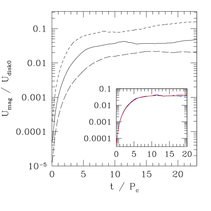
FIG. 13.: Evolution of $U_{\rm mag}$ in unit of initial internal energy of $U_{\rm disk0}$ for $R_{B}=1.3\times 10^{-5}$ (long-dashed curve), $5\times 10^{-5}$ (solid curve), and $2\times 10^{-4}$ (dashed curve). In the smaller panel, we display evolution of $U_{\rm mag}/U_{\rm disk0}$ for $R_{B}=5\times 10^{-5}$ with three levels of grid resolutions with sizes (301, 301) (solid curve), (241, 241) (dashed curve), and (201, 201) (long-dashed curve). Three curves approximately agree.

Simulations are performed for various values of $A$ which is chosen so that the magnetic pressure is initially much smaller than the gas pressure. In the following we specify the model in terms of the initial ratio of the energy of magnetic fields to the internal energy of the disk (hereafter $R_{B}$) instead of $A$. Here, the energy of magnetic fields and the internal energy of the disk is simply defined by

$$U_{\rm mag}\equiv\int_{\rm disk}b^{2}d^{3}x,$$ (149)

$$U_{\rm disk}\equiv\int_{\rm disk}\rho_{*}\varepsilon d^{3}x,$$ (150)

and thus, $R_{B}\equiv U_{\rm mag}/U_{\rm disk}$ at $t=0$. We note that the precise definition of the magnetic energy is unknown in general relativity, but the present definition is likely to give a guideline for the magnitude within an error of a factor of $\sim 2$–3.

In Fig. 13, we show the evolution of $U_{\rm mag}$ for three values of $R_{B}$. Here, the magnetic energy is plotted in units of the initial value of $U_{\rm disk}$ (hereafter $U_{\rm disk0}$) which is about $1.8\times 10^{-4}M_{\rm disk}$. It is found that $U_{\rm mag}$ grows monotonically until the growth is saturated irrespective of the value of $R_{B}$. The growth rate is in proportional to $R_{B}^{1/2}$ in the early phase before the saturation is reached. This indicates that differential rotation winds up the magnetic field lines for amplifying the field strength [12, 13]. After the saturation occurs, $U_{\rm mag}/U_{\rm disk0}$ relaxes to $\sim 0.02$–0.2. These values indicate that the magnetic $\beta$ parameter often referred in [21] is of order $\sim 10$. These relaxed values are in good agreement with previous results obtained in the simulation with a fixed background [21]. The magnetic energy reached after the saturation depends on $R_{B}$, indicating that not only the winding-up of the field lines but also other mechanisms (which may be MRI or other instabilities associated with the magnetic fields) are likely to determine the final value.

To check that the growth of the magnetic fields occurs irrespective of grid resolution, we performed additional simulations for $R_{B}=5\times 10^{-5}$ with grid sizes of (241, 241) and (201, 201) without changing the location of the outer boundaries. In the small panel of Fig. 13, evolution of the magnetic energy for these cases as well as for (301, 301) grid size is displayed. It is shown that the growth rate depends very weakly on the grid resolution. This confirms that our simulation can follow the winding-up of the magnetic field lines well. On the other hand, it should be mentioned that the fastest growing mode of the MRI cannot be resolved in the present computational setting since the characteristic wavelength for this mode $\sim 2\pi v_{A}/\Omega$, where $v_{A}$ denotes the characteristic Alfvén speed, is approximately as small as the grid size (for $R_{B}=5\times 10^{-5}$, $2\pi v_{A}/\Omega\approx\Delta x$) in the current setting. To resolve the fastest growing mode, the grid size should be at least one tenth of the present one. Performing such a simulation of high resolution is beyond scope of this paper and an issue for the next step.

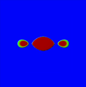
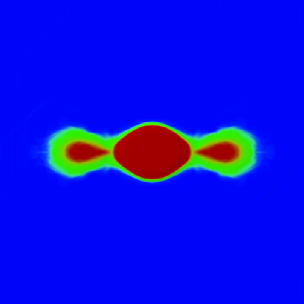
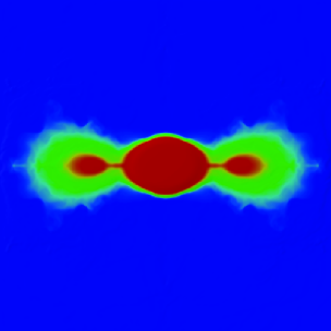
FIG. 14.: Snapshots of the density profile of a neutron and a disk in $x-z$ plane at $t=0$, 9.78, and 19.40 ms for $R_{B}=2\times 10^{-4}$. For $\rho>10^{10}~{}{\rm g/cm^{3}}$, the density is denoted by the same color (red), and for $10^{10}~{}{\rm g/cm^{3}}\geq\rho\geq 10^{7}~{}{\rm g/cm^{3}}$, the color is changed (from red to green).

FIG. 15.: Evolution of $M_{\rm disk}$ and $J_{\rm disk}$ for $R_{B}=0$ (dotted curves), $1.3\times 10^{-5}$ (long-dashed curves), $5\times 10^{-5}$ (solid curves), and $2\times 10^{-4}$ (dashed curves).

In Fig. 14, snapshots of the density profile of disks are displayed for which $R_{B}=2\times 10^{-4}$. It shows that with the growth of magnetic fields due to winding-up of the field lines, a wind is induced to blow the matter in the outer part of the disk off. Also, the matter in the inner part of the disk gradually falls into the neutron star because of the angular momentum transport by the magnetic fields from the inner to the outer parts (see Fig. 15). After the nonlinear development of the turbulence, the disk settles down to a quasi stationary state. As explained in [64, 21], this is probably due to the imposition of axial symmetry which precludes the development of the azimuthal unstable modes. Also, in the present numerical simulation, MRI which could induce turbulence is not well resolved. This may be also a reason.

In Fig. 15, we show the evolution of mass and angular momentum of the disk. It shows that after the saturation of the nonlinear growth of the magnetic fields, these quantities decrease. Decrease rates of the mass and angular momentum take maximum values soon after the growth of the magnetic pressure is saturated (e.g., at $t\approx 5P_{c}$ for $R_{B}=2\times 10^{-4}$; cf. the dashed curves). Then, the mass and angular momentum relax to approximately constants (cf. the dashed curves). This indicates that the disk settles down to a quasistationary state. An interesting feature is that $J_{\rm disk}$ is approximately proportional to $M_{\rm disk}$ throughout the evolution. This is reasonable because the specific angular momentum $j$ is constant in the disk at $t=0$, and approximately so is the matter fallen to the neutron star as long as the magnetic pressure is much smaller than the gas pressure. However, in the case of $R_{B}=2\times 10^{-4}$, at $t\sim 20P_{c}$ for which growth of the magnetic field has already saturated enough, $J_{\rm disk}/M_{\rm disk}$ slightly deviates from the initial value. This indicates that angular momentum is transported by the effect of magnetic fields.

We also performed a simulation for a toroidal magnetic field $B^{\varphi}$. For $B^{\varphi}$, we gave

$$B^{\varphi}=\Big{\{}\begin{array}[]{ll}C(\rho-\rho_{0})z/(z+z_{0})&{\rm for}~{}\rho\geq\rho_{0},\\ 0&{\rm for}~{}\rho<\rho_{0},\end{array}$$ (153)

where $\rho_{0}=0.3\rho_{\rm max:disk}$ and $z_{0}$ is a constant much smaller than the scale hight of the disk. We note that $B^{\varphi}$ has to be zero in the equatorial plane because we impose a reflection symmetry for the matter field with respect to this plane. In this simulation, magnetic energy decreases monotonically due to a small expansion of the disk induced by the magnetic pressure. In this case, no instability sets in. This is a natural consequence since the field lines are parallel to the rotational motion, and hence, they are not wound by the differential rotation. Obviously, the assumption of the axial symmetry prohibits deformation of the magnetic field lines and plays a crucial role for stabilization. If a nonaxisymmetric simulation is performed, MRI could set in [64, 65, 23].

VII Summary and discussion

In this paper, we describe our new implementation for ideal GRMHD simulations. In this implementation, Einstein’s evolution equations are evolved by a latest version of BSSN formalism, the MHD equations by a HRC scheme, and the induction equation by a constraint transport method. We performed a number of simulations for standard test problems in relativistic MHD including special relativistic magnetized shocks, general relativistic magnetized Bondi flow in the stationary spacetime, and fully general relativistic simulation for a self-gravitating system composed of a neutron star and a disk. Our implementation yields accurate and convergent results for all these test problems. In addition, we performed simulations for a magnetized accretion disk around a neutron star in full general relativity. It is shown that magnetic fields in the differentially rotating disk are wound, and as a result, the magnetic field strength increases monotonically until a saturation is achieved. This illustrates that our implementation can be applied for investigation of growth of magnetic fields in self-gravitating systems.

In the future, we will perform a wide variety of simulations including magnetized stellar core collapse, MRI for self-gravitating neutron stars and disks, magnetic braking of differentially rotating neutron stars, and merger of binary magnetized neutron stars. Currently, we consider that the primary target is stellar core collapse of a strongly magnetized star to a black hole and a neutron star which could be a central engine of gamma-ray bursts. Recently, simulations aiming at clarifying these high energy phenomena have been performed [66, 67]. In such simulations, however, one neglects self-gravity and also assumes the configuration of the disks around the central compact object and magnetic fields without physical reasons. On the other hand, Newtonian MHD simulations including self-gravity consistently have recently performed in [68]. However, stellar core collapse to a black hole and gamma-ray bursts are relativistic phenomena. For a self consistent study, it is obviously necessary to perform a general relativistic simulation from the onset of stellar core collapse throughout formation of a neutron star or a black hole with surrounding disks. Subsequent phenomena such as ejection of jets and onset of MRI of disks should be investigated using the output of the collapse simulation. In previous papers [26, 9], we performed fully general relativistic simulations of stellar core collapse to formation of a neutron star and a black hole in the absence of magnetic fields. As an extension of the previous work, simulation for stellar core collapse with a strongly magnetized massive star should be a natural next target.

It is also important and interesting to clarify how MRI sets in and how long the time scale for the angular momentum transport after the onset of the MRI is in differentially rotating neutron stars. Recent numerical simulations for merger of binary neutron stars in full general relativity [6, 7] have clarified that if total mass of the system is smaller than a critical value, the outcome after the merger will be a hypermassive neutron star for which the self-gravity is supported by strong centrifugal force generated by rapid and differential rotation. Furthermore, the latest simulations have clarified that the hypermassive neutron star is likely to have an ellipsoidal shape with a large ellipticity [7], implying that it can be a strong emitter of high-frequency gravitational waves which may be detected by advanced laser interferometric gravitational wave detectors [69]. In our estimation of amplitude of gravitational waves [69], we assume that there is no magnetic field in the neutron stars. However, the neutron stars in nature are magnetized, and hence, the hypermassive neutron stars should also be. If the differential rotation of the hypermassive neutron stars amplifies the seed magnetic field via winding-up of magnetic fields or MRI very rapidly, the angular momentum may be redistributed and hence the structure of the hypermassive neutron stars may be significantly changed. In [7], we evaluate the emission time scale of gravitational waves for the hypermassive neutron stars is typically $\sim 50$–$100$ ms for the mass $M\sim 2.4$–$2.7M_{\odot}$ assuming the absence of the magnetic effects. Here, the time scale of $\sim 50$–$100$ ms is an approximate dissipation time scale of angular momentum via gravitational radiation, and hence in this case, after $\sim 50$–$100$ ms, the hypermassive neutron stars collapse to a black hole because the centrifugal force is weaken. Thus, it is interesting to ask if the dissipation and/or transport time scale of angular momentum by magnetic fields is shorter than $\sim 50$–$100$ ms so that they can turn on before collapsing to a black hole. Rotational periods of the hypermassive neutron stars are 0.5–1 ms. Thus, if the magnetic fields grow in the dynamical time scale associated with the rotational motion via MRI, the amplitude and frequency of gravitational waves may be significantly affected. According to a theory of MRI [30], the wavelength of the fastest growing mode is $\sim 10(B/10^{12}~{}{\rm gauss})(\rho/10^{15}~{}{\rm g/cm^{3}})^{-1/2}(P/1~{}{\rm ms})$ cm where $B$, $\rho$, and $P$ denotes a typical magnetic field strength, density, and rotational period, respectively. This indicates that a turbulence composed of small eddies (for which the typical scale is much smaller than the stellar radius) will set in. Subsequently, it will contribute to a secular angular momentum transport for which the time scale is likely to be longer than the growth time scale of MRI $\sim$ a few ms although it is not clear if it is longer than $\sim 100$ ms. On the other hand, if the transport time scale is not as short as $\sim 100$ ms, other effects associated with magnetic fields will not affect the evolution of the hypermassive neutron stars. Indeed, Ref. [12] indicates that the typical time scale associated with magnetic braking (winding-up of magnetic field lines) depends on the initial strength of the magnetic fields, and it is much longer than the dynamical time scale as $\sim 100~{}(10^{12}~{}{\rm gauss}/B)$ s. In this case, the hypermassive neutron stars can be strong emitters of gravitational waves as indicated in [69]. As is clear from this discussion, it is important to clarify the growth time scale of magnetic fields in differentially rotating neutron stars. This is also the subject in our subsequent papers [63].

- [1] M. Shibata, Phys. Rev. D 60, 104052 (1999): M. Shibata and K. Uryū, Phys. Rev. D 61, 064001 (2000).
- [2] J. A. Font et al., Phys. Rev. D 65, 084024 (2002).
- [3] M. D. Duez, P. Marronetti, T. W. Baumgarte, and S. L. Shapiro, Phys. Rev. D 67, 024004 (2003): M. D. Duez, Y.-T. Liu, S. L. Shapiro, and B. C. Stephens, Phys. Rev. D 69, 104030 (2004).
- [4] M. Miller, P. Gressman, and W.-M. Suen, Phys. Rev. D 69, 064026 (2004).
- [5] L. Baiotti, I. Hawke, P. J. Montero, F. Löffler, L. Rezzolla, N. Stergioulas, J. A. Font, and E. Seidel, Phys. Rev. D 71, 024035 (2005): L. Baiotti, I. Hawke, L. Rezzolla, and E. Schnetter, Phys. Rev. Lett. 94, 131101 (2005).
- [6] M. Shibata, K. Taniguchi, and K. Uryū, Phys. Rev. D 68, 084020 (2003).
- [7] M. Shibata, K. Taniguchi, and K. Uryū, Phys. Rev. D 71, 084021 (2005).
- [8] M. Shibata and Y. Sekiguchi, Phys. Rev. D 71, 024014 (2005).
- [9] Y. Sekiguchi and M. Shibata, Phys. Rev. D 71, 084013 (2005).
- [10] M. D. Duez, Y. T. Liu, S. L. Shapiro, and B. C. Stephens, submitted to PRD.
- [11] S. Akiyama, J. C. Wheeler, D. L. Meier, and I. Lichtenstadt, Astrophys. J. 584, 954 (2003).
- [12] T. W. Baumgarte, S. L. Shapiro, and M. Shibata, Astrophys. J. Lett. 528, L29 (2000).
- [13] S. L. Shapiro, Astrophys. J. 544, 397 (2000): J. N. Cook, S. L. Shapiro, and B. C. Stephens, Astrophys. J. 599, 1272 (2003): Y.-T. Liu and S. L. Shapiro, Phys. Rev. D 69, 044009 (2004).
- [14] T. Zwerger and E. Müller, Astron. Astrophys. 320, 209 (1997).
- [15] H. Dimmelmeier, J. A. Font, and E. Müller, Astron. Astrophys. 393, 523 (2002).
- [16] C. D. Ott, A. Burrows, E. Livne, and R. Walder, Astrophys. J. 600, 834 (2004).
- [17] S. Koide, K. Shibata, and T. Kudoh, Astrophys. J. 522, 727 (1999).
- [18] M. Yokosawa, Publ. Astron. Soc. Japan, 45, 207 (1993).
- [19] S. S. Komissarov, Mon. Not. R. astr. Soc. 350, 1431 (2004).
- [20] C. F. Gammie, J. C. McKinney, and G. Tóth, Astrophys. J. 589, 444 (2003).
- [21] J.-P. De Villiers and J. F. Hawley, Astrophys. J. 589, 458 (2003).
- [22] J. C. McKinney and C. F. Gammie, Astrophys. J. 611, 977 (2004).
- [23] J.-P. De Villiers, J. F. Hawley, and J. H. Krolik, Astrophys. J. 599, 1238 (2003). S. Hirose, J. H. Krolik, J.-P. De Villiers, and J. F. Hawley, Astrophys. J. 606, 1083 (2004): J. H. Krolik, J. F. Hawley, and S. Hirose, Astrophys. J. 622, 1008 (2005).
- [24] M. Aloy, private communication.
- [25] J. R. Wilson, Ann. New York Acad. Sci. 262, 123 (1975).
- [26] M. Shibata and Y. Sekiguchi, Phys. Rev. D 69, 084024 (2004).
- [27] P. Cerda-Duran, G. Faye, H. Dimmelmeier, J. A. Font, J. M. Ibánez, E. Müller, and G. Schäfer, astro-ph/0412611.
- [28] T. Nakamura, K. Oohara, and Y. Kojima, Prog. Theor. Phys. Suppl. 90, 1 (1987) (see Sec. IV of this paper).
- [29] L. Antón, O. Zanotti, J. A. Miralles, J. M. Martí, J. M. Ibánez, J. A. Font, and J. A. Pons, astro-ph/0506063.
- [30] S. A. Balbus and J. F. Hawley, Astrophys. J. 376, 214 (1991): Rev. Mod. Phys. 70, 1 (1998).
- [31] C. W. Misner, K. S. Thorne, and J. A. Wheeler, Gravitation (W. H. Freeman and Company, New York, 1973).
- [32] M. Alcubierre, S. Brandt, B. Brügmann, D. Holz, E. Seidel, R. Takahashi, and J. Thornburg, Int. J. Mod. Phys. D 10, 273 (2001).
- [33] M. Shibata, Prog. Theor. Phys. 104, 325 (2000).
- [34] M. Shibata, Phys. Rev. D 67, 024033 (2003).
- [35] M. Shibata and T. Nakamura, Phys. Rev. D 52, 5428 (1995): T. W. Baumgarte and S. L. Shapiro, Phys. Rev. D 59, 024007 (1999).
- [36] M. Shibata and K. Uryū, Prog. Theor. Phys. 107, 265 (2002).
- [37] M. Shibata, Astrophys. J. 595, 992 (2003).
- [38] J. M. Martí and E. Müller, Living Rev. Relativity 6, 7 (2003).
- [39] S. S. Komissarov, Mon. Not. R. astr. Soc. 303, 343 (1999): See also correction to this paper, astro-ph/0209213.
- [40] D. Balsara, Astrophys. J. Suppl. 132, 83 (2001).
- [41] L. Del Zanna, N. Bucciantiti, and P. Londrillo, Astron. Astrophys. 400, 397 (2003).
- [42] A. Kurganov and E. Tadmor, J. Comput. Phys. 160, 214 (2000).
- [43] A. Lucas-Serrano, J. A. Font, J. M. Ibánez, and J. M. Martí, Astron. Astrophys. 428, 703 (2004).
- [44] A. Harten, P. D. Lax, and B. J. van Leer, SIAM Rev. 25, 35 (1983).
- [45] L. Del Zanna and N. Bicciantini, Astron. Astrophys. 390, 1177 (2002): P. Annios and P. C. Fragile, Astrophys. J. Suppl. 144, 243 (2003).
- [46] A. M. Anile, Relativistic Fluids and Magneto-Fluids (Cambridge University Press, Cambridge, 1989).
- [47] F. Banyuls, J. A. Font, J.-Ma. Ibáñez, J. M. Marti, and J. A. Miralles, Astrophys. J. 476, 221 (1997).
- [48] J. A. Font, Living Rev. Relativity 6, 4 (2003).
- [49] C. R. Evans and J. F. Hawley, Astrophys. J. 332, 659 (1988).
- [50] G. Tóth, J. Comput. Phys. 161, 605 (2000).
- [51] M. Bocquet, S. Bonazzola, E. Gourgoulhon, and J. Novak, Astron. Astrophys. 301, 757 (1995).
- [52] K. Maeda and K. Oohara, Prog. Thoer. Phys. 68, 567 (1982).
- [53] J. W. York, Jr., in Sources of Gravitational Radiation, ed. L. L. Smarr (Cambridge University Press, 1979), p. 83.
- [54] M. Aloy, private communication.
- [55] J. F. Hawley, L. L. Smarr, and J. R. Wilson, Astrophys. J. 277, 296 (1984).
- [56] R. F. Stark and T. Piran, Comp. Phys. Rep. 5, 221 (1987).
- [57] S. L. Shapiro and S. A. Teukolsky, Black Holes, White Dwarfs, and Neutron Stars, Wiley Interscience (New York, 1983).
- [58] J. R. Wilson and G. J. Mathews, Phys. Rev. Lett. 75, 4161 (1995).
- [59] G. B. Cook, S. L. Shapiro, and S. A. Teukolsky, Phys. Rev. D 53, 5533 (1996).
- [60] N. Stergioulas, Living Reviews in Relativity 6, 3, (2003).
- [61] M. Shibata and J. A. Font, Phys. Rev. D (2005) in submission.
- [62] A. Akmal, V. R. Pandharipande, and D. G. Ravenhall, Phys. Rev. C 58, 1804 (1998): F. Douchin and P. Haensel, Astron. Astrophys. 380, 151 (2001).
- [63] Works in progress in collaboration with M. Duez, Y.-T. Liu, S. L. Shapiro, and B. C. Stephens, in preparation.
- [64] J. F. Hawley, Astrophys. J. 528, 462 (2000): J. F. Hawley and J. H. Krolik, Astrophys. J. 566, 164 (2002).
- [65] M. Machida, M. Hayashi, and R. Matsumoto, Astrophys. J. Lett. 532, L67 (2000).
- [66] A. I. MacFadyen and S. E. Woosley, Astrophys. J. 524, 262 (1999).
- [67] Y. Mizuno, S. Yamada, S. Koide, and K. Shibata, Astrophys. J. 606, 395 (2004); ibid 615, 389 (2004).
- [68] T. Takiwaki, K. Kotake, S. Nagataki, and K. Sato, Astrophys. J. 616, 1086 (2004), and references cited therein.
- [69] M. Shibata, Phys. Rev. Lett. 94, 201101 (2005).