Steps towards a solution of the FS Aurigae puzzle.
I. Multicolour high-speed photometry with ULTRACAM.

Abstract

We present the analysis of high-speed photometric observations of FS Aur taken with the 4.2-m William Herschel Telescope and the high-speed camera ULTRACAM in late 2003. These observations were intended to determine whether there was any evidence of photometric variability with a period in the range 50–100 seconds. The discovery of such variations would help to explain existence, in FS Aur, of the very coherent photometric period of 205.5 min that exceeds the spectroscopic period by 2.4 times. Such a discrepancy in the photometric and spectroscopic periods is an unusual for a low mass binary system that is unambiguously identified as a Cataclysmic Variable. Using various methods, including wavelet-analysis, we found that with exception of the 205.5-minute periodicity, the main characteristic of variability of FS Aur is usual flickering and Quasi-Periodic Oscillations. However, we detected variability with a period of $\sim$101 and/or $\sim$105 sec, seen for a short time every half of the orbital period. These oscillations may be associated with the spin period of the white dwarf, not ruling out the possibility that we are observing a precessing rapidly rotating white dwarf in FS Aur.

1 Introduction

Cataclysmic Variables (CVs) are close interacting binaries that contain a white dwarf accreting material transferred from a companion, usually a late main-sequence star. CVs are very active photometrically, exhibiting variability on time scales from seconds to centuries (see review by Warner 1995). In this paper we concentrate on FS Aurigae, a cataclysmic variable with rather unusual photometric behaviour.

FS Aur was discovered and first classified as a dwarf nova by Hoffmeister (1949). This system varies between approximately V=15$\aas@@fstack{m}$4–16$\aas@@fstack{m}$2 in quiescence and V=14$\aas@@fstack{m}$4 in outburst. Thorstensen et al. (1996) defined the orbital period of 0.0595 days (=85.7 min) from H$\alpha$ spectroscopy and suggested an SU UMa classification based on the short orbital period: “In view of the preponderance of SU UMa stars among the dwarf novae in this period range, we would be surprised if superoutbursts and superhumps were not detected in the future”. However no superoutburst/superhumps have ever been observed in FS Aur. So the SU Uma classification of this star is uncertain.

Table 1: Log of ULTRACAM observations.

Date	UT	Run	Number	Exposure	Filters	Comments
	start - end		of points	(sec)
2003-10-30	00:57:39 - 01:38:00	run021(a)	484	5.01	ugi	Cirrus and poor seeing ($>$3″)
2003-10-30	01:58:28 - 02:36:12	run021(b)	450	5.01	ugi	Cirrus and seeing improving
2003-10-30	02:37:36 - 03:19:45	run023	506	5.01	ugi
2003-10-30	04:06:16 - 04:20:38	run026	157	5.01	ugi	Seeing around 1″. Hit rotator limit
2003-10-30	04:36:58 - 05:39:13	run027(a)	28	5.01	ugi	Cirrus again
2003-10-30	05:45:09 - 05:49:27	run027(b)	727	5.01	ugi	Cirrus and seeing improving
2003-11-03	03:10:50 - 03:40:45	run065	824	2.18	ugr
2003-11-03	03:40:57 - 04:10:07	run066	803	2.18	ugr	Run stopped for zenith blind-spot slew
2003-11-03	04:13:35 - 04:44:08	run067	841	2.18	ugr
2003-11-03	04:44:17 - 05:14:21	run068	828	2.18	ugr
2003-11-03	05:14:29 - 05:44:14	run069	819	2.18	ugr
2003-11-03	05:44:25 - 06:14:34	run070	830	2.18	ugr
2003-11-03	06:15:02 - 06:16:17	run071	35	2.18	ugr	Dome closed due to high humidity

Moreover, recently another more outlandish peculiarity of FS Aur has been discovered. Neustroev (2002) in the first detailed investigation of this system noted, and Tovmassian et al. (2003) confirmed on the base of a large dataset spanning for several years that this system shows a well-defined photometric optical modulations with 205.5 minutes periodicity and the amplitude of 0.24 mag in B, V and R bands. This is in contrast to the spectroscopic period of 85.7 minutes, also confirmed by Neustroev (2002) and Tovmassian et al. (2003).

In addition to FS Aur, there are a few other CVs with a photometric period that exceeds the spectroscopic one. These are GW Lib (Woudt & Warner, 2002), Aqr1 (Woudt, Warner, & Pretorius, 2004) and probably SDSS 1238 (Zharikov et al., 2005). There is no obvious relationship between photometric and spectroscopic periods of these objects. However, due to insufficient observational coverage of the latter objects it is unclear how stable and coherent the photometric modulations are. For example, the 125.4-min modulation in the best known system GW Lib were observed for only two weeks and were not detected in other observations. At the same time, the photometric modulations of FS Aur have been observed to be coherent from ten years of observations (Tovmassian & Zharikov 2004; Neustroev et al., in preparation). On the other hand several high frequency periodic signals were detected in the light curve of GW Lib (van Zyl et al., 2004) and it has been argued that they are ZZ Cet type pulsations of a WD. More observations are needed to determine the similarities and differences of these objects.

The reason for the strange behaviour of FS Aur is not yet clear. Tovmassian et al. (2003) concluded that the “usual” effects explaining photometric period that are longer than spectroscopic, can be effectively ruled out. In particular, it is difficult to directly apply the intermediate polar scenario to the case of FS Aur. There are theoretical restrictions on upper limits of the spin periods of IPs, and 205 min is very unlikely to be the period of rotation of the WD.

Tovmassian et al. (2003) also showed that a possible explanation of this puzzle might be a rapidly rotating magnetic white dwarf in FS Aur freely precessing with a period equal to the observed photometric period. The chance to see this precession period in optical wavelengths would only be when the collimated beam from the magnetically accreting white dwarf, the rotational axes of the white dwarf and the binary orbital plane would have certain angles relative to each other. This could explain the uniqueness of FS Aur and why we observe such periods so rarely.

In order to have the proposed precession period, the rotational white dwarf spin period should be of the order of 50–100 sec, according to existing models (Leins et al., 1992), i.e. the white dwarf in FS Aur could be a fast rotator such as AE Aqr and DQ Her. This hypothesis remains, however, highly debatable until firm evidence of the fast rotating white dwarf in this system is found. We suggest that this phenomenological model can be observationally tested with fast optical photometry. Indeed, if we accept that the photometric variability comes from the free precession of the magnetic white dwarf, or rather reflection of the high energy beam originating at accreting poles from elsewhere in the system, then one can reasonably expect to see variability associated with the rotation period itself. Furthermore we might expect a relationship between the precessional, orbital and rotational periodicity.

In this paper we present the analysis of high-speed photometric observations of FS Aur which were intended to determine whether such fluctuations exist, and we report new interesting features of this system.

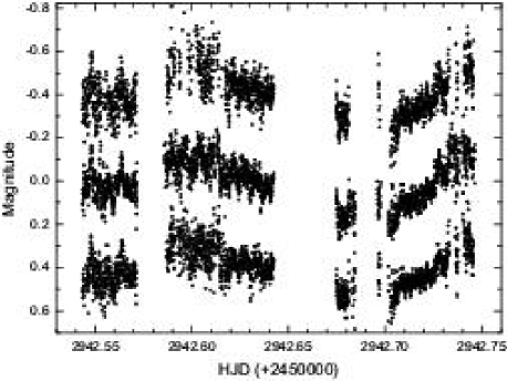
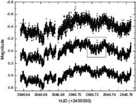
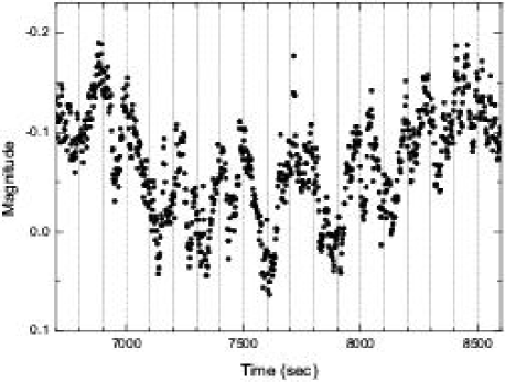
Figure 1: The ULTRACAM light curves of FS Aur, obtained on the nights of 29 October 2003 (upper panel) and 2 November 2003 (middle panel). The data for the each colour band were normalized to its average nightly magnitude, after that a vertical shift of 0.4 mag has been introduced between light curves for display purposes. Upper and medium light curves are for the $u^{\prime}$ and $g^{\prime}$ filters, respectively, and lower curves are for the $i^{\prime}$ filter (first night, upper panel) and $r^{\prime}$ filter (second night, middle panel). Bottom panel shows the marked part of the $g^{\prime}$-band light curve from second night on a larger scale.

2 Observations

FS Aur was observed on the nights of 29 October 2003 and 2 November 2003 using ULTRACAM in Service mode on the 4.2-m William Herschel Telescope (WHT) at the Isaac Newton Group of Telescopes, La Palma. ULTRACAM is an ultra-fast, triple-beam CCD camera designed to provide imaging photometry at high temporal resolution in three different colours simultaneously (for further details see Dhillon & Marsh 2001). Our observations were obtained simultaneously in the SDSS $u^{\prime}$, $g^{\prime}$, and $i^{\prime}$ colour bands on 29 October (hereinafter we call this set of observations as first night), and the SDSS $u^{\prime}$, $g^{\prime}$, and $r^{\prime}$ bands on 2 November (second night). The $u^{\prime}$, $g^{\prime}$, $r^{\prime}$ and $i^{\prime}$ filters have effective wavelengths of 3550 Å, 4750 Å, 6200 Å  and 7650 Å  respectively.

The weather conditions during the first night were not optimal due to cirrus and poor seeing (down to 3″). We removed the poor data from the first dataset, and used the rest for this investigation. During the second night the weather conditions were on the whole good. This, almost evenly sampled dataset, of more than three hours duration has very small gaps. For the first night, we used an exposure time of 5.0 sec; on the second night the exposure time was decreased to 2.18 sec.

A log of the observations is given in Table 1.

Data reduction was carried out using the MIDAS package in conjunction with Fortran code. All extracted images were debiased and flat-fielded in a standard fashion within MIDAS. Unfortunately, we were unable to observe a standard star using ULTRACAM, so the zeropoints for all the filters could not be calculated. However, this will only affect the scale of the light curves, not their shape. The usual and previously used comparison stars C1, C3 and C4 from Misselt (1996) were included in the field of view so that differential photometry could be obtained. We calculated magnitudes of the source with respect to the C1, using aperture photometry. As a check of the photometry and systematics in the reduction and extraction procedures, we also computed magnitudes of the comparison stars C3 and C4. For the second night the differences between nightly averages of the differential magnitudes (C1-C3, C1-C4) were within 0.03 mag for the $g^{\prime}$ and $r^{\prime}$ filters and 0.1 for the $u^{\prime}$ filter. The same differences for the used data of the first night were within 0.05 mag for the $g^{\prime}$ and $i^{\prime}$ filters and 0.1 for the $u^{\prime}$ filter. The appropriate standard deviations of these differences were within 0.015 mag for $g^{\prime}$, $r^{\prime}$ and $i^{\prime}$ and 0.05 for $u^{\prime}$ for both observational nights.

In this paper we also used data from our previous observations taken with the 1.5-m telescope of OAN SPM on JD 2451946, we will refer to this dataset as set-1946. Though this data has a time resolution worse than the ULTRACAM-data ($\sim$20 sec), it covers a longer time span (315 minutes). All details on these observations can be found in Tovmassian et al. (2003).

3 ULTRACAM light curve analysis

3.1 Light Curve Morphology

Fig. 1 shows the ULTRACAM light curves of FS Aur. The most prominent feature is the quasi-sinusoidal shape. These light curves can be easily combined with older photometrical data of FS Aur, confirming the very coherent nature of the periodic signal with the period of $\sim$205.5 minutes covering ten years of observations (Neustroev et al., in preparation). Additionally, both datasets show strong modulations (with an amplitude up to 0.15-0.20 mag) on both medium ($\sim$10 min) and short ($\sim$100 sec) timescales. This variability is evident in all filters. Moreover, all the light curves are very correlated and the modulations in each have almost the same amplitude.

On both nights the mean V magnitude was about 15.7, calculated using the transformation formulae between the UBVRI and SDSS systems of Smith et al. 2002 indicating that FS Aur was definitely in the quiescent state.

In the bottom panel of Fig. 1 we show part of the $g^{\prime}$-band light curve from second night. A period of the order of $\sim$100 s is quite apparent to the eye, but on closer inspection the variability appears to be very complex - the interval between maxima is not constant.

In the following analysis, due to the better quality and more homogeneous nature of the data, we shall use data from the second night and then compare these results with the first night.

3.2 Power Spectra

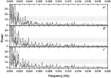
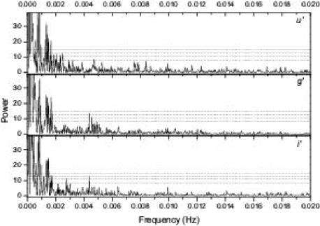
Figure 2: The power spectra of the second (upper) and first (bottom) night’s light curves. The overplotted dashed lines are 50%, 95%, 99% and 99.9% significance levels.

Using the standard Lomb-Scargle power spectrum analysis (Lomb, 1976; Scargle, 1982), we calculated the power spectra on individual nights (Fig. 2, note the high coincidence between the power spectra in the different filters). There are a number of strong peaks in the spectra. In order to understand the significance of these peaks are, we evaluated their significance level using a classical method based on white noise (Press et al., 1992). However we note that the presence of red-noise will alter the significance levels compared to Gaussian noise models, see discussion in Section 5.1.

All the power spectra are dominated by the fundamental frequency of $1/P_{phot}$ ($8.1\times 10^{-5}$ Hz) and its harmonics. However there also are the other strong peaks with a high significance level. But after comparing, one can see that the power spectra from the different nights are significantly different. Almost all the strongest peaks of one night are completely absent in the other and vice versa, and only few from them have weak counterparts ($\sim$1.50 mHz and 3.86 mHz). In the frequency range of interest ($\sim$10–20 mHz) one can see, in both night’s power spectra, some relatively strong peaks around 10 mHz. However, their frequencies do not coincide exactly.

In order to investigate a transition and a mutation of the peaks, we split up each light curve into four sets of almost equal length and analyzed all independent sets individually. None of the calculated spectra is similar to any other. The above mentioned peaks appear/disappear very quickly, on the subsequent data sets, so their transition time is very short. The reason for this is probably simple flickering seen in many CVs.

3.3 Sliding periodograms and Wavelet analysis

In order to study how stable the peaks in the power spectra are, the common practice is to split the complete time series into a few separate sets and analyse them individually. Frequently unjustified significance is given to the lack of some peaks in some subsets with these peaks being eliminated from further analysis. However it may be important to retrace changes of these peaks with time. For this we can calculate power spectra for complete time-series as well as power spectra from a sliding window moved across the full time series with a width of $\Delta$T.

Such an approach can be described, using a short time Fourier transform or windowed Fourier transform, Gabor (1946):

$$GT(\nu,t_{0},\sigma)=\int\limits_{-\infty}^{\infty}{f(t)e^{-\frac{{(t-t_{0})^{2}}}{{\sigma^{2}}}}e^{-i2\pi\nu t}dt}$$ (1)

where constant $\sigma$ determines the effective width of the Gabor transform window, and $t_{0}$ is the centre of the latter. Moving the centre of the window along the time series $f(t)$, allows us to obtain “snapshots” of the time-frequency behaviour of $f(t)$. The effective width $\sigma$ determines length of an interval $\Delta$T which gives the main contribution to value of integral (1). Here it is important to note that $\Delta$T is a measure of the time resolution while the linewidth $\Delta\nu$ determines a measure of the frequency resolution.

Since $\Delta\nu$ and $\Delta$T are inversely related, there is a problem of the choice of window width. Too broad a window can provide a reasonable representation of low-frequency components of the time series, but its width will be redundant for high frequency harmonics, as all irregularities in high-frequency area of a spectrum will smooth out. On the contrary, a narrow window will enable us to study variations in time of the high-frequency features, but it will not be adequate for low-frequency harmonics. However, having long enough time series with high time resolution a compromise can be reached.

On the other side, wavelet analysis (Mallat, 1987) offers an alternative to Fourier based time-series analysis and it is particularly useful when spectral components are time dependent. The wavelet transform represents one-dimensional signals as a function of both time and frequency and is similar in this regard to a windowed Fourier transform, but, with one major difference, namely the window function depends on frequency so that for low frequencies the window became wider, and for high frequencies - narrower. Consequently the wavelet transform effectively allows for a multi-scale analysis of a time series.

Standard wavelet methods require time series to be evenly spaced. Foster (1996) developed the weighted wavelet Z-transform (WWZ) that appears to be an effective method of the analysis of unevenly sampled data. The idea behind this technique is basically the same as that behind the Lomb-Scargle periodogram: wavelet trial functions are extended and corrected by a rescale procedure to satisfy the admissibility condition on the uneven grid of times of a data record. In this case the wavelet transform becomes a projection onto trial functions that resemble the shape of the data record (see also an analysis of this method by Haubold 1997).

In spite of the fact that the WWZ method seems to have an advantage over a Fourier transform in our analysis we start with the latter and then go onto the Wavelet anaysis. There are two reasons for this. Firstly, many nuances of the WWZ are unknown. For example, the decay constant $c$ in this method defines the width of the wavelet “window”. Smaller values of $c$ will produce wider windows. Using small values of $c$ will result in improved frequency resolution of variations, but will smear out temporal variations. Conversely, large values of $c$ will improve the temporal resolution, but will generate larger uncertainties in peak frequency. So criteria for choosing $c$ are not quite clear. Secondly, we need a direct comparison of these new calculations with previously obtained Lomb-Scargle periodograms.

3.3.1 Sliding periodograms

To obtain the sliding periodogram (i.e. the full set of the power spectra calculated with the window moving along all the time series) we calculate the Lomb-Scargle periodogram in the selected window moving along the time series, rather than compute integral (1). Formally for the case of evenly spaced data $f(t_{i}),i=1,...,N$ it can be described as

$$SP(\nu,T_{i},N_{W})=LSP(\nu,i,i+N_{W}-1)$$ (2)

$$i=1\rightarrow N-N_{W}+1$$

where $N_{W}$ is number of the points in the window, $LSP$ is the Lomb-Scargle periodogram, calculated in the window formed from a data point $i$ up to a data point $i+N_{W}-1$, and $T_{i}$ is the effective time of the window centre

$$T_{i}\equiv\frac{1}{{N_{W}}}\sum\limits_{j=i}^{i+N_{W}-1}{f(t_{j})},\qquad i=1\rightarrow N-N_{W}+1$$ (3)

If necessary equation (2) can be easily extended for the case of unevenly sampled data.

This approach has obvious advantages over computing the integral (1). Namely, calculated periodograms in the every window are the usual Lomb-Scargle periodograms and can be directly compared with periodograms obtained on the complete sequence of data. We can also easily determine the reliability of any features in a periodogram. Such approach is much faster.

Before calculating the sliding periodogram for the second night we have preprocessed the data. In order to obtain nearly evenly sampled values of $T_{i}$, due to some small gaps in the time series, these were filled by the mean value of the data. We have also experimented with different numbers of points $N_{W}$ in the window, which defines the tradeoff between time resolution and frequency resolution, and settled on $N_{W}$=500 as a good compromise. Such window has a time span of about 1000 sec. And finally, the time series was detrended by subtraction of the smoothed dataset formed from the original by averaging 300 adjacent data points. This was valid as the periodogram calculated for the detrended dataset, shows the same features with almost the same strength. The exceptions were the components of lowest frequency, which could not be investigated by the proposed method.

We have also obtained a sliding periodogram for the first night. Since these data have several large gaps we have split the data into three continuous sets and analyzed them separately, then combined all the results into one the sliding periodogram. Moreover, in order to obtain the same frequency resolution we decreased the numbers of points in the window $N_{W}$ to 200.

The sliding periodograms (or slidograms) as grey-scale images are displayed in the left column of Fig. 3. As the slidograms are based on the usual Lamb-Scargle periodograms we can easily calculate the significance levels, marked in the images by isophots. Immediately one can see that some features show substantial frequency variations with time.

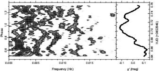
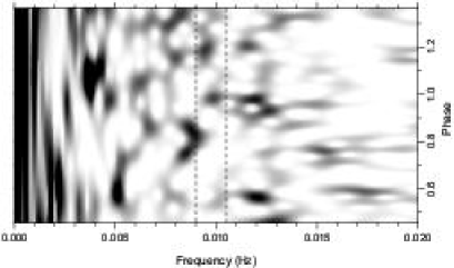
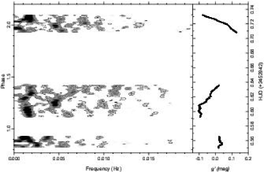
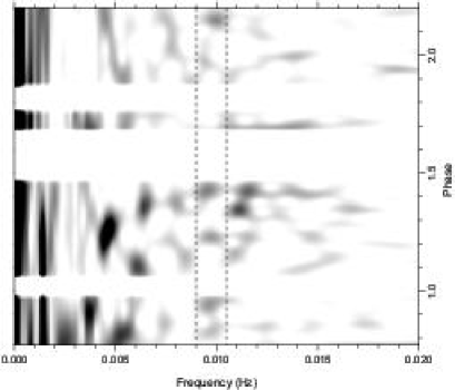
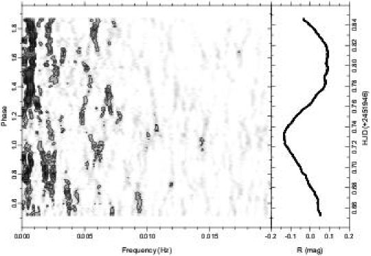
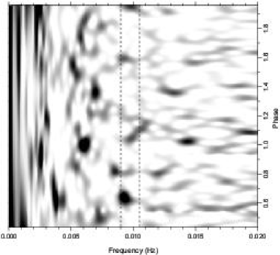
Figure 3: The sliding periodograms (slidograms) and the WWZ wavelet transforms (scalograms) for the second night (upper row), first night (middle row) and set 1946 (bottom row), shown as grey-scale images. The slidograms are displayed in the left panel of the graphics in the left column, while the right panels of these graphics show the light curve. The scalograms are displayed in the right column. Isophots in the sliding periodograms display the significance levels: 90%, 99% and 99.9% for the second night and 50%, 90%, 99% and 99.9% for the first night and the set 1946. Dashed vertical lines in the scalograms images denote the frequency range with regular appearance of “the drops” (see text for explanation). Phases of photometric period are calculated according to the ephemeris for times of maxima: HJD_max=$2450492.3006+0.14270785E+5.5\times 10^{-10}E^{2}$ (Neustroev et al., in preparation).

3.3.2 Wavelet analysis

The WWZ method (Foster, 1996) does not require time series to be evenly spaced and without gaps, so we can work with the original data. On the other hand, in order to find a compromise between the frequency and temporal resolution an optimal value of the decay constant $c$ has to be chosen (in fact, $c$ is playing the role of a parameter). After some experiments we settled on $c$=0.001, although this value is not optimal for all frequencies.

Our results are shown in the right column of Fig. 3. There is a strong simularity between the slidograms and the wavelet transforms (scalograms) but the latter have improving frequency resolution in the frequency range of about 0.003 – 0.013 Hz. At the same time, the lowest frequency part of the scalograms is very smoothed along time axis (i.e. has insufficient temporal resolution). The highest frequency part, on the contrary, is smoothed along the frequency axis.

4 Interpretation

The main distinctive feature of the power spectra of FS Aur is the presence of a number of strong peaks. These however, are not seen on both nights of observations (Fig. 2). On the other hand, the multipeaked comb-like structure of the periodograms testifies, most likely, to the existence and interrelation of these peaks but not to their stability. Analysis of the spectra of separate subsets indicates that these periodic processes are of short duration.

On close inspection one can see that most of the peaks in the power spectra are grouped into a few groups in the following frequency ranges: 0.8–1.1 mHz, 1.3–1.8 mHz, 2–4 mHz, 4–6 mHz, and maybe a few others with higher frequencies. Such grouping are justified from a consideration of the slidograms and the scalograms.

We would like to note the most prominent features in these:

1. There are a number of lines directed along the time axis, and practically no lines directed perpendicularly of this axis (such lines in the scalograms can be explained by the insufficient frequency resolution at the highest frequencies).

2. There are no strictly vertical lines existing continuously in all time ranges.

3. Nevertheless there are a few very strong short segments of nearly vertical lines. In the scalograms they sometimes look like “drops”. Some of them are located along the time axis. It explains why the power spectra of some subsets show the very strong peaks that are missing in the other subsets.

4. Frequently one can see splitting, or on the contrary – confluence, of lines. In some areas of the scalograms this looks like a honeycomb structure.

5. There are long and short sine-like lines with variable intensities and frequencies. This feature explains the grouping of the peaks that was marked earlier.

Some of these features (especially the last) were unexpected, so we conducted a similar analysis of the light curves of several comparison stars and found no similar peculiarities. To confirm these features we also analyzed the light curve of set-1946 and obtained basically the same results (see bottom panel of Fig. 3).

Producing slidograms and scalograms from known test time-series (see Appendix A) the above numbered features at our time-series can be interpreted as follows:

1. Orientation of the lines in the slidograms and the scalograms mainly along the time axis indicates the existence, in the light curve of FS Aur, of sine-like components. Moreover, values of all the periods obtained in the Lomb-Scargle periodograms, are verified in the scalograms, showing that these periodograms have registered quasiperiodic signals which arose and disappeared in a random way.

2. Absence of the strictly vertical lines in all the scalograms testifies to absence of strictly periodic (coherent) signal in the investigated frequency range.

3. However, strong pieces of nearly vertical lines seen at some frequencies ($\sim$1.5 mHz, $\sim$3.9 mHz, probably at $\sim$13 mHz), can be seen in all the scalograms. Due to observed significant variability of their frequency and amplitude with time, we are not ready to call these features strictly periodic. In fact, their behaviour resembles Autoregressive processes (Fig. 10) and most likely these are some kind of classical QPOs. But, we would like to pay particular attention to the so-called “drops” and short lines seen also in all sets of observations at $\sim$9.5–10 mHz. These drops are confined to a narrower range of frequencies, and seem to be located along the time axis at intervals of $\sim$0.2 of the photometric period, that corresponds to nearly half of the orbital period. We have integrated the WWZ in the frequency range of 9–10.5 mHz, and transformed the time of observations to the orbital periods, with arbitrary phase shift for every dataset (Fig. 4). One can see the WWZ maxima are really located through every half of the orbital period, with a few exceptions in the first night and set 1946. These exceptions, as well as scattering of the drops around the mean frequency, can be easily explained by an influence of noise (see an appearance of the test function $F_{5}$ in the slidogram in our last test in Appendix A). This means that we probably see the recurrent appearance of modulations, seen every half of the orbital period.

4. The honeycomb structure of the scalogram is a corollary of strictly stochastic processes similar to white noise (Fig. 10). The splitting and confluence of the strong lines can arise also due to the Autoregressive processes.

5. Sine-like lines can arise from strictly periodic processes similar to an frequency modulation, and from Autoregressive processes. However, in the latter case it is difficult to obtain a sensible frequency deviation and regular sinusoids. In this context a sinusoid at $\sim$5–6 mHz is apparent. This can be seen in all the sliding periodograms and scalograms, though not during all time of the observations. It is interesting to note, that in the second night and possibly in set-1946 this sinusoid is accompanied by another with higher frequency, where their maximal strength is reached in an antiphase.

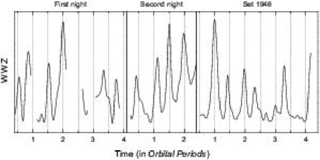
Figure 4: Time dependence of the WWZ integrated in the frequency range of 9–10.5 mHz. Time of observations has been transformed to the orbital periods with arbitrary phase shift for display purpose.

5 Discussion

With the exception of the 205.5-minute periodicity, the main characteristic of variability of FS Aur is the usual CV flickering plus QPOs. The two following features deserve special attention: (i) the frequency-modulated oscillations at $\sim$5-6 mHz (150-200 sec); and (ii) the recurrent appearance of modulations with period of $\sim$100 sec. The former is simply extremely unusual and to the best of our knowledge has never been observed before, whereas the second could be the spin period of the white dwarf or at least connected to it.

5.1 Significance tests

At low frequencies the usual statistical significance tests, based on the assumption of Gaussian white noise, should not be applied to determination of significance levels of peaks in Lomb-Scargle periodograms. Red-noise more adequately to describes CV flickering. In contrast to white noise, the power spectra of red-noise shows a continuous decrease of spectral amplitude with increasing frequency, and frequently shows very strong peaks.

We have investigated the significance of the observed power-series using two methods. Firstly, we have calculated confidence limits for our observed power spectra and shown which peaks are really ”significant”. However it is well known that some strictly periodic functions can produce quite weak peaks in power spectrum, even without any noise (see examples in Appendix A). So, in the second test, we calculated a set of artificial scalograms and compared them with the observed ones in order to understand if red noise could reproduce the observed features.

We calculated the confidence limits using a well developed approach from the Geosciences (Schulz & Mudelsee 2002). Briefly this procedure can be described as follows. Firstly the observed time-series were approximated by Autoregressive (AR) processes of different order, in order to determine which AR model reproduces the power spectra slope. These derived optimal parameters are then used for the calculation of a large set of simulated time-series using the observed times. These artificial time-series can then be used to estimate the significance levels of the Lomb-Scargle periodograms (for more details see also paper of Hakala et al. (2004) for application of this method to astronomical data analysis).

Estimation of the AR parameters from the time-series is a relatively straightforward procedure, but only for evenly sampled data. For unevenly spaced data this technique would require some sort of interpolation. Unfortunately, this procedure may result in a significant bias (Schulz & Stattegger, 1997). Schulz & Mudelsee (2002) presented an algorithm that estimates the AR parameters directly from unevenly spaced series, but only for AR process of the first order. This is probably insufficient to describe our time-series. Fortunately, our second night’s time-series are almost evenly spaced and contain only short gaps, and consequently should not affect the power spectra continuum distribution.

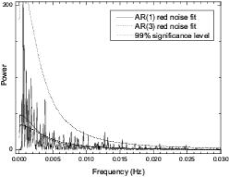
Figure 5: The $g^{\prime}$-band power spectrum of the second night with AR(1) and AR(3) red noise models, and the 99% significance level based on AR(1).

Because the light curve of FS Aur includes a periodic component with the period of $\sim 205.5$ min, the time-series has been pre-whitened before the subsequent analysis. Fitting AR processes to the time-series of the second night shows that already a third-order AR model is more than enough to reproduce the observed power spectrum slope. However, there is insignificant difference between AR(1) and AR(3) in the high-frequency part of the spectrum, AR(1) is better in the medium-frequencies. So we have decided that a first-order Autoregressive process is sufficient to describe the red-noise flickering in FS Aur. Using this AR(1) model we have calculated the significance levels for the power spectrum of the second night and shown these in Fig. 5. One can see that almost all peaks are below the 99% significance level and can be easily explained by red noise confirming our previous conclusions. At the same time it says nothing about the existence of the frequency-modulated oscillations and 100 sec variability as we did not expect to have strong peaks from them. However, the latter shows a significance level of more than 99%.

In order to investigate more throughly the significance of these results we performed a Monte-Carlo analysis. On the base of earlier obtained AR(1) model we have simulated more than 200 time-series, which were used for calculating the scalograms. We then performed a quick-analysis of every artificial scalogram in the same way as the observed ones. Our purpose was to find structures similar to sinusoids on $\sim$ 5-6 mHz and the recurrent “drops” in all the frequency range up to 20 mHz, not only near to 10 mHz. Worrying about the clarity of experiment we have also repeated this analysis for more than 200 artificial scalograms obtained on the base of AR(3) model.

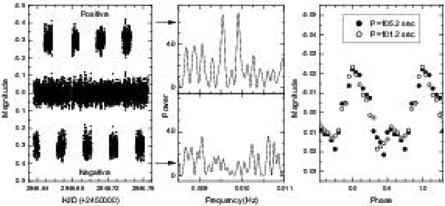
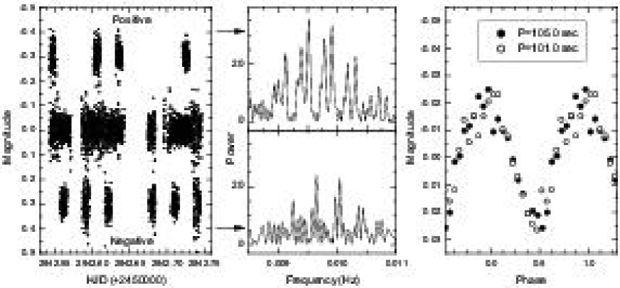
Figure 6: The upper row belongs to the second night’s data, the bottom row to the first night’s data. Left frame: Detrended $g^{\prime}$-band light curve (middle) and the Positive- (upper) and the Negative- (bottom) samples of it (see text for explanation). The samples are displaced by -0.3 and +0.3 mag. Middle frame: Power spectra of the samples. Note that frequencies of the two strongest peaks in the power spectra of the Positive-samples of the both nights completely coincide. Right frame: The mean waveform obtained by folding the Positive-sample on the period of $\sim$101 and $\sim$105 sec.

We found that (i) none of the scalograms showed clear large-amplitude sinusoids; (ii) in almost 500 trials we performed to search for series of periodicities separated by half the orbital period, this was only observed twice in the simulated data in which only three successive periodicities (with periods of $\sim 70$ sec and $\sim 100$ sec) were observed. Whereas in all the real data sets this sequence was observed at least four times (Figs. 3 and 4).

So our conclusion is that both features (the frequency-modulated oscillations and the recurrent appearance of modulations with period of $\sim$100 sec) are real and cannot be readily explained by red-noise.

5.2 100 sec variability

The most persistent peaks of high significance levels are those concentrated around frequencies corresponding to $\sim$0.01 Hz. However, we were unable to find any coherent modulations with periods of 50–100 sec existing continuously in all time ranges, as well as with other periods shorter than tens of minutes. This is disappointing, but probably not very surprising. Even within the suggested hypothesis of the rapidly rotating and precessing magnetic white dwarf one would expect to detect the emission from the accretion poles in high energy range only, and to see only the reprocessed/reflected echo in optical wavelengths. If the high energy beam hits different parts of the disc due to the precession, then magnitude of pulses can be variable or they might disappear altogether during part of the period. Therefore we have reasons to think that detected oscillations with the period of about 100 sec, seen during short time in the slidograms and scalograms every half of the orbital period, can turn out to be the required variability.

Are these real effects or noise? One can see several other series of “drops” located along the time axis of all the scalograms (for example, at $\sim$12–13 mHz). However, in all these cases the time interval between “drops” is variable, and only for 100-second oscillations is this time interval approximately constant and equal to half of the orbital period. Last fact is especially indicative. Any discovered periodic events with the period equal to the orbital one or multiple to it, should be considered very seriously.

In previous subsection we have already shown that there is only a small probability that these 100-seconds events are due to red noise. Additional evidence for their reality come from an assumption that the 100-second oscillations can be detected periodically and only for a short time. Using the detrended time-series of the second night we have prepared two samples, each of them includes about a third of all points. These samples consist of subsets located through each half of the orbital period. The subsets of the first sample are centred on the “drops” in the scalograms (which we will refer to as “the Positive-sample”) while the subsets of the second sample (“the Negative-sample”) are shifted relative to them on a quarter of the orbital period (Fig. 6, upper-left frame). If our assumption is correct then one can expect to see stronger $\sim$100-seconds peak in the power spectrum of the Positive-sample in comparison to the Negative-sample. Our analysis confirms this (Fig. 6, upper-middle frame). The Positive power spectrum shows two strong peaks (at $\sim$9.5 and $\sim$9.9 mHz) completely absent in the Negative spectrum. We have also applied the same approach to the first night’s dataset. Though the spectral window in this case is much more complex, we have obtained exactly the same results (Fig. 6, bottom row). Moreover, frequencies of the two strongest peaks in the power spectra of the Positive-samples of the both nights completely coincide.

On the basis of these data sets we are unable to determine which of these peaks is the real period. Either one of them could be the alias of other. Taking into account the equal strength of the peaks, also both periods could be present in the time-series. Right frames of Fig. 6 show the mean waveforms, obtained by folding the data on these periods (101.0 and 105.0 sec for the first night, and 101.2 and 105.2 sec for the second). All the waveforms are very similar and almost symmetric. The full amplitude is $\sim$0.04 mag.

Our analysis shows that the $\sim$100-seconds oscillations really exist in the light curves of FS Aur. Thus our hypothesis concerning a precessed rapidly rotating white dwarf in FS Aur still remains open and has received observation confirmation, if these oscillations are connected to the spin period. Nevertheless, new high Signal-to-Noise ratio observations with high time resolution are now required. We suggest that X-ray observations would be very useful for confirming of our results.

5.3 Frequency modulation

The detected frequency-modulated oscillations are real as we observed them at different times with different instruments. Moreover, as it follows from results of the analysis in Subsection 5.1, they are probably not due to red noise. Unfortunately, we can say nothing concerning such extremely interesting variability in other stars inasmuch as, to the best of our knowledge, a similar analysis of a CVs photometry has been rarely performed (Warner & Brickhill, 1978), and classical methods are unsuitable to detect it. For the time being we have no plausible explanation for these modulations.

6 Conclusion

In this paper we presented the analysis of high-speed photometric observations of FS Aur taken with high-speed camera ULTRACAM in late 2003. These observations were intended to search for variability in 50–100 second time domain consistent with the rotation period of a white dwarf. Observing such a periodicity would help explain the coherent photometric period of 205.5 minutes which exceeds the spectroscopic period of 85 minutes.

Using various methods, including wavelet-analysis, we found that in the frequency range above 0.001 Hz FS Aur behaves in a similar manner to the other dwarf novae and the principal source of variability is flickering, commonly observed in these systems. In addition, we detected oscillations with the period(s) of $\sim$101 and/or $\sim$105 sec, observable for a short time for half of the orbital period. These oscillations may be associated with the spin period of the white dwarf, strengthening our hypothesis on the precessing rapidly rotating white dwarf in FS Aur.

Appendix A Wavelet analysis of model functions

In order to understand the results presented in this paper we have analysed synthetic function of a similar form to those observed. Our approach has been to calculate synthetic time-series and investigate their scalograms in the presence of noise. In particular we were interested in how their wavelet transform performs in the presence of noise. The wavelet transform in this context has also been described by Szatmary, Vinko, & Gal (1994) and Vityazev (2001). Our intention was to determine the slidograms and scalograms for synthetic functions and compare these with the strong features of the observed datasets. How noise effected the behaviour of these was of interest as was the effect of decay constants, e.g. the $c$ term in Foster’s method.

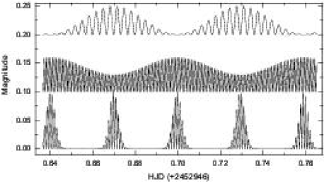
Figure 7: Plots of the test functions $F_{3}$ (upper), $F_{4}$ (middle) and $F_{5}$ (bottom), shifted by 0.1 in the y-direction.

Our model scalograms were generating using the same sampling that we had on our second night of observation. For the first test we generated artificial time-series by adding seven simulated signals using the following functions:

1. The simple sinusoid $F_{1}$ with constant semi-amplitude of 0.05 and frequency of $\nu_{1}=0.002$ Hz.

2. The sinusoid $F_{2}$ with constant semi-amplitude of 0.05, which frequency changes three times by a saltation (0.0145 Hz, 0.0150 Hz and 0.0155 Hz) at regular time intervals.

3. Two amplitude-modulated sinusoids $F_{3}$ and $F_{4}$ with frequencies $\nu_{3}$ and $\nu_{4}$ of 0.0035 Hz and 0.012 Hz respectively, and with frequency of amplitude modulations of $\nu_{orb}=1/P_{orb}=1.94\cdot 10^{-4}$ Hz. The amplitude of $F_{3}$ varies sinusoidally from 0 up to 0.05, while the amplitude of $F_{4}$ from 0.03 up to 0.06 (Fig. 7):

   $$F_{3}=\frac{0.05}{4}(1+\sin 2\pi\nu_{orb}t)(1+\sin 2\pi\nu_{4}t)$$ (4)

   $$F_{4}=\frac{1}{2}(0.045+0.015\sin 2\pi\nu_{orb}t)(1+\sin 2\pi\nu_{5}t)$$ (5)

4. One more amplitude-modulated sinusoid $F_{5}$ with frequency $\nu_{5}$ of 0.010 Hz and with an amplitude modulation frequency of 2 $\nu_{orb}=2/P_{orb}=3.89\cdot 10^{-4}$ Hz. Unlike the previous functions this sinusoid has visible oscillations (from 0 up to 0.10) for about 33% of the time (Fig. 7).

   We calculated it, using the following formula:

   $$F_{5}=0.05(\sin^{20}{2\pi\nu_{orb}t})\cdot(1+\sin{2\pi\nu_{6}t})$$ (6)

5. Two frequency-modulated sinusoids $F_{6}$ and $F_{7}$ with carrier frequencies $\nu_{c}$ of 0.0055 Hz and 0.0080 Hz respectively, and with modulating frequency $\nu_{m}$ of $1.62\cdot 10^{-4}$ Hz=$2/P_{phot}$ and $1.94\cdot 10^{-4}$ Hz=$1/P_{orb}$, respectively. The modulation index $\delta$ has been chosen so to obtain a maximum frequency deviation of 0.0008 Hz. The amplitude of both sinusoids are 0.05:

   $$F_{6,7}=0.05\sin(2\pi\nu_{c}t+\delta\sin{2\pi\nu_{m}t})$$ (7)

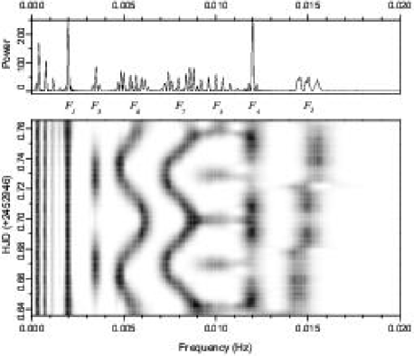
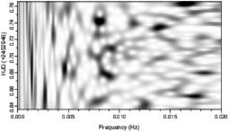
Figure 8: The Lomb-Scargle power spectrum (upper panel) and the scalogram (bottom panel) of the first artificial time-series. Frequency position of test functions are shown by $F_{1}$,…,$F_{7}$ (see text for explanation).

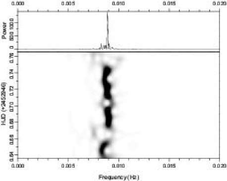
Figure 9: The scalogram of white noise.

Figure 10: The Lomb-Scargle power spectrum (upper panel) and the scalogram (bottom panel) of the AR(2) model with constants $a_{1}$=1.980 and $a_{2}$=–0.995.

Figure 10 shows the scalogram and the Lomb-Scargle power spectrum for the given artificial time-series. From this we can easily detect the basic characteristics of all seven input signals - frequency, duration, amplitude or frequency modulation, etc. In particular, a difference in the modulating frequencies $\nu_{m}$ of functions $F_{6}$ and $F_{7}$ is evident. However, we note a significant edge effect and reallocation of power along frequencies between various signals. As an example of the latter see that the brightness reduction of the vertical lines at frequencies of 0.0145–0.0155 Hz (function $F_{2}$) correlate with spots at 0.010 Hz (function $F_{5}$), as well as with different brightness of these spots along the time axis.

The first test time-series was without added noise. This was to determine the basic wavelet-transforms of the test functions. However the influence of noise on the scalograms is also of significant interest. Figure 10 shows the scalogram of discrete white noise having a normal distribution. Main distinctive feature of this scalogram is a honeycomb structure, as well as the concentrations of power, randomly distributed over scalogram. Though the latter have relatively low significance.

For an investigation of many processes interjacent between random and strictly periodic, Autoregressive Models AR($p$) can be used (Scargle, 1981):

$$x_{k}=a_{1}x_{k-1}+a_{2}x_{k-2}+...+a_{p}x_{k-p}+\xi_{k}$$ (8)

where $p$ is a model order, $a_{1},a_{2},...,a_{p}$ are model constants and $\xi_{k}$ is an uncorrelated white noise. As AR(2) models can have a quasi-sinusoidal appearance, they are particularly useful for representing quasi-periodic oscillations in accreting binaries. Our third test is devoted to obtaining the distinctive features of scalograms of AR(2) processes. For this we generated time-series for an AR(2) model with constants $a_{1}=1.980$ and $a_{2}=-0.995$. This model produces a narrow and very strong peak in its power spectrum (Fig. 10, upper panel) that can be mistakenly interpreted as an indication of coherent oscillations. However, wavelet analysis shows that it is definitely not. A strong line seen in the scalogram (Fig. 10, bottom panel), is not strictly vertical, though it is directed along the time axis. It can have frequency drifts, long enough sine-like parts, gaps, splits and confluences.

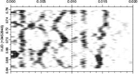
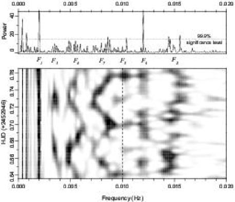
Figure 11: The slidogram (upper), the Lomb-Scargle power spectrum (middle) and the scalogram (bottom panel) of the first artificial time-series with added a white-Gaussian noise.

Finally we investigate how noise will distort slidograms and scalograms of periodic functions. For this we have used our first artificial time-series with added white-Gaussian noise with a mean of zero and a standard deviation $\sigma_{noise}$ of 0.1. The power spectrum of these noisy time-series (Fig. 11, middle panel) show only two test functions – $F_{1}$ and $F_{4}$, while the detection of other periodic signals is statistically insignificant. However, all seven test functions are evident in both the slidogram and scalogram. For example, a difference of the modulating frequencies $\nu_{m}$ of sinusoids $F_{6}$ and $F_{7}$ can again be detected, although the latter look more fragmentary, with a ”ragged” shape.

In conclusion we would like to point out some important features of the test function $F_{5}$ in the scalogram in the presence of noise. This function can be definitely detected, but the frequencies of its spots changes considerably, as well as their brightness. Occasionally some of them have completely disappeared. On the whole, the shorter the life of the function the bigger the variation in brightness and frequency.

References

- Dhillon & Marsh (2001) Dhillon V., Marsh T., 2001, NewAR, 45, 91
- Foster (1996) Foster G., 1996, AJ, 112, 1709
- Gabor (1946) Gabor D., 1946, J. Inst. Elec. Eng. (London), 93, 429
- Hakala et al. (2004) Hakala P., Ramsay G., Wheatley P., Harlaftis E. T., Papadimitriou C., 2004, A&A, 420, 273
- Haubold (1997) Haubold H. J., 1997, Ap&SS, 258, 201
- Hoffmeister (1949) Hoffmeister C., 1949, Veroff. Sternw. Sonneberg 1, 3
- Leins et al. (1992) Leins M., Soffel M. H., Lay W., & Ruder H., 1992, A&A, 261, 658
- Lomb (1976) Lomb N. R., 1976, Ap&SS, 39, 447
- Mallat (1987) Mallat S., 1987, Proc. IEEE Computer Society Workshop on Computer Vision, (Washington DC: IEEE Computer Society Press), 2
- Misselt (1996) Misselt K. A., 1996, PASP, 108, 146
- Neustroev (2002) Neustroev V. V., 2002, A&A, 382, 974
- Press et al. (1992) Press W. H., Teukolsky S. A., Vetterling W. T., Flannery B. P., 1992, Numerical Recipes, 2nd ed. (Cambridge: Cambridge University Press), 570
- Roberts, Lehar, & Dreher (1987) Roberts D. H., Lehar J., Dreher J. W., 1987, AJ, 93, 968
- Scargle (1981) Scargle J. D., 1981, ApJS, 45, 1
- Scargle (1982) Scargle J. D., 1982, ApJ, 263, 835
- Schulz & Mudelsee (2002) Schulz M., Mudelsee M., 2002, Computers & Geosciences, 28, 421
- Schulz & Stattegger (1997) Schulz M., Stattegger K., 1997, Computers & Geosciences, 9, 929
- Smith et al. (2002) Smith J. A., et al., 2002, AJ, 123, 2121
- Szatmary, Vinko, & Gal (1994) Szatmary K., Vinko J., Gal J., 1994, A&AS, 108, 377
- Thorstensen et al. (1996) Thorstensen J.R., Patterson J.O., Shambrook A., Thomas G., 1996, PASP, 108, 73
- Tovmassian et al. (2003) Tovmassian G., Zharikov S., Michel R., Neustroev V., Greiner J., Skillman D. R., Harvey D. A., Fried R. E., Patterson J., 2003, PASP, 115, 725
- Tovmassian & Zharikov (2004) Tovmassian G., Zharikov S., 2004, RevMexAC, 20, 169
- van Zyl et al. (2004) van Zyl L., et al., 2004, MNRAS, 350, 307
- Vityazev (2001) Vityazev, V. V., 2001, Wavelet Analysis of Time Series, St.-Petersburg (in Russian)
- Warner (1995) Warner B., 1995, Cataclysmic Variable Stars (Cambridge Astrophysics Ser. 28; Cambridge: Cambridge Univ. Press)
- Warner & Brickhill (1978) Warner B., Brickhill A. J., 1978, MNRAS, 182, 777
- Woudt & Warner (2002) Woudt P. A., Warner B., 2002, Ap&SS, 282, 433
- Woudt, Warner, & Pretorius (2004) Woudt P. A., Warner B., Pretorius M. L., 2004, MNRAS, 351, 1015
- Zharikov et al. (2005) Zharikov S. V., Tovmassian G. H., Neustroev V., Michel R., Napiwotzki R., 2005, in The Physics of Cataclysmic Variables and Related Objects, ed. Hameury J.-M. & Lasota J.-P. (ASP Conf. Ser. 330), 327