Fate of a neutron star with an endoparasitic black hole and implications for dark matter

Abstract

We study the dynamics and observational signatures of a neutron star being consumed by a much less massive black hole residing inside the star. This phenomenon could arise in a variety of scenarios, including after the capture of a primordial black hole, or in some models of asymmetric dark matter where the dark matter particles collect at the center of a neutron star and eventually collapse to form a black hole. However, the details of how the neutron star implodes are not well known, which is crucial to determining the observational implications of such events. We utilize fully general relativistic simulations to follow the evolution of such a black hole as it grows by several orders of magnitude, and ultimately consumes the neutron star. We consider a range of spin values for the neutron star, from nonrotating stars to those with millisecond periods, as well as different equations of state. We find that as the black hole grows, it obtains a non-negligible spin and induces differential rotation in the core of the neutron star. In contrast to previous studies, we find that the amount of dynamical ejecta is very small, even for rapidly rotating stars, dampening the prospects for producing a kilonova-type electromagnetic signal from such events. We comment on other possible electromagnetic and gravitational signals.

I Introduction

Recently, there has been much interest in scenarios where neutron stars (NSs) capture dark matter—either particles or primordial black holes (BHs)—giving rise to a tiny BH which consumes the NS from the inside through accretion. This could give rise to a number of observable consequences, allowing NSs to play the role of dark matter detectors, while addressing several astrophysical mysteries, as we review below.

This phenomenon could arise due to bosonic or fermionic asymmetric dark matter Goldman and Nussinov (1989); de Lavallaz and Fairbairn (2010); Kouvaris and Tinyakov (2011); McDermott et al. (2012); Bramante and Linden (2014); Bramante and Elahi (2015). The dark particles are captured by the NS due to neutron scattering, and if their annihilation and decay rates are sufficiently small, they will eventually thermalize and collect to form a tiny ($\lesssim 10^{-10}\ M_{\odot}$) BH at the NS center Goldman and Nussinov (1989); Bramante et al. (2018). Similarly, if primordial BHs with masses $\sim 10^{-14}$–$10^{-8}\ M_{\odot}$ make up a fraction of the dark matter, they will be captured onto NSs through dynamical friction and accretion Capela et al. (2013). In either case, the BH should grow through accretion until it consumes the NS.

The BH-induced implosion of NSs, which would preferentially occur in regions of high dark matter density, has been invoked as a possible explanation for the scarcity of observed pulsars in the Galactic center Bramante and Linden (2014). It has also been proposed that this could give rise to fast radio bursts (FRBs) due to the rapid expulsion of the NS magnetosphere Fuller and Ott (2015) (though this type of cataclysmic event cannot explain repeating FRBs). Finally, in Refs. Bramante and Linden (2016); Fuller et al. (2017), it was proposed that ejecta from the imploding NS could explain the production of the majority of heavy elements through the r process.

There are several observational signatures that could be used to identify such events. One would be the presence of $\sim 1\ M_{\odot}$ BHs in binary merger events detected by LIGO/Virgo and other gravitational wave (GW) observatories (though NS implosions may not be the only conceivable explanation). Actually distinguishing BHs from NSs of the same mass with the merger GW signal is challenging because tidal effects are significant only in the high frequency part of the signal where current detectors are not very sensitive Abbott et al. (2017), and because if at least one of the constituents of the binary is a NS, there is a degeneracy in the leading order tidal effect due to our ignorance about the equation of state (EOS) describing NSs Yang et al. (2018). If detected, electromagnetic counterparts to such GW signals could be used to provide strong evidence of the presence of a NS, though ruling out a BH-NS binary is more difficult Yang et al. (2018); Hinderer et al. (2018); Foucart et al. (2019).

Another possible signature coming from the collapse of a NS to a BH is a kilonova: an IR/optical/UV transient powered by the radioactive decay of ejected, neutron-rich material. However, the amount of ejecta depends crucially on the dynamics of process, and on the distribution of angular momentum as the BH grows, which is not well understood. Most previous studies have left this amount as an unknown, bounded above by measurements of the total abundance of r-process elements. An exception to this is Ref. Fuller et al. (2017), where it was estimated that the collapse of a millisecond period NS could produce $\sim 0.1$ to $0.5\ M_{\odot}$ in ejecta, a range of values in excess of those found in binary NS mergers Siegel (2019).

Several works have estimated the timescales and relevant physical processes involved during the months to years-long period where the BH grows through accretion inside the NS, but has negligible effect on the star as a whole. (We note that for the BH mass ranges mentioned above, the Hawking evaporation time is much longer than the age of the Universe.) In Refs. Kouvaris and Tinyakov (2014); Fuller et al. (2017), building from the related problem of a BH inside a solar-type star Markovic (1995), it was argued that the effects of nuclear viscosity and magnetic braking would be important. Based on Newtonian estimates, these works contend that spherical (i.e. Bondi-like) accretion is maintained throughout the whole consumption process. Such behavior is governed by sheer viscous braking for BH masses $\lesssim 10^{-3}M_{\odot}$, and magnetic braking for larger masses.

In this work, we study how the BH grows from a mass that is small, but near becoming dynamical important—we begin our analysis when the BH is roughly a hundredth of the NS mass—,to ultimately consume the majority of the NS, a process which occurs over a few milliseconds. We explore several initial conditions based on uniformly rotating star solution—thus making contact with previously mentioned estimates but studying its future evolution within general relativity. We use solutions of the coupled Einstein-hydrodynamics equations, which allows us to follow the relativistic dynamics as the BH begins to backreact on the rotating NS, and make accurate estimates of potential observational signatures. The large disparity between the length scales respectively associated with the NS and BH makes this a computationally challenging problem, which we overcome through a combination of several techniques, including the use of adaptive mesh refinement with flux corrections for the hydrodynamics, and by exploiting spacetime symmetries.

We find that the BH develops and maintains a non-negligible spin, and induces differential rotation in the core of the NS, and we give a simple heuristic description for the accretion of angular momentum as the BH grows. The rate of mass accretion, however, is largely insensitive to angular momentum. We show that essentially no matter remains outside the BH horizon at the end of the process, even for NSs rotating at speeds near breakup, which means that these events are not promising sources for kilonovae or r-process heavy elements. We comment on possible GW and electromagnetic signatures, including bursts from the sudden release of the energy stored in the NS’s magnetosphere.

II Methodology

In order to study the dynamics of a rotating NS being consumed by a BH from the inside, we solve the Einstein equations coupled to hydrodynamics. To construct initial data, we begin with a uniformly rotating NS solution obtained using the RNS code Stergioulas and Friedman (1995). We then alter this solution in a neighborhood of the center of the star to match on to a small BH metric with a quasiequilibrium test fluid. We use this as free data for solving the Einstein constraint equations as described in Ref. East et al. (2012a). Though this solution is only an approximate description of the system of interest, we have tested several initial values for the BH mass $M_{\rm BH}$ in order to establish that we start with a sufficiently small value that any initial transients are negligible. More details are provided in Appendix A.

The evolution is carried out using the methods (and code) described in Ref. East et al. (2012b). This includes the use of adaptive mesh refinement with flux corrections Berger and Colella (1989), which ensure that the conservative nature of the hydrodynamic evolution scheme is not broken by the numerous levels of mesh refinement with boundaries inside the NS which are required to resolve the BH. The hydrodynamic scheme conserves rest mass and, in axisymmetry, angular momentum.

We fix the NS to have a mass of $M_{\rm NS}=1.4\ M_{\odot}$ and consider three different EOSs. We use the SLy and ENG EOS, which are “softer” and give radii of 11.7 and 12 km, respectively, for a nonrotating NS. We also use the stiffer H4 EOS, which gives a radius of 14 km for a nonrotating NS, and is at the edge of the allowed range consistent with the binary NS merger GW170817 Abbott et al. (2018). In particular, we use the piecewise polytrope approximation of these EOSs described in Ref. Read et al. (2009). As we describe below, the systems we consider develop densities in the vicinity of the accreting BH that are larger than the maximum density of isolated NSs (even ones of $\sim 2\ M_{\odot}$), and the softer EOSs, when extrapolated to these values, would give superluminal sound speeds. To address this, at the value of the rest-mass density when the sound speed becomes $c_{s}\approx 0.99$ ($\rho_{0}=1.43\times 10^{15}$ gm/cm³ for ENG; $\rho_{0}=1.96\times 10^{15}$ gm/cm³ for SLy), we match onto an EOS with $c_{s}$ held constant at this value. (Unless otherwise specified, we use geometric units with $G=c=1$ throughout.) To this cold EOS, we also add a thermal component with $P_{\rm hot}=0.5\rho_{0}\epsilon_{\rm hot}$, where $\epsilon_{\rm hot}=\epsilon-\epsilon_{\rm cold}$ is the specific energy is excess of the value prescribed by the cold EOS Bauswein et al. (2010). However, we find that in all the cases we study, shock heating effects are not significant.

Table 1:

Properties of equilibrium uniformly rotating NSs used to construct ID. Left to right, the columns contain the EOS, dimensionless NS spin, rotational period, equatorial radius, and ratio of angular velocity to that of a particle orbiting at the equator. EOS $a_{\rm NS}$ Period (ms) $R_{\rm eq}$ (km) $\Omega/\Omega_{K}$ ENG 0.00 — 12.0 0.00 ENG 0.10 5.3 12.0 0.12 ENG 0.20 2.7 12.2 0.23 ENG 0.40 1.5 12.9 0.47 ENG 0.70 1.0 16.5 0.95 H4 0.00 — 14.0 0.00 H4 0.10 6.6 14.0 0.12 H4 0.20 3.4 14.2 0.23 H4 0.40 1.8 15.1 0.47 H4 0.67 1.3 18.7 0.89 SLy 0.00 — 11.7 0.00 SLy 0.20 2.6 11.9 0.24 SLy 0.40 1.4 12.7 0.48

For each EOS, we consider a range of values for the dimensionless NS spin $a_{\rm NS}$, from nonspinning to millisecond period NSs near breakup, as shown in Table 1. For most cases, and unless otherwise stated, we choose the initial BH to have mass $M_{\rm BH}=10^{-2}M_{\rm NS}$ and dimensionless spin $a_{\rm BH}=a_{\rm NS}$, and we assume axisymmetry. Here and throughout we use $M_{\rm NS}$ to refer to the total mass of the spacetime, which is equal to the NS mass before the BH obtains a non-negligible mass. For the case with the ENG EOS and $a_{\rm NS}=0.4$, we consider several variations as a check of our initial conditions and numerical errors. We study larger initial BHs with $M_{\rm BH}/M_{\rm NS}=0.02$ and 0.03. We examine different initial BH spins with $a_{\rm BH}=0$, 0.2, and 0.4. To establish convergence and estimate numerical errors, we also adopt several numerical resolutions (with $a_{\rm BH}=0.4$ and $M_{\rm BH}/M_{\rm NS}=10^{-2}$). Finally, we consider one case calculated without assuming any spatial symmetries, starting from initial conditions from the axisymmetric simulations at the time when $M_{\rm BH}/M_{\rm NS}=0.05$, in order to check for nonaxisymmetric instabilities. As detailed in Appendix B, in all cases we obtain similar results.

During the evolution, we track the BH apparent horizon and monitor its area $A_{\rm BH}$ and angular momentum (from which the BH mass $M_{\rm BH}$ and dimensionless spin $a_{\rm BH}$ is calculated, via the Christodoulou formula). We also calculate the flux of conserved matter quantities into the horizon: the rest-mass accretion rate $\dot{M}_{0}$ and the angular momentum accretion rate $\dot{J}$.

We also determine the amount of unbound rest mass by integrating all the fluid cells where the lower time component of the four velocity $u_{t}<-1$, and the radial component of the velocity is outward, as is typically done in NS merger simulations.

III Results

Starting from one one-hundredth the mass of the NS, we find that the “endoparasitic” BH efficiently grows to consume essentially the entire NS in $\approx 4$–6 ms. As shown in the top panel of Fig. 1, the accretion rate of the BH is mostly determined by the NS EOS. The spin of the NS has only a small effect on the growth rate of the BH, with higher spins giving slightly slower growth rates. The spin of the NS does, however, affect the BH spin. As evident in the bottom panel of Fig. 1, $a_{\rm BH}$ settles to a value of $\sim a_{\rm NS}/2$, and roughly maintains this value as the BH mass grows more than an order of magnitude. At the last stages of the NS being consumed, $a_{\rm BH}$ jumps up to match $a_{\rm NS}$.

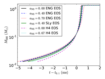
Figure 1: Top: The mass of the BH as a function of time for cases with different spins and EOSs for the NS. The curves have been aligned at the time where $M_{\rm BH}=0.1M_{\rm NS}$. Bottom: The dimensionless spin of the BH versus its mass.

The BH accretion follows the Bondi relation $\dot{M}_{0}\propto A_{\rm BH}$ to a very good approximation all the way up to $M_{\rm BH}\sim M_{\rm NS}/2$ as illustrated in the top panel of Fig. 2, and the differences between the accretion rates with different EOSs fall into line with what one expects from evaluating the central values of $\rho_{0}/c_{s}^{3}$ for the respective isolated NS solutions (also consistent with Bondi). Again, the matter accretion rate is largely independent of the NS spin.

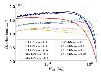
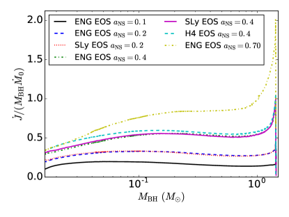
Figure 2: Top: The rest-mass accretion rate for the BH, normalized by the area of the BH. For comparison, the central value of $\rho_{0}/c_{s}^{3}$ is $1.1\times$ ($1.7\times$) higher for a nonspinning NS with the SLy EOS (H4 EOS) compared to the ENG EOS, which correlates with the difference in accretion rate. Bottom: The ratio of the angular momentum to rest-mass accretion rate for the BH, normalized by the mass of the BH. For both cases the quantities are shown versus the mass of the BH as it grows.

More interesting is the rate at which angular momentum is accreted relative to rest mass, as shown in the bottom panel of Fig. 2. To a good approximation, we find that this ratio $\dot{J}/\dot{M}_{0}$ is linearly proportional to the BH radius, or equivalently, mass, throughout most of its growth. This is consistent with the above-noted fact that the BH spin settles down to a roughly constant value as the BH grows [in such a regime $dJ_{\rm BH}=d(M_{\rm BH}^{2})a_{\rm BH}$]. In particular, if we assume that the BH angular momentum changes as $\delta J_{\rm BH}=\alpha M_{\rm BH}\delta M_{\rm BH}$ for some constant $\alpha$, then $\delta a_{\rm BH}=\delta M_{\rm BH}(\alpha-2a_{\rm BH})/M_{\rm BH}$, i.e. $a_{\rm BH}$ will have a stable equilibrium value at $\alpha/2$. Figure 2 indicates that this proportionality constant is relatively insensitive to the EOS.

Examining the angular dependence of the flux through the BH horizon, we find the rest-mass accretion to be approximately spherical, while the ratio of the angular momentum to rest-mass accretion rate of an area element on the BH horizon is approximately proportional to $\sin^{2}\theta$ (where $\theta$ is the polar angle), all consistent with the BH accreting spherical shells of mass, uniformly rotating with angular velocity $\Omega$ (i.e. the coordinate velocity in the azimuthal direction). With this assumption, the condition that $\dot{J}/\dot{M}_{0}\propto R_{\rm BH}$ is equivalent to $\Omega\propto 1/R_{\rm BH}$. Such a relation would follow from assuming Keplerian velocity, or taking $\Omega$ to be proportional the horizon frequency of a BH with constant dimensionless spin, though it is inconsistent with the uniform rotation of the original star. See Appendix C for further discussion.

Indeed, we find that the BH induces differential rotation in the NS, as apparent from Fig. 3, which shows snapshots of the density and angular velocity. There we see that the central core of the NS rotates much faster compared to the outer part, which does not significantly increase from its original rotation value. Also evident from Fig. 3 is the high density that develops in the vicinity of the BH. At the BH horizon we find $\rho_{0}\gtrsim 2\times 10^{15}$ gm/cm³. As mentioned above, these densities are 2–$3\times$ larger the initial central densities of the NS, and higher even than those obtained for the maximum stable NS solutions with their respective EOSs. In the final phase of the NS implosion for the near breakup spin case with $a_{\rm NS}=0.7$ (bottom-right panel of Fig. 3), one can see spherical accretion beginning to break down as the region near the rotation axis is evacuated first, and the high angular momentum material near the equator is the last to be accreted. This is consistent with the late-time decrease in mass accretion rate, coupled with an increase in relative angular momentum accretion rate, shown in Fig. 2.

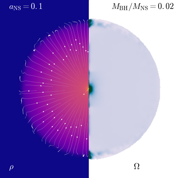
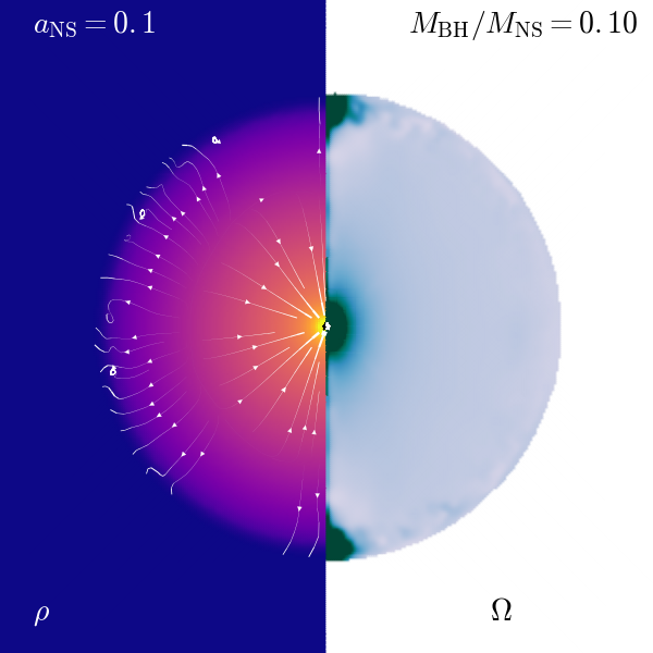
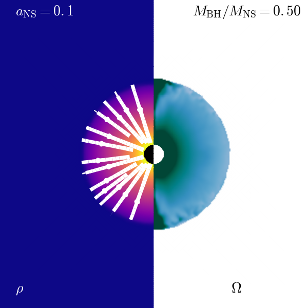
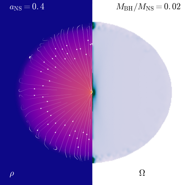
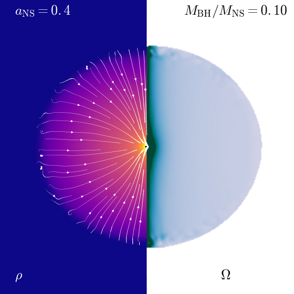
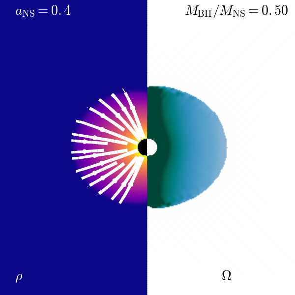
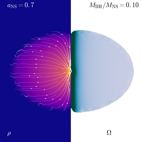
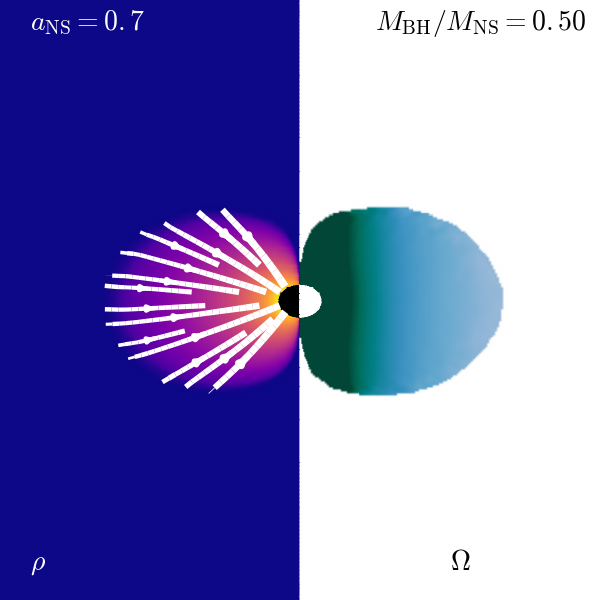
Figure 3: Snapshots of density and angular velocity during the evolution of cases with the ENG EOS and different NS spins. The left side of each snapshot shows the rest-mass density (on a linear scale from 0 to $1.6\times 10^{15}$ gm/cm³) with streamlines of the in-plane component of the velocity (with line width proportional to their magnitude), while the right side shows the angular velocity about the axis of symmetry. The top panels are from the case with $a_{\rm NS}=0.1$, and respectively show, from left to right, the points in the evolution when the BH has grown to be 0.02, 0.1, and 0.5 times the mass of the original NS. The middle and bottom panels show the same for the cases with $a_{\rm NS}=0.4$ and 0.7, respectively. The color scale for the angular velocity is linear, ranging from 0 to $4\times$ the initial angular velocity of the NS. At earlier times, the small radial velocities at the outer parts of the star are due to breathing modes.

A more quantitative illustration of the differential rotation on the equator is shown for several cases with different EOSs and NS spins in Fig. 4. Here, we see that the rotation curves do not depend strongly on the EOS, and match up well when normalized by $\Omega_{\rm NS}$. In Fig. 4, we also include the best fit of the azimuthal angular velocity to the functional form $\Omega=A+B/r^{n}$. At earlier times (i.e. when the BH mass is small), this exponent $n\sim 2$, though at late times $n$ becomes smaller. As a point of comparison, we note that the angular velocity of a viscous fluid between two concentric spheres rotating with different velocities has this form with $n=3$ Landau and Lifshitz (1987). The figure also makes apparent the fact that the rotation rate at the accreting radius decreases, while at the star’s surface it increases. The former is expected as the angular frequency of the BH is $\Omega_{H}=a/(2R_{BH})$—which decreases as the BH grows. Indeed, we find good agreement with this behavior as indicated in the figure. We also find that the rotation rate at the surface increases as the NS radius shrinks, roughly following the $\Omega_{s}\propto R_{\rm NS}^{-2}$ behavior predicted from assuming the angular momentum of the outer shell is constant. The change in $\Omega_{s}$ is only significant at the last stages of the implosion, where it is accompanied by the contraction of the star, and a strong inward radial velocity (see Fig. 3).

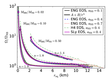
Figure 4: The angular velocity on the equator as a function of proper circumferential radius. For each case with different EOS or NS spin, we show the rotation curve at three different times, corresponding, respectively, to when the BH has grown to have 0.02, 0.1 and 0.5 times the mass of initial NS. We also show fits of the form $\Omega=A+B/r_{\rm eq}^{n}$ to the case with ENG EOS and $a_{\rm NS}=0.4$ (though other cases give similar results). The exponent $n$ of the best-fit is found to decrease from $\sim 1.9$ to 1.4, as labeled in the plot. For the SLy EOS and $a_{\rm NS}=0.4$ case, we also include the values of the BH horizon frequency $\Omega_{H}$ for comparison (magenta dots).

As a consequence of the distribution of angular momentum during the BH growth described above, almost no matter is dynamically ejected. In some of the cases with higher spin, we find a few $\times 10^{-5}\ M_{\odot}$ of rest mass, flagged as unbound. However, this is sensitive to extraction time, and seems likely to be coming from the low density region outside the NS, rather than being ejected from the NS’s surface. Given the difficulty in resolving the behavior in the very low density region, especially in the presence of an artificial “atmosphere,” we cannot rule out a very small amount of unbound mass, but we estimate an upper bound of $M_{\rm ub}<10^{-4}\ M_{\rm\odot}$. (See Ref. Camelio et al. (2018) for a discussion of these issues in a study of supramassive NS collapse using similar methods.)

Finally, we examine the GW signal from this process. Though there will be no GWs from the collapse of a NS into a BH in spherical symmetry, when there is non-negligible NS spin there will be gravitational radiation associated with the quadrupole of the NS changing into that of a spinning BH. In Fig. 5, we can see that the GW signal exhibits the standard ringdown signal associated with a perturbed BH, with larger amplitudes for the larger spin cases. Unfortunately, the high characteristic frequency ($8$–$9$ kHz) of the GW signal makes it difficult to detect with current GW detectors. LIGO/Virgo would likely only be able to detect such an event in the Milky Way or a nearby satellite galaxy (at distances of a few $\times 10$ kpc). Though the GW amplitude is comparable to NSs induced to collapse by other mechanisms Duez et al. (2006); Baiotti et al. (2007); Giacomazzo et al. (2011), the frequency is generally higher compared to a NS collapsing because it has exceeded the maximum supported mass (e.g. through accretion).

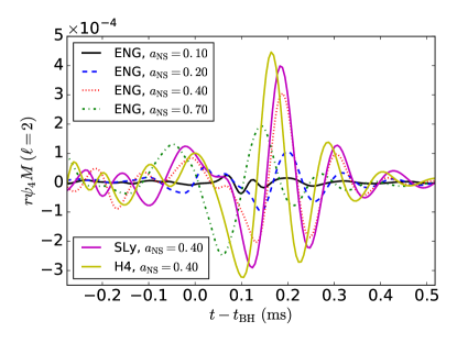
Figure 5: The GW signal, in particular the $\ell=2$, $m=0$ component of $\psi_{4}$, for the collapse of different NSs. The curves have been aligned in time to the look-back time where the BH reaches $95\%$ of the mass of the spacetime.

Other electromagnetic counterparts

Having found that the BH consumes the whole NS without giving rise to any appreciable ejecta, we briefly comment on possible electromagnetic transients powered by other means. A NS is generically magnetized with field strengths of order $B\simeq 10^{8}$ to $10^{12}$ G. No hair theorems imply that as the spacetime approaches that of a vacuum BH, this magnetic field must go away. Some of the magnetic field energy falls into the BH horizon, but the study presented in Ref. Lehner et al. (2012) shows that a significant amount is radiated to infinity on dynamical timescales, giving rise to a transient signal. The energy reservoir for such a signal is that of the NS magnetosphere, which is of the order

$$E_{M}\approx 2\times 10^{37}\left(\frac{B}{10^{10}\ \rm G}\right)^{2}\left(\frac{R}{10\ {\rm km}}\right)^{3}\mbox{erg}\ .$$ (1)

As discussed in Ref. Lehner et al. (2012), a fair fraction of this energy is released on timescales of $\approx 1$ ms as a result of the collapse of the NS to a BH, resulting in a short burst with a luminosity of

$$L\approx 6\times 10^{39}\left(\frac{\kappa}{0.6}\right)\left(\frac{B}{10^{10}\ \rm G}\right)^{2}\left(\frac{R}{10\ {\rm km}}\right)^{3}\mbox{erg/s}$$ (2)

where $\kappa\approx 0.6$ is an efficiency factor. The associated Poynting flux follows an essentially quadrupolar distribution with most of the energy radiated near the angles $\theta=\pm 50^{o}$. The environments surrounding pulsars typically have relatively low baryon loading. The details of how this energy is converted into specific observable signatures are certainly model dependent (see, for instance, Refs. Lehner et al. (2012); Falcke and Rezzolla (2014) for options ranging from short gamma-ray to radio bursts). Regardless, an electromagnetic transient with these characteristics that lacks an associated kilonova is arguably a clear signature of the NS implosions studied here. As mentioned above, it is possible that for sufficiently close systems, multimessenger signals in both gravitational and electromagnetic bands could be detected. Notice that NSs driven to collapse by accreting matter from a companion or (for massive ones) angular momentum loss through spin down would also emit in analogue ways. However, there are subtle differences that could allow for discerning whether such signals come from the mechanism discussed here, or these “standard” ones. First, since the frequencies of GWs are strongly correlated with the mass of the collapsing star, they would reveal whether such a star is clearly below its maximum mass, thus favoring the endoparasitic mechanism. Second, such a mechanism preferentially takes place in regions with higher dark matter density. Finally, a collapsing NS within the standard scenario explores higher temperatures, and thus is more likely to produce neutrinos.

IV Discussion and Conclusion

We have studied the process by which a small seed BH in the center of a rotating NS grows, and ultimately consumes the star. In this endoparasitic process, even for NSs with very short rotational periods, exceeding observed values, very little of the star’s material remains outside the BH ($M_{\rm ub}<10^{-4}\ M_{\rm\odot}$). This contrasts with the estimates of $M_{\rm ub}\sim 0.1$–$0.5\ M_{\rm\odot}$ presented in Ref. Fuller et al. (2017). There it was assumed that the total angular momentum would be distributed to the solid shell of the star, which would maintain rigid rotation down to the BH horizon, plus an outer angular shell, which could become unbound once a high enough velocity was achieved, and that a negligible amount of angular momentum would go into the BH. In contrast, we find that the BH obtains a non-negligible spin, and is surrounded by differentially rotating core with much higher angular velocity than the outer part of the NS. Furthermore, as the BH grows by a significant amount a rather cylindrical distribution of angular momentum is found in cases with initial higher rotational velocity. Such behavior is consistent with the development of Ekman layers Proudman (1956). For the highest NS spin considered here ($a_{\rm NS}=0.7$), at late times an evacuated “funnel” region results. This behavior is expected as such a region lacks the angular momentum support to resist prompt accretion, and is thus consumed more rapidly than the lower latitude regions.

Here we restricted to a hydrodynamical treatment of the NS, and ignored the effect of viscosity, magnetic fields, etc. The main justification for this is the very short timescales in between when the BH becomes large enough to have a significant effect on the NS as a whole, and when the NS is completely gone. As shown here, even for EOSs with high sound speeds that give lower accretion rates, once the BH has consumed $1\%$ of the NS’s mass, it only takes milliseconds for it to consume the rest. The effects of sheer viscosity and magnetic braking have been studied in scenarios related to ours Markovic (1995) in the context of a potential BH in the Sun, and adapted for the NS case in Refs. Kouvaris and Tinyakov (2011); Fuller et al. (2017). Sheer viscosity is deduced to affect the angular rotation while $M_{\rm BH}\lesssim 10^{-3}\ M_{\odot}$, with magnetic braking becoming the relevant effect afterwards. These works conclude that the viscosity and magnetic braking ensure that rotation does not halt the infall of matter into the BH, and both Bondi accretion and uniform rotation are preserved through essentially the full lifetime of the consumption process. Notice Newtonian estimates miss, in particular, dragging by the BH’s rotation and the accretion process itself. Furthermore, during the rapid evolution ensuing after the BH mass satisfies $M_{\rm BH}\gtrsim 10^{-2}\ M_{\odot}$, the Alfvén timescale $\tau_{B}\simeq(10^{12}\ {\rm G}/B)$ s becomes too long for magnetic braking to operate efficiently. Our hydrodynamical calculations, which begin when the BH mass is already a hundredth of the NS mass with uniform rotation for the NS, are thus a realistic representation of the state the preceding dynamics—beginning with a BH seed with mass $\lesssim 10^{-8}M_{\odot}$—should give rise to.

We carried out a thorough study of different initial values for the BH mass and spin (see Appendix A), which we find all give similar results. Moreover, we argue that our results should extrapolate to smaller BH masses (at least until other processes which we neglect here, e.g. magnetic braking or viscosity, become important) based on the simple power law scaling relationships we observe for the rates of accretion of mass and angular momentum with the BH mass (approximately $\dot{M}_{0}\propto M_{\rm BH}^{2}$ and $\dot{J}\propto M_{\rm BH}^{3}$), which we find hold until the very final stages of the NS implosion, and which give nearly constant dimensionless BH spin.

Our results put a damper on the “quiet kilonovae” scenario for observing NS implosions—i.e. a kilonovae that is not accompanied by the significant GW signal of a BH-NS or NS-NS merger—as well as for placing bounds on their rates through the abundance of r-process material. However, several observational possibilities still remain. We predict that this mechanism should produce a population of BHs whose mass and angular momentum distribution should tightly match that of the NSs which gave rise to them. If these BHs were to subsequently merge with a compact object companion, as discussed in the introduction, their BH nature could in principle be deduced from the GW signal and/or electromagnetic counterpart (or lack thereof). In principle, the GW signal from the NS implosion itself would encode the mass and spin of the newly formed BH (and distinguish from NSs collapsing due to becoming too massive), and could be observed with current detectors within our own Galaxy or nearby. Future GW detectors, especially those targeting the kilohertz frequency band Martynov et al. (2019), could improve this.

As also discussed, a magnetized NS has to shed its magnetosphere upon conversion to a BH, which leads to an electromagnetic outburst on millisecond timescales, though with unknown frequency. An interesting avenue for future work would be to include magnetic fields in a study similar to this one, in order to track the possible enhancement due to the differential rotation of the NS, and better model the release of the electromagnetic energy as the BH grows large. Energetically, such events are plausible sources for FRBs, and even short gamma-ray bursts, which would be unaccompanied by a kilonova. New observatories like CHIME Amiri et al. (2019), HIRAX Newburgh et al. (2016), SKA Carilli and Rawlings (2004), FAST Nan et al. (2011), and others are rapidly increasing the number of observed FRBs, and providing crucial clues to their source(s). Upcoming radio surveys will also take a more accurate census of the pulsar population in the galactic core, which will place bounds on, or provide evidence for, the scenario studied here. Likewise, gamma-ray detectors like Fermi, VERITAS, MAGIC, and HAWC Goldstein et al. (2017); Albert et al. (2018); Abeysekara et al. (2018); Archer et al. (2019) could potentially help identify these events.

Finally, we mention that it is intriguing that these systems probe higher densities than even massive NSs, about an order of magnitude above nuclear density, with this high density persisting during the accretion phase. Though it is unclear whether there will be any special observational signature (e.g., through neutrino seismology), since the material is in the process of falling into the BH, the behavior of matter at these densities is highly unknown, and may not be otherwise probed.

V Acknowledgements

We thank Joe Bramante for helpful discussions. W.E. and L.L. acknowledge support from an NSERC Discovery grant. L.L. acknowledges CIFAR for support. This research was supported in part by Perimeter Institute for Theoretical Physics. Research at Perimeter Institute is supported by the Government of Canada through the Department of Innovation, Science and Economic Development Canada and by the Province of Ontario through the Ministry of Research, Innovation and Science. This research was enabled in part by support provided by SciNet (www.scinethpc.ca/) and Compute Canada (www.computecanada.ca).

Appendix A Details of initial conditions

In this section, we give details on the initial data we use to describe a rotating NS with an interior BH. We construct solutions to the Einstein constraint equations by solving the conformal thin-sandwich equations as described in Ref. East et al. (2012a). We choose the free data for these solutions by combining a uniformly rotating NS solution with mass $M_{\rm NS}$ and dimensionless spin $a_{\rm NS}$, obtained using the RNS code Stergioulas and Friedman (1995), with a rotating BH solution with mass $M_{\rm BH}$ and dimensionless spin $a_{\rm BH}$, in Kerr-Schild coordinates, as we describe below.

We begin with a NS solution in spherical-polar type coordinates with the radial coordinate $R$ chosen such that $2\pi R\sin\theta$ is the proper circumference of any point rotated around the axis of symmetry. We choose a radius $R_{m}$ where we match on to the BH solution, and rescale the time coordinate of the NS solution by a constant factor so that is agrees with the value for the lapse for a Boyer-Lindquist BH on the equator at $R_{m}$. Then we apply the coordinate transformation that goes from Boyer-Lindquist to Cartesian Kerr-Schild coordinates for a BH with parameters $M_{\rm BH}$ and $a_{\rm BH}$ to the NS solution to obtain the metric $g_{\rm ab}^{NS}$. We combine this metric with the BH metric in Kerr-Schild coordinates using a transition function: $g_{ab}=f(R)g^{\rm NS}_{ab}+\left[1-f(R)\right]g^{\rm BH}_{ab}$ (since in the absence of spherical symmetry, the two solutions do not agree at $R=R_{m}$) with $f(R)=T\left((R-R_{m}+\delta R)/(2\delta R)\right)$ and where

$$T(x)=\left\{\begin{array}[]{lll}0&\mbox{if }x<0\\ x^{3}(6x^{2}-15x+10)&\mbox{if }0\leq x\leq 1\\ 1&\mbox{if }x>1\end{array}\right.$$ (3)

interpolates between 0 and unity with continuous first and second derivatives. Finally, we rescale the time coordinate of the combined solution by an overall factor so that the lapse goes to unity at spatial infinity. From this solution we calculate the free data metric functions. We want $R_{m}$ to be intermediate in scale between the BH and the NS radius, and $\delta R$ to be intermediate in scale between the BH radius and $R_{m}$, though the resulting dynamics are not very sensitive to the exact values. We use $R_{m}\approx 40M_{\rm BH}$ and $\delta R=0.1R_{m}$.

Similarly for the matter, we combine the density and velocity profile of the rotating NS solution with a quasiequilibrium test fluid solution on the BH background. For the latter, we assume constant $hu_{t}$ (where $h=1+\epsilon+P/\rho_{0}$ is the specific enthalpy), where the constant value comes from the NS solution at $R=R_{\rm m}$ on the equator. We also assume the same constant angular velocity throughout. Very near the BH ($R<3M_{\rm BH}$), we set the density to 0. Again, we combine these two solutions using the same transition function, e.g. $\rho_{0}=f(R)\rho_{0}^{\rm NS}+\left[1-f(R)\right]\rho_{0}^{\rm BH}$. From this, we calculate the conformal energy and momentum density, which are used in solving the conformal thin-sandwich equations.

The corrections we find from solving the constraints are small; e.g. the maximum difference from unity of the conformal factor over the domain is $\max|\Psi-1|\sim 0.01$. There is an initial transient when evolving these solutions since, for example, we do not include an inward radial velocity. However, we find the solution settles down to steady accretion in a few sound crossing times. We verify that our initial data are good enough, and that we start sufficiently early in the growth of the BH, by comparing solutions with different initial values of $M_{\rm BH}$, ranging from 0.01 to 0.03 $M_{\rm NS}$. As shown in Fig. 6, the subsequent growth is very similar in all cases.

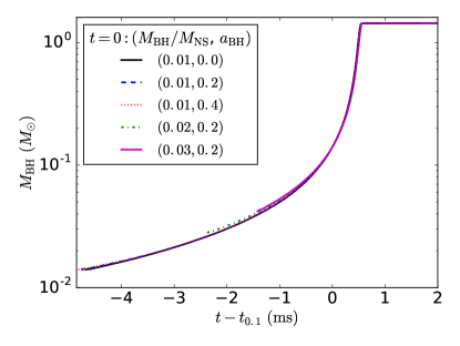
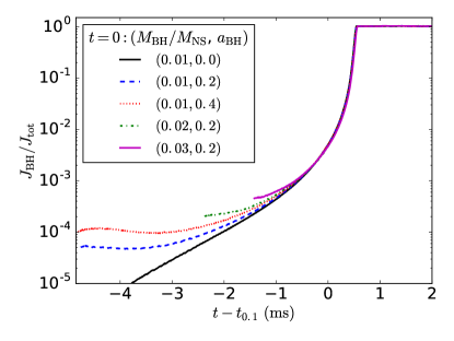
Figure 6: The mass (top) and angular momentum (bottom) of the BH as a function of time for cases with the ENG EOS and $a_{\rm NS}=0.4$, but different initial masses and spins for the BH. The curves have been aligned at the time where $M_{\rm BH}=0.1M_{\rm NS}$.

Another issue is what value should be chosen for $a_{\rm BH}$. For simplicity, we just set $a_{\rm BH}=a_{\rm NS}$. With this value, $a_{\rm BH}$ decreases during the BH’s initial growth, but as evident in the bottom panel of Fig. 6, the initial value of $a_{\rm BH}$ becomes unimportant by the time the BH doubles or triples in mass.

Appendix B Numerical convergence and comparison of axisymmetry to 3D

In axisymmetry, our numerical grid spans the half-plane $(x,z)\in[0,\infty)\times(-\infty,\infty)$. For our default resolution we use 13 levels of 2:1 mesh refinement with $257\times 129$ points on the coarsest level, and a resolution of $dx\approx 3\times 10^{-4}M_{\rm NS}$ on the finest level. The mesh refinement levels are dynamically adjusted according to truncation error estimates in the metric functions. The initial threshold is set so that the BH region is completely covered by the finest level during the first part of the evolution, and is only dropped after the BH doubles in size.

To establish convergence, and to estimate truncation error, we also perform simulations of the ENG EOS, $a_{\rm NS}=0.4$ case (with $M_{\rm BH}=0.01M_{\rm NS}$ and $a_{\rm BH}=a_{\rm NS}$) at 1.5 and $2\times$ higher resolution (i.e., with grid spacing that is $2/3$ and $1/2\times$ smaller). In Fig. 7, we demonstrate the convergence of the constraints. We show the evolution of the BH mass and spin for this resolution study in Fig. 8. The main effect of finite resolution is a slight overestimate of the BH accretion rate, and an underestimate of the BH spin.

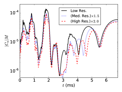
Figure 7: The convergence of the L2 norm of the generalized harmonic constraint violation $C_{a}=H_{a}-\Box x_{a}$ (average value in the $[-15M_{\rm NS},15M_{\rm NS}]\times[0,15M_{\rm NS}]$ central portion of the domain) for the case with the ENG EOS and $a_{\rm NS}=0.4$. The results have been scaled assuming first order convergence, though at early times the convergence in the quantity is close to second order.

We also simulate this same case in full 3D, i.e. without explicitly enforcing axisymmetry, in order to check whether there are any nonaxisymmetric instabilities. We use resolution equivalent to the default resolution used in axisymmetry. Because of the expense of evolving in full 3D, we begin the evolution when $M_{\rm BH}=0.05M_{\rm NS}$, using the axisymmetric evolution to determine the initial conditions. As also shown in Fig. 8, we find almost no difference in the growth of the BH.

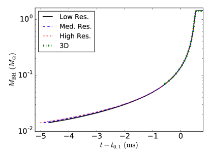
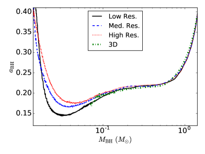
Figure 8: Top: The mass of the BH as a function of time for the case with the ENG EOS and $a_{\rm NS}=0.4$ for several different numerical resolutions. We also include the curve from a three-dimensional (i.e., without assuming axisymmetry) evolution of the final $\sim$ ms of the collapse that uses the axisymmetry evolution for initial data. The curves have been aligned at the time $t_{\rm 0.1}$ where $M_{\rm BH}=0.1M_{\rm NS}$. The primary effect of finite resolution is to decrease $t_{\rm 0.1}$, with the Richardson extrapolation (consistent with first order convergence) using all three resolutions giving $t_{\rm 0.1}\approx 5.4$ ms. Bottom: The dimensionless spin of the BH versus its mass for the same cases.

We also check for nonaxisymmetric modes by computing the azimuthal decomposition of the density:

$$C_{\rm m}=\int\rho_{0}u^{t}\sqrt{-g}e^{im\phi}d^{3}x$$ (4)

where $g$ is metric determinant, as was done in Refs. Paschalidis et al. (2015); East et al. (2016) in order to study the one-arm mode instability in hypermassive NSs. We plot $C_{m}$, for $m=1$ to 4, as a function of time in Fig. 9. The largest component is the $m=4$, which is expected from the truncation error associated with discretizing a sphere on a Cartesian grid, and all the modes remain negligible throughout. There is no evidence for any growing nonaxisymmetric modes before the time that the BH has consumed order unity of the NS’s mass.

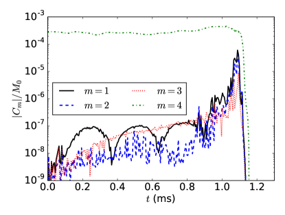
Figure 9: The nonaxisymmetric density modes, normalized by the total initial rest mass of the star, in the 3D simulation as a function of time. The sudden decrease at $t\approx 1.1$ ms corresponds to time when the NS is almost completely consumed by the BH.

Appendix C Estimates

To gain insight into the accretion process and the consequences for the dynamical behavior, it is convenient to visualize the NS-BH interaction in “shellular” terms. In particular, we further distinguish three distinct regions: (i) a BH with mass and spin parameters $M_{\rm BH}$, and $a_{\rm BH}$; (ii) an about to be accreted thin shell at radius $R_{s}\approx R_{\rm BH}$ with mass $\delta M_{s}$ and angular momentum $\delta J_{s}$ that is uniformly rotating with angular rotational velocity $\Omega_{s}$; and (iii) the rest of the star, with mass $M_{R}$, and angular velocity $\Omega_{R}(r)$. At the onset, the angular velocity is constant and set by the NS spin: $\Omega_{s}=\Omega_{R}(r)=\Omega_{\rm NS}$.

The shell being accreted by the BH induces a change of mass and angular momentum. The amount of the latter is constrained by the BH satisfying the Kerr bound $a_{\rm BH}\leq 1$ (we assume throughout this section that cosmic censorship holds). Let us analyze the change in the dimensionless BH spin due to accretion. From the definition of $a_{\rm BH}\equiv J_{\rm BH}/M_{\rm BH}^{2}$,

$$\delta a_{\rm BH}=M_{\rm BH}^{-2}\left(\delta J_{\rm BH}-2a_{\rm BH}M_{\rm BH}\delta M_{\rm BH}\right)\ .$$ (5)

Approximating the angular momentum of the shell using the Newtonian expression for a rotating spherical shell $\delta J_{s}=(2/3)\delta M_{s}R_{\rm BH}^{2}\Omega_{s}$, upon accretion of the whole shell the change in dimensionless BH spin is:

$$\delta a_{\rm BH}=\frac{\delta M_{s}}{M_{\rm BH}}\left(\frac{2}{3}\frac{R_{\rm BH}^{2}\Omega_{s}}{M_{\rm BH}}-2a_{\rm BH}\right)\ .$$ (6)

Since $R_{\rm BH}$ grows with $M_{\rm BH}$, for $\Omega_{s}\propto M_{\rm BH}^{p}$, it is clear that if $p\geq-1$, as the BH grows its spin will remain below the Kerr bound. With this observation, one can derive also what is expected for $\delta J/(\delta MR_{\rm BH})$ for the BH. Continuing with our Newtonian approximation, we can estimate the accretion of mass and angular momentum as a function of polar angle of a shell of width $\delta R$,

$$\frac{d\delta M}{d\theta} = R^{2}\delta R2\pi\sin\theta\rho\ ,$$ (7)

$$\frac{d\delta J}{d\theta} = (R^{2}\delta R2\pi\sin\theta\rho)R^{2}\sin^{2}\theta\Omega_{s}\ .$$ (8)

At constant $R$, these expressions imply $(d\delta J/d\theta)/(d\delta M/d\theta)\propto\sin^{2}\theta$ as observed in our simulations. If at any point the angular rotation $\Omega_{s}$ were to approach breakup, the assumption that the BH is accreting rigidly rotating spherical shells should break down, and the accretion of material near the equator would be strongly affected.

Several possible values for $p$ in the relation $\Omega_{s}\propto M_{\rm BH}^{p}$ are as follows:

1. $p=0$: The angular velocity of the accreted material remains constant at the initial value $\Omega_{\rm NS}$ set by NS spin. After the initial transient stage, this is not consistent with what is seen in the simulations.

2. $p=-1$: This would arise if the angular rotation at the accretion radius obeys a Keplerian relation $\Omega_{K}=\sqrt{M_{\rm BH}/R_{\rm BH}^{3}}$, or is given by the BH horizon rotational rate $\Omega_{H}=a_{\rm BH}/(2R_{\rm BH})$. This behavior is consistent with observations in the intermediate regime where the spin remains nearly constant.

3. $p=-4/3$: This would arise if every spherical shell fell from an initial radius $R_{i}\sim[3M_{\rm BH}/(4\pi\rho)]^{1/3}\propto M_{\rm BH}^{1/3}$ (assuming constant density) with its angular rotational velocity growing like $\Omega_{s}=\Omega_{\rm NS}(R_{i}/R_{\rm BH})^{2}$ to maintain constant angular momentum. As noted above, such a power would mean that $a_{\rm BH}$ would grow towards unity when the BH was sufficiently small. It would also mean that $\delta J/(\delta MR_{\rm BH})$ would decrease as the BH grows, which is not observed in the simulations.

We are thus left with the following picture. At early stages, the BH grows in mass and its spin parameter either decreases or increases as dictated by Eq. (6) depending on its initial value. Then, an intermediate stage takes place where the BH has roughly constant dimensionless spin, and grows keeping $\delta J/(\delta MR_{\rm BH})$ roughly constant. The rest of the star increases its angular rotation rate as the star is gradually consumed by the BH. Our simulations show $\Omega_{\rm BH}$ decreases during this stage as $R_{\rm BH}^{-1}$ while $\Omega(r=R_{s})$ (the rotational velocity of the star’s surface) increases. The dynamics induce a radial dependence on $\Omega(r)$, which we fit to an expression $\Omega=A+B/r^{n}$.

References

- Goldman and Nussinov (1989) I. Goldman and S. Nussinov, Phys. Rev. D40, 3221 (1989).
- de Lavallaz and Fairbairn (2010) A. de Lavallaz and M. Fairbairn, Phys. Rev. D81, 123521 (2010), arXiv:1004.0629 [astro-ph.GA] .
- Kouvaris and Tinyakov (2011) C. Kouvaris and P. Tinyakov, Phys. Rev. D83, 083512 (2011), arXiv:1012.2039 [astro-ph.HE] .
- McDermott et al. (2012) S. D. McDermott, H.-B. Yu, and K. M. Zurek, Phys. Rev. D85, 023519 (2012), arXiv:1103.5472 [hep-ph] .
- Bramante and Linden (2014) J. Bramante and T. Linden, Phys. Rev. Lett. 113, 191301 (2014), arXiv:1405.1031 [astro-ph.HE] .
- Bramante and Elahi (2015) J. Bramante and F. Elahi, Phys. Rev. D91, 115001 (2015), arXiv:1504.04019 [hep-ph] .
- Bramante et al. (2018) J. Bramante, T. Linden, and Y.-D. Tsai, Phys. Rev. D97, 055016 (2018), arXiv:1706.00001 [hep-ph] .
- Capela et al. (2013) F. Capela, M. Pshirkov, and P. Tinyakov, Phys. Rev. D87, 123524 (2013), arXiv:1301.4984 [astro-ph.CO] .
- Fuller and Ott (2015) J. Fuller and C. Ott, Mon. Not. Roy. Astron. Soc. 450, L71 (2015), arXiv:1412.6119 [astro-ph.HE] .
- Bramante and Linden (2016) J. Bramante and T. Linden, Astrophys. J. 826, 57 (2016), arXiv:1601.06784 [astro-ph.HE] .
- Fuller et al. (2017) G. M. Fuller, A. Kusenko, and V. Takhistov, Phys. Rev. Lett. 119, 061101 (2017), arXiv:1704.01129 [astro-ph.HE] .
- Abbott et al. (2017) B. P. Abbott et al. (Virgo, LIGO Scientific), Phys. Rev. Lett. 119, 161101 (2017), arXiv:1710.05832 [gr-qc] .
- Yang et al. (2018) H. Yang, W. E. East, and L. Lehner, Astrophys. J. 856, 110 (2018), [Erratum: Astrophys. J.870,no.2,139(2019)], arXiv:1710.05891 [gr-qc] .
- Hinderer et al. (2018) T. Hinderer et al., (2018), arXiv:1808.03836 [astro-ph.HE] .
- Foucart et al. (2019) F. Foucart, M. D. Duez, L. E. Kidder, S. Nissanke, H. P. Pfeiffer, and M. A. Scheel, Phys. Rev. D99, 103025 (2019), arXiv:1903.09166 [astro-ph.HE] .
- Siegel (2019) D. M. Siegel, (2019), arXiv:1901.09044 [astro-ph.HE] .
- Kouvaris and Tinyakov (2014) C. Kouvaris and P. Tinyakov, Phys. Rev. D90, 043512 (2014), arXiv:1312.3764 [astro-ph.SR] .
- Markovic (1995) D. Markovic, Mon. Not. Roy. Astron. Soc. 277, 25 (1995).
- Stergioulas and Friedman (1995) N. Stergioulas and J. Friedman, Astrophys. J. 444, 306 (1995), arXiv:astro-ph/9411032 [astro-ph] .
- East et al. (2012a) W. E. East, F. M. Ramazanoglu, and F. Pretorius, Phys.Rev. D86, 104053 (2012a), arXiv:1208.3473 [gr-qc] .
- East et al. (2012b) W. E. East, F. Pretorius, and B. C. Stephens, Phys.Rev. D85, 124010 (2012b), arXiv:1112.3094 [gr-qc] .
- Berger and Colella (1989) M. Berger and P. Colella, Journal of Computational Physics 82, 64 (1989).
- Abbott et al. (2018) B. P. Abbott et al. (Virgo, LIGO Scientific), Phys. Rev. Lett. 121, 161101 (2018), arXiv:1805.11581 [gr-qc] .
- Read et al. (2009) J. S. Read, B. D. Lackey, B. J. Owen, and J. L. Friedman, Phys. Rev. D79, 124032 (2009), arXiv:0812.2163 [astro-ph] .
- Bauswein et al. (2010) A. Bauswein, H.-T. Janka, and R. Oechslin, Phys. Rev. D 82, 084043 (2010).
- Landau and Lifshitz (1987) L. D. Landau and E. M. Lifshitz, Fluid Mechanics. Second Edition. 1987. Pergamon, Oxford (1987).
- Camelio et al. (2018) G. Camelio, T. Dietrich, and S. Rosswog, Mon. Not. Roy. Astron. Soc. 480, 5272 (2018), arXiv:1806.07775 [astro-ph.HE] .
- Duez et al. (2006) M. D. Duez, Y. T. Liu, S. L. Shapiro, M. Shibata, and B. C. Stephens, Phys. Rev. Lett. 96, 031101 (2006), arXiv:astro-ph/0510653 [astro-ph] .
- Baiotti et al. (2007) L. Baiotti, I. Hawke, and L. Rezzolla, New frontiers in numerical relativity. Proceedings, International Meeting, NFNR 2006, Potsdam, Germany, July 17-21, 2006, Class. Quant. Grav. 24, S187 (2007), arXiv:gr-qc/0701043 [gr-qc] .
- Giacomazzo et al. (2011) B. Giacomazzo, L. Rezzolla, and N. Stergioulas, Phys. Rev. D84, 024022 (2011), arXiv:1105.0122 [gr-qc] .
- Lehner et al. (2012) L. Lehner, C. Palenzuela, S. L. Liebling, C. Thompson, and C. Hanna, Phys. Rev. D86, 104035 (2012), arXiv:1112.2622 [astro-ph.HE] .
- Falcke and Rezzolla (2014) H. Falcke and L. Rezzolla, Astron. Astrophys. 562, A137 (2014), arXiv:1307.1409 [astro-ph.HE] .
- Proudman (1956) I. Proudman, Journal of Fluid Mechanics 1, 505–516 (1956).
- Martynov et al. (2019) D. Martynov et al., Phys. Rev. D99, 102004 (2019), arXiv:1901.03885 [astro-ph.IM] .
- Amiri et al. (2019) M. Amiri et al. (CHIME/FRB), Nature 566, 230 (2019), arXiv:1901.04524 [astro-ph.HE] .
- Newburgh et al. (2016) L. B. Newburgh et al., Proceedings, Ground-based and Airborne Telescopes VI: Edinburgh, United Kingdom, June 26-July 1, 2016, Proc. SPIE Int. Soc. Opt. Eng. 9906, 99065X (2016), arXiv:1607.02059 [astro-ph.IM] .
- Carilli and Rawlings (2004) C. L. Carilli and S. Rawlings, International SKA Conference 2003 Geraldton, Australia, July 27-August 2, 2003, New Astron. Rev. 48, 979 (2004), arXiv:astro-ph/0409274 [astro-ph] .
- Nan et al. (2011) R. Nan, D. Li, C. Jin, Q. Wang, L. Zhu, W. Zhu, H. Zhang, Y. Yue, and L. Qian, Int. J. Mod. Phys. D20, 989 (2011), arXiv:1105.3794 [astro-ph.IM] .
- Goldstein et al. (2017) A. Goldstein, P. Veres, E. Burns, M. S. Briggs, R. Hamburg, D. Kocevski, C. A. Wilson-Hodge, R. D. Preece, S. Poolakkil, O. J. Roberts, C. M. Hui, V. Connaughton, J. Racusin, A. von Kienlin, T. Dal Canton, N. Christensen, T. Littenberg, K. Siellez, L. Blackburn, J. Broida, E. Bissaldi, W. H. Cleveland, M. H. Gibby, M. M. Giles, R. M. Kippen, S. McBreen, J. McEnery, C. A. Meegan, W. S. Paciesas, and M. Stanbro, Astrophys. J. Letters 848, L14 (2017), arXiv:1710.05446 [astro-ph.HE] .
- Albert et al. (2018) A. Albert et al. (HAWC), JCAP 1806, 043 (2018), [Erratum: JCAP1904,no.04,E01(2019)], arXiv:1804.00628 [astro-ph.HE] .
- Abeysekara et al. (2018) A. U. Abeysekara et al. (VERITAS, Fermi-LAT, HAWC), Astrophys. J. 866, 24 (2018), arXiv:1808.10423 [astro-ph.HE] .
- Archer et al. (2019) A. Archer et al., Astrophys. J. 876, 95 (2019), arXiv:1904.09329 [astro-ph.HE] .
- Paschalidis et al. (2015) V. Paschalidis, W. E. East, F. Pretorius, and S. L. Shapiro, Phys. Rev. D92, 121502 (2015), arXiv:1510.03432 [astro-ph.HE] .
- East et al. (2016) W. E. East, V. Paschalidis, F. Pretorius, and S. L. Shapiro, Phys. Rev. D93, 024011 (2016), arXiv:1511.01093 [astro-ph.HE] .