Abstract

We have performed 3D numerical simulations for merger of equal mass binary neutron stars in full general relativity. We adopt a $\Gamma$-law equation of state in the form $P=(\Gamma-1)\rho\varepsilon$ where $P$, $\rho$, $\varepsilon$ and $\Gamma$ are the pressure, rest mass density, specific internal energy, and the adiabatic constant with $\Gamma=2$. As initial conditions, we adopt models of corotational and irrotational binary neutron stars in a quasi-equilibrium state which are obtained using the conformal flatness approximation for the three geometry as well as an assumption that a helicoidal Killing vector exists. In this paper, we pay particular attention to the final product of the coalescence. We find that the final product depends sensitively on the initial compactness parameter of the neutron stars : In a merger between sufficiently compact neutron stars, a black hole is formed in a dynamical timescale. As the compactness is decreased, the formation timescale becomes longer and longer. It is also found that a differentially rotating massive neutron star is formed instead of a black hole for less compact binary cases, in which the rest mass of each star is less than $70-80\%$ of the maximum allowed mass of a spherical star. In the case of black hole formation, we roughly evaluate the mass of the disk around the black hole. For the merger of corotational binaries, a disk of mass $\sim 0.05-0.1M_{*}$ may be formed, where $M_{*}$ is the total rest mass of the system. On the other hand, for the merger of irrotational binaries, the disk mass appears to be very small : $<0.01M_{*}$.

[

]

I Introduction

Several neutron star-neutron star binaries are known to exist in our galaxy [1]. According to high precision measurements of the general relativistic (GR) effects on their orbital motion, three of these binaries are going to merge as a result of gravitational radiation reaction within the Hubble timescale $\sim 10^{10}$ years. What are the final fates of these binaries after the mergers? Their total gravitational masses are is in a narrow range $\sim 2.65-2.85M_{\odot}$ where $M_{\odot}$ denotes the solar mass. The stars will not be tidally disrupted before the merger, since the masses of the two stars in each binary are nearly equal. Hence, the mass loss from the binary systems is expected to be small during their evolution and the mass of the merged object will be approximately equal to the initial mass. The maximum allowed gravitational mass for spherical neutron stars is in a range $\sim 1.5-2.3M_{\odot}$ depending on the nuclear equation of state [2, 3]. Even if we take into account the effect of rigid rotation, it is increased by at most $\sim 20\%$ [4]. Judging from these facts, the compact objects formed just after the merger of these binary systems seem bound to collapse to a black hole.

However, this is not the case if the merged object rotates differentially. The maximum allowed mass can be increased by a larger factor ($>50\%$) due to the differential rotation [5], which suggests that the merged objects of $\sim 2.5-3M_{\odot}$ may be dynamically stable against gravitational collapse to a black hole. Such differentially rotating stars could be secularly unstable, since viscosity or magnetic field could change the differential rotation into rigid rotation. A star with a high ratio of rotational energy to the gravitational binding energy could also be secularly unstable to gravitational wave emission [6]. These processes might dissipate or redistribute the angular momentum, and induce eventual gravitational collapse to a black hole. However, the timescales for such secular instabilities are in general much longer than the dynamical timescale of the system. Hence, the merged objects may not collapse to a black hole promptly, but remain as a massive neutron star supported by differential rotation at least for these secular timescales. These facts imply that the final product of the merger of binary neutron stars is an open question depending not only on the nuclear equation of state for high density neutron matter but also on the rotational profile of the merged object.

Interest in the final product of binary coalescence has been stimulated by the prospect of future observation of extragalactic binary neutron stars by gravitational wave detectors. A statistical study shows that mergers of binary neutron stars may occur at a few events per year within a distance of a few hundred Mpc [7]. This suggests that binary merger is a promising source of gravitational waves. Although the frequency of gravitational waves in the merging regime will be larger than $1$kHz and lies beyond the upper end of the frequency range accessible to laser interferometers such as LIGO [8] for a typical event at a distance $\sim 200$Mpc, it may be observed using specially designed narrow band interferometers or resonant-mass detectors [9]. Such future observations will provide valuable information about the merger mechanism of binary neutron stars and the final products.

Interest has also been stimulated by a hypothesis about the central engine of $\gamma$-ray bursts (GRBs) [10]. Recently, some of GRBs have been shown to be of cosmological origin [11]. In cosmological GRBs, the central sources must supply a large amount of the energy $\gtrsim 10^{51}$ ergs in a very short timescale of order from a millisecond to a second. It has been suggested that the merger of binary neutron stars is a likely candidate for the powerful central source [10]. In the typical hypothetical scenario, the final product should be a system composed of a rotating black hole surrounded by a massive disk of mass $>0.1M_{\odot}$, which could supply the large amount of energy by neutrino processes or by extracting the rotational energy of the black hole.

To investigate the final product of the merger theoretically, numerical simulation appears to be the unique promising approach. Considerable effort has been made for this in the framework of Newtonian and post-Newtonian gravity [12, 13, 14, 15, 16, 17]. Although these simulations have clarified a wide variety of physical features which are important during the coalescence of binary neutron stars, a fully GR treatment is obviously necessary for determining the final product because GR effects are crucial.

Intense efforts have been made for constructing a reliable code for 3D hydrodynamic simulation in full general relativity in the past decade [18, 19, 20, 21]. Recently, Shibata presented a wide variety of numerical results of test problems for his fully GR code and showed that simulations for many interesting problems are now feasible [21].

To perform a realistic simulation, we also need realistic initial conditions for the merger, i.e., a realistic density distribution and velocity field for the component stars. Since the timescale of gravitational wave emission is longer than the orbital period, we may consider the binary neutron stars to be in a quasi-equilibrium state even just before the merger. The velocity field in the neutron stars has been turned out to be nearly irrotational because (1) the shear viscosity is too small to redistribute angular momentum to produce a corotational velocity field during the timescale of gravitational wave emission and (2) the initial vorticity of each star is negligible as long as the rotational period of the neutron stars is not $\sim$ milliseconds [22]. Therefore, as realistic initial conditions, we should prepare a quasi-equilibrium state of binary neutron stars with an irrotational velocity field. Recently, several groups have developed various numerical methods to compute GR irrotational binary neutron stars in quasi-equilibrium in a framework with the appropriate approximations that a helicoidal Killing vector (see Eq. (20) for definition) exists and that the three geometry is conformally flat [23, 24, 25]. Their numerical results have been compared and found to agree to within a few percent error in the gravitational mass and the central density as a function of orbital separation.

In this paper, we perform simulations for the merger of binary neutron stars of equal mass by using these new numerical implementations developed recently. As a first step, we adopt a simple $\Gamma$-law equation of state with $\Gamma=2$ as a reasonable qualitative approximation to the high density nuclear equation of state. Although microscopic effects such as cooling due to neutrino emission or heating due to bulk viscosity may become important for discussing the merging process in detail [16], we neglect them here for simplicity. The purpose of this paper is to investigate the dynamical nature of the mergers, the final products after the mergers and the dependence of these outcomes on the initial velocity field and the compactness parameter of the binary neutron stars. Simulations are performed not only for irrotational binaries but also for corotational ones to clarify the difference due to the initial velocity field.

Throughout this paper, we adopt the units $G=c=M_{\odot}=1$ where $G$ and $c$ denote the gravitational constant and speed of light, respectively. Latin and Greek indices denote spatial components ($1-3$) and space-time components ($0-3$), respectively. $\delta_{ij}(=\delta^{ij})$ denotes the Kronecker delta. We use Cartesian coordinates $x^{k}=(x,y,z)$ as the spatial coordinates with $r=\sqrt{x^{2}+y^{2}+z^{2}}$; $t$ denotes coordinate time.

II Methods

A Summary of formulation

We have performed numerical simulations using the same formulation as in [21], to which the reader may refer for details about the basic equations, the gauge conditions and the computational method. The fundamental variables used in this paper are:

$$\rho :{\rm rest~{}mass~{}density},$$ (1)

$$\varepsilon :{\rm specific~{}internal~{}energy},$$ (2)

$$P :{\rm pressure},$$ (3)

$$u^{\mu} :{\rm four~{}velocity},$$ (4)

$$v^{i} ={u^{i}\over u^{0}},$$ (5)

$$\alpha :{\rm lapse~{}function},$$ (6)

$$\beta^{k} :{\rm shift~{}vector},$$ (7)

$$\gamma_{ij} :{\rm metric~{}in~{}3D~{}spatial~{}hypersurface},$$ (8)

$$\gamma ={\rm det}(\gamma_{ij})=e^{12\phi}=\psi^{12},$$ (9)

$$\tilde{\gamma}_{ij} =e^{-4\phi}\gamma_{ij},$$ (10)

$$K_{ij} :{\rm extrinsic~{}curvature}.$$ (11)

These variables (together with auxiliary functions $F_{i}$ and the trace of the extrinsic curvature $K_{k}^{~{}k}$) are numerically evolved as an initial value problem (see [26, 27] for details of the numerical method for handling the evolution equations and initial value equations). Several test calculations, including spherical collapse of dust, stability of spherical neutron stars, and the evolution of rotating neutron stars as well as corotational binary systems have been presented in [21]. Violations of the Hamiltonian constraint [28] and conservation of rest mass and angular momentum [29] are monitored to check the accuracy, and we stop simulations before the accuracy becomes too poor. Black holes which are formed during the last phase of the merger are located with an apparent horizon finder described in [30].

We also define a density $\rho_{*}(=\rho\alpha u^{0}e^{6\phi})$ from which the total rest mass of the system can be integrated as

$$M_{*}=\int d^{3}x\rho_{*}.$$ (12)

We have performed the simulations using a fixed uniform grid with a typical size of $233\times 233\times 117$ for the $x-y-z$ directions, respectively, and assuming reflection symmetry with respect to the $z=0$ plane. All of the results shown in Sec. IV are obtained from simulations with this grid size. We have also performed a number of test simulations with a smaller grid size of $193\times 193\times 97$ changing the grid spacing and location of the outer boundaries to confirm that the results do not change significantly. For one model (I2) (see Sec. III and Table I), we performed a simulation with a larger grid size of $293\times 293\times 147$, widening the computational domain to investigate the effect of the outer boundary on the gravitational waveforms.

The slicing and spatial gauge conditions which we use in this paper are basically the same as those adopted in [26, 27, 21]; i.e., we impose an “approximate” maximal slicing condition ($K_{k}^{~{}k}\simeq 0$) and an “approximate” minimum distortion gauge condition ($\tilde{D}_{i}(\partial_{t}\tilde{\gamma}^{ij})\simeq 0$ where $\tilde{D}_{i}$ is the covariant derivative with respect to $\tilde{\gamma}_{ij}$). However, for the cases when a merged object collapses to form a black hole, we slightly modify the spatial gauge condition in order to improve the spatial resolution around the black hole forming region. The method of the modification is described in Sec. II.B.

Throughout this paper, we assume a $\Gamma$-law equation of state in the form

$$P=(\Gamma-1)\rho\varepsilon,$$ (13)

where $\Gamma$ is the adiabatic constant. For the hydrostatic problem, which appears in solving for initial value configurations, the equation of state can be rewritten in the polytropic form

$$P=K\rho^{\Gamma},\mbox{~{}~{}~{}~{}~{}}\Gamma=1+\frac{1}{n},$$ (14)

where $K$ is a constant (different from $K_{k}^{~{}k}$) and $n$ is the polytropic index. We adopt $\Gamma=2$ ($n=1$) as a qualitative approximation to realistic, moderately stiff equations of state for neutron stars.

Physical units enter only through the constant $K$, which can be chosen arbitrarily or completely scaled out of the problem. In the following, we quote values for $K=200/\pi$, for which in our units ($G=c=M_{\odot}=1$) the radius of a spherical star is $R=(\pi K/2)^{1/2}=10(\sim 15{\rm km})$ in the Newtonian limit. Since $K^{n/2}$ has units of length, dimensionless variables can be constructed as

$$\bar{M}_{*}=M_{*}K^{-n/2}, \bar{M}_{g}=M_{g}K^{-n/2}, \bar{R}=RK^{-n/2},$$ (15)

$$\bar{J}=JK^{-n}, \bar{P}_{\rm orb}=P_{\rm orb}K^{-n/2}, \bar{\rho}=\rho K^{n},$$ (16)

where $M_{g}$, $J$ and $P_{\rm orb}$ denote the gravitational mass, angular momentum and orbital period. All results can be rescaled for arbitrary $K$ using Eqs. (15). (For example, the maximum value of $M_{*}$ for spherical stars is $1.435M_{\odot}$ for $K=200/\pi(G^{3}M_{\odot}^{2}/c^{4})$ with the rest mass density $\simeq 3.1\times 10^{15}{\rm g/cm}^{3}$. If we want to choose $M_{*}$ as $2M_{\odot}$, we should change $K$ to $123.7(G^{3}M_{\odot}^{2}/c^{4})$ and the corresponding density is then $\simeq 1.6\times 10^{15}{\rm g/cm}^{3}$; cf. Fig. 1. ) In other words, the invariant quantities are only the dimensionless quantities such as $M_{*}/M_{g}$, $M_{g}/R$, $M_{g}/P_{\rm orb}$ and $J/M_{g}^{2}$.

B Spatial gauge condition

When a black hole is not formed as a final product of the merger, we adopt the approximate minimum distortion gauge condition as our spatial gauge condition (henceforth referred to as the AMD gauge condition). However, as pointed out in previous papers [21, 27], during black hole formation (i.e., for an infalling radial velocity field), the expansion of the shift vector $\partial_{i}\beta^{i}$ and $\partial_{t}\phi\simeq\partial_{i}\beta^{i}/6$ become positive using this gauge condition together with our slicing $K_{k}^{~{}k}\simeq 0$. Accordingly, the coordinates diverge outwards and the resolution around the black hole forming region becomes worse and worse during the collapse. This undesirable property motivates us to modify the AMD gauge condition when we treat black hole formation. Following [27], we modify the AMD shift vector as

$$\beta^{i}=\beta^{i}_{\rm AMD}-f(t,r){x^{i}\over r+\epsilon}\beta^{r^{\prime}}_{\rm AMD}.$$ (17)

Here $\beta^{i}_{\rm AMD}$ denotes the shift vector for the AMD gauge condition, $\beta^{r^{\prime}}_{\rm AMD}\equiv x^{k}\beta^{k}_{\rm AMD}/(r+\epsilon)$, $\epsilon$ is a small constant much smaller than the grid spacing, and $f(t,r)$ is a function chosen specifically as

$$f(t,r)=f_{0}(t){1\over 1+(r/3M_{g0})^{6}}.$$ (18)

where $M_{g0}$ denotes the gravitational mass of a system at $t=0$. We determine $f_{0}(t)$ from $\phi_{0}=\phi(r=0)$. Taking into account the fact that the resolution around $r=0$ deteriorates when $\phi_{0}$ becomes large, we choose $f_{0}$ as

$$f_{0}(t)=\left\{\begin{array}[]{ll}\displaystyle 1&{\rm for}~{}\phi_{0}\geq 0.8,\\ 2.5\phi_{0}-1&{\rm for}~{}0.4\leq\phi_{0}\leq 0.8,\\ 0&{\rm for}~{}\phi_{0}<0.4,\\ \end{array}\right.$$ (19)

Note that for spherical collapse with $f_{0}=1$, $\partial_{i}\beta^{i}\simeq 0$ and $\partial_{t}\phi\simeq 0$ at $r=0$. We employ this modified gauge condition whenever a merged object collapses to form a black hole.

It is worth mentioning that with this modification, the coordinate radius of the apparent horizon (when it is formed) becomes larger than without the modification. This implies that more grid points are located along the radius of the apparent horizon and accuracy for determination of the apparent horizon is improved.

III Initial conditions

Even just before the merger, the binary neutron stars are considered to be in a quasi-equilibrium state because the timescale of gravitational radiation reaction $\sim 5/\{64\Omega(M_{g}\Omega)^{5/3}\}$ [2], where $\Omega$ denotes the orbital angular velocity of the binary neutron stars, is several times longer than the orbital period. Thus, for performing a realistic simulation of the merger, we should prepare a quasi-equilibrium state as the initial condition. In this paper, we construct such initial conditions as follows.

First, we assume the existence of a helicoidal Killing vector

$$\ell^{\mu}=(1,-y\Omega,x\Omega,0).$$ (20)

Since emission of gravitational waves violates the helicoidal symmetry, this assumption does not strictly hold in reality. However, as mentioned above, the emission timescale of gravitational waves is several times longer than the orbital period even just before the merger (cf. Table I) so that this assumption can be acceptable for obtaining an approximate quasi-equilibrium state. In addition to this assumption, we adopt the so-called conformal flatness approximation in which the three geometry is assumed to be conformally flat, for simplicity.

In this paper, we consider irrotational and corotational binary neutron stars. Then, the geometric [33] and hydrostatic equations [34] for solutions of the quasi-equilibrium states are described as

$$\Delta\psi=-2\pi(\rho hw^{2}-K\rho^{\Gamma})\psi^{5}-{\psi^{5}\over 8}\delta^{ik}\delta^{jl}L_{ij}L_{kl},$$ (21)

$$\Delta(\alpha\psi)=2\pi\alpha\psi^{5}[\rho h(3w^{2}-2)+5K\rho^{\Gamma}]$$ (22)

$$\hskip 42.67912pt+{7\alpha\psi^{5}\over 8}\delta^{ik}\delta^{jl}L_{ij}L_{kl},$$ (23)

$$\delta_{ij}\Delta\beta^{i}+{1\over 3}\beta^{k}_{~{},kj}-2L_{jk}\delta^{ki}\Bigl{(}\partial_{i}\alpha-{6\alpha\over\psi}\partial_{i}\psi\Bigr{)}$$ (24)

$$\hskip 85.35826pt=16\pi\alpha\rho hwu_{j},$$ (25)

$${\alpha h\over w}+hu_{k}V^{k}={\rm const.},$$ (26)

where

$$w=\alpha u^{0}=\sqrt{1+\psi^{-4}\delta^{ij}u_{i}u_{j}},$$ (27)

$$h=1+K\Gamma\rho^{\Gamma-1}/(\Gamma-1),$$ (28)

$$L_{ij}={1\over 2\alpha}\biggl{(}\delta_{jk}\partial_{i}\beta^{k}+\delta_{ik}\partial_{j}\beta^{k}-{2\over 3}\delta_{ij}\partial_{k}\beta^{k}\biggr{)},$$ (29)

$$V^{k}=-\beta^{k}+\delta^{kl}{\alpha u_{l}\over w\psi^{4}}-\ell^{k}.$$ (30)

and $\Delta$ denotes the flat Laplacian in the three space. Eqs. (21–25) are the geometric equations and Eq. (26) is the so-called Bernoulli equation. $V^{k}$ can be regarded as the coordinate three velocity in the corotating frame rotating with angular velocity $\Omega$.

In the case of corotational binaries in which $V^{k}=0$, $u_{i}$ is written as

$$u_{i}=w\psi^{4}(\epsilon_{izk}\Omega x^{k}+\delta_{ij}\beta^{j})/\alpha.$$ (31)

In the case of irrotational binaries, on the other hand, $u_{i}$ is written as

$$u_{i}=h^{-1}\partial_{i}\Phi$$ (32)

where $\Phi$ denotes the velocity potential which satisfies an elliptic PDE [34]

$$\delta^{ij}\partial_{i}(\rho\alpha\psi^{2}h^{-1}\partial_{j}\Phi)-\partial_{i}[\rho\alpha h^{-1}\psi^{6}(\ell^{i}+\beta^{i})]=0,$$ (33)

with the following boundary condition at the stellar surface;

$$\left.V^{i}\partial_{i}\rho\right|_{\rm surf}=0.$$ (34)

The above Poisson type equations such as Eqs. (21–26) and (3.12) as well as the Bernoulli equation (26) are solved iteratively with appropriate boundary conditions. Corotational binaries are calculated using the same numerical method as adopted in [21]. Irrotational binaries are calculated using the method developed recently by Uryū and Eriguchi ([24], to which the reader may refer for details).

For the corotational case, we prepare binaries with several compactness parameters, with the surfaces of the two stars coming into contact. As shown in [33], such binaries with $\Gamma=2$ are located near to the energy minimum along the sequence of corotational binaries of constant rest mass. Therefore, they are expected to be located near to a marginally stable point for hydrodynamic [14] or GR orbital instability.

For the irrotational case, the sequence of binaries of constant rest mass ends when cusps (i.e., Lagrange (L1) points) appear at the inner edge of the stars [23, 24]. This is the case for any compactness parameter. If the stars in the binary system approach further, mass transfer will begin and the resulting state is not clear. As shown in [23], the closest binaries with cusps are far outside the energy minimum for $\Gamma=2$, which indicates that they are stable against hydrodynamic and GR orbital instability. Furthermore, the gravitational radiation reaction timescale is several times longer than the orbital period (cf. Table I). Thus, if we choose such a binary as the initial condition for a simulation, a few orbits are maintained stably before the merger starts, decreasing the orbital separation and changing the shapes in a quasi-adiabatic manner.

It is still difficult to perform an accurate simulation for such a quasi-adiabatic phase. It is desirable to choose a binary state which is located near to the unstable point against hydrodynamic or GR orbital instability and starts merging soon; i.e., a state after the nearly adiabatic phase. However, a method for obtaining such a state has not yet been developed. Hence, in this paper, we prepare the following initial conditions modifying the quasi-equilibrium state slightly. First, we prepare a binary in which cusps appear at the surfaces. Then, we reduce the angular momentum by $\simeq 2.5\%$ from the quasi-equilibrium state to destabilize the orbit and to induce the merger promptly [32]. We deduce that such an initial condition can be acceptable for the investigation of the final products after the merger since the decrease factor is still small. We performed test simulations changing the decrease factor slightly in the range $2-3\%$, and we indeed found that the results shown in Sec. IV are only weakly dependent on this parameter.

In the numerical computation of the quasi-equilibrium states as initial conditions, we typically adopt a grid spacing in which the major diameter of each star is covered by $\sim 35$ grid points. With this resolution, the error for the estimation of $M_{g}$ and $J$ is less than $1\%$ (e.g., [24]), and the gravitational radius of the system defined as $GM_{g0}/c^{2}$ is covered with $\sim 4-7$ grid points (cf. Table I). Keeping this grid spacing, the outer boundaries of the computational domain in the simulation are located at $\lesssim 0.3\lambda_{\rm gw}$ with $233\times 233\times 117$ grid points, where $\lambda_{\rm gw}(\equiv\pi/\Omega)$ denotes the characteristic wavelength of gravitational waves emitted from the binaries in a quasi-equilibrium state. With this setting, gravitational waveforms are not accurately evaluated because the outer boundaries are not located in the wave zone. In this paper, we pay particular attention to the merger process, final products, and dependence of these outcomes on initial parameters of the binaries, but we do not treat the accurate extraction of gravitational waveforms and hence the accurate computation of gravitational radiation back reaction. As mentioned above, we start with binaries in almost dynamically unstable orbits. This implies that the effect of radiation reaction is not very important in the early phase of the merger. In the later phase of the merger, the dynamical timescale seems to be shorter than the emission timescale of gravitational waves and the evolution of the merged object due to gravitational radiation is secular. Hence, we deduce that the effect due to the error in evaluating the radiation reaction is small throughout the evolution.

In Fig. 1, we show the relation between the rest mass $M_{*}$ and the maximum density $\rho_{\rm max}$ of each star for binaries in quasi-equilibrium states. The solid line denotes the relations for spherical neutron stars. The crosses and filled circles denote those for the corotational and irrotational binary neutron stars, respectively. The binaries which are used in the following simulation as initial conditions are marked with (C1), (C2), (C3), (I1), (I2) and (I3) (C and I denote “corotational” and “irrotational”, respectively). The relevant quantities for these initial conditions are shown in Table I. We note that the orbital period is calculated as

$$P_{\rm orb}=1.5{\rm msec}\biggl{(}{C_{i}\over 0.15}\biggr{)}^{-3/2}\biggl{(}{M_{g0}\over 2.8M_{\odot}}\biggr{)}.$$ (35)

In a realistic situation, each star of the binary has a small approaching velocity because of gravitational radiation reaction. We approximately add this to the above quasi-equilibrium state in setting the initial conditions. According to the quadrupole formula with Newtonian equations of motion, the absolute value of the approaching velocity of each star is written as [2]

$$v_{\rm a}=1.6(M_{g0}\Omega)^{2}.$$ (36)

Thus, in giving initial conditions, we change $u_{i}$ to be

$$u_{x}=(u_{x})_{\rm eq}-v_{\rm a}{|x|\over x},$$ (37)

where $(u_{x})_{\rm eq}$ denotes $u_{x}$ of the quasi-equilibrium state. Here, we implicitly assume that the center of mass of each star is initially located on the $x$-axis (see Figs. 2–4 and 9–11).

For models (C1), (C2) and (C3), we performed simulations without the approaching velocity and found that the outcomes such as the final products and the disk mass depend only weakly on this approaching velocity. Thus, it does not seem to affect the following results significantly.

IV Numerical results

A corotational cases

In Figs. 2–4, we show snapshots of the density contour lines for $\rho_{*}$ and velocity field $(v^{x},v^{y})$ in the equatorial plane at selected times for models (C1), (C2), and (C3), respectively. For (C1), a new massive neutron star is formed, while for other cases, a black hole is formed. We note that for model (C2), we could not determine the location of the apparent horizon before the simulation crashed, because the grid spacing was too wide to satisfactorily resolve the black hole forming region. However, the central value of the lapse function is small enough $<0.01$ at the crash so that we may judge that a black hole is formed in this simulation. On the other hand, for model (C3), we can determine the location of the apparent horizon (see the thick solid line in the last snapshot of Fig. 4).

Irrespective of the compactness parameters, the orbital distance gradually decreases due to the initial approach velocity. When it becomes small enough to destabilize the orbit due to the hydrodynamic or GR orbital instability, the orbital distance begins to quickly decrease and in the outer part, spiral arms are formed. For more compact binaries, the decrease rate of the orbital separation is larger because the initial approach velocity is larger, and the orbit soon becomes unstable. We deduce that the neutron stars for model (C3) are initially located near to the innermost stable circular orbit against GR orbital instability because their initial compactness $C_{i}\equiv(M_{g0}\Omega)^{2/3}\sim M_{g0}/a$, where $a$ denotes the orbital separation, is nearly equal to 1/6 (see Table I). Indeed, they begin merging soon after the simulation is started. Once merger begins, the spiral arms continue to develop transporting angular momentum outward in the outer part of the merged object.

For model (C1), the inner part first contracts after the orbit becomes unstable, but subsequently it bounces due to the pressure and centrifugal force. The shape of the merged object changes from ellipsoidal to spheroidal, redistributing the angular momentum as well as dissipating it by gravitational radiation. Eventually, it forms a new rapidly rotating neutron star. In Figs. 5 and 6, we show the density contour lines for $\rho_{*}$ in the $x-z$ plane and the angular velocity $\Omega\equiv(xv^{y}-yv^{x})/(x^{2}+y^{2})$ along the $x$ and $y$-axes in the equatorial plane at $t=2.07P_{\rm orb}$. It is found that the new neutron star is highly flattened and differentially rotating [31]. Note that the mass inside $r\simeq 7.5M_{g0}$ which appears to constitute the merged object is $\sim 0.97M_{*}(\simeq 2.16)$. Since the maximum allowed mass of a spherical star with $K=200/\pi$ is $M_{*~{}\rm max}^{\rm sph}\simeq 1.435$, the mass of the new neutron star is $\sim 50\%$ larger than this [35]. We point out that we have monitored the evolution of $K^{\prime}(x^{\mu})\equiv P/\rho^{\Gamma}$ which is initially equal to $K$ anywhere in the star and can be regarded as a measure of the entropy distribution. Since shock heating is not very effective in the merging, we have found that the value of $K^{\prime}$ increases by at most $\sim 10\%$ in the regions of high density. (Note that in the low density regions such as near to the surface of the merged object, $K^{\prime}$ is slightly larger.) Thus, the role of thermal energy increase is not significant for supporting the large mass in contrast with the case of head-on collision [36, 20]. The effect of differential rotation is important in the present case.

We note that the new rotating neutron star has a non-axisymmetric structure at the time when we stopped the simulation. Therefore it will evolve further as a result of gravitational wave emission, and may become unstable against gravitational collapse to become a black hole after a substantial amount of angular momentum is carried away [37].

For models (C2) and (C3), after the orbit becomes unstable, the inner part contracts due to self-gravity without bouncing because the pressure and centrifugal force are not strong enough to balance the self-gravity. Subsequently it collapses to form a black hole. Since the compactness is sufficiently large for model (C3), the inner part quickly collapses to form a black hole without a significant bounce. On the other hand, in the case of model (C2), the formation timescale of the black hole is longer because the compactness is smaller.

To show the features of the collapse around the central region, we show $\alpha$ at $r=0$ as a function of $t/P_{\rm orb}$ in Fig. 7. For model (C3), $\alpha(r=0)$ quickly approaches to zero, but for model (C2), the decrease rate becomes small at $t\sim 1.2P_{\rm orb}$. This difference indicates that the collapse is decelerated by the pressure and/or centrifugal force.

We note that for model (C2), the initial value of $J/M_{g}^{2}$ is larger than unity. Nevertheless, a black hole appears to be formed after the merger. This indicates that some mechanisms for angular momentum transfer or dissipation act to decrease $J/M_{g}^{2}$ to less than unity during the merger. We can expect that the following two mechanisms are effective. (a) In the case of corotational binaries, the outer part has a large amount of the angular momentum and spreads outwards forming the spiral arms. As a result, the specific angular momentum in the inner part which finally forms a black hole is smaller than that of the outer part and $J/M_{g}^{2}$ can be smaller than unity in the inner region. (b) The effect of gravitational radiation can reduce the magnitude of $J/M_{g}^{2}$ which is estimated as follows: If the system has a characteristic angular velocity $\Omega_{c}$, the relation between the energy loss $\delta E(>0)$ and the angular momentum loss $\delta J(>0)$ due to gravitational radiation can be written as $\Omega_{c}\delta J\simeq\delta E$. If we assume $\delta E\ll M_{g0}$ and $\delta J\ll J_{0}$ where $J_{0}$ denotes the initial value of $J$, the resulting $J/M_{g}^{2}$ becomes

$${J_{0}-\delta J\over(M_{g0}-\delta E)^{2}}\simeq{J_{0}\over M_{g0}^{2}}\biggl{(}1-{\delta J\over J_{0}}+{2\delta E\over M_{g0}}\biggr{)}$$ (38)

$$\simeq {J_{0}\over M_{g0}^{2}}\biggl{[}1+{\delta J\over J_{0}}\biggl{\{}-1+\biggl{(}{2J_{0}\over M_{g0}^{2}}\biggr{)}(\Omega_{c}M_{g0})\biggr{\}}\biggr{]}.$$ (39)

Here, $J_{0}/M_{g0}^{2}\sim 1$, and because of the fact that gravitational waves are efficiently emitted in the early phase of merger, we may set $\Omega_{c}\sim\Omega$ and consequently $\Omega_{c}M_{g0}\ll 1$ (see Table I). Thus, $2J_{0}\Omega_{c}/M_{g0}$ (the second term in $\{~{}~{}\}$ of Eq. (39)) is much less than unity, and Eq. (39) is approximately $(J_{0}/M_{g0}^{2})(1-\delta J/J_{0})$. Using the quadrupole formula and the Newtonian expression for the angular momentum, $\delta J/J_{0}$ in one orbital period for a binary system of point masses is [2]

$${\delta J\over J_{0}}={16\pi\over 5}(M_{g0}\Omega)^{5/3}=0.0876\biggl{(}{C_{i}\over 0.15}\biggr{)}^{5/2}.$$ (40)

Therefore, $J/M_{g}^{2}$ can decrease by $\sim 10\%$.

Since the gradient of the metric becomes very steep in the high density region of the merged object, the simulation could not be accurately continued for models (C2) and (C3) after $\alpha$ at $r=0$ becomes less than $\sim 10^{-2}$. Although we cannot strictly calculate the final states of the disks around the black holes for these models, we may extrapolate the final state from the evolution of the central region as follows. In Fig. 8, we show time evolution of the fraction of the rest mass inside a coordinate radius $r$, defined as

$${M_{*}(r)\over M_{*}}={1\over M_{*}}\int_{|x^{i}|<r}d^{3}x\rho_{*},$$ (41)

for models (C2) and (C3). We choose $r=1.5,3$ and $4.5M_{g0}$ as coordinate radii. It is found that more than $95\%$ of the total rest mass is inside $r=4.5M_{g0}$, and a small fraction $<3-5\%$ of the total rest mass can be in a disk around the black hole at $r\geq 4.5M_{g0}$. For model (C3), the location of the apparent horizon is at $r\sim 1.2M_{g0}$ at $t=1.08P_{\rm orb}$, so that most of the matter inside $r=1.5M_{g0}$ seems to be swallowed by the black hole eventually. On the other hand, since the newly formed black hole seems to be rotating rapidly ($J/M_{g}^{2}\sim 0.8-0.9$, see Table I), the innermost stable circular orbit is located near the event horizon and so even some of the matter located between $r=1.5M_{g0}$ and $3M_{g0}$ may go to form the disk around the black hole. Hence, it may still be possible that a very compact disk of mass $\sim 0.05M_{*}$ and radius $\sim 3M_{g0}$ is formed eventually for model (C3). For model (C2), we cannot discuss details because we could not determine the apparent horizon. As shown in Fig. 8, the fraction of matter inside $r=1.5M_{g0}$ is still increasing at the time when we terminated the simulation, so that the mass fraction of the compact disk at $r\sim 3M_{g0}$ seems to be at most $0.05M_{*}$. Thus, a disk of mass at most $\sim 0.05-0.1M_{*}$ may be formed around black holes in an optimistic estimation.

B irrotational cases

In Figs. 9–11, we show snapshots of the density contour lines for $\rho_{*}$ and velocity field $(v^{x},v^{y})$ in the equatorial plane at selected times for models (I1), (I2), and (I3), respectively. For model (I1), a new massive neutron star is formed, while for the other cases, a black hole is formed. We note that we could not determine the location of the apparent horizon for model (I2) before the simulation crashed. However, the central value of the lapse function is small enough $<0.01$ at the crash, so that we judge that a black hole is formed in this simulation as in the case (C2). On the other hand, we could determine the location of the apparent horizon for model (I3).

As in the corotational case, the orbital distance decreases gradually in the initial stages, and then when the orbital instability is triggered, it quickly decreases leading to merger. However, the behavior of the merger is different from that in the corotational cases. For the irrotational binary, the initial distribution of angular velocity around the center of mass is a decreasing function of the distance from the center (and the absolute value of the velocity $|v^{i}|$ is almost independent of position; cf. Figs. 9–11 at $t=0$). Hence, the centrifugal force in the outer region of the merged objects is not as strong as that in the corotational cases. Consequently, spiral arms are not formed in a significant way. On the other hand, the magnitude of the centrifugal force in the inner region is stronger than that in the corotational cases. As a result, two oscillating cores are formed in the inner region, and this structure is maintained for a short while. These features have been found also in Newtonian simulations [13, 16].

In the case of model (I1), the two cores bounce after their first collision, and then they merge to form an oscillating new neutron star. In Figs. 12 and 13, we show the density contour lines for $\rho_{*}$ in the $x-z$ plane and the angular velocity defined by $\Omega\equiv(xv^{y}-yv^{x})/(x^{2}+y^{2})$ along the $x$ and $y$-axes in the equatorial plane at $t=1.81P_{\rm orb}$. We find that the new neutron star has a toroidal structure which is sustained by differential rotation [31]. Note that $99.5\%$ of the total rest mass is inside $r\simeq 6M_{g0}$ and appears to constitute the merged object at $t=1.81P_{\rm orb}$ in this case. Thus, the rest mass of the new neutron star is $\simeq 45\%$ larger than $M_{*~{}\rm max}^{\rm sph}$ [35]. As in the corotating case, $K^{\prime}$ increases only by a small factor (at most $10\%$) in the high density region, so that the role of the thermal pressure increase for supporting the large mass is not significant.

In this model (I1), the initial value of $J/M_{g}^{2}$ is less than unity and the final value should be even smaller as argued in Sec. IV. A. Nevertheless, the merged object does not collapse to form a black hole. Axisymmetric simulations of stellar core collapse [38] have indicated that a black hole is formed for $J/M_{g}^{2}<1$ in most cases if the mass is large enough, and that the angular momentum parameter is a good indicator for predicting the final product. The present simulation suggests that this is not always the case for the merger of binary neutron stars.

We note again that the new rotating neutron star was non-axisymmetric when we stopped the simulation. Therefore it will evolve secularly and may become unstable against gravitational collapse to a black hole after a substantial amount of the angular momentum has been carried away by gravitational radiation [37].

For model (I3), the inner part contracts due to self-gravity without bouncing because the pressure and centrifugal force are not strong enough to balance the self-gravity. Consequently, it quickly collapses to form a black hole. For model (I2), on the other hand, the self-gravity is weaker than that for model (I3), so that the two cores bounce at the first collision for $t\sim 1.2P_{\rm orb}$. Then, they approach again redistributing the angular momentum as well as dissipating it by gravitational radiation, and finally the merged object forms a black hole. To demonstrate this feature, we show $\alpha$ at $r=0$ as a function of $t/P_{\rm orb}$ in Fig. 14. For model (I3), $\alpha(r=0)$ monotonically approaches zero, but for model (I2), it increases again after it reaches a first minimum at $t\sim 1.2P_{\rm orb}$. These numerical results indicate that the merging process towards the final state depends considerably on the initial compactness of the neutron stars.

In Fig. 15, we show the time evolution of the fraction of the rest mass inside a coordinate radius $r$, $M_{*}(r)/M_{*}$, for models (I2) and (I3). We again choose $r=1.5,3$ and $4.5M_{g0}$ as coordinate radii. It is found that more than $99\%$ of the total rest mass was inside $r=4.5M_{g0}$ for both models when we stopped the simulations. Thus, in contrast with the corotational cases, only a tiny fraction of the total rest mass ($<1\%$) can form a disk around the black hole at $r\geq 4.5M_{g0}$. For model (I3), $\gtrsim 99\%$ of the total rest mass is inside $r=1.5M_{g0}$ which almost coincides with the location of the apparent horizon at the final snapshot of Fig. 11. Hence, we can conclude that the disk mass is very small ($<0.01M_{*}$) for model (I3). For model (I2), we could not determine the location of the apparent horizon before the simulation crashed, and so we cannot make any strong conclusion. However, Fig. 15 shows that the mass fraction outside $r=3M_{g0}$ is $<0.01M_{*}$ and that inside $r=1.5M_{g0}$ is quickly increasing at $t\sim 1.8P_{\rm orb}$. Hence, the final disk mass again appears to be very small as in the case (I3).

C gravitational waves

To extract gravitational waveforms, we define non-dimensional variables

$$h_{+}\equiv r(\tilde{\gamma}_{xx}-\tilde{\gamma}_{yy})/(2M_{g0}),$$ (42)

$$h_{\times}\equiv r\tilde{\gamma}_{xy}/M_{g0},$$ (43)

along the $z$-axis. Since we adopt the AMD gauge condition and have prepared initial conditions for which $\delta^{ij}\partial_{i}\tilde{\gamma}_{jk}=0$, $\tilde{\gamma}_{ij}$ is approximately transverse and traceless in the wave zone [27]. As a result, $h_{+}$ and $h_{\times}$ are expected to be appropriate measures of gravitational waves.

In Figs. 16, we show waveforms for corotational models (C1) (the solid lines) and (C2) (the dashed lines), and in Figs. 17, for irrotational models (I1) (the solid lines) and (I2) (the dashed lines) as a function of retarded time $(t-z_{\rm obs})/P_{\rm orb}$ where $z_{\rm obs}$ denotes the point along the $z$-axis at which the waveforms are extracted.

For both corotational and irrotational cases, the amplitude gradually rises with decreasing orbital separation, but after the amplitude reaches the maximum, the waveforms for the two cases have different characters. In the corotational cases, the amplitude soon becomes small after the maximum, while in the irrotational cases, it does not become small very quickly, but has a couple of fairly large peaks. The reason is that the double core structure which enhances the amplitude is preserved for a short while after the merger in the irrotational cases. Such a feature has been found also in Newtonian simulations [13, 16], indicating that the Newtonian simulations are helpful for investigation of the qualitative outcome of gravitational waveforms. In particular, the waveforms for models (C1) and (I1) in which new neutron stars are formed are qualitatively similar to the corresponding Newtonian models [13, 16], although quantitative features such as amplitude and wavelength are different. Therefore, the Newtonian simulation is useful as a guideline for fully GR simulations particularly when the final product is a neutron star.

The maximum amplitude for $h_{+}$ and $h_{\times}$ is typically $0.1$ as shown in Figs. 16 and 17. This implies that the typical maximum amplitude of gravitational waves from a source at the distance $r$ is

$$\sim 1.4\times 10^{-22}\biggl{(}{M_{g0}\over 2.8M_{\odot}}\biggr{)}\biggl{(}{100{\rm Mpc}\over r}\biggr{)}\biggl{(}{h_{+,\times}\over 0.1}\biggr{)}.$$ (44)

As we mentioned above, the outer boundaries of the computational domain with $233\times 233\times 117$ grid points are located at $\lesssim 0.3\lambda_{\rm gw}$ on each axis. This implies that the waveforms extracted are not accurate asymptotic waveforms. For example, a slight unrealistic modulation (the wave amplitude deviates gradually with time in the positive direction) is found in the waveform for $h_{+}$ in every case which seems due to numerical error.

To estimate the magnitude of the error, we performed one large simulation for model (I2) with grid size $293\times 293\times 147$, fixing the grid spacing but widening the computational region. Even in this case, the outer boundaries are located at $\sim 0.35\lambda_{\rm gw}$ on each axis. In Fig. 18, we show the waveforms for $293\times 293\times 147$ (the solid lines), $233\times 233\times 117$ (the dashed lines), and $193\times 193\times 97$ (the dotted lines). For the early phase of merging, the magnitude of the modulation is smaller and smaller with increasing number of grid points, which implies that this effect is spurious due to the restricted computational region. For the very late phase of merging, on the other hand, the magnitude of the modulation does not change even with widening the computational domain. This suggests that the resolution of the central regions of the merged object is not sufficient in that phase to compute accurate waveforms. We also find that the wave amplitude increases slightly with widening the computational region. This indicates that the amplitudes shown in Figs. 16 and 17 might underestimate the asymptotic one by several tens of percent especially in the early phase of the merger. All of these facts indicate that we need a larger scale computation to improve the accuracy of the gravitational waveforms.

Even in the case of black hole formation, the shapes of the waveforms are similar to those in the neutron star formation case before the gravitational collapse to a black hole has occurred (compare the waveforms for models (I1) and (I2)). The difference in the waveforms will appear after the gravitational collapse. However, since we could not continue simulations for a long time at this stage, we cannot describe the features of the waveform in detail. In the following, we speculate on the expected outcome and discuss the significance of the waveforms from the observational point of view.

According to the standard scenario, the quasi normal modes of the black hole are excited in the final phase of black hole formation, and the amplitudes of these modes subsequently damps. As we showed in the previous two subsections, the formation timescale of the black hole is different depending on the compactness of the neutron stars before the merger. This implies that the time duration from the moment when the amplitude of the gravitational waves becomes a maximum to the moment when the amplitude of the waves from the merged object damps depends on the initial compactness parameter of the neutron stars (see Fig. 19, which shows a schematic picture for the expected gravitational waveforms): In the case of neutron star formation (cf. Fig. 19 (a)), the damping time for quasi-periodic gravitational waves of small amplitude emitted from non-axisymmetric deformation of the new neutron star is the timescale of gravitational radiation reaction which is much longer than the dynamical timescale. In the case of black hole formation, we have a number of possibilities: If the compactness parameter of the neutron stars before the merger is not very large (cf. Fig. 19 (b)), the timescale for the formation process is fairly long and the quasi-periodic oscillations due to non-axisymmetric deformation of the merged object will be seen for a short while after the merger. If the neutron stars are sufficiently compact (cf. Fig. 19 (c)), the black hole is formed quickly and the amplitude of gravitational waves will also damp quickly. Therefore, the time duration from the gravitational wave burst to its damping (note that we do not need here the detail of the waveforms) will constrain the initial compactness of the neutron stars, and, consequently, the equation of state for high density neutron matter [39].

V Discussion

As we found in Sec. IV, the final products of the merger depend sensitively on the initial compactness of the neutron stars. In the corotational case, (1) the final product is a massive neutron star when the ratio of the rest mass of each star to $M_{*~{}\rm max}^{\rm sph}$ ($C_{\rm mass}$) is $\lesssim 0.8$ ; (2) the final product is a black hole when $C_{\rm mass}$ is $\gtrsim 0.9$. If it is at most $\sim 0.9$, the formation timescale is longer than the dynamical timescale (or the oscillation period of the merged object, $P_{\rm osc}$). On the other hand, if $C_{\rm mass}$ is $\sim 1$, the formation timescale of the black hole is as short as the dynamical timescale ($\lesssim P_{\rm osc}$). In the irrotational case, (3) the final product is a massive neutron star when $C_{\rm mass}$ is $\lesssim 0.7$ ; (4) the final product is a black hole when $C_{\rm mass}$ is $\gtrsim 0.8$. If it is at most $\sim 0.8$, the formation timescale is longer than $P_{\rm osc}$. On the other hand, if $C_{\rm mass}$ is larger than $\sim 0.9$, the formation timescale is $\lesssim P_{\rm osc}$.

Let us consider the case where two irrotational neutron stars of rest mass $1.6M_{\odot}$ (i.e., the gravitational mass is $\sim 1.4M_{\odot}$) merge. The numerical results in this paper indicate that (a) if $M_{*~{}\rm max}^{\rm sph}$ is less than $\sim 1.8M_{\odot}$, the merged object forms a black hole on the dynamical timescale $\sim P_{\rm osc}$ ; (b) if $M_{*~{}\rm max}^{\rm sph}$ is $\sim 2M_{\odot}$, the final product is also a black hole, but the formation timescale is longer than $P_{\rm osc}$; (c) if $M_{*~{}\rm max}^{\rm sph}$ is larger than $\sim 2.2M_{\odot}$, the final product will be a massive neutron star. This fact provides us the following interesting possibility. Suppose that we will be able to find the mass of each neutron star during the inspiraling phase by means of the matched filtering method [40] with the aid of the post-Newtonian template [41]. Then, if we observe the merger process to the final products, in particular the timescale for formation of a black hole, we can constrain the maximum allowed neutron star mass, and consequently the nuclear equation of state.

Unfortunately, the frequency of gravitational waves after the merger will be so high (typically $P_{\rm osc}^{-1}\sim 5P_{\rm orb}^{-1}\sim 2-3$kHz) that laser interferometers such as LIGO [8] will not be able to detect them. To observe such high frequency gravitational waves, specially designed narrow band interferometers or resonant-mass detectors are needed [9]. We should keep in mind that such future gravitational wave detectors would have the possibility to provide us with important information about the neutron star equation of state.

Another important outcome of the present simulations concerns the mass of the disk around a black hole formed after the merger. A disk of mass $\sim 0.05-0.1M_{*}$ may be formed around a black hole after the merger of corotational binaries. However, for the merger of irrotational binaries, the mass of the disk appears to be very small $<0.01M_{*}$. An irrotational velocity field is considered to be a good approximation for realistic binary neutron stars before merger [22]. Therefore, a massive disk of mass $>0.1M_{\odot}$ may not be formed around a black hole after the merger of binary neutron stars of nearly equal mass. This is not very promising for some scenarios for GRBs, in which a black hole–toroid system formed after the merger of nearly equal mass binary neutron stars is considered to be its central engine.

We have performed simulations using a modified form of the ADM formalism for the Einstein field equation with the AMD gauge and approximate maximal slicing conditions [21]. Needless to say, simulations by other groups using different formulations, gauge conditions and numerical implementations [19, 20] are necessary to reconfirm the present results.

In this paper, we have performed simulations only for the case $\Gamma=2$. As Newtonian simulations have indicated [14, 15], the merging process and final products may also depend sensitively on the stiffness of neutron star matter. In a forthcoming paper, we will perform simulations changing $\Gamma$ to investigate the dependence on the stiffness of the equation of state and to clarify whether the present conclusions are modified or not.

Table I.  A list of several quantities for initial conditions of binary neutron stars. The maximum density, total rest mass $M_{*}$, gravitational mass $M_{g0}$, $J/M_{g0}^{2}$, compactness $C_{i}\equiv(M_{g0}\Omega)^{2/3}(\sim M_{g0}/a$ where $a$ is orbital separation), ratio of the emission timescale of gravitational waves to the orbital period $R_{\tau}=5(M_{g0}\Omega)^{-5/3}/128\pi$, the ratio of the rest mass of each star to the maximum allowed mass for a spherical star $C_{\rm mass}\equiv M_{*}/2M_{*~{}\rm max}^{\rm sph}$, the ratio of $M_{g0}$ to the grid spacing in the simulation ($M_{g0}/\Delta x$), the type of velocity field and final products are shown. Here, $M_{*~{}\rm max}^{\rm sph}$ denotes the maximum allowed mass for a spherical star ($\simeq 1.435$). Here, we quote values for $K=200/\pi$. The mass and density can be scaled by the rules $M_{*}(K\pi/200)^{1/2}$, $M_{g0}(K\pi/200)^{1/2}$, and $\rho_{\rm max}(K\pi/200)^{-1}$ for arbitrary $K$, while other non-dimensional quantities are invariant.

$\rho_{\rm max}(10^{-3})$	$M_{*}$	$M_{g0}$	$J/M_{g0}^{2}$	$C_{i}$	$R_{\tau}$	$C_{\rm mass}$	$M_{g0}/\Delta x$	velocity field	Final product	model
1.50	2.22	$2.06$	1.10	0.10	3.7	0.77	4.26	corotational	neutron star	C1
2.00	2.52	$2.31$	1.04	0.12	2.3	0.88	5.27	corotational	black hole	C2
3.00	2.84	$2.56$	0.98	0.15	1.4	0.99	6.84	corotational	black hole	C3
1.14	2.08	$1.93$	$0.98^{*}$	0.09	4.9	0.72	3.95	irrotational	neutron star	I1
1.88	2.34	$2.15$	$0.93^{*}$	0.11	3.2	0.82	4.78	irrotational	black hole	I2
2.79	2.65	$2.40$	$0.88^{*}$	0.14	1.9	0.92	6.13	irrotational	black hole	I3

^∗ We initially reduced the angular momentum from the corresponding quasi-equilibrium states by $\simeq 2.5\%$.

FIG. 1.: Rest mass $M_{*}$ as a function of maximum density $\rho_{\rm max}$ for each star in the binary for $K=200/\pi$. The binaries which are used in the simulations are marked with (C1), (C2), (C3), (I1), (I2), and (I3). The solid line denotes the relation for the spherical stars. We note that the mass and the density can be scaled by the rules $M_{*}(K\pi/200)^{1/2}$ and $\rho_{\rm max}(K\pi/200)^{-1}$ for arbitrary $K$. Scales for the top and right axes are shown for $K=123.7$ in which the maximum rest mass for spherical stars is $2M_{\odot}$.

FIG. 2.: Snapshots of the density contour lines for $\rho_{*}$ and the velocity field $(v^{x},v^{y})$ in the equatorial plane for model (C1). The contour lines are drawn for $\rho_{*}/\rho_{*~{}{\rm max}}=10^{-0.3j}$, where $\rho_{*~{}{\rm max}}$ denotes the maximum value of $\rho_{*}$ at $t=0$ (here it is $0.00441$), for $j=0,1,2,\cdots,10$. Vectors indicate the local velocity field and the scale is as shown in the top left-hand frame. $P$ denotes the initial orbital period $P_{\rm orb}$. The length scale is shown in units of $GM_{g0}/c^{2}$.

FIG. 3.: The same as Fig. 2, but for model (C2). The contour lines are drawn for $\rho_{*}/\rho_{*~{}{\rm max}}=10^{-0.3j}$, where $\rho_{*~{}{\rm max}}=0.00757$, for $j=0,1,2,\cdots,10$. The dashed line in the last figure denotes the circle with $r=4.5M_{g0}$ within which $\sim 95\%$ of the total rest mass is included.

FIG. 4.: The same as Fig. 2, but for model (C3). The contour lines are drawn for $\rho_{*}/\rho_{*~{}{\rm max}}=10^{-0.3j}$, where $\rho_{*~{}{\rm max}}=0.0171$, for $j=0,1,2,\cdots,10$. The dashed line in the last snapshot denotes the circle with $r=3M_{g0}$ within which $\sim 95\%$ of the total rest mass is included. The thick solid line for $r\sim M_{g0}$ in the last snapshot denotes the location of the apparent horizon. Note that there are $\sim 7$ grid points along the radius of the apparent horizon.

FIG. 5.: The density contour lines for $\rho_{*}$ in the $y=0$ plane at $t=2.07P_{\rm orb}$ for model (C1). The contour lines are drawn in the same way as in Fig. 2. The length scale is shown in units of $GM_{g0}/c^{2}$.

FIG. 6.: The angular velocity $\Omega$ along the $x$-axis (solid line) and $y$-axis (dotted line) at $t=2.07P_{\rm orb}$ for model (C1). The length scale and $\Omega$ are shown in units of $GM_{g0}/c^{2}$ and $c^{3}/GM_{g0}$, respectively.

FIG. 7.: $\alpha$ at $r=0$ as a function of $t/P_{\rm orb}$ for models (C1), (C2) and (C3).

FIG. 8.: Fraction of the rest mass inside a coordinate radius $r$ as a function of $t/P_{\rm orb}$ for models (C2) and (C3) in which a black hole is formed after the merger.

FIG. 9.: The same as Fig. 2, but for model (I1). The contour lines are drawn for $\rho_{*}/\rho_{*~{}{\rm max}}=10^{-0.3j}$, where $\rho_{*~{}{\rm max}}=0.00401$, for $j=0,1,2,\cdots,10$.

FIG. 10.: The same as Fig. 2, but for model (I2). The contour lines are drawn for $\rho_{*}/\rho_{*~{}{\rm max}}=10^{-0.3j}$, where $\rho_{*~{}{\rm max}}=0.00642$, for $j=0,1,2,\cdots,10$. The dashed line in the last figure denotes the circle with $r=4.5M_{g0}$ within which more than $99\%$ of the total rest mass is included.

FIG. 11.: The same as Fig. 2, but for model (I3). The contour lines are drawn for $\rho_{*}/\rho_{*~{}{\rm max}}=10^{-0.3j}$, where $\rho_{*~{}{\rm max}}=0.0136$, for $j=0,1,2,\cdots,10$. The dashed line in the last snapshot denotes the circle with $r=3M_{g0}$ within which more than $99\%$ of the total rest mass is included. The thick solid line for $r\sim M_{g0}$ in the last snapshot denotes the location of the apparent horizon. Note that there are $\sim 7$ grid points along the radius of the apparent horizon.

FIG. 12.: The density contour lines for $\rho_{*}$ in the $y=0$ plane at $t=1.81P_{\rm orb}$ for model (I1). The contour lines are drawn in the same way as in Fig. 9. The length scale is shown in units of $GM_{g0}/c^{2}$.

FIG. 13.: The angular velocity $\Omega$ along the $x$-axis (solid line) and $y$-axis (dotted line) at $t=1.81P_{\rm orb}$ for model (I1). The length scale and $\Omega$ are shown in units of $GM_{g0}/c^{2}$ and $c^{3}/GM_{g0}$, respectively.

FIG. 14.: $\alpha$ at $r=0$ as a function of $t/P_{\rm orb}$ for models (I1), (I2) and (I3).

FIG. 15.: Fraction of the rest mass inside a coordinate radius $r$ as a function of $t/P_{\rm orb}$ for models (I2) and (I3) in which a black hole is formed after the merger

FIG. 16.: $h_{+}$ and $h_{\times}$ as functions of retarded time for the corotational models (C1) (solid lines) and (C2) (dashed lines).

FIG. 17.: $h_{+}$ and $h_{\times}$ as functions of retarded time for the irrotational models (I1) (solid lines) and (I2) (dashed lines).

FIG. 18.: $h_{+}$ and $h_{\times}$ as functions of retarded time for irrotational models (I2) with $293\times 293\times 147$ grid size (solid lines), $233\times 233\times 117$ grid size (dashed lines), and $193\times 193\times 97$ grid size (dotted lines). In each case, the outer boundaries (and the points where the waveforms are extracted) are located at $z\simeq 0.35$, 0.28 and $0.23\lambda_{\rm gw}$, respectively.

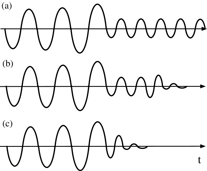
FIG. 19.: Schematic pictures for expected gravitational waveforms during and after the merger for (a) the neutron star formation case; (b) the black hole formation case in which the compactness of the neutron stars before the merger is not very large and the formation timescale is fairly long; (c) the black hole formation case in which the compactness of the neutron stars before the merger is large enough that the formation timescale is short.