Magnetohydrodynamics of Neutrino-cooled Accretion Tori around a Rotating Black Hole in General Relativity

Abstract

We present our first numerical results of axisymmetric magnetohydrodynamic simulations for neutrino-cooled accretion tori around rotating black holes in general relativity. We consider tori of mass $\sim 0.1$–0.4$M_{\odot}$ around a black hole of mass $M=4M_{\odot}$ and spin $a=0$–$0.9M$; such systems are candidates for the central engines of gamma-ray bursts (GRBs) formed after the collapse of massive rotating stellar cores and the merger of a black hole and a neutron star. In this paper, we consider the short-term evolution of a torus for a duration of $\approx 60$ ms, focusing on short-hard GRBs. Simulations were performed with a plausible microphysical equation of state that takes into account neutronization, the nuclear statistical equilibrium of a gas of free nucleons and $\alpha$-particles, black body radiation, and a relativistic Fermi gas (neutrinos, electrons, and positrons). Neutrino-emission processes, such as $e^{\pm}$ capture onto free nucleons, $e^{\pm}$ pair annihilation, plasmon decay, and nucleon-nucleon bremsstrahlung are taken into account as cooling processes. Magnetic braking and the magnetorotational instability in the accretion tori play a role in angular momentum redistribution, which causes turbulent motion, resultant shock heating, and mass accretion onto the black hole. The mass accretion rate is found to be $\dot{M}_{*}\sim 1$–$10M_{\odot}$/s, and the shock heating increases the temperature to $\sim 10^{11}$ K. This results in a maximum neutrino emission rate of $L_{\nu}=$ several $\times 10^{53}$ ergs/s and a conversion efficiency $L_{\nu}/\dot{M}_{*}c^{2}$ on the order of a few percent for tori with mass $M_{\rm t}\approx 0.1$–0.4$M_{\odot}$ and for moderately high black hole spins. These results are similar to previous results in which the phenomenological $\alpha$-viscosity prescription with the $\alpha$-parameter of $\alpha_{v}=0.01$–0.1 is used. It is also found that the neutrino luminosity can be enhanced by the black hole spin, in particular for large spins, i.e., $a\mathrel{\raise 1.29167pt\hbox{$>$}\mkern-14.0mu\lower 2.58334pt\hbox{$\sim$}}0.75M$; if the accretion flow is optically thin with respect to neutrinos, the conversion efficiency may be $\mathrel{\raise 1.29167pt\hbox{$>$}\mkern-14.0mu\lower 2.58334pt\hbox{$\sim$}}10\%$ for $a\mathrel{\raise 1.29167pt\hbox{$>$}\mkern-14.0mu\lower 2.58334pt\hbox{$\sim$}}0.9M$. Angular momentum transport, and the resulting shock heating caused by magnetic stress induce time-varying neutrino luminosity, which is a favorable property for explaining the variability of the luminosity curve of GRBs.

1 Introduction

There is growing evidence that gamma-ray bursts (GRBs) occur at cosmological distances. Assuming the isotropic emission of gamma-rays, the estimated absolute luminosity of many events is $\mathrel{\raise 1.29167pt\hbox{$>$}\mkern-14.0mu\lower 2.58334pt\hbox{$\sim$}}10^{51}$ ergs/s.[1] If the effect of anisotropy, such as the collimation of emission, is taken into account, the luminosity is estimated to be $\sim 10^{50}$ ergs/s. Furthermore, the duration of the emission is very short, $\sim 0.01$–1000 s, indicating that the source is composed of a compact object of stellar-mass size.[1] Thus, the high luminosity can be explained by considering the conversion of energy from gravitational energy to thermal energy during accretion processes onto the compact object. Because a rotating black hole is the most efficient generator, it is now widely believed that the central engines of GRBs are composed of stellar-mass rotating black holes and massive, compact, and hot accretion disks (or tori).

Over the past decade, many groups have studied the properties of dense, hot accretion disks (or tori) around a black hole [e.g., Refs. GRB1,GRB2,GRB3,KM,GRB3.5,GRB4,SRJ,LRP]. An often employed method of study is to derive a stationary solution of accretion flow around a black hole, taking into account the detailed microphysics, but neglecting the effects of the thickness of the disks. [2, 3, 4, 5, 6, 7] Such studies have clarified qualitative and semi-quantitative features of the accretion disks, which are found to be dense, hot, and geometrically thick with maximum density $\sim 10^{12}~{}{\rm g/cm^{3}}$, maximum temperature $\sim 10^{11}$ K, and geometrical thickness $\sim 100$ km for a black hole of mass $\sim 3$–10$M_{\odot}$. Because of the high density and the high temperature, neutrino emission plays a crucial role in the dissipation of thermal energy in such accretion flows, resulting in a high neutrino luminosity of $\mathrel{\raise 1.29167pt\hbox{$>$}\mkern-14.0mu\lower 2.58334pt\hbox{$\sim$}}10^{53}$ erg/s. One important property of this dense, hot accretion flow is that the density is so high that a large fraction of the neutrinos may be trapped by the flow and fail to escape before being swallowed by the black hole; i.e., the accretion flow is neutrino-dominated accretion flow (NDAF). [2, 3, 4]

Although the stationary solutions reveal qualitative properties, these studies are not suitable for understanding the time variability of accretion flows. In the last three years, numerical simulations of viscous and neutrino-cooled accretion tori have also been carried out with detailed microphysics by two groups. [8, 9] Setiawan, Ruffert, and Janka have performed three-dimensional (3D) pseudo-Newtonian simulations with a tabulated equation of state (EOS) derived by Lattimer and Swesty [10] and with a neutrino cooling employing a leakage scheme. As a transport mechanism of angular momentum in the flow, they incorporated a phenomenological viscosity using the so-called $\alpha$-prescription. [11] A general relativistic gravitational field is mimicked using a pseudo-Newtonian potential. They find that the efficiency of the conversion to neutrinos (defined by the ratio of the neutrino luminosity to the rest-mass-energy accretion rate) reaches typically to a few percent with maximum value of $\sim 10\%$. Lee, Ramirez-Ruiz, and Page performed simulations similar to that of Setiawan et al., but with the assumption of axial symmetry, with slightly simplified microphysics, and for a longer time scale of $\approx 0.5$ s. They reported results similar to those of Setiawan et al.

These simulations have provided a variety of nonstationary properties which cannot be found from the study of stationary accretion disks. They have found that the mass accretion rate and neutrino luminosity exhibit a mild time variability. Lee et al. found that the neutrino luminosity decreases on a time scale of 10–1000 ms, depending on the viscous parameter. They also reported that the inhomogeneity of the lepton number induces turbulent motion through a convective instability. These properties can be found only by numerical simulation. This implies that numerical simulation is a better approach for the study of GRB accretion flows.

Despite their success, there are still many issues that have not yet been clarified by simulations. First, the simulations carried out to this time take into account general relativistic effects very crudely, using a pseudo-potential prescription. Although this method may partly capture the nature of general relativistic gravity around black holes, there is no guarantee that this potential can provide quantitatively accurate values concerning properties of black holes. Moreover, special relativistic effects are not incorporated in this method. The speed of matter around black holes is often a significantly large fraction of the speed of light, reaching a high Lorentz factor of $\sim 10$, and hence it is reasonable to expect that the matter motion in the vicinity of a black hole cannot be followed accurately with the pseudo-potential approach. Second, they add a so-called $\alpha$-viscosity in their equations of motion to take into account effects of angular momentum transport and resultant viscous heating. In the $\alpha$-viscosity prescription, one has to a priori determine a value for the $\alpha$-parameter (which is hereafter denoted by $\alpha_{v}$). This parameter essentially fixes the mass accretion rate, the viscous heating rate, and the resulting neutrino luminosity. This implies that one never find these important quantities correctly, due to the unknown value of the $\alpha$-parameter. Most people in the astrophysics currently believe that the magnitude of the viscosity in accretion flows is effectively determined by the turbulent motion of fluid induced by magnetic stress. If this is indeed the case, it implies that the actual effective viscosity varies in time. To capture the nature of a realistic accretion flow, a magnetohydrodynamics (MHD) simulation is needed, instead of adding an $\alpha$-viscosity.

With the motivation described above, we have performed a general relativistic magnetohydrodynamics (GRMHD) simulation using a code recently developed [12], which has already been applied to study the evolution of magnetized differentially rotating neutron stars [13, 14] and magnetized stellar core collapse.[15] In the present work, this code is used for a fixed black hole geometry but with detailed microphysics; a realistic EOS and neutrino cooling. The assumption of the fixed geometry is valid because we consider systems for which the mass of the torus is much smaller than the mass of the black hole. In such systems, the self-gravity of the torus does not play an important role. In the present context, magnetic stress naturally induces time-varying angular momentum transport and shock heating. The rest-mass accretion rate and shock heating rate are computed in a first-principles manner. Furthermore, general relativistic effects are taken into account in a strict manner. Thus, it is possible to clarify the dependence of the neutrino luminosity in the GRB accretion torus on the spin parameter of black holes for the first time in dynamical simulations. In addition, we show that the magnetic effects induce a large time variability of the mass accretion rate and neutrino luminosity, which is not found in simulations employing the $\alpha$-viscosity.

This paper is organized as follows. In §2, we describe the basic equations, EOS, and neutrino processes that we take into account. In §3, the initial conditions and set-up for the simulation are described. In §4, numerical results are presented, focusing particularly on accretion rates of the rest-mass, energy, and angular momentum onto the black hole horizon and on the neutrino luminosity. Varying the masses of the torus and the black hole spin systematically, we clarify the dependence of the accretion rates and neutrino luminosity on these parameters. Section 5 is devoted to a summary and discussion. Throughout this paper, we adopt the geometrical units in which $G=c=1$ where $G$ and $c$ are the gravitational constant and the speed of light. $k$ and $\mathrel{\raise 3.01385pt\hbox{--}\mkern-14.0mu\hbox{$~{}h$}}$ are the Boltzmann and Planck constants. Latin and Greek indices denote spatial components and spacetime components, respectively. $\eta_{\mu\nu}$ and $\delta_{ij}(=\delta^{ij})$ are the flat spacetime metric (in the cylindrical coordinates) and the Kronecker delta, respectively.

2 Procedures for the numerical simulation

We numerically solved GRMHD equations in the fixed geometry of a rotating black hole, assuming that the ideal MHD relation holds; the conductivity is assumed to be infinite. The basic equations and numerical methods are the same as those used in our first paper,[12] except for the EOS and microphysics that we employ. In this section, after we concisely review our basic equations for GRMHD, a detailed description of the EOS and microphysics is given.

2.1 Definition of variables

The fundamental fluid variables are $\rho$, the rest-mass density, $\varepsilon$, the specific internal energy, $P$, the pressure, and $u^{\mu}$, the four velocity. For convenience, we also define the weighted rest-mass density $\rho_{*}$, three-vector $v^{i}$, specific enthalpy $h$, and a Lorentz factor $w$ as

$$\rho_{*}\equiv\rho u^{t}\sqrt{-g/\eta},$$ (1)

$$v^{i}\equiv{dx^{i}\over dt}={u^{i}\over u^{t}},$$ (2)

$$h\equiv 1+\varepsilon+{P\over\rho},$$ (3)

$$w\equiv\alpha u^{t},$$ (4)

where $g$ is the determinant of the spacetime metric $g_{\mu\nu}$, $\eta$ is the determinant of $\eta_{\mu\nu}$, and $\alpha$ is the lapse function equal to $(-g^{tt})^{-1/2}$ (see §2.2).

In addition, we need to define the electron fraction $Y_{e}$ and the temperature $T$ because these are used as arguments for tabulated EOSs (see §2.4 for details). Here, $Y_{e}$ is defined by

$$Y_{e}\equiv{m_{u}n_{e}\over\rho},$$ (5)

where $n_{e}$ is the number density of electrons ($n_{-}$) minus that of positrons ($n_{+}$), and $m_{u}$ is the atomic mass unit.

The only fundamental variable in the ideal MHD is $b^{\mu}$, a four-vector of magnetic field, that is perpendicular to $u^{\mu}$, i.e., $b^{\mu}u_{\mu}=0$. $b^{\mu}$ is regarded as the magnetic field observed in a frame comoving with the fluid. In the ideal MHD, the electric field $E^{\mu}$ in the comoving frame is zero and thus, the electric current $j^{\mu}$ is not necessary to determine the evolution of the field variables. Using $b_{\mu}$, the electromagnetic tensor $F^{\mu\nu}$ is defined by [21]

$$F^{\mu\nu}=\epsilon^{\mu\nu\alpha\beta}u_{\alpha}b_{\beta},$$ (6)

where $\epsilon_{\mu\nu\alpha\beta}$ is the Levi-Civita tensor.

From $b^{\mu}$, we define the three-magnetic field as

$${\cal{B}}^{i}\equiv\alpha\sqrt{\hat{\gamma}}(u^{t}b^{i}-b^{t}u^{i}),$$ (7)

where $\hat{\gamma}=\gamma/\eta$ and $\gamma$ is the determinant of the three-metric $\gamma_{ij}$. ${\cal{B}}^{i}$ is regarded as the magnetic field observed in an inertial frame. We note that ${\cal{B}}^{t}=0$, ${\cal{B}}_{i}=\gamma_{ij}{\cal{B}}^{j}$, and

$$b^{t}={{\cal{B}}^{\mu}u_{\mu}\over\sqrt{-g/\eta}}~{}~{}{\rm and}~{}~{}b_{i}={1\over w\sqrt{\hat{\gamma}}}\Big{(}{\cal{B}}_{i}+{\cal{B}}^{j}u_{j}u_{i}\Big{)}.$$ (8)

Using the hydrodynamic and electromagnetic variables, the energy-momentum tensor is written as

$$T_{\mu\nu}=(\rho h+b^{2})u_{\mu}u_{\nu}+\Big{(}P+{1\over 2}b^{2}\Big{)}g_{\mu\nu}-b_{\mu}b_{\nu},$$ (9)

where

$$b^{2}=b_{\mu}b^{\mu}={{\cal{B}}^{2}+({\cal{B}}^{i}u_{i})^{2}\over w^{2}(-g/\eta)}.$$ (10)

Then, the projection of the energy-momentum tensor is defined by

$$\rho_{\rm H}\equiv T_{\mu\nu}n^{\mu}n^{\nu}=(\rho h+b^{2})w^{2}-P_{\rm tot}-(\alpha b^{t})^{2},$$ (11)

$$J_{i}\equiv-T_{\mu\nu}n^{\mu}\gamma^{\nu}_{~{}i}=(\rho h+b^{2})wu_{i}-\alpha b^{t}b_{i},$$ (12)

$$S_{ij}\equiv T_{\mu\nu}\gamma^{\mu}_{~{}i}\gamma^{\nu}_{~{}j}=(\rho h+b^{2})u_{i}u_{j}+P_{\rm tot}\gamma_{ij}-b_{i}b_{j},$$ (13)

where $n^{\mu}$ is the unit timelike vector normal to a spatial hypersurface, i.e., $\gamma_{\mu\nu}n^{\nu}=0$. Also we define the total pressure $P_{\rm tot}\equiv P+P_{\rm mag}$, where $P_{\rm mag}=b^{2}/2$ is the magnetic pressure.

Using $\rho_{\rm H}$, $J_{i}$, and $S_{ij}$, the energy-momentum tensor is rewritten in the form

$$T_{\mu\nu}=\rho_{\rm H}n_{\mu}n_{\nu}+J_{i}\gamma^{i}_{~{}\mu}n_{\nu}+J_{i}\gamma^{i}_{~{}\nu}n_{\mu}+S_{ij}\gamma^{i}_{~{}\mu}\gamma^{j}_{~{}\nu}.$$ (14)

This form of the energy-momentum tensor is useful for deriving the basic equations for GRMHD presented in §2.3. For the following treatment, we define

$$S_{0}\equiv\sqrt{\hat{\gamma}}\rho_{\rm H}~{}~{}{\rm and}~{}~{}S_{i}\equiv\sqrt{\hat{\gamma}}J_{i}.$$ (15)

We determined the evolution of these variables together with $\rho_{*}$, $Y_{e}$, and ${\cal{B}}^{i}$ in the numerical simulation (see §2.3).

2.2 Gravitational field

The GRMHD equations are solved in a fixed stationary gravitational field of a Kerr black hole. Following Refs. GMT and MG, we choose the Kerr-Schild coordinates of the Kerr black hole, because they have no coordinate singularity on the event horizon, and hence, regular solutions can be obtained even on the event horizon and slightly inside it.

In cylindrical coordinates $(\varpi,z,\varphi)$, the line element of the Kerr-Schild solution is [22]

$$ds^{2}=-dt^{2}+d\varpi^{2}+\varpi^{2}d\varphi^{2}+dz^{2}$$

$$~{}~{}~{}~{}~{}~{}+{2Mr^{3}\over r^{4}+a^{2}z^{2}}\Biggl{(}{r\varpi d\varpi-a\varpi^{2}d\varphi\over r^{2}+a^{2}}+{zdz\over r}+dt\Biggr{)}^{2},$$ (16)

where $r$ is the radial coordinate in the Boyer-Lindquist coordinates, which is the positive solution of the equation

$$r^{4}-(\varpi^{2}+z^{2}-a^{2})r^{2}-a^{2}z^{2}=0.$$ (17)

Here, $M$ and $a$ are the mass and the spin parameter of the Kerr black hole. A physical singularity of ring shape is located at $\varpi=a$ and $z=0$, and the event horizon is at $r=M+\sqrt{M^{2}-a^{2}}\equiv r_{\rm H}$. We note that the determinant of the spacetime metric $g_{\mu\nu}$ has the simple form

$$g=-\varpi^{2}.$$ (18)

For the Kerr-Schild solution, the lapse function $\alpha$, the shift vector $\beta^{i}$, and the three-metric $\gamma_{ij}$ are

$$\alpha=\sqrt{{f\over f+2Mr^{3}}},$$ (19)

$$\beta^{\varpi}={2Mr^{4}\varpi\over\sigma(f+2Mr^{3})},~{}\beta^{z}={2Mr^{2}z\varpi\over f+2Mr^{3}},~{}\beta^{\varphi}=-{2Mar^{3}\over\sigma(f+2Mr^{3})},$$ (20)

$$\gamma_{\varpi\varpi}=1+{2Mr^{5}\varpi^{2}\over f\sigma^{2}},~{}\gamma_{\varpi\varphi}=-{2Mar^{4}\varpi^{3}\over f\sigma^{2}},~{}\gamma_{\varpi z}={2Mr^{3}\varpi z\over f\sigma},$$

$$\gamma_{\varphi\varphi}=\varpi^{2}\Big{(}1+{2Ma^{2}r^{3}\varpi^{2}\over f\sigma^{2}}\Big{)},~{}\gamma_{\varphi z}=-{2Mar^{2}z\varpi^{2}\over f\sigma},~{}\gamma_{zz}=1+{2Mrz^{2}\over f},$$ (21)

where $f\equiv r^{4}+a^{2}z^{2}$ and $\sigma\equiv r^{2}+a^{2}$. The determinant of $\gamma_{ij}$ is

$$\gamma=-{g\over\alpha^{2}}=\varpi^{2}\Big{(}1+{2Mr^{3}\over f}\Big{)}.$$ (22)

2.3 GRMHD equations

Hydrodynamic equations to be solved are

$$\nabla_{\mu}(\rho u^{\mu})=0,$$ (23)

$$\gamma_{i}^{~{}\nu}\nabla_{\mu}T^{\mu}_{~{}\nu}=-Q_{\mu}\gamma_{i}^{~{}\mu},$$ (24)

$$n^{\nu}\nabla_{\mu}T^{\mu}_{~{}\nu}=-Q_{\mu}n^{\mu}.$$ (25)

The first, second, and third equations are the continuity, Euler, and energy equations, respectively. Here, $Q_{\mu}$ denotes a four-dimensional vector associated with neutrino cooling which is defined below, and $\nabla_{\mu}$ is the covariant derivative with respect to $g_{\mu\nu}$. In the following, the equations are described in the cylindrical coordinates $(\varpi,z,\varphi)$ with the assumption of axial symmetry, and we define $S_{y}\equiv S_{\varphi}/\varpi$, $u_{y}=u_{\varphi}/\varpi$, and ${\cal{B}}^{y}\equiv{\cal{B}}^{\varphi}\varpi$.

With the quantities defined above, Eqs. (23)–(25) are written

$$\partial_{t}\rho_{*}+{1\over\varpi}\partial_{\varpi}(\rho_{*}v^{\varpi}\varpi)+\partial_{z}(\rho_{*}v^{z})=0,$$ (26)

$$\partial_{t}S_{A}+{1\over\varpi}\partial_{\varpi}\Big{[}\varpi\Big{\{}S_{A}v^{\varpi}+P_{\rm tot}\delta_{A}^{~{}\varpi}-{1\over(u^{t})^{2}}{\cal{B}}^{\varpi}\Big{(}{\cal{B}}_{A}+u_{A}{\cal{B}}^{i}u_{i}\Big{)}\Big{\}}\Big{]}$$

$$~{}~{}~{}~{}~{}~{}~{}~{}~{}+\partial_{z}\Big{[}S_{A}v^{z}+P_{\rm tot}\delta_{A}^{~{}z}-{1\over(u^{t})^{2}}{\cal{B}}^{z}({\cal{B}}_{A}+u_{A}{\cal{B}}^{i}u_{i})\Big{]}$$

$$~{}~{}~{}~{}~{}~{}~{}~{}~{}=-S_{0}\partial_{A}\alpha+S_{k}\partial_{A}\beta^{k}-{1\over 2}S_{ik}\partial_{A}\gamma^{ik}+{P_{\rm tot}\over\varpi}\delta_{A}^{~{}\varpi}-Q_{A},$$ (27)

$$\partial_{t}S_{y}+{1\over\varpi^{2}}\partial_{\varpi}\Big{[}\varpi^{2}\Big{\{}S_{y}v^{\varpi}-{1\over(u^{t})^{2}}{\cal{B}}^{\varpi}\Big{(}{\cal{B}}_{y}+u_{y}{\cal{B}}^{i}u_{i}\Big{)}\Big{\}}\Big{]}$$

$$~{}~{}~{}~{}~{}~{}~{}~{}~{}+\partial_{z}\Big{[}S_{y}v^{z}-{1\over(u^{t})^{2}}{\cal{B}}^{z}\Big{(}{\cal{B}}_{y}+u_{y}{\cal{B}}^{i}u_{i}\Big{)}\Big{]}=-Q_{y},$$ (28)

$$\partial_{t}S_{0}+{1\over\varpi}\partial_{\varpi}\Big{[}\varpi\Big{\{}S_{0}v^{\varpi}+\sqrt{\hat{\gamma}}P_{\rm tot}(v^{\varpi}+\beta^{\varpi})-{1\over u^{t}\sqrt{\hat{\gamma}}}{\cal{B}}^{i}u_{i}{\cal{B}}^{\varpi}\Big{\}}\Big{]}$$

$$~{}~{}~{}~{}~{}~{}~{}~{}~{}+\partial_{z}\Big{[}S_{0}v^{z}+\sqrt{\hat{\gamma}}P_{\rm tot}(v^{z}+\beta^{z})-{1\over u^{t}\sqrt{\hat{\gamma}}}{\cal{B}}^{i}u_{i}{\cal{B}}^{z}\Big{]}$$

$$~{}~{}~{}~{}~{}~{}~{}~{}~{}~{}=S_{ij}K^{ij}-S_{k}D^{k}\alpha+Q_{\mu}n^{\mu},$$ (29)

where we use $g=-\varpi^{2}$. The subscript $A$ denotes $\varpi$ or $z$, and $i,j,k,\cdots$ are $\varpi$, $z$ or $\varphi$. Also, $K_{ij}$ is the extrinsic curvature, which is calculated in the stationary space from

$$K_{ij}={1\over 2\alpha}\biggl{(}D_{i}\beta_{j}+D_{j}\beta_{i}\biggr{)},$$ (30)

where $D_{i}$ is the covariant derivative with respect to $\gamma_{ij}$. Equations (26)–(29) are solved in the method described in Ref. SS05; we employ a high-resolution scheme consisting of the central scheme proposed by Kurganov and Tadmor [19] with third-order cell-reconstruction. [20]

In addition to the hydrodynamic equations, we solve the evolution equation for $Y_{e}$,

$${dY_{e}\over dt}=-\gamma_{e},$$ (31)

where $\gamma_{e}$ is the capture rate of the electron whose definition is given in §2.4. Using the continuity equation, Eq. (31) can be rewritten as

$$\nabla_{\mu}(\rho Y_{e}u^{\mu})=-\rho u^{t}\gamma_{e},$$ (32)

or, more explicitly,

$$\partial_{t}(\rho_{*}Y_{e})+{1\over\varpi}\partial_{\varpi}(\rho_{*}Y_{e}v^{\varpi}\varpi)+\partial_{z}(\rho_{*}Y_{e}v^{z})=-\rho_{*}\gamma_{e}.$$ (33)

We numerically solved Eq. (33) in the same manner as Eq. (26).

When the ideal MHD relation holds, the Maxwell equations for the axisymmetric system are

$${1\over\varpi}\partial_{\varpi}(\varpi{\cal{B}}^{\varpi})+\partial_{z}{\cal{B}}^{z}=0,$$ (34)

$$\partial_{t}{\cal{B}}^{\varpi}=-\partial_{z}({\cal{B}}^{\varpi}v^{z}-{\cal{B}}^{z}v^{\varpi}),$$ (35)

$$\partial_{t}{\cal{B}}^{z}={1\over\varpi}\partial_{\varpi}\Big{[}\varpi({\cal{B}}^{\varpi}v^{z}-{\cal{B}}^{z}v^{\varpi})\Big{]},$$ (36)

$$\partial_{t}{\cal{B}}^{y}=\partial_{\varpi}({\cal{B}}^{\varpi}v^{y}-{\cal{B}}^{y}v^{\varpi})+\partial_{z}({\cal{B}}^{z}v^{y}-{\cal{B}}^{y}v^{z}).$$ (37)

Equation (34) is the no-monopoles constraint, and Eqs. (35)–(37) are induction equations, which are solved to obtain the evolution of the magnetic field in the same manner as in Ref. SS05, using the constraint transport scheme [26] with a second-order accurate interpolation.

The validity of the numerical code for the GRMHD equations was verified with several test simulations. The numerical results for standard test problems in relativistic MHD, including special relativistic magnetized shocks, general relativistic magnetized Bondi flow in stationary spacetime, and a long-term evolution for a magnetized disk in full general relativity are presented in Ref. SS05.

After solving for the evolution of $\rho_{*}$, $S_{i}$, $S_{0}$, and $Y_{e}$ together with ${\cal{B}}^{i}$, we have to determine the primitive variables, such as $\rho$, $\varepsilon$, $u_{i}$, and $u^{t}$ (or $w=\alpha u^{t}$). The first step in this procedure is to derive the following equation from the definition of $S_{i}$:

$$s^{2}\equiv\rho_{*}^{-2}\gamma^{ij}S_{i}S_{j}=(B^{2}+hw)^{2}(1-w^{-2})-D^{2}(hw)^{-2}(B^{2}+2hw).$$ (38)

Here, $B^{2}$ and $D^{2}$ are determined from the variables $(\rho_{*},S_{i},{\cal{B}}^{i})$ as

$$B^{2}={{\cal{B}}^{2}\over\rho_{*}\sqrt{\hat{\gamma}}}~{}~{}~{}{\rm and}~{}~{}~{}D^{2}={({\cal{B}}^{i}S_{i})^{2}\over\rho_{*}^{3}\sqrt{\hat{\gamma}}},$$ (39)

and to obtain Eq. (38), we use the relation $S_{i}{\cal{B}}^{i}=\rho_{*}h{\cal{B}}^{i}u_{i}$. Equation (38) is regarded as a function of $hw$ and $w^{-2}$ for given data set of $s^{2}$, $B^{2}$, and $D^{2}$. The definition of $S_{0}$ can also be regarded as a function of $hw$ and $w^{-2}$:

$${S_{0}\over\rho_{*}}=hw-{P\sqrt{\hat{\gamma}}\over\rho_{*}}+B^{2}-{1\over 2}\Big{[}B^{2}w^{-2}+D^{2}(hw)^{-2}\Big{]}.$$ (40)

Thus, Eqs. (38) and (40) constitute simultaneous equations for $hw$ and $w$ for given values of $\rho_{*}$, $S_{i}$, $S_{0}$, ${\cal{B}}^{i}$, and $Y_{e}$ at each grid point.

In our previous works [12, 13, 14, 15] in which the $\Gamma$-law or hybrid EOSs are used, a single algebraic equation for $hw$ can be constituted from Eqs. (38) and (40). Then, a Newton-Raphson-type method can be used to obtain $hw$. In this work, we use tabulated EOSs for obtaining $P$, $\varepsilon$, and $h$ (these are functions of $\rho$, $Y_{e}$, and $T$; see §2.4 for details). In such a case, it is not easy to apply the same method, because of the complexity of the EOS. For this reason, we adopt a different iteration method.

At each time step, $\rho_{*}$ and $Y_{e}$ are determined from their evolution equations. Then, $\rho$ should be computed from $\rho_{*}/(\sqrt{\hat{\gamma}}w)$, but $w$ is the variable determined by solving Eqs. (38) and (40). Thus, we guess a solution for $w$ as a first step and calculate a trial solution for $\rho$. For the trial value of $w$, we chose the value of the previous time step. For the resulting values of $\rho$ with $Y_{e}$, Eq. (40) can be regarded as an algebraic equation for $T$, regarding $h$ and $P$ as functions of $T$. Then, searching for the solution from the table, we determine the value of $T$ and, subsequently, $P$, $\varepsilon$, and $h$.

In the iteration, we have to determine a new trial value of $w$. For this purpose, we derive an algebraic equation for $w^{-2}$ from Eqs. (38) and (40):

$$s^{2}=\Big{(}1-{1\over w^{2}}\Big{)}\Big{(}{S_{0}\over\rho_{*}}+{P\sqrt{\hat{\gamma}}\over\rho_{*}}+{B^{2}+D^{2}h^{-2}\over w^{2}}\Big{)}^{2}$$

$$~{}~{}~{}~{}~{}~{}-{D^{2}\over h^{2}w^{2}}\Big{(}-B^{2}+{S_{0}\over\rho_{*}}+{P\sqrt{\hat{\gamma}}\over\rho_{*}}+{B^{2}+D^{2}h^{-2}\over w^{2}}\Big{)}.$$ (41)

If $P$ and $h$ are regarded as given values, this equation is a 3rd-order algebraic equation for $w^{-2}$. Thus, to obtain new trial value of $w$, we solve this equation using the Cardano formula.

We repeat these two procedures until a convergent solution is obtained. In most cases, the solution is obtained within $\sim 10$ iterations. However, in some cases, the solution is not obtained. The problem that often arises is that the solution for $T$ is not found in the EOS table. This happens when $\varepsilon$ accidentally decreases to a small value for which the corresponding value of $T$ is absent in the EOS table. In such a case, we set $T$ to a minimum value that we choose arbitrarily. In the present work, we choose the minimum value to be $10^{9+2/3}$ K (see §2.4).

2.4 Equation of state

Dense, hot accretion tori of mass $\sim 0.1$–1$M_{\odot}$ around a black hole of mass 3–4$M_{\odot}$ are likely outcomes formed after the gravitational collapse of a massive stellar core [28, 29, 30] and after the merger of a low-mass black hole and neutron star, [31, 32, 33] as indicated by numerical simulations. According to the numerical results, the maximum density and temperature of the tori are likely to be $\sim 10^{12}~{}{\rm g/cm^{3}}$ and $T\sim 10^{11}$ K. This temperature is high enough to photo-dissociate heavy nuclei, and hence, the main components of the baryon should be free protons, free neutrons, and $\alpha$-particles. Because of this high temperature, electrons are relativistic and electron-positron pair production is possible in a low-density region. Furthermore, the degeneracy of electrons is high, due to the high density; the chemical potential of the electrons $\mu_{e}$ is comparable to or larger than $kT$. Photons are strongly coupled to the charged particles, and hence, are trapped and advect with the matter flow. Neutrinos are also trapped in the high-density region with $\rho\mathrel{\raise 1.29167pt\hbox{$>$}\mkern-14.0mu\lower 2.58334pt\hbox{$\sim$}}10^{11}~{}{\rm g/cm^{3}}$, whereas, for the low-density region, they escape freely from the tori and this contributes to the cooling process.

We determine the EOS, considering the physical conditions mentioned above. Our approach is similar to that of Ref. LRP. We assume that the torus is composed of free protons, free neutrons, $\alpha$-particles, electrons, positrons, neutrinos, and radiation. Then, the pressure is written

$$P=P_{e}+P_{g}+P_{r}+P_{\nu},$$ (42)

where $P_{e}$, $P_{g}$, $P_{r}$, and $P_{\nu}$ are the pressures of electrons and positrons, of baryons, of the radiation, and of neutrinos.

In the following, we assume that the temperature is high enough ($T\mathrel{\raise 1.29167pt\hbox{$>$}\mkern-14.0mu\lower 2.58334pt\hbox{$\sim$}}10^{10}$ K) that the electrons and positrons are relativistic (i.e., $kT\gg m_{e}c^{2}$, where $m_{e}$ is the electron mass). Then, the total pressure of the electrons and positrons can be determined analytically: [34]

$$P_{e}={(kT)^{4}\over 12\pi^{2}(\mathrel{\raise 3.01385pt\hbox{--}\mkern-14.0mu\hbox{$~{}h$}}c)^{3}}\biggl{[}\eta_{e}^{4}+2\pi^{2}\eta_{e}^{2}+{7\pi^{4}\over 15}\biggr{]},$$ (43)

where $\eta_{e}\equiv\mu_{e}/kT$. The number densities of electrons and positrons, $n_{-}$ and $n_{+}$, are related so as to give an electron fraction $Y_{e}$ of

$${\rho Y_{e}\over m_{u}}=n_{-}-n_{+}={(kT)^{3}\over 3\pi^{2}(\mathrel{\raise 3.01385pt\hbox{--}\mkern-14.0mu\hbox{$~{}h$}}c)^{3}}\Big{[}\eta_{e}^{3}+\eta_{e}\pi^{2}\Big{]}.$$ (44)

We note that the assumption $kT\gg m_{e}c^{2}$ is not always valid, but for the dense region of the torus in which we are interested, it holds approximately.[9] Equations (43) and (44) hold for arbitrary degeneracy as long as the temperature is high enough.

The gas and radiation pressure are written

$$P_{g}={\rho kT\over m_{u}}{1+3X_{\rm nuc}\over 4},$$ (45)

$$P_{r}={a_{r}T^{4}\over 3},$$ (46)

where $X_{\rm nuc}$ is the mass fraction of free nucleons and $a_{r}$ the radiation density constant ($\pi^{2}k^{4}/15(\mathrel{\raise 3.01385pt\hbox{--}\mkern-14.0mu\hbox{$~{}h$}}c)^{3}$). If the neutrinos of all species are in thermal equilibrium with the matter, the neutrino pressure is given by

$$P_{\nu}={7\over 8}a_{r}T^{4},$$ (47)

whereas the pressure is negligible if they are transparent. In this paper, we follow the treatment of Ref. LRP and set

$$P_{\nu}={7\over 8}a_{r}T^{4}(1-e^{-\tau_{\nu}}),$$ (48)

where $\tau_{\nu}$ is the averaged optical depth of the neutrinos.

In the present context, the ratio of the radiation pressure to the gas pressure is

$${P_{r}\over P_{g}}=3.0\times 10^{-2}T_{11}^{3}\rho_{12}^{-1},$$ (49)

where $T_{11}=T/10^{11}$ K, $\rho_{12}=\rho/10^{12}~{}{\rm g/cm^{3}}$, and we assume that $X_{\rm nuc}=1$. For the case that the electron is degenerate with $\eta_{e}\sim 10$, the ratio of the electron pressure to the gas pressure is

$${P_{e}\over P_{g}}\approx 1.2\times 10^{1}T_{11}^{3}\rho_{12}^{-1}\Big{(}{\eta_{e}\over 10}\Big{)}^{4}.$$ (50)

Thus, in the main body of the torus with $T_{11}=O(1)$ and $\rho_{12}=O(1)$, the gas pressure is the dominant pressure source if the electrons are mildly degenerate with $\eta_{e}\mathrel{\raise 1.29167pt\hbox{$<$}\mkern-14.0mu\lower 2.58334pt\hbox{$\sim$}}5$, whereas for the case that the electrons are strongly degenerate, the degenerate pressure is dominant.

The specific internal energy is written

$$\varepsilon=\varepsilon_{e}+\varepsilon_{g}+\varepsilon_{r}+\varepsilon_{\nu},$$ (51)

where each term is related to the pressure by

$$\varepsilon_{e}={3P_{e}\over\rho},~{}~{}\varepsilon_{g}={3P_{g}\over 2\rho},~{}~{}\varepsilon_{r}={3P_{r}\over\rho},~{}~{}\varepsilon_{\nu}={3P_{\nu}\over\rho}.$$ (52)

The pressure and specific internal energy should be provided for given values of $\rho$, $T$, and $Y_{e}$. For this purpose, the chemical potential of electrons, $\mu_{e}$, and the free nucleon fraction, $X_{\rm nuc}$, have to be written as functions of $(\rho,T,Y_{e})$. Equation (44) is used to obtain the functional form of the chemical potential. Then, for simplicity, we use a fitting formula [35] for the mass fraction of the free nucleon,

$$X_{\rm nuc}={\rm Min}\Big{(}22.4T_{10}^{9/8}\rho_{10}^{-3/4}\exp(-8.2/T_{10}),1\Big{)},$$ (53)

where $T_{10}=T/10^{10}$ K and $\rho_{10}=\rho/10^{10}~{}{\rm g/cm^{3}}$.

We tabulated an EOS table for the ranges $\rho_{\rm min}\leq\rho\leq 10^{13}~{}{\rm g/cm^{3}}$ and $T_{\rm min}\leq T\leq 5\times 10^{11}~{}{\rm K}$. The values $\rho_{\rm min}$ and $T_{\rm min}$ are the minimum values that we arbitrarily chose to maintain the stability of the numerical computation. Because the temperature should not be much smaller than $m_{e}c^{2}/k$, because of our assumption that the electrons are relativistic, we set the value of $T_{\rm min}$ to $10^{9+2/3}$ K. The value of $\rho_{\rm min}$ is specified in §3.4.

2.5 Neutrino emission

Several processes contribute to the emission of neutrinos. The most important ones in the present context are the electron and positron captures onto free nucleons:

$$p+e^{-}\rightarrow n+\nu_{e},$$ (54)

$$n+e^{+}\rightarrow p+\bar{\nu}_{e}.$$ (55)

These processes change the electron fraction. Assuming that the electrons and positrons are relativistic, the electron capture rate in the optically thin region for neutrinos is approximately given by (see Appendix B)

$$\gamma_{e0}=K_{c}\biggl{(}{kT\over m_{e}c^{2}}\biggr{)}^{5}[F_{4-}(\eta_{e})X_{p}-F_{4+}(\eta_{e})X_{n}],$$ (56)

where $X_{p}$ and $X_{n}$ are the mass fractions of free protons and free neutrons, $K_{c}=\ln 2/10^{3.035}~{}{\rm s}^{-1}$, and

$$F_{4-}(x)=45.59x+{2\pi^{2}\over 3}x^{3}+{1\over 5}x^{5}+24\biggl{(}e^{-x}-{1\over 32}e^{-2x}+{1\over 243}e^{-3x}\biggr{)},$$ (57)

$$F_{4+}(x)=24\biggl{(}e^{-x}-{1\over 32}e^{-2x}+{1\over 243}e^{-3x}\biggr{)}.$$ (58)

In the optically thick region for neutrinos, $\beta$-equilibrium is assumed to be satisfied and the electron fraction does not change. In this paper, we simply multiply by $e^{-\tau_{\nu}}$ in order to take into account the opacity effect (diffusion effect) and define the electron capture rate by

$$\gamma_{e}=\gamma_{e0}e^{-\tau_{\nu}}.$$ (59)

We note that the actual optical depth depends on the neutrino species and neutrino energy. In this paper, we ignore such a dependence.

As a result of the electron and positron captures, neutrinos are emitted and they carry away thermal energy of the rate

$$\dot{Q}_{\rm cap}=K_{c}{m_{e}\over m_{u}}\rho c^{2}\biggl{(}{kT\over m_{e}c^{2}}\biggr{)}^{6}[F_{5-}(\eta_{e})X_{p}+F_{5+}(\eta_{e})X_{n}],$$ (60)

where

$$F_{5-}(x)=236.65+{7\pi\over 6}x^{2}+{5\pi^{2}\over 6}x^{4}+{1\over 6}x^{6}$$

$$~{}~{}~{}~{}-120\biggl{(}e^{-x}-{1\over 64}e^{-2x}+{1\over 729}e^{-3x}\biggr{)},$$ (61)

$$F_{5+}(x)=120\biggl{(}e^{-x}-{1\over 64}e^{-2x}+{1\over 729}e^{-3x}\biggr{)}.$$ (62)

In addition to electron and positron captures, we consider the annihilation of electron-positron pairs into thermal neutrinos, nucleon-nucleon bremsstrahlung, and plasmon decay. For the neutrino emissivity due to electron-positron pair annihilation, we use the fitting formula derived by Itoh et al. [36] For the other two, we write the emissivity as [e.g., Refs. KM,Itoh, and RJ]

$$\dot{Q}_{\rm ff}=1.5\times 10^{31}T_{11}^{5.5}\rho_{12}^{2}~{}~{}{\rm ergs/cm^{3}/s},$$ (63)

$$\dot{Q}_{\rm pla}=1.5\times 10^{32}T_{11}^{9}\gamma_{p}e^{-\gamma_{p}}(2+2\gamma_{p}+\gamma_{p}^{2})~{}~{}{\rm ergs/cm^{3}/s},$$ (64)

where $\gamma_{p}=5.565\times 10^{-2}\sqrt{(\pi^{2}+3\eta_{e}^{2})/3}$.[37] Then, we define the total emissivity as

$$\dot{Q}=(\dot{Q}_{\rm cap}+\dot{Q}_{\rm pair}+\dot{Q}_{\rm ff}+\dot{Q}_{\rm pla})e^{-\tau_{\nu}}.$$ (65)

Because $\dot{Q}$ is the emissivity (cooling rate) measured in the fluid rest-frame, we define $Q_{\mu}$ as [38, 39]

$$Q_{\mu}=\dot{Q}u_{\mu}.$$ (66)

With this treatment, the effect of anisotropic emission associated with the matter motion is taken into account. On the other hand, the effects of radiation transfer and the heating due to the emitted neutrinos are ignored.

The main source of opacity for neutrinos is scattering by free nucleons and $\alpha$-particles. For these processes, the order of the cross section is $\sim 10^{-42}T_{11}^{2}~{}{\rm cm^{2}}$. [27] Because the number density of free nucleons is $\sim 10^{35}\rho_{11}~{}{\rm cm^{-3}}$, the mean free path of the neutrinos is roughly

$$\sim 10^{7}~{}T_{11}^{-2}\rho_{11}^{-1}~{}{\rm cm},$$ (67)

which is $\sim 20GM/c^{2}$ for black holes of mass $4M_{\odot}$. In this work, we consider accretion tori of width and thickness $\sim 20$–$30GM/c^{2}$ and maximum temperature $\sim 10^{11}$ K. Hence, we simply set the optical depth to

$$\tau_{\nu}=\zeta\rho_{11},$$ (68)

where $\zeta$ is a constant that we set to 1 or 1/3 [i.e., $\tau_{\nu}=\rho/(10^{11}~{}{\rm g/cm^{3}})$ or $\rho/(3\times 10^{11}~{}{\rm g/cm^{3}})$]. Previous works investigating dense accretion tori (e.g., Ref. LRP) shows that the neutrinos are optically thick when the density satisfies the condition $\rho_{11}\mathrel{\raise 1.29167pt\hbox{$>$}\mkern-14.0mu\lower 2.58334pt\hbox{$\sim$}}1$. Thus, the present treatment can capture the neutrino-trapping effect, at least qualitatively.

2.6 Diagnostics

We monitor the total baryon rest-mass $M_{*}$, angular momentum $J$, internal energy $E_{\rm int}$, rotational kinetic energy $T_{\rm rot}$, and electromagnetic energy $E_{\rm EM}$, which are defined by

$$M_{*}=\int\rho_{*}\sqrt{\eta}d^{3}x,$$ (69)

$$J=\int\rho_{*}hu_{\varphi}\sqrt{\eta}d^{3}x,$$ (70)

$$E_{\rm int}=\int\rho_{*}\epsilon\sqrt{\eta}d^{3}x,$$ (71)

$$T_{\rm rot}=\int{1\over 2}\rho_{*}h\Omega u^{t}u_{\varphi}\sqrt{\eta}d^{3}x,$$ (72)

$$E_{\rm EM}=\int T_{\rm EM}^{tt}\alpha\sqrt{\eta}d^{3}x,$$ (73)

where $T_{\rm EM}^{\mu\nu}$ is the electromagnetic part of the energy-momentum tensor, $\Omega$ is the angular velocity defined by $u^{\varphi}/u^{t}$, and all the integrations are performed outside the event horizon. For the definitions of $E_{\rm int}$, $T_{\rm rot}$, and $E_{\rm EM}$, we follow Ref. DLSSS2.

In stationary axisymmetric spacetime, the following relations are derived from the conservation law of the energy-momentum tensor in the absence of neutrino cooling:

$$\partial_{\mu}\sqrt{-g}T^{\mu}_{~{}t}=0,$$ (74)

$$\partial_{\mu}\sqrt{-g}T^{\mu}_{~{}\varphi}=0.$$ (75)

From these relations, it is natural to define the energy and angular momentum accretion rates by the surface integral at the event horizon as

$$\dot{E}=\oint_{r=r_{\rm H}}T^{r}_{~{}t}\sqrt{-g}dS,$$ (76)

$$\dot{J}=-\oint_{r=r_{\rm H}}T^{r}_{~{}\varphi}\sqrt{-g}dS,$$ (77)

where $dS=d\theta d\varphi$. From the continuity equation, the rest-mass accretion rate is defined in the same manner as

$$\dot{M}_{*}=-\oint_{r=r_{\rm H}}\rho_{*}v^{r}r_{\rm H}^{2}dS.$$ (78)

Because we adopt cylindrical coordinates in the Kerr-Schild coordinates, grid points are not located at $r=r_{\rm H}$. To obtain the values there, we use linear interpolations for all the necessary quantities.

In the presence of neutrino cooling, Eq. (74) is written

$$\partial_{\mu}\sqrt{-g}T^{\mu}_{~{}t}=-\sqrt{-g}\dot{Q}u_{t}.$$ (79)

Thus, the rate of energy loss by the neutrinos is given by

$$L_{\nu}=-\int_{r>r_{\rm H}}\sqrt{-g}u_{t}\dot{Q}d^{3}x.$$ (80)

We refer to $L_{\nu}$ simply as the neutrino luminosity. Strictly speaking, $L_{\nu}$ is the sum of the energy emission rates of neutrinos toward infinity and toward the black hole horizon. Thus, the luminosity observed at infinity is smaller than this value, because a finite fraction of neutrinos emitted at each radius is always swallowed by the black hole. To roughly infer how much neutrino energy is likely to be swallowed by black holes, we also compute the quantity

$$L_{\nu}(r_{\rm ph})=-\int_{r>r_{\rm ph}}\sqrt{-g}u_{t}\dot{Q}d^{3}x.$$ (81)

where $r_{\rm ph}$ denotes the radius of the limiting circular photon-orbit:[27]

$$r_{\rm ph}=2M\Big{[}1+\cos\Big{\{}{2\over 3}\cos^{-1}(-a/M)\Big{\}}\Big{]}.$$ (82)

This radius is characterized by the fact that 50% of massless particles from a stationary isotropic emitter at $r=r_{\rm ph}$ is captured by the black hole [27]. To compute the luminosity more accurately, it is necessary to multiply by an escape probability that depends on the position and velocity of the emitter. In the present paper, we do not take into account such probability but simply calculate the luminosity using Eq. (80) or (81).

From $\dot{M}_{*}$ and $L_{\nu}$, the total rest-mass swallowed by a black hole and the emitted neutrino energy are defined by

$$\Delta M_{*}(t)=\int_{0}^{t}\dot{M}_{*}dt^{\prime},$$ (83)

$$\Delta E_{\nu}(t)=\int_{0}^{t}L_{\nu}dt^{\prime}.$$ (84)

In the following, we refer to $\Delta E_{\nu}/\Delta M_{*}$ as the average energy conversion efficiency to neutrinos.

3 Initial conditions and setting for computation

3.1 Initial condition for torus

As the initial conditions, we first prepare equilibrium states of a torus rotating around a black hole with no magnetic field and with no neutrino cooling. Such equilibria are determined from the first integral of the Euler equation, which has already been derived for axisymmetric stationary spacetime.[40, 41] We adopt the prescription of Ref. AJS because of its simplicity. In Kerr-Schild coordinates, the derivation of the basic equations is slightly more complicated than in Boyer-Lindquist coordinates. For example, in Boyer-Lindquist coordinates, we have $u_{\varpi}=u_{z}=0$, whereas they are nonzero in Kerr-Schild coordinates. We have to be careful regarding this point in setting the initial conditions. For completeness, here, we describe the basic equations for obtaining equilibria.

First, we assume that the four-velocity has the following components:

$$u^{\mu}=(u^{t},0,0,u^{\varphi}).$$ (85)

Note that this does not imply that $u_{\varpi}$ and $u_{z}$ are zero, because of the presence of nonzero off-diagonal components of $g_{\mu\nu}$. Defining the angular velocity $\Omega\equiv u^{\varphi}/u^{t}$, the Euler equation in the stationary axisymmetric system is written in the well-known form

$${\partial_{k}u^{t}\over u^{t}}-u^{t}u_{\varphi}\partial_{k}\Omega-{\partial_{k}P\over\rho h}=0.$$ (86)

In the method of Ref. AJS, one assumes

$$\ell=-{u_{\varphi}\over u_{t}}={\rm const}.$$ (87)

Then, Eq. (86) can be rewritten as

$$(\partial_{k}u_{t})u^{t}(1-\ell\Omega)-{\partial_{k}P\over\rho h}=0.$$ (88)

Now, $u^{t}u_{t}+u^{\varphi}u_{\varphi}=-1$ gives $u^{t}(1-\ell\Omega)=-1/u_{t}$. Thus, we obtain

$$\partial_{k}\ln(-u_{t})+{\partial_{k}P\over\rho h}=0.$$ (89)

If we assume that the fluid is isentropic, the first law of thermodynamics is used to rewrite the second term as $\partial_{k}\ln(h)$. Thus, we obtain the first integral of the Euler equation in the same form as that in Ref. AJS,

$$hu_{t}=C,$$ (90)

where $C$ is an integration constant. Then, using the relation

$$\Omega=-{g_{tt}\ell+g_{t\varphi}\over g_{t\varphi}\ell+g_{\varphi\varphi}},$$ (91)

we obtain

$$u_{t}=-\biggl{(}{g_{t\varphi}^{2}-g_{tt}g_{\varphi\varphi}\over g_{\varphi\varphi}+2g_{t\varphi}\ell+g_{tt}\ell^{2}}\biggr{)}^{1/2}.$$ (92)

Hence, $h$ at each point is determined from Eq. (90) for given values of $\ell$ and $C$.

Specifically, the configuration of tori is determined by fixing the inner and outer edges on the equatorial plane. We denote the cylindrical coordinate radii of these edges by $\varpi_{1}$ and $\varpi_{2}~{}(>\varpi_{1})$. The condition $h=1$ at $\varpi=\varpi_{1}$ and $\varpi_{2}$ determines the values of $C$ and $\ell$ using Eqs. (90) and (92). Subsequently, the profile for $h$ is determined from Eq. (90).

To derive $\rho$ and $P$ from $h$, the EOS table is used. In doing so, we have to further assume relations among $\rho$, $Y_{e}$, and $T$, because $h$ is a function of these three arguments in the table. In the present paper, we assume that $T=10^{10}$ K uniformly in all regions. Because the tori and its atmosphere formed after stellar core collapse and the merger of compact objects are likely to be moderately hot at their formation, this assumption is reasonable. To determine $Y_{e}$, we use the prescription of Ref. LRP: For optically thick regions, we assume that $\beta$-equilibrium holds, i.e.,

$$p+e^{-}\leftrightarrow n+\nu_{e},$$ (93)

and hence, the ratio of the proton fraction to the neutron fraction is assumed to be

$${X_{p}\over X_{n}}=e^{(Q-\mu_{e})/kT},$$ (94)

where $Q=1.293$ MeV is the difference between the neutron and proton masses. Here, we assume that the chemical potential of neutrinos is zero for simplicity.

For optically thin regions, we assume that the reaction rates of the processes given in Eqs. (54) and (55) are identical and that the number densities of protons and neutrons are unchanged.[42] Under these assumptions, the electron fraction is approximately given by [see Eq. (12) of Ref. LRP]

$$Y_{e}={1-X_{\rm nuc}\over 2}+X_{\rm nuc}\biggl{[}\biggl{(}{1\over 2}+0.487{Q/2-\mu_{e}\over kT}\biggr{)}e^{-\tau_{\nu}}$$

$$~{}~{}~{}~{}~{}~{}~{}~{}~{}~{}~{}~{}~{}~{}~{}~{}~{}~{}~{}~{}~{}~{}~{}~{}~{}~{}~{}~{}~{}+{1\over 1+e^{(\mu_{e}-Q)/kT}}(1-e^{-\tau_{\nu}})\biggr{]},$$ (95)

where for $X_{\rm nuc}$, Eq. (53) is used. In this rule with $T_{10}=1$, $Y_{e}$ is smaller than 0.5 for high-density regions with $\rho\mathrel{\raise 1.29167pt\hbox{$>$}\mkern-14.0mu\lower 2.58334pt\hbox{$\sim$}}10^{11}~{}{\rm g/cm^{3}}$, whereas for low-density regions, it is larger than 0.5.

The initial conditions obtained with the present method are not isentropic although we assume isentropic conditions in deriving Eq. (90). Thus, the torus is not exactly in equilibrium. However, in the test simulations with no magnetic field and no neutrino cooling, we found that the torus approximately remains in the initial state even after the density maximum orbits the black hole for 10 rotational periods. With this test, we confirmed that the initial conditions adopted in this method are approximately in equilibrium.

There are several free parameters for determining the initial conditions: The black hole mass, $M$, the black hole spin, $a$, the mass of the torus, $M_{*}$, and the density profile of the torus. We fix the black hole mass to $4M_{\odot}$. Such a black hole is a plausible outcome, forming soon after the stellar core collapse of massive star and after the merger of black hole-neutron star binaries. Because we do not know a plausible value of the black hole spin, numerical computations were systematically performed for a wide range of $a$. A plausible mass of a torus formed in the vicinity of a black hole is a few tenths of $M_{\odot}$. In the present work, we choose $M_{*}\approx 0.1$–$0.4M_{\odot}$. Because we consider compact tori rotating around a black hole, the inner edge of the torus is chosen to be slightly outside of the radius of the innermost stable circular orbit (ISCO) as $\varpi_{1}=5$–$7M$. Then, for a fixed value of $M_{*}$, the location of the outer edge is automatically determined to be $\approx 30$–40$M$ for an $\ell=$constant angular momentum profile.

In Table I, we list parameter values for selected models adopted in the numerical simulation. For models A–E, the torus mass is approximately given by $M_{*}\approx 0.25M_{\odot}$, whereas the black hole spins are all different. For models F–J, the black hole spin is fixed to $a/M=0.75$, whereas the mass and inner edges of the torus are different. In Table II, we list the parameters for a test particle orbiting a black hole at the ISCO for several values of $a/M$. These are key quantities for determining the neutrino luminosity and the conversion efficiency of the rest-mass energy to neutrinos (see §4 for discussion).

Table 1: Parameter set for the adopted models. The spin parameter of the black hole, the rest-mass of tori, the coordinate radius of the inner and outer edges, $\varpi_{1}$ and $\varpi_{2}$, of tori, the maximum density of tori, $E_{\rm int}/M_{*}$, $T_{\rm rot}/M_{*}$, $J/M_{*}$, and the rotation period at the density maximum, $P_{c}$, of tori. For every model, the black hole mass is fixed to be $M=4M_{\odot}$, and the ratio of the electromagnetic energy to $E_{\rm int}$ is 1/200. $\varpi_{1}$ and $\varpi_{2}$ are given in units of $M$, and $E_{\rm int}$ and $T_{\rm rot}$ are in units of $M_{*}/100$.

Model	$a/M$	$M_{*}~{}(M_{\odot})$	$\varpi_{1},\varpi_{2}$	$\rho_{\rm max}$(g/cm3)	$E_{\rm int}$	$T_{\rm rot}$	$J/M_{*}$	$P_{c}/M$	$\zeta$
A	0	0.244	6.4, 41	$3.5\times 10^{11}$	$0.85$	$3.3$	$4.03$	248	1
A2	0	0.248	6.4, 41	$3.6\times 10^{11}$	$0.85$	$3.3$	$4.03$	248	1/3
B	0.25	0.240	6 , 36	$4.7\times 10^{11}$	$0.94$	$3.7$	$3.82$	219	1
B2	0.25	0.243	6 , 36	$4.7\times 10^{11}$	$0.93$	$3.7$	$3.82$	219	1/3
C	0.5	0.249	6 , 34	$5.4\times 10^{11}$	$0.99$	$3.7$	$3.70$	207	1
C2	0.5	0.253	6 , 34	$5.5\times 10^{11}$	$0.99$	$3.7$	$3.69$	207	1/3
D	0.75	0.247	6 , 32	$6.1\times 10^{11}$	$1.0$	$3.8$	$3.58$	203	1
D2	0.75	0.251	6 , 32	$6.1\times 10^{11}$	$1.0$	$3.8$	$3.58$	203	1/3
E	0.9	0.247	6 , 31	$6.4\times 10^{11}$	$1.1$	$3.8$	$3.51$	197	1
E2	0.9	0.251	6 , 31	$6.5\times 10^{11}$	$1.1$	$3.8$	$3.51$	197	1/3
F	0.75	0.237	4.8 , 24.6	$1.2\times 10^{12}$	$1.3$	$4.9$	$3.27$	146	1
G	0.75	0.132	6.9 , 33	$2.8\times 10^{11}$	$0.82$	$3.5$	$3.74$	241	1
H	0.75	0.146	6.6, 31.8	$3.4\times 10^{11}$	$0.87$	$3.6$	$3.68$	227	1
I	0.75	0.366	5.4, 31.2	$1.0\times 10^{12}$	$1.2$	$4.1$	$3.45$	173	1
J	0.75	0.397	6.0, 36	$7.8\times 10^{12}$	$1.1$	$3.5$	$3.61$	209	1

Table 2: Quantities for a test particle orbiting a black hole at the ISCO for various values of the black hole spin. The value of the $r$ coordinate of the ISCO, $r_{\rm ISCO}$, the specific energy at the ISCO, $E_{\rm ISCO}$, and the specific angular momentum at ISCO, $J_{\rm ISCO}$. The fifth and sixth columns list $r_{\rm H}$ and $r_{\rm ph}$. Note that the $\varpi$ coordinate on the equatorial plane is related to $r$ by $\varpi=\sqrt{r^{2}+a^{2}}$. In this paper, we refer to $1-E_{\rm ISCO}$ as the specific gravitational binding energy at the ISCO.

$a/M$	$r_{\rm ISCO}/M$	$E_{\rm ISCO}$	$J_{\rm ISCO}/M$	$r_{\rm H}/M$	$r_{\rm ph}/M$
0	6.000	0.9428	3.464	2.000	3.000
0.25	5.156	0.9331	3.221	1.968	2.695
0.50	4.233	0.9179	2.917	1.866	2.347
0.75	3.158	0.8882	2.489	1.661	1.916
0.90	2.321	0.8442	2.100	1.436	1.558

An important feature found from Table I is that for (approximately) fixed values of $M$, $M_{*}$, and the radius of the torus, the maximum density is higher for larger values of $a$ (compare models A–E). It is also found that for fixed values of $M$, $M_{*}$, and $a$, the maximum density is higher for smaller values of the rotation radius of the torus. For larger values of $a$, the radius of the ISCO on the equatorial plane is smaller (see Table II), and hence, the torus can be more compact, thereby increasing the maximum density. All these features imply that for larger values of $a$, the density can be higher. Because the optical depth of neutrinos depends strongly on the density for $\rho\mathrel{\raise 1.29167pt\hbox{$>$}\mkern-14.0mu\lower 2.58334pt\hbox{$\sim$}}10^{11}~{}{\rm g/cm^{3}}$, this dependence of the maximum density on the black hole spin plays an important role in determining the neutrino luminosity.

(a)

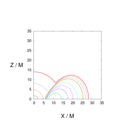
(b)

Figure 1: (a) Density contour curves of initial conditions for model D. The contour curves are drawn for $\rho=10^{12-0.5i}~{}{\rm g/cm^{3}}$ with $i=1$–10. The atmosphere is included in these initial conditions. (b) The same as (a) but for magnetic field lines.

In Fig. 1(a), we plot density contour curves for model D (cf. Table I). It is seen that the torus has a geometrically thick structure in which the width $\varpi_{2}-\varpi_{1}$ is comparable to the maximum thickness, $\sim 30M$. This is a universal property that holds for all the models.

Figure 2 plots the angular velocity $\Omega$ as a function of the cylindrical radius on the equatorial plane. It is found that the torus has a differentially rotating velocity field with the steepness of the differential rotation $|d\ln\Omega/d\ln\varpi|\approx 2$, steeper than the Keplerian law. This is also a feature of the $\ell=$constant velocity profile.

Figure 2: Angular velocity as a function of the cylindrical radius on the equatorial plane for model D.

3.2 Magnetic field

To induce angular momentum transport during the evolution, a weak poloidal magnetic field is initially added to the equilibrium torus. In the present work, the profile of the magnetic field is chosen following Refs. GMT,MG,VH as

$$A_{\varphi}=\Big{\{}\begin{array}[]{ll}A_{0}(\rho-\rho_{0})&{\rm for}~{}\rho\geq\rho_{0},\\ 0&{\rm for}~{}\rho<\rho_{0},\end{array}$$ (98)

where $A_{0}$ is a constant that specifies the magnetic field strength and $\rho_{0}$ is a cut-off density; the magnetic field is initially non-zero only in the region with $\rho>\rho_{0}$. Here, $A_{0}$ is chosen such that the ratio of the magnetic energy to the thermal energy is $1/200$, and $\rho_{0}$ is chosen as $0.2\rho_{\rm max}$, where $\rho_{\rm max}$ is the maximum density of the torus. Because the magnetic field is weak, the equilibrium configuration is not essentially modified by the magnetic force.

In Fig. 1(b), we show the magnetic field lines for model D (cf. Table I). Comparing Fig. 1(a), it is seen that the magnetic field is initially present in a localized region near the density maximum because the density of the torus decreases rapidly in the direction of the surface.

Tori both with the poloidal magnetic field and with differential rotation are subject to winding of the field lines and subsequent magnetic braking [23]. In addition, they are subject to the magnetorotational instability (MRI).[24] Due to the winding of the magnetic field lines, the toroidal magnetic field ${\cal{B}}^{T}$ grows linearly with time in the early phase of the numerical simulation as [e.g., Ref. DLSSS2]

$${\cal{B}}^{T}\approx t{\cal{B}}^{\varpi}{\partial\Omega\over\partial\ln\varpi}\sim-2\Omega t{\cal{B}}^{\varpi}.$$ (99)

This amplification continues until the magnetic energy of the toroidal field becomes a few tenths of the rotational energy (cf. §4.1.1). After the amplification stops, the magnetic braking transports the angular momentum outwards. For the present initial conditions with which $E_{\rm EM}/T_{\rm rot}\sim 0.001$, the field growth saturates when ${\cal{B}}^{T}$ becomes $\sim 30{\cal{B}}^{\varpi}$. This implies that the field growth stops at $t\sim 15\Omega^{-1}\sim 2P_{\rm o}$, where $P_{\rm o}$ denotes the local rotational period. Because the magnetic field is confined near the density maximum, the expected saturation time is $\sim 2$–$3P_{c}$, where $P_{c}$ is the rotation period at the density maximum.

The growth time ($e$-folding time) and wavelength of the fastest-growing mode of the MRI in the Newtonian theory are approximately given by [e.g., Refs. MRI and DLSSS3]

$$t_{\rm MRI}=2\left|{\partial\Omega\over\partial\ln\varpi}\right|^{-1}\ ,$$ (100)

$$\lambda_{\rm max}={2\pi v_{A}^{z}\over\Omega}\biggl{[}1-\biggr{(}{\kappa\over 2\Omega}\biggr{)}^{4}\biggr{]}^{-1/2},$$ (101)

where $\kappa$ is the epicyclic frequency of Newtonian theory,

$$\kappa^{2}\equiv\frac{1}{\varpi^{3}}\frac{\partial(\varpi^{4}\Omega^{2})}{\partial\varpi},$$ (102)

and $v_{A}^{z}\equiv\sqrt{{\cal{B}}^{z}{\cal{B}}_{z}/\rho\hat{\gamma}}$ is the approximate Alfvén velocity of the $z$ component. In general relativity, the growth rate is modified, but it agrees with Eq. (100) within $\sim 30\%$.[25] As in the case of the field winding, the growth time scale of the MRI is of order $P_{c}$. With the present initial conditions, we have $|v_{A}^{z}|\approx 10^{-2}$ and $P_{c}\sim 200M$ at the density maximum (see Table I), resulting in $\lambda_{\rm max}\sim 2M$. Because this is smaller than the width of tori, the MRI should play an important role in transporting the angular momentum and driving the turbulent motion in the accretion torus. We also note that the grid spacing is chosen to be typically $0.15M$, so that the MRI can be resolved in numerical simulations. We note that with the present models as described above, we have $E_{\rm EM}/E_{\rm int}=1/200$. If the magnetic field strength is smaller than its present initial strength by a factor of more than 5–10, then the wavelength $\lambda_{\rm max}$ is too small to be resolved. If the magnetic field strength is chosen to be too large, $\lambda_{\rm max}$ is so large that the MRI does not play an important role. The present choice of the field strength is appropriate for taking into account both the effects of the magnetic braking and the MRI.

It is known that non-magnetized tori with $\ell=$constant is often unstable with respect to the runaway instability (see, e.g., Ref. Font and references cited therein). However, in the present model, the angular momentum of tori is redistributed by the magnetic braking and the MRI on a short time scale of $\sim 2$–$3P_{c}$, and then a quasistationary accretion state, which has a less steep velocity profile, and hence, is stable with respect to the runaway instability, is established. The resulting quasistationary state is expected to depend only weakly on the initial profile of the angular momentum distribution, and thus, the numerical results should not depend strongly on the given velocity profile.

3.3 Preparation of grid and boundary conditions

A numerical simulation is performed in a nested grid zone; we divide the computational domain into three zones and follow each zone with a different grid spacing. The computation in innermost zone is carried out with the finest grid spacing $\Delta$. This zone covers the square domain satisfying $0\leq X\leq 48M$, except for the inner square patch with $0\leq X\leq 0.8r_{\rm H}$, which is excised. Here, $X$ denotes $\varpi$ and $z$. The second and third zones cover $0\leq X\leq 96M$ and $0\leq X\leq 192M$, with the grid spacings $2\Delta$ and $4\Delta$, respectively. At the outer boundaries of the first and second zones, values linear-interpolated from the 1-level larger zone are assigned as the boundary values. Specifically, the interpolation is performed for $\rho_{*}$, $\hat{u}_{i}\equiv hu_{i}$, $T$, $Y_{e}$, and ${\cal{B}}^{i}$. Then, $P$ and $h$ are determined using the EOS table, and finally, $S_{i}$ and $S_{0}$ are determined. At the outer boundaries of the third zone, we use an outflow boundary condition. The inner boundary condition at $X=0.8r_{\rm H}$, which is located well inside the event horizon, is arbitrary because it is inside the black hole, and backflow are automatically prohibited.

The numerical simulation for the innermost zone is performed with $\Delta=0.15M$ and $0.2M$. For models D and E (see Table I), short-term simulations are performed with smaller grid spacings of $\Delta=0.1M$ or $0.12M$ to check the convergence. We find that even for $\Delta=0.2M$, the torus is well resolved with the present model and parameter values. Thus, quantities such as the total rest-mass, the rotational kinetic energy, and the electromagnetic energy depend weakly on the grid resolution. The accretion rates at each time step, $\dot{M}_{*}$, $\dot{E}$, and $\dot{J}$, which are evaluated at the event horizon of radius $\leq 2M$, depend more strongly on the grid resolution. However, an approximately convergent solution is obtained with $\Delta=0.15M$ (see §4.1). The neutrino luminosity and the total emitted energy also depend strongly on the grid resolution, because the luminosity depends on a high power of the temperature, and hence a slight change in the temperature results in a significant change in the luminosity. However, we found that the total emitted energy converges within 20–30% for $\Delta=0.15M$. The convergence tends to be slower for larger values of $a$. The reason for this is that a larger value of $a$ results in smaller radii of the event horizon and the ISCO, and thus a better grid resolution is required.

3.4 Atmosphere

Because any conservation scheme of hydrodynamics is unable to evolve a vacuum, we have to introduce an artificial atmosphere outside the tori. In particular, in the MHD simulation, an artificial atmosphere of moderately large density is necessary because the computation often crashes when the ratio of the magnetic energy density to the rest-mass energy density exceeds a critical value. (In our present code, the critical value is $\sim 10^{4}$–$10^{5}$.) As the rule for introducing the atmosphere, we adopt the floor method proposed in Refs. MG and VH. Specifically, when the density drops below a critical value, it is reset immediately. We choose a position-dependent critical density $\rho_{\rm crit}$ as

$$\rho_{\rm crit}={\rm Max}\Bigl{[}\rho_{\rm min},{\rm Min}\Big{(}\rho_{\rm min}(r/50M)^{-2},300\rho_{\rm min})\Bigr{]}.$$ (103)

Our fiducial value for $\rho_{\rm min}$ is $10^{19/3}~{}{\rm g/cm^{3}}$. The floor-density prescription sacrifices the exact conservation of energy, rest-mass, and angular momentum. To elucidate the dependence of the numerical results on the value of the floor, we performed test simulations for model D using

$$\rho_{\rm crit}={\rm Max}\Bigl{[}\rho_{\rm min},{\rm Min}\Big{(}\rho_{\rm min}(r/50M)^{-2},150\rho_{\rm min})\Bigr{]},$$ (104)

with $\rho_{\rm min}=10^{20/3}~{}{\rm g/cm^{3}}$, and

$$\rho_{\rm crit}={\rm Max}\Bigl{[}\rho_{\rm min},{\rm Min}\Big{(}\rho_{\rm min}(r/50M)^{-2},100\rho_{\rm min})\Bigr{]},$$ (105)

with $\rho_{\rm min}=10^{19/3}~{}{\rm g/cm^{3}}$. We found that because the floor density is much smaller than that of the main body of the tori, the energy, rest-mass, and angular momentum are conserved to within $\sim 10\%$. We also found that the total energy emitted by neutrinos and the total accreted rest-mass vary by no mor than $\sim 10\%$ as the floor values are varied. However, the density of atmosphere is still high enough to prevent formation of an outflow of a high Lorentz factor: During its outward propagation, the outflow carries a sufficiently large rest-mass and is thus decelerated. In other words, the velocity of the outflow depends strongly on the density of the atmosphere. In the present paper, we do not focus on the properties of the outflow.

4 Numerical results

Numerical simulations were performed for a wide variety of models, listed in Table I, and for two or three grid resolutions in each case. The computations were continued to $t\approx 60$ ms ($3000M$). The total emitted neutrino energy and the total rest-mass swallowed by the black hole for $0\leq t\leq 50$ ms are presented in Table III. As mentioned in §3.4, these results depend on the density of the atmosphere weakly, varying by $\sim 10\%$.

Magnetized accretion torus evolves qualitatively similarly for a choice of the parameter values. In §4.1.1, we summarize the general features and present the results for model D. In the subsequent subsections, we clarify the quantitative dependence of several quantities, such as the neutrino luminosity, maximum density, and maximum temperature, on the mass and the initial rotation radius of the torus, the spin of the black hole, and the optical depth.

4.1 General features: Results for model D

4.1.1 Evolution of torus

In Fig. 3(a), we plot the evolution of the rotational kinetic energy and electromagnetic energy for model D. For the first $\sim 10$ ms, magnetic field strength is amplified by the winding of the field lines and the MRI due to the presence of the poloidal magnetic fields and differential rotation. Here, the winding primarily contributes to the increase of the electromagnetic energy. This is found from the fact that the electromagnetic energy increases approximately in proportion to $t^{2}$ for $t\mathrel{\raise 1.29167pt\hbox{$<$}\mkern-14.0mu\lower 2.58334pt\hbox{$\sim$}}5$ ms [see Eq. (99)]. The amplification continues until the electromagnetic energy reaches $\sim 10\%$ of the rotational kinetic energy. After the field growth saturates, transport of angular momentum and the resulting mass accretion onto the black hole are enhanced. The strong magnetic field subsequently induces turbulent matter motion driven by the MRI. As a result, shocks are generated and heat the matter, in particular for the inner part of the torus, up to $\sim 10^{11}$ K. This contributes to quick rise of the neutrino luminosity in the first $\sim 10$ ms (see Fig. 5). At the same time, rotational kinetic energy is converted to thermal energy through the magnetic effects. Due to this effect, together with accretion, the rotational kinetic energy (as well as the internal energy) quickly decreases for $t\mathrel{\raise 1.29167pt\hbox{$<$}\mkern-14.0mu\lower 2.58334pt\hbox{$\sim$}}30$ ms. For comparison, we show the evolution of the rotational kinetic energy obtained in the simulation of a non-magnetized torus. This reveals that the torus does not change much only in the presence of neutrino cooling.

For $t\mathrel{\raise 1.29167pt\hbox{$>$}\mkern-14.0mu\lower 2.58334pt\hbox{$\sim$}}30$ ms, no sharp decrease of the rotational kinetic energy nor sharp increase of the electromagnetic energy is observed. This indicates that the torus relaxes to a quasistationary accretion state. In this phase, the rotational kinetic energy gradually decreases as a result of the mass accretion.

Table 3: The total energy emitted by neutrinos in units of $10^{51}$ ergs, the total accreted rest-mass, and the conversion efficiency. The time integration was performed for $0\leq t\leq 50$ ms. The results with $\Delta/M=0.2$ and 0.15 are shown. For models with “—”, simulations were not performed.

		$\Delta/M=0.2$			$\Delta/M=0.15$
Model	$\Delta E_{\nu}$	$\Delta M_{*}(M_{\odot})$	$\Delta E_{\nu}/\Delta M_{*}(\%)$	$\Delta E_{\nu}$	$\Delta M_{*}(M_{\odot})$	$\Delta E_{\nu}/\Delta M_{*}(\%)$
A	2.2	0.11	1.1	2.0	0.12	0.9
A2	2.8	0.11	1.4	—	—	—
B	2.4	0.12	1.1	2.5	0.12	1.2
B2	3.3	0.12	1.5	—	—	—
C	2.7	0.13	1.2	2.5	0.11	1.3
C2	4.0	0.13	1.7	—	—	—
D	3.4	0.13	1.5	3.7	0.10	2.0
D2	6.2	0.13	2.7	5.3	0.12	2.4
E	5.7	0.11	3.0	4.2	0.10	2.3
E2	—	—	—	12	0.12	5.8
F	4.1	0.16	1.4	3.7	0.12	1.7
G	1.6	0.054	1.6	1.5	0.050	1.7
H	2.0	0.061	1.9	1.6	0.062	1.4
I	6.2	0.22	1.6	5.0	0.17	1.6
J	6.5	0.23	1.6	5.7	0.18	1.8

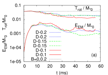
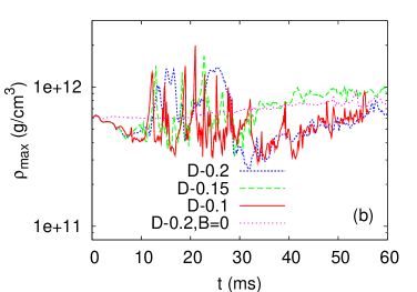
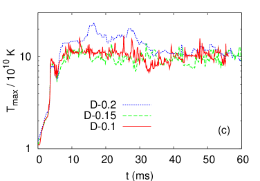
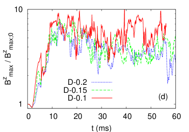
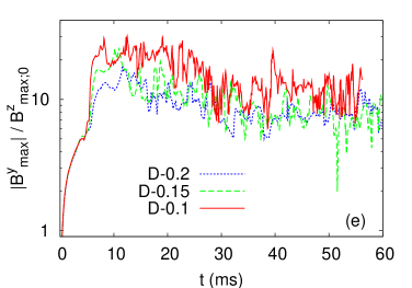
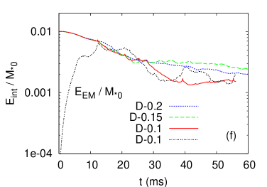
Figure 3: (a) Evolution of the rotational kinetic energy and electromagnetic energy in units of the initial value of the rest-mass, $M_{*0}$, for model D with $\Delta/M=0.1$, 0.15, and 0.2. For comparison, the results with no magnetic field and with $\Delta/M=0.2$ are also shown. (b) The same as (a), but for the maximum density. (c) The same as (a), but for the maximum temperature. (d) The same as (a), but for the maximum value of ${\cal{B}}^{z}$ in units of the initial maximum value of ${\cal{B}}^{z}$. (e) The same as (d), but for the maximum value of ${\cal{B}}^{y}$. (f) The same as (a), but for the internal energy. For comparison, the electromagnetic energy for $\Delta=0.1M$ is also shown.

Figure 3(b) plots the evolution of the maximum density. For 10 ms $\mathrel{\raise 1.29167pt\hbox{$<$}\mkern-14.0mu\lower 2.58334pt\hbox{$\sim$}}t\mathrel{\raise 1.29167pt\hbox{$<$}\mkern-14.0mu\lower 2.58334pt\hbox{$\sim$}}30$ ms, we see that it varies violently in the range between $\sim 3\times 10^{11}~{}{\rm g/cm^{3}}$ and $\sim 2\times 10^{12}~{}{\rm g/cm^{3}}$. This indicates that in such an early phase, the turbulent motion is strongly excited. For comparison, the result for the non-magnetized case is also shown. It is seen that the maximum density increases only gradually with time due to neutrino cooling, showing that the torus is approximately in a quasistationary state. This indicates that the violent time variation of the maximum density in the early phase is induced by the magnetic effects. By contrast, the maximum density gradually increases for $t\mathrel{\raise 1.29167pt\hbox{$>$}\mkern-14.0mu\lower 2.58334pt\hbox{$\sim$}}30$ ms. This is due to the fact that the rotation radius of the torus gradually decreases in the quasistationary mass accretion phase making the torus compact. [The density maximum is initially located at $\varpi\approx 10M$, whereas it is at $\varpi\approx 5M$ at $t=40$ ms; cf. Fig. 6(a)].

Because the region with $\rho\mathrel{\raise 1.29167pt\hbox{$>$}\mkern-14.0mu\lower 2.58334pt\hbox{$\sim$}}10^{11}~{}{\rm g/cm^{3}}$ is optically thick with respect to neutrinos, a fraction of the neutrinos are trapped by the matter flow, [4, 9] and this reduces the fraction of neutrinos that escape to infinity. This fact is clarified in §4.4, which displays the dependence of the neutrino luminosity on $\zeta$. The neutrino-trapping effect always plays a role for tori of mass $\mathrel{\raise 1.29167pt\hbox{$>$}\mkern-14.0mu\lower 2.58334pt\hbox{$\sim$}}0.1M_{\odot}$ in the model studied presently because $\rho_{\rm max}$ of such tori is $\geq 10^{11}~{}{\rm g/cm^{3}}$ (cf. §4.2).

Figure 3(c) plots the evolution of the maximum temperature. Because of shock heating, the temperature quickly rises in the first $\sim 10$ ms. Then, the maximum temperature reaches $\sim 10^{11}$ K and relaxes approximately to a constant value. This is a qualitatively universal feature for the tori considered in this paper. The value of the maximum temperature depends on the spin of the black hole and the mass of the torus. (cf. §4.2 and §4.3).

Figures 3(d) and (e) plot the evolution of the maximum values of $|{\cal{B}}^{z}|$ and $|{\cal{B}}^{y}|$ in units of the initial maximum value of $|{\cal{B}}^{z}|$. In the early phase, the poloidal component of the magnetic field grows in an exponential manner, indicating that the MRI occurs. By contrast, the toroidal component $|{\cal{B}}^{y}|$ increases linearly with time due to the winding of the magnetic field lines. This property is also seen in Fig. 3(a), where the electromagnetic energy increases in proportion to $t^{2}$ for $t\mathrel{\raise 1.29167pt\hbox{$<$}\mkern-14.0mu\lower 2.58334pt\hbox{$\sim$}}5$ ms. After the amplification of the magnetic field, the electromagnetic energy density becomes comparable to the internal energy density [see Fig. 3(f)]. Then the growth of the field saturates. This is also one of the universal features for the evolution of magnetized tori, irrespective of the mass of the tori and the black hole spin.

Figures 3(b)–(e) show that numerical results for the maximum density, maximum temperature, and maximum magnetic field strength do not depend strongly on the grid resolutions. This indicates that the simulation with $\Delta=0.15M$, which is a typical choice for the grid resolution, provides a result of good convergence. We note that this is also the case for any value of $a\leq 0.9M$, although higher grid resolution is required for larger values of $a$, because the coordinate radius of the event horizon is smaller in this case.

4.1.2 Evolution of accretion rates

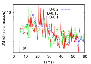
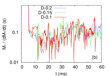
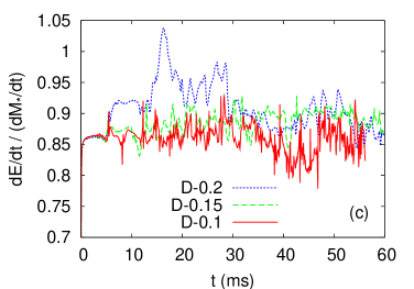
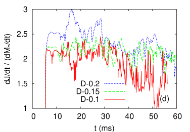
Figure 4: Evolution of (a) the rest-mass accretion rate, $\dot{M}_{*}$, (b) the accretion time scale, $M_{*}/\dot{M}_{*}$, (c) the energy accretion rate in units of the rest-mass accretion rate, $\dot{E}/\dot{M}_{*}$, and (d) the angular momentum accretion rate in units of the rest-mass accretion rate, $\dot{J}/\dot{M}_{*}$, for model D with $\Delta/M=0.1$, 0.15, and 0.2.

In Fig. 4, we plot the evolution of the rest-mass accretion rate, $\dot{M}_{*}$, accretion time scale, $M_{*}(t)/\dot{M}_{*}$, and energy and angular momentum accretion rates, $\dot{E}$ and $\dot{J}$, in units of $\dot{M}_{*}$. It is seen that as the electromagnetic energy increases [see Fig. 3(a)], the mass accretion rate quickly increases, and when the growth of the magnetic field saturates, it reaches $\sim 10M_{\odot}$/s. Then, it gradually decreases and eventually relaxes to $\sim 1$–$2M_{\odot}$/s in a quasistationary state. We note that the accretion rate depends on the mass of torus and on the black hole spin (see §4.2 and §4.3).

The associated accretion time scale for $t\mathrel{\raise 1.29167pt\hbox{$<$}\mkern-14.0mu\lower 2.58334pt\hbox{$\sim$}}30$ ms is violently time-varying with the average value of $\sim 50$ ms, but it relaxes to $\sim 0.1$–0.2 s in the quasistationary state. In a previous work [9] in which the $\alpha$-viscosity is used for the evolution of a neutrino-cooled torus of mass $\approx 0.3M_{\odot}$, the accretion time scale is $\sim 50$ ms for the $\alpha$-viscous parameter value $\alpha_{v}=0.1$ and $\sim 0.5$ s for $\alpha_{v}=0.01$. The present numerical results approximately correspond to the case that $\alpha_{v}\approx 0.1$ for the early phase and $\alpha_{v}\approx 0.04$ for the quasistationary phase. This is a universal feature for any values of the mass of the torus and the black hole spin.

The ratio of the energy accretion rate to the mass accretion rate, $\dot{E}/\dot{M}_{*}$, is $\sim 0.85$–0.9 for the high-resolution runs. One may think that this is a reasonable result, because the ratio of the specific energy to the rest-mass energy of a test particle rotating around a Kerr black hole of $a/M=0.75$ at the ISCO is $\approx 0.89$ (see Table II). However, this is an accidental coincidence, as can be understood from the following two points. (i) The torus is not composed of test particles but fluid with a significant internal energy obtained by shock heating. Due to the contribution of the specific internal energy, the value of $\dot{E}$ should increase beyond that of the test particles. (ii) The accreting matter loses kinetic energy as it falls into the black hole from the ISCO due to the magnetic stress. This effect should reduce the value of $\dot{E}$. In the present case, these two effects approximately cancel each other.

The ratio $\dot{J}/\dot{M}_{*}$ is found to be $\sim 1.5$–2.3, which is smaller than the value of the specific angular momentum for a test particle orbiting at the ISCO, $\approx 2.5$ (see Table II). This indicates that during the infall of matter into the black hole from the ISCO, the magnetic stress extracts angular momentum, which is transported outwards along the field lines, as in the case of $\dot{E}$. This effect was pointed out in Ref. MG.

4.1.3 Neutrino luminosity

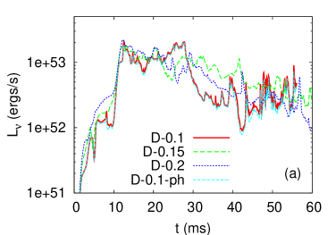
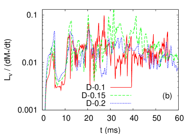
Figure 5: Evolution of (a) the neutrino luminosity, $L_{\nu}$, and (b) the efficiency of the conversion to neutrinos, $L_{\nu}/\dot{M}_{*}$, for model D with $\Delta/M=0.1$, 0.15, and 0.2. Here, “ph” denotes the result for the case that the luminosity is given by Eq. (81), which approximately overlaps with $L_{\nu}$, as the difference is less than 10%.

Figure 5 plots neutrino luminosity $L_{\nu}$ and the efficiency of the conversion to neutrinos (defined by the ratio of the neutrino luminosity to the rest-mass energy accretion rate, $L_{\nu}/\dot{M}_{*}c^{2}$). Soon after the magnetic field growth saturates at $t\sim 10$ ms, the neutrino luminosity reaches a maximum of $\sim 2\times 10^{53}$ ergs/s as a result of shock heating by violent matter motion induced by magnetic stress. Then, for 10 ms $\mathrel{\raise 1.29167pt\hbox{$<$}\mkern-14.0mu\lower 2.58334pt\hbox{$\sim$}}t\mathrel{\raise 1.29167pt\hbox{$<$}\mkern-14.0mu\lower 2.58334pt\hbox{$\sim$}}30$ ms, during which there is significant turbulent matter motion (cf. §4.1.1), it remains $\mathrel{\raise 1.29167pt\hbox{$>$}\mkern-14.0mu\lower 2.58334pt\hbox{$\sim$}}10^{53}$ ergs/s. For $t\mathrel{\raise 1.29167pt\hbox{$>$}\mkern-14.0mu\lower 2.58334pt\hbox{$\sim$}}30$ ms, the accretion rate gradually decreases, and so does the neutrino luminosity. In the quasistationary phase for $t\mathrel{\raise 1.29167pt\hbox{$>$}\mkern-14.0mu\lower 2.58334pt\hbox{$\sim$}}30$ ms, we have $L_{\nu}\sim 1$–$5\times 10^{52}$ ergs/s. As shown in subsequent sections, these values for the neutrino luminosity depends on the mass of the torus and the black hole spin.

We derive the neutrino luminosity by simply integrating the emissivity outside the event horizon. In an actual system of this kind, a fraction of the neutrinos emitted in the vicinity of black hole should be swallowed by it, because of the strong gravity. To estimate the dependence of the luminosity on the chosen domain for the integration, we also compute the luminosity, choosing the inner boundary of integration for the luminosity at $r=r_{\rm ph}$ (see the dotted curve in Fig. 5). Note that only half of the neutrinos emitted by a stationary emitter at $r=r_{\rm ph}$ can escape. In this case, the luminosity is smaller by $\sim 10\%$ than $L_{\nu}$. Thus, the real luminosity may be $\sim 90\%$ of the value of $L_{\nu}$ obtained from the integration for $r>r_{\rm H}$.

From the time integration, the total emitted neutrino energy, $\Delta E_{\nu}$, and the total accreted rest-mass for $t\leq 50$ ms are calculated, giving 3–$4\times 10^{51}$ ergs and $\sim 0.1$–$0.13M_{\odot}$ for model D. (Note that these values depend on the grid resolution.) Thus, $\sim 1.4$–2.0% of the total accreted rest-mass energy, $\Delta M_{*}c^{2}$, is converted into neutrinos. (For $\Delta/M=0.1$, 0.15, and 0.2, it is 1.6%, 2.0%, and 1.4%, respectively). The order of magnitude of this value agrees with the results presented in Refs. SRJ and LRP. Our efficiency is smaller by a factor of $\sim 2$–3 than those obtained in the previous works. This is probably because of the differences in the treatments of the gravitational fields, neutrino opacity, and angular momentum transport process. Figure 5(b) also shows that the conversion efficiency is in a narrow range (between $\sim 1\%$ and $\sim 3\%$), close to the average value of $L_{\nu}/\dot{M}_{*}c^{2}\sim 1$–2%, for the entire time.

For $a/M=0.75$, the maximum hypothetical conversion efficiency is about 11% (cf. Table II). The results here imply that the conversion efficiency is not as large as the maximum. Note that the accretion time scale, $M_{*}/\dot{M}_{*}\sim 100$ ms, is approximately as long as the neutrino emission time scale, $E_{\rm int}/L_{\nu}$. This implies that a part of the thermal energy is trapped by the matter flowing into the black hole and fails to be converted into neutrinos. Indeed, we find that the conversion efficiency depends strongly on the value of $\zeta$ (see §4.4). This is one reason for the relatively small conversion efficiency. Another reason is that the initial radius of the torus is $\approx 10M$ at the density maximum and at most $30M$ in the present model. The difference between the specific binding energy at $r=10M$ and at the ISCO is $\approx 6\%$, and hence much smaller than 11%. We note that the radii of the ISCO are larger for smaller values of the black hole spin. Thus, the conversion efficiency is even suppressed for smaller values of the black hole spin, as shown in §4.3. On the other hand, the suppression factor for larger spin with $a/M=0.9$ is smaller.

Numerical simulations indicate that the formation of a black hole-torus system from stellar core collapse and the merger of a black hole and neutron star is divided into two stages [e.g., Refs. GRB0,Proga,SS07,BHNS0,BHNS1,SU06]. In the first stage, the black hole and accretion torus are formed dynamically. According to our present numerical results, in such a stage, the amplification of magnetic fields and the subsequent redistribution of angular momentum proceed violently in the presence of magnetic fields of appreciable magnitude. As a result, shocks are generated, increasing the temperature of the torus, and the neutrino luminosity thereby reaches $\mathrel{\raise 1.29167pt\hbox{$>$}\mkern-14.0mu\lower 2.58334pt\hbox{$\sim$}}10^{53}$ ergs/s. In the second stage, the system relaxes to a quasistationary state. In such a stage, the mass and spin of the black hole become approximately constant and the accretion proceeds with a time scale longer than that of the first stage. The present numerical results indicate that for this stage, the neutrino luminosity is of order $10^{52}$ ergs/s.

A characteristic feature found in the MHD simulation is that the luminosity curve is not smooth, in contrast to that reported in Refs. SRJ and LRP. This is due to the fact that in the present simulation, shock heating is associated with turbulent (i.e. irregular) matter motion driven by highly variable magnetic stress, whereas in the previous simulations, the heating is induced by $\alpha$-viscosity, which leads to a nearly stationary accretion.

The light curve of GRBs is often not smooth.[1] If the GRBs are driven by pair annihilation of neutrino-antineutrino pairs emitted from the torus [1], the luminosity curve of neutrinos should also be highly variable. The scenario in which the original thermal source of neutrinos is attributed to shock heating driven by the chaotic magnetic activity is thus favorable.

The luminosity and total emitted neutrino energy, $\Delta E_{\nu}$, do not depend strongly on the grid resolution for $a/M\leq 0.75$. (The values of $\Delta E_{\nu}$ for $\Delta/M=0.15$ and 0.2 agree within $\sim 10$–20%; cf. Table III.) This indicates that for computing the luminosity, a grid resolution with $\Delta=0.2M$ is acceptable for $a\leq 0.75M$. By contrast, for $a=0.9M$, the luminosity and total energy for $\Delta/M=0.15$ and 0.2 do not agree well. (The relative error is by 20–30%; cf. Table III.) The reason for this difference is that the radius of the ISCO is much smaller than in the other models. (The ISCO is located at $\varpi\approx 2.5M$; cf. Table II.) Because a large fraction of neutrinos are emitted near the ISCO, the luminosity depends strongly on the resolution near there. For $a\geq 0.9M$, a grid resolution with $\Delta=0.2M$ is not acceptable for obtaining a result with good convergence. For $a=0.9M$, we performed a simulation with $\Delta=0.12M$ and found that the results with $\Delta=0.15M$ are in good agreement with those with $\Delta=0.12M$. This indicates that a grid resolution of $\Delta=0.15M$ is acceptable even for $a=0.9M$.

4.1.4 Structure of the torus in the quasistationary phase

(a)

(b)

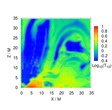
(c)

(d)

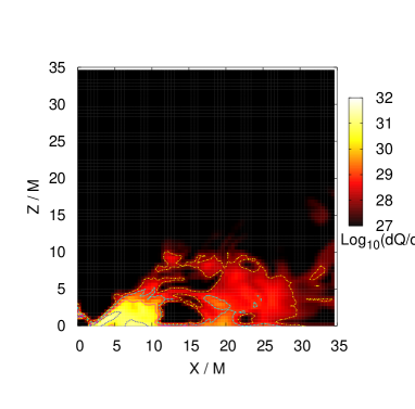
(e)

(f)

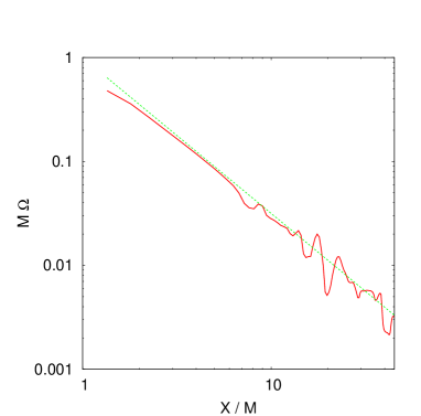
Figure 6: Color plots for (a) the density, (b) the temperature, (c) the electron fraction, (d) the neutrino emissivity, and (e) the ratio of the magnetic pressure to the gas pressure at $t\approx 40$ ms for model D with $\Delta/M=0.15$. For (d), the region with $\dot{Q}<10^{27}~{}{\rm ergs/s/cm^{3}}$ is shaded black. The contour curves are plotted for (a) $\rho=10^{8+i}~{}{\rm g/cm^{3}}~{}(i=0$–3), (b) $\log(T_{10})=0$, 0.4, and 0.8, (c) $Y_{e}=0.1\times i~{}(i=1$–5, (d) $\dot{Q}=10^{28+i}~{}{\rm ergs/s/cm^{3}}~{}(i=0,3)$, and (e) $P_{\rm mag}/P=10^{-2+2i}~{}(i=0$–2). (f) The angular velocity as a function of the cylindrical radius on the equatorial plane (solid curve). The dotted line denotes $M\Omega=(M/\varpi)^{3/2}$. Note that $M\approx 5.9$ km in the geometrical units.

In Fig. 6, we display color plots and contour curves for the density, temperature, electron fraction, neutrino emissivity, and ratio of the magnetic pressure to the gas pressure at $t\approx 40$ ms for model D. At $t=40$ ms, the accretion torus relaxes to an approximately quasistationary state. The density maximum of the torus with $\rho_{\rm max}\sim 10^{12}~{}{\rm g/cm^{3}}$ is located at $\varpi\approx 5M$ on the equatorial plane. Only a small part of the inner region with $\varpi\mathrel{\raise 1.29167pt\hbox{$<$}\mkern-14.0mu\lower 2.58334pt\hbox{$\sim$}}10M$ and with $|z|\mathrel{\raise 1.29167pt\hbox{$<$}\mkern-14.0mu\lower 2.58334pt\hbox{$\sim$}}2M$ has a density larger than $10^{11}~{}{\rm g/cm^{3}}$ and is optically thick. The temperature is also highest, $\sim 10^{11}$ K, for this high-density region, because the cooling is not efficient for such a region, due to its high opacity . The temperature of the optically thin region with $\rho<10^{11}~{}{\rm g/cm^{3}}$ is $\sim 3\times 10^{10}$ K near the equatorial plane. An interesting feature is that the temperature is not uniformly low in the region above the torus. The reason for this is that the magnetic stress in the torus induces an outflow which ejects gas with high temperature. This dilute gas subsequently emits neutrinos, and the temperature thereby quickly decreases.

As reported in Ref. LRP, the electron fraction inside the torus is low, $\mathrel{\raise 1.29167pt\hbox{$<$}\mkern-14.0mu\lower 2.58334pt\hbox{$\sim$}}0.1$. This reflects the fact that the density is so high that the electrons are highly degenerate. A typical value of the degeneracy parameter is $\eta_{e}\sim 2$–4 in the region with $\rho\mathrel{\raise 1.29167pt\hbox{$>$}\mkern-14.0mu\lower 2.58334pt\hbox{$\sim$}}10^{11}~{}{\rm g/cm^{3}}$. Around the envelope of the torus in the low density region ($\rho\mathrel{\raise 1.29167pt\hbox{$<$}\mkern-14.0mu\lower 2.58334pt\hbox{$\sim$}}10^{9}~{}{\rm g/cm^{3}}$), by contrast, the degeneracy is low, with $\eta_{e}<1$ for a large fraction of the fluid.

Neutrinos are efficiently emitted in the region satisfying $\varpi\mathrel{\raise 1.29167pt\hbox{$<$}\mkern-14.0mu\lower 2.58334pt\hbox{$\sim$}}10M$ and $|z|\mathrel{\raise 1.29167pt\hbox{$<$}\mkern-14.0mu\lower 2.58334pt\hbox{$\sim$}}5M$. The neutrino emissivity is highest near the surface of the torus (not at the density maximum), because the region in the vicinity of the density maximum is so dense that the neutrinos cannot escape. In particular, the region near the inner edge of the torus has high emissivity. A large fraction of the neutrinos emitted from there will propagate toward the symmetry axis, where the neutrinos can escape freely, and hence, the pair annihilation rate of neutrinos and antineutorinos is expected to be highest in the vicinity and around the symmetry axis of a rotating black hole.

The distribution of $P_{\rm mag}/P$ exhibits a clear contrast. In the torus, the value of $P_{\rm mag}/P$ is much smaller than unity, implying that the gas pressure is dominant. By contrast, the value near the symmetry axis is much larger than unity, and hence, the gas pressure is negligible there. This structure has already been found in previous GRMHD simulations with a simple $\Gamma$-law EOS [17, 18]. The present results show that the formation of such a distribution of $P_{\rm mag}/P$ does not depend on the EOS and the neutrino cooling.

Figure 6(f) plots the angular velocity along the cylindrical radius in the equatorial plane. This illustrates that the velocity of the torus is approximately Keplerian in the quasistationary phase. At the beginning of the simulation, the profile of the angular velocity is steeper than this, as shown in Fig. 2. Due to the magnetic braking and the MRI, the angular momentum is redistributed, and the profile of the angular velocity is modified and becomes Keplerian. The resulting torus is likely to be stable with respect to nonaxisymmetric instabilities and the runaway instability because of the Keplerian velocity profile.

4.2 Dependence on the mass and the initial radius of the torus

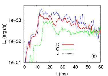
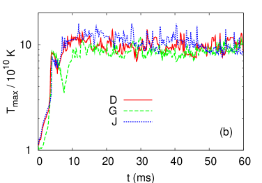
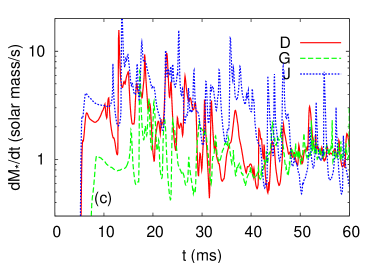
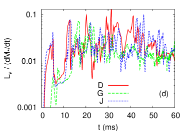
Figure 7: Evolution of (a) the neutrino luminosity, (b) the maximum temperature, (c) the mass accretion rate, and (d) the efficiency of the conversion to neutrinos $L_{\nu}/\dot{M}_{*}$, for models D, G, and J with $\Delta/M=0.15$. Because the initial rotation radii are slightly larger, the luminosity and temperature for model G rise at slightly later time than for other models.

In Fig. 7(a), we plot the neutrino luminosity as a function of time for models D, G, and J. The mass of torus varies among these models, while the spin parameter of the black hole is the same and the initial rotation radii of the torus are approximately equal at $t=0$. Figure 7(a) shows that the luminosity systematically increases as the mass of the torus increases. This is simply due to the fact that there are more emitters for the larger-mass models. Because the maximum density is slightly higher (see Table I), there should be more trapped neutrinos for the larger-mass models, suppressing the neutrino luminosity. However, this does not decrease the neutrino luminosity significantly. The temperature is slightly higher for the larger-mass models [see Fig. 7(b)]. This is one reason that the neutrino luminosity increases with the torus mass.

The mass accretion rate is larger for the larger-mass models in the early phase, i.e., for $t\mathrel{\raise 1.29167pt\hbox{$<$}\mkern-14.0mu\lower 2.58334pt\hbox{$\sim$}}40$ ms [see Fig. 7(c)]. As a result, at late times ($t\mathrel{\raise 1.29167pt\hbox{$>$}\mkern-14.0mu\lower 2.58334pt\hbox{$\sim$}}40$ ms), the differences among the mass accretion rates of the three models are relatively small, resulting in relatively small differences among the neutrino luminosities. The authors of Ref. SRJ report that the neutrino luminosity is approximately proportional to $M_{*}$ for the case of nonzero $\alpha$-viscosity. In the present result, the maximum luminosity and total energy carried by neutrinos are approximately proportional to $M_{*}$.

Figure 7(d) plots the conversion efficiency, $L_{\nu}/\dot{M}_{*}$, as a function of time for models D, G, and J. Although the neutrino luminosity differs significantly among three models, the conversion efficiency, varying between $\sim 1$% and $\sim 5\%$, does not depend on the mass of the torus as strongly as the luminosity. The average conversion efficiency, $\Delta E_{\nu}/\Delta M_{*}$, is also in a narrow range between 1.4% and 1.8% for models G–J (see Table III).

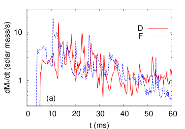
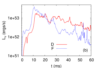
Figure 8: Evolution of (a) the mass accretion rate, $\dot{M}_{*}$, and (b) the neutrino luminosity, $L_{\nu}$, for models D and F with $\Delta/M=0.15$.

To see the dependence of the rest-mass accretion rate and neutrino luminosity on the initial radius of the torus, we performed a simulation for model F. This model has the same black hole spin and approximately the same torus rest-mass as model D, but it has a smaller initial rotation radius. In Fig. 8, we plot the mass accretion rate and the neutrino luminosity for models D and F. Because model F has a smaller radius initially, the mass accretion rate and the neutrino luminosity quickly increase at earlier times. Also, the peak value of the luminosity for model F is larger by a factor of $\sim 2$ than that for model D, whereas the luminosity at late times is smaller for model F. However, the total emitted neutrino energy and the efficiency of the conversion to neutrinos are similar (see Table III).

4.3 Dependence on the black hole spin

Figure 9 plots the mass accretion rate and the neutrino luminosity as functions of time for models B–E. The black hole spin is different for each of these models, but the mass and rotation radii of the torus are approximately equal at $t=0$. We find the following. (i) The luminosity for model E is largest among the four models, whereas the mass accretion rate is smallest for model E, probably because its event horizon has the smallest area. (ii) The luminosity increases with $a$ by a significant amount only for $a\geq 0.5M$ (see also Table III). The magnitude of the luminosity varies only slightly for $a/M=0$–0.5, while the luminosities for models B and C are approximately the same. (iii) The decay time of the luminosity increases with $a$ for $a/M\geq 0.5$. The facts (i)–(iii) indicate that for a sufficiently large value of the spin, $a\mathrel{\raise 1.29167pt\hbox{$>$}\mkern-14.0mu\lower 2.58334pt\hbox{$\sim$}}0.75M$, the effect of the black hole spin enhances the neutrino luminosity, but for smaller values, the luminosity is not significantly enhanced by the spin effect. In the following, we describe the reasons for these types of behaviors.

There are two factors which determine the dependence of the luminosity on the black hole spin. One is the fact that with larger spin, the radius of the ISCO decreases as the spin increases (cf. Table II). Then, the gravitational binding energy at the ISCO ($1-E_{\rm ISCO}$), which could be converted to thermal energy, increases as a function of $a$ (cf. Table II). Indeed, the maximum temperature also increases as $a$ increases [see Fig. 10(a)]. This results in an enhancement of the efficiency for converting gravitational binding energy into neutrinos. Note that the gravitational binding energy at the ISCO changes slowly as a function of $a$ for small values of $a$. This implies that this effect is not very important for $a\ll M$.

The small radii of the ISCO for larger values of the spin also result in the decrease of the mass accretion rate and in the increase of the accretion time. To achieve a high neutrino luminosity, a longer accretion time is favorable, because a fraction of the thermal energy trapped with the matter flowing into black hole is reduced. Thus, the case of a large spin has an advantage with regard to enhancing the neutrino luminosity due to (i) the large binding energy at the ISCO and (ii) the long accretion time.

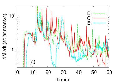
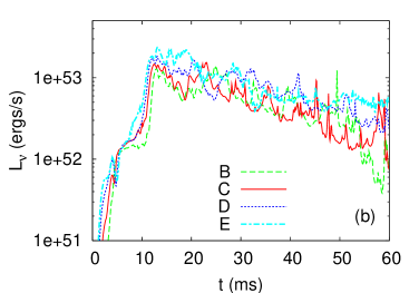
Figure 9: Evolution of (a) the mass accretion rate for models B, C, and E with $\Delta/M=0.15$. (b) the neutrino luminosity, $L_{\nu}$, for models B, C, D, and E with $\Delta/M=0.15$.

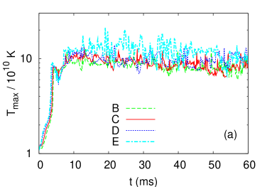
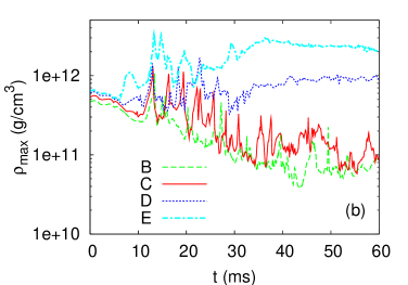
Figure 10: Evolution of the maximum temperature, $T_{\rm max}$, and density, $\rho_{\rm max}$, for models B–E with $\Delta/M=0.15$.

The other factor is that for a larger value of $a$, the rotation radius of the torus can be smaller. This results in a more compact torus which has a higher temperature and larger density. As a result of the larger density, (i) the trapped fraction of neutrinos is increased, whereas (ii) the neutrino luminosity could be increased because of the higher temperature and larger density. Figure 10 plots the evolution of the maximum temperature and density for models B–E. For model B, the maximum density gradually decreases below $10^{11}~{}{\rm g/cm^{3}}$, which implies that no trapped neutrinos exist in the late phase. For model C, $\rho_{\rm max}$ is slightly larger than $10^{11}~{}{\rm g/cm^{3}}$, and hence, a small fraction of neutrinos are trapped. For models D and E, in which $\rho_{\rm max}\sim 10^{12}~{}{\rm/cm^{3}}$, a large fraction of neutrinos are trapped, whereas the emissivity is enhanced by the large density.

For models B and C, the above two factors seem to play an accidently identical role, resulting in similar luminosities. For models D and E, on the other hand, the enhancement of the luminosity at high temperature and high density plays a stronger role than the effect of the opacity. Because the luminosity for models D and E is much larger than for models A–C, the longer accretion time and high temperature resulting from the large spin play the most significant role in enhancing the luminosity.

In the present numerical work, there is the additional reason that the conversion efficiency increases rapidly with the spin for $a/M\mathrel{\raise 1.29167pt\hbox{$>$}\mkern-14.0mu\lower 2.58334pt\hbox{$\sim$}}0.75$. As mentioned above, the radius of the ISCO for black holes of larger spins is smaller, and a larger fraction of the rest-mass energy can be converted into thermal energy (cf. Table II). In the present model, the density maximum for the torus is initially located at $\sim 10M$. For smaller values of the spin, then, the possible conversion rate for matter near the density maximum is much smaller than the maximum allowed value given in Table II, because the difference between the specific binding energy at the ISCO and at the density maximum is much smaller than the specific binding energy at the ISCO. For large values of the spin with $a\rightarrow M$, by contrast, the difference is close to the specific binding energy at the ISCO. This is one reason that the conversion efficiency for models D and E is much larger than those for other models.

4.4 Dependence on $\zeta$

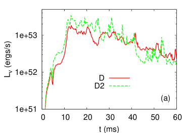
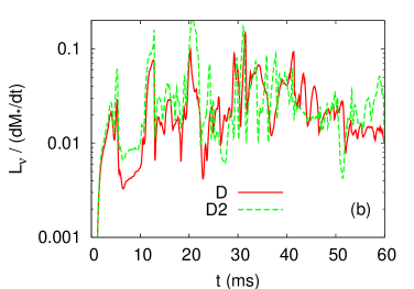
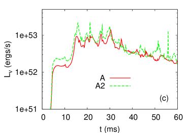
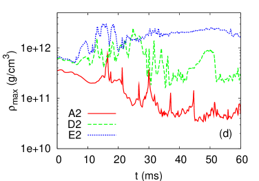
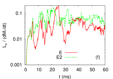
Figure 11: Evolution of (a) the neutrino luminosity, $L_{\nu}$, and (b) the efficiency of the conversion to neutrinos, $L_{\nu}/\dot{M}_{*}$, for models D and D2 with $\Delta/M=0.15$. (c) The same as (a), but for models A and A2 with $\Delta/M=0.2$. (d) Evolution of the maximum density for models A2, D2, and E2. (e) The same as (a), but for models E and E2 with $\Delta/M=0.15$. (f) The same as (b) but for models E and E2 with $\Delta/M=0.15$.

In this subsection, we compare the results for pair models for which the black hole spin and properties of the torus are identical but the rule for identifying the optically thick region for neutrinos is different. We determine that the region with $\rho_{11}\geq 1$ is optically thick for models A–E, whereas the region with $\rho_{11}\geq 3$ is for models A2–E2.

Figure 11(a) plots the evolution of the neutrino luminosity, $L_{\nu}$, and the conversion efficiency, $L_{\nu}/\dot{M}_{*}$, for models D and D2. Because the optically thin region is wider, the neutrino luminosity for model D2 is higher than that for model D, in particular in the early phase, with $t\mathrel{\raise 1.29167pt\hbox{$<$}\mkern-14.0mu\lower 2.58334pt\hbox{$\sim$}}30$ ms. The relative difference is $\sim 30$–40%.

The conversion efficiency, $L_{\nu}/\dot{M}_{*}$, for model D2 is larger than that for model D, reflecting the higher luminosity for model D2. It often reaches 10% and is $\sim 2.5\%(\sim\Delta E_{\nu}/\Delta M_{*}c^{2}$) on average. Nevertheless, it is smaller than the maximum value, $\sim 11\%$. Recalling that the accretion time scale, $M_{*}/\dot{M}_{*}\sim 100$ ms, is approximately as long as the neutrino emission time scale, $E_{\rm int}/L_{\nu}$, this implies that a large fraction of the neutrinos are still trapped by the matter and advected into the black hole, thus failing to escape from the torus. Indeed, the maximum density for model D2 is larger than $3\times 10^{11}~{}{\rm g/cm^{3}}$ for most of the time [see Fig. 11(d)].

Figure 11(c) plots the evolution of the neutrino luminosity for models A and A2. As in models D and D2, the luminosity for model A2 is larger than that for model A. However, the difference is not as large as that between models D and D2. The reason for this smaller difference is that the density of the torus for models A and A2 is not as large as that for models D and D2 [see Figs. 10(b) and 11(d)]. In particular, for $t\mathrel{\raise 1.29167pt\hbox{$>$}\mkern-14.0mu\lower 2.58334pt\hbox{$\sim$}}20$ ms, the density is smaller than $10^{11}~{}{\rm g/cm^{3}}$, and hence, no region is optically thick for models A and A2. We conclude that for a torus with small values of $a$ and with mass $\approx 0.25M_{\odot}$, the neutrino luminosity depends only weakly on the value of $\zeta~{}(\mathrel{\raise 1.29167pt\hbox{$>$}\mkern-14.0mu\lower 2.58334pt\hbox{$\sim$}}1/3)$.

The same conclusion is reached for tori of small mass which would have densities smaller than $10^{11}~{}{\rm g/cm^{3}}$. (Compare the maximum densities for models D, F–J in Table I.) Actually, only a small fraction of a torus with $M_{*}\mathrel{\raise 1.29167pt\hbox{$<$}\mkern-14.0mu\lower 2.58334pt\hbox{$\sim$}}0.1M_{\odot}$ is optically thick for $a\leq 0.75M$. For $a\sim 0$, the neutrino-trapping effect plays an important role only for massive tori with $M_{*}\mathrel{\raise 1.29167pt\hbox{$>$}\mkern-14.0mu\lower 2.58334pt\hbox{$\sim$}}0.3M_{\odot}$. For large values of $a$, i.e., for $a\mathrel{\raise 1.29167pt\hbox{$>$}\mkern-14.0mu\lower 2.58334pt\hbox{$\sim$}}0.75M$, by contrast, neutrino trapping plays a role even for $M_{*}\sim 0.1M_{\odot}$.

In Fig. 11(e), we plot the evolution of the neutrino luminosity for models E and E2. In contrast to the results for $a\leq 0.75M$, the luminosities for $\zeta=1$ and 1/3 differ significantly. The reasons are that (i) for $a=0.9M$, the rotation radii of the torus can be small enough ($\varpi\sim 2.5M$; see Table II) to constitute a compact torus and that (ii) the accretion time scale is long enough to halt quick accretion for large-spin black holes. Consequently, the density can increase to $\mathrel{\raise 1.29167pt\hbox{$>$}\mkern-14.0mu\lower 2.58334pt\hbox{$\sim$}}10^{12}~{}{\rm g/cm^{3}}$ even with $M\approx 0.25M_{\odot}$ [see Fig. 10(b)]. Because the optically thick region is large for such accretion flow, the decrease of $\zeta$ significantly increases the size of the optically thin region and the luminosity.

In Fig. 11(f), the evolution of the conversion efficiency, $L_{\nu}/\dot{M}_{*}$, is plotted for models E and E2. It is seen that the conversion efficiency for model E2 is about 2.5 times as large as that for E. For $a=0.9M$, the hypothetical maximum conversion efficiency is about 15.5% (cf. Table II). For model E2, the average conversion efficiency ($\Delta E_{\nu}/\Delta M_{*}$) is $\sim 6\%$, which is thus $\sim 40\%$ of the maximum value. For $a\sim M$, approximately $40\%$ of the rest-mass energy may be converted into thermal energy. [27] Our results for model E2 suggest that a conversion efficiency of $\sim 20\%$ may be possible for $a\sim M$.

We determine the neutrino optical depth in a simple qualitative way, using the local density. In an actual system, the optical depth depends on the density distribution, temperature profile, neutrino energy, geometry of the black hole, and path of neutrinos in the curved geometry. Although the assumption $\tau_{\nu}=\zeta\rho_{11}$ is not bad qualitatively, the error is not small quantitatively: Comparing the results for $\zeta=1$ and $1/3$, we infer that the error in the luminosity is approximately a factor of 2–3 for large values of the black hole spin. To obtain the neutrino luminosity more accurately, it is necessary to adopt a more sophisticated method for determining the optical depth, in particular for large values of $a$. This is beyond scope of this paper and left for future study.

5 Summary and discussion

5.1 Summary

We have reported our first numerical results of a GRMHD simulation for neutrino-cooled accretion tori. We solved the GRMHD equations in the fixed gravitational field of Kerr black holes of mass $4M_{\odot}$ with a realistic EOS and with neutrino cooling. The simulation was carried out systematically for a wide range of values of the black hole spin and the torus mass. Below we summarize the results of the numerical simulation.

• In the presence of both poloidal magnetic fields and differential rotation, the magnetic field strength is amplified by the winding of the field lines and by the MRI until the electromagnetic energy reaches $\sim 10\%$ of the rotational kinetic energy. Then, the magnetic stress induces angular momentum transport via magnetic braking and the MRI, resulting in a quasistationary accretion onto the black hole. It also drives turbulent motion of matter, which subsequently generates shocks that convert kinetic energy into thermal energy. Through these processes, the temperature of the torus increases typically to $\sim 10^{11}$ K. The ratio of the electromagnetic energy to the rotational kinetic energy is maintained at $\sim 10\%$ in the quasistationary accretion phase. This electromagnetic energy is comparable to the internal energy in the quasistationary phase.

• The maximum density of the torus takes values in a wide range, between $\sim 10^{10}~{}{\rm g/cm^{3}}$ and $\sim 10^{12}~{}{\rm g/cm^{3}}$, depending on black hole spin $a$ and mass of the torus $M_{*}$. For larger values of $a$, the maximum density tends to be higher for a given value of $M_{*}$, because (i) the location of the ISCO is closer to the horizon, leading to a more compact torus, and (ii) the accretion rate is suppressed by the small ISCO radius, halting the infall of the matter and resulting in the formation of a higher-density region near the ISCO. For a larger torus mass, the maximum density becomes larger.

• In the case that the density is sufficiently high, some of the neutrinos are trapped in the accretion flow, which suppresses the neutrino emission rate. This tends to happen for large values of $a$ and for large values of the torus mass.

• Before the torus relaxes to a quasistationary state, the accretion rate reaches $\sim 10M_{\odot}$ /s, but after it relaxes, a typical accretion rate is $\sim M_{\odot}$ /s. The corresponding accretion time scale is $\sim 50$ ms in the early phase, but it relaxes to 100–200 ms in the quasistationary state. This accretion rate is in agreement with that in the case that an $\alpha$-viscosity in the range $\alpha_{v}=0.01$–0.1 is included.

• The maximum neutrino luminosity is a few $\times 10^{53}$ ergs/s for the torus mass $M_{*}\approx 0.25M_{\odot}$, irrespective of the value of the black hole spin for $0\leq a/M\leq 0.9$. (For $a=0.9M$ and $\zeta=1/3$, the maximum reaches exceptionally $10^{54}$ ergs/s.) In the quasistationary phase, it is between $10^{52}$ ergs/s and $10^{53}$ ergs/s, which depends strongly on the black hole spin. The efficiency of the conversion to neutrinos, $L_{\nu}/\dot{M}_{*}$, is between 1 and 10 %. This value depends on the black hole spin and the effect of neutrino trapping. The total emitted neutrino energy is $2\times 10^{51}$–$2\times 10^{52}$ ergs for $M_{*}\approx 0.25M_{\odot}$. This also depends strongly on the black hole spin and the effect of neutrino trapping.

• The neutrino luminosity, $L_{\nu}$, and the total emitted neutrino energy depend strongly on the mass of the torus, $M_{*}$. The maximum value of the luminosity and the total emitted energy are approximately proportional to $M_{*}$ for $M_{*}\mathrel{\raise 1.29167pt\hbox{$<$}\mkern-14.0mu\lower 2.58334pt\hbox{$\sim$}}0.4M_{\odot}$.

• Neutrinos are emitted efficiently in the region with $\varpi\mathrel{\raise 1.29167pt\hbox{$<$}\mkern-14.0mu\lower 2.58334pt\hbox{$\sim$}}10M$ and $|z|\mathrel{\raise 1.29167pt\hbox{$<$}\mkern-14.0mu\lower 2.58334pt\hbox{$\sim$}}5M$. In particular, the neutrino emissivity is highest near the inner surface of the accreting torus.

• The neutrino luminosity and the conversion efficiency for $a\mathrel{\raise 1.29167pt\hbox{$>$}\mkern-14.0mu\lower 2.58334pt\hbox{$\sim$}}0.75M$ are larger by a factor of $\mathrel{\raise 1.29167pt\hbox{$>$}\mkern-14.0mu\lower 2.58334pt\hbox{$\sim$}}2$ than those for $a=0$. However, moderate values of the spin ($a\mathrel{\raise 1.29167pt\hbox{$<$}\mkern-14.0mu\lower 2.58334pt\hbox{$\sim$}}0.5M$) do not help to significantly increase the luminosity for a torus of mass $M_{*}=0.1$–0.4$M_{\odot}$.

• If the accretion flow is optically thin with respect to neutrino transport, the efficiency of the conversion to neutrinos may be larger than $\sim 10\%$ for $a\mathrel{\raise 1.29167pt\hbox{$>$}\mkern-14.0mu\lower 2.58334pt\hbox{$\sim$}}0.9M$.

5.2 Implications for GRBs

Because neutrinos are emitted most efficiently near the inner surface of accreting torus, neutrino-antineutrino pair annihilation is expected to occur in the vicinity of the rotation axis of black hole. As a result, a pair plasma of electrons and positrons may be generated, forming a fireball near the rotation axis. If the energy density of this fireball is sufficiently high, it can drive GRBs.[1] Setiawan et al. [8] estimated the luminosity of gamma rays, and found that it could be $E_{\nu\bar{\nu}}\sim 10^{50}$–$10^{51}$ ergs/s for $L_{\nu}\sim 10^{53}$ ergs/s. Such a large value would be sufficiently high to generate GRBs if the total baryon mass in the vicinity of the rotation axis is sufficiently small. [44] We find that the neutrino luminosity is $\sim 10^{53}$ ergs/s for a torus mass of $\mathrel{\raise 1.29167pt\hbox{$>$}\mkern-14.0mu\lower 2.58334pt\hbox{$\sim$}}0.2M_{\odot}$ and black hole mass of $4M_{\odot}$, irrespective of the black hole spin. It is believed that such a system may act as the central engine of GRBs (specifically, GRBs of short duration). In particular, for large values of $a$ close to unity, the efficiency of the conversion to neutrinos could be high, and a strong GRB would then be driven.

In our present treatment, the heating of matter by neutrinos emitted from the torus and neutrino-antineutrino pair annihilation are not taken into account. In an actual system, neutrino heating will help the formation of matter outflow, which will contribute to sweeping baryons around the rotation axis.

The neutrino luminosity decreases as a function of the torus mass. For a torus of mass $\sim 10^{-2}M_{\odot}$, the luminosity is likely to be at most $\sim 10^{52}$ ergs/s. Because the pair annihilation rate of a neutrino-antineutrino process is proportional to the square of the neutrino luminosity, $E_{\nu\bar{\nu}}$ is likely to be $\mathrel{\raise 1.29167pt\hbox{$<$}\mkern-14.0mu\lower 2.58334pt\hbox{$\sim$}}10^{49}$ ergs/s, and hence, tori of small mass are unlikely to drive the observed GRBs. Numerical simulations have shown that the merger of binary neutron stars of sufficiently large mass can produce a system consisting of a rotating black hole and a torus of spin $a/M=0.7$–0.8 (e.g., Refs. STU,OJ). However, the torus mass is in general small, $\ll 0.1M_{\odot}$, unless the mass ratio of the two neutron stars is sufficiently small, $\mathrel{\raise 1.29167pt\hbox{$<$}\mkern-14.0mu\lower 2.58334pt\hbox{$\sim$}}0.7$–0.8. Even for a small mass ratio of $\sim 2/3$, the torus mass is at most $\sim 0.1M_{\odot}$. This indicates that the merger of binary neutron stars with sufficiently large total mass could result only in weak GRBs in most cases. If the total mass of binary neutron stars is not large enough for the direct formation of a black hole, a hypermassive neutron star is formed.[45] (See Ref. BSS for the definition of the hypermassive neutron star.) If it is strongly magnetized, such a hypermassive neutron star will collapse and become a rotating black hole with a massive torus, due to the transport of angular momentum induced by magnetic effects. [13] It is believed that the resulting system of a black hole and a torus may be the central engine of GRBs, in contrast to the case that the total mass of the binary neutron stars is large enough for the direct formation of black hole. Another possibility as the source of GRBs is the merger of black holes and neutron stars. If the mass of the black hole is not large ($\mathrel{\raise 1.29167pt\hbox{$<$}\mkern-14.0mu\lower 2.58334pt\hbox{$\sim$}}4M_{\odot}$), the resulting mass of the torus around the black hole can be $\mathrel{\raise 1.29167pt\hbox{$>$}\mkern-14.0mu\lower 2.58334pt\hbox{$\sim$}}0.1M_{\odot}$. [31, 32, 33] Therefore, it is regarded as a strong possibility as the source of GRBs.

A characteristic feature found in the MHD simulation is that the luminosity varies on a short time scale of a few ms, in contrast to the results reported in Refs. SRJ and LRP. This is due to the fact that shock heating in the magnetized accretion torus is associated with turbulent matter motion driven by a highly variable magnetic stress. The light curve of GRBs is often highly variable.[1] If the GRBs are driven by pair annihilation of neutrino-antineutrino pairs emitted from the magnetized torus [1], the luminosity curve of neutrinos should also be highly variable. Thus, the light curve of GRBs may be naturally explained if the central engine is composed of a rotating black hole and a magnetized accretion torus of mass $\mathrel{\raise 1.29167pt\hbox{$>$}\mkern-14.0mu\lower 2.58334pt\hbox{$\sim$}}0.1M_{\odot}$.

5.3 Future tasks

This work is the first step toward obtaining a detailed understanding of the evolution of dense, hot magnetized tori surrounding a stellar-mass black hole. There are several tasks left for the future. One is to take into account more realistic microphysics, incorporating more sophisticated EOSs. To this time, two tabulated finite-temperature EOSs have been published for public use. These incorporate the effects of heavy nuclei as well as free nucleons and $\alpha$-particles. [10, 48] In these EOSs, the pressure, internal energy, and other various quantities are written as functions of the density, electron fraction, and temperature, like the EOS used in this paper. Thus, it would be straightforward to change the numerical code to use more realistic tabulated EOSs. Numerical results, such as the rest-mass accretion rate, temperature, and neutrino luminosity, may depend on the chosen EOSs. To clarify this dependence, we plan to perform simulations with such EOSs.

Another task is to improve the scheme for treating neutrino transfer. As pointed out in Refs. GRB1,GRB2,GRB3,SRJ and LRP and reconfirmed in this paper, the luminosity is significantly affected by neutrino-trapping effects. In this paper, we determined the neutrino optical depth by simply using the local density. However, the actual optical depth depends on the density distribution, temperature profile, neutrino energy, and geometry of the black hole. As shown in §4.4, the luminosity depends strongly on the chosen optical depth for large values of $a$ and $M_{*}$, because such tori are composed both of optically thick and thin regions. To provide a better estimate of the neutrino luminosity, we have to treat the optical depth more carefully.

Elucidating the exact neutrino trajectories in the curved spacetime is also an important problem. Neutrinos are most efficiently emitted in the vicinity of the black hole. This implies that a non-negligible fraction is swallowed by the black hole due to large curvature effects. We plan to study this effect in the future. An associated problem is to estimate the annihilation rate of neutrino and antineutrino pairs. As mentioned above, this process generates a pair plasma for GRBs. Although Setiawan et al. already calculated this rate in their simulation,[8] they did not take into account the curvature effect. We consider that estimating the energy generation rate in curved spacetime is an important problem.

The final problem that warrants further study concerns nonaxisymmetric effects. The development of the MRI in an axisymmetric system could be different from that in the nonaxisymmetric, 3D case.[49] Turbulence tends to persist more in the 3D case due to the lack of symmetry. Specifically, according to the axisymmetric anti-dynamo theorem,[50] the sustained growth of magnetic field energy is not possible through axisymmetric turbulence, as demonstrated by numerical simulations.[51] In our present simulation, we found that the neutrino luminosity decreases with a time scale of $\sim 100$ ms, implying that the efficiency of shock heating in the torus decreases with time. This may be partly due the anti-dynamo effect. McKinney and Gammie [17] have performed axisymmetric simulations of magnetized tori accreting onto Kerr black holes and have found good quantitative agreement with the 3D results of De Villiers and Hawley [52] for the global quantities $\dot{E}/\dot{M}_{*}$ and $\dot{J}/\dot{M}_{*}$ for $t\leq 2000M$. Thus, the results presented here likely provide (at least) a good qualitative picture at least for the short-term evolution. However, to clarify the longer-term evolution, 3D simulations will eventually be necessary.

Appendix A Derivation of the equation for $T_{\mu\nu}$

The total energy-momentum tensor, $T^{\rm T}_{\mu\nu}$, is defined by the sum of energy momenta of all the matter fields, and obeys the conservation equation

$$\nabla^{\mu}T^{\rm T}_{\mu\nu}=0.$$ (106)

In the context of the present paper, $T^{\rm T}_{\mu\nu}$ is composed of the energy momenta of baryons, electrons, positrons, radiation, and neutrinos. Then, we split the total energy-momentum tensor as

$$T^{\rm T}_{\mu\nu}=T_{\mu\nu}+T^{\rm N}_{\mu\nu},$$ (107)

where $T_{\mu\nu}$ is written by Eq. (9) which is composed of baryons, electrons, positrons, radiation, and thermal neutrinos. In this paper, the energy-momentum tensor of thermal neutrinos are simply written by

$$\rho\varepsilon_{\nu}u_{\mu}u_{\nu}+P_{\nu}g_{\mu\nu}.$$ (108)

On the other hand, $T^{\rm N}_{\mu\nu}$ is the contribution from free-streaming neutrinos for which the evolution equation is assumed to be

$$\nabla_{\mu}T^{{\rm N}\mu}_{~{}~{}~{}\nu}=Q_{\nu}.$$ (109)

Then, the equation for $T_{\mu\nu}$ is

$$\nabla_{\mu}T^{\mu}_{~{}\nu}=-Q_{\nu}.$$ (110)

In the present simulation, in which the MHD equations are solve in the fixed background of a black hole, we do not have to determine $T^{\rm N}_{\mu\nu}$, because such a term never appears in the basic equations, and thus, we do not solve Eq. (109) in this paper. In fully general relativistic simulation in which the Einstein equation is solved, however, it is necessary to solve this equation, because it appears as the source terms in the equations of the geometric variables.

Appendix B Derivation of equation for electron capture rate

In this appendix, we derive the equations for the electron capture rate (56) and the associated energy emissivity (60).

The electron capture rate by nuclei, $\lambda_{e^{-}}$, is in general given by [e.g., Ref. LMP00]

$$\lambda_{e^{-}}=\frac{\ln 2}{K}\sum_{i}\frac{(2J_{i}+1)e^{-E_{i}/(kT)}}{G(Z,A,T)}\sum_{j}M_{ij}f_{ij},$$ (111)

where the sums over $i$ and $j$ run over states in the parent and daughter nuclei, respectively. The constant $K\,(=6146\pm 6[s])$ is defined as

$$K=\frac{2\pi^{3}(\ln 2)\mathrel{\raise 3.01385pt\hbox{--}\mkern-14.0mu\hbox{$~{}h$}}^{7}}{G_{\rm F}V_{\rm ud}^{2}g_{\rm V}^{2}m_{e}^{5}c^{4}},$$ (112)

where $G_{\rm F}$ is the Fermi coupling constant, $V_{\rm ud}$ is the up-down element in the Cabibbo-Kobayashi-Masukawa quark-mixing matrix, and $g_{\rm V}=1$ is the weak vector coupling constant. Further, the quantity $G(Z,A,T)=\sum_{k}\exp(-E_{i}/kT)$ is the partition function of the parent nucleus, $M_{ij}$ is the reduced transition probability, and $f_{ij}$ is the phase space integral, given by

$$f_{ij}=\left(\frac{kT}{m_{e}c^{2}}\right)^{5}\int_{\eta_{l}}^{\infty}x^{2}(x+\zeta_{ij})^{2}F(Z,x)S_{e^{-}}(x)[1-S_{\nu}(x+\zeta_{ij})]dx.$$ (113)

Here $x$ is total energy of electrons divided by $kT$, and $\zeta_{ij}$ is the difference between the nuclear mass-energies of the ground states of the parent and daughter nuclei in units of $kT$:

$$\zeta_{ij}=\frac{1}{kT}(M_{\rm par}c^{2}-M_{\rm dau}c^{2}+E_{i}-E_{j}).$$ (114)

In this expression, $M_{\rm par}$ and $M_{\rm dau}$ are the nuclear masses of the parent and daughter nuclei, respectively, and $E_{i}$ and $E_{j}$ are the excitation energies of the initial and final states. The lower limit of the integral, $\eta_{l}$, is the capture-threshold total energy in units of $kT$, which is given by $\eta_{l}=m_{e}c^{2}/kT$ if $\zeta_{ij}+m_{e}c^{2}>0$ and $\eta_{l}=|\zeta_{ij}|$ otherwise. Also, in (113), $S_{e}$ and $S_{\nu}$ are the electron and positron distribution functions, which are assumed to be described by the Fermi-Dirac distributions with (matter) temperature $T$ and chemical potential $\eta^{F}=\mu/kT$,

$$S_{e^{\pm}}(x)=\frac{1}{e^{x-\eta_{e^{\pm}}^{F}}+1},~{}~{}S_{\nu}(x)=\frac{1}{e^{x-\eta_{\nu}^{F}}+1},$$ (115)

where $\eta_{e^{\pm}}^{F}$ and $\eta_{\nu}^{F}$ are the electron (positron) and neutrino chemical potentials in units of $kT$. The quantity $F(Z,x)$ is the Fermi function, which corrects the phase space integral for the Coulomb distortion of the electron wave function near the nuclei.

For actual calculations of the capture rate, we follow a prescription introduced by Fuller, Fowler, and Newman.[54, 55] In this prescription, the capture rate is rewritten in terms of the effective f-t value $\langle ft\rangle$ as

$$\lambda_{e^{-}}=\ln 2\frac{I_{ij}}{\langle ft\rangle},$$ (116)

where we have factored out the contribution of the Fermi function from the phase space integral [i.e., $I_{ij}=f_{ij}/\langle F(Z,x)\rangle$] and have put this contribution into the effective f-t value. The reduced phase space factor is then

$$I_{ij}=\left(\frac{kT}{m_{e}c^{2}}\right)^{5}\int_{\eta_{l}}^{\infty}x^{2}(x+\zeta_{ij})^{2}\frac{1}{e^{x-\eta_{e^{-}}^{F}}+1}\left[1-\frac{1}{e^{x+\zeta_{ij}-\eta_{\nu}^{F}}+1}\right]dx.$$ (117)

In terms of the relativistic Fermi integrals $F_{k}(\eta)$, the phase space factor can be written

$$I_{ij}=\left(\frac{kT}{m_{e}c^{2}}\right)^{5}\frac{1}{1-e^{\eta_{\nu}^{F}-\zeta_{ij}-\eta_{e^{-}}^{F}}}I_{e},$$ (118)

where

$$I_{e} \equiv \int_{\eta^{L}}^{\infty}x^{2}(x+\zeta_{ij})^{2}\left[\frac{1}{1+e^{x+\eta_{e^{-}}^{F}}}-\frac{1}{1+e^{x+\zeta_{ij}-\eta_{\nu}^{F}}}\right]dx$$ (119)

$$= F_{4}(\eta_{e^{-}}^{F}-\eta^{L})-F_{4}(\eta_{\nu}^{F}-\zeta_{ij}-\eta^{L})$$

$$~{}~{}~{}~{}~{}~{}~{}~{}~{}~{}~{}~{}~{}~{}~{}~{}~{}~{}~{}~{}~{}~{}~{}~{}~{}~{}~{}~{}~{}~{}+(2\zeta_{ij}+4\eta^{L})\left[F_{3}(\eta_{e^{-}}^{F}-\eta^{L})-F_{3}(\eta_{\nu}^{F}-\zeta_{ij}-\eta^{L})\right]$$

$$+[6(\eta^{L})^{2}+6\eta^{L}\zeta_{ij}+\zeta_{ij}^{2}]\left[F_{2}(\eta_{e^{-}}^{F}-\eta^{L})-F_{2}(\eta_{\nu}^{F}-\zeta_{ij}-\eta^{L})\right]$$

$$+[4(\eta^{L})^{3}+6(\eta^{L})^{2}\zeta_{ij}+2\eta^{L}(\zeta_{ij}^{2})^{2}]\left[F_{1}(\eta_{e^{-}}^{F}-\eta^{L})-F_{1}(\eta_{\nu}^{F}-\zeta_{ij}-\eta^{L})\right]$$

$$+[(\eta^{L})^{4}+2(\eta^{L})^{3}\zeta_{ij}+(\eta^{L})^{2}(\zeta_{ij}^{2})^{2}]\left[F_{0}(\eta_{e^{-}}^{F}-\eta^{L})-F_{0}(\eta_{\nu}^{F}-\zeta_{ij}-\eta^{L})\right].$$

For electron capture by free nucleons $(p+e^{-}\rightarrow n+\nu_{e}$, $n+e^{+}\rightarrow p+\bar{\nu}_{e})$, the effective f-t value is $\langle ft\rangle=10^{3.035}$ s,[55] and the difference between nuclear mass-energies is

$$\zeta_{ij}=\frac{1}{kT}(m_{p}c^{2}-m_{n}c^{2}+E_{p}-E_{n}).$$ (120)

In this paper we have assumed that the nuclear mass-energy difference as well as electron mass is much smaller than the total energy of relativistic electrons. Accordingly, the phase space factor is simplified to

$$I_{ij}=\left(\frac{kT}{m_{e}c^{2}}\right)^{5}\frac{1}{1-e^{\eta_{\nu}^{F}-\zeta_{ij}-\eta_{e^{-}}^{F}}}\left[F_{4}(\eta_{e^{-}}^{F}-\eta^{L})-F_{4}(\eta_{\nu}^{F}-\zeta_{ij}-\eta^{L})\right].$$ (121)

In the region where neutrinos freely stream out, the phase space factor is further simplified to

$$I_{ij}=\left(\frac{kT}{m_{e}c^{2}}\right)^{5}F_{4}(\eta_{e^{-}}^{F}).$$ (122)

The electron capture rate by free protons is given by

$$\lambda_{e^{-}}=K_{c}\left(\frac{kT}{m_{e}c^{2}}\right)^{5}F_{4}(\eta_{e^{-}}^{F}).$$ (123)

Similarly, the positron capture rate is

$$\lambda_{e^{+}}=K_{c}\left(\frac{kT}{m_{e}c^{2}}\right)^{5}F_{4}(\eta_{e^{+}}^{F}).$$ (124)

The energy emission rates of neutrinos in units of $m_{e}c^{2}$ associated with the electron capture by free nucleons are given by

$$\pi_{e^{\pm}}=\ln 2\frac{J_{ij}}{\langle ft\rangle},$$ (125)

where

$$J_{ij}=\left(\frac{kT}{m_{e}c^{2}}\right)^{6}\int_{\eta_{l}}^{\infty}x^{2}(x+\zeta_{ij})^{3}\frac{1}{e^{x-\eta_{e^{\pm}}^{F}}+1}\left[1-\frac{1}{e^{x+\zeta_{ij}-\eta_{\nu}^{F}}+1}\right]dx.$$ (126)

Similar calculations to derive equations (123) and (124) give

$$\pi_{e^{\pm}} = K_{c}\left(\frac{kT}{m_{e}c^{2}}\right)^{6}F_{5}(\eta_{e^{\pm}}^{F}),$$ (127)

To avoid the direct numerical integration of the relativistic Fermi integrals $F_{j}(\eta)$, we adopt approximate expressions for them following Refs. BvR78 and FFN85. For $j=0$, the relativistic Fermi integrals can be integrated exactly, and we obtain $F_{0}(\eta)=\ln(1+e^{\eta})=\eta+\ln(1+e^{-\eta})$, which immediately gives

$$F_{0}(\eta)-F_{0}(-\eta)=\eta.$$ (128)

Then, using the well-known recursion relations

$$F_{j}(\eta) = F_{j}(0)+j\int_{0}^{\eta}F_{j-1}(x)dx,$$

$$F_{-j}(\eta) = F_{j}(0)-j\int_{0}^{\eta}F_{j-1}(-x)dx,$$ (129)

and noting that $F_{j}(0)=(j!)(1-2^{-j})\zeta(j+1)$, where $\zeta(x)$ is the zeta function, we find

$$F_{4}(\eta)-F_{4}(-\eta) = \frac{7\pi^{4}}{15}\eta+\frac{2\pi^{2}}{3}\eta^{3}+\frac{\eta^{5}}{5},$$

$$F_{5}(\eta)+F_{5}(-\eta) = \frac{31\pi^{6}}{126}+\frac{7\pi^{2}}{6}\eta^{2}+\frac{5\pi^{2}}{6}\eta^{4}+\frac{\eta^{6}}{6}.$$ (130)

The standard expansion of the relativistic Fermi integrals for $\eta\leq 0$ is given by (e.g., Ref. CG68)

$$F_{j}(\eta)=(j!)e^{\eta}\sum_{l=0}^{\infty}\frac{(-1)^{l}e^{l\eta}}{(l+1)^{j+1}}.$$ (131)

We adopt the first three terms for our approximation of the relativistic Fermi integrals for $\eta\leq 0$:

$$F_{4}(\eta) \approx 24\left[e^{\eta}-\frac{e^{2\eta}}{2^{5}}+\frac{e^{3\eta}}{3^{5}}\right],$$ (132)

$$F_{5}(\eta) \approx 120\left[e^{\eta}-\frac{e^{2\eta}}{2^{6}}+\frac{e^{3\eta}}{3^{6}}\right].$$ (133)

Our approximation of the relativistic Fermi integrals for $\eta>0$ is obtained as follows by using relations (130) and imposing continuity conditions on the values and their first derivatives:

$$F_{4}(\eta) \approx 45.59\eta+\frac{2\pi^{2}}{3}\eta^{3}+\frac{\eta^{5}}{5}+F_{4}(-\eta)$$

$$F_{5}(\eta) \approx 236.65+\frac{7\pi^{2}}{6}\eta^{2}+\frac{5\pi^{2}}{6}\eta^{4}+\frac{\eta^{6}}{6}-F_{5}(-\eta).$$ (134)

References

-
[1]
B. Zhang and P. Mészáros, Int. J. Mod. Phys. A 19 (2004), 2385.
T. Piran, Rev. Mod. Phys. 76 (2005), 1143. - [2] R. Popham, S. E. Woosley, and C. Fryer, Astrophys. J. 518 (1999), 356.
- [3] R. Narayan, T. Piran, and P. Kumar, Astrophys. J. 557 (2001), 949.
- [4] T. DiMatteo, R. Perna, and R. Narayan, Astrophys. J. 579 (2002), 706.
- [5] K. Kohri and S. Mineshige, Astrophys. J. 577 (2002), 311.
- [6] A. Janiuk, R. Perna, T. DiMatteo, and B. Czerny, Mon. Not. R. Astron. Soc. 355 (2004), 950.
- [7] W.-X. Chen and A. M. Beloborodov, Astrophys. J. 657 (2007), 383.
- [8] S. Setiawan, M. Ruffert, and H.-Th. Janka, Mon. Not. R. Astron. Soc. 352 (2004), 753; Astron. Astrophys. 458 (2006), 553.
- [9] W. H. Lee, E. Ramirez-Ruiz, and D. Page, Astrophys. J. 632 (2005), 421.
- [10] J. M. Lattimer and F. D. Swesty, Nucl. Phys. A 535 (1991), 331.
- [11] N. I. Shalkura and R. A. Sunyaev, Astron. Astrophys. 24 (1973), 337.
- [12] M. Shibata and Y.-I. Sekiguchi, Phys. Rev. D 72 (2005), 044014.
-
[13]
M. D. Duez, Y. T. Liu, S. L. Shapiro, M. Shibata, and
B. C. Stephens, Phys. Rev. Lett. 96 (2006), 031101.
M. Shibata, M. D. Duez, Y. T. Liu, S. L. Shapiro, and B. C. Stephens, Phys. Rev. Lett. 96 (2006), 031102. - [14] M. D. Duez, Y. T. Liu, S. L. Shapiro, M. Shibata, and B. C. Stephens, Phys. Rev. D 73 (2006), 104015.
- [15] M. Shibata, M. D. Duez, Y. T. Liu, S. L. Shapiro, and B. C. Stephens, Phys. Rev. D 74 (2006), 104026.
- [16] C. F. Gammie, J. C. McKinney, and G. Tóth, Astrophys. J. 589 (2003), 444.
- [17] J. C. McKinney and C. F. Gammie, Astrophys. J. 611 (2004), 977.
- [18] J.-P. De Villiers and J. F. Hawley, Astrophys. J. 589 (2003), 458.
- [19] A. Kurganov and E. Tadmor, J. Comput. Phys. 160 (2000), 214.
- [20] A. Lucas-Serrano, J. A. Font, J. M. Ibánez, and J. M. Martí, Astron. Astrophys. 428 (2004), 703.
- [21] C. W. Misner, K. S. Thorne, and J. A. Wheeler, Gravitation (W. H. Freeman and Company, New York, 1973).
- [22] S. W. Hawking and G. F. R. Ellis, Large scale structure of spacetime (Cambridge University Press, 1973).
- [23] E.g., H. C. Spruit, Astron. and Astrophys., 349 (1999), 189.
- [24] E.g., S. A. Balbus and J. F. Hawley, Astrophys. J. 376 (1991), 214: Rev. Mod. Phys. 70 (1998), 1.
- [25] C. F. Gammie, Astrophys. J. 614 (2004), 309.
- [26] C. R. Evans and J. F. Hawley, Astrophys. J. 332 (1988), 659.
- [27] S. L. Shapiro and S. A. Teukolsky, Black Holes, White Dwarfs, and Neutron Stars, Wiley Interscience (New York, 1983).
- [28] A. I. MacFadyen and S. E. Woosley, Astrophys. J. 524 (1999), 262.
- [29] D. Proga, A. I. MacFadyen, P. J. Armitage, and M. C. Begelman, Astrophys. J. 599 (2003), L5.
- [30] E.g., Y.I. Sekiguchi and M. Shibata, Prog. Theor. Phys. 117 (2007), 1029.
-
[31]
W. H. Lee and W. Kluzniak, Astrophys. J. 526 (1999),
178.
H. T. Janka, T. Eberl, M. Ruffert, and C. L. Fryer, Astrophys. J. 527 (1999), L39. -
[32]
J. A. Faber, T. W. Baumgarte, S. L. Shapiro, and
K. Taniguchi, Astrophys. J. 641 (2006), L93.
J. A. Faber, T. W. Baumgarte, S. L. Shapiro, K. Taniguchi, and F. A. Rasio, Phys. Rev. D 73 (2006), 024012. - [33] M. Shibata and K. Uryū, Phys. Rev. D 74 (2006), 121503(R); Class. Quantum Grav. 24 (2007), S125.
- [34] S. I. Blinnikov, N. V. Dunina-Barkovskaya, and D. K. Nadyozhim, Astrophys. J. Supplement, 106 (1996), 171.
- [35] Y.-Z. Qian and S. E. Woosley, Astrophys. J. 471 (1996), 331.
- [36] N. Itoh, H. Hayashi, and A. Nishikawa, Astrophys. J. Supplement 102 (1996), 411.
- [37] M. Ruffert, H.-Th. Janka, and G. Schäfer, Astron. Astrophys. 311 (1996), 532.
- [38] E.g., D. Mihalas and B. Weibel-Mihalas, Foundations of Radiation Hydrodynamics (Dover Publications, Inc., 1999).
- [39] J. L. Anderson and E. A. Spiegel, Astrophys. J. 171 (1972), 127.
- [40] L. G. Fishbone and V. Moncrief, Astrophys. J. 207 (1976), 962.
- [41] M. Abramowicz, M. Jaroszinski, and M. Sikora, Astron. Astrophys. 63 (1978), 221.
- [42] A. M. Beloborodov, Astrophys. J. 588 (2003), 931.
-
[43]
J. A. Font and F. Daigne, Astrophys. J. 581
(2002), L23.
L. Rezzolla, S. Yoshida, and O. Zanotti, Mon. Not. R. Astro. Soc. 344 (2003), 978.
F. Daigne and J. A. Font, Mon. Not. R. Astro. Soc. 349 (2004), 841. - [44] M. A. Aloy, H.-T. Janka, and E. Müller, Astron. Astrophys. 436 (2005), 273.
-
[45]
M. Shibata, K. Taniguchi, and K. Uryū,
Phys. Rev. D 68 (2003), 084020; ibid 71 (2005), 084021.
M. Shibata and K. Taniguchi, Phys. Rev. D 73 (2006), 064027. -
[46]
R. Oechslin and H.-Th. Janka, Mon. Not. R. Astron. Soc.,
368 (2006), 1489.
R. Oechslin, H.-Th. Janka, and A. Marek, astro-ph/0611047. - [47] T. W. Baumgarte, S. L. Shapiro, and M. Shibata, Astrophys. J. Lett. 528 (2000), L29.
- [48] H. Shen, H. Toki, K. Oyamatsu, and K. Sumiyoshi, Nucl. Phys. A 637 (1998), 435.
-
[49]
J. F. Hawley, C. F. Gammie, and S. A. Balbus, Astrophys. J.
440 (1995), 742.
J. F. Hawley, Astrophys. J. 528 (2000), 462. - [50] H. K. Moffatt, Magnetic Field Generation in Electrically Conducting Fluids (Cambridge Univ. Press, 1978).
- [51] J. F. Hawley and S. A. Balbus, Astrophys. J., 400 (1992), 595.
- [52] J.-P. De Villiers, J. F. Hawley, J. H. Krolik, and S. Hirose, Astrophys. J. 620 (2005), 878.
- [53] K. Langanke and G. Martínez-Pinedo, Nucl. Phys. A 673 (2000), 481.
- [54] G. M. Fuller, W. A. Fowler, and M. J. Newman, Astrophys. J. Supple. 42 (1980), 447.
- [55] G. M. Fuller, W. A. Fowler, and M. J. Newman, Astrophys. J. 293 (1985), 1.
- [56] S. A. Bludman and K. A. van Riper, Astrophys. J. 224 (1978), 631.
- [57] J. P. Cox and R. T. Giuli, Principles of Stellar Strucutre Vol. 2, (Gordon and Breach, New York, 1968).