Initial data for black hole–neutron star binaries, with rotating stars

Abstract

The coalescence of a neutron star with a black hole is a primary science target of ground-based gravitational wave detectors. Constraining or measuring the neutron star spin directly from gravitational wave observations requires knowledge of the dependence of the emission properties of these systems on the neutron star spin. This paper lays foundations for this task, by developing a numerical method to construct initial data for black hole–neutron star binaries with arbitrary spin on the neutron star. We demonstrate the robustness of the code by constructing initial-data sets in large regions of the parameter space. In addition to varying the neutron star spin-magnitude and spin-direction, we also explore neutron star compactness, mass-ratio, black hole spin, and black hole spin-direction. Specifically, we are able to construct initial data sets with neutron stars spinning near centrifugal break-up, and with black hole spins as large as $S_{\rm BH}/M_{\rm BH}^{2}=0.99$.

1 Introduction

The spectacular detection of merging binary black holes by Advanced LIGO [1, 2] marks the beginning of the era of gravitational wave astronomy. With binary black holes detected through gravitational waves, and binary neutron stars known from radio observations [3], mixed black-hole - neutron star (BH-NS) binaries are now the only compact object binary whose existence has not yet been directly observed.

BH-NS systems are an important potential source of gravitational waves for advanced ground-based detectors, with an expected event rate of approximately ten per year [4], albeit with a large uncertainity. In addition to gravitational waves, BH-NS mergers can be an important source of electromagnetic radiation [5, 6, 7, 8, 9, 10] and give further clues to the violent processes that occur during the merger. If a massive disk is left from the merger, for instance, it could lead to a short-duration gamma ray burst (SGRB) and material ejected during the merger could radiate a signal such as a ”kilonova” [7].

Direct numerical solutions are one of the primary means to explore coalescing compact object binaries (e.g. [11, 12, 13]). Such simulations are important to accurately study both the gravitational waves and electromagnetic emission produced by compact object mergers. Fully general relativistic simulations of mixed BH-NS binaries have been performed for about 10 years [14, 15] investigating the importance of mass-ratio [16, 17, 18], black hole spin [19, 20, 21, 22, 23, 24], eccentricity [25, 26, 27], equations of state [28, 29, 23, 21], magnetic fields [30, 31, 32, 33, 34], neutrino physics [35], disk formation [36, 37, 38], outflows [39, 40] and electromagnetic emission signatures [41, 42].

The parameter space for BH-NS binary simulations is relatively large. The mass ratio, $q$, NS compactness, $C$, and black hole spin, $\vec{\chi}$, have been of particular interest in numerical simulations, because they have the most profound impact of the evolution of the binary, and are the primary variables to control whether the neutron star tidally disrupts [43]. One aspect that has not been studied, however, is the effect of neutron star spin. With the exceptions of [14, 25], all simulations to date use irrotational neutron stars in their BH-NS binaries. For NS-NS binaries, in constrast, a significant number of studies investigate spinning neutron stars [44, 45, 46, 47, 48, 49, 50, 51, 25, 52, 53]. Since no BH-NS binaries have been directly observed, the NS spins are, at least observationally, unconstrained. A spinning neutron star will affect the gravitational waveforms and cause the inspiral to proceed more slowly (for spin-aligned NS). The spin can be important for gravitational wave detection and can cause appreciable mismatch with non-spinning templates, especially at lower BH-NS mass ratios ([54]). We also expect the spin to also affect the time of NS disruption, as the stellar material will be less tightly bound to the stellar surface.

Any evolution must start with initial data, and so in this paper, we consider the construction of fully general-relativistic initial data sets for BH-NS binaries with generic spin on the neutron star. We combine the techniques of constructing BH-NS initial data without NS-spin [55, 56] with the rotating-NS formalism developed by Tichy [47] as implemented in Tacik et al [53]. We show that this approach, implemented in the Spectral Einstein Code SpEC [57], is robust and can construct BH-NS binaries with NS spin magnitudes up to nearly rotational break-up (dimensionless spin $\chi_{\rm NS}\sim 0.7$) and arbitrary rotation axis. The code also successfully constructs binaries with mass-ratios from 2 to 10, and with black hole spins $0\leq\chi_{\rm BH}\leq 0.99$.

The structure of this article is as follows: In section 2, we review the standard numerical relativity initial data formalism, as well as the formalism developed in [45] to create binaries with spinning NS, and discuss how this is extended to BH-NS systems. In section 3 we discuss the numerical methods used by our initial data solver. In section 4, we create a number of initial data sets to demonstrate the robustness of our solver by constructing BH-NS initial data sets with various values of neutron star spin, black hole spin, and mass ratio. We conclude with a discussion in section 5. Throughout this article we use units where $G=c=M_{\odot}=1$.

2 Initial Data Formalism

In this section we will discuss the formalism used to solve the Einstein field equations and create quasi-equilibrium initial data for BH-NS binaries with spinning neutron stars. We employ the extended-conformal thin-sandwich formalism [58, 59] to cast the Einstein constraint equations as a set of elliptic equations. Neutron star spin is incorporated with the approach developed in [45], and the equations are solved by a generalization of the initial data solver developed in [55].

We begin with the $3+1$ decomposition of the space-time metric tensor,

$$g_{\mu\nu}dx^{\mu}dx^{\nu}=-\alpha^{2}dt^{2}+\gamma_{ij}\left(dx^{i}+\beta^{i}dt\right)\left(dx^{j}+\beta^{j}dt\right),$$ (1)

where $\alpha$ is the lapse function, $\beta^{i}$ is the shift vector, and $\gamma_{ij}$ is the induced metric on a spatial hypersurface $\Sigma(t)$. The normal vector $n^{\mu}$ to $\Sigma(t)$ is related to the coordinate time $t$ by $t^{\mu}=\alpha n^{\mu}+\beta^{\mu}$. The extrinsic curvature of $\Sigma(t)$ is given by $K_{\mu\nu}=-\frac{1}{2}\mathcal{L}_{n}\gamma_{\mu\nu}$, where $\gamma_{\mu\nu}=g_{\mu\nu}+n_{\mu}n_{\nu}$ and $\mathcal{L}_{n}$ is the Lie derivative in the direction of $n^{\mu}$. By construction $K_{\mu\nu}$ is a purely spatial tensor by construction, i.e. $K_{\mu\nu}n^{\mu}=0=K_{\nu\mu}n^{\mu}$, and so we restrict our attention to the spatial part of the extrinsic curvature, $K^{ij}$. It is convenient to decompose it into its trace and trace-free parts,

$$K^{ij}=A^{ij}+\frac{1}{3}K\gamma_{ij}.$$ (2)

The matter in the system is modelled with the stress-energy tensor of a perfect fluid

$$T_{\mu\nu}=\left(\rho+P\right)u_{\mu}u_{\nu}+Pg_{\mu\nu},$$ (3)

where $\rho$ is the fluid’s energy density, $P$ is its pressure, and $u^{\mu}$ is its four-velocity. It is further useful to define the projections of the matter quantities,

$$E = T^{\mu\nu}n_{\mu}n_{\nu},$$ (4)

$$S = \gamma^{ij}\gamma_{i\mu}\gamma_{j\nu}T^{\mu\nu},$$ (5)

$$J^{i} = -\gamma^{i}_{\mu}T^{\mu\nu}n_{\nu}.$$ (6)

The spatial metric is conformally scaled,

$$\gamma_{ij}=\Psi^{4}\tilde{\gamma}_{ij},$$ (7)

where $\Psi$ denotes the conformal factor and $\tilde{\gamma}_{ij}$ the conformal metric. Other quantities are conformally scaled as follows:

$$E = \Psi^{-6}\tilde{E},$$ (8)

$$S = \Psi^{-6}\tilde{S},$$ (9)

$$J^{i} = \Psi^{-6}\tilde{J}^{i},$$ (10)

$$A^{ij} = \Psi^{-10}\tilde{A}^{ij},$$ (11)

$$\alpha = \Psi^{6}\tilde{\alpha}.$$ (12)

$\tilde{A}^{ij}$ is related to the shift and to the time derivative of the conformal metric, $\tilde{u}_{ij}=\partial_{t}\tilde{\gamma}_{ij}$, by

$$\tilde{A}^{ij}=\frac{1}{2\tilde{\alpha}}\left[\left(\tilde{\mathrm{L}}\beta\right)^{ij}-\tilde{u}^{ij}\right],$$ (13)

where $\tilde{L}$ is the conformal longitudinal operator,

$$\left(\tilde{L}V\right)^{ij}=\tilde{\nabla}^{i}V^{j}+\tilde{\nabla}^{j}V^{i}-\frac{2}{3}\tilde{\gamma}^{ij}\tilde{\nabla}_{k}V^{k}.$$ (14)

With these definitions and conformal rescalings, the Einstein constraint equations, and the Einstein evolution equation for the trace of the extrinsic curvature yield a set of five coupled elliptic equations, called the extended conformal thin sandwich (XCTS) equations [58]. They are written in the form

$$\tilde{\nabla}^{2}\Psi-\frac{1}{8}\Psi\tilde{R}-\frac{1}{12}\Psi^{5}K^{2}+\frac{1}{8}\Psi^{-7}\tilde{A}_{ij}\tilde{A}^{ij} =-2\pi\Psi^{-1}\tilde{E},$$ (15)

$$2\tilde{\alpha}\bigg{[}\tilde{\nabla}_{j}\left(\frac{1}{2\tilde{\alpha}}\big{(}\tilde{L}\beta\big{)}^{ij}\right)-\tilde{\nabla}_{j}\left(\frac{1}{2\tilde{\alpha}}\tilde{u}^{ij}\right)-\frac{2}{3}\Psi^{6}\tilde{\nabla}^{i}K\bigg{]} =16\pi\tilde{\alpha}\Psi^{4}\tilde{J}^{i},$$ (16)

$$\tilde{\nabla}^{2}\left(\tilde{\alpha}\Psi^{7}\right)-\left(\tilde{\alpha}\Psi^{7}\right)\bigg{[}\frac{1}{8}\tilde{R}+\frac{5}{12}\Psi^{4}K^{2}+\frac{7}{8}\Psi^{-8}\tilde{A}_{ij}\tilde{A}^{ij}\bigg{]}$$

$$\qquad\qquad\qquad\qquad+\Psi^{5}\left(\partial_{t}K-\beta^{k}\partial_{k}K\right) =-2\pi\tilde{\alpha}\Psi^{5}\big{(}\tilde{E}+2\tilde{S}\big{)}.$$ (17)

These equations are solved for the conformal factor, $\Psi$, the shift, $\beta^{i}$, and the densitized lapse, $\tilde{\alpha}\Psi^{7}$. Equations (15)–(17) constitute the gravitational sector of the initial data construction. The free data are $\tilde{\gamma}_{ij}$, $\tilde{u}_{ij}$, $K$ and $\partial_{t}K$. Since we will be constructing initial data in a corotating coordinate system, the free data corresponding to time-derivatives can be naturally set to zero: $\tilde{u}_{ij}=\partial_{t}K=0$. The choice of the conformal metric and $K$ will be discussed in section 3.

Equations (15)–(17) require boundary conditions at large separation, and at the excision boundary of the black hole. At infinity are the requirement of a Minkowski metric in the inertial frame ([55]):

$$\bm{\beta}_{0} = 0,$$ (18)

$$\alpha\Psi = 1,$$ (19)

$$\Psi = 1.$$ (20)

Here $\bm{\beta}_{0}$ is the shift in the inertial frame, which is related to the shift vector $\bm{\beta}$ by

$$\bm{\beta}=\bm{\beta}_{0}+\bm{\Omega}\times{\bf r}+\dot{a}_{0}{\bf r},$$ (21)

where $\bm{\Omega}$ is the orbital angular velocity of the system and $\dot{a}_{0}$ is a term used to give the system an infall velocity ${\bf v}=\dot{a}_{0}{\bf r}$. The interior of the black hole is excised from the computation domain. The boundary conditions at the surface of the black hole apparent horizon, $\mathcal{H}$, are [60]:

$$\tilde{s}^{k}\nabla_{k}\log\Psi =-\frac{1}{4}\left(\tilde{h}^{ij}\tilde{\nabla}_{i}\tilde{s}_{j}-\Psi^{2}h^{ij}K_{ij}\right)\qquad {\rm on}~{}\mathcal{H},$$ (22)

$$\beta_{\perp} =\alpha {\rm on}~{}\mathcal{H},$$ (23)

$$\beta_{\parallel}^{i} =\Omega_{j}^{BH}x_{k}\epsilon^{ijk} {\rm on}~{}\mathcal{H},.$$ (24)

In Eq. (22), $s^{i}=\Psi^{-2}\tilde{s}^{i}$ denotes the outward pointing unit normal to the apparent horizon surface and $h^{ij}=\gamma^{ih}-s^{i}s^{j}$ is the induced metric on the surface. In Eq. (24), $\epsilon^{ijk}=\{\pm 1,0\}$, is the totally anti-symmetric symbol, $x_{i}$ are the Cartesian coordinates relative to the center of the black hole and $\Omega_{j}^{BH}$ is a free vector that determines the spin of the black hole.

Let us next focus on the matter content of the neutron star, which enters through $\tilde{E}$, $\tilde{S}$, and $\tilde{J}^{i}$. The energy density of the fluid is $\rho=\rho_{0}\left(1+\epsilon\right)$, where $\rho_{0}$ is the baryon density and $\epsilon$ is the internal energy. The specific enthalpy of the fluid is

$$h=1+\epsilon+\frac{P}{\rho_{0}}.$$ (25)

It is convenient to introduce a three-velocity $U^{\mu}$ satisfying

$$U^{\mu}n_{\mu} =0,$$ (26)

$$u^{\mu} = \gamma_{n}\left(n^{\mu}+U^{\mu}\right).$$ (27)

These conditions imply

$$\gamma_{n}=\left(1-\gamma_{ij}U^{i}U^{j}\right)^{-1/2}.$$ (28)

Furthermore, we introduce

$$U^{i}_{0} = \frac{\beta^{i}}{\alpha},$$ (29)

$$\gamma_{0} = \left(1-\gamma_{ij}U^{i}_{0}U^{j}_{0}\right)^{-1/2},$$ (30)

$$\gamma = \gamma_{n}\gamma_{0}\left(1-\gamma_{ij}U^{i}U^{j}_{0}\right).$$ (31)

Following [45], the three-velocity is written as the sum of an irrotational part (the gradient of a potential $\phi$) and a rotational part $W^{i}$,

$$U^{i}=\frac{\Psi^{-4}\tilde{\gamma}^{ij}}{h\gamma_{n}}\left(\partial_{j}\phi+W_{j}\right).$$ (32)

$W^{i}$ is a freely chosen, divergence-free vector field in this formalism; we will discuss the choice of $W^{i}$ in section 3.

The matter fluid must satisfy the continuity equation and the Euler equation. Under the assumptions made in [45], the continuity equation is a second order elliptic equation for the potential $\phi$:

$$\frac{\rho_{0}}{h}\nabla^{\mu}\nabla_{\mu}\phi+\left(\nabla^{\mu}\phi\right)\nabla_{\mu}\frac{\rho_{0}}{h}=0.$$ (33)

This can be re-written as

$$\rho_{0}\,\bigg{\{}\!\!-\tilde{\gamma}^{ij}\partial_{i}\big{(}\partial_{j}\phi+W_{j}\big{)} + \frac{h\beta^{i}\Psi^{4}}{\alpha}\partial_{i}\gamma_{n}+hK\gamma_{n}\Psi^{4}+\Big{[}\tilde{\gamma}^{ij}\tilde{\Gamma}^{k}_{ij}+\gamma^{ik}\partial_{i}\big{(}\ln\frac{h}{\alpha\Psi^{2}}\big{)}\Big{]}\big{(}\partial_{k}\phi+W_{k}\big{)}\bigg{\}}$$ (34)

$$= \tilde{\gamma}^{ij}\big{(}\partial_{i}\phi+W_{i}\big{)}\partial_{j}\rho_{0}-\frac{h\gamma_{n}\beta^{i}\Psi^{4}}{\alpha}\partial_{i}\rho_{0}.$$

Turning to the Euler equation, it can be solved for the specific enthalpy $h$ as shown in [45]:

$$h=\sqrt{L^{2}-\left(\nabla_{i}\phi+W_{i}\right)\left(\nabla^{i}\phi+W^{i}\right)},$$ (35)

where

$$L^{2}=\frac{b+\sqrt{b^{2}-4\alpha^{4}\left(\left(\nabla_{i}\phi+W_{i}\right)W^{i}\right)^{2}}}{2\alpha^{2}}$$ (36)

and

$$b=\left(\beta^{i}\nabla_{i}\phi+C\right)^{2}+2\alpha^{2}\left(\nabla_{i}\phi+W_{i}\right)W^{i}.$$ (37)

The boundary condition on $\phi$ at the surface of the neutron star are deduced from the $\rho_{0}\rightarrow 0$ limit of the continuity equation:

$$\tilde{\gamma}^{ij}\left(\partial_{i}\phi+W_{i}\right)\partial_{j}\rho_{0}=\frac{h\gamma_{n}\beta^{i}\Psi^{4}}{\alpha}\partial_{i}\rho_{0}.$$ (38)

Note that $\phi$ is only solved for inside the neutron stars, while the metric variables are solved for everywhere.

The force balance equation at the center of the neutron star, $c^{i}$ is

$$\nabla\log h=0\qquad{\rm at}~{}x^{i}=c^{i}.$$ (39)

We can re-write this equation as [45]

$$\nabla\ln\left(\alpha^{2}-\gamma_{ij}\beta^{i}\beta^{j}\right)=-2\nabla\ln\Gamma,$$ (40)

where

$$\Gamma=\frac{\gamma_{n}\left(1-\left(\beta^{i}+\frac{W^{i}\alpha}{h\gamma_{n}}\right)\frac{\nabla_{i}\phi}{\alpha h\gamma_{n}}-\frac{W_{i}W^{i}}{\alpha^{2}\gamma_{n}^{2}}\right)}{\sqrt{1-\left(\frac{\beta^{i}}{\alpha}+\frac{W^{i}}{h\gamma_{n}}\right)\left(\frac{\beta_{i}}{\alpha}+\frac{W_{i}}{h\gamma_{n}}\right)}}.$$ (41)

Since $\beta^{i}=\beta^{i}_{0}+\vec{\Omega}\times\vec{r}+\dot{a}\vec{r}$, where $\beta^{i}_{0}$ is the shift in the inertial frame, this is a second order equation for the orbital frequency $\Omega$, when $\Gamma$ is held constant. If desired, this equation can be solved to find a best guess for the orbital frequency. Alternatively, eccentricity removal techniques, such as those used in [61, 53] can be used to find the best value of the orbital frequency.

$W^{i}$ is chosen as as to give the NS a uniform rotational profile. Following our work in [53], we use

$$W^{i}=\epsilon^{ijk}\omega^{j}r^{k},$$ (42)

where $r^{k}$ is the position vector relative to the center of the star, and $\omega^{j}$ is a freely chosen constant vector. Outside a radius larger than the neutron star size, $W^{i}$ is set to zero, to avoid low density material at high radius leading to spurious large velocities. This is particularly important for large neutron star spins, or when the black hole mass is much larger than the neutron star mass.

3 Numerical Methods

3.1 Domain decomposition

The XCTS equations 15, 16, and 17, combined with the continuity equation 34 form a set of six non-linear coupled elliptic equations that must be solved. We use the pseudo-spectral multi-domain elliptic solver developed in [62] and enhanced to incorporate matter in [55, 53, 63].

Figure 1: Visualization of the BH-NS domain decomposition. The object on the left is the neutron star, with the colours representing its density. The black object on the right represents the apparent horizon of the black hole. The blue wireframes represent the various spheres, cylinders and rectangular parallelepipeds in the domain.

The computational domain has the black hole interior excised, and extends to some large outer boundary ($R=10^{10}$ in practice). To cover this computational domain with spectral expansions, we split the domain into multiple subdomains as indicated in figure 1, each one with its own spectral expansion: The neutron star is covered by a spherical shell with outer boundary deformed to coincide with the boundary of the neutron star (cf. Eq. (55) below). To avoid having to deal with regularity conditions at the origin, this shell does not cover the origin; rather a small cube is placed there which overlaps the spherical shell. The neutron star is surrounded by one further spherical shell. The black hole is surrounded by two concentric spherical shells, where the inner boundary of the inner shell coincides with the apparent horizon, where the boundary conditions (22) – (24) are imposed. Three rectangular parallelepipeds surround the axis passing through the centers of the BH and the NS - one between them and one on each side of the objects. An additional eight cylindrical shells are placed around the same axis to cover the intermediate field region. The far-field region is covered by a large spherical shell whose outer boundary is placed at $R=10^{10}$ using an inverse radial mapping.

All variables (metric and hydrodynamical) are decomposed on sets of basis functions on each subdomain. The type of basis function depends on the topology on the subdomain. Finite difference schemes are needed for hydrodynamical quantities during evolutions so as to capture shocks, but for initial data, where shocks are not present, spectral methods are suitable and exponential convergence can be achieved. The resolution of each domain is synonymous with the number of colocation points used. The resolution of each subdomain is initialized manually at the start of the initial data solve; subsequently, the resolution is adjusted several times using an adaptive mesh refinement (AMR) scheme (see step 13). To discuss the resolution of the computational domain for the purpose of convergence tests, we denote by $N$ the total number of collocation points in all subdomains. $N^{1/3}$ is then a measure of linear resolution. A typical initial data solve starts with, $N^{1/3}\sim 33$ and ends with $N^{1/3}\sim 80$.

3.2 Diagnostics

The angular momentum of the black hole is computed as [64, 55]

$$S=\frac{1}{8\pi}\oint_{\mathcal{H}}\phi^{i}s^{j}K_{ij}dA.$$ (43)

In a space-time with aziumuthal symmetry, $\phi^{i}$ would represent the exact azimuthal Killing vector field generated by this symmetry. Since azimuthal symmetry is not present in a binary system, we instead use an approximate Killing vector. It is computed by solving a shear minimization eigenvalue problem - see [65, 64] for details. The dimensionless spin is defined as

$$\chi=\frac{S}{M^{2}},$$ (44)

where $M$ is the Christodoulou mass,

$$M^{2}=M_{\rm irr}^{2}+\frac{S^{2}}{4M_{\rm irr}^{2}}.$$ (45)

The irreducible mass is related to the surface area of the apparent horizon, $A$,

$$M_{\rm irr}=\sqrt{A/16\pi}.$$ (46)

We employ similar surface integrals to compute the dimensionless spin of the neutron star. In particular we use Eq. 43, with $\mathcal{H}$ replaced by the neutron star’s surface, as defined in Eq. 55 to compute the star’s angular momentum $S_{\rm NS}$.

To define the neutron star’s mass, we use the Arnowitt-Deser-Misner (ADM) mass $M_{\rm ADM,NS}$ of an isolated neutron star with same rotation. In particular, we use the methods described in [66] to solve for the equilibrium state of an isolated neutron star with the same baryon mass, equation of state, and angular momentum, as the neutron star in our binary, and then compute its ADM mass. The dimensionless neutron star spin is defined as

$$\chi_{\rm NS}=\frac{S_{\rm NS}}{M_{\rm ADM,NS}^{2}}.$$ (47)

Ref. [53] showed that this method of computing neutron star spin was robust and accurate.

The ADM linear momentum is defined by a surface integral at infinity [67, 68],

$$P_{\rm ADM}^{i}=\frac{1}{8\pi}\oint_{S_{\infty}}K^{ij}dS_{j}.$$ (48)

This integral relies on cancellation of leading order terms [55, 69], which results in loss of accuracy when evaluated at finite numerical precision. Therefore, we use Gauss’ law to rewrite [55, 69] equation (48) as a surface integral over a sphere with smaller radius, $\mathcal{S}_{0}$, and a volume-integral over the volume $V_{0}$ outside $\mathcal{S}_{0}$,

$$P_{\rm ADM}^{i}=\frac{1}{8\pi}\oint_{S_{0}}P^{ij}dS_{j}-\frac{1}{8\pi}\int_{V_{0}}G^{i}dV,$$ (49)

where

$$P^{ij}=\Psi^{10}\left(K^{ij}-K\gamma^{ij}\right),$$ (50)

$$G^{i}=\tilde{\Gamma}^{i}_{jk}P^{jk}+\tilde{\Gamma}^{j}_{jk}P^{ik}-2\tilde{\gamma}_{jk}P^{jk}\tilde{\gamma}^{il}\partial_{l}\left(\log\Psi\right).$$ (51)

3.3 Iterative procedure

Construction of initial data begins by choosing the physical parameters of the BH-NS binary, which we aim to achieve. For the black hole, we specify:

• The black hole mass, $M_{\rm BH}$,

• The black hole’s dimensionless spin vector, $\vec{\chi}_{\rm BH}$.

For the neutron star we specify:

• The neutron star’s baryon mass, $M_{b}$,

• The neutron star’s equation of state,

• The neutron star’s spin vector, $\omega^{i}$.

Finally, characterizing the orbit are:

• The separation between the centers of the BH and NS, $D$,

• The orbital angular velocity, $\Omega_{0}$,

• The initial infall velocity parameter, $\dot{a}_{0}$.

Additionally, a prescription is required for the free metric variables, $\tilde{\gamma}_{ij}$ and $K$. Near the black hole, we would like these variables to approach the spatial metric $\gamma_{ij}^{\rm KS}$ and mean curvature $K^{\rm KS}$ of a single rotating black hole in Kerr-Schild coordinates. Away from the black hole (most notably in the vicinity of the neutron star), we desire conformal flatness and maximal slicing. Overall, therefore, we set

$$\tilde{\gamma}_{ij} =\delta_{ij}+e^{(-r/w)^{4}}\left(g_{ij}^{\rm KS}-\delta_{ij}\right),$$ (52)

$$K =e^{(-r/w)^{4}}K^{\rm KS},$$ (53)

where $r$ is the distance to the center of the black hole and $w$ is the roll-off distance.

Once all physical parameters are specified an iterative procedure is used to solve the various elliptic equations and additional conditions, We proceed as follows:

1. Initialize two counters for nested iterative loops, $k=0$ and $n=0$. Here, $k$ represents the AMR resolution iterations, and $n$ represents iterations at constant AMR resolution.

2. If $k=0$, at the first iteration (i.e. step 12 has not been reached yet), set $\omega^{i}=0$. Otherwise set $\omega^{i}$ to its desired value, cf. above. This has been found to improve overall convergence, especially for high neutron star spins.

3. Solve the non-linear XCTS equations 16–17 for the metric variables $\beta^{i},\Psi,\alpha\Psi$ assuming the matter source terms are fixed. For $n=0$ this defines the metric variables $X^{(0)}$ at the 0-th iteration, where $X$ indicates each of the metric variables. If $n\geq 1$, update the metric variables using a relaxation scheme

   $$X^{(n+1)}=\lambda X^{*}+(1-\lambda)X^{(n)},$$ (54)

   where $X^{*}$ is the result found by solving the XCTS equations. We use $\lambda=0.3$.

4. If both the NS and BH have either aligned spin or zero spin, impose equatorial symmetry. This speeds up convergence and decreases computational cost.

5. If $k\geq 4$ go directly to step 9. (We generally find that after four resolution-updates, the stellar and black hole parameters are computed to sufficient accuracy. Skipping steps 6–8 decreases computational cost.)

6. Locate the surface of the star. The surface of the star is represented in terms of spherical harmonics

   $$R(\theta,\phi)=\sum_{l=0}^{l_{\rm max}}\sum_{|m|\leq l}c_{lm}Y^{lm}(\theta,\phi).$$ (55)

   The coefficients $c_{lm}$ are determined by solving the relation $h\left(R\left(\theta,\phi\right)\right)=1$. We generally use $l_{\rm max}=11$.

7. Compute the ADM linear momentum $P_{\rm ADM}$ by evaluating Eq. 48. If its norm has changed by less than 10% in the last iteration, move the center of the BH by an amount $\delta\vec{c}$, designed to zero the in-plane components of $P^{i}_{\rm ADM}$, by finding $\delta\vec{c}$ such that $\delta\vec{c}\times\vec{\Omega}_{0}=\vec{P}_{\rm ADM}$. Additionally, increase the radius of the excision surface $r_{\rm ex}$ to drive $M_{\rm BH}$ to the desired value by applying ([70])

   $$\delta r_{\rm ex}=-r_{\rm ex}\frac{M_{\rm BH}-M_{\rm BH}^{*}}{M_{\rm BH}},$$ (56)

   where $M_{\rm BH}$ is the measured value in the initial data solve and $M_{\rm BH}^{*}$ is the desired value.

8. Compute the spin of the BH by evaluating Eq. 43. Then modify the vector $\Omega^{i}_{\rm BH}$ in Eq. 24 to drive the black hole spin to the target value, by applying ([70])

   $$\delta\Omega_{\rm BH}^{i}=-\frac{\chi^{i}_{\rm BH}-\chi_{\rm BH}^{*i}}{4M}+\frac{M_{\rm BH}-M_{\rm BH}^{*}}{4M_{\rm BH}^{2}}\chi_{\rm BH}^{i},$$ (57)

   where $\chi^{i}_{\rm BH}$ is the computed black hole spin, and $\chi_{\rm BH}^{*i}$ is the target spin (see also [69]).

9. If desired, adjust the orbital angular frequency using Eq. 40, which, after expanding the shift as $\beta^{i}=\beta^{i}_{0}+\vec{\Omega}\times\vec{r}+\dot{a}\vec{r}$, is a second-order equation for $\Omega$.

10. Fix the Euler constant by evaluating the integral

    $$M_{B}=\int\rho_{0}\Psi^{6}\gamma_{n}dV$$ (58)

    as a function of the Euler constant $C$ (recall that $C$ enters into $h$, cf. Eq. 35, and that $\rho_{0}$, in turn, depends on $h$, cf. Eq. 25). With the secant method, find the value of $C$ that yields the desired baryon mass of the neutron star.

11. Solve the elliptic equation (34) for the velocity potential $\phi$ and update $\phi$ using the relaxation scheme in Eq. 54.

12. Check whether the Euler constant, black hole mass, black hole spin, ADM linear momentum, and the constraints are satisfied to the desired accuracy. If so, proceed to step 13. Otherwise increment $n$ and return to step 3.

13. Compute the truncation error for the current solution by examining the spectral coefficients of the metric variables [71]. If the truncation error is too large (generally we use $10^{-9}$ as the criterion), adjust the number of grid points. Then increment $k$, set $n=0$, and return to step 2. This adaptive refinement is based on the target truncation error and the measured convergence rate of the solution. See [71] for a complete description of this procedure.

4 Results

4.1 Initial Data Set Parameters

Our primary goal is to establish the performance of the initial data solver described in Sec. 3. The parameter space of BH-NS binaries is large, encompassing the masses of black hole and neutron star, their spin magnitudes and their spin directions, as well as the compactness of the neutron star. As our first stage in exploring this parameter space, we add neutron star spin to BH-NS initial data sets that already appeared in the literature before (namely in Foucart et al. [21]). Our basis is six BH-NS configurations with different compactnesses of the neutron star, and with different orientations of the black hole spin relative to the orbital angular momentum. All base-configurations have mass ratio $q=7$, black hole spin magnitude of $\chi_{\rm BH}=0.9$ and neutron star mass of $M^{\rm NS}_{\rm ADM}=1.4M_{\odot}$ (recall that $M^{\rm NS}_{\rm ADM}$ is the mass of an individual neutron star of the same properties).

We explore three polytropic equations of state, $P=\kappa\rho^{\Gamma}$, all with $\Gamma=2$. $\kappa$ is chosen to achieve neutron star compactnesses $C=R/M=0.170,0.156$, $0.144$, and radii of approximately $12{\rm km}$, $13{\rm km}$, $14{\rm km}$, respectively, for non-spinning neutron stars with ADM Mass $1.4M_{\odot}$.

For all three equations of state, we consider BH spin-direction parallel to the orbital angular momentum. For the stiffest equation of state, we also vary the BH-spin direction and compute initial data sets for misalignment angles $\iota=20^{\circ},40^{\circ},$ and $60^{\circ}$. The base-configurations are named Rxxiyy, where ’xx’ denotes the approximate NS radius in kilometers and ’yy’ denotes the inclination between BH spin direction and the orbital angular momentum in degrees (for instance R14i20).

Table 1: Full set of parameters of the 36 sets of initial data constructed here. Given are angle between the black hole spin and the orbital angular momentum $\theta_{\rm BH}$, baryon mass of the neutron star $M^{B}_{\rm NS}$, orbital frequency $M\Omega_{0}$, spin vector $\vec{\omega}_{\rm NS}$ of the neutron star (cf. Eq. 42), and the dimensionless spin of the neutron star, $\vec{\chi}_{\rm NS}$.

• Name	$\Theta_{\rm BH}$	$M^{B}_{\rm NS}$	$M\Omega_{0}$	$\vec{\omega}_{\rm NS}$	$\chi_{\rm NS}$
  R12i0$\uparrow$	$0^{\circ}$	1.5212	$0.0413$	$0.006\,67$$\hat{z}$	$0.0995$
  R12i0$\Uparrow$	$0^{\circ}$	1.5212	$0.0413$	$0.0225$$\hat{z}$	$0.4093$
  R12i0$\downarrow$	$0^{\circ}$	1.5212	$0.0413$	$-0.006\,67$$\hat{z}$	$-0.0895$
  R12i0$\Downarrow$	$0^{\circ}$	1.5212	$0.0413$	$-0.0225$$\hat{z}$	$-0.4030$
  R12i0$\rightarrow$	$0^{\circ}$	1.5212	$0.0413$	$0.006\,67$$\hat{x}$	$0.0936$
  R12i0$\Rightarrow$	$0^{\circ}$	1.5212	$0.0413$	$0.0225$$\hat{x}$	$0.3989$
  R13i0$\uparrow$	$0^{\circ}$	1.5128	$0.0413$	$0.005\,55$$\hat{z}$	$0.0997$
  R13i0$\Uparrow$	$0^{\circ}$	1.5128	$0.0413$	$0.019$$\hat{z}$	$0.3911$
  R13i0$\downarrow$	$0^{\circ}$	1.5128	$0.0413$	$-0.005\,55$$\hat{z}$	$-0.0845$
  R13i0$\Downarrow$	$0^{\circ}$	1.5128	$0.0413$	$-0.019$$\hat{z}$	$-0.3793$
  R13i0$\rightarrow$	$0^{\circ}$	1.5128	$0.0413$	$0.005\,55$$\hat{x}$	$0.0913$
  R13i0$\Rightarrow$	$0^{\circ}$	1.5128	$0.0413$	$0.019$$\hat{x}$	$0.3771$
  R14i0$\uparrow$	$0^{\circ}$	1.5049	$0.0413$	$0.005\,541$$\hat{z}$	$0.1188$
  R14i0$\Uparrow$	$0^{\circ}$	1.5049	$0.0413$	$0.017$$\hat{z}$	$0.4109$
  R14i0$\downarrow$	$0^{\circ}$	1.5049	$0.0413$	$-0.005\,541$$\hat{z}$	$-0.0965$
  R14i0$\Downarrow$	$0^{\circ}$	1.5049	$0.0413$	$-0.017$$\hat{z}$	$-0.3915$
  R14i0$\rightarrow$	$0^{\circ}$	1.5049	$0.0413$	$0.005\,541$$\hat{x}$	$0.1066$
  R14i0$\Rightarrow$	$0^{\circ}$	1.5049	$0.0413$	$0.017$$\hat{x}$	$0.3907$
  R14i20$\uparrow$	$20^{\circ}$	1.5049	$0.0412$	$0.005\,541$$\hat{z}$	$0.1188$
  R14i20$\Uparrow$	$20^{\circ}$	1.5049	$0.0412$	$0.017$$\hat{z}$	$0.4110$
  R14i20$\downarrow$	$20^{\circ}$	1.5049	$0.0412$	$-0.005\,541$$\hat{z}$	$-0.0964$
  R14i20$\Downarrow$	$20^{\circ}$	1.5049	$0.0412$	$-0.017$$\hat{z}$	$-0.3915$
  R14i20$\rightarrow$	$20^{\circ}$	1.5049	$0.0412$	$0.005\,541$$\hat{x}$	$0.1064$
  R14i20$\Rightarrow$	$20^{\circ}$	1.5049	$0.0412$	$0.017$$\hat{x}$	$0.3905$
  R14i40$\uparrow$	$40^{\circ}$	1.5049	$0.0412$	$0.005\,541$$\hat{z}$	$0.1193$
  R14i40$\Uparrow$	$40^{\circ}$	1.5049	$0.0412$	$0.017$$\hat{z}$	$0.4117$
  R14i40$\downarrow$	$40^{\circ}$	1.5049	$0.0412$	$-0.005\,541$$\hat{z}$	$-0.0961$
  R14i40$\Downarrow$	$40^{\circ}$	1.5049	$0.0412$	$-0.017$$\hat{z}$	$-0.3908$
  R14i40$\rightarrow$	$40^{\circ}$	1.5049	$0.0412$	$0.005\,541$$\hat{x}$	$0.1064$
  R14i40$\Rightarrow$	$40^{\circ}$	1.5049	$0.0412$	$0.017$$\hat{x}$	$0.3905$
  R14i60$\uparrow$	$60^{\circ}$	1.5049	$0.0415$	$0.005\,541$$\hat{z}$	$0.1200$
  R14i60$\Uparrow$	$60^{\circ}$	1.5049	$0.0415$	$0.017$$\hat{z}$	$0.4132$
  R14i60$\downarrow$	$60^{\circ}$	1.5049	$0.0415$	$-0.005\,541$$\hat{z}$	$-0.0954$
  R14i60$\Downarrow$	$60^{\circ}$	1.5049	$0.0415$	$-0.017$$\hat{z}$	$-0.3898$
  R14i60$\rightarrow$	$60^{\circ}$	1.5049	$0.0415$	$0.005\,541$$\hat{x}$	$0.1061$
  R14i60$\Rightarrow$	$60^{\circ}$	1.5049	$0.0415$	$0.017$$\hat{x}$	$0.3903$

For the base-configurations, the following secondary choices are made: The non-parallel part of the black hole spin is set parallel to the $\hat{x}$ axis, i.e., the approximate axis between the BH and the NS. In each case the initial separation between the black hole and the neutron star is $D=7.44M$, where $M=M_{\rm BH}+M^{\rm ADM}_{\rm NS}$ is the total mass of the binary. The initial infall velocity parameter $\dot{a}_{0}$ is set to $0$. The orbital angular velocity, $\Omega_{0}$, is the same as in [21] and is indicated in table 1. The above constitutes 6 different configurations.

We combine each of the six base-configurations with six different configurations of neutron star spins for a total of 36 total configurations. In particular we choose three directions - aligned with the orbital angular momentum, anti-aligned with the orbital angular momentum, and parallel to the orbital plane (along the $+\hat{x}$ direction). For each of these three $\hat{\chi}_{\rm NS}$ directions, we consider “large” and “small” neutron star spin magnitude, $\chi_{\rm NS}\sim 0.4$ and $\chi_{\rm NS}\sim 0.1$. In our naming notation, we use a double arrow ($\Uparrow$) for the large $\chi_{\rm NS}$ configurations and a single arrow ($\uparrow$) for the small $\chi_{\rm NS}$ configurations, with the direction of the arrow indicating the direction of the NS spin vector (e.g. R14i20$\rightarrow$). The full parameters of the initial data sets are summarized in Table  1.

In the present paper, we do not perform evolutions of these initial data sets. Based on the evolutions in [21] (for non-spinning NS), we expect these initial data sets to correspond to binaries that will proceed through $\sim 7$ to $\sim 10$ orbits before merger.

4.2 Convergence of the Initial Data Solver

To assess the convergence of the initial data solver we will begin by looking at the convergence of the iterative part of the solver. That is, the convergence of steps 1-12 in the iterative procedure described above. We will first focus on one particular initial data set of the 36 in Tab 1 - namely the R14i60$\Uparrow$ initial data set. The results we present for R14i60$\Uparrow$, however, are representative for all of the 36 sets considered.

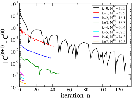
Figure 2: Absolute difference between neighbouring iterations of the Euler constant for the R14i60$\Uparrow$ initial data set. $k$ labels AMR adjustment iterations, and $n$ the inner iterative loop at fixed grid-resolution.

We begin by looking at the convergence of the Euler constant, $C$. In figure 2 we plot the absolute difference in $C$ between neighbouring iterations for the eight different resolutions used in the initial data solve. In the figure we see that at a given resolution these differences decrease exponentially with iteration as expected for the relaxation scheme employed (cf. Eq. 54). Meanwhile the differences also decrease with increasing resolution. We find similar results for all the other initial data sets we consider.

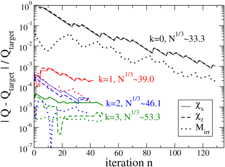
Figure 3: Fractional difference from desired values of black hole spin and mass. Shown is the solution of R14i60$\Uparrow$ initial data set as a function of iteration count. The four colours represent the four different resolutions $k=0,\ldots,3$ at which the black hole spin is measured.

Next, we will look at the properties of the black hole to verify that they converge as expected in the presence of a spinning neutron star, using again R14i60$\Uparrow$ as our example. We focus on the black hole spin $\vec{\chi}_{\rm BH}$ which is controlled by the parameter $\Omega_{j}^{\rm BH}$ in Eq. 24, and the irreducible black hole mass, $M_{\rm irr}$ (cf. Eq. 46).

Figure 3 shows the fractional difference for these quantities to their desired target value. The difference is plotted as a funciton of iteration, for four different resolutions. Recall that the BH spin is only adjusted on iterations $k=0,1,2,3$, and not thereafter (cf. Step 5). In general we see a decrease in this difference with iteration, especially at the first resolution, therefore showing that the iterative solver is correctly driving the the black hole properties to the target values. Furthermore, that this difference decreases with resolution, and we are able to achieve an accuracy of about $10^{-5}$ in the BH spin and mass. Note that these differences continue to remain small for $k>3$.

Having established the convergence of the iterative procedure, we turn now to the global properties of the solution, continuing to focus on the R14i60$\Uparrow$ ID set. We first consider the Hamiltonian and momentum constraints, computed as

$$H =||\frac{R_{\Psi}}{8\Psi^{5}}||,$$ (59)

$$M =||\frac{R_{\beta}}{2\alpha\Psi^{4}}||,$$ (60)

where $R_{\Psi}$ and $R_{\beta}$ are the residuals of Eqs. 15 and 16, respectively, and $||.||$ represents the $L2$ norm over all collocation points of the computational domain. The constraints for this ID set are shown in figure 4. We find exponential convergence in the constraints, as expected for spectral methods. The increase at the second iteration ($k=1$) arises because the neutron star spin is only activated in the second iteration (cf. step 2).

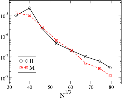
Figure 4: The Hamiltonian and momentum constraints for the R14i60$\Uparrow$ initial data set as a function of resolution. We find exponential convergence in both.

Finally, we look at the properties of the neutron star. As noted in Eq. 55, the neutron star surface is expressed as a sum of spherical harmonics. To evaluate the convergence of the surface location, we define the quantity

$$\Delta c^{(k)}=\sqrt{\sum_{l,m}\left(c_{lm}^{(k)}-c^{(k_{\rm max})}_{lm}\right)^{2}},$$ (61)

where $k$ represents the current resolution, and $k_{\rm max}$ represents the highest resolution. This quantity is plotted in figure 5. Similar to the black hole surface, the neutron star surface is only computed for the first four resolutions, and so we have three data points shown. We find exponential convergence in this quantity. We also look at the convergence of the neutron star spin $\chi_{\rm NS}$ measured at each resolution. In figure 5, we plot the fractional difference in $\chi_{\rm NS}$ between neighbouring resolutions. That is, we plot

$$\delta\chi^{(k)}_{\rm NS}=\frac{\big{|}\chi^{(k+1)}_{\rm NS}-\chi^{(k)}_{\rm NS}\big{|}}{\chi^{(k)}_{\rm NS}}.$$ (62)

Figure 5 exhibits exponential convergence, although there are two disinctly different slopes in the data, once we cease to update the NS surface for $k\geq 4$. Nevertheless, we are able to measure the spin to an accuracy of about $10^{-6}$. We have omitted the first data point of $\delta\chi^{(k)}_{\rm NS}$, because the NS spin is not activated for $k=0$ (cf. Step.  2).

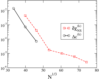
Figure 5: Accuracy of neutron star properties for the solution of R14i60$\Uparrow$. Plotted are the accuracy of the NS surface, $\Delta c^{(k)}$, as defined in Eq. 61 and the fractional accuracy of the NS spin (equation 62).

The above data all show that we have established the convergence of our initial data solver, by showing exponential convergence of the iterative solver, the black hole properties, neutron star properties, and the constraints.

4.3 Broader exploration of parameter space

All initial-data sets constructed so far share the same black hole mass and black hole spin-magnitude, $M_{\rm BH}=9.8_{\odot}$ and $\chi_{\rm BH}=0.9$. In this section, we relax these restrictions, and also explore the range of possible neutron star spins our code is capable to construct. In total, we consider three additional sequences of initial-data sets:

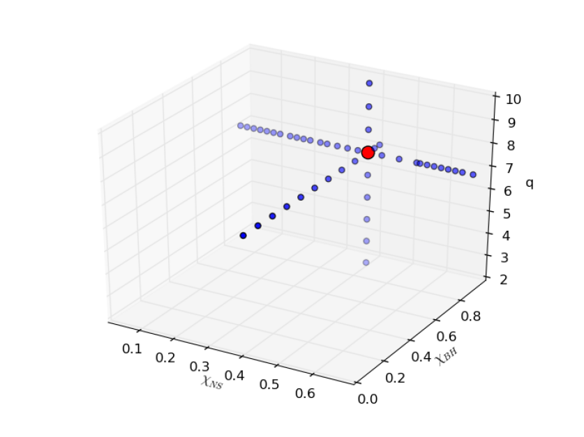
Figure 6: Parameter space exploration. Starting from R14i0$\Uparrow$(large red circle) we vary (i) the BH spin $\chi_{\rm BH}$, (ii) the NS spin $\chi_{\rm NS}$ and (iii) the black hole mass $M_{\rm BH}$, indicated by the mass-ratio $q$.

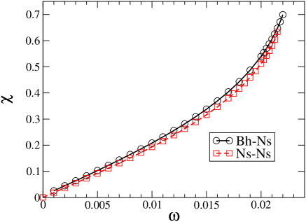
Figure 7: Neutron star spin $\chi$ as a function of neutron star spin parameter $\omega$ for a sequence of initial data sets. The black hole spin is constant at $\chi=0.9$ and the mass ratio is $q=7$. The dashed red curve is from NS-NS binaries, with somewhat different neutron star parameters.

First, we consider a sequence that varies the neutron star spin from $\chi_{\rm NS}=0$ to $\chi_{\rm NS}\sim 0.7$, keeping it aligned with the orbital angular momentum. In these initial data sets, the other binary parameters are the same as in the R14i0 runs. Namely, the neutron star mass, equation of state, black hole mass, black hole spin, initial separation and orbital angular frequency. Second, we consider a sequence of runs where we vary the black hole spin from $\chi_{\rm BH}=0$ to $\chi_{\rm BH}=0.99$, while keeping the other binary parameters as in the R14i0$\Uparrow$ run. Finally, we consider a sequence of runs where we vary the mass ratio from $q=2$ to $q=10$. Figure 6 summarizes all the initial data sets along the axes of $\chi_{\rm NS}$, $\chi_{\rm BH}$ and $q$.

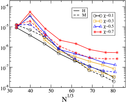
Figure 8: Hamiltonian (solid curves) and momentum (dotted curves) constraints for four different neutron star spins.

We begin by varying the neutron star rotation parameter $\omega$. The parameters in this sequence are otherwise the same as in the R14i0 data sets, and the neutron star spin is kept aligned with the orbital angular momentum. In Fig. 7 we plot the measured neutron star spin $\chi_{\rm NS}$ as a function of the code parameter $\omega$ for the full sequence. As expected, we find a linear relationship at low $\omega$, but the relationship becomes non-linear at higher $\omega$, as the neutron star’s size, and thus moment of inertia, becomes an appreciable function of spin. We find that the solver breaks down around $\chi_{\rm NS}\sim 0.7$, which is the maximum spin parameter for neutron stars found in [72]. Figure 7 also shows the corresponding $\chi_{\rm NS}$ vs. $\omega$ curve for a binary neutron star of mass-ratio $q=1$ with both stars carrying the same aligned spin magnitude as presented in [53]. The NS-NS data use different NS parameters, with mass $M_{\rm ADM}=1.64M_{\odot}$ and equation of state parameter $\kappa=123.6$. Nevertheless, the curves remain very close to each other in shape, indicating that the method to impart NS rotation [45] performs similarly for mixed BH-NS binaries and for NS-NS binaries [53].

To investigate numerical convergence of the initial-data sets presented in figure 7, we plot in figure 8 the Hamiltonian and momentum constraints for a subset of the generated initial data sets, with $\chi\sim{0.1,0.3,0.5,0.7}$. In general we find the expected exponential convergence, but there are a few features worth discussing in the data. The increase in the constraints between the lowest and second-lowest resolution ($k=0$ vs. $k=1$) arises because the spin is only activated at the second-lowest resolution, cf. step 2. This jump in constraints monotonically increases with the spin-parameter $\omega$, as we might expect, because the solver has a more difficult task in adjusting to the abrupt activation of a larger spin. We also note that at high resolution, in the $\chi\sim 0.7$ curve, we lose exponential convergence and the curves flatten out around $10^{-6}$. This is likely a sign that the accuracy of the solver is becoming limited, likely by approximations that go into the solver. $\chi\sim 0.7$ is around the maximum theoretical neutron star spin, so such difficulties are expected.

Continuing the exploration of parameter space, we next vary the black hole spin $\chi_{\rm BH}$. In partiuclar, we vary the black hole spin from $\chi_{\rm BH}=0$ to $\chi_{\rm BH}=0.99$, keeping it aligned with the orbital angular momentum. The other binary parameters are kept the same as in the ${\tt R14i0\Uparrow}$ initial data set, specifically $\vec{\omega}_{\rm NS}=0.017\hat{z}$ and $q=7$. In Figs. 9 we plot the Hamiltonian and momentum constraints, respectively, for this sequence. We find exponential convergence in all cases. It is interesting to note that the constraints seem to be lowest at the highest black hole spins, $\chi_{\rm BH}=0.95$ and $\chi_{\rm BH}=0.99$, while one might expect these to be the most challenging cases.

            

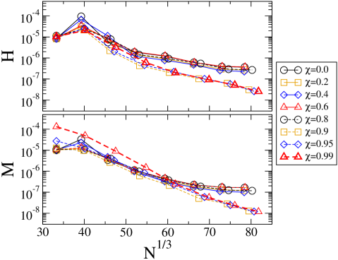
Figure 9: Hamiltonian constraint (top panel) and momentum constraint (bottom panel) versus resolution for our sequence of binaries where the black-hole spin is varied from $\chi_{\rm BH}=0$ to $\chi_{\rm BH}=0.99$. The NS spin parameter is kept constant at $\vec{\omega}_{\rm NS}=0.017\hat{z}$ and the mass ratio is $q=7$.

Since this work focuses on neutron star spin, it is interesting to consider how the measured neutron star spin, $\chi_{\rm NS}$ couples to other binary parameters. To lowest order, it should depend only on $\omega_{\rm NS}$, but in practice it may also depend on the parameters of the black hole or of the orbit. For the sequence of initial data sets of varying $\chi_{\rm BH}$, figure 10 presents the neutron star spin $\chi_{\rm NS}$ as a function of $\chi_{\rm BH}$. $\chi_{\rm NS}$ is nearly constant, dropping by less than 1% between $\chi_{\rm BH}=0$ and $\chi_{\rm BH}=0.99$, confirming that the spin specification for the neutron star almost completely decouples from the BH spin.

Figure 10: Neutron star spin $\chi_{\rm NS}$ as a function of black hole spin $\chi_{\rm BH}$ for this sequence. We notice a small downward linear trend.

Finally, we consider a sequence of initial-data sets that varies the mass ratio from $q=2$ to $q=10$. In this sequence we keep the other binary parameters the same as in the ${\tt R14i0\Uparrow}$ initial data set and we keep the orbital parameters $M\Omega$ and $D/M$ constant.

As the mass-ratio changes, we expect that the orbital frequency needed to achieve low eccentricity will also somewhat change. We do not model this effect, but rather keep all other binary parameters are the same as in the R14i0$\Uparrow$ run. In particular, the orbital parameters $M\Omega$ and $D/M$ are constant. While not the most accurate way of choosing these parameters, as it is only correct to Newtonian order, it suffices for the present purpose of testing robustness of the initial-data solver.

To estimate the impact on the eccentricity of the constructed initial-data sets, we use the post-Newtonian expansion of the orbital frequency of a BBH in a circular orbit (Eq. 228 of [73]):

$$\Omega^{2}=\frac{GM}{r^{3}}\left(1+(-3+\nu)\gamma+\left(6+\frac{41}{4}\nu+\nu^{2}\right)\gamma^{2}+...\right).$$ (63)

Here $\nu=m_{1}m_{2}/(m_{1}+m_{2}^{2})=q/(1+q)^{2}$ is the symmetric mass ratio, and $\gamma=GM/Dc^{2}$. Keeping $D$ and $M$ constant, the quantity $M\Omega$ varies by approximately 3% in the mass ratio range we consider. Therefore, we expect that the eccentricity of our initial-data sets varies by only a few percent between $q=2$ and $q=10$.

             

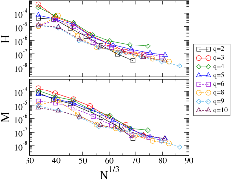
Figure 11: Hamiltonian constraint (top panel) and momentum constraint (bottom panel) versus resolution for our sequence of binaries where the mass ratio is varied from $q=2$ up to $q=10$. The NS spin parameter is kept constant at $\vec{\omega}_{\rm NS}=0.017\hat{z}$ and the black hole spin is $\chi_{\rm BH}=0.9$.

To assess convergence, we plot the Hamiltonian and momentum constraints for this sequence in Fig. 11. We find exponential convergence in all cases. Interestingly, no clear pattern in $q$-space emerges.

Figure 12 plots the neutron star spin as a function of mass-ratio. Having kept $\vec{\omega}_{\rm NS}$ constant across this sequence, we indeed find that the physical NS spin is approximately constant, too, varying less than $2$ percent. Although there is not a great amount of variation, apart from $q=2$, there is a clear trend of $\chi_{\rm NS}$ decreasing with $q$. Again, however, the effect is quite small and we do not seek to explain it.

Figure 12: Neutron star spin $\chi_{\rm NS}$ as a function of mass ratio $q$ for this sequence. We notice a small downward trend for $q\geq 3$.

5 Conclusion

In compact object binaries containing neutron stars, the spin of the neutron star(s) forms part of the parameter space of such binaries. In order to constrain neutron star spin directly from gravitational wave observations, one must know the impact of the neutron star spin on the evolution of the compact object binary, i.e. on the emitted waveforms and on the electro-magnetic signature.

This paper lays foundations for such studies by constructing initial-data sets of BH-NS binaries with arbitrary neutron star spins. To our knowledge, this is the first time initial data has been created for BH-NS binaries with spinning neutron stars. To impart spin on the neutron star, we carry over the formalism developed by [45] and used in [48, 53, 51] to create initial data for NS-NS systems with arbitrary spins.

Two new numerical tricks were found to be necessary to get convergent initial data - setting a maximum radius out to which to apply $W^{i}=\epsilon^{ijk}\omega^{j}r^{k}$, and only activating the neutron star spin after the first AMR-iteration of the initial data solver has completed. We create initial data sets across a large portion of the BH-NS binary parameter space.

First, we present a comprehensive study of initial-data sets with various NS spins, restricting to $q=7$ and $\chi_{\rm BH}=0.9$. This first study spans three different equations of state (all $\Gamma=2$ polytropes), different neutron star spin magnitudes, different neutron star spin orientations, and four different black hole spin orientations. Subsequently, we construct initial data with spinning NS for mass-ratios from $q=2$ to $q=10$, and for black-hole spins $0\leq\chi_{\rm BH}\leq 0.99$, the latter well exceeding the standard Bowen-York limit on black hole spin [64, 74]. Finally, we explore the range of possible NS spin magnitudes, and find that the presented numerical techniques can successfully construct initial data with neutron star spins ranging from $\chi_{\rm NS}=0$ to $\chi_{\rm NS}\sim 0.7$ (near the maximum theoretical spin for neutron stars).

Future research will involve running evolutions of these, or similar, initial data sets. Some of the 36 initial data sets of our first study (Table 1) can be used to investigate how neutron star spin affects tidal disruption of the star by the black hole, and how it affects the disk that is formed. The orbital phase evolution can also be examined and compared to Post-Newtonian[75] or other analytic predictions such as Effective-One-Body (EOB) [76, 77, 78].

One can also explore the maximum mass of accretion disks and ejecta as a function of NS spin. Ref. [36] finds a very large disk with a black hole spin of $\chi=0.97$ and mass ratio $q=3$. Keeping these BH and NS parameters, but adding spin on the neutron star will cause the NS’ material to be less strongly bound and may increase the disk mass even further.

References

- [1] Abbott B P et al. (LIGO Scientific Collaboration, Virgo Collaboration) 2016 Phys. Rev. Lett. 116(6) 061102 (Preprint 1602.03837) URL http://link.aps.org/doi/10.1103/PhysRevLett.116.061102
- [2] Abbott B P et al. (Virgo, LIGO Scientific) 2016 Phys. Rev. Lett. 116 241103 (Preprint 1606.04855)
- [3] Hulse R A and Taylor J H 1975 Astrophys. J. 195 L51
- [4] Abadie J et al. (LIGO Scientific) 2010 Class. Quantum Grav. 27 173001 arXiv:1003.2480 (Preprint 1003.2480)
- [5] Li L X and Paczynski B 1998 Astrophys. J. 507 L59 (Preprint astro-ph/9807272)
- [6] Roberts L F, Kasen D, Lee W H and Ramirez-Ruiz E 2011 Astrophys. J. Lett. 736 L21 (Preprint 1104.5504)
- [7] Metzger B D and Berger E 2012 Astrophys. J. 746 48 (Preprint 1108.6056)
- [8] Piran T, Nakar E and Rosswog S 2013 Mon. Not. Roy. Astr. Soc. 430 2121–2136 (Preprint 1204.6242)
- [9] Rosswog S, Piran T and Nakar E 2013 Mon. Not. Roy. Astr. Soc. 430 2585–2604 (Preprint 1204.6240)
- [10] Tanaka M, Hotokezaka K, Kyutoku K, Wanajo S, Kiuchi K, Sekiguchi Y and Shibata M 2014 Astrophys. J 780 31 (Preprint %****␣paper.bbl␣Line␣50␣****1310.2774)
- [11] Baumgarte T W and Shapiro S L 2010 Numerical Relativity: Solving Einstein’s Equations on the Computer (New York: Cambridge University Press)
- [12] Lehner L and Pretorius F 2014 Ann. Rev. of Astron. & Astroph. 52 661–694 (Preprint 1405.4840)
- [13] Pfeiffer H P 2012 Class. Quantum Grav. 29 124004 (Preprint 1203.5166)
- [14] Shibata M and Uryu K 2007 Class. Quantum Grav. 24 S125–S138
- [15] Faber J A, Baumgarte T W, Shapiro S L, Taniguchi K and Rasio F A 2006 Phys. Rev. D73 024012
- [16] Foucart F, Deaton M B, Duez M D, O’Connor E, Ott C D, Haas R, Kidder L E, Pfeiffer H P, Scheel M A and Szilagyi B 2014 Phys. Rev. D 90 024026 (Preprint 1405.1121)
- [17] Foucart F, Buchman L, Duez M D, Grudich M, Kidder L E, MacDonald I, Mroue A, Pfeiffer H P, Scheel M A and Szilagyi B 2013 Phys. Rev. D 88 064017 (Preprint 1307.7685)
- [18] Foucart F, Duez M D, Kidder L E, Scheel M A, Szilágyi B and Teukolsky S A 2012 Phys. Rev. D 85 044015 (Preprint 1111.1677)
- [19] East W E, Pretorius F and Stephens B C 2012 Phys. Rev. D 85 124009 (Preprint 1111.3055)
- [20] Shibata M and Uryu K 2006 Phys. Rev. D74 121503
- [21] Foucart F, Deaton M B, Duez M D, Kidder L E, MacDonald I, Ott C D, Pfeiffer H P, Scheel M A, Szilagyi B and Teukolsky S A 2013 Phys. Rev. D 87 084006 (Preprint 1212.4810)
- [22] Foucart F, Duez M D, Kidder L E and Teukolsky S A 2011 Phys. Rev. D 83 024005 (Preprint arXiv:1007.4203[astro-ph.HE])
- [23] Kawaguchi K, Kyutoku K, Nakano H, Okawa H, Shibata M and Taniguchi K 2015 Phys. Rev. D 92 024014 (Preprint 1506.05473)
- [24] Etienne Z B, Liu Y T, Shapiro S L and Baumgarte T W 2009 Phys. Rev. D79 044024
- [25] East W E, Paschalidis V and Pretorius F 2015 (Preprint 1503.07171)
- [26] East W E, Pretorius F and Stephens B C 2012 Phys. Rev. D 85 124009
- [27] Stephens B C, East W E and Pretorius F 2011 Astrophys.J. 737 L5 (Preprint 1105.3175)
- [28] Duez M D, Foucart F, Kidder L E, Ott C D and Teukolsky S A 2010 Class. Quantum Grav. 27 114106 (Preprint 0912.3528)
- [29] Kyutoku K, Shibata M and Taniguchi K 2010 Phys. Rev. D 82 044049 (Preprint 1008.1460)
- [30] Chawla S, Anderson M, Besselman M, Lehner L, Liebling S L et al. 2010 Phys. Rev. Lett. 105 111101 (Preprint 1006.2839)
- [31] Paschalidis V, Ruiz M and Shapiro S L 2015 Astrophys. J. 806 L14 (Preprint 1410.7392)
- [32] Kiuchi K, Sekiguchi Y, Kyutoku K, Shibata M, Taniguchi K and Wada T 2015 Phys. Rev. D 92 064034 (Preprint 1506.06811)
- [33] Etienne Z B, Liu Y T, Paschalidis V and Shapiro S L 2012 Phys. Rev. D 85 064029 (Preprint 1112.0568)
- [34] Etienne Z B, Paschalidis V and Shapiro S L 2012 Phys. Rev. D 86 084026 (Preprint 1209.1632)
- [35] Foucart F, O’Connor E, Roberts L, Duez M D, Haas R, Kidder L E, Ott C D, Pfeiffer H P, Scheel M A and Szilagyi B 2015 Phys. Rev. D 91 124021 (Preprint 1502.04146)
- [36] Lovelace G, Duez M D, Foucart F, Kidder L E, Pfeiffer H P, Scheel M A and Szilágyi B 2013 Class. Quantum Grav. 30 135004 (Preprint 1302.6297)
- [37] Shibata M and Taniguchi K 2008 Phys. Rev. D77 084015 (Preprint 0711.1410)
- [38] Pannarale F, Berti E, Kyutoku K, Lackey B D and Shibata M 2015 (Preprint arXiv:1509.06209[gr-qc])
- [39] Deaton M B, Duez M D, Foucart F, O’Connor E, Ott C D, Kidder L E, Muhlberger C D, Scheel M A and Szilagyi B 2013 Astrophys. J. 776 47 (Preprint 1304.3384)
- [40] Kyutoku K, Ioka K and Shibata M 2013 arXiv:1305.6309 (Preprint 1305.6309)
- [41] Paschalidis V, Etienne Z B and Shapiro S L 2013 Phys. Rev. D 88 021504 (Preprint 1304.1805)
- [42] Kawaguchi K, Kyutoku K, Shibata M and Tanaka M 2016 Astrophys. J. 825 52 (Preprint 1601.07711)
- [43] Foucart F 2012 Phys. Rev. D 86 124007 (Preprint 1207.6304)
- [44] Baumgarte T W and Shapiro S L 2009 Phys. Rev. D 80 064009 (Preprint 0909.0952)
- [45] Tichy W 2011 Phys. Rev. D 84 024041 (Preprint 1107.1440)
- [46] East W E, Ramazanoglu F M and Pretorius F 2012 Phys. Rev. D 86 104053 (Preprint 1208.3473)
- [47] Tichy W 2012 Phys. Rev. D 86 064024 (Preprint 1209.5336)
- [48] Bernuzzi S, Dietrich T, Tichy W and Bruegmann B 2014 Phys. Rev. D 89 104021 (Preprint 1311.4443)
- [49] Kastaun W, Galeazzi F, Alic D, Rezzolla L and Font J A 2013 Phys. Rev. D 88 021501 (Preprint 1301.7348)
- [50] Tsatsin P and Marronetti P 2013 (Preprint 1303.6692)
- [51] Dietrich T, Moldenhauer N, Johnson-McDaniel N K, Bernuzzi S, Markakis C M, Bruegmann B and Tichy W 2015 Phys. Rev. D 92 124007 (Preprint arXiv:1507.07100[gr-qc])
- [52] Tsokaros A, Uryū K and Rezzolla L 2015 Phys. Rev. D 91 104030 (Preprint 1502.05674)
- [53] Tacik N, Foucart F, Pfeiffer H P, Haas R, Ossokine S, Kaplan J, Muhlberger C, Duez M D, Kidder L E, Scheel M A and Szilágyi B 2015 Phys. Rev. D 92 124012 (Preprint 1508.06986)
- [54] Ajith P 2011 Phys. Rev. D 84 084037 (Preprint 1107.1267)
- [55] Foucart F, Kidder L E, Pfeiffer H P and Teukolsky S A 2008 Phys. Rev. D 77 124051 (Preprint arXiv:0804.3787)
- [56] Henriksson K, Foucart F, Kidder L E and Teukolsky S A 2016 Class. Quant. Grav. 33 105009 (Preprint 1409.7159)
- [57] http://www.black-holes.org/SpEC.html
- [58] Pfeiffer H P and York J W 2003 Phys. Rev. D 67 044022
- [59] York J W 1999 Phys. Rev. Lett. 82 1350–1353
- [60] Cook G B and Pfeiffer H P 2004 Phys. Rev. D 70 104016
- [61] Buonanno A, Kidder L E, Mroué A H, Pfeiffer H P and Taracchini A 2011 Phys. Rev. D 83 104034 (Preprint 1012.1549)
- [62] Pfeiffer H P, Kidder L E, Scheel M A and Teukolsky S A 2003 Comput. Phys. Commun. 152 253–273 (Preprint gr-qc/0202096)
- [63] Haas R, Ott C D, Szilagyi B, Kaplan J D, Lippuner J, Scheel M A, Barkett K, Muhlberger C D, Dietrich T, Duez M D, Foucart F, Pfeiffer H P, Kidder L E and Teukolsky S A 2016 Phys. Rev. D93 124062 (Preprint 1604.00782)
- [64] Lovelace G, Owen R, Pfeiffer H P and Chu T 2008 Phys. Rev. D 78 084017
- [65] Cook G B and Whiting B F 2007 Phys. Rev. D 76 041501(R)
- [66] Cook G B, Shapiro S L and Teukolsky S A 1994 Astrophys. J. 422 227–242
- [67] Arnowitt R, Deser S and Misner C W 1962 The dynamics of general relativity Gravitation: An Introduction to Current Research ed Witten L (New York: Wiley) pp 227–265 (Preprint gr-qc/0405109)
- [68] York Jr J W 1979 Kinematics and dynamics of general relativity Sources of Gravitational Radiation ed Smarr L L pp 83–126
- [69] Ossokine S, Foucart F, Pfeiffer H P, Boyle M and Szilágyi B 2015 ArXiv:1506.01689 (Preprint 1506.01689)
- [70] Buchman L T, Pfeiffer H P, Scheel M A and Szilágyi B 2012 Phys. Rev. D 86 084033 (Preprint 1206.3015)
- [71] Szilágyi B 2014 Int. J. Mod. Phys. D 23 1430014 (Preprint 1405.3693)
- [72] Lo K W and Lin L M 2011 Astrophys.J. 728 12 (Preprint 1011.3563)
- [73] Blanchet L 2006 Living Rev. Rel. 9 4
- [74] Dain S, Lousto C O and Zlochower Y 2008 Phys. Rev. D 78 024039 (Preprint 0803.0351v2)
- [75] Blanchet L 2014 Living Rev. Rel. 17 2 URL http://www.livingreviews.org/lrr-2014-2
- [76] Buonanno A and Damour T 1999 Phys. Rev. D 59 084006 (Preprint gr-qc/9811091)
- [77] Taracchini A, Buonanno A, Pan Y, Hinderer T, Boyle M, Hemberger D A, Kidder L E, Lovelace G, Mroue A H, Pfeiffer H P, Scheel M A, Szilagyi B, Taylor N W and Zenginoglu A 2014 Phys. Rev. D 89 (R) 061502 (Preprint 1311.2544)
- [78] Pan Y, Buonanno A, Taracchini A, Kidder L E, Mroue A H et al. 2013 Phys. Rev. D 89 084006 (Preprint 1307.6232)
- [79] Loken C, Gruner D, Groer L, Peltier R, Bunn N, Craig M, Henriques T, Dempsey J, Yu C H, Chen J, Dursi L J, Chong J, Northrup S, Pinto J, Knecht N and Zon R V 2010 J. Phys.: Conf. Ser. 256 012026